The Role of Infrastructure in the Rural â€“ Urban Digital Divide

The Role of Infrastructure in the Rural – Urban Digital Divide

Brian E. Whitacre Graduate Research Assistant

[email protected]

Bradford F. Mills Associate Professor

[email protected]

Department of Agricultural and Applied Economics Virginia Polytechnic Institute and State University

Selected Paper prepared for presentation at the American Agricultural Economics Association Annual Meeting, Providence, Rhode Island, July 24 – 27, 2005.

Copyright 2005 by Brian E. Whitacre and Bradford F. Mills. All rights reserved. Readers may make verbatim copies of this document for non-commercial purposes by any means, provided that this copyright notice appears on all such copies.

mailto:[email protected]

mailto:[email protected]

Introduction

Differences in residential Internet access rates (digital divides) have been well

documented for high and low education households (NTIA, 1999; 2000) and for high and

low income households (Pearce, 2001). Similarly, a divide between households in rural

and urban areas has been the focus of a number of studies (Malecki, 2003; Strover,

2001).1 Differences in rural and urban distributions of household characteristics have

been shown to explain a significant share of the rural – urban divide. Mills and Whitacre

(2003) find that differences in household characteristics, particularly lower income and

education levels in rural areas, account for approximately two-thirds of the rural – urban

gap in general residential Internet access in 2001. Less racial diversity, higher levels of

dual-headed households, older households heads, and lower rates of access from work in

rural areas relative to urban areas also contribute to the observed gap (McConnaughey

and Lader, 1998; NTIA, 2000; Rose 2003). Network externalities may also play a role.

Many Americans use the Internet to become more connected with their local community

(Horrigan, 2001). Hence, the value of the Internet to a household may increase with the

share of other households in the region that are connected.

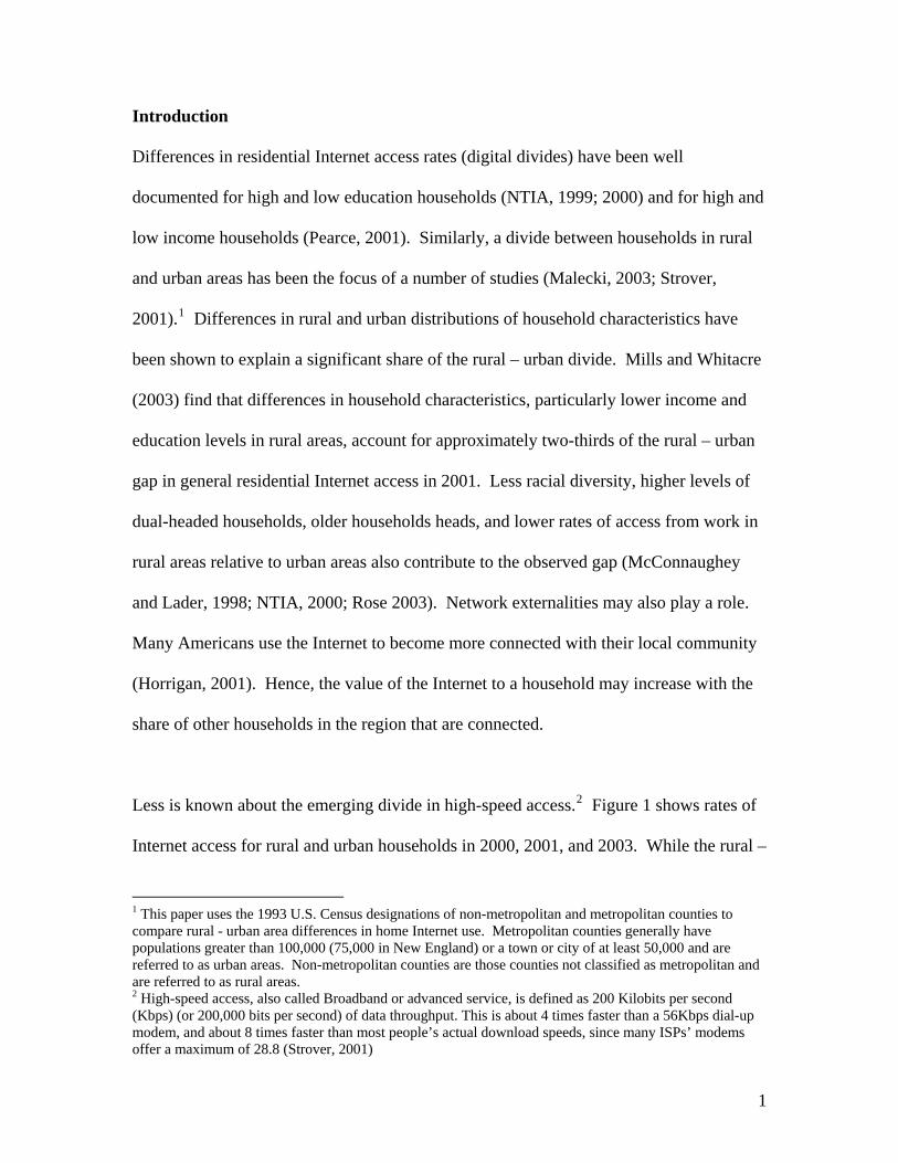
Less is known about the emerging divide in high-speed access.2 Figure 1 shows rates of

Internet access for rural and urban households in 2000, 2001, and 2003. While the rural –

1 This paper uses the 1993 U.S. Census designations of non-metropolitan and metropolitan counties to compare rural - urban area differences in home Internet use. Metropolitan counties generally have populations greater than 100,000 (75,000 in New England) or a town or city of at least 50,000 and are referred to as urban areas. Non-metropolitan counties are those counties not classified as metropolitan and are referred to as rural areas. 2 High-speed access, also called Broadband or advanced service, is defined as 200 Kilobits per second (Kbps) (or 200,000 bits per second) of data throughput. This is about 4 times faster than a 56Kbps dial-up modem, and about 8 times faster than most people’s actual download speeds, since many ISPs’ modems offer a maximum of 28.8 (Strover, 2001)

1

urban divide in general access has been relatively constant at around 13 percentage points

over this period, the divide in high-speed access has been increasing dramatically – from

3 percentage points in 2000 to 14 percentage points in 2003.3 There is reason to believe

that the factors underlying this emerging gap in high-speed access may be different from

those underlying the gap in general access. In particular, while basic dial-up service has

become nearly universally available, important differences in digital communications

technology (DCT) infrastructure exist in rural and urban areas that allows for high-speed

Internet access. Federal Communications Commission survey data in 2000 indicates that

while 70 percent of ZIP code areas in the U.S. have households that use high-speed

connections, these areas contain 95 percent of the population (Prieger, 2003). Hence, the

remaining 30 percent without any residential high-speed connections contain only 5

percent of the population, implying that, for the most part, those zip codes without high-

speed connections are low density regions and are rural in nature.

This paper focuses on the role of DCT infrastructure in the emerging divide in high-speed

residential Internet access. Three issues are explored in depth: (1) the recent diffusion of

DCT infrastructure in rural and urban areas of the U.S., (2) the contribution of DCT

infrastructure, as well as household characteristics and network externalities, to the

emerging divide in high-speed access, and (3) the potential role of DCT infrastructure in

closing the emerging divide in high-speed access.

3 All estimates, unless noted, are based on authors’ calculations using Current Population Survey Computer and Internet Use Supplements from 2000, 2001, and 2003.

2

Data and Descriptive Statistics

Several sources of empirical data are used in the paper. The household characteristics

and local rates of access (which serve as a proxy for network externalities) are obtained

from Current Population Survey Supplemental Questionnaires on Household Computer

and Internet Use. These nationally representative surveys of roughly 50,000 households

collect basic household member demographic and employment information on a monthly

basis, while the supplement focuses specifically on residential computer and Internet use

in 2000, 2001, and 2003. One drawback of this data is that the lowest level of geographic

information available on a household is rural or urban status within a state. Hence,

“local” rates of access cannot be calculated at the zip code or even county level. Rather,

they are average access rates for all rural (urban) households in the state.

Residential Internet access is defined by a positive response to the question, "Does

anyone in the household connect to the Internet from home?" Additionally, the survey

identifies whether the household connects via a dial-up modem or a higher-speed

connection.4 Table 1 provides information on the number of rural and urban households

in each year of the data, along with the number of households that had Internet and high-

speed access in those years. Although some households were omitted due to missing or

inconsistent data, there are still a large number of households in both the urban and rural

samples.

4 The 2000 CPS questionnaire only differentiates between dial-up and higher speed connections. The 2001 and 2003 questionnaires include categories for DSL, cable, satellite, and wireless (all of which are considered high-speed for the purposes of this paper).

3

Table 2 displays descriptive statistics for rural and urban area household characteristics

that previous research suggests might affect residential Internet access. Rural households

have, on average, lower education and income levels than their urban counterparts for all

years. Additionally, rural areas are less racially diverse, have older household heads, and

have a higher incidence of married couples than urban areas. Rural households are also

more likely to be headed by a male, have no children present, and have a retired

household head. It is also worth noting that rural households are much less likely to have

access at work (netatwork) when compared to their urban counterparts.

Network externalities (the value that a network member obtains increases as more

members enter the network) may play an important role in determining the magnitude of

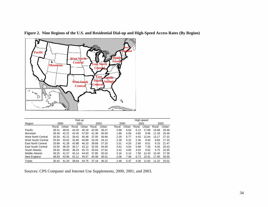
the benefits associated with residential Internet access. CPS data from 2000, 2001, and

2003 document substantial regional variation in Internet access that could give rise to

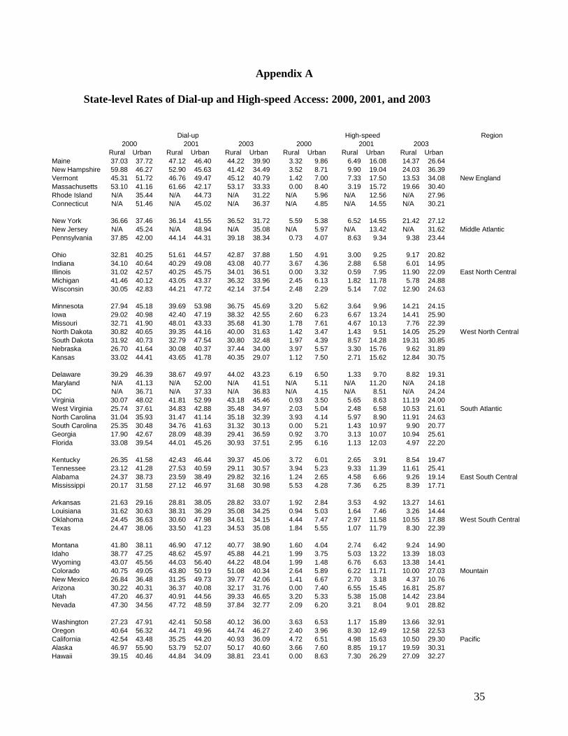
network externalities. Dial-up and high-speed access rates are given for nine regions of

the U.S. (Figure 2).5 For example, rural and urban households in the Pacific and New

England regions have higher rates of high-speed access than the national average.

Alternatively, the high-speed access rate in the West South Central region is well below

the national average. This variation potentially generates higher benefits from network

externalities in some regions than others. State-level residential rural and urban Internet

access rates are included in Appendix A, and are denoted “regdensity” in the analysis that

follows.

5 The nine regions are based on the breakout used in the Current Population Survey supplement. Analysis of states comprising each region indicates that rates of residential Internet access between states in a region are relatively similar (Appendix A).

4

An important contribution of the current paper is the construction of state level rural and

urban area measures of the availability of digital technology infrastructure. This measure

is constructed from two separate data sources on cable Internet and Digital Subscriber

Line (DSL) capacity.6 Information on county-level cable Internet capacity is

documented in the Television and Cable Factbooks for 2000, 2001, and 2003. Similarly,

the Tariff #4 dataset available from the National Exchange Carriers Association (NECA)

provides information on the DSL capability of every central office switch in the U.S

(approximately 38,000 in 2003), along with the city or town served by each central office

switch.7 The 2000, 2001, and 2003 versions of the dataset are used to estimate DSL

capacity in those years. A digital technology infrastructure index is then created for

every county (or city) by weighting the capability of various technologies in that county

(or city) by the population level.8 In order to mesh this index with household data from

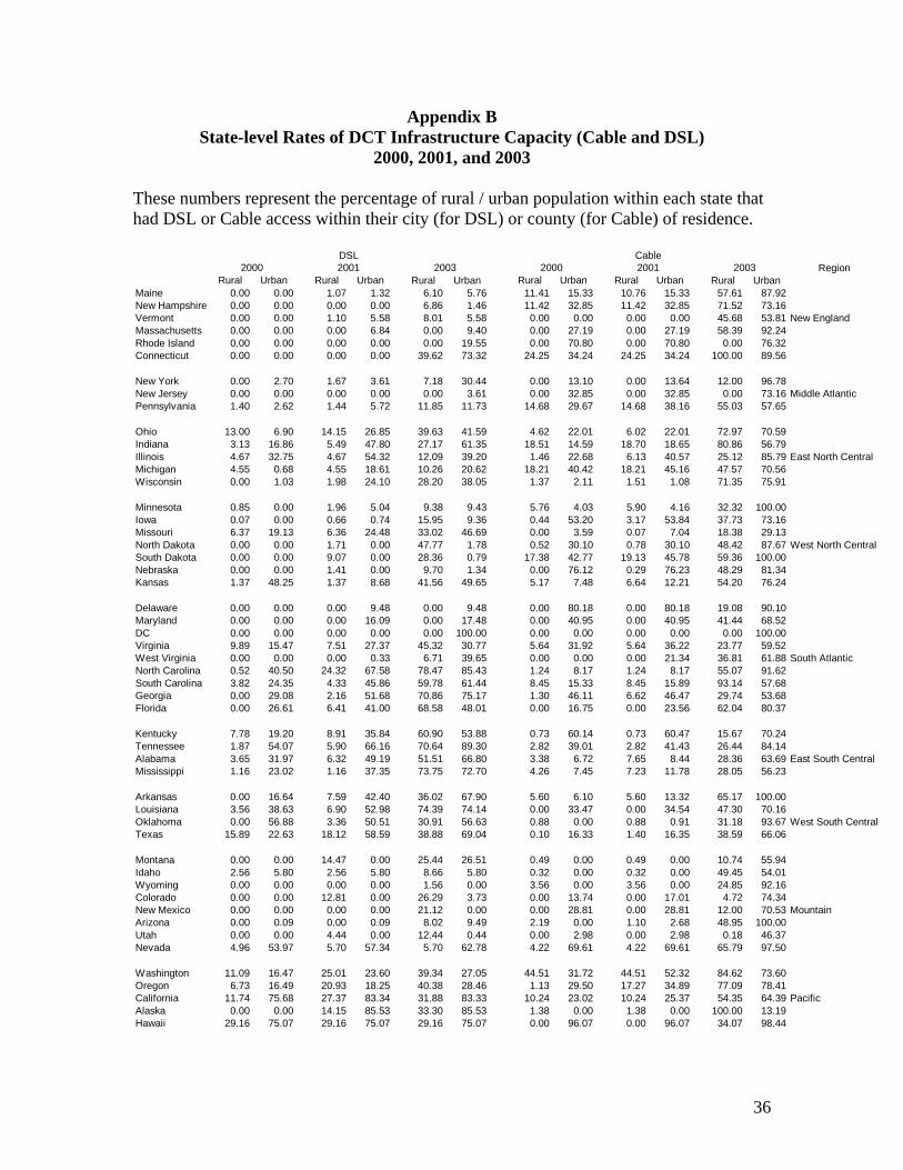
the CPS, it is further aggregated to rural / urban areas within a state. Hence, the ultimate

output from these data sources is the percentage of the population living in rural and

urban areas of each state that have DCT infrastructure (either DSL or cable) available to

them, or "DCT infrastructure capacity" (Appendix B).

6 Cable and DSL accounted for 99 percent of the high-speed market in 2003, with satellite and wireless connections accounting for the other 1 percent (FCC, 2003). 7 Tariff #4 data from 2003 indicates that most (59%) of these 38,000 central office switches are located by themselves, while the other 41% are co-located in “wire centers,” which house two or more switches. These switches may belong to many different telecommunications providers. 8 Data on city / county population levels is taken from the 2000 census, provided by the Bureau of Labor Statistics.

5

A country-level summary of the share of rural and urban population with DSL and cable

Internet capacity in their counties is presented in Table 3.9 While 2003 saw dramatic

increases in the percentage of both rural and urban populations with cable and DSL high-

speed infrastructure capacity, rural areas still lag behind urban areas. Further, the

percentage point gap is growing for cable Internet capacity. The diffusion of DCT

infrastructure has also been very different for various regions of the country. Information

on DCT infrastructure capacity in rural and urban areas of the nine regions of the U.S.

depicted in Figure 2 is provided in Table 4 for the years 2000, 2001, and 2003. Several

patterns are noticeable. Looking first at DSL, the capacity has increased remarkably in

the south - particularly in the rural areas. For all rural areas, DSL capacity increased

from 6.39 percent in 2001 to 29.55 percent in 2003 (an impressive 362 percent increase).

However, in the southern regions (South Atlantic, West South Central, and East South

Central), rural households saw increases of 401 percent, 637 percent, and 1,053 percent,

respectively. This increase is consistent with BellSouth’s aggressive deployment of DSL

starting in late 2001 (Pinkham Group, 2002). Other rural areas, such as those in the

Mountain, Middle Atlantic, and New England regions, continued to have relatively low

DSL capacity through 2003. Additionally, the diffusion of DSL capacity has slowed for

rural households in the Pacific and East North Central regions. While these regions had

relatively high capacity in 2000, their growth rates did not keep pace with those for rural

regions in the rest of the country. Finally, it is worth noting that the rural – urban

discrepancy in capacity has shown different trends in various regions of the country. For

instance, the Pacific region has consistently seen DSL capacity in rural areas lag behind

9 Infrastructure data on cable is available only at the county level, but DSL data is available at the city level, which allows for a lower level of detail on the percentage of the population with infrastructure capacity.

6

that in urban areas by approximately 25 percentage points from 2000 through 2003. On

the other hand, the rural population in the West North Central region has gone from

lagging their urban counterparts by 8 percentage points in 2000 to being 9 percentage

points higher in 2003! Alternatively, the gap has increased in the East North Central

region, going from 6 percentage points in 2000 to 17 percentage points in 2003.

Cable Internet diffusion has also shown different trends in various regions of the country.

Most of the diffusion occurred between 2001 and 2003, with capacity increasing by 39

percentage points in rural areas and 48 percentage points in urban areas. For all regions,

rural areas experienced increases in capacity during this period, but none quite as

dramatic as the West South Central region. Cable Internet capacity stood at less than 2

percentage points for the rural population in this region in 2001, and then skyrocketed to

46 percentage points in 2003 – a 2,213 percent increase! Similarly, in the Mountain

region cable Internet capacity increased from 15 percentage points to 74 percentage

points over this period. The diffusion was less striking in rural areas of the East South

Central region, with capacity increasing from 5 percentage points to 25 percentage points.

In general, the rural – urban gap in cable Internet capacity has increased between 2000

and 2003 (from 20 percentage points to 32 percentage points), but significant variance

exists within the country. The biggest change is in the Pacific region, where rural areas

actually have higher rates of cable Internet capacity in 2003 than urban areas (70

percentage points to 66 percentage points). This is drastically different from 2000, when

rural rates were 25 percentage points below urban rates. The East North Central region

has been relatively consistent over this period, with rural rates lagging urban rates by

7

approximately 12 percentage points each year. On the other hand, the diffusion of cable

Internet capacity in the Mountain region has occurred mainly in urban areas, as the urban

– rural discrepancy increased from 13 percentage points in 2000 to 47 percentage points

in 2003.

Thus, the exposure of the population to DCT infrastructure has varied not only across

rural and urban areas generally, but by region of the country. The role of this uneven

distribution of DCT infrastructure in the rural – urban digital divide is of yet

undetermined. Further, because the majority of both rural and urban households still

connect with dial-up access, the role of DCT infrastructure in the general digital divide

may be smaller than its role in the emerging high-speed digital divide. The next section

discusses the empirical model employed to understand the contribution of DCT

infrastructure and other factors to the rural – urban digital divide in general and high-

speed residential Internet access in particular.

Methodology

Basic Empirical Specification

The basic statistical model for capturing the influence of the factors discussed above

(household characteristics, network externalities, and DCT infrastructure) on Internet

adoption is specified as

iiiiiiii NDDHZXy επττγδβ ++++++= 21* 21 (1)

1=iy if 0 * ≥iy

0=iy if 0* <iy

8

where *iy is a latent measure of the benefits from residential Internet access relative to

the costs of household i, iy is the actual observation of household Internet access, iX is a

vector of household income levels, is a vector of household education levels, is a

vector of other household characteristics, and are the measures of DSL and cable

availability discussed in the previous section (dslaccess and cableaccess), is a

measure of the regional rate of Internet access (regdensity);

iZ iH

iD1 iD2

iN

πττγδβ ,,,,, 21 are the

respective associated parameter vectors, and iε is the statistical model’s error term. Due

to the discrete nature of the Internet adoption decision, a logit model is employed.10

Results

Parameter estimates for the household general access decision are presented in Table 5.

Parameter estimates for most of the independent variables have the expected signs for the

general access model. In particular, for all years, the parameter values for education are

positive, and increase as the level of education increases. This implies that, relative to a

household headed by an individual with no high school education, higher levels of

education increase the relative odds of a household having Internet access. Similarly, the

parameter values for income are significantly positive after income reaches $20,000

(faminc6). These parameters increase in value as the income level rises, meaning that the

propensity for Internet access increases with income. Additionally, for 2001 and 2003,

the presence of Internet access at work (netatwork), a married household head, and the

presence of one, two, or three children all positively impact the probability of Internet 10 Given this discrete nature, any binomial variable statistical model could have been chosen. However, the logit model had several benefits over its competitors – namely, that it restricts outcomes to the [0,1] interval (unlike the Linear Probability Model) and provides a closed form solution (unlike the probit model).

9

access. The significant positive coefficient on regdensity indicates that local connectivity

rates are important in the Internet access decision, with higher local rates resulting in

increased probability of access for a household. The age of the household head is also

positively related to access in all years; however, the negative coefficient on age2

indicates that the positive influence of age reaches a maximum and then starts to decline.

Households headed by Blacks and Hispanics are less likely to have Internet access for all

years, while households headed by other non-White racial groups are less likely to have

access in 2000 and 2003. Several variables are notably lacking significance. First, the

availability of cable (cableaccess) and DSL access (dslaccess) are not significant. Rural

status of the household (nm) is also insignificant in 2001 and 2003. This implies that,

after controlling for other variables such as education, income, and other household

characteristics, DCT infrastructure capacity and rural / urban status of the household do

not strongly influence the probability of general Internet access. The results also imply

that differences in education, income, and network externalities between rural and urban

households are likely more important in explaining the general access digital divide than

are differences in DCT infrastructure.

Model estimates with the same set of variables in the high-speed access decision yield

similar parameter estimates for many variables (Table 6). In particular, higher levels of

income and education increase the probability of high-speed access relative to households

headed by individuals with low-income (under $5,000 per year) and low education levels

(no high school diploma). However, only higher income levels (faminc10 - $40,000 or

higher) are significant in most of the regressions, and the parameter values jump

10

significantly for the highest level of income. Hence, having the highest level of income

(faminc13 - $75,000 or more) may be particularly important in determining high-speed

access. Internet access at work (netatwork) continues to be positively associated with

high-speed access, as does the proxy for network externalities (regdensity). Meanwhile,

households headed by Blacks and by Hispanics are still less likely to have high-speed

access than Whites and non-Hispanics, respectively.

The high-speed access model does exhibit a number of noteworthy differences from the

model for general access. First, rural status of the household has a significant and

negative effect on high-speed residential Internet access in the years 2001 and 2003. This

implies that even after controlling for differences in household characteristics (such as

education and income) between rural and urban households, location in a rural area

decreases the probability of high-speed access. Similarly, DSL capacity parameter

estimates are positive and significant in 2001 and 2003, meaning that higher DSL

infrastructure capacity was a significant factor for high-speed access. Interestingly, the

coefficient for cable access is negative in 2001, implying that higher availability of cable

Internet decreased the probability of high-speed access in this year, but was not

significant in 2000 and 2003. Another distinct difference between the high-speed and

general access model results is the lack of significance of chld1, chld2, or chld3

parameter estimates in any of the years. Apparently, the presence of children in the

household does not play a significant role in the high-speed adoption decision. This

result is somewhat surprising as large bandwidth is necessary for many common Internet

activities of children under the age of 18, such as music downloading and on-line gaming

11

(Horrigan, 2004). Another surprising result is the lack of significance of the age term

(peage) in 2000 and 2001, with only marginal significance in 2003. However, the

quadratic age term (age2) is negative and at least marginally significant in all years,

suggesting that the adoption propensity decreases rapidly with the age of the household

head. If young families are most likely to have high-speed access, this may in part

explain the lack of significance of children. Finally, households headed by a male are

more likely to have high-speed access in all years. This is in direct contrast to the model

for general access, where the sex of the household head was not significant in any year.

The result is, however, reminiscent of the early days of dial-up adoption when a

significant gender divide existed (Bimber, 2000).

Hence, significant differences do exist between the high-speed and general access logit

model results. This implies that the contribution of a group of characteristics to the rural

– urban digital divide could vary dramatically depending on the type of access in

question. The following section provides a more formal assessment of the importance of

individual factors to the rural – urban digital divide in general and high-speed access.

Decomposition of the Logit Model

A decomposition technique is employed to determine the contribution of each factor to

the rural – urban digital divide. The technique used is a non-linear version of the

Oaxaca-Blinder (Oaxaca, 1973; Blinder, 1973) decomposition, due to the non-linear

12

nature of the logit model.11 The standard (linear) Oaxaca-Blinder decomposition of the

general rural – urban digital divide in residential Internet access can be expressed as:

)ˆˆ(ˆ)( RURURURUXXXYY βββ −+−=− (2)

where G

Y is the average value of Internet access, G

X is a row vector for average values

of the independent variables, and is a vector of coefficient estimates for rural / urban

status G. Following Fairlie (2003), the decomposition for a non-linear equation, such as

, can be written as:

Gβ̂

)ˆ( βXFY =

⎥⎦

⎤⎢⎣

⎡−+⎥

⎦

⎤⎢⎣

⎡−=− ∑∑∑∑

====

RRRU N

iR

RRi

N

iR

URi

N

iR

URi

N

iU

UUiRU

NXF

NXF

NXF

NXFYY

1111

)ˆ()ˆ()ˆ()ˆ( ββββ (3)

where is the sample size for rural / urban status G. Equation (3) applies urban and

rural coefficient estimates to the two distinct groups of explanatory variables, and

. Equivalently, the decomposition can be written as:

GN

UiX

RiX

⎥⎥⎦

⎤

⎢⎢⎣

⎡−+

⎥⎥⎦

⎤

⎢⎢⎣

⎡−=− ∑∑∑∑

====

RRRU N

iU

RUi

N

iU

UUi

N

iR

RRi

N

iU

RUiRU

NXF

NXF

NXF

NXF

YY1111

)ˆ()ˆ()ˆ()ˆ( ββββ (4)

This first term on the right hand side of equations (3) and (4) represents the part of the

digital divide due to group differences in the distributions of the explanatory variables X.

The choice of which set of parameters to use (either in (3) or in (4)) is the

essence of the familiar "index problem" to the Oaxaca-Blinder decomposition, and can be

the source of significantly different results. Some studies suggest weighting the

parameters by using coefficient estimates from a pooled sample of the two groups

(Neumark, 1988; Oaxaca and Ransom, 1994). This approach results in the use of

Uβ̂ Rβ̂

11 This non-linear version of the Oaxaca-Blinder decomposition is similar to the procedure used in Mills and Whitacre (2003) and Fairlie (2003).

13

weighted average parameters ( instead of or ), and is valid when the "weighted

average" access rates are considered exemplary of the rates that would exist in the

absence of a digital divide (Oaxaca and Ransom, 1994).

β̂ Uβ̂ Rβ̂

In order to calculate the contributions from individual explanatory variables included in

the first term of (3) or (4), we must be able to “replace” a single rural characteristic (for

example, education level) with its urban counterpart. Hence, a one-to-one mapping of the

rural and urban samples is needed to establish an urban counterpart for each rural

observation. In order to create such a mapping, predicted probabilities of Internet access

are calculated for all observations (both rural and urban) using the specification in

equation (1). Since the sample size for urban households is larger than the sample size

for rural households, a sub-sample of urban households is randomly drawn equal in size

to the rural sample. This sampling procedure will clearly affect UY and , since both

are dependent on the households included in the sample. However, as discussed below,

results from the entire urban sample can be approximated by bootstrapping a large

number of urban samples and averaging the results of the decomposition.

UiX

The two individual samples (the full rural sample and random urban sub-sample) are then

ranked by predicted probability of Internet access. Hence, rural households that have

characteristics placing them high (low) in their distribution are matched with urban

households that have characteristics placing them high (low) in their distribution. To

accomplish the decomposition, let X1, X2, and X3 ∈ X be the three distinct sets of

independent variables discussed previously: X1 represents household characteristics, X2

14

represents network externalities, and X3 represents telecommunications infrastructure.

Using coefficient estimates from a logit regression of a pooled sample of both rural

and urban households, the independent contribution of X

β̂

1 to the digital divide can be

expressed as:12

).ˆˆˆˆ()ˆˆˆˆ(13322110332211

10 ββββββββ U

iUi

Ri

Ui

Ui

Ui

N

iR XXXFXXXF

N

R

+++−+++∑=

(5)

Similar expressions can be written for the contributions of X2 and X3. Hence, the

contribution of each group of variables to the gap equals the change in average predicted

probability from replacing the rural distribution with the urban distribution for that group

of variables while holding the distributions of the other groups constant.13 This

technique is particularly useful because the sum of the contributions from the individual

groups will be equal to the total contribution from all variables in the sample (Fairlie,

2003).

It is important to note that equation (5) deals only with the first term of the decomposition

shown in equations (3) and (4). The second term in equations (3) and (4) above

represents the portion of the gap due to rural - urban differences in underlying

parameters, and is not affected by differences in explanatory variables. The three

categories of independent variables discussed above, along with this residual portion,

make up the entire rural - urban digital divide in any given year. Thus, the framework

12 Note that since a pooled sample is used to obtain coefficient estimates, the decomposition uses weighted averages of the parameter estimates shown in equations (3) and (4). 13 Because of the non-linear form assumed by the use of the logit model, the contributions of X1, X2, and X3 depend on values of the other variables. Hence, the order of how the variables enter equations (3) and (4) may affect their individual contributions to the rural-urban digital divide. To account for this, the order in which variables enter the analysis will be varied, and the results will be compared.

15

will be useful in determining the roles played by the various categories for any given time

period.

General Access Decomposition Results

The results of the non-linear decomposition for general Internet access in 2000, 2001, and

2003 are presented in Table 7.14 The first two rows of Table 7 indicate the share of rural

and urban households with Internet access, and the third shows the resulting "digital

divide" for each of the three years of CPS data. The remainder of the table reports the

individual contributions from rural – urban differences in education, income, other

household characteristics, network externalities, and DCT infrastructure.

The difference between rural and urban general Internet access rates ranges from 12.8

percentage points in 2003 to 13.8 percentage points in 2000. As expected, differences in

education and income levels explain a large portion of this gap. Lower levels of

education in rural areas account for between 17 and 22 percent of the gap, while lower

levels of income account for between 34 and 36 percent of the gap. Differences in

network externalities also play an important role, as they make up between 29 and 40

percent of the gap in a given year. Other household characteristics do not have much

explanatory power, consistently making up less than 1 percent of the gap. However,

given the results of the general logit model (discussed in the previous section), the

minimal contribution of those factors grouped under “other household characteristics”

could mask significant offsetting effects, such as the positive impact of children in the

14 Unless noted otherwise, all decompositions use 1,000 random samples of urban households. The results remain essentially unchanged when either 100 or 10,000 random samples were used.

16

household or the negative impact of a Black or Hispanic household head. Rural – urban

differences in DCT infrastructure explain very little, comprising only between –0.1 to 4

percent of the gap. The decompositions indicate that group differences in all of the

included variables explain between 87 and 97 percent of the gap in general access. These

high shares of the gap explained by characteristic differences suggest that only a

relatively small portion of the gap (between 3 and 13 percent) is left unexplained by the

included variables and is attributable to parameter differences in rural and urban areas.

The non-linearity of the logit model implies that the results may be sensitive to the order

in which the variables are included. To explore this possibility, Table 8 reverses the

order of the explanatory variables. Most of the estimates are very similar to those

obtained with the original ordering; however two significant shifts occurred in the 2000

estimate. The role played by education jumps from 19 percent under the initial orderings

to 26 percent when the orderings are reversed, and other household characteristics shift

from explaining –2 percent of the divide to explaining –9 percent. The total contribution

remains the same in both cases because the sum of the individual contributions

necessarily equals the first term on the right-hand side of equations (3) and (4). As

Fairlie (2003) notes, the sensitivity of the order in which the variables are introduced is

dependent on the initial location in the logistic distribution and the movement inflicted on

this distribution by switching characteristics of rural and urban households. Fairlie

suggests experimenting with the ordering in order to verify the robustness of the results.

While there are 5! = 120 different orderings for 2000, 2001, and 2003, approximately 10

different orderings were attempted for each year, with all estimates lying in the intervals

17

created by the results in Tables 7 and 8. Thus, while some differences exist when the

ordering is varied, the dominant factors remain the same in all years.

High-speed Access Decomposition Results

Comparable results are obtained when a similar decomposition is performed for high-

speed access. High-speed access rates for rural and urban areas over the period 2000 –

2003 are shown in the first two rows of Table 9. As the third row of the table indicates,

the high-speed divide has increased from 3 percentage points in 2000 to 14 percentage

points in 2003. Turning to the contributions of various factors, education differences

make up between 5 and 9 percent of the divide over these years, while income levels

make up between 21 and 27 percent. It is interesting to note that the contribution of both

of these factors is below their contributions to the general divide. Differences in other

household characteristics consistently account for approximately 7 percent of the high-

speed divide, which is far above their aggregate contribution to the general divide.

Network externalities play the largest role in the high-speed divide, making up between

23 to 40 percent. This percentage is similar to the results for general access. DCT

infrastructure differences make up approximately 6 percent of the divide in 2003, but

actually increase the divide in 2000 and 2001. Reversing the order in which the variables

were introduced produces the results shown in Table 10. Again, the results are similar

under this re-ordering, with one exception being the impact of other household

characteristics – switching from explaining around 7 percent in all years under the initial

ordering to explaining –2 percent under the re-ordering. Additionally, the impact of

education increases from between 5 – 9 percent to between 9 – 13 percent of the total

18

gap. However, the dominant factors (income levels and network externalities) remain the

same under this re-ordering. Including all of the variables explained between 55 and 83

percent of the high-speed access digital divide.

Discussion and Policy Implications

Historically, the primary course of action of the federal, state, and local governments to

address the rural – urban digital divide has been to provide subsidies for DCT

infrastructure in low-density regions (Leighton, 2001). However, the results of the

decompositions indicate that the presence of DCT infrastructure is not a major factor in

either the general or high-speed divide between rural and urban areas. Rather,

differences in education and income, along with network externalities, are the most

important factors for both the divide in general Internet access and the emerging divide in

high-speed access.

Since DCT infrastructure is essentially a necessary condition for residential high-speed

access, its lack of significance remains somewhat puzzling. One concern is whether the

results change dramatically if network externalities are excluded from the model. Given

that local rates of high-speed access may indicate some measure of DCT infrastructure

capacity, the proxy for network externalities may be capturing some of the effects of such

capacity. When the high-speed access decomposition is performed for this alternative

specification, the impact of DCT infrastructure does increase, but not dramatically. For

all years, differences in DCT infrastructure capacity make up between 1 and 8 percent of

the high-speed divide. Meanwhile, income differences continue to account for over 22

19

percent of the divide. A second concern is that the aggregate nature of the DCT

infrastructure measures may be masking underlying local relationships between

infrastructure and high-speed access. Data constraints do not allow us to fully address

this concern, and further research is needed on this issue.

Looking at the high-speed divide from a policy standpoint, the results indicate that efforts

to close the emerging high-speed divide should focus on the underlying education and

income gap between rural and urban areas. The importance of network externalities is

also evident, but does this justify the presence of initial subsidies for high-speed access in

areas with low adoption rates? The continued contribution of externalities for both dial-

up and high-speed access lends support for such subsidies, and further research may need

to identify the "tipping point" where the impact of subsidies is largest. The question of

whether public policies should address DCT infrastructure also arises. While the analysis

demonstrates that differences in DCT infrastructure capacity are not a driving force

behind the divide, significant differences in capacity still exist between rural and urban

areas. Initial evidence on diffusion is mixed, with the rural – urban gap in DSL capacity

shrinking while the gap in cable Internet capacity is growing. Given the short time frame

that these technologies have been available, market mechanisms may need additional

time to diffuse capacity to more remote areas. The current analysis does not lend support

for policies that promote infrastructure capacity in rural areas as the sole intervention to

bridge the emerging gap in high-speed access.

20

References

Bimber, B. 2000. “Measuring the Gender Gap on the Internet.” Social Science Quarterly. 81: 868-876.

Blinder, A. 1973. "Wage Discrimination: Reduced Form and Structural Variables."

Journal of Human Resources. 8: 436-455. Drabenstott, M. 2001. “New Policies for a New Rural America.” InternationalRegional

ScienceReview. 24, 1:3-15. Fairlie, R. 2003. "An Extension of the Blinder-Oaxaca Decomposition Technique to

Logit and Probit Models." Economic Growth Center: Yale University. Paper Number 873.

Federal Communications Commission – Industry Analysis and Technology Division.

2003. High Speed Services for Internet Access: Status as of June 30, 2003. Available at http://www.fcc.gov/wcb/iatd/comp.html

Horrigan, J.B. 2001. Online Communities: Networks that Nurture Long-Distance

Relationships and Local Ties. Pew Internet & American Life Project. http://pewinternet.org/

Horrigan, J.B. 2004. PEW Internet Data Project Memo: Home Broadband Adoption has

Increased 60% in the past year and use of DSL Lines is Surging. Pew Internet a& American Life Project. http://pewinternet.org/

Leighton, W.A. 2001. “Broadband Deployment and the Digital Divide.” Cato Policy

Analysis No. 410. August 7. Malecki, E.J. 2003. "Digital Development in rural areas: potentials and pitfalls."

Journal of Rural Studies 19: 201-214. McConnaughey, J., and W. Lader. 1998. Falling Through the Net II: New Data on the

Digital Divide. National Telecommunications and Information Administration, http://www.ntia.doc.gov/ntiahome/net2/falling.html

Mills, B.F. and B. Whitacre. 2003. "Understanding the Non-Metropolitan –

Metropolitan Digital Divide." Growth and Change. 34,2: 219-243. National Telecommunications and Information Administration and Economics Statistics

Administration. 2000. Falling Through the Net: Towards Digital Inclusion. U.S. Department of Commerce: Washington, D.C.

Neumark, D. 1988. "Employers Discriminatory Behavior and the Estimation of Wage

Discrimination." Journal of Human Resources. 23: 279-295.

21

http://www.fcc.gov/wcb/iatd/comp.html

http://pewinternet.org/

http://pewinternet.org/

http://www.ntia.doc.gov/ntiahome/net2/falling.html

Oaxaca, R. 1973. “Male-Female Differentials in Urban Labor Markets.” International

Economic Review. 14: 693-709. Oaxaca, R and M. Ransom. 1994. "On Discrimination and Decomposition of Wage

Differentials." Journal of Econometrics. 61: 5-21. Pearce, A. 2001. "Closing the Gap." America's Network. Sep. 1. Available at

http://www.americasnetwork.com/americasnetwork/article/articleDetail.jsp?id=12 Pinkham Group. 2002. “DSL Deployment Analysis of RBOCs and Independent LECs

in Metropolitan and Rural Areas – Q4 2001.” Available at http://www.dslprime.com/a/pinkham_deployment.htm

Prieger, J. 2003. “The supply side of the digital divide: Is there equal availability in the

broadband Internet access market?” Economic Inquiry. 41,2: 346 - 363. Rose, R. 2003. Oxford Internet Survey Results. The Oxford Internet Institute: The

University of Oxford, UK. Strover, S. 2001. "Rural Internet Connectivity." Telecommunications Policy 25: 331-

347. Warren Publishing Inc. 2000. Television and Cable Factbook, Cable and Services.

Number 68: Cable Volumes 1-2. Washington, D.C. Warren Publishing Inc. 2001. Television and Cable Factbook, Cable and Services.

Number 69: Cable Volumes 1-2. Washington, D.C. Warren Publishing Inc. 2003. Television and Cable Factbook, Cable and Services.

Number 71: Cable Volumes 1-2. Washington, D.C.

22

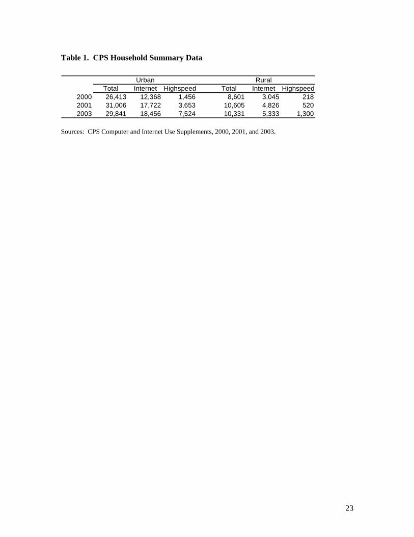
http://www.americasnetwork.com/americasnetwork/article/articleDetail.jsp?id=12

http://www.dslprime.com/a/pinkham_deployment.htm

Table 1. CPS Household Summary Data

Urban RuralTotal Internet Highspeed Total Internet Highspeed

2000 26,413 12,368 1,456 8,601 3,045 2182001 31,006 17,722 3,653 10,605 4,826 5202003 29,841 18,456 7,524 10,331 5,333 1,300

Sources: CPS Computer and Internet Use Supplements, 2000, 2001, and 2003.

23

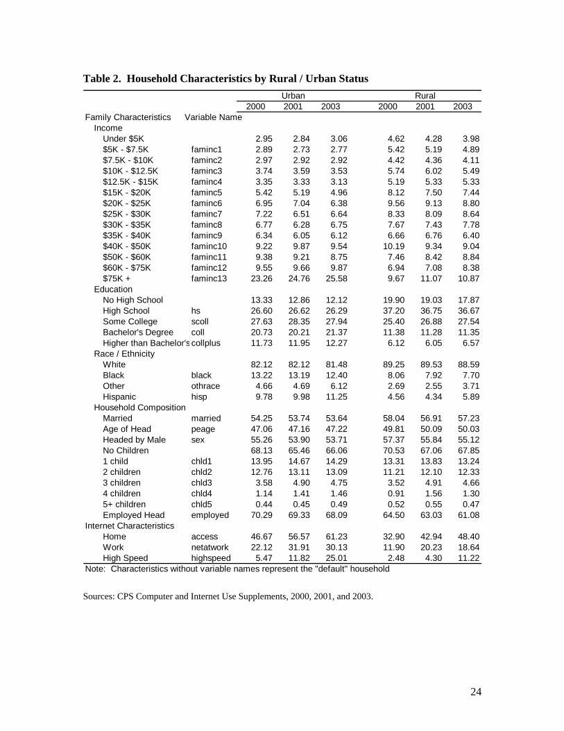
Table 2. Household Characteristics by Rural / Urban Status Urban Rural

2000 2001 2003 2000 2001 2003Family Characteristics Variable Name

IncomeUnder $5K 2.95 2.84 3.06 4.62 4.28 3.98$5K - $7.5K faminc1 2.89 2.73 2.77 5.42 5.19 4.89$7.5K - $10K faminc2 2.97 2.92 2.92 4.42 4.36 4.11$10K - $12.5K faminc3 3.74 3.59 3.53 5.74 6.02 5.49$12.5K - $15K faminc4 3.35 3.33 3.13 5.19 5.33 5.33$15K - $20K faminc5 5.42 5.19 4.96 8.12 7.50 7.44$20K - $25K faminc6 6.95 7.04 6.38 9.56 9.13 8.80$25K - $30K faminc7 7.22 6.51 6.64 8.33 8.09 8.64$30K - $35K faminc8 6.77 6.28 6.75 7.67 7.43 7.78$35K - $40K faminc9 6.34 6.05 6.12 6.66 6.76 6.40$40K - $50K faminc10 9.22 9.87 9.54 10.19 9.34 9.04$50K - $60K faminc11 9.38 9.21 8.75 7.46 8.42 8.84$60K - $75K faminc12 9.55 9.66 9.87 6.94 7.08 8.38$75K + faminc13 23.26 24.76 25.58 9.67 11.07 10.87

EducationNo High School 13.33 12.86 12.12 19.90 19.03 17.87High School hs 26.60 26.62 26.29 37.20 36.75 36.67Some College scoll 27.63 28.35 27.94 25.40 26.88 27.54Bachelor's Degree coll 20.73 20.21 21.37 11.38 11.28 11.35Higher than Bachelor'scollplus 11.73 11.95 12.27 6.12 6.05 6.57

Race / EthnicityWhite 82.12 82.12 81.48 89.25 89.53 88.59Black black 13.22 13.19 12.40 8.06 7.92 7.70Other othrace 4.66 4.69 6.12 2.69 2.55 3.71Hispanic hisp 9.78 9.98 11.25 4.56 4.34 5.89

Household CompositionMarried married 54.25 53.74 53.64 58.04 56.91 57.23Age of Head peage 47.06 47.16 47.22 49.81 50.09 50.03Headed by Male sex 55.26 53.90 53.71 57.37 55.84 55.12No Children 68.13 65.46 66.06 70.53 67.06 67.851 child chld1 13.95 14.67 14.29 13.31 13.83 13.242 children chld2 12.76 13.11 13.09 11.21 12.10 12.333 children chld3 3.58 4.90 4.75 3.52 4.91 4.664 children chld4 1.14 1.41 1.46 0.91 1.56 1.305+ children chld5 0.44 0.45 0.49 0.52 0.55 0.47Employed Head employed 70.29 69.33 68.09 64.50 63.03 61.08

Internet CharacteristicsHome access 46.67 56.57 61.23 32.90 42.94 48.40Work netatwork 22.12 31.91 30.13 11.90 20.23 18.64High Speed highspeed 5.47 11.82 25.01 2.48 4.30 11.22

Note: Characteristics without variable names represent the "default" household


24

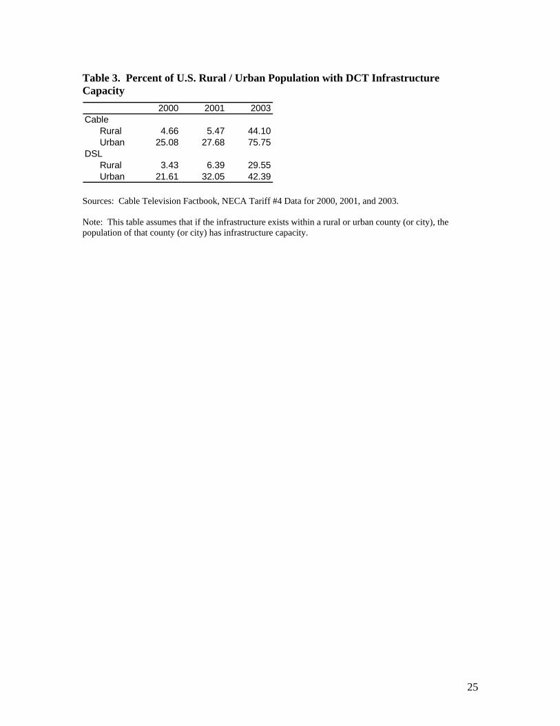
Table 3. Percent of U.S. Rural / Urban Population with DCT Infrastructure Capacity

2000 2001 2003Cable

Rural 4.66 5.47 44.10Urban 25.08 27.68 75.75

DSLRural 3.43 6.39 29.55Urban 21.61 32.05 42.39

Sources: Cable Television Factbook, NECA Tariff #4 Data for 2000, 2001, and 2003.

Note: This table assumes that if the infrastructure exists within a rural or urban county (or city), the population of that county (or city) has infrastructure capacity.

25

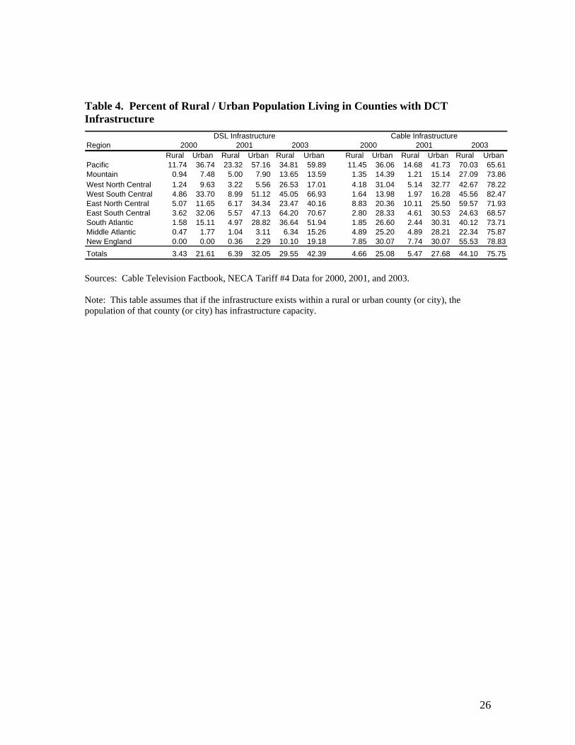
Table 4. Percent of Rural / Urban Population Living in Counties with DCT Infrastructure

DSL Infrastructure Cable InfrastructureRegion 2000 2001 2003 2000 2001 2003

Rural Urban Rural Urban Rural Urban Rural Urban Rural Urban Rural UrbanPacific 11.74 36.74 23.32 57.16 34.81 59.89 11.45 36.06 14.68 41.73 70.03 65.61Mountain 0.94 7.48 5.00 7.90 13.65 13.59 1.35 14.39 1.21 15.14 27.09 73.86West North Central 1.24 9.63 3.22 5.56 26.53 17.01 4.18 31.04 5.14 32.77 42.67 78.22West South Central 4.86 33.70 8.99 51.12 45.05 66.93 1.64 13.98 1.97 16.28 45.56 82.47East North Central 5.07 11.65 6.17 34.34 23.47 40.16 8.83 20.36 10.11 25.50 59.57 71.93East South Central 3.62 32.06 5.57 47.13 64.20 70.67 2.80 28.33 4.61 30.53 24.63 68.57South Atlantic 1.58 15.11 4.97 28.82 36.64 51.94 1.85 26.60 2.44 30.31 40.12 73.71Middle Atlantic 0.47 1.77 1.04 3.11 6.34 15.26 4.89 25.20 4.89 28.21 22.34 75.87New England 0.00 0.00 0.36 2.29 10.10 19.18 7.85 30.07 7.74 30.07 55.53 78.83Totals 3.43 21.61 6.39 32.05 29.55 42.39 4.66 25.08 5.47 27.68 44.10 75.75

Sources: Cable Television Factbook, NECA Tariff #4 Data for 2000, 2001, and 2003.

Note: This table assumes that if the infrastructure exists within a rural or urban county (or city), the population of that county (or city) has infrastructure capacity.

26

Table 5. Logit Model Results for General Internet Access Dependent Variable: access

2000 2001 2003Variable Coefficient S.E. Coefficient S.E. Coefficient S.E.

hs 0.6666 0.0601 *** 0.6135 0.0520 *** 0.6185 0.0510 ***scoll 1.2782 0.0609 *** 1.1423 0.0531 *** 1.2538 0.0528 ***coll 1.5698 0.0658 *** 1.4229 0.0605 *** 1.5520 0.0605 ***collplus 1.7100 0.0734 *** 1.5497 0.0700 *** 1.7105 0.0729 ***faminc1 -0.2491 0.1458 * -0.2217 0.1239 * -0.1569 0.1116 faminc2 -0.1843 0.1458 -0.2127 0.1244 * -0.2470 0.1155 **faminc3 -0.1313 0.1307 0.0698 0.1096 -0.0628 0.1045 faminc4 0.2247 0.1250 * -0.0427 0.1123 -0.0333 0.1072 faminc5 0.2090 0.1114 * 0.0768 0.1001 0.0902 0.0952 faminc6 0.2491 0.1066 ** 0.2972 0.0943 *** 0.2605 0.0915 ***faminc7 0.4869 0.1053 *** 0.4551 0.0946 *** 0.3232 0.0900 ***faminc8 0.6995 0.1058 *** 0.7215 0.0948 *** 0.5116 0.0902 ***faminc9 0.6940 0.1067 *** 0.7317 0.0961 *** 0.7233 0.0936 ***faminc10 0.9629 0.1027 *** 0.9637 0.0926 *** 0.9508 0.0887 ***faminc11 1.1058 0.1042 *** 1.1658 0.0940 *** 1.1027 0.0925 ***faminc12 1.3663 0.1054 *** 1.4011 0.0962 *** 1.3726 0.0933 ***faminc13 1.7264 0.1026 *** 1.8022 0.0931 *** 1.6671 0.0905 ***netatwork 0.0614 0.0389 0.4892 0.0360 *** 0.5325 0.0395 ***black -0.8211 0.0520 *** -0.7439 0.0468 *** -0.6728 0.0482 ***othrace -0.1375 0.0712 * 0.0208 0.0739 -0.1981 0.0704 ***hisp -0.7281 0.0580 *** -0.6885 0.0560 *** -0.6647 0.0524 ***peage 0.0425 0.0062 *** 0.0440 0.0055 *** 0.0606 0.0059 ***age2 -0.0007 0.0001 *** -0.0007 0.0001 *** -0.0008 0.0001 ***sex -0.0018 0.0306 -0.0218 0.0297 0.0118 0.0306married 0.4698 0.0334 *** 0.5798 0.0332 *** 0.5449 0.0339 ***chld1 -0.0793 0.0482 0.2067 0.0435 *** 0.2515 0.0468 ***chld2 -0.0324 0.0490 0.3459 0.0475 *** 0.2992 0.0511 ***chld3 -0.1361 0.0774 * 0.2659 0.0691 *** 0.1913 0.0742 **chld4 0.2424 0.1400 * 0.1515 0.1083 0.1484 0.1313chld5 -0.1259 0.1014 0.0883 0.1918 0.1944 0.2075 regdensity 2.9113 0.2556 *** 2.3981 0.2540 *** 2.3540 0.2799 ***cableacce

s 0.0277 0.0950 -0.1041 0.0869 0.0094 0.0831 dslaccess 0.1078 0.0675 0.0677 0.0596 0.0730 0.0608 retired 0.0114 0.0648 0.0633 0.0576 0.1876 0.0575 ***nm 0.1142 0.0514 ** 0.0352 0.0516 0.0620 0.0541constant -3.9198 0.2059 *** -3.6942 0.2079 *** -3.9747 0.2463 ******, **, and * indicate statistical significance at the p = 0.01, 0.05, and .10 levels, respectively

27

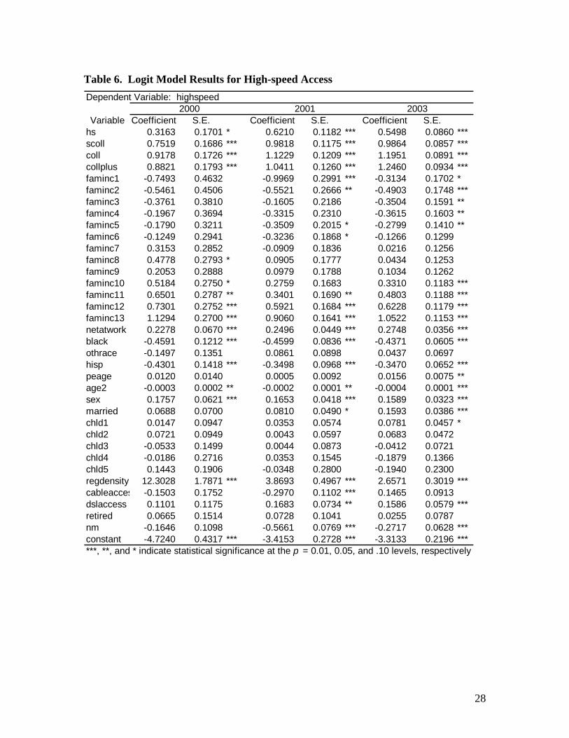
Table 6. Logit Model Results for High-speed Access Dependent Variable: highspeed

2000 2001 2003Variable Coefficient S.E. Coefficient S.E. Coefficient S.E.

hs 0.3163 0.1701 * 0.6210 0.1182 *** 0.5498 0.0860 ***scoll 0.7519 0.1686 *** 0.9818 0.1175 *** 0.9864 0.0857 ***coll 0.9178 0.1726 *** 1.1229 0.1209 *** 1.1951 0.0891 ***collplus 0.8821 0.1793 *** 1.0411 0.1260 *** 1.2460 0.0934 ***faminc1 -0.7493 0.4632 -0.9969 0.2991 *** -0.3134 0.1702 *faminc2 -0.5461 0.4506 -0.5521 0.2666 ** -0.4903 0.1748 ***faminc3 -0.3761 0.3810 -0.1605 0.2186 -0.3504 0.1591 **faminc4 -0.1967 0.3694 -0.3315 0.2310 -0.3615 0.1603 **faminc5 -0.1790 0.3211 -0.3509 0.2015 * -0.2799 0.1410 **faminc6 -0.1249 0.2941 -0.3236 0.1868 * -0.1266 0.1299 faminc7 0.3153 0.2852 -0.0909 0.1836 0.0216 0.1256 faminc8 0.4778 0.2793 * 0.0905 0.1777 0.0434 0.1253 faminc9 0.2053 0.2888 0.0979 0.1788 0.1034 0.1262 faminc10 0.5184 0.2750 * 0.2759 0.1683 0.3310 0.1183 ***faminc11 0.6501 0.2787 ** 0.3401 0.1690 ** 0.4803 0.1188 ***faminc12 0.7301 0.2752 *** 0.5921 0.1684 *** 0.6228 0.1179 ***faminc13 1.1294 0.2700 *** 0.9060 0.1641 *** 1.0522 0.1153 ***netatwork 0.2278 0.0670 *** 0.2496 0.0449 *** 0.2748 0.0356 ***black -0.4591 0.1212 *** -0.4599 0.0836 *** -0.4371 0.0605 ***othrace -0.1497 0.1351 0.0861 0.0898 0.0437 0.0697 hisp -0.4301 0.1418 *** -0.3498 0.0968 *** -0.3470 0.0652 ***peage 0.0120 0.0140 0.0005 0.0092 0.0156 0.0075 **age2 -0.0003 0.0002 ** -0.0002 0.0001 ** -0.0004 0.0001 ***sex 0.1757 0.0621 *** 0.1653 0.0418 *** 0.1589 0.0323 ***married 0.0688 0.0700 0.0810 0.0490 * 0.1593 0.0386 ***chld1 0.0147 0.0947 0.0353 0.0574 0.0781 0.0457 *chld2 0.0721 0.0949 0.0043 0.0597 0.0683 0.0472chld3 -0.0533 0.1499 0.0044 0.0873 -0.0412 0.0721 chld4 -0.0186 0.2716 0.0353 0.1545 -0.1879 0.1366 chld5 0.1443 0.1906 -0.0348 0.2800 -0.1940 0.2300regdensity 12.3028 1.7871 *** 3.8693 0.4967 *** 2.6571 0.3019 ***cableacce

s -0.1503 0.1752 -0.2970 0.1102 *** 0.1465 0.0913 dslaccess 0.1101 0.1175 0.1683 0.0734 ** 0.1586 0.0579 ***retired 0.0665 0.1514 0.0728 0.1041 0.0255 0.0787 nm -0.1646 0.1098 -0.5661 0.0769 *** -0.2717 0.0628 ***constant -4.7240 0.4317 *** -3.4153 0.2728 *** -3.3133 0.2196 ******, **, and * indicate statistical significance at the p = 0.01, 0.05, and .10 levels, respectively

28

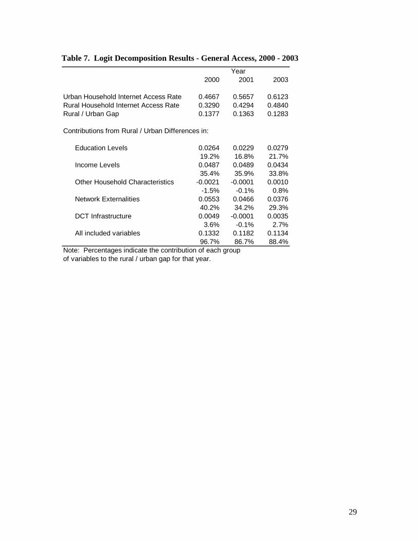
Table 7. Logit Decomposition Results - General Access, 2000 - 2003 Year

2000 2001 2003

Urban Household Internet Access Rate 0.4667 0.5657 0.6123Rural Household Internet Access Rate 0.3290 0.4294 0.4840Rural / Urban Gap 0.1377 0.1363 0.1283

Contributions from Rural / Urban Differences in:

Education Levels 0.0264 0.0229 0.027919.2% 16.8% 21.7%

Income Levels 0.0487 0.0489 0.043435.4% 35.9% 33.8%

Other Household Characteristics -0.0021 -0.0001 0.0010-1.5% -0.1% 0.8%

Network Externalities 0.0553 0.0466 0.037640.2% 34.2% 29.3%

DCT Infrastructure 0.0049 -0.0001 0.00353.6% -0.1% 2.7%

All included variables 0.1332 0.1182 0.113496.7% 86.7% 88.4%

Note: Percentages indicate the contribution of each group of variables to the rural / urban gap for that year.

29

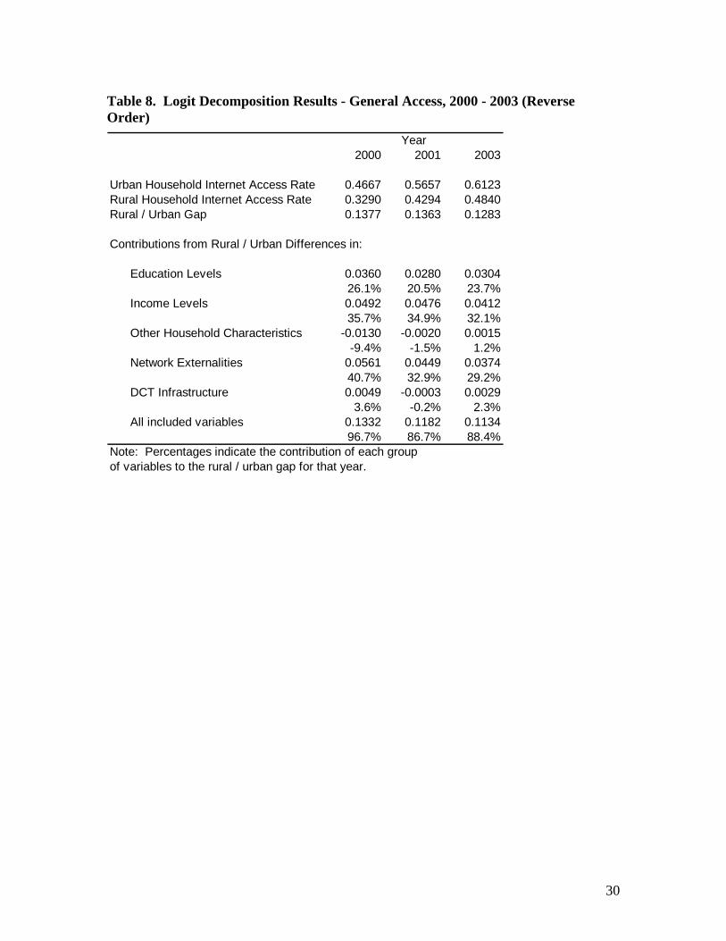
Table 8. Logit Decomposition Results - General Access, 2000 - 2003 (Reverse Order)

Year2000 2001 2003




Income Levels 0.0492 0.0476 0.041235.7% 34.9% 32.1%

Other Household Characteristics -0.0130 -0.0020 0.0015-9.4% -1.5% 1.2%


DCT Infrastructure 0.0049 -0.0003 0.00293.6% -0.2% 2.3%



30

Table 9. Logit Decomposition Results - High-speed Access, 2000 - 2003 Year

2000 2001 2003




Income Levels 0.0081 0.0156 0.031427.1% 20.7% 22.8%

Other Household Characteristics 0.0022 0.0052 0.01037.4% 6.9% 7.5%


DCT Infrastructure -0.0001 -0.0010 0.0084-0.3% -1.3% 6.1%



31

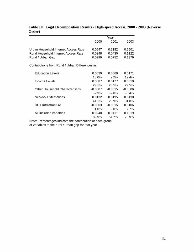
Table 10. Logit Decomposition Results - High-speed Access, 2000 - 2003 (Reverse Order)

Year2000 2001 2003




Income Levels 0.0087 0.0177 0.031029.1% 23.5% 22.5%

Other Household Characteristics -0.0007 -0.0015 -0.0006-2.3% -2.0% -0.4%


DCT Infrastructure -0.0003 -0.0015 0.0106-1.0% -2.0% 7.7%


Notof v

e: Percentages indicate the contribution of each group ariables to the rural / urban gap for that year.

32

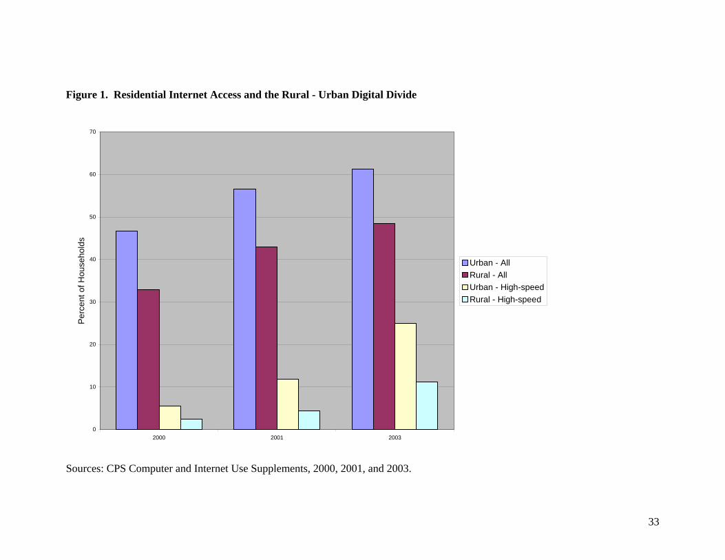
Figure 1. Residential Internet Access and the Rural - Urban Digital Divide

0

10

20

30

40

50

60

70

2000 2001 2003

Per

cent

of H

ouse

hold

s

Urban - AllRural - AllUrban - High-speedRural - High-speed


33

34

Figure 2. Nine Regions of the U.S. and Residential Dial-up and High-Speed Access Rates (By Region)

Dial-up High-speedRegion 2000 2001 2003 2000 2001 2003

Rural Urban Rural Urban Rural Urban Rural Urban Rural Urban Rural UrbanPacific 39.31 48.81 44.20 46.18 42.95 36.47 2.88 6.64 6.12 17.89 16.68 29.46Mountain 39.49 42.21 42.45 47.83 41.38 40.59 1.86 5.09 4.82 9.96 11.33 20.46West North Central 30.30 42.21 39.42 45.48 37.05 36.68 2.29 5.77 4.43 12.64 13.17 27.32West South Central 25.54 33.62 32.80 40.89 33.26 34.14 2.28 5.22 2.30 8.94 8.84 17.33East North Central 33.89 41.28 43.88 46.10 39.68 37.33 2.01 4.20 2.69 8.51 9.15 21.47East South Central 23.50 38.29 30.17 43.12 32.50 34.69 3.61 4.54 5.98 7.05 9.45 20.43South Atlantic 28.92 39.83 36.23 45.73 35.64 37.62 2.42 4.83 3.02 9.62 9.75 22.95Middle Atlantic 39.25 41.57 40.14 44.93 37.85 35.04 3.16 5.14 7.58 12.43 15.40 27.39New England 48.83 43.96 52.11 45.57 45.98 36.01 2.06 7.46 6.73 15.91 17.90 30.95Totals 30.42 41.20 38.64 44.75 37.18 36.22 2.48 5.47 4.30 11.82 11.22 25.01


Pacific

Mountain

West South Central

East South

Central

South Atlantic

West North Central East North

Central

Middle Atlantic

New EnglandPacific

Mountain

West South Central

East South

Central

South Atlantic

West North Central East North

Central

Middle Atlantic

New England

Appendix A

State-level Rates of Dial-up and High-speed Access: 2000, 2001, and 2003

Dial-up High-speed Region

2000 2001 2003 2000 2001 2003Rural Urban Rural Urban Rural Urban Rural Urban Rural Urban Rural Urban

Maine 37.03 37.72 47.12 46.40 44.22 39.90 3.32 9.86 6.49 16.08 14.37 26.64New Hampshire 59.88 46.27 52.90 45.63 41.42 34.49 3.52 8.71 9.90 19.04 24.03 36.39Vermont 45.31 51.72 46.76 49.47 45.12 40.79 1.42 7.00 7.33 17.50 13.53 34.08 New EnglandMassachusetts 53.10 41.16 61.66 42.17 53.17 33.33 0.00 8.40 3.19 15.72 19.66 30.40Rhode Island N/A 35.44 N/A 44.73 N/A 31.22 N/A 5.96 N/A 12.56 N/A 27.96Connecticut N/A 51.46 N/A 45.02 N/A 36.37 N/A 4.85 N/A 14.55 N/A 30.21

New York 36.66 37.46 36.14 41.55 36.52 31.72 5.59 5.38 6.52 14.55 21.42 27.12New Jersey N/A 45.24 N/A 48.94 N/A 35.08 N/A 5.97 N/A 13.42 N/A 31.62 Middle AtlanticPennsylvania 37.85 42.00 44.14 44.31 39.18 38.34 0.73 4.07 8.63 9.34 9.38 23.44

Ohio 32.81 40.25 51.61 44.57 42.87 37.88 1.50 4.91 3.00 9.25 9.17 20.82Indiana 34.10 40.64 40.29 49.08 43.08 40.77 3.67 4.36 2.88 6.58 6.01 14.95Illinois 31.02 42.57 40.25 45.75 34.01 36.51 0.00 3.32 0.59 7.95 11.90 22.09 East North CentralMichigan 41.46 40.12 43.05 43.37 36.32 33.96 2.45 6.13 1.82 11.78 5.78 24.88Wisconsin 30.05 42.83 44.21 47.72 42.14 37.54 2.48 2.29 5.14 7.02 12.90 24.63

Minnesota 27.94 45.18 39.69 53.98 36.75 45.69 3.20 5.62 3.64 9.96 14.21 24.15Iowa 29.02 40.98 42.40 47.19 38.32 42.55 2.60 6.23 6.67 13.24 14.41 25.90Missouri 32.71 41.90 48.01 43.33 35.68 41.30 1.78 7.61 4.67 10.13 7.76 22.39North Dakota 30.82 40.65 39.35 44.16 40.00 31.63 1.42 3.47 1.43 9.51 14.05 25.29 West North CentralSouth Dakota 31.92 40.73 32.79 47.54 30.80 32.48 1.97 4.39 8.57 14.28 19.31 30.85Nebraska 26.70 41.64 30.08 40.37 37.44 34.00 3.97 5.57 3.30 15.76 9.62 31.89Kansas 33.02 44.41 43.65 41.78 40.35 29.07 1.12 7.50 2.71 15.62 12.84 30.75

Delaware 39.29 46.39 38.67 49.97 44.02 43.23 6.19 6.50 1.33 9.70 8.82 19.31Maryland N/A 41.13 N/A 52.00 N/A 41.51 N/A 5.11 N/A 11.20 N/A 24.18DC N/A 36.71 N/A 37.33 N/A 36.83 N/A 4.15 N/A 8.51 N/A 24.24Virginia 30.07 48.02 41.81 52.99 43.18 45.46 0.93 3.50 5.65 8.63 11.19 24.00West Virginia 25.74 37.61 34.83 42.88 35.48 34.97 2.03 5.04 2.48 6.58 10.53 21.61 South AtlanticNorth Carolina 31.04 35.93 31.47 41.14 35.18 32.39 3.93 4.14 5.97 8.90 11.91 24.63South Carolina 25.35 30.48 34.76 41.63 31.32 30.13 0.00 5.21 1.43 10.97 9.90 20.77Georgia 17.90 42.67 28.09 48.39 29.41 36.59 0.92 3.70 3.13 10.07 10.94 25.61Florida 33.08 39.54 44.01 45.26 30.93 37.51 2.95 6.16 1.13 12.03 4.97 22.20

Kentucky 26.35 41.58 42.43 46.44 39.37 45.06 3.72 6.01 2.65 3.91 8.54 19.47Tennessee 23.12 41.28 27.53 40.59 29.11 30.57 3.94 5.23 9.33 11.39 11.61 25.41Alabama 24.37 38.73 23.59 38.49 29.82 32.16 1.24 2.65 4.58 6.66 9.26 19.14 East South CentralMississippi 20.17 31.58 27.12 46.97 31.68 30.98 5.53 4.28 7.36 6.25 8.39 17.71

Arkansas 21.63 29.16 28.81 38.05 28.82 33.07 1.92 2.84 3.53 4.92 13.27 14.61Louisiana 31.62 30.63 38.31 36.29 35.08 34.25 0.94 5.03 1.64 7.46 3.26 14.44Oklahoma 24.45 36.63 30.60 47.98 34.61 34.15 4.44 7.47 2.97 11.58 10.55 17.88 West South CentralTexas 24.47 38.06 33.50 41.23 34.53 35.08 1.84 5.55 1.07 11.79 8.30 22.39

Montana 41.80 38.11 46.90 47.12 40.77 38.90 1.60 4.04 2.74 6.42 9.24 14.90Idaho 38.77 47.25 48.62 45.97 45.88 44.21 1.99 3.75 5.03 13.22 13.39 18.03Wyoming 43.07 45.56 44.03 56.40 44.22 48.04 1.99 1.48 6.76 6.63 13.38 14.41Colorado 40.75 49.05 43.80 50.19 51.08 40.34 2.64 5.89 6.22 11.71 10.00 27.03 MountainNew Mexico 26.84 36.48 31.25 49.73 39.77 42.06 1.41 6.67 2.70 3.18 4.37 10.76Arizona 30.22 40.31 36.37 40.08 32.17 31.76 0.00 7.40 6.55 15.45 16.81 25.87Utah 47.20 46.37 40.91 44.56 39.33 46.65 3.20 5.33 5.38 15.08 14.42 23.84Nevada 47.30 34.56 47.72 48.59 37.84 32.77 2.09 6.20 3.21 8.04 9.01 28.82

Washington 27.23 47.91 42.41 50.58 40.12 36.00 3.63 6.53 1.17 15.89 13.66 32.91Oregon 40.64 56.32 44.71 49.96 44.74 46.27 2.40 3.96 8.30 12.49 12.58 22.53California 42.54 43.48 35.25 44.20 40.93 36.09 4.72 6.51 4.98 15.63 10.50 29.30 PacificAlaska 46.97 55.90 53.79 52.07 50.17 40.60 3.66 7.60 8.85 19.17 19.59 30.31Hawaii 39.15 40.46 44.84 34.09 38.81 23.41 0.00 8.63 7.30 26.29 27.09 32.27

35

Appendix B State-level Rates of DCT Infrastructure Capacity (Cable and DSL)

2000, 2001, and 2003 These numbers represent the percentage of rural / urban population within each state that had DSL or Cable access within their city (for DSL) or county (for Cable) of residence.

DSL Cable2000 2001 2003 2000 2001 2003 Region

Rural Urban Rural Urban Rural Urban Rural Urban Rural Urban Rural UrbanMaine 0.00 0.00 1.07 1.32 6.10 5.76 11.41 15.33 10.76 15.33 57.61 87.92New Hampshire 0.00 0.00 0.00 0.00 6.86 1.46 11.42 32.85 11.42 32.85 71.52 73.16Vermont 0.00 0.00 1.10 5.58 8.01 5.58 0.00 0.00 0.00 0.00 45.68 53.81 New EnglandMassachusetts 0.00 0.00 0.00 6.84 0.00 9.40 0.00 27.19 0.00 27.19 58.39 92.24Rhode Island 0.00 0.00 0.00 0.00 0.00 19.55 0.00 70.80 0.00 70.80 0.00 76.32Connecticut 0.00 0.00 0.00 0.00 39.62 73.32 24.25 34.24 24.25 34.24 100.00 89.56

New York 0.00 2.70 1.67 3.61 7.18 30.44 0.00 13.10 0.00 13.64 12.00 96.78New Jersey 0.00 0.00 0.00 0.00 0.00 3.61 0.00 32.85 0.00 32.85 0.00 73.16 Middle AtlanticPennsylvania 1.40 2.62 1.44 5.72 11.85 11.73 14.68 29.67 14.68 38.16 55.03 57.65

Ohio 13.00 6.90 14.15 26.85 39.63 41.59 4.62 22.01 6.02 22.01 72.97 70.59Indiana 3.13 16.86 5.49 47.80 27.17 61.35 18.51 14.59 18.70 18.65 80.86 56.79Illinois 4.67 32.75 4.67 54.32 12.09 39.20 1.46 22.68 6.13 40.57 25.12 85.79 East North CentralMichigan 4.55 0.68 4.55 18.61 10.26 20.62 18.21 40.42 18.21 45.16 47.57 70.56Wisconsin 0.00 1.03 1.98 24.10 28.20 38.05 1.37 2.11 1.51 1.08 71.35 75.91

Minnesota 0.85 0.00 1.96 5.04 9.38 9.43 5.76 4.03 5.90 4.16 32.32 100.00Iowa 0.07 0.00 0.66 0.74 15.95 9.36 0.44 53.20 3.17 53.84 37.73 73.16Missouri 6.37 19.13 6.36 24.48 33.02 46.69 0.00 3.59 0.07 7.04 18.38 29.13North Dakota 0.00 0.00 1.71 0.00 47.77 1.78 0.52 30.10 0.78 30.10 48.42 87.67 West North CentralSouth Dakota 0.00 0.00 9.07 0.00 28.36 0.79 17.38 42.77 19.13 45.78 59.36 100.00Nebraska 0.00 0.00 1.41 0.00 9.70 1.34 0.00 76.12 0.29 76.23 48.29 81.34Kansas 1.37 48.25 1.37 8.68 41.56 49.65 5.17 7.48 6.64 12.21 54.20 76.24

Delaware 0.00 0.00 0.00 9.48 0.00 9.48 0.00 80.18 0.00 80.18 19.08 90.10Maryland 0.00 0.00 0.00 16.09 0.00 17.48 0.00 40.95 0.00 40.95 41.44 68.52DC 0.00 0.00 0.00 0.00 0.00 100.00 0.00 0.00 0.00 0.00 0.00 100.00Virginia 9.89 15.47 7.51 27.37 45.32 30.77 5.64 31.92 5.64 36.22 23.77 59.52West Virginia 0.00 0.00 0.00 0.33 6.71 39.65 0.00 0.00 0.00 21.34 36.81 61.88 South AtlanticNorth Carolina 0.52 40.50 24.32 67.58 78.47 85.43 1.24 8.17 1.24 8.17 55.07 91.62South Carolina 3.82 24.35 4.33 45.86 59.78 61.44 8.45 15.33 8.45 15.89 93.14 57.68Georgia 0.00 29.08 2.16 51.68 70.86 75.17 1.30 46.11 6.62 46.47 29.74 53.68Florida 0.00 26.61 6.41 41.00 68.58 48.01 0.00 16.75 0.00 23.56 62.04 80.37

Kentucky 7.78 19.20 8.91 35.84 60.90 53.88 0.73 60.14 0.73 60.47 15.67 70.24Tennessee 1.87 54.07 5.90 66.16 70.64 89.30 2.82 39.01 2.82 41.43 26.44 84.14Alabama 3.65 31.97 6.32 49.19 51.51 66.80 3.38 6.72 7.65 8.44 28.36 63.69 East South CentralMississippi 1.16 23.02 1.16 37.35 73.75 72.70 4.26 7.45 7.23 11.78 28.05 56.23

Arkansas 0.00 16.64 7.59 42.40 36.02 67.90 5.60 6.10 5.60 13.32 65.17 100.00Louisiana 3.56 38.63 6.90 52.98 74.39 74.14 0.00 33.47 0.00 34.54 47.30 70.16Oklahoma 0.00 56.88 3.36 50.51 30.91 56.63 0.88 0.00 0.88 0.91 31.18 93.67 West South CentralTexas 15.89 22.63 18.12 58.59 38.88 69.04 0.10 16.33 1.40 16.35 38.59 66.06

Montana 0.00 0.00 14.47 0.00 25.44 26.51 0.49 0.00 0.49 0.00 10.74 55.94Idaho 2.56 5.80 2.56 5.80 8.66 5.80 0.32 0.00 0.32 0.00 49.45 54.01Wyoming 0.00 0.00 0.00 0.00 1.56 0.00 3.56 0.00 3.56 0.00 24.85 92.16Colorado 0.00 0.00 12.81 0.00 26.29 3.73 0.00 13.74 0.00 17.01 4.72 74.34New Mexico 0.00 0.00 0.00 0.00 21.12 0.00 0.00 28.81 0.00 28.81 12.00 70.53 MountainArizona 0.00 0.09 0.00 0.09 8.02 9.49 2.19 0.00 1.10 2.68 48.95 100.00Utah 0.00 0.00 4.44 0.00 12.44 0.44 0.00 2.98 0.00 2.98 0.18 46.37Nevada 4.96 53.97 5.70 57.34 5.70 62.78 4.22 69.61 4.22 69.61 65.79 97.50

Washington 11.09 16.47 25.01 23.60 39.34 27.05 44.51 31.72 44.51 52.32 84.62 73.60Oregon 6.73 16.49 20.93 18.25 40.38 28.46 1.13 29.50 17.27 34.89 77.09 78.41California 11.74 75.68 27.37 83.34 31.88 83.33 10.24 23.02 10.24 25.37 54.35 64.39 PacificAlaska 0.00 0.00 14.15 85.53 33.30 85.53 1.38 0.00 1.38 0.00 100.00 13.19Hawaii 29.16 75.07 29.16 75.07 29.16 75.07 0.00 96.07 0.00 96.07 34.07 98.44

36

Documents

The Role of Infrastructure in the Rural â€“ Urban Digital Divide