The Rural-Urban Divide in India∗

Viktoria Hnatkovska† and Amartya Lahiri‡

June 2012

Abstract

We examine the gaps between rural and urban India in terms of the education attainment,

occupation choices, consumption and wages. We study the period 1983-2010 using household

survey data from successive rounds of the National Sample Survey. We find that this period

has been characterized by a significant narrowing of the differences in education, occupation

distribution, and wages between individuals in rural India and their urban counterparts. We find

that individual characteristics do not appear to account for much of this convergence. Our results

suggest that policy interventions favoring rural areas may have been key in inducing these time

series patterns.

JEL Classification: J6, R2

Keywords: Rural urban disparity, education gaps, wage gaps

∗We would like to thank IGC for a grant funding this research and Arka Roy Chaudhuri for research assistance.†Department of Economics, University of British Columbia, 997 - 1873 East Mall, Vancouver, BC V6T 1Z1, Canada

and Wharton School, University of Pennsylvania. E-mail address: hnatkovs@mail.ubc.ca.‡Department of Economics, University of British Columbia, 997 - 1873 East Mall, Vancouver, BC V6T 1Z1, Canada.

E-mail address: amartyalahiri@gmail.com.

1

1 Introduction

A topic of long running interest to social scientists has been the processes that surround the transfor-

mation of economies along the development path. As is well documented, the process of development

tends to generate large scale structural transformations of economies as they shift from being primar-

ily agrarian towards more industrial and service oriented activities. A related aspect of this trans-

formation is how the workforce in such economies adjusts to the changing macroeconomic structure

in terms of their labor market choices such as investments in skills, choices of occupations, location

and industry of employment. Indeed, some of the more widely cited contributions to development

economics have tended to focus precisely on these aspects. The well known Harris-Todaro model of

Harris and Todaro (1970) was focused on the process through which rural labor migrates to urban

areas in response to wage differentials while the equally venerated Lewis model, formalized in Lewis

(1954), addressed the issue of shifting incentives for employment between rural agriculture and urban

industry.

A parallel literature has addressed the issue of the redistributionary effects associated with these

structural transformations, both in terms of theory and data. The main focus of this research is on

the relationship between development and inequality.1 This work is related to the issue of rural-urban

dynamics since the process of structural transformation implies contracting and expanding sectors

which, in turn, implies a reallocation and, possibly, re-training of the workforce. The capacity of

institutions in such transforming economies to cope with these demands is a fundamental factor that

determines how smooth or disruptive this process is. Clearly, the greater the disruption, the more

the likelihood of income redistributions through unemployment and wage losses due to incompatible

skills.

India over the past three decades has been on exactly such a path of structural transformation.

Prodded by a sequence of reforms starting in the mid 1980s, the country is now averaging annual

growth rates routinely is excess of 8 percent. This is in sharp contrast to the first 40 years since

1947 (when India became an independent country) during which period the average annual output

growth hovered around the 3 percent mark, a rate that barely kept pace with population growth

during this period. This phase has also been marked by a significant transformation in the output

composition of the country with the agricultural sector gradually contracting both in terms of its

1Perhaps the best known example of this line of work is the "Kuznets curve" idea that inequality follows an inverse-U shape with development or income (see Kuznets (1955)). More recent work on this topic explores the relationshipbetween inequality and growth (see, for example, Persson and Tabellini (1994) and Alesina and Rodrik (1994) forillustrative evidence regarding this relationship in the cross-country data).

2

output and employment shares. The big expansion has occurred in the service sector. The industrial

sector has also expanded but at a far lower pace. These patterns of structural transformation since

1983 are shown in Figure 1.

Figure 1: Industry distribution

020

4060

8010

0

1983 1987­88 1993­94 1999­00 2004­05 2007­08

Sectoral employ ment shares

Agri Manuf Serv

020

4060

8010

0

1983 1987­88 1993­94 1999­00 2004­05 2007­08

Sectoral output shares

Agri Manuf Serv

(a) (b)Notes: Panel (a) of this Figure presents the distribution of workforce across three industry categories fordifferent NSS rounds. Panel (b) presents distribution of output (measured in constant 1980-81 prices)across three industry categories. The source for the figure is Hnatkovska and Lahiri (2011).

How has the workforce in rural and urban India responded to these shifting aggregate sectoral

patterns? Have these changes been accompanied by widening rural-urban disparities or have the

disparities between them been shrinking over time? In this paper we address these issues by studying

the evolution of education attainment levels, the occupation choices, the wage and consumption

expenditures of rural and urban workers in India between 1983 and 2010. We do this by using data

from six rounds of the National Sample Survey (NSS) of households in India from 1983 to 2009-10.

We find, reassuringly, that this period has been marked by significant narrowing of the gaps

between rural and urban areas in all of these measures. The shrinking of the rural-urban gaps

have been the sharpest in education attainment and wages, but there have also been important

convergent trends in occupation choices. There has been a significantly faster expansion of blue-

collar jobs (primarily production and service workers) in rural areas, which is surprising given the

usual priors that blue and white collar occupations are mostly centered around urban locations. We

also find some interesting distributional features of the changes in wages and consumption during

this period. Specifically, the rural poor (10th percentile) appeared to have gained relative to the

urban poor whereas the rural rich (the 90th percentile) failed to keep pace with the urban rich.

Our broad conclusion from these results is that the incentives generated by the institutional

3

structure of the country have provided useful signals to the workforce in guiding their choices during

this period. As a result, there has been significant churning at the micro levels of the economy. Some

of the resulting changes have been truly striking with the median wage premium of urban workers

declining from around 100 percent in 1983 to just around 22 percent by 2010. This is a welcome

sign.

There is a large body of work on inequality and poverty in India. A sample of this work can

be found in Banerjee and Piketty (2001), Bhalla (2003), Deaton and Dreze (2002) and Sen and

Himanshu (2005). While some of these studies do examine inequality and poverty in the context of

the rural and urban sectors separately (see Deaton and Dreze (2002) in particular), most of this work

is centered on either measuring inequality (through Gini coeffi cients) or poverty, focused either on

consumption or income alone, and restricted to a few rounds of the NSS data at best. An overview

of this work can be found in Pal and Ghosh (2007). Our study is distinct from this body of work in

that we examine multiple indicators of economic achievement over a 27 year period. This gives us

both a broader view of developments as well as a time-series perspective on post-reform India.

The rest of the paper is organized as follows: the next section presents the data and some sample

statistics. Section 3 presents the main results on changes in the rural-urban gaps as well as the

analysis of the rural employment guarantee reform introduced in India in 2005. The last section

contains concluding thoughts.

2 Data

Our data comes from successive rounds of the National Sample Survey (NSS) of households in India

for employment and consumption. The survey rounds that we include in the study are 1983 (round

38), 1987-88 (round 43), 1993-94 (round 50), 1999-2000 (round 55), 2004-05 (round 61), and 2009-

10 (round 66). Since our focus is on determining the trends in occupations and wages, amongst

other things, we choose to restrict the sample to individuals in the working age group 16-65, who

are working full time (defined as those who worked at least 2.5 days in the week prior to be being

sampled), who are not enrolled in any educational institution, and for whom we have both education

and occupation information. We further restrict the sample to individuals who belong to male-led

households.2 These restrictions leave us with, on average, 140,000 to 180,000 individuals per survey

round.

The sample statistics across the rounds are given in Table 1. The table breaks down the overall

2This avoids households with special conditions since male-led households are the norm in India.

4

patterns by individuals and households and by rural and urban locations. Clearly, the sample is

overwhelmingly rural with about 73 percent of households on average being resident in rural areas.

Rural residents are sightly less likely to be male, more likely to be married, and belong to larger

households than their urban counterparts. Lastly, rural areas have more members of backward castes

as measured by the proportion of scheduled castes and tribes (SC/STs).

Table 1: Sample summary statistics(a) Individuals (b) Households

Urban age male married proportion SC/ST hh size1983 35.03 0.87 0.78 0.26 0.16 5.01

(0.07) (0.00) (0.00) (0.00) (0.00) (0.02)1987-88 35.45 0.87 0.79 0.24 0.15 4.89

(0.06) (0.00) (0.00) (0.00) (0.00) (0.02)1993-94 35.83 0.87 0.79 0.26 0.16 4.64

(0.06) (0.00) (0.00) (0.00) (0.00) (0.02)1999-00 36.06 0.86 0.79 0.28 0.18 4.65

(0.07) (0.00) (0.00) (0.00) (0.00) (0.02)2004-05 36.18 0.86 0.77 0.27 0.18 4.47

(0.08) (0.00) (0.00) (0.00) (0.00) (0.02)2009-10 36.96 0.86 0.79 0.29 0.17 4.27

(0.09) (0.00) (0.00) (0.00) (0.00) (0.02)Rural1983 35.20 0.77 0.81 0.74 0.30 5.42

(0.05) (0.00) (0.00) (0.00) (0.00) (0.01)1987-88 35.36 0.77 0.82 0.76 0.31 5.30

(0.04) (0.00) (0.00) (0.00) (0.00) (0.01)1993-94 35.78 0.77 0.81 0.74 0.32 5.08

(0.05) (0.00) (0.00) (0.00) (0.00) (0.01)1999-00 36.01 0.73 0.82 0.72 0.34 5.17

(0.05) (0.00) (0.00) (0.00) (0.00) (0.01)2004-05 36.56 0.76 0.82 0.73 0.33 5.05

(0.05) (0.00) (0.00) (0.00) (0.00) (0.01)2009-10 37.66 0.77 0.83 0.71 0.34 4.77

(0.08) (0.00) (0.00) (0.00) (0.00) (0.02)Difference1983 -0.17*** 0.11*** -0.04*** -0.48*** -0.15*** -0.41***

(0.09) (0.00) (0.00) (0.00) (0.00) (0.03)1987-88 0.09 0.10*** -0.03*** -0.51*** -0.16*** -0.40***

(0.08) (0.00) (0.00) (0.00) (0.00) (0.02)1993-94 0.04 0.10*** -0.02*** -0.47*** -0.16*** -0.44***

(0.08) (0.00) (0.00) (0.00) (0.00) (0.02)1999-00 0.05 0.13*** -0.04*** -0.45*** -0.16*** -0.52***

(0.08) (0.00) (0.00) (0.00) (0.00) (0.02)2004-05 -0.39*** 0.10*** -0.05*** -0.45*** -0.15*** -0.58***

(0.10) (0.00) (0.00) (0.00) (0.00) (0.03)2009-10 -0.70*** 0.09*** -0.04*** -0.42*** -0.17*** -0.50***

(0.12) (0.00) (0.00) (0.00) (0.01) (0.03)Notes: This table reports summary statistics for our sample. Panel (a) gives thestatistics at the individual level, while panel (b) gives the statistics at the level ofa household. Panel labelled "Difference" reports the difference in characteristics be-tween rural and urban. Standard errors are reported in parenthesis. * p-value≤0.10,** p-value≤0.05, *** p-value≤0.01.

Our focus on full time workers may potentially lead to mistaken inference if there have been

significant differential changes in the patterns of part-time work and/or labor force participation

patterns in rural and urban areas. To check this, Figure 2 plots the urban to rural ratios in labor

force participation rates, overall employment rates, as well as full-time and part-time employment

5

rates. As can be see from the Figure, there was some increase in the relative rural part-time work

incidence between 1987 and 2010. Apart from that, all other trends were basically flat.

Figure 2: Labor force participation and employment gaps

.4.5

.6.7

.8.9

11.

1

1983 1987­88 1993­94 1999­00 2004­05 2009­10

lfp employed full­time part­time

Relative labor market gaps

Note: "lfp" refers to the ratio of labor force participation rate of urban to rural sectors. "employed" refersto the ratio of employment rates for the two groups; while "full-time" and "part-time" are, respectively,the ratios of full-time employment rates and part-time employment rates of the two groups.

3 Rural-Urban Gaps

We now turn to our central goal of uncovering the gaps in the characteristics of the workforce between

rural and urban areas. There are four indicators of primary interest: education attainments levels

of the workforce, the occupation distribution of the workforce, the wage levels of workers and their

consumption levels. We investigate each of them in turn.

3.1 Education

Our first indicator of interest is the education levels of the rural and urban workforce. Education

in the NSS data is presented as a category variable with the survey listing the highest education

attainment level in terms of categories such as primary, middle etc. In order to ease the presentation

we proceed in two ways. First, we construct a variable for the years of education. We do so by

assigning years of education to each category based on a simple mapping: not-literate = 0 years;

literate but below primary = 2 years; primary = 5 years; middle = 8 years; secondary and higher

secondary = 10 years; graduate = 15 years; post-graduate = 17 years. Diplomas are treated similarly

6

depending on the specifics of the attainment level.3 Second, we use the reported education categories

but aggregate them into five broad groups: 1 for illiterates, 2 for some but below primary school, 3

for primary school, 4 for middle, and 5 for secondary and above. The results from the two approaches

are similar. While we use the second method for our econometric specifications since these are the

actually reported data (as opposed to the years series that was constructed by us), we also show

results from the first approach below.

Table 2 shows the average years of education of the urban and rural workforce across the six

rounds in our sample. The two features that emerge from the table are: (a) education attainment

rates as measured by years of education were rising in both urban and rural sectors during this

period; and (b) the rural-urban education gap shrank monotonically over this period. The average

years of education of the urban worker was 164 percent higher than the typical rural worker in 1983

(5.83 years to 2.20 years). This advantage declined to 78 percent by 2009-10 (8.42 years to 4.72

years). To put these numbers in perspective, in 1983 the average urban worker had slightly more

than primary education while the typical rural worker was literate but below primary. By 2009-10,

the average urban worker had about a middle school education while the typical rural worker had

almost reached primary education. While the overall numbers indicate the still dire state of literacy

of the workforce in the country, the movements underneath do indicate improvements over time with

the rural workers improving faster.

Table 2: Education Gap: Years of SchoolingAverage years of education Relative education gap

Overall Urban Rural Urban/Rural1983 3.02 5.83 2.20 2.64***

(0.01) (0.03) (0.01) (0.02)1987-88 3.21 6.12 2.43 2.51***

(0.01) (0.03) (0.01) (0.02)1993-94 3.86 6.85 2.98 2.30***

(0.01) (0.03) (0.02) (0.02)1999-2000 4.36 7.40 3.43 2.16***

(0.02) (0.04) (0.02) (0.02)2004-05 4.87 7.66 3.96 1.93***

(0.02) (0.04) (0.02) (0.01)2009-10 5.70 8.42 4.72 1.78***

(0.03) (0.04) (0.03) (0.01)

Notes: This table presents the average years of education for the overall sample and separately for the urbanand rural workforce; as well as the relative gap in the years of education obtained as the ratio of urban torural education years. Standard errors are in parenthesis.

Table 2, while revealing an improving trend for the average worker, nevertheless masks potentially

important underlying heterogeneity in education attainment by cohort, i.e., variation by the age of3We are forced to combine secondary and higher secondary into a combined group of 10 years because the higher

secondary classification is missing in the 38th and 43rd rounds. The only way to retain comparability across roundsthen is to combine the two categories.

7

the respondent. Panel (a) of Figure 3 shows the relative gap in years of education between the typical

urban and rural worker by age group. There are two key results to note from panel (a): (i) the gaps

have been getting smaller over time for all age groups; (ii) the gaps are smaller for the younger age

groups.

Is the education convergence taking place uniformly across all birth cohorts, or are the changes

mainly being driven by ageing effects? To disentangle the two we compute relative education gaps

for different birth cohorts for every survey year. Those are plotted in panel (b) of Figure 3. Clearly,

almost all of the convergence in education attainments takes place through cross-cohort improve-

ments, with the younger cohorts showing the smallest gaps. Ageing effects are symmetric across

all cohorts, except the very oldest. Most strikingly, the average gap in 2009-10 between urban and

rural workers from the youngest birth cohort (born between 1982 and 1988) has almost disappeared

while the corresponding gap for those born between 1954 and 1960 stood at 150 percent. Clearly,

the declining rural-urban gaps are being driven by declining education gaps amongst the younger

workers in the two sectors.

Figure 3: Education gaps by age groups and birth cohorts

1.5

22.

53

3.5

1983 1987­88 1993­94 1999­00 2004­05 2009­10

16­25 26­35 36­45 46­55 56­65

1.5

22.

53

3.5

1983 1987­88 1993­94 1999­00 2004­05 2009­10

1919­25 1926­32 1933­39 1940­46 1947­531954­60 1961­67 1968­74 1975­81 1982­88

(a) (b)Notes: The figures show the relative gap in the average years of education between the urban and ruralworkforce over time for different for different age groups and birth cohorts.

The time trends in years of education potentially mask the changes in the quality of education.

In particular, they fail to reveal what kind of education is causing the rise in years: is it people

moving from middle school to secondary or is it movement from illiteracy to some education? While

both movements would add a similar number of years to the total, the impact on the quality of

the workforce may be quite different. Further, we are also interested in determining whether the

movements in urban and rural areas are being driven by very different movement in the category of

8

education.

Figure 4: Education distribution0

2040

6080

100

URBAN RURAL

19831987­88

1993­941999­00

2004­052009­10

19831987­88

1993­941999­00

2004­052009­10

Distribution of workforce across edu

Edu1 Edu2 Edu3 Edu4 Edu5

01

23

45

1983 1987­88 1993­94 1999­00 2004­05 2009­10

Gap in workforce distribution across edu

Edu1 Edu2 Edu3 Edu4 Edu5

(a) (b)Notes: Panel (a) of this figure presents the distribution of the workforce across five education categoriesfor different NSS rounds. The left set of bars refers to urban workers, while the right set is for ruralworkers. Panel (b) presents relative gaps in the distribution of urban relative to rural workers across fiveeducation categories. See the text for the description of how education categories are defined (category1 is the lowest education level - illiterate).

Panel (a) of Figure 4 shows the distribution of the urban and rural workforce by education

category. Recall that education categories 1, 2 and 3 are "illiterate", "some but below primary

education" and "primary", respectively. Hence in 1983, 55 percent of the urban labor force and over

80 percent of the rural labor force had primary or below education, reflecting the abysmal delivery

of public services in education in the first 35 years of post-independence India. By 2010, the primary

and below category had come down to 30 percent for urban workers and 50 percent for rural workers.

Simultaneously, the other notable trend during this period is the perceptible increase in the secondary

and above category for workers in both sectors. For the urban sector, this category expanded from

about 30 percent in 1983 to around 50 percent in 2010. Correspondingly, the share of the secondary

and higher educated rural worker rose from just around 5 percent of the rural workforce in 1983 to

about 30 percent in 2010. This, along with the decline in the proportion of rural illiterate workers

from 60 percent to around 25 percent, represent the sharpest and most promising changes in the

past 27 years.

Panel (b) of Figure 4 shows the changes in the relative education distributions of the urban

and rural workforce. For each survey year, the Figure shows the fraction of urban workers in each

education category relative to the fraction of rural workers in that category. Thus, in 1983 the urban

workers were over-represented in the secondary and above category by a factor of 5. Similarly, rural

workers were over-represented in the education category 1 (illiterates) by a factor of 2. Clearly, the

9

closer the height of the bars are to one the more symmetric is the distribution of the two groups in

that category while the further away from one they are, the more skewed the distribution is. As the

Figure indicates, the biggest convergence in the education distribution between 1983 and 2010 was

in categories 4 and 5 (middle and secondary and above) where the bars shrank rapidly. There was

also a convergent trend in category 1 (illiterates) where the bar increased in height towards one over

time. However, this was more muted as compared to the convergence in categories 4 and 5.

While the visual impressions suggest convergence in education, are these trends statistically

significant? We turn to this issue next by estimating ordered multinomial probit regressions of

education categories 1 to 5 on a constant and the rural dummy. The aim is to ascertain the significance

of the difference between rural and urban areas in the probability of a worker belonging to each

category as well as the significance of changes over time in these differences. Table 3 shows the

results.

Table 3: Marginal Effect of rural dummy in ordered probit regression for education categoriesPanel (a): Marginal effects, unconditional Panel (b): Changes

1983 1987-88 1993-94 1999-2000 2004-05 2009-10 83 to 93 93 to 10 83 to 10Edu 1 0.352*** 0.340*** 0.317*** 0.303*** 0.263*** 0.229*** -0.035*** -0.088*** -0.123***

(0.003) (0.002) (0.002) (0.003) (0.003) (0.003) (0.004) (0.004) (0.004)Edu 2 0.003*** 0.010*** 0.021*** 0.028*** 0.037*** 0.044*** 0.018*** 0.023*** 0.041***

(0.001) (0.000) (0.001) (0.001) (0.001) (0.001) (0.001) (0.001) (0.001)Edu 3 -0.047*** -0.038*** -0.016*** -0.001* 0.012*** 0.031*** 0.031*** 0.047*** 0.078***

(0.001) (0.001) (0.000) (0.000) (0.001) (0.001) (0.001) (0.001) (0.001)Edu 4 -0.092*** -0.078*** -0.065*** -0.054*** -0.044*** -0.020*** 0.027*** 0.045*** 0.072***

(0.001) (0.001) (0.001) (0.001) (0.001) (0.001) (0.001) (0.001) (0.001)Edu 5 -0.216*** -0.234*** -0.257*** -0.276*** -0.268*** -0.284*** -0.041*** -0.027*** -0.068***

(0.003) (0.002) (0.003) (0.003) (0.003) (0.004) (0.004) (0.005) (0.005)

N 164979 182384 163132 173309 176968 136826Notes: Panel (a) reports the marginal effects of the rural dummy in an ordered probit regression of education categories 1to 5 on a constant and a rural dummy for each survey round. Panel (b) of the table reports the change in the marginaleffects over successive decades and over the entire sample period. N refers to the number of observations. Standard errorsare in parenthesis. * p-value≤0.10, ** p-value≤0.05, *** p-value≤0.01.

Panel (a) of the Table shows that the marginal effect of the rural dummy was significant for

all rounds and all categories. The rural dummy significantly raised the probability of belonging to

education categories 1 and 2 ("illiterate" and "some but below primary education", respectively)

while it significantly reduced the probability of belonging to categories 4-5. In category 3 the sign on

the rural dummy had switched from negative to positive in 2004-05 and stayed that way in 2009-10.

Panel (b) of Table 3 shows that the changes over time in these marginal effects were also significant

for all rounds and all categories. The trends though are interesting. There are clearly significant

convergent trends for education categories 1, 3 and 4. Category 1, where rural workers were over-

represented in 1983 saw a declining marginal effect of the rural dummy. Categories 3 and 4 (primary

and middle school, respectively), where rural workers were under-represented in 1983 saw a significant

10

increase in the marginal effect of the rural status. Hence, the rural under-representation in these

categories declined significantly. Categories 2 and 5 however were marked by a divergence in the

distribution. Category 2, where rural workers were over-represented saw an increase in the marginal

effect of the rural dummy while in category 5, where they were under-represented, the marginal effect

of the rural dummy became even more negative. This divergence though is not inconsistent with

Figure 4. The figure shows trends in the relative gaps while the probit regressions show trends in

the absolute gaps.

In summary, the overwhelming feature of the data on education attainment gaps suggests a strong

and significant trend toward education convergence between the urban and rural workforce. This is

evident when comparing average years of education, the relative gaps by education category as well

as the absolute gaps between the groups in most categories.

3.2 Occupation Choices

We now turn to our second measure of interest: the occupation choices being made by the workforce

in urban and rural areas. Our interest lies in determining whether the occupation choices being

made in the two sectors are showing some signs of convergence. Clearly, there are some fundamental

differences in the sectoral compositions of rural and urban areas making it unlikely/impossible for

the occupation distributions to converge. However, the country as a whole has been undergoing a

structural transformation with an increasing share of output accruing to services with a corresponding

decline in the output share of agriculture. Are these trends translating into symmetric changes in

the rural and urban occupation distributions? Or, is the expansion of the non-agricultural sector

(broadly defined) restricted to urban areas only?

To examine this issue, we aggregate the reported 3-digit occupation categories in the survey into

three broad occupation categories: white-collar occupations like administrators, executives, man-

agers, professionals, technical and clerical workers; blue-collar occupations such as sales workers,

service workers and production workers; agricultural occupations collecting farmers, fishermen, log-

gers, hunters etc.. Figure 5 shows the distribution of these occupations in urban and rural India

across the survey rounds (Panel (a)) as well as the gap in these distributions between the sectors

(Panel (b)).

The urban and rural occupation distributions have the obvious feature that urban areas have a

much smaller fraction of the workforce in agrarian occupations while rural areas have a miniscule

share of people working in white collar jobs. The crucial aspect though is the share of the workforce

11

Figure 5: Occupation distribution0

2040

6080

100

URBAN RURAL

19831987­88

1993­941999­00

2004­052009­10

19831987­88

1993­941999­00

2004­052009­10

Distribution of workforce across occ

white­collar blue­collar agri

02

46

1983 1987­88 1993­94 1999­00 2004­05 2009­10

Gap in workforce distribution across occ

white­collar blue­collar agri

(a) (b)Notes: Panel (a) of this figure presents the distribution of workforce across three occupation categoriesfor different NSS rounds. The left set of bars refers to urban workers, while the right set is for ruralworkers. Panel (b) presents relative gaps in the distribution of urban relative to rural workers across thethree occupation categories.

in blue collar jobs that pertain to both services and manufacturing. The urban sector clearly has a

dominance of these occupations. Importantly though, the share of blue-collar jobs has been rising

not just in urban areas but also in rural areas. In fact, as Panel (b) of Figure 5 shows, the share of

both white collar and blue collar jobs in rural areas are rising faster than their corresponding shares

in urban areas.

What are the non-farm occupations that are driving the convergence between rural and urban

areas? We answer this question by considering disaggregated occupation categories within the white-

collar and blue-collar jobs. We start with the blue-collar jobs that have shown the most pronounced

increase in rural areas. Panel (a) of Figure 6 presents the break-down of all blue-collar jobs into three

types of occupations. The first group are sales workers, which include manufacturer’s agents, retail

and wholesales merchants and shopkeepers, salesmen working in trade, insurance, real estate, and

securities; as well as various money lenders. The second group are service workers, including hotel

and restaurant staff, maintenance workers, barbers, policemen, firefighters, etc. The third group

consists of production and transportation workers and laborers. This group includes among others

miners, quarrymen, and various manufacturing workers. The main result that jumps out of panel

(a) of Figure 6 is the rapid expansion of blue-collar jobs in the rural sector. The share of rural

population employed in blue-collar jobs has increased from under 18 percent to almost 35 percent

between 1983 and 2010. This increase is in sharp contrast with the urban sector where the population

share of blue-collar jobs remained roughly unchanged at around 60 percent during this period. Most

12

of the increase in blue-collar jobs in the rural sector was accounted for by a two-fold expansion in the

share of sales jobs (from 4 percent in 1983 to almost 8 percent in 2010) and production jobs (from

11 percent in 1983 to 23 percent in 2010). While service jobs in the rural areas expanded as well,

the increase was less dramatic. In the urban sector however, the trends have been quite different:

While service jobs have expanded, albeit weakly, the share of sales and production jobs has actually

declined.

Figure 6: Occupation distribution within blue-collar jobs

020

4060

URBAN RURAL

19831987­88

1993­941999­00

2004­052009­10

19831987­88

1993­941999­00

2004­052009­10

Distribution

sales service production/transport/laborers

01

23

45

1983 1987­88 1993­94 1999­00 2004­05 2009­10

Gap in workforce distribution

sales service production/transport/laborers

(a) (b)Notes: Panel (a) of this figure presents the distribution of workforce within blue-collar jobs for differentNSS rounds. The left set of bars refers to urban workers, while the right set is for rural workers. Panel(b) presents relative gaps in the distribution of urban relative to rural workers across different occupationcategories.

Clearly, such distributional changes should have led to a convergence in the rural and urban

occupation distributions. To illustrate this, panel (b) of Figure 7 presents the relative gaps in

the workforce distribution across various blue-collar occupations. The largest gaps in the sectoral

employment shares were observed in sales and service jobs, where the gap was 4.5 times in 1983. The

distributional changes discussed above have led to a more than two-fold decline in the urban-rural

gap in sales jobs. Similarly, the relative gap in production occupations has fallen by more than 100

percent. In service jobs the relative gap has fallen as well, although the drop was not as pronounced.

Next, we turn to white-collar jobs. Panel (a) of Figure 7 presents the distribution of all white-

collar jobs in each sector into three types of occupations. The first is professional, technical and

related workers. This group includes, for instance, chemists, engineers, agronomists, doctors and

veterinarians, accountants, lawyers and teachers. The second is administrative, executive and man-

agerial workers, which include, for example, offi cials at various levels of the government, as well as

proprietors, directors and managers in various business and financial institutions. The third type of

13

occupations consists of clerical and related workers. These are, for instance, village offi cials, book

keepers, cashiers, various clerks, transport conductors and supervisors, mail distributors and com-

munications operators. The figure shows that administrative jobs is the fastest growing occupation

within the white-collar group in both rural and urban areas. It was the smallest category among

all white-collar jobs in both sectors in 1983, but has expanded dramatically ever since to overtake

clerical jobs as the second most popular occupation among white-collar jobs after professional oc-

cupations. Lastly, the share of professional jobs has also increased while the share of clerical and

related jobs has shrunk in both the rural and urban sectors during the same time.

Have the expansions and contractions in various jobs been symmetric across rural and urban

sectors? Panel (b) of Figure 7 presents relative gaps in the workforce distribution across various

white-collar occupations. The biggest difference in occupation distribution between urban and rural

sectors was in administrative jobs, but the gap has declined more than three-fold between 1983 and

2010. Similarly, the relative gap in clerical and in professional jobs has fallen more than two-fold

over the same period.

Figure 7: Occupation distribution within white-collar jobs

010

2030

40

URBAN RURAL

19831987­88

1993­941999­00

2004­052009­10

19831987­88

1993­941999­00

2004­052009­10

Distribution

professional administrative clerical

02

46

810

1983 1987­88 1993­94 1999­00 2004­05 2009­10

Gap in workforce distribution

professional administrative clerical

(a) (b)Notes: Panel (a) of this figure presents the distribution of workforce within white-collar jobs for differentNSS rounds. The left set of bars refers to urban workers, while the right set is for rural workers. Panel(b) presents relative gaps in the distribution of urban relative to rural workers across different occupationcategories.

Overall, these results suggest that the expansion of rural non-farm sector has led to rural-urban

occupation convergence, contrary to a popular belief that urban growth was deepening the rural-

urban divide in India.

Is this visual image of sharp changes in the occupation distribution and convergent trends statis-

tically significant? To examine this we estimate a multinomial probit regression of occupation choices

14

on a rural dummy and a constant for each survey round. The results for the marginal effects of the

rural dummy are shown in Table 4. The rural dummy has a significantly negative marginal effect on

the probability of being in white-collar and blue-collar jobs, while having significantly positive effects

on the probability of being in agrarian jobs. However, as Panel (b) of the Table indicates, between

1983 and 2010 the negative effect of the rural dummy in blue-collar occupations has declined (the

marginal effect has become less negative) while the positive effect on being in agrarian occupations

has become smaller, with both changes being highly significant. Since there was an initial under-

representation of blue-collar occupations and over-representation of agrarian occupations in rural

sector, these results as indicate an ongoing process of convergence across rural and urban areas in

these two occupation. At the same time, the gap in the share of the workforce in white-collar jobs

between urban and rural areas has widened.

Table 4: Marginal effect of rural dummy in multinomial probit regressions for occupationsPanel (a): Marginal effects, unconditional Panel (b): Changes

1983 1987-88 1993-94 1999-2000 2004-05 2009-10 83 to 93 93 to 10 83 to 10white-collar -0.196*** -0.206*** -0.208*** -0.222*** -0.218*** -0.267*** -0.012*** -0.059*** -0.071***

(0.003) (0.002) (0.003) (0.003) (0.003) (0.004) 0.004 0.005 0.005blue-collar -0.479*** -0.453*** -0.453*** -0.434*** -0.400*** -0.318*** 0.026*** 0.135*** 0.161***

(0.003) (0.003) (0.003) (0.004) (0.004) (0.005) 0.004 0.006 0.006agri 0.675*** 0.659*** 0.661*** 0.655*** 0.619*** 0.585*** -0.014*** -0.076*** -0.090***

(0.002) (0.002) (0.002) (0.002) (0.003) (0.003) 0.003 0.004 0.004

N 164979 182384 163132 173309 176968 133926Note: Panel (a) of the table present the marginal effects of the rural dummy from a multinomial probit regression of occupationchoices on a constant and a rural dummy for each survey round. Panel (b) reports the change in the marginal effects of the ruraldummy over successive decades and over the entire sample period. N refers to the number of observations. Agrarian jobs is thereference group in the regressions. Standard errors are in parenthesis. * p-value≤0.10, ** p-value≤0.05, *** p-value≤0.01.

3.3 Wages

The next point of interest is the behavior of wages in urban and rural India. Wages are obtained as

the daily wage/salaried income received for the work done by respondents during the previous week

(relative to the survey week). Wages can be paid in cash or kind, where the latter are evaluated

at the current retail prices. We convert wages into real terms using state-level poverty lines that

differ for rural and urban sectors. We express all wages in 1983 rural Maharashtra poverty lines.4

4 In 2004-05 the Planning Commission of India has changed the methodology for estimation of poverty lines. Amongother changes, they switched from anchoring the poverty lines to a calorie intake norm towards consumer expendituresmore generally. This led to a change in the consumption basket underlying poverty lines calculations. To retaincomparability across rounds we convert 2009-10 poverty lines obtained from the Planning Commission under the newmethodology to the old basket using 2004-05 adjustment factor. That factor was obtained from the poverty lines underthe old and new methodologies available for 2004-05 survey year. As a test, we used the same adjustment factor toobtain the implied "old" poverty lines for 1993-94 survey round for which the two sets of poverty lines are also availablefrom the Planning Commission. We find that the actual old poverty lines and the implied "old" poverty lines are verysimilar, giving us confidence that our adjustment is valid.

15

Importantly, we are interested not just in the mean or median wage gaps, but rather in the behavior

of the wage gap across the entire wage distribution.

In order to present the results, we break up our sample into two sub-periods: 1983 to 2004-05 and

2004-05 to 2009-10. We do this to distinguish long run trends since 1983 from the potential effects of

The Mahatma Gandhi National Rural Employment Guarantee Act (NREGA) that was introduced

in 2005. NREGA provides a government guarantee of a hundred days of wage employment in a

financial year to all rural household whose adult members volunteer to do unskilled manual work.

This Act could clearly have affected rural and urban wages. To control for the effects of this policy

on real wages, we split our sample period into the pre- and post-NREGA periods.

We begin with the pre-NREGA period of 1983 to 2004-05. Panel (a) of Figure 8 plots the kernel

densities of log wages for rural and urban workers for the 1983 and 2004-05 survey rounds. The plot

shows a very clear rightward shift of the wage density function during this period for rural workers.

The shift in the wage distribution for urban workers is much more muted. In fact, the mean almost

did not change, and most of the changes in the distribution took place at the two ends. Specifically,

a fat left tail in the urban wage distribution in 1983, indicating a large mass of urban labor having

low real wages, has disappeared and was replaced by a fat right tail.

Figure 8: The log wage distributions of urban and rural workers for 1983 and 2004-05

0.2

.4.6

.8de

nsity

0 1 2 3 4 5log wage  (real)

Urban ­ 1983 Rural  ­ 1983Urban ­ 2004­05 Rural  ­ 2004­05

­.3­.2

­.10

.1.2

.3.4

.5.6

.7.8

lnw

age(

Urb

an)­

lnw

age(

Rur

al)

0 10 20 30 40 50 60 70 80 90 100percent ile

1983 2004­05

(a) (b)Notes: Panel (a) shows the estimated kernel densities of log real wages for urban and rural workers, whilepanel (b) shows the difference in percentiles of log-wages between urban and rural workers plotted againstthe percentile. The plots are for 1983 and 2004-05 NSS rounds.

Panel (b) of Figure 8 presents the percentile (log) wage gaps between urban and rural workers for

1983 and 2004-05. The plots give a sense of the distance between the urban and rural wage densities

functions in those two survey rounds. An upward sloping gap schedule indicates that wage gaps are

16

rising for richer wage groups. A rightward shift in the schedule over time implies that the wage gap

has shrunk. The plot for 2004-05 lies to the right of that for 1983 till the 70th percentile indicating

that for most of the wage distribution, the gap between urban and rural wages has declined over this

period. Indeed, it is easy to see from Panel (b) that the median log wage gap between urban and

rural wages fell from around 0.7 to around 0.2. Hence, the median wage premium of urban workers

declined from around 100 percent to 22 percent. Between the 70th and 90th percentiles however, the

wage gaps are larger in 2004-05 as compared to 1983. This is driven by the emergence of a large mass

of people in the right tail of the urban wage distribution in 2004-05 period, as we discussed above.

A last noteworthy feature is that in 2004-05, for the bottom 15 percentiles of the wage distribution

in the two sectors, rural wages were actually higher than urban wages. This was in stark contrast to

the picture in 1983 when urban wages were higher than rural wages for all percentiles.

Next we turn to the analysis of the post-NREGA wage distributions. Figure 9 contrasts the

real wage densities of rural and urban workers in 2004-05 and 2009-10. The figure shows that the

urban-rural wage convergence we uncovered for 1983-2005 period continued in the post-reform period

as well. Panel (a) indicates a clear rightward shift in the urban wage distribution, while panel (b)

shows that the percentile gaps in 2009-10 lie to the right and below the gaps for 2004-05 period for

up to 80th percentile.

Figure 9: The log wage distributions of urban and rural workers for 2004-05 and 2009-10

0.2

.4.6

.81

dens

ity

0 1 2 3 4 5log wage  (real)

Urban ­ 2004­05 Rural  ­ 2004­05Urban ­ 2009­10 Rural  ­ 2009­10

­.3­.2

­.10

.1.2

.3.4

.5.6

.7.8

lnw

age(

Urb

an)­

lnw

age(

Rur

al)

0 10 20 30 40 50 60 70 80 90 100percent ile

2004­05 2009­10

(a) (b)Notes: Panel (a) shows the estimated kernel densities of log real wages for urban and rural workers, whilepanel (b) shows the difference in percentiles of log-wages between urban and rural workers plotted againstthe percentile. The plots are for 2004-05 and 2009-10 NSS rounds.

Figures 8 and 9 suggest wage convergence between rural and urban areas. But is this borne out

statistically? To test for this, we estimate Recentered Influence Function (RIF) regressions developed

17

by Firpo, Fortin, and Lemieux (2009) of the log real wages of individuals in our sample on a constant,

controls for age (we include age and age squared of each individual) and a rural dummy for each

survey round. Our interest is in the coeffi cient on rural dummy. The controls for age are intended

to flexibly control for the fact that wages are likely to vary with age and experience. We perform

the analysis for different unconditional quantiles as well as the mean of the wage distribution.5

Table 5: Wage gaps and changesPanel (a): Rural dummy coeffi cient Panel (b): Changes

1983 1993-94 1999-2000 2004-05 2009-10 83 to 94 94 to 10 83 to 1010th quantile -0.208*** -0.031*** -0.013 0.017 0.087*** 0.177*** 0.118*** 0.295***

(0.010) (0.009) (0.008) (0.012) (0.014) (0.013) (0.017) (0.017)50th quantile -0.586*** -0.405*** -0.371*** -0.235*** -0.126*** 0.181*** 0.279*** 0.460***

(0.009) (0.008) (0.008) (0.009) (0.009) (0.012) (0.012) (0.013)90th quantile -0.504*** -0.548*** -0.700*** -0.725*** -1.135*** -0.044*** -0.587*** -0.631***

(0.014) (0.017) (0.024) (0.028) (0.038) (0.022) (0.042) (0.040)mean -0.509*** -0.394*** -0.414*** -0.303*** -0.270*** 0.115*** 0.124*** 0.239***

(0.008) (0.009) (0.010) (0.010) (0.011) (0.012) (0.014) (0.014)

N 63981 63366 67322 64359 57440Note: Panel (a) of this table reports the estimates of coeffi cients on the rural dummy from RIF regressions of log wages on ruraldummy, age, age squared, and a constant. Results are reported for the 10th, 50th and 90th quantiles. Row labelled "mean"reports the rural coeffi cient from the conditional mean regression. Panel (b) reports the changes in the estimated coeffi cientsover successive decades and the entire sample period. N refers to the number of observations. Standard errors are in parenthesis.* p-value≤0.10, ** p-value≤0.05, *** p-value≤0.01.

Panel (a) of Table 5 reports the estimated coeffi cient on the rural dummy for the 10th, 50th and

90th percentiles as well as the mean for different survey rounds.6 Clearly, rural status significantly

reduced wages for almost all percentiles of the distribution across the rounds. However, the size of

the negative rural effect has become significantly smaller over time for the 10th and 50th percentiles

as well as the mean over the entire period as well all sub-periods within (see Panel (b)) with the

largest convergence having occurred for the median. In fact, the coeffi cient on the rural dummy for

the 10th percentile has turned positive, indicating a gap in favor of the rural poor. At the same

time, for the 90th percentile the wage gap actually increased over time. These results corroborate

the visual impression from Figure 8: the wage gap between rural and urban areas fell between 1983

and 2005 for all but the richest wage groups.

While the wage convergence for most of the distribution is interesting, what were the factors

driving this convergence? We turn to this issue next. Our focus is on two aspects of the wage gaps:

Was the wage convergence documented above driven by a convergence of measured covariates of

5We use the RIF approach (developed by Firpo, Fortin, and Lemieux (2009)) because we are interested in estimatingthe effect of the rural dummy for different points of the distribution, not just the mean. However, since the law ofiterated expectations does not go through for quantiles, we cannot use standard regression methods to determine theunconditional effect of rural status on wages for different quantiles. The RIF methodology essentially gets around thisproblem for quantiles. Details regarding this method can be found in Firpo, Fortin, and Lemieux (2009).

6Due to an anomalous feature of missing rural wage data for 1987-88, we chose to drop 1987-88 from the study ofwages in order to avoid spurious results.

18

wages; or was it due to changes in unmeasured factors? We proceed with two approaches. Our first

approach is to use the procedure developed by DiNardo, Fortin, and Lemieux (1996) (DFL from

hereon) to decompose the overall difference in the observed wage distributions of urban and rural

labor within a sample round into two components — the part that is explained by differences in

attributes and the part that is explained by differences in the wage structure of the two groups. To

obtain the explained part, for each set of attributes we construct a counterfactual density for urban

workers by assigning them the rural distribution of the attributes.7 ,8

We consider several sets of attributes. First, we evaluate the role of individual demographic char-

acteristics such as age, age squared, a dummy for the caste group (SC/ST or not) and a geographic

zone of residence. The latter are constructed by grouping all Indian states into six regions —North,

South, East, West, Central and North-East. Note that we control for caste by including a dummy for

whether or not the individual is an SC/ST in order to account for the fact that SC/STs tend to be

disproportionately rural. Given that they are also disproportionately poor and have little education,

controlling for SC/ST status is important in order to determine the independent effect of rural status

on wages. Second, we add education to the set of attributes and obtain the incremental contribution

of education to the observed wage convergence. Lastly, we evaluate the role played by occupation

differences in the urban-rural wage convergence. Figure 10 presents our findings for the pre-NREGA

period —for 1983 (panel (a)) and 2004-05 (panel (b)). The solid line shows the actual urban-rural

(log) wage gaps for the entire wage distribution, while the broken lines show the gaps explained by

differences in attributes of the two groups, where we introduced the attributes sequentially.

Figure 10 shows that demographic characteristics explain a small fraction of the urban-rural wage

gap. Moreover, this fraction remains stable at around 0.1 along the entire distribution in both 1983

and 2004-05. For the 1983 wage distribution gap, differences in education account for almost entire

wage gap at the bottom of the distribution, while differences in occupation explain the wage gap

for the upper 50 percent of the distribution. Turning to 2004-05 however, the picture is different.

Here differences in education attainments between urban and rural workers explain a large fraction

of the gap at the top end of the distribution (median and above). However, for the bottom end

7The DFL method involves first constructing a counterfactual wage density function for urban individuals by givingthem the attributes of rural households. This is done by a suitable reweighting of the estimated wage density function ofurban households. The counterfactual density is then compared with the actual wage density to assess the contributionof the measured attributes to the observed wage gap.

8We choose to do the reweighting this way to avoid a common support problem, i.e., there may not be enough ruralworkers at the top end of the distribution to be able to mimic the urban distribution.

19

Figure 10: Decomposition of Urban-Rural wage gaps for 1983 and 2004-05­.3

­.2­.1

0.1

.2.3

.4.5

.6.7

.8ln

wag

e(U

rban

)­ln

wag

e(R

ural

)

0 10 20 30 40 50 60 70 80 90 100percentile

actual explained:demogrexplained:edu explained:occ

Urban­Rural wage gap, 1983

­.3­.2

­.10

.1.2

.3.4

.5.6

.7.8

lnw

age(

Urb

an)­

lnw

age(

Rur

al)

0 10 20 30 40 50 60 70 80 90 100percentile

actual explained:demogrexplained:edu explained:occ

Urban­Rural wage gap, 2004­05

(a) (b)Notes: Each panel shows the actual log wage gap between urban and rural workers for each percentile, andthe counterfactual percentile log wage gaps when urban workers are sequentially given rural attributes.Three sets of attributes are considered: demographic (denoted by "demogr"), demographics plus educa-tion ("edu"), and all of the above plus occupations ("occ"). The left panel shows the decomposition for1983 while the right panel is for 2004-05.

of the distribution the education differences suggest that there should exist a large gap in favor of

urban workers. This finding is particularly striking given that wages of rural workers are in fact

higher than wages of urban workers for the bottom 15 percent of distribution, which is the opposite

of what their demographic characteristics and education endowments predict. Adding occupations

deepen the puzzle further. Based on differences in occupations, the urban-rural gap should be more

than 0.2 higher than the actual gap in the data. These results suggest that differences in the wage

structure of the urban and rural workers play an important role in our data.

We conduct an analogous decomposition of the urban-rural wage gap in the post-reform period

of 2009-10. As can be seen from Figure 11 the contribution of various factors in that round resembles

closely our findings for 2004-05. We assess the role played by the reform using state-level variation

in wage gaps in Section 3.5.

Our second approach aims to understand the time-series evolution of wage gaps between urban

and rural workers. We proceed with an adaptation of the Oaxaca-Blinder decomposition technique to

decompose the observed changes in the mean and quantile wage gaps into explained and unexplained

components as well as to quantify the contribution of the key individual covariates. We employ OLS

regressions for the decomposition at the mean, and the RIF regressions for decompositions at the

10th, 50th, and 90th quantiles.9

9All decompositions are performed using a pooled model across rural and urban sectors as the reference model.Following Fortin (2006) we allow for a group membership indicator in the pooled regressions. We also used 1983 round

20

Figure 11: Decomposition of Urban-Rural wage gaps for 2009-10

­.3­.2

­.10

.1.2

.3.4

.5.6

.7.8

lnw

age(

Urb

an)­

lnw

age(

Rur

al)

0 10 20 30 40 50 60 70 80 90 100percentile

actual explained:demogrexplained:edu explained:occ

Urban­Rural wage gap, 2009­10

Notes: This figure shows the actual log wage gap between urban and rural workers for each percentile in2009-10, and the counterfactual percentile log wage gaps when urban workers are sequentially given ruralattributes. Three sets of attributes are considered: demographic (denoted by "demogr"), demographicsplus education ("edu"), and all of the above plus occupations ("occ").

Our set of explained factors, as before, includes demographic characteristics such as individual’s

age, age squared, caste, and geographic region of residence. Additionally, we control for the education

level of the individual by including dummies for education categories 1-5.

Table 6: Decomposing changes in rural-urban wage gaps over time(a). Change 1983 to 2009-10 explained

(i) measured gap (ii) explained (iii) unexplained (iv) education10th quantile -0.371*** -0.096*** -0.275*** -0.059***

(0.036) (0.016) (0.040) (0.013)50th quantile -0.568*** -0.202*** -0.366*** -0.166***

(0.022) (0.014) (0.019) (0.012)90th quantile 0.332*** 0.229*** 0.103*** 0.284***

(0.041) (0.046) (0.045) (0.044)mean -0.263*** -0.115*** -0.148*** -0.078***

(0.019) (0.014) (0.017) (0.012)(b). Change in explained component10th quantile -0.096*** -0.060*** -0.036*** -0.049***

(0.016) (0.008) (0.013) (0.006)50th quantile -0.202*** -0.064*** -0.137*** -0.052***

(0.014) (0.012) (0.014) (0.009)90th quantile 0.229*** 0.060*** 0.169*** 0.084***

(0.046) (0.021) (0.040) (0.020)mean -0.115*** -0.032*** -0.083*** -0.015

(0.014) (0.012) (0.008) (0.010)

Note: Panel (a) presents the change in the rural-urban wage gap between 1983 and 2009-10. Panel (b) reports thedecomposition of the time-series change in the explained component of the change in the wage gap over 1983-2010 period.All gaps are decomposed into explained and unexplained components using the RIF regression approach of Firpo, Fortin,and Lemieux (2009) for the 10th, 50th and 90th quantiles. Both panels also report the contribution of education to theexplained gaps. Bootstrapped standard errors are in parenthesis. * p-value≤0.10, ** p-value≤0.05, *** p-value≤0.01.

Table 6 shows the results of the decomposition exercise. Panel (a) shows the decomposition of

as the benchmark sample. Details of the decomposition method can be found in the Appendix A.1.

21

the measured gap (column (i)) into the explained and unexplained components (columns (ii) and

(iii)), as well as the part of the gap that is explained by education alone (column (iv)). The results

indicate that the majority of the change in the urban-rural wage gap is unexplained for the 10th

percentile and the median. For the 90th percentile most of the change in the wage gap is explained.

The change in the mean wage gap is roughly split between explained and unexplained components.

At all points of the distribution the majority of the explained component is captured by education

attainments.

If the explained component of a regression is βX, then changes in that component has two

components: the change in X and the change β, which is the measured return to X. Since X

is measured in the data, the part of the change in the explained component that is due to X is

"explained" by the data while the part due to β is not directly explained. Panel (b) of the Table 6

decomposes changes in the explained component itself into the explained and unexplained parts. For

the 10th percentile, most of the change in the measured component of the gap was due to changes in

the explained part (or X). For the median and the 90th percentile however, most of the change in

the explained component was due to changes in returns rather than changes in the component itself.

Overall, our conclusion from the wage data is that wages have converged significantly between

rural and urban India during since 1983 for all except the very top of the income distribution.

Education and occupation has been an important contributor to these convergent patterns. However,

a large fraction of the trend is due to unmeasured factors.

3.4 Consumption

Our last indicator of interest is the household expenditure on consumption in rural and urban India.

This measure is the one that is often used in studies on poverty and inequality. The variable we

use is monthly per capita household consumption expenditure, or "mpce". This variable is collected

at the level of the household. We convert consumption expenditures into real terms using offi cial

state-poverty lines, with rural Maharashtra in 1983 as the base — same as we did for wages. In

order to make real consumption results comparable with the wage data, we convert consumption

into per-capita daily value terms.

We start by plotting the kernel densities of the (log) per capita real consumption (we will use

mpce and consumption interchangeably from hereon) for rural and urban households for 1983 and

2004-05 in Panel (a) of Figure 12. Panel (b) of the Figure plots the percentile gaps in (log) per capita

log household consumption between urban and rural households for these two survey rounds.

22

Figure 12: The log consumption distributions of urban and rural households for 1983 and 2004-050

.2.4

.6.8

1de

nsity

­2 0 2 4 6log consumption (real)

Urban ­ 1983 Rural ­ 1983Urban ­ 2004­05 Rural ­ 2004­05

­.10

.1.2

.3.4

.5ln

mpc

e(U

rban

)­ln

mpc

e(R

ural

)

0 10 20 30 40 50 60 70 80 90 100percentile

1983 2004­05

(a) (b)Notes: Panel (a) shows the estimated kernel densities of log per capita real consumption expenditurefor urban and rural households, while panel (b) shows the difference in percentiles of log-consumptionbetween urban and rural households plotted against the percentile. The plots are for the 1983 and 2004-05NSS rounds.

Panel (a) of Figure 12 shows that the consumption distribution shifted to the right for both rural

and urban households during this period. Panel (b) of the figure, which plots the gaps for each

percentile however shows several interesting features. First, consumption gaps in both 1983 and

2004-05 are positive and upward sloping. Second, the plot for 2004-05 is significantly steeper than

the schedule for 1983. Effectively, the consumption gaps between urban and rural areas declined

for percentiles below the median of the consumption distribution but widened above the median.

Interestingly, rural households till around the 30th percentile actually consumed more than their

counterparts in urban areas in 2004-05 (the gaps were negative) whereas the gaps were positive in

1983. Thus, the rural poor have clearly done better than the urban poor during this period, as

measured by their household consumption levels.10 This is an interesting finding in its own right

and may indicate the effects of weaker social and family insurance mechanisms in urban areas for

the poor which leads them to possibly consume less than they would otherwise. This channel has

been suggested as a rationalization for low inequality and mobility in rural India by Munshi and

Rosenzweig (2009).

Next, we consider the post-NREGA period. Panel (a) of Figure 13 contrasts densities of the (log)

per capita real consumption expenditures in the rural and urban sectors for 2004-05 and 2009-10;

while panel (b) reports the percentile gaps in the two periods. Clearly, the trends we uncovered in the

10Note that these findings are similar in nature to the results we obtained for wages though the specifics are different.In particular, for wages the gap shrank for a much larger portion of the distribution than the corresponding narrowingof expenditure gaps in 2004-05.

23

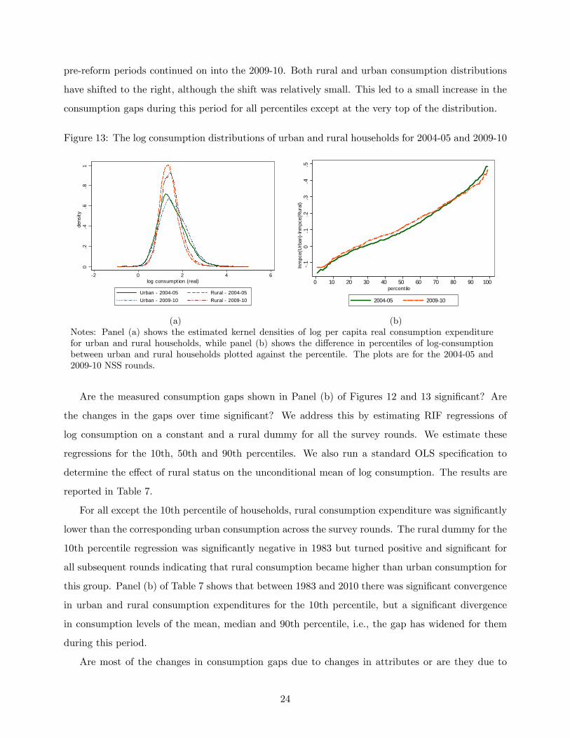
pre-reform periods continued on into the 2009-10. Both rural and urban consumption distributions

have shifted to the right, although the shift was relatively small. This led to a small increase in the

consumption gaps during this period for all percentiles except at the very top of the distribution.

Figure 13: The log consumption distributions of urban and rural households for 2004-05 and 2009-10

0.2

.4.6

.81

dens

ity

­2 0 2 4 6log consumption (real)

Urban ­ 2004­05 Rural ­ 2004­05Urban ­ 2009­10 Rural ­ 2009­10

­.10

.1.2

.3.4

.5ln

mpc

e(U

rban

)­ln

mpc

e(R

ural

)

0 10 20 30 40 50 60 70 80 90 100percentile

2004­05 2009­10

(a) (b)Notes: Panel (a) shows the estimated kernel densities of log per capita real consumption expenditurefor urban and rural households, while panel (b) shows the difference in percentiles of log-consumptionbetween urban and rural households plotted against the percentile. The plots are for the 2004-05 and2009-10 NSS rounds.

Are the measured consumption gaps shown in Panel (b) of Figures 12 and 13 significant? Are

the changes in the gaps over time significant? We address this by estimating RIF regressions of

log consumption on a constant and a rural dummy for all the survey rounds. We estimate these

regressions for the 10th, 50th and 90th percentiles. We also run a standard OLS specification to

determine the effect of rural status on the unconditional mean of log consumption. The results are

reported in Table 7.

For all except the 10th percentile of households, rural consumption expenditure was significantly

lower than the corresponding urban consumption across the survey rounds. The rural dummy for the

10th percentile regression was significantly negative in 1983 but turned positive and significant for

all subsequent rounds indicating that rural consumption became higher than urban consumption for

this group. Panel (b) of Table 7 shows that between 1983 and 2010 there was significant convergence

in urban and rural consumption expenditures for the 10th percentile, but a significant divergence

in consumption levels of the mean, median and 90th percentile, i.e., the gap has widened for them

during this period.

Are most of the changes in consumption gaps due to changes in attributes or are they due to

24

Table 7: Consumption gaps and changesPanel (a): Rural dummy coeffi cient

1983 1987-88 1993-94 1999-00 2004-05 2009-1010th quantile -0.039*** 0.049*** 0.009 0.020** 0.080*** 0.070***

(0.008) (0.008) (0.007) (0.008) (0.009) (0.011)50th quantile -0.066*** -0.039*** -0.088*** -0.096*** -0.072*** -0.091***

(0.007) (0.006) (0.005) (0.006) (0.007) (0.009)90th quantile -0.164*** -0.179*** -0.290*** -0.355*** -0.413*** -0.411***

(0.011) (0.010) (0.011) (0.012) (0.015) (0.018)mean -0.085*** -0.054*** -0.115*** -0.134*** -0.119*** -0.131***

(0.006) (0.005) (0.005) (0.006) (0.007) (0.008)

N 87335 93701 87098 88620 90838 75123Panel (b): Changes

1983 to 1993-94 1993 to 2009-10 1983 to 2009-1010th quantile 0.048*** 0.061*** 0.109***

(0.011) (0.013) (0.014)50th quantile -0.022*** -0.003 -0.025***

(0.009) (0.010) (0.011)90th quantile -0.126*** -0.121*** -0.247***

(0.016) (0.021) (0.021)mean -0.030*** -0.016* -0.046***

(0.008) (0.009) (0.010)

Note: Panel (a) reports the estimates of the coeffi cient on the rural dummy from RIF regressions of log consumptionexpenditures on rural dummy and a constant. Panel (b) reports the changes in the estimated coeffi cients over successivedecades and the entire sample period. N refers to the number of observations. Standard errors are in parenthesis. *p-value≤0.10, ** p-value≤0.05, *** p-value≤0.01.

changes in the consumption structure, i.e., are they due to changes in the X ′s or the β′s? We address

this question with DFL decompositions. Figure 14 reports the actual log consumption gap for urban

labor relative to rural computed for every percentile (solid line); and the explained gaps, computed as

the difference between the actual and reweighted urban consumption percentiles, where we reweighted

the consumption distribution of urban workers by assigning them rural attributes. As with wages,

we examine the influence of individual covariates by introducing them sequentially. We first consider

demographic characteristics, which include household size, the number of earning members of the

household, caste dummy and regional dummies. Then we introduce education attainments, which

consist of the education attainments of the household head and the highest level of education attained

in the household. Lastly, we add occupation dummies for the household head.

Panel (a) shows the results for 1983, while panel (b) reports them for the pre-NREGA period of

2004-05. Our findings are similar of those for wages. Demographic characteristics contribute roughly

0.1 to the observed consumption gaps. In 1983 this explains almost the entire gap at the bottom end

of the distribution (up to the median). In 2004-05 demographics loose their explanatory power. In

fact, the gap predicted by the demographics remains flat for the entire distribution, while the actual

consumption gap is clearly upward sloping. Furthermore, the actual gap is negative at the bottom

end of the distribution, while demographics predict a positive gap in the order of about 0.1. Adding

25

education and occupations to the set of attributes deepens the puzzle: based on the differences in

education attainments and occupation distributions, the consumption gap between urban and rural

workers should be in the order of 0.15-0.2 at the bottom end of the distribution and in the order

of 0.3 at the top end in 1983. The actual gap is significantly smaller. Similarly, in 2004-05 the

actual gaps are orders of magnitude smaller than the gap implied by the differences in attributes,

especially at the lower end of the distribution. Clearly, there is a large unexplained component that

is responsible for the observed consumption gaps, especially when it comes to poor households.

Figure 14: Decomposition of Urban-Rural consumption gaps for 1983 and 2004-05

­.10

.1.2

.3.4

.5ln

mpc

e(U

rban

)­ln

mpc

e(R

ural

)

0 10 20 30 40 50 60 70 80 90 100percentile

actual explained:demogrexplained:edu explained:occ

Urban­Rural consumption gap, 1983

­.10

.1.2

.3.4

.5ln

mpc

e(U

rban

)­ln

mpc

e(R

ural

)

0 10 20 30 40 50 60 70 80 90 100percentile

actual explained:demogrexplained:edu explained:occ

Urban­Rural consumption gap, 2004­05

(a) (b)Notes: Each panel shows the actual log consumption gap between urban and rural workers for eachpercentile, and the counterfactual percentile log consumption gaps when urban workers are sequentiallygiven rural attributes. Three sets of attributes are considered: demographic (denoted by "demogr"),demographics plus education ("edu"), and all of the above plus occupations ("occ"). The left panelshows the decomposition for 1983 while the right panel is for 2004-05.

We also perform an analogous decomposition of consumption gaps in the post-reform 2009-10

period and find a pattern similar to 2004-05, with a large unexplained component behind the observed

gaps. In section 3.5 we ask whether the NREGA policy is driving part of this unexplained component.

Next we investigate the source of the changes documented in Table 7, i.e., were the consumption

gaps changing over time due to changes in measured covariates of consumption or were they due

to unexplained factors? In order to determine this we conduct a Oaxaca-Blinder type time series

decomposition of the measured changes into their explained and unexplained components. We do

this using the OLS regression for the mean and the RIF regressions for different quantiles of the

consumption distributions in rural and urban areas. As attributes of consumption we introduce

26

Figure 15: Decomposition of Urban-Rural consumption gaps for 2009-10

­.10

.1.2

.3.4

.5ln

mpc

e(U

rban

)­ln

mpc

e(R

ural

)

0 10 20 30 40 50 60 70 80 90 100percentile

actual explained:demogrexplained:edu explained:occ

Urban­Rural consumption gap, 2009­10

Notes: This figure shows the actual log consumption gap between urban and rural workers for eachpercentile in 2009-10, and the counterfactual percentile log consumption gaps when urban workers aresequentially given rural attributes. Three sets of attributes are considered: demographic (denoted by"demogr"), demographics plus education ("edu"), and all of the above plus occupations ("occ").

controls for household size, the number of earning members of the household, region dummies, and

a caste dummy for SC/ST status. We also control for the education characteristics of the household

by adding the education attainment level of the household head and the highest level of education

attained in the household. Table 7 shows the results of the decomposition.

Table 8: Decomposing changes in rural-urban consumption expenditure gaps over time(a). Change (1983 to 2004-05) explained

(i) measured gap (ii) explained (iii) unexplained (iv) education10th quantile -0.111*** 0.001 -0.112*** -0.031***

(0.019) (0.010) (0.018) (0.007)50th quantile 0.044*** 0.015* 0.028** -0.034***

(0.017) (0.010) (0.014) (0.007)90th quantile 0.194*** 0.043*** 0.151*** -0.030**

(0.022) (0.016) (0.023) (0.014)mean 0.043*** 0.017** 0.027*** -0.033***

(0.015) (0.009) (0.012) (0.007)(b). Change in explained component10th quantile 0.001 -0.004 0.004 -0.031***

(0.010) (0.005) (0.008) (0.003)50th quantile 0.015* 0.014** 0.001 -0.022***

(0.010) (0.006) (0.008) (0.004)90th quantile 0.043*** 0.049*** -0.006 -0.001

(0.016) (0.010) (0.014) (0.008)mean 0.017** 0.018*** -0.001 -0.018***

(0.009) (0.006) (0.005) (0.005)

Note: Panel (a) presents the change in the urban-rural consumption gap between 1983 and 2004-05. Panel (b) reports thedecomposition of the time-series change in the explained component of the change in the consumption gap over 1983—2004-05 period. All gaps are decomposed into explained and unexplained components using RIF regression approach of Firpo,Fortin, and Lemieux (2009). Both panels also report the contribution of education to the explained gaps. Bootstrappedstandard errors are in parenthesis. * p-value≤0.10, ** p-value≤0.05, *** p-value≤0.01.

The two aspects of this decomposition that we find noteworthy are: (a) the explained part of

27

the changes in the consumption gaps accounted for by household attributes comprises around zero

percent of the total change for the 10th percentile and 30 percent for the mean, median and the 90th

percentile. Hence, the majority of the changes in the quantile gaps were driven by unexplained or

unmeasured factors. This aspect is similar to the results we obtained for wages. Second, changes

in the education level of households explain a small fraction of the actual change in the rural-urban

consumption gap. This is in contrast to changes in the rural-urban wage gaps where we found that

education played a larger and significant role.

3.5 Effects of National Rural Employment Guarantee Act

In 2005 the government of India enacted the National Rural Employment Guarantee Act (NREGA,

since renamed the The Mahatma Gandhi National Rural Employment Guarantee Act). The objective

of the Act was to provide an economic safety net to the rural poor by providing rural households

with 100 days of guaranteed employment every year for at least one adult member for doing casual

manual labour at the rate of Rupees 60 per day (approximately US $1.30 per day). The employment

has to be productive, projects must not involve any machines or contractors, and the identification

of projects is based on the economic, social and environmental benefits of different types of works,

their contribution to social equity, and their ability to create permanent assets. In addition, the

employment is generally provided within a radius of 5 kilometers of the village where the applicant

resides at the time of applying. The question that arises is whether any of the rural-urban convergence

between 2004-05 and 2009-10 can be attributed to the NREGA reform? To answer this question we

turn to a state-level analysis.

We compute state-level wage and consumption gaps between urban and rural labor and check

whether there is a break in their dynamics due to NREGA. To establish that, first, we are interested

in seeing whether the 2009-10 round exhibits a disproportionate change in the size of the gaps relative

to the previous five rounds. We begin by estimating fixed effects regressions on the mean, median,

10th and 90th percentile wage gaps, where in each regression we control for the time-invariant state-

level fixed effects. We include a trend variable ("round") to obtain the estimate of the change in

the gaps during the sample period. To account for the potential break in the size of the gaps in

2009-10 (period associated with NREGA) we include a dummy variable "2009-10 dummy" which is

equal to one for the observations in the 2009-10 round. The shortcoming of this approach, of course,

is that the 2009-10 dummy may be significant for reasons that are unrelated to NREGA. Thus, to

separate the effects of the reform we exploit cross-state variation in the share of rural population,

28

and therefore, there exposure to NREGA. Thus, in our regressions we introduce a control for the

share of rural labor force in each state (variable "rural share") and its interaction with 2009-10 time

dummy. The results are presented in Table 9.

Consistent with our earlier findings for individual data, at the state level the median and 10th

percentiles wage gaps have significantly declined during 1983-2010 period. The wage gap for the

90th percentile has widened while the changes in the mean gap were not significant. At the same

time, the coeffi cient on "2009-10 dummy" is not statistically different from zero for all but the 90th

percentile, suggesting that the decline in the wage gap during 2009-10 period was not different from

the earlier rounds for those moments. The coeffi cient on the rural share is always negative, suggesting

that predominantly rural states have seen their wage gaps decline by more, although the decline is

significant only for the mean and 90th percentile. Furthermore, we find that this effect was not

disproportionately different in 2009-10 relative to earlier rounds. The only exception is the 90th

percentile, where the effect of the rural share variable was less negative in 2009-10.

Table 9: Estimating the effects of NREGA reform on the urban-rural wage gapsmean median 10th percentile 90th percentile

round 0.001 -0.014*** -0.012*** 0.006*(0.004) (0.003) (0.003) (0.004)

2009-10 dummy -0.492 -0.102 -0.228 -0.676**(0.298) (0.227) (0.222) (0.289)

rural share -2.262** -0.276 -0.315 -3.826***(0.961) (0.733) (0.718) (0.932)

rural share x 2009-10 dummy 0.634 0.010 0.288 1.039***(0.404) (0.308) (0.302) (0.392)

N 108 108 108 108Note: The table presents the fixed effects regression results of the (log) wage gaps between urban and rural workerson the trend ("round"), dummy for 2009-10 round ("2009-10 dummy"), the share of rural population ("rural share")and the interactive term between rural share and 2009-10 dummy. N refers to the number of observations. Standarderrors are in parenthesis. * p-value≤0.10, ** p-value≤0.05, *** p-value≤0.01.

We consider an analogous exercise for consumption gaps in Table 10. The results suggest that

the state-level consumption gaps have declined only for the 10th percentile, and widened for the

mean, median and the 90th percentile, although the effect was significant only for the latter. None of

the remaining variables are significant, except for the weakly significant coeffi cient on the interactive

terms between 2009-10 dummy and rural share in the median regression. This tells us that median

consumption gaps have declined more in the states with larger rural population in 2009-10, pointing

to some evidence on the role of the NREGA reform.

Overall, our results suggest potentially some role for the NREGA in wage and consumption

convergence between the urban and rural sectors, with differential effects along the corresponding

distributions.

29

Table 10: Estimating the effects of NREGA reform on the urban-rural consumption gapsmean median 10th percentile 90th percentile

round 0.006 0.002 -0.003** 0.007***(0.004) (0.001) (0.001) (0.001)

2009-10 dummy -0.132 0.126 -0.082 -0.132(0.347) (0.097) (0.102) (0.115)

rural share -0.595 0.053 -0.489 0.106(1.119) (0.312) (0.329) (0.371)

rural share x 2009-10 dummy 0.062 -0.255* 0.011 0.054(0.471) (0.131) (0.138) (0.156)

N 108 108 108 108Note: The table presents the fixed effects regression results of the (log) per capital consumption expenditure gapsbetween urban and rural workers on the trend ("round"), dummy for 2009-10 round ("2009-10 dummy"), the shareof rural population ("rural share") and the interactive term between rural share and 2009-10 dummy. N refers tothe number of observations. Standard errors are in parenthesis. * p-value≤0.10, ** p-value≤0.05, *** p-value≤0.01.

4 Conclusion

We have examined and contrasted the patterns of economic change in rural and urban India over

the past three decades. We have found this period has been marked by a sharp and significant

convergent trend in the education attainment levels of the rural workforce towards the levels of their

urban counterparts. This process has also been accompanied by some convergence in the occupation

choices being made in the two sectors. Specifically, the contraction in agrarian jobs in rural areas

that has accompanied the ongoing structural transformation of economy away from agriculture has

been met by an expansion of blue-collar occupations in rural areas at a significantly faster rate than

the corresponding expansion of blue-collar occupations in urban areas. As a result there appears to

have set in a process of convergence in the rural and urban occupation distribution as well (even

though the absolute differences between the two sectors continues to be very large). Moreover, there

has also been a significant convergent trend in rural wages towards urban areas over this period with

the median urban wage premium having declined from 100 percent in 1983 to around 22 percent by

2010. We find this rate of wage convergence to be very large and somewhat unexpected.

We also found that the convergence in consumption between rural and urban households has

been more muted than that for some of the other indicators we examined. Importantly though there

were some shared features of the consumption and wage dynamics in that the rural poor did better

over time than the corresponding urban poor (10th percentile) in terms of both indicators so that

by 2004-05, the 10th percentile wage and consumption in rural areas exceeded that of their urban

counterparts. There was however divergence in the fortunes of the 90th percentile in both wages and

consumption where the pre-existing urban advantage became more pronounced over time.

We believe these results to be indicative of the fact that the massive macroeconomic changes that

30

have been underway in India during this period have led to a healthy churning of the labor force

in the country. The results we have obtained here for the rural-urban gaps are similar in spirit to

those in Hnatkovska, Lahiri, and Paul (2012b) and Hnatkovska, Lahiri, and Paul (2012a) for the gaps

between scheduled castes/tribes and others in the Indian workforce. There too we found significant

convergence across the two groups in education, occupation choices, wages and consumption. Clearly,

some of the market incentives that were unleashed by the economic reforms have been providing the

right signals to economic agents to make the appropriate market based private choices in terms of

their schooling and employment decisions.

31

References

Alesina, A., and D. Rodrik (1994): “Distributive Politics and Economic Growth,”The Quarterly

Journal of Economics, 109(2), 465—90.

Banerjee, A., and T. Piketty (2001): “Are the rich growing richer: Evidence from Indian tax

data,”Working papers, MIT and CEPREMAP.

Bhalla, S. S. (2003): “Recounting the poor: Poverty in India, 1983-99,”Economic and Political

Weekly, pp. 338—349.

Deaton, A., and J. Dreze (2002): “Poverty and inequality in India: A re-examination,”Economic

and Political Weekly, pp. 3729—3748.

DiNardo, J., N. M. Fortin, and T. Lemieux (1996): “Labor Market Institutions and the Dis-

tribution of Wages, 1973-1992: A Semiparametric Approach,”Econometrica, 64(5), 1001—44.

Firpo, S., N. M. Fortin, and T. Lemieux (2009): “Unconditional Quantile Regressions,”Econo-

metrica, 77(3), 953—973.

Fortin, N. M. (2006): “Greed, Altruism, and the Gender Wage Gap,”Working papers, University

of British Columbia.

Harris, J. R., and M. P. Todaro (1970): “Migration, Unemployment and Development: A

Two-Sector Analysis,”American Economic Review, 60(1), 126—142.

Hnatkovska, V., and A. Lahiri (2011): “Convergence Across Castes,”Igc working papers, Inter-

national Growth Center.

Hnatkovska, V., A. Lahiri, and S. Paul (2012a): “Breaking the Caste Barrier: Intergenerational

Mobility in India,”Journal of Human Resources, forthcoming.

(2012b): “Castes and Labor Mobility,”American Economic Journal: Applied Economics,

4(2), 274—307.

Kuznets, S. (1955): “Economic growth and income inequality,”American Economic Review, 45(1),

1—28.

Lewis, A. (1954): “Economic development with unlimited supply of labour,” The Manchester

School, 22(2), 139—191.

32

Munshi, K., and M. Rosenzweig (2009): “Why is Mobility in India so Low? Social Insurance,

Inequality, and Growth,”Working papers, Brown University, Department of Economics.

Pal, P., and J. Ghosh (2007): “Inequality in India: A survey of recent trends,”DESA Working

Papers 45, UN.

Persson, T., and G. Tabellini (1994): “Is Inequality Harmful for Growth?,”American Economic

Review, 84(3), 600—621.

Sen, A., and Himanshu (2005): “Poverty and inequality in India: Getting closer to the truth,”in

Data and Dogma: The Great Indian Poverty Debate, ed. by A. Deaton, and V. Kozel. Macmillan,

New Delhi.

33

A Appendix

A.1 Decompositions of the sectoral gaps in wages and consumption

We are interested in performing a time-series decomposition of rural-urban wage and consumption

expenditure gaps between 1983 and 2004-05. We employ a two-fold Oaxaca-Blinder procedure where

we use coeffi cients from a pooled regression with a group membership indicator (as in Fortin, 2006)

as the reference coeffi cients. We use 1983 as the base year for the inter-temporal decomposition, so

1983 is the benchmark sample in our analysis.

Our econometric model for sector s and round t is given by

yst = X ′stβct + est, s = 1, 2; and t = 1, 2,

where yst is a vector of outcomes (log wage or log consumption expenditure) while Xst is the matrix

of regressors for sector s in round t. Here βst is a coeffi cient vector, and est is the vector of residuals.

The differential in expected outcomes between urban and rural sectors in round t is then given by:

∆yet = ∆X ′tβ̃t +X ′1t(β1t − β̃t) +X ′2t(β̃t − β2t),

where β̃t is the vector of coeffi cients from the model with both groups pooled. The first term above is

the explained part while the last two terms give the unexplained parts of the decomposition. Denote

Et to be the explained component of the decomposition, and Ut to be the unexplained part, then

Et = ∆X ′tβ̃t, t = 1, 2,

Ut = X ′1t(β1t − β̃t) +X ′2t(β̃t − β2t), t = 1, 2.

The inter-temporal change in the outcome differentials can be written as the sum of changes in

the explained, E and unexplained, U components:

∆ye2 −∆ye1 = (E2 − E1) + (U2 − U1) = ∆E + ∆U

These differentials are reported in Panel (a) of Tables 6 and 8. Note, however, that inter-temporal

changes in the explained and unexplained components may be due to changes in either the attribute

A1

gaps or in the returns to those attributes. Since the unexplained part is typically small in our

decompositions, we focus on the inter-temporal decomposition of the explained part, ∆E, in the

main text. ∆E = ∆X ′2β̃2 −∆X ′1β̃1 can be broken down as

∆E = ∆X ′2

(β̃2 − β̃1

)+(∆X ′2 −∆X ′1

)β̃1,

where the first term is the unexplained part of ∆E, while the second term is the explained part of

∆E. This decomposition is presented in Panel (b) of Tables 6 for wages and 8 for consumption.

A2