The Impact of College Sports Success on the Quantity and ...faculty.chicagobooth.edu/devin.pope/research/pdf/Website_SEJ Sports... · intercollegiate athletics is akin to an "arms

Southern Economic Journal 2009, 75(3), 750-780

The Impact of College Sports Success on the

Quantity and Quality of Student Applications Devin G. Pope* and Jaren C. Popef

Empirical studies have produced mixed results on the relationship between a school's sports success and the quantity and quality of students that apply to the school. This study uses two

unique data sets to shed additional light on the indirect benefits that sports success provides to

NCAA Division I schools. Key findings include the following: (1) football and basketball success significantly increases the quantity of applications to a school, with estimates ranging from 2% to 8% for the top 20 football schools and the top 16 basketball schools each year, (2) private schools see increases in application rates after sports success that are two to four times

higher than public schools, (3) the extra applications received are composed of both low and

high SAT scoring students, thus providing potential for schools to improve their admission

outcomes, and (4) schools appear to exploit these increases in applications by improving both

the number and the quality of incoming students.

JEL Classification: D010,1230, J240

1. Introduction

Since the beginning of intercollegiate sports, the role of athletics within higher education

has been a topic of heated debate.1 Whether to invest funds into building a new football

stadium or to improve a school's library can cause major disagreements. Lately the debate has

become especially contentious as a result of widely publicized scandals involving student

athletes and coaches and because of the increasing amount of resources schools must invest to

remain competitive in today's intercollegiate athletic environment. Congress has recently begun to question the National Collegiate Athletic Association's (NCAA) role in higher education

and its tax-exempt status. Representative Bill Thomas asked the president of the NCAA, Dr.

Myles Brand, in 2006: "How does playing major college football or men's basketball in a highly

* Department of Operations and Information Management, The Wharton School, Philadelphia, PA 19104, USA;

E-mail [email protected].

t Department of Agricultural and Applied Economics (0401), Virginia Tech, Blacksburg, VA 24061, USA; E-mail

[email protected]; corresponding author.

We thank Christopher Bollinger and three anonymous referees for many useful comments and suggestions that

significantly improved the manuscript. We also thank Jared Carbone, David Card, Charles Clotfelter, Stefano

DellaVigna, Nick Kuminoff, Arden Pope, Matthew Rabin, John Siegfried, V. Kerry Smith, Wally Thurman, and Sarah

Turner, as well as participants of the NBER's Higher Education Working Group and seminar participants and

colleagues at U.C. Berkeley and N.C. State Universities. The standard disclaimer applies. Received April 2007; accepted February 2008.

For example, a history of the NCAA provided on the NCAA's official web site states, "The 1905 college football

season produced 18 deaths and 149 serious injuries, leading those in higher education to question the game's place on

their campuses" (http://www.ncaa.org/wps/portal). The 1905 season led to the establishment of the Intercollegiate Athletic Association of the United States (IAAUS), which eventually became the NCAA in 1910.

750

This content downloaded from 128.135.12.127 on Fri, 13 Dec 2013 10:41:36 AMAll use subject to JSTOR Terms and Conditions

http://www.jstor.org/page/info/about/policies/terms.jsp

College Sports Success & Student Applications 751

commercialized, profit-seeking, entertainment environment further the educational purpose of

your member institutions?"2

Some analysts would answer Representative Thomas's question by suggesting that sports does not further the academic objectives of higher education. They would argue that

intercollegiate athletics is akin to an "arms race" because of the rank-dependent nature of

sports, and that the money spent on athletic programs should be used to directly influence the

academic mission of the school instead. However, others suggest that because schools receive a

variety of indirect benefits generated by athletic programs, such as student body unity, increased student body diversity, increased alumni donations, and increased applications, athletics may act more as a complement to a school's academic mission than a substitute for it.

Until recently, evidence for the indirect benefits of the exposure provided by successful athletic

programs was based more on anecdote than empirical research.3 Early work by Coughlin and

Erekson (1984) looked at athletics and contributions but also raised interesting questions about

the role of athletics in higher education. Another seminal paper (McCormick and Tinsley 1987)

hypothesized that schools with athletic success may receive more applications, thereby allowing the schools to be more selective in the quality of students they admit. They used data on

average SAT scores and in-conference football winning percentages for 44 schools in "major" athletic conferences for the years 1981-1984 and found some evidence that football success can

increase average incoming student quality.4 Subsequent research has further tested the

increased applications (quantity effect) and increased selectivity (quality effect) hypotheses of

McCormick and Tinsley but has produced mixed results.5 The inconsistent results in the

literature are likely the product of (1) different indicators of athletic success, (2) a limited

number of observations across time and across schools, which has typically necessitated a cross

sectional analysis, and (3) different econometric specifications. This study extends the literature on the indirect benefits of sports success by addressing

some of the data limitations and methodological difficulties of previous work. To do this we

constructed a comprehensive data set of school applications, SAT scores, control variables, and

athletic success indicators. Our data set is a panel of all (approximately 330) NCAA Division I

schools from 1983 to 2002. Our analysis uses plausible indicators for both football and

basketball success, which are estimated jointly in a fixed effects framework. This allows a more

comprehensive examination of the impact of sports success on the quantity and quality of

incoming students. Using this identification strategy and data, we find evidence that both

football and basketball success can have sizeable impacts on the number of applications

2 Bill Thomas is a Republican congressman from California and previous chairman of the tax-writing House Ways and

Means Committee. The full letter was printed in an article entitled "Congress' Letter to the NCAA" on October 5,

2006, in USA Today. 3 A leading example of the anecdotal evidence has been dubbed "the Flutie effect," named after the Boston College

quarterback Doug Flutie, whose exciting football play and subsequent winning of the Heisman Trophy in 1984

allegedly increased applications at Boston College by 30% the following year. Furthermore, Zimbalist (1999) notes that

Northwestern University's applications jumped by 30% after they played in the 1995 Rose Bowl, and George

Washington University's applications rose by 23% after its basketball team advanced to the Sweet 16 in the 1993

NCAA basketball tournament. 4 The ACC, SEC, SWC, Big Ten, Big Eight, and PAC Ten conferences were typically considered the "major" conferences in college basketball and football at that time. Today the ACC, SEC, Big Ten, Big Twelve, Big East, PAC

Ten, and independent Notre Dame are considered the major conferences/teams. 5 More detail about this literature is provided in the next section.



752 Devin G. Pope and Jaren C. Pope

received by a school (in the range of 2-15%, depending on the sport, level of success, and type of school), and modest impacts on average student quality, as measured by SAT scores.

Because of concerns with the reliability of the self-reported SAT scores in our primary data set, we also acquired a unique administrative data set that reports the SAT scores of high school students preparing for college to further understand the average "quality" of the student

that sports success attracts. These individual-level data are aggregated to the school level and

allow us to analyze the impact of sports success on the number of SAT-takers (by SAT score) who sent their SAT scores to Division I schools. Again, the panel nature of the data allows us

to estimate a fixed effects model to control for unobserved school-level variables. The results of

this analysis show that sports success has an impact on where students send their SAT scores.

This analysis confirms and expands the results from the application data set. Furthermore, this

data makes it clear that students with both low and high SAT scores are influenced by athletic

events.6

Besides increasing the quality of enrolled students, schools have other ways to exploit an

increased number of applications due to sports success: through increased enrollments or

increased tuition. Some schools that offer automatic admission to students who reach certain

quality thresholds may be forced to enroll more students when the demand for education at

their school goes up. Using the same athletic success indicators and fixed effects framework, we

find that schools with basketball success tend to exploit an increase in applications by being more selective in the students they enroll. Schools with football success, on the other hand, tend

to increase enrollments.

Throughout our analysis, we illustrate how the average effects that we find differ between

public and private schools. We find that this differentiation is often of significance. Specifically, we show that private schools see increases in application rates after sports successes that are

two to four times higher than seen by public schools. Furthermore, we show that the increases

in enrollment that take place after football success are mainly driven by public schools. We also

find some evidence that private schools exploit an increase in applications due to basketball success by increasing tuition rates.

We think that our results significantly extend the existing literature and provide important

insights about the impact of sports success on college choice. As Siegfried and Getz (2006)

recently pointed out, students often choose a college or university based on limited information

about reputation. Athletics is one instrument that institutions of higher education have at their

disposal that can be used to directly affect reputation and the prominence of their schools.7 Our

results suggest that sports success can affect the number of incoming applications and, through a school's selectivity, the quality of the incoming class. Whether or not the expenditures

required to receive these indirect benefits promote efficiency in education is certainly not

determined in the present analysis. Nonetheless, with the large and detailed data sets we

acquired, combined with the fixed effect specification that included both college basketball and

football success variables, while controlling for unobserved school-specific effects, it is our view

that the range of estimates showing the sensitivity of applications to college sports performance

6 In Pope and Pope (2007), we use these data to also show that sports success has a differentiated impact on various

demographic subgroups of students and to illustrate the limited awareness that high school students may have with

regards to the utility of attending different colleges. 7 Reputation can be thought of as either academic reputation or as social/recreational reputation.




can aid university administrators and faculty in better understanding how athletic programs relate to recruitment for their respective institutions.

Section 2 of this article provides a brief literature review of previous work that has

investigated the relationship between a school's sports success and the quantity and quality of

students that apply to that school. Section 3 describes the data used in the analysis. Section 4

presents the empirical strategy for identifying school-level effects due to athletic success.

Section 5 describes the results from the empirical analysis. Section 6 concludes the study.

2. Literature Review

Athletics is a prominent part of higher education. Yet the empirical work on the impact of

sports success on the quantity and quality of incoming students is surprisingly limited. Since the

seminal work by McCormick and Tinsley (1987), there have been a small number of studies that have attempted to provide empirical evidence on this topic. In this section we review these

studies to motivate the present analysis. Table 1 provides a summary of the previous literature.8 The table is divided into two

panels. Panel A describes the studies that have directly or indirectly looked at the relationship between sports success and the quantity of incoming applications. These studies have found some evidence that basketball and football success can increase applications or out-of-state enrollments. Panel B describes the studies that have looked at the relationship between sports success and the quality of incoming applications. These studies all reanalyze the work of

McCormick and Tinsley (1987) using different data and control variables. The results of these studies are mixed. Some of these analyses find evidence for football and basketball success

affecting incoming average SAT scores; whereas, others do not.

Differences in how the studies measured sports success make it difficult to compare the

primary results of these studies. For example, Mixon and Hsing (1994) and McCormick and

Tinsley (1987) use the broad measures of being in either various NCAA and National Association of Intercollegiate Athletics (NAIA) athletic divisions or "big-time" athletic conferences to proxy prominent and exciting athletic events at a university. Basketball success

was modeled by Bremmer and Kesselring (1993) as being the number of NCAA basketball tournament appearances prior to the year the analysis was conducted. Mixon (1995) and Mixon and Ressler (1995), on the other hand, use the number of rounds a basketball team played in the NCAA basketball tournament. Football success was measured by Murphy and Trandel

(1994) and McCormick and Tinsley as within-conference winning percentage. Bremmer and

Kesselring used the number of football bowl games in the preceding 10 years. Finally, Tucker and Amato (1993) used the Associated Press's end-of-year rankings of football teams. While

capturing some measures of historical athletic success, many of these variables may fail to

capture the shorter-term episodic success that is an important feature of college sports.

Perhaps more important to the reliability of the results of these studies than the differences in how sports success was measured are the data limitations they faced and the resulting

8 Other papers in this literature (as pointed out by a referee) include Mixon, Trevino, and Minto (2004), Tucker (2004, 2005), Mixon and Trevino (2005), Goidel and Hamilton (2006), McEvoy (2006), and Tucker and Amato (2006). These

papers adopt similar identification strategies for estimating the quantity and quality effects as those described in

Table 1.




identification strategies employed. All of the analyses except for that of Murphy and Trandel

(1994) use a single year of school information for a limited set of schools.9 For example, Mixon

and Ressler (1995) collected data from Peterson's Guide for one year and 156 schools that

participate in Division I-A collegiate basketball. The lack of temporal variation in these data

necessitates a cross-sectional identification strategy. A major concern with cross-sectional

analyses of this type is the possibility that there is unobserved school-specific information, correlated with sports success, that may bias estimates. In fact, much of the debate surrounding differences in estimates in these cross-sectional analyses hinges on arguments about the

"proper" school quality controls to include in the regressions. Another concern is the college

guide data typically used. It is widely known that the self-reported data (especially data on SAT

scores) from sources such as U.S. News & World Report and Peterson's can have inaccuracies or

problems with institutions not reporting data.10

The present study attempts to overcome some of the data and identification strategy limitations of this earlier literature. The goal is to acquire more complete data sets and to

provide an identification strategy that seeks to better control for unobserved school-specific effects. The identification strategy will be developed to jointly estimate the impact of reasonable

measures of both basketball and football success on the rates and quality of incoming

applications. Furthermore, we explicitly analyze the heterogeneous impact that sports success

has on public and private schools.11 In doing this, it is our hope that a broader, more consistent

picture of the relationship between athletics and academics will emerge.

3. Primary Data Sources

Students respond to several pieces of information when deciding where to go to college. Some

types of information that have been shown to affect college choice include the costs of attending

college (e.g., tuition, living costs, scholarships; see Fuller, Manski, and Wise 1982; Avery and

Hoxby 2004) and attributes of the school (e.g., college size, location, academic programs,

reputation; see Chapman 1981). Athletic success likely has two primary components that affect

college choice decisions: historic athletic strength and episodic athletic strength. The data sets we

use allow us to control for historic athletic strength and analyze episodic athletic strength. We use three primary data sets to conduct our empirical analysis. Each of these data sets is

compiled so that the unit of observation is an institution of higher education that participates in

Division I basketball or Division I-A football. The first data set is a compilation of sports

rankings, which are used to measure athletic success. The second data set provides school

characteristics, including the number of applications, average SAT scores, and the enrollment

size for each year's incoming class of students. The third data set provides the number of SAT

scores sent to each institution of higher education. The main features of these three data sets are

discussed in more detail below.

9 Temporal variation typically enters the regression via a variable that reflects the aggregate sports success over the 10

15 years prior to the year of the school data. 10

See, for example, Steve Stecklow's April 5, 1995, article in the Wall Street Journal entitled "Cheat Sheets: Colleges Inflate SATs and Graduation Rates in Popular Guidebooks."

11 We are grateful to the referees of this paper who suggested that public and private schools should be treated differently in our analysis.



Table 1. Summary of Previous Literature

Study

Years

Schools

Source of Data

Identification Strategy

Primary Results

Mixon and

Hsing (1994)

One

year

(1990)

Mixon and One year Ressler (1995) (1993) McCormick and One year Tinsley (1987) (1971)

Panel A: Sports Success and the "Quantity" Question

220 schools. 70% Peterson's Guide

participated in Division to America's

I of

the NCAA, 8% in

Division II, 12% in

Division III, and 10%

in

the NAIA.

156 schools that

participate in Division I-A Collegiate

Basketball

Colleges and Universities

Cross-sectional Tobit model. LHS: %

enrollment of out-of-state students. RHS:

school quality control variables and variable from

1 to

4, where 1 is NCAA

division I and 4 is NAIA.

Peterson's Guide

Cross-sectional

OLS model. LHS: %

to America's enrollment of out-of-state students. RHS:

Colleges and school

quality

control variables and a Universities variable

equal to the total number of

rounds a school

participated

in NCAA basketball

tournament

from 1978 to 1992.

Some evidence that out-of-state

students

appear

to favor

higher division sports

100% increase in the

number of basketball

tournament rounds results in 6% increase

in out-of-state

enrollment

Murphy and 10 years

Trandel (1994) (1978-1987)

42

schools

that

participate in six major college football

conferences

Peterson's Guide Fixed-effects OLS with school-level fixed Increasing within

to America's effects. LHS: number of applications of

Colleges and potential

incoming freshman. RHS: Universities control

variables and a variable denoting

within-conference winning percentage of the football team, lagged one year.

Panel B: Sports

Success

and the "Quality" Question

Analysis 1:

Approximately 150

schools

One trend Analysis 2: 44 schools (1981-1984) that participate in

seven

major athletic

conferences

American

Universities and

Colleges (1971)

Peterson's Guide

to America's


Cross-sectional

OLS

model. LHS: average SAT scores of

entering freshman. RHS: school quality control variables and a

dummy variable equal to 1 if the school is in one of 63 "big-time" athletic schools.

Cross-sectional OLS model. LHS: change in

average SAT

scores

of entering freshmen between 1981 and 1984. RHS: control variables and the

trend

of in-conference

football winning percentage.

conference football winning

percentage by 25% results in a

1.3% increase in

applications

Schools with "Big

time" athletics have a

3% increase in SAT

scores

Upward trend of in conference football

winning percentage marginally

increases average incoming

SAT scores

Hi SO CO ^1



Table 1. Continued

Study

Years

Schools

Source of Data

Identification Strategy

Primary Results

Bremmer and Analysis 1: Reanalysis of Barr on s Profiles

Kesselring one year McCormick and of American

(1993) (1989); Tinsley. Analysis 1 uses Colleges

Analysis 2 132 schools, and

uses one Analysis 2 uses 53

trend (1981- schools.

1989)

Tucker and Analysis 1: 1 Reanalysis of

Amato (1993) Mixon (1995)

year (1989);

Analysis 2

uses one

trend (1980

1989) One year (1993)

McCormick and

Tinsley. Analysis 1 uses 63

schools

for one year (1989),

and Analysis 2 uses the same 63 schools for one trend (1980

1989). Reanalysis

of McCormick and Tinsley's Analysis 1 using

217 schools

Peterson's Guide

to America's

Colleges and Universities Peterson's

Guide to America's


Cross-sectional OLS model. LHS: change in average SAT

scores of entering

freshmen between 1981 and 1989. RHS: school quality control variables and the

number of basketball tournament

appearances and

football

bowl games in the preceding 10 years were used as

athletic success indicators. Cross-sectional OLS model. LHS: change

in average SAT scores between 1980 and 1989 of entering freshman. RHS: school quality control variables and the sum of

end-of-year AP

top

20 rankings over the previous 10

years

for basketball and football were used as athletic success

indicators.

Cross-sectional OLS model. LHS: change in average SAT

scores of entering

freshmen between 1980 and 1989. RHS: school quality control variables and the number of rounds

the basketball team

played in the NCAA tournament in

the 15 years prior to 1993.

No evidence was found that basketball or

football success impacted average

SAT scores Football success (accumulating

31 points over the 10 years) resulted in a 3% increase in SAT scores

by 1989. No evidence was found

for link to basketball

success.

Playing more

rounds in

the NCAA basketball

tournament over the previous 15 years led to higher average

incoming

SAT scores

LHS = left-hand side; RHS = right-hand side.

b I a




Football and Basketball Success Indicators

Our indicator of football success is the Associated Press's college football poll. The

Associated Press has produced their "AP College Football Poll" annually since 1936. They rank NCAA Division I-A football teams based on game performances throughout the year. We

collected the end-of-season rankings for all teams finishing in the top 20 between the years 1980

and 2003.12 Although this indicator does not incorporate all measures of success (for example,

big wins against key rivals, exciting individual players on a team), it is probably a reasonable

proxy of football success each year. It also provides a consistent measure of success for all teams in our sample over the time frame of our data.

It is widely agreed that the greatest media exposure and indicator of success for a men's

college basketball team (particularly on a national level) comes from the NCAA college basketball tournament. "March Madness," as it is often called, takes place at the end of the

college basketball season during March and the beginning of April. It is a single elimination tournament that determines who wins the college basketball championship. Before 1985, 48-53 teams were invited to the tournament each year. Since 1985, 64 teams have been invited to play each year.13 We collected information on all college basketball teams that were invited to the tournament between 1980 and 2003. From these data we created dummy variables that indicate

the furthest round in which a team played. In our analysis, we use the rounds of 64, 16, 4, and

champion. A team's progress in the NCAA tournament provides a good proxy of a basketball

team's success in any given year during the time frame of the data.

To prepare for the identification strategy described in section 4, dummy variables were

created for schools' football programs that were ranked in the AP top 20 and top 10 and for the

football champion of each year. Similarly, dummy variables were created for schools' men's

basketball programs that made it to the NCAA tournament, the Sweet 16, and the Final Four

and for the basketball champion of each year.14 Although less parsimonious as continuous measures of athletic performance (i.e., the number of games played in the NCAA tournament), these dummy variables will allow for an analysis that provides a sense of the different marginal effects of various categories of football and basketball success. Certainly the marginal effect of

winning in the first round of the NCAA tournament is much different than winning in the last round. Furthermore, the lagged counterparts to the dummy variables will help us to better

understand the persistence of any impact of college sports success on the quantity and quality of students at schools.

College Data

As discussed in Section 2, a weakness of earlier studies on the impacts of athletic success

was the limited number of observations across time and across schools. In an attempt to rectify this shortcoming, we purchased access to a licensed data set from the Thomson Corporation that contains detailed college-level data. Thomson Corporation is the company that publishes the well-known Peterson s Guide to Four Year Colleges. Most of the studies we outlined in the

12 Both football rankings and basketball tournament result data can be obtained at www.infoplease.com. 13 Forty-eight teams were invited in 1980, 1981, and 1982. In 1983, 52 teams were invited. In 1984, 53 teams were invited.

Currently 65 teams are invited, but one of two teams is required to win an additional game before entering the round

of 64. 14

These rounds are typically considered "special" rounds resulting in extra recognition to a team.




introduction actually culled applications and SAT data from the print versions of this guide. The data set includes annual statistics on all major colleges and universities in the United States

from 1983 to 2002. We restrict the data set to the 332 schools that participated in NCAA

Division I basketball or Division I-A football between 1983 and 2002.

We collected four other variables to use as controls that are not available for every year in

our version of the Peterson's data set. Average nine-month full-time professor salary and total

annual cost of attendance at each school were collected from the Integrated Post Secondary Education Survey that is conducted by the National Center for Education Statistics. The

number of high school diplomas given out by state was also collected from the National Center

of Education Statistics. The per capita income between 1984 and 2002 by state was collected

from the Bureau of Labor Statistics. Both of these state-level variables were then linked to all

colleges within a state.

Table 2 displays summary statistics of the variables used in our analysis from the

Peterson's data set. The first three columns give the descriptive statistics for the approximately 330 schools in our sample for 1983, 2000, and all years combined. We report the percentage of

incoming students who scored above a certain threshold on the math and verbal sections of the

SAT, along with total applications received and total freshman enrollment. We also report

summary statistics of the four control variables that we merged into the college data set.

Looking at Table 2, it can be seen that over the 20-year period in our sample, schools have

increased in size and quality of their incoming students. Columns 4-6 give the same summary statistics for the subset of schools in our sample that finished at least once in the top eight teams

of the NCAA basketball tournament or in the top 10 teams of the Associated Press College Football Poll between 1980 and 2003. These schools are on average larger and have a slightly

higher quality of students than the other schools in the sample. Columns 7 and 8 give the same

summary statistics for public and private schools in our sample. Private schools on average have smaller enrollments and higher quality students and are more expensive to attend.

Columns 4-8 will be useful when interpreting the size of the effects presented in the results

section.

SAT Test-Takers Database

The third data set that we use is derived from the College Board's Test-Takers Database

(referred to as SAT database in the remainder of the paper).15 It includes individual-level data

for a 25% random sample of all SAT test-takers nationwide with graduation cohorts between

1994 and 2001. It also includes a 100% sample of SAT test-takers that are Californians, Texans, African American, or Hispanic.16 Because students can take the SAT several times, the College Board divided the data into cohorts according to the year in which the students are expected to

graduate. For example, the 1994 cohort group contains students who took the SAT who are

expected to graduate in the spring of 1994 and apply for college the following fall.17 The SAT

15 We thank David Card, Alan Krueger, the Andrew Mellon Foundation, and the College Board for help in gaining access to this data set.

16 The reason for the oversampling of two states and races is because the data set was originally acquired to analyze the

impact of changes in the affirmative action program in Texas and California. 17

The data report the SAT score and background characteristics of the most recent test and survey taken. For most

students, this is at the beginning of their senior year in high school.



Table 2. College Data Summary Statistics

All Division I-A Sports Schools

Schools with Top Sports Programs

Public Schools

Fall 1983

Fall 2000

All Years

Fall 1983

Fall 2000

All Years

All Years

Private Schools All Years

Number of applicants

Number

enrolled %Math SAT > 400 %Math SAT > 500 %Math SAT > 600 %Verbal SAT > 400 % Verbal SAT > 500 % Verbal SAT > 600

State high school diplomas

Avg. professor salary Avg. state real income

Cost of attendance

N

4878 (3725) 1771 (1355) 86.3 (14.8)

59.4 (22.8)

26.8 (20.8)

78.1 (17.5)

41.3 (21.8)

12.9 (13.7)

86,128 (63,242)

45,213 (7204) 12,971

(1807) 4973 (2956) 329

7821

(6177)

2122 (1427) 95.1 (8.7) 73.4 (20.6)

37.2 (24.8) 94.4 (8.4) 71.2

(20.2) 33.2 (22.7)

90,911 (79,641)

54,909 (11,236)

16,944

(2625) 8731 (5280) 331

6501 (5223) 1856 (1321) 91.2 (12.5)

67 (22.8)

33 (23.8)

86 (16.3)

55 (26.2)

22.1

(20.8)

85,096 (70,060)

50,594

(9802) 15,063

(2571)

6852

(4421)

6615

7793 (3753) 2914 (1499) 92

(10.1) 70.1

(16.6) 35.5

(19.6) 84.9

(13.2) 49.3

(18.7) 16

(12.7)

75,563 (58,671)

49,485

(5767) 12,810 (1624) 4958 (2809) 86

12,261 (7105)

3388 (1680) 98.6

(2.2)

85.2 (12.2)

52 (22.6)

97.8

(2.9)

82.4 (12.9) 45.1 (21.3)

80,262 (74,675)

62,005 (8982) 16,637

(2410) 8713 (5324)

86

10,265 (5719) 3009

(1542)

95.8 (6.6) 78.4 (16.2)

44.8

(22.7) 91.5

(10.3) 64.6 (23.0) 28.7 (21.7)

74,837 (65,414)

56,250

(8117)

14,796

(2356) 6774 (4351) 1720

7123 (5308) 2262 (1359) 89.5 (12.7)

63.0 (22.3)

28.4 (20.4)

83.1 (16.8) 49.4 (24.7)

17.4 (15.9)

78,067 (68,403)

48,947

(8019)

14,439

(2235) 4535 (2101) 4367

5337 (4852) 1076 (792)

93.4 (11.6) 72.5

(22.4) 39.1

(26.4) 89.9

(14.8) 62.4 (26.3) 28.3 (24.6)

98,799

(71,231) 53,106

(12,225) 16,277

(16,277) 11,899

(4018) 2248

The table uses Peterson's data for all 332 schools that participate in Division I basketball or football. Columns 1-3 provide summary statistics for all schools; Columns 4-6 include

only data for the 86 schools that at some point between 1980 and 2002 finished in the top 10 in football or the top 8 in basketball. Columns 7 and 8 show summary statistics for public and

private schools. Standard deviations are shown in parentheses.

Co K a S"




database provides demographic and other background information in the Student Descriptive

Questionnaire component of the SAT.

After completing the test and questionnaire, students may indicate up to four colleges where their test scores will be sent for free. Students may also send their scores to additional

schools at a cost of $6.50 per school. The data set identifies up to 20 schools to which a student

has requested his scores be sent.18 The median number of schools to which a student requested his scores be sent was five across all years in our sample. We restrict the data set to students

who sent their scores to at least one of the 332 schools that played NCAA Division I basketball or Division I-A football. We also weighted the observations so that the data are representative of all potential college applicants to each of these 332 schools.19

The SAT data set will allow us to further explore how college applicants with different

SAT exam scores are affected by football and basketball success. Unlike the self-reported data

from sources such as Peterson's Guide, all the data in the SAT database are reported, and

inaccuracies are almost nonexistent. These data also allow us to better analyze the impact of

sports success on the SAT score sending of students with high, middle, and low SAT scores. By

aggregating these high-quality individual-level data to the school level, the impact of sports success on the quality of incoming SAT scores that a school receives can be analyzed. These

results will complement the analysis conducted with the applications database.20

4. Empirical Strategy

Many school characteristics cannot be observed by the econometrician, yet these

unobservables are likely correlated with both indicators of sports success and the number of

applications received by a school. The unobservable component is likely to include information

about scholastic and athletic tradition, geographic advantages, and other information on the

true quality of the school. Without adequately controlling for these unobservables, they would

likely confound the ability to detect the impact of athletic success on the quantity and quality of

incoming students. The nature of the data we have compiled allows us to plausibly control for

the unobservables associated with each school.

Even after including school fixed effects and linear trends for each school, it is always worrisome that schools that perform well in sports in a given year are schools that have recently

improved academically as well. If this is the case, the effects of sports success on application rates and student quality may be spurious. To try and deal with this issue, we include one-year lead sports dummy variables in our regression to estimate the effect that having sports success

18 Less than 1% of students sent their scores to more than 14 schools.

19 The weight is 1 for observations from students who are included in the sample with probability 1 and 4 for those who are included in the sample with probability .25.

20 Sending an SAT score to a school is not the same as applying to that school. However, it may be a good proxy. Card

and Krueger (using the same SAT test-takers data set) tested the validity of using sent SAT scores as a proxy for

applications. They compared the number of SAT scores that students of different ethnicities sent with admissions

records from California and Texas and administrative data on the number of applications received by ethnicity. They conclude that "trends in the number of applicants to a particular campus are closely mirrored by trends in the number

of students who send their SAT scores to that campus, and that use of the probability of sending SAT scores to a

particular institution as a measure of the probability of applying to that institution would lead to relatively little

attenuation bias" (2004, p. 18).




next year has on this year's applications. If the results suggest that future sports success does not predict current admission figures, this would lend credibility to our empirical strategy.

One concern that arises with the use of SAT scores over our sample period is that the SAT was recentered in 1995. Our analysis includes fixed effects for academic years that properly control for any recentering effects that simply cause a shift in the distribution of SAT scores.

However, the recentering that took place in 1995 not only shifted the distribution but also

changed its shape. This reshaping of the distribution could bias our results if the incoming students from schools that perform well in sports are clustered at a location in the distribution that was heavily skewed because of the recentering. We are unable to rule out this bias because we lack data on the entire distribution of SAT scores for incoming students. However, this bias

(which could go in either direction) is likely to be small after controlling for year fixed effects and is unlikely to cause the results that we find at several different cutoffs in the SAT

distribution.21

Econometric Specification Using Peterson's Data

The econometric specification we employ in conjunction with the Peterson's data set takes

advantage of the panel design of the data. We use a fixed effects model where the fixed effects control for year-specific and school-specific unobserved heterogeneity. We also include a linear trend for each school to try to control for heterogeneous trend rates. We include several

additional variables on the right-hand side of the equation to further control for quality characteristics of the schools. The econometric specification we use is the following:

Yut = a,-,, + Sut + ! + Su? + Si,, _ 18 + Su_2y + SU_3Q + XUt$ + ef> (1)

where Yi>t represents either the log applications, log enrollments, or log real tuition of school /

during year t, depending on the regression being run. We also ran these same regressions separately for public and private schools to understand if sports success has a heterogeneous impact for schools that are funded and organized differently. Su is a set of dummy variables

indicating the level of sports success that school i had during year t. We include lead and current year as well as up to three lags for each sports variable in our model. Xu is a set of four control variables commonly used in the literature to control for the quality of the school: log total cost to attend school, log average professor salary (lagged one year), log average real income in the state in which the school is located, and the number of high school diplomas awarded in the state in which the school is located during year t. It is important to note that rather than using total applications as the dependent variable (which is the dependent variable used in other studies looking at the effect of sports success on applications), we use log applications. Failure to include the log of applications results in significantly overweighting large schools compared to small schools. Furthermore, our intuition suggests that sports success will increase applications by a given percentage across schools rather than by a given level. If Equation 1 is correctly specified, we should then be able to identify the impact of

athletic success on the number of applications received by a school.

We are grateful to a referee for pointing this issue out. As a sensitivity check, we ran our analysis separately for the

years prior to and after the recentering that took place in 1995 and found the results to be stable between these two time periods.




Econometric Specification Using SAT Database

Our econometric specification in Equation 1 can be adapted for use in conjunction with

the SAT data in the following manner:

Y{t = ocM + Su+i + $,,? + Sitt-i& + Su.2y + Sif/_3e + XUt$ + ef> (2)

This is the same specification as Equation 1 except that the dependent variable represents the

log number of SAT scores received by school i in year t from the j population group. More

specifically, we calculate the number of SAT scores sent to schools by SAT exam score

groupings. This estimation allows us to compare the coefficients on the sports variables across

groups to see if certain groups are more likely to respond to sports success than others. We

again run these same regressions separately for public and private schools to understand if

sports success has a heterogeneous impact on sent SAT scores for schools that are funded and

organized differently.

Timing of the Impact of Athletic Success

Understanding when prospective students apply to college in relation to the football and

basketball seasons is crucial in determining which lags of our athletic success variables should

affect the left-hand side of Equation 1. Fall admission application deadlines vary by school.

They can occur any time between November and August before the expected fall enrollment

period. Furthermore, students often must send letters of recommendation and SAT scores to

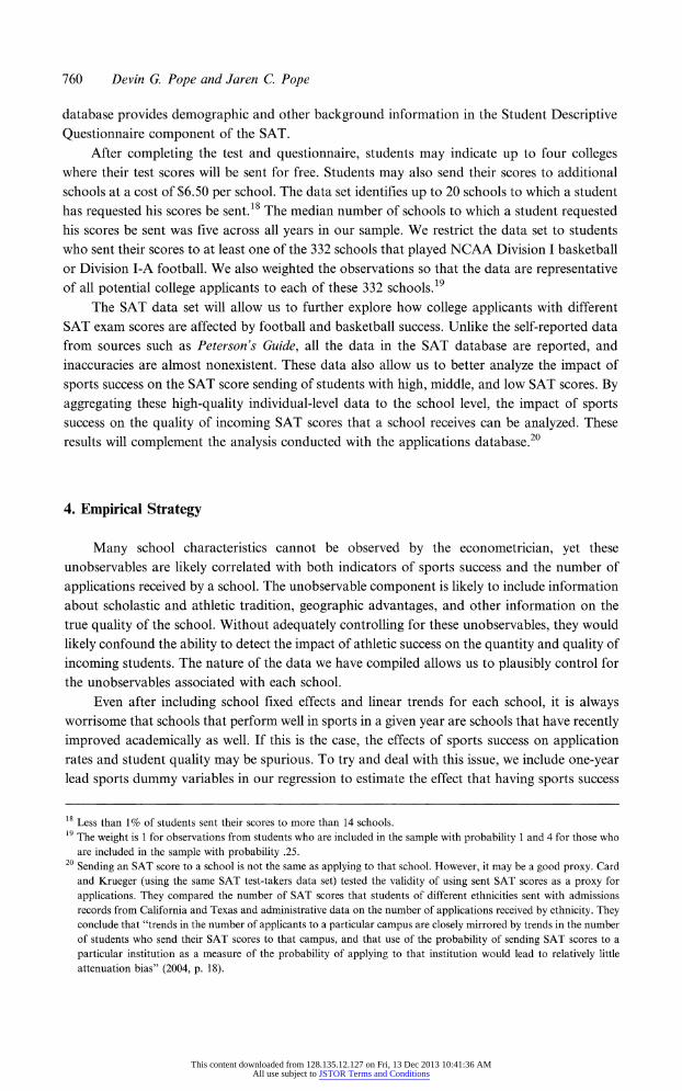
the school well before the actual deadlines. Figure 1 illustrates the distribution of application deadlines in our sample in 2003 using the Peterson's college data set. The label "continuous" in

Figure 1 refers to those schools that have a rolling application period, rather than a specific deadline. By 2003, nearly half of the schools in our sample have application deadlines in May or

earlier.

The NCAA Division I-A football season finishes at the beginning of January. The NCAA

basketball tournament finishes at the end of March or beginning of April. Therefore, if these

sports influence the number of applicants a school receives, we would expect an effect on the

current year variables. This means that a successful football team that finishes in January or a

successful basketball team that finishes in March will affect application decisions for students

enrolling that fall. However, given the timing of when applications were likely prepared and

submitted, and the football and basketball seasons, one would possibly expect an equally large

impact of football and basketball to be on the first lag of an athletic success variable (especially for basketball, which ends three months after football). The second and third lags will give an

indication of the persistence of the athletic success which occurred two to four years earlier.

5. Results

Results Using Peterson's Data

Table 3 presents the results for our specification in Equation 1 using the Peterson's college data set. The first column reports the results from a regression of log applications on the

controls and the sports variables for all schools in our sample. Standard errors in this and all




120-1

10(H

Month of Application Deadline

Figure 1. Application Deadlines

other tables presented below are computed using Eiker-White Robust standard errors. For

basketball, the results suggest that being one of the 64 teams in the NCAA tournament yields

approximately a 1% increase in applications the following year, making it to the "Sweet 16"

yields a 3% increase, the "Final Four" a 4-5% increase, and winning the tournament a 7-8%

increase. The impact of the athletic lags is as we expected. Although there is an effect of winning on the current year's applications, the largest effect comes in the first lag. By the third lag, the

effect has usually diminished substantially. Not all of the coefficients are significantly different

than zero with conventional tests. However, almost all coefficients are suggestive and several are significant. For football, the results suggest that ending the season ranked in the top 20 in

football yields approximately a 2.5% increase in applications the following year, ending in the

top 10 yields a 3% increase, and winning the football championship a 7-8% increase. The

largest effect is on the current football sports variable, along with a small effect on the first lag. Columns 2 and 3 of Table 3 report the results for log application regressions run separately for

public and private schools. The results from these regressions suggest that for basketball private schools receive two to four times as many additional applications than public schools as they advance through the NCAA tournament, while the results for football are less conclusive.

Furthermore, the application impact for private schools appears to be more persistent. For

example, when a private school advances to the Sweet 16, it enjoys an 8-14% increase in

applications for the next four years; whereas, a public school sees only a 4% increase for the next three years.

Besides being more selective, schools might react to increased applications by increasing their enrollment or tuition levels. Table 3 presents the impact of sports success on these two




variables. Column 4 uses log enrollment as the dependent variable in the now familiar

specification for all schools, and columns 5 and 6 use log enrollments of public and private schools as the dependent variable. The results indicate that teams that have basketball success

do not enroll more students the following year. However, schools that perform well on the

football field in a given year do increase enrollment that year. Teams that finish in the top 20,

top 10, and champion in football on average enroll 3.4%, 4.4%, and 10.1% more students,

respectively. These results are all significant at the 1% level. Columns 5 and 6 suggest that this is

largely driven by public schools. This increased enrollment could come from the fact that many

public schools give guaranteed admission for certain students. For example, a school that

guarantees admission for in-state students with a certain class rank or test score may be

required to enroll many more students if demand suddenly spikes. Another possible reason for

the increased enrollment is that more of the students that a university admitted decide to

actually attend that year (higher matriculation rate), which would increase enrollment.

Column 7 of Table 3 uses the log of real tuition as the dependent variable for all schools, and columns 8 and 9 use log of real tuition of public and private schools as the dependent variable. The results suggest that private schools increase tuition following trips to the Final

Four (results are also suggestive for tuition increases by private schools after winning the

basketball championship) but not for football success. There is no consistent evidence that

public schools adjust tuition because of sports success. However, this is likely because many

public schools have political constraints on increasing tuition.

Table 4 presents results using SAT data in the Petersons data set on the incoming students to see how sports success enables schools to attract higher quality students. Columns

1-3 show results from specifications that use the percent of incoming students who scored

above 500 on the SAT in math as the dependent variable for all schools, public schools, and

private schools. Columns 4-12 show results for specifications where the dependent variable is

percent of incoming students scoring above 500 in the verbal, above 600 in the math, and above

600 in the verbal section of the SAT. Overall, the coefficients in these specifications mirror to

some degree the log applications results. The results are strongest for basketball. The

coefficients on the football variables are suggestive, but not significant. The coefficients on the

basketball variables when all schools are included suggest that schools that do well in

basketball are able to recruit an incoming class with 1^% more students scoring above 500 on

the math and verbal portions of the SAT. Similarly, these schools could also expect 1-4% more

of their incoming students to score above 600 on the math and verbal portions of the SAT. As

can be seen in Table 3, however, to examine the effect of sports success on SAT score categories in the Peterson s data set, approximately 1600 observations of the 5335 are dropped due to

missing SAT data. Therefore it is important to further examine the "quality" effect using the

SAT data set.

Results Using SAT Database

The results for the impact of sports success on different SAT score subgroups are

presented in Table 5. These results stem from regressions using SAT-sending rates by SAT

subgroup and by public and private schools as the dependent variables in Equation 2. The

results indicate that sports success increases SAT-sending rates for all three SAT subgroups. However, the lower SAT scoring students (less than 900) respond to sports success about twice



Table 3. Effect of Sports Success on Applications,

Enrollment Rates, and Tuition

Log Applications Log Enrollment

Log Real Tuition All Public Private All

Public Private All Public Private

Basketball Final_64_leadl

Final_64

Final_64_lagl Final_64_lag2 Final_64_lag3 Final_16_leadl

Final_16

Final_16_lagl Final_16_lag2 Final_16_lag3

Final_4_leadl Final_4

Final_4_lagl Final_4_lag2

-0.008 -0.016*

(0.007)

(0.009)

-0.005 -0.007

(0.006)

(0.008)

0.006

0.002

(0.006)

(0.008)

0.010

0.005

(0.007)

(0.008)

0.004 -0.010

(0.007)

(0.009)

0.015

0.011

(0.010)

(0.012)

0.027***

0.023*

(0.010)

(0.012) 0.032*** 0.019

(0.010)

(0.013)

0.032***

0.024* (0.010) (0.013)

0.015

0.007

(0.011)

(0.013)

0.029

0.018

(0.019)

(0.023) 0.037** 0.023

(0.018)

(0.020)

0.044**

0.028

(0.017)

(0.019)

0.041**

0.042**

(0.017)

(0.019)

0.006 -0.008 -0.006 -0.010

(0.012)

(0.006)

(0.007) (0.009) -0.003

-0.001 0.004 -0.010 (0.011)

(0.005)

(0.007) (0.008)

0.013 -0.004 -0.002 -0.007

(0.010)

(0.006)

(0.008) (0.009) 0.019*

-0.003 -0.002 -0.007

(0.010)

(0.006)

(0.008) (0.008)

0.029***

0.001

0.000 0.004

(0.011)

(0.006)

(0.008) (0.009)

0.015 0.007 0.013 -0.004

(0.021)

(0.009)

(0.011) (0.014) 0.043**

0.015*

0.018 0.013 (0.017)

(0.009)

(0.011) (0.012) 0.062***

0.011

0.016 0.008 (0.017)

(0.009)

(0.011) (0.014) 0.049***

0.011

0.015 -0.004 (0.017)

(0.010)

(0.013) (0.016) 0.017

0.007

0.005 0.004 (0.019)

(0.009)

(0.012) (0.013)

0.032 0.011 0.017 -0.013

(0.029)

(0.020)

(0.024) (0.024)

0.081**

-0.001

0.001 -0.008 (0.035)

(0.019)

(0.023) (0.020) 0.138***

0.000

0.011 -0.008

(0.037)

(0.018)

(0.022) (0.024)

0.090***

0.003

0.009 -0.008

(0.030)

(0.019)

(0.024) (0.028)

0.016*

0.011

0.019 (0.008)

(0.009)

(0.018) 0.005

0.004

0.012 (0.007)

(0.008)

(0.012) -0.001

-0.006

0.010 (0.007)

(0.008)

(0.011) 0.002

-0.005

0.012 (0.006)

(0.008)

(0.009) -0.000

-0.009

0.015 (0.007)

(0.009)

(0.010) 0.025**

0.025**

0.013 (0.010)

(0.012)

(0.010) 0.027***

0.028**

0.011* (0.009)

(0.011)

(0.007) 0.018*

0.014

0.006 (0.009)

(0.012)

(0.008) 0.015

0.009

0.010 (0.009)

(0.012)

(0.007) 0.015

0.020

0.012* (0.010)

(0.012)

(0.007) 0.027

0.028

0.002 (0.019)

(0.020)

(0.022) 0.040** 0.025 0.063* (0.019)

(0.022)

(0.037) 0.027

0.012

0.041** (0.019)

(0.021)

(0.019) 0.003

-0.012

0.048** (0.015)

(0.017)

(0.021)

9 Hi CS CO 5^ ^3



Table 3. Continued

Log Applications

Log Enrollment

Log Real Tuition

All

Public

Private

All

Public

Private

All

Public

Private

Final_4_lag3 Champ_leadl

Champ

Champjagl Champ_lag2 Champ_lag3

Football

Top_20_leadl

Top_20

Top_20_lagl Top_20_lag2 Top_10_leadl

Top_10

Top_10_lagl Top_10_lag2

0.027 (0.020)

-0.004 (0.031)

0.039 (0.030) 0.074*** (0.017) 0.077*** (0.025)

0.051**

(0.022) 0.008

(0.010) 0.025** (0.011) 0.013

(0.011) 0.001

(0.010) 0.002

(0.013) 0.032** (0.013) 0.019

(0.013)

-0.006 (0.013)

0.022 (0.025)

0.004 (0.037)

0.047 (0.039) 0.063*** (0.023)

0.045 (0.028)

0.016 (0.023)

0.011 (0.011) 0.032*** (0.011)

0.015 (0.011)

-0.006

(0.011)

0.009 (0.014) 0.033** (0.013) 0.029** (0.014)

-0.003 (0.013)

0.079***

(0.030) -0.106**

(0.044) 0.020

(0.042) 0.092** (0.037)

0.149***

(0.032)

0.129***

(0.030) -0.034 (0.039)

-0.052 (0.045)

-0.014 (0.045)

0.026 (0.034)

-0.022 (0.031)

0.047 (0.038)

-0.006 (0.038)

-0.004 (0.038)

0.016 (0.020)

0.034 (0.030)

0.009

(0.023)

0.023 (0.027)

0.036

(0.025)

0.056* (0.032) 0.013

(0.009) 0.032*** (0.009) 0.011

(0.010) -0.005

(0.009) 0.027** (0.013) 0.044*** (0.012) -0.009 (0.011)

-0.009 (0.011)

0.031

(0.025)

0.042 (0.035)

-0.003 (0.029)

0.017 (0.035)

0.047

(0.030) 0.051

(0.041) 0.022** (0.010)

0.035***

(0.010) 0.015

(0.010) -0.007 (0.010)

0.030** (0.015)

0.038*** (0.012) -0.010 (0.013)

-0.008 (0.012)

-0.007 (0.021)

0.005 (0.050)

0.031 (0.034)

0.033 (0.032)

0.001 (0.040)

0.053 (0.044)

-0.047*** (0.018)

0.012 (0.031)

-0.032 (0.026)

0.003 (0.025)

0.035 (0.024) 0.091* (0.048)

-0.008 (0.028)

-0.017 (0.021)

-0.012

(0.021)

-0.004 (0.021)

0.008 (0.027)

0.019

(0.018)

0.003 (0.020)

0.010

(0.017)

0.001 (0.009)

0.008 (0.010)

-0.000

(0.009) 0.000

(0.010) -0.026**

(0.011)

-0.015

(0.011) -0.013 (0.010)

-0.001 (0.010)

-0.028 (0.026)

0.012 (0.028)

0.030 (0.038)

0.014 (0.025)

-0.003 (0.030)

0.017 (0.023)

0.006 (0.011)

0.011 (0.011)

0.003 (0.010)

0.001 (0.010)

-0.016 (0.011)

-0.013 (0.012)

-0.008 (0.011)

0.000 (0.012)

0.038** (0.015) -0.024 (0.027) -0.022 (0.026)

0.012

(0.025)

0.038

(0.024)

0.012 (0.024)

-0.015

(0.010) 0.001

(0.012) -0.006 (0.011)

0.014 (0.014)

-0.010 (0.018)

-0.001

(0.015) -0.006

(0.011) 0.011

(0.012)

a a a



Table 3. Continued

Log Applications Log Enrollment

Log Real Tuition All Public Private All Public Private All Public Private

Champjeadl -0.007 -0.008

0.208***

0.005 0.017 -0.049 0.015 0.017 ?

(0.033) (0.035) (0.061) (0.029) (0.032) (0.048) (0.029) (0.031) ?

Champ 0.076** 0.065* 0.227***

0.101***

0.111*** -0.002 -0.009 -0.000 ?

(0.032) (0.035) (0.066) (0.028) (0.030) (0.049) (0.023) (0.022) ?

ChampJagl -0.011 -0.014 0.119**

0.003

0.013 -0.122** -0.071 -0.023 ?

(0.047) (0.049) (0.059) (0.028) (0.030) (0.053) (0.054) (0.023) ?

Champ_lag2 -0.038 -0.042 0.063 -0.020 -0.018 0.029 0.008 -0.001 ?

(0.031) (0.034) (0.060) (0.025) (0.025) (0.054) (0.020) (0.021) ?

Year fixed effects

XXXXX X XXX School fixed

effects XXXXX X XXX

Linear trends XXXXX X XXX

Controls XXXXX X XXX

N 5335 3428 1907 5272 3398 1874 4649 3048 1601

I?_0.969 0.96_097_0.971

0.958_0.964_0.983

0.927 0.949

The table uses Peterson's data for all 332 schools that participate in Division I basketball or football.

All regressions include year and school fixed effects, school-specific linear trends,

and controls for average nine-month full-time professor salary, total annual cost of

attendance,

number of high school diplomas given out by the school's state, and per capita income in the

school's state. Robust

standard

errors are shown in parentheses.

* significant at the 10% level. **

significant at the 5% level. ***

significant at the 1% level.

Co



768 Devin G Pope and Jaren C. Pope

as much as the higher SAT scoring students. For example, schools that win the NCAA basketball tournament see an 18% increase a year later in sent SAT scores less than 900, a 12% increase in scores between 900 and 1100, and an 8% increase in scores over 1100. Also, private schools tend to see a larger increase in sent SAT scores after sports success than for public schools (although this does not appear to be true for the basketball championship and high SAT scores). For example, it can be seen that when a private school reaches the Sweet 16 in the NCAA basketball tournament, they have two to three times as many SAT scores sent to them as the pubic schools in the first and second periods after the basketball success. Furthermore, the effect tends to persist longer for the private schools than the public schools, as can be seen on lags 2 and 3. A similar difference between public and private schools can be seen for

football. The championship round cannot be compared, as there were no private schools that won the football championship during this time period.

Overall, these results suggest that schools that have athletic success are not receiving extra

SAT scores solely from low performing students. The results also greatly strengthen the SAT results derived from the Petersons data. It appears that athletic success does indeed present an

opportunity to schools to be either more selective in their admission standards or enroll more

students while keeping a fixed level of student quality.

Specification and Robustness Checks

Although the specification described in Section 4 and used to produce the results presented in Section 5 is our a priori preferred specification given our data, there are other potential specifications that could be used to analyze the impact of sports success on the quantity and

quality of student applications.22 For example, because of the panel nature of our data, one

could use the random effects model rather than the fixed effects model. Therefore we also ran a

random effects model and compared it with the fixed effects model using a Hausman test. The Hausman test rejected the null hypothesis that the coefficients estimated by the random effects estimator were the same as the ones estimated by the fixed effects estimator (Prob > %2

=

0.0000). Thus the fixed effects model appears to be appropriate for our analysis. Nevertheless, it is comforting that when comparing the random effects coefficients in column 2 of Table 6 with the fixed effects estimates in column 1, the coefficients are similar in magnitude and

significance.

Another specification assumption we made was using the log-linear functional form for our regressions. Remember that we chose this functional form because it should help mitigate the problem of overweighting large schools relative to small schools. This assumption makes sense if applications tend to increase by a given percentage across schools rather than by a given level due to sports success. However, despite this a priori intuition, we reestimated our primary

model using all schools, but this time using the total applications as our dependent variable that were not scaled. As can be seen in column 3 of Table 6, the results closely mirror our log applications results. For example, the increase of 420 applications we see for the Final_4_lagl variable is approximately a 6% increase in applications for the average school in our sample; whereas, our original specification suggests a 5.5% increase. We also run a regression where the

We are again grateful to the referees of this paper for bringing to our attention the need for some of these robustness checks.



Table 4. Effect of Sports Success on SAT Scores by Public and Private Colleges

% Math SAT > 500 % Verbal SAT > 500 % Math SAT > 600 % Verbal SAT > 600

All Public Private All Public Private All Public Private All Public Private

Basketball

Final_64_leadl -0.096 -0.349 0.242 -0.244 -0.842*

0.555 -0.373 -0.360 -0.445 -0.445 -0.845*** 0.077

(0.270) (0.372) (0.399) (0.386) (0.486)

(0.623)

(0.238) (0.300) (0.401) (0.297) (0.323) (0.539)

Final_64 -0.138 -0.480 0.465 0.336 -0.012 1.160* -0.078 -0.111 0.142 -0.038 -0.169 0.254

(0.262) (0.359) (0.389) (0.361) (0.439)

(0.599)

(0.250) (0.344) (0.384) (0.285) (0.322) (0.503)

Final_64_lagl 0.220 0.011 0.569 0.659 0.618 0.605 0.230 0.213 0.372 0.182 0.160 0.196

(0.281) (0.407) (0.396) (0.435) (0.627)

(0.590)

(0.230) (0.316) (0.363) (0.316) (0.440) (0.447)

Final_64_lag2 0.833*** 0.583 1.199*** n.662*

0.037

1.552** 0.613*** 0.726** 0.535 -0.008 -0.161 0.267

(0.276) (0.370) (0.423) (0.367) (0.425)

(0.612)

(0.237) (0.310) (0.379) (0.282) (0.300) (0.506)

Final_64_lag3 0.298 -0.290 1.052** 0.906**

0.625

1.455** 0.110 0.091 0.303 -0.397 -0.394 -0.274

(0.292) (0.365) (0.479) (0.387) (0.464)

(0.630)

(0.248) (0.291) (0.427) (0.307) (0.323) (0.552)

Final_16Jeadl 0.499 0.454 0.425 0.520

-0.272

2.050* 0.304 0.325 0.065 -0.030 -0.342 0.301

(0.451) (0.579) (0.778) (0.641) (0.761)

(1.166)

(0.436) (0.486) (0.938) (0.528) (0.642) (0.932)

Final_16 0.056 0.157 -0.199 0.923 1.444* 0.061

0.476 0.494 0.635 1.159** 1.474** 0.312

(0.462) (0.567) (0.828) (0.657) (0.752)

(1.212)

(0.415) (0.452) (0.854) (0.561) (0.606) (1.084)

Final_16_lagl 0.474 1.076* -0.606 0.732

1.877**

-0.813

1.124** 1.341*** 1.060 1.170** 1.536** 0.757

(0.469) (0.625) (0.711) (0.686) (0.752)

(1.363)

(0.471) (0.516) (0.939) (0.553) (0.614) (1.111)

Final_16_lag2 0.526 1.170**-0.628 0.234

0.719

-0.664 0.774 1.354** 0.041 0.837 0.794 1.032

(0.435) (0.537) (0.751) (0.650) (0.801)

(1.129)

(0.476) (0.621) (0.803) (0.585) (0.636) (1.216)

Final_16_lag3 -0.274 0.016 -1.432 -0.200

0.472

-1.841 -0.332 0.195 -1.719* 0.278 0.261 -0.432

(0.488) (0.569) (0.893) (0.635) (0.675)

(1.255)

(0.437) (0.460) (0.912) (0.466) (0.554) (0.908)

Final_4_leadl 0.840 1.017 1.614 0.109

0.982

-0.805 0.582 1.116 -1.516 0.318 0.363 0.021

(0.708) (0.791) (1.596) (1.106) (1.090) (2.463) (0.698) (0.750) (1.346) (0.966) (0.945) (2.079)

Final-4 1.517** 1.478** 1.930 0.872 1.147 0.769 0.992* 0.910 0.751 1.380* 0.857 2.435*

(0.744) (0.703) (1.635) (0.925) (0.951)

(1.875)

(0.594) (0.731) (0.929) (0.793) (0.864) (1.420)

Final_4_lagl 1.528** 0.833 3.153** 1.667 1.957* 0.878

1.223* 0.358 2.876*** 2.917*** 2.022* 4.920**

(0.760) (0.794) (1.500) (1.070) (1.168)

(2.246)

(0.685) (0.859) (1.076) (0.926) (1.081) (1.973)

Final_4_lag2 2.172*** 1.439* 3.707*** 0.872 1.156 -0.944

2.030*** 1.501* 3.446*** 2.229** 1.472 3.145*

(0.660) (0.807) (1.374) (1.058) (1.176)

(2.414)

(0.672) (0.889) (1.149) (0.996) (1.309) (1.791)

9 Hi ^3 On



Table 4. Continued

% Math SAT > 500

% Verbal SAT > 500

Math SAT > 600

% Verbal SAT > 600

All

Public

Private

All

Public

Private

All

Public

Private

All

Public

Private


Champ

Champ_lagl Champ_lag2 Champ_lag3

Football

Top_20_leadl

Top_20


Top_10


0.427 (0.683)

0.370 (0.960) -0.664

(1.071) 1.160

(0.901) 0.944

(0.909) -0.650

(1.030) 0.099 [0.446] 0.379 [0.491] 0.317 [0.443]

0.547

[0.474] -0.879

[0.590] 0.054 [0.506] -0.251

[0.649] 0.074 [0.537]

-0.644 (0.834)

0.354 (1.157)

-0.286 (1.277)

1.891 (1.334)

1.476 (1.316)

-1.900 (1.451)

-0.135

(0.483) 0.428

(0.507) 0.229

(0.488)

0.485

(0.505)

-1.055

(0.643) -0.076 (0.554)

-0.276 (0.707)

0.218 (0.600)

2.483** (1.133) 0.403

(1.703) -1.391

(1.606)

0.191

(1.268)

0.224 (1.321)

1.738 (1.247)

0.553 (1.266)

-1.088

(2.059) 0.822

(1.442) 0.487 (1.430) 1.256 (1.698) 1.778

(1.337) 0.798

(1.848) -1.016 (1.521)

-0.581 (1.233)

1.347

(1.364)

1.295 (2.063) 4.148***

(1.242) 3.399*

(1.801)

1.279 (1.253)

-0.226 (0.687)

-0.080

(0.761)

0.629 (0.671) 0.879

(0.770) -0.185

(0.812)

0.304

(0.818)

0.682

(0.887) 0.429

(0.769)

-0.470 (1.791) 0.909

(1.607)

0.169

(3.165) 4 055***

(1.507) 1.539

(2.546) -0.611 (1.321) -0.012

(0.669) 0.246

(0.717)

0.661 (0.693)

1.091 (0.789)

-0.359 (0.857)

0.159

(0.829) 0.369

(0.898) 1.091

(0.807)

-1.785 (1.625) 3.370

(2.632)

4.130* (2.401)

5.078*** (1.814) 3.576**

(1.819) 4.049**

(2.015) -3.644 (2.359)

-5.107 (3.565)

-0.056 (2.467)

-2.055 (2.179)

3.459 (2.386)

2.781 (2.772)

3.708 (3.494)

-3.942* (2.140)

1.469*"

(0.649) 0.341

(0.815) -1.892

(1.373)

2.000* (1.064)

1.454

(1.096) -0.067 (1.171) 0.131

(0.477)

-0.245 (0.535) -0.234 (0.452)

0.009

(0.496)

-1.221* (0.625) -0.441 (0.549) -0.254 (0.639) -0.192 (0.602)

1.054

(0.764) 0.103

(0.806)

-0.687 (1.450) 1.797

(1.162)

1.883*

(1.144) -0.131

(1.565) 0.275

(0.501) 0.076

(0.546) -0.200

(0.485) 0.199

(0.523) -1.127 (0.701) -0.351

(0.605)

-0.061 (0.700)

0.247 (0.626)

1.587 (1.020)

-0.487 (2.102)

-4.275** (1.949) 3.818** (1.584)

0.699 (1.668)

0.085

(1.553) -1.770

(1.583) -4.500**

(2.202) -0.863

(1.691) -3.105*

(1.782) 0.008

(1.556) -1.314

(1.351) -0.292

(1.935) -2.708 (2.044)

0.954 (1.104)

-2.145 (1.346)

-3.014 (2.423)

1.502 (1.791)

2.846 (2.029)

0.826

(1.631)

0.595 (0.609)

0.591

(0.605)

0.952 (0.610)

0.880 (0.565)

0.515

(0.631) 0.924

(0.619) 0.989* (0.592) 0.502

(0.662)

0.704 (1.530)

-2.380 (1.833) -4.592

(3.825)

1.625

(2.589)

4.174* (2.506)

1.430 (1.962)

1.086* (0.598)

1.085* (0.610)

0.929 (0.592)

1.054* (0.588)

0.222

(0.647)

0.894 (0.677)

0.989 (0.656)

1.189* (0.665)

1.571 (1.433) -2.804 (2.487)

-1.342

(2.033) 2.580

(2.520)

1.294

(2.762) 1.862

(3.004) -4.411**

(2.019) -7.536**'

(2.208)

-1.336

(3.388)

-2.579 (1.756) 5.478**

(2.402) 3.331

(2.103) 4.829**

(2.170) -2.148 (3.026)

^1 o b Hi S'



Table 4. Continued

% Math SAT > 500 % Verbal SAT > 500 % Math SAT > 600 % Verbal SAT > 600

All Public Private All Public Private All Public Private All Public Private

Champ Jeadl 1.359 1.636 0.778 1.791 2.004 6.200

3.460* 4.038* 3.762 1.465 1.493 9.001

[1.221] (1.273) (2.738) (1.758) (1.948) (4.557) (1.961) (2.161) (3.176) (1.770) (2.160) (3.540)

Champ 2.47 2.510 -2.000 1.490 1.597

-2.834

1.984 1.985 0.489 1.300 1.058 -0.038

[1.692] (1.852) (2.280) (2.052) (2.249)

(3.785)

(2.136) (2.410) (2.899) (1.781) (2.076) (4.397)

Champ Jagl 0.934 0.627 -1.087 1.616

0.782

0.428 0.708 0.422 4.534 2.458 2.047 0.774

[1.081] (1.257) (2.436) (2.061) (2.237) (4.166) (1.708) (1.933) (2.980) (1.654) (1.923) (3.505)

Champ_lag2 0.926 0.864 -3.096 1.268 1.276 0.095 1.366 1.405 2.717 0.077 0.093 0.716

[1.124] (1.240) (2.281) (1.767) (1.885) (4.037) (1.549) (1.710) (2.930) (1.686) (1.931) (3.268)

Year fixed effects XXXXXXXXXXXX School fixed

effects XXXXXXXXXXXX

Linear

trends

XXXXXXXXXXXX

Controls XXXXXXXXXXXX

N 3725 2068 1657 3724 2068 1656 3711 2059 1652 3697 2046 1651

r2 0.963 0.965 0.957 0.948 0.947

0.944

0.977 0.970 0.979 0.960 0.944 0.964

The table uses Peterson's data for all 332 schools that participate in Division I basketball or football. All regressions include year and school fixed effects, school-specific linear trends,

and controls for average nine-month full-time professor salary, total annual cost of

attendance,

number of high school diplomas given out by the school's state, and per capita income in the

school's state. Robust standard errors are shown in parentheses.

*

significant

at the 10% level. ** significant at the 5% level. *** significant at the 1% level.

f fib Co a*1 ^1




dependent variable is the total applications in a given year divided by the number of these

applications that actually enrolled in the school. This specification, like the log of applications, scales applications to help account for the size of the school. Column 4 presents the results of

this regression and shows that for basketball the results are similar to our original results

(although somewhat larger in magnitude); whereas, the football results are less significant (and smaller in magnitude). We think this reflects an issue of endogeneity, since we showed in

Table 3 that enrollments do increase after sports success, especially for football schools. Thus, as applications increase, so do enrollments, so that the impact in our dependent variable is

naturally dampened. Overall, these regressions do not suggest that using the log of applications was inappropriate.

Another potential concern is that our school fixed effects and linear trends do not fully

capture changes in the quality of schools over time and therefore may confound the analysis.

Although the original specification includes four additional school quality variables, it may be

useful to include additional variables in the Xi>t portion of the specification to better control for

changes in school quality over time. The reason for not including these variables in the original

specification is because they are typically not available for all of the schools or all of the time

period of our analysis. Therefore, using additional control variables comes at the cost of

statistical power. Nonetheless, we did acquire the following additional school quality variables

for schools over time that have appeared in higher education literature: publication and citation

data, federal grant dollars acquired, percentage of students that go on to graduate school,

faculty to student ratio, percentage of student body that are graduate students, per capita

expenditure on instruction, number of national merit achievement scholars, percentage of

faculty with a doctorate, and the number of volumes in the school library.23 We include these variables in Xi>t as a robustness test. Column 5 of Table 6 presents the

results from this regression. Although using these additional controls causes us to lose

approximately 25% of our sample, these results also closely mirror our original specification. A final unreported specification check that was suggested by a referee was to add some geographic variables in case changes in application rates are somehow spatially correlated within regions. A specification that added census regions found virtually no

change in the coefficients on our sports success variables. Therefore, as a whole these

specification and robustness checks suggest that our original specification is a reasonably robust one for the task of identifying the impact of sports success on the quantity and quality of

student applications.

6. Conclusion and Future Research

"How does playing major college football or men's basketball in a highly commercialized,

profit-seeking, entertainment environment further the educational purpose of your member

institutions?" Fully answering Representative Thomas's question that he posed to the president

Publication and citation data came from Thomson's University Science Indicators database, federal grant dollars and

per capita expenditure on instruction were derived from IPEDS, and all other additional variables were derived from

the Petersons data we purchased. It should be noted that in an effort to reduce the number of observations that were

dropped, some of the observations were interpolated or extrapolated from observations on a school level where data were not collected every year.



Table 5. Effect of Sports Success

on Number of SAT Scores Sent by SAT Group

Log SAT Scores Where SAT < 900

Log SAT Scores Where 900 < SAT < 1100

Log SAT Scores Where SAT > 1100

All

Public

Private

All

Public

Private

All

Public

Private

Basketball

Final_64_leadl

Final_64


Final_16


Final_4


0.014 (0.009) 0.021** (0.009)

0.045***

(0.010) 0.033*** (0.010) 0.007

(0.009) -0.017 (0.016) 0.028* (0.016) 0.076*** (0.017) 0.051*** (0.015) 0.025* (0.015) 0.036* (0.021) 0.051** (0.022) 0.116*** (0.021) 0.088*** (0.020)

0.012 (0.010) 0.028** (0.012) 0.043*** (0.012) 0.022* (0.011)

-0.008 (0.011)

-0.012

(0.015) 0.015

(0.018) 0.039** (0.018) 0.030**

(0.015)

-0.001 (0.014) 0.053** (0.024) 0.080*** (0.024) 0.112*** (0.024) 0.084*** (0.024)

0.007 (0.016)

0.007 (0.016) 0.039** (0.018)

0.046**

(0.018) 0.031* (0.016) -0.031

(0.047)

0.070* (0.038)

0.158***

(0.035) 0.098***

(0.037)

0.084** (0.038) 0.022

(0.050) -0.011 (0.058) 0.122** (0.057) 0.153***

(0.050)

0.007

(0.008) 0.009

(0.008) 0.030*** (0.009) 0.022** (0.010) 0.011

(0.009) -0.002 (0.016)

0.017 (0.013) 0.052*** (0.013) 0.054*** (0.013)

0.027**

(0.012) 0.013

(0.016) 0.014

(0.021) 0.059*** (0.018) 0.016

(0.018)

0.011 (0.011)

0.014 (0.010)

0.025**

(0.011) 0.013

(0.013) -0.002

(0.010) 0.015

(0.014) 0.012

(0.014) 0.045*** (0.014) 0.025*

(0.013)

0.016

(0.013)

0.022 (0.019)

0.015 (0.024) 0.066*** (0.021)

0.010 (0.020)

-0.005 (0.015)

-0.007 (0.014) 0.031* (0.016) 0.033**

(0.015)

0.034**

(0.015)

-0.037 (0.051) 0.038

(0.031)

0.067**

(0.029) 0.126*** (0.031) 0.048* (0.027) 0.012

(0.047) 0.050

(0.071) 0.061

(0.054) 0.086* (0.049)

-0.013 (0.010)

-0.003 (0.010)

0.012 (0.011) -0.001 (0.010) -0.021 (0.013)

-0.005

(0.012) 0.001

(0.013) 0.035*** (0.013) 0.029** (0.012)

-0.005

(0.014) -0.014

(0.018) 0.026

(0.021) 0.044** (0.020) 0.020

(0.022)

-0.016 (0.014)

0.005

(0.015) 0.011

(0.015) -0.004

(0.013) -0.030

(0.020) 0.000

(0.014) 0.005

(0.017) 0.029* (0.016) 0.019

(0.014) -0.005

(0.017) -0.006

(0.021) 0.050** (0.021)

0.052**

(0.023) 0.024

(0.027)

-0.014 (0.014)

-0.017

(0.014)

0.017 (0.017)

0.002 (0.014)

-0.004 (0.014)

-0.014

(0.027)

-0.006

(0.025) 0.049*

(0.026) 0.058** (0.026) -0.005 (0.023) -0.013

(0.037)

-0.011

(0.063)

-0.001 (0.042) -0.003 (0.040)

f CO a o



Table 5. Continued

Log SAT Scores Where SAT < 900

Log SAT Scores Where 900 < SAT < 1100

Log SAT Scores Where SAT > 1100

All

Public

Private

All

Public

Private

All

Public

Private


Champ

Champjagl Champ_lag2 Champ_lag3

Football


Top_10


Champ_leadl Champ

0.041* (0.021) 0.008

(0.028) 0.025

(0.026) 0.178*** (0.032) (0.029) 0.099*** (0.026) 0.032** (0.014) 0.032** (0.012)

0.007 (0.015)

0.033**

(0.015)

0.081***

(0.016) 0.040***

(0.014) -0.102*** (0.039)

0.056*

(0.032)

0.017 (0.022) -0.002 (0.037)

0.042 (0.033)

0.172***

(0.030) 0.186*** (0.032)

0.093*** (0.033) 0.026

(0.016) 0.026* (0.014) 0.006

(0.015) 0.016

(0.015) 0.059***

(0.015) 0.027*

(0.015)

-0.077** (0.038) 0.061* (0.032)

0.171***

(0.055) -0.069

(0.104) -0.176

(0.108) 0.000

(0.000) 0.205*** (0.068) 0.220*** (0.072) 0.065*** (0.024) 0.031

(0.032) -0.037 (0.043) 0.127*** (0.039)

q 179***

(0.059) 0.116*** (0.033) 0.000

(0.000) 0.000

(0.000)

0.015 (0.024)

-0.032 (0.024) -0.001 (0.021)

0.112***

(0.025) 0.092***

(0.025)

0.053** (0.025) 0.042***

(0.012)

0.039***

(0.010)

-0.000

(0.012) 0.027**

(0.011) 0.059*** (0.011) 0.031***

(0.011)

-0.013 (0.022)

0.082***

(0.024)

-0.001 (0.025) -0.011 (0.028)

0.015

(0.026) 0.131*** (0.025) 0.094*** (0.032) 0.065** (0.030) 0.038*** (0.014)

0.036***

(0.012) 0.002

(0.013) 0.026** (0.012)

0.055***

(0.011) 0.022* (0.012) -0.003 (0.023) 0.092*** (0.023)

0.154*** (0.057) -0.137

(0.122)

-0.085

(0.136)

0.000

(0.000)

0.073

(0.096) 0.061

(0.074) 0.069***

(0.024)

0.037*

(0.023) -0.063**

(0.030)

0.007 (0.033)

0.077*

(0.044) 0.095***

(0.034)

0.000

(0.000)

0.000

(0.000)

-0.006 (0.020) -0.079*** (0.027)

-0.047 (0.033) 0.085*** (0.031) 0.055* (0.030)

-0.023 (0.034) 0.027** (0.013) 0.019* (0.011)

-0.000 (0.014)

0.011 (0.012) 0.052*** (0.012) 0.023** (0.011)

-0.009 (0.028) 0.103*** (0.033)

-0.002 (0.024)

-0.063** (0.032) -0.027 (0.036) 0.109*** (0.034) 0.091*** (0.030)

0.008 (0.042) 0.026*

(0.015)

0.010 (0.012)

0.003 (0.014)

0.004 (0.014) 0.045*** (0.013)

0.012 (0.013)

0.012 (0.029) 0.109*** (0.034)

-0.020 (0.052)

-0.096

(0.093)

-0.026

(0.118) 0.000

(0.000) -0.068 (0.083) -0.007

(0.061) 0.043

(0.029) 0.050** (0.022) -0.059

(0.054) 0.039

(0.027) 0.092** (0.041) 0.058

(0.042) 0.000

(0.000) 0.000

(0.000)

^1 b I ? i



Table 5. Continued

Log SAT Scores Where SAT < 900 Log SAT

Scores Where

900 < SAT < 1100 Log SAT Scores Where SAT > 1100

All Public Private All Public Private All Public Private

Champjagl 0.119*** 0.124*** 0.000 0.112*** 0.117*** 0.000 0.126*** 0.130*** 0.000

(0.041) (0.040) (0.000) (0.024)

(0.024)

(0.000) (0.036) (0.038) (0.000)

Champ_lag2 0.028 0.029 0.000

0.025

0.018 0.000 0.000 -0.004 0.000

(0.048) (0.046) (0.000) (0.033)

(0.034)

(0.000) (0.038) (0.039) (0.000)

Year fixed effects XXXXXXXXX

School fixed effects XXXXXXXXX

Linear

trends

XXXXXXXXX

Controls XXXXXXXXX

N 2429 1563 866 2428 1562 866 2430 1564 866

R2 0.995 0.996 0.992 0.996 0.997 0.992 0.996 0.995 0.996

The table uses Peterson's data for all 332 schools that participate in Division I basketball

or football. All regressions include year and school fixed effects, school-specific linear trends,

and controls for average nine-month full-time professor salary, total annual cost of attendance, number of high school diplomas given out by the school's state, and per capita income in the

school's state. Robust

standard

errors are shown in parentheses.

* significant at the 10% level. **


significant

at the 1% level.

CO a C<3




of the NCAA is beyond the scope of this study. However, the analysis presented above

does provide a set of estimates about the impact of sports success on the quantity and quality of student applications at schools participating in the premier divisions of NCAA basketball

and football. These estimates reflect several indirect benefits from these high-profile college

sports.

Using two unique and comprehensive data sets in conjunction with an econometric design that controls for the unobservable features of schools, we find that football and basketball success increases the quantity of applications to a school after that school achieves sports success, with estimates ranging from 2% to 8% for the top 20 football schools and the top 16

basketball schools each year.24 We also provide evidence that the extra applications are

composed of students with both low and high SAT scores. Additional evidence suggests that

schools use these extra applications to increase both student quality and enrollment size. There

is some evidence that private schools adjust tuition levels in response to receiving extra

applications from basketball success.

A related paper (Pope and Pope 2007) shows that sports success has a heterogeneous

impact on various subgroups of the incoming student population. For example, we found that

males, blacks, and students that played sports in high school are more likely to be influenced by sports success than their peers. This finding, combined with the results of this paper, provides a

much broader picture of the impact of sports success on the composition of the incoming student body. These results significantly extend the existing literature and provide important

insights about the impact of sports success on college choice. Using identification strategies that

exploit the temporal variation in our data sets and that control for unobserved school

heterogeneity, it is increasingly clear that sports success does have an impact on the incoming freshman classes. It is also clear that this impact is often short lived, and that it differs by student type. This may reflect differences in the ability of various student subgroups to acquire

quality information that would affect school choice, or it may simply reflect preferences for

high-quality athletics.

Whether or not the expenditures required to receive these short-run indirect benefits

promote efficiency in higher education was not determined in the present analysis. Indeed, the raw summary data in Table 2 would suggest that athletically successful schools actually saw

slightly slower long-run growth in applications and enrollments. Future work directed at

understanding the arms-race nature of athletics within higher education and its relation to

economic efficiency would certainly be valuable. Nonetheless, the results presented in this paper should be important to college administrators. Athletics is one instrument that institutions of

higher education have at their disposal that can be used to directly affect reputation and the

prominence of their schools. It is hoped that these results provide information that can aid

administrators in making decisions about athletic programs and help them to further

understand the role of athletics within higher education.

24 To put this quantity effect into perspective, the application elasticity of changes in the price of attending college found

in the literature typically range from -.25 on the low end to -1.0 on the high end (see, e.g., Savoca 1990; Curs and

Singell 2002). These elasticities suggest that tuition/financial aid would have to be adjusted somewhere in the range of

2-24% to obtain a similar increase in applications.



Table 6. Specification

and Robustness Checks

Log Applications with

Original Controls

Log Applications Using Random Effects

Applications

Applications Scaled by Enrollments


Additional Controls

Basketball Final_64_leadl Final_64

Final_64_lagl Final_64_lag2 Final_64_lag3

Final_16_leadl

Final_16

Final_16_lagl

Final_16_lag2 Final_16_lag3

Final_4_leadl Final_4


Final_4_lag3

-0.008 (0.007)

-0.005 (0.006)

0.006 (0.006)

0.010 (0.007)

0.004 (0.007)

0.015 (0.010) 0.027*** (0.010) 0.032*** (0.010) 0.032*** (0.010)

0.015 (0.011)

0.029 (0.019) 0.037** (0.018) 0.044** (0.017) 0.041** (0.017)

0.027 (0.020)

-0.005 (0.008)

-0.002

(0.008)

0.013 (0.008) 0.017** (0.008)

0.012 (0.008)

0.005 (0.013)

0.017 (0.012) 0.025** (0.013)

0.022 (0.013)

0.007 (0.013)

0.027 (0.022) 0.041* (0.022) 0.055** (0.024) 0.051** (0.024)

0.029 (0.024)

-28.407

(57.018)

-74.437

(49.962) -48.063

(48.495) 60.406

(53.262)

6.132

(52.930) 140.705 (104.637) 182.112*

(107.101)

164.942 (111.833) 217.242**

(107.261)

117.029

(106.079)

282.445 (197.845)

399.343** (187.624)

419.682** (194.402) 317.387**

(158.052)

162.676 (184.903)

0.019 (0.027)

-0.008

(0.025)

0.049** (0.024) 0.058** (0.024) 0.011

(0.026) 0.038

(0.039) 0.050

(0.040) (0.040) 0.106** (0.043) 0.054

(0.046)

0.080 (0.061) 0.150* (0.078) 0.213** (0.088) 0.186** (0.073)

0.118 (0.082)

-0.004 (0.007)

-0.005 (0.007)

0.002 (0.006)

0.008 (0.007)

0.001 (0.007)

0.020**

(0.010) 0.023** (0.010)

0.025**

(0.011)

0.033***

(0.011) 0.019* (0.010)

0.056***

(0.020) 0.059*** (0.018)

0.064***

(0.018) 0.060*** (0.017) 0.045** (0.021)

9 'S Co ^3 -0



Table 6. Continued


Original Controls

Log Applications Using Random Effects

Applications

Applications Scaled by Enrollments


Additional Controls

Champ_leadl Champ

Champ_lagl Champ_lag2 Champ_lag3

Football

Top_20_leadl Top_20


Top_10

Top_10_lagl Top_10_lag2 Champ_leadl

-0.004 (0.031)

0.039 (0.030) 0.074*** (0.017)

0.077***

(0.025) 0.051** (0.022) 0.008

(0.010) 0.025** (0.011) 0.013

(0.011) 0.001

(0.010) 0.002

(0.013) 0.032** (0.013) 0.019

(0.013) -0.006 (0.013)

-0.007 (0.033)

0.013 (0.044)

0.060

(0.044) 0.077** (0.031) 0.083** (0.033) 0.047*

(0.027)

0.002 (0.012)

0.018 (0.013)

0.003 (0.012)

-0.008 (0.012)

-0.010

(0.016)

0.029* (0.016) 0.012

(0.017) -0.005

(0.014) -0.004

(0.038)

-319.290 (385.772)

-116.119 (315.222) 413.731*

(211.601) 373.573 (325.704) 209.856 (266.961)

24.879

(137.639)

240.797* (139.887) 97.064

(138.090)

84.961

(134.192)

-89.370

(176.871) 260.194

(176.847)

159.405

(170.504) -101.202

(174.112) -124.825

(441.554)

-0.233 (0.168)

-0.054 (0.109)

0.157 (0.126)

0.270* (0.164)

0.098 (0.124) -0.021 (0.041)

-0.015 (0.047)

0.021 (0.043)

0.030 (0.038)

-0.059 (0.052)

-0.018 (0.060) 0.103* (0.053)

0.018 (0.050)

0.000 (0.120)

-0.010 (0.034)

0.051 (0.031) 0.062*** (0.018) 0.066*** (0.025)

0.037 (0.024)

0.013 (0.011) 0.030*** (0.011) 0.019* (0.010)

0.003 (0.010)

0.012 (0.013) 0.043*** (0.013) 0.028** (0.013)

0.000 (0.013)

-0.006 (0.030)

^1 00 b Hi ?



Table 6. Continued


Original Controls

Log Applications Using

Random Effects

Applications

Applications Scaled by

Enrollments


Additional Controls

Champ

Champjagl Champ_lag2 Year fixed effects School fixed effects

School random effects

Linear trends Original controls

Add.

controls

N R2

0.076** (0.032) -0.011 (0.047)

-0.038 (0.031)

X X X X

5335 0.969

0.094** (0.039) 0.006

(0.056) -0.041

(0.037)

X X X X

5335 0.947

1,015.863* (538.129)

-135.378

(800.892) -399.336

(483.546)

X X X X

5335

0.963

0.017

(0.127) 0.014

(0.147) -0.004

(0.104)

X X X X

5197 0.920

0.079***

(0.028) 0.002 (0.040) -0.039 (0.030) X X X X X

4082 0.976

The table uses Peterson's data for all 332 schools that participate in Division I

basketball or football. All regressions include year and school fixed effects and school-specific linear

trends. Robust standard errors are shown in parentheses.

* significant

at the 10% level. **


significant

at the 1% level.

9 f <^ CO I a I 5' a




References

Avery, C, and C. Hoxby. 2004. Do and should financial aid decisions affect students' college choices? In College choices: The new economics of choosing, attending, and completing college, edited by Caroline Hoxby. Chicago: University of Chicago Press, pp. 239-299.

Bremmer, D., and R. Kesselring. 1993. The advertising effect of university athletic success?A reappraisal of the

evidence. Quarterly Review of Economics and Finance 33:409-21.

Card, D., and A. Krueger. 2004. Would the elimination of affirmative action affect highly qualified minority applicants? Evidence from California and Texas. NBER Working Paper No. 10366.

Chapman, D. 1981. A model of student college choice. Journal of Higher Education 52:490-503.

Coughlin, C, and O. Erekson. 1984. An examination of contributions to support intercollegiate athletics. Southern Economic Journal 51:180-95.

Curs, B., and L. D. Singell. 2002. An analysis of the application and enrollment process for in-state and out-of-state

students at a large public university. Economics of Education Review 21:111-24.

Fuller, W., C. Manski, and D. Wise. 1982. New evidence on the economic determinants of post secondary schooling choices. Journal of Human Resources 17:477-95.

Goidel, R., and J. Hamilton. 2006. Strengthening higher education through gridiron success? Public perceptions of the

impact of national football championships on academic quality. Social Science Quarterly 87:851-62.

McCormick, R., and M. Tinsley. 1987. Athletics versus academics? Evidence from SAT scores. Journal of Political

Economy 95:1103-16.

McEvoy, C. 2006. The impact of elite individual athletic performance on university applicants for admission in NCAA

Division I-A football. The Sport Journal 9(1).

Mixon, F. 1995. Athletics versus academics? Rejoining the evidence from SAT scores. Education Economics 3:277-83.

Mixon, F., and Y. Hsing. 1994. The determinants of out-of-state enrollments in higher education: A Tobit analysis. Economics of Education Review 13:329-35.

Mixon, F., and R. Ressler. 1995. An empirical note on the impact of college athletics on tuition revenues. Applied Economics Letters 2:383-7.

Mixon, F., and L. Trevino. 2005. From kickoff to commencement: The positive role of intercollegiate athletics in higher education. Economics of Education Review 24:97-102.

Mixon, F., L. Trevino, and T. Minto. 2004. Touchdowns and test scores: Exploring the relationship between athletics and academics. Applied Economics Letters 11:421-4.

Murphy, R., and G. Trandel. 1994. The relation between a university's football record and the size of its applicant pool. Economics of Education Review 13:265-70.

Pope, D., and J. Pope. 2007. Consideration set formation in the college choice process. Unpublished paper, The Wharton School and Virginia Tech.

Savoca, E. 1990. Another look at the demand for higher education: Measuring the price sensitivity of the decision to

apply to college. Economics of Education Review 9:123-34.

Siegfried, J., and M. Getz. 2006. Where do the children of professors attend college? Economics of Education Review

25:201-10.

Tucker, I. 2004. A reexamination of the effect of big-time football and basketball success on graduation rates and alumni

giving rates. Economics of Education Review 23:655-61.

Tucker, I. 2005. Big-time pigskin success. Journal of Sports Economics 6:222-9.

Tucker, I., and L. Amato. 1993. Does big-time success in football or basketball affect SAT scores? Economics of Education Review 12:177-81.

Tucker, I., and L. Amato. 2006. A reinvestigation of the relationship between big-time basketball success and average SAT scores. Journal of Sports Economics 7:428^40.

Zimbalist, A. 1999. Unpaid professionals: Commercialism and conflict in big-time college sports. Princeton, NJ: Princeton

University Press.



Documents

The Impact of College Sports Success on the Quantity and ...faculty.chicagobooth.edu/devin.pope/research/pdf/Website_SEJ Sports... · intercollegiate athletics is akin to an "arms