Embed Size (px)
Citation preview
American Economic Review 2013, 103(2): 585–623 http://dx.doi.org/10.1257/aer.103.2.585
585
Designing Random Allocation Mechanisms: Theory and Applications†
By Eric Budish, Yeon-Koo Che, Fuhito Kojima, and Paul Milgrom*
Randomization is commonplace in everyday resource allocation. We generalize the theory of randomized assignment to accommodate multi-unit allocations and various real-world constraints, such as group-specific quotas (“controlled choice”) in school choice and house allocation, and scheduling and curriculum constraints in course allocation. We develop new mechanisms that are ex ante effi-cient and fair in these environments, and that incorporate certain non-additive substitutable preferences. We also develop a “utility guarantee” technique that limits ex post unfairness in random allo-cations, supplementing the ex ante fairness promoted by random-ization. This can be applied to multi-unit assignment problems and certain two-sided matching problems. (JEL C78, D82)
Randomization is commonplace in everyday resource allocation. It is used to break ties among students applying for overdemanded public schools and for popular after-school programs, to ration offices, parking spaces, and tasks among employees, to allocate courses and dormitory rooms amongst college students, and to assign jury and military duties among citizens.1 Randomization is sensible in these examples and many others because the objects to be assigned are indivisible and monetary transfers are limited or unavailable.2 In these circumstances, any non-random assignment of resources is likely to be asymmetric and perceived as unfair. Randomization can restore symmetry, and thus a measure of fairness.
1 Lotteries played historical roles in assigning public lands to homesteaders (Oklahoma Land Lottery of 1901), and radio spectra to broadcasting companies (FCC assignment of radio frequencies during 1981–1993). Lotteries are also used annually to select 50,000 winners of the US permanent residency visas (“green cards”) from those qualified in the Department of Justice’s immigration diversity program.
2 The limitation of monetary transfers often arises from moral objection to “commoditizing” objects such as human organs, or from other fairness considerations (Roth 2007). Assignment of resources based on prices often favors those with the most wealth rather than those most deserving, and can be regarded as unfair for many goods and services. See Che, Gale, and Kim (forthcoming) for an argument along these lines based on utilitarian efficiency.
* Budish: University of Chicago Booth School of Business, 5807 S. Woodlawn Ave., Chicago, IL 60637 (e-mail: [email protected]); Che: Department of Economics, Columbia University, 420 West 118th Street, 1016 IAB, New York, NY 10027, and YERI, Yonsei University (e-mail: [email protected]); Kojima: Department of Economics, Stanford University, 450 Serra Mall, Stanford, CA 94305 (e-mail: [email protected]); Milgrom: Department of Economics, Stanford University, 450 Serra Mall, Stanford, CA 94305 (e-mail: [email protected]). We are grateful to Emir Kamenica, Sebastien Lahaie, Mihai Manea, Herve Moulin, Tayfun Sönmez, Al Roth, Utku Ünver, and seminar participants at Boston College, Gakushuin, Johns Hopkins, Princeton, Tokyo, UC San Diego, Waseda, Yahoo! Research, and Yale for helpful comments. We especially thank Tomomi Matsui, Akihisa Tamura, Jay Sethuraman, and Rakesh Vohra. Yeon-Koo Che is grateful to Korea Research Foundation for World Class University Grant, R32-2008-000-10056-0. Paul Milgrom’s research was supported by NSF grant SES-0648293.
† To view additional materials, visit the article page at http://dx.doi.org/10.1257/aer.103.2.585.
586 THE AMERICAN ECONOMIC REVIEW ApRIl 2013
In practice, the most common way to incorporate randomness into an allocation mechanism is to randomly prioritize the agents, and then use a deterministic mecha-nism. The canonical example of this approach is the popular method known as the “random serial dictatorship” (RSD), which randomly orders the agents, and then lets them choose objects one at a time in order.3 Other examples of this approach include the variants of Gale and Shapley’s deferred acceptance algorithm (Gale and Shapley 1962) and Gale’s top trading cycles algorithm (Shapley and Scarf 1974) that have been proposed for use in school choice settings. Random priorities are used to break ties in schools’ preferences (priorities) for students, after which deferred acceptance or top trading cycles can be run in the standard manner.4 These random mechanisms inherit many of the attractive properties of their deterministic counterparts; in par-ticular, they often lead to allocations that are Pareto efficient ex post. However, it is now well known that this method of randomization can introduce inefficiencies ex ante (Bogomolnaia and Moulin 2001). That is, there may exist other random allocations that give every agent in the economy greater expected utility.5
Hylland and Zeckhauser (1979)—henceforth, HZ—and Bogomolnaia and Moulin (2001)—henceforth, BM—propose mechanisms that find ex ante efficient alloca-tions, by developing an alternative approach to the random allocation of indivis-ible objects. Instead of using random priorities to select a deterministic mechanism, the HZ and BM approach focuses directly on the lotteries agents should receive. Specifically, their mechanisms directly identify an expected assignment matrix X = [ x ia ], where entry x ia describes the probability with which agent i gets object a. Focusing directly on the lotteries agents receive is convenient for finding random allocations that have desirable ex ante welfare properties. For instance, HZ’s pseudo-market mechanism finds the random allocation that would emerge were there com-petitive markets for probability shares; agents are endowed with equal budgets of an artificial currency, which they use to “buy” their most preferred affordable bundle at market clearing prices. This allocation is ex ante efficient by the first welfare theo-rem. Similarly, BM’s probabilistic serial mechanism finds an outcome that is ex ante efficient in an ordinal sense, by imagining that agents “eat” probability shares of their most preferred remaining objects, continuously over a unit time interval.
While ingenious, the HZ and BM approach has to date been limited in an impor-tant way, confining attention to the setting in which n indivisible objects are to be assigned among n agents, one for each. This limits the practical usefulness of this theoretically appealing methodology.6 The purpose of the present paper is to expand the HZ and BM approach to a much richer class of matching and assign-ment environments. Our analysis yields generalizations of HZ’s and BM’s specific mechanisms, and also yields methodological tools that may prove useful for other
3 That is, RSD uniform randomly draws a “serial order” of the agents, and then runs the corresponding (deter-ministic) serial dictatorship (Abdulkadiro ̆ g lu and Sönmez 1998). RSD is widely used for many of the allocation problems listed above. See Chen and Sönmez (2002), Baccara et al. (2012), and Budish and Cantillon (2012) for empirical studies of variants on RSD.
4 See Abdulkadiro ̆ g lu and Sönmez (2003b) and Abdulkadiro ̆ g lu, Pathak, and Roth (2009). In fact, these random variants of Gale and Shapley’s deferred acceptance algorithm and Gale’s top trading cycles algorithm are in certain settings equivalent to RSD; see Abdulkadiro ̆ g lu and Sönmez (1998) and Pathak and Sethuraman (2011).
5 For an illustration see the example at the beginning of Section II.6 Indeed, but for the estate division application described by Pratt and Zeckhauser (1990) we are not aware of
either mechanism ever being used in practice. See footnotes 21 and 34 for more details on the set of environments for which HZ’s and BM’s original mechanisms are suited.
587budish et al.: designing random allocation mechanismsVol. 103 no. 2
designers. Our model is richer in several important ways. First of all, our model encompasses problems with multi-unit supply (e.g., schools have multiple slots), multi-unit demand (e.g., students take multiple courses), and with the possibility that agents or objects remain unassigned (e.g., a school may have excess capacity). Second, our extension accommodates a wide variety of constraints that are encoun-tered in real-world settings. A case in point is “controlled choice” constraints in school assignment, whereby schools are constrained to balance their student bodies in terms of gender, ethnicity, income, test scores, or geography. For instance, public schools in Massachusetts are discouraged by the Racial Imbalance Law from hav-ing student enrollments that are more than 50 percent minority.7 Another example is the scheduling constraints that arise in the context of course allocation: students are typically prohibited from enrolling in multiple courses that meet during the same time slot. Also, there may be curricular constraints that require a student to take at least a certain number of courses in some discipline, or at most a certain number.
The first part of our paper tackles a methodological issue that is raised by our richer class of problems. An expected assignment describes the “marginal” prob-abilities with which each agent receives each object. In order to actually implement an expected assignment, one must find a lottery over pure assignments—a “joint distribution”— that resolves the randomness in a way that respects the underlying constraints. HZ and BM are able to resolve this issue by appeal to a result known as the Birkhoff-von Neumann theorem.8 We provide a maximal generalization of Birkhoff-von Neumann, enabling implementation of expected assignments in a broader class of environments. First, using well-known results in the combinato-rial optimization literature, we identify a condition on the set of constraints of the allocation problem that is sufficient to guarantee that any expected assignment that satisfies the constraints in expectation can in fact be implemented. Then we dem-onstrate that the same condition is not only sufficient, but also necessary in two-sided assignment and matching environments. Together, these two results identify the maximum scope for the methodology pioneered by HZ and BM.
The rest of our paper explores applications. Our first application is a generaliza-tion of BM’s probabilistic serial mechanism, intended for applications like school choice in which there are multiple slots in each school and various constraints gov-erning how these slots are assigned. One example is the controlled choice constraints described above. Another kind of constraint occurs when a school district installs multiple school programs in a single building, and wishes to allow the enrollments in each specific program to respond to demand, subject to the total capacity of the
7 There are many other variations of controlled choice constraints. One example is Miami-Dade County Public Schools, which control for the socioeconomic status of students in order to diminish concentrations of low-income students at certain schools. In New York City, “Educational Option” (EdOpt) schools must balance their student bodies in terms of students’ test scores. In particular, 16 percent of students that attend an EdOpt school must score above grade level on the standardized English Language Arts test, 68 percent must score at grade level, and the remaining 16 percent must score below grade level (Abdulkadiro ̆ g lu, Pathak, and Roth 2005). In Seoul, public schools restrict the number of seats for those students residing in distant school districts, in order to alleviate morn-ing commutes.
8 The Birkhoff-von Neumann theorem states that any expected assignment matrix in which rows sum to one and columns sum to one can be expressed as a convex combination of pure assignment matrices, in which rows and columns still sum to one but now all entries are zero or one. Thus, in the n agent-n object setting of HZ and BM, any expected assignment that is consistent with the unit demand and supply constraints in expectation can in fact be implemented.
588 THE AMERICAN ECONOMIC REVIEW ApRIl 2013
building. As in the original BM algorithm, agents continuously “eat” their most pre-ferred available object over a unit time interval; however, the meaning of “available” has to be modified to account for the constraints. Our sufficiency result implies that the expected assignment that results from this generalization of BM’s algorithm is implementable. We then prove that the attractive efficiency and fairness properties of BM’s algorithm in its original setting extend to this more general environment.
Our second application is a generalization of HZ’s pseudo-market mechanism to the case of many-to-many matching. Examples include the assignment of course schedules to students, and the assignment of shifts to interchangeable workers. As in HZ’s original mechanism, agents are endowed with equal budgets of an artificial currency, which they use to buy their most-preferred bundle of probability shares of objects. The key difference versus HZ is that we allow for agents to have multi-unit demand and to place various constraints over this demand, such as the schedul-ing and curricular constraints described above. Another important difference is that we allow agents to express certain kinds of nonlinear substitutable preferences, via Milgrom’s (2009) assignment messages. For instance, in the context of course allo-cation, a student might express that whether they prefer finance course a to market-ing course b depends on the number of other finance and marketing courses in their schedule. Or, in the context of shift assignment, a worker might wish to express that a second overnight shift in the same week is more costly to work than the first. We establish existence of competitive equilibrium prices in this pseudo-market, and then invoke our sufficiency result to ensure implementability of the expected assign-ment that results from the competitive equilibrium. We then show that the general-ization inherits the attractive properties of the original HZ mechanism. In particular, it is ex ante efficient by a first welfare theorem, and (ex ante) envy free because all agents have the same budget and face the same prices.
Finally, our implementation result has an unexpected application for promoting ex post fairness in multi-unit resource allocation. To illustrate, suppose there are two agents, 1 and 2, dividing four objects, a, b, c, and d, which they prefer in the order listed. Consider the ex ante fair expected assignment in which each object is assigned to each agent with probability 0.5. One way to implement this expected assignment is to assign a and b to 1 and c and d to 2 with probability one half, and a and b to 2 and c and d to 1 with the remaining probability one half. However, this implementation is unfair ex post, since some agent always gets the two best objects while the other gets the two worst. There are other implementations that are more fair ex post: whenever an agent gets one of the two best objects, she must also get one of the two worst objects. In this example, our method would avoid the unfair implementation by add-ing artificial constraints that require that each agent gets one of the two best objects. More generally, we show how to add artificial constraints that ensure that the pure assignments for a single individual in the implementing lottery have a limited varia-tion in utility. This procedure can be adapted to the problem of course allocation, for instance in conjunction with our generalization of HZ, or it can be used in other multi-unit demand environments such as task assignment and fair division of estates.
This utility guarantee method can also be adapted to a two-sided matching prob-lem, in which both sides of the market are agents. Starting with any expected match-ing, we can introduce ex post utility guarantees on both sides, ensuring ex post utility levels that are close to the promised ex ante levels. This method can be used,
589budish et al.: designing random allocation mechanismsVol. 103 no. 2
for example, to design a fair schedule of interleague sports matchups or a fair speed-dating mechanism.
The rest of the paper is organized as follows. Section I presents the model. Sec-tion II presents the sufficiency and necessity results for implementing expected assignments. Section III presents the generalization of BM’s probabilistic serial mechanism, for single-unit assignment applications such as school choice. Sec-tion IV presents the generalization of HZ’s pseudo-market mechanism, for multi-unit assignment applications such as course allocation. Section V presents the utility guarantee results, including the application to two-sided matching. Section VI col-lects some negative results for nonbilateral matching environments. Section VII concludes.
I. Setup
Consider a problem in which a finite set N of agents is assigned to a finite set O of objects. A (pure) assignment is described as a matrix
__ X = [ _ x ia ] indexed by all
agents and objects, where each entry _ x ia is the integer quantity of object a that agent
i receives. Note that we allow for assigning more than one unit of an object and even for assigning negative quantities.9 The requirement that the matrix be integer-valued captures the indivisibility of the assignment.
We study problems with multiple constraints of the form q _ S ≤ ∑(i, a)∈S
_ x ia ≤ _ q S ,
where S is a set of agent-object pairs, i.e., a subset of N × O, and q _ S and
_ q S are inte-
gers that represent floor and ceiling constraints. We call such a set S a constraint set, and we call q _
S and
_ q S the quota on S. In words, the total amount assigned, over
all agent-object pairs (i, a) in the constraint set S, must be at least the floor quota q _ S
and at most the ceiling quota _ q S . The full collection of constraints on a problem is
represented by a constraint structure , which is a collection of constraint sets, and a vector of quotas q = ( q _
S , _ q S ) S∈ . We require that a constraint structure include
all singleton sets, i.e., all sets of the form {(i, a)}. The constraint structure and the quotas q together restrict the set of assignments. We say that a pure assignment
__ X is
feasible under q if
q _ S ≤ ∑
(i, a)∈S
_ x ia ≤ _ q S for each S ∈ .
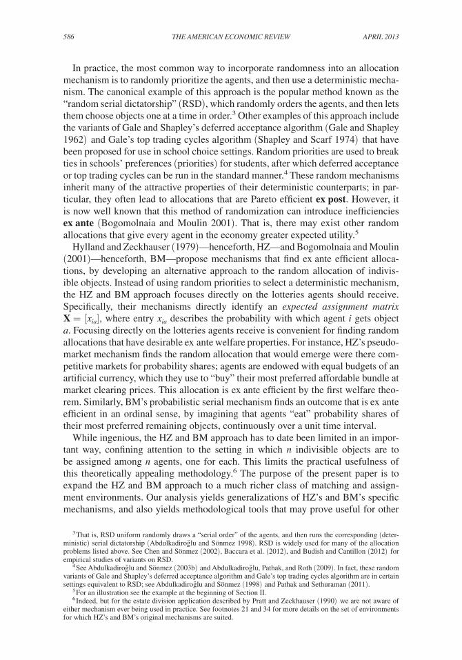
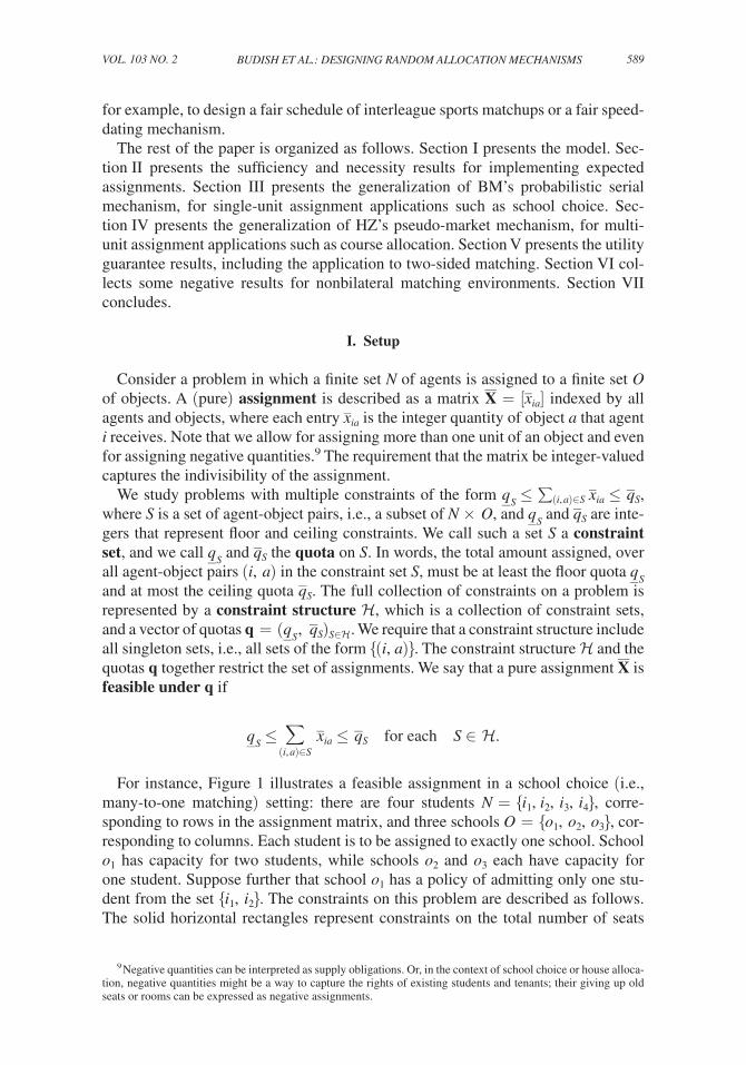
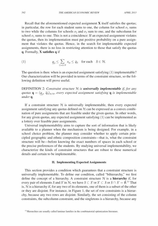
For instance, Figure 1 illustrates a feasible assignment in a school choice (i.e., many-to-one matching) setting: there are four students N = { i 1 , i 2 , i 3 , i 4 }, corre-sponding to rows in the assignment matrix, and three schools O = { o 1 , o 2 , o 3 }, cor-responding to columns. Each student is to be assigned to exactly one school. School o 1 has capacity for two students, while schools o 2 and o 3 each have capacity for one student. Suppose further that school o 1 has a policy of admitting only one stu-dent from the set { i 1 , i 2 }. The constraints on this problem are described as follows. The solid horizontal rectangles represent constraints on the total number of seats
9 Negative quantities can be interpreted as supply obligations. Or, in the context of school choice or house alloca-tion, negative quantities might be a way to capture the rights of existing students and tenants; their giving up old seats or rooms can be expressed as negative assignments.
590 THE AMERICAN ECONOMIC REVIEW ApRIl 2013
assigned to each student; we call these “row constraints.” Formally, these are the sets {i} × O for each agent i ∈ N, and have quotas q _
S = _ q S = 1. The dotted vertical
rectangles represent constraints on the number of students that can be assigned to each school; we call these “column constraints.” Formally, these are the sets N × {a} for each object a ∈ O; the first column has quotas q _
S = _ q S = 2, while the other two
columns have quotas q _ S = _ q S = 1. The group-specific constraint is represented by
the solid rectangle containing the subcolumn—the first two entries in the first col-umn—more formally by a set S = {( i 1 , o 1 ), ( i 2 , o 1 )}, with quota q _
S = _ q S = 1. Not
pictured are the constraints on each singleton set, i.e., on the number of times a specific school a is assigned to a specific student i; for the singleton sets the relevant quotas are q _ {(i, a)} = 0 and
_ q {(i, a)} = 1. The constraint structure consists of all the
row, column, subcolumn and singleton constraints. The assignment __
X depicted in Figure 1 is feasible because it satisfies the quotas q associated with each constraint set in the overall constraint structure . In words,
__ X assigns students i 1 and i 3 to
school o 1 , student i 2 to school o 2 , and student i 4 to school o 3 .Throughout the paper we will give numerous additional examples of constraint
sets and constraint structures; see especially Section IIA. As in the preceding exam-ple, most of our applications involve constraint structures with two basic groups of constraints. One group of constraints consists of sets that are columns, subsets of columns, and supersets of columns, and represents constraints on the assignment from the perspective of the objects. For example, a constraint set consisting of a subset of a column could be used to represent affirmative action constraints in the context of school choice. The constraint set would consist of all students of a par-ticular gender, race, or socioeconomic status; the quotas on that constraint set would then represent the minimum and maximum number of students from that group that could be enrolled in the school represented by that column. The second group of constraints consists of sets that are rows, subsets of rows, and supersets of rows, and represents constraints on the assignment from the perspective of the agents. For example, in course allocation, a row constraint would represent the total number of courses a student can take, while a subrow constraint might limit the number of finance courses the student can take.
Given a constraint structure and associated quotas q, a random allocation can be described as a lottery over pure assignments each of which is feasible under quotas q. As with HZ and BM, however, our approach is to focus directly on the expected assignment matrix as the basic unit of analysis. Formally, an expected assignment
1 0 0
0 1 0
1 0 0
0 0 1
X = ( ).
Figure 1. A Feasible Assignment
591budish et al.: designing random allocation mechanismsVol. 103 no. 2
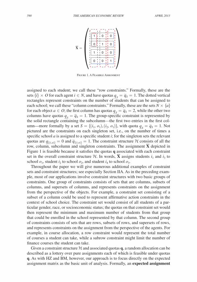
is a matrix X = [ x ia ] indexed by agents and objects where x ia ∈ (−∞, ∞) for every i ∈ N and a ∈ O.10 In contrast to pure assignment matrices, an expected assignment allows for fractional allocations of objects. One possible expected assignment in the four-students three-schools example is
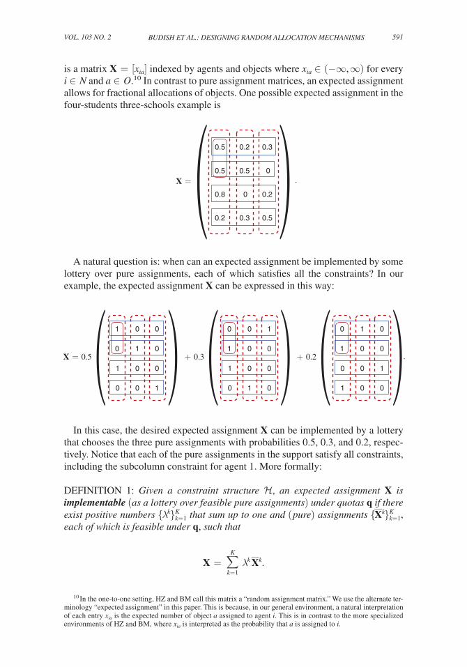
A natural question is: when can an expected assignment be implemented by some lottery over pure assignments, each of which satisfies all the constraints? In our example, the expected assignment X can be expressed in this way:
In this case, the desired expected assignment X can be implemented by a lottery that chooses the three pure assignments with probabilities 0.5, 0.3, and 0.2, respec-tively. Notice that each of the pure assignments in the support satisfy all constraints, including the subcolumn constraint for agent 1. More formally:
DEFINITION 1: Given a constraint structure , an expected assignment X is implementable (as a lottery over feasible pure assignments) under quotas q if there exist positive numbers { λ k } k=1 K
that sum up to one and ( pure) assignments { __
X k } k=1 K ,
each of which is feasible under q, such that
X = ∑ k=1
K
λ k __
X k .
10 In the one-to-one setting, HZ and BM call this matrix a “random assignment matrix.” We use the alternate ter-minology “expected assignment” in this paper. This is because, in our general environment, a natural interpretation of each entry x ia is the expected number of object a assigned to agent i. This is in contrast to the more specialized environments of HZ and BM, where x ia is interpreted as the probability that a is assigned to i.
0.5 0.2 0.3
0.5 0.5 0
0.8 0 0.2
0.2 0.3 0.5
X = ( ) .
1 0 0
0 1 0
1 0 0
0 0 1
0 0 1
1 0 0
1 0 0
0 1 0
0 1 0
1 0 0
0 0 1
1 0 0
X + 0.2 ( )X + 0.3 ( )X = 0.5 ( ) .
592 THE AMERICAN ECONOMIC REVIEW ApRIl 2013
Recall that the aforementioned expected assignment X itself satisfies the quotas; in particular, the row for each student sums to one, the column for school o 1 sums to two while the columns for schools o 2 and o 3 sum to one, and the subcolumn for school o 1 sums to one. This is not a coincidence: If an expected assignment violates the quotas, then its implementation must put positive probability on a pure assign-ment that violates the quotas. Hence, in the search for implementable expected assignments, there is no loss in restricting attention to those that satisfy the quotas q. Formally, X satisfies q if
(1) q _ S ≤ ∑
(i, a)∈S
x ia ≤ _ q S for each S ∈ .
The question is then: when is an expected assignment satisfying (1) implementable? Our characterization will be provided in terms of the constraint structure, so the fol-lowing definition will prove useful.
DEFINITION 2: Constraint structure is universally implementable if, for any quotas q = ( q _
S , _ q S ) S∈ , every expected assignment satisfying q is implementable
under q.
If a constraint structure is universally implementable, then every expected assignment satisfying any quotas defined on can be expressed as a convex combi-nation of pure assignments that are feasible under the given quotas. In other words, for any given quotas, any expected assignment satisfying (1) can be implemented as a lottery over feasible pure assignments.
Universal implementability aims to capture the sort of information that is likely available to a planner when the mechanism is being designed. For example, in a school choice problem, the planner may consider whether to apply certain prin-cipled geographic and ethnic composition constraints—that is, what the constraint structure will be—before knowing the exact numbers of spaces in each school or the precise preferences of the students. By studying universal implementability, we characterize the kinds of constraint structures that are robust to these numerical details and certain to be implementable.
II. Implementing Expected Assignments
This section provides a condition which guarantees that a constraint structure is universally implementable. To define our condition, called “bihierarchy,” we first define the concept of a hierarchy. A constraint structure is a hierarchy if, for every pair of elements S and S′ in , we have S ⊂ S′ or S′ ⊂ S or S ∩ S′ = ~.11 That is, is a hierarchy if, for any two of its elements, one of them is a subset of the other or they are disjoint. For instance, in Figure 1, the set of row constraints is a hierar-chy, because any two rows are disjoint. Similarly, the set consisting of the column constraints, the subcolumn constraint, and the singletons is a hierarchy, because any
11 Hierarchies are usually called laminar families in the combinatorial optimization literature.
593budish et al.: designing random allocation mechanismsVol. 103 no. 2
two elements in that set are either disjoint (e.g., two different columns) or have a subset relationship (e.g., the subcolumn and column corresponding to school o 1 , or a singleton and its associated column). The overall constraint structure, consisting of rows, columns, the subcolumn, and singletons, is not a hierarchy: e.g., the first row and the first column are not disjoint nor do they have a subset relationship. But, the overall constraint structure is what we call a bihierarchy, defined as follows:
DEFINITION 3: A constraint structure is a bihierarchy if there exist hierarchies 1 and 2 such that = 1 ∪ 2 and 1 ∩ 2 = ~.
In words, a bihierarchy is a constraint structure that can be expressed as the union of two disjoint hierarchies. Note that the partition of into 1 and 2 need not be unique. For instance, in Figure 1, the singleton sets in the constraint structure could be placed in the row hierarchy instead of the column hierarchy, or in fact could be divided between the two hierarchies in any arbitrary fashion. Several other examples of bihierarchies will be provided in Section IIA.
Our first result, which follows readily from the combinatorial optimization literature, establishes that the bihierarchy condition is sufficient for universal implementability.
THEOREM 1 (Sufficiency): If a constraint structure is a bihierarchy, then it is uni-versally implementable.
PROOF: Suppose that constraint structure is a bihierarchy. Consider any expected assign-
ment X that satisfies q given constraint structure . Since q _ S and
_ q S are integers for
each S ∈ , we must have q _ S ≤ ⌊ x S ⌋ ≤ x S ≤ ⌈ x S ⌉ ≤ _ q S , where x S := ∑ (i, a)∈S x ia ,
⌊ x S ⌋ is the largest integer no greater than x S , and ⌈ x S ⌉ is the smallest integer no less than x S . Hence, X must belong to the set
(2) { X′ = [ x′ ia ] | ⌊ x S ⌋ ≤ ∑ (i, a)∈S
x′ ia ≤ ⌈ x S ⌉, ∀S ∈ } .The set (2) forms a bounded polytope. Hence, any point of it, including X, can be written as a convex combination of its vertices. To prove the result, therefore, it suffices to show that the vertices of (2) are integer-valued. Hoffman and Kruskal (1956) show that the vertices of (2) are integer-valued if and only if the incidence matrix Y = [ y (i, a), S ], (i, a) ∈ N × O, S ∈ , where y (i, a), S = 1 if (i, a) ∈ S and y (i, a), S = 0 if (i, a) ∉ S, is totally unimodular.12 Finally, the stated result follows since the bihierarchical structure of implies the total unimodularity of matrix Y (Edmonds 1970). A fuller self-contained proof is available in online Appendix A.
As is clear from the proof, the pure assignments used in the implementing lot-tery in Theorem 1 not only are feasible under the given quotas; in addition, the
12 A zero-one matrix is totally unimodular if the determinant of every square submatrix is 0, −1, or +1.
594 THE AMERICAN ECONOMIC REVIEW ApRIl 2013
implementation ensures that each of the resulting pure assignments is rounded up or down to the nearest integer for each constraint set, which is a stronger property.
For practical purposes, knowing simply that an expected assignment is imple-mentable is not satisfactory; implementation must be computable, preferably by a fast algorithm. Fortunately, there exists an algorithm, formally described in online Appendix B, that implements expected assignments in polynomial time.13 At each step of the algorithm, an expected assignment X satisfying the given quotas is decomposed into a convex combination γX′ + (1 − γ)X″ of two expected assign-ments, X′ and X″, each of which satisfies the quotas and is closer to being a pure assignment in the following sense: every constraint set S ∈ that is integer valued in X (i.e., ∑(i, a)∈S x ia ∈ 핑) remains integer valued in both X′ and X″, and there is at least one additional integer valued constraint set in both X′ and X″. Then, a random number is generated and with probability γ the algorithm continues by similarly decomposing X′, while with probability 1 − γ the algorithm continues by decom-posing X″. The algorithm stops when it reaches a pure assignment. As argued more formally in the Appendix, this process has a run time polynomial in | |.
A. Examples of Bihierarchy
In this section we provide several examples of constraint structures that satisfy the bihierarchy condition, and are thus universally implementable per Theorem 1.
One-to-One Assignment and the Birkhoff-von Neumann Theorem.—Suppose n agents are to be assigned n objects, one for each. Notice that any pure assignment is described as an n × n permutation matrix; namely, each entry is zero or one, each row sums to one, and each column sums to one. Any expected assignment is in turn represented as an n × n bistochastic matrix, i.e., a matrix with entries in [0, 1], sat-isfying the same row-sum and column-sum constraints. The Birkhoff-von Neumann theorem states that any bistochastic matrix can be expressed as a convex combina-tion of permutation matrices. Clearly, this result follows from Theorem 1; all rows are disjoint and thus form a hierarchy, and all columns form another. (Singletons can be added arbitrarily to either hierarchy.)
COROLLARY 1 (Birkhoff 1946; von Neumann 1953): Every bistochastic matrix is a convex combination of permutation matrices.
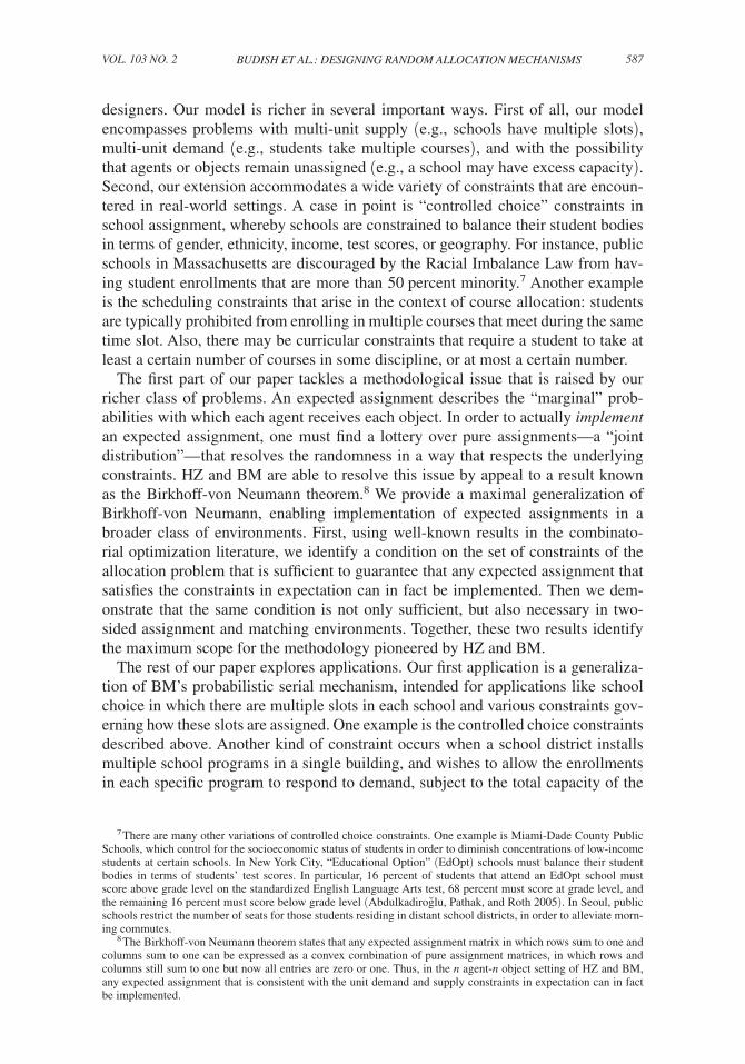
Endogenous Capacities.—Consider a school choice problem in which the school authority wishes to run several education programs within one school building. An assignment in such an environment can be described as a matrix in which rows cor-respond to students and columns correspond to education programs; each school building then corresponds to multiple columns. Formally, we can let 1 include all rows, while 2 includes all columns, as well as sets of the form N × O′, where O′ corresponds to multiple educational programs that share a building. The ceiling _ q N×{a} describes the total number of students who can be admitted to program a,
13 We thank Tomomi Matsui and Akihisa Tamura for suggesting the algorithm. An earlier draft of this paper included an alternative algorithm generalizing the stepping-stones algorithm described by HZ.

595budish et al.: designing random allocation mechanismsVol. 103 no. 2
while the ceiling _ q N× O ′ describes the total capacity of the building housing the pro-
grams in O′. If the sum of ceilings ∑a∈ O ′ _ q N×{a} is larger than the ceiling
_ q N× O ′ ,
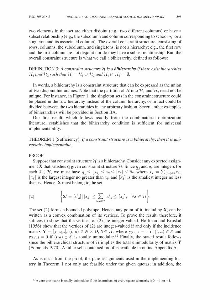
then that means the sizes of programs within the school building can be adjusted, subject to the building’s overall (say, physical) capacity. For instance, in Figure 2, columns b and c represent two programs within a school each of which is subject to a quota, and there is a school-wide quota impinging on b and c, together. Since each school program belongs to just one building, the constraint structure 2 is a hierar-chy, hence 1 ∪ 2 is a bihierarchy and is universally implementable.
Group-Specific Quotas.—Affirmative action policies are sometimes implemented as quotas on students of a specific gender, race, or socioeconomic status.14 A similar mathematical structure results from New York City’s Educational Option programs, which achieve a mix of students by imposing quotas on students with various test scores (Abdulkadiro ̆ g lu, Pathak, and Roth 2005). Quotas may also be based on the residence of applicants: The school choice program of Seoul, Korea, limits the per-centage of seats allocated to applicants from outside the district.15 A number of school choice programs in Japan have similar quotas based on residential areas as well.
As above, let 1 include all rows, which correspond to students, and let 2 include all columns, which correspond to schools. Group-specific quotas can be handled by including “subcolumns” in 2 ; formally a subcolumn is a set of the form N′ × {a} for a ∈ O and N′ ⊊ N. The ceiling
_ q N ′ ×{a} then determines the maximum number
of students school a can admit from group N′. Quotas on multiple groups can be imposed for each a without violating the hierarchy structure as long as they do not overlap with each other.16 For instance, in Figure 2, school a has a maximum quota
14 Abdulkadiro ̆ g lu and Sönmez (2003b) and Abdulkadiro ̆ g lu (2005) analyze assignment mechanisms under affirmative action constraints.
15 See “Students’ High School Choice in Seoul Outlined,” Digital Chosun Ilbo, October 16, 2008 (http://english.chosun.com/site/data/html_dir/2008/10/16/2008101661016.html (accessed January 18, 2013)).
16 In fact, some overlap of constraint sets can be accommodated with a small error. Suppose a school has maxi-mal quotas for white and male at 60 and 55, respectively. Suppose an expected assignment assigns 40.5 white male, 14.5 black male, and 19.5 white female students to that school. Notice both ceilings are binding at this expected assignment. This expected assignment can be implemented recognizing only white and male, white and female, and male as the constraint sets, which then forms a hierarchy. Implementing with this modified constraint structure may violate the maximal quota for whites, since the constraint set for “white” is not included in the structure; for instance, the school may get 41 white male, 14 black male, and 20 white female students. However, the violation is by only one student. In fact, the degree of violation is at most one when there is only one overlap of constraint
( )x1a x1b x1c
x2a x2b x2c
x3a x3b x3c
Figure 2. Endogenous Capacities and Group-Specific Quotas
596 THE AMERICAN ECONOMIC REVIEW ApRIl 2013
for its student body (entire column) but also has a maximum quota on a particular group of students represented by rows 1 and 2 (dashed subcolumn). Moreover, a nested series of constraints can be accommodated. For instance, a school system can require that a school admit at most 50 students from district one, at most 50 students from district two, and at most 80 students from either district one or two.
It is also possible to accommodate both flexible-capacity constraints and group-specific quota constraints within the same hierarchy 2 . Flexible-capacity con-straints are defined on multiple columns of an expected assignment matrix X, whereas group-specific quota constraints are defined on subsets of single columns of X. Any subset of a single column will be a subset of or disjoint from any set of multiple columns. Figure 2 provides an illustration.
Course Allocation.—In course allocation, each student may enroll in multiple courses, but cannot receive more than one seat in any single course. Moreover, each student may have preference or feasibility constraints that limit the number of courses taken from certain sets. For example, scheduling constraints prohibit any student from taking two courses that meet during the same time slot. Or, a student might prefer to take at most two courses on finance, at most three on marketing, and at most four on finance or marketing in total.
Many such restrictions can be modeled using a bihierarchy, with 1 including all rows and 2 including all columns. Setting
_ q {(i, a)} = 1 and
_ q {i}×O > 1 for each i ∈ N
and a ∈ O ensures that each student i can enroll in multiple courses but receive at most one seat in each course. Letting F and M be the sets of finance courses and mar-keting courses, respectively, if 1 contains {i} × F, {i} × M, and {i} × (F ∪ M ), then we can express the constraints “student i can take at most
_ q {i}×F courses in
finance, _ q {i}×M courses in marketing, and
_ q {i}×(F∪M ) in finance and marketing com-
bined.” Scheduling constraints are handled similarly; for instance, F and M can be sets of classes offered at different times (e.g., Friday morning and Monday morn-ing). It may be impossible, however, to express both subject and scheduling con-straints while still maintaining a bihierarchical constraint structure.
Note that the flexible production and group-specific quota constraints described in Section IIA can also be incorporated into the course allocation problem without jeopardizing the bihierarchical structure. These constraints can be included in 2 , while the preference and scheduling constraints described above can be included in 1 . So long as 1 and 2 are both hierarchies, = 1 ∪ 2 is a bihierarchy.
Interleague Play Matchup Design.—Our framework can also be applied to match-ing problems, in which N and O are both sets of agents, and entry (i, a) in the assign-ment matrix represents whether (and, in some applications, how many times) i is matched with a. As an example, consider sports scheduling. Many professional sports associations, including Major League Baseball (MLB) and the National Football League (NFL), have two separate leagues. In MLB, teams in the American League (AL) and National League (NL) had traditionally played against teams only
sets. Such a small violation can often be tolerated in realistic controlled-choice environments. In case the quotas are rigid, the quota can be set more conservatively; for instance in the above example, the quota for whites can be set at 59 instead of 60.
597budish et al.: designing random allocation mechanismsVol. 103 no. 2
within their own league during the regular season, but play across the AL and NL, called interleague play, was introduced in 1997.17 Unlike the intraleague games, the number of interleague games is relatively small, and this can make the indivisibility problem particularly difficult to deal with in designing the matchups.
For example, suppose there are two leagues, N and O, each with nine teams. Suppose each team must play 15 games against teams in the other league. This can be represented by forming a 9 × 9 matrix where entry (i, a) corresponds to the num-ber of times team i ∈ N plays team a ∈ O. The constraint that each team must play 15 games against teams in the other leagues can be handled by adding all row and column constraints, each with floor and ceiling set equal to 15. Ignoring indivisibility, a fair matchup will require each team in one league to play every team in the other league the same number of times, that is, 15/9 ≈ 1.67 times. Of course, this frac-tional matchup itself is infeasible, but one can implement this expected matchup as a convex combination of feasible matchups. In doing so, one can also specify additional constraints: e.g., each team in N has a geographic rival in O and they must play at least once; or, teams in each league must face opponents in the other league of similar difficulty. Specifically, one could require each team to play at least four games with the top three teams, four games with the middle three teams, and four games with the bottom three teams of the other league, by adding the appropriate subrow and subcol-umn constraints. Our approach can produce a feasible matchup that implements the uniform expected assignment while also satisfying these additional constraints.
B. Necessity of a Bihierarchical Constraint Structure
Theorem 1 shows that bihierarchy is sufficient for universal implementability. This section identifies a sense in which it is also necessary. Doing so also provides an intuition about the role bihierarchy plays for implementation of expected assign-ments. We begin with an example of a non-bihierarchical constraint structure that is not universally implementable.
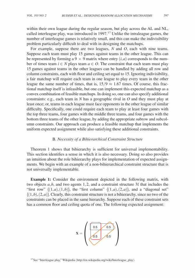
Example 1: Consider the environment depicted in the following matrix, with two objects a, b, and two agents 1, 2, and a constraint structure that includes the “first row” {(1, a), (1, b)}, the “first column” {(1, a), (2, a)}, and a “diagonal set” {(1, b), (2, a)}. Clearly, this constraint structure is not a bihierarchy, since no two of the constraints can be placed in the same hierarchy. Suppose each of these constraint sets has a common floor and ceiling quota of one. The following expected assignment:
17 See “Interleague play,” Wikipedia (http://en.wikipedia.org/wiki/Interleague_play).
0.5
0.5
0.5
0.5X = ( )

598 THE AMERICAN ECONOMIC REVIEW ApRIl 2013
satisfies the quotas, but it cannot be implemented as a lottery over feasible pure assignments.18 To see this, first observe that the lottery implementing X must choose with positive probability a pure assignment
__ X in which
_ x 1a = 1. Since the first row
has a quota of one, it follows that _ x 1b = 0. Since the diagonal set has a quota of one,
it follows that _ x 2a = 1. This is a contradiction because the quota for the first column
is violated at __
X since _ x {(1, a),(2, a)} = _ x 1a + _ x 2a = 2.
Is bihierarchy necessary for universal implementability? It turns out this is not the case.19 Yet, we now show that bihierarchy implies universal implementability for an important class of constraint structures. In two-sided assignment problems, there are often quotas for each individual agent and quotas for each object. We say that is a canonical two-sided constraint structure if contains all “rows” (i.e., sets of the form {i} × O for each i ∈ N ) and all “columns” (i.e., sets of the form N × {a} for each a ∈ O). The next result demonstrates that bihierarchy is necessary for universal implementability for such constraint structures.
THEOREM 2 (Necessity): If a canonical two-sided constraint structure is not a bihierarchy, then it is not universally implementable.
The formal proof of Theorem 2 is in the online Appendix. The proof shows that whenever a canonical two-sided constrained structure fails to be a bihierarchy one can always find an expected assignment and quotas that lead to the situation much like that of Example 1. (See Section VI for a necessary condition for universal implementability that generalizes the idea behind Example 1.) Thus, in the context of typical two-sided assignment and matching problems, bihierarchy is both neces-sary and sufficient for universal implementability. We now turn to applications.
III. A Generalization of the Probabilistic Serial Mechanism for Assignment with Single-Unit Demand
In this section, we consider the problem of assigning indivisible objects to agents who can consume at most one object each. Examples include university housing allocation, public housing allocation, office assignment, and student placement in public schools.
18 Notationally, the convention throughout the paper is that the ith row of the expected assignment matrix from the top corresponds to agent i while the first column from the left corresponds to object a, the second column cor-responds to object b, and so on.
19 To see that bihierarchy is not necessary, consider an environment with two objects and two agents as before, but let
= {{(1, a), (1, b)}, {(1, a), (2, a)}, {(1, a), (2, b)}},and the floor and ceiling quotas for each constraint set be one. Note is not a bihierarchy. Yet, any expected assignment
X = ( s t
t t ) ,
with s + t = 1, can be decomposed by a convex combination of pure assignments as
X = ( s t
t t ) = s (
1 0
0 0 ) + t (
0 1
1 1 ) .
599budish et al.: designing random allocation mechanismsVol. 103 no. 2
A common method for allocating objects in such a setting is the random serial dictatorship. In this mechanism, every agent reports preference rankings of the objects. The mechanism designer then randomly orders the agents with equal prob-ability. The first agent in the realized order receives her stated favorite (most pre-ferred) object, the next agent receives her stated favorite object among the remaining ones, and so on. The random serial dictatorship is strategy-proof, that is, reporting preferences truthfully is a weakly dominant strategy for every agent. Moreover, the random serial dictatorship is ex post efficient, that is, every pure assignment that occurs with positive probability under the mechanism is Pareto efficient.
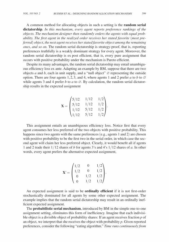
Despite its many advantages, the random serial dictatorship may entail unambigu-ous efficiency loss ex ante. Adapting an example by BM, suppose that there are two objects a and b, each in unit supply, and a “null object” ∅ representing the outside option. There are four agents 1, 2, 3, and 4, where agents 1 and 2 prefer a to b to ∅ while agents 3 and 4 prefer b to a to ∅. By calculation, the random serial dictator-ship results in the expected assignment
X = ( 5/12
5/12 1/12
1/12
1/12
1/12 5/12
5/12
1/2
1/2 1/2
1/2
).
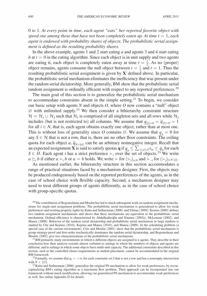
This assignment entails an unambiguous efficiency loss. Notice first that every agent consumes her less preferred of the two objects with positive probability. This happens since two agents with the same preferences (e.g., agents 1 and 2) are chosen with positive probability to be the first two in the serial order, in which case the sec-ond agent will claim her less preferred object. Clearly, it would benefit all if agents 1 and 2 trade their 1/12 shares of b for agents 3’s and 4’s 1/12 shares of a. In other words, every agent prefers the alternative expected assignment,
X′ = ( 1/2
1/2 0
0
0
0 1/2
1/2
1/2
1/2 1/2
1/2
).
An expected assignment is said to be ordinally efficient if it is not first-order stochastically dominated for all agents by some other expected assignment. The example implies that the random serial dictatorship may result in an ordinally inef-ficient expected assignment.
The probabilistic serial mechanism, introduced by BM in the simple one-to-one assignment setting, eliminates this form of inefficiency. Imagine that each indivisi-ble object is a divisible object of probability shares: If an agent receives fraction p of an object, we interpret that she receives the object with probability p. Given reported preferences, consider the following “eating algorithm.” Time runs continuously from
600 THE AMERICAN ECONOMIC REVIEW ApRIl 2013
0 to 1. At every point in time, each agent “eats” her reported favorite object with speed one among those that have not been completely eaten up. At time t = 1, each agent is endowed with probability shares of objects. The probabilistic serial assign-ment is defined as the resulting probability shares.
In the above example, agents 1 and 2 start eating a and agents 3 and 4 start eating b at t = 0 in the eating algorithm. Since each object is in unit supply and two agents are eating it, each object is completely eaten away at time t = 1 _ 2 . As no (proper) object remains, agents consume the null object between t = 1 _ 2 and t = 1. Thus the resulting probabilistic serial assignment is given by X′ defined above. In particular, the probabilistic serial mechanism eliminates the inefficiency that was present under the random serial dictatorship. More generally, BM show that the probabilistic serial random assignment is ordinally efficient with respect to any reported preferences.20
The main goal of this section is to generalize the probabilistic serial mechanism to accommodate constraints absent in the simple setting.21 To begin, we consider our basic setup with agents N and objects O, where O now contains a “null” object ∅ with unlimited supply.22 We then consider a bihierarchy constraint structure = 1 ∪ 2 such that 1 is comprised of all singleton sets and all rows while 2 includes (but is not restricted to) all columns. We assume that q _ {i}×O = _ q {i}×O = 1 for all i ∈ N, that is, each agent obtains exactly one object, rather than at most one. This is without loss of generality since O contains ∅. We assume that q _ S = 0 for any S ∈ that is not a row, that is, there are no other floor constraints. The ceiling quota for each object a,
_ q N×{a} , can be an arbitrary nonnegative integer. Recall that
an expected assignment X is said to satisfy quotas q if q _ S ≤ ∑ (i, a)∈S
x ia ≤ _ q S for each
S ∈ H. Each agent i has a strict preference ≻ i over the set of objects.23 We write a ⪰ i b if either a ≻ i b or a = b holds. We write ≻ for ( ≻ i ) i∈N and ≻ −i for ( ≻ j ) j∈N \{i} .
As mentioned earlier, the bihierarchy structure in this section accommodates a range of practical situations faced by a mechanism designer. First, the objects may be produced endogenously based on the reported preferences of the agents, as in the case of school choice with flexible capacity. Second, a mechanism designer may need to treat different groups of agents differently, as in the case of school choice with group-specific quotas.
20 The contribution of Bogomolnaia and Moulin has led to much subsequent work on random assignment mecha-nisms for single-unit assignment problems. The probabilistic serial mechanism is generalized to allow for weak preferences and existing property rights by Katta and Sethuraman (2006) and Yilmaz (2009). Kesten (2009) defines two random assignment mechanisms and shows that these mechanisms are equivalent to the probabilistic serial mechanism. Ordinal efficiency is characterized by Abdulkadiro ̆ g lu and Sönmez (2003a), McLennan (2002), and Manea (2008). Behavior of the random serial dictatorship and probabilistic serial mechanism in large markets is studied by Che and Kojima (2010), Kojima and Manea (2010), and Manea (2009). In the scheduling problem (a special case of the current environment), Crès and Moulin (2001) show that the probabilistic serial mechanism is group strategy-proof and first-order stochastically dominates the random serial dictatorship, and Bogomolnaia and Moulin (2002) give two characterizations of the probabilistic serial mechanism.
21 BM primarily study environments in which n different objects are assigned to n agents. They describe in their conclusion how their analysis extends almost verbatim to settings in which the numbers of objects and agents are different, and to settings in which some objects have multi-unit capacity. The additional constraints described in this section, such as the controlled choice requirements in student placement, cannot be accommodated in the original BM framework.
22 Formally, we assume that _ q S = +∞ for each constraint set S that is not a row and has a nonempty intersection
with N × {∅}.23 Katta and Sethuraman (2006) generalize the original PS mechanism to allow for weak preferences, by recon-
ceptualizing BM’s eating algorithm as a maximum flow problem. Their approach can be incorporated into our framework without much modification, allowing our generalized PS mechanism to accommodate weak preferences as well. See online Appendix D for details.
601budish et al.: designing random allocation mechanismsVol. 103 no. 2
Now we introduce the generalized probabilistic serial mechanism. As in BM, the basic idea is to regard each indivisible object as a divisible object of “ probability shares.” More specifically, the algorithm is described as follows: Time runs continu-ously from 0 to 1. At every point in time, each agent “eats” her reported favorite object with speed one among those that are “available” at that instance, and the probabilistic serial assignment is defined as the probability shares eaten by each agent by time 1. In order to obtain an implementable expected assignment in the presence of additional constraints, however, we modify the definition of “available.” More specifically, we say that object a is “available” to agent i if and only if, for every constraint set S such that (i, a) ∈ S, the total amount of consumption over all agent-object pairs in S is strictly less than its ceiling quota
_ q S . This algorithm
is formally defined in Appendix A. Given reported preferences ≻, the generalized probabilistic serial assignment is denoted PS(≻).
Note that two modifications are made in the definition of the algorithm from the version of BM. First, we specify availability of objects with respect to both agents and objects in order to accommodate complex constraints such as con-trolled choice. Second, we need to keep track of multiple constraints for each agent-object pair (i, a) during the algorithm, since there are potentially multiple constraints that would make the consumption of object a by agent i no longer feasible.
Since the constraint structure in this section is a bihierarchy, and the general-ized PS mechanism always produces an expected assignment that satisfies the given quotas, Theorem 1 implies that the resulting expected assignment is always implementable:
COROLLARY 2: For any preference profile ≻, the generalized probabilistic serial assignment PS(≻) is implementable.
PROOF: The result follows immediately from Theorem 1, because the constraint structure
under consideration forms a bihierarchy and PS(≻) satisfies all quotas associated with that constraint structure by construction.
In this sense, the mechanism is well-defined as an expected assignment mecha-nism in the current setting. The following example illustrates how the mechanism works.
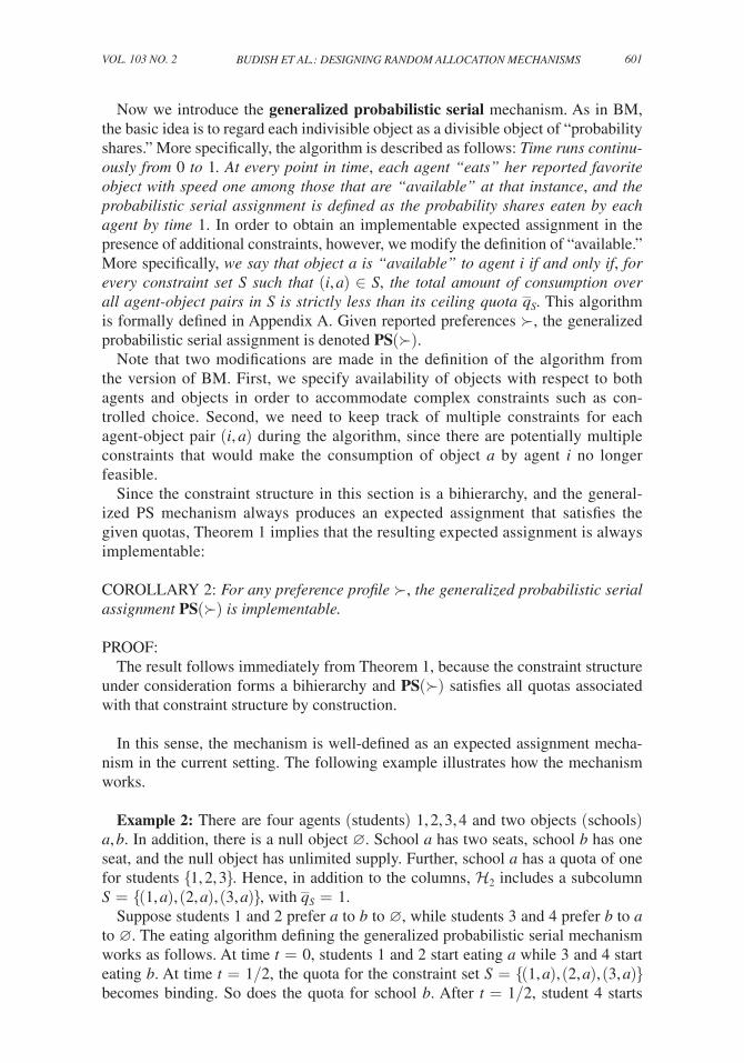
Example 2: There are four agents (students) 1, 2, 3, 4 and two objects (schools) a, b. In addition, there is a null object ∅. School a has two seats, school b has one seat, and the null object has unlimited supply. Further, school a has a quota of one for students {1, 2, 3}. Hence, in addition to the columns, 2 includes a subcolumn S = {(1, a), (2, a), (3, a)}, with
_ q S = 1.
Suppose students 1 and 2 prefer a to b to ∅, while students 3 and 4 prefer b to a to ∅. The eating algorithm defining the generalized probabilistic serial mechanism works as follows. At time t = 0, students 1 and 2 start eating a while 3 and 4 start eating b. At time t = 1/2, the quota for the constraint set S = {(1, a), (2, a), (3, a)} becomes binding. So does the quota for school b. After t = 1/2, student 4 starts
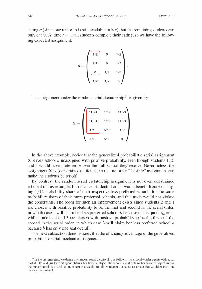
602 THE AMERICAN ECONOMIC REVIEW ApRIl 2013
eating a (since one unit of a is still available to her), but the remaining students can only eat ∅. At time t = 1, all students complete their eating, so we have the follow-ing expected assignment:
1/2
1/2
1/2
1/2
1/2
1/2 1/2
1/2
0
0
0
0
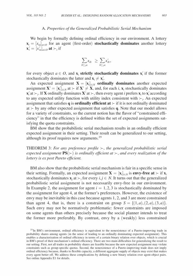
X = ( ) .The assignment under the random serial dictatorship24 is given by
11/24
11/24
11/24
11/24
1/2
7/12 5/12
5/12
1/12
1/12
1/12
0
X′ = ( ) .In the above example, notice that the generalized probabilistic serial assignment
X leaves school a unassigned with positive probability, even though students 1, 2, and 3 would have preferred a over the null school they receive. Nevertheless, the assignment X is (constrained) efficient, in that no other “feasible” assignment can make the students better off.
By contrast, the random serial dictatorship assignment is not even constrained efficient in this example: for instance, students 1 and 3 would benefit from exchang-ing 1/12 probability share of their respective less preferred schools for the same probability share of their more preferred schools, and this trade would not violate the constraints. The room for such an improvement exists since students 2 and 1 are chosen with positive probability to be the first and second in the serial order, in which case 1 will claim her less preferred school b because of the quota
_ q S = 1,
while students 4 and 3 are chosen with positive probability to be the first and the second in the serial order, in which case 3 will claim her less preferred school a because b has only one seat overall.
The next subsection demonstrates that the efficiency advantage of the generalized probabilistic serial mechanism is general.
24 In the current setup, we define the random serial dictatorship as follows: (i) randomly order agents with equal probability, and (ii) the first agent obtains her favorite object, the second agent obtains her favorite object among the remaining objects, and so on, except that we do not allow an agent to select an object that would cause some quota to be violated.
603budish et al.: designing random allocation mechanismsVol. 103 no. 2
A. Properties of the Generalized Probabilistic Serial Mechanism
We begin by formally defining ordinal efficiency in our environment. A lottery x i = [ x ia ] a∈O for an agent (first-order) stochastically dominates another lottery x i ′ = [ x ia ′ ] a∈O at ≻ i if
∑ b ⪰ i a
x ib ≥ ∑ b ⪰ i a
x ib ′ ,
for every object a ∈ O, and x i strictly stochastically dominates x i ′ if the former stochastically dominates the latter and x i ≠ x i ′ .
An expected assignment X = [ x i ] i∈N ordinally dominates another expected assignment X′ = [ x i ′ ] i∈N at ≻ if X′ ≠ X, and, for each i, x i stochastically dominates x i ′ at ≻ i . If X ordinally dominates X′ at ≻, then every agent i prefers x i to x i ′ according to any expected utility function with utility index consistent with ≻ i . An expected assignment that satisfies q is ordinally efficient at ≻ if it is not ordinally dominated at ≻ by any other expected assignment that satisfies q. Note that our model allows for a variety of constraints, so the current notion has the flavor of “constrained effi-ciency” in that the efficiency is defined within the set of expected assignments sat-isfying the quota constraints.
BM show that the probabilistic serial mechanism results in an ordinally efficient expected assignment in their setting. Their result can be generalized to our setting, although its proof requires new arguments.25
THEOREM 3: For any preference profile ≻, the generalized probabilistic serial expected assignment PS(≻) is ordinally efficient at ≻, and every realization of the lottery is ex post Pareto efficient.
BM also show that the probabilistic serial mechanism is fair in a specific sense in their setting. Formally, an expected assignment X = [ x i ] i∈N is envy-free at ≻ if x i stochastically dominates x j at ≻ i for every i, j ∈ N. It turns out that the generalized probabilistic serial assignment is not necessarily envy-free in our environment. In Example 2, the assignment for agent i = 1, 2, 3 is stochastically dominated by the assignment for agent 4, at the former’s preferences. However, the existence of envy may be inevitable in this case because agents 1, 2, and 3 are more constrained than agent 4, that is, there is a constraint on group S = {(1, a), (2, a), (3, a)}. Such envy may not be normatively problematic: fewer constraints are imposed on some agents than others precisely because the social planner intends to treat the former more preferably. By contrast, envy by a (weakly) less constrained
25 In BM’s environment, ordinal efficiency is equivalent to the nonexistence of a Pareto-improving trade in probability shares among agents (in the sense of leading to an ordinally dominating expected assignment). This enables a characterization of ordinal efficiency in terms of a certain binary relation over objects, which is crucial in BM’s proof of their mechanism’s ordinal efficiency. There are two main difficulties for generalizing the result to our setting. First, not all trades in probability shares are feasible because the new expected assignment may violate constraints such as group-specific quotas. Second, the nonexistence of a Pareto-improving trade does not imply ordinal efficiency because, thanks to flexible capacity, a different aggregate supply of objects may exist that makes every agent better off. We address these complications by defining a new binary relation over agent-object pairs. See online Appendix E1 for details.
604 THE AMERICAN ECONOMIC REVIEW ApRIl 2013
agent of a (weakly) more constrained agent is normatively more problematic. In Example 2, no such envy exists; each of agents 1, 2, and 3 prefers her own assign-ment to the others in this group, and agent 4 prefers her own assignment to those of any other agent. To formalize this idea, say agent i weakly envies agent j at X = [ x i ] i∈N at ≻ if x i does not stochastically dominate x j at the former’s prefer-ence. We say an expected assignment X = [ x i ] i∈N is constrained envy-free at ≻ if whenever i weakly envies j in X, there exists S ∈ 2 binding in X (i.e., x S = _ q S ) such that (i, a) ∈ S but ( j, a) ∉ S, for some a ∈ O.26 In words, constrained envy- freeness requires that an agent can never even weakly envy another if there is no binding constraint on a set in 2 that only the former faces. This means in par-ticular that if agent i faces constraints in 2 that are weak subsets of agent j ’s, then agent i cannot weakly envy agent j. In the above example, the outcome of the generalized probabilistic serial is constrained envy-free. This observation is generalized as follows.27
THEOREM 4: For any preference profile ≻, the generalized probabilistic serial expected assignment PS(≻) is constrained envy-free at ≻.
Two remarks are worth making. First, Theorem 4 obviously means that those facing the same constraints have no envy of each other. This means that if no group specific constraints are present (i.e., all constraints in 2 involve full columns), then the generalized probabilistic serial assignment satisfies the standard notion of envy-freeness. Second, the random serial dictatorship also admits the same type of envy as the generalized probabilistic serial mechanism. This can be seen in Example 2 where agents 1, 2, and 3 all envy agent 4 (in the sense of stochastic dominance). More importantly from the standpoint of Theorem 4, the random serial dictatorship violates even constrained envy-freeness unlike the generalized probabilistic serial mechanism: in Example 2, agent 3 weakly envies agent 1 even though both face the same constraints.
Unfortunately, the probabilistic serial mechanism is not strategy-proof, that is, there are situations in which an agent is made better off by misreporting her pref-erences. However, BM show that the probabilistic serial mechanism is weakly strategy-proof in their setting, that is, an agent cannot misstate her preferences and obtain an expected assignment that strictly stochastically dominates the one obtained under truth-telling. With some additional arguments, we can generalize their claim to our environment. Formally, we claim that the generalized probabilis-tic serial mechanism is weakly strategy-proof, that is, there exist no ≻, i ∈ N and
26 Example 2 suggests that one cannot expect the generalized probabilistic serial assignment to satisfy a stronger notion of envy-freeness. For instance, a natural notion would require that whenever an agent i envies j, exchanging their assignments must violate a constraint. Clearly, X fails this notion since agent 1 envies agent 4, and exchanging their assignments would not violate any constraints.
27 The proof is a simple adaptation of BM. For completeness, we include it in online Appendix E2.
605budish et al.: designing random allocation mechanismsVol. 103 no. 2
≻ i ′ such that P S i ( ≻ i ′ , ≻ −i ) strictly stochastically dominates P S i (≻) at ≻ i in our more general environment.28, 29
THEOREM 5: The generalized probabilistic serial mechanism is weakly strategy-proof.
One limitation of our generalization is that the algorithm is defined only for cases with maximum quotas: The minimum quota for each group must be zero. In the con-text of school choice, this precludes the administrator from requiring that at least a certain number of students from a group attend a particular school. Despite this limi-tation, administrative goals can often be sufficiently represented using maximum quotas alone.30 For instance, if there are two groups of students, “rich” and “poor,” a requirement that at least a certain number of poor students attend some highly desirable school might be adequately replaced by a maximum quota on the number of rich students who attend.
IV. A Generalization of the Pseudo-Market Mechanism for Assignment with Multi-Unit Demand
In an influential paper, HZ propose an ex ante efficient mechanism for the prob-lem of assigning n objects among n agents with single-unit demand. Based on the old idea of a competitive equilibrium from equal incomes, the mechanism can be described as follows. Agents report their von Neumann-Morgenstern preferences over individual objects. Each agent is allocated an equal budget of an artificial currency. The mechanism then computes a competitive equilibrium of this market, where the objects being priced and allocated are probability shares of objects. As the allocations are based on a competitive equilibrium, each agent is allocated a probability share profile that maximizes her expected utility subject to her bud-get constraint at the competitive equilibrium prices. This expected assignment is ex ante efficient by the first welfare theorem. It is also envy-free in the sense that each agent weakly prefers her lottery over anyone else’s according to her expected utility, because all agents have identical budget constraints. The resulting expected assignment can be implemented by appeal to the Birkhoff-von Neumann theorem.
By contrast, designing desirable mechanisms has been challenging in problems where agents have multi-unit demand, as in the assignment of course schedules to
28 As will be seen in online Appendix E3, the proof is conceptually similar to BM’s proof of weak strategy-proofness, but requires one new technical result (Lemma E.4 in the online Appendix) that shows that the effect of an agent’s preference misreport is in a certain sense small with respect to all constraint sets. In the BM environment one only needs to keep track of the time at which each object reaches capacity, whereas in our environment one needs to keep track of the time at which each constraint set (including but not limited to single-object constraints) reaches capacity.
29 Kojima and Manea (2010) show that truth-telling becomes a dominant strategy for a sufficiently large market under the probabilistic serial mechanism in a simpler environment than the current one. Showing a similar claim in our environment is beyond the scope of this paper, but we conjecture that the argument can be extended.
30 See Kojima (2012) and Hafalir, Yenmez, and Yildirim (forthcoming) on the limits of this approach. See also Ehlers et al. (2011) for an approach that accommodates floor constraints provided that they are interpreted as “soft constraints.”
606 THE AMERICAN ECONOMIC REVIEW ApRIl 2013
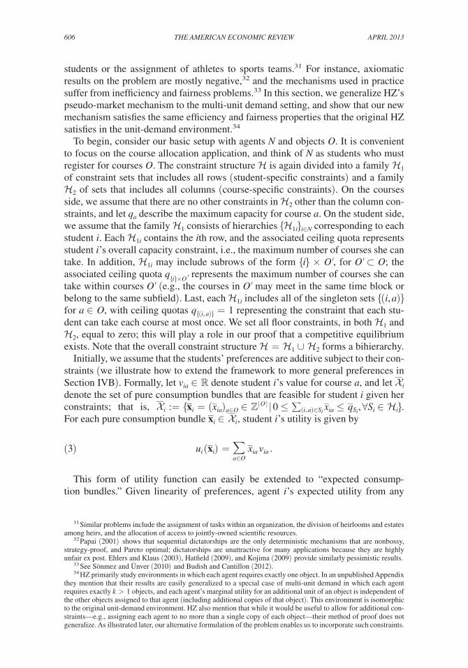
students or the assignment of athletes to sports teams.31 For instance, axiomatic results on the problem are mostly negative,32 and the mechanisms used in practice suffer from inefficiency and fairness problems.33 In this section, we generalize HZ’s pseudo-market mechanism to the multi-unit demand setting, and show that our new mechanism satisfies the same efficiency and fairness properties that the original HZ satisfies in the unit-demand environment.34
To begin, consider our basic setup with agents N and objects O. It is convenient to focus on the course allocation application, and think of N as students who must register for courses O. The constraint structure is again divided into a family 1 of constraint sets that includes all rows (student-specific constraints) and a family 2 of sets that includes all columns (course-specific constraints). On the courses side, we assume that there are no other constraints in 2 other than the column con-straints, and let q a describe the maximum capacity for course a. On the student side, we assume that the family 1 consists of hierarchies { 1i } i∈N corresponding to each student i. Each 1i contains the ith row, and the associated ceiling quota represents student i ’s overall capacity constraint, i.e., the maximum number of courses she can take. In addition, 1i may include subrows of the form {i} × O′, for O′ ⊂ O; the associated ceiling quota q {i}× O ′ represents the maximum number of courses she can take within courses O′ (e.g., the courses in O′ may meet in the same time block or belong to the same subfield). Last, each 1i includes all of the singleton sets {(i, a)} for a ∈ O, with ceiling quotas q {(i, a)} = 1 representing the constraint that each stu-dent can take each course at most once. We set all floor constraints, in both 1 and 2 , equal to zero; this will play a role in our proof that a competitive equilibrium exists. Note that the overall constraint structure = 1 ∪ 2 forms a bihierarchy.
Initially, we assume that the students’ preferences are additive subject to their con-straints (we illustrate how to extend the framework to more general preferences in Section IVB). Formally, let v ia ∈ 핉 denote student i ’s value for course a, and let
__ i
denote the set of pure consumption bundles that are feasible for student i given her constraints; that is,
__ i := { _ x i = ( _ x ia ) a∈O ∈ 핑 | O | | 0 ≤ ∑(i, a)∈ S i
_ x ia ≤ _ q S i , ∀ S i ∈ i }. For each pure consumption bundle
_ x i ∈
__ i , student i ’s utility is given by
(3) u i ( _ x i ) = ∑
a∈O
_ x ia v ia .
This form of utility function can easily be extended to “expected consump-tion bundles.” Given linearity of preferences, agent i ’s expected utility from any
31 Similar problems include the assignment of tasks within an organization, the division of heirlooms and estates among heirs, and the allocation of access to jointly-owned scientific resources.
32 Papai (2001) shows that sequential dictatorships are the only deterministic mechanisms that are nonbossy, strategy-proof, and Pareto optimal; dictatorships are unattractive for many applications because they are highly unfair ex post. Ehlers and Klaus (2003), Hatfield (2009), and Kojima (2009) provide similarly pessimistic results.
33 See Sönmez and Ünver (2010) and Budish and Cantillon (2012).34 HZ primarily study environments in which each agent requires exactly one object. In an unpublished Appendix
they mention that their results are easily generalized to a special case of multi-unit demand in which each agent requires exactly k > 1 objects, and each agent’s marginal utility for an additional unit of an object is independent of the other objects assigned to that agent (including additional copies of that object). This environment is isomorphic to the original unit-demand environment. HZ also mention that while it would be useful to allow for additional con-straints—e.g., assigning each agent to no more than a single copy of each object—their method of proof does not generalize. As illustrated later, our alternative formulation of the problem enables us to incorporate such constraints.
607budish et al.: designing random allocation mechanismsVol. 103 no. 2
expected consumption bundle that satisfies her quotas, i.e., any element in the set i := { x i = ( _ x ia ) a∈O ∈ 핉 | O | | 0 ≤ ∑(i, a)∈ S i
x ia ≤ _ q S i , ∀ S i ∈ i }, can be expressed by the same formula as in (3).
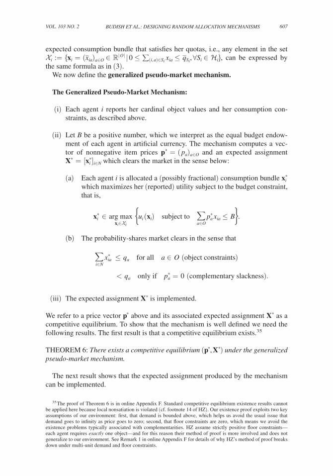
We now define the generalized pseudo-market mechanism.
The Generalized Pseudo-Market Mechanism:
(i) Each agent i reports her cardinal object values and her consumption con-straints, as described above.
(ii) Let B be a positive number, which we interpret as the equal budget endow-ment of each agent in artificial currency. The mechanism computes a vec-tor of nonnegative item prices p * = ( p a ) a∈O and an expected assignment X * = [ x i * ] i∈N which clears the market in the sense below:
(a) Each agent i is allocated a (possibly fractional) consumption bundle x i * which maximizes her (reported) utility subject to the budget constraint, that is,
x i * ∈ arg max x i ∈ i
{ u i ( x i ) subject to ∑ a∈O
p a * x ia ≤ B}.
(b) The probability-shares market clears in the sense that
∑ i∈N
x ia * ≤ q a for all a ∈ O (object constraints)
< q a only if p a * = 0 (complementary slackness).
(iii) The expected assignment X * is implemented.
We refer to a price vector p * above and its associated expected assignment X * as a competitive equilibrium. To show that the mechanism is well defined we need the following results. The first result is that a competitive equilibrium exists.35
THEOREM 6: There exists a competitive equilibrium ( p * , X * ) under the generalized pseudo-market mechanism.
The next result shows that the expected assignment produced by the mechanism can be implemented.
35 The proof of Theorem 6 is in online Appendix F. Standard competitive equilibrium existence results cannot be applied here because local nonsatiation is violated (cf. footnote 14 of HZ). Our existence proof exploits two key assumptions of our environment: first, that demand is bounded above, which helps us avoid the usual issue that demand goes to infinity as price goes to zero; second, that floor constraints are zero, which means we avoid the existence problems typically associated with complementarities. HZ assume strictly positive floor constraints—each agent requires exactly one object—and for this reason their method of proof is more involved and does not generalize to our environment. See Remark 1 in online Appendix F for details of why HZ’s method of proof breaks down under multi-unit demand and floor constraints.
608 THE AMERICAN ECONOMIC REVIEW ApRIl 2013
COROLLARY 3: The expected assignment X * produced by the generalized pseudo-market mechanism is implementable. Moreover, there exists a lottery over pure assignments implementing X * such that the expected utility of each agent i is u i ( x i * ).
PROOF: The agents’ constraints form one hierarchy, while the objects’ capacity con-
straints form a second hierarchy, hence the constraint structure is a bihierarchy. Since the expected assignment X * satisfies all of the constraints, it is implementable by Theorem 1.
A. Properties of the Generalized Pseudo-Market Mechanism
The original HZ mechanism is attractive for single-unit assignment because it is ex ante efficient and envy free. We show that these properties carry over to our more general environment.
For the ex ante efficiency result, we make one additional technical assumption, which is that each agent’s bliss point is unique. That is, for each agent i, there is a unique element of
__ i that maximizes (3) for student i.36
THEOREM 7: The expected assignment X * is ex ante Pareto efficient, and every realization of the lottery is ex post Pareto efficient.
PROOF: Suppose there exists an expected assignment ̃ X = [ ̃ x i ] i∈N that Pareto improves
upon X * . If u i ( ̃ x i ) > u i ( x i * ) then revealed preference implies that p * ⋅ ̃ x i > p * ⋅ x i * . Suppose u i ( ̃ x i ) = u i ( x i * ). We claim that p * ⋅ ̃ x i ≥ p * ⋅ x i * . Toward a contradiction, sup-pose that p * ⋅ ̃ x i < p * ⋅ x i * . Let x i denote i ’s bliss point. From our assumption that bliss points are unique it follows that u i ( x i ) > u i ( ̃ x i ) = u i ( x i * ). Since p * ⋅ ̃ x i < p * ⋅ x i * ≤ B there exists λ ∈ (0, 1) such that p * ⋅ (λ x i + (1 − λ) ̃ x i ) ≤ B. By concavity of u and uniqueness of the bliss point, u i (λ x i + (1 − λ) ̃ x i ) > u i ( ̃ x i ) = u i ( x i * ), which contradicts x i * being a utility maximizer for i in Step (2) of the generalized pseudo-market mechanism. Hence p * ⋅ ̃ x i ≥ p * ⋅ x i * .
From the above and from the assumption that ̃ X is a Pareto improvement on X * , we have established that p * ⋅ ̃ x i ≥ p * ⋅ x i * for all i with at least one strict. Thus ∑i p * ⋅ ̃ x i > ∑i p * ⋅ x i * . It then follows that there exists a ∈ O such that p a * > 0 and ∑i ̃ x ia > ∑i x ia * . But this contradicts the complementary slackness condition of the pseudo market defined earlier, which implies that ∑i x ia * = q a . We thus conclude that X * is (ex ante) Pareto efficient.
Ex ante efficiency immediately implies ex post efficiency; if some realization of a lottery were ex post inefficient, then by executing Pareto improvements for that realization we could generate an ex ante Pareto improvement.
36 This assumption is made for technical convenience. Remark 2 in online Appendix F illustrates why this assumption is necessary to obtain ex ante Pareto efficiency under our mechanism as defined above, and also illus-trates how our mechanism can be modified to obtain ex ante efficiency even in cases in which an agent’s bliss point is not unique.
609budish et al.: designing random allocation mechanismsVol. 103 no. 2
THEOREM 8: The expected assignment X * is ex ante envy free. That is, for any agents i ≠ j, u i ( x i * ) ≥ u i ( x j * ).
PROOF: The result follows immediately from the definition of the mechanism given that
all agents have the same budget.
Theorem 8 concerns ex ante fairness. The main result of Section V can be used to enhance ex post fairness in cases where agents’ bids take a simple additive-separa-ble form without additional constraints.
Aside from accommodating multi-unit demand, our generalization of the pseudo-market mechanism allows agents to express several kinds of constraints that may be useful for practice. To fix ideas we focus on constraints specific to the problem of course allocation.
• Scheduling Constraints: Scheduling constraints can often be expressed by means of a hierarchy. One example is students at Harvard Business School, who require ten courses per school year, of which five should be in each of the two semesters, and of which no more than one should meet at any given time. These constraints form a hierarchy because the semester constraint sets are dis-joint subsets of the school-year constraint set, and the time-slot constraint sets are disjoint subsets of the semester constraint sets.
• Curricular Constraints: Students often seek variety in their schedules due to diminishing returns. Our class of preferences can accommodate constraints of the form “at most two courses in Finance,” and it can also accommodate more elaborate constraints like “at most two courses in Finance, at most two courses in Marketing, and at most three courses in Finance or Marketing.”
As was seen above, such constraints can be incorporated into the individual hierarchies { 1i } i∈N . A limitation of our formulation, however, is that we may not be able to accommodate multiple kinds of these constraints simultaneously. While ruling out some practical applications, this restriction is necessitated by imple-mentability. For instance, if there is a Finance course and a Marketing course that meet at time slot 1 ( f 1 , m 1 ), and another Finance course and another Marketing course that meet at time slot 2 ( f 2 , m 2 ), then scheduling constraints on { f 1 , m 1 } and { f 2 , m 2 } and curricular constraints on { f 1 , f 2 } and { m 1 , m 2 } cannot coexist in the same hierarchy.37
B. Accommodating Nonlinear Preferences
So far, we have assumed that agents’ preferences are linear (additive) on a domain specified by certain constraints. Yet, certain nonlinear preferences seem quite
37 Budish (2011) proposes a multi-unit assignment mechanism that accommodates arbitrary ordinal preferences over schedules, but which is only approximately ex post efficient. It too is based on the idea of CEEI, but uses the framework to find an ex post sure assignment; by contrast, we use CEEI to find an “expected” assignment. Additional discussion on the tradeoffs between these two approaches can be found in Section 8.2 of the working paper version of Budish (2011).
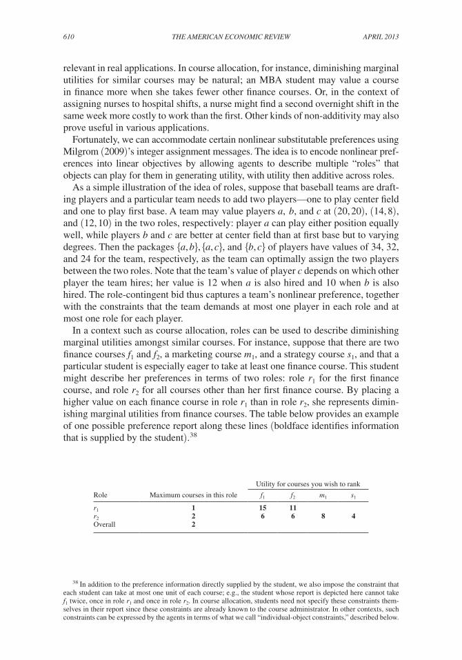
610 THE AMERICAN ECONOMIC REVIEW ApRIl 2013
relevant in real applications. In course allocation, for instance, diminishing marginal utilities for similar courses may be natural; an MBA student may value a course in finance more when she takes fewer other finance courses. Or, in the context of assigning nurses to hospital shifts, a nurse might find a second overnight shift in the same week more costly to work than the first. Other kinds of non-additivity may also prove useful in various applications.
Fortunately, we can accommodate certain nonlinear substitutable preferences using Milgrom (2009)’s integer assignment messages. The idea is to encode nonlinear pref-erences into linear objectives by allowing agents to describe multiple “roles” that objects can play for them in generating utility, with utility then additive across roles.
As a simple illustration of the idea of roles, suppose that baseball teams are draft-ing players and a particular team needs to add two players—one to play center field and one to play first base. A team may value players a, b, and c at (20, 20), (14, 8), and (12, 10) in the two roles, respectively: player a can play either position equally well, while players b and c are better at center field than at first base but to varying degrees. Then the packages {a, b}, {a, c}, and {b, c} of players have values of 34, 32, and 24 for the team, respectively, as the team can optimally assign the two players between the two roles. Note that the team’s value of player c depends on which other player the team hires; her value is 12 when a is also hired and 10 when b is also hired. The role-contingent bid thus captures a team’s nonlinear preference, together with the constraints that the team demands at most one player in each role and at most one role for each player.
In a context such as course allocation, roles can be used to describe diminishing marginal utilities amongst similar courses. For instance, suppose that there are two finance courses f1 and f2, a marketing course m1, and a strategy course s1, and that a particular student is especially eager to take at least one finance course. This student might describe her preferences in terms of two roles: role r1 for the first finance course, and role r2 for all courses other than her first finance course. By placing a higher value on each finance course in role r1 than in role r2, she represents dimin-ishing marginal utilities from finance courses. The table below provides an example of one possible preference report along these lines (boldface identifies information that is supplied by the student).38
38 In addition to the preference information directly supplied by the student, we also impose the constraint that each student can take at most one unit of each course; e.g., the student whose report is depicted here cannot take f1 twice, once in role r1 and once in role r2. In course allocation, students need not specify these constraints them-selves in their report since these constraints are already known to the course administrator. In other contexts, such constraints can be expressed by the agents in terms of what we call “individual-object constraints,” described below.
Utility for courses you wish to rank
Role Maximum courses in this role f1 f2 m1 s1
r1 1 15 11r2 2 6 6 8 4Overall 2
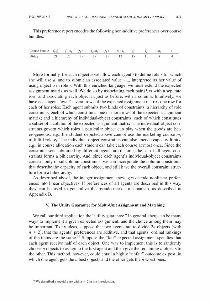
611budish et al.: designing random allocation mechanismsVol. 103 no. 2
This preference report encodes the following non-additive preferences over course bundles:
More formally, for each object a we allow each agent i to define role r for which she will use a, and to submit an associated value v ira , interpreted as her value of using object a in role r. With this enriched language, we must extend the expected assignment matrix as well. We do so by associating each pair (i, r) with a separate row, and associating each object a, just as before, with a column. Intuitively, we have each agent “own” several rows of the expected assignment matrix, one row for each of her roles. Each agent submits two kinds of constraints: a hierarchy of role constraints, each of which constitutes one or more rows of the expected assignment matrix; and a hierarchy of individual-object constraints, each of which constitutes a subset of a column of the expected assignment matrix. The individual-object con-straints govern which roles a particular object can play when the goods are het-erogeneous; e.g., the student depicted above cannot use the marketing course m 1 to fulfill role r 1 . The individual-object constraints can also encode capacity limits, e.g., in course allocation each student can take each course at most once. Since the constraint sets submitted by different agents are disjoint, the set of all agent con-straints forms a bihierarchy. And, since each agent’s individual-object constraints consists only of subcolumn constraints, we can incorporate the column constraints that describe the capacity of each object, and still have the overall constraint struc-ture form a bihierarchy.
As described above, the integer assignment messages encode nonlinear prefer-ences into linear objectives. If preferences of all agents are described in this way, they can be used to generalize the pseudo-market mechanism, as described in Appendix B.
V. The Utility Guarantee for Multi-Unit Assignment and Matching
We call our third application the “utility guarantee.” In general, there can be many ways to implement a given expected assignment, and the choice among them may be important. To fix ideas, suppose that two agents are to divide 2n objects (with n ≥ 2), that the agents’ preferences are additive, and that agents’ ordinal rankings of the items are the same.39 Suppose the “fair” expected assignment specifies that each agent receive half of each object. One way to implement this is to randomly choose n objects to assign to the first agent and then give the remaining n objects to the other. This method, however, could entail a highly “unfair” outcome ex post, in which one agent gets the n best objects and the other gets the n worst ones.
39 We described a special case with n = 2 in the introduction.
Course bundle f1, f2 f1, m1 f1, s1 f2, m1 f2, s1 m1, s1 f1 f2 m1 s1
Utility 21 23 19 19 15 12 15 11 8 4
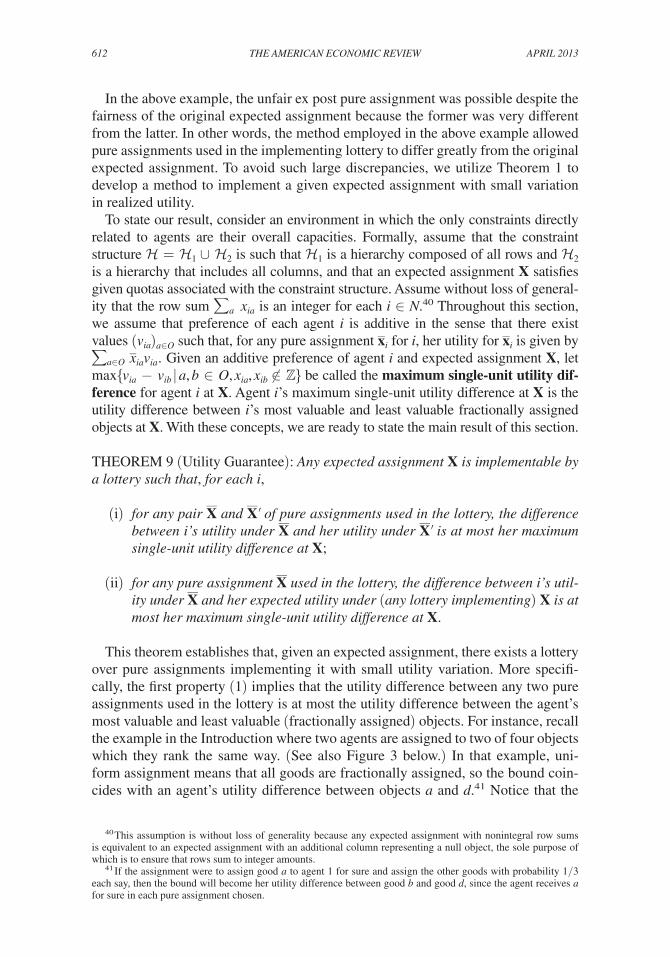
612 THE AMERICAN ECONOMIC REVIEW ApRIl 2013
In the above example, the unfair ex post pure assignment was possible despite the fairness of the original expected assignment because the former was very different from the latter. In other words, the method employed in the above example allowed pure assignments used in the implementing lottery to differ greatly from the original expected assignment. To avoid such large discrepancies, we utilize Theorem 1 to develop a method to implement a given expected assignment with small variation in realized utility.
To state our result, consider an environment in which the only constraints directly related to agents are their overall capacities. Formally, assume that the constraint structure = 1 ∪ 2 is such that 1 is a hierarchy composed of all rows and 2 is a hierarchy that includes all columns, and that an expected assignment X satisfies given quotas associated with the constraint structure. Assume without loss of general-ity that the row sum ∑ a
x ia is an integer for each i ∈ N.40 Throughout this section,
we assume that preference of each agent i is additive in the sense that there exist values ( v ia ) a∈O such that, for any pure assignment
_ x i for i, her utility for
_ x i is given by
∑ a∈O _ x ia v ia . Given an additive preference of agent i and expected assignment X, let
max{ v ia − v ib | a, b ∈ O, x ia , x ib ∉ 핑} be called the maximum single-unit utility dif-ference for agent i at X. Agent i ’s maximum single-unit utility difference at X is the utility difference between i ’s most valuable and least valuable fractionally assigned objects at X. With these concepts, we are ready to state the main result of this section.
THEOREM 9 (Utility Guarantee): Any expected assignment X is implementable by a lottery such that, for each i,
(i) for any pair __
X and __
X ′ of pure assignments used in the lottery, the difference between i’s utility under
__ X and her utility under
__ X ′ is at most her maximum
single-unit utility difference at X;
(ii) for any pure assignment __
X used in the lottery, the difference between i’s util-ity under
__ X and her expected utility under (any lottery implementing) X is at
most her maximum single-unit utility difference at X.
This theorem establishes that, given an expected assignment, there exists a lottery over pure assignments implementing it with small utility variation. More specifi-cally, the first property (1) implies that the utility difference between any two pure assignments used in the lottery is at most the utility difference between the agent’s most valuable and least valuable (fractionally assigned) objects. For instance, recall the example in the Introduction where two agents are assigned to two of four objects which they rank the same way. (See also Figure 3 below.) In that example, uni-form assignment means that all goods are fractionally assigned, so the bound coin-cides with an agent’s utility difference between objects a and d.41 Notice that the
40 This assumption is without loss of generality because any expected assignment with nonintegral row sums is equivalent to an expected assignment with an additional column representing a null object, the sole purpose of which is to ensure that rows sum to integer amounts.
41 If the assignment were to assign good a to agent 1 for sure and assign the other goods with probability 1/3 each say, then the bound will become her utility difference between good b and good d, since the agent receives a for sure in each pure assignment chosen.
613budish et al.: designing random allocation mechanismsVol. 103 no. 2
Theorem 9 bound is vacuous when agents have single-unit demand, and is most powerful when agents demand many goods each. The second property (2) is an immediate corollary of the first one, providing a bound on the difference between the expected utility of the given expected assignment and the utility of any pure assignment used in the lottery.
A proof sketch of Theorem 9 can be given based on Theorem 1. The idea is to supplement the actual constraints of the problem with a set of artificial “utility prox-imity” constraints as follows. For each agent i and integer k, the kth constraint set of agent i, S ik , consists of her 1st, 2nd, … , kth most preferred objects; its floor and ceiling constraints are ⌊ ∑a∈ S ik x ia ⌋ and ⌈ ∑a∈ S ik x ia ⌉ , respectively. The resulting con-straint structure is still a bihierarchy after this addition, so Theorem 1 guarantees that the expected assignment can be implemented with all of the constraints satis-fied. Satisfying the artificial “utility proximity” constraints means that in each real-ized assignment, each agent receives her k most preferred objects, for each k, with approximately the same probability as in the original expected assignment, thus resulting in small utility variation. To illustrate, recall the example in the Introduction where two agents are assigned to two of four objects which they rank the same way. The supplementary constraints are depicted in Figure 3, and entail the requirement: each agent must get one of a and b, at most two out of a, b, and c, and two objects in total.42 The utility difference between the best and worst implementation is then no more than the difference between one’s values of a (most preferred) and d (least preferred), as stated by Theorem 9.
Theorem 9 can be used to augment ex post fairness in conjunction with some multi-unit expected assignment algorithm. We say that an expected assignment X satisfies ex ante equal treatment of equals if, for any pair of agents i and j whose utility functions are identical, i and j are indifferent between x i and x j . The following claim is an immediate corollary of Theorem 9.
COROLLARY 4: Suppose that i and j have identical utility functions and a given expected assignment X satisfies ex ante equal treatment of equals. Then there exists a lottery implementing X such that, for any pure assignment used in the lottery, the difference between i’s utility under her pure assignment and her utility under j’s pure assignment is at most her maximum single-unit utility difference at X.
42 In the 2n object example at the beginning of this section, for instance, the above artificial constraints require that an agent receive either zero or one unit of her top object, exactly one from her top two objects, either one or two from her top three, exactly two from her top four, and so on.
0.5 0.5 0.5 0.5
0.5 0.5 0.5 0.5( )Figure 3. Illustration of the Utility Guarantee
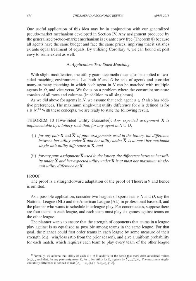
614 THE AMERICAN ECONOMIC REVIEW ApRIl 2013
One useful application of this idea may be in conjunction with our generalized pseudo-market mechanism developed in Section IV. Any assignment produced by the generalized pseudo-market mechanism is ex ante envy free (Theorem 8) because all agents have the same budget and face the same prices, implying that it satisfies ex ante equal treatment of equals. By utilizing Corollary 4, we can bound ex post envy to some extent as well.
A. Application: Two-Sided Matching
With slight modification, the utility guarantee method can also be applied to two-sided matching environments. Let both N and O be sets of agents and consider many-to-many matching in which each agent in N can be matched with multiple agents in O, and vice versa. We focus on a problem where the constraint structure consists of all rows and columns (in addition to all singletons).
As we did above for agents in N, we assume that each agent a ∈ O also has addi-tive preferences. The maximum single-unit utility difference for a is defined as for i ∈ N.43 With these concepts, we are ready to state the following result.
THEOREM 10 (Two-Sided Utility Guarantee): Any expected assignment X is implementable by a lottery such that, for any agent in N ∪ O,
(i) for any pair X and __
X ′ of pure assignments used in the lottery, the difference between her utility under
__ X and her utility under
__ X ′ is at most her maximum
single-unit utility difference at X, and
(ii) for any pure assignment __
X used in the lottery, the difference between her util-ity under
__ X and her expected utility under X is at most her maximum single-
unit utility difference at X.
PROOF: The proof is a straightforward adaptation of the proof of Theorem 9 and hence
is omitted.
As a possible application, consider two leagues of sports teams N and O, say the National League (NL) and the American League (AL) in professional baseball, and the planner who wants to schedule interleague play. For concreteness, suppose there are four teams in each league, and each team must play six games against teams on the other league.
The planner wants to ensure that the strength of opponents that teams in a league play against is as equalized as possible among teams in the same league. For that goal, the planner could first order teams in each league by some measure of their strength (e.g., win/loss ratio from the prior season), and give a uniform probability for each match, which requires each team to play every team of the other league
43 Formally, we assume that utility of each a ∈ O is additive in the sense that there exist associated values ( w ia ) i∈N such that, for any pure assignment
_ x a for a, her utility for
_ x a is given by ∑ i∈N
_ x ia w ia . The maximum single-
unit utility difference is defined as max{ w ia − w ja | i, j ∈ N, x ia , x ja ∉ 핑}.
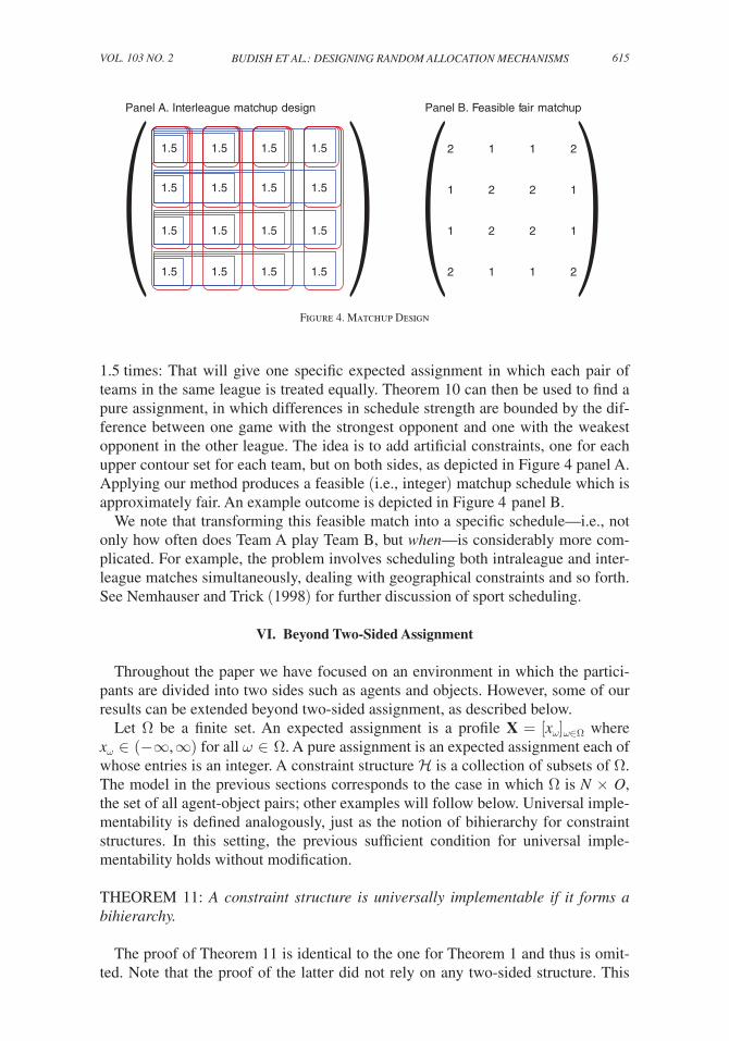
615budish et al.: designing random allocation mechanismsVol. 103 no. 2
1.5 times: That will give one specific expected assignment in which each pair of teams in the same league is treated equally. Theorem 10 can then be used to find a pure assignment, in which differences in schedule strength are bounded by the dif-ference between one game with the strongest opponent and one with the weakest opponent in the other league. The idea is to add artificial constraints, one for each upper contour set for each team, but on both sides, as depicted in Figure 4 panel A. Applying our method produces a feasible (i.e., integer) matchup schedule which is approximately fair. An example outcome is depicted in Figure 4 panel B.
We note that transforming this feasible match into a specific schedule—i.e., not only how often does Team A play Team B, but when—is considerably more com-plicated. For example, the problem involves scheduling both intraleague and inter-league matches simultaneously, dealing with geographical constraints and so forth. See Nemhauser and Trick (1998) for further discussion of sport scheduling.
VI. Beyond Two-Sided Assignment
Throughout the paper we have focused on an environment in which the partici-pants are divided into two sides such as agents and objects. However, some of our results can be extended beyond two-sided assignment, as described below.
Let Ω be a finite set. An expected assignment is a profile X = [ x ω ] ω∈Ω where x ω ∈ (− ∞, ∞) for all ω ∈ Ω. A pure assignment is an expected assignment each of whose entries is an integer. A constraint structure is a collection of subsets of Ω. The model in the previous sections corresponds to the case in which Ω is N × O, the set of all agent-object pairs; other examples will follow below. Universal imple-mentability is defined analogously, just as the notion of bihierarchy for constraint structures. In this setting, the previous sufficient condition for universal imple-mentability holds without modification.
THEOREM 11: A constraint structure is universally implementable if it forms a bihierarchy.
The proof of Theorem 11 is identical to the one for Theorem 1 and thus is omit-ted. Note that the proof of the latter did not rely on any two-sided structure. This
1.5 1.5 1.5 1.5
1.5 1.5 1.5 1.5
1.5 1.5 1.5 1.5
1.5 1.5 1.5 1.5
Panel A. Interleague matchup design
2 1 1 2
1 2 2 1
1 2 2 1
2 1 1 2
Panel B. Feasible fair matchup
( ) ( )Figure 4. Matchup Design
616 THE AMERICAN ECONOMIC REVIEW ApRIl 2013
observation raises a question about what situations beyond two-sided assignment are amenable to the expected assignment approach of HZ and BM. What about assign-ment problems in which there are more than two sides (“multi-sided assignment”) or no restriction on matching within a given side (“roommate matching”)? We shall see below that such structures do not generally admit universal implementability. To show this, however, it is not enough to show that they are not bihierarchical, for a bihierarchy is sufficient but not necessary for universal implementability.
We thus develop a necessary condition for universal implementability inspired by Example 1. In that example, a “cycle” formed by three constraint sets (the first row, the first column, and the diagonal set) leads to a situation where at least one of the constraints is violated. We will see that in fact a cycle of any “odd” number of inter-secting constraint sets can cause the same sort of situation. To argue this formally, we first define an odd cycle as follows:
DEFINITION 4: A sequence of l constraint sets ( S 1 , … , S l ) in is an odd cycle if
(i) l is odd;
(ii) there exists a sequence of agent-object pairs ( s 1 , … , s l ) such that, for each i = 1, … , l, we have
(a) s i ∈ S i ∩ S i+1 (subscript l + 1 should be interpreted as 1)
(b) s i ∉ S j for any j ≠ i, i + 1.
An argument generalizing Example 1 yields the following (a formal proof is in the online Appendix).
LEMMA 1 (Odd Cycles): If a constraint structure contains an odd cycle, then it is not universally implementable.
Remark 1: Theorem 11 and Lemma 1 together imply that a bihierarchical con-straint structure is universally implementable and that a universally implementable constrained structure cannot involve an odd cycle. We saw in footnote 19 that the converse of the first statement does not hold. It turns out that the converse of the second statement does not hold, either—namely, “no odd cycles” does not imply universal implementability. To see this, consider
= { {(1, a), (1, b)}, {(1, a), (2, a)}, {(1, a), (2, b)}, {(1, a), (1, b), (2, a), (2, b)} } .
This structure does not contain an odd cycle (and it is not a bihierarchy). Assume the quota for each of the first three sets is one and the quota for the last set is two. Now consider the expected assignment X of Example 1. Even though X satisfies the quotas, it is not implementable. Importantly, however, the “gaps” across these three conditions—bihierarchy, universal implementability, and no odd cycles—vanish in the canonical two-sided constraint structure. The proof of Theorem 2 shows that if a canonical two-sided constraint structure fails to be a bihierarchy, it must involve
617budish et al.: designing random allocation mechanismsVol. 103 no. 2
an odd cycle, thus implying that all three conditions coincide when the constraint structure is canonically two-sided.
We can apply Lemma 1 to show the difficulty one faces in implementing expected assignments in multi-sided assignment and roommate matching.
A. Multi-Sided Assignment
Thus far, we have focused on two-sided assignment environments in which agents on one side are assigned objects (or agents) on the other side. As noted before, many important market design problems fall into the two-sided assignment environment. Sometimes, however, matching involves more than two sides. For instance, students may be assigned to different schools and after-school programs, in which case the matching must be three-sided, consisting of student/school/after-school triples. Or, manufacturers may need to match with multiple suppliers, ensuring mutual compat-ibility of products or the right combination of capabilities.
Our main point is most easily made by starting with a three-sided matching prob-lem in which we introduce another finite set L of (say) agents, in addition to N and O. A matching then consists of a triple (i, a, l) ∈ N × O × L, and an expected assignment is defined by a profile X = [ x (i, a, l) ] (i, a, l)∈N×O×L that assigns a real num-ber to each triple (i, a, l). Constraints on the expected assignment can be described as before via the constraint structure, i.e., the sets of (i, a, l)’s whose entries are subject to ceiling or floor quota constraints. That is, the constraint structure ⊂ 2 N×O×L is a collection of subsets of N × O × L. As in the classical setup, the basic constraints arise from the fact that each agent in N, each object in O, and each agent in L are assigned to some pair in the other two sides (which may include a null object or a null agent). Hence, it is natural to assume that contains the sets {{i} × O × L | i ∈ N}, {N × {a} × L | a ∈ O}, and {N × O × {l} | l ∈ L}. We call such a constraint structure a canonical three-sided constraint structure.
Notice that the problem reduces to that of two-sided assignment if N or O or L is a singleton set, implying that a canonical three-sided constraint structure in such problems is universally implementable. It turns out that, except for such cases, no analogue of the Birkhoff-von Neumann theorem holds in three-sided matching.
THEOREM 12 (Impossibility with Three-Sided Assignment): No canonical three-sided constraint structure with | N |, | O |, | L | ≥ 2 is universally implementable.
PROOF: We prove the result by showing that any canonical three-sided constraint structure
with | N |, | O |, | L | ≥ 2 contains an odd cycle. By Lemma 1, this is sufficient for the failure of universal implementability (as pointed out before, even though the proof of Lemma 1 formally deals with the two-sided matching setup, its proof does not depend on it).
Fix i ∈ N, a ∈ O, l ∈ L and consider three sets S i := {i} × O × L, S a := N × {a} × L, and S l := N × O × {l}. Fix i′ ∈ N, a′ ∈ O, l′ ∈ L such that i′ ≠ i, a′ ≠ a, and l′ ≠ l (such i′, a′, and l′ exist since | N |, | O |, | L | ≥ 2). Then (i, a, l′ ) ∈ S i ∩ S a \ S l , (i, a′, l) ∈ S i ∩ S l \ S a , and (i′, a, l) ∈ S a ∩ S l \ S i . We thus conclude that S i , S a , and S l form an odd cycle.
618 THE AMERICAN ECONOMIC REVIEW ApRIl 2013
It is clear from the proof that the same impossibility result holds for any multi-sided matching of more than two kinds of agents.
Remark 2 (Matching with Contracts): Firms sometimes hire workers for differ-ent positions with different terms of contract. For instance, hospitals hire medical residents for different kinds of positions (such as research and clinical positions), and different positions may entail different duties and compensations. To encom-pass such situations, Hatfield and Milgrom (2005) develop a model of “matching with contracts,” in which a matching specifies not only which firm employs a given worker but also on what contract terms. At first glance, introducing contract terms may appear to transform the environment into a canonical three-sided matching setting. This is in fact not the case. If we let L denote the set of possible contract terms, there is no sense in which the constraint structure contains sets of the form N × O × {l}. In words, there is no reason that each contract term should be chosen by some worker-firm pair. Rather, matching with contracts can be subsumed into our two-sided assignment setup by redefining the object set as O′ := O × L.
B. Roommate Matching
The “roommate problem” describes another interesting matching problem, in which any agent can, in principle, be matched to any other. One example is “pair-wise kidney exchange” (Roth, Sönmez, and Ünver 2005), in which a kidney patient with a willing-but-incompatible donor is to be matched to another patient-donor pair. If two such pairs are successfully matched, then the donor in each pair donates her kidney to the patient of the other pair.
Formally, consider a (finite) set of agents, N with | N | ≥ 3. (If | N | < 3, then the problem is no different from two-sided matching.) Then, a set Ω := {{i, j} | i, j ∈ N } of possible (unordered) pairs of agents describes a possible roommate matching. If the pair {i, i} is formed, that means that i is unmatched. An expected assignment is a profile X = [ x ω ] ω∈Ω where x ω ∈ [0, 1] for all ω ∈ Ω and a constraint structure is a collec-tion of subsets of Ω. We assume that each i must be assigned to some agent (possibly herself), so must contain set S i := {{i, j} | j ∈ N } for each i ∈ N. We call a constraint structure satisfying this property a canonical roommate matching constraint structure.
Notice that the problem reduces to that of two-sided matching if there are two or fewer agents, implying that a canonical roommate matching constraint structure in such problems is universally implementable. The next result shows that these are the only cases for which universal implementability holds.
THEOREM 13 (Impossibility with Roommate Matching): No canonical roommate matching constraint structure with at least three agents is universally implementable.
PROOF: We prove the result by showing that any canonical roommate matching constraint
structure contains an odd cycle if there are at least three agents. Consider i, j, k ∈ N, who are all distinct (such agents exist since | N | ≥ 3). Then, {i, j} ∈ ( S i ∩ S j ) \ S k ,
619budish et al.: designing random allocation mechanismsVol. 103 no. 2
{ j, k} ∈ ( S j ∩ S k ) \ S i , and {i, k} ∈ ( S i ∩ S k ) \ S j . We thus conclude that S i , S j , and S k form an odd cycle.
VII. Conclusion
This paper extends the expected assignment method to an expanded class of problems, including many-to-one and many-to-many matching, and problems with certain auxiliary constraints. We apply our results to extend two prominent mechanisms—BM’s probabilistic serial mechanism and HZ’s pseudo-market mechanism—to accommodate features such as group-specific quotas, endogenous capacities, multi-unit and non-additive demand, and scheduling constraints. We also develop a “utility guarantee” method which can be used to supplement the ex ante fairness promoted by randomization, by limiting the extent of ex post unfairness.
Methodologically, the paper identifies a maximal generalization of the Birkhoff-von Neumann theorem, demonstrating that the bihierarchy condition is both necessary and sufficient for a constraint structure to be universally implementable in canonical two-sided environments. We find that there is no similar universal implementability property for matching with three sides or more, nor for roommate problems.
The central goal of research in market design is to facilitate applications, and we hope that the tools and mechanisms described herein herald still further applications to come.
Appendix A Definition of the Generalized Probabilistic Serial Mechanism
Formally, the generalized probabilistic serial mechanism is defined through the fol-lowing symmetric simultaneous eating algorithm, or the eating algorithm for short.
Generalized Probabilistic Serial Mechanism. For any (i, a) ∈ S⊆N × O, let
χ (i, a, S) = 1 if (i, a) ∈ S and a ⪰ i b for any b with (i, b) ∈ S, { 0 otherwise,
be the indicator function that a is the most preferred object for i among objects b such that (i, b) is listed in S.
Given a preference profile ≻, the eating algorithm is defined by the following sequence of steps. Let S 0 = N × O, t 0 = 0, and x ia 0
= 0 for every i ∈ N and a ∈ O. Given S 0 , t 0 , X 0 = [ x ia 0
] i∈N, a∈O , … , S v−1 , t v−1 , X v−1 = [ x ia v−1 ] i∈N, a∈O , for any (i, a) ∈ S v−1 define
(A1) t v (i, a) = min S∈ 2 :(i, a)∈S
sup { t ∈ [0, 1] | ∑ ( j, b)∈S
[ x jb v−1 + χ ( j, b, S v−1 )(t − t v−1 )] < _ q S } ,(A2) t v = min
(i, a)∈ S v−1 t v (i, a),
(A3) S v = S v−1 \ {(i, a) ∈ S v−1 | t v (i, a) = t v },
620 THE AMERICAN ECONOMIC REVIEW ApRIl 2013
(A4) x ia v = x ia v−1 + χ (i, a, S v−1 )( t v − t v−1 ).
Since N × O is a finite set, there exists _ v such that t
_ v = 1. We define PS(≻) := X
_ v
to be the generalized probabilistic serial expected assignment for the preference profile ≻.
Appendix B Extended Framework for the Pseudo-Market Mechanism
Here, we discuss how the basic framework of Section IV can be extended to accommodate more general preferences, following Milgrom’s (2009) class of inte-ger assignment messages. As before, each agent i ∈ N submits cardinal values and a set of constraints. The main difference versus before is that the cardinal utility value associated with a particular object may vary depending on the “role” that object plays for the agent. Specifically, agent i reports the set of roles that are relevant for her, R i , cardinal utilities v ira for each r, a that describe the value for her of object a in role r, and a set of constraints that satisfy the following requirements. First, the agent may submit a hierarchical set of constraints ir for each role r, with each ir containing the “row” constraint (i, r) × A; we call these “single-role constraints,” and associate each agent-role pair (i, r) with its own row of an expected assignment matrix. Second, the agent submits a hierarchical set i0 of constraints pertaining to i ’s total quantity across multiple roles; each of these sets contains multiple rows (“multi-role constraints”). Last, for each object a ∈ O the agent submits a hierarchi-cal set of constraints pertaining to i ’s consumption of object a across her multiple rows; each of these sets corresponds to a subset of the column for object a (“object-specific constraints”). In course allocation, for instance, these object-specific con-straints ensure that each student gets at most one seat in any course, even if a course appears in multiple rows. Let i denote the union of all of i ’s constraints.
As described in the main text, each agent’s valuations and constraints together define her utility on an extended space of consumption bundles used in particular roles. This formulation induces the agent’s utility function over consumption bun-dles in a natural manner, as follows. Let integer-valued vector
_ x i = ( _ x ia ) a∈O denote a
consumption bundle for agent i. The utility for i from consumption bundle _ x i is the
solution to the following integer program:
u i ( _ x i ) = max ∑
r∈ R i
∑ a∈O
v ira _ x ira subject to
( ∑ r∈ R i
_ x ira ) a∈O
= _ x i (adding up constraint)
0 ≤ ∑ {((i, r), a)}∈ S i
_ x ira ≤ _ q S i for all S i ∈ i (agent constraints)
_ x ira ∈ 핑 for all r, a.
621budish et al.: designing random allocation mechanismsVol. 103 no. 2
As with the initial model, this utility function can be extended to a fractional assignment x i ∈ 핉 | O | , so we can write u i ( x i ) for the agent’s utility from fractional bundle x i .
Given the assignment messages and utility functions defined this way, they can be used in a generalized pseudo-market mechanism as follows. Step 1 is to identify a competitive equilibrium outcome X * = [ x ia * ] of the pseudo-market, given these preferences and the specified incomes. Given the assignment x i * for each i, step 2 is to identify the assignment of those objects to roles that maximizes the agent’s total value, subject to the constraints associated with the roles; that is, to find a vector ( x ira * ) r∈ R i , a∈O which solves the above linear programming problem with respect to x i * . Step 3 is to compile the results of the preceding step into an expanded expected assignment matrix. In this matrix, rows correspond to agent-role pairs and columns correspond to objects. This matrix is to be resolved into a lottery over pure matrices, each of which satisfies the role constraints (row constraints), overall object con-straints for each agent (defined on a collection of rows), object constraints (column constraints), and singleton constraints. Since the constraints form a bihierarchy, Theorem 1 applies, and the equilibrium assignment can be implemented as a lottery over pure assignments that satisfy all the constraints.
To see that the existence of a competitive equilibrium extends to this setting, note first that the demand correspondence resulting from such a utility function can readily be shown to be nonempty, convex-valued and upper-hemicontinuous. Additionally, as described in the main text, the constraint structure consisting of the union of individual agents’ constraints as well as the object capacity constraints forms a bihierarchy. Given these properties, the generalized pseudo market mecha-nism can be constructed precisely as in the baseline case in the main text, and all subsequent results follow without modification of proofs.
REFERENCES
Abdulkadiro ̆ g lu, Atila. 2005. “College Admission with Affirmative Action.” International Journal of Game Theory 33 (4): 535–49.
Abdulkadiro ̆ g lu, Atila, Parag A. Pathak, and Alvin E. Roth. 2005. “The New York City High School Match.” American Economic Review 95 (2): 364–67.
Abdulkadiro ̆ g lu, Atila, Parag A. Pathak, and Alvin E. Roth. 2009. “Strategy-Proofness versus Effi-ciency in Matching with Indifferences: Redesigning the NYC High School Match.” American Eco-nomic Review 99 (5): 1954–78.
Abdulkadiro ̆ g lu, Atila, and Tayfun Sönmez. 1998. “Random Serial Dictatorship and the Core from Random Endowments in House Allocation Problems.” Econometrica 66 (3): 689–701.
Abdulkadiro ̆ g lu, Atila, and Tayfun Sönmez. 2003a. “Ordinal Efficiency and Dominated Sets of Assign-ments.” Journal of Economic Theory 112 (1): 157–72.
Abdulkadiro ̆ g lu, Atila, and Tayfun Sönmez. 2003b. “School Choice: A Mechanism Design Approach.” American Economic Review 93 (3): 729–47.
Baccara, Mariagiovanna, Ayse Imrohoroglu, Alistair J. Wilson, and Leeat Yariv. 2012. “A Field Study on Matching with Network Externalities.” American Economic Review 102 (5): 1773–804.
Birkhoff, Garrett. 1946. “Three Observations on Linear Algebra.” Univ. Nac. Tucumán, Revista A 5: 147–51.
Bogomolnaia, Anna, and Hervé Moulin. 2001. “A New Solution to the Random Assignment Problem.” Journal of Economic Theory 100 (2): 295–328.
Bogomolnaia, Anna, and Hervé Moulin. 2002. “A Simple Random Assignment Problem with a Unique Solution.” Economic Theory 19 (3): 623–35.
Budish, Eric. 2011. “The Combinatorial Assignment Problem: Approximate Competitive Equilibrium from Equal Incomes.” Journal of Political Economy 119 (6): 1061–103.
622 THE AMERICAN ECONOMIC REVIEW ApRIl 2013
Budish, Eric, and Estelle Cantillon. 2012. “The Multi-unit Assignment Problem: Theory and Evidence from Course Allocation at Harvard.” American Economic Review 102 (5): 2237–71.
Che, Yeon-Koo, Ian Gale, and Jinwoo Kim. Forthcoming. “Assigning Resources to Budget-Constrained Agents.” Review of Economic Studies.
Che, Yeon-Koo, and Fuhito Kojima. 2010. “Asymptotic Equivalence of Probabilistic Serial and Ran-dom Priority Mechanisms.” Econometrica 78 (5): 1625–72.
Chen, Yan, and Tayfun Sönmez. 2002. “Improving Efficiency of On-Campus Housing: An Experimen-tal Study.” American Economic Review 92 (5): 1669–86.
Crès, Hervé, and Hervé Moulin. 2001. “Scheduling with Opting Out: Improving upon Random Prior-ity.” Operations Research 49 (4): 565–77.
Edmonds, Jack. 1970. “Submodular Functions, Matroids, and Certain Polyhedra.” In Combinatorial Structures and Their Applications, edited by Richard Guy, Haim Hanani, Norbert Sauer, and Jona-than Schonheim, 69–87. New York: Gordon and Breach.
Ehlers, Lars, Isa Emin Hafalir, M. Bumin Yenmez, and Muhammed Ali Yildirim. 2011. “School Choice with Controlled Choice Constraints: Hard Bounds versus Soft Bounds.” Unpublished.
Ehlers, Lars, and Bettina Klaus. 2003. “Coalitional Strategy-Proof and Resource-Monotonic Solutions for Multiple Assignment Problems.” Social Choice and Welfare 21 (2): 265–80.
Gale, David, and Lloyd S. Shapley. 1962. “College Admissions and the Stability of Marriage.” Ameri-can Mathematical Monthly 69 (1): 9–15.
Hafalir, Isa Emin, M. Bumin Yenmez, and Muhammed Ali Yildirim. Forthcoming. “Effective Affirma-tive Action in School Choice.” Theoretical Economics.
Hatfield, John William. 2009. “Strategy-Proof, Efficient, and Nonbossy Quota Allocations.” Social Choice and Welfare 33 (3): 505–15.
Hatfield, John William, and Paul R. Milgrom. 2005. “Matching with Contracts.” American Economic Review 95 (4): 913–35.
Hoffman, Alan J., and Joseph B. Kruskal. 1956. “Integral Boundary Points of Convex Polyhedra.” In Linear Inequalities and Related Systems. Vol. 38. Annals of Mathematics Studies. Edited by H. Kuhn and A. Tucker, 223– 46. Princeton: Princeton University Press.
Hylland, Aanund, and Richard Zeckhauser. 1979. “The Efficient Allocation of Individuals to Posi-tions.” Journal of Political Economy 87 (2): 293–314.
Katta, Akshay-Kumar, and Jay Sethuraman. 2006. “A Solution to the Random Assignment Problem on the Full Preference Domain.” Journal of Economic Theory 131 (1): 231–50.
Kesten, Onur. 2009. “Why Do Popular Mechanisms Lack Efficiency in Random Environments?” Jour-nal of Economic Theory 144 (5): 2209–26.
Kojima, Fuhito. 2012. “School Choice: Impossibilities for Affirmative Action.” Games and Economic Behavior 75 (2): 685–93.
Kojima, Fuhito. 2009. “Random Assignment of Multiple Indivisible Objects.” Mathematical Social Sciences 57 (1): 134–42.
Kojima, Fuhito, and Mihai Manea. 2010. “Incentives in the Probabilistic Serial Mechanism.” Journal of Economic Theory 145 (1): 106–23.
Manea, Mihai. 2008. “A Constructive Proof of the Ordinal Efficiency Welfare Theorem.” Journal of Economic Theory 141 (1): 276–81.
Manea, Mihai. 2009. “Asymptotic Ordinal Inefficiency of Random Serial Dictatorship.” Theoretical Economics 4 (2): 165–97.
McLennan, Andrew. 2002. “Ordinal Efficiency and the Polyhedral Separating Hyperplane Theorem.” Journal of Economic Theory 105 (2): 435–49.
Milgrom, Paul. 2009. “Assignment Messages and Exchanges.” American Economic Journal: Micro-economics 1 (2): 95–113.
Nemhauser, George, and Michael Trick. 1998. “Scheduling a Major College Basketball Conference.” Operations Research 46 (1): 1–8.
Papai, Szilvia. 2001. “Strategyproof and Nonbossy Multiple Assignments.” Journal of Public Eco-nomic Theory 3 (3): 257–71.
Pathak, Parag A., and Jay Sethuraman. 2011. “Lotteries in Student Assignment: An Equivalence Result.” Theoretical Economics 6 (1): 1–17.
Pratt, John W., and Richard J. Zeckhauser. 1990. “The Fair and Efficient Division of the Winsor Fam-ily Silver.” Management Science 36 (11): 1293–1301.
Roth, Alvin E. 2007. “Repugnance as a Constraint on Markets.” Journal of Economic Perspectives 21 (3): 37–58.
Roth, Alvin E., Tayfun Sönmez, and M. Utku Ünver. 2005. “Pairwise Kidney Exchange.” Journal of Economic Theory 125 (2): 151–88.
623budish et al.: designing random allocation mechanismsVol. 103 no. 2
Shapley, Lloyd, and Herbert Scarf. 1974. “On Cores and Indivisibility.” Journal of Mathematical Eco-nomics 1 (1): 22–37.
Sönmez, Tayfun, and M. Utku Ünver. 2010. “Course Bidding at Business Schools.” International Eco-nomic Review 51 (1): 99–123.
von Neumann, John. 1953. “A Certain Zero-Sum Two-Person Game Equivalent to the Optimal Assign-ment Problem.” In Contributions to the Theory of Games. Vol. 2, edited by W. Kuhn and A.W. Tucker. Princeton: Princeton University Press, 1997.
Yilmaz, Ozgur. 2009. “Random Assignment under Weak Preferences.” Games and Economic Behav-ior 66 (1): 546–58.