Embed Size (px)
Citation preview

Intro. GANs Interpolation
Some New Insights on Regularization and InterpolationMotivated from Neural Networks
Tengyuan Liang
Econometrics and Statistics
1 / 60
Intro. GANs Interpolation
OUTLINE
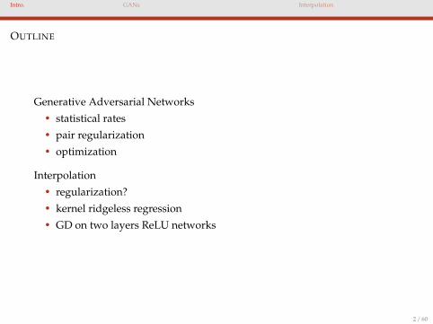
Generative Adversarial Networks• statistical rates• pair regularization• optimization
Interpolation• regularization?• kernel ridgeless regression• GD on two layers ReLU networks
2 / 60
Intro. GANs Interpolation
OUTLINE
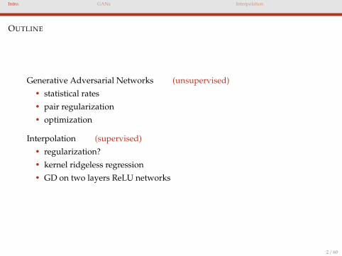
Generative Adversarial Networks (unsupervised)• statistical rates• pair regularization• optimization
Interpolation (supervised)• regularization?• kernel ridgeless regression• GD on two layers ReLU networks
2 / 60

Intro. GANs Interpolation
GANs
3 / 60
Intro. GANs Interpolation
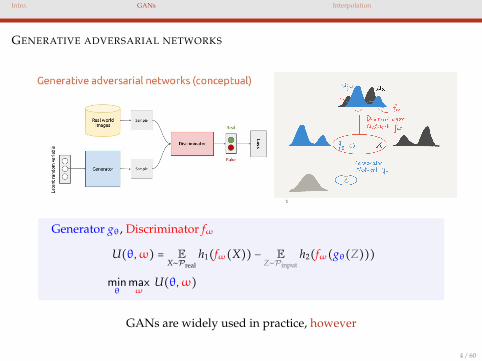
GENERATIVE ADVERSARIAL NETWORKS
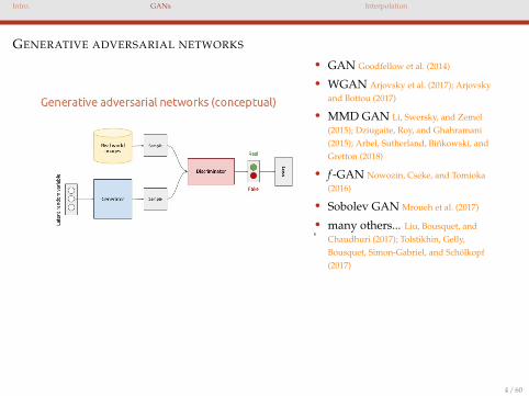
• GAN Goodfellow et al. (2014)
• WGAN Arjovsky et al. (2017); Arjovskyand Bottou (2017)
• MMD GAN Li, Swersky, and Zemel(2015); Dziugaite, Roy, and Ghahramani(2015); Arbel, Sutherland, Binkowski, andGretton (2018)
• f -GAN Nowozin, Cseke, and Tomioka(2016)
• Sobolev GAN Mroueh et al. (2017)
• many others... Liu, Bousquet, andChaudhuri (2017); Tolstikhin, Gelly,Bousquet, Simon-Gabriel, and Scholkopf(2017)
Generator gθ, Discriminator fω
U(θ,ω) = EX∼Preal
h1(fω(X)) − EZ∼Pinput
h2(fω(gθ(Z)))
minθ
maxω
U(θ,ω)
GANs are widely used in practice, however
4 / 60
Intro. GANs Interpolation
GENERATIVE ADVERSARIAL NETWORKS
Generator gθ, Discriminator fω
U(θ,ω) = EX∼Preal
h1(fω(X)) − EZ∼Pinput
h2(fω(gθ(Z)))
minθ
maxω
U(θ,ω)
GANs are widely used in practice, however
4 / 60
Intro. GANs Interpolation
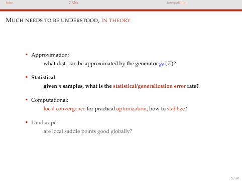
MUCH NEEDS TO BE UNDERSTOOD, IN THEORY
• Approximation:
what dist. can be approximated by the generator gθ(Z)?
• Statistical:
given n samples, what is the statistical/generalization error rate?
• Computational:
local convergence for practical optimization, how to stablize?
• Landscape:
are local saddle points good globally?
5 / 60
Intro. GANs Interpolation
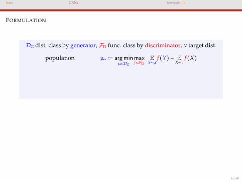
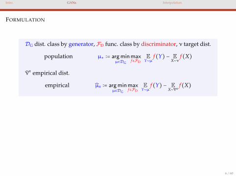
FORMULATION
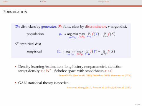
DG dist. class by generator, FD func. class by discriminator, ν target dist.
population µ∗ ∶= argminµ∈DG
maxf∈FD
EY∼µ
f(Y) − EX∼ν
f(X)
νn empirical dist.
empirical µn ∶= argminµ∈DG
maxf∈FD
EY∼µ
f(Y) − EX∼νn
f(X)
• Density learning/estimation: long history nonparametric statisticstarget density ν ∈ Wα - Sobolev space with smoothness α ≥ 0
Stone (1982); Nemirovski (2000); Tsybakov (2009); Wassermann (2006)
• GAN statistical theory is neededArora and Zhang (2017); Arora et al. (2017a,b); Liu et al. (2017)
6 / 60
Intro. GANs Interpolation
FORMULATION
DG dist. class by generator, FD func. class by discriminator, ν target dist.
population µ∗ ∶= argminµ∈DG
maxf∈FD
EY∼µ
f(Y) − EX∼ν
f(X)
νn empirical dist.
empirical µn ∶= argminµ∈DG
maxf∈FD
EY∼µ
f(Y) − EX∼νn
f(X)
• Density learning/estimation: long history nonparametric statisticstarget density ν ∈ Wα - Sobolev space with smoothness α ≥ 0
Stone (1982); Nemirovski (2000); Tsybakov (2009); Wassermann (2006)
• GAN statistical theory is neededArora and Zhang (2017); Arora et al. (2017a,b); Liu et al. (2017)
6 / 60
Intro. GANs Interpolation
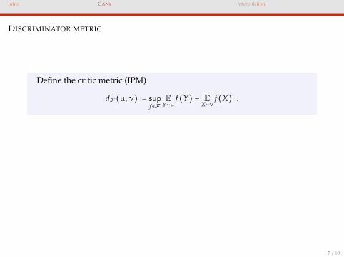
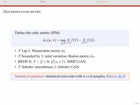
DISCRIMINATOR METRIC
Define the critic metric (IPM)
dF(µ,ν) ∶= supf∈F
EY∼µ
f(Y) − EX∼ν
f(X) .
• F Lip-1: Wasserstein metric dW
• F bounded by 1: total variation/Radon metric dTV
• RKHSH, F = f ∈H, ∥f∥H ≤ 1: MMD GAN• F Sobolev smoothness β: Sobolev GAN
Statistical question: statistical error rate with n-i.i.d samples, E dF(ν, µn)?
7 / 60
Intro. GANs Interpolation
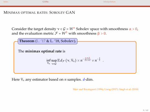
MINIMAX OPTIMAL RATES: SOBOLEV GAN
Consider the target density ν ∈ G = Wα Sobolev space with smoothness α > 0,and the evaluation metric F = Wβ with smoothness β > 0.
The minimax optimal rate is
infνn
supν∈G
E dF (ν, νn) ≍ n−α+β2α+d ∨ n−
12 .
Theorem (L. ’17 & L. ’18, Sobolev).
Here νn any estimator based on n samples. d-dim.
Mair and Ruymgaart (1996); Liang (2017); Singh et al. (2018)
8 / 60
Intro. GANs Interpolation
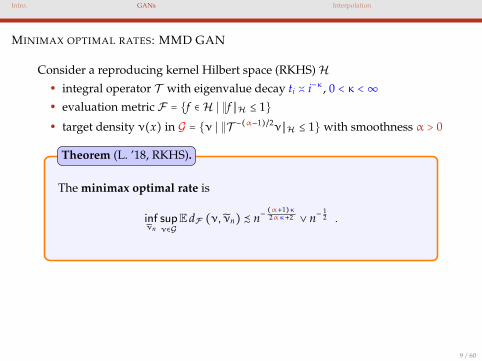
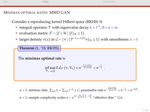
MINIMAX OPTIMAL RATES: MMD GAN
Consider a reproducing kernel Hilbert space (RKHS)H• integral operator T with eigenvalue decay ti ≍ i−κ, 0 < κ <∞• evaluation metric F = f ∈H ∣ ∥f∥H ≤ 1
• target density ν(x) in G = ν ∣ ∥T−(α−1)/2ν∥H ≤ 1 with smoothness α > 0
The minimax optimal rate is
infνn
supν∈G
E dF (ν, νn) ≾ n−(α+1)κ2ακ+2 ∨ n−
12 .
Theorem (L. ’18, RKHS).
κ > 1: intrinsic dim. ∑i≥1 ti = ∑i≥1 i−κ ≤ C, parametric rate n−(α+1)κ2ακ+2 ∨ n−
12 = n−1/2.
κ < 1: sample complexity scales n = ε2+ 2α+1 (
1κ−1), “effective dim.” 1/κ.
9 / 60
Intro. GANs Interpolation
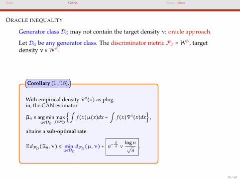
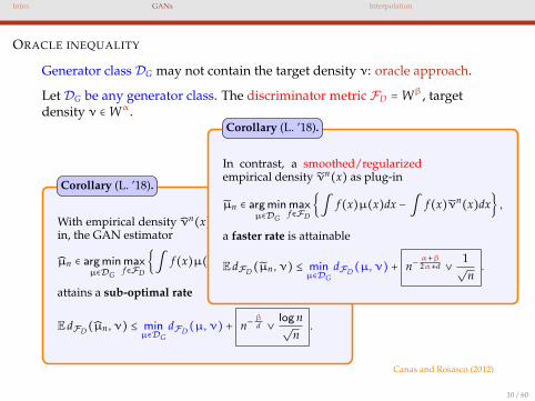
ORACLE INEQUALITY
Generator class DG may not contain the target density ν: oracle approach.
Let DG be any generator class. The discriminator metric FD = Wβ, targetdensity ν ∈ Wα.
With empirical density νn(x) as plug-in, the GAN estimator
µn ∈ argminµ∈DG
maxf∈FD
∫ f(x)µ(x)dx − ∫ f(x)νn(x)dx ,
attains a sub-optimal rate
E dFD(µn,ν) ≤ minµ∈DG
dFD(µ,ν) + n−βd ∨
log n√
n.
Corollary (L. ’18).
In contrast, a smoothed/regularizedempirical density νn(x) as plug-in
µn ∈ argminµ∈DG
maxf∈FD
∫ f(x)µ(x)dx − ∫ f(x)νn(x)dx ,
a faster rate is attainable
E dFD(µn,ν) ≤ minµ∈DG
dFD(µ,ν) + n−α+β2α+d ∨
1√
n.
Corollary (L. ’18).
Canas and Rosasco (2012)
10 / 60
Intro. GANs Interpolation
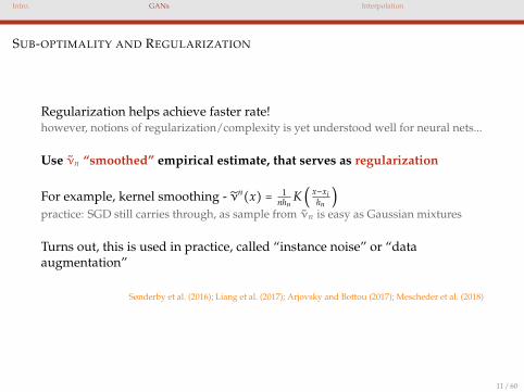
SUB-OPTIMALITY AND REGULARIZATION
Regularization helps achieve faster rate!however, notions of regularization/complexity is yet understood well for neural nets...
Use νn “smoothed” empirical estimate, that serves as regularization
For example, kernel smoothing - νn(x) = 1
nhnK (
x−xihn
)
practice: SGD still carries through, as sample from νn is easy as Gaussian mixtures
Turns out, this is used in practice, called “instance noise” or “dataaugmentation”
Sønderby et al. (2016); Liang et al. (2017); Arjovsky and Bottou (2017); Mescheder et al. (2018)
11 / 60

Intro. GANs Interpolation
Parametric results and pair regularization
12 / 60
Intro. GANs Interpolation
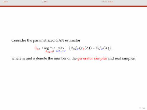
Consider the parametrized GAN estimator
θm,n ∈ argminθ∶gθ∈G
maxω∶fω∈F
Emfω(gθ(Z)) − Enfω(X) ,
where m and n denote the number of the generator samples and real samples.
13 / 60
Intro. GANs Interpolation
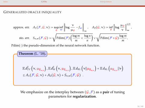
GENERALIZED ORACLE INEQUALITY
approx. err. A1(F ,G,ν) ∶= supθ
infω
∥logν
µθ− fω∥
∞, A2(G,ν) ∶= inf
θ∥log
µθ
ν∥
1/2
∞,
sto. err. Sn,m(F ,G) ∶=
√
Pdim(F) (logm
m∨log n
n) ∨
√
Pdim(F G)logm
m,
Pdim(⋅) the pseudo-dimension of the neural network function.
E d2TV (ν,µθm,n
) ,E d2W (ν,µθm,n
) ,E dKL (ν∣∣µθm,n) + E dKL (µθm,n
∣∣ν)
≤ A1(F ,G,ν) +A2(G,ν) + Sn,m(F ,G) .
Theorem (L. ’18).
We emphasize on the interplay between (G,F) as a pair of tuningparameters for regularization.
14 / 60
Intro. GANs Interpolation
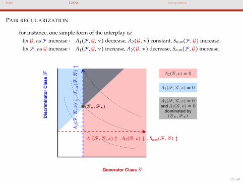
PAIR REGULARIZATION
for instance, one simple form of the interplay is:fix G, as F increase ∶ A1(F ,G,ν) decrease, A2(G,ν) constant, Sn,m(F ,G) increase,fix F , as G increase ∶ A1(F ,G,ν) increase, A2(G,ν) decrease, Sn,m(F ,G) increase.
Generator Class
Dis
crim
inat
or C
lass
and
dominated by
, ,
,
15 / 60

Intro. GANs Interpolation
Applications of pair regularization
16 / 60
Intro. GANs Interpolation
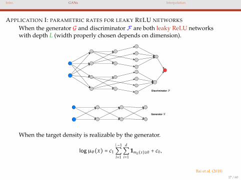
APPLICATION I: PARAMETRIC RATES FOR LEAKY RELU NETWORKS
When the generator G and discriminator F are both leaky ReLU networkswith depth L (width properly chosen depends on dimension).
Generator
Discriminator
When the target density is realizable by the generator.
logµθ(x) = c1
L−1
∑l=1
d
∑i=1
1mli(x)≥0 + c0,
Bai et al. (2018)17 / 60
Intro. GANs Interpolation
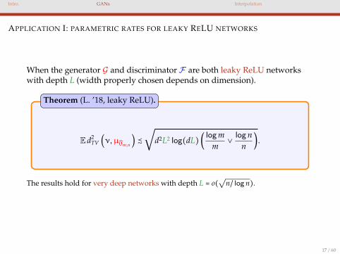
APPLICATION I: PARAMETRIC RATES FOR LEAKY RELU NETWORKS
When the generator G and discriminator F are both leaky ReLU networkswith depth L (width properly chosen depends on dimension).
E d2TV (ν,µθm,n
) ≾
√
d2L2 log(dL) (logm
m∨logn
n).
Theorem (L. ’18, leaky ReLU).
The results hold for very deep networks with depth L = o(√
n/ log n).
17 / 60
Intro. GANs Interpolation
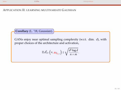
APPLICATION II: LEARNING MULTIVARIATE GAUSSIAN
GANs enjoy near optimal sampling complexity (w.r.t. dim. d), withproper choices of the architecture and activation,
E d2TV (ν,µθm,n
) ≾
√d2 log dn ∧m
.
Corollary (L. ’18, Gaussian).
18 / 60
Intro. GANs Interpolation
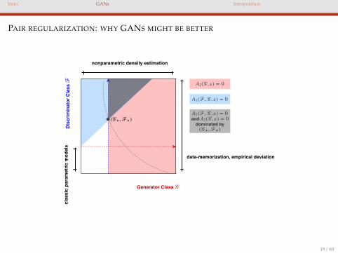
PAIR REGULARIZATION: WHY GANS MIGHT BE BETTER
Generator Class
Dis
crim
inat
or C
lass
and
dominated by
data-memorization, empirical deviation
nonparametric density estimation cl
assi
c pa
ram
etric
mod
els
19 / 60

Intro. GANs Interpolation
Optimization: local convergence
20 / 60
Intro. GANs Interpolation
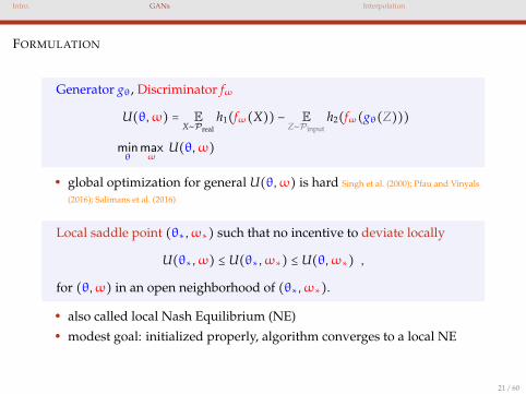
FORMULATION
Generator gθ, Discriminator fω
U(θ,ω) = EX∼Preal
h1(fω(X)) − EZ∼Pinput
h2(fω(gθ(Z)))
minθ
maxω
U(θ,ω)
• global optimization for general U(θ,ω) is hard Singh et al. (2000); Pfau and Vinyals
(2016); Salimans et al. (2016)
Local saddle point (θ∗,ω∗) such that no incentive to deviate locally
U(θ∗,ω) ≤ U(θ∗,ω∗) ≤ U(θ,ω∗) ,
for (θ,ω) in an open neighborhood of (θ∗,ω∗).
• also called local Nash Equilibrium (NE)• modest goal: initialized properly, algorithm converges to a local NE
21 / 60
Intro. GANs Interpolation
MAIN MESSAGE: INTERACTION MATTERS
Exponential local convergence to stable equilibrium
However, “interaction term” matters, slows down the convergence⇐ curse
What if unstable? turns out “interaction term” matters, utilize it rendersexponential convergence⇐ blessing
22 / 60
Intro. GANs Interpolation
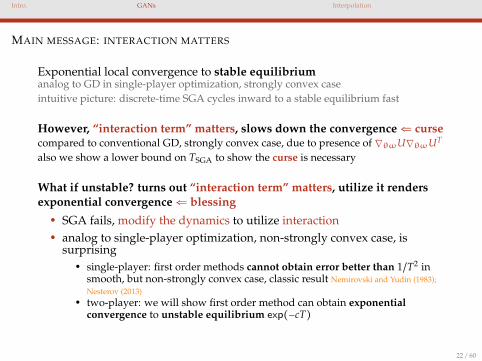
MAIN MESSAGE: INTERACTION MATTERS
Exponential local convergence to stable equilibriumanalog to GD in single-player optimization, strongly convex caseintuitive picture: discrete-time SGA cycles inward to a stable equilibrium fast
However, “interaction term” matters, slows down the convergence⇐ cursecompared to conventional GD, strongly convex case, due to presence of ∇θωU∇θωUT
also we show a lower bound on TSGA to show the curse is necessary
What if unstable? turns out “interaction term” matters, utilize it rendersexponential convergence⇐ blessing
• SGA fails, modify the dynamics to utilize interaction• analog to single-player optimization, non-strongly convex case, is
surprising• single-player: first order methods cannot obtain error better than 1/T2 in
smooth, but non-strongly convex case, classic result Nemirovski and Yudin (1983);Nesterov (2013)
• two-player: we will show first order method can obtain exponentialconvergence to unstable equilibrium exp(−cT)
22 / 60

Intro. GANs Interpolation
“However, no guarantees are known beyond the convex-concave setting and, moreimportantly for the paper, even in convex-concave games, no guarantees are knownfor the last-iterate pair.”
— Daskalakis, Ilyas, Syrgkanis, and Zeng (2017)
23 / 60
Intro. GANs Interpolation
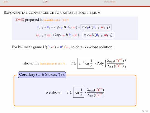
EXPONENTIAL CONVERGENCE TO UNSTABLE EQUILIBRIUM
OMD proposed in Daskalakis et al. (2017)
θt+1 = θt − 2η∇θU(θt,ωt) + η∇θU(θt−1,ωt−1)
ωt+1 =ωt + 2η∇ωU(θt,ωt) − η∇ωU(θt−1,ωt−1)
For bi-linear game U(θ,ω) = θTCω, to obtain ε-close solution
shown in Daskalakis et al. (2017) ∶ T ≿ ε−4 log
1ε
⋅ Poly(λmax(CCT
)
λmin(CCT))
we show ∶ T ≿ log1ε
⋅λmax(CCT
)
λmin(CCT)
Corollary (L. & Stokes, ’18).
24 / 60

Intro. GANs Interpolation
Interpolation
25 / 60
Intro. GANs Interpolation
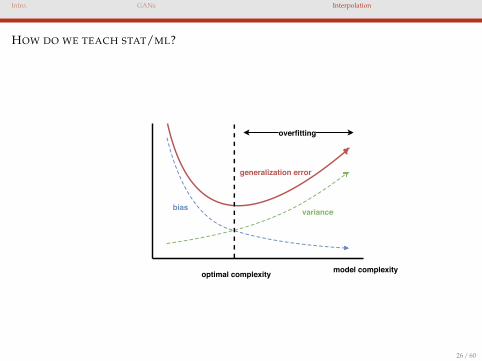
HOW DO WE TEACH STAT/ML?
model complexityoptimal complexity
bias variance
generalization error
overfitting
26 / 60
Intro. GANs Interpolation
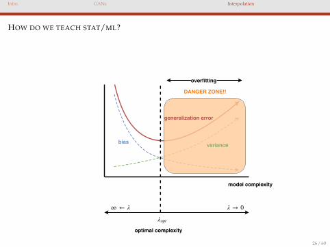
HOW DO WE TEACH STAT/ML?
model complexity
optimal complexity
bias variance
generalization error
overfitting
∞ ← λ λ → 0
λopt
DANGER ZONE!!
26 / 60
Intro. GANs Interpolation
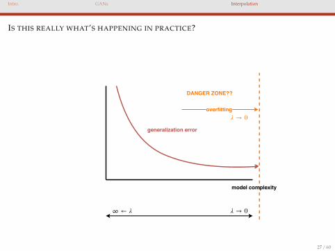
IS THIS REALLY WHAT’S HAPPENING IN PRACTICE?
model complexity
generalization error
overfitting
∞ ← λ
DANGER ZONE??
λ → 0
λ → 0
27 / 60

Intro. GANs Interpolation
Is explicit regularization λopt really needed?
Is interpolation really bad for statistics and machine learning?
28 / 60

Intro. GANs Interpolation
Is explicit regularization λopt really needed?
Is interpolation really bad for statistics and machine learning?
28 / 60
Intro. GANs Interpolation
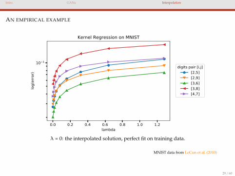
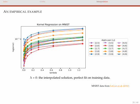
AN EMPIRICAL EXAMPLE
0.0 0.2 0.4 0.6 0.8 1.0 1.2lambda
10 1
log(
erro
r)Kernel Regression on MNIST
digits pair [i,j][2,5][2,9][3,6][3,8][4,7]
λ = 0: the interpolated solution, perfect fit on training data.
MNIST data from LeCun et al. (2010)
29 / 60
Intro. GANs Interpolation
AN EMPIRICAL EXAMPLE
0.0 0.2 0.4 0.6 0.8 1.0 1.2lambda
10 1
log(
erro
r)
Kernel Regression on MNIST
digits pair [i,j][2,5][2,6][2,7][2,8][2,9]
[3,5][3,6][3,7][3,8][3,9]
[4,5][4,6][4,7][4,8][4,9]
λ = 0: the interpolated solution, perfect fit on training data.
MNIST data from LeCun et al. (2010)
29 / 60
Intro. GANs Interpolation
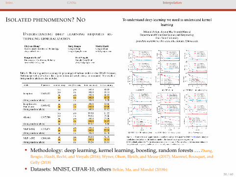
ISOLATED PHENOMENON? NO
• Methodology: deep learning, kernel learning, boosting, random forests . . . Zhang,Bengio, Hardt, Recht, and Vinyals (2016); Wyner, Olson, Bleich, and Mease (2017); Maennel, Bousquet, andGelly (2018)
• Datasets: MNIST, CIFAR-10, others Belkin, Ma, and Mandal (2018b)30 / 60

Intro. GANs Interpolation
PUZZLES
Interpolated solutions performs very well in practicefor many (modern) methodology and datasets!
What is happening? “Overfitting” is not that bad . . .
31 / 60
Intro. GANs Interpolation
OUR MESSAGE
Geometric properties of the data design X, high dimensionality, andcurvature of the kernel⇒ interpolated solution generalizes.
32 / 60

Intro. GANs Interpolation
Potential theory in statistics/learning for interpolated solution:
• Analysis through explicit regularization (7)• Capacity control (7)• Early stopping (algorithmic) (7)• Stability analysis (algorithmic) (7)• Nonparametric smoothing analysis (7)• Inductive bias (3?) at least promising
Belkin, Hsu, and Mitra (2018a)
33 / 60
Intro. GANs Interpolation
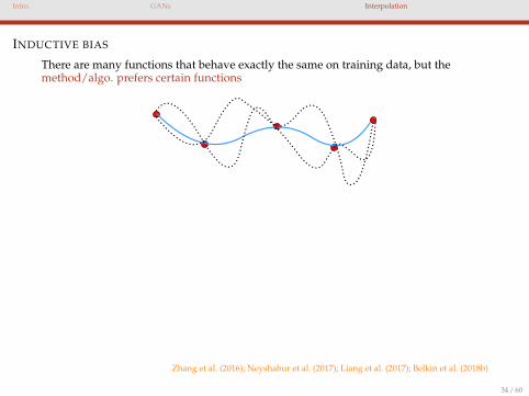
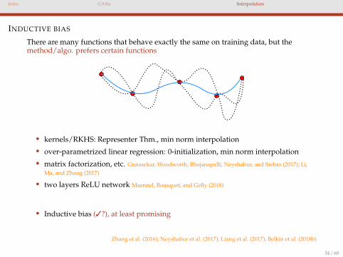
INDUCTIVE BIAS
There are many functions that behave exactly the same on training data, but themethod/algo. prefers certain functions
• kernels/RKHS: Representer Thm., min norm interpolation
• over-parametrized linear regression: 0-initialization, min norm interpolation
• matrix factorization, etc. Gunasekar, Woodworth, Bhojanapalli, Neyshabur, and Srebro (2017); Li,Ma, and Zhang (2017)
• two layers ReLU network Maennel, Bousquet, and Gelly (2018)
• Inductive bias (3?), at least promising
Zhang et al. (2016); Neyshabur et al. (2017); Liang et al. (2017); Belkin et al. (2018b)
34 / 60
Intro. GANs Interpolation
HISTORY: INTERPOLATION RULES
Understudied in the literature: especially when there is label noise
Recent progress on local/direct interpolation schemes:
• Geometric simplicial interpolation and weighted kNN Belkin, Hsu, and Mitra
(2018a)
• Nonparametric Nadaraya-Watson estimator with singular kernels Shepard
(1968); Devroye, Gyorfi, and Krzyzak (1998); Belkin, Rakhlin, and Tsybakov (2018c)
35 / 60
Intro. GANs Interpolation
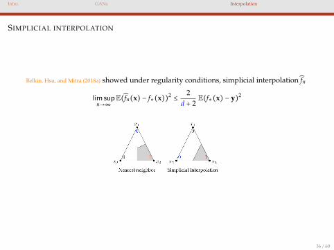
SIMPLICIAL INTERPOLATION
Belkin, Hsu, and Mitra (2018a) showed under regularity conditions, simplicial interpolation fn
lim supn→∞
E(fn(x) − f∗(x))2≤
2d + 2
E(f∗(x) − y)2
36 / 60
Intro. GANs Interpolation
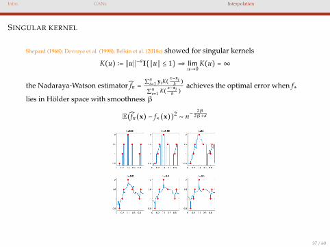
SINGULAR KERNEL
Shepard (1968); Devroye et al. (1998); Belkin et al. (2018c) showed for singular kernels
K(u) ∶= ∥u∥−aI∥u∥ ≤ 1⇒ limu→0
K(u) =∞
the Nadaraya-Watson estimator fn =∑n
i=1 yiK( x−xih )
∑ni=1 K( x−xi
h )achieves the optimal error when f∗
lies in Holder space with smoothness β
E(fn(x) − f∗(x))2∼ n−
2β2β+d
37 / 60
Intro. GANs Interpolation
Global/inverse interpolation methods (kernel machines/neuralnetworks/boosting) performs better than the local interpolation schemesempirically.
Several conjectures have been made about global/inverse interpolationmethods, such as kernel machines in Belkin, Hsu, and Mitra (2018a), two layers ReLUnets Maennel, Bousquet, and Gelly (2018).
38 / 60

Intro. GANs Interpolation
Interpolated min-norm solution for kernel ridge regression
39 / 60
Intro. GANs Interpolation
PROBLEM FORMULATION
Given n i.i.d. pairs (xi, yi) drawn from unknown µ: xi are d-dim covari-ates inΩ ⊂ Rd, yi ∈ R are the response/labels.
To estimate
f∗(x) = E(y∣x = x),
which is assumed to lie in a Reproducing Kernel Hilbert Space (RKHS)H with kernel K(⋅, ⋅).
Smola and Scholkopf (1998); Wahba (1990); Shawe-Taylor and Cristianini (2004)
40 / 60
Intro. GANs Interpolation
Conventional wisdom: Kernel Ridge Regression, explicit regularization λ ≠ 0added whenH is high- or infinite-dimensional
minf∈H
1n
n
∑i=1
(f(xi) − yi)2+ λ∥f∥2
H .
41 / 60
Intro. GANs Interpolation
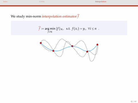
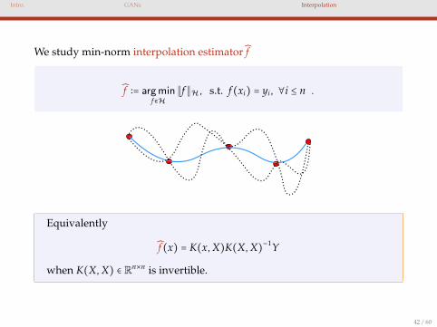
We study min-norm interpolation estimator f
f ∶= argminf∈H
∥f∥H, s.t. f(xi) = yi, ∀i ≤ n .
Equivalently
f(x) = K(x,X)K(X,X)−1Y
when K(X,X) ∈ Rn×n is invertible.
42 / 60
Intro. GANs Interpolation
We study min-norm interpolation estimator f
f ∶= argminf∈H
∥f∥H, s.t. f(xi) = yi, ∀i ≤ n .
Equivalently
f(x) = K(x,X)K(X,X)−1Y
when K(X,X) ∈ Rn×n is invertible.
42 / 60
Intro. GANs Interpolation
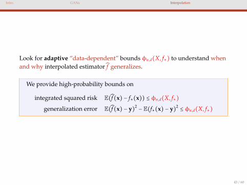
Look for adaptive “data-dependent” bounds φn,d(X, f∗) to understand whenand why interpolated estimator f generalizes.
We provide high-probability bounds on
integrated squared risk E(f(x) − f∗(x)) ≤ φn,d(X, f∗)
generalization error E(f(x) − y)2− E(f∗(x) − y)2
≤ φn,d(X, f∗)
43 / 60
Intro. GANs Interpolation
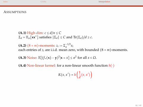
ASSUMPTIONS
(A.1) High-dim: c ≤ d/n ≤ CΣd = Eµ[xx∗] satisfies ∥Σd∥ ≤ C and Tr(Σd)/d ≥ c.
(A.2) (8 +m)-moments: zi ∶= Σ−1/2d xi
each entries of zi are i.i.d. mean zero, with bounded (8 +m)-moments.
(A.3) Noise: E[(f∗(x) − y)2∣x = x] ≤ σ2 for all x ∈Ω.
(A.4) Non-linear kernel: for a non-linear smooth function h(⋅)
K(x, x ′) = h(1d⟨x, x ′⟩)
44 / 60
Intro. GANs Interpolation
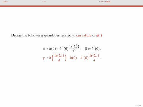
Define the following quantities related to curvature of h(⋅)
α ∶= h(0) + h ′′(0)Tr(Σ2
d)
d2, β ∶= h ′(0),
γ ∶= h(Tr(Σd)
d) − h(0) − h ′(0)
Tr(Σd)
d.
45 / 60
Intro. GANs Interpolation
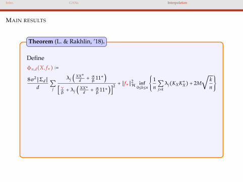
MAIN RESULTS
Define
φn,d(X, f∗) ∶=
8σ2∥Σd∥
d∑
j
λj (XX∗
d + αβ
11∗)
[γβ+ λj (
XX∗d + α
β11∗)]
2 + ∥f∗∥2H inf
0≤k≤n
⎧⎪⎪⎨⎪⎪⎩
1n∑j>kλj(KXK∗X) + 2M
√kn
⎫⎪⎪⎬⎪⎪⎭
Under (A.1)-(A.4), with prob. 1 − 2δ − d−2, interpolation estimator f
EY∣X ∥f − f∗∥2L2µ
EY∣X E(f(x) − y)2− E(f∗(x) − y)2
≤ φn,d(X, f∗) + ε(n, d).
The remainder term ε(n, d) = O(d−m
8+m log4.1 d) +O(n−12 log0.5(n/δ)).
Theorem (L. & Rakhlin, ’18).
46 / 60
Intro. GANs Interpolation
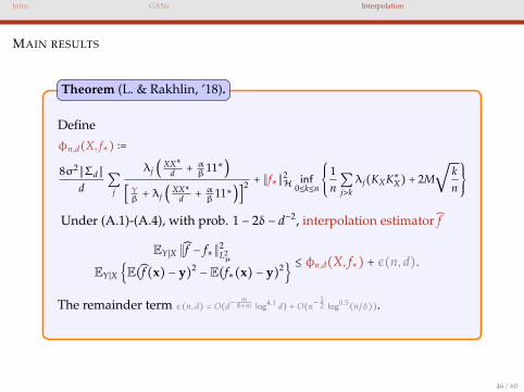
MAIN RESULTS
Define
φn,d(X, f∗) ∶=
8σ2∥Σd∥
d∑
j
λj (XX∗
d + αβ
11∗)
[γβ+ λj (
XX∗d + α
β11∗)]
2 + ∥f∗∥2H inf
0≤k≤n
⎧⎪⎪⎨⎪⎪⎩
1n∑j>kλj(KXK∗X) + 2M
√kn
⎫⎪⎪⎬⎪⎪⎭
Under (A.1)-(A.4), with prob. 1 − 2δ − d−2, interpolation estimator f
EY∣X ∥f − f∗∥2L2µ
EY∣X E(f(x) − y)2− E(f∗(x) − y)2
≤ φn,d(X, f∗) + ε(n, d).
The remainder term ε(n, d) = O(d−m
8+m log4.1 d) +O(n−12 log0.5(n/δ)).
Theorem (L. & Rakhlin, ’18).
46 / 60
Intro. GANs Interpolation
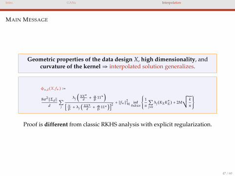
MAIN MESSAGE
Geometric properties of the data design X, high dimensionality, andcurvature of the kernel⇒ interpolated solution generalizes.
φn,d(X, f∗) ∶=
8σ2∥Σd∥d
∑j
λj ( XX∗d + α
β11∗)
[γβ+ λj ( XX∗
d + αβ
11∗)]2+ ∥f∗∥2
H inf0≤k≤n
⎧⎪⎪⎪⎨⎪⎪⎪⎩
1
n∑j>kλj(KXK∗X) + 2M
¿ÁÁÀ k
n
⎫⎪⎪⎪⎬⎪⎪⎪⎭
Proof is different from classic RKHS analysis with explicit regularization.
47 / 60
Intro. GANs Interpolation
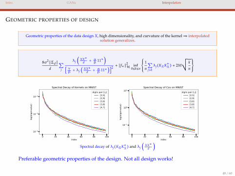
GEOMETRIC PROPERTIES OF DESIGN
Geometric properties of the data design X, high dimensionality, and curvature of the kernel⇒ interpolatedsolution generalizes.
8σ2∥Σd∥d
∑j
λj ( XX∗d + α
β11∗)
[γβ+ λj ( XX∗
d + αβ
11∗)]2+ ∥f∗∥2
H inf0≤k≤n
⎧⎪⎪⎪⎨⎪⎪⎪⎩
1
n∑j>kλj(KXK∗X) + 2M
¿ÁÁÀ k
n
⎫⎪⎪⎪⎬⎪⎪⎪⎭
0 20 40 60 80 100index
10 4
10 3
10 2
log(
eige
nval
ue)
Spectral Decay of Kernels on MNISTdigits pair [i,j]
[2,5][2,9][3,6][3,8][4,7]
0 20 40 60 80 100index
10 1
100
101
log(
eige
nval
ue)
Spectral Decay of Cov on MNISTdigits pair [i,j]
[2,5][2,9][3,6][3,8][4,7]
Spectral decay of λj(KXK∗X) and λj ( XX∗d )
Preferable geometric properties of the design. Not all design works!
48 / 60
Intro. GANs Interpolation
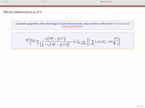
HIGH DIMENSIONALITY
Geometric properties of the data design X, high dimensionality, and curvature of the kernel⇒ interpolatedsolution generalizes.
8σ2∥Σd∥d
∑j
λj ( XX∗d + α
β11∗)
[γβ+ λj ( XX∗
d + αβ
11∗)]2+ ∥f∗∥2
H inf0≤k≤n
⎧⎪⎪⎪⎨⎪⎪⎪⎩
1
n∑j>kλj(KXK∗X) + 2M
¿ÁÁÀ k
n
⎫⎪⎪⎪⎬⎪⎪⎪⎭
Scalings:• c < d/n < C, typical high-dim scaling in RMT, El Karoui (2010); Johnstone (2001)
• scaling: K(x, x ′) = h(⟨x, x ′⟩/d), default choice for high dim. data in computingpackages, e.g. Scikit-learn Pedregosa et al. (2011)
• bounds work for large (d,n) regime,ε(n, d) = O(d−m/(8+m) log4.1 d) +O(n−1/2 log0.5(n/δ))
Blessings of high dimensionality:• similar effect observed in local/direct interpolating schemes in Belkin et al. (2018a)
for simplicial interpolation and weighted kNN
• Kernel “ridgeless” regression is a global/inverse interpolation scheme
49 / 60
Intro. GANs Interpolation
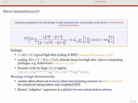
HIGH DIMENSIONALITY
Geometric properties of the data design X, high dimensionality, and curvature of the kernel⇒ interpolatedsolution generalizes.
8σ2∥Σd∥d
∑j
λj ( XX∗d + α
β11∗)
[γβ+ λj ( XX∗
d + αβ
11∗)]2+ ∥f∗∥2
H inf0≤k≤n
⎧⎪⎪⎪⎨⎪⎪⎪⎩
1
n∑j>kλj(KXK∗X) + 2M
¿ÁÁÀ k
n
⎫⎪⎪⎪⎬⎪⎪⎪⎭
Scalings:• c < d/n < C, typical high-dim scaling in RMT, El Karoui (2010); Johnstone (2001)
• scaling: K(x, x ′) = h(⟨x, x ′⟩/d), default choice for high dim. data in computingpackages, e.g. Scikit-learn Pedregosa et al. (2011)
• bounds work for large (d,n) regime,ε(n, d) = O(d−m/(8+m) log4.1 d) +O(n−1/2 log0.5(n/δ))
Blessings of high dimensionality:• similar effect observed in local/direct interpolating schemes in Belkin et al. (2018a)
for simplicial interpolation and weighted kNN
• Kernel “ridgeless” regression is a global/inverse interpolation scheme
49 / 60
Intro. GANs Interpolation
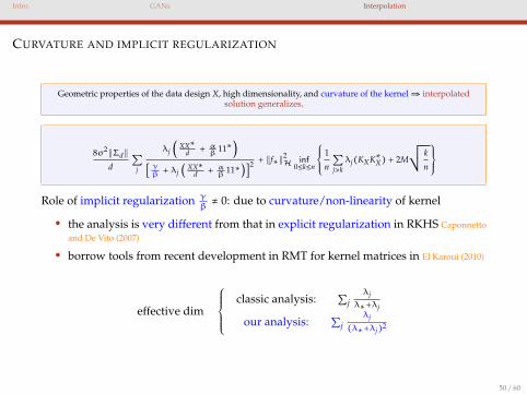
CURVATURE AND IMPLICIT REGULARIZATION
Geometric properties of the data design X, high dimensionality, and curvature of the kernel⇒ interpolatedsolution generalizes.
8σ2∥Σd∥d
∑j
λj ( XX∗d + α
β11∗)
[γβ+ λj ( XX∗
d + αβ
11∗)]2+ ∥f∗∥2
H inf0≤k≤n
⎧⎪⎪⎪⎨⎪⎪⎪⎩
1
n∑j>kλj(KXK∗X) + 2M
¿ÁÁÀ k
n
⎫⎪⎪⎪⎬⎪⎪⎪⎭
Role of implicit regularization γβ≠ 0: due to curvature/non-linearity of kernel
• the analysis is very different from that in explicit regularization in RKHS Caponnettoand De Vito (2007)
• borrow tools from recent development in RMT for kernel matrices in El Karoui (2010)
effective dim
⎧⎪⎪⎪⎪⎨⎪⎪⎪⎪⎩
classic analysis: ∑jλj
λ∗+λj
our analysis: ∑jλj
(λ∗+λj)2
50 / 60
Intro. GANs Interpolation
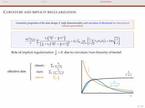
CURVATURE AND IMPLICIT REGULARIZATION
Geometric properties of the data design X, high dimensionality, and curvature of the kernel⇒ interpolatedsolution generalizes.
8σ2∥Σd∥d
∑j
λj ( XX∗d + α
β11∗)
[γβ+ λj ( XX∗
d + αβ
11∗)]2+ ∥f∗∥2
H inf0≤k≤n
⎧⎪⎪⎪⎨⎪⎪⎪⎩
1
n∑j>kλj(KXK∗X) + 2M
¿ÁÁÀ k
n
⎫⎪⎪⎪⎬⎪⎪⎪⎭
Role of implicit regularization γβ≠ 0: due to curvature/non-linearity of kernel
effective dim
⎧⎪⎪⎪⎪⎪⎪⎪⎨⎪⎪⎪⎪⎪⎪⎪⎩
classic: ∑jλj
λ∗+λj
ours: ∑jλj
(λ∗+λj)2
naive: ∑j1λj
λj
λj
+λ⋅
λj
λj
( + )λ⋅
λj
2
1
λj
51 / 60
Intro. GANs Interpolation
MAIN MESSAGE
Geometric properties of the data design X, high dimensionality, andcurvature of the kernel⇒ interpolated solution generalizes.
“implicit regularization” + “inductive bias”
52 / 60

Intro. GANs Interpolation
“Explicit regularization may improve generalization performance, but is neithernecessary nor by itself sufficient for controlling generalization error.”
— Zhang, Bengio, Hardt, Recht, and Vinyals (2016)
53 / 60

Intro. GANs Interpolation
Gradient descent on two layers ReLU Networks
54 / 60
Intro. GANs Interpolation
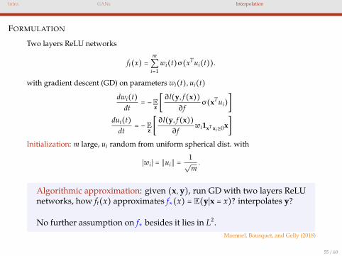
FORMULATION
Two layers ReLU networks
ft(x) =m∑i=1
wi(t)σ(xTui(t)).
with gradient descent (GD) on parameters wi(t),ui(t)
dwi(t)dt
= −Ez[∂l(y, f(x))
∂fσ(xTui)]
dui(t)dt
= −Ez[∂l(y, f(x))
∂fwi1xTui≥0x]
Initialization: m large, ui random from uniform spherical dist. with
∣wi∣ = ∥ui∥ =1
√m.
Algorithmic approximation: given (x,y), run GD with two layers ReLUnetworks, how ft(x) approximates f∗(x) = E(y∣x = x)? interpolates y?
No further assumption on f∗ besides it lies in L2.Maennel, Bousquet, and Gelly (2018)
55 / 60
Intro. GANs Interpolation
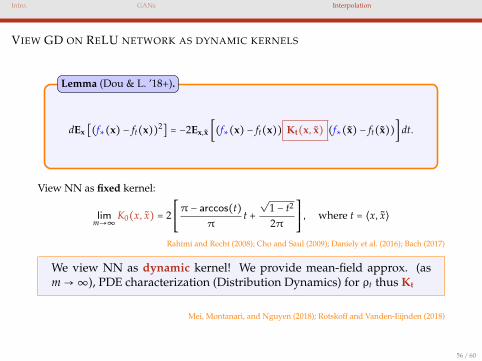
VIEW GD ON RELU NETWORK AS DYNAMIC KERNELS
dEx [(f∗(x) − ft(x))2] = −2Ex,x [(f∗(x) − ft(x)) Kt(x, x) (f∗(x) − ft(x))] dt.
Lemma (Dou & L. ’18+).
View NN as fixed kernel:
limm→∞
K0(x, x) = 2⎡⎢⎢⎢⎢⎣
π − arccos(t)π
t +
√1 − t2
2π
⎤⎥⎥⎥⎥⎦
, where t = ⟨x, x⟩
Rahimi and Recht (2008); Cho and Saul (2009); Daniely et al. (2016); Bach (2017)
We view NN as dynamic kernel! We provide mean-field approx. (asm→∞), PDE characterization (Distribution Dynamics) for ρt thus Kt
Mei, Montanari, and Nguyen (2018); Rotskoff and Vanden-Eijnden (2018)
56 / 60

Intro. GANs Interpolation
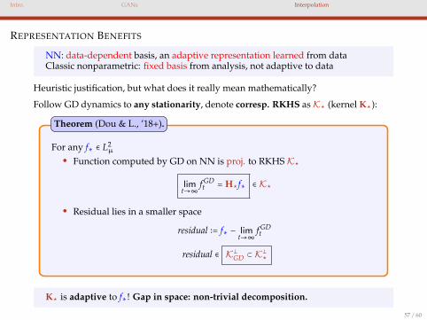
REPRESENTATION BENEFITS
NN: data-dependent basis, an adaptive representation learned from dataClassic nonparametric: fixed basis from analysis, not adaptive to data
Heuristic justification, but what does it really mean mathematically?
Follow GD dynamics to any stationarity, denote corresp. RKHS asK⋆ (kernel K⋆):
For any f∗ ∈ L2µ
• Function computed by GD on NN is proj. to RKHS K⋆
limt→∞
f GDt = H⋆f∗ ∈ K⋆
• Residual lies in a smaller space
residual ∶= f∗ − limt→∞
f GDt
residual ∈ K⊥GD ⊂ K⊥⋆
Theorem (Dou & L., ’18+).
K⋆ is adaptive to f∗! Gap in space: non-trivial decomposition.
57 / 60
Intro. GANs Interpolation
INTERPOLATION BENEFITS
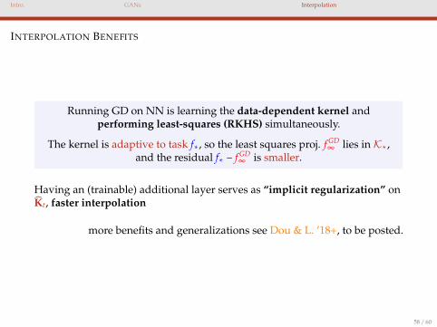
Running GD on NN is learning the data-dependent kernel andperforming least-squares (RKHS) simultaneously.
The kernel is adaptive to task f∗, so the least squares proj. f GD∞ lies in K⋆,
and the residual f∗ − f GD∞ is smaller.
Having an (trainable) additional layer serves as “implicit regularization” onKt, faster interpolation
more benefits and generalizations see Dou & L. ’18+, to be posted.
58 / 60
Intro. GANs Interpolation
CONCLUSION
• Minimax optimal rates does not explain the empirical success of neuralnetworks.
• One needs new adaptive (to properties of data), data-dependentframework/understanding.
• Requires new insights on regularization and interpolation.
image credit to Internet
59 / 60
References
Thank you!
Liang, T. (2018). — On How Well Generative Adversarial Networks Learn Densities: Nonparametric and
Parametric Results. available on arXiv:1811.03179 under review
Liang, T. & Rakhlin, A. (2018). — Just Interpolate: Kernel “Ridgeless” Regression Can Generalize. available
on arXiv:1808.00387 revision invited
Liang, T. & Stokes, J. (2018). — Interaction Matters: A Note on Non-asymptotic Local Convergence of
Generative Adversarial Networks. available on arXiv:1802.06132 AISTATS 2019, to appear
Liang, T., Poggio, T., Rakhlin, A. & Stokes, J. (2017). — Fisher-Rao Metric, Geometry, and Complexity of
Neural Networks. available on arXiv:1711.01530 AISTATS 2019, to appear
Dou, X. & Liang, T. (2018+). — Training Neural Networks as Learning Data-adaptive Kernels: Provable
Representation and Approximation Benefits. available on hereMichael Arbel, Dougal J Sutherland, Mikołaj Binkowski, and Arthur Gretton. On gradient regularizers for mmd gans. arXiv preprint
arXiv:1805.11565, 2018.Martin Arjovsky and Leon Bottou. Towards principled methods for training generative adversarial networks. arXiv preprint
arXiv:1701.04862, 2017.Martin Arjovsky, Soumith Chintala, and Leon Bottou. Wasserstein gan. arXiv preprint arXiv:1701.07875, 2017.Sanjeev Arora and Yi Zhang. Do gans actually learn the distribution? an empirical study. arXiv preprint arXiv:1706.08224, 2017.Sanjeev Arora, Rong Ge, Yingyu Liang, Tengyu Ma, and Yi Zhang. Generalization and equilibrium in generative adversarial nets (gans).
arXiv preprint arXiv:1703.00573, 2017a.Sanjeev Arora, Andrej Risteski, and Yi Zhang. Theoretical limitations of encoder-decoder gan architectures. arXiv preprint arXiv:1711.02651,
2017b.Francis Bach. Breaking the curse of dimensionality with convex neural networks. Journal of Machine Learning Research, 18(19):1–53, 2017.Yu Bai, Tengyu Ma, and Andrej Risteski. Approximability of discriminators implies diversity in gans. arXiv preprint arXiv:1806.10586, 2018.Mikhail Belkin, Daniel Hsu, and Partha Mitra. Overfitting or perfect fitting? risk bounds for classification and regression rules that
interpolate. arXiv preprint arXiv:1806.05161, 2018a.Mikhail Belkin, Siyuan Ma, and Soumik Mandal. To understand deep learning we need to understand kernel learning. arXiv preprint
arXiv:1802.01396, 2018b.Mikhail Belkin, Alexander Rakhlin, and Alexandre B Tsybakov. Does data interpolation contradict statistical optimality? arXiv preprint
arXiv:1806.09471, 2018c.Guillermo Canas and Lorenzo Rosasco. Learning probability measures with respect to optimal transport metrics. In Advances in Neural
Information Processing Systems, pages 2492–2500, 2012.Andrea Caponnetto and Ernesto De Vito. Optimal rates for the regularized least-squares algorithm. Foundations of Computational
Mathematics, 7(3):331–368, 2007.Youngmin Cho and Lawrence K Saul. Kernel methods for deep learning. In Advances in neural information processing systems, pages 342–350,
2009.Amit Daniely, Roy Frostig, and Yoram Singer. Toward deeper understanding of neural networks: The power of initialization and a dual
view on expressivity. In Advances In Neural Information Processing Systems, pages 2253–2261, 2016.Constantinos Daskalakis, Andrew Ilyas, Vasilis Syrgkanis, and Haoyang Zeng. Training gans with optimism. arXiv preprint
arXiv:1711.00141, 2017.Luc Devroye, Laszlo Gyorfi, and Adam Krzyzak. The hilbert kernel regression estimate. Journal of Multivariate Analysis, 65(2):209–227, 1998.Gintare Karolina Dziugaite, Daniel M Roy, and Zoubin Ghahramani. Training generative neural networks via maximum mean discrepancy
optimization. arXiv preprint arXiv:1505.03906, 2015.Noureddine El Karoui. The spectrum of kernel random matrices. The Annals of Statistics, 38(1):1–50, 2010.Ian Goodfellow, Jean Pouget-Abadie, Mehdi Mirza, Bing Xu, David Warde-Farley, Sherjil Ozair, Aaron Courville, and Yoshua Bengio.
Generative adversarial nets. In Advances in neural information processing systems, pages 2672–2680, 2014.Suriya Gunasekar, Blake E Woodworth, Srinadh Bhojanapalli, Behnam Neyshabur, and Nati Srebro. Implicit regularization in matrix
factorization. In Advances in Neural Information Processing Systems, pages 6151–6159, 2017.Iain M Johnstone. On the distribution of the largest eigenvalue in principal components analysis. Annals of statistics, pages 295–327, 2001.Yann LeCun, Corinna Cortes, and CJ Burges. Mnist handwritten digit database. AT&T Labs [Online]. Available: http://yann. lecun.
com/exdb/mnist, 2, 2010.Yuanzhi Li, Tengyu Ma, and Hongyang Zhang. Algorithmic regularization in over-parameterized matrix recovery. arXiv preprint
arXiv:1712.09203, 2017.Yujia Li, Kevin Swersky, and Rich Zemel. Generative moment matching networks. In Proceedings of the 32nd International Conference on
Machine Learning (ICML-15), pages 1718–1727, 2015.Tengyuan Liang. How well can generative adversarial networks learn densities: A nonparametric view. arXiv preprint arXiv:1712.08244,
2017.Tengyuan Liang, Tomaso Poggio, Alexander Rakhlin, and James Stokes. Fisher-rao metric, geometry, and complexity of neural networks.
arXiv preprint arXiv:1711.01530, 2017.Shuang Liu, Olivier Bousquet, and Kamalika Chaudhuri. Approximation and convergence properties of generative adversarial learning.
arXiv preprint arXiv:1705.08991, 2017.Hartmut Maennel, Olivier Bousquet, and Sylvain Gelly. Gradient descent quantizes relu network features. arXiv preprint arXiv:1803.08367,
2018.Bernard A Mair and Frits H Ruymgaart. Statistical inverse estimation in hilbert scales. SIAM Journal on Applied Mathematics, 56(5):
1424–1444, 1996.Song Mei, Andrea Montanari, and Phan-Minh Nguyen. A mean field view of the landscape of two-layers neural networks. arXiv preprint
arXiv:1804.06561, 2018.Lars Mescheder, Andreas Geiger, and Sebastian Nowozin. Which training methods for gans do actually converge? In International
Conference on Machine Learning, pages 3478–3487, 2018.Youssef Mroueh, Chun-Liang Li, Tom Sercu, Anant Raj, and Yu Cheng. Sobolev gan. arXiv preprint arXiv:1711.04894, 2017.A Nemirovski and D Yudin. Information-based complexity of mathematical programming. Izvestia AN SSSR, Ser. Tekhnicheskaya Kibernetika
(the journal is translated to English as Engineering Cybernetics. Soviet J. Computer & Systems Sci.), 1, 1983.Arkadi Nemirovski. Topics in non-parametric. Ecole d’Ete de Probabilites de Saint-Flour, 28:85, 2000.Yurii Nesterov. Introductory lectures on convex optimization: A basic course, volume 87. Springer Science & Business Media, 2013.Behnam Neyshabur, Srinadh Bhojanapalli, David McAllester, and Nati Srebro. Exploring generalization in deep learning. In Advances in
Neural Information Processing Systems, pages 5947–5956, 2017.Sebastian Nowozin, Botond Cseke, and Ryota Tomioka. f-gan: Training generative neural samplers using variational divergence
minimization. In Advances in Neural Information Processing Systems, pages 271–279, 2016.F. Pedregosa, G. Varoquaux, A. Gramfort, V. Michel, B. Thirion, O. Grisel, M. Blondel, P. Prettenhofer, R. Weiss, V. Dubourg, J. Vanderplas,
A. Passos, D. Cournapeau, M. Brucher, M. Perrot, and E. Duchesnay. Scikit-learn: Machine learning in Python. Journal of MachineLearning Research, 12:2825–2830, 2011.
David Pfau and Oriol Vinyals. Connecting generative adversarial networks and actor-critic methods. arXiv preprint arXiv:1610.01945, 2016.Ali Rahimi and Benjamin Recht. Random features for large-scale kernel machines. In Advances in neural information processing systems, pages
1177–1184, 2008.Grant M Rotskoff and Eric Vanden-Eijnden. Neural networks as interacting particle systems: Asymptotic convexity of the loss landscape
and universal scaling of the approximation error. arXiv preprint arXiv:1805.00915, 2018.Tim Salimans, Ian Goodfellow, Wojciech Zaremba, Vicki Cheung, Alec Radford, and Xi Chen. Improved techniques for training gans. In
Advances in Neural Information Processing Systems, pages 2234–2242, 2016.John Shawe-Taylor and Nello Cristianini. Kernel methods for pattern analysis. Cambridge university press, 2004.Donald Shepard. A two-dimensional interpolation function for irregularly-spaced data. In Proceedings of the 1968 23rd ACM national
conference, pages 517–524. ACM, 1968.Satinder Singh, Michael Kearns, and Yishay Mansour. Nash convergence of gradient dynamics in general-sum games. In Proceedings of the
Sixteenth conference on Uncertainty in artificial intelligence, pages 541–548. Morgan Kaufmann Publishers Inc., 2000.Shashank Singh, Ananya Uppal, Boyue Li, Chun-Liang Li, Manzil Zaheer, and Barnabas Poczos. Nonparametric density estimation under
adversarial losses. arXiv preprint arXiv:1805.08836, 2018.Alex J Smola and Bernhard Scholkopf. Learning with kernels, volume 4. Citeseer, 1998.Casper Kaae Sønderby, Jose Caballero, Lucas Theis, Wenzhe Shi, and Ferenc Huszar. Amortised map inference for image super-resolution.
arXiv preprint arXiv:1610.04490, 2016.Charles J Stone. Optimal global rates of convergence for nonparametric regression. The annals of statistics, pages 1040–1053, 1982.Ilya O Tolstikhin, Sylvain Gelly, Olivier Bousquet, Carl-Johann Simon-Gabriel, and Bernhard Scholkopf. Adagan: Boosting generative
models. In Advances in Neural Information Processing Systems, pages 5424–5433, 2017.Alexandre B Tsybakov. Introduction to nonparametric estimation. Springer Series in Statistics. Springer, New York, 2009.Grace Wahba. Spline models for observational data, volume 59. Siam, 1990.Larry Wassermann. All of nonparametric statistics. Springer Science+ Business Media, New York, 2006.Abraham J Wyner, Matthew Olson, Justin Bleich, and David Mease. Explaining the success of adaboost and random forests as interpolating
classifiers. The Journal of Machine Learning Research, 18(1):1558–1590, 2017.Chiyuan Zhang, Samy Bengio, Moritz Hardt, Benjamin Recht, and Oriol Vinyals. Understanding deep learning requires rethinking
generalization. arXiv preprint arXiv:1611.03530, 2016.
60 / 60


![WCDA Regularization for 3D Quantitative Microwave Tomography · WCDA Regularization for 3D Quantitative Microwave Tomography 2 problem is also ill-posed [11] and regularization is](https://img.pdfslide.us/doc/110x75/5e3abb0a2129886ec2199ead/wcda-regularization-for-3d-quantitative-microwave-tomography-wcda-regularization.jpg)