The Green Revolution and Infant Mortality

Evidence from 600,000 Births

Prabhat Barnwal1, Aaditya Dar2, Jan von der Goltz3, Ram Fishman4,

Gordon McCord5 and Nathan Mueller6

July 30, 2016

1Michigan State University, 2George Washington University, 3World Bank, 4Tel Aviv

University, 5University of California, San Diego and 6Harvard University

1/43

Outline

Motivation

Data

Outcomes

Crop area

Improved Varieties

Empirical Strategy

Findings

Impact of MVs

DIIVA (MV Releases)

GAEZ

Country Case Study

2/43

Motivation

Motivation

• The Green Revolution is arguably one of the most significanteconomic transformations of the 20th century• More than 8,000 modern varieties (MVs) released over the

past 40 years and sown over much of the global cultivated area

(World Bank, 2008)

• Thought to have led to major improvements in productivity,

income, food security and health in developing countries

(Evenson and Gollin, 2003; Bustos et al., 2016; McArthur and

McCord, 2016)• In recent years, renewed debate on:

• The role of agriculture in development

• The impact of agricultural productivity gains on food security,

nutrition and health

• The efficient levels of public investment in agricultural R&D

and technology diffusion3/43

Infant Mortality and MV Adoption, by region

0

.05

.1

.15

.2In

fant

Mor

talit

y (in

%)

1960− 1970− 1980− 1990− 2000−Decade

0

.2

.4

.6

Are

a w

eigh

ted

MV

ado

ptio

n (in

%)

1960 1970 1980 1990 2000Year

LAC MENA SSA SSEA

4/43

Motivation

• Estimating the causal impact of the GR is challenging:

• Large scale, gradual transformation

• Severe data limitations

• (Development and) Adoption of MVs is endogenous, creating

potentially spurious correlations with economic or health

outcomes.

• Large potential spillover effects.

5/43

Motivation

• Most evidence limited to:

• Mostly country level correlations (including panels) of MV

adoption and agricultural productivity (Evenson and Gollin,

2003; Walker and Alwang, 2015)

• Relatively small number of experimental or quasi-experimental

localised studies of impacts on food security (Stewart et al,

2015)

• Country level relationships could be biased by various policy

and economic confounders.

• At the country level, no evidence for negative relationship

between infant mortality and MV diffusion.

6/43

This Paper

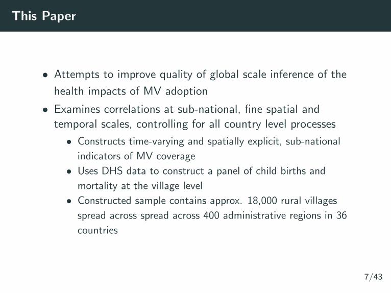
• Attempts to improve quality of global scale inference of the

health impacts of MV adoption

• Examines correlations at sub-national, fine spatial andtemporal scales, controlling for all country level processes

• Constructs time-varying and spatially explicit, sub-national

indicators of MV coverage

• Uses DHS data to construct a panel of child births and

mortality at the village level

• Constructed sample contains approx. 18,000 rural villages

spread across spread across 400 administrative regions in 36

countries

7/43

Data

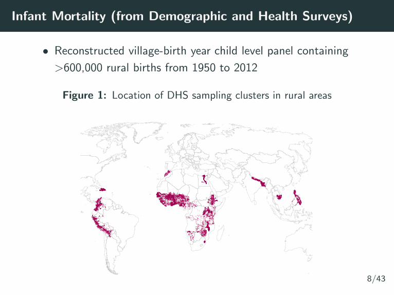
Infant Mortality (from Demographic and Health Surveys)

• Reconstructed village-birth year child level panel containing

>600,000 rural births from 1950 to 2012

Figure 1: Location of DHS sampling clusters in rural areas

8/43

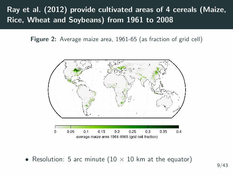
Ray et al. (2012) provide cultivated areas of 4 cereals (Maize,

Rice, Wheat and Soybeans) from 1961 to 2008

Figure 2: Average maize area, 1961-65 (as fraction of grid cell)

• Resolution: 5 arc minute (10 × 10 km at the equator)9/43

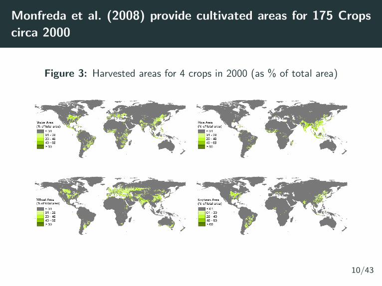
Monfreda et al. (2008) provide cultivated areas for 175 Crops

circa 2000

Figure 3: Harvested areas for 4 crops in 2000 (as % of total area)

10/43

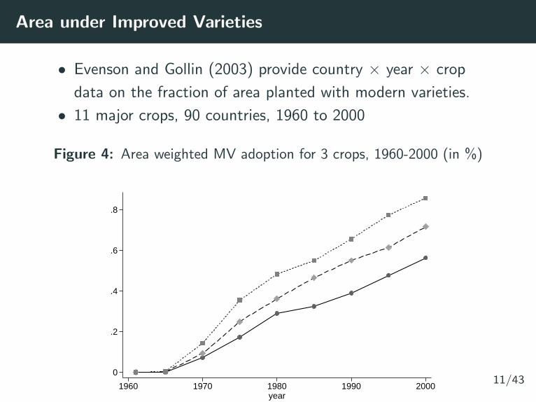
Area under Improved Varieties

• Evenson and Gollin (2003) provide country × year × crop

data on the fraction of area planted with modern varieties.

• 11 major crops, 90 countries, 1960 to 2000

Figure 4: Area weighted MV adoption for 3 crops, 1960-2000 (in %)

0

.2

.4

.6

.8

1960 1970 1980 1990 2000year

Maize Rice Wheat

11/43

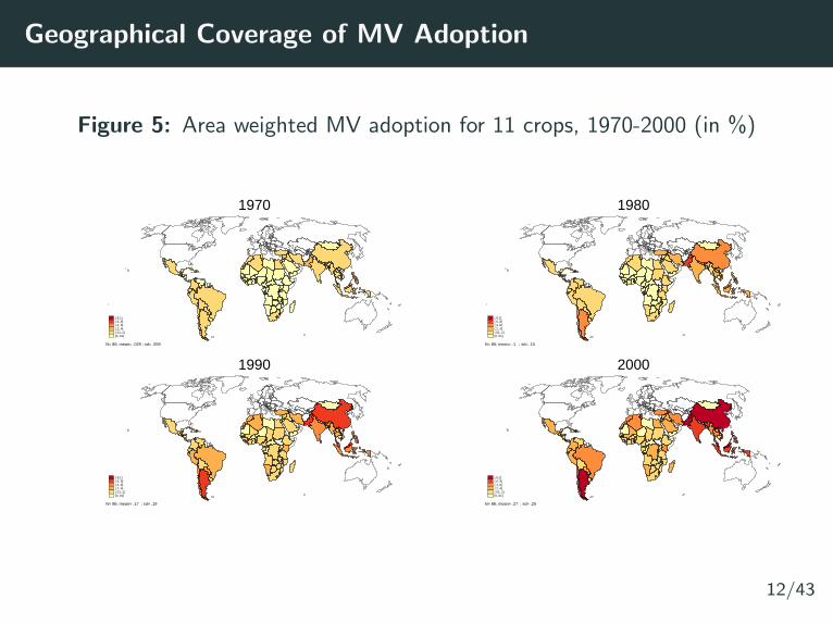
Geographical Coverage of MV Adoption

Figure 5: Area weighted MV adoption for 11 crops, 1970-2000 (in %)

(.8,1](.6,.8](.4,.6](.2,.4](.01,.2][0,.01]

N= 86; mean= .029 ; sd= .059

1970

(.8,1](.6,.8](.4,.6](.2,.4](.01,.2][0,.01]

N= 86; mean= .1 ; sd= .15

1980

(.8,1](.6,.8](.4,.6](.2,.4](.01,.2][0,.01]

N= 86; mean= .17 ; sd= .19

1990

(.8,1](.6,.8](.4,.6](.2,.4](.01,.2][0,.01]

N= 86; mean= .27 ; sd= .25

2000

12/43

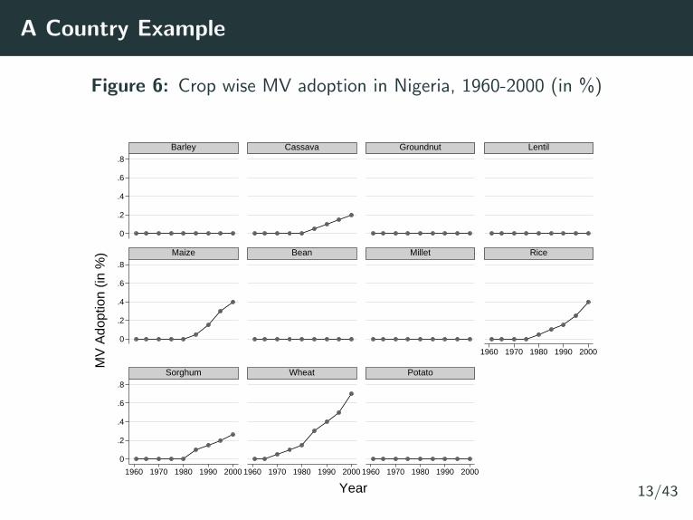
A Country Example

Figure 6: Crop wise MV adoption in Nigeria, 1960-2000 (in %)

0

.2

.4

.6

.8

0

.2

.4

.6

.8

0

.2

.4

.6

.8

1960 1970 1980 1990 2000

1960 1970 1980 1990 2000 1960 1970 1980 1990 2000 1960 1970 1980 1990 2000

Barley Cassava Groundnut Lentil

Maize Bean Millet Rice

Sorghum Wheat Potato

MV

Ado

ptio

n (in

%)

Year 13/43

Empirical Strategy

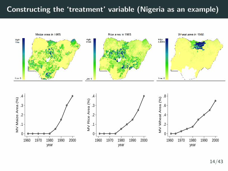
Constructing the ‘treatment’ variable (Nigeria as an example)

0

.1

.2

.3

.4

MV

Ma

ize

Are

a (

%)

1960 1970 1980 1990 2000year

0

.1

.2

.3

.4

MV

Ric

e A

rea

(%

)

1960 1970 1980 1990 2000year

0

.2

.4

.6

.8

MV

Wh

ea

t A

rea

(%

)

1960 1970 1980 1990 2000year

14/43

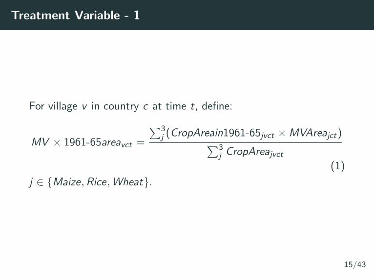
Treatment Variable - 1

For village v in country c at time t, define:

MV × 1961-65areavct =

∑3j (CropAreain1961-65jvct ×MVAreajct)∑3

j CropAreajvct(1)

j ∈ {Maize,Rice,Wheat}.

15/43

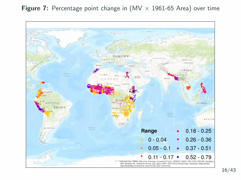
Figure 7: Percentage point change in (MV × 1961-65 Area) over time

Sources: Esri, HERE, DeLorme, Intermap, increment P Corp., GEBCO, USGS, FAO, NPS, NRCAN, GeoBase,IGN, Kadaster NL, Ordnance Survey, Esri Japan, METI, Esri China (Hong Kong), swisstopo, MapmyIndia, 'OpenStreetMap contributors, and the GIS User Community

0 - 0.04

0.05 - 0.1

0.11 - 0.17

Range 0.18 - 0.25

0.26 - 0.36

0.37 - 0.51

0.52 - 0.79

16/43

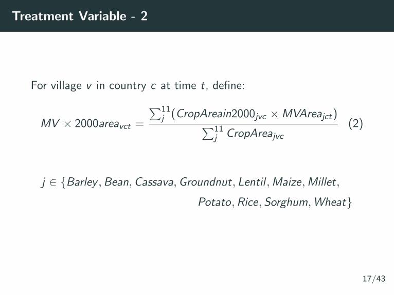
Treatment Variable - 2

For village v in country c at time t, define:

MV × 2000areavct =

∑11j (CropAreain2000jvc ×MVAreajct)∑11

j CropAreajvc(2)

j ∈ {Barley ,Bean,Cassava,Groundnut, Lentil ,Maize,Millet,

Potato,Rice,Sorghum,Wheat}

17/43

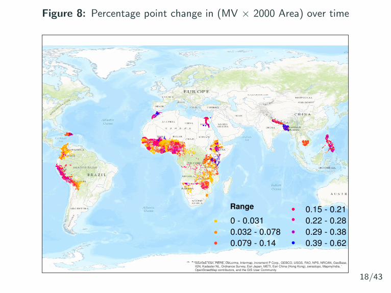
Figure 8: Percentage point change in (MV × 2000 Area) over time

Sources: Esri, HERE, DeLorme, Intermap, increment P Corp., GEBCO, USGS, FAO, NPS, NRCAN, GeoBase,IGN, Kadaster NL, Ordnance Survey, Esri Japan, METI, Esri China (Hong Kong), swisstopo, MapmyIndia, 'OpenStreetMap contributors, and the GIS User Community

Range

0 - 0.031

0.032 - 0.078

0.079 - 0.14

0.15 - 0.21

0.22 - 0.28

0.29 - 0.38

0.39 - 0.62

18/43

Identification Strategy

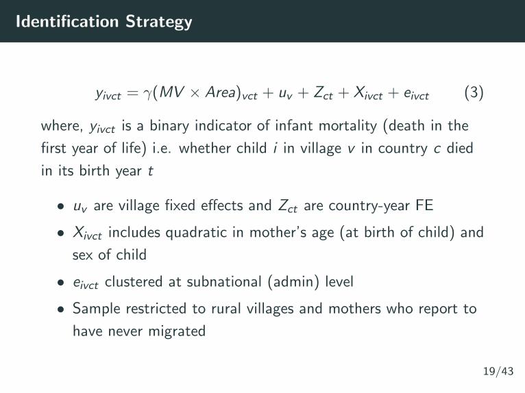
yivct = γ(MV × Area)vct + uv + Zct + Xivct + eivct (3)

where, yivct is a binary indicator of infant mortality (death in the

first year of life) i.e. whether child i in village v in country c died

in its birth year t

• uv are village fixed effects and Zct are country-year FE

• Xivct includes quadratic in mother’s age (at birth of child) and

sex of child

• eivct clustered at subnational (admin) level

• Sample restricted to rural villages and mothers who report to

have never migrated

19/43

Identification Strategy

• Examines whether parts of the country where MVs were faster

adopted display faster than average reductions in infant

mortality

• Controlling for flexible country × birth year FE absorbs all

economic and policy changes at the country level

• Only identifies effects occurring due to:

• Income increases for farmers

• Localised increases in food availability resulting from limited

market connectivity

20/43

Concerns re Identification

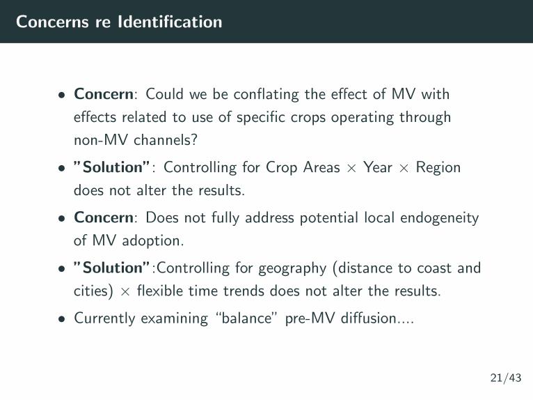
• Concern: Could we be conflating the effect of MV with

effects related to use of specific crops operating through

non-MV channels?

• ”Solution”: Controlling for Crop Areas × Year × Region

does not alter the results.

• Concern: Does not fully address potential local endogeneity

of MV adoption.

• ”Solution”:Controlling for geography (distance to coast and

cities) × flexible time trends does not alter the results.

• Currently examining “balance” pre-MV diffusion....

21/43

Findings

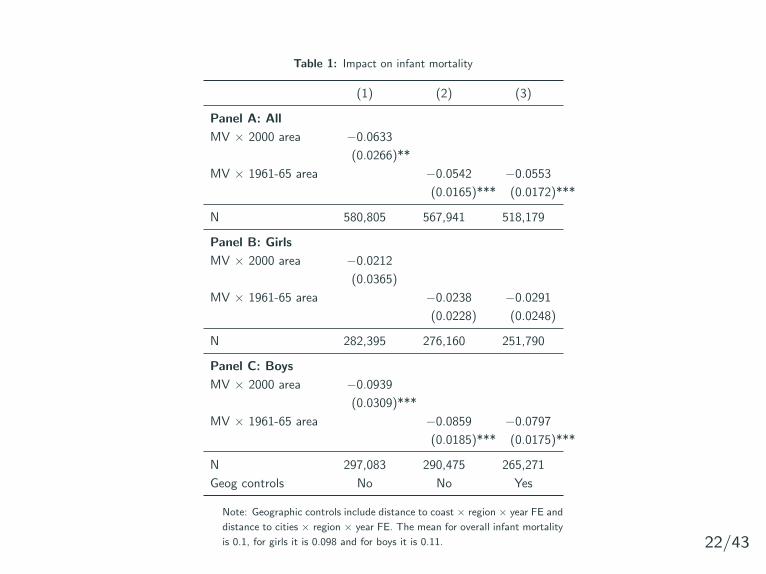
Table 1: Impact on infant mortality

(1) (2) (3)

Panel A: All

MV × 2000 area −0.0633

(0.0266)**

MV × 1961-65 area −0.0542 −0.0553

(0.0165)*** (0.0172)***

N 580,805 567,941 518,179

Panel B: Girls

MV × 2000 area −0.0212

(0.0365)

MV × 1961-65 area −0.0238 −0.0291

(0.0228) (0.0248)

N 282,395 276,160 251,790

Panel C: Boys

MV × 2000 area −0.0939

(0.0309)***

MV × 1961-65 area −0.0859 −0.0797

(0.0185)*** (0.0175)***

N 297,083 290,475 265,271

Geog controls No No Yes

Note: Geographic controls include distance to coast × region × year FE and

distance to cities × region × year FE. The mean for overall infant mortality

is 0.1, for girls it is 0.098 and for boys it is 0.11. 22/43

Region-specific results

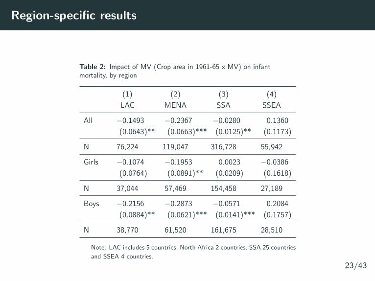
Table 2: Impact of MV (Crop area in 1961-65 x MV) on infantmortality, by region

(1) (2) (3) (4)

LAC MENA SSA SSEA

All −0.1493 −0.2367 −0.0280 0.1360

(0.0643)** (0.0663)*** (0.0125)** (0.1173)

N 76,224 119,047 316,728 55,942

Girls −0.1074 −0.1953 0.0023 −0.0386

(0.0764) (0.0891)** (0.0209) (0.1618)

N 37,044 57,469 154,458 27,189

Boys −0.2156 −0.2873 −0.0571 0.2084

(0.0884)** (0.0621)*** (0.0141)*** (0.1757)

N 38,770 61,520 161,675 28,510

Note: LAC includes 5 countries, North Africa 2 countries, SSA 25 countries

and SSEA 4 countries.

23/43

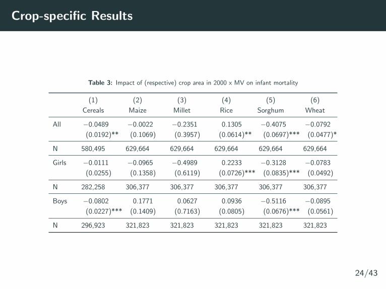
Crop-specific Results

Table 3: Impact of (respective) crop area in 2000 x MV on infant mortality

(1) (2) (3) (4) (5) (6)

Cereals Maize Millet Rice Sorghum Wheat

All −0.0489 −0.0022 −0.2351 0.1305 −0.4075 −0.0792

(0.0192)** (0.1069) (0.3957) (0.0614)** (0.0697)*** (0.0477)*

N 580,495 629,664 629,664 629,664 629,664 629,664

Girls −0.0111 −0.0965 −0.4989 0.2233 −0.3128 −0.0783

(0.0255) (0.1358) (0.6119) (0.0726)*** (0.0835)*** (0.0492)

N 282,258 306,377 306,377 306,377 306,377 306,377

Boys −0.0802 0.1771 0.0627 0.0936 −0.5116 −0.0895

(0.0227)*** (0.1409) (0.7163) (0.0805) (0.0676)*** (0.0561)

N 296,923 321,823 321,823 321,823 321,823 321,823

24/43

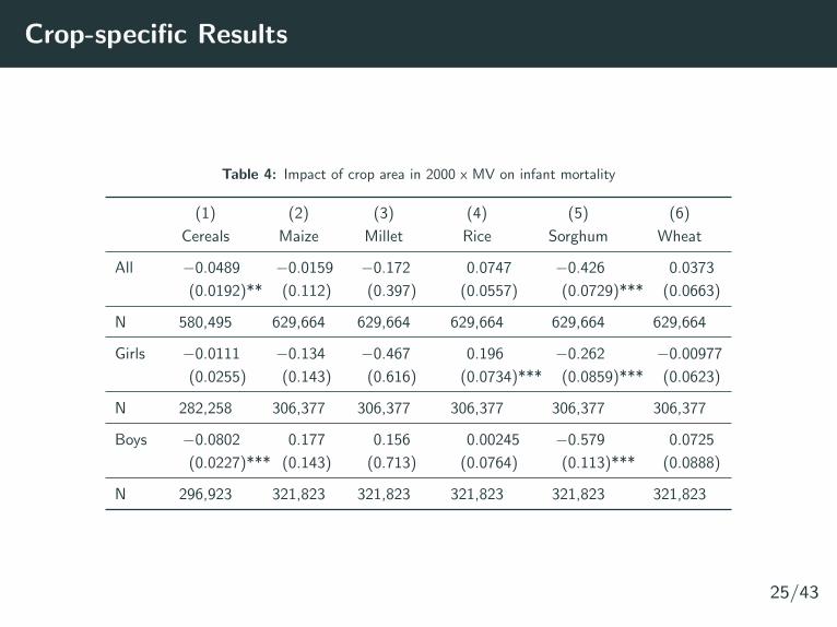
Crop-specific Results

Table 4: Impact of crop area in 2000 x MV on infant mortality

(1) (2) (3) (4) (5) (6)

Cereals Maize Millet Rice Sorghum Wheat

All −0.0489 −0.0159 −0.172 0.0747 −0.426 0.0373

(0.0192)** (0.112) (0.397) (0.0557) (0.0729)*** (0.0663)

N 580,495 629,664 629,664 629,664 629,664 629,664

Girls −0.0111 −0.134 −0.467 0.196 −0.262 −0.00977

(0.0255) (0.143) (0.616) (0.0734)*** (0.0859)*** (0.0623)

N 282,258 306,377 306,377 306,377 306,377 306,377

Boys −0.0802 0.177 0.156 0.00245 −0.579 0.0725

(0.0227)*** (0.143) (0.713) (0.0764) (0.113)*** (0.0888)

N 296,923 321,823 321,823 321,823 321,823 321,823

25/43

Summary so far

• We use rich subnational data to study the differential impact

of MVs on infant mortality of boys and girls in 36 developing

countries

• Preliminary results suggests that a 25 percentage point

expansion of area planted to MVs is associated with a decline

of 1.2-1.5 percentage points in infant mortality

• Robust to weighted average of cereal (5 crop) areas in 2000 ×MV

• Robust to several tests, and across regions (except Asia)

26/43

Additional Analysis (in progress)

• Next steps:

• Mother fixed effects

• Improve inference by using data on timing of releases (DIIVA)

for “less endogenous” temporal variation

• Improve inference by using agro-ecological (GAEZ) suitability

for exogenous spatial variation in crop choice

• Improve inference by using agro-ecological (GAEZ) suitability

for exogenous spatial variation in MV

• Country case study

27/43

Using DIIVA in SSA - Preview of Status of Results

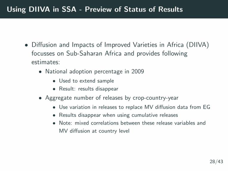
• Diffusion and Impacts of Improved Varieties in Africa (DIIVA)focusses on Sub-Saharan Africa and provides followingestimates:

• National adoption percentage in 2009

• Used to extend sample

• Result: results disappear

• Aggregate number of releases by crop-country-year

• Use variation in releases to replace MV diffusion data from EG

• Results disappear when using cumulative releases

• Note: mixed correlations between these release variables and

MV diffusion at country level

28/43

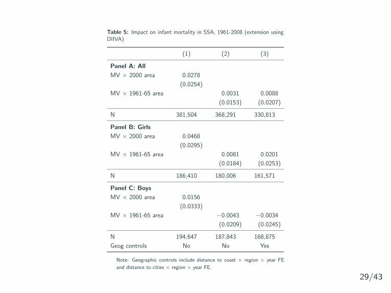
Table 5: Impact on infant mortality in SSA, 1961-2008 (extension usingDIIVA)

(1) (2) (3)

Panel A: All

MV × 2000 area 0.0278

(0.0254)

MV × 1961-65 area 0.0031 0.0088

(0.0153) (0.0207)

N 381,504 368,291 330,813

Panel B: Girls

MV × 2000 area 0.0468

(0.0295)

MV × 1961-65 area 0.0081 0.0201

(0.0184) (0.0253)

N 186,410 180,006 161,571

Panel C: Boys

MV × 2000 area 0.0156

(0.0333)

MV × 1961-65 area −0.0043 −0.0034

(0.0209) (0.0245)

N 194,647 187,843 168,875

Geog controls No No Yes

Note: Geographic controls include distance to coast × region × year FE

and distance to cities × region × year FE.

29/43

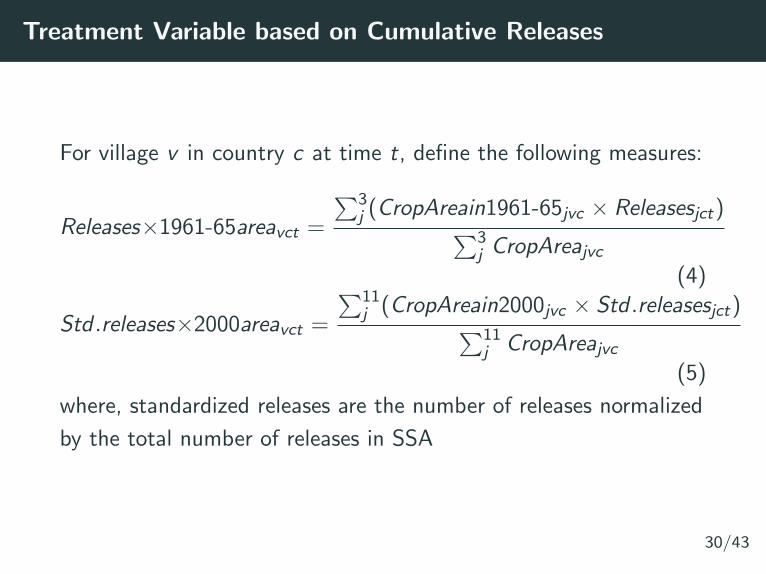
Treatment Variable based on Cumulative Releases

For village v in country c at time t, define the following measures:

Releases×1961-65areavct =

∑3j (CropAreain1961-65jvc × Releasesjct)∑3

j CropAreajvc(4)

Std .releases×2000areavct =

∑11j (CropAreain2000jvc × Std .releasesjct)∑11

j CropAreajvc(5)

where, standardized releases are the number of releases normalized

by the total number of releases in SSA

30/43

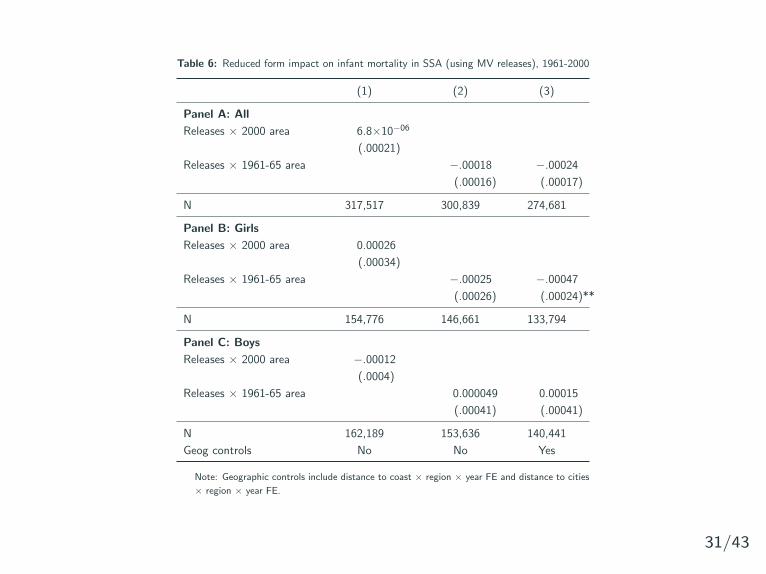
Table 6: Reduced form impact on infant mortality in SSA (using MV releases), 1961-2000

(1) (2) (3)

Panel A: All

Releases × 2000 area 6.8×10−06

(.00021)

Releases × 1961-65 area −.00018 −.00024

(.00016) (.00017)

N 317,517 300,839 274,681

Panel B: Girls

Releases × 2000 area 0.00026

(.00034)

Releases × 1961-65 area −.00025 −.00047

(.00026) (.00024)**

N 154,776 146,661 133,794

Panel C: Boys

Releases × 2000 area −.00012

(.0004)

Releases × 1961-65 area 0.000049 0.00015

(.00041) (.00041)

N 162,189 153,636 140,441

Geog controls No No Yes

Note: Geographic controls include distance to coast × region × year FE and distance to cities

× region × year FE.

31/43

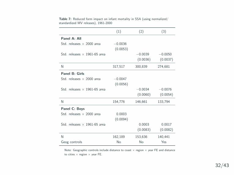
Table 7: Reduced form impact on infant mortality in SSA (using normalized/standardized MV releases), 1961-2000

(1) (2) (3)

Panel A: All

Std. releases × 2000 area −0.0036

(0.0053)

Std. releases × 1961-65 area −0.0039 −0.0050

(0.0036) (0.0037)

N 317,517 300,839 274,681

Panel B: Girls

Std. releases × 2000 area −0.0047

(0.0056)

Std. releases × 1961-65 area −0.0034 −0.0076

(0.0060) (0.0054)

N 154,776 146,661 133,794

Panel C: Boys

Std. releases × 2000 area 0.0003

(0.0094)

Std. releases × 1961-65 area 0.0003 0.0017

(0.0083) (0.0082)

N 162,189 153,636 140,441

Geog controls No No Yes

Note: Geographic controls include distance to coast × region × year FE and distance

to cities × region × year FE.

32/43

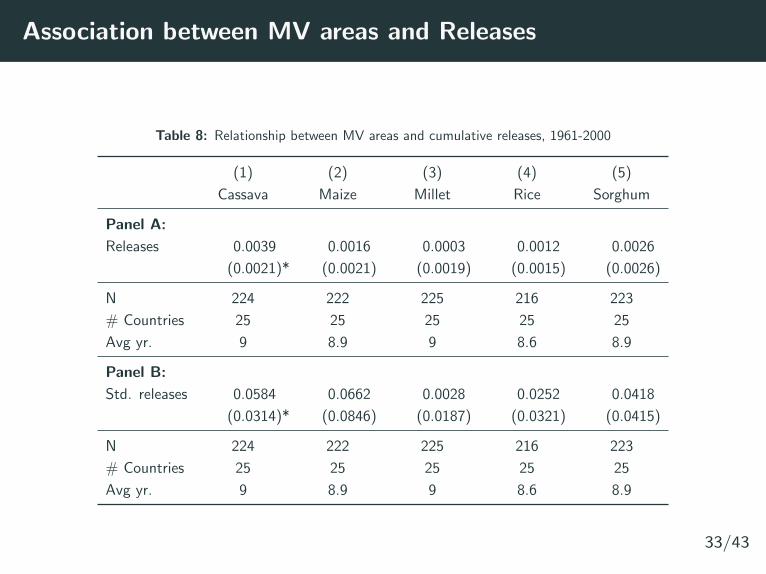
Association between MV areas and Releases

Table 8: Relationship between MV areas and cumulative releases, 1961-2000

(1) (2) (3) (4) (5)

Cassava Maize Millet Rice Sorghum

Panel A:

Releases 0.0039 0.0016 0.0003 0.0012 0.0026

(0.0021)* (0.0021) (0.0019) (0.0015) (0.0026)

N 224 222 225 216 223

# Countries 25 25 25 25 25

Avg yr. 9 8.9 9 8.6 8.9

Panel B:

Std. releases 0.0584 0.0662 0.0028 0.0252 0.0418

(0.0314)* (0.0846) (0.0187) (0.0321) (0.0415)

N 224 222 225 216 223

# Countries 25 25 25 25 25

Avg yr. 9 8.9 9 8.6 8.9

33/43

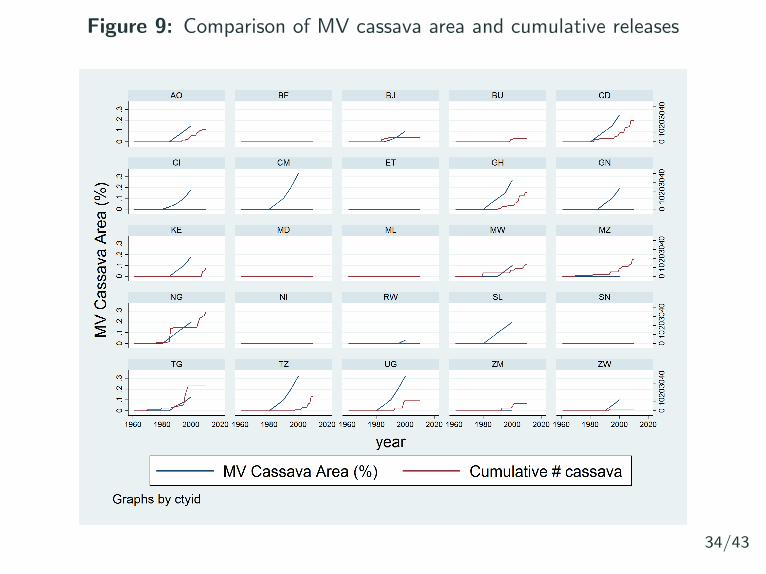
Figure 9: Comparison of MV cassava area and cumulative releases

34/43

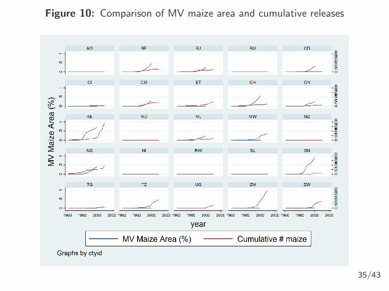
Figure 10: Comparison of MV maize area and cumulative releases

35/43

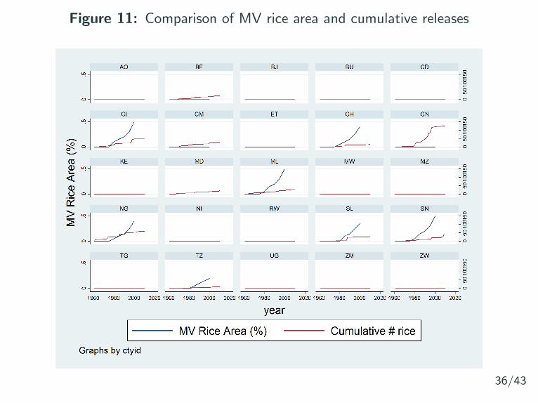
Figure 11: Comparison of MV rice area and cumulative releases

36/43

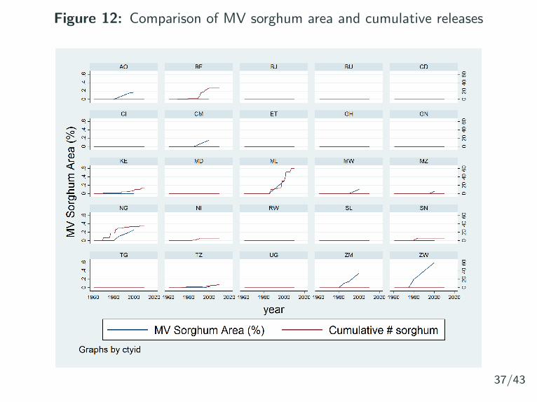
Figure 12: Comparison of MV sorghum area and cumulative releases

37/43

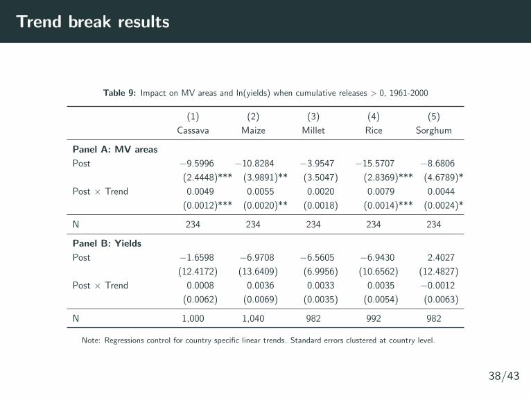
Trend break results

Table 9: Impact on MV areas and ln(yields) when cumulative releases > 0, 1961-2000

(1) (2) (3) (4) (5)

Cassava Maize Millet Rice Sorghum

Panel A: MV areas

Post −9.5996 −10.8284 −3.9547 −15.5707 −8.6806

(2.4448)*** (3.9891)** (3.5047) (2.8369)*** (4.6789)*

Post × Trend 0.0049 0.0055 0.0020 0.0079 0.0044

(0.0012)*** (0.0020)** (0.0018) (0.0014)*** (0.0024)*

N 234 234 234 234 234

Panel B: Yields

Post −1.6598 −6.9708 −6.5605 −6.9430 2.4027

(12.4172) (13.6409) (6.9956) (10.6562) (12.4827)

Post × Trend 0.0008 0.0036 0.0033 0.0035 −0.0012

(0.0062) (0.0069) (0.0035) (0.0054) (0.0063)

N 1,000 1,040 982 992 982

Note: Regressions control for country specific linear trends. Standard errors clustered at country level.

38/43

Global Agro-Ecological Zones

• Food and Agriculture Organization of the United Nations

(FAO) and the International Institute for Applied Systems

Analysis (IIASA) have developed an Agro-Ecological Zones

(AEZ) methodology to assess agricultural resources and

potential

• GAEZ provides data on agricultural suitability and potentialyields for:

• four input levels (high, intermediate, low and mixed)

• five water supply system types (rain-fed, rain-fed with water

conservation, gravity irrigation, sprinkler irrigation and drip

irrigation)

• at crop level (49 crops)

• for baseline climate (1961-1990) and future climate conditions

39/43

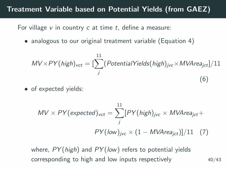
Treatment Variable based on Potential Yields (from GAEZ)

For village v in country c at time t, define a measure:

• analogous to our original treatment variable (Equation 4)

MV×PY (high)vct = [11∑j

(PotentialYields(high)jvc×MVAreajct ]/11

(6)

• of expected yields:

MV × PY (expected)vct =11∑j

[PY (high)jvc ×MVAreajct+

PY (low)jvc × (1−MVAreajct)]/11 (7)

where, PY (high) and PY (low) refers to potential yields

corresponding to high and low inputs respectively 40/43

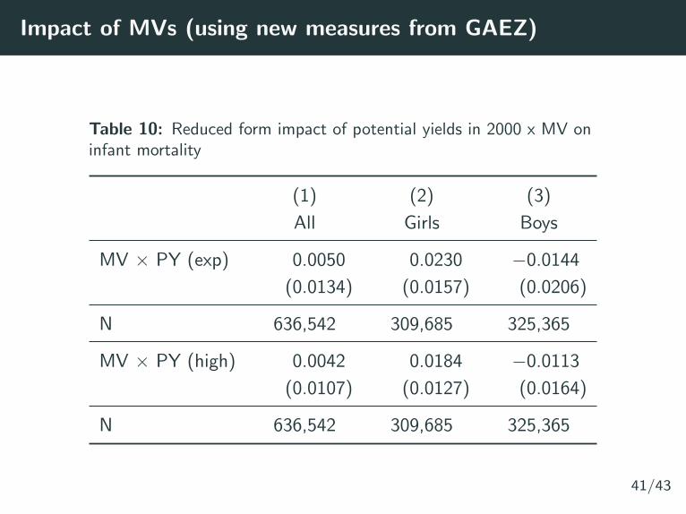
Impact of MVs (using new measures from GAEZ)

Table 10: Reduced form impact of potential yields in 2000 x MV oninfant mortality

(1) (2) (3)

All Girls Boys

MV × PY (exp) 0.0050 0.0230 −0.0144

(0.0134) (0.0157) (0.0206)

N 636,542 309,685 325,365

MV × PY (high) 0.0042 0.0184 −0.0113

(0.0107) (0.0127) (0.0164)

N 636,542 309,685 325,365

41/43

Country Case Study Options

• India: Data is available on district (admin level 2) level data

on wide range of agricultural indicators from 1966 to 2009.

DHS type data is not geo-referenced but potentially available

at similar resolution.

• Ethiopia: compiled subnational data (admin level 1) on input

use (MVs, irrigation, fertilizers and pesticides) from 1997 to

2010 (at 10 points of time) and plan to link it to LSMS-ISA

and DHS

• Other suggestions?

42/43

References

Evenson, R. E. and Gollin, D. (2003). Crop variety improvement and its effect on

productivity: The impact of international agricultural research. CABI.

Monfreda, C., Ramankutty, N., and Foley, J. A. (2008). Farming the planet: 2.

geographic distribution of crop areas, yields, physiological types, and net primary

production in the year 2000. Global biogeochemical cycles, 22(1).

Ray, D. K., Ramankutty, N., Mueller, N. D., West, P. C., and Foley, J. A. (2012).

Recent patterns of crop yield growth and stagnation. Nature communications,

3:1293.

43/43