Subjective Well-Being: Keeping up with the Joneses.

Real or Perceived?

INCOMPLETE AND PRELIMINARY DRAFT

Cahit Guven ∗

University of Houston

Bent E. Sørensen †

University of Houston and CEPR

July 2007

Abstract

Using data from the General Social Survey, we study the role of income in self-reportedhappiness. Unexpected income gains increase happiness. Relative income is more importantthan absolute income, in particular, income relative to individuals’ own cohort working in thesame occupation group, and living in the same region. Perceptions about relative income aremore important than actual relative income in explaining individual well-being. Perceptionsabout one’s own social class is more important than the actual social class in explaininghappiness. Social standing and occupational prestige of the spouse increases individualwell-being but father’s social standing and occupational prestige during childhood decreasescurrent well-being. Watching TV is associated with lower levels of well-being but readingnewspapers is associated with higher levels of well-being. Perceptions play a higher role inexplaining happiness for those who watch TV more but newspaper readership decreases theimportance of perceptions in explaining happiness. The results are robust to instrumentingown income with sector level wages or compensation and instrumenting current perceivedrelative income with perceived relative income at 16 years old.

JEL Classification: D14, D63, I31,Keywords: income shock, relative income, perceptions, media.

∗Department of Economics, University of Houston, TX, 77204 e-mail: cguven@mail.uh.edu, tel:713 7433818†Department of Economics, University of Houston, TX, 77204, e-mail: bent.sorensen@mail.uh.edu, tel: 713

7433841, fax: 713 7433798. The authors thank to International Conference on Policies for Happiness in Siena,76th Annual SEA Meetings, 11th Texas Econometrics Camp, 7th Annual Missouri Economics Conference partic-ipants, and seminar participants at Sam Houston State University and University of Houston for their valuablecomments and suggestions.

1 Introduction

“Happiness is not achieved by the conscious pursuit of happiness; it is generally the by-product

of other activities.” Aldous Leonard Huxley (July 26, 1894 - November 22 1963) British philoso-

pher

“The pursuit of happiness” is called upon in the American Declaration of Independence

and the Kingdom of Bhutan explicitly endeavors to maximize “Gross National Happiness.”

Nonetheless, the economics profession has been wary of attempts to use measures of happiness

in spite of the ubiquitous use of “utility” functions. We follow the convention of reserving the

term “utility” for describing individuals choices between economic variables. However, self-

reported well-being is related to “utility” in the sense that well-being helps predict individuals

economic choices; see the survey by Bruno S. Frey and Alois Stutzer (2002).

In this paper, we study self-reported happiness which we also refer to as “subjective well-

being.” We employ data from the U.S. General Social Survey which is a panel of about 3000

individuals from 1970 to 2002. The Survey provides self-reported measures of well-being, such

as responses to questions about how happy and satisfied individual respondents are with their

lives.

We show that income fluctuations matter for individual well-being. Because individual in-

come may be endogenous, we verify that unexpected increases in the output or, more precisely,

sectoral Gross Domestic Product (GDP) of the sector which the individual is working increases

individual happiness. Moreover, we show that relative income is much more important than ab-

solute income in explaining individual well-being. In particular, income relative to individuals’

own cohort working in the same occupation group and living in the same region.

We then attack the unexplored issue of whether actual relative income matters for well-being

or whether it is the perception of relative income. If individuals envy the cars and houses of the

Joneses (the relevant comparison group), then actual relative income must the relevant variable.

On the other hand, if people simply care about their relative income then what must matter

is what they think the Joneses make. In General Social Survey, unlike any other survey data,

individuals are asked their opinion about their income relative to an average American family.

1

We show that perceptions about relative income are more important than actual relative income

in explaining happiness. Perceptions about one’s own social class is also more important than

the actual social class in explaining happiness. Social standing and occupational prestige of

the spouse increases individual well-being but father’s social standing and occupational prestige

during childhood decreases current well-being. Watching TV is associated with lower levels of

well-being but reading newspapers is associated with higher levels of well-being. Perceptions play

a higher role in explaining happiness for those who watch TV more but newspaper readership

decreases the importance of perceptions in explaining happiness. We also find that perceptions

about relative income are more important for females than males and perceptions play a much

important role for middle income group than low and high income group. Also, actual income

is not important for the happiness of middle income individuals.

Section 2 gives an overview of the economic literature on well-being. Section 3 discusses

the data and the construction of the variables used in the paper. Section 4 presents the basic

framework and estimation strategy while Section 5 presents the empirical findings of the paper.

Section 6 concludes. An appendix gives more detailed information about the U.S. General Social

Survey and the variables used in the paper.

2 Literature Review

Research on the concept and measurement of happiness has made great progress in psychology

since the 1950s. While there is virtually no direct connection between psychology and theoretical

economics. The high level of rigor typical for experimental psychology have helped to make the

new idea of measurable happiness palatable to at least some economists. But it took considerable

time before an economist actually used happiness data in economics (Easterlin, 1974).

We can classify happiness research in to two: research about individual characteristics,

mainly income; and research about the impact of macroeconomic variables on happiness. Most

economists take it as a matter of course that higher income leads to higher happiness. And why

not? A higher income expands individuals and countries opportunity set; that is, more goods

and services can be consumed. Psychologists are more subtle in this respect. They are not so

confident that higher income always leads to more satisfaction. Tibor Scitovsky (1976), in his

2

book “The Joyless Economy: The Psychology of Human Satisfaction” argues that a high level of

wealth brings continuous comfort and thereby prevents the pleasure that results from incomplete

and intermittent satisfaction of desires. More recently, Robert Frank (1999) emphasizes that

ever-increasing income and consumption have nothing to do with happiness.

Many scholars have identified a striking and curious relationship. Per capita income in United

States has risen very dramatically in recent decades, but the proportion of people considering

themselves to be “very happy” has fallen over the same time period. The effects of income

on happiness can also be studied by comparing people with different incomes at a particular

point in time who live in the same country. At first sight, people with higher income have more

opportunities to achieve whatever they desire. They can buy more material goods and services

and have a higher status in society. Conversely the poor are unhappy. After all, if someone

does not like a high income and believes that poverty makes people happier, he or she is free

to dispose of his high income at no cost. Perhaps people are really seeking nonmaterial goals in

life such as fulfillment or the meaning of life and are disappointed when material things fail to

provide them (Dittmar, 1992). Happiness in this sense can not be achieved by material factors.

Many economists in the past have noted that individuals compare themselves to others

with respect to income, consumption, status, or utility. In other words, relative income may

matter more than actual income; see the survey by Clark, Frijters and Shields 2007. One of

the earliest researchers to voice this opinion was Thorstein Veblen (1899). He coined the term

conspicuous consumption to describe the desire to impress other people. The relative income

hypothesis has been formulated and econometrically tested by James Duesenberry (1949), who

posits an asymmetric structure of externalities. People look upward when making comparisons

and wealthier people, therefore, impose a negative externality on poorer people but not vice

versa. As a result, savings rates depends on the percentile position in the income distribution

and not solely on the income level.

A major line of research has been begun by Bernard van Praag and Arie Kapteyn (1973).

They construct an econometrically estimated welfare function with a “preference shift” param-

eter that captures the tendency of material wants to increase as income increases. They find

that increases in income shift aspirations upward but that individual satisfaction nevertheless

increases. The preference shift destroys about 60 to 80 percent of the welfare effect of an in-

3

crease in income; that is, somewhat less than a third remains. On the other hand, high income

aspirations may also be formed through childhood. Winkelmann, Boes and Staub (2007) find

that there is a negative well-being externality of parental income on children’s current well-being

and children compare their actual income with the acquired aspiration level.

Fred Hirsch (1976) emphasizes the role of relative social status by calling attention to “po-

sitional goods.” For instance, only the rich will be able to afford servants. Robert Frank (1985)

argues that production of positional goods in the form of luxuries, such as exceedingly expensive

watches or yachts, is a waste of productive resources, as overall happiness is thereby decreased

rather than increased.

Social comparison theories say that people evaluate features of themselves or their lives by

comparing themselves with others. This was used to explain some otherwise puzzling aspects of

satisfaction research. However, attempts to confirm social comparison theory in real-life settings

have not always confirmed it. Examples of such studies are Diener and Fujita (1997) and Diener,

Diener and Diener (1995). Wright (1985) found that there was an effect of self-rated health on

satisfaction, but this was not affected by the comparison of others.

Gilbert and Trower (1990) argue that people choose their own targets for comparison. Dif-

ferent inferences can be made from comparisons. The choice of a comparison target is a flexible

process and is not determined solely by the proximity of accessibility of relevant others. There

may be two exceptions to this. One is academic academic achievement (Diener and Fujita,

1997). The second is industrial wages. In fact, people often make these comparisons; Ross

(1986) found that 89 percent of the people made comparisons with members of their immediate

circle for satisfaction at home, 82 percent for satisfaction at work, but only 61 percent did this

for satisfaction with life as a whole. Wills (1981) assembled findings which shows people can

both increase or decrease their well-being by comparison depending on their reference point.

Strack, Schwarz, Hippler and Deutsch (1985), Lyubomirsky and Ross (1997) confirm these find-

ings. Winkelmann and Schwarze (2005) argue that parents take into account the situation of

their children while evaluating their own situation. They find that one standard deviation move

in the child’s well-being has the same effect as a 45 percent move in household income.

There are a number of reasons why an interpretation based chiefly on “relativity” notions

seems plausible. First, a certain amount of empirical support have been developed for the

4

relative income concept in other economic applications, such as savings behavior and more

recently, fertility behavior, and labor force participation (Duesenberry, 1949; Easterlin, 1973,

1969; Freedman, 1963; Wachter, 1971). Second, similar notions such as “relative deprivation”

have gained growing theoretical acceptance and empirical support in sociology, political science,

and social psychology over the past several decades (Berkowitz, 1971; Davies, 1962; Gurr, 1970;

Homans, 1961; Merton, 1968; Pettigrew, 1967; Smelser, 1962; Stouffer 1949).

In a recent interesting article, Alberto Alesina, Rafael Di Tella, and Robert MacCulloch

(2001) find a large, negative, and significant effect of inequality on happiness in Europe, but

not in the U.S. According to the authors, there are two potential explanations for this. First,

Europeans prefer more equal societies. Second, social mobility is (or is perceived to be) higher

in the U.S., so being poor is not seen as affecting future incomes. They test these hypotheses

by partitioning the sample across income and ideological lines. There is evidence of “inequality

generated” unhappiness in the U.S. only for a sub-group of “rich leftists.” In Europe, inequality

makes the poor unhappy, as well as the “leftists.” This favors the hypothesis that inequality

affects European happiness because of their lower social mobility (since no preference for equality

exists amongst the rich or the right). Recently, Carol Graham (2004) argues that absolute income

levels matter up to a certain point—particularly when basic needs are not met but after that,

relative income differences matter more.

Economists mainly have been trying to understand the impact of macroeconomic variables

such as inflation, unemployment, growth on happiness. Oswald (1997) shows that happiness

with life appears to be increasing in the United States. The rise is small—it seems that extra

income is not contributing dramatically to the quality of peoples’ lives. Since the early 1970s,

reported levels of satisfaction with life in European countries have on average risen very slightly

and unemployed people are very unhappy. Reported happiness is high among married, high

income, women, whites, well-educated, self-employed, retired, and homemakers. Happiness is

apparently U-shaped in age. Oswald (1997) finds that what matters for happiness is individuals’

own income not relative income.

Economists have been also studying the relationship between individual characteristics and

happiness. In a recent article, Rainer Winkelmann (1998) investigates interdependencies at the

family level. He also demonstrates how to model and test for such interdependencies using

5

the framework of an ordered probit model with multiple random effects. There clearly are

important interdependencies in reported well-being among members of the same family, some of

which may have biological origins. These need to be reckoned with, if one wants to understand

the determinants of subjective well-being.

People of higher age may be less happy than young people. This idea may have been

strengthened by the “youth cult” projected by the media which suggests that many desirable

qualities of life lie with youth. In some regards, the elderly are indeed objectively worse off. They

tend to be in poorer health and have lower income, and fewer of them are still married. Somewhat

surprisingly, many studies have found that older people are subjectively more happy than are

young people, but this effect tends to be very small. There are four potential explanations

of the observed positive relationship between age and happiness: First, the elderly have lower

expectations and aspirations. Second, the gap between goals and achievement is lower. Third,

older individuals have had time to adjust to their conditions. Fourth, they learn how to reduce

negative life events and to regulate negative affects. The positive relationship between age

and happiness has, however, been challenged and contradictory findings have been reported

(Horley and Lavery, 1995). Economists have identified a U-shaped relationship between age and

happiness (Oswald 1997, Blanchflower and Oswald, 2000). For several reasons it is difficult to

capture the influence of age on well-being. The term happiness may change its meaning with

age. The age effect may interfere with a cohort effect. Even causation is not as clear as it seems

to be at first sight. Happy people live a little longer than unhappy people, which contribute to

a positive correlation between age and happiness. Because of these problems, much care should

be taken when claiming that age leads to unhappiness, or that the elderly are happier than the

young.

Race. Blacks tend to be less happy than whites in all psychological and sociological studies

in the United States. But it also hold for other countries such as South Africa, where whites,

followed are the happiest people followed by Indians, coloreds and blacks (Moller, 1989). The

reasons lower incomes, less education, and less skilled jobs for black people. If one control for

these factors, the difference in happiness between races become small. A major reason for the

lower subjective well-being of the blacks maybe lower self-esteem, which in turn is likely to be

caused by their lower status in society. Economists have found that American blacks are less

6

happy than whites (Blanchflower and Oswald, 2000)

When people are asked to evaluate the importance of various areas of their lives, good health

obtains the highest ratings. Happiness and health are highly correlated, but this only holds for

self-reported health ratings. This is partly due to self-reported happiness and self-reported health

both being influenced by personality. For example, neurotic persons recalled more symptoms of

bad health and they a lower level of happiness than non-neurotics (Larsen, 1992). The effect

of objective health on happiness is smaller. People seem to be remarkably effective in coping.

Thus, they compare themselves to people in worse health, which induces a more positive image

of their own health conditions.

To have an enduring, intimate relationship is a major goals for most people. To have friends,

companions, and relatives and to be part of a group, be it co-workers or fellow church members,

contribute to happiness. The importance of “belonging” is reflected by the experimental findings

that even trivial definitions of groups lead to group identification and affect the dividing up of

money (Tajfel, 1981). Marriage raises happiness, as has been found in a large number of studies

for different countries and periods. Married men and women report similar levels of subjective

well-being; that is, marriage does not benefit one gender more than other. These results go well

with the observation that marriage brings marked advantages in terms of mortality, morbidity,

and mental health (Lee, Seccombe and Shehan, 1991). Couples also positively affect each other’s

well-being. The positive relationship between marriage and happiness persists, even when the

influence of variables such as income, age, and education is controlled for. Does marriage cause

happiness or does happiness promote marriage? A selection effect cannot be ruled out. It seems

reasonable to say that dissatisfied and introverted people find it more difficult to find a partner.

It is possibly more fun to be with extroverted, trusting, and compassionate people. Happy and

confident people are more likely to marry and to stay married (Veenhoven, 1989). But research

has led to the conclusion that this selection effect is not strong and the positive association of

marriage and happiness is mainly due to the beneficial effects of marriage (Mastekaasa, 1995).

There are two reasons why marriage contributes to happiness: First, marriage provides addi-

tional source of self-esteem. Second, married people have a better chance to benefit from an

enduring and supportive intimate relationship, and they suffer less from loneliness. Economic

research on happiness has also found that marriage and happiness are positively correlated,

7

holding other influences constant. Second, third, and fourth marriages turn out to be less happy

than first marriages (Blanchflower and Oswald, 2000).

The level of education bears little relationship to happiness. Education may indirectly

contribute to happiness by allowing a better adaptation to changing environments. But it also

tends to raise aspiration levels. It has, for instance been found that highly educated are more

distressed than the less educated when they are hit by unemployment (Clark and Oswald, 1994).

The impact of media on individual well-being has not been investigated in the literature

in detail yet. Recently, Frey, Stutzer and Benesch (2007) have shown that heavy TV viewers

do not benefit, but instead report lower satisfaction levels when exposed to more TV channels.

However, this is counter to the idea that a larger choice set does not make people worse off.

Moreover, long TV hours are also linked to higher material aspirations and anxiety.

3 Data

The U.S. General Social Survey includes an occupational classification of individuals and also a

sectoral classification. When the survey is done, every occupational category has been assigned

a NAICS level sectoral classification by the U.S. Census Bureau. We match individual data from

this survey with sectoral GDP data from the Bureau of Economic Analysis. Data are deflated

by the U.S. Consumer Price Index. Our dependent variable is the question “Taking everything

all together, how happy are you with the overall life.” In the U.S. General Social Survey, the

happiness data consists of categorical variables taking the values 1, 2, and 3 which in order refers

to “not too happy,” “pretty happy,” and “very happy” categories. Our dependent variable is the

happiness variable taking the values 1, 2, and 3. In order to have a binary variable, we redefine

the happiness variables as a binary variable where 1 (“more happy”) refers to “pretty happy”

and “very happy” categories and 0 refers to “not too happy” category.

In the U.S. General Social Survey, income is a categorical variable taking values 1–13 where 13

is the highest income level. In order to calculate relative income, we use the midpoint method.

Since, we know the lowest and highest income values in a category, we calculate individual

income as the midpoint income of their category. We calculate relative income by subtracting

own income from the reference point income. The reference point income is the average (within

8

the U.S. General Social Survey) income of an individual’s cohort who lives in the same region

and works in the same occupational group during the relevant year. Perceptions about relative

income are taken from the data as the answer to the question ‘What is your opinion about your

income relative to an average American.” This is a categorical variable taking the values 1-5

which in order refers to “far below average,” “below average,” “average,” “above average,” and

“far above the average.” Perceived social class variable is a categorical variable taking values

from 1-4 which is the answer to the question “If you were asked to one of four names for your

social class, which would you say you belong in? the lower class, the working class, the middle

class or the upper class?”. We use the occupational prestige scores and socio-economic index

created by the National Opinion Research. We use the number of hours in a day for TV watching.

Frequency of newspaper reading is a categorical variable taking values from 5-1, in order refers

to every day, a few times a week, once a week, less than once a week, or never.

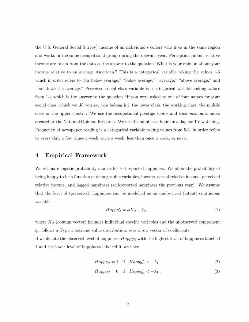
4 Empirical Framework

We estimate logistic probability models for self-reported happiness. We allow the probability of

being happy to be a function of demographic variables, income, actual relative income, perceived

relative income, and lagged happiness (self-reported happiness the previous year). We assume

that the level of (perceived) happiness can be modelled as an unobserved (latent) continuous

variable

Happy∗it = φXit + ξit , (1)

where Xit (column vector) includes individual specific variables and the unobserved component

ξit follows a Type 1 extreme value distribution. φ is a row vector of coefficients.

If we denote the observed level of happiness Happyit with the highest level of happiness labelled

1 and the lower level of happiness labelled 0, we have

Happyit = 1 if Happy∗it > −λ1 (2)

Happyit = 0 if Happy∗it < −λ1 , (3)

9

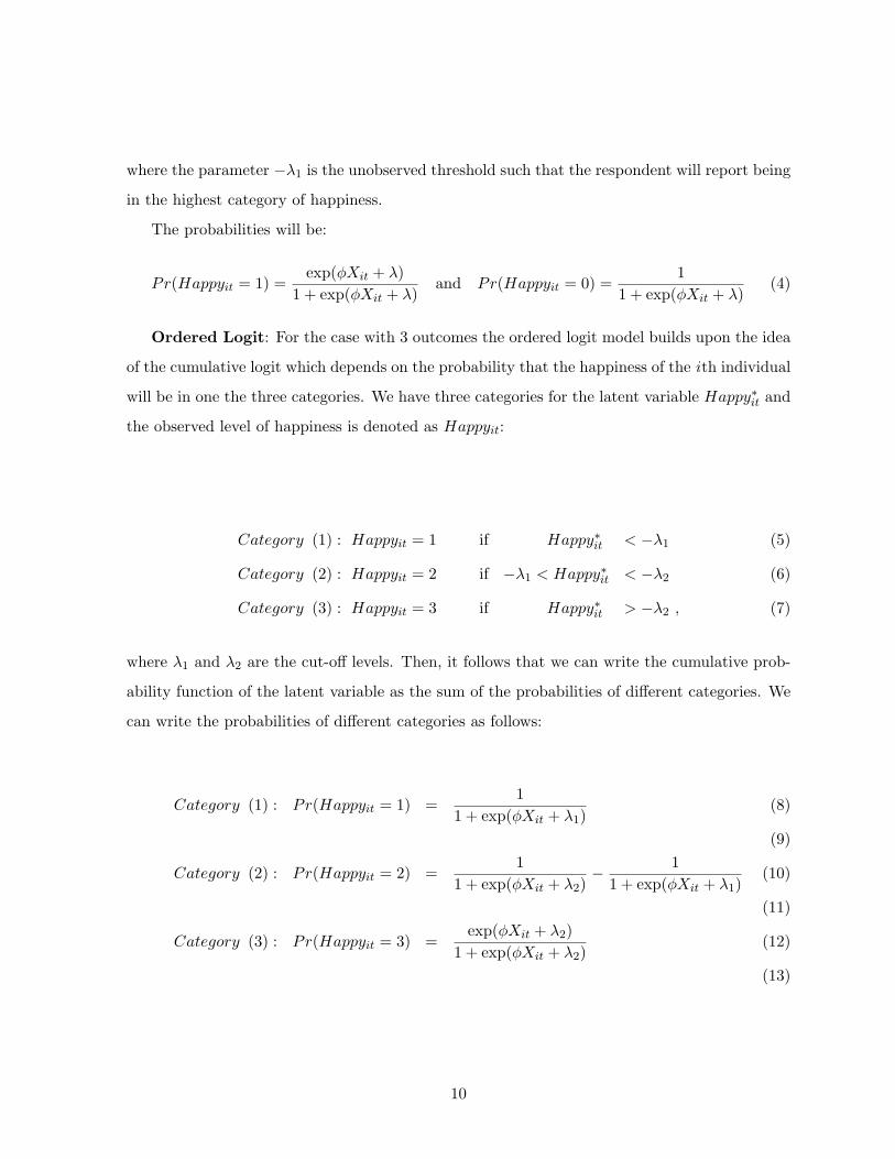
where the parameter −λ1 is the unobserved threshold such that the respondent will report being

in the highest category of happiness.

The probabilities will be:

Pr(Happyit = 1) =exp(φXit + λ)

1 + exp(φXit + λ)and Pr(Happyit = 0) =

11 + exp(φXit + λ)

(4)

Ordered Logit: For the case with 3 outcomes the ordered logit model builds upon the idea

of the cumulative logit which depends on the probability that the happiness of the ith individual

will be in one the three categories. We have three categories for the latent variable Happy∗it and

the observed level of happiness is denoted as Happyit:

Category (1) : Happyit = 1 if Happy∗it < −λ1 (5)

Category (2) : Happyit = 2 if −λ1 < Happy∗it < −λ2 (6)

Category (3) : Happyit = 3 if Happy∗it > −λ2 , (7)

where λ1 and λ2 are the cut-off levels. Then, it follows that we can write the cumulative prob-

ability function of the latent variable as the sum of the probabilities of different categories. We

can write the probabilities of different categories as follows:

Category (1) : Pr(Happyit = 1) =1

1 + exp(φXit + λ1)(8)

(9)

Category (2) : Pr(Happyit = 2) =1

1 + exp(φXit + λ2)− 1

1 + exp(φXit + λ1)(10)

(11)

Category (3) : Pr(Happyit = 3) =exp(φXit + λ2)

1 + exp(φXit + λ2)(12)

(13)

10

We can then turn the cumulative probability into the cumulative logit and we can write the

cumulative logit as a function of independent variables.

Marginal Probabilities: Since the coefficients from logit models for categorical variables

is not easily interpretable, we also report marginal probabilities. In this paper, the marginal

probability is defined as the effect on the predicted probability of being very happy of a one unit

decline in the mean of the relevant regressor calculated at the third outcome (“very happy”).

If -θ represents the marginal change in variable i (θ = 1 in this paper), the marginal probability

takes the form:exp(φ̂X̄ + λ̂2 − φk θ)

1 + exp(φ̂X̄ + λ̂2 − φk θ)− exp(φ̂X̄ + λ̂2)

1 + exp(φ̂X̄ + λ̂2), (14)

where φ̂i is the estimated coefficient to variable i and k is the independent variable of interest.

5 Empirical Results

Table 1 displays summary statistics, cross-tabulating indicators of work status with self-reported

happiness. We observe that retired individuals and home makers report the largest fraction of

very happy individuals although these groups also have somewhat higher numbers of less happy

individuals compared to full time employed. Unemployed people are the least happy in the

survey. Table 1 also shows the relationship between education and happiness. The education

categories are less than high school, high school, junior college, bachelor and graduate. When

we compare the education categories, we see that graduates are the happiest and and as the

degree of education decreases the happiest category decreases and less than high school is the

category displaying the least happiness. Marital and health status are also cross-tabulated with

happiness in Table 1. Married people are happier than others and widowed and single people are

pretty happy, while separated and divorced people represent the lowest category of happiness.

Health is strongly correlated with happiness. People who are healthiest are also happiest and

there is overall a strong correlation between happiness and health status.

Table 2 cross-tabulates perceived income rankings and happiness and we see a positive rela-

tionship between perception about relative income and happiness.

11

Table 3 cross-tabulates perceived social class rankings and happiness and we see a positive

relationship between perception about own’s social class compared to others and happiness.

Table 4 cross-tabulates newspaper readership rankings and happiness and we see a positive

relationship between reading newspaper and happiness.

Perceived relative income is, not surprisingly, closely related to actual relative income. Ta-

ble 5 shows that perceived income ranking and actual income ranking of individuals are positively

correlated but the correlation coefficient is clearly far from unity. This lack of perfect correlation

allows us to estimate the impact of perceived as well as actual income ranking simultaneously

and evaluate if both matters for happiness and which one is more important.

Table 6 reports the coefficients from the estimation of the ordered logit model and, for

interpretation, the increase in the marginal probability of being “very happy” for a unit decrease

in the corresponding right-hand side variable. We find that “high income” but not “middle

income” has a significant effect on happiness.

Consider employment status. The omitted category is the full time working category and we

see that individuals working part time have a probability of being in the “very happy” category

that is 1 percentage lower than that of individuals working full time. Unemployed individuals

are the least happy with a probability of being very happy that is 4.3 percentage points lower

than that of full time employed. The impact of being temporarily unemployed, student, or

homemaker is insignificant.

Marital status is a very strong predictor of happiness. For marital status the omitted category

is being married. Separated have a probability of being very happy that is 0.03 percentage points

lower than that of married individuals. Widowed, single, and divorced are even less likely to be

very happy. Regarding number of children in the family, the omitted category is having zero

or one child. The regression results show that people who have more than 2 children are more

likely to be very happy than individuals with 2 children, who are more likely to be very happy

than individuals with only one child. The probability of being very happy is U-shaped in age

with a minimum around 30 years of age.

We have five categories for education and the omitted category is the “less than high school”

category. We see that having a graduate degree significantly improves the probability of being

very happy. Considering gender, females are more likely to be “very happy” than males. Blacks

12

and other races are less happy than whites and blacks are the least happy category.

Health status is the single most important determinant of happiness. There are four cat-

egories of health with “poor health” the left-out category. Happiness is strongly increasing in

health and people with excellent health are much more likely to be happy than other people.

Last, Table 6 reports the impact of income on happiness and we recode the income variables

in to 3 categories. We find that people who earn more than the 25th percentile are significantly

happier than others. However, the direction of causality for these results are not necessarily

unidirectional from happiness to income.

Although we find that income and happiness are correlated, the direction of causality may go

in both directions. We, therefore, use sector specific income shocks as an exogenous determinant

of individual-level income, see Table 7. We find that, with ordered logit regression, income

shocks increase happiness when these are measured as exogenous sector level shocks. These

results suggest that following an unexpected increase in the output of a sector, people working

in this sector gains from this shock and become happier. 1

Tables 8 and 9 present the coefficients and marginal probabilities, respectively, for the impact

of relative income on happiness. We performed a series of regressions in order to identify the

reference group which had the strongest effect on happiness. We do not report the details but our

results indicate that individuals compare themselves to other individuals from their own cohort

who work in the same occupation and live in the same region. We report the results of regressions

using income relative to the reference group. We use the perceived relative income as a regressor

and examine if perceived income matters when actual relative income is also included. We use

the “real” values of absolute and relative income in all of the regressions. Winkelmann, Boes

and Lipp (2007) show that there is no money illusion with respect to individual satisfaction, that

is satisfaction depends on real rather than nominal income. This suggests that the perceived

income is “real” not “nominal”.

We find in Table 8,with ordered logit, which uses continuous variables as regressors that both

actual income and actual relative income are significant. However, perceived relative income is

the most significant regressor in absolute value. In Table 9 own actual income is very insignificant

1Winkelmann, Luechinger and Stutzer (2007) show that people have potential gains in well-being from workingin their job rather than in some alternative

13

and actual relative income is positive and significant while, again, perceived relative income has

a strong effect on happiness and is the most important regressor in absolute value.

Next, in Table 10, we investigate the importance of perceptions for males and females. We

find that, for males, income is clearly insignificant while actual relative income is marginally

significant at the 10 percent level. Perceived relative income is clearly significant. However,

this effect is larger and even more significant for females for whom we also find a significant

effect of own income. It appears that female well-being is more depending on income and, in

particular, perceived income status. Marital status has a bigger impact on happiness for females

and unemployment has a higher impact on happiness for women. Having two children relative to

fewer children makes males happier but does not effect females—maybe because they shoulder

a higher burden of child care.

Table 11 explores the fact that if we use actual and relative income as continuous variables

and perceptions about relative income as a categorical variable, again we find that own income

and actual income is insignificant but perceived relative income is highly significant.

Table 12 shows the impact of relative income and perceived relative income for different

income categories. We find that own income and lagged relative income are significant only

for high income category and relative income is significant only for the low income category.

Perceived relative income is significant for both low and middle income categories which implies

that perceptions about relative income does not play a role for the very rich.

Table 13 reports the results of instrumental variable probit regressions. We again recode

happiness as a binary variable. Low happiness category takes the value 0 while middle and

high happiness categories take the value 1. We instrument own income with average sector-level

wages and, alternatively, average sector-level compensation.2 Log own income instrumented by

sector level wage or compensation is insignificant and the IV-regressions confirm the result that

perceived relative income is more important than actual relative income.

Table 14 reports the results of instrumental variable probit regression. We again recode

happiness as a binary variable. Low happiness category takes the value 0 while middle and high

happiness categories take the value 1. We instrument perceived relative income with perceived

2We do not report that first-stage regressions in tables, but for sector level wage in the first stage, the estimatedcoefficient is 1.26 with a t-stat of 60.11 and an R-square of 0.55. The coefficient for compensation in the firststage is 1.43 with a t-statistic 70.04 and an R-square of 0.57.

14

relative income at 16 years old. 3 Log own income is insignificant , the relative income, and per-

ceived relative income are significant and again, IV-regressions confirm the result that perceived

relative income is more important than actual relative income.

In Table 15,Table16,Table 17 and Table 18 we use perceptions about social class, occupational

prestige, own income or socio-economic index as dependent variables. All of the correlations

among these dependent variables are less than 0.3. This lack of perfect correlation allows us

to estimate the impact of perceived as well as actual social class ranking simultaneously and

evaluate if both matters for happiness and which one is more important.

In Table 15, we investigate the role of perceptions about own’s own social class in explaining

current well-being. In the first column, we show that controlling own socio-economic situation,

perceptions about social class increases well-being. In the third column, we investigate the im-

pact of spouse’s socio-economic situation and the father’s socio-economic situation when the

individual was 16 years old. We find that spouse’s socio-economic situation increases well-being.

Probably this is because he/she adds to the household income and individual’s are proud of

his/her situation. On the other hand, as Winkelmann, Boes and Staub (2007) suggests, indi-

viduals may form higher aspirations during childhood because of their parent’s socio-economic

situation which leads to lower satisfaction.

Table 15 again shows the importance of perceived social class in explaining individual well-

being. However, we control for own income and occupational prestige in the first column. Again,

we find that perceptions play a very high role for happiness. The results in the second column,

also confirms the findings in Table 15. Spouses’s occupational prestige increases happiness but

father’s occupational prestige is correlated lower levels of well-being suggesting the idea of leading

to higher aspirations.

In Table 17 and Table 18, we look for possible determinants of “perception”. First, we

investigate the role of TV. People mostly see the richer, wealthier and more attractive people

on TV (Recently, CNN had a record of ratings during Paris Hilton’s interview after prison).

This may lead to wrong perceptions about relative income and also own social class. Secondly,

reading newspapers may have the same impact on people’s perceptions.

3We do not report that first-stage regressions in tables, but in the first stage, the estimated coefficient on theinstrument is is 0.1 with a t-stat of 17.49 and an R-square of 0.27

15

In Table 17, we find that again perceived relative income matters for well-being. TV watching

decreases happiness and also it enhances the impact of perceived relative income on happiness.

Perceptions matters more for heavy TV watchers. However, we find that newspaper readership

is associated with higher levels of well-being and moreover, it decreases the role of perceived

relative income in explaining happiness. Maybe this is because people who reads newspaper

have a better idea of other’s income. However, Putnam (1995) shows that access to mass media

(newspapers and TV) is positively correlated with measures of social capital.

In Table 18, we again investigate the role of media. We interact TV watching and newspaper

readership with perceived social class. We find that again, TV watching is associated with lower

level of happiness and it’s interaction with perceptions is nearly significantly positive suggesting

that perceptions about social class are more important for heavy TV watchers. Reading news-

papers increases well-being and it also decreases the role of perceptions suggesting people may

have a better idea of other’s socio-economic situation by reading newspapers.

6 Conclusion

To come

16

References

[1] Alesina, Alberto, Rafael Di Tella, Robert MacCulloch (2001), “Inequality and Happiness:

Are Europeans and Americans Different?” NBER Working Paper No. 8198.

[2] Andersen, Erling B. (1970), “Asymptotic Properties of Conditional Maximum Likelihood

Estimators, ” Journal of the Royal Statistical Society 32, pp. 283-301.

[3] Berkovitz, Leonard (1971), “Frustrations, Comparisons, and other Sources of Emotional

Arousal as Contributors to Social Unrest,” Journal of Social Issues 28, pp. 77-92.

[4] Blanchflower, David G., Andrew J. Oswald (2000), “Well-Being over Time in Britain and

the USA,” NBER Working Paper No. 7787.

[5] Blanchflower, David G., Andrew J. Oswald (2000), “The Rising Well-Being of the Young”

NBER Working Paper No. 6102.

[6] Blanchflower, David G., Richard B. Freeman (2000),“Youth Employment and Joblessness

in Advanced Countries,” Journal of Economic Literature 38, pp. 965-966.

[7] Chamberlain, Gary (1980), “Analysis of Covariance with Qualitative Data,” Review of

Economic Studies 47, pp. 225-238.

[8] Clark, Andrew, Andrew J. Oswald (1994), “Unhappiness and Unemployment,” Economic

Journal 104, pp. 648-659.

[9] Clark, Andrew, Paul Frijters, Micheal A. Shields (2007), “Relative Income, Happiness and

Utility: An Explanation for the Easterlin Paradox and Other Puzzles,” Journal of Economic

Literature forthcoming.

[10] Davies, James C. (1962), “Toward a Theory of Revolution,” American Sociological Review

27, pp. 5-19.

[11] Diener, Ed, Frank Fujita (1997), “Social Comparisons and Subjective Well-Being,” In B.

Buunk and F. X Gibbons (Ed.) Health, Coping, and Well-Being: Perspectives from Social

Comparison Theory pp. 329-357. Mahwah, New Jersey: Erlbaum.

17

[12] Diener, Ed, Marissa Diener, Carol Diener (1995), “ Factors Predicting the Subjective Well-

Being of Nations,” Journal of Personality and Social Psychology 69, pp. 851-864.

[13] Dittmar, Helga (1992), “The Social Psychology of Material Possessions,” Hemel Hamp-

stead: Harvester Wheatsheaf.

[14] Duesenberry, James S. (1949), “Income, Savings and the Theory of Consumer Behaviour,”

Cambridge, Mass: Harvard University Press.

[15] Easterlin, Richard A. (1969), “Towards a Socio-economic Theory of Fertility: A Survey

of Recent Research on Economic Factors in American Fertility,” in Samuel J. Behrman,

Leslie Corsa Jr., Ronald Freedman (Ed.) Fertility and Planning Family: a World View pp.

127-156. Ann Arbor: University of Michigan Press.

[16] Easterlin, Richard A. (1973), “Relative Economic Status and the American Fertility Swing,”

in Elenor B. Sheldon (Ed.), Familiy Economic Behavior: Problems and Prospects, Philadel-

phia: J. B. Lippincott for Institute of Life Insurance.

[17] Easterlin, Richard A. (1974), “Does Economic Growth Improve the Human Lot? Some

Empirical Evidence,” in Nations and Households in Economic Growth: Essays in Honour

of Moses Abramovitz, Paul A. David and Mel W. Reder (Ed.). New York and London:

Academic Press.

[18] Frank, Robert H. (1999), “Luxury Fever: Why Money Fails to Satisfy in an Era of Excess,”

New York: Free Press.

[19] Freedman, Deborah S. (1963), “The Relation of Economic Status on Fertility,” American

Economic Review 53, pp. 414-426.

[20] Frey, S. Bruno, Alois Stutzer, Christine Benesch (2007), “Does Watching TV Make Us

Happy?” Journal of Economic Psychology 28

[21] Frey, S. Bruno, Alois Stutzer (2002), “What Can Economists Learn from Happiness Re-

search,” Journal of Economic Literature 40, pp. 402-435.

18

[22] Gilbert, Paul, Trower, Peter (1990), “The Evolution and Manifestation of Social Anxiety”

In R. W. Crozier (Ed.), Shyness and Embarrassment: Perspectives from Social Psychology

pp. 144-177. New York: Cambridge University Press.

[23] Graham, Carol (2004), “Can Happiness Research Contribute to Development Economics?”

Washington DC: The Brookings Institution.

[24] Gurr, Ted R. (1970), “Why Men Rebel,” Princeton, New Jersey: Princeton University Press.

[25] Hirsch, Fred (1976), “The Social Limits to Growth,” Cambridge, Massachusetts: Harvard

University Press.

[26] Homans, Caspar George (1961), “Social Behavior: Its Elementary Forms,” American Soci-

ological Review 26, pp. 635-636.

[27] Horley, James, John J. Lavery (1995), “Subjective Well-Being and Age,” Social Indicator

Research 34, pp. 275-282.

[28] Larsen, Randy J. (1992), “Neuroticism and Selective Encoding and Recall of Symptoms:

Evidence from a Combined Concurrent-Retrospective Study,” Journal of Personality and

Social Psychology 62, pp. 480-488.

[29] Lee, Gary R., Auke Karen Seccombe, Constance L. Shehan (1991), “Marital Status and

Personal Happiness: An Analysis of Trend Data,” Journal of Marriage and the Family 53,

pp. 839-844.

[30] Lyubomirsky, Sonya, Lee Ross (1997), “Hedonic Consequences of Social Comparison: A

Contrast of Happy and Unhappy People,” Journal of Personality and Social Psychology 73,

pp. 1141-1157.

[31] Merton, Robert K. (1968), “Social Theory and Social Structure,” New York: Free Press.

[32] Mastekaasa, Arnel (1995), “Age Variations in the Suicide Rates and Self-Reported Subjec-

tive Well-Being of Married and Never Married Persons,” Journal of Community and Applied

Social Psychology 5, pp. 21-39.

[33] Moller, Valerie (1989), “Can’t Get no Satisfaction,” Indicator South Africa 7, pp. 43-46.

19

[34] Norbert Schwarz, Hans-J. Hippler, Brigitte Deutsch, Fritz Strack (1985), “Response Scales:

Effects of Category Range on Reported Behavior and Comparative Judgments,” Public

Opinion Quarterly 49, pp. 388-395.

[35] Oswald, J. Andrew (1997), “Happiness and Economic Performance,” Economic Journal

107, pp. 1815-1831.

[36] Pettrigrew, Thomas E. (1967), “Social Evaluation Theory: Convergences and Applications,”

Nebraska: University of Nebraska Press.

[37] Putnam, Robert (1995) “Bowling Alone: Americas Declining Social Capital,” Journal of

Democracy 6, pp. 65-78.

[38] Ross, D. Shachter (1986), “Evaluating Influence Diagrams,” Operations Research 34, pp.

871-882.

[39] Smelser, Neil J. (1962), “Theory of Collective Behavior,” New York: Free Press.

[40] Smolensky, Eugene (1965), “The Past and Present Poor: The Concept of Poverty,” Wash-

ington, DC: Chamber of Commerce of the United States.

[41] Scitovsky, Tibor (1976),“The Joyless Economy,” Oxford: Oxford University Press.

[42] Stouffer, Samuel A. (1949), “The American Soldier,” Princeton: Princeton University Press.

[43] Tajfel, Henri (1984), “Human Groups and Social Categories: Studies in Social Psychology,”

The American Journal of Sociology 90, pp. 209-211

[44] Van Praag, Bernard M. S., Arie Kapteyn (1973), “Wat Is Ons Inkomen Ons Waard?(How

Do We Value Our Income?)” Economisch Statistische Berichten 58, pp. 360-382.

[45] Veblen, Thorstein (1989), “The Theory of Leisure Class,” New York: The Modern Library.

[46] Veenhoven, Ruut (1989), “Does Happiness Bind? How Harmful Is Happiness?” Rotterdam:

Universitaire Pers Rotterdam.

[47] Wachter, Michael L. (1972), “A Labor Supply Model for Secondary Workers,” The Review

of Economics and Statistics 54, pp. 141-151.

20

[48] Wachter, Michael L. (1974), “A New Approach to the Equilibrium Labor Force,” Economica

41, pp. 35-51.

[49] Wills, Thomas A. (1981), “Downward Comparison Principles in Social Psychology,” Psy-

chological Bulletin 90, pp. 245-271.

[50] Winkellmann, Rainer, Simon Luechinger, Alois Stutzer (2007), “The Happiness Gains From

Sorting and Matching In The Labor Market,” University of Zurich Working Paper

[51] Winkellmann, Rainer, Stefan Boes, Markus Lipp (2007), “Money Illusion Under Test,”

Economics Letters 94, pp. 332-337.

[52] Winkellmann, Rainer, Stefan Boes, Kevin Staub (2007), “The Hidden Cost of Parental

Income:Why Less Maybe More,” University of Zurich Working Paper.

[53] Winkellmann, Rainer, Johannes Schwarze (2005), “What Can Happiness Research Tell Us

About Altruism? Evidence from the German Socio-Economic Panel,” University of Zurich

Working Paper.

[54] Winkelmann, Liliana, Winkellmann Rainer (1998), “Why Are the Unemployed So Un-

happy? Evidence from Panel Data,” Economica 65, pp. 1-15.

[55] Wright, Stephen C. (1985), “Health Satisfaction: A Detailed Test of the Multiple Discrep-

ancies Theory Model,” Social Indicators Research 17, pp. 299-313.

21

Data Appendix

The General Social Surveys have been conducted by the National Opinion Research Center

annually since 1972, except for the years 1979, 1981, and 1992 (a supplement was added in

1992), and biennially beginning in 1994. For each round of surveys, the Roper Center for Pub-

lic Opinion Research prepares a cumulative dataset that merges previous years of the General

Social Survey into a single file, with each year or survey constituting a subfile. The content of

each survey changes slightly as some items are added to or deleted from the interview schedule.

Main areas covered in the General Social Survey include socioeconomic status, social mobility,

social control, the family, race relations, sex relations, civil liberties, and morality. Topical mod-

ules designed to investigate new issues or to expand the coverage of an existing subject have

been part of the General Social Survey since 1977, when the first module on race, abortion,

and feminism appeared. The topical modules for 1998 focused on the themes of medical care,

medical ethics, religion, religion and health, culture, job experiences, and interracial friendships.

Other topics covered have included gender, emotions, market exchange, giving and volunteering,

and mental health (1996), family mobility and multiculturalism (1994), cultural issues (1993),

work organizations (1991), intergroup relations (1990), occupational prestige (1989), religious

socialization, behaviors, and beliefs (1988), sociopolitical participation (1987), the feminization

of poverty (1986), social networks (1985), and the role of the military (1982 and 1984). The

General Social Survey also added a crossnational component in 1985, through participation

in a multinational collaborative group called the International Social Survey Program (ISSP).

Topics addressed have included the role of government (1985, 1990, 1996, and 1998), social

support (1986), social inequality (1987), family and gender issues (1988 and 1994), work ori-

entation (1989 and 1998), the impact of religious background, behavior, and beliefs on social

and political preferences (1991 and 1998), environmental issues (1993), and national identity

(1996 and 1998). In 1994, two major innovations were introduced to the General Social Survey.

First, the traditional core set of questions was substantially reduced to allow for the creation

of mini-modules (small- to medium-sized supplements). The mini-modules permit greater flexi-

bility to incorporate innovations and to include important items proposed by the social science

community. Second, a new biennial, split-sample design was instituted, consisting of two paral-

lel subsamples of approximately 1,500 cases each. The two subsamples contain identical cores

22

and different topical ISSP modules. Regions are as follows. New England: Maine, Vermont,

New Hampshire, Massachusetts, Connecticut, Rhode Island. Middle Atlantic: New York, New

Jersey, Pennsylvania. East North Central: Wisconsin, Illinois, Indiana, Michigan, Ohio. West

North Central: Minnesota, Iowa, Missouri, North Dakota, South: Dakota, Nebraska, Kansas.

South Atlantic: Delaware, Maryland, West Virginia, Virginia, North Carolina, South Carolina,

Georgia, Florida, District of Columbia. East South Central: Kentucky, Tennessee, Alabama,

Mississippi. West South Central: Arkansas, Oklahoma, Louisiana, Texas. Mountain: Montana,

Idaho, Wyoming, Nevada, Utah, Colorado, Arizona, New Mexico. Pacific = Washington, Ore-

gon, California, Alaska, Hawaii.

VARIABLES USED IN THE PAPER:

Happiness: Happiness is the answer to the questions in U.S. General Social Survey “Taken

all together, how would you say things are these days-would you say you are very happy, pretty

happy or not too happy?” Happiness is a categorical variable where 1, 2, 3 in order refers to

the answers not too happy, pretty happy and happy. In the ordered logit regressions happiness

takes three values. However, because of the properties of fixed effects ordered logit regression

(explained in detail above), happiness is recoded as a binary variable.

Financial Satisfaction: Financial Satisfaction is the answer to the question in U.S General

Social Survey, “We are interested in how people are getting along financially these days. So far

as you and your family are concerned, would you say that you are pretty well satisfied with

your present financial situation, more or less satisfied, or not satisfied at all?” In the ordered

logit regressions financial satisfaction takes three values. However, because of the properties of

fixed effects ordered logit regression (explained in detail above), happiness is recoded as a binary

variable.

Actual income: This is the actual family income first coded as intervals in the dataset and

then computed with the midpoint method. Every individual is assigned to the average of the

lowest and highest income level of the interval they reported. We use the real family income

from the U.S General Social Survey which is corrected for CPI inflation. In the regressions we

use actual income as a continuous variable but since perceived relative income is a categorical

variable, we also recode the actual income in to 5 categories in order to make it comparable in

23

the regressions.

Actual relative income: Relative income is calculated as the difference of the actual in-

come and the average income of the reference point. We try different combinations of reference

groups with age, region, sector, occupation (one digit and three digit sectors and occupations).

The reference group we use in these paper is the individuals’cohort, working in the same occu-

pation group (one digit)and living in the same region (as explained above). In the regressions

we use actual relative income as a continuous variable but since perceived relative income is

a categorical variable, we also recode the actual income in to 5 categories in order to make it

comparable in the regressions.

Perceived Relative income: Perceived relative income is the answer to the question in the

U.S. General Social Survey, “Compared to an average American family, what is your opinion

about your family income.” This variable has 5 categories: Far below than average, below

average, average, above average, far above average. In the regressions we use perceived relative

income as a categorical variable but since actual relative income is a continuous variable, we

also use perceived relative income as a continuous variable taking values from 1 through 5 to

make it comparable in the regressions.

Perceived Relative Income When 16 yrs old: It is the answer to the question in the U.S.

GSS, “Thinking about the time when you were 16 years old, compared with American families in

general then, would you say your family income was far below average, below average, average,

above average, or far above average?” In the regressions we use perceived relative income when

16 yrs old as a categorical variable but since actual relative income is a continuous variable, we

also use it as a continuous variable taking values from 1 through 5 to make it comparable in the

regressions.

Lagged Relative Income: People know their own actual income this year but they may

not have information about others’income this year. They will just use the last period’s income

about others for their comparison. Lagged relative income is then the difference of current actual

income from the reference group income in the last period.

Health status: Excellent, good, fair and poor are the categories for health. Poor is the

omitted category in the regressions.

24

Marital Status: Married, widowed, divorced, separated and never married are the cate-

gories for marital status. Married is the omitted category in the regressions.

Work Status: Working full-time, working part-time, temporarily not working, unemployed,

retired, school, keeping house and others are the categories for work status. Working full-time

is the omitted category.

Sex: Male and Female are the categories. Male is the omitted category in the regressions.

Race: White, black, and others are the categories for race. White is the omitted category

in the regressions.

Education: We use number of years of schooling as a dependent variable and also use the

highest education as a categorical variable which has the values: less than high school, high

school, junior college, bachelor and graduate. Less than high school is the omitted category in

the regressions.

Children: We use the number of children as a dependent variable and also recode as a

categorical variables as having children less than 1, having 2 children and having children more

than 2. In the regressions, children less than 1 is the omitted category in the regressions.

Sectoral Wage: The variable is taken from Bureau of Economic Analysis. The monetary

remuneration of employees, including the compensation of corporate officers, commissions, tips,

and bonuses, voluntary employee contributions to certain deferred compensation plans, such as

401(k) plans, and receipts in kind that represent income. Accruals and disbursements differ in

the treatment of retroactive payments. In the national income and product accounts (NIPAs),

wage and salary accruals is the appropriate measure for gross domestic income (GDI) and wage

and salary disbursements is the appropriate measure for personal income.

Sectoral Compensation: The variable is taken from Bureau of Economic Analysis.

Income accruing to employees as remuneration for their work for domestic production. It is

the sum of wage and salary accruals and of supplements to wages and salaries. It includes

compensation paid to the rest of the world and excludes compensation received from the rest of

the world.

Occupational Prestige Score: The prestige scores assigned to occupations were taken

from rating systems developed at National Opinion Research Center (NORC) in in a project

on occupation prestige directed by Robert W. Hodge, Paul S. Siegel, and Peter H. Rossi. This

25

concept of prestige is defined as the respondents’ estimation of the social standing of occupa-

tions. The prestige scores in the Hodge-Siegel-Rossi and GSS studies were generated by asking

respondents to estimate the social standing of occupations via a nine-step ladder, printed on

cardboard and presented to the respondent.

Socio-Economic Index: Scores were originally calculated by Otis Dudley Duncan based

on NORC’s North-Hatt prestige study and the U.S. Census. Duncan regressed prestige scores

for 45 occupational titles on education and income to produce weights that would predict pres-

tige. This algorithm was then used to calculate socio-economic index scores for all occupational

categories employed in the Census classification of occupations. Similar procedures have been

used to produce socio-economic scores based on later NORC prestige studies and censuses.

Perceived Social Class: Answer to the question “If you were asked to one of four names

for your social class, which would you say you belong in? the lower class, the working class, the

middle class or the upper class?”

TV Hours: Answer from 0 to 24 to the question “On the average day, about how many

hours do you personally watch television?”

Newspaper: Categorical answer to the question “How often do you read the newspaper?”

every day, a few times a week, once a week, less than once a week, or never?

26

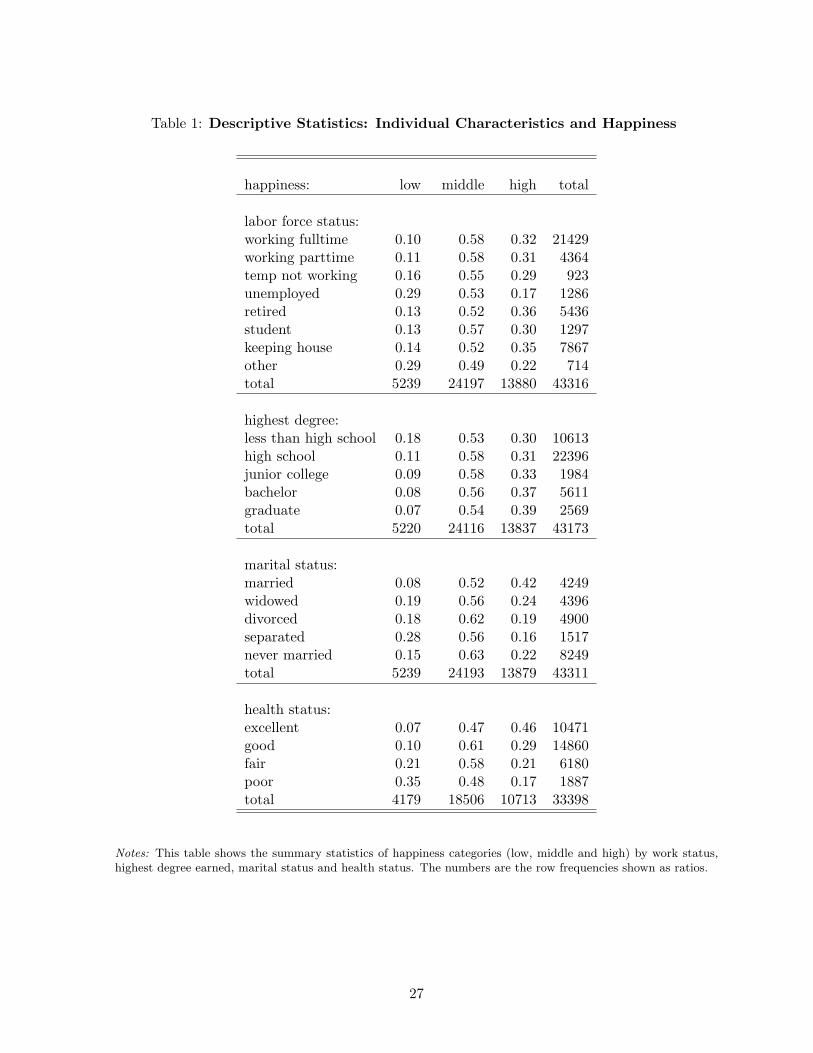
Table 1: Descriptive Statistics: Individual Characteristics and Happiness

happiness: low middle high total

labor force status:working fulltime 0.10 0.58 0.32 21429working parttime 0.11 0.58 0.31 4364temp not working 0.16 0.55 0.29 923unemployed 0.29 0.53 0.17 1286retired 0.13 0.52 0.36 5436student 0.13 0.57 0.30 1297keeping house 0.14 0.52 0.35 7867other 0.29 0.49 0.22 714total 5239 24197 13880 43316

highest degree:less than high school 0.18 0.53 0.30 10613high school 0.11 0.58 0.31 22396junior college 0.09 0.58 0.33 1984bachelor 0.08 0.56 0.37 5611graduate 0.07 0.54 0.39 2569total 5220 24116 13837 43173

marital status:married 0.08 0.52 0.42 4249widowed 0.19 0.56 0.24 4396divorced 0.18 0.62 0.19 4900separated 0.28 0.56 0.16 1517never married 0.15 0.63 0.22 8249total 5239 24193 13879 43311

health status:excellent 0.07 0.47 0.46 10471good 0.10 0.61 0.29 14860fair 0.21 0.58 0.21 6180poor 0.35 0.48 0.17 1887total 4179 18506 10713 33398

Notes: This table shows the summary statistics of happiness categories (low, middle and high) by work status,highest degree earned, marital status and health status. The numbers are the row frequencies shown as ratios.

27

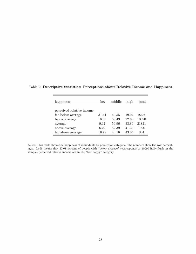
Table 2: Descriptive Statistics: Perceptions about Relative Income and Happiness

happiness: low middle high total

perceived relative income:far below average 31.41 49.55 19.04 2222below average 18.83 58.49 22.68 10090average 9.17 56.96 33.86 21821above average 6.22 52.39 41.39 7920far above average 10.79 46.16 43.05 834

Notes: This table shows the happiness of individuals by perception category. The numbers show the row percent-ages. 22.68 means that 22.68 percent of people with “below average” (corresponds to 10090 individuals in thesample) perceived relative income are in the “low happy” category.

28

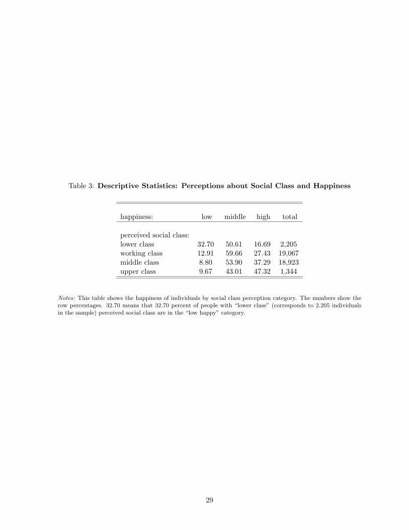
Table 3: Descriptive Statistics: Perceptions about Social Class and Happiness

happiness: low middle high total

perceived social class:lower class 32.70 50.61 16.69 2,205working class 12.91 59.66 27.43 19,067middle class 8.80 53.90 37.29 18,923upper class 9.67 43.01 47.32 1,344

Notes: This table shows the happiness of individuals by social class perception category. The numbers show therow percentages. 32.70 means that 32.70 percent of people with “lower class” (corresponds to 2.205 individualsin the sample) perceived social class are in the “low happy” category.

29

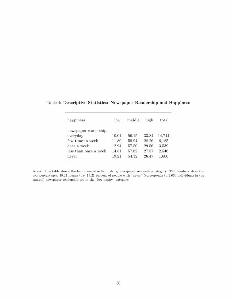
Table 4: Descriptive Statistics: Newspaper Readership and Happiness

happiness: low middle high total

newspaper readership:everyday 10.01 56.15 33.84 14,744few times a week 11.80 59.94 28.26 6,185once a week 12.94 57.50 29.56 3,539less than once a week 14.81 57.62 27.57 2,546never 19.21 54.32 26.47 1,666

Notes: This table shows the happiness of individuals by newspaper readership category. The numbers show therow percentages. 19.21 means that 19.21 percent of people with “never” (corresponds to 1.666 individuals in thesample) newspaper readership are in the “low happy” category.

30

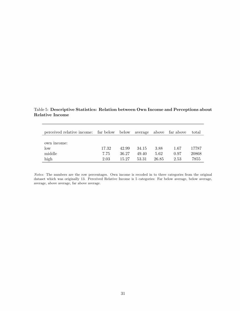
Table 5: Descriptive Statistics: Relation between Own Income and Perceptions aboutRelative Income

perceived relative income: far below below average above far above total

own income:low 17.32 42.99 34.15 3.88 1.67 17787middle 7.75 36.27 49.40 5.62 0.97 20868high 2.03 15.27 53.31 26.85 2.53 7855

Notes: The numbers are the row percentages. Own income is recoded in to three categories from the originaldataset which was originally 13. Perceived Relative Income is 5 categories: Far below average, below average,average, above average, far above average.

31

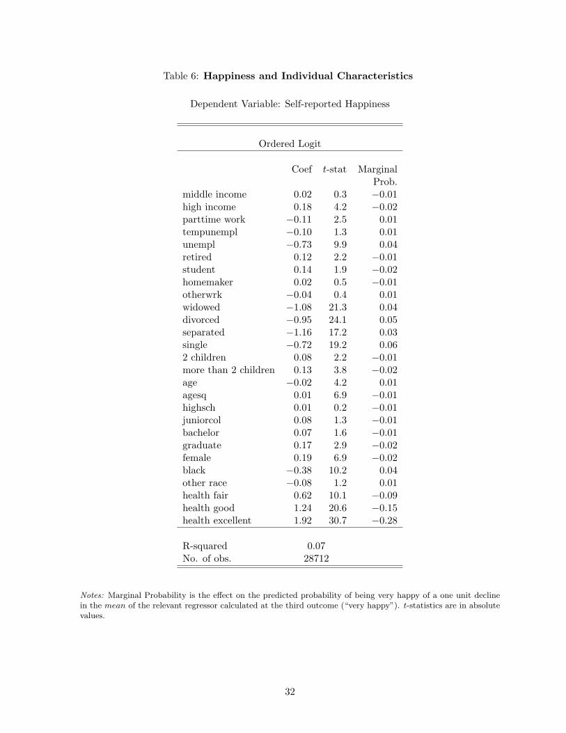
Table 6: Happiness and Individual Characteristics

Dependent Variable: Self-reported Happiness

Ordered Logit

Coef t-stat MarginalProb.

middle income 0.02 0.3 −0.01high income 0.18 4.2 −0.02parttime work −0.11 2.5 0.01tempunempl −0.10 1.3 0.01unempl −0.73 9.9 0.04retired 0.12 2.2 −0.01student 0.14 1.9 −0.02homemaker 0.02 0.5 −0.01otherwrk −0.04 0.4 0.01widowed −1.08 21.3 0.04divorced −0.95 24.1 0.05separated −1.16 17.2 0.03single −0.72 19.2 0.062 children 0.08 2.2 −0.01more than 2 children 0.13 3.8 −0.02age −0.02 4.2 0.01agesq 0.01 6.9 −0.01highsch 0.01 0.2 −0.01juniorcol 0.08 1.3 −0.01bachelor 0.07 1.6 −0.01graduate 0.17 2.9 −0.02female 0.19 6.9 −0.02black −0.38 10.2 0.04other race −0.08 1.2 0.01health fair 0.62 10.1 −0.09health good 1.24 20.6 −0.15health excellent 1.92 30.7 −0.28

R-squared 0.07No. of obs. 28712

Notes: Marginal Probability is the effect on the predicted probability of being very happy of a one unit declinein the mean of the relevant regressor calculated at the third outcome (“very happy”). t-statistics are in absolutevalues.

32

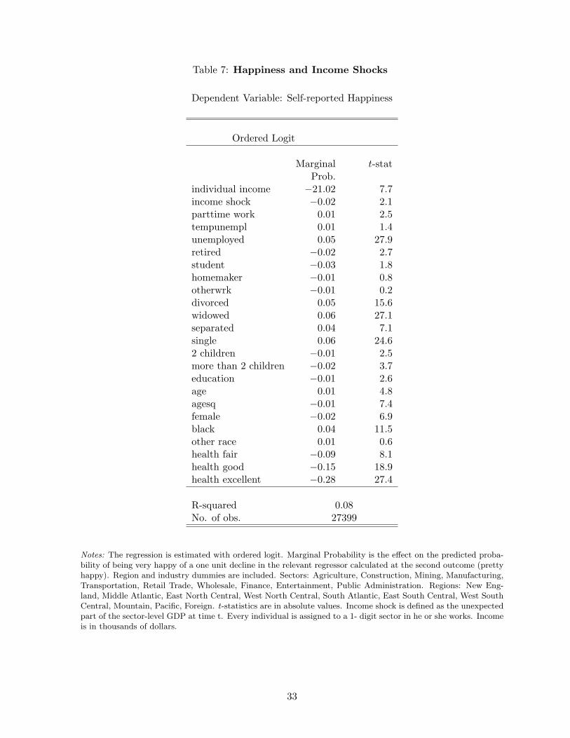
Table 7: Happiness and Income Shocks

Dependent Variable: Self-reported Happiness

Ordered Logit

Marginal t-statProb.

individual income −21.02 7.7income shock −0.02 2.1parttime work 0.01 2.5tempunempl 0.01 1.4unemployed 0.05 27.9retired −0.02 2.7student −0.03 1.8homemaker −0.01 0.8otherwrk −0.01 0.2divorced 0.05 15.6widowed 0.06 27.1separated 0.04 7.1single 0.06 24.62 children −0.01 2.5more than 2 children −0.02 3.7education −0.01 2.6age 0.01 4.8agesq −0.01 7.4female −0.02 6.9black 0.04 11.5other race 0.01 0.6health fair −0.09 8.1health good −0.15 18.9health excellent −0.28 27.4

R-squared 0.08No. of obs. 27399

Notes: The regression is estimated with ordered logit. Marginal Probability is the effect on the predicted proba-bility of being very happy of a one unit decline in the relevant regressor calculated at the second outcome (prettyhappy). Region and industry dummies are included. Sectors: Agriculture, Construction, Mining, Manufacturing,Transportation, Retail Trade, Wholesale, Finance, Entertainment, Public Administration. Regions: New Eng-land, Middle Atlantic, East North Central, West North Central, South Atlantic, East South Central, West SouthCentral, Mountain, Pacific, Foreign. t-statistics are in absolute values. Income shock is defined as the unexpectedpart of the sector-level GDP at time t. Every individual is assigned to a 1- digit sector in he or she works. Incomeis in thousands of dollars.

33

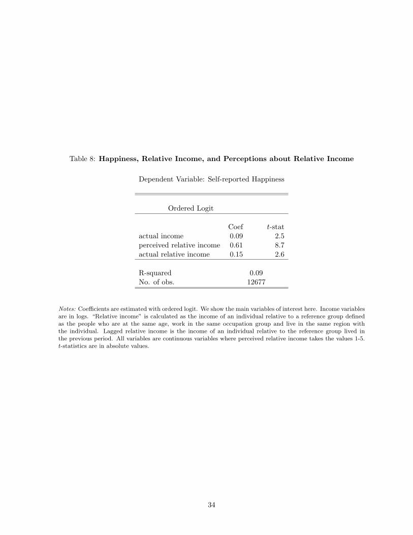
Table 8: Happiness, Relative Income, and Perceptions about Relative Income

Dependent Variable: Self-reported Happiness

Ordered Logit

Coef t-statactual income 0.09 2.5perceived relative income 0.61 8.7actual relative income 0.15 2.6

R-squared 0.09No. of obs. 12677

Notes: Coefficients are estimated with ordered logit. We show the main variables of interest here. Income variablesare in logs. “Relative income” is calculated as the income of an individual relative to a reference group definedas the people who are at the same age, work in the same occupation group and live in the same region withthe individual. Lagged relative income is the income of an individual relative to the reference group lived inthe previous period. All variables are continuous variables where perceived relative income takes the values 1-5.t-statistics are in absolute values.

34

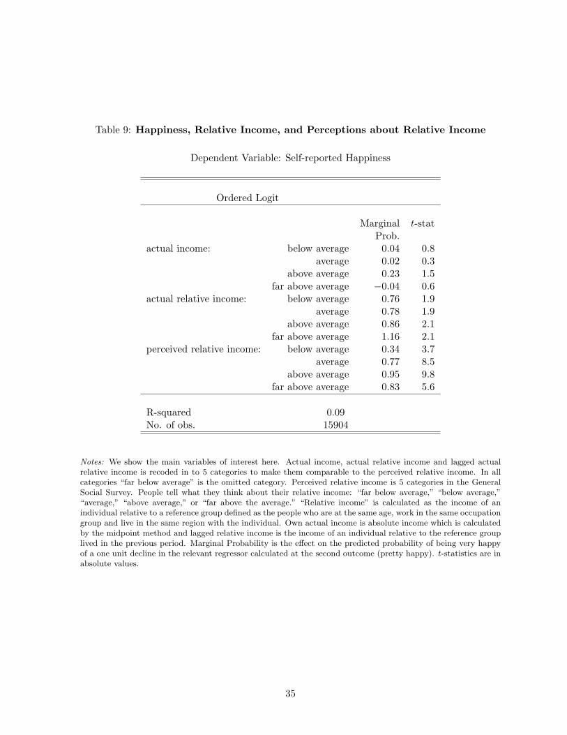
Table 9: Happiness, Relative Income, and Perceptions about Relative Income

Dependent Variable: Self-reported Happiness

Ordered Logit

Marginal t-statProb.

actual income: below average 0.04 0.8average 0.02 0.3

above average 0.23 1.5far above average −0.04 0.6

actual relative income: below average 0.76 1.9average 0.78 1.9

above average 0.86 2.1far above average 1.16 2.1

perceived relative income: below average 0.34 3.7average 0.77 8.5

above average 0.95 9.8far above average 0.83 5.6

R-squared 0.09No. of obs. 15904

Notes: We show the main variables of interest here. Actual income, actual relative income and lagged actualrelative income is recoded in to 5 categories to make them comparable to the perceived relative income. In allcategories “far below average” is the omitted category. Perceived relative income is 5 categories in the GeneralSocial Survey. People tell what they think about their relative income: “far below average,” “below average,”“average,” “above average,” or “far above the average.” “Relative income” is calculated as the income of anindividual relative to a reference group defined as the people who are at the same age, work in the same occupationgroup and live in the same region with the individual. Own actual income is absolute income which is calculatedby the midpoint method and lagged relative income is the income of an individual relative to the reference grouplived in the previous period. Marginal Probability is the effect on the predicted probability of being very happyof a one unit decline in the relevant regressor calculated at the second outcome (pretty happy). t-statistics are inabsolute values.

35

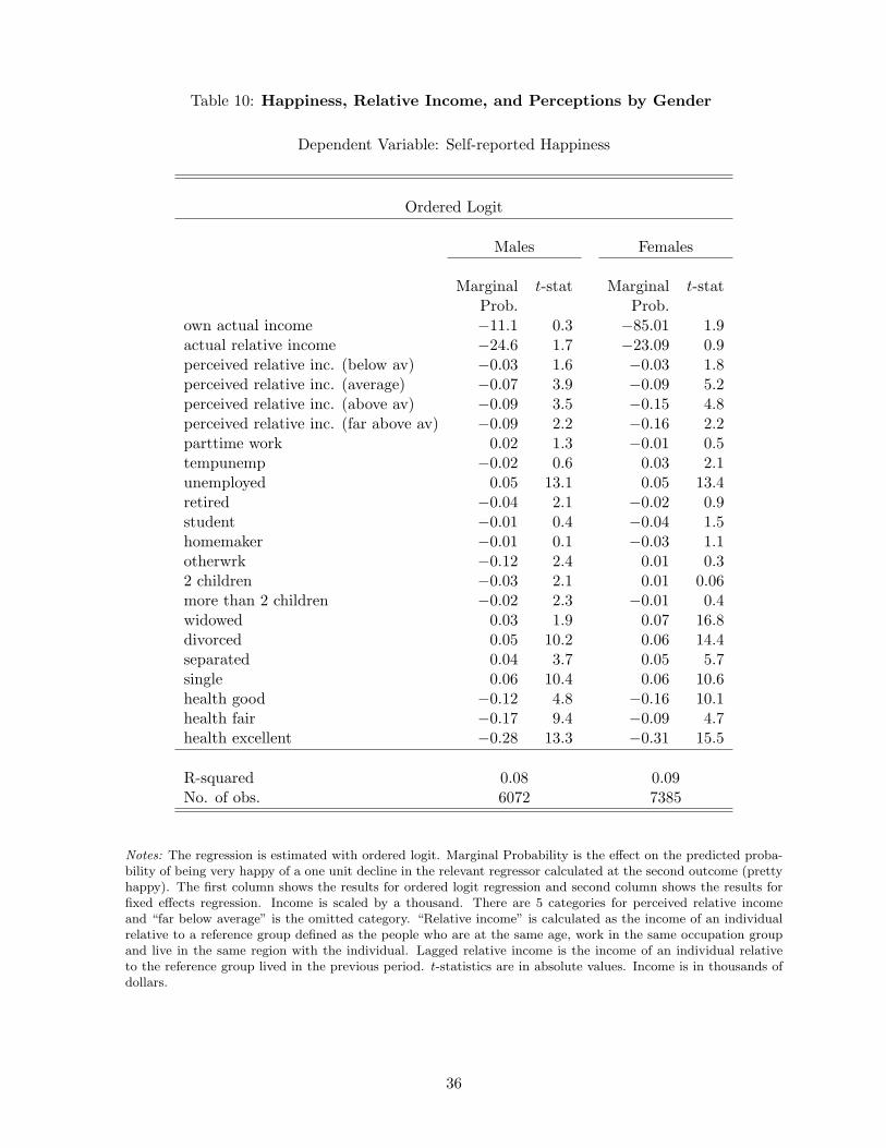
Table 10: Happiness, Relative Income, and Perceptions by Gender

Dependent Variable: Self-reported Happiness

Ordered Logit

Males Females

Marginal t-stat Marginal t-statProb. Prob.

own actual income −11.1 0.3 −85.01 1.9actual relative income −24.6 1.7 −23.09 0.9perceived relative inc. (below av) −0.03 1.6 −0.03 1.8perceived relative inc. (average) −0.07 3.9 −0.09 5.2perceived relative inc. (above av) −0.09 3.5 −0.15 4.8perceived relative inc. (far above av) −0.09 2.2 −0.16 2.2parttime work 0.02 1.3 −0.01 0.5tempunemp −0.02 0.6 0.03 2.1unemployed 0.05 13.1 0.05 13.4retired −0.04 2.1 −0.02 0.9student −0.01 0.4 −0.04 1.5homemaker −0.01 0.1 −0.03 1.1otherwrk −0.12 2.4 0.01 0.32 children −0.03 2.1 0.01 0.06more than 2 children −0.02 2.3 −0.01 0.4widowed 0.03 1.9 0.07 16.8divorced 0.05 10.2 0.06 14.4separated 0.04 3.7 0.05 5.7single 0.06 10.4 0.06 10.6health good −0.12 4.8 −0.16 10.1health fair −0.17 9.4 −0.09 4.7health excellent −0.28 13.3 −0.31 15.5

R-squared 0.08 0.09No. of obs. 6072 7385

Notes: The regression is estimated with ordered logit. Marginal Probability is the effect on the predicted proba-bility of being very happy of a one unit decline in the relevant regressor calculated at the second outcome (prettyhappy). The first column shows the results for ordered logit regression and second column shows the results forfixed effects regression. Income is scaled by a thousand. There are 5 categories for perceived relative incomeand “far below average” is the omitted category. “Relative income” is calculated as the income of an individualrelative to a reference group defined as the people who are at the same age, work in the same occupation groupand live in the same region with the individual. Lagged relative income is the income of an individual relativeto the reference group lived in the previous period. t-statistics are in absolute values. Income is in thousands ofdollars.

36

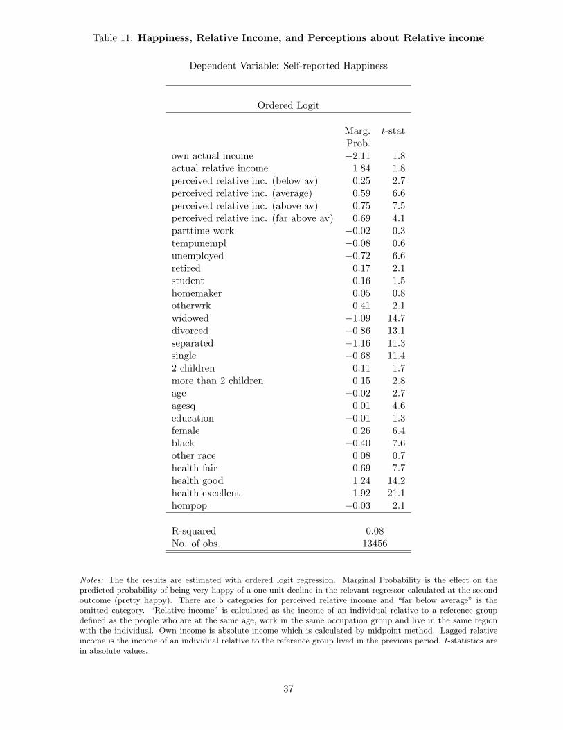
Table 11: Happiness, Relative Income, and Perceptions about Relative income

Dependent Variable: Self-reported Happiness

Ordered Logit

Marg. t-statProb.

own actual income −2.11 1.8actual relative income 1.84 1.8perceived relative inc. (below av) 0.25 2.7perceived relative inc. (average) 0.59 6.6perceived relative inc. (above av) 0.75 7.5perceived relative inc. (far above av) 0.69 4.1parttime work −0.02 0.3tempunempl −0.08 0.6unemployed −0.72 6.6retired 0.17 2.1student 0.16 1.5homemaker 0.05 0.8otherwrk 0.41 2.1widowed −1.09 14.7divorced −0.86 13.1separated −1.16 11.3single −0.68 11.42 children 0.11 1.7more than 2 children 0.15 2.8age −0.02 2.7agesq 0.01 4.6education −0.01 1.3female 0.26 6.4black −0.40 7.6other race 0.08 0.7health fair 0.69 7.7health good 1.24 14.2health excellent 1.92 21.1hompop −0.03 2.1

R-squared 0.08No. of obs. 13456

Notes: The the results are estimated with ordered logit regression. Marginal Probability is the effect on thepredicted probability of being very happy of a one unit decline in the relevant regressor calculated at the secondoutcome (pretty happy). There are 5 categories for perceived relative income and “far below average” is theomitted category. “Relative income” is calculated as the income of an individual relative to a reference groupdefined as the people who are at the same age, work in the same occupation group and live in the same regionwith the individual. Own income is absolute income which is calculated by midpoint method. Lagged relativeincome is the income of an individual relative to the reference group lived in the previous period. t-statistics arein absolute values.

37

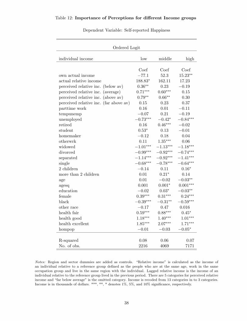
Table 12: Importance of Perceptions for different Income groups

Dependent Variable: Self-reported Happiness

Ordered Logit

individual income low middle high

Coef Coef Coefown actual income −77.1 52.3 15.23∗∗

actual relative income 188.83∗ 162.11 17.23perceived relative inc. (below av) 0.36∗∗ 0.23 −0.19perceived relative inc. (average) 0.71∗∗∗ 0.60∗∗∗ 0.15perceived relative inc. (above av) 0.79∗∗ 0.66∗∗ 0.30perceived relative inc. (far above av) 0.15 0.23 0.37parttime work 0.16 0.01 −0.11tempunemp −0.07 0.21 −0.19unemployed −0.73∗∗∗ −0.42∗ −0.84∗∗∗

retired 0.16 0.46∗∗∗ −0.02student 0.53∗ 0.13 −0.01homemaker −0.12 0.18 0.04otherwrk 0.11 1.35∗∗∗ 0.06widowed −1.01∗∗∗ −1.13∗∗∗ −1.18∗∗∗

divorced −0.99∗∗∗ −0.92∗∗∗ −0.74∗∗∗

separated −1.14∗∗∗ −0.92∗∗∗ −1.41∗∗∗

single −0.68∗∗∗ −0.78∗∗∗ −0.64∗∗∗

2 children −0.14 0.11 0.16∗

more than 2 children 0.01 0.21∗ 0.14age 0.01 −0.02 −0.03∗∗

agesq 0.001 0.001∗ 0.001∗∗∗

education −0.02 0.03∗ −0.03∗∗

female 0.39∗∗∗ 0.31∗∗∗ 0.24∗∗∗

black −0.39∗∗∗ −0.31∗∗ −0.59∗∗∗

other race −0.17 0.47 0.016health fair 0.59∗∗∗ 0.88∗∗∗ 0.45∗

health good 1.18∗∗∗ 1.40∗∗∗ 1.01∗∗∗

health excellent 1.85∗∗∗ 2.07∗∗∗ 1.71∗∗∗

hompop −0.01 −0.03 −0.05∗

R-squared 0.08 0.06 0.07No. of obs. 2216 4069 7171

Notes: Region and sector dummies are added as controls. “Relative income” is calculated as the income ofan individual relative to a reference group defined as the people who are at the same age, work in the sameoccupation group and live in the same region with the individual. Lagged relative income is the income of anindividual relative to the reference group lived in the previous period. There are 5 categories for perceived relativeincome and “far below average” is the omitted category. Income is recoded from 13 categories in to 3 categories.Income is in thousands of dollars. ***, **, * denotes 1%, 5%, and 10% significance, respectively.

38

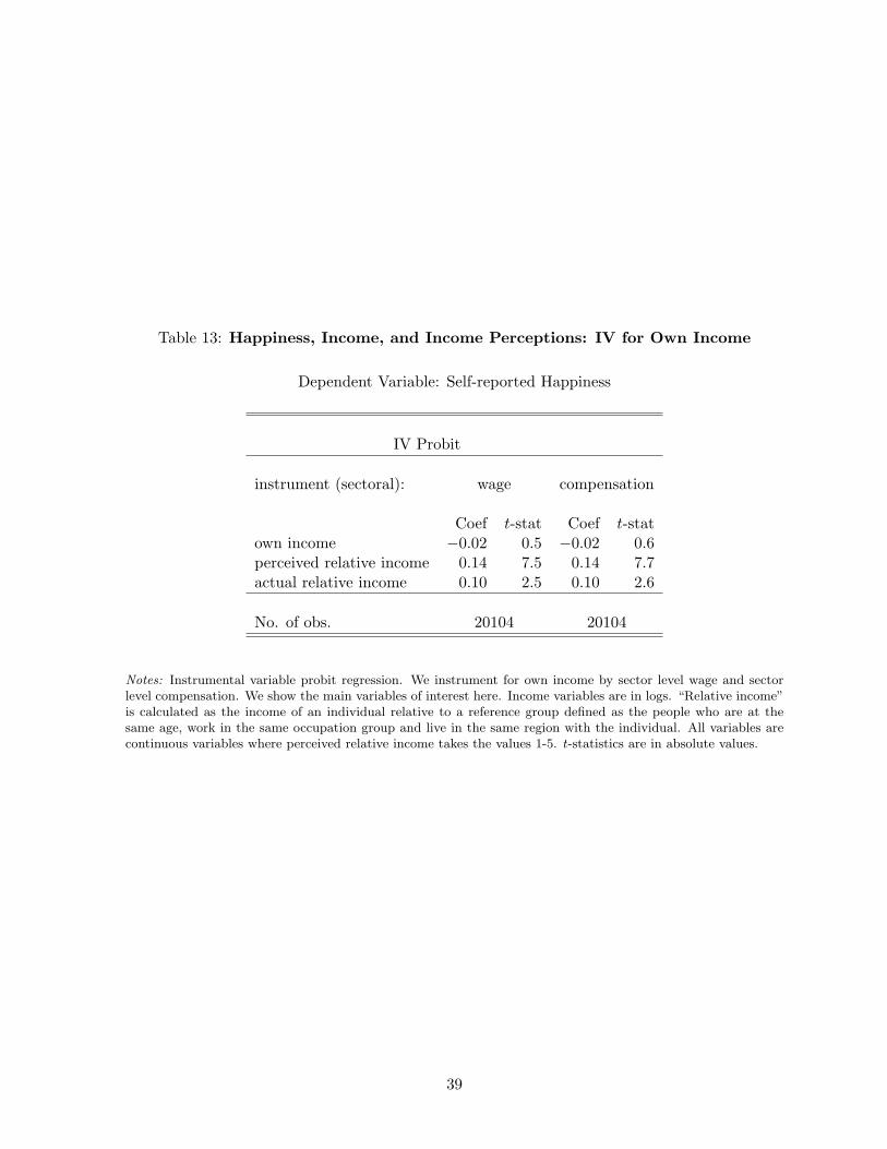
Table 13: Happiness, Income, and Income Perceptions: IV for Own Income

Dependent Variable: Self-reported Happiness

IV Probit

instrument (sectoral): wage compensation

Coef t-stat Coef t-statown income −0.02 0.5 −0.02 0.6perceived relative income 0.14 7.5 0.14 7.7actual relative income 0.10 2.5 0.10 2.6

No. of obs. 20104 20104

Notes: Instrumental variable probit regression. We instrument for own income by sector level wage and sectorlevel compensation. We show the main variables of interest here. Income variables are in logs. “Relative income”is calculated as the income of an individual relative to a reference group defined as the people who are at thesame age, work in the same occupation group and live in the same region with the individual. All variables arecontinuous variables where perceived relative income takes the values 1-5. t-statistics are in absolute values.

39

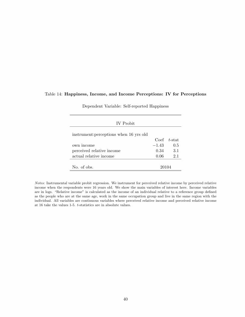
Table 14: Happiness, Income, and Income Perceptions: IV for Perceptions

Dependent Variable: Self-reported Happiness

IV Probit

instrument:perceptions when 16 yrs oldCoef t-stat

own income −1.43 0.5perceived relative income 0.34 3.1actual relative income 0.06 2.1

No. of obs. 20104

Notes: Instrumental variable probit regression. We instrument for perceived relative income by perceived relativeincome when the respondents were 16 years old. We show the main variables of interest here. Income variablesare in logs. “Relative income” is calculated as the income of an individual relative to a reference group definedas the people who are at the same age, work in the same occupation group and live in the same region with theindividual. All variables are continuous variables where perceived relative income and perceived relative incomeat 16 take the values 1-5. t-statistics are in absolute values.

40

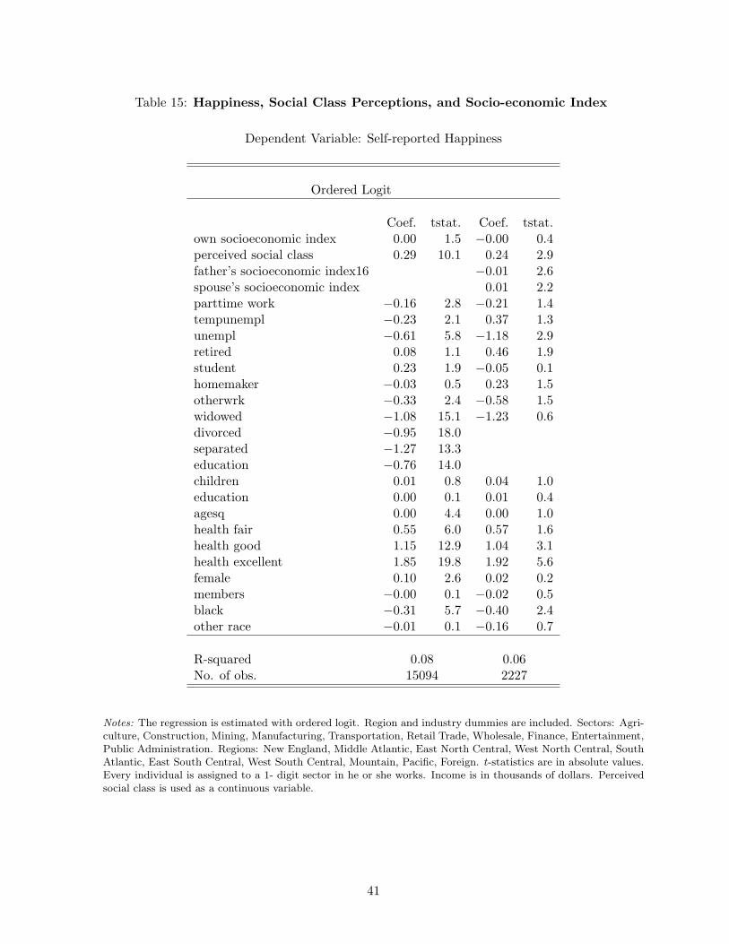
Table 15: Happiness, Social Class Perceptions, and Socio-economic Index

Dependent Variable: Self-reported Happiness

Ordered Logit

Coef. tstat. Coef. tstat.own socioeconomic index 0.00 1.5 −0.00 0.4perceived social class 0.29 10.1 0.24 2.9father’s socioeconomic index16 −0.01 2.6spouse’s socioeconomic index 0.01 2.2parttime work −0.16 2.8 −0.21 1.4tempunempl −0.23 2.1 0.37 1.3unempl −0.61 5.8 −1.18 2.9retired 0.08 1.1 0.46 1.9student 0.23 1.9 −0.05 0.1homemaker −0.03 0.5 0.23 1.5otherwrk −0.33 2.4 −0.58 1.5widowed −1.08 15.1 −1.23 0.6divorced −0.95 18.0separated −1.27 13.3education −0.76 14.0children 0.01 0.8 0.04 1.0education 0.00 0.1 0.01 0.4agesq 0.00 4.4 0.00 1.0health fair 0.55 6.0 0.57 1.6health good 1.15 12.9 1.04 3.1health excellent 1.85 19.8 1.92 5.6female 0.10 2.6 0.02 0.2members −0.00 0.1 −0.02 0.5black −0.31 5.7 −0.40 2.4other race −0.01 0.1 −0.16 0.7

R-squared 0.08 0.06No. of obs. 15094 2227

Notes: The regression is estimated with ordered logit. Region and industry dummies are included. Sectors: Agri-culture, Construction, Mining, Manufacturing, Transportation, Retail Trade, Wholesale, Finance, Entertainment,Public Administration. Regions: New England, Middle Atlantic, East North Central, West North Central, SouthAtlantic, East South Central, West South Central, Mountain, Pacific, Foreign. t-statistics are in absolute values.Every individual is assigned to a 1- digit sector in he or she works. Income is in thousands of dollars. Perceivedsocial class is used as a continuous variable.

41

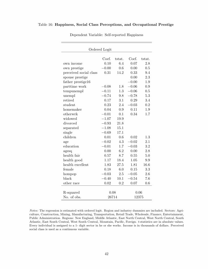
Table 16: Happiness, Social Class Perceptions, and Occupational Prestige

Dependent Variable: Self-reported Happiness

Ordered Logit

Coef. tstat. Coef. tstat.own income 0.10 6.4 0.07 2.8own prestige −0.00 0.6 0.00 0.5perceived social class 0.31 14.2 0.33 9.4spouse prestige 0.00 2.3father prestige16 −0.00 1.9parttime work −0.08 1.8 −0.06 0.9tempunempl −0.11 1.3 −0.06 0.5unempl −0.74 9.8 −0.78 5.3retired 0.17 3.1 0.29 3.4student 0.23 2.4 −0.03 0.2homemaker 0.04 0.9 0.11 1.9otherwrk −0.01 0.1 0.34 1.7widowed −1.07 19.9divorced −0.93 21.8separated −1.08 15.1single −0.69 17.1children 0.01 0.6 0.02 1.3age −0.02 4.3 −0.02 2.1education −0.01 1.7 −0.03 3.2agesq 0.00 6.2 0.00 2.8health fair 0.57 8.7 0.55 5.0health good 1.17 18.4 1.05 9.9health excellent 1.83 27.5 1.81 16.6female 0.18 6.0 0.15 3.3hompop −0.03 2.5 −0.05 2.6black −0.40 10.1 −0.54 7.6other race 0.02 0.2 0.07 0.6

R-squared 0.08 0.06No. of obs. 26714 12375

Notes: The regression is estimated with ordered logit. Region and industry dummies are included. Sectors: Agri-culture, Construction, Mining, Manufacturing, Transportation, Retail Trade, Wholesale, Finance, Entertainment,Public Administration. Regions: New England, Middle Atlantic, East North Central, West North Central, SouthAtlantic, East South Central, West South Central, Mountain, Pacific, Foreign. t-statistics are in absolute values.Every individual is assigned to a 1- digit sector in he or she works. Income is in thousands of dollars. Perceivedsocial class is used as a continuous variable.

42

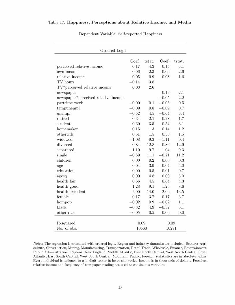
Table 17: Happiness, Perceptions about Relative Income, and Media

Dependent Variable: Self-reported Happiness

Ordered Logit

Coef. tstat. Coef. tstat.perceived relative income 0.17 4.2 0.15 3.1own income 0.06 2.3 0.06 2.6relative income 0.05 0.9 0.08 1.6TV hours −0.14 3.8TV*perceived relative income 0.03 2.6newspaper 0.13 2.1newspaper*perceived relative income −0.05 2.2parttime work −0.00 0.1 −0.03 0.5tempunempl −0.09 0.8 −0.09 0.7unempl −0.52 4.5 −0.64 5.4retired 0.34 2.1 0.28 1.7student 0.60 3.5 0.54 3.1homemaker 0.15 1.3 0.14 1.2otherwrk 0.51 1.5 0.53 1.5widowed −1.08 9.3 −1.11 9.4divorced −0.84 12.8 −0.86 12.9separated −1.10 9.7 −1.04 9.3single −0.69 11.1 −0.71 11.2children 0.00 0.2 0.00 0.3age −0.04 3.9 −0.04 4.0education 0.00 0.5 0.01 0.7agesq 0.00 4.8 0.00 5.0health fair 0.66 4.5 0.64 4.3health good 1.28 9.1 1.25 8.6health excellent 2.00 14.0 2.00 13.5female 0.17 3.7 0.17 3.7hompop −0.02 0.9 −0.02 1.1black −0.32 4.9 −0.37 6.1other race −0.05 0.5 0.00 0.0

R-squared 0.09 0.09No. of obs. 10560 10281

Notes: The regression is estimated with ordered logit. Region and industry dummies are included. Sectors: Agri-culture, Construction, Mining, Manufacturing, Transportation, Retail Trade, Wholesale, Finance, Entertainment,Public Administration. Regions: New England, Middle Atlantic, East North Central, West North Central, SouthAtlantic, East South Central, West South Central, Mountain, Pacific, Foreign. t-statistics are in absolute values.Every individual is assigned to a 1- digit sector in he or she works. Income is in thousands of dollars. Perceivedrelative income and frequency of newspaper reading are used as continuous variables.

43

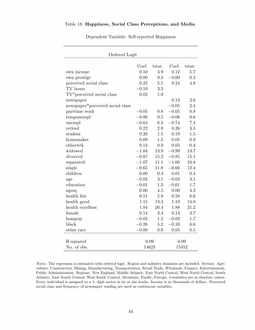
Table 18: Happiness, Social Class Perceptions, and Media

Dependent Variable: Self-reported Happiness

Ordered Logit

Coef. tstat. Coef. tstat.own income 0.10 4.9 0.12 5.7own prestige 0.00 0.3 −0.00 0.2perceived social class 0.25 5.5 0.24 4.8TV hours −0.10 3.3TV*perceived social class 0.02 1.9newspaper 0.13 2.6newspaper*perceived social class −0.05 2.4parttime work −0.05 0.8 −0.05 0.8tempunempl −0.06 0.5 −0.06 0.6unempl −0.64 6.3 −0.74 7.4retired 0.22 2.9 0.26 3.5student 0.20 1.5 0.19 1.5homemaker 0.09 1.5 0.05 0.9otherwrk 0.14 0.9 0.05 0.4widowed −1.04 13.9 −0.99 13.7divorced −0.87 15.2 −0.85 15.1separated −1.07 11.1 −1.00 10.8single −0.65 11.8 −0.66 12.4children 0.00 0.3 0.01 0.4age −0.02 3.1 −0.02 3.1education −0.01 1.3 −0.01 1.7agesq 0.00 4.5 0.00 4.3health fair 0.51 5.8 0.58 6.6health good 1.15 13.3 1.19 14.0health excellent 1.84 20.4 1.88 21.2female 0.14 3.4 0.14 3.7hompop −0.02 1.2 −0.02 1.7black −0.28 5.2 −0.33 6.6other race −0.00 0.0 0.05 0.5

R-squared 0.09 0.09No. of obs. 14623 15452

Notes: The regression is estimated with ordered logit. Region and industry dummies are included. Sectors: Agri-culture, Construction, Mining, Manufacturing, Transportation, Retail Trade, Wholesale, Finance, Entertainment,Public Administration. Regions: New England, Middle Atlantic, East North Central, West North Central, SouthAtlantic, East South Central, West South Central, Mountain, Pacific, Foreign. t-statistics are in absolute values.Every individual is assigned to a 1- digit sector in he or she works. Income is in thousands of dollars. Perceivedsocial class and frequency of newspaper reading are used as continuous variables.

44