Embed Size (px)
Citation preview

Statistics with R
http://web.abo.fi/fak/mnf/mate/kurser/statisticsr/
Prepared by José Gama, MSc
Department of MathematicsÅbo Akademi University

References:
"A Practical Guide to Geostatistical Mapping of Environmental Variables", Tomislav Hengl, Joint Research Centr, Institute for Environment and Sustainability pp. 56, 80
The R Core Team, "What is R?", R News, Volume 1/1, January 2001
http://cran.r-project.org/doc/html/interface98-paper/paper_2.html
http://en.wikipedia.org/wiki/R_%28programming_language%29

Believe nothing merely because you have been told it.Do not believe what your teacher tells you merely out of respect for the teacher.But whatever, after due examination and analysis, you find to be kind, conducive to the good, the benefit, the welfare of all beings - that doctrine believe and cling to, and take it as your guide.
However many holy words you read, however many you speak, what good will they do you if you do not act on upon them?
There are only two mistakes one can make along the road to truth; not going all the way, and not starting.
What we think, we become.
Buddha, spiritual teacher from India

I hear and I forget. I see and I remember. I do and I understand.
Confucius
Chinese philosopher & reformer (551 BC - 479 BC)

Revision of R/statistical concepts
Examples of reviewed R/statistical concepts
R commands to work on these concepts
Questions, to be solved with R, by the students
Answers and explanations before moving on
How the classes will be organized
Course structure
The course will be 14 lessons of 2 hours each.
The class starts 10 minutes after the scheduled hour.
The grade is pass/fail.
To pass, a student must attend 11 lessons and answer correctly 10 questions from the questionnaire.
Alternatively, a student must answer correctly 15 questions from the questionnaire.
The reading assignments are optional but recommended, in particular for students who will not attend the class.
The online material is enough to learn the basics and answer the questionnaire.
The classes will cover more details and have from 5 to 10 times more examples than the online material. This can be exhausting, but you must ask if you want something explained differently or if you need a break.
The classes will also be more friendly to students not from Computer Science, unlike the online material.

Course structure
R has many strong points, two of which are its great help system and available packages.
However, many students complaint that, after an introductory course on R, they are not comfortable with using the help or packages.
Usually it doesn't matter because they will never use R again or use it only for a few histograms or boxplots, once in a blue moon.
Students from Statistics, Bioinformatics and Environmental Sciences will have to work with many packages and find help on any topic without assistance.
That is why the initial lessons will be long and boring, but necessary to get solid foundations on R.

The R Project for Statistical Computing
“R is a free software environment for statistical computing and graphics. It compiles and runs on a wide variety of UNIX platforms, Windows and MacOS.”
“R is an integrated suite of software facilities for data manipulation, calculation and graphical display. It includes an effective data handling and storage facility,a suite of operators for calculations on arrays, in particular matrices, a large, coherent, integrated collection of intermediate tools for data analysis, graphical facilities for data analysis and display either on-screen or on hardcopy, and a well-developed, simple and effective programming language which includes conditionals, loops, user-defined recursive functions and input and output facilities. ”
http://www.r-project.org/

What is R
R is a software environment and programming language for statistical computing and graphics. R is the open source equivalent to the programming language S.S is very popular on statistical methodology research and was developed by John Chambers and, previously, by Rick Becker and Allan Wilks of Bell Laboratories.The name "R" comes from the fact that "R" precedes "S" and both authors' names start with "R", Ross Ihaka and Robert Gentleman. The R basic distribution comes with plenty of statistical procedures such as: linear and generalized linear models, nonlinear regression models, time series analysis, classical parametric and nonparametric tests, clustering and smoothing. There are many graphical procedures such as: plot, scatterplot, boxplot, distribution-comparison plot, histogram, dotchart, contour lines, 3D surface, etc...R is extensible with a multitude of packages, some of them for very specialized areas or highly optimized for intensive computations. R is a programming language, allowing object-oriented programming (OOP) and with lexical (static) scoping semantics similar to Scheme (dialect of Lisp). C, C++, and Fortran code can be linked and called at run time, adding more power and flexibility.
The history of R
R was developed by Ross Ihaka and Robert Gentleman at the University of Auckland, New Zealand.Ross Ihaka read the book "The Structure and Interpretation of Computer Programs" about the Scheme programming language. Later, he tried to use lexical scope, to obtain own variables, in S, which didn't work because of the differences in the scoping rules of S and Scheme. Years passed, and Robert Gentleman and Ross Ihaka were at the University of Auckland, both working on statistical computing. They decided to create a small Scheme-like interpreter, to be used as a software environment. It was similar to S in syntax because Scheme and S are similar and both authors were familiar with S.There was a first release in August of 1993. In June of 1995, the source code was distributed under the terms of the Free Software Foundation's GNU general license (GPL).The interest kept growing and a small mailing list to exchange ideas had to grow to a larger automated mailing list, then to newsgroups and the distribution of code, documentation and binaries expanded to more mirror sites. Finally, the core group of developers had to grow, as well.In 2001, Robert Gentleman started the project Bioconductor that uses statistical computing, with R, in Computational Biology.

Portable R
R is "perfectly relocatable", that is, after being installed in one machine, the directory can be copied, for example, to a memory stick and it will run from there. Notes:Installing packages - download the package from CRAN, use Packages -> Install Package(s) from local zip file(s)workspace and history can be relocated by copying .Rhistory and .RData
http://my.opera.com/semin/blog/2007/04/02/portable-r
Portable GIS
Runs from a memory stick. Contents:●Desktop GIS packages GRASS (windows native version 6.3: does not need cygwin), QGIS (version 0.10 with GRASS plugin) and gvSIG (version 1.1),●FWTools (GDAL and OGR toolkit, version 2.10)●XAMPPlite (Apache2/MySQL5/Php5),●PostgreSQL (version 8.2)/Postgis (version 1.1),●Mapserver, OpenLayers, Tilecache, Featureserver, and Geoserver web applications.
http://www.archaeogeek.com/blog/portable-gis/

Portable GIMP
The GIMP (GNU Image Manipulation Program), Open Source image editor in a portable version:
http://portableapps.com/apps/graphics_pictures/gimp_portable
OpenOffice.org Portable
OpenOffice.org Portable is a complete OpenOffice.org office suite, compatible with Microsoft Office, Word Perfect, Lotus and other office applications.Includes:●Word processor●Spreadsheet●Presentation tool●Drawing package●Database
http://portableapps.com/apps/office/openoffice_portable

Two students sharing one computer
Open two R windows and change the working directory on both:

Two students sharing one computer
If the default is user\Documents Click Make New Folder and name it user1
Do the same for the other R window but creating a directory user2

Two students sharing one computer
Change the working directory on the other R window:

Two students sharing one computer
If the default is user\Documents Click Make New Folder and name it user2
Two students sharing one computer
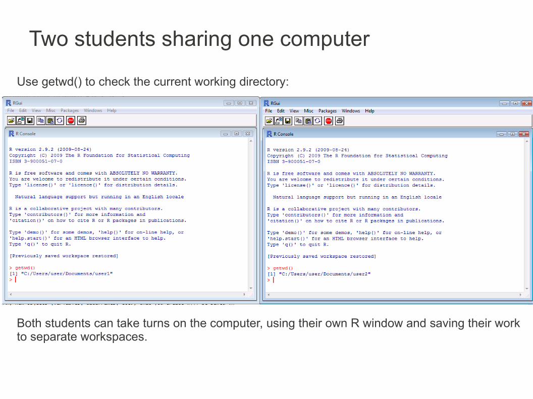
Use getwd() to check the current working directory:
Both students can take turns on the computer, using their own R window and saving their work to separate workspaces.

Downloading and Installing R
The R Project for Statistical Computing Homepage:http://www.r-project.org/
That page has a link to anther page with the CRAN mirrors

Scrolling down the list, there are links to Sweden, UK and the US, among many others
Scroll down to Sweden
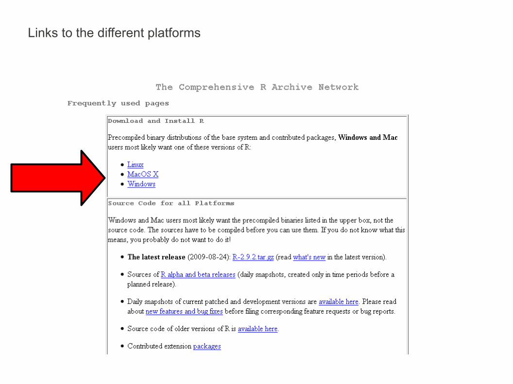
Links to the different platforms

Let's download the Windows version (base)

Installing the Windows version (base)
Download R-2.9.2-win32.exe (the 2.9.2 is the version number, it might be different) and execute it. There are several languages that can be used during the installation, which is very straightforward.

Installing the Windows version (base)

On Fedora 10, as root:yum install R
On Fedora 8 or 9, as root:yum install R R-devel
Installing the Linux version
More info here

On Ubuntu:
gpg --keyserver subkeys.pgp.net --recv-key E2A11821gpg -a --export E2A11821 | sudo apt-key add -
sudo gedit /etc/apt/sources.listAdd this line to the bottom of the sources.list file:deb http://rh-mirror.linux.iastate.edu/CRAN/bin/linux/ubuntu hardy/Use your own: feisty or jaunty, etc... instead of hardySave the file and go back to the Bash terminal.
sudo apt-get update
sudo apt-get install r-base r-base-dev
From: https://stat.ethz.ch/pipermail/r-help/2009-February/187644.html
Installing the Linux version

Installing the MacOSX version
First, download "R-2.9.2.dmg" from the "bin/macosx" directory of a CRAN site
Double-click on the icon to mount the disk image file
http://blogs.oreilly.com/digitalmedia/2008/06/free-statistics-package-for-yo.html

Installing R
References/to learn more:
The R bookMichael J. Crawley pp 12007 John Wiley & Sons Ltd
Basic statistics using R pp. 8Jarno Tuimala (CSC) and Dario Greco (HY)http://www.csc.fi/english/csc/courses/archive/R2008s
Statistics with RVincent Zoonekynd, pp 3http://zoonek2.free.fr/UNIX/48_R/all.html
Aprendizaje del software estadístico R: un entorno para simulación y computación estadísticaProf. Alberto muñoz garcíaDepartamento de EstadísticaUniversidad Carlos III de Madridhttp://ocw.uc3m.es/estadistica/aprendizaje-del-software-estadistico-r-un-entorno-para-simulacion-y-computacion-estadistica/introduccion-al-analisis-de-datos-y-al-lenguaje-s
Geographic Data AnalysisPat Bartleinhttp://geography.uoregon.edu/bartlein/courses/geog417/exercises/ex1.htm
Software Tools, Part 1: introduction to R softwarePetri Koistinenhttp://www.rni.helsinki.fi/~pek/s-tools/RGetToKnow.html
Chem 351 Archives PageDavid Harveyhttp://fs6.depauw.edu:50080/~harvey/Chem%20351/PDF%20Files/Handouts/RDocs/Obtaining%20and%20Installing%20R.pdf

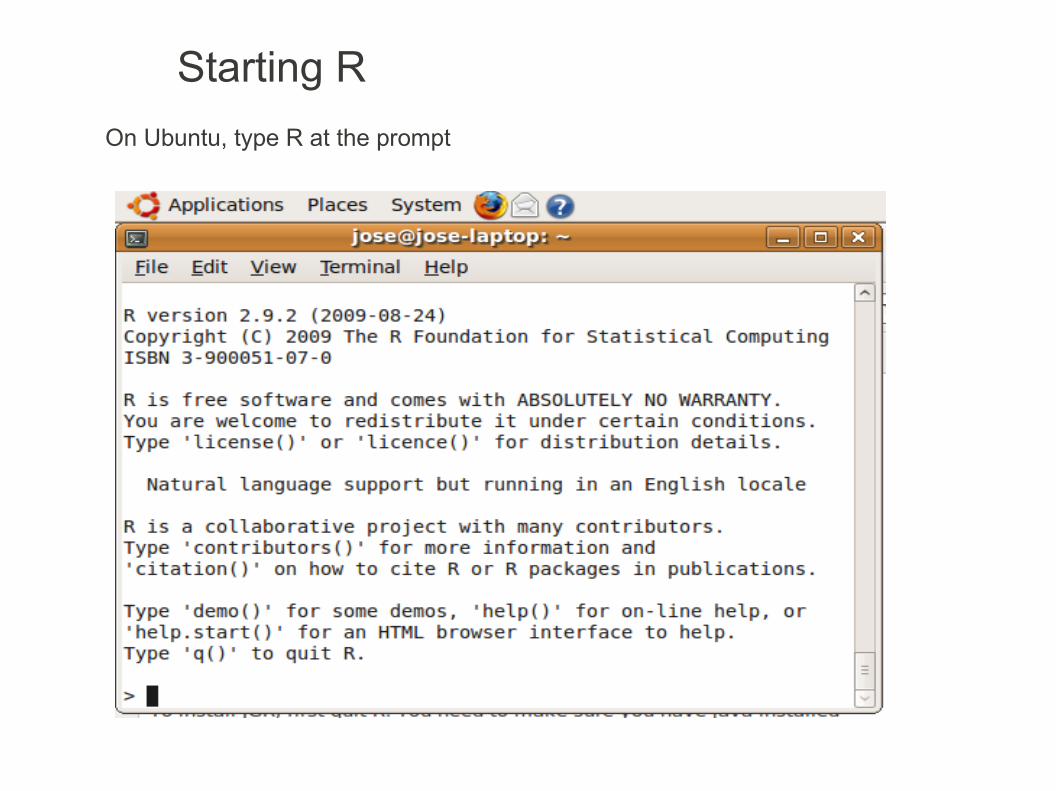
Starting R
On Windows, if there is a shortcut on the desktop:
Or on the Start menu:
Starting R
On Ubuntu, type R at the prompt

Starting R
On Fedora, type R at the prompt

Rgui
Load R functions
Open the R editor
Open a file on the R editor
Display text file(s)
Print the History
Save the History as text
History is the text on the console:
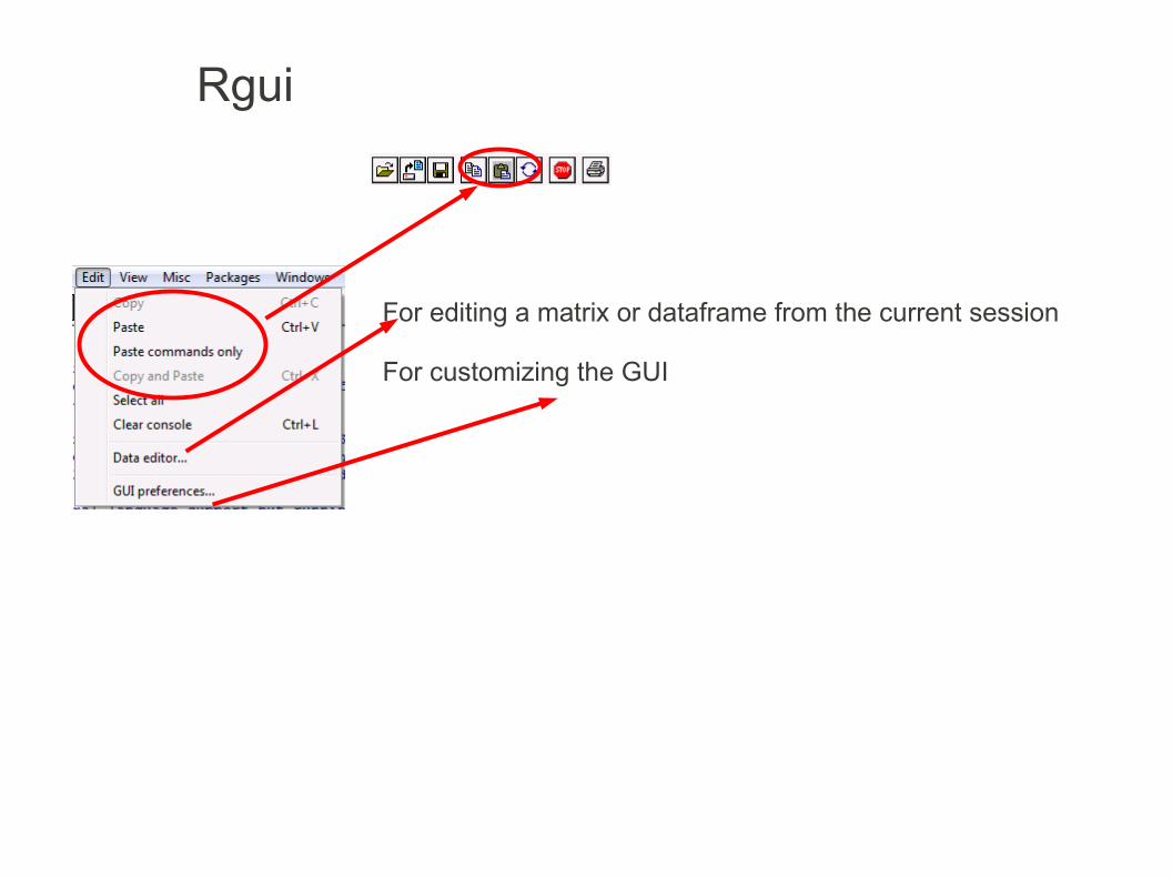
For editing a matrix or dataframe from the current session
For customizing the GUI
Rgui

Data Editor
For editing a matrix or dataframe from the current session
Same as the fix function
The cells are editable, like a spreadsheet
Rgui

RguiCustomizing the GUI
Some editors will only work with MDI
Buffer chars and Lines can be increased if it is necessary to work with a long History and there is an error because there is no space for it
This will apply the changes to the current session
To make changes permanent, that is, for every session,they must be saved. The default file Rconsole is loaded when a session starts
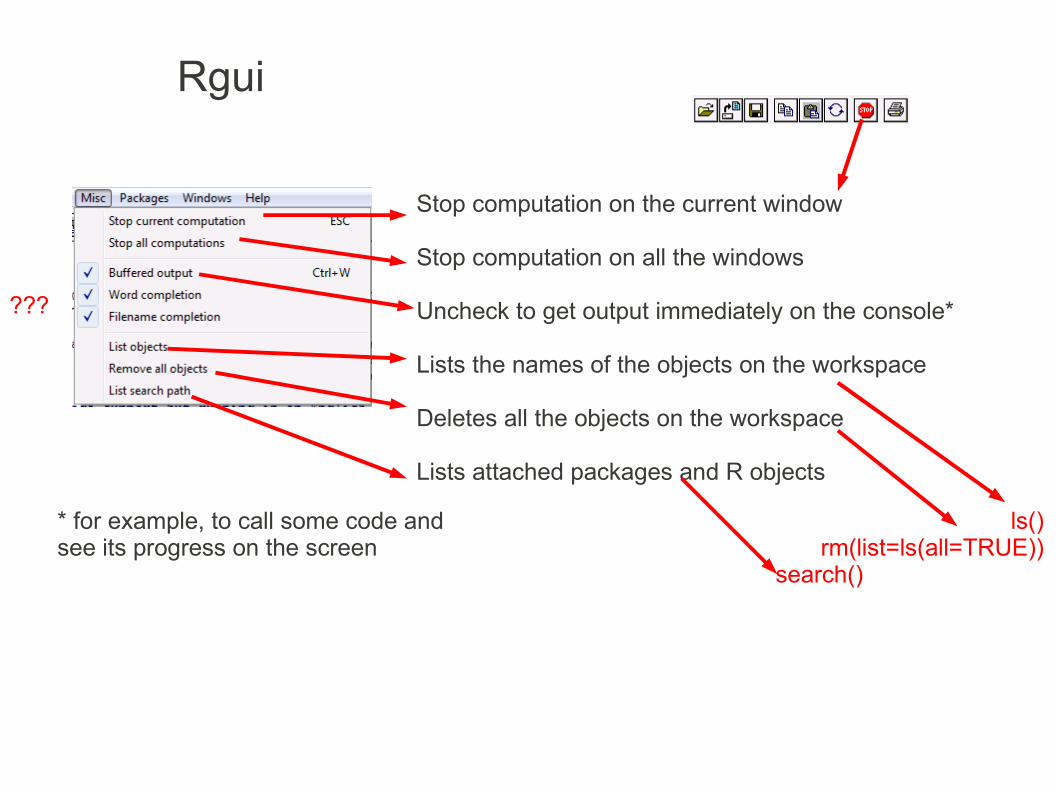
Rgui
Stop computation on the current window
Stop computation on all the windows
Uncheck to get output immediately on the console*
Lists the names of the objects on the workspace
Deletes all the objects on the workspace
Lists attached packages and R objects
* for example, to call some code and see its progress on the screen
ls()rm(list=ls(all=TRUE))
search()
???

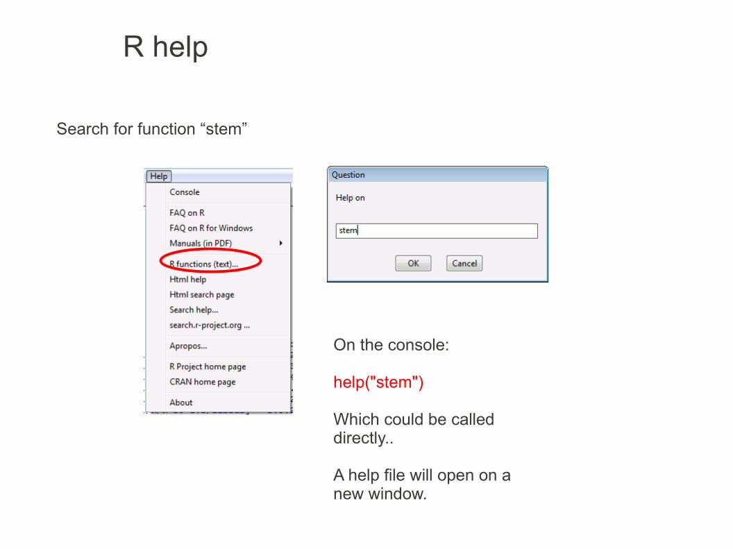
R help
Help about the console controls
Help about a known function name
R HTML manuals and references
R HTML search engine for keywords, function and data names and text in help page titles
Search a reference from the manual
Use the online R Site Search
Look for a function name, partially known
help("plot")?plot
help.start()
help.search("test")??test
RSiteSearch("test")
apropos(“test”)
From the console:
R help
On the console:
help("stem")
Which could be called directly..
A help file will open on a new window.
Search for function “stem”

R helpFunction stem was found
Description of what the function does
Function call with arguments
Description of arguments, sometimes with links to related objects
References to literature
How to use the function, the two examples provided will run automatically:
example("stem")

R help
It doesn't show on the console but the equivalent command is:
help.start()
A new tab will open on the browser with the HTML help page.
R HTML manuals and references

R help
Manuals in HTML format
Very complete introduction to R
Installing and customizing R

R help
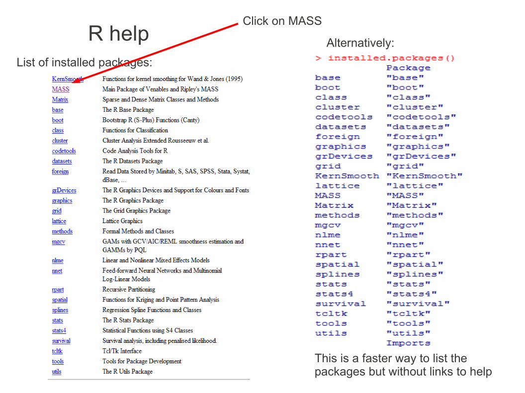
List of installed packages:
R helpList of installed packages:
Alternatively:
Click on MASS
This is a faster way to list the packages but without links to help
R help
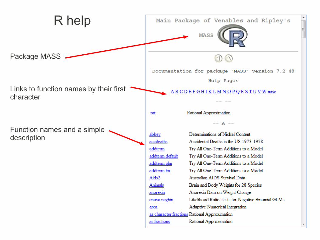
Package MASS
Links to function names by their first character
Function names and a simple description

R help
It doesn't show on the console but the equivalent command would be:
help.start()
Followed by clicking the link
Search Engine & Keywords
R HTML search engine

R help
Search for a reference from the manual on the keyword “test”
From the prompt:
help.search("test")
or
??test

R help
From the prompt:
RsiteSearch("test")
Use the online R Site Search

R help
From the prompt:
apropos(“test”)
Look for a function name, partially known
Try this:apropos("test")apropos(".test")apropos("[\\.]test")apropos("[^\\.]test")apropos("^test")apropos("([^\\.]test)|(^test)")

R helpapropos("test")apropos(".test")apropos("[\\.]test")apropos("[^\\.]test")apropos("^test")apropos("([^\\.]test)|(^test)")
1. “test” is anywhere within the function name
2. find “test” preceded by any character
3. find “.test”
4. find “test” preceded by any character, other than “.”
5. find “test”, only if at the end of the name
6. both 4. and 5.Remember:Apropos uses regular expressions for searches

R helpHow to use help
To show the documentationhelp() or ?help
To find the documentation about the function "plot"?plothelp("plot")
To find the documentation about reserved words or non-alphanumeric commands?"for"?"[["?"[<-.data.frame"
To find all the installed help files (packages) that have an alias, concept or title named "plot"??plothelp.search("plot")
Package "graphics" has a function "plot", let's examine it:?graphics::plotPackage "lattice" has a function "xyplot", let's examine it:?lattice::xyplot
To get a short description of a package:library(help = graphics)
Use double quotes

R help
How to use help
When not sure about the function name (on the search path), but it contains "plot"apropos("plot")
To search R the web site and the R-help mailing list (http://search.r-project.org)RSiteSearch("plot")
To run the examples from a help topicexample(topic)
To find where there are some demos for the loaded packagesdemo()
To find where there are some demos for all the packagesdemo(package = .packages(all.available = TRUE))
To show the demo "graphics" from package "graphics", pausing between pagesdemo(graphics, package="graphics", ask=TRUE)
To show the demo "graphics" from package "graphics", whithout pausing between pagesdemo(graphics, package="graphics", ask=FALSE)

Other sources of help
R Project search enginehttp://www.r-seek.org
mailing lists which are used by R users and developers. Seehttp://www.R-project.org/mail.html
Bug-tracking systemR has a bug-tracking system (or perhaps a bug-filing system is a more precise description) available on the net athttp://bugs.R-project.org/
The R Journalhttp://journal.r-project.org/
Journal of Statistics Educationhttp://www.amstat.org/PUBLICATIONS/JSE/
Technology Innovations in Statistics Educationhttp://repositories.cdlib.org/uclastat/cts/tise/
Journal of Statistical Softwarehttp://www.jstatsoft.org
R help

R help
Exercise
How to get random numbers in R?
Use only the help tools discussed today

R help
?random # no results...
??random
base::RNG Random Number Generationbase::sample Random Samples and Permutationsdatasets::randu Random Numbers from Congruential Generator RANDU
?base::RNG # Random Number Generation?base::sample # Random Samples and Permutations?datasets::randu # Random Numbers from Congruential Generator RANDU ("widely considered to be one of the most ill-conceived random number generators designed", Wikipedia)

The command-line editor
Recall and correction of previous commands
R keeps a command history, a list of the commands executed at the prompt.
Enter will execute the current line of text, at the prompt.
Cursor keys:Arrow up - show previous commandArrow down - show next commandArrows left and right - move around the current line of text, at the prompt.
Editor comands:

The command-line editor
R startup message
User expression
Result
Prompt, this is the input area

The command-line editorIncomplete expressions will result on an annoying + that will disappear once the expression is completed.
A string must be within enclosing double quotes but, pressing enter, will cause a newline character to be part of the string.
An expression is incomplete if it ends with an operator. There are no side effects, once the expression is completed.
An expression with parenthesis will not work, until all the parenthesis are paired. There are no side effects, once the expression is completed.

The command-line editor
The console will accept multiple commands, if pasted, and execute one line at a time.
For example, copying from Notepad:
And pasting on R:
This is unnecessary because R has its own text editor, the R Editor

The R Editor
Open the R editor
Open a file on the R editor
Run all the codeOpen R file
Save R fileRun current line
or selected code
Menu changes:
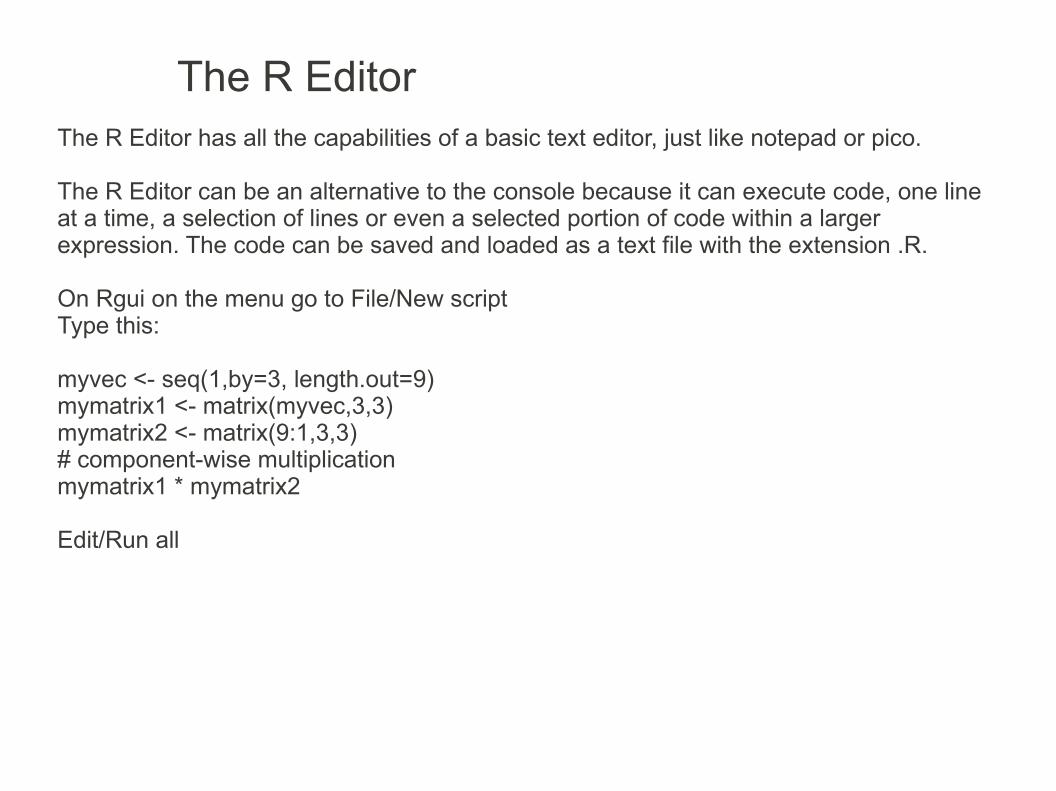
The R EditorThe R Editor has all the capabilities of a basic text editor, just like notepad or pico.
The R Editor can be an alternative to the console because it can execute code, one line at a time, a selection of lines or even a selected portion of code within a larger expression. The code can be saved and loaded as a text file with the extension .R.
On Rgui on the menu go to File/New scriptType this:
myvec <- seq(1,by=3, length.out=9)mymatrix1 <- matrix(myvec,3,3)mymatrix2 <- matrix(9:1,3,3)# component-wise multiplicationmymatrix1 * mymatrix2
Edit/Run all

The R Editor
Position the cursor on any line and press ctrl-r, the line of code will execute on the R console and the cursor will mode down to the next line. It is possible to follow the execution of code by pressing ctrl-r continuously.
myvec <- seq(1,by=3, length.out=9)|mymatrix1 <- matrix(myvec,3,3)mymatrix2 <- matrix(9:1,3,3)# component-wise multiplicationmymatrix1 * mymatrix2
Position the cursor at the beginning of any line and use shift+cursor keys or keep the left-click button on the mouse pressed and move the cursor, to select a few lines of code and press ctrl-r, the line of code will execute on the R console.
mymatrix2 <- matrix(9:1,3,3)# component-wise multiplicationmymatrix1 * mymatrix2
The cursor is on this line, ctrl-r will execute it
myvec <- seq(1,by=3, length.out=9)mymatrix1 <- matrix(myvec,3,3)

The R EditorPosition the cursor at the beginning of an expression and use shift+cursor keys or keep the left-click button on the mouse pressed and move the cursor, to select a valid expression and press ctrl-r, the expression will execute on the R console.
myvec <- seq(1,by=3, length.out=9)mymatrix1 <- matrix(myvec,3,3)mymatrix2 <- matrix(9:1,3,3)# component-wise multiplicationmymatrix1 * mymatrix2
myvec <- seq(1,by=3, length.out=9)mymatrix1 <- matrix(myvec,3,3)mymatrix2 <- matrix(9:1,3,3)# component-wise multiplicationmymatrix1 * mymatrix2
myvec <- seq(1,by=3, length.out=9)mymatrix1 <- matrix(myvec,3,3)mymatrix2 <- matrix(9:1,3,3)# component-wise multiplicationmymatrix1 * mymatrix2

Tinn-R, an editor with more options
http://jekyll.math.byuh.edu/other/howto/tinnr/using.shtml
Features:
●R console window access from within Tinn-R.●Incremental execution of R code.●Integrated R help.●R Object explorer.●Line number for a source file.●Search and Replace.●Current line highlighting. Etc...

Getting information about R and the system
To get the Rversion
To get the licenseinfo
To learn how to citeR in publications
info about theplatform underwhich R wasbuilt
system and userinformation
R.version license() citation() .Platform Sys.info()

Getting information about R and the system
To get a list of the installed packages
To get a list new packages available
version information about R and attached or loaded packages
numerical characteristics of the machine
names of open graphics devices
installed.packages()
old.packages()
sessionInfo() .Machine .Device

command line+R Editor
References/to learn more:
The R bookMichael J. Crawley pp 92008 John Wiley & Sons Ltd
Basic statistics using R pp. 34Jarno Tuimala (CSC) and Dario Greco (HY)http://www.csc.fi/english/csc/courses/archive/R2008s
Software Tools, Part 1: introduction to R softwarePetri Koistinenhttp://www.rni.helsinki.fi/~pek/s-tools/calculator.r
Chem 351 Archives PageDavid Harveyhttp://fs6.depauw.edu:50080/~harvey/Chem%20351/PDF%20Files/Handouts/RDocs/Some%20Basic%20R%20Commands.pdf
Packages
The base distribution of R is the R programming language interpreter and some packages that are loaded by default. Packages, AKA extensions, are libraries that can be installed and used when needed and extend the functionality of R by adding new objects, for example new statistical functions, and their documentation and even data.
A package is a zip file, containing a file with the description of the package and subdirectories with the source code of the package and other information such as documentation, configuration, license, etc... This is described on the manual "Writing R Extensions".Several projects distribute contributed packages, such as CRAN (The Comprehensive R Archive Network), Bioconductor (Analysis and comprehension of genomic data), OmegaHat (software for S, R and Xlisp-Stat), etc...
There are about 30 default packages, the base package has functions for the R programming language, other packages have functions for data input/output, graphics, utilities and statistical tools.
Packages are one of the strengths of R, with over 2000 packages available, therefore, there are many functions to handle packages.
Packages
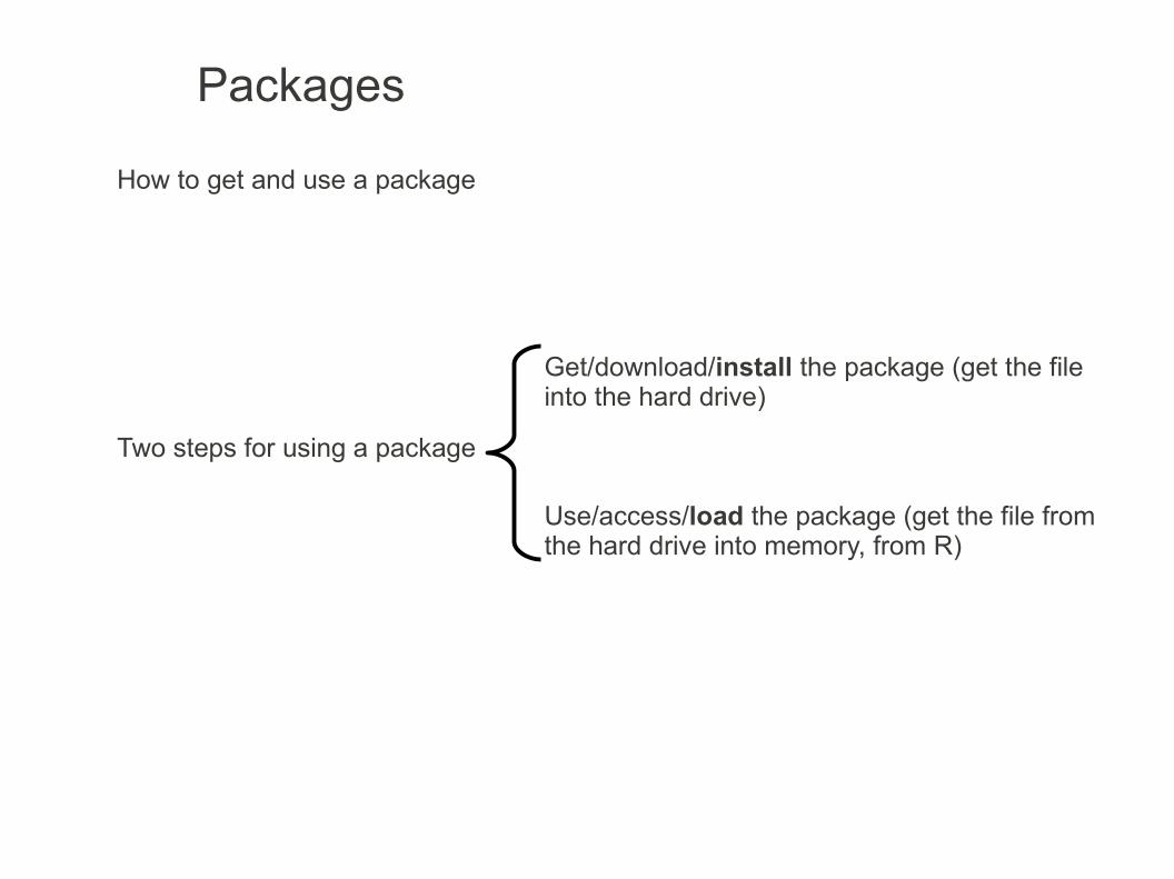
How to get and use a package
Two steps for using a package
Get/download/install the package (get the file into the hard drive)
Use/access/load the package (get the file from the hard drive into memory, from R)

Packages
Installing a package
Select repository (repositories store packages distributed by the main projects), optional
Set CRAN mirror (there are CRAN mirrors in most countries, allowing fast downloads), optional
Install package (get the file into the hard drive)Download from the web
Copy from a USB stick

Packages
Select repository
Which distributor has the necessary packages
CRAN is the basic R distribution
CRAN (extras) are Contributed R packages
BioC are packages from Bioconductor (bioinformatics/biostatistics, focused on inference using DNA microarrays)
R-forge are packages from Omegahat (umbrella project for S, R and Lisp-stats, focused on statistical tools, with web applications, web services, Java, distribuited computing, etc...)

Packages
Set CRAN mirror
Which server is closer or faster/more reliable
Sweden is the closest
Packages
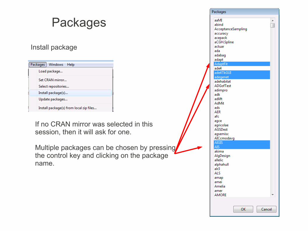
Install package
If no CRAN mirror was selected in this session, then it will ask for one.
Multiple packages can be chosen by pressing the control key and clicking on the package name.
Packages
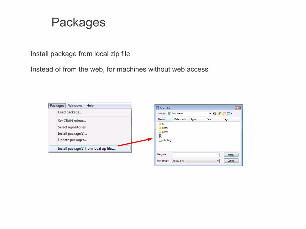
Install package from local zip file
Instead of from the web, for machines without web access

Packages
available.packagesold.packagesnew.packagesdownload.packagesupdate.packagesinstall.packagesremove.packages
Functions to work with packages
available.packages() - packages/bundles available at one or more repositories
old.packages() - packages/bundles that have newer versions on the repositories
new.packages() - uninstalled packages/bundles that are available at the repositories
download.packages() - downloads the newest versions of packages/bundles
update.packages() - the user will be prompted for which packages/bundles with a newer version to update
install.packages() - installs new packages/bundles
remove.packages() - removes installed packages/bundles and updates index information as necessary

Packages
When do I need such functions?
available.packages() - I want a list of all the existing packages!
old.packages() - are there newer versions of the packages/bundles installed?
new.packages() - are there new packages/bundles?
download.packages() - I want to download packages/bundles.
update.packages() - I want to see which packages/bundles have a newer version and decide, interactively, which ones to update.
install.packages() - I want to install packages/bundles.
remove.packages() - I want to remove installed packages/bundles.

PackagesOther functions:
library() list all available packages
library(lib.loc = .Library) list all packages in the default library
library(ada) load package "ada"
require(ada) load the package "ada" from inside other functions
library(help = ada) documentation on package 'ada'
search() list of attached packages and R objects
.packages information about package availability
.packages(all.available = TRUE) return all available as character vector
detach("package:ada") unload package "ada"
Trying to use function "foo" from a package that is not yet loaded will return an error:Error: could not find function "foo"

Packages
search() = .packages() + R objects
library() = .packages(all.available = TRUE) with description
Loaded packages
Installed packages
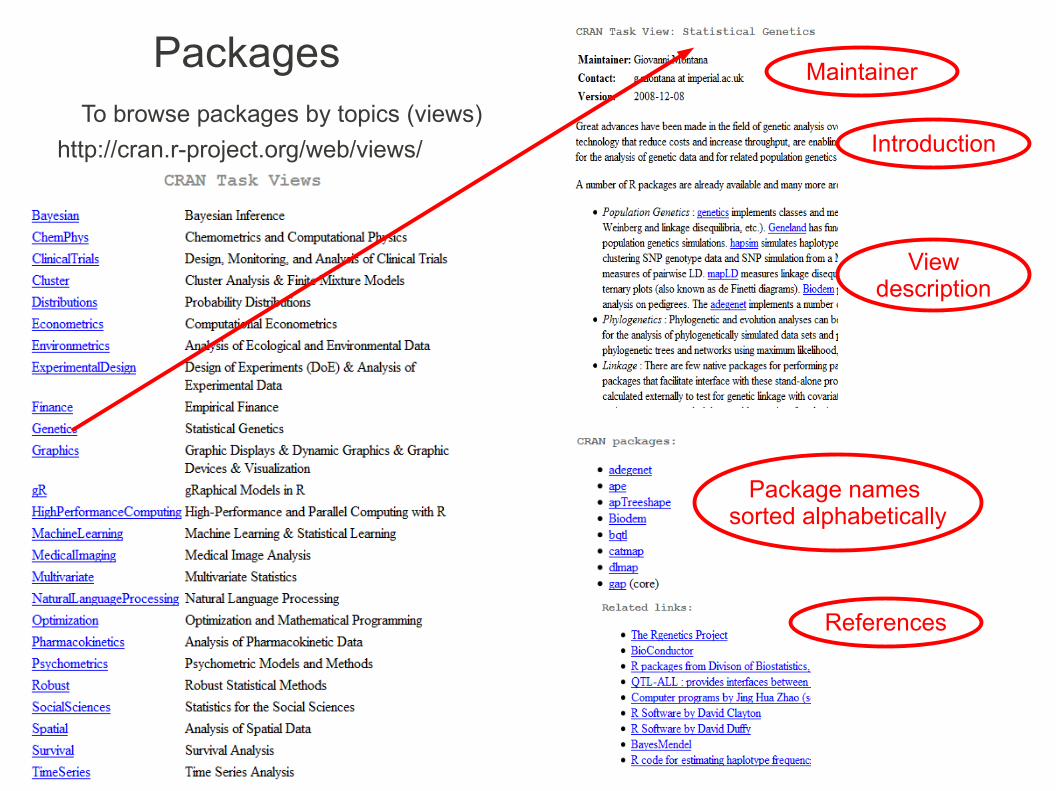
PackagesTo browse packages by topics (views)
http://cran.r-project.org/web/views/
Maintainer
Introduction
Viewdescription
Package names sorted alphabetically
References

CRAN task views are categories of contributed packages with simplified installation:
To automatically install these views, the ctv package needs to be installed:install.packages("ctv")library("ctv")
The views can be installed now:install.views("Genetics")orupdate.views("Genetics")
Packages
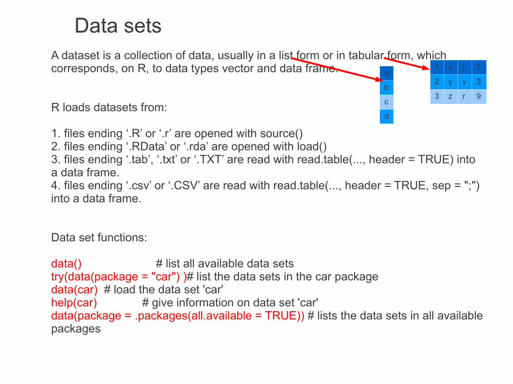
Data setsA dataset is a collection of data, usually in a list form or in tabular form, which corresponds, on R, to data types vector and data frame.
R loads datasets from:
1. files ending ‘.R’ or ‘.r’ are opened with source()2. files ending ‘.RData’ or ‘.rda’ are opened with load()3. files ending ‘.tab’, ‘.txt’ or ‘.TXT’ are read with read.table(..., header = TRUE) into a data frame.4. files ending ‘.csv’ or ‘.CSV’ are read with read.table(..., header = TRUE, sep = ";") into a data frame.
Data set functions:
data() # list all available data setstry(data(package = "car") )# list the data sets in the car packagedata(car) # load the data set 'car'help(car) # give information on data set 'car'data(package = .packages(all.available = TRUE)) # lists the data sets in all available packages
a
b
c
d
1 x j 7
2 y v 3
3 z r 9

R comes with some datasets already installed, one is pressure and it is the "Vapor Pressure of Mercury as a Function of Temperature".
require(graphics) #just to make sure the graphics library is loadedpressure?pressure
mean(pressure)median(pressure)min(pressure)max(pressure)quantile(pressure$pressure)summary(pressure)
var(pressure)sd(pressure)cor(pressure)
boxplot(pressure)
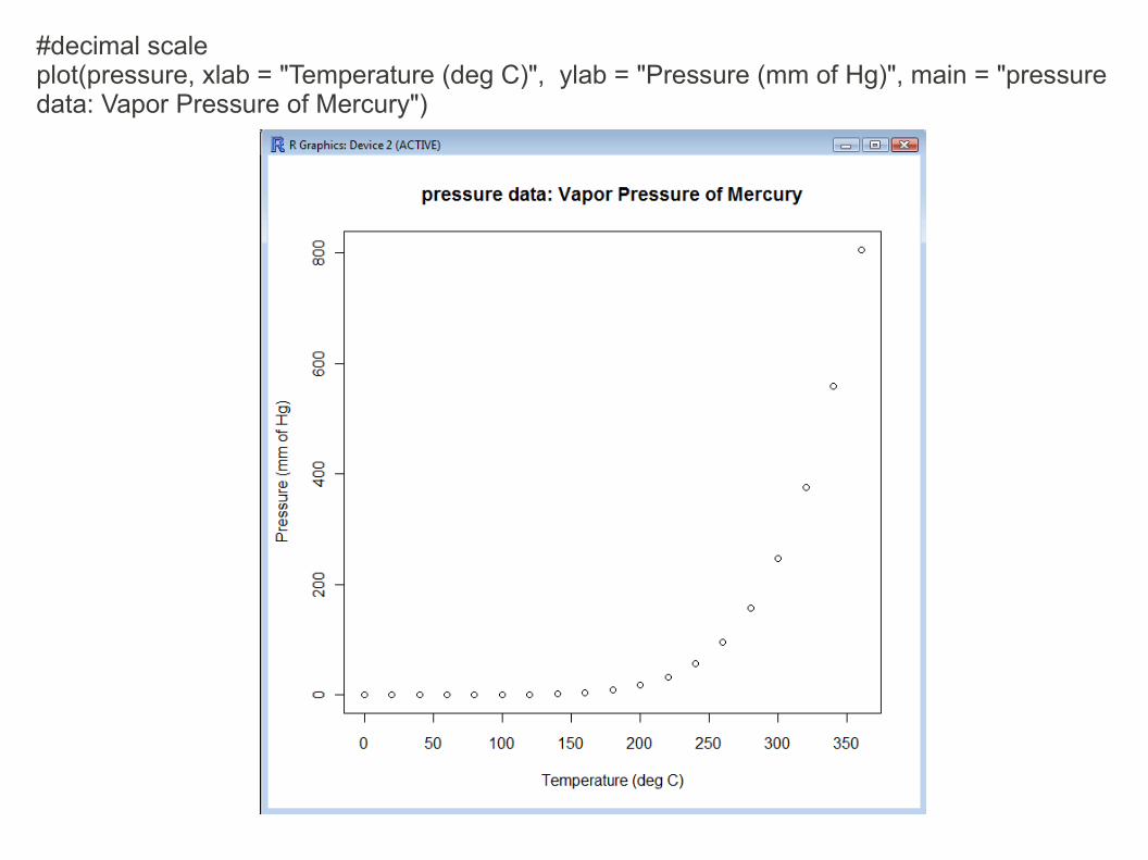
#decimal scaleplot(pressure, xlab = "Temperature (deg C)", ylab = "Pressure (mm of Hg)", main = "pressure data: Vapor Pressure of Mercury")

#log scaleplot(pressure, xlab = "Temperature (deg C)", log = "y", ylab = "Pressure (mm of Hg)", main = "pressure data: Vapor Pressure of Mercury")

Assignment: packages and help
1. Is the car package loaded?2. Is the car package installed?3. Install the car package4. Load the car package5. Is there help for the car package?6. Find out information about the data frame Angell7. Find out what the function scatterplot does8. Run an example of scatterplot9. Unload the car package10. Uninstall the car package11. List packages for epidemiology12. List packages for environmental sciences
http://cran.r-project.org/web/packages/car/car.pdf
Packages

Packages
1. Is the car package loaded?2. Is the car package installed?
> # 1. Is the car package loaded?> (.packages())[1] "stats" "graphics" "grDevices" "utils" "datasets" "methods" [7] "base" > # 2. Is the car package installed?> (.packages(all.available=TRUE)) [1] "biglm" "DBI" "ISwR" "leaps" [5] "RODBC" "RSQLite" "scatterplot3d" "base" [9] "boot" "class" "cluster" "codetools" [13] "datasets" "foreign" "graphics" "grDevices" [17] "grid" "KernSmooth" "lattice" "MASS" [21] "Matrix" "methods" "mgcv" "nlme" [25] "nnet" "rpart" "spatial" "splines" [29] "stats" "stats4" "survival" "tcltk" [33] "tools" "utils"
Packages
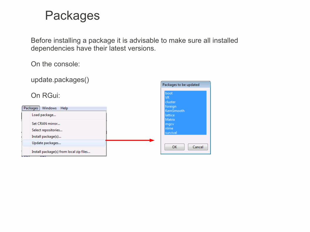
Before installing a package it is advisable to make sure all installed dependencies have their latest versions.
On the console:
update.packages()
On RGui:

Packages3. Install package carwith RGui from the web
From the console:
install.packages("car", dependencies = TRUE)

PackagesInstall package car from a zip file
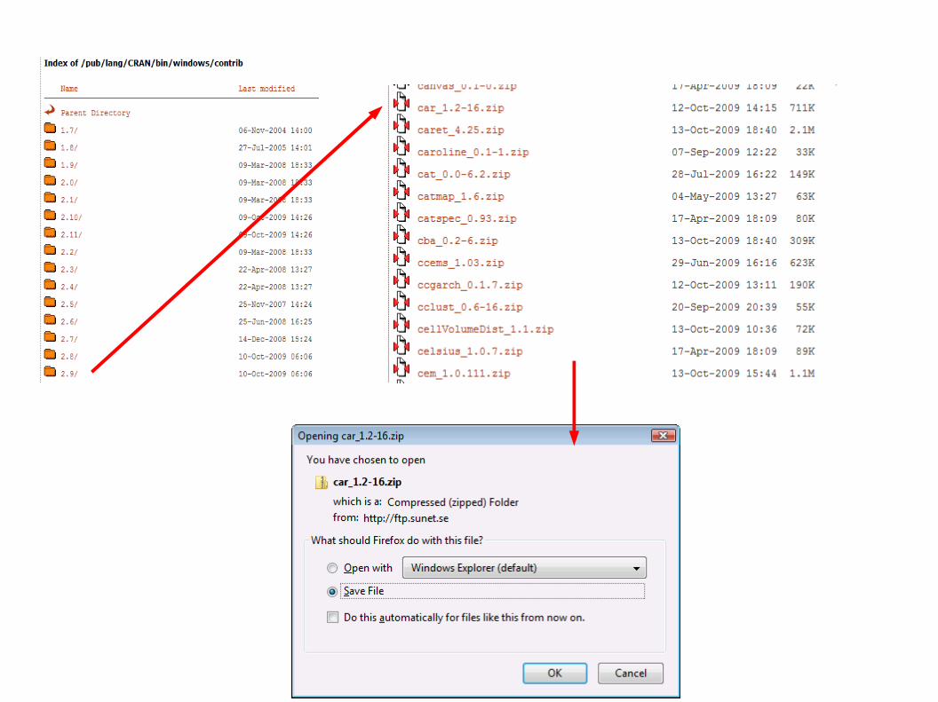

Install package car from a zip file
Copy the zip file to the working directory
Packages
From the console:
install.packages("car_1.2-16.zip")
On linux or MacOsx:
R CMD INSTALL car.tar.gz

Packages
Double check:
Is the car package loaded?Is the car package installed?
Installed

Packages
Double check:
Is the car package loaded?
4. Load the car package
Loaded

Packages
# 5. Is there help for the car package?
# 6. Find out information about the data frame Angell
library(help = car)
help(Angell)

?scatterplot
Packages7. Find out what the function scatterplot does
8. Run an example of scatterplot
scatterplot(prestige ~ income|type, data=Prestige, span=1)

Packages
9. Unload the car package10. Uninstall the car package

.libPaths() # get library locationdir(.libPaths()) # show files and directories on the library location
# 1. Is the car package loaded?# search() is the "usual" command but it it also shows R objects (unnecessary info)(.packages())# 2. Is the car package installed?# library() is the "usual" command but it it also shows the description (unnecessary info)(.packages(all.available=TRUE))
# 3. Install package car from the webinstall.packages("car", dependencies = TRUE)
# 2. Is the car package installed?(.packages(all.available=TRUE))
dir(.libPaths()) # show files and directories on the library location
# 4. Load the car packagelibrary("car")
# 1. Is the car package loaded?(.packages())
# 5. Is there help for the car package?library(help=car)
# 9. Unload the car package
# 1. Is the car package loaded?(.packages())
# 10. Uninstall the car package
# 2. Is the car package installed?(.packages(all.available=TRUE))dir(.libPaths()) # show files and directories on the library location
Internet CRANmirror
Hard drive.libPaths()
Install package car from the web
Load the car package
RMemory

Packages
11. List packages for epidemiology
12. List packages for environmental sciences
Check out BioConductor!
Look at the description of each view, Spatial has this:

Packages11. List packages for epidemiology
?? search the installed help filesFor keywords “epidem”, “disease”, “illness”, etc...
R Site Searchhttp://search.r-project.org/
Rseekhttp://www.rseek.org/
Read and maybe post a question on the Mailing ListR-help -- Main R Mailing Listhttps://stat.ethz.ch/mailman/listinfo/r-help
crantastic, a community site for R packages to search for, review and tag CRAN packages. http://crantastic.org/
sos package R related Search Enginehttp://cran.r-project.org/web/packages/sos/
Stack Overflow a programming Q & A sitehttp://stackoverflow.com/
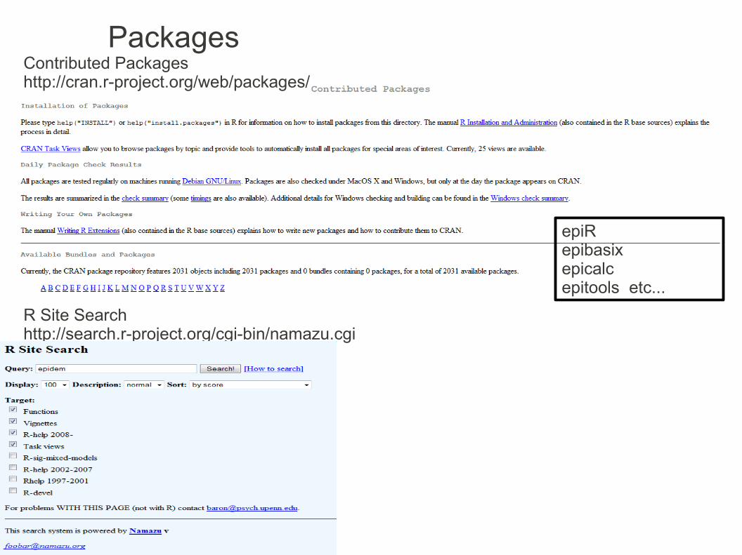
R Site Searchhttp://search.r-project.org/cgi-bin/namazu.cgi
Contributed Packageshttp://cran.r-project.org/web/packages/
epiRepibasixepicalcepitools etc...
Packages

packagesReferences/to learn more:
The R bookMichael J. Crawley pp 42009 John Wiley & Sons Ltd
Basic statistics using R pp. 16Jarno Tuimala (CSC) and Dario Greco (HY)http://www.csc.fi/english/csc/courses/archive/R2008s
Statistics with RVincent Zoonekynd, pp 115http://zoonek2.free.fr/UNIX/48_R/all.html
Introductory Statistics with RPeter Dalgaard, pp 352010 Springer
Geographic Data AnalysisPat Bartleinhttp://geography.uoregon.edu/bartlein/courses/geog417/lectures/lec05.htm
Quick-RRob Kabacoffhttp://www.statmethods.net/interface/packages.html

R console inputThe console will accept R code, functions, expressions, variables and data.
Numbers can be positive or negative, and with a decimal part.
Strings are delimited by double quotes. Strings are text, character data.
Comments are marked with the # sign. Everything after a comment is ignored. Comments are useful for explaining the code, otherwise it would be hard trying to guess or remember what the code does.
Examples:

Using R as a calculatorR can execute expressions directly from the console, like a calculator
Type 1+1 and enter
Mathematical operators

Using R as a calculator
Comparison operators
The logical values are TRUE, FALSE and NA for missing values.

Using R as a calculatorLogical operators
The logical values are TRUE, FALSE and NA for missing values.
> !FALSE # logical negation[1] TRUE> TRUE & FALSE # logical AND[1] FALSE> TRUE | FALSE # logical OR[1] TRUE> xor(TRUE, FALSE) # logical eXclusive OR[1] TRUE> > TRUE && FALSE # logical AND[1] FALSE> TRUE || FALSE # logical OR[1] TRUE> > c(T,F,F) & c(F,T,F) # logical AND[1] FALSE FALSE FALSE> c(T,F,F) | c(F,T,F) # logical OR[1] TRUE TRUE FALSE> c(T,F,F) && c(F,T,F) # logical AND[1] FALSE> c(T,F,F) || c(F,T,F) # logical OR[1] TRUE

Using R as a calculator
Rounding functions

Using R as a calculator
Mathematical functions
Using R as a calculator
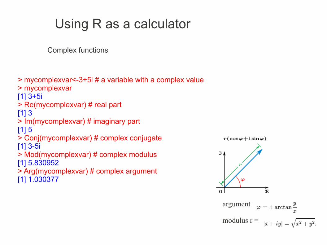
Complex functions
> mycomplexvar<-3+5i # a variable with a complex value> mycomplexvar[1] 3+5i> Re(mycomplexvar) # real part[1] 3> Im(mycomplexvar) # imaginary part[1] 5> Conj(mycomplexvar) # complex conjugate[1] 3-5i> Mod(mycomplexvar) # complex modulus[1] 5.830952> Arg(mycomplexvar) # complex argument[1] 1.030377
argument
modulus r =

R Built-in Constants
Constants that come with the R base package.
LETTERS: the 26 upper-case letters of the Roman alphabet; letters: the 26 lower-case letters of the Roman alphabet; month.abb: the three-letter abbreviations for the English month names; month.name: the English names for the months of the year; pi: the ratio of the circumference of a circle to its diameter.
pi * 10 # the perimeter of a circumference of diameter 10
# months in Englishmonth.name# months in your current localeformat(ISOdate(2009, 1:12, 1), "%B")format(ISOdate(2009, 1:12, 1), "%b")
Using R as a calculator

R as calculatorReferences/to learn more:
The R bookMichael J. Crawley pp 92010 John Wiley & Sons Ltd
Basic statistics using R pp. 35Jarno Tuimala (CSC) and Dario Greco (HY)http://www.csc.fi/english/csc/courses/archive/R2008s
Statistics: an introduction using RMichael J. Crawley pp 2812008 John Wiley & Sons Ltd
Aprendizaje del software estadístico R: un entorno para simulación y computación estadísticaProf. Alberto muñoz garcíaDepartamento de EstadísticaUniversidad Carlos III de Madridhttp://ocw.uc3m.es/estadistica/aprendizaje-del-software-estadistico-r-un-entorno-para-simulacion-y-computacion-estadistica/resolveUid/6bfdf37a91c966902de8395629e9fef6
Introductory Statistics with RPeter Dalgaard, pp 32011 Springer
Software Tools, Part 1: introduction to R softwarePetri Koistinenhttp://www.rni.helsinki.fi/~pek/s-tools/calculator.r

Assigning values to objects = or <- or ->
R Variables
> myvar <- 123 # to assign value 123 to variable "myvar"> print(myvar) # display the variable[1] 123> #or> myvar[1] 123> x = 5> y <- 6> 7 -> z> x[1] 5> y[1] 6> z[1] 7> (myvar2 <- 456) # assign and display[1] 456
> a <- b <- 55> a[1] 55> b[1] 55> > x <- (y <- c(5, 14,234))*2> x;y[1] 10 28 468[1] 5 14 234
Multiple commands in one line
Multiple assignments

R Variables
3 basic types of variables
Numeric
Character
Boolean {true, false}
Functions to test an object's data type
is.integer, is.double, is.numeric, is.character and is.logical
as.integer is used to pass data to C or Fortran code

R Variables
Variable names
●Case sensitive●R names depend on the operating system and country within which R is being run (technically on the locale settings)●All alphanumeric symbols are allowed (and in some countries this includes accented letters) plus ‘.’ and ‘_’, with the restriction that a name must start with ‘.’ or a letter, and if it starts with ‘.’ the second character must not be a digit●For portable R code (including that to be used in R packages) use only A–Za–z0–9
Although legal,these variable names
are confusing
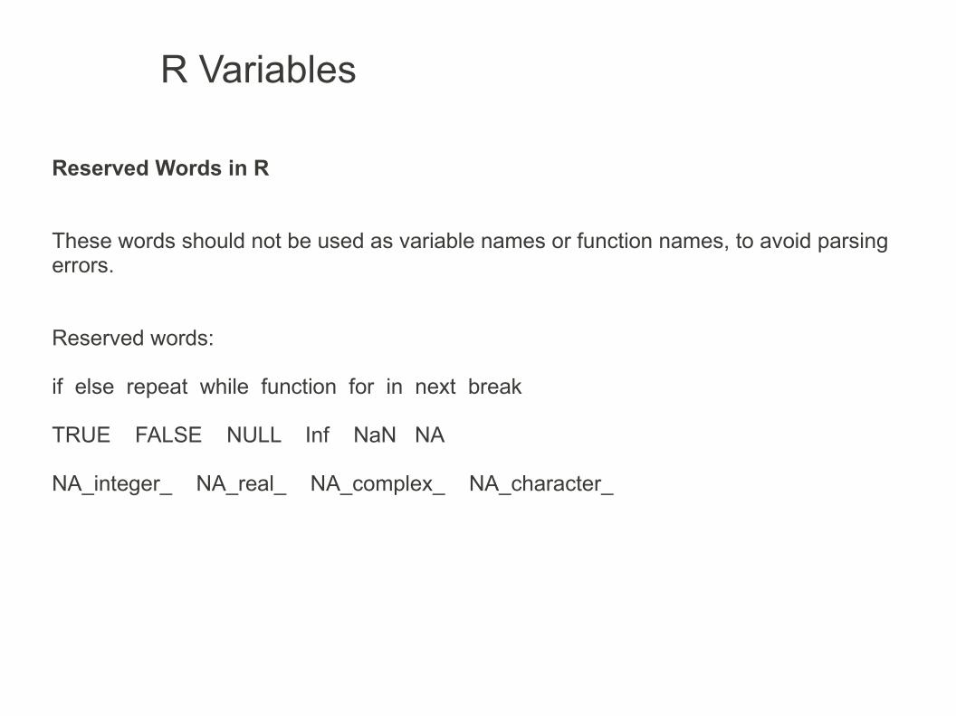
Reserved Words in R
These words should not be used as variable names or function names, to avoid parsing errors.
Reserved words:
if else repeat while function for in next break
TRUE FALSE NULL Inf NaN NA
NA_integer_ NA_real_ NA_complex_ NA_character_
R Variables

Not Available / "Missing" Values
NA is a missing value indicator.
"Missing" Values are common in real world data because of no answers to surveys or missing data from sensors readings.
is.na() returns TRUE for missing elementsis.na() <- sets elements to NA
> x <- 5> x[1] 5> is.na(x)[1] FALSE> y <- NA> y[1] NA> is.na(y)[1] TRUE
R Variables

R Variables
Not Available / "Missing" Values
> z <- c(3,5,NA,6,7,8) # vector> z[1] 3 5 NA 6 7 8> is.na(z) # which elements are NA[1] FALSE FALSE TRUE FALSE FALSE FALSE> is.na(z) <- c(1,5) # turn elements at position 1 and position 5 to NA> z[1] NA 5 NA 6 NA 8
> # math operators * + - / will return NA> 5 * NA[1] NA
> # comparison operators < <= > >= == != will return NA> c(5, 5, NA) == c(5, NA, NA)[1] TRUE NA NA

R Variables
Not Available / "Missing" Values
> # NA is "undetermined" for logical expressions> c(T, F) & c(NA, NA) # FALSE AND whatever is FALSE[1] NA FALSE> c(T, F) | c(NA, NA) # TRUE OR whatever is TRUE[1] TRUE NA> xor(NA,T)[1] NA
> myvec <- c(7,4,NA,2,65)> mean(myvec) # this will return NA[1] NA> mean(myvec, na.rm=T) # ignoring NA in a calculation[1] 19.5> na.omit(myvec) # omitting NA[1] 7 4 2 65attr(,"na.action")[1] 3attr(,"class")[1] "omit"

R Variables
> x <- c(7, 6, NA, NA, 5)> x[!is.na(x)] # get the data except the NAs[1] 7 6 5> na.omit(x) # get the data except the NAs, proper way[1] 7 6 5attr(,"na.action")[1] 3 4attr(,"class")[1] "omit"> mean(x) # returns NA[1] NA> mean(x, na.rm=TRUE) # returns 6 [1] 6> x[is.na(x)] <- 0 # replace NAs with 0> x[1] 7 6 0 0 5

http://www.khpa.ks.gov/data_consortium/Docs/022009/WorkForceSurvey.pdf

Missing image data LANDSAT 5 - 7
Anomalies descriptionMissing image data anomaly may be considered under different aspects. The most frequently case ofmissing data may be called “missing pixels”. Usually, the “missing pixels” anomaly is correlated withothers anomalies (shifted swath – speckle - missing swath). Details are also provided about wrong ormissing auxiliary data that implies swath misalignment (See also Anomaly slip 02). This section describesthe following anomalies related to missing image data:· Missing pixels.· Missing pixels – shifted swath.· Missing pixels – missing swath.· Missing pixels – speckle.· Corrupted Mirror Scan Correction Data (MSCD) – shifted swath.
http://earth.esa.int/pub/ESA_DOC/landsat_product_anomalies/GAEL-P157-SLP-001-03-01.pdf

NA
http://www.ktl.fi/attachments/suomi/julkaisut/julkaisusarja_b/2004b13.pdf

http://www.woodrow.org/teachers/ci/1992/activities/birthdays.html
Using data from a website:
NA
The data is clean and organized on a spreadsheet:
NA
<td>1</td><td>Eugene A. Demarcay, 1852<br></td></tr><tr><td> 2</td><td>Roger Adams, 1889<br>Charles Hatchett, 1765<br>Rudolph Clausius, 1822<br></td></tr><tr><td>4</td><td>Astrid V. Grosse, 1905<br>Joseph Elanger, 1874<br>
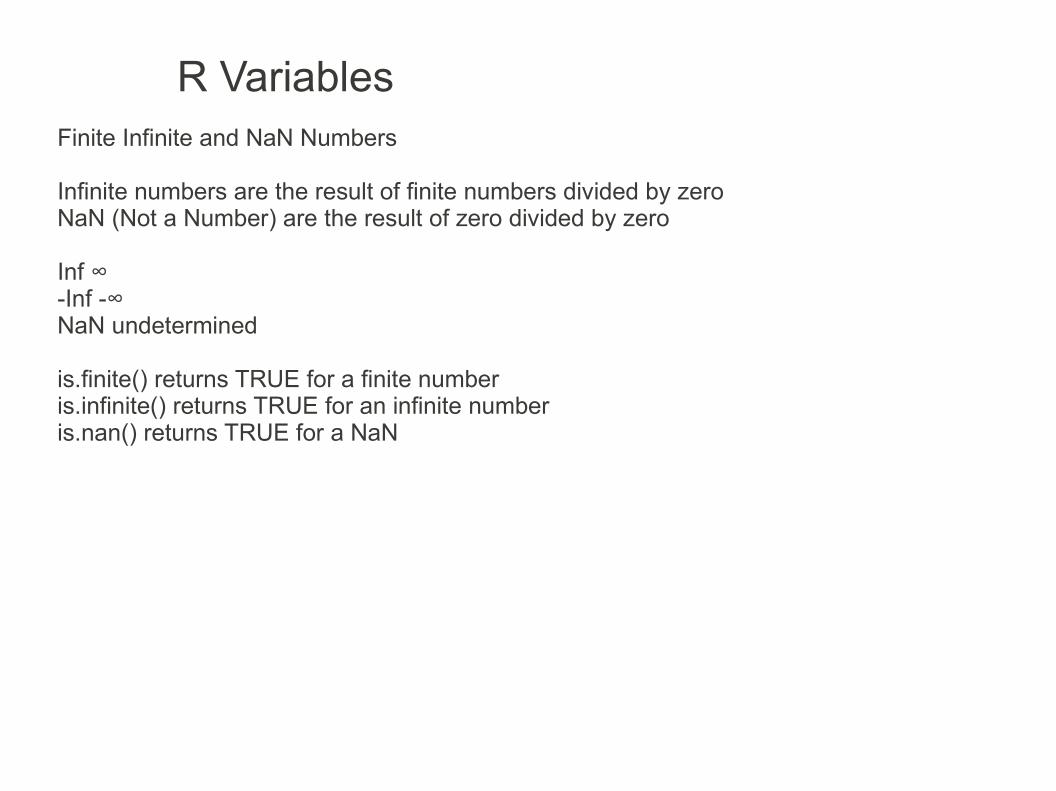
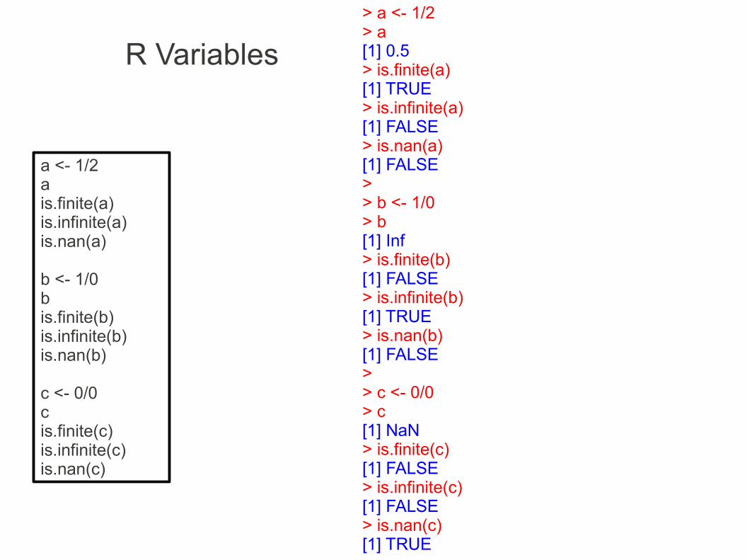
R VariablesFinite Infinite and NaN Numbers
Infinite numbers are the result of finite numbers divided by zeroNaN (Not a Number) are the result of zero divided by zero
Inf ∞-Inf -∞NaN undetermined
is.finite() returns TRUE for a finite numberis.infinite() returns TRUE for an infinite numberis.nan() returns TRUE for a NaN
R Variables
> a <- 1/2> a[1] 0.5> is.finite(a)[1] TRUE> is.infinite(a)[1] FALSE> is.nan(a)[1] FALSE> > b <- 1/0> b[1] Inf> is.finite(b)[1] FALSE> is.infinite(b)[1] TRUE> is.nan(b)[1] FALSE> > c <- 0/0> c[1] NaN> is.finite(c)[1] FALSE> is.infinite(c)[1] FALSE> is.nan(c)[1] TRUE
a <- 1/2ais.finite(a)is.infinite(a)is.nan(a)
b <- 1/0bis.finite(b)is.infinite(b)is.nan(b)
c <- 0/0cis.finite(c)is.infinite(c)is.nan(c)

R VariablesGetting info from objects
class() returns the class attribute or the implicit class of this object
is() returns all the super-classes of this object's class
mode() to get or set the type or storage mode of an object
str() to compactly display the internal structure of an R object
length() to get or set the length of objects
dim() to retrieve or set the dimension of an object
nchar() to get or set the length of strings
object.size() to get an estimate of the memory used to store an R object
Common source of confusion:
class() vs is() vs mode()
length() vs dim() vs nchar()

R VariablesType on R Editor:
Myint <- 567is(myint)Myreal <- 8.83is(myreal)mycomplex <- 34-7iis(mycomplex)mystring <- "quartz"is(mystring)myvector_i <- c(6,5,4)is(myvector_i)myvector_s <- c("a","b","c")is(myvector_s)mymatrix <- matrix(5,2,3)is(mymatrix)

R Variables
> myint <- 567> is(myint)[1] "numeric" "vector" > myreal <- 8.83> is(myreal)[1] "numeric" "vector" > mycomplex <- 34-7i> is(mycomplex)[1] "complex" "vector" > > mystring <- "quartz"> is(mystring)[1] "character" "vector" "data.frameRowLabels"> myvector_i <- c(6,5,4)> is(myvector_i)[1] "numeric" "vector" > > myvector_s <- c("a","b","c")> is(myvector_s)[1] "character" "vector" "data.frameRowLabels"> mymatrix <- matrix(5,2,3)> is(mymatrix)[1] "matrix" "array" "structure" "vector"
All objects are vectors!
Scalars are vectors of length 1
is() returns all the super-classes of this object's class

R VariablesOn R Editor, go to Edit/Replace and replace “is” with “class”
myint <- 567class(myint)myreal <- 8.83class(myreal)mycomplex <- 34-7iclass(mycomplex)mystring <- "quartz"class(mystring)myvector_i <- c(6,5,4)class(myvector_i)myvector_s <- c("a","b","c")class(myvector_s)mymatrix <- matrix(5,2,3)class(mymatrix)
Edit/Clear console to clear the previous calculations from the R Console

R Variables
> myint <- 567> class(myint)[1] "numeric"> myreal <- 8.83> class(myreal)[1] "numeric"> mycomplex <- 34-7i> class(mycomplex)[1] "complex"> mystring <- "quartz"> class(mystring)[1] "character"> myvector_i <- c(6,5,4)> class(myvector_i)[1] "numeric"> myvector_s <- c("a","b","c")> class(myvector_s)[1] "character"> mymatrix <- matrix(5,2,3)> class(mymatrix)[1] "matrix"
class() returns the class attribute or the implicit class of this object
This is the first class returned by is()
class(myvar) "class 1"
is(myvar) "class 1" "class 2" "class 3" ...

R VariablesOn R Editor, go to Edit/Replace and replace “class” with “mode”
myint <- 567mode(myint)myreal <- 8.83mode(myreal)mycomplex <- 34-7imode(mycomplex)mystring <- "quartz"mode(mystring)myvector_i <- c(6,5,4)mode(myvector_i)myvector_s <- c("a","b","c")mode(myvector_s)mymatrix <- matrix(5,2,3)mode(mymatrix)

mode() to get or set the type or storage mode of an object
R Variables
> myint <- 567> mode(myint)[1] "numeric"> myreal <- 8.83> mode(myreal)[1] "numeric"> mycomplex <- 34-7i> mode(mycomplex)[1] "complex"> mystring <- "quartz"> mode(mystring)[1] "character"> myvector_i <- c(6,5,4)> mode(myvector_i)[1] "numeric"> myvector_s <- c("a","b","c")> mode(myvector_s)[1] "character"> mymatrix <- matrix(5,2,3)> mode(mymatrix)[1] "numeric"
The only difference is with matrix, let's try a data frame:
> mydataf <- data.frame(1,2,3)> mode(mydataf)[1] "list"> class(mydataf)[1] "data.frame"> mydataf <- data.frame("a","b","c")> mode(mydataf)[1] "list"> class(mydataf)[1] "data.frame"
By default, a matrix is stored as numeric data in memory and a data frame as list data in memory. This can be changed, for achieving better performance or for compatibility.

R VariablesOn R Editor, go to Edit/Replace and replace “mode” with “length”, “dim” and “nchar”
myint <- 567length(myint)myreal <- 8.83length(myreal)mycomplex <- 34-7ilength(mycomplex)mystring <- "quartz"length(mystring)myvector_i <- c(6,5,4)length(myvector_i)myvector_s <- c("a","b","c")length(myvector_s)mymatrix <- matrix(5,2,3)length(mymatrix)
myint <- 567dim(myint)myreal <- 8.83dim(myreal)mycomplex <- 34-7idim(mycomplex)mystring <- "quartz"dim(mystring)myvector_i <- c(6,5,4)dim(myvector_i)myvector_s <- c("a","b","c")dim(myvector_s)mymatrix <- matrix(5,2,3)dim(mymatrix)
myint <- 567nchar(myint)myreal <- 8.83nchar(myreal)mycomplex <- 34-7inchar(mycomplex)mystring <- "quartz"nchar(mystring)myvector_i <- c(6,5,4)nchar(myvector_i)myvector_s <- c("a","b","c")nchar(myvector_s)mymatrix <- matrix(5,2,3)nchar(mymatrix)

R Variables
> myint <- 567> length(myint)[1] 1> myreal <- 8.83> length(myreal)[1] 1> mycomplex <- 34-7i> length(mycomplex)[1] 1> mystring <- "quartz"> length(mystring)[1] 1> myvector_i <- c(6,5,4)> length(myvector_i)[1] 3> myvector_s <- c("a","b","c")> length(myvector_s)[1] 3> mymatrix <- matrix(5,2,3)> length(mymatrix)[1] 6
> myint <- 567> dim(myint)NULL> myreal <- 8.83> dim(myreal)NULL> mycomplex <- 34-7i> dim(mycomplex)NULL> mystring <- "quartz"> dim(mystring)NULL> myvector_i <- c(6,5,4)> dim(myvector_i)NULL> myvector_s <- c("a","b","c")> dim(myvector_s)NULL> mymatrix <- matrix(5,2,3)> dim(mymatrix)[1] 2 3
> myint <- 567> nchar(myint)[1] 3> myreal <- 8.83> nchar(myreal)[1] 4> mycomplex <- 34-7i> nchar(mycomplex)[1] 5> mystring <- "quartz"> nchar(mystring)[1] 6> myvector_i <- c(6,5,4)> nchar(myvector_i)[1] 1 1 1> myvector_s <- c("a","b","c")> nchar(myvector_s)[1] 1 1 1> mymatrix <- matrix(5,2,3)> nchar(mymatrix) [,1] [,2] [,3][1,] 1 1 1[2,] 1 1 1
Length() is the number of elements, dim are the dimensions, nchar is the number of characters

Quitting RCommand q()
Or File/Exit or close the editor window (on Windows)
save workspace image?
Yes will save all the objects from memory to a file .Rdata and it wil also save all the commands typed during the session to a file .Rhistory
Both files are saved on user\documents
The file .Rhistory is plain text and it can be examined or edited.
To close R without the question:q(save = "no")

R's workspace
R can save all the objects from memory to a file .Rdata and save all the commands typed during the session to a file .Rhistory, these are the default file names and they are saved on the working directory
Once a workspace is saved, it will be automatically loaded:
By changing the working directory, many default workspace files can be used, on different directories.
But, the next session will open the default workspace, on the default working directory.
R's workspace
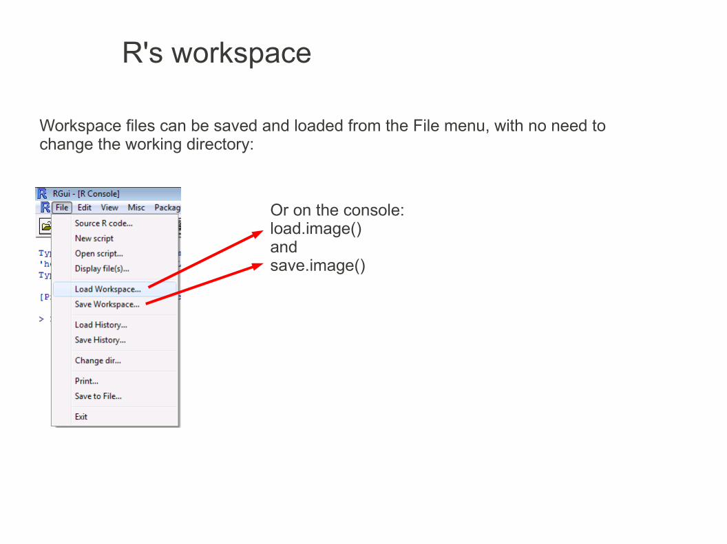
Workspace files can be saved and loaded from the File menu, with no need to change the working directory:
Or on the console:load.image()andsave.image()

R's workspace
shows the contents of the workspace, sames as objects() or ls()
clears the workspace, sames as rm(list = ls(all = TRUE))
list of attached packages and R objects, sames as search()
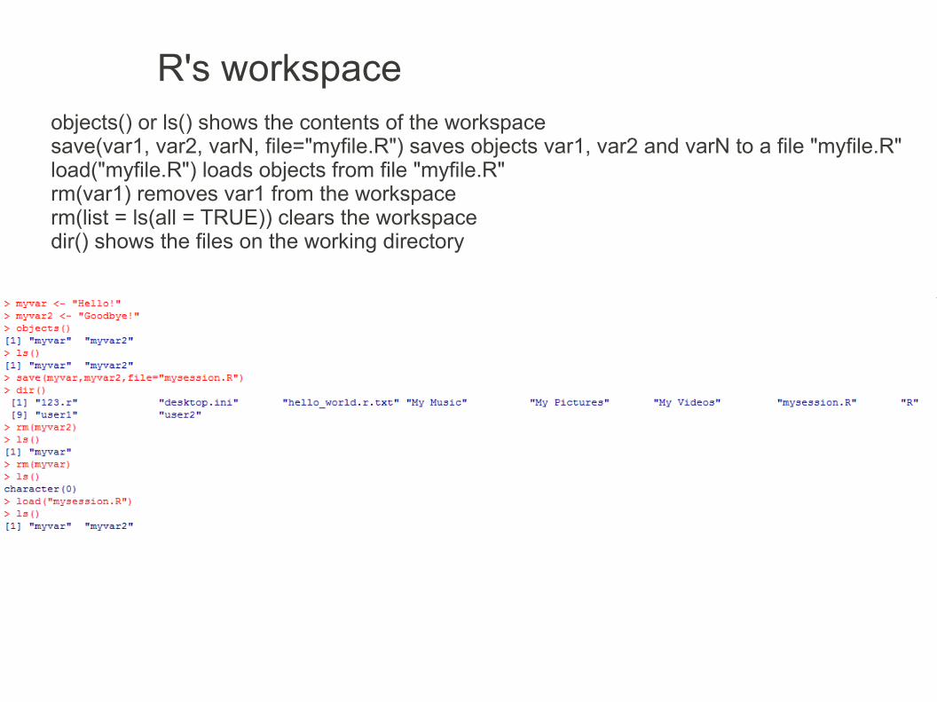
R's workspaceobjects() or ls() shows the contents of the workspacesave(var1, var2, varN, file="myfile.R") saves objects var1, var2 and varN to a file "myfile.R"load("myfile.R") loads objects from file "myfile.R"rm(var1) removes var1 from the workspacerm(list = ls(all = TRUE)) clears the workspacedir() shows the files on the working directory

R's working directory
Working DirectoryDefault setting on Linux is $R_HOME\binDefault setting on Windows is C:/Users/MyUserName/Documents
The command "system" executes OS commands
> getwd() # get the working directory[1] "C:/Users/user/Documents"> setwd("C:/Users/user/Documents/test123") # change the working directoryError in setwd("C:/Users/user/Documents/test123") : cannot change working directory> getwd() # it didn't change because the directory does not exist[1] "C:/Users/user/Documents"> system("md test123") # create a directory on LinuxWarning message:In system("md test123") : md not found> system(paste(Sys.getenv("COMSPEC"),"/c", "md test123")) # create a directory on Windows> setwd("C:/Users/user/Documents/test123")> getwd()[1] "C:/Users/user/Documents/test123"

getwd()myvar1 <- "variable 1 is a string"myvar2 <- -2342.452dir()dir(all.files = T)savehistory() # save the command history to the default file (.Rhistory)save.image() # save the workspace to the default file (.RData)dir() # it won't show .Rhistory and .RDatadir(all.files = T) # now it shows all the files!file.show(".Rhistory") # display the history file, a text file is okfile.show(".RData") # a binary data can't be displayed
R's working directory and workspace

Creating a shortcut on the desktop to the working directory
R's working directory
On Windows explorer, right click on the working directory and choose “Send To”, then choose “Desktop (create shortcut)”

programming R workspaceReferences/to learn more:
Basic statistics using R pp. 76Jarno Tuimala (CSC) and Dario Greco (HY)http://www.csc.fi/english/csc/courses/archive/R2008s
Aprendizaje del software estadístico R: un entorno para simulación y computación estadísticaProf. Alberto muñoz garcíaDepartamento de EstadísticaUniversidad Carlos III de Madridhttp://ocw.uc3m.es/estadistica/aprendizaje-del-software-estadistico-r-un-entorno-para-simulacion-y-computacion-estadistica/resolveUid/a70c8973cb8798b0bd0e6bdf7abd6ec7
Introductory Statistics with RPeter Dalgaard, pp 312012 Springer
Quick-RRob Kabacoffhttp://www.statmethods.net/interface/workspace.html

Data Structures in R
All objects are vectors
there are five other classesfor the basic data structures
Factor
Matrix
Array
Dataframe
list

Data Structures in R
3 types of vectors
Numeric
Character
Boolean {true, false}
A vector is a dynamic array, that is, a unidimensional array that can be resized and allows elements to be added or removed.
Vector elements are numbered from 1 to n, n is the size of the vector. Elements can be accessed through their index with square brackets [ ], negative indeces = exclusion
4 ways to create vectors
: - colon operator
c() - "concatenate" function
seq() - "sequence" function
rep() - repetition function
> c(734, 985, 43, 952)[1] 734 985 43 952> c("Helsinki","Tampere","Turku")[1] "Helsinki" "Tampere" "Turku" > c(T,F,F,F,T,F,T,F,T,T) [1] TRUE FALSE FALSE FALSE TRUE FALSE TRUE FALSE TRUE TRUE
a
b
c
d
Vector

Data Structures in R: - colon operator
Generates regular sequences from a starting value of the sequence to an end value of the sequence. The values are either a number (numeric or integer) or a factor.The first element is from and the next ones' are from plus or minus one, up to or down to to.
Syntax:from:to
The increment is always 1 or -1 for numeric arguments.If from is integer then the result is integer, regardless of to.
from:to is equivalent to seq(from, to)
> 2:5 # sequence of numbers from 2 to 5[1] 2 3 4 5> 5:2 # sequence of numbers from 5 down to 2[1] 5 4 3 2> -3:4 # sequence of numbers from -3 to 4[1] -3 -2 -1 0 1 2 3 4> 0:pi # sequence of numbers from 0 to π[1] 0 1 2 3> pi:7 # sequence of numbers from π to 7[1] 3.141593 4.141593 5.141593 6.141593
F(n+1) = F(n) + 1orF(n+1) = F(n) - 1
N integer implies F(n) integerN real implies F(n) real
Data Structures in R
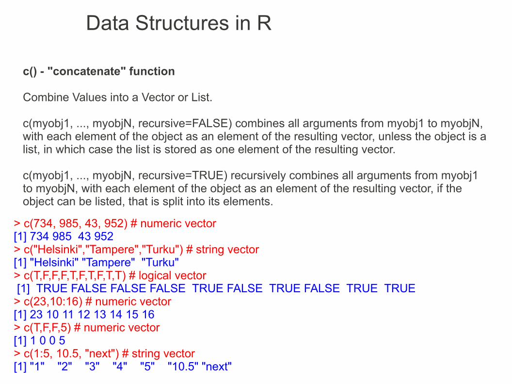
c() - "concatenate" function
Combine Values into a Vector or List.
c(myobj1, ..., myobjN, recursive=FALSE) combines all arguments from myobj1 to myobjN, with each element of the object as an element of the resulting vector, unless the object is a list, in which case the list is stored as one element of the resulting vector.
c(myobj1, ..., myobjN, recursive=TRUE) recursively combines all arguments from myobj1 to myobjN, with each element of the object as an element of the resulting vector, if the object can be listed, that is split into its elements.
> c(734, 985, 43, 952) # numeric vector[1] 734 985 43 952> c("Helsinki","Tampere","Turku") # string vector[1] "Helsinki" "Tampere" "Turku" > c(T,F,F,F,T,F,T,F,T,T) # logical vector [1] TRUE FALSE FALSE FALSE TRUE FALSE TRUE FALSE TRUE TRUE> c(23,10:16) # numeric vector[1] 23 10 11 12 13 14 15 16> c(T,F,F,5) # numeric vector[1] 1 0 0 5> c(1:5, 10.5, "next") # string vector[1] "1" "2" "3" "4" "5" "10.5" "next"

Data Structures in R
The elements of a vectors are of one data type only (Boolean, Numeric or Character) and mixing data types results in automatic data conversion. Order of conversion: boolean numeric character
> c(T,F,F,55) # boolean becomes numeric[1] 1 0 0 55> c(TRUE, FALSE, F, "Turku") # boolean becomes character[1] "TRUE" "FALSE" "FALSE" "Turku"> c(734, 985, "Turku") # numeric becomes character[1] "734" "985" "Turku"> c(TRUE, FALSE, F, T, -7.34, 72+9i, "Turku") # boolean and numeric become character[1] "TRUE" "FALSE" "FALSE" "TRUE" "-7.34" "72+9i" "Turku"

Data Structures in Rseq - "sequence" function
Generate regular sequences:seq(from = 1, to = 1, by = ((to - from)/(length.out - 1)), length.out = NULL, along.with = NULL, ...)
Arguments... arguments passed to or from methods. from, to the starting and (maximal) end value of the sequence. by number: increment of the sequence. length.out desired length of the sequence. A non-negative number, which for seq and seq.int will be rounded up if fractional. along.with take the length from the length of this argument.
> seq(4, 9) # same as 4:9[1] 4 5 6 7 8 9> seq(1,10, by= 3) # numbers starting at 1, incrementing by 3, up to 10[1] 1 4 7 10> seq(1,15, length.out= 6) # 6 numbers evenly spaced between 1 and 15[1] 1.0 3.8 6.6 9.4 12.2 15.0> seq(along.with= 4:8) # the length of this argument will be the length of the output[1] 1 2 3 4 5> seq(7) # same as 1:7[1] 1 2 3 4 5 6 7> seq(length.out= 7) # same as 1:7[1] 1 2 3 4 5 6 7> seq(1,by=3, length.out= 9) # 9 numbers, starting in 1, incremented by 3[1] 1 4 7 10 13 16 19 22 25
F(n+1) = F(n) + 1, F(n) [4, 9]
F(n+1) = F(n) + 3, F(n) [1, 10] the result is between 1 and 10
F(n+1) = F(n) + x, F(n) [1, 15] x = (15-1)/(6-1)

Data Structures in R
rep() - repetition function
Replicate elements of vectors and lists
rep(x, times, length.out, each)
Argumentsx is a scalar, a vector (including a list) or a pairlist or a factor... further arguments: times - a scalar or vector with the number of times repeat each element if times has the same length as the input, or to repeat the whole vector if times has length 1length.out - an integer with the length of the resulteach - an integer with the number of times each element of the input will be repeated
rep(x, times=1, length.out=NA, each=1) this is the default action

Data Structures in R
rep() - repetition function
> rep(14,3) # repeat number 14, 3 times[1] 14 14 14> rep(c(8,3,7),1:3) # repeat number 8, once, number 3, twice and number 7, thrice[1] 8 3 3 7 7 7> rep(c(8,3,7),1:3,4) # repeat number 8, 3 and 7 but limit the result to 4 elements[1] 8 3 7 8> rep(c(8,3,7),each=3) # repeat number 8, number 3 and number 7, thrice[1] 8 8 8 3 3 3 7 7 7> rep(c(8,3,7), length.out=7,each=3) # repeat number 8, number 3 and number 7, thrice - but limit the result to 7 elements[1] 8 8 8 3 3 3 7> rep(c(8,3,7), times=2,each=3) # repeat number 8, number 3 and number 7, thrice - do this twice [1] 8 8 8 3 3 3 7 7 7 8 8 8 3 3 3 7 7 7> rep(c(8,3,7), times=2,length.out=15,each=3) # repeat number 8, number 3 and number 7, thrice - do this twice and limit the result to 15 elements [1] 8 8 8 3 3 3 7 7 7 8 8 8 3 3 3

Data Structures in Rrep(14,3) # repeat number 14, 3 timesrep(14,4)rep(14,5)
rep(c(8,3,7),1:3) # repeat number 8, once, number 3, twice and number 7, thricerep(c(8,3,7),2:4)rep(c(8,3,7),3:5)
rep(c(8,3,7),1:3,4) # repeat number 8, 3, and 7 but limit the result to 4 elementsrep(c(8,3,7),1:3,5)rep(c(8,3,7),1:3,6)
rep(c(8,3,7),each=3) # repeat number 8, number 3 and number 7, thricerep(c(8,3,7),each=4)rep(c(8,3,7),each=5)
rep(c(8,3,7), length.out=7,each=3) # repeat number 8, number 3 and number 7, thrice - but limit the result to 7 elementsrep(c(8,3,7), length.out=8,each=3)rep(c(8,3,7), length.out=9,each=3)
rep(c(8,3,7), times=2,each=3) # repeat number 8, number 3 and number 7, thrice - do this twicerep(c(8,3,7), times=3,each=3)rep(c(8,3,7), times=4,each=3)

Data Structures in R
3 ways to extract vector elements
By the element index(es)
By a logical expression
By keys
Extracting vector elements, or subsets
a
b
c
d
myvector
1234
Indices values
On vector "myvector"Element 1 has value "a"
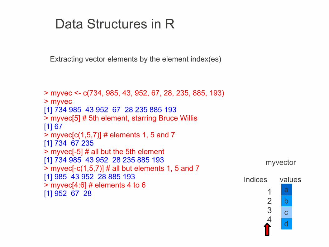
> myvec <- c(734, 985, 43, 952, 67, 28, 235, 885, 193)> myvec[1] 734 985 43 952 67 28 235 885 193> myvec[5] # 5th element, starring Bruce Willis[1] 67> myvec[c(1,5,7)] # elements 1, 5 and 7[1] 734 67 235> myvec[-5] # all but the 5th element[1] 734 985 43 952 28 235 885 193> myvec[-c(1,5,7)] # all but elements 1, 5 and 7[1] 985 43 952 28 885 193> myvec[4:6] # elements 4 to 6[1] 952 67 28
Extracting vector elements by the element index(es)
Data Structures in R
a
b
c
d
myvector
1234
Indices values

Data Structures in R
Extracting vector elements by a logical expression
The elements are selected by their value, regardless of their index
> myvec <- c(734, 985, 43, 952, 67, 28, 235, 885, 193)> myvec[1] 734 985 43 952 67 28 235 885 193> myvec[myvec > 500] # only elements above 500[1] 734 985 952 885> myvec[(myvec %% 2)==0] # only even elements[1] 734 952 28> myvec[myvec %in% 100:500] # elements with values from 100 to 500[1] 235 193
a
b
c
d
myvector
1234
Indices values

Data Structures in R
Extracting vector elements by keys
A key (name) can be used to access the vector's elements
The comand names() will add names to an existing vector, or they can be defined when creating the vector
> myvec <- c(734, 985, 43)> myvec[1] 734 985 43> names(myvec) <- c("Helsinki","Tampere","Turku")> myvecHelsinki Tampere Turku 734 985 43 > myvec["Helsinki"]Helsinki 734 > myvec[c("Turku","Tampere")] Turku Tampere 43 985 > myvec2 <- c(Helsinki=734, Tampere=985, Turku=43)> myvec2Helsinki Tampere Turku 734 985 43

Data Structures in R
subset
Subset returns subsets of vectors, matrices or data frames
subset(x, subset, ...)
for matrix or data frame:subset(x, subset, select, drop = FALSE, ...)
x object to be subsetted. subset logical expression indicating elements or rows to keep: missing values are taken as false. select expression, indicating columns to select from a data frame. drop passed on to [ indexing operator. ... further arguments to be passed to or from other methods.
subset(airquality, Temp > 80, select = c(Ozone, Temp))subset(airquality, Day == 1, select = -Temp)subset(airquality, select = Ozone:Wind)

Data Structures in R
> myvec1 <- c(3,6,7,8,12,23,94)> 10 + myvec1 # adding a scalar[1] 13 16 17 18 22 33 104> 3 * myvec1 # multiplying by a scalar[1] 9 18 21 24 36 69 282> myvec1 ^ 2 # power by a scalar[1] 9 36 49 64 144 529 8836> log(myvec1) # natural logarithm[1] 1.098612 1.791759 1.945910 2.079442 2.484907 3.135494 4.543295> sin(myvec1) # sine[1] 0.1411200 -0.2794155 0.6569866 0.9893582 -0.5365729 -0.8462204 -0.2452520> myvec2 <- c(5,7,8,152,71,77,89)> myvec1 + myvec2 # vector addition[1] 8 13 15 160 83 100 183> myvec1 * myvec2 # vector multiplicaton[1] 15 42 56 1216 852 1771 8366
Operations on vectors
Most operations for scalars will work on vectors

Data Structures in R
> myvec1 <- c(3,6,7,8,12,23,94)> myvec2 <- c(5,7,8,152,71,77)> union(myvec1, myvec2) # set union [1] 3 6 7 8 12 23 94 5 152 71 77> c(myvec1,myvec2) # notice the difference betwen union() and c() [1] 3 6 7 8 12 23 94 5 7 8 152 71 77> intersect(myvec1, myvec2) # set intersection[1] 7 8> setdiff(myvec1, myvec2) # set difference[1] 3 6 12 23 94> setequal(myvec1, myvec2) # set equality[1] FALSE> is.element(4, myvec1) # set membership, is.element and %in% are synonims[1] FALSE> is.element(6, myvec1) # set membership[1] TRUE> 4 %in% myvec1 # set membership[1] FALSE> 6 %in% myvec1 # set membership[1] TRUE
Vector set operations
set operations (union, intersection, asymmetric difference, equality and membership) on two vectors.Union() is not the same as concatenation c() because c() will duplicate values that are common to both vectors.

Data Structures in R
Sorting functions for vectors
> myvec <- c(734, NA, 985, 43, NA, 952, 67)> myvec[1] 734 NA 985 43 NA 952 67> sort(myvec) # Sort a vector or factor [1] 43 67 734 952 985> sort(myvec, decreasing = TRUE) # Sort a vector or factor, decreasing[1] 985 952 734 67 43> rev(myvec) # Reverse elements[1] 67 952 NA 43 985 NA 734> unique(myvec) # Get non duplicate elements of a vector[1] 734 NA 985 43 952 67> order(myvec) # Sort an object, return the indeces[1] 4 7 1 6 3 2 5> order(myvec, na.last = FALSE) # Sort an object, return the indeces, NA at the begining[1] 2 5 4 7 1 6 3> order(myvec, na.last = TRUE) # Sort an object, return the indeces, NA at the end[1] 4 7 1 6 3 2 5> order(myvec, decreasing = FALSE) # Sort an object, return the indeces,increasing[1] 4 7 1 6 3 2 5> order(myvec, decreasing = TRUE) # Sort an object, return the indeces, decreasing[1] 3 6 1 7 4 2 5

Data Structures in R
Difference and length functions for vectors
> myvec <- c(734, 985, 43, 952, 67, 28, 235, 885, 193)> myvec[1] 734 985 43 952 67 28 235 885 193> diff(myvec) # difference between elements[1] 251 -942 909 -885 -39 207 650 -692> c(myvec[2]-myvec[1],myvec[3]-myvec[2],myvec[4]-myvec[3],myvec[5]-myvec[4])[1] 251 -942 909 -885> diff(myvec, lag = 2) # difference between elements, with a lag of 2[1] -691 -33 24 -924 168 857 -42> c(myvec[3]-myvec[1],myvec[4]-myvec[2],myvec[5]-myvec[3])[1] -691 -33 24> diff(myvec, differences = 2) # order of the difference of 2[1] -1193 1851 -1794 846 246 443 -1342> length(myvec) # Get the length of the vector[1] 9> length(myvec) <- 12 # Set the length of the vector> myvec [1] 734 985 43 952 67 28 235 885 193 NA NA NA> length(myvec) # Get the length of the vector[1] 12

Data Structures in R
Statistical functions for vectors
> myvec1 <- c(3,6,7,8,12,23,94)> summary(myvec1) # Min. 1st Qu. Median Mean 3rd Qu. Max. Min. 1st Qu. Median Mean 3rd Qu. Max. 3.00 6.50 8.00 21.86 17.50 94.00 > min(myvec1) # Min[1] 3> quantile(myvec1, probs=0.25) # 1st Qu.25% 6.5 > median(myvec1) # median[1] 8> quantile(myvec1, probs=0.5) # median = 2nd Qu.50% 8 > mean(myvec1) # mean[1] 21.85714> quantile(myvec1, probs=0.75) # 3rd Qu. 75% 17.5 > max(myvec1) # max[1] 94
Data Structures in R
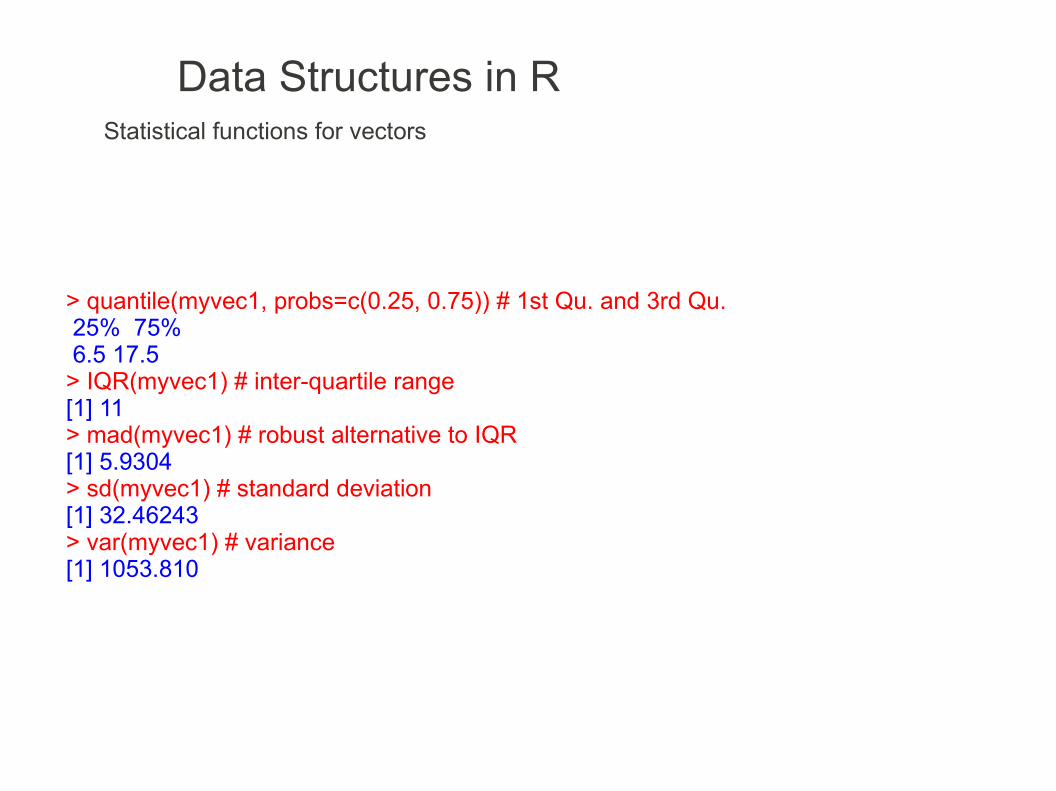
> quantile(myvec1, probs=c(0.25, 0.75)) # 1st Qu. and 3rd Qu. 25% 75% 6.5 17.5 > IQR(myvec1) # inter-quartile range[1] 11> mad(myvec1) # robust alternative to IQR[1] 5.9304> sd(myvec1) # standard deviation[1] 32.46243> var(myvec1) # variance[1] 1053.810
Statistical functions for vectors

Data Structures in R
any(..., na.rm = FALSE) returns TRUE if at least one value is TRUEall(..., na.rm = FALSE) returns TRUE if all the values are TRUE
na.rm = TRUE will ignore all the NAs
> #compare vectors, all elements are equal> x <- c(7, 5, 6)> y <- c(7, 5, 6)> x==y[1] TRUE TRUE TRUE> all(x==y)[1] TRUE> any(x==y)[1] TRUE> > #compare vectors, one element is equal> x <- c(7, 5, 6)> y <- c(7, 8, 9)> x==y[1] TRUE FALSE FALSE> all(x==y)[1] FALSE> any(x==y)[1] TRUE
> #compare vectors, regardless of element position> x <- c(7, 5, 6)> y <- c(5, 7, 6)> x==y[1] FALSE FALSE TRUE> sort(x)==sort(y)[1] TRUE TRUE TRUE

Data Structures in R
> # comparing 2 vectors, by position and with NAs> x <- y <- c(7, 6, NA, NA, 5)> all(x==y)[1] NA> all(x==y , na.rm = TRUE)[1] TRUE> identical(x, y)[1] TRUE> all.equal(x, y)[1] TRUE> x[!is.na(x)]==y[!is.na(y)][1] TRUE TRUE TRUE> all( x[!is.na(x)]==y[!is.na(y)] )[1] TRUE> > # NA OR TRUE is TRUE> # this will return TRUE despite the NAs> any(x==y)[1] TRUE> # this will return NA, not FALSE> y <- c(1, NA, 2, 3, 4)> any(x==y)[1] NA
Data Structures in RMatrix
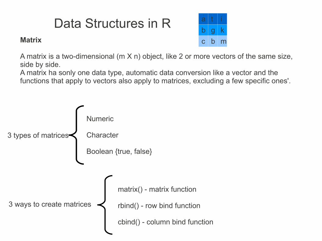
A matrix is a two-dimensional (m X n) object, like 2 or more vectors of the same size, side by side.A matrix ha sonly one data type, automatic data conversion like a vector and the functions that apply to vectors also apply to matrices, excluding a few specific ones'.
a t i
b g k
c b m
Numeric
Character
Boolean {true, false}
matrix() - matrix function
rbind() - row bind function
cbind() - column bind function
3 types of matrices
3 ways to create matrices
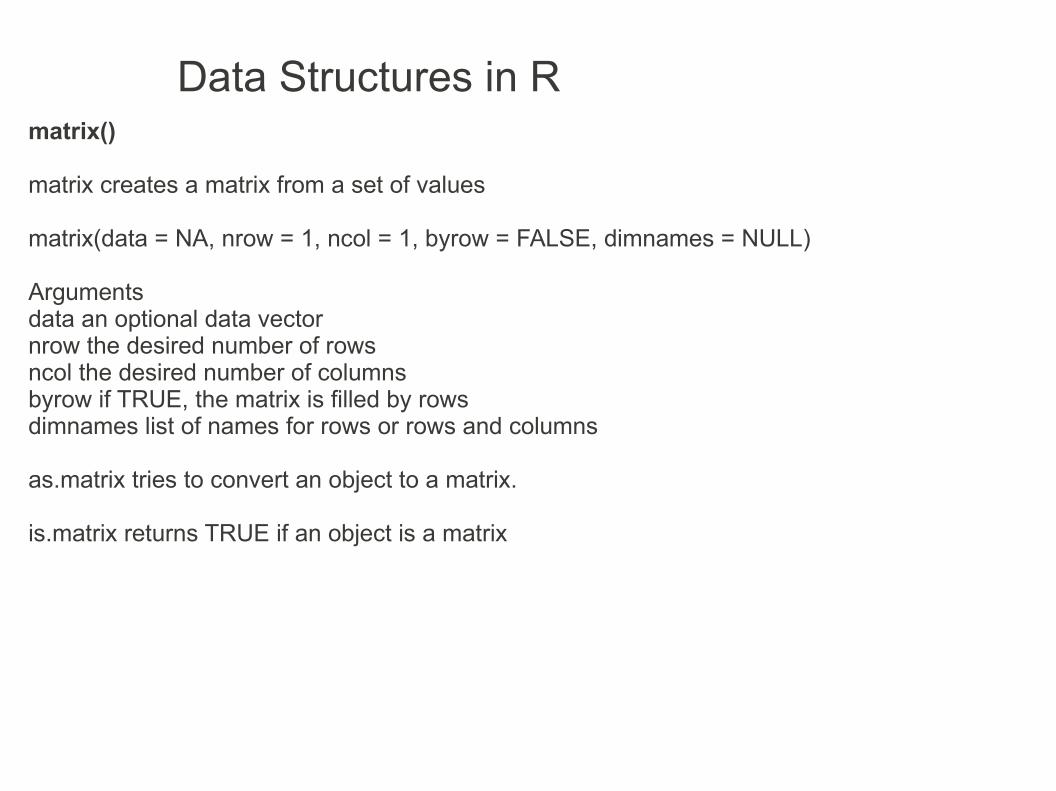
matrix()
matrix creates a matrix from a set of values
matrix(data = NA, nrow = 1, ncol = 1, byrow = FALSE, dimnames = NULL)
Argumentsdata an optional data vectornrow the desired number of rowsncol the desired number of columnsbyrow if TRUE, the matrix is filled by rowsdimnames list of names for rows or rows and columns
as.matrix tries to convert an object to a matrix.
is.matrix returns TRUE if an object is a matrix
Data Structures in R

Data Structures in R> matrix(10,3,2) # matrix 3 x 2 with 5's [,1] [,2][1,] 10 10[2,] 10 10[3,] 10 10> matrix(c(1,2,3),3,2)# matrix 3 x 2 with 2 columns with values [1,2,3] [,1] [,2][1,] 1 1[2,] 2 2[3,] 3 3> matrix(c(1,2),3,2,byrow = T)# matrix 3 x 2 with 3 rows with values [1,2] [,1] [,2][1,] 1 2[2,] 1 2[3,] 1 2> matrix(1:6,3,2)# matrix 3 x 2 with ascending values from each column [,1] [,2][1,] 1 4[2,] 2 5[3,] 3 6> matrix(1:6,3,2,byrow = T)# matrix 3 x 2 with ascending values from each row [,1] [,2][1,] 1 2[2,] 3 4[3,] 5 6

Data Structures in R
> mymatrix <- matrix(1:6,2,3,dimnames = list(c("row1", "row2"),c("col1", "col2", "col3")))> mymatrix # row and column names col1 col2 col3row1 1 3 5row2 2 4 6> mymatrix1 <- matrix(1:6,2,3,dimnames = list(c("row1", "row2")))> mymatrix1 # row names [,1] [,2] [,3]row1 1 3 5row2 2 4 6> mymatrix2 <- matrix(1:6,2,3,dimnames = list(NULL,c("col1", "col2", "col3")))> mymatrix2 # column names col1 col2 col3[1,] 1 3 5[2,] 2 4 6
Setting row and column names
Data Structures in R
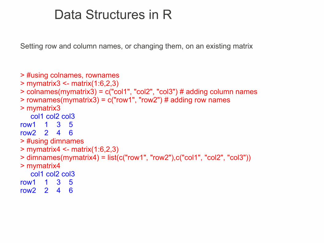
> #using colnames, rownames> mymatrix3 <- matrix(1:6,2,3)> colnames(mymatrix3) = c("col1", "col2", "col3") # adding column names> rownames(mymatrix3) = c("row1", "row2") # adding row names> mymatrix3 col1 col2 col3row1 1 3 5row2 2 4 6> #using dimnames> mymatrix4 <- matrix(1:6,2,3)> dimnames(mymatrix4) = list(c("row1", "row2"),c("col1", "col2", "col3"))> mymatrix4 col1 col2 col3row1 1 3 5row2 2 4 6
Setting row and column names, or changing them, on an existing matrix

Data Structures in R
cbind(), rbind()
Combine vector, matrix or data frames by columns or rows
> myvec <- seq(0,by=2, length.out= 8)> rbind(myvec, 1:8) [,1] [,2] [,3] [,4] [,5] [,6] [,7] [,8]myvec 0 2 4 6 8 10 12 14 1 2 3 4 5 6 7 8> cbind(myvec, 1:8) myvec [1,] 0 1[2,] 2 2[3,] 4 3[4,] 6 4[5,] 8 5[6,] 10 6[7,] 12 7[8,] 14 8
Data Structures in RExtracting matrix elements
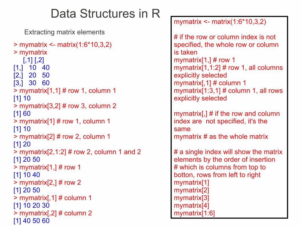
> mymatrix <- matrix(1:6*10,3,2)> mymatrix [,1] [,2][1,] 10 40[2,] 20 50[3,] 30 60> mymatrix[1,1] # row 1, column 1[1] 10> mymatrix[3,2] # row 3, column 2[1] 60> mymatrix[1] # row 1, column 1[1] 10> mymatrix[2] # row 2, column 1[1] 20> mymatrix[2,1:2] # row 2, column 1 and 2[1] 20 50> mymatrix[1,] # row 1[1] 10 40> mymatrix[2,] # row 2[1] 20 50> mymatrix[,1] # column 1[1] 10 20 30> mymatrix[,2] # column 2[1] 40 50 60
mymatrix <- matrix(1:6*10,3,2)
# if the row or column index is not specified, the whole row or column is takenmymatrix[1,] # row 1mymatrix[1,1:2] # row 1, all columns explicitly selectedmymatrix[,1] # column 1mymatrix[1:3,1] # column 1, all rows explicitly selected
mymatrix[,] # if the row and column index are not specified, it's the same mymatrix # as the whole matrix
# a single index will show the matrix elements by the order of insertion# which is columns from top to botton, rows from left to rightmymatrix[1]mymatrix[2]mymatrix[3]mymatrix[4]mymatrix[1:6]

Data Structures in R
> mymatrix <- matrix(1:6*10,3,2)> mymatrix [,1] [,2][1,] 10 40[2,] 20 50[3,] 30 60> mymatrix[-1,-1] # remove row 1 and column 1[1] 50 60> mymatrix[-1,] # remove row 1 [,1] [,2][1,] 20 50[2,] 30 60> mymatrix[-2,] # remove row 2 [,1] [,2][1,] 10 40[2,] 30 60> mymatrix[,-1] # remove column 1[1] 40 50 60> mymatrix[,-2] # remove column 2[1] 10 20 30
Negative indices remove rows or columns

Extracting matrix elements by row or column names
Data Structures in R
> mymatrix <- matrix(1:6*10,2,3,dimnames = list(c("row1", "row2"),c("col1", "col2", "col3")))> mymatrix col1 col2 col3row1 10 30 50row2 20 40 60> mymatrix["row1","col1"]# row 1, column 1[1] 10> mymatrix["row2",]# row 2col1 col2 col3 20 40 60 > mymatrix[,c("col1","col3")]# column 1 and column 3 col1 col3row1 10 50row2 20 60

> mymatrix <- matrix(1:6*10,2,3,dimnames = list(c("row1", "row2"),c("col1", "col2", "col3")))> mymatrix col1 col2 col3row1 10 30 50row2 20 40 60> dim(mymatrix) # dimensions of the matrix, 2 x 3[1] 2 3> length(mymatrix) # number of elements[1] 6> dimnames(mymatrix) # dimension names (rows and columns names')[[1]][1] "row1" "row2"
[[2]][1] "col1" "col2" "col3"
> colnames(mymatrix) # rows names[1] "col1" "col2" "col3"> rownames(mymatrix) # columns names[1] "row1" "row2"> mode(mymatrix) # Storage Mode of this Object[1] "numeric"> is(mymatrix) # all the super-classes of this object's class[1] "matrix" "array" "structure" "vector" > class(mymatrix) # class attribute or the implicit class of this object[1] "matrix"
Data Structures in RMatrix info
Data Structures in R
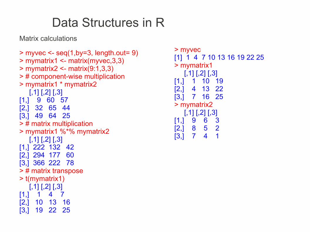
> myvec <- seq(1,by=3, length.out= 9)> mymatrix1 <- matrix(myvec,3,3)> mymatrix2 <- matrix(9:1,3,3)> # component-wise multiplication> mymatrix1 * mymatrix2 [,1] [,2] [,3][1,] 9 60 57[2,] 32 65 44[3,] 49 64 25> # matrix multiplication> mymatrix1 %*% mymatrix2 [,1] [,2] [,3][1,] 222 132 42[2,] 294 177 60[3,] 366 222 78> # matrix transpose> t(mymatrix1) [,1] [,2] [,3][1,] 1 4 7[2,] 10 13 16[3,] 19 22 25
> myvec [1] 1 4 7 10 13 16 19 22 25> mymatrix1 [,1] [,2] [,3][1,] 1 10 19[2,] 4 13 22[3,] 7 16 25> mymatrix2 [,1] [,2] [,3][1,] 9 6 3[2,] 8 5 2[3,] 7 4 1
Matrix calculations
Data Structures in RMatrix calculations
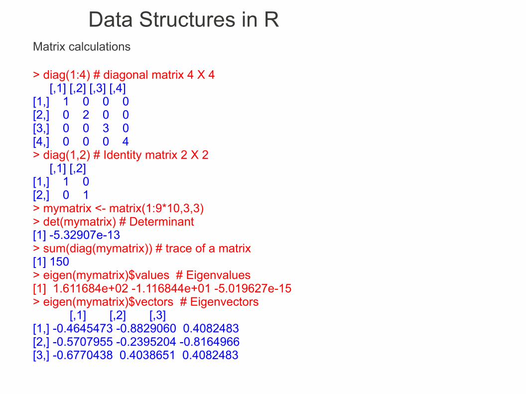
> diag(1:4) # diagonal matrix 4 X 4 [,1] [,2] [,3] [,4][1,] 1 0 0 0[2,] 0 2 0 0[3,] 0 0 3 0[4,] 0 0 0 4> diag(1,2) # Identity matrix 2 X 2 [,1] [,2][1,] 1 0[2,] 0 1> mymatrix <- matrix(1:9*10,3,3)> det(mymatrix) # Determinant[1] -5.32907e-13> sum(diag(mymatrix)) # trace of a matrix[1] 150> eigen(mymatrix)$values # Eigenvalues[1] 1.611684e+02 -1.116844e+01 -5.019627e-15> eigen(mymatrix)$vectors # Eigenvectors [,1] [,2] [,3][1,] -0.4645473 -0.8829060 0.4082483[2,] -0.5707955 -0.2395204 -0.8164966[3,] -0.6770438 0.4038651 0.4082483

Data Structures in RMatrix calculations
chol() Choleski factorization of a real symmetric positive-definite square matrixqr() QR decomposition of a matrixsvd() singular-value decomposition of a rectangular matrixcrossprod() matrix cross-productouter() outer product of arrays scale() Scaling and centering of matrixsolve() Solve a system of equationssvd() singular-value decomposition of a rectangular matrix
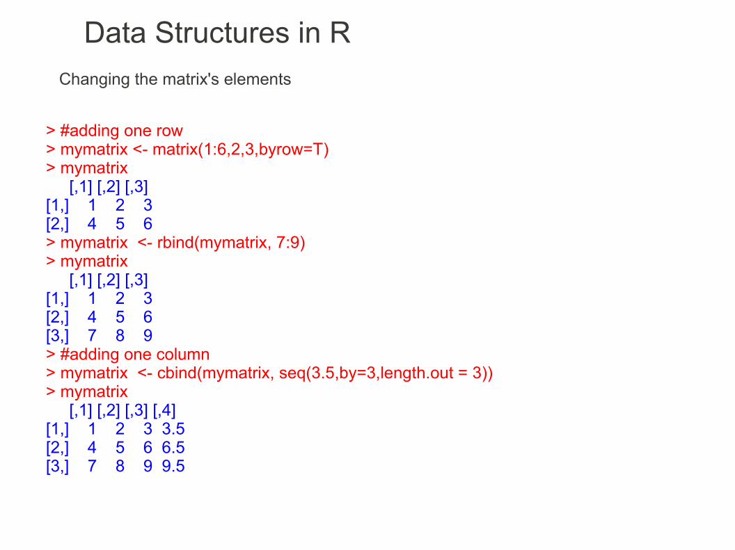
Changing the matrix's elements
Data Structures in R
> #adding one row> mymatrix <- matrix(1:6,2,3,byrow=T)> mymatrix [,1] [,2] [,3][1,] 1 2 3[2,] 4 5 6> mymatrix <- rbind(mymatrix, 7:9)> mymatrix [,1] [,2] [,3][1,] 1 2 3[2,] 4 5 6[3,] 7 8 9> #adding one column> mymatrix <- cbind(mymatrix, seq(3.5,by=3,length.out = 3))> mymatrix [,1] [,2] [,3] [,4][1,] 1 2 3 3.5[2,] 4 5 6 6.5[3,] 7 8 9 9.5
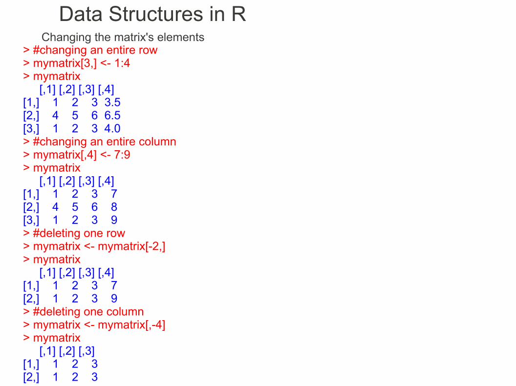
Changing the matrix's elements
Data Structures in R
> #changing an entire row> mymatrix[3,] <- 1:4> mymatrix [,1] [,2] [,3] [,4][1,] 1 2 3 3.5[2,] 4 5 6 6.5[3,] 1 2 3 4.0> #changing an entire column> mymatrix[,4] <- 7:9> mymatrix [,1] [,2] [,3] [,4][1,] 1 2 3 7[2,] 4 5 6 8[3,] 1 2 3 9> #deleting one row> mymatrix <- mymatrix[-2,]> mymatrix [,1] [,2] [,3] [,4][1,] 1 2 3 7[2,] 1 2 3 9> #deleting one column> mymatrix <- mymatrix[,-4]> mymatrix [,1] [,2] [,3][1,] 1 2 3[2,] 1 2 3

Data Structures in RApplying functions on matrix/array elements
apply() returns a vector or array or list, after applying a function to each of its members
apply(object, margin, function, ...)
object is the input arraymargin are the subscripts where to apply the function, 1 indicates rows, 2 indicates columns, c(1,2) indicates rows and columnsfunction ... optional arguments for the function
> mymatrix <- matrix(1:6*10,2,3)> mymatrix [,1] [,2] [,3][1,] 10 30 50[2,] 20 40 60> apply(mymatrix,1,max) # rows[1] 50 60> apply(mymatrix,2,max) # columns[1] 20 40 60> apply(mymatrix,c(1,2),max) # rows and columns, useless
#try:apply(mymatrix,1,mean) # rowsapply(mymatrix,2,mean) # columns
#try:apply(mymatrix,1,sort) # rowsapply(mymatrix,2,sort) # columns

Data Structures in R
Array
An array is a three-dimensional (m X n X p) object, like 2 or more matrices of the same dimensions, side by side.An array has only one data type, automatic data conversion like a vector or matrix and the functions that apply to vectors and matrices also apply to arraya, excluding a few specific ones'.
array(data = NA, dim = length(data), dimnames = NULL) creates an array from data, dim are the dimensions and dimnames are optional names for the dimensions
as.array() tries to convert an object to an array
is.array() returns TRUE if the object is an array
2 6 10 14
8 19 17 16
1 5 9 13
3 7 11 15
=
Dimension z = 1
Dimension z = 2

Data Structures in R2 6 10 14
8 19 17 16
1 5 9 13
3 7 11 15
=
> array(c(1,3,5,7,9,11,13,15,2,8,6,19,10,17,14,16),c(2,4,2)), , 1
[,1] [,2] [,3] [,4][1,] 1 5 9 13[2,] 3 7 11 15
, , 2
[,1] [,2] [,3] [,4][1,] 2 6 10 14[2,] 8 19 17 16
Notice how the element values are inserted by column

Data Structures in R2 6 10 14
8 19 17 16
1 5 9 13
3 7 11 15
=
> # turning matrices into arrays> # passing data by rows> m1 <- matrix(c(1,5,9,13,3,7,11,15),2,4, byrow=T)> m2 <- matrix(c(2,6,10,14,8,19,17,16),2,4, byrow=T)> array(c(m1,m2),c(2,4,2)), , 1
[,1] [,2] [,3] [,4][1,] 1 5 9 13[2,] 3 7 11 15
, , 2
[,1] [,2] [,3] [,4][1,] 2 6 10 14[2,] 8 19 17 16

Data Structures in R
Adding dimension names
56 174 75 77
67 166 55 70Men
Women
CityAge Hgt Wgt BPM
64 178 78 63
77 170 59 61Men
Women
CountrysideAge Hgt Wgt BPM
This data is fake, can anyone get real data?
> myarray<-array(c(56,67,174,166,75,55,77,70,64,77,178,170,78,59,63,61),c(2,4,2))> dimnames(myarray) = list(c("men","women"),c("age","height","weight","pulse"),+ c("city","countryside"))> myarray, , city
age height weight pulsemen 56 174 75 77women 67 166 55 70
, , countryside
age height weight pulsemen 64 178 78 63women 77 170 59 61
# dimension names defined directly:myarray2<-array(c(56,67,174,166,75,55,77,70,64,77,178,170,78,59,63,61),c(2,4,2), dimnames = list(c("men","women"),c("age","height","weight","pulse"),c("city","countryside")))
or

Data Structures in RAccesing the array's elements
City
Age Hgt Wgt BPM
64 178 78 63
77 170 59 6156 174 75 77
67 166 55 70
MenWomen
CountrysideAge Hgt Wgt BPM
MenWomen
> dimnames(myarray)[[1]][1] "men" "women"
[[2]][1] "age" "height" "weight" "pulse"
[[3]][1] "city" "countryside"
> myarray["women",,] # women's all info, all cities city countrysideage 67 77height 166 170weight 55 59pulse 70 61> myarray["women",,"countryside"] # women's all info, countryside age height weight pulse 77 170 59 61 > myarray[,,"countryside"] # all info, countryside age height weight pulsemen 64 178 78 63women 77 170 59 61> myarray[, "height",] # height city countrysidemen 174 178women 166 170
Same, with indices
myarray[2,,] # women's all info, all citiesmyarray[2,, 2] # women's all info, countrysidemyarray[,,2] # all info, countrysidemyarray[, 2,] # height

Data Structures in R
Operations on the array's elements
City
Age Hgt Wgt BPM
64 178 78 63
77 170 59 6156 174 75 77
67 166 55 70
MenWomen
CountrysideAge Hgt Wgt BPM
MenWomen
> apply(myarray,1,max) # rows men women 178 170 > apply(myarray,2,max) # columns age height weight pulse 77 178 78 77 > apply(myarray,c(1,2),max) # rows and columns age height weight pulsemen 64 178 78 77women 77 170 59 70
Meaningless, age vs htg...
Oldest, tallest...
Oldest, tallest... by gender
apply(myarray,2,mean) # columns mean apply(myarray,c(1,2),mean) # rows and columns mean apply(myarray,2,quantile) # columns quartilesapply(myarray,c(1,2),quantile) # rows and columns quartiles
apply(myarray,2,quantile,.5) # columns median

Changing the array's elements
Data Structures in R
City
Age Hgt Wgt BPM
64 178 78 63
77 170 59 6156 174 75 77
67 166 55 70
MenWomen
CountrysideAge Hgt Wgt BPM
MenWomen
myarray <- array(c(56,67,174,166,75,55,77,70,64,77,178,170,78,59,63,61),c(2,4,2))dimnames(myarray) = list(c("men","women"),c("age","height","weight","pulse"), c("city","countryside"))
myarray <- myarray[, -4,] # remove pulse, by indexmyarray <- myarray[, colnames(myarray) != "age",] # remove age, by column name
myarray <- array(c(myarray,c(167,162,75,60,179,168,77,65)),c(2,2,4)) # adding 2 "places"dimnames(myarray) = list(c("men","women"),c("height","weight"), c("city","countryside", "p1","p2"))

Data Structures in RList
A list is a vector containing elements of different types
The elements are accessible by indices, like on a vector, there is just an extra square bracket [ ] for the list index and there might be other indices from contained elements.
vectormatrixarraydataframelist
> myvec <- 3:8> mymatrix <- matrix(6:1*10,3,2)> mydataframe <- as.data.frame(mymatrix)> mylist <- list(myvec, mymatrix, mydataframe, 56,"test")> mylist[[1]][1][1] 3> mylist[[1]][2][1] 4> mylist[[2]][1,1][1] 60> mylist[[3]]$V1[2][1] 50> mylist[[4]][1] 56> mylist[[5]][1] "test"
> mylist[[1]][1] 3 4 5 6 7 8
[[2]] [,1] [,2][1,] 60 30[2,] 50 20[3,] 40 10
[[3]] V1 V21 60 302 50 203 40 10
[[4]][1] 56
[[5]][1] "test"
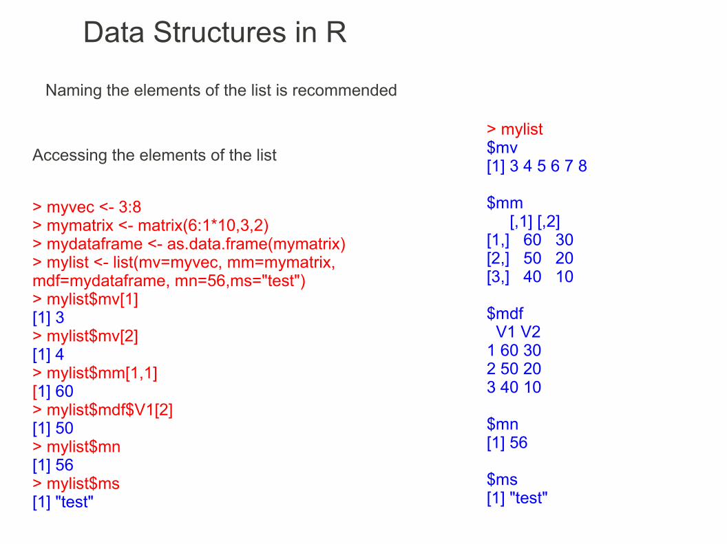
Data Structures in R
> myvec <- 3:8> mymatrix <- matrix(6:1*10,3,2)> mydataframe <- as.data.frame(mymatrix)> mylist <- list(mv=myvec, mm=mymatrix, mdf=mydataframe, mn=56,ms="test")> mylist$mv[1][1] 3> mylist$mv[2][1] 4> mylist$mm[1,1][1] 60> mylist$mdf$V1[2][1] 50> mylist$mn[1] 56> mylist$ms[1] "test"
Naming the elements of the list is recommended
> mylist$mv[1] 3 4 5 6 7 8
$mm [,1] [,2][1,] 60 30[2,] 50 20[3,] 40 10
$mdf V1 V21 60 302 50 203 40 10
$mn[1] 56
$ms[1] "test"
Accessing the elements of the list

Data Structures in R
myvec <- 3:8mymatrix <- matrix(6:1*10,3,2)mydataframe <- as.data.frame(mymatrix)mylist <- list(myvec, mymatrix, mydataframe, 56,"test")is(mylist) # list, of courselength(mylist)dim(mylist) # the dimensions of the elements don't countmylist[1] # [1] <=> [[1]]mylist[2]mylist[3]mylist[4]mylist[5]is(mylist[1]) # each element is a listis(mylist[2])is(mylist[3])is(mylist[4])is(mylist[5])mylist[1:3]

Data Structures in R
Changing the elements of the list
> mylist$mv[1] 3 4 5 6 7 8
$mm [,1] [,2][1,] 60 30[2,] 50 20[3,] 40 10
$mdf V1 V21 60 302 50 203 40 10
$mn[1] 56
$ms[1] "test"
myvec <- 3:8mymatrix <- matrix(6:1*10,3,2)mydataframe <- as.data.frame(mymatrix)mylist <- list(mv=myvec, mm=mymatrix, mdf=mydataframe, mn=56,ms="test")# updating one elementmylist$ms <- "new test"mylist$msmylist[[5]] <- "newer test"mylist$ms# inserting two elementsmylist <- c(mylist,wname="Friday", mday=13)mylist# deleting one element at a timemylist$ms<- NULLmylist[["mn"]]<- NULLmylist[[1]]<- NULLmylist

Data Structures in R
Using the $ notation
myvec <- 3:8mymatrix <- matrix(6:1*10,3,2)mydataframe <- as.data.frame(mymatrix)mylist <- list(mv=myvec, mm=mymatrix, mdf=mydataframe, mn=56,ms="test")# inserting one elementmylist <- c(mylist,tree_info=list(family="Fagaceae", genus ="Fagus"))mylistmylist$tree_info # this is NULL, must specify the sub-elementsmylist$tree_info.familymylist$tree_info.genusmylist[["tree_info.family"]]

Data Structures in RFactors
A factor is a vector that specifies a discrete clasification of other vectors. Factors store categorical data, qualitative values, non numeric such as gender, job, color, species, model, brand, etc... Or numeric but meaningless like model numbers or site numbers or zip codes.> student.residence <- c("Helsinki","Tampere","Turku","Helsinki","Helsinki","Turku","Oulu","Tampere","Helsinki","Turku","Tampere","Helsinki")> student.residence [1] "Helsinki" "Tampere" "Turku" "Helsinki" "Helsinki" "Turku" [7] "Oulu" "Tampere" "Helsinki" "Turku" "Tampere" "Helsinki"> fstudent=as.factor(student.residence)> fstudent [1] Helsinki Tampere Turku Helsinki Helsinki Turku Oulu Tampere [9] Helsinki Turku Tampere HelsinkiLevels: Helsinki Oulu Tampere Turku> levels(fstudent)[1] "Helsinki" "Oulu" "Tampere" "Turku" > summary(fstudent)Helsinki Oulu Tampere Turku 5 1 3 3 > student.height=c(175,162,170,170,192,170,115,155,150,130,220,160)> student.height [1] 175 162 170 170 192 170 115 155 150 130 220 160> tapply(student.height,fstudent,mean)Helsinki Oulu Tampere Turku 169.4000 115.0000 179.0000 156.6667

Sorted factors
Factor with levels of hierarchy
function ordered() turns a factor into a sorted factor
Data Structures in R
> # sort the cities by increasing longitude> flevel.residence <- ordered(student.residence, levels=c("Helsinki","Turku","Tampere","Oulu"))> flevel.residence [1] Helsinki Tampere Turku Helsinki Helsinki Turku Oulu Tampere [9] Helsinki Turku Tampere HelsinkiLevels: Helsinki < Turku < Tampere < Oulu> # check each student whether he/she lives south of Tampere> flevel.residence < "Tampere" [1] TRUE FALSE TRUE TRUE TRUE TRUE FALSE FALSE TRUE TRUE FALSE TRUE
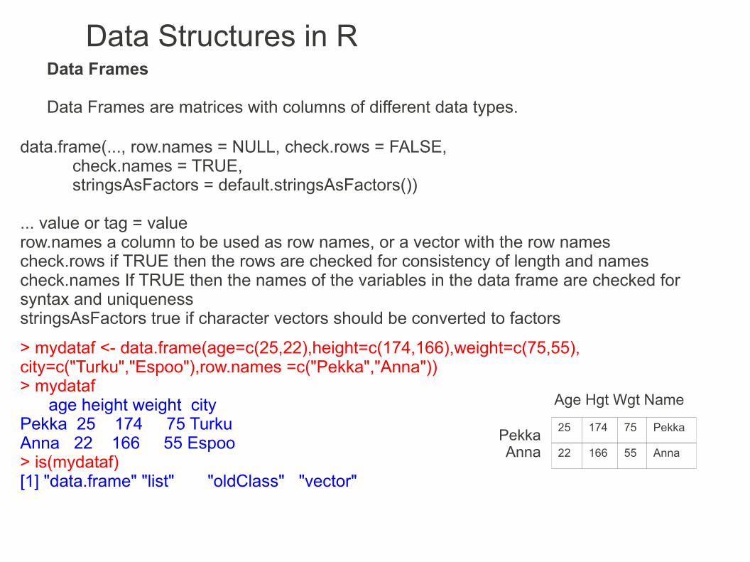
Data Structures in RData Frames
Data Frames are matrices with columns of different data types.
data.frame(..., row.names = NULL, check.rows = FALSE, check.names = TRUE, stringsAsFactors = default.stringsAsFactors())
... value or tag = valuerow.names a column to be used as row names, or a vector with the row names check.rows if TRUE then the rows are checked for consistency of length and namescheck.names If TRUE then the names of the variables in the data frame are checked for syntax and uniquenessstringsAsFactors true if character vectors should be converted to factors
25 174 75 Pekka
22 166 55 Anna
PekkaAnna
Age Hgt Wgt Name
> mydataf <- data.frame(age=c(25,22),height=c(174,166),weight=c(75,55), city=c("Turku","Espoo"),row.names =c("Pekka","Anna"))> mydataf age height weight cityPekka 25 174 75 TurkuAnna 22 166 55 Espoo> is(mydataf)[1] "data.frame" "list" "oldClass" "vector"

Data Structures in RAccessing the data frame's elements
> #getting the info for Anna> mydataf[2,] # by index, row 2 age height weight cityAnna 22 166 55 Espoo> mydataf["Anna",] # by key age height weight cityAnna 22 166 55 Espoo> #getting the weight for everybody> mydataf[,3] # by index, column 3[1] 75 55> mydataf[,"weight"] # by key[1] 75 55> mydataf$weight # by list key[1] 75 55

Data Structures in RSorting the data frame's elements
mydataf <- data.frame(age=c(25,22,26,28),height=c(174,166,174,170),weight=c(75,55,60,60), city=c("Turku","Espoo","Kuopio","Helsinki"),row.names =c("Pekka","Anna","Ari","Tove"))mydataf
#order by heightorder(mydataf$height)#order by nameorder(row.names(mydataf))#order by height and weightorder(mydataf$height, mydataf$weight)
#order by heightmydataf[order(mydataf$height),]#order by namemydataf[order(row.names(mydataf)),]#order by height and weightmydataf[order(mydataf$height, mydataf$weight),]#order by height and weight, both decreasingmydataf[order(mydataf$height, mydataf$weight, decreasing = T),]#order by decreasing height and increasing weightmydataf[order(-mydataf$height, mydataf$weight),]

Changing the data frame's elementsData Structures in R
> mydataf <- data.frame(age=c(25,22),height=c(174,166),weight=c(75,55), city=c("Turku","Espoo"),row.names =c("Pekka","Anna"))> mydataf age height weight cityPekka 25 174 75 TurkuAnna 22 166 55 Espoo> mydataf <- cbind(mydataf,course=c("Math","Art")) # adding a column> mydataf age height weight city coursePekka 25 174 75 Turku MathAnna 22 166 55 Espoo Art> mydataf <- data.frame(mydataf, hobby=c("walking","reading")) # adding a column> mydataf age height weight city course hobbyPekka 25 174 75 Turku Math walkingAnna 22 166 55 Espoo Art reading> mydataf <- rbind(mydataf, zed=data.frame(age=28,height=199,weight=115,city="Oulu",course="Sports",hobby="sleep")) # adding a row> mydataf age height weight city course hobbyPekka 25 174 75 Turku Math walkingAnna 22 166 55 Espoo Art readingzed 28 199 115 Oulu Sports sleep

Data Structures in ROperations on the data frame's elements
> mean(mydataf[,1]) # the mean of all ages[1] 23.5> mean(mydataf[,c("height","weight")]) # the mean of height, weight height weight 170 65 > apply(mydataf,2,mean) # ERROR! age height weight city NA NA NA NA Warning messages:1: In mean.default(newX[, i], ...) : argument is not numeric or logical: returning NA2: In mean.default(newX[, i], ...) : argument is not numeric or logical: returning NA3: In mean.default(newX[, i], ...) : argument is not numeric or logical: returning NA4: In mean.default(newX[, i], ...) : argument is not numeric or logical: returning NA> apply(mydataf[,1:3],2,mean) # the mean of age, height, weight age height weight 23.5 170.0 65.0
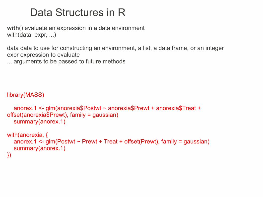
Data Structures in Rwith() evaluate an expression in a data environmentwith(data, expr, ...)
data data to use for constructing an environment, a list, a data frame, or an integerexpr expression to evaluate... arguments to be passed to future methods
library(MASS) anorex.1 <- glm(anorexia$Postwt ~ anorexia$Prewt + anorexia$Treat + offset(anorexia$Prewt), family = gaussian) summary(anorex.1)
with(anorexia, { anorex.1 <- glm(Postwt ~ Prewt + Treat + offset(Prewt), family = gaussian) summary(anorex.1)})

Data Structures in Rlapply, sapply applies a function over a list or vector
lapply returns a list of the same length as X, each element of which is the result of applying FUN to the corresponding element of X
sapply is a user-friendly version of lapply by default returning a vector or matrix if appropriate
lapply(X, FUN, ...)
sapply(X, FUN, ..., simplify = TRUE, USE.NAMES = TRUE)
X a vector (atomic or list) or an expressions vectorFUN the function to be applied to each element of X... optional arguments to FUNsimplify if TRUE the result is simplified to a vector or matrix if possibleUSE.NAMES if TRUE and if X is character, use X as names for the result unless it had names alreadyn number of replicationsexpr expression to evaluate repeatedly
at1 <- list(athlete="Johnson",coach="Earp",swimming=c(154,171,165), cycling=c(598,632,621), running=c(1046,1102,1095),wetsuit=c(T,F,T))# compute the list mean for each list elementmean(at1)mean(at1$swimming) # one at at time...lapply(at1,mean)sapply(at1,mean)

Statistical functions
mydataf <- data.frame(age=c(25,22),height=c(174,166),weight=c(75,55),city=c("Turku","Espoo"),row.names =c("Pekka","Anna"))mydatafsapply(mydataf, mean, na.rm=TRUE)
Other functions useful for sapply:
sd, var, min, max, med, range, and quantile
summary will return the Min. 1st Qu. Median Mean 3rd Qu. Max.
summary(mydataf)
fivenum will return Tukey's five number summary (minimum, lower-hinge, median, upper-hinge, maximum)
fivenum(mydataf[1:3])
Data Structures in R

# Concatenate stringspaste("a","b","c")paste("a","b","c",sep="")
# Concatenate a vector of stringsmyvec <- c("a","b","c")paste(myvec)paste(myvec,sep="",collapse="")
# extract part of the stringmystr <- "Hello world!"substring(mystr, 7, 11)
# split a string into each charactermystr <- "Hello world!"strsplit(mystr, "")
# split a string into pieces, using regexmystr <- "Hello world!"strsplit(mystr, " ")strsplit(mystr, "\\s")strsplit(mystr, "[\\seo]")
string functions
Data Structures in R
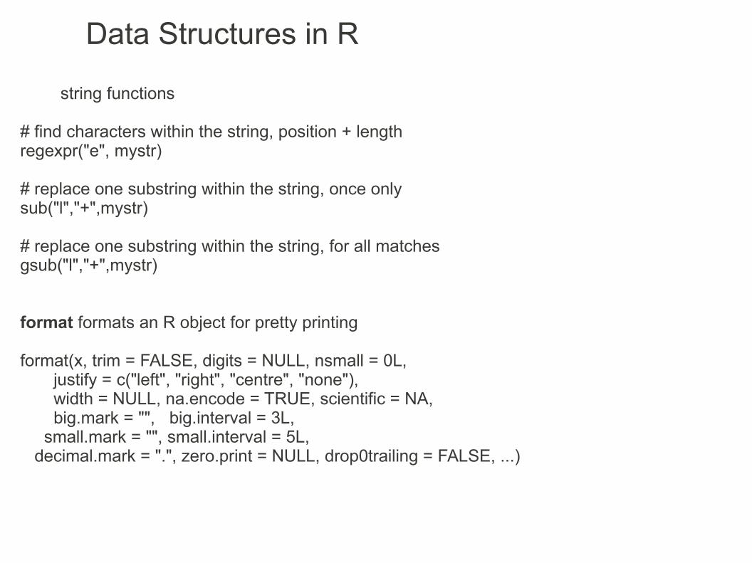
# find characters within the string, position + lengthregexpr("e", mystr)
# replace one substring within the string, once onlysub("l","+",mystr)
# replace one substring within the string, for all matchesgsub("l","+",mystr)
format formats an R object for pretty printing
format(x, trim = FALSE, digits = NULL, nsmall = 0L, justify = c("left", "right", "centre", "none"), width = NULL, na.encode = TRUE, scientific = NA, big.mark = "", big.interval = 3L, small.mark = "", small.interval = 5L, decimal.mark = ".", zero.print = NULL, drop0trailing = FALSE, ...)
string functions
Data Structures in R
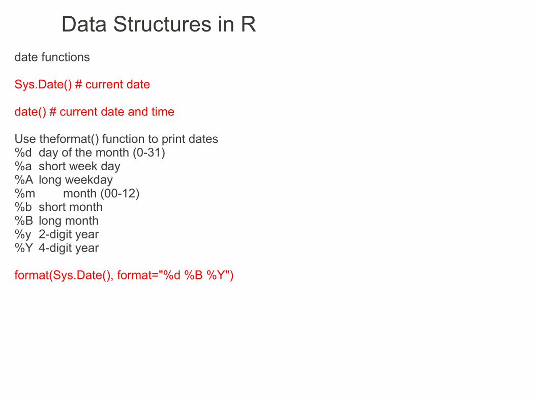
date functions
Sys.Date() # current date
date() # current date and time
Use theformat() function to print dates%d day of the month (0-31)%a short week day%A long weekday%m month (00-12)%b short month%B long month%y 2-digit year%Y 4-digit year
format(Sys.Date(), format="%d %B %Y")
Data Structures in R

Data Type Conversion
Checking the data type
is.numeric(), is.character(), is.vector(), is.matrix(), is.data.frame()
Explicit conversion
as.numeric(), as.character(), as.vector(), as.matrix(), as.data.frame)
Data Structures in R
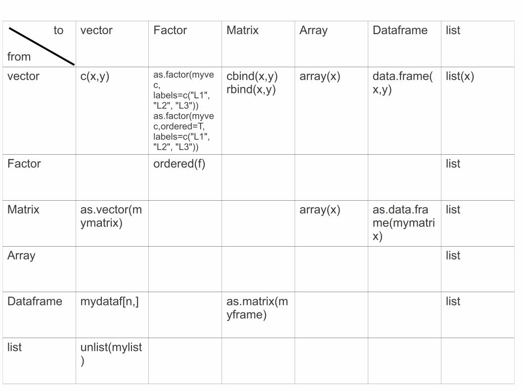
to
from
vector Factor Matrix Array Dataframe list
vector c(x,y) as.factor(myvec, labels=c("L1", "L2", "L3"))as.factor(myvec,ordered=T, labels=c("L1", "L2", "L3"))
cbind(x,y)rbind(x,y)
array(x) data.frame(x,y)
list(x)
Factor ordered(f) list
Matrix as.vector(mymatrix)
array(x) as.data.frame(mymatrix)
list
Array list
Dataframe mydataf[n,] as.matrix(myframe)
list
list unlist(mylist)

Data Structures in R
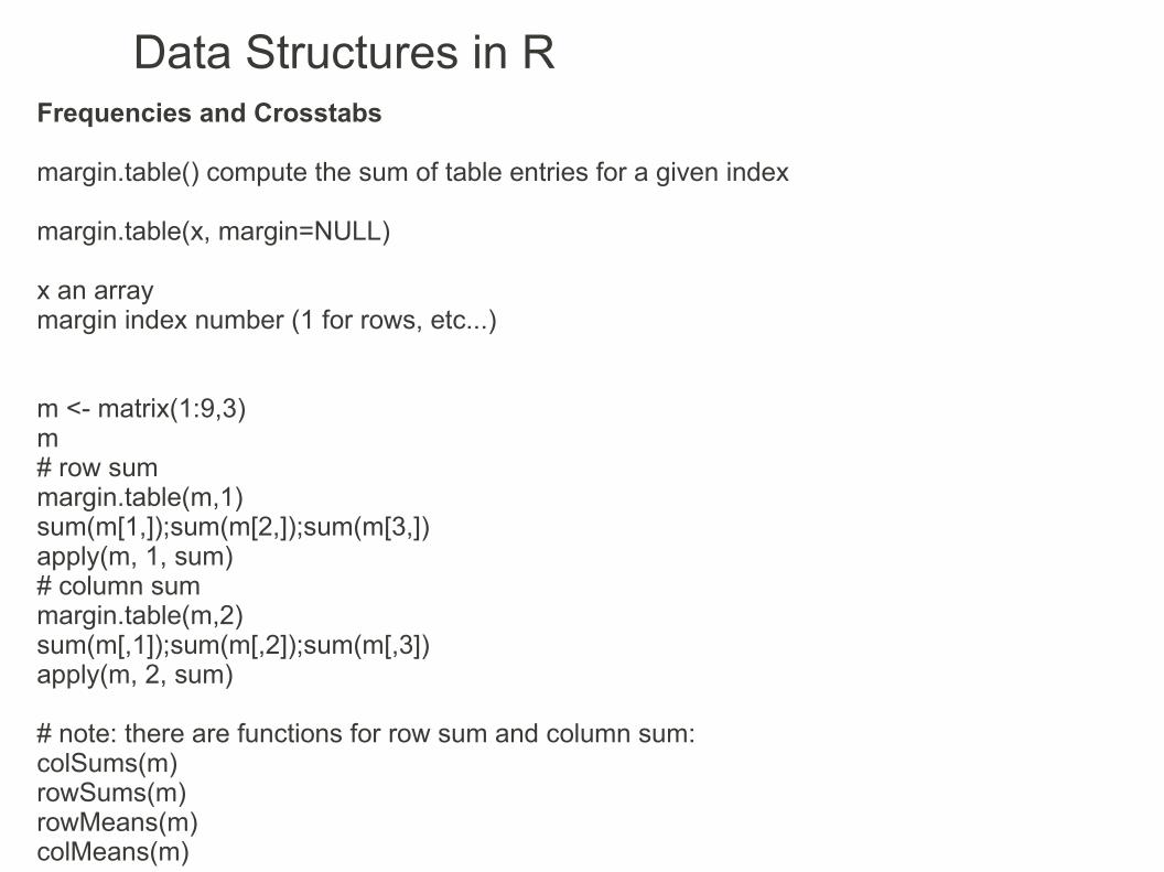
Data Structures in RFrequencies and Crosstabs
margin.table() compute the sum of table entries for a given index
margin.table(x, margin=NULL)
x an arraymargin index number (1 for rows, etc...)
m <- matrix(1:9,3)m# row summargin.table(m,1)sum(m[1,]);sum(m[2,]);sum(m[3,])apply(m, 1, sum)# column summargin.table(m,2)sum(m[,1]);sum(m[,2]);sum(m[,3])apply(m, 2, sum)
# note: there are functions for row sum and column sum:colSums(m)rowSums(m)rowMeans(m)colMeans(m)

Data Structures in RFrequencies and Crosstabs
prop.table() Express table entries as a fraction of the marginal table
prop.table(x, margin=NULL)
x tablemargin index, or vector of indices
m <- matrix(1:9,3)mprop.table(m) # cell percentagesprop.table(m, 1) # row percentagesprop.table(m, 2) # column percentages
prop.table(m) # cell percentagesm / sum(m)sweep(m,1, margin.table(m),"/")
prop.table(m, 1) # row percentagesm[1,]/sum(m[1,])m[2,]/sum(m[2,])m[3,]/sum(m[3,])sweep(m,1, margin.table(m,1),"/")
prop.table(m, 2) # column percentagesm[,1]/sum(m[,1])m[,2]/sum(m[,2])m[,3]/sum(m[,3])sweep(m,2, margin.table(m,2),"/")
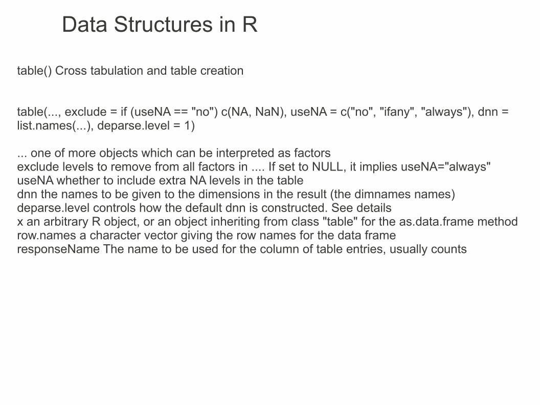
Data Structures in R
table() Cross tabulation and table creation
table(..., exclude = if (useNA == "no") c(NA, NaN), useNA = c("no", "ifany", "always"), dnn = list.names(...), deparse.level = 1)
... one of more objects which can be interpreted as factorsexclude levels to remove from all factors in .... If set to NULL, it implies useNA="always"useNA whether to include extra NA levels in the tablednn the names to be given to the dimensions in the result (the dimnames names)deparse.level controls how the default dnn is constructed. See detailsx an arbitrary R object, or an object inheriting from class "table" for the as.data.frame methodrow.names a character vector giving the row names for the data frameresponseName The name to be used for the column of table entries, usually counts

Data Structures in R
x <- sample(c("heads","tails"),5, replace=T)xfx <- factor(x)fxtable(fx)
mtcars?mtcarsis(mtcars)names(mtcars)dim(mtcars)rownames(mtcars);colnames(mtcars)dimnames(mtcars)# how many cars for each Number of cylinderstable(mtcars$cyl,dnn = list("Number of forward cylinders")) # how many cars for each Number of cylinders / Number of forward gearstable(mtcars$cyl,mtcars$gear,dnn = list("Number of cylinders","Number of forward gears")) # how many cars for each Number of cylinders / Number of forward gears / Transmissiontable(mtcars$cyl,mtcars$gear,mtcars$am,dnn = list("Number of cylinders","Number of forward gears","Transmission"))

xtabs() reate a contingency table from cross-classifying factors
xtabs(formula = ~., data = parent.frame(), subset, na.action, exclude = c(NA, NaN), drop.unused.levels = FALSE)
formula a formula object with the cross-classifying variables (separated by +) on the right hand sidedata an optional matrix or data frame containing the variables in the formula formulasubset an optional vector specifying a subset of observations to be usedna.action a function which indicates what should happen when the data contain NAsexclude a vector of values to be excluded when forming the set of levels of the classifying factorsdrop.unused.levels a logical indicating whether to drop unused levels in the classifying factors
# convert from table to dataframehair.df=as.data.frame(HairEyeColor)# convert from dataframe to tablextabs(Freq~Hair+Eye+Sex,data=hair.df)
# crosstabulation of Hair and Eyextabs(Freq~Hair+Eye,data=hair.df)# crosstabulation of Hair and Sexxtabs(Freq~Hair+Sex,data=hair.df)# crosstabulation of Eye and Sexxtabs(Freq~Eye+Sex,data=hair.df)
Data Structures in R
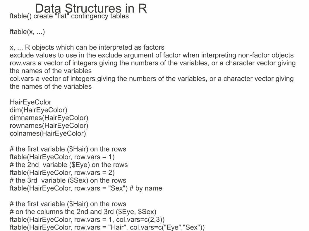
Data Structures in Rftable() create "flat" contingency tables
ftable(x, ...)
x, ... R objects which can be interpreted as factorsexclude values to use in the exclude argument of factor when interpreting non-factor objectsrow.vars a vector of integers giving the numbers of the variables, or a character vector giving the names of the variablescol.vars a vector of integers giving the numbers of the variables, or a character vector giving the names of the variables
HairEyeColordim(HairEyeColor)dimnames(HairEyeColor)rownames(HairEyeColor)colnames(HairEyeColor)
# the first variable ($Hair) on the rowsftable(HairEyeColor, row.vars = 1)# the 2nd variable ($Eye) on the rowsftable(HairEyeColor, row.vars = 2)# the 3rd variable ($Sex) on the rowsftable(HairEyeColor, row.vars = "Sex") # by name
# the first variable ($Hair) on the rows# on the columns the 2nd and 3rd ($Eye, $Sex)ftable(HairEyeColor, row.vars = 1, col.vars=c(2,3))ftable(HairEyeColor, row.vars = "Hair", col.vars=c("Eye","Sex"))

Data Structures in R
# the first variable ($Hair) on the rows# on the columns the 3rd and 2nd ($Sex,$Eye )ftable(HairEyeColor, row.vars = 1, col.vars=c(3,2))ftable(HairEyeColor, row.vars = "Hair", col.vars=c("Sex","Eye"))
# the first and 2nd variables ($Hair,$Eye) on the rowsftable(HairEyeColor, row.vars = 1:2)
# the first, 2nd and 3rd variables ($Hair,$Eye,$Sex) on the rowsftable(HairEyeColor, row.vars = 1:3)
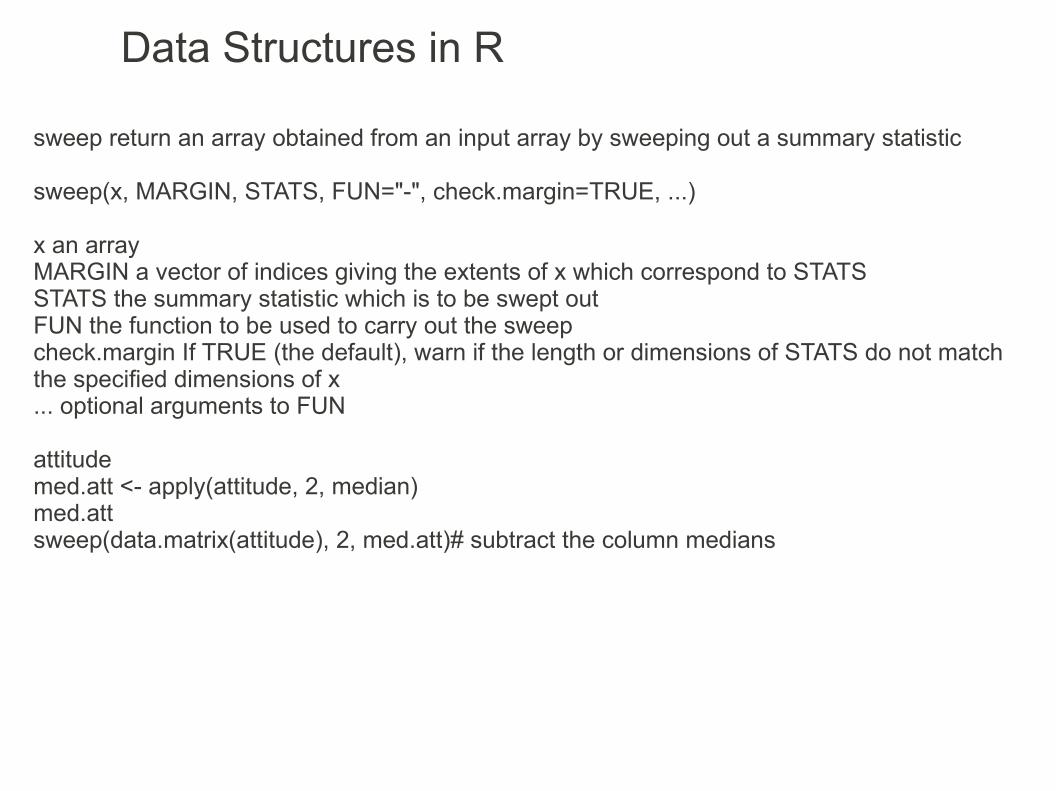
Data Structures in R
sweep return an array obtained from an input array by sweeping out a summary statistic
sweep(x, MARGIN, STATS, FUN="-", check.margin=TRUE, ...)
x an arrayMARGIN a vector of indices giving the extents of x which correspond to STATSSTATS the summary statistic which is to be swept outFUN the function to be used to carry out the sweepcheck.margin If TRUE (the default), warn if the length or dimensions of STATS do not match the specified dimensions of x... optional arguments to FUN
attitudemed.att <- apply(attitude, 2, median)med.attsweep(data.matrix(attitude), 2, med.att)# subtract the column medians

Data Structures in RAttach a set of R objects to the search path
attach(what, pos = 2, name = deparse(substitute(what)), warn.conflicts = TRUE)
Argumentswhat a data.frame, list, R data file or an environmentpos position in search() where to attach name name to use for the attached database warn.conflicts if true then it shows conflicts from attaching the database
Objects on what will be accessible directly through their names

Data Structures in R
mydataf <- data.frame(age=c(25,22,26,28),height=c(174,166,174,170),weight=c(75,55,60,60),city=c("Turku","Espoo","Kuopio","Helsinki"),row.names =c("Pekka","Anna","Ari","Tove"))mydatafls()search()attach(mydataf)ls()search()detach(mydataf)ls()search()rm(mydataf)ls()search()

Data Structures in R> mydataf <- data.frame(age=c(25,22,26,28),height=c(174,166,174,170),weight=c(75,55,60,60),city=c("Turku","Espoo","Kuopio","Helsinki"),row.names =c("Pekka","Anna","Ari","Tove"))> ls()[1] "mydataf"> search()[1] ".GlobalEnv" "package:stats" "package:graphics" [4] "package:grDevices" "package:utils" "package:datasets" [7] "package:methods" "Autoloads" "package:base" > attach(mydataf)> ls()[1] "mydataf"> search() [1] ".GlobalEnv" "mydataf" "package:stats" [4] "package:graphics" "package:grDevices" "package:utils" [7] "package:datasets" "package:methods" "Autoloads" [10] "package:base" > detach(mydataf)> ls()[1] "mydataf"> search()[1] ".GlobalEnv" "package:stats" "package:graphics" [4] "package:grDevices" "package:utils" "package:datasets" [7] "package:methods" "Autoloads" "package:base" > rm(mydataf)> ls()character(0)> search()[1] ".GlobalEnv" "package:stats" "package:graphics" [4] "package:grDevices" "package:utils" "package:datasets" [7] "package:methods" "Autoloads" "package:base"
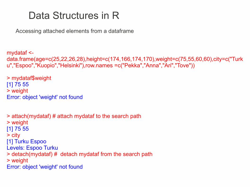
Data Structures in R
mydataf <- data.frame(age=c(25,22,26,28),height=c(174,166,174,170),weight=c(75,55,60,60),city=c("Turku","Espoo","Kuopio","Helsinki"),row.names =c("Pekka","Anna","Ari","Tove"))
> mydataf$weight[1] 75 55> weightError: object 'weight' not found
> attach(mydataf) # attach mydataf to the search path> weight[1] 75 55> city[1] Turku EspooLevels: Espoo Turku> detach(mydataf) # detach mydataf from the search path> weightError: object 'weight' not found
Accessing attached elements from a dataframe

Data Structures in RAccessing attached elements from a dataset
data()ToothGrowthnames(ToothGrowth) # len supp dosesupp # errorToothGrowth$suppattach(ToothGrowth)suppdetach(ToothGrowth)supp

Data Structures in RReferences/to learn more:
The R bookMichael J. Crawley pp 152012 John Wiley & Sons Ltd
Basic statistics using R pp. 40Jarno Tuimala (CSC) and Dario Greco (HY)http://www.csc.fi/english/csc/courses/archive/R2008s
Statistics: an introduction using RMichael J. Crawley pp 2882010 John Wiley & Sons Ltd
Statistics with RVincent Zoonekynd, pp 34http://zoonek2.free.fr/UNIX/48_R/all.html
Aprendizaje del software estadístico R: un entorno para simulación y computación estadísticaProf. Alberto muñoz garcíaDepartamento de EstadísticaUniversidad Carlos III de Madridhttp://ocw.uc3m.es/estadistica/aprendizaje-del-software-estadistico-r-un-entorno-para-simulacion-y-computacion-estadistica/resolveUid/a30d9f0c6a5ca66fdee17e6088a070ad
Introductory Statistics with RPeter Dalgaard, pp 112013 Springer
Software Tools, Part 1: introduction to R softwarePetri Koistinenhttp://www.rni.helsinki.fi/~pek/s-tools/vectors.r
Quick-RRob Kabacoffhttp://www.statmethods.net/input/datatypes.html
The Stem and Tendril simplified R manualProfessors Franzblau, Poje and Verzani of the College of Staten Islandhttp://wiener.math.csi.cuny.edu/st/stRmanual/

Displaying data on Rdir() and list.files() lists the files in a directory
list.files(path = ".", pattern = NULL, all.files = FALSE, full.names = FALSE, recursive = FALSE, ignore.case = FALSE)
dir(path = ".", pattern = NULL, all.files = FALSE, full.names = FALSE, recursive = FALSE, ignore.case = FALSE)
path vector of full path names; the default is the working directory getwd()pattern match an optional regular expression. Not wildcards!all.files If TRUE, all file names will be returned, even hidden and system files or not visible for other reasonfull.names If TRUE, the directory path is prepended to the file namesrecursive logical If TRUE, the listing will recurse into sub-directoriesignore.case If TRUE, the search will be case-insensitive. It's always case-insensitive on Windows
Note:
R.home() # the path of R's home directory

Displaying data on R
dir()list.files() dir(pattern="^a") # list all files that start with "a"dir(pattern="\\.R$") # list all files that end with ".R"list.files(path = "c:/temp") # list all files from c:\templist.files(path = "c:/temp", all.files =TRUE) # list all files from c:\temp, even not visible files

file.show() display one or more files, usually text files
file.show(..., header = rep("", nfiles), title = "R Information", delete.file = FALSE, pager = getOption("pager"), encoding = "")
... one or more character vectors containing the names of the filesheader character vector (of the same length as the number of files specified in ...) giving a header for each filetitle an overall title for the displaydelete.file should the files be deleted after display? Used for temporary filespager the pager to be usedencoding character string giving the encoding to be assumed for the file(s)
dir()file.show(".Rhistory")
Displaying data on R

Displaying data on Rprint displays values, expressions or variables
print(123) # displaying a numberprint("abc") # displaying a stringprint(123+567) # displaying an expression
cat concatenates and outputs objectsBy default it will output to the Console (screen)
cat(... , sep = " ", fill = FALSE, labels = NULL)
... R objectssep a character vector of strings to append after each elementfill a logical or (positive) numeric controlling how the output is broken into successive lines. If FALSE (default), only newlines created explicitly by "\n" are printed. Otherwise, the output is broken into lines with print width equal to the option width if fill is TRUE, or the value of fill if this is numeric. Non-positive fill values are ignored, with a warning. labels character vector of labels for the lines printed. Ignored if fill is FALSE.
cat(5,"*",12,"=",5*12,"\n")cat(5,"*",12,"=",5*12,"\n", sep = "_")cat(5,"*",12,"=",5*12,"\n", sep = " ")cat(rep("0123456789",20), fill = T, width=3, labels = c("line 1","line 2","line 3","line 4"))

Displaying data on R
paste concatenate vectors to strings
paste(..., sep = " ", collapse = NULL)
... one or more R objects, to be converted to character vectorssep a character string to separate the terms. Not NA_character_collapse an optional character string to separate the results. Not NA_character_
paste(1:3) # same as as.character(1:3)paste(1:3,sep = "") # separate terms - only 1 term, nothing to dopaste(c("one","two","three"))paste(c("one","two","three"), sep = "")# separate terms - only 1 term, nothing to dopaste(c("one","two","three"), collapse="***") # separate results OK
paste(1,2,3)paste(1,2,3,sep = "") # separate terms OKpaste("one","two","three")paste("one","two","three", sep = "") # separate terms OKpaste("one","two","three", collapse="***") # separate results - only 1 result, nothing to do
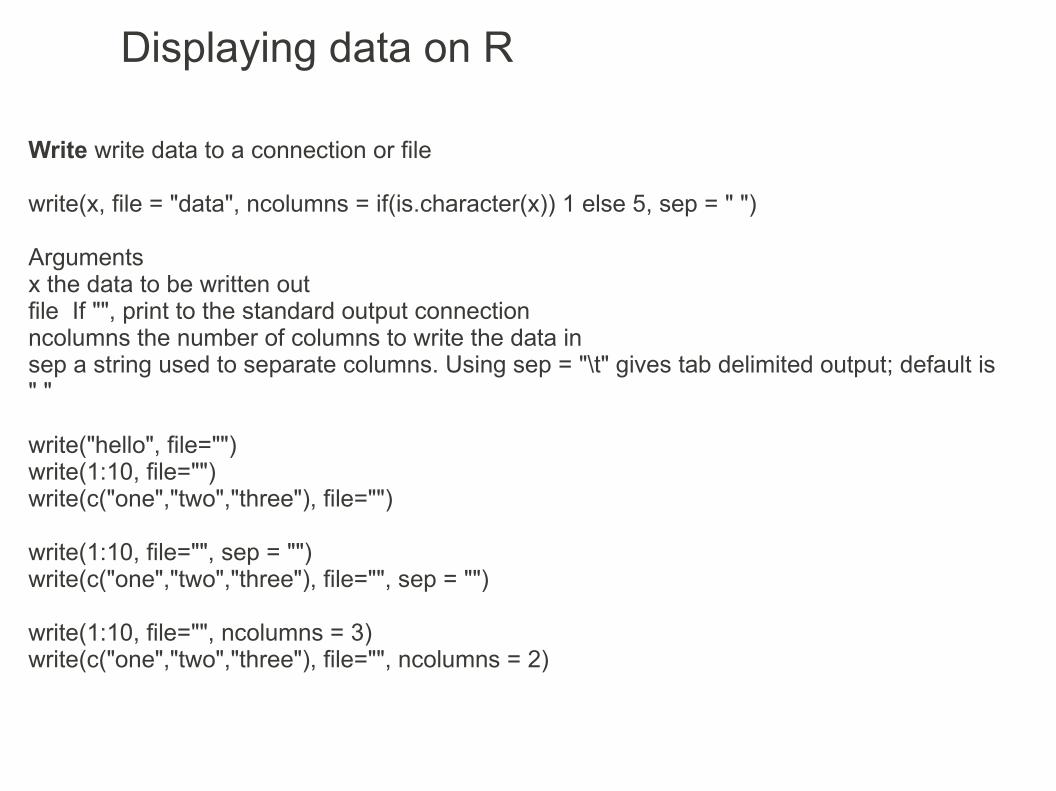
Displaying data on R
Write write data to a connection or file
write(x, file = "data", ncolumns = if(is.character(x)) 1 else 5, sep = " ")
Argumentsx the data to be written outfile If "", print to the standard output connectionncolumns the number of columns to write the data insep a string used to separate columns. Using sep = "\t" gives tab delimited output; default is " "
write("hello", file="")write(1:10, file="")write(c("one","two","three"), file="")
write(1:10, file="", sep = "")write(c("one","two","three"), file="", sep = "")
write(1:10, file="", ncolumns = 3)write(c("one","two","three"), file="", ncolumns = 2)

sink redirects R output to a connection
sink.number() displays the number of current redirections
sink(file = NULL, append = FALSE, type = c("output", "message"), split = FALSE)
sink.number(type = c("output", "message"))
file a connection or a file name or NULL to stopappend If TRUE, output will be appended, otherwise, it will be overwrittentype either output stream or the messages streamsplit if TRUE, output will be sent to both new and old streams
sink("output.txt") # creates a file to store the output# the output will now be sent to file "output.txt"print("Hello world!")print(123*pi)sink() # stop sending the output to the file
Redirecting data on R

edit invokes a text editor on an R object
edit(name = NULL, file = "", title = NULL, editor = getOption("editor"), ...)
vi(name = NULL, file = "")emacs(name = NULL, file = "")pico(name = NULL, file = "")xemacs(name = NULL, file = "")xedit(name = NULL, file = "")
name R object or file name to editfile file nametitle a title for the objecteditor text editor to use... further arguments to be passed to or from methods
Editing data on R
Invoking a specific editor

# open a filedir()edit(file="output.txt")
v1 <- c(734, 985, 43, 952)v2 <- c("Helsinki","Tampere","Turku")v3 <- c(T,F,F,F,T,F,T,F,T,T)myarray<-array(c(56,67,174,166,75,55,77,70,64,77,178,170,78,59,63,61),c(2,4,2))dimnames(myarray) = list(c("men","women"),c("age","height","weight","pulse"), c("city","countryside"))mydataf <- data.frame(age=c(25,22,26,28),height=c(174,166,174,170),weight=c(75,55,60,60),city=c("Turku","Espoo","Kuopio","Helsinki"),row.names =c("Pekka","Anna","Ari","Tove"))mymatrix <- matrix(1:6*10,3,2)
# open the R Editor with the code to define the variablesedit(v1)edit(v2)edit(v3)edit(myarray)
# open the R Data Editoredit(mydataf)edit(mymatrix)
Editing data on R

Editing data on R
Fix an R object
fix invokes edit on x and then updates x in the user's workspace
fix(x, ...)
x the name of an R object... arguments to pass to edit

> mymatrix <- matrix(1:6*10,3,2)> mymatrix [,1] [,2][1,] 10 40[2,] 20 50[3,] 30 60> edit(mymatrix) col1 col2[1,] 10 40[2,] 20 50[3,] 30 60[4,] 55 66> mymatrix [,1] [,2][1,] 10 40[2,] 20 50[3,] 30 60> fix(mymatrix)> mymatrix col1 col2[1,] 10 40[2,] 20 50[3,] 30 60[4,] 55 77
Editing data on R

Data input on R
> mydata1 <- scan()1: 12: 23: 34: Read 3 items> mydata1 [1] 1 2 3> is(mydata1)[1] "numeric" "vector" > mydata1 <- scan()1: 1 2 34: Read 3 items> mydata1 [1] 1 2 3> is(mydata1)[1] "numeric" "vector"
Reading input from the console
Type1 Enter 2 Enter 3 Enter Enter
Type1 Space 2 Space 3 Enter Enter
Same input

Data input on R
> mydata1 <- scan()1: a1: bError in scan(file, what, nmax, sep, dec, quote, skip, nlines, na.strings, : scan() expected 'a real', got 'a'
Trying to enter text as input:
The default input data type is numeric, solution: use the what argument
Useful arguments for console input
what input data type logical, integer, numeric, complex, character
nmax maximum number of input values
nlines maximum number of lines of data
na.strings vector of elements interpreted as missing (NA) values

Data input on R
> mydata1 <- scan(what=character())1: a b c4: Read 3 items> mydata1 [1] "a" "b" "c"> mydata1 <- scan(what=character())1: "one two" "three four"3: Read 2 items> mydata1 [1] "one two" "three four"
what input data type logical, integer, numeric, complex, character
> mydata1 <- scan(what=logical())1: T2: F3: TRUE4: FALSE5: Read 4 items> mydata1 [1] TRUE FALSE TRUE FALSE
> mydata1 <- scan()1: 25*pi1: 15Error in scan(file, what, nmax, sep, dec, quote, skip, nlines, na.strings, : scan() expected 'a real', got '25*pi'> mydata1 <- scan()1: sqrt(2)1: 5Error in scan(file, what, nmax, sep, dec, quote, skip, nlines, na.strings, : scan() expected 'a real', got 'sqrt(2)'
> mydata1 <- scan(what=complex())1: -6576.98982: 3.54i3: -5.543-.68767i4: Read 3 items> mydata1 [1] -6576.990+0.00000i 0.000+3.54000i -5.543-0.68767i
Quotes allow space on strings
Constants and functions are not allowed
5i and 5*i are not the same
Logical will not accept 1 or 0

Data input on R
nmax maximum number of input values
nlines maximum number of lines of data
> mydata1 <- scan(nmax=4)1: 92: 83: 74: 6Read 4 items> mydata1[1] 9 8 7 6> mydata1 <- scan(nmax=4)1: 22 33 44 55 66 77 88 99Read 4 items> mydata1[1] 22 33 44 55
> mydata1 <- scan(nlines=4)1: 112: 223: 334: 44Read 4 items> mydata1[1] 11 22 33 44> mydata1 <- scan(nlines=4)1: 1 2 3 4 5 6 7 89: 99 88 7712: 66 55 4415: 33 22 11Read 17 items> mydata1 [1] 1 2 3 4 5 6 7 8 99 88 77 66 55 44 33 22 11
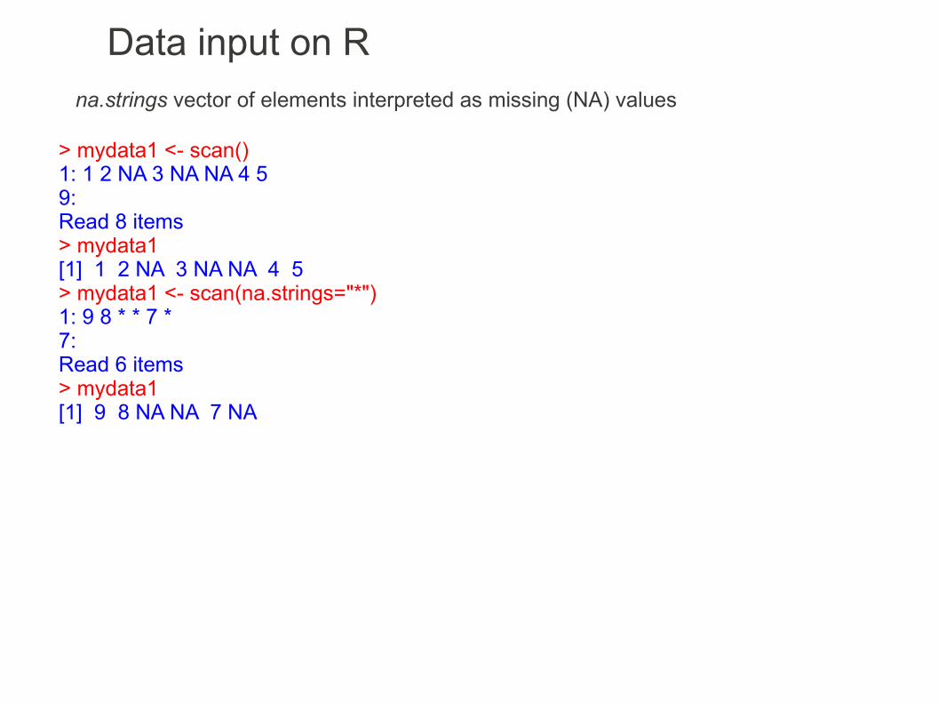
Data input on Rna.strings vector of elements interpreted as missing (NA) values
> mydata1 <- scan()1: 1 2 NA 3 NA NA 4 59: Read 8 items> mydata1[1] 1 2 NA 3 NA NA 4 5> mydata1 <- scan(na.strings="*")1: 9 8 * * 7 *7: Read 6 items> mydata1[1] 9 8 NA NA 7 NA

Data input on RReading input from the the web
# read a text file from the web to a stringcon <- url("http://www.rni.helsinki.fi/~pek/r-koulutus/e2.dat") # open a connectionmytxt <- readLines(con) # read the fileclose(con) # close the connectionmytxt
# execute code from the websource("http://www.rni.helsinki.fi/~pek/r-koulutus/hello.R")
# download a file from the webdownload.file("http://www.rni.helsinki.fi/~pek/r-koulutus/hello.R",destfile="hello.R")download.file("http://www.rni.helsinki.fi/~pek/r-koulutus/e2.dat",destfile="e2.dat")dir() # show the files on the working directory
# reading a data frame from the webmydf <- read.table(url('http://www.rni.helsinki.fi/~pek/s-tools/e1.dat'))mydfclass(mydf)

Data input on RReading input from a file
Comma-separated values (CSV) filesText files containing data, each line of text is a row (record) of data and within each line, each column (field) of data is separated by a comma. Usually the first line has the column names.
Rules
●Records are separated by end-of-line characters●Fields are separated by commas●Leading or trailing spaces are part of the field data●Commas within fields are enclosed with double-quotes●double-quotes within fields are replaced by a pair of double-quotes●The first line might have the column names
Exceptions
●Line breaks can be placed inside double quotes●If the comma is used as a decimal sign then semicolons will separate the columns●Some implementations remove leading or trailing spaces●Some implementations enclose fields with leading or trailing spaces, within double-quotes●Some implementations enclose all fields within double-quotes
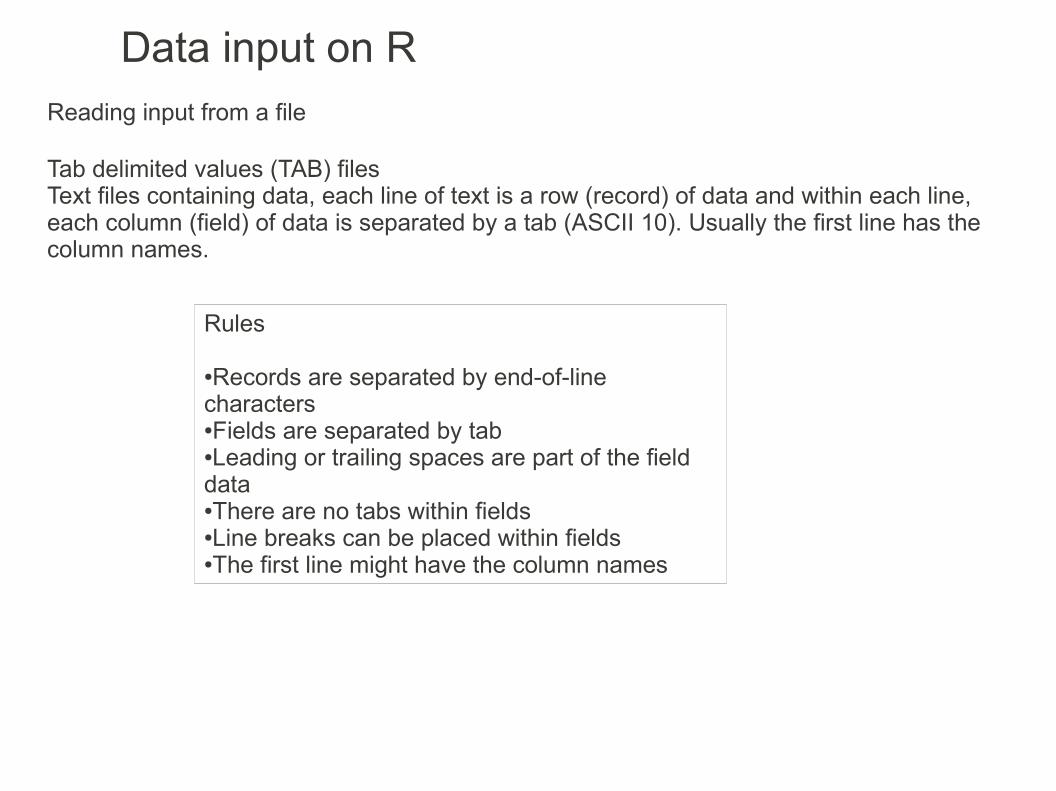
Data input on RReading input from a file
Tab delimited values (TAB) filesText files containing data, each line of text is a row (record) of data and within each line, each column (field) of data is separated by a tab (ASCII 10). Usually the first line has the column names.
Rules
●Records are separated by end-of-line characters●Fields are separated by tab●Leading or trailing spaces are part of the field data●There are no tabs within fields●Line breaks can be placed within fields●The first line might have the column names

Data input on RReading input from a file
Fixed Width Text FilesText files containing data, each line of text is a row (record) of data and within each line, each column (field) of data has a constant, pre-defined number of characters. Usually the first line has the column names.
Rules
●Records are separated by end-of-line characters●Fields have a fixed size●Leading or trailing spaces are used as padding, unless anothe character is chosen for that purpose●Line breaks can be placed within fields●The first line might have the column names

Data input on RReading input from a file
File "hello.R" from the previous example should be on the working directory, "e2.dat" too.
# To read and execute it:source("hello.R")# To open a window for choosing a file to open:source( file.choose() )
# read a text file from a file to a stringcon <- file("e2.dat") # open a connectionmytxt <- readLines(con) # read the fileclose(con) # close the connectionmytxt

Data input on RReading input from a file
scan()
Useful arguments for file input
what input data type logical, integer, numeric, complex, character, list
nmax maximum number of input values
nlines maximum number of lines of data
na.strings vector of elements interpreted as missing (NA) values
sep character that delimits fields, the default is white-space or end-of-line (unless within quotes)
dec decimal point character because of "." vs ","
skip the number of lines to skip from the beginning of the file
blank.lines.skip if true then blank lines are skipped
comment.char a character that marks comment lines, which are skipped

Data input on RReading input from a file
> mytxt <- scan("e2.dat") # read the fileError in scan(file, what, nmax, sep, dec, quote, skip, nlines, na.strings, : scan() expected 'a real', got '#'
> mytxt <- scan("e2.dat", skip=2) # read the file, skip the 1st 2 linesRead 14 items> mytxt [1] 46 148 54 182 48 173 50 166 44 109 42 141 52 166
> mytxt <- scan("e2.dat", what = list("",""), skip=2)Read 7 records> mytxt [[1]][1] "46" "54" "48" "50" "44" "42" "52"
[[2]][1] "148" "182" "173" "166" "109" "141" "166"

Data input on RReading input from a file
sep character that delimits fields, the default is white-space or end-of-line (unless within quotes)
blank.lines.skip if true then blank lines are skipped
comment.char a character that marks comment lines, which are skipped
> cat("12:34:56:78:90",file="numbers.txt") # create a text file with text "12:34:56:78:90"> edit(file="numbers.txt")> mytxt <- scan("numbers.txt", sep=":") # read the fileRead 5 items> mytxt[1] 12 34 56 78 90> > cat("12:34\n56:78:90",file="numbers.txt") # end-of-line also works> edit(file="numbers.txt")> mytxt <- scan("numbers.txt", sep=":") # read the fileRead 5 items> mytxt[1] 12 34 56 78 90
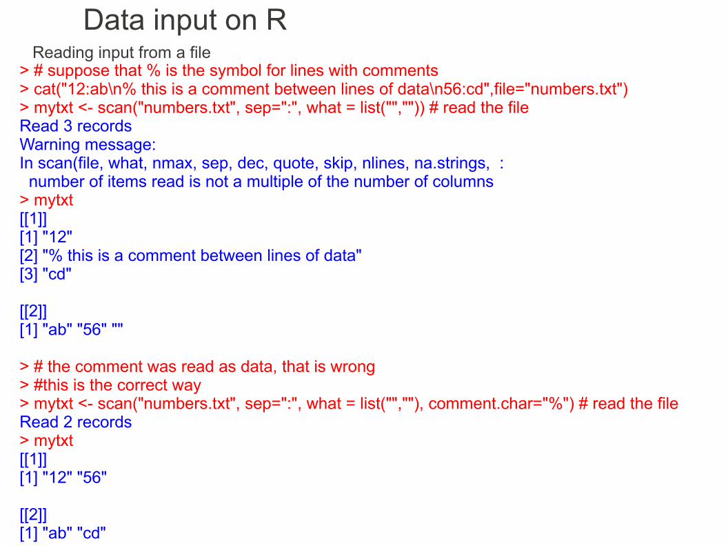
Data input on RReading input from a file
> # suppose that % is the symbol for lines with comments> cat("12:ab\n% this is a comment between lines of data\n56:cd",file="numbers.txt")> mytxt <- scan("numbers.txt", sep=":", what = list("","")) # read the fileRead 3 recordsWarning message:In scan(file, what, nmax, sep, dec, quote, skip, nlines, na.strings, : number of items read is not a multiple of the number of columns> mytxt[[1]][1] "12" [2] "% this is a comment between lines of data"[3] "cd"
[[2]][1] "ab" "56" ""
> # the comment was read as data, that is wrong > #this is the correct way> mytxt <- scan("numbers.txt", sep=":", what = list("",""), comment.char="%") # read the fileRead 2 records> mytxt[[1]][1] "12" "56"
[[2]][1] "ab" "cd"
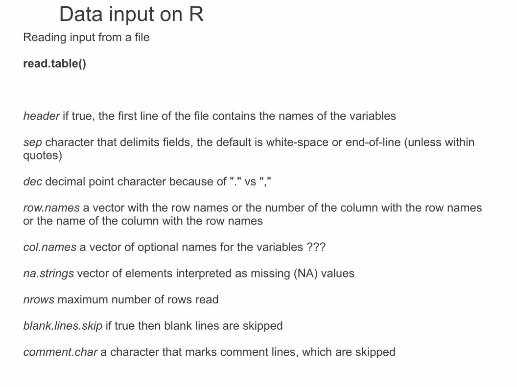
Data input on RReading input from a file
read.table()
header if true, the first line of the file contains the names of the variables
sep character that delimits fields, the default is white-space or end-of-line (unless within quotes)
dec decimal point character because of "." vs ","
row.names a vector with the row names or the number of the column with the row names or the name of the column with the row names
col.names a vector of optional names for the variables ???
na.strings vector of elements interpreted as missing (NA) values
nrows maximum number of rows read
blank.lines.skip if true then blank lines are skipped
comment.char a character that marks comment lines, which are skipped

Data input on RReading input from a file
read.table() Reads a text file in table format and creates a data frame from it
read.csv(file, header = TRUE, sep = ",", quote="\"", dec=".", fill = TRUE, comment.char="", ...)
read comma separated value files (CSV)
read.csv2(file, header = TRUE, sep = ";", quote="\"", dec=",", fill = TRUE, comment.char="", ...)
CSV with comma as decimal point and a semicolon as field separator
read.delim(file, header = TRUE, sep = "\t", quote="\"", dec=".", fill = TRUE, comment.char="", ...)
read TAB delimited files (TAB)
read.delim2(file, header = TRUE, sep = "\t", quote="\"", dec=",", fill = TRUE, comment.char="", ...)
TAB with comma as decimal point
read.fwf(file, widths, header = FALSE, sep = "\t", skip = 0, row.names, col.names, n = -1, buffersize = 2000, ...)
read a table of fixed width formatted data
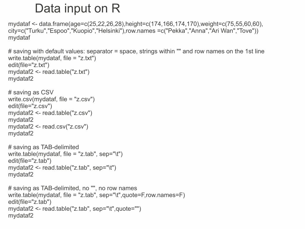
mydataf <- data.frame(age=c(25,22,26,28),height=c(174,166,174,170),weight=c(75,55,60,60), city=c("Turku","Espoo","Kuopio","Helsinki"),row.names =c("Pekka","Anna","Ari Wan","Tove"))mydataf
# saving with default values: separator = space, strings within "" and row names on the 1st linewrite.table(mydataf, file = "z.txt")edit(file="z.txt")mydataf2 <- read.table("z.txt")mydataf2
# saving as CSVwrite.csv(mydataf, file = "z.csv")edit(file="z.csv")mydataf2 <- read.table("z.csv")mydataf2mydataf2 <- read.csv("z.csv")mydataf2
# saving as TAB-delimitedwrite.table(mydataf, file = "z.tab", sep="\t")edit(file="z.tab")mydataf2 <- read.table("z.tab", sep="\t")mydataf2
# saving as TAB-delimited, no "", no row nameswrite.table(mydataf, file = "z.tab", sep="\t",quote=F,row.names=F)edit(file="z.tab")mydataf2 <- read.table("z.tab", sep="\t",quote="")mydataf2
Data input on R

Data input on Rread.ftable(), write.ftable() read, write "flat" contingency tables
Usageread.ftable(file, sep = "", quote = "\"", row.var.names, col.vars, skip = 0)
write.ftable(x, file = "", quote = TRUE, append = FALSE, digits = getOption("digits"))
file either a character string naming a file or a connection which the data are to be read from or written to
sep character that delimits fields, the default is white-space or end-of-line (unless within quotes)
quote a character string giving the set of quoting characters for read.ftable
row.var.names a character vector with the names of the row variables
col.vars a list giving the names and levels of the column variables
skip the number of lines of the data file to skip before beginning to read data x an object of class "ftable" append If TRUE, the output from write.ftable is appended to the file digits an integer giving the number of significant digits

Data input on R
Write an object to a file in ASCII format or read an object from a file
dget() and dput()
dget(filename) reads an R object from file "filename"dput(obj, filename) writes an object "obj" to a file "filename", in ASCII format
> mydataf <- data.frame(age=c(25,22),height=c(174,166),weight=c(75,55), city=c("Turku","Espoo"),row.names =c("Pekka","Anna"))> dput(mydataf,"mydf.dat")> mydataf2 <- dget("mydf.dat")> mydataf2 == mydataf age height weight cityPekka TRUE TRUE TRUE TRUEAnna TRUE TRUE TRUE TRUE

dump(list, file = "dumpdata.R", append = FALSE, control = "all", envir = parent.frame(), evaluate = TRUE)
list vector wi names of one or more R objects to be dumped. file either a character string naming a file or a connection. "" indicates output to the console. append if TRUE and file is a character string, output will be appended to file; otherwise, it will overwrite the contents of file.
source() reads R code from a file or a connection
source(file, local = FALSE, echo = verbose, print.eval = echo, verbose = getOption("verbose"), prompt.echo = getOption("prompt"), max.deparse.length = 150, chdir = FALSE, encoding = getOption("encoding"), continue.echo = getOption("continue"), skip.echo = 0, keep.source = getOption("keep.source"))
file a connection or a character string giving the pathname of the file or URL to read fromecho if TRUE, each expression is printed after parsing, before evaluationprint.eval if TRUE, the result of eval(i) is printed for each expression i; defaults to the value of echoverbose if TRUE, more diagnostics (than just echo = TRUE) are printed during parsing and evaluation of input, including extra info for each expressionprompt.echo character; gives the prompt to be used if echo = TRUEencoding The encoding(s) to be assumed when file is a character string: see fileskip.echo if echo = TRUE, how many lines to skip from the beginning
Data input on R

Data input on R
a <- 543.86dump(a, "test_a.R") # error!dump(ls(pattern ="a"), "test_a.R") # works...dir(pattern="test")ls()rm(a)als()source("test_a.R")als()
# to choose a file interactively:source(file.choose())

Data input on R
mydataf <- data.frame(age=c(25,22,26,28),height=c(174,166,174,170),weight=c(75,55,60,60),city=c("Turku","Espoo","Kuopio","Helsinki"),row.names =c("Pekka","Anna","Ari","Tove"))dump(ls("mydataf"), file ="test_mydataf.R") # error!ls()search()attach(mydataf)ls()search()dump(ls("mydataf"), file ="test_mydataf.R")dir(pattern="test")detach(mydataf)rm(mydataf)ls()search()source("test_mydataf.R")ls()search() # "age" "city" "height" "weight"!mydataf # got attached!edit(file="test_mydataf.R") # this is why!

Write write data to a connection or file
write(x, file = "data", ncolumns = if(is.character(x)) 1 else 5, sep = " ")
Argumentsx the data to be written outfile If "", print to the standard output connectionncolumns the number of columns to write the data insep a string used to separate columns. Using sep = "\t" gives tab delimited output; default is " "
write("hello", file="hello.txt")write(1:10, file="1to10.txt")write(c("one","two","three"), file="123.txt")
write(1:10, file="1to10b.txt", sep = "")write(c("one","two","three"), file="123b.txt", sep = "")
write(1:10, file="1to10c.txt", ncolumns = 3)write(c("one","two","three"), file="123c.txt", ncolumns = 2)
myvector<-c(1,2,3,4,5)write(myvector,"myvector.txt")
mymatrix<-matrix(1:9,ncol=3,byrow=T)write(t(mymatrix),"mymatrix.txt",ncol=ncol(mymatrix))
Data input on R

cat concatenates and outputs objects, also to a fileBy default it will output to the Console (screen)
cat(... , file = "", sep = " ", fill = FALSE, labels = NULL, append = FALSE)
... R objectsfile file name to get the outputsep a character vector of strings to append after each elementfill a logical or (positive) numeric controlling how the output is broken into successive lines. If FALSE (default), only newlines created explicitly by "\n" are printed. Otherwise, the output is broken into lines with print width equal to the option width if fill is TRUE, or the value of fill if this is numeric. Non-positive fill values are ignored, with a warning. labels character vector of labels for the lines printed. Ignored if fill is FALSE. append if TRUE, the outpur is appended at the end of the file
cat("Hello world!", file = "cattest.txt")edit(file="cattest.txt")cat("Hello aliens!", file = "cattest.txt", append = TRUE)edit(file="cattest.txt")
Data input on R

Data input on Rsave() saves R objects
save(..., list = character(0L), file = stop("'file' must be specified"), ascii = FALSE, version = NULL, envir = parent.frame(), compress = !ascii, eval.promises = TRUE, precheck = TRUE)
... the names of the objects to be savedlist A vector containing the names of objects to be savedfile a connection or the name of the file where the data will be savedascii if TRUE, an ASCII representation of the data is written compress if TRUE, the filr is compressedprecheck if TRUE, the existence of the objects is checked before saving
load() loads datasets saved with save()
v1 <- c(734, 985, 43, 952)v2 <- c("Helsinki","Tampere","Turku") save(v1, v2, file = "v1v2.Rdata")#remove all objectsrm(list=ls(all=TRUE))v1;v2load("v1v2.Rdata")v1;v2save(v1, v2, file = "v1v2.Rdata", ascii = TRUE)edit(file="v1v2.Rdata")

Data input on RReferences/to learn more:
The R bookMichael J. Crawley pp 972014 John Wiley & Sons Ltd
Basic statistics using R pp. 57Jarno Tuimala (CSC) and Dario Greco (HY)http://www.csc.fi/english/csc/courses/archive/R2008s
Statistics: an introduction using RMichael J. Crawley pp 2862012 John Wiley & Sons Ltd
Statistics with RVincent Zoonekynd, pp 91http://zoonek2.free.fr/UNIX/48_R/all.html
Aprendizaje del software estadístico R: un entorno para simulación y computación estadísticaProf. Alberto muñoz garcíaDepartamento de EstadísticaUniversidad Carlos III de Madridhttp://ocw.uc3m.es/estadistica/aprendizaje-del-software-estadistico-r-un-entorno-para-simulacion-y-computacion-estadistica/resolveUid/81279218bad3be4326b943c4c3e62e4d
Introductory Statistics with RPeter Dalgaard, pp 462014 Springer
Software Tools, Part 1: introduction to R softwarePetri Koistinenhttp://www.rni.helsinki.fi/~pek/s-tools/data-input.r
Quick-RRob Kabacoffhttp://www.statmethods.net/input/index.html
The Stem and Tendril simplified R manualProfessors Franzblau, Poje and Verzani of the College of Staten Islandhttp://wiener.math.csi.cuny.edu/st/stRmanual/
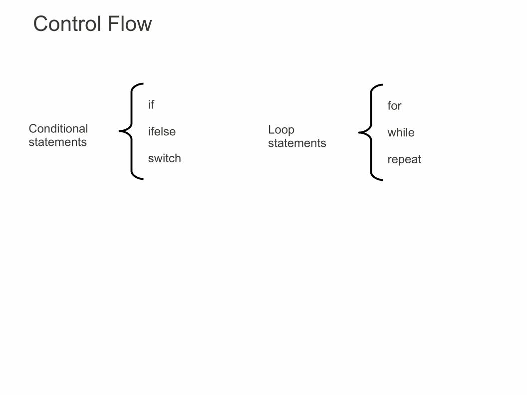
Control Flow
Conditional statements
if
ifelse
switch
Loop statements
for
while
repeat

if - Conditional statement
if(condition) expression # if the condition is true then the expression will executeif(condition) expression else alternate.expression # if the condition is true then the expression will execute, otherwise the alternate.expression will execute
condition - a logical result, not NA. Only the first element of a vector is considered.expression, alternate.expression - Either a simple expression, one command only, or a so called compound expression { expression1 ; expression2 } or:{expression1expression2}
To separate several expressions can be done with ; or newline but newline is more clear and understandable.A newline before an else statement will cause an error.
> if (5 > 3) print ("OK") # this always returns "OK"[1] "OK"
Control Flow

# get a random integer number from 1 to 10, say if it is greater than 5 or notif (sample(1:10, 1) > 5) print ("random number > 5") else print ("random number < 5")
# same as above but in separate lines of codeif (sample(1:10, 1) > 5) print ("random number > 5") else print ("random number < 5")
# get a random integer number from 1 to 10, if greater than 5 then show its square value# otherwise show it multiplied by 4myrnd <- sample(1:10, 1)if (myrnd > 5) {myrnd2 <- myrnd^2;print (myrnd2)} else {myrnd2 <- myrnd*4;print (myrnd2)}
# same as above but in separate lines of codemyrnd <- sample(1:10, 1)if (myrnd > 5){ myrnd2 <- myrnd^2 print (myrnd2)} else{ myrnd2 <- myrnd*4 print (myrnd2)}
This code should be tested on the R editor, selecting a block if code + ctrl r
Control Flow

"If" can be used as a function within expressions:
> x <- 5> strwhartx <- if(is.complex(x)) "imaginary" else "real"> strwhartx [1] "real"
Control Flow

Conditional Element Selection
Ifelse - returns 1 out of 2 elements, depending on a logical condition.
ifelse(condition, condition.true.expression, condition.false.expression)
> x <- 5-7i> ifelse(is.complex(x), "imaginary", "real") # if x is complex, return "imaginary", otherwise "real"[1] "imaginary"> x <- 16> ifelse(is.complex(x), "imaginary", "real") # if x is complex, return "imaginary", otherwise "real"[1] "real"
Control Flow

Control FlowIfelse on multiple elements
Ifelse can affect elements from vectors, matrices, etc... directly, with no need for loops or for "apply" functions
# get the sign (-1, 0, 1) from numbers> ifelse(myvec >0, 1, ifelse(myvec <0, -1, 0))[1] -1 -1 -1 0 1 1 1
# replace numbers with a word# NA MISSING# Inf INFINITY# >0 POSITIVE# <0 NEGATIVE# =0 ZEROmyvec <- c(-3:3, Inf, NA)myvecmyvec <- sample(myvec) # random permutationmyvecmyvec.str <- ifelse(is.na(myvec),"MISSING",
ifelse(is.infinite(myvec),"INFINITY",ifelse(myvec>0,"POSITIVE",
ifelse(myvec<0,"NEGATIVE","ZERO"
))))myvec.str
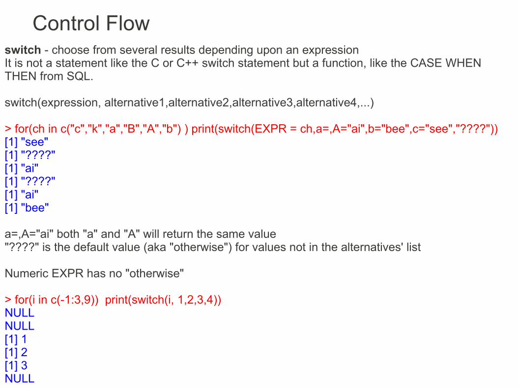
Control Flowswitch - choose from several results depending upon an expressionIt is not a statement like the C or C++ switch statement but a function, like the CASE WHEN THEN from SQL.
switch(expression, alternative1,alternative2,alternative3,alternative4,...)
> for(ch in c("c","k","a","B","A","b") ) print(switch(EXPR = ch,a=,A="ai",b="bee",c="see","????"))[1] "see"[1] "????"[1] "ai"[1] "????"[1] "ai"[1] "bee"
a=,A="ai" both "a" and "A" will return the same value"????" is the default value (aka "otherwise") for values not in the alternatives' list
Numeric EXPR has no "otherwise"
> for(i in c(-1:3,9)) print(switch(i, 1,2,3,4))NULLNULL[1] 1[1] 2[1] 3NULL

Control Flowfor
for (var in seq) exprbreaknext
for will cycle throught the elements of a vector sequentially until it reaches the last element or the break command is found within the loop. Next skips the current iteration.
> for(i in 4:7) print(i)[1] 4[1] 5[1] 6[1] 7> for(i in c(734, 985, 43, 952)) print(i)[1] 734[1] 985[1] 43[1] 952> for(i in c("Helsinki","Tampere","Turku")) print(i)[1] "Helsinki"[1] "Tampere"[1] "Turku"
Loop through a sequence of numbers
Loop through a vector of numbers
Loop through a vector of strings

Control Flow
> for(i in 1:10) + {+ print(i)+ if (i==3) break+ }[1] 1[1] 2[1] 3> > for(i in 1:10) + {+ if (i/2==i %/%2) next+ print(i)+ }[1] 1[1] 3[1] 5[1] 7[1] 9
next skips the current iteration
All the even numbers are skipped
break exits the loop

Control Flow
while
while(cond) exprbreaknext
while will test a condition and execute an expression if the condition is TRUE, then it will test the condition again and so forth.
break exits the loopnext skips the current iteration, it will cause an infinite loop unless the variable is updated before the next statement

Control Flow# example of using whilen <- 1while (n < 5){print(n)n <- n+1}# example of using while and nextn <- 0while ((n <- n+1) < 5){if (n==2) nextprint(n)}# example of using while and nextn <- 0while (n < 5){n <- n+1if (n==2) nextprint(n)}# example of using while and breakn <- 1while (n < 5){if (n==2) breakprint(n)n <- n+1}
The code before next is executedThe code after next is skipped
The code before break is executedThe code after break is skipped and the loop ends
The code before next is executedThe code after next is skipped
The loop variable must be updated before reaching the next, otherwise the loop will be infinite

Control Flowprint("Game: I will choose 3 numbers between 1 and 8, you have to guess them to win this game")x <- sample(1:8,3)user.score <- c()while (length(x)>0){print("Give me a number between 1 and 8")user.try <- scan(,what=numeric(),1)if (user.try %in% x) { user.score <- c(user.score, user.try) x <- x[x != user.try] print("Correct!") }else print("Wrong!")if (length(x)==0) { print("You win! Now give 10 euros to the instructor and play again!") }else { cat("You already guessed", ifelse((length(user.score)==0),"nothing!", paste(user.score, collapse=", ")), " Try again!\n" ) }}

Control Flow
repeat
repeat exprbreak
repeat will execute an expression and, from within that expression, test a condition, if the condition is TRUE, it will use break to stop, otherwise it will execute the expression again and so forth.
break exits the loop

Control Flow# example of using repeatn <- 1repeat{print(n)n <- n+1if (n == 5) break}
n <- 0repeat{n <- n+1print(n)if (n == 4) break}
# example of using repeat and nextn <- 0repeat{n <- n+1if (n == 2) nextprint(n)if (n == 4) break}
The code before break is executedThe code after break is skipped and the loop ends
The code before next is executedThe code after next is skipped
The loop variable must be updated before reaching the next, otherwise the loop will be infinite

Control Flowwhile vs repeat
while checks the conditional expression before entering the loop, it might not execute all at.
repeat executes the loop and then it checks the conditional expression anywhere from within the loop, usually, it will execute once, at least partially.

Control FlowReferences/to learn more:
The R bookMichael J. Crawley pp 582015 John Wiley & Sons Ltd
Statistics: an introduction using RMichael J. Crawley pp 2832013 John Wiley & Sons Ltd
Statistics with RVincent Zoonekynd, pp 26http://zoonek2.free.fr/UNIX/48_R/all.html
Aprendizaje del software estadístico R: un entorno para simulación y computación estadísticaProf. Alberto muñoz garcíaDepartamento de EstadísticaUniversidad Carlos III de Madridhttp://ocw.uc3m.es/estadistica/aprendizaje-del-software-estadistico-r-un-entorno-para-simulacion-y-computacion-estadistica/resolveUid/a70c8973cb8798b0bd0e6bdf7abd6ec7
Introductory Statistics with RPeter Dalgaard, pp 442015 Springer
Software Tools, Part 1: introduction to R softwarePetri Koistinenhttp://www.rni.helsinki.fi/~pek/s-tools/cond.r
Quick-RRob Kabacoffhttp://www.statmethods.net/management/controlstructures.html
The Stem and Tendril simplified R manualProfessors Franzblau, Poje and Verzani of the College of Staten Islandhttp://wiener.math.csi.cuny.edu/st/stRmanual/

Function SyntaxR commands are R functions, syntax:
# calling a function, passing no parameters, the parenthesis are mandatoryresult <- my_function()
# calling a function, passing parameters by positionresult <- my_function(arg1,arg2,...,argN)
# calling a function, passing parameters by nameresult <- my_function(arg_nameN=argN,arg_name1=arg1,...,arg_name2=arg2)
# calling a function, passing parameters by position and with optional parametersresult <- my_function(arg1,arg2,...,argN,optional_arg1=value1,optional_arg2=value2,...optional_N=valueN)
Calling a function without parenthesis will return its code, unless it is an internal function.

FunctionsTo get the arguments of a function:
args() will return the arguments
args(plot) # get the arguments for function plotargs(graphics::plot) # specify package
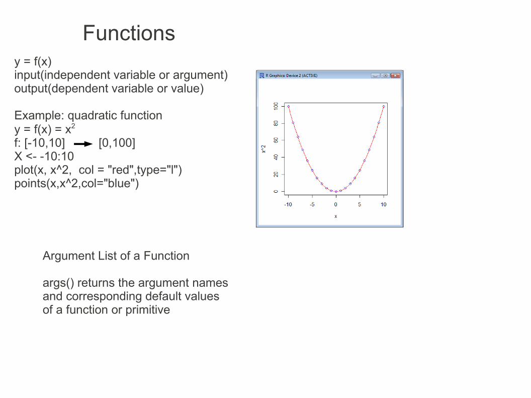
y = f(x)input(independent variable or argument)output(dependent variable or value)
Example: quadratic functiony = f(x) = x2
f: [-10,10] [0,100]X <- -10:10plot(x, x^2, col = "red",type="l")points(x,x^2,col="blue")
Functions
Argument List of a Function
args() returns the argument names and corresponding default values of a function or primitive

Functions
Function Definition
function( arglist ) exprreturn(value)
Argumentsarglist Empty or one or more terms value An expression to be returned
The return command is unnecessary if the function end with the expression tobe returned
A simple function
fncube <- function(x) x^3
fncube(7)fncube(1:5)
function
( arglist )
( value )
Function body(code)
declaration
Function name

Example of using return
Improve the function fncube by returning 0 when the input is a character
fncube <- function(x) x^3
fncube2 <- function(x){if (is.character(x)) return(0) else return(x^3)}
fncube(123)fncube("a")
fncube2(123)fncube2("a")
Functions

Functions
A function with multiple parameters
fnpower <- function(x, n) x^nfnpower(5, 3)fnpower(1:5, 3)fnpower(5, 1:3)fnpower(1:8, 1:2)c(1^1, 2^2, 3^1, 4^2, 5^1, 6^2, 7^1, 8^2)fnpower(1:8, 1:4)c(1^1, 2^2, 3^3, 4^4, 5^1, 6^2, 7^3, 8^4)fnpower(1:8, 1:6) # error!

Functions
A recursive function
Fibonacci sequence, each element is the sum of the previous and the one before
Fibonacci F(n) = Fn-1 + Fn-2, F(0)=0, F(1)=1n=0, 1, 2, ... F(n) = 0, 1, 1, 2, 3, 5, 8, 13, 21
# iterative implementationFibonacci <- function(v){if (v<2) return(v)t <- c(1, 1)for (n in 3:v) t <- c(t, t[n-1]+t[n-2])return(t[v])}
Fibonacci2 <- function(n) ifelse(n==0, 0,ifelse(n==1 | n==2, 1, Fibonacci2(n-1)+Fibonacci2(n-2) ) )
Fibonacci(8)sapply(0:8,Fibonacci)
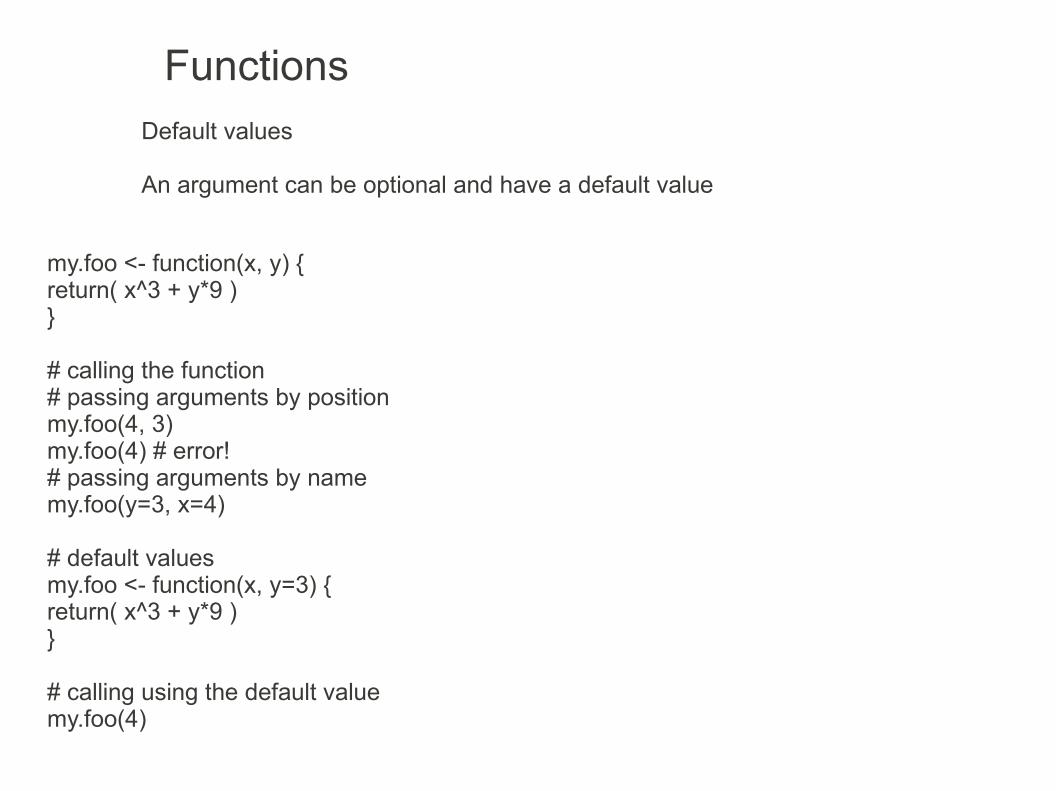
Functions
my.foo <- function(x, y) {return( x^3 + y*9 )}
# calling the function# passing arguments by positionmy.foo(4, 3)my.foo(4) # error!# passing arguments by namemy.foo(y=3, x=4)
# default valuesmy.foo <- function(x, y=3) {return( x^3 + y*9 )}
# calling using the default valuemy.foo(4)
Default values
An argument can be optional and have a default value

Functions
# passing a function as an argumentmy.foo <- function(x, y=3, foo2) {return( foo2(x^3 + y*9) )}
my.foo(2, 3, sin)sin(2^3 + 3*9)
# passing a function as an argument, with parameters for that functionmy.foo <- function(x,y=3, foo2, ...) {return( foo2(x, x^3 + y*9, ...) )}
my.foo(2:20,3, plot,col = "blue",type="l")
Passing functions as arguments
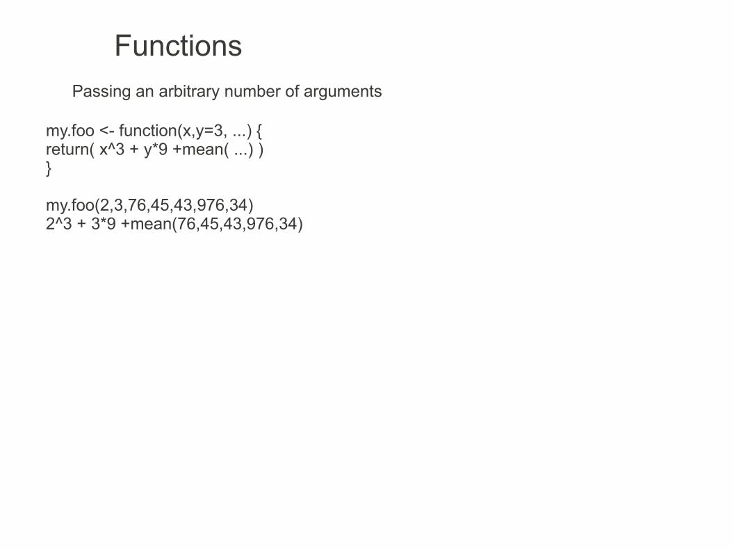
FunctionsPassing an arbitrary number of arguments
my.foo <- function(x,y=3, ...) {return( x^3 + y*9 +mean( ...) )}
my.foo(2,3,76,45,43,976,34)2^3 + 3*9 +mean(76,45,43,976,34)

FunctionsReferences/to learn more:
The R bookMichael J. Crawley pp 472016 John Wiley & Sons Ltd
Statistics: an introduction using RMichael J. Crawley pp 2922014 John Wiley & Sons Ltd
Statistics with RVincent Zoonekynd, pp 27http://zoonek2.free.fr/UNIX/48_R/all.html
Aprendizaje del software estadístico R: un entorno para simulación y computación estadísticaProf. Alberto muñoz garcíaDepartamento de EstadísticaUniversidad Carlos III de Madridhttp://ocw.uc3m.es/estadistica/aprendizaje-del-software-estadistico-r-un-entorno-para-simulacion-y-computacion-estadistica/resolveUid/a70c8973cb8798b0bd0e6bdf7abd6ec7
Introductory Statistics with RPeter Dalgaard, pp 462016 Springer
Software Tools, Part 1: introduction to R softwarePetri Koistinenhttp://www.rni.helsinki.fi/~pek/s-tools/f-own.r
Chem 351 Archives PageDavid Harveyhttp://fs6.depauw.edu:50080/~harvey/Chem%20351/PDF%20Files/Handouts/RDocs/Writing%20Functions%20Using%20R.pdf
Quick-RRob Kabacoffhttp://www.statmethods.net/management/userfunctions.html
The Stem and Tendril simplified R manualProfessors Franzblau, Poje and Verzani of the College of Staten Islandhttp://wiener.math.csi.cuny.edu/st/stRmanual/

The "graphics" package contains many functions for drawing graphics
Graphics on R
high level functions
plotbarplotdotchartstripchartpiehistboxplotpairsstemmosaicplotqqnormcontourperspimage
low level functions(add details to the graphic)
axistitletextlegendpointslinesablinepolygonqqline

Graphics on Rmtcars?mtcars
attach(mtcars)plot(wt, mpg)abline(lm(mpg~wt))title("Regression of MPG on Weight")detach(mtcars)
# instead of attach, "with" would work, not adding to the search pathwith(mtcars, {plot(wt, mpg)abline(lm(mpg~wt))title("Regression of MPG on Weight")})

Graphics on RThe graphic can be saved as an image file from the menu:
Or from code:
win.metafile("MPGonWeight.wmf")postscript("MPGonWeight.ps")pdf("MPGonWeight.pdf")png("MPGonWeight.png")bmp("MPGonWeight.bmp")tiff("MPGonWeight.jpg")jpeg("MPGonWeight.jpg")

Graphics on RPlotting the sine and a parabola:
plot(sin, -pi, 2*pi)plot(function(r) r^2, -pi, 2*pi)
The second plot will overwrite the first one
If that is not the efect wanted:
Multiple graphics
Each graphic on a window
All graphics on separate parts of one window
All graphics merged together, on one window

Graphics on R
Several graphic windows (graphic devices)
To create a graphic device (different commands for different OSs), that will become the active graphic device:windows() or win.graph() WindowsX11() Unixmacintosh() Mac
The first device is device 2, then device 3, etc...
To make a graphic device the active one:dev.set(2) # set active graphic device 2
To close the active graphic devicedev.off()
To close the graphic device 5dev.off(5)

Graphics on Rplot(sin, -pi, 2*pi)windows()plot(function(r) r^2, -pi, 2*pi)
dev.set(2) # set active graphic device 2

Graphics on Rdev.off() # close the active graphic device
dev.off() # close the active graphic device
This graph is gone too
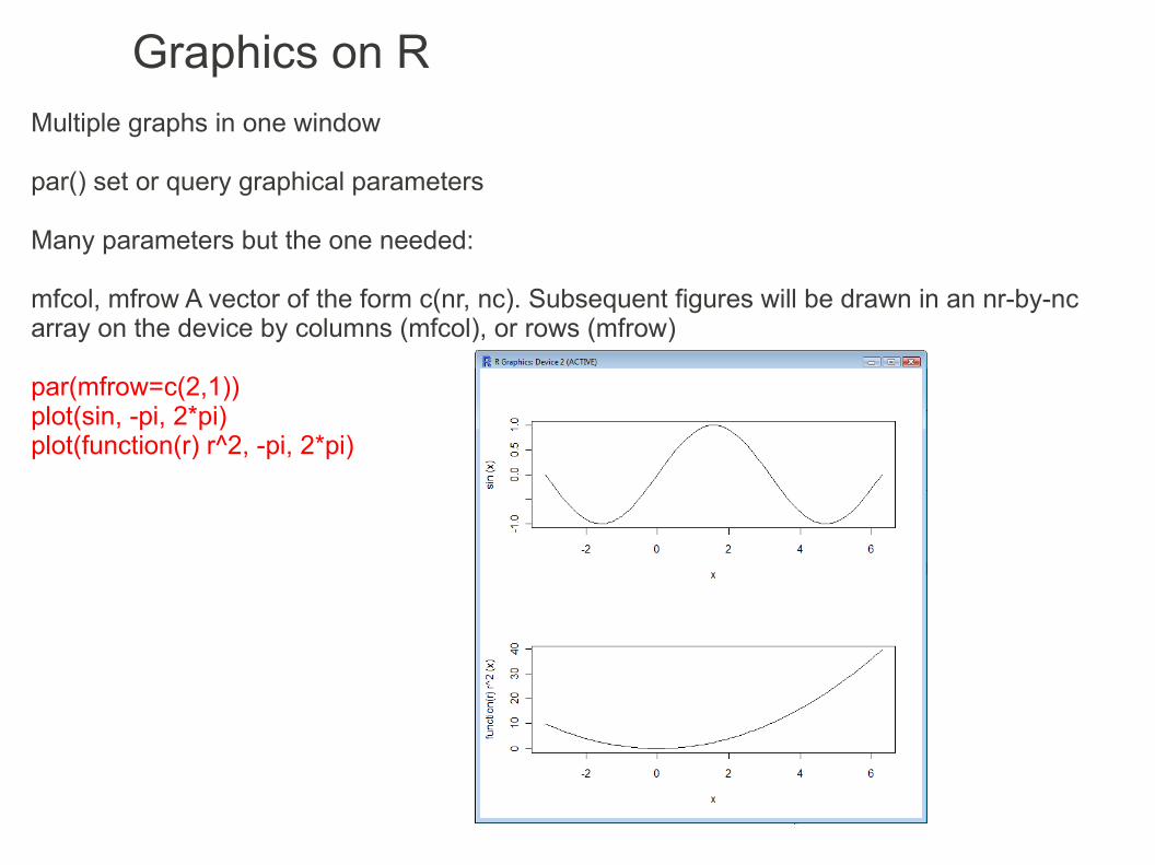
Graphics on RMultiple graphs in one window
par() set or query graphical parameters
Many parameters but the one needed:
mfcol, mfrow A vector of the form c(nr, nc). Subsequent figures will be drawn in an nr-by-nc array on the device by columns (mfcol), or rows (mfrow)
par(mfrow=c(2,1))plot(sin, -pi, 2*pi)plot(function(r) r^2, -pi, 2*pi)

Graphics on Rpar(mfrow=c(1,2))plot(sin, -pi, 2*pi)plot(function(r) r^2, -pi, 2*pi)
par(mfrow=c(2,2))plot(sin, -pi, 2*pi)plot(function(r) r^2, -pi, 2*pi)plot(cos, -pi, 2*pi)plot(function(r) r^3, -pi, 2*pi)

Graphics on R
graphics merged together, on one window
plot(sin, -pi, 2*pi)par(new=T)plot(function(r) r^2, -pi, 2*pi)
The y axis has a different title and scale, making the overlay look funny...
But the two graphs are there!
Graphics on R
Overlaying graphs with different scalesUse different y axis
Use the same scale

Graphics on RUsing different y axis on the same plot
Usually misleading, this seldom used but it is just an example of R's graphing capabilities
par(mar = c(5, 4, 4, 4) + 0.3) # Leave space for z axisplot(sin, -pi, 2*pi)par(new = TRUE)plot(function(r) r^2, -pi, 2*pi, axes = FALSE, bty = "n", xlab = "", ylab = "")axis(side=4, at = pretty( c(pi^2, 4*pi^2) ))mtext("r^2", side=4, line=3)

Graphics on R
plot(sin, -pi, 2*pi, ylim=c(-10,10))par(new=T)plot(function(r) r^2, -pi, 2*pi, ylim=c(-10,10))
plot(sin, -pi, 2*pi, xlim=c(-1,2), ylim=c(-2,2))par(new=T)plot(function(r) r^2, -pi, 2*pi, xlim=c(-1,2), ylim=c(-2,2))
Choosing a range for the x or y axis

Graphics on R
plot()
The plot() function is very versatile and very useful
plot() can draw
simple plotfunction plotline chartscatterplotdensity plot

Graphics on RSimple plot
A simple plot plot(X) has each element of a discrete variable X ploted on the y-axis and the element's index on the x-axis
# simple plotwomenplot(women)
Function plot
A function plot is a simple plot for a continuous variable
# function plotx = seq(-2,2)y = x^2# edgy graph!plot(x,y,type="l",xlab="X axis",ylab="Y axis",main="Parabola", col = "red")# bettersp <- spline(x, y) # spline interpolation of data pointslines(sp, col = "blue")# much bettersp <- spline(x, y,n=20) # interpolation at n points spanning [xmin, xmax]lines(sp, col = "green")

Graphics on RLine chart
A line chart is a simple plot with consecutive plots connected by lines
# line chart
x <- c(1:5); y <- x # create some datapar(pch=22, col="blue") # plotting symbol and colorpar(mfrow=c(2,4)) # all plots on one pageopts = c("p","l","o","b","c","s","S","h")for(i in 1:length(opts)){ heading = paste("type=",opts[i]) plot(x, y, main=heading) lines(x, y, type=opts[i])}
x <- c(1:5); y <- x^4 # create some datapar(pch=22, col="blue") # plotting symbol and colorpar(mfrow=c(2,4)) # all plots on one pageopts = c("p","l","o","b","c","s","S","h")for(i in 1:length(opts)){ heading = paste("type=",opts[i]) plot(x, y, main=heading) lines(x, y, type=opts[i])}

Graphics on R
Scatterplot
A scatterplot plot(X, Y) has each element of a variable Y ploted on the y-axis and the corresponding element for variable X on the x-axis
# scatterplotattach(mtcars)plot(wt, mpg, main="Weight / MPG graph", xlab="Car Weight (lbs)", ylab="Miles Per Gallon", pch=19)
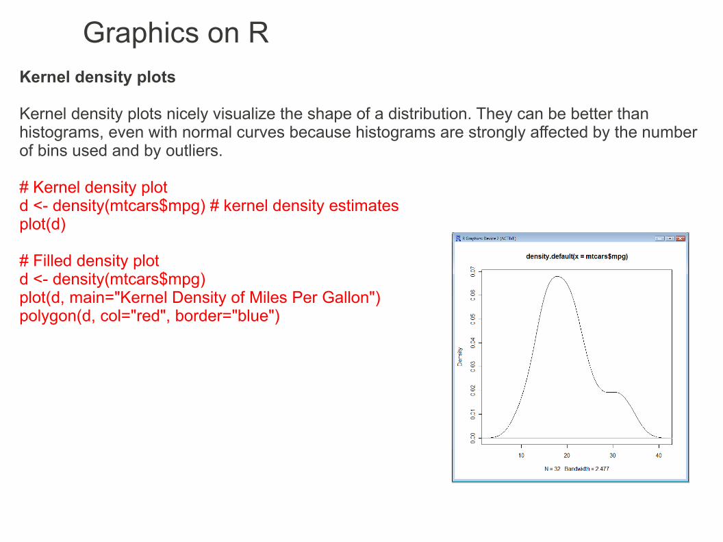
Graphics on RKernel density plots
Kernel density plots nicely visualize the shape of a distribution. They can be better than histograms, even with normal curves because histograms are strongly affected by the number of bins used and by outliers.
# Kernel density plotd <- density(mtcars$mpg) # kernel density estimatesplot(d)
# Filled density plotd <- density(mtcars$mpg)plot(d, main="Kernel Density of Miles Per Gallon")polygon(d, col="red", border="blue")

Graphics on RKernel density for comparing groups
To compare the kernal density plots of two or more groups, the sm package has the function sm.density.compare():sm.density.compare(x, factor)x numeric vectorfactor grouping variable
# Compare MPG distributions for cars with 4,6, or 8 cylinderslibrary(sm)attach(mtcars)
# create value labelscyl.f <- factor(cyl, levels= c(4,6,8), labels = c("4 cylinder", "6 cylinder", "8 cylinder"))
# plot densitiessm.density.compare(mpg, cyl, xlab="Miles Per Gallon")title(main="MPG Distribution by Car Cylinders")
# add legendcolfill<-c(2:(2+length(levels(cyl.f))))legend("topright", levels(cyl.f), fill=colfill)

Graphics on Rbarplot
boxplot(X) is a plot that, if X is a vector, the vector elements are the heights of the bars in the plot, if X is a matrix, the matrix columns are the heights of the bars in the plot, stacked after the first bar (column)If the argument beside=TRUE, then the values in each column are juxtaposed, not stacked. The argument horiz=TRUE creates an horizontal barplot.
VADeathsclass(VADeaths)dimnames(VADeaths)# simple barplotbarplot(VADeaths[,"Rural Male"])# stacked barplotsbarplot(VADeaths[,c("Rural Male", "Rural Female")])# juxtaposed barplotsbarplot(VADeaths[,c("Rural Male", "Rural Female")],beside=T)# stacked barplotsbarplot(VADeaths)# juxtaposed barplotsbarplot(VADeaths,beside=T)

Graphics on Rdotchart
dotchart(X) plots a dot chart or dot plot which plots the values of variable X in groups
# Simple Dotplotdotchart(mtcars$mpg,labels=row.names(mtcars),cex=.7,main="Gas Milage for Car Models",xlab="Miles Per Gallon")
# Dotplot: Grouped Sorted and Colored# Sort by mpg, group and color by cylinderx <- mtcars[order(mtcars$mpg),] # sort by mpgx$cyl <- factor(x$cyl) # it must be a factorx$color[x$cyl==4] <- "red"x$color[x$cyl==6] <- "blue"x$color[x$cyl==8] <- "darkgreen"dotchart(x$mpg,labels=row.names(x),cex=.7,groups= x$cyl,main="Gas Milage for Car Models\ngrouped by cylinder",xlab="Miles Per Gallon",gcolor="black", color=x$color)

stripchart
A stripchart(X) plots a one dimensional or dot plot of the variable X, this is a good alternative to boxplots when sample sizes are small
Data from Cartoon Guide to Statistics, from Larry Gonick, Woollcott Smith, Collins Reference, 1993The weights of some Penn State students, in 1992
mydataf2 <- read.csv("PennState92.csv", header=F,row.names=1)mydataf2# put all the data in one vectorv1 <- c(as.matrix(mydataf2[1,]),as.matrix(mydataf2[2,]))v1 <- v1[!is.na(v1)]# nice strip chartstripchart(v1)# nice strip chart with groupsstripchart(v1, method = "stack",xlim = c(min(v1),max(v1)))

Graphics on Rpie
pie(x) draws a circle (pie) cut into segments (slices), each slice represents a unique value from the elements of x and the sixe of the slice and the relative frequency of each unique value is represented by the size of the slice.
# simple piepie(unique(mtcars$cyl), labels = unique(mtcars$cyl), main="Pie Chart of N. of cylinders")
# pie with percentages and colorswith(mtcars, {n.cyl <- unique(cyl)percent.cyl <-round(table(cyl)/dim(mtcars)[1]*100,2)lbls <- paste(n.cyl," cyl=",percent.cyl,"%", sep="")pie(n.cyl, labels = lbls , main="Pie Chart of N. of cylinders", col=rainbow(length(lbls)))})

Graphics on Rhisthist(X) is an histogram, a bar plot with the frequencies of the values in X on the y-axis and the ranges of values on the x-axisA cumulative distribution curve is the proportion of X on the y-axis, up to the current position on the x-axis
# simple histogramhist(faithful$waiting, prob=TRUE)
# Frequency polygon# http://addictedtor.free.fr/graphiques/RGraphGallery.php?graph=101h <- hist(faithful$waiting, prob=TRUE, plot=FALSE)# compute the frequency polygondiffBreaks <- h$mids[2] - h$mids[1]xx <- c( h$mids[1]-diffBreaks, h$mids, tail(h$mids,1)+diffBreaks )yy <- c(0, h$density, 0)# draw the histogram hist(faithful$waiting, prob = TRUE, xlim=range(xx),border="gray", col="gray90")# adds the frequency polygonlines(xx, yy, lwd=2, col = "royalblue")
# cumulative distributionh <- hist(faithful$waiting)h$counts <- cumsum(h$counts)plot(h)

Graphics on Rboxplot
boxplot(X) is a box-and-whisker plot with the values of variable X, this is an effective way to summarize larger datasets
mydataf2 <- read.csv("PennState92.csv", header=F,row.names=1)mydataf2# plot the data for Males and Femalesapply(mydataf2, 1, summary)boxplot(as.numeric(mydataf2[1,]), as.numeric(mydataf2[2,]), names=c("Males","Females"))

Graphics on R
Changing the scale
mydataf2 <- read.csv("PennState92.csv", header=F,row.names=1)mydataf2
# plot the data for Males and Femalesapply(mydataf2, 1, summary)# use a y-axis scale of 10boxplot(as.numeric(mydataf2[1,]), as.numeric(mydataf2[2,]), names=c("Males","Females"), horizontal=T, xaxt = "n")axis(1, 10:21*10, las = 2)

Graphics on Rmydataf2 <- read.csv("PennState92.csv", header=F,row.names=1)mydataf2
# plot the data for Males and Females# summary points on the y-axisboxplot(as.numeric(mydataf2[1,]), as.numeric(mydataf2[2,]), names=c("Males","Females"), horizontal=T, las = 2)summdtf <- apply(mydataf2, 1, summary)axis(1, summdtf$Males, las = 2, col.axis="red")axis(1, summdtf$Females, las = 2, col.axis="blue")
> apply(mydataf2, 1, summary)$Males Min. 1st Qu. Median Mean 3rd Qu. Max. 123.0 145.0 155.0 158.3 170.0 215.0
$Females Min. 1st Qu. Median Mean 3rd Qu. Max. NA's 95.0 115.5 122.0 123.8 130.5 150.0 22.0
Adding references to points

Graphics on Rboxplot(as.numeric(mydataf2[1,]), as.numeric(mydataf2[2,]), names=c("Males","Females"), horizontal=T, las = 2)summdtf <- apply(mydataf2, 1, summary)axis(1, summdtf$Males, las = 2, col.axis="red")axis(1, summdtf$Females, las = 2, col.axis="blue")
female <- as.numeric(mydataf2[2,])female <- female[!is.na(female)]male <- as.numeric(mydataf2[1,])IQRmale <- IQR(male, na.rm =T) # interquartile rangeIQRfemale <- IQR(female, na.rm =T) # interquartile rangeq1male <- quantile(male,.25, na.rm =T)q3male <- quantile(male,.75, na.rm =T)q1female <- quantile(female,.25, na.rm =T)q3female <- quantile(female,.75, na.rm =T)# whiskers = Q1 - 1.5 * IQR and Q3 + 1.5 * IQRmin(female[female > q1female - 1.5 * IQRfemale])max(female[female < q3female + 1.5 * IQRfemale])min(male[male > q1male - 1.5 * IQRmale])max(male[male < q3male + 1.5 * IQRmale])
axis(1, max(male[male < q3male + 1.5 * IQRmale]), las = 2, col.axis="green")
Calculating the whiskers

Graphics on Rpairs
pairs() shows a matrix with all the scatterplots for the columns of variable X
pairs(~mpg+disp+drat+wt,data=mtcars, main="Scatterplot Matrix MPG, Displacement, Rear axle ratio, Weight")

Graphics on R
stemstem(X) creates a stem-and-leaf plot, which shows the shape of a distribution and displays each observation, useful for small datasets
mydataf2 <- read.csv("PennState92.csv", header=F,row.names=1)mydataf2# put all the data in one vectorv1 <- c(as.matrix(mydataf2[1,]),as.matrix(mydataf2[2,]))v1 <- v1[!is.na(v1)]# stem-and-leaf plotstem(v1)
The decimal point is 1 digit(s) to the right of the |
8 | 5 10 | 288002556688 12 | 000123555550000013555688 14 | 000025555580000000000355555555557 16 | 000045000055 18 | 000500005 20 | 5
Stem Leaf
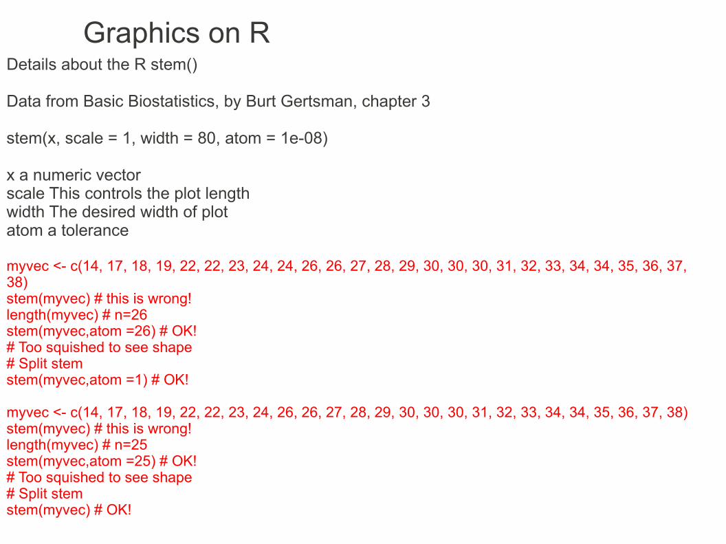
Graphics on RDetails about the R stem()
Data from Basic Biostatistics, by Burt Gertsman, chapter 3
stem(x, scale = 1, width = 80, atom = 1e-08)
x a numeric vectorscale This controls the plot lengthwidth The desired width of plotatom a tolerance
myvec <- c(14, 17, 18, 19, 22, 22, 23, 24, 24, 26, 26, 27, 28, 29, 30, 30, 30, 31, 32, 33, 34, 34, 35, 36, 37, 38)stem(myvec) # this is wrong!length(myvec) # n=26stem(myvec,atom =26) # OK!# Too squished to see shape# Split stemstem(myvec,atom =1) # OK!
myvec <- c(14, 17, 18, 19, 22, 22, 23, 24, 26, 26, 27, 28, 29, 30, 30, 30, 31, 32, 33, 34, 34, 35, 36, 37, 38)stem(myvec) # this is wrong!length(myvec) # n=25stem(myvec,atom =25) # OK!# Too squished to see shape# Split stemstem(myvec) # OK!

Graphics on Rmosaicplot
mosaicplot() draws a mosaic plot, a relationship betwen two or more categorical variables, the widht of the bars is horizontally and vertically proportional to the probabilities associated with the categorical variables
mosaicplot(Titanic, main = "Survival on the Titanic", color = TRUE)## Formula interface for tabulated data:mosaicplot(~ Sex + Age + Survived, data = Titanic, color = TRUE)
## Formula interface for raw data: visualize cross-tabulation of numbers## of gears and carburettors in Motor Trend car data.mosaicplot(~ gear + carb, data = mtcars, color = TRUE, las = 1)# color recyclingmosaicplot(~ gear + carb, data = mtcars, color = 2:3, las = 1)

Graphics on RExamples to explain mosaicplot()
Titanicis(Titanic)dim(Titanic)dimnames(Titanic) # Class Sex Age Survived
# Overall gender proportion the Titanicmosaicplot(~ Sex, main = "Overall gender proportion on the Titanic", data = Titanic, color = TRUE)# ladies firstmosaicplot(~ Sex, main = "Overall gender proportion on the Titanic", data = Titanic[,2:1,,], color = TRUE)
# split vertically by survival ratemosaicplot(~ Sex+ Survived, main = "Overall gender/survival proportion on the Titanic", data = Titanic[,2:1,,], color = TRUE)
#Overall age/survival proportion on the Titanicmosaicplot(~ Age+ Survived, main = "Overall age/survival proportion on the Titanic", data = Titanic, color = TRUE)

Graphics on Rqqnorm and qqline
qqnorm(X) draws a normal probability chart for variable X, with the values of variable X on the y-axis and their associated probability based on a cummulative frequency on the x-axis, assuming a normal distribution
qqline(X) draws the expected linear relationship, assuming a normal distribution
Data from Transcriptomics Bioinformatics, by Attila Gyenesei"An experiment was conducted to evaluate the effectiveness of a treatment for tapeworm in the stomachs of sheep. A random sample of 24 worm-infected lambs of the same age and health was randomly divided into two groups. 12 were injected with the drug and the remaining 12 were left untreated. After a 6-month period the worm counts were recorded"
sheep <- read.table("sheep.txt", sep="\t", header=T)par(mfrow=c(1,2))qqnorm(sheep$treated, main="Treated")qqline(sheep$treated)qqnorm(sheep$untreated, main="Untreated")qqline(sheep$untreated)
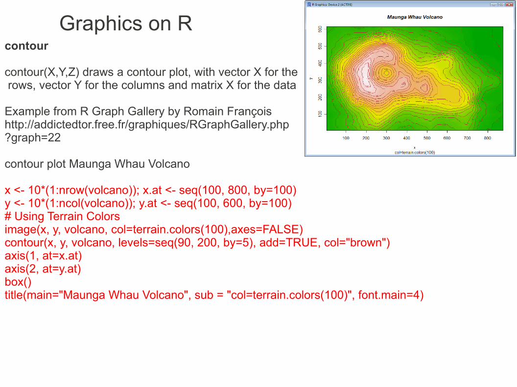
Graphics on Rcontour
contour(X,Y,Z) draws a contour plot, with vector X for the rows, vector Y for the columns and matrix X for the data
Example from R Graph Gallery by Romain François http://addictedtor.free.fr/graphiques/RGraphGallery.php?graph=22
contour plot Maunga Whau Volcano
x <- 10*(1:nrow(volcano)); x.at <- seq(100, 800, by=100) y <- 10*(1:ncol(volcano)); y.at <- seq(100, 600, by=100) # Using Terrain Colorsimage(x, y, volcano, col=terrain.colors(100),axes=FALSE) contour(x, y, volcano, levels=seq(90, 200, by=5), add=TRUE, col="brown") axis(1, at=x.at) axis(2, at=y.at) box() title(main="Maunga Whau Volcano", sub = "col=terrain.colors(100)", font.main=4)

Graphics on Rpersp
persp(X,Y,Z) draws a 3d graph, with vector X for the rows, vector Y for the columns and matrix X for the data
## (2) Visualizing a simple DEM model
z <- 2 * volcano # Exaggerate the reliefx <- 10 * (1:nrow(z)) # 10 meter spacing (S to N)y <- 10 * (1:ncol(z)) # 10 meter spacing (E to W)persp(x, y, z, theta = 120, phi = 15, scale = FALSE, axes = FALSE)

Graphics on RExample from R Graph Gallery by Romain Françoishttp://addictedtor.free.fr/graphiques/RGraphGallery.php?graph=1
Kernel density estimator in R2 Perspective plot and contour plot
require(MASS) set.seed(125)x <- rnorm(150,mean=3*rbinom(150,prob=.5,size=1),sd=1) y <- rnorm(150,mean=4*rbinom(150,prob=.5,size=2),sd=1) d <- kde2d(x,y,n=50) kde2dplot <- function(d, # a 2d density computed by kde2D ncol=50, # the number of colors to use zlim=c(0,max(z)), # limits in z coordinates nlevels=20, # see option nlevels in contour
theta=30, # see option theta in persp phi=30) # see option phi in persp {
z <- d$znrz <- nrow(z) ncz <- ncol(z) couleurs <- tail(topo.colors(trunc(1.4 * ncol)),ncol) fcol <- couleurs[trunc(z/zlim[2]*(ncol-1))+1] dim(fcol) <- c(nrz,ncz) fcol <- fcol[-nrz,-ncz]par(mfrow=c(1,2),mar=c(0.5,0.5,0.5,0.5)) persp(d,col=fcol,zlim=zlim,theta=theta,phi=phi,zlab="density") par(mar=c(2,2,2,2)) image(d,col=couleurs) contour(d,add=T,nlevels=nlevels) box() }kde2dplot(d)

Graphics on R
x <- 1:10 y <- 1:10m <- outer(x,y)mimage(m)
volcanoimage(volcano)
image() Creates a grid of colored or gray-scale rectangles with colors corresponding to the values in z

Graphics on RReferences/to learn more:
The R bookMichael J. Crawley pp 1352017 John Wiley & Sons Ltd
Basic statistics using R pp. 110Jarno Tuimala (CSC) and Dario Greco (HY)http://www.csc.fi/english/csc/courses/archive/R2008s
Statistics: an introduction using RMichael J. Crawley pp 2972015 John Wiley & Sons Ltd
Statistics with RVincent Zoonekynd, pp 147http://zoonek2.free.fr/UNIX/48_R/all.html
Aprendizaje del software estadístico R: un entorno para simulación y computación estadísticaProf. Alberto muñoz garcíaDepartamento de EstadísticaUniversidad Carlos III de Madridhttp://ocw.uc3m.es/estadistica/aprendizaje-del-software-estadistico-r-un-entorno-para-simulacion-y-computacion-estadistica/resolveUid/a68d739b891b9a30368f756ba473b81d
Introductory Statistics with RPeter Dalgaard, pp 712017 Springer
Geographic Data AnalysisPat Bartleinhttp://geography.uoregon.edu/bartlein/courses/geog417/lectures/lec02.htm
Software Tools, Part 1: introduction to R softwarePetri Koistinenhttp://www.rni.helsinki.fi/~pek/s-tools/g-intro.r
Chem 351 Archives PageDavid Harveyhttp://fs6.depauw.edu:50080/~harvey/Chem%20351/PDF%20Files/Handouts/RDocs/Graphing%20Data%20in%20R%20-%20A%20Gallery%20of%20Plots.pdf
Thomas AP Statistics thomasmathematics.comhttp://www.thomasmathematics.com/Aims/Ch1Aim50001.pdf
Quick-RRob Kabacoffhttp://www.statmethods.net/graphs/index.html
The Stem and Tendril simplified R manualProfessors Franzblau, Poje and Verzani of the College of Staten Islandhttp://wiener.math.csi.cuny.edu/st/stRmanual/

Sexual Discrimination at Berkeley
UCBAdmissions(datasets)
This data set is frequently used for illustrating Simpson's paradox, see Bickel et al. (1975). At issue is whether the data show evidence of sex bias in admission practices. There were 2691 male applicants, of whom 1198 (44.5%) were admitted, compared with 1835 female applicants of whom 557 (30.4%) were admitted. This gives a sample odds ratio of 1.83, indicating that males were almost twice as likely to be admitted. In fact, graphical methods (as in the example below) or log-linear modelling show that the apparent association between admission and sex stems from differences in the tendency of males and females to apply to the individual departments (females used to apply more to departments with higher rejection rates).
Simpson's paradoxhttp://en.wikipedia.org/wiki/Simpson%27s_paradox
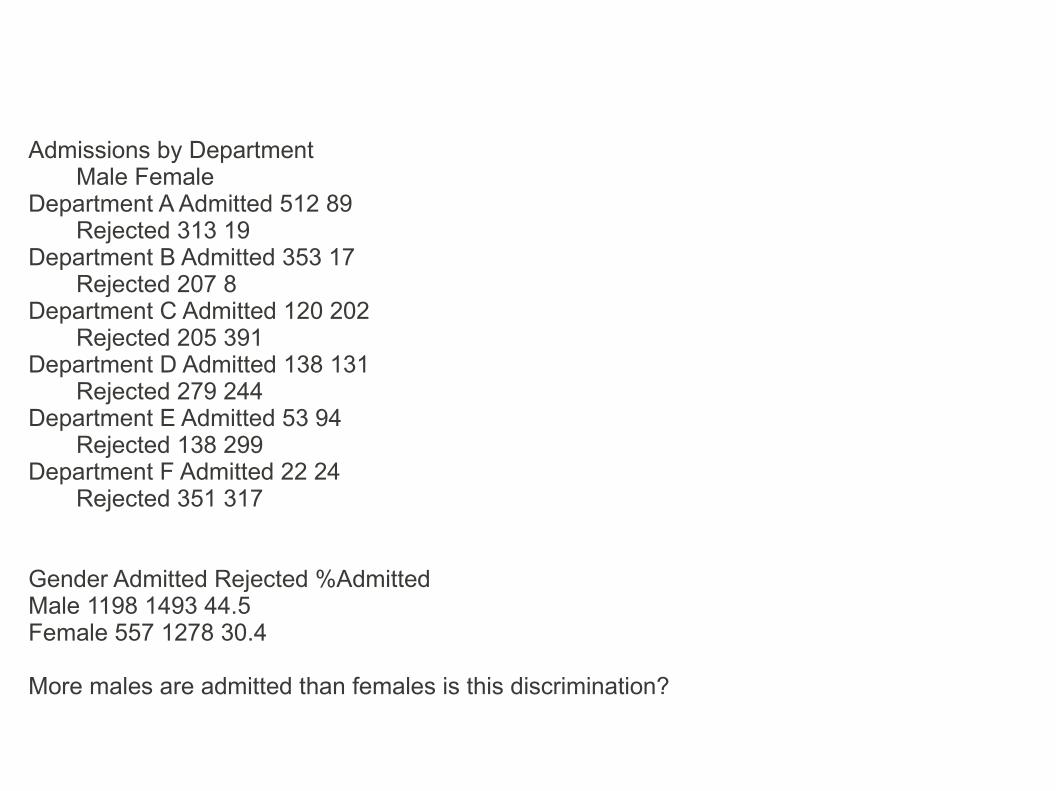
Admissions by DepartmentMale Female
Department A Admitted 512 89Rejected 313 19
Department B Admitted 353 17Rejected 207 8
Department C Admitted 120 202Rejected 205 391
Department D Admitted 138 131Rejected 279 244
Department E Admitted 53 94Rejected 138 299
Department F Admitted 22 24Rejected 351 317
Gender Admitted Rejected %AdmittedMale 1198 1493 44.5Female 557 1278 30.4
More males are admitted than females is this discrimination?

UCBAdmissionsis(UCBAdmissions) # contingency table!dim(UCBAdmissions)rownames(UCBAdmissions)colnames(UCBAdmissions)dimnames(UCBAdmissions)
# creating the table Gender Admitted Rejected %Admitted> apply(UCBAdmissions, 1:2, sum) GenderAdmit Male Female Admitted 1198 557 Rejected 1493 1278> apply(UCBAdmissions, 1:2, sum)[1,]/apply(UCBAdmissions, 2, sum) Male Female 0.4451877 0.3035422
# creating the table Admissions by Department
xtabs(Freq~Dept+Gender+Admit,data=UCBAdmissions)
apply(UCBAdmissions, c(3,2,1), sum)

On a mosaicplot, 2 variables are independent when their proportions are the same, this is not the case
mosaicplot(apply(UCBAdmissions, c(2, 1), sum), main = "Student admissions at UC Berkeley")
More males are admitted!

mosaicplot(UCBAdmissions, sort = 3:1,col = hcl(c(120, 10)),main = "Student admissions at UC Berkeley")
High bias pro Females
low bias pro Males
low bias pro Females
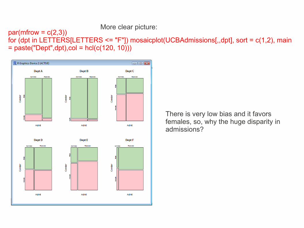
par(mfrow = c(2,3))for (dpt in LETTERS[LETTERS <= "F"]) mosaicplot(UCBAdmissions[,,dpt], sort = c(1,2), main = paste("Dept",dpt),col = hcl(c(120, 10)))
There is very low bias and it favors females, so, why the huge disparity in admissions?
More clear picture:

# which departments admitted less people?mosaicplot(apply(UCBAdmissions, c(3, 1), sum), main = "Student admissions at UC Berkeley")
# which departments did females applied to mostly?mosaicplot(apply(UCBAdmissions, c(3, 2), sum), main = "Student admissions at UC Berkeley")
Females applied mostly to departments that admitted less people, basically competing against each other, while males took the departments more accessible

Saving CSV and TAB from Excel
data from:ECO 231W Econometrics, Summer 07, Session AInstructor: Tak Wai Chauhttp://troi.cc.rochester.edu/~tchau/eco231/height_weight.xls
Height (inches) Weight (lbs) Color of eyes (1=blue, 2=green, 3=brown, 4=other) gender (1=male, 2=female) YearHeight Weight Eyecolor Gender Year
72 190 1 1 200166 130 2 2 200163 98 3 2 2001
72.5 210 1 1 200173 175 4 1 2001
Save as height_weight2.csv

Let's read the table and check out its data:DataStudents<-read.csv("height_weight2.csv",skip=1)DataStudents # Height Weight Eyecolor Gender Year
(a) Calculate the sample means and standard deviations from each variable.mean(DataStudents$Height)mean(DataStudents$Weight)sd(DataStudents$Height)sd(DataStudents$Weight)# ormean(DataStudents[,c("Height","Weight")]) # the mean of height, weightsd(DataStudents[,c("Height","Weight")]) # the sd of height, weight
(b) Calculate the sample means and standard deviations for height and weight, this time by gender.mean(DataStudents[which(DataStudents$Gender==1),c("Height","Weight")]) # the mean of height, weightmean(DataStudents[which(DataStudents$Gender==2),c("Height","Weight")]) # the mean of height, weightsd(DataStudents[which(DataStudents$Gender==1),c("Height","Weight")]) # the sd of height, weightsd(DataStudents[which(DataStudents$Gender==2),c("Height","Weight")]) # the sd of height, weight# oraggregate(DataStudents[,c(1,2,4)], list(DataStudents[,4]), mean)aggregate(DataStudents[,c(1,2,4)], list(DataStudents[,4]), sd)

(c) Calculate the sample means and standard deviations for height and weight, this time by color of eyes.aggregate(DataStudents[,1:3], list(DataStudents[,3]), mean)aggregate(DataStudents[,1:3], list(DataStudents[,3]), sd)
(d) Suppose it is a random sample of students in the university, test the null hypothesis that the mean weight is 200lb for male students against a two-sided alternative.
Null hypothesis H0:μ = 200 Alternative hypothesis H1:μ ≠ 2005% significance levelm=177.9864s=28.42943n= length(which(DataStudents$Gender==1)) = 147T=(177.9864-200)/(28.42943 / sqrt(147))=-9.388184
On R:t.test(DataStudents$Weight[DataStudents$Gender==1], NULL,"two.sided", mu = 200, paired = FALSE, var.equal = FALSE, conf.level = 0.95)
One Sample t-test
data: DataStudents$Weight[DataStudents$Gender == 1] t = -9.3882, df = 146, p-value < 2.2e-16alternative hypothesis: true mean is not equal to 200 95 percent confidence interval: 173.3522 182.6206 sample estimates:mean of x 177.9864
200 is over the confidence interval, in the rejection zone, so it has to be rejected

(e) Suppose it is a random sample of students in the university, test the null hypothesis that mean weights are the same for male and female students.
null hypothesis: mean weights are the same for male and female students
Null hypothesis H0:μ1 = μ2 Alternative hypothesis H1:μ ≠ μ25% significance levelm1=177.9864m2=133.5093s1=28.42943s2=20.10362n1= length(which(DataStudents$Gender==1)) = 147n2= length(which(DataStudents$Gender==2)) = 54T=(177.9864 - 133.5093) / sqrt(28.42943 ^ 2 / 147 + 20.10362 ^ 2 / 54) = 12.34402
On R:t.test(DataStudents$Weight[DataStudents$Gender==1], DataStudents$Weight[DataStudents$Gender==2],"two.sided",paired = FALSE, var.equal = FALSE, conf.level = 0.95)
Welch Two Sample t-test
data: DataStudents$Weight[DataStudents$Gender == 1] and DataStudents$Weight[DataStudents$Gender == 2] t = 12.344, df = 133.349, p-value < 2.2e-16alternative hypothesis: true difference in means is not equal to 0 95 percent confidence interval: 37.35046 51.60382 sample estimates:mean of x mean of y 177.9864 133.5093
Null hypothesis rejected

To do a dot plot in R:dotchart(DataStudents$Weight, main='Students Weight',xlab='Weight in pounds')
stripchart(DataStudents$Weight, method = "stack",xlim = c(min(DataStudents$Weight),max(DataStudents$Weight)))
To examine a distribution of the weight, an histogram is quite useful:
hist(DataStudents$Weight*0.45359237,main='Histogram of weight',xlab='Kilos')

Are men taller and heavier than women?
boxplot(DataStudents$Height ~ DataStudents$Gender, main='Height / Gender', ylab='Height in inches',names=c('Male','Female'))boxplot(DataStudents$Weight ~ DataStudents$Gender, main='Weight / Gender', ylab='Weight in pounds',names=c('Male','Female'))

How are weight and height related? A scatter plot will show all the data.
plot(DataStudents$Height, DataStudents$Weight)

That could be more interesting if the gender was also involved:
sex<-ifelse(DataStudents$Gender==1,'blue','pink')plot(DataStudents$Height, DataStudents$Weight, col=sex)

Who's fat?Using the BMI(Body Mass Index) formula, BMI Overweight >= 25BMI=(weight in pounds * 703 ) / height in inches²So, the curve that separates Overweight people from the rest is:weight = (25 * height in inches²)/703
In R:
sex<-ifelse(DataStudents$Gender==1,'blue','pink')plot(DataStudents$Height, DataStudents$Weight, col=sex)x1<- 50:100 #heighty1<- 25 * x1 * x1 / 703 #weight points(x1, y1,type='l',col='red')
It seems like more men than women are Overweight in this sample data. But there are almost 3 times more men than women and the scatter plot shows one plot for one or more coincident data values and draws the blue over the pink!
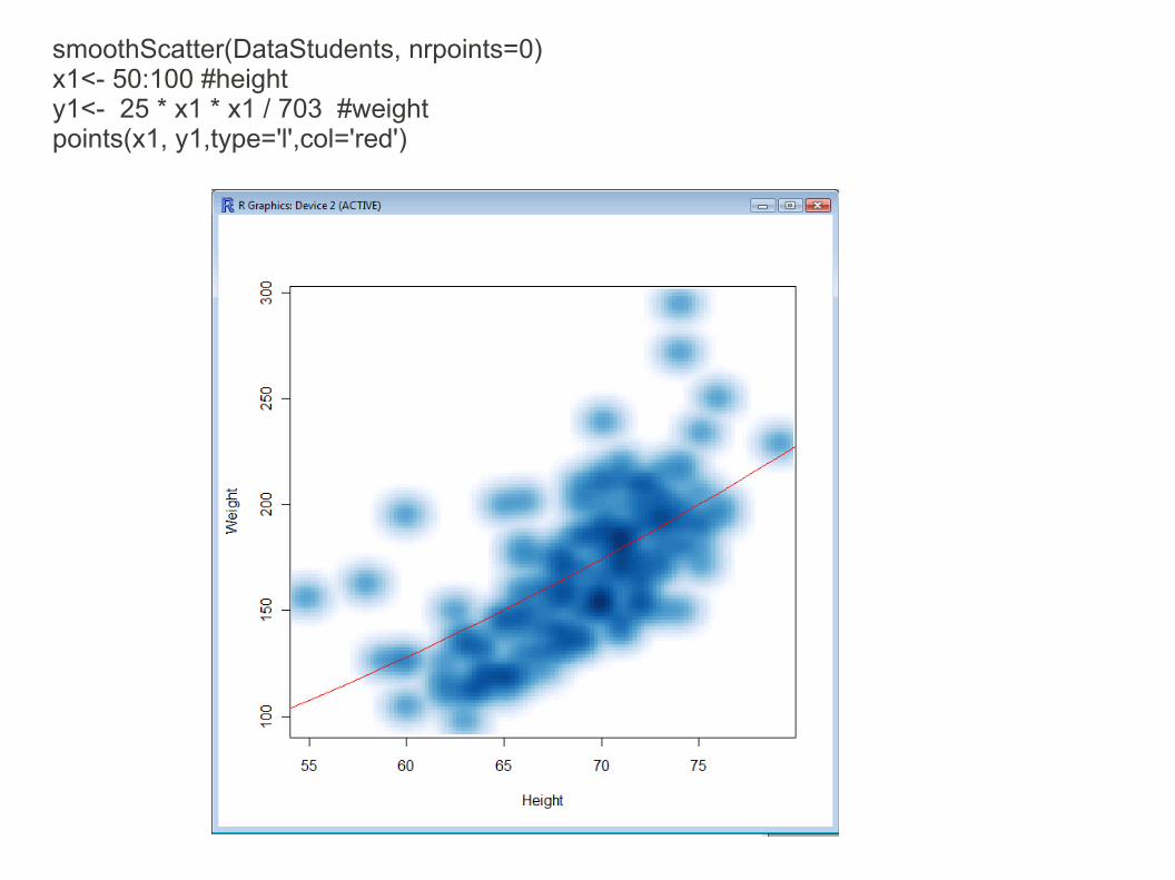
smoothScatter(DataStudents, nrpoints=0)x1<- 50:100 #heighty1<- 25 * x1 * x1 / 703 #weight points(x1, y1,type='l',col='red')

library(RODBC)connection <- odbcConnectExcel("Forbes2000.xls", readOnly = TRUE)#odbcConnectExcel2007connectionsqlTables(connection)
odbcGetInfo(connection)
sqlFetch(connection,'Sheet1$')sqlQuery(connection, "select * from [Sheet1$]")dfForbes2000 <- sqlFetch(connection,'Sheet1$')
class(dfForbes2000)# names of the columnsnames(dfForbes2000)colnames(dfForbes2000)# names of the rows are the row numbers, usually plenty of them!rownames(dfForbes2000)
close(connection)
layout(matrix(1:2, nrow = 2))hist(dfForbes2000$marketvalue)hist(log(dfForbes2000$marketvalue))
Connecting to Excel through ODBC

reactime AUC10 AUC20 AUC30
10 361 729 1105
25 541 1089 1645
55 721 1449 2185
80 901 1809 2725
85 1081 2169 3265
105 1261 2529 3805
110 1441 2889 4345
135 1621 3249 4885
150 1801 3609 5425
155 1981 3969 5965
Problem: the data from a chemical analysis comes in several columns (table 1), each for a different concentration, 10, 20 and 30. AUC is area under the concentration-time curve. The concentration value is stored with the column name, but some statistical analysis would require it to be on a column of its own (table 2)
ReacTime Concentration AUC
10 10 361
10 20 729
10 30 1105
25 10 541
25 20 1089
25 30 1645
55 10 721
55 20 1449
55 30 2185
80 10 901
80 20 1809
80 30 2725
85 10 1081
85 20 2169
85 30 3265
105 10 1261
105 20 2529
105 30 3805
110 10 1441
110 20 2889
110 30 4345
135 10 1621
135 20 3249
135 30 4885
150 10 1801
150 20 3609
150 30 5425
155 10 1981
155 20 3969
155 30 5965
Table 1 Table 2
The data is on a TAB delimited file datawnoise.txt and it will have to be converted and saved onto file datawnoise2.txt

# read table data, TAB separatedRTable<-read.table("datawnoise.txt", header = T, sep = "\t")# examine the dataRTable# store the number of rows and columnsiNrows<-dim(RTable)[1]iNrowsiNcols<-dim(RTable)[2]iNcols# reactime values are needed for each AUC valuerep(RTable$reactime,iNcols-1)# sort the repeated reactime values ReacTime<-sort(rep(RTable$reactime,iNcols-1))ReacTime#get the AUC col namessColName<-colnames(RTable)[-1]sColName# the concentration values are extracted from the AUC column names'sub( "\\D+", "", sColName,perl = TRUE)# concentration values are needed for each original rowConcentration<-rep(sub( "\\D+", "", sColName,perl = TRUE),iNrows)Concentration# convert to vector, by columnsAUC<-c(t(as.matrix(RTable[-1])))#create a matrix with the new datanewdata<-cbind(ReacTime,Concentration,AUC)# save the new datawrite.table(newdata, file = "datawnoise2.txt", sep = "\t",row.names =FALSE, quote =FALSE)

Example from R Graph Gallery by Romain Françoishttp://addictedtor.free.fr/graphiques/RGraphGallery.php?graph=139
Scatterplots with smoothed densities color representation
library("geneplotter") ## from BioConductorrequire("RColorBrewer") ## from CRAN
x1 <- matrix(rnorm(1e4), ncol=2) x2 <- matrix(rnorm(1e4, mean=3, sd=1.5), ncol=2) x <- rbind(x1,x2)
layout(matrix(1:4, ncol=2, byrow=TRUE)) op <- par(mar=rep(2,4)) smoothScatter(x, nrpoints=0) smoothScatter(x) smoothScatter(x, nrpoints=Inf, colramp=colorRampPalette(brewer.pal(9,"YlOrRd")), bandwidth=40) colors <- densCols(x) plot(x, col=colors, pch=20)
par(op)

Open PennState92.xlsSave asPennState92.csv
PennStudents<-read.csv("PennState92.csv",row.names=1,header =F)PennStudents

Statistical Inference
Distributions
standard univariate discrete distributions
binom Binomial Distributionnbinom Binomial negative Distributionpois Poisson Distributiongeom Geometric Distributionhyper Hipergeometric Distribution

Statistical Inference
Distributions
standard univariate continuous distributions
unif Uniform Distributionnorm Normal Distributionlnorm Log-normal Distributionchisq Chi Square Distributiont Student t Distributionf f Distribution Distributionexp Exponential Distributiongamma Gamma Distributionweibull Weibull Distributioncauchy Cauchy Distributionbeta Beta Distributionlogis Logisticsignrank Wilcoxon Signed Rank Statisticwilcox Wilcoxon Rank Sum Statistic

Statistical Inference
Distributions
Multivariate continuous distributions
mvrnormmultivariate normal (pkg MASS)wishWishart (pkg MCMCpack)iwish inverse Wishart (pkg MCMCpack)dirichlet Dirichlet (pkg MCMCpack)mvnorm multivariate normal (pkg mvtnorm)mvt multivariate t (pkg mvtnorm)
Multivariate discrete distributions multinom multinomial

Statistical Inference
Distributions
Functions for distribution "dist"
ddist(x, ... params ..., log=FALSE) density function or probability density function, log=TRUE for log-likelihoods
pdist(q, ... params ..., lower.tail=TRUE, log.p=FALSE) distribution function (cumulative density function), lower.tail=FALSE for one-tailed upper p-values, log.p=TRUE for very small p-values
qdist(p, ... params ...,lower.tail=TRUE,log.p=FALSE) quantile function (inverse cumulative density function)
rdist(n, ... params ...) random deviate generator, n is the number of deviates

Statistical Inference
Distributions
R has several algorithms for pseudo random number generators (RNG), these algorithms will generate the same sequence of pseudo random numbers by specifying the seed for the algorithm (to start the sequence) and the version number (the algorithms are updated for bugs and improvements)
RNG functions
RNGkindRNGversionset.seed
For simplicity, the examples will use the default RNG and change the seed to assure reproducibility of resultsrnorm(5) # draw a sample of size 5 from a normal distributionrnorm(5) # draw a sample of size 5 from a normal distributionrnorm(5) # draw a sample of size 5 from a normal distributionset.seed(2012) # setting a seed for the RNGrnorm(5) # draw a sample of size 5 from a normal distributionrnorm(5) # draw a sample of size 5 from a normal distributionrnorm(5) # draw a sample of size 5 from a normal distributionset.seed(2012) # setting a seed for the RNGrnorm(5) # draw a sample of size 5 from a normal distributionrnorm(5) # draw a sample of size 5 from a normal distributionrnorm(5) # draw a sample of size 5 from a normal distribution
the RNG will return the same sequences for reproducibility of tests

Statistical Inference
Distributions
rnorm(1) # draw a sample of size 1 from a normal distributionrnorm(5) # draw a sample of size 5 from a normal distributionrnorm(5,mean=1,sd=3) # draw a sample of size 5 from a normal distribution with mean 1 and standard deviation 3rnorm(60, 4, 7) # draw a sample of size 60 from a normal distribution with mean 4 and standard deviation 7
dnorm(0) # density for the normal distribution on point 0dnorm(1) # density for the normal distribution on point 1dnorm(3) # density for the normal distribution on point 3pnorm(0) # acumulated probability for the normal distribution below point 0pnorm(3) # acumulated probability for the normal distribution below point 3qnorm(0.5) # quantile 50% of the normal distribution is 0qnorm(0.9986501) # quantile for pnorm(3)x<-seq(-4,4,length=200) # create a sequence of 200 values [-4, 4]plot(x,dnorm(x),type="l") # plot a normal distribution
rpois(50, lambda=3) # draw a sample of size 50 from a Poisson distribution with lambda=3
rbinom(100, 40, .25) # draw a sample of size 100 from a Binomial distribution with size=40 and prob=.25

Statistical Inference
Sampling
sample draws a random sample from a population, replacement=T for sampling with replacement
sample(5) # random permutation of sequence [1, 5]sample(20) # random permutation of sequence [1, 20]
sample(seq(3:45), 10) # random sample of size 10 from [3, 45]
sample(4, 10, prob = c(0.3, 0.5, 0.1, 0.1), replace = T) # random sample of size 10 from sequence [1, 4] with different probabilities of being chosen P(1)=.3, P(2)=.5 etc...
sample(c(0,1), 20, replace = TRUE) # 20 Bernoulli trials
sample(c("heads","tails"),1) # flipping a coin oncesample(c("heads","tails"),5, replace=T) # flipping a coin 5 times
sample(6,1) # rolling a dice oncesample(6,20,replace=T) # rolling a dice 20 times
sample(c("rock","paper", "scisors"),1) # draw rock-paper-scisors once
sample(39, 7) # drawing lottery numbers

Statistical Inference
Tests
One-Sample and Paired Data
t.test t-testwilcox.test Wilcoxon signed rank
Two-Sample t.test t-testwilcox.test Wilcoxon 2-sample rank-sum
k-Samplekruskal.test Kruskal-Wallisoneway.test One-way ANOVA
Unified Unpaired Nonparametric Tests spearman2

Statistical Inference
Tests
# Student's sleep dataplot(extra ~ group, data = sleep)# t testt.test(extra ~ group, data = sleep)

Statistical Inference
Tests
Explanatory
response
continuous categorical
categorical Logistic regression
Cpntigency tables, 2x2, Chi2, Fisher
continuous Regression, correlation
Anova, t-test

Statistical Inference
Correlations
cor( ) correlations
cov( ) covariances
cor.test( ) test a single correlation coefficient
corrgram( ) plot correlograms
# Correlations/covariances among numeric variables in# dataframe mtcars. Use listwise deletion of missing data.cor(mtcars, use="complete.obs", method="kendall")cov(mtcars, use="complete.obs")
# Correlation matrix from mtcars# with mpg, cyl, and disp as rows# and hp, drat, and wt as columnsx <- mtcars[1:3}y <- mtcars[4:6]cor(x, y)

Statistical Inference
Correlations
# First Correlogram Examplelibrary(corrgram)corrgram(mtcars, order=TRUE, lower.panel=panel.shade, upper.panel=panel.pie, text.panel=panel.txt, main="Car Milage Data in PC2/PC1 Order") # Second Correlogram Examplelibrary(corrgram)corrgram(mtcars, order=TRUE, lower.panel=panel.ellipse, upper.panel=panel.pts, text.panel=panel.txt, diag.panel=panel.minmax, main="Car Milage Data in PC2/PC1 Order")
# Third Correlogram Examplelibrary(corrgram)corrgram(mtcars, order=NULL, lower.panel=panel.shade, upper.panel=NULL, text.panel=panel.txt, main="Car Milage Data (unsorted)") http://www.statmethods.net/stats/correlations.html

Statistical Inference
Linear Regression
Model Fitting
Multiple linear regression: lm, ols [Residuals: residuals.ols]General linear model: glm, glmD (just change glm to glmD in call)Binary logistic model: glm, lrmOrdinal logistic model: lrm [Residuals: residuals.lrm]Parametric survival models: survreg, psmCox proportional hazards model: coxph, cph [Residuals: residuals.coxph, residuals.cph]Buckley-James censored least squares regression: bj
After-Fitting Analysis
Specifications for predictor transformations used by Design: specsPredictions and confidence intervals: predict.DesignOverly influential observations: which.influenceSensitivity to unmeasured confounder in lrm: sensucCreate S function to evaluate fitted equation: FunctionCompose LATEX code for typesetting algebraic expressions containing model fit: latex.DesignOdds and hazard ratios and effect differences: summary.DesignGeneral contrasts and CLs: contrast.DesignANOVA: anova.DesignFast backward stepdown variable selection: fastbwHuber-White-Efron robust covariance matrix estimator with optional cluster sampling adjustment: robcovBootstrap nonparametric covariance matrix estimator with optional cluster sampling adjusting: bootcovGenerate data frame with predictor combinations: gendata
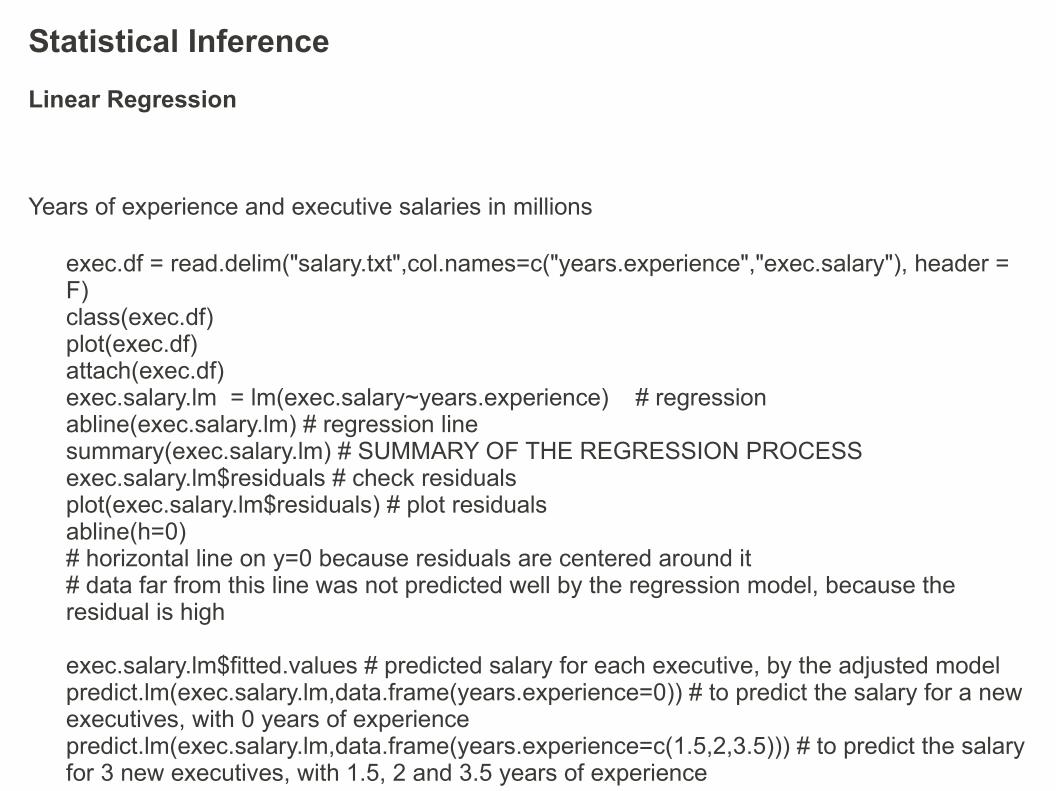
Statistical Inference
Linear Regression
exec.df = read.delim("salary.txt",col.names=c("years.experience","exec.salary"), header = F)class(exec.df)plot(exec.df)attach(exec.df)exec.salary.lm = lm(exec.salary~years.experience) # regressionabline(exec.salary.lm) # regression linesummary(exec.salary.lm) # SUMMARY OF THE REGRESSION PROCESSexec.salary.lm$residuals # check residualsplot(exec.salary.lm$residuals) # plot residualsabline(h=0) # horizontal line on y=0 because residuals are centered around it# data far from this line was not predicted well by the regression model, because the residual is high
exec.salary.lm$fitted.values # predicted salary for each executive, by the adjusted modelpredict.lm(exec.salary.lm,data.frame(years.experience=0)) # to predict the salary for a new executives, with 0 years of experiencepredict.lm(exec.salary.lm,data.frame(years.experience=c(1.5,2,3.5))) # to predict the salary for 3 new executives, with 1.5, 2 and 3.5 years of experience
Years of experience and executive salaries in millions

Statistical Inference
Linear Regression
Simple Linear Regression
0 4.612 6.972 6.362 6.611 3.615 10.150 4.003 8.633 9.340 3.865 12.624 9.423 7.634 9.972 6.330 3.191 5.622 7.984 10.494 8.54

Statistical Inference
Linear Regression
Multiple linear regression
Instead of a regression line there is a regression plane
data(mtcars) # load datasetattach(mtcars)cars.lm = lm(mpg~hp+wt) # explain gas milleage in function of power and weightsummary(cars.lm)# the model is: gas milleage = 37.22 - 0.03 power - 3.87 weight# the more powerful the car, the lower the MPG, less milles per gallon# the heavier the car, the lower the MPG, less milles per gallon# R-Squared is 82%, these 2 variables explain the gas milleage very well
# let's draw the residuals to check if any car behaves differentlyplot(cars.lm$residuals)abline(h=0)
# to predict how many milles per gallon a car with 150 horse power and weight 2.t tons:predict.lm(cars.lm,data.frame(hp=150,wt=2.5))

Statistical Inference
ANOVA
When is Anova Used?• All explanatory variables are categorical—unquantified and unordered• The explanatory variables are called ‘factors’; each has two or more levels.• If there is one factor with two levels, use Student’s t.• If there is one factor with three+ levels, use one-way Anova.• If there are two factors, use two-way Anova.• For three factors, use three-way Anova, and so on…• If every combination of factors is present, you have a factorial design, allowing you to study interactions between variables (and order no longer matters!).

Statistical Inference
ANOVA
Modelling the mileage (mpg) with variables weight (wt), transmission type (am), and/or the number of cylinders (cyl), 3 models:
data(mtcars) # load datasetres.lm = lm(mpg ~ wt, data = mtcars)res.lm2 = lm(mpg ~ wt + cyl, data = mtcars)res.lm3 = lm(mpg ~ wt + cyl + am, data = mtcars)
#Applying anova() to a single model object produces an analysis of variance for computing the F-test ofwhether the constant mean model is appropriateanova(res.lm)
# there is a relationship between mpg and wt
# Applying anova() to two model objects for test if nested models produces an analysis of variance for computing the F-test of whether the extra term is warranted.
anova(res.lm, res.lm2)
# the differences are significant, the number of cylinders seems to have a statistically significant effect.
# Applying anova() to three nested models produces sequential F-tests.anova(res.lm, res.lm2, res.lm3)
# This shows that in the model mpg modeled by wt and cyl, the cyl variable is statistically significant.# However, in the full model of mpg modeled by wt, cyl, and am, the variable am is not statistically significant.# http://wiener.math.csi.cuny.edu/st/stRmanual/anova.pdf

Statistical InferenceReferences/to learn more:
The R bookMichael J. Crawley pp 3702018 John Wiley & Sons Ltd
Basic statistics using R pp. 213Jarno Tuimala (CSC) and Dario Greco (HY)http://www.csc.fi/english/csc/courses/archive/R2008s
Statistics: an introduction using RMichael J. Crawley pp 1252016 John Wiley & Sons Ltd
Statistics with RVincent Zoonekynd, pp 620http://zoonek2.free.fr/UNIX/48_R/all.html
Aprendizaje del software estadístico R: un entorno para simulación y computación estadísticaProf. Alberto muñoz garcíaDepartamento de EstadísticaUniversidad Carlos III de Madridhttp://ocw.uc3m.es/estadistica/aprendizaje-del-software-estadistico-r-un-entorno-para-simulacion-y-computacion-estadistica/resolveUid/4b28fd8154f6521f963aa058ec6baf31
Introductory Statistics with RPeter Dalgaard, pp 1092018 Springer
Geographic Data AnalysisPat Bartleinhttp://geography.uoregon.edu/bartlein/courses/geog417/lectures/lec10.htm
Software Tools, Part 1: introduction to R softwarePetri Koistinenhttp://www.rni.helsinki.fi/~pek/s-tools/test-ci.r
Chem 351 Archives PageDavid Harveyhttp://fs6.depauw.edu:50080/~harvey/Chem%20351/PDF%20Files/Handouts/RDocs/Using%20R%20for%20Linear%20Regression.pdf
Thomas AP Statistics thomasmathematics.comhttp://www.thomasmathematics.com/Aims/Ch3Aim30001.pdf
Quick-RRob Kabacoffhttp://www.statmethods.net/stats/correlations.html
The Stem and Tendril simplified R manualProfessors Franzblau, Poje and Verzani of the College of Staten Islandhttp://wiener.math.csi.cuny.edu/st/stRmanual/

● The rgdal PackageOctober 17, 2008Title for the Geospatial Data Abstraction LibraryVersion .5-27Date -10-09Depends (>= 2.3.0), methods, spLazyLoad Description bindings to Frank Warmerdam’s Geospatial Data Abstraction Library (GDAL) (>= 1.3.1) and access to projection/transformation operations from the PROJ.4 library. TheGDAL and PROJ.4 libraries are external to the package, and, when installing the package fromsource, must be correctly installed first. Both GDAL raster and OGR vector map data can beimported into R, and GDAL raster data and OGR vector data exported. Use is made of classesdefined in the sp package.Author H. Keitt <[email protected]>, Roger Bivand <[email protected]>, Edzer Pebesma <[email protected]>, Barry RowlingsonMaintainer Bivand <[email protected]>License (>= 2)URL ://www.gdal.org, http://rgdal.sourceforge.net/, http://sourceforge.net/projects/rgdal/System Requirements for building from source:GDAL >= 1.3.1 library fromhttp://www.gdal.org/download.html and PROJ.4 (proj >= 4.4.9) from http://proj.maptools.org/
● OGR Simple Feature Library
The OGR Simple Features Library is a C++ open source library (and commandline tools) providing read (and sometimes write) access to a variety of vector file formats including ESRI Shapefiles, S-57, SDTS, PostGIS, Oracle Spatial, and Mapinfo mid/mif and TAB formats.
OGR is a part of the GDAL library.http://www.gdal.org/ogr/

R and GIS
R has several packages that can work with GIS data, the most commonly used is the rgdal Package. The acronym rgdal stands for "R Geospatial Data Abstraction Library".The rgdal Package provides bindings to Frank Warmerdam’s Geospatial Data Abstraction Library (GDAL), this library can work with both raster and vector data in many of the available GIS formats in use. The vector library (OGR) is incorporated into GDAL (raster library) and it is fine to mention either one as separate libraries or GDAL as a whole. RGDAL can work with GDAL raster and OGR vector map files, and it can use both together.
Using rgdal
Loading the library:> library(rgdal)Loading required package: spGeospatial Data Abstraction Library extensions to R successfully loadedLoaded GDAL runtime: GDAL 1.5.3, released 2008/09/09GDAL_DATA: C:/PROGRA~1/R/R-28~1.0/library/rgdal/gdalLoaded PROJ.4 runtime: Rel. 4.6.1, 21 August 2008PROJ_LIB: C:/PROGRA~1/R/R-28~1.0/library/rgdal/proj>
To get a list of the available drivers:> getGDALDriverNames() name long_name create copy1 AAIGrid Arc/Info ASCII Grid FALSE TRUE2 ADRG ARC Digitized Raster Graphics TRUE FALSE3 AIG Arc/Info Binary Grid FALSE FALSE...These are just the first 3, there are over 70, including geoTIFF, ESRI HDR, Erdas IMG, Idrisi RST, USGS DEM, etc...

# To get the gdal version:getGDALVersionInfo()
# Loading dem30m_erdas.img (about 5 Megs):dem30 <- readGDAL('dem30m_erdas.img')
# Getting the projection, datum, etc...proj4string(dem30)
# What kind of variable is dem30?class(dem30)
# Getting detailed information about dem30:summary(dem30)
# dimensions and their namesdim(dem30)names(dem30)
# Plotting a density map:plot(density(dem30$band1))
# read as GDALReadOnlyDatasetdem30 <- GDAL.open('dem30m_erdas.img', read.only = TRUE)# Displaying the rasterdisplayDataset(dem30,offset=c(0,0), region.dim=dim(dem30), reduction=1, band=1)
# Lattice (trellis) plot method for spatial data with attributesspplot(as(dem30, "SpatialGridDataFrame"))

# storing the elevation on a matrixrt <- as.matrix(getRasterTable(dem30)[,3])
# fixing the dimensionsrm<-matrix(rt,dim(dem30)[1],dim(dem30)[2],byrow=T)dim(rt)dim(rm)
# using function image to show the DEMimage(1:dim(dem30)[1],1:dim(dem30)[2],rm)
# using function persp to show the DEMv1 <- seq(1,dim(dem30)[1],100)v2 <- seq(1,dim(dem30)[2],100)persp(1:length(v1), 1:length(v2),rm[v1,v2] )

Cholera mortalities, Soho
Load unit0_slides.R
and read unit0_slides-2x2.pdf
To learn more:
One-day introductory course on Spatial Data Analysis with Rwww.bias-project.org.uk/ASDARcourse
Geographic Data AnalysisGeog 4/517, Pat Bartleinhttp://geography.uoregon.edu/bartlein/courses/geog417/syll09.htm
R for Medicine and BiologyPaul D. Lewis pp 58Jones and Bartlett Series in Biomedical Informatics
Applied Spatial Data Analysis with Rhttp://www.amazon.com/Applied-Spatial-Data-Analysis-Use/dp/0387781706