Embed Size (px)
Citation preview
Review of 2014 Regulatory Financial Statements/2016 Rate Application
E n b r i d g e G a s N e w B r u n s w i c k D e c e m b e r 2 1 2 0 1 5 S c h e d u l e 3 . 9 - G a n n e t t F l e m i n g D e p r e c i a t i o n S t u d y
SCHEDULE 3.9
Gannett Fleming Depreciation Study
ENBRIDGE GAS NEW BRUNSWICK FREDERICTON, NEW BRUNSWICK
2015 DEPRECIATION STUDY
CALCULATED ANNUAL DEPRECIATION ACCRUALS RELATED TO GAS PLANT
AS OF DECEMBER 31, 2014
Prepared by:
Enbridge Gas New Brunswick 2015 Depreciation Study
ENBRIDGE GAS NEW BRUNSWICK Fredericton, New Brunswick
2015 DEPRECIATION STUDY
CALCULATED ANNUAL DEPRECIATION ACCRUALS RELATED TO GAS PLANT
AS OF DECEMBER 31, 2014
GANNETT FLEMING CANADA ULC
Calgary, Alberta
December 21, 2015 Enbridge Gas New Brunswick 440 Wilsey Road Suite101, Fredericton, NB E3B 7G5 Attention: Mr. Paul Volpé Regulatory Affairs Manager Ladies and Gentlemen: Pursuant to your request, we have conducted a review and assessment of the distribution assets of Enbridge Gas New Brunswick. Our report presents a description of the methods used in the estimation of service life and our recommendations for average service life estimates. We gratefully acknowledge the assistance of the Enbridge Gas New Brunswick personnel in the completion of the review.
Respectfully submitted, GANNETT FLEMING CANADA ULC
LARRY E. KENNEDY Vice President LEK/hac Project #060432
Gannett Fleming Canada ULC
Suite 277 • 200 Rivercrest Drive S.E. • Calgary, AB T2C 2X5 • Canada
t: 403.257.5946 • f: 403.257.5947 www.gannettfleming.com
Enbridge Gas New Brunswick 2015 Depreciation Study
TABLE OF CONTENTS
Executive Summary ............................................................................................... v
PART I. INTRODUCTION ...................................................................................... I-1 Scope ...................................................................................................................... I-2 Plan of Report ......................................................................................................... I-2 Basis of the Study ................................................................................................... I-3 Depreciation ................................................................................................ I-3 Service Life Estimates .................................................................................. I-3 PART II. DEVELOPMENT OF DEPRECIATION PARAMETERS ......................... II-1 Depreciation ............................................................................................................ II-2 Estimation of Survivor Curves ................................................................................. II-2
Survivor Curves ............................................................................................ II-2 Survivor Curve Judgments ........................................................................... II-3 PART III. CALCULATION OF ANNUAL AND ACCRUED DEPRECIATION ......... III-1 Calculation of Annual and Accrued Depreciation .................................................... III-2 Group Depreciation Procedures ................................................................... III-2 Calculation of Annual and Accrued Amortization .................................................... III-2 Monitoring of Book Accumulated Depreciation ........................................................ III-4
PART IV. RESULTS OF STUDY ............................................................................ IV-1 Qualification of Results ............................................................................................ IV-2 Description of Detailed Tabulations ......................................................................... IV-2
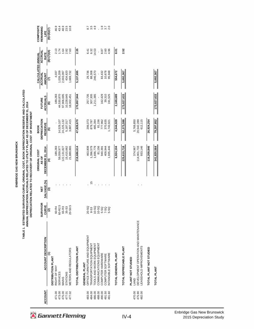
Table 1 Estimated Survivor Curve, Original Cost, Book Depreciation Reserve and Calculated Annual Depreciation Accruals Related To Utility Plant as of December 31, 2014 Depreciation Related to Recovery of Original Cost of Investment ............ IV-4
PART V. SERVICE LIFE STATISTICS .................................................................. V-1 Service Life Statistics .............................................................................................. V-2 PART VII. DETAILED DEPRECIATION CALCULATIONS .................................... VII-1 Detailed Depreciation Calculations ......................................................................... VII-2 APPENDIX A – ESTIMATION OF SURVIVOR CURVES ....................................... A-1 Survivor Curves ....................................................................................................... A-2 Iowa Type Curves ......................................................................................... A-2 Retirement Rate Method of Analysis ............................................................ A-9 Schedules of Annual Transactions in Plant Records .................................... A-9 Schedule of Plant Exposed to Retirements .................................................. A-12 Original Life Table ........................................................................................ A-14 Smoothing the Original Survivor Curve ........................................................ A-16
iv
Enbridge Gas New Brunswick 2015 Depreciation Study
ENBRIDGE GAS NEW BRUNSWICK DEPRECIATION STUDY
EXECUTIVE SUMMARY Pursuant to Enbridge Gas New Brunswick’s (“EGNB” or “Company”) request,
Gannett Fleming Canada ULC (“Gannett Fleming”) conducted a depreciation study
related to distribution plant and general plant accounts as of December 31, 2014. The
purpose of this study was to determine the annual depreciation accrual rates and
amounts for book and ratemaking objectives.
The depreciation rates are based on the straight line method using the average
service life (“ASL”) procedure applied on a remaining life basis. The calculations were
based on attained ages and estimated average service life characteristics for each
depreciable group of assets. Inherent in the use of the remaining life basis, variances
between the calculated accrued depreciation and the book accumulated depreciation as
of December 31, 2014 are amortized over the remaining life of assets.
As EGNB is a utility that is still in an infancy phase, where its ability to grow its
customer connections is vital to its long term viability, the company has not experienced
a significant level of historic retirement activity. Therefore, the recommendations as
contained in this report have relied heavily on the approved average service life
parameters of peer natural gas peer utilities and the broad experience of Gannett
Fleming. Additionally, given the very young age of assets in this company, the
depreciation rate calculations have not included any provision for net negative salvage.
Gannett Fleming recommends the calculated annual depreciation accrual rates
set forth herein apply specifically to distribution plant in service as of December 31,
2014 as summarized by Table 1 of the study by account detail. Supporting data and
calculations are provided as well within the study.
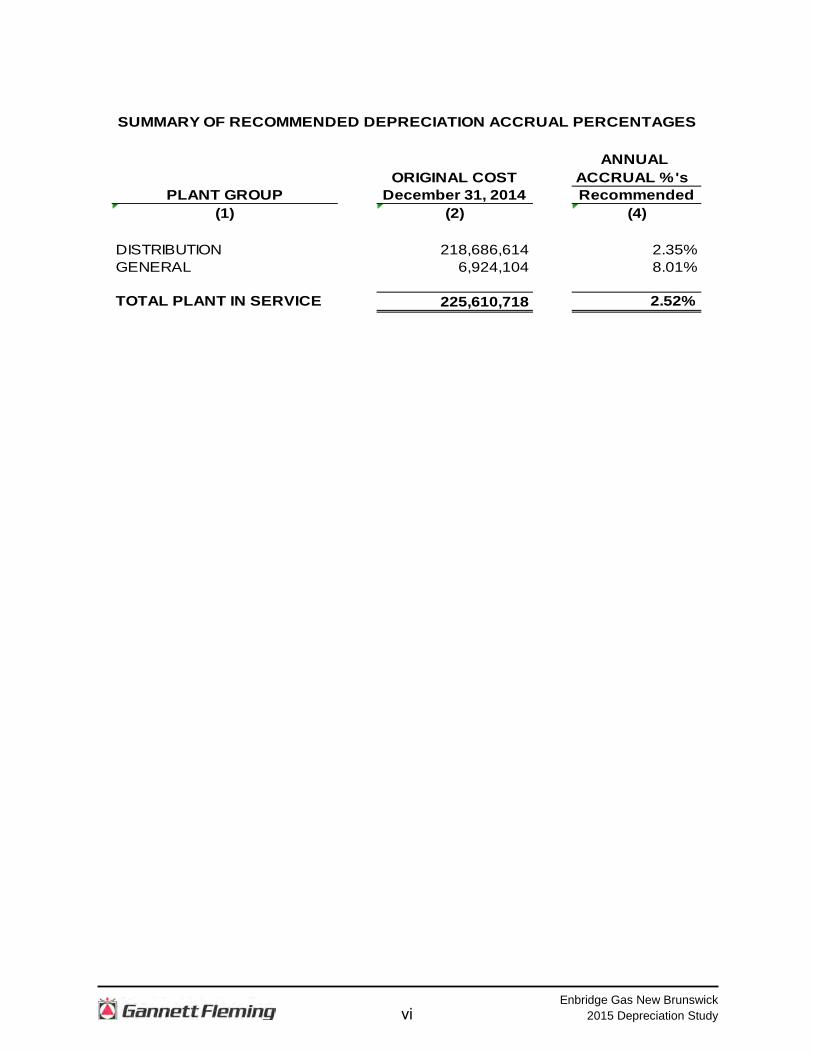
Finally, this study results in a composite depreciation rate for depreciable
property of 2.52%. The report study results are summarized at an aggregate functional
group level as follows:
v
Enbridge Gas New Brunswick 2015 Depreciation Study
ANNUAL ORIGINAL COST ACCRUAL %'s
PLANT GROUP December 31, 2014 Recommended(1) (2) (4)
DISTRIBUTION 218,686,614 2.35%GENERAL 6,924,104 8.01%
TOTAL PLANT IN SERVICE 225,610,718 2.52%
SUMMARY OF RECOMMENDED DEPRECIATION ACCRUAL PERCENTAGES
vi

Enbridge Gas New Brunswick 2015 Depreciation Study
PART I. INTRODUCTION
I-1
Enbridge Gas New Brunswick 2015 Depreciation Study
ENBRIDGE GAS NEW BRUNSWICK DEPRECIATION STUDY
PART I. INTRODUCTION SCOPE
This report sets forth the results of the depreciation study for Enbridge Gas New
Brunswick, to determine the annual depreciation accrual rates and amounts for book
purposes applicable to the original cost of distribution plant at December 31, 2014. The
rates and amounts are based on the straight line remaining life method of depreciation
with a separate amortization of the variance between the book depreciation reserve and
the calculated accrued depreciation. This report also describes the concepts, methods
and judgments which underlie the recommended annual depreciation accrual rates
related to distribution plant in service as of December 31, 2014.
The service life estimates resulting from the study were based on: informed
engineering judgment which incorporated analyses of historical plant retirement data as
recorded through December 31, 2014; a review of Company practice and outlook as
they relate to plant operation and retirement; and consideration of current practice in the
gas industry, including knowledge of service lives used for other gas distribution
companies.
PLAN OF REPORT
Part I Introduction, contains statements with respect to the plan of the report, and
the basis of the study. Part II. Development of Depreciation Parameters, presents
descriptions of the methods used in the service life study. Part III. Calculation of Annual
and Accrued Depreciation presents the methods and procedures used in the calculation
of depreciation. Part IV. Results of Study, presents summaries by depreciable group of
annual and accrued depreciation. Part V presents the results of the Retirement Rate
Analysis and Service Life Statistics Analysis. Detailed tabulations of annual and accrued
depreciation are presented in Part VI of this report. An overview of Iowa curves and the
Retirement Rate Analysis are set forth in Appendix A of the report.
I-2
Enbridge Gas New Brunswick 2015 Depreciation Study
BASIS OF THE STUDY Depreciation
For most accounts, the annual and accrued depreciation were calculated by the
straight line method using the average service life procedure. For certain General Plant
accounts, the annual and accrued depreciation are based on amortization accounting.
Both types of calculations were based on original cost, attained ages, and estimates of
service lives. Variances between the calculated accrued depreciation or amortization
and the book accumulated depreciation are amortized over the composite remaining life
of each account.
Continued monitoring and maintenance of the accumulated depreciation reserve
at the account level is recommended. Gannett Fleming has used the remaining life
basis which will correct the present accumulated depreciation balances to the calculated
accrued depreciation, (“theoretical reserve”), over the composite remaining life of each
account. This adjustment mechanism, whether determined separately as an
amortization amount or incorporated in the calculation of remaining life accruals, is
widely-accepted. An explanation of the monitoring of the accumulated depreciation
reserve and the calculation of the true-up provision is presented beginning on page III-3
of the report.
The straight line method, average service life procedure is a commonly used
depreciation calculation procedure that has been widely accepted in jurisdictions
throughout North America. Gannett Fleming recommends its continued use.
Amortization accounting is used for certain General Plant accounts because of the
disproportionate plant accounting effort required when compared to the minimal original
cost of the large number of items in these accounts. Many gas utilities in North America
have received approval to adopt amortization accounting for these accounts.
Service Life Estimates
The service life estimates used in the depreciation and amortization calculations
were based on informed judgment which incorporated a review of management’s plans,
policies and outlook, a general knowledge of the gas utility industry, and comparisons of
the service life estimates from our studies of other gas utilities. The use of survivor
I-3
Enbridge Gas New Brunswick 2015 Depreciation Study
curves to reflect the expected dispersion of retirement provides a consistent method of
estimating depreciation for gas plant. Iowa type survivor curves were used to depict the
estimated survivor curves for the plant accounts not subject to amortization accounting.
The procedure for estimating service lives consisted of compiling historical data
for the plant accounts or depreciable groups, analyzing this history through the use of
widely accepted techniques, and forecasting the survivor characteristics for each
depreciable group on the basis of interpretations of the historical data analyses and the
probable future. The combination of the historical experience and the estimated future
yielded estimated survivor curves from which the average service lives were derived.
The depreciation rates should be reviewed periodically to reflect the changes that
result from plant and reserve account activity. A depreciation reserve deficiency or
surplus will develop if future capital expenditures vary significantly from those
anticipated in this study.
I-4
Enbridge Gas New Brunswick 2015 Depreciation Study
PART II. DEVELOPMENT OF DEPRECIATIONS PARAMETERS
II-1
Enbridge Gas New Brunswick 2015 Depreciation Study
PART II. DEVELOPMENT OF DEPRECIATION PARAMETERS DEPRECIATION Depreciation, in public utility regulation, is the loss in service value not restored
by current maintenance, incurred in connection with the consumption or prospective
retirement of utility plant in the course of service from causes which are known to be in
current operation and against which the utility is not protected by insurance. Among
causes to be given consideration are wear and tear, deterioration, action of the
elements, inadequacy, obsolescence, changes in the art, changes in demand, and the
requirements of public authorities.
Depreciation, as used in accounting, is a method of distributing fixed capital
costs, less net salvage, over a period of time by allocating annual amounts to expense.
Each annual amount of such depreciation expense is part of that year's total cost of
providing natural gas utility service. Normally, the period of time over which the fixed
capital cost is allocated to the cost of service is equal to the period of time over which
an item renders service, that is, the item's service life. The most prevalent method of
allocation is to distribute an equal amount of cost to each year of service life. This
method is known as the straight-line method of depreciation.
The calculation of annual and accrued depreciation based on the straight line
method requires the estimation of survivor curves and is described in the following
sections of this report. The development of the proposed depreciation rates also
requires the selection of group depreciation procedures, as discussed in Part III of this
report.
ESTIMATION OF SURVIVOR CURVES Survivor Curves The use of an average service life for a property group implies that the various
units in the group have different lives. Thus, the average life may be obtained by
determining the separate lives of each of the units, or by constructing a survivor curve
by plotting the number of units which survive at successive ages using the retirement
rate method of analysis.
II-2
Enbridge Gas New Brunswick 2015 Depreciation Study
The range of survivor characteristics usually experienced by utility and industrial
properties is encompassed by a system of generalized survivor curves known as the
Iowa type curves. There are four families in the Iowa system, labeled in accordance with
the location of the modes of the retirements in relationship to the average life and
relative height of the modes. The left-moded curves are those in which the greatest
frequency of retirement occurs to the left of, or prior to, average service life. The
symmetrical-moded curves are those in which the greatest frequency of retirement
occurs at average service life. The right-moded curves are those in which the greatest
frequency occurs to the right of, or after, the average service life. The origin-moded
curves are those in which the greatest frequency of retirement occurs at the origin, or
immediately after age 0. The letter designation of each family of curves (L, S, R or O)
represents the mode of the associated frequency curve with respect to the average
service life. The numerical subscripts represent the relative heights of the modes of the
frequency curves within each family.
A discussion of the general concept of survivor curves and retirement rate
method is presented in Appendix A of this report.
Survivor Curve Judgments The survivor curve estimates were based on judgment which considered a
number of factors. The primary factors were the professional judgment of Gannett
Fleming, supported by the statistical analysis of data; current policies and outlook as
determined during conversations with management personnel and on the knowledge
Gannett Fleming developed through the completion of numerous gas utility studies.
The following discussion, dealing with a number of accounts which comprise the
majority of the investment analyzed, presents an overview of the factors considered by
Gannett Fleming in the determination of the average service life estimates. The survivor
curve estimates for the remainder of the accounts not discussed in the following
sections were based on similar considerations.
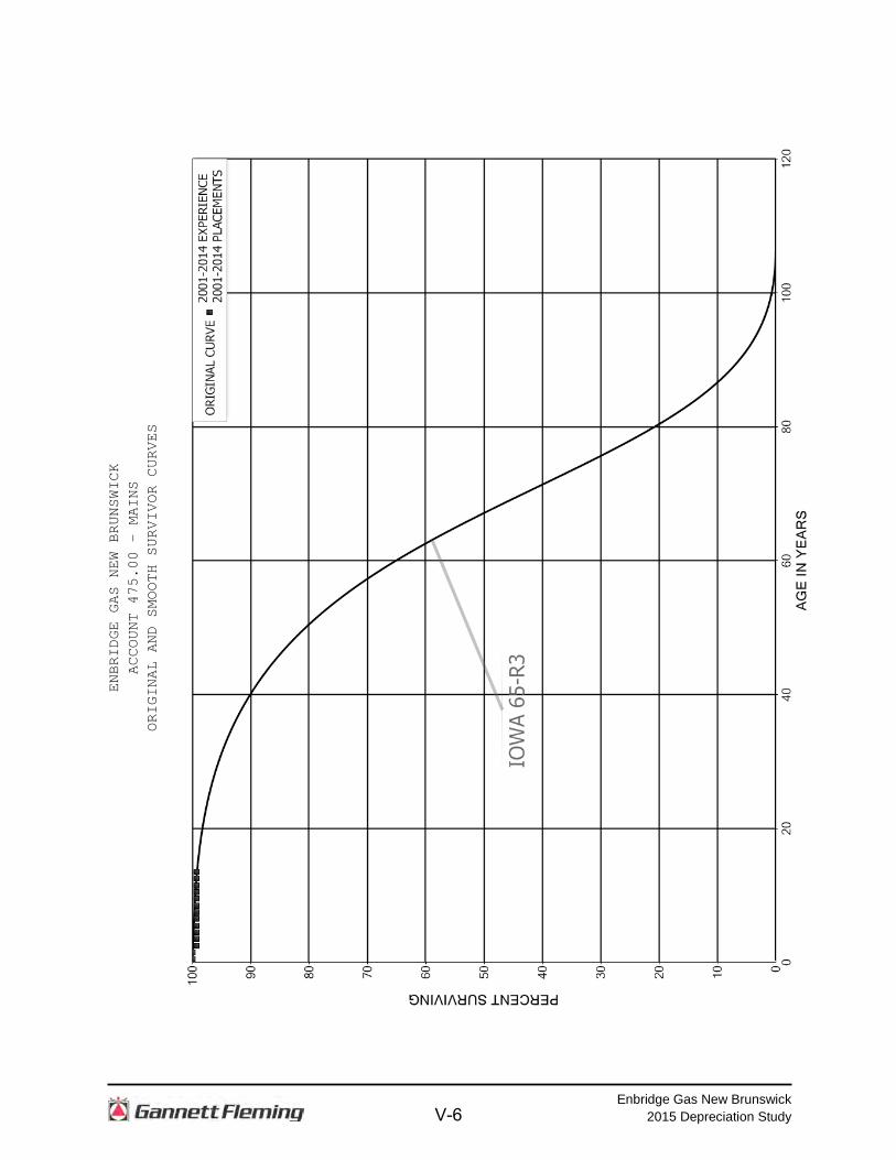
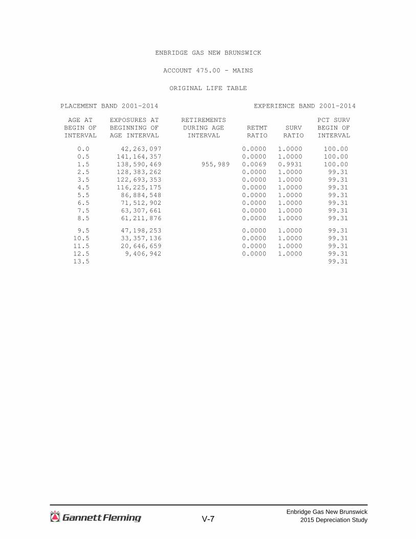
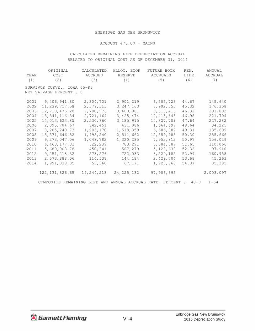
Account 475.00 – Mains, is the largest account studied and represents 54% of
EGNB’s depreciable plant. The retirements, additions and other plant transactions for
the period 2001 through 2014 were analyzed by the retirement rate method. The
II-3
Enbridge Gas New Brunswick 2015 Depreciation Study
original and smooth survivor curve is plotted on page V-6. Typical service lives for
distribution mains range from 55 to 80 years. EGNB’s mains system is comprised of
82% plastic lines versus a small percentage (18%) steel lines.
To date, this account has experienced nearly $1 million of retirement activity.
Discussions with operating and engineering staff have not indicated any specific
reasons to believe that the future retirement trends in this account will be significantly
different than the historic indications. Furthermore, operations staff has indicated that it
would be expected that the life of the EGNB distribution mains would be in the range of
other industry peers and with the EGNB Transmission mains.
Gannett Fleming has recommended an Iowa 65-R3 survivor curve to better
reflect the conservative range of the peer comparators given the relative age of the
assets in his account.
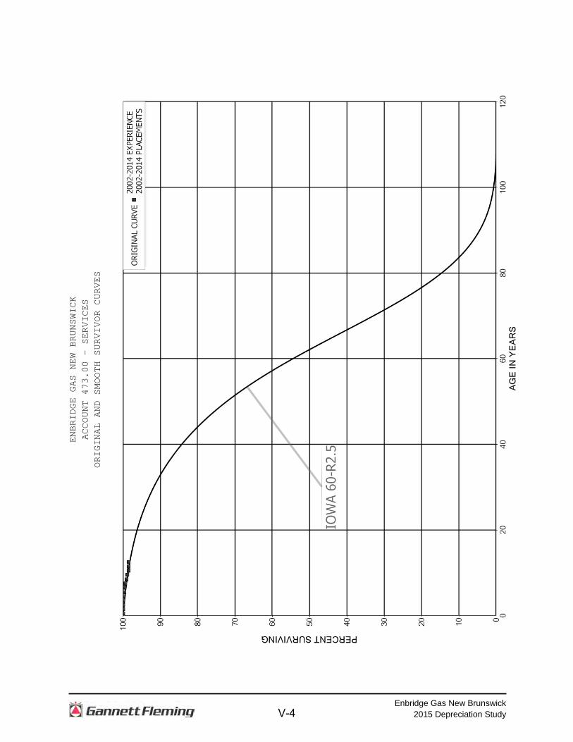
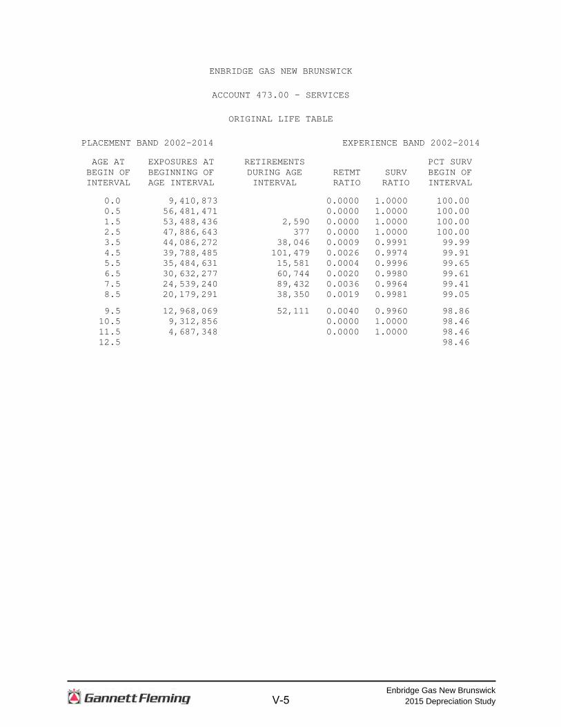
Account 473.00 – Services, represents 26% of EGNB’s depreciable plant. The
retirements, additions and other plant transactions for the period 2002 through 2014
were analyzed by the retirement rate method. The original and smooth survivor curves
are plotted on page V-4.
To date, this account has experienced under $0.4 million of retirement activity.
Discussions with operating and engineering staff indicated that it would be expected
that the life of the EGNB distribution services would be in the range of other industry
peers. Typical service lives for peer Canadian distribution services range from 48 to 62
years.
Based on Gannett Fleming’s experience and the lives of peer gas utilities,
Gannett Fleming recommends the Iowa 60-R2.5 to represent future retirement patterns.
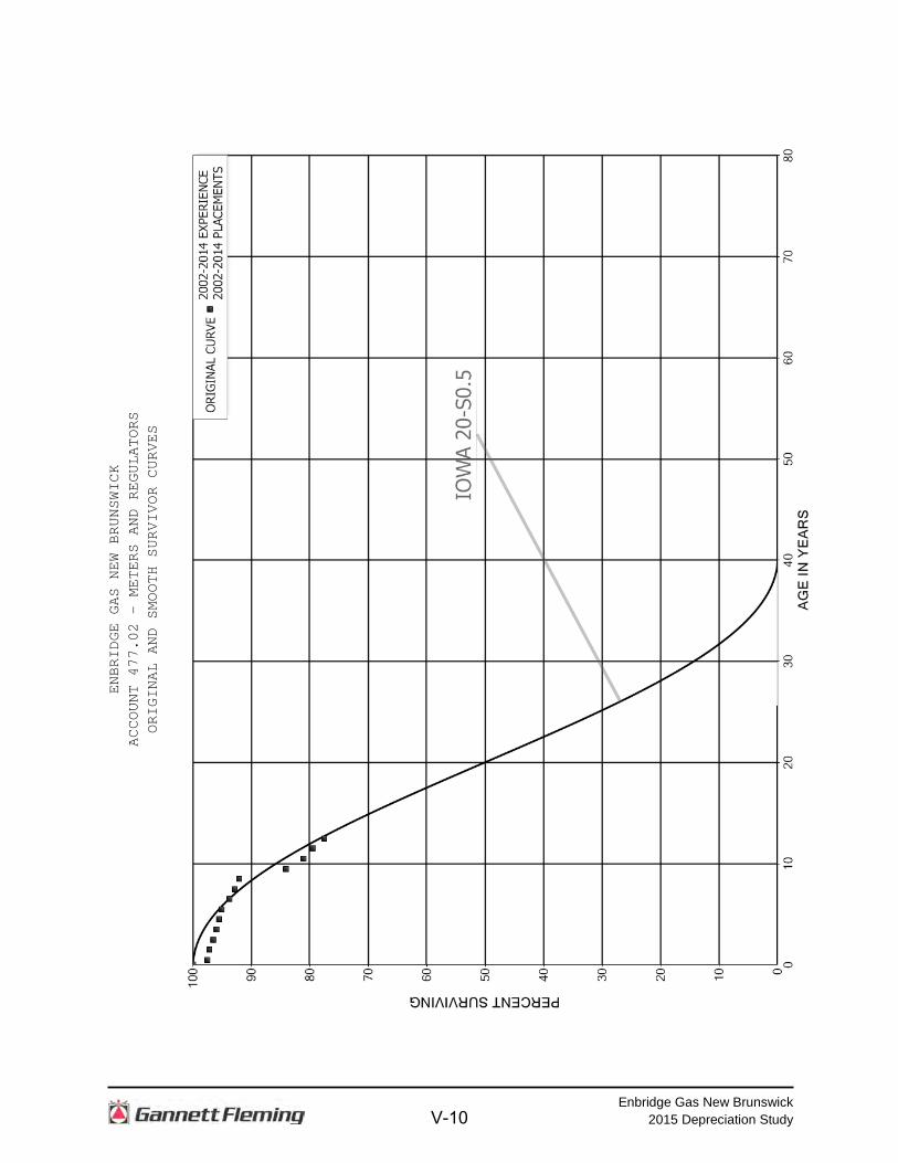
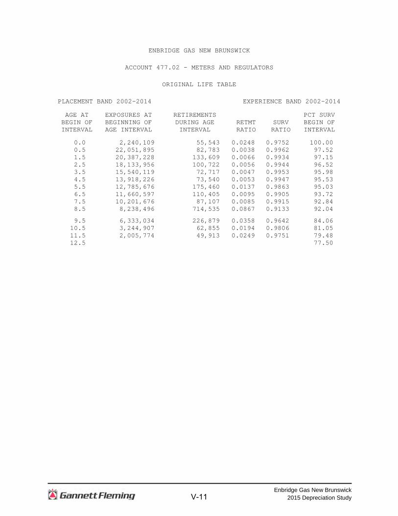
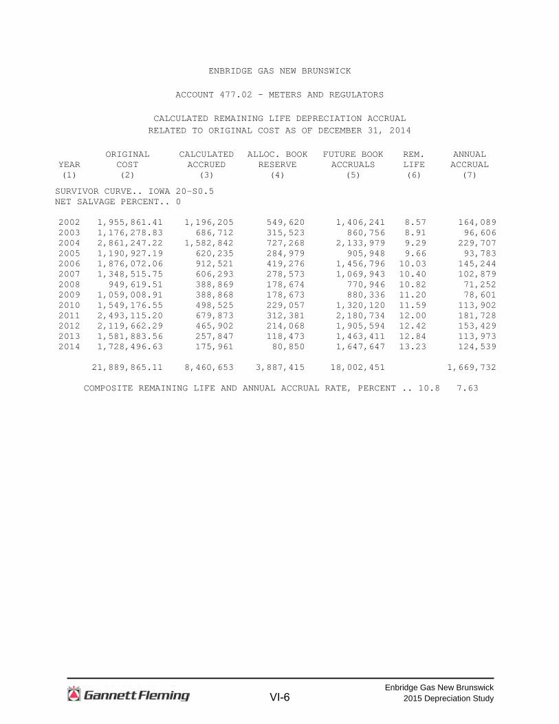
Account 477.02 – Meters and Regulators, represents 10% of EGNB’s
depreciable plant. The retirements, additions and other plant transactions for the period
2002 through 2014 were analyzed by the retirement rate method. The original and
smooth survivor curves are plotted on page V-10. Typical service lives for gas
distribution meters range from 12 to 45 years. To date, this account has experienced
nearly $1.9 million of retirement activity.
In recent years, the gas distribution industry has been moving toward increased
used of digital metering and Automated Meter Reading (AMR) technology. Additionally,
II-4
Enbridge Gas New Brunswick 2015 Depreciation Study
in early 2010, Measurement Canada has announced more stringent metering testing
guidelines. The new testing guidelines place increasingly strict criteria on the test results
as the age of the meters increase.
Interviews with the operational metering staff have indicated that the
implementation of the new Measurement Canada requirements will result in residential
meters being retired before they reach 20 years of age. In the experience of Gannett
Fleming, this assumption is consistent with the metering experts across Canada, all of
whom have indicated that residential meters will no longer be tested when they reach
15 to 20 years of age. Operations staff did indicate that the meters related to
commercial and industrial customers are expected to last beyond 20 years, and would
likely be refurbished when removed for testing.
Gannett Fleming recommends an Iowa 20-S0.5 curve to represent the retirement
characteristics for this account. This account is experiencing significant change in the
technology associated with the assets within this account. Therefore, given the future
expectation that residential meters will be retired prior to reaching an age of 20 years,
this account will be closely monitored over the next few years to determine if a further
shortening of the average service life estimate becomes necessary.
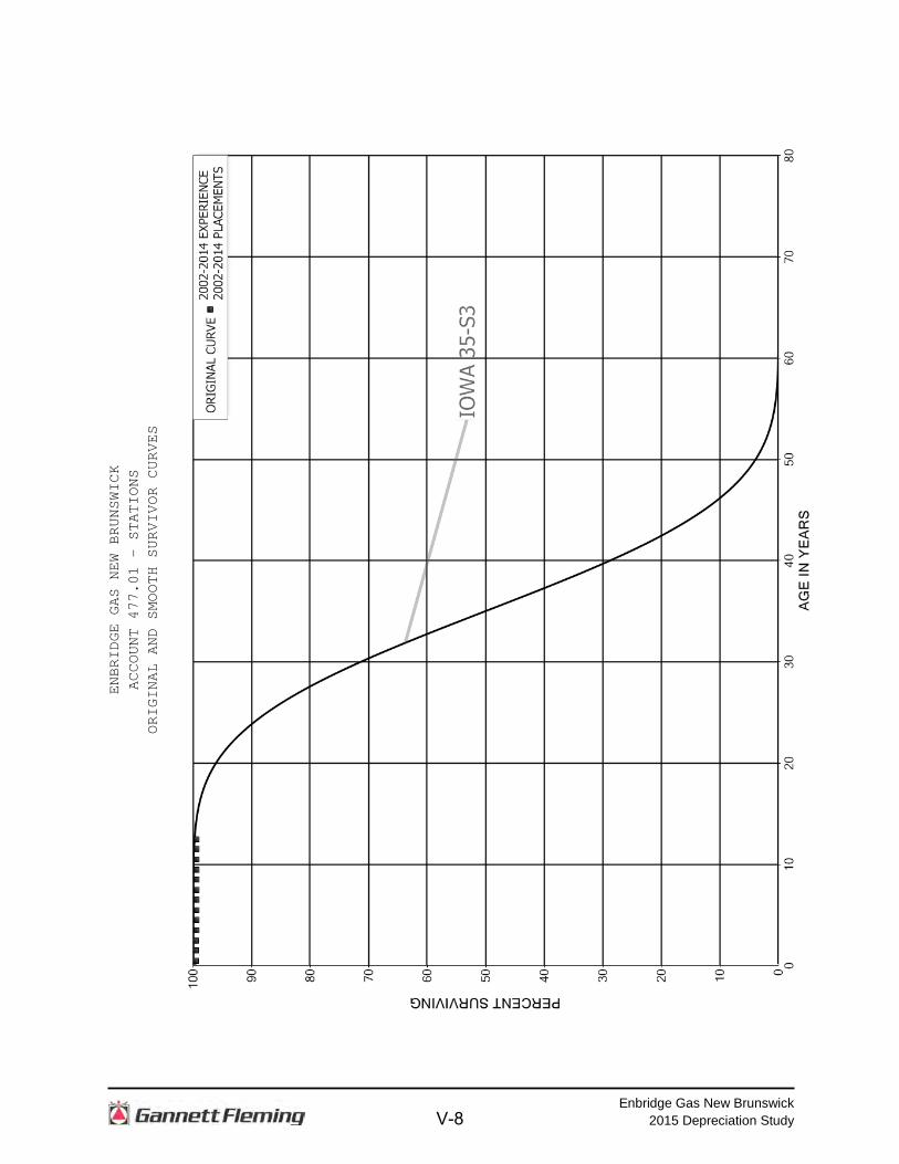
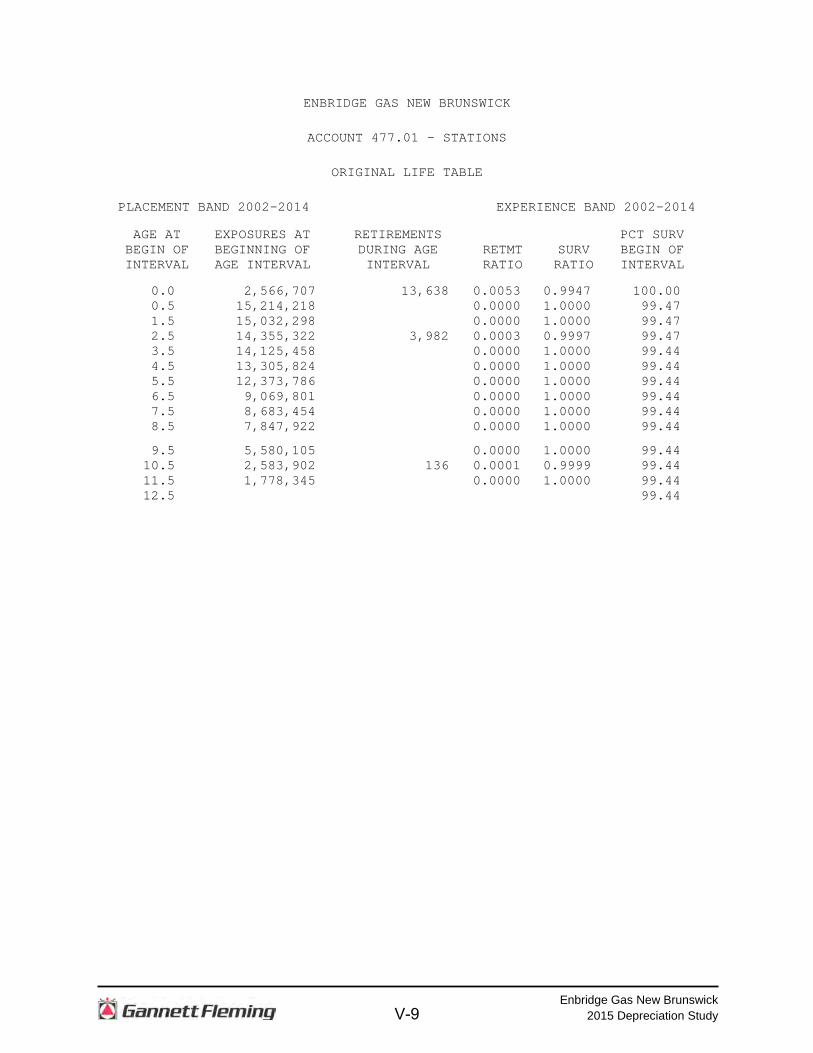
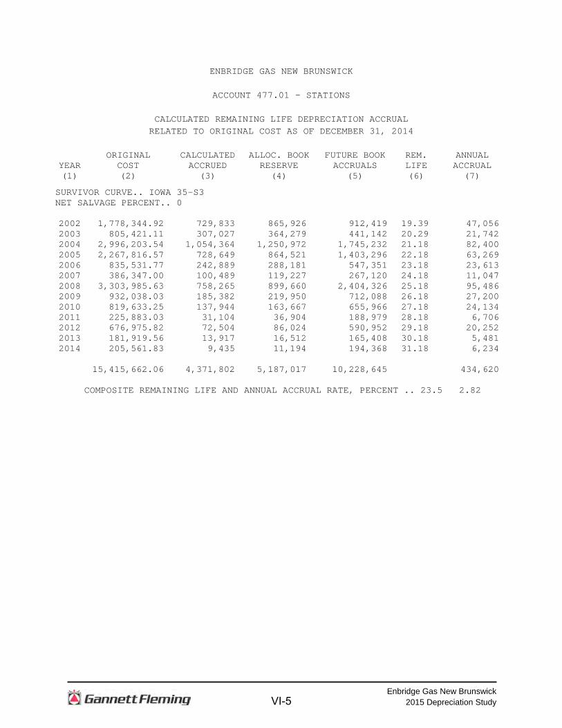
Account 477.01 – Stations, represents approximately 7% of the depreciable plant
studied. The retirements, additions and other plant transactions for the period 2002
through 2014 were analyzed by the retirement rate method. The original survivor curve
as plotted on page V-8 indicates only a small level of historical retirements through age
12, relatively insignificant compared to the total exposures of $123 million indicating a
reliance on peer comparators and professional expertise. Gannett Fleming recommends
a 35-S3 Iowa curve based on industry peers and the discussions with operating and
engineering staff have not indicated any specific reason to believe it would deviate from
the recommended Iowa curve.
The survivor curves estimates for the remaining accounts were based on similar
considerations of historical analysis, management outlook and estimates of this
company and other gas distribution companies.
II-5
Enbridge Gas New Brunswick 2015 Depreciation Study
PART III. CALCULATION OF ANNUAL AND ACCRUED DEPRECIATION
III-1
Enbridge Gas New Brunswick 2015 Depreciation Study
PART III. CALCULATION OF ANNUAL AND ACCRUED DEPRECIATION CALCULATION OF ANNUAL AND ACCRUED DEPRECIATION Group Depreciation Procedures When more than a single item of property is under consideration, a group
procedure for depreciation is appropriate because normally all of the items within a
group do not have identical service lives, but have lives that are dispersed over a range
of time. There are two primary group procedures, namely, Average Service Life (ASL)
and Equal Life Group (ELG).
In the average service life procedure, the rate of annual depreciation is based on
the average service life of the group, and this rate is applied to the surviving balances of
the group's cost. A characteristic of this procedure is that the cost of plant retired prior to
average life is not fully recouped at the time of retirement, whereas the cost of plant
retired subsequent to the average life is more than fully recouped. Over the entire life
cycle, the portion of cost not recouped prior to average life is balanced by the cost
recouped subsequent to average life.
In the equal life group procedure, also known as the unit summation procedure,
the property group is subdivided according to service life. That is, each equal life group
includes that portion of the property which experiences the life of that specific group.
The relative size of each equal life group is determined from the property's life
dispersion curve. The calculated depreciation for the property group is the summation of
the calculated depreciation based on the service life of each equal life unit.
In the determination of the depreciation rates in this study, the use of the average
service life procedure has been used. While the equal life group procedure provides an
enhanced matching of depreciation expense to the consumption of service value, the
average service life procedure.
CALCULATION OF ANNUAL AND ACCRUED AMORTIZATION Amortization is the gradual extinguishment of an amount in an account by
distributing such amount over a fixed period, over the life of the asset or liability to which
it applies, or over the period during which it is anticipated the benefit will be realized.
III-2
Enbridge Gas New Brunswick 2015 Depreciation Study
Normally, the distribution of the amount is in equal amounts to each year of the
amortization period.
The calculation of annual and accrued amortization requires the selection of an
amortization period. The amortization periods used in this report were based on
judgment which incorporated a consideration of the period during which the assets will
render most of their service, the amortization period and service lives used by other
utilities, and the service life estimates previously used for the asset under depreciation
accounting.
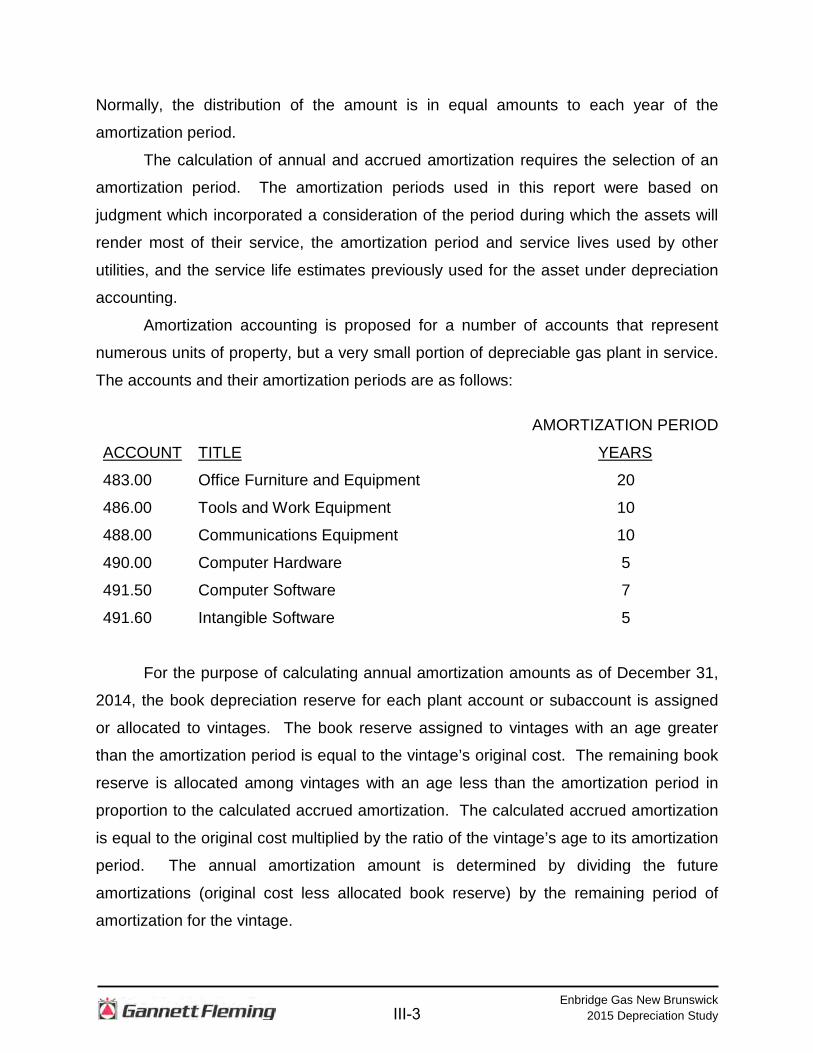
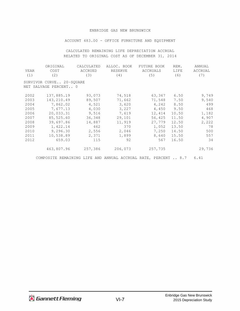
Amortization accounting is proposed for a number of accounts that represent
numerous units of property, but a very small portion of depreciable gas plant in service.
The accounts and their amortization periods are as follows:
AMORTIZATION PERIOD
ACCOUNT TITLE YEARS
483.00 Office Furniture and Equipment 20
486.00 Tools and Work Equipment 10
488.00 Communications Equipment 10
490.00 Computer Hardware 5
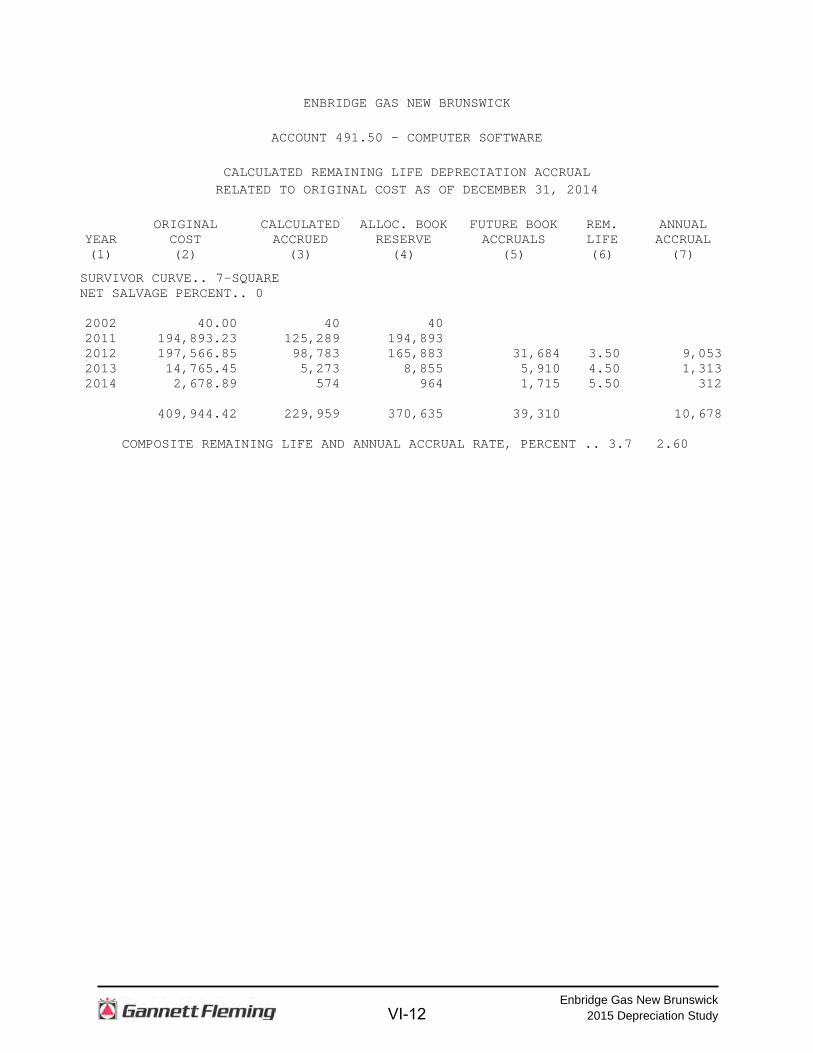
491.50 Computer Software 7
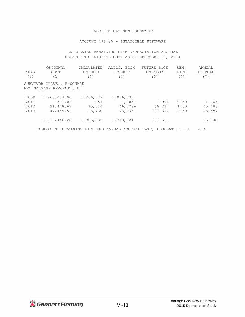
491.60 Intangible Software 5
For the purpose of calculating annual amortization amounts as of December 31,
2014, the book depreciation reserve for each plant account or subaccount is assigned
or allocated to vintages. The book reserve assigned to vintages with an age greater
than the amortization period is equal to the vintage’s original cost. The remaining book
reserve is allocated among vintages with an age less than the amortization period in
proportion to the calculated accrued amortization. The calculated accrued amortization
is equal to the original cost multiplied by the ratio of the vintage’s age to its amortization
period. The annual amortization amount is determined by dividing the future
amortizations (original cost less allocated book reserve) by the remaining period of
amortization for the vintage.
III-3
Enbridge Gas New Brunswick 2015 Depreciation Study
MONITORING OF BOOK ACCUMULATED DEPRECIATION The calculated accrued depreciation or amortization represents that portion of
the depreciable cost which will not be allocated to expense through future depreciation
accruals, if current forecasts of service life characteristics materialize and are used as a
basis for depreciation accounting. Thus, the calculated accrued depreciation provides a
measure of the book accumulated depreciation. The use of this measure is
recommended in the amortization of book accumulated depreciation variances to insure
complete recovery of capital over the life of the property.
The recommended amortization of the variance between the book accumulated
depreciation and the calculated accrued depreciation is based on an amortization period
equal to the composite remaining life for each property group where the variance
exceeds five percent of the calculated accrued depreciation.
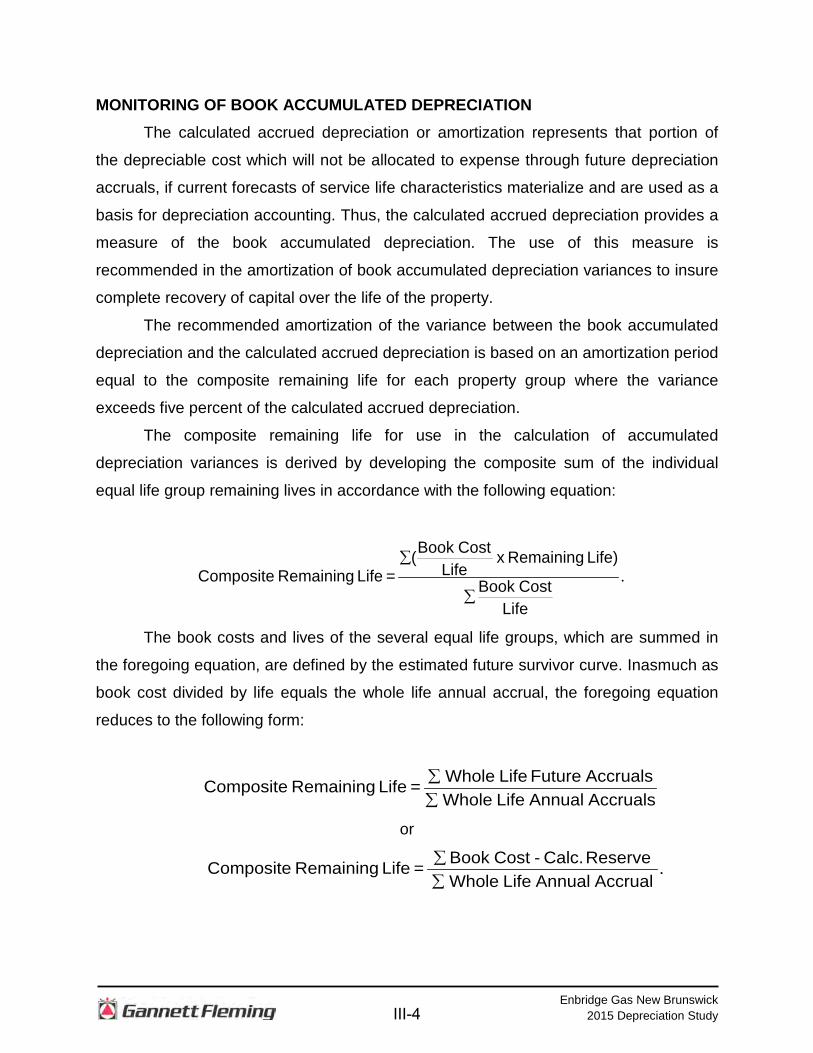
The composite remaining life for use in the calculation of accumulated
depreciation variances is derived by developing the composite sum of the individual
equal life group remaining lives in accordance with the following equation:
.
LifeCost Book
Life) Remaining x Life
Cost Book( = Life Remaining Composite
∑
∑
The book costs and lives of the several equal life groups, which are summed in
the foregoing equation, are defined by the estimated future survivor curve. Inasmuch as
book cost divided by life equals the whole life annual accrual, the foregoing equation
reduces to the following form:
Accruals AnnualLife Whole AccrualsFuture Life Whole = Life Remaining Composite
∑∑
or
. Accrual AnnualLife Whole
Reserve Calc. - Cost Book = Life Remaining Composite∑∑
III-4
Enbridge Gas New Brunswick 2015 Depreciation Study
For the purposes of calculating remaining life accrual rates, the book
depreciation reserve for each plant account is allocated among vintages in proportion to
the calculated accrued depreciation for the account. The calculated accrued
depreciation for each depreciable property group represents that portion of the
depreciable cost of the group which would not be allocated to expense through future
depreciation accruals if current forecasts of service life characteristics materialize and
are used as a basis for depreciation accounting.
In the average life group procedure, the remaining life annual accrual for each
vintage is determined by dividing future book accruals (original cost less book reserve)
by the average remaining life for the surviving original cost of that vintage. The average
remaining life is defined by the estimated future survivor curve.
The annual accrual rate for each account is equal to the sum of the remaining life
annual accruals divided by the total original cost. The composite remaining life is
calculated by dividing the sum of the future book accruals by the sum of the remaining
life annual accruals.
III-5
Enbridge Gas New Brunswick 2015 Depreciation Study
PART IV. RESULTS OF STUDY
IV-1
Enbridge Gas New Brunswick 2015 Depreciation Study
PART IV. RESULTS OF STUDY
QUALIFICATION OF RESULTS
The calculated annual and accrued depreciation are the principal results of the
study. Continued surveillance and periodic revisions are normally required to maintain
continued use of appropriate annual depreciation accrual rates. An assumption that
accrual rates can remain unchanged over a long period of time implies a disregard for
the inherent variability in service lives and for the change of the composition of property
in service. The annual accrual rates and the accrued depreciation were calculated in
accordance with the straight line method, using the equal life group procedure based on
estimates which reflect considerations of current historical evidence and expected future
conditions.
DESCRIPTION OF DETAILED TABULATIONS
The service life estimates were based on judgment that incorporated statistical
analysis of retirement data, discussions with management and consideration of
estimates made for other gas distribution utilities. The results of the statistical analysis
of service life are presented in the section beginning on page V-2 of this report.
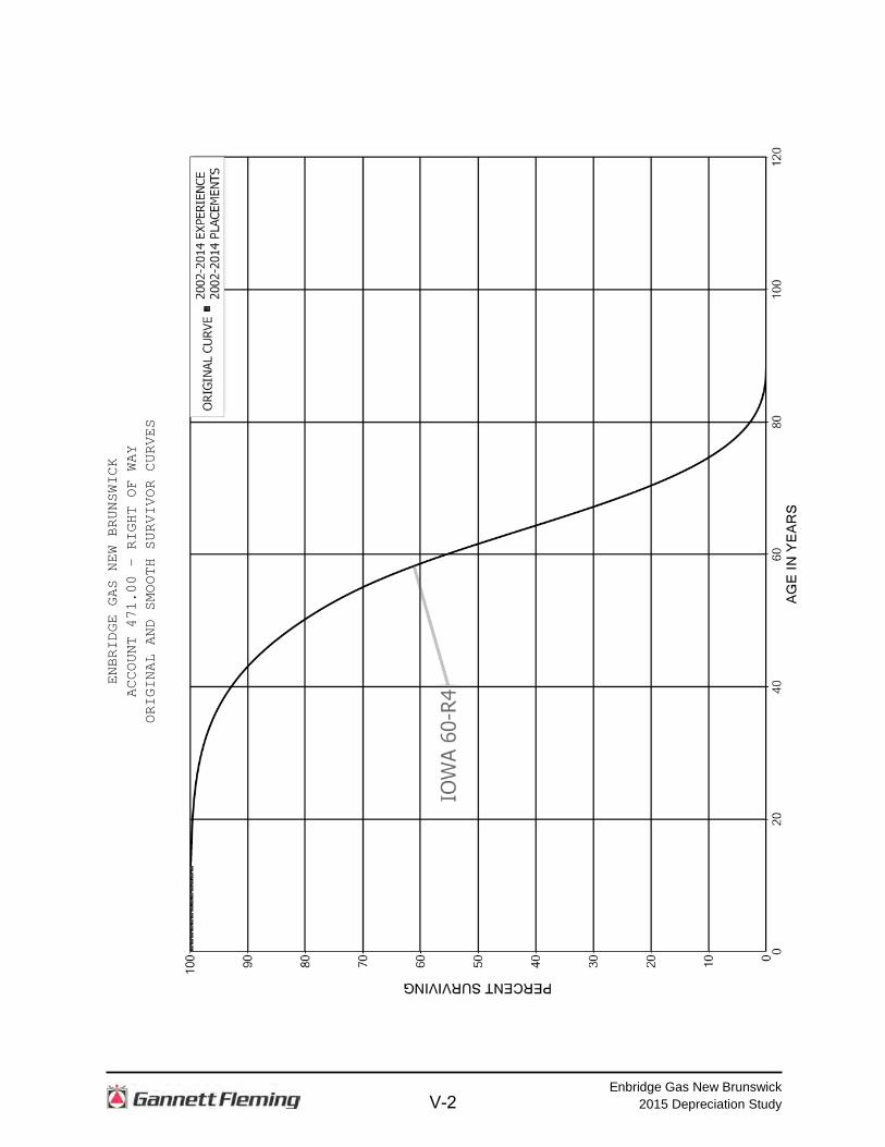
For each depreciable group analyzed by the retirement rate method, a chart
depicting the original and estimated survivor curves followed by a tabular presentation
of the original life table(s) plotted on the chart. The survivor curves estimated for the
depreciable groups are shown as dark smooth curves on the charts. Each smooth
survivor curve is denoted by a numeral followed by the curve type designation. The
numeral used is the average life derived from the entire curve from 100 percent to zero
percent surviving. The titles of the chart indicate the group, the symbol used to plot the
points of the original life table, and the experience and placement bands of the life
tables which where plotted. The experience band indicates the range of years for which
retirements were used to develop the stub survivor curve. The placements indicate, for
the related experience band, the range of years of installations which appear in the
experience.
The tables of the calculated annual depreciation applicable to depreciable assets
as of December 31, 2014 are presented in account sequence starting on page VII-2 of
IV-2
Enbridge Gas New Brunswick 2015 Depreciation Study
the supporting documents. The tables indicate the estimated average survivor curves
used in the calculations. The tables set forth, for each installation year, the original cost,
calculated accrued depreciation, and the calculated annual accrual.
IV-3
Enbridge Gas New Brunswick 2015 Depreciation Study
O
RIG
INAL
CO
STB
OO
KC
OM
POSI
TESU
RVI
VOR
NET
AS O
FD
EPR
ECIA
TIO
NFU
TUR
EAC
CR
UAL
ACC
RU
AL
REM
AIN
ING
AC
CO
UN
TAC
CO
UN
T D
ESC
RIP
TIO
NC
UR
VESA
LVAG
E (%
)D
ECEM
BER
31,
201
4R
ESER
VEAC
CR
UAL
SAM
OU
NT
RAT
ELI
FE(1
)(2
)(3
)(4
)(5
)(6
)(7
)(8
)=(7
)/(4)
(9)=
(6)/(
7)D
ISTR
IBU
TIO
N P
LAN
T47
1.00
RIG
HT
OF
WA
Y60
-R4
-
18
9,28
3
-
18
9,28
3
4,
037
2.
13
46.9
47
3.00
SE
RV
ICE
S60
-R2.
5-
59,0
59,9
77
14,5
29,1
07
44,5
30,8
70
1,02
6,20
9
1.74
43
.4
475.
00
M
AIN
S65
-R3
-
12
2,13
1,82
7
24,2
25,1
32
97,9
06,6
95
2,00
3,09
7
1.64
48
.9
477.
01
S
TATI
ON
S35
-S3
-
15
,415
,662
5,
187,
017
10,2
28,6
45
434,
620
2.82
23
.5
477.
02
M
ETE
RS
AN
D R
EG
ULA
TOR
S20
-S0.
5-
21,8
89,8
65
3,88
7,41
5
18
,002
,451
1,
669,
732
7.
63
10.8
TOTA
L D
ISTR
IBU
TIO
N P
LAN
T21
8,68
6,61
4
47,8
28,6
70
170,
857,
944
5,13
7,69
5
2.35
GEN
ERAL
PLA
NT
483.
00
O
FFIC
E F
UR
NIT
UR
E A
ND
EQ
UIP
ME
NT
20-S
Q-
463,
808
20
6,07
3
257,
735
29,7
36
6.
41
8.7
484.
00
TR
AN
SP
OR
TATI
ON
EQ
UIP
ME
NT
8-S
315
1,39
6,57
9
87
9,78
7
307,
305
88,3
08
6.
32
3.5
486.
00
TO
OLS
AN
D W
OR
K E
QU
IPM
EN
T10
-SQ
-
1,
696,
779
485,
394
1,
211,
385
24
6,57
0
14
.53
4.9
488.
00
C
OM
MU
NIC
ATI
ON
S E
QU
IPM
EN
T10
-SQ
-
81
,156
81,1
56
-
-
-
-
490.
00
C
OM
PU
TER
HA
RD
WA
RE
5-S
Q-
940,
391
77
7,96
2
162,
429
83,4
32
8.
87
1.9
491.
50
C
OM
PU
TER
SO
FTW
AR
E7-
SQ
-
40
9,94
4
370,
635
39
,310
10
,678
2.60
3.
7
49
1.60
INTA
NG
IBLE
SO
FTW
AR
E5-
SQ
-
1,
935,
446
1,74
3,92
1
19
1,52
5
95
,948
4.96
2.
0
TOTA
L G
ENER
AL P
LAN
T6,
924,
104
4,54
4,92
8
2,
169,
689
55
4,67
2
8.
01
TOTA
L D
EPR
ECIA
BLE
PLA
NT
225,
610,
718
52
,373
,598
17
3,02
7,63
3
5,
692,
367
2.
52
PLAN
T N
OT
STU
DIE
D47
0.00
LAN
D37
4,96
7
5,76
9,85
0
47
5.90
DE
VE
LOP
ME
NT
OP
ER
ATI
ON
AN
D M
AIN
TEN
AN
CE
-
11
4,90
1,73
3
20,5
42,2
89
482.
00
LE
AS
EH
OLD
IMP
RO
VE
ME
NTS
-
93
3,14
6
612,
115
TOTA
L PL
ANT
NO
T ST
UD
IED
116,
209,
846
26
,924
,254
TOTA
L PL
ANT
341,
820,
564
79
,297
,852
17
3,02
7,63
3
5,
692,
367
ENB
RID
GE
GAS
NEW
BR
UN
SWIC
K
TAB
LE 1
. ES
TIM
ATED
SU
RVI
VOR
CU
RVE
, OR
IGIN
AL C
OST
, BO
OK
DEP
REC
IATI
ON
RES
ERVE
AN
D C
ALC
ULA
TED
ANN
UAL
DEP
REC
IATI
ON
AC
CR
UAL
S R
ELAT
ED T
O U
TILI
TY P
LAN
T AS
OF
DEC
EMB
ER 3
1, 2
014
DEP
REC
IATI
ON
REL
ATED
TO
REC
OVE
RY
OF
OR
IGIN
AL C
OST
OF
INVE
STM
ENT
CAL
CU
LATE
D A
NN
UAL
IV-4
Enbridge Gas New Brunswick 2015 Depreciation Study
PART V. SERVICE LIFE STATISTICS
V-1
Enbridge Gas New Brunswick 2015 Depreciation Study
ENBRIDGE GAS NEW BRUNSWICK
ACCOUNT 471.00 - RIGHT OF WAY
ORIGINAL AND SMOOTH SURVIVOR CURVES
V-2
Enbridge Gas New Brunswick 2015 Depreciation Study
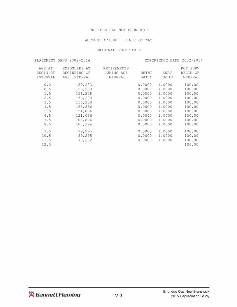
ENBRIDGE GAS NEW BRUNSWICK
ACCOUNT 471.00 - RIGHT OF WAY
ORIGINAL LIFE TABLE
PLACEMENT BAND 2002-2014 EXPERIENCE BAND 2002-2014
AGE AT EXPOSURES AT RETIREMENTS PCT SURV BEGIN OF BEGINNING OF DURING AGE RETMT SURV BEGIN OF INTERVAL AGE INTERVAL INTERVAL RATIO RATIO INTERVAL
0.0 189,283 0.0000 1.0000 100.00 0.5 156,208 0.0000 1.0000 100.00 1.5 156,208 0.0000 1.0000 100.00 2.5 156,208 0.0000 1.0000 100.00 3.5 156,208 0.0000 1.0000 100.00 4.5 155,866 0.0000 1.0000 100.00 5.5 121,066 0.0000 1.0000 100.00 6.5 121,066 0.0000 1.0000 100.00 7.5 108,826 0.0000 1.0000 100.00 8.5 107,394 0.0000 1.0000 100.00
9.5 99,295 0.0000 1.0000 100.00 10.5 89,295 0.0000 1.0000 100.00 11.5 70,652 0.0000 1.0000 100.00 12.5 100.00
V-3
Enbridge Gas New Brunswick 2015 Depreciation Study
ENBRIDGE GAS NEW BRUNSWICK
ACCOUNT 473.00 - SERVICES
ORIGINAL AND SMOOTH SURVIVOR CURVES
V-4
Enbridge Gas New Brunswick 2015 Depreciation Study
ENBRIDGE GAS NEW BRUNSWICK
ACCOUNT 473.00 - SERVICES
ORIGINAL LIFE TABLE
PLACEMENT BAND 2002-2014 EXPERIENCE BAND 2002-2014
AGE AT EXPOSURES AT RETIREMENTS PCT SURV BEGIN OF BEGINNING OF DURING AGE RETMT SURV BEGIN OF INTERVAL AGE INTERVAL INTERVAL RATIO RATIO INTERVAL
0.0 9,410,873 0.0000 1.0000 100.00 0.5 56,481,471 0.0000 1.0000 100.00 1.5 53,488,436 2,590 0.0000 1.0000 100.00 2.5 47,886,643 377 0.0000 1.0000 100.00 3.5 44,086,272 38,046 0.0009 0.9991 99.99 4.5 39,788,485 101,479 0.0026 0.9974 99.91 5.5 35,484,631 15,581 0.0004 0.9996 99.65 6.5 30,632,277 60,744 0.0020 0.9980 99.61 7.5 24,539,240 89,432 0.0036 0.9964 99.41 8.5 20,179,291 38,350 0.0019 0.9981 99.05
9.5 12,968,069 52,111 0.0040 0.9960 98.86 10.5 9,312,856 0.0000 1.0000 98.46 11.5 4,687,348 0.0000 1.0000 98.46 12.5 98.46
V-5
Enbridge Gas New Brunswick 2015 Depreciation Study
ENBRIDGE GAS NEW BRUNSWICK
ACCOUNT 475.00 - MAINS
ORIGINAL AND SMOOTH SURVIVOR CURVES
V-6
Enbridge Gas New Brunswick 2015 Depreciation Study
ENBRIDGE GAS NEW BRUNSWICK
ACCOUNT 475.00 - MAINS
ORIGINAL LIFE TABLE
PLACEMENT BAND 2001-2014 EXPERIENCE BAND 2001-2014
AGE AT EXPOSURES AT RETIREMENTS PCT SURV BEGIN OF BEGINNING OF DURING AGE RETMT SURV BEGIN OF INTERVAL AGE INTERVAL INTERVAL RATIO RATIO INTERVAL
0.0 42,263,097 0.0000 1.0000 100.00 0.5 141,164,357 0.0000 1.0000 100.00 1.5 138,590,469 955,989 0.0069 0.9931 100.00 2.5 128,383,262 0.0000 1.0000 99.31 3.5 122,693,353 0.0000 1.0000 99.31 4.5 116,225,175 0.0000 1.0000 99.31 5.5 86,884,548 0.0000 1.0000 99.31 6.5 71,512,902 0.0000 1.0000 99.31 7.5 63,307,661 0.0000 1.0000 99.31 8.5 61,211,876 0.0000 1.0000 99.31
9.5 47,198,253 0.0000 1.0000 99.31 10.5 33,357,136 0.0000 1.0000 99.31 11.5 20,646,659 0.0000 1.0000 99.31 12.5 9,406,942 0.0000 1.0000 99.31 13.5 99.31
V-7
Enbridge Gas New Brunswick 2015 Depreciation Study
ENBRIDGE GAS NEW BRUNSWICK
ACCOUNT 477.01 - STATIONS
ORIGINAL AND SMOOTH SURVIVOR CURVES
V-8
Enbridge Gas New Brunswick 2015 Depreciation Study
ENBRIDGE GAS NEW BRUNSWICK
ACCOUNT 477.01 - STATIONS
ORIGINAL LIFE TABLE
PLACEMENT BAND 2002-2014 EXPERIENCE BAND 2002-2014
AGE AT EXPOSURES AT RETIREMENTS PCT SURV BEGIN OF BEGINNING OF DURING AGE RETMT SURV BEGIN OF INTERVAL AGE INTERVAL INTERVAL RATIO RATIO INTERVAL
0.0 2,566,707 13,638 0.0053 0.9947 100.00 0.5 15,214,218 0.0000 1.0000 99.47 1.5 15,032,298 0.0000 1.0000 99.47 2.5 14,355,322 3,982 0.0003 0.9997 99.47 3.5 14,125,458 0.0000 1.0000 99.44 4.5 13,305,824 0.0000 1.0000 99.44 5.5 12,373,786 0.0000 1.0000 99.44 6.5 9,069,801 0.0000 1.0000 99.44 7.5 8,683,454 0.0000 1.0000 99.44 8.5 7,847,922 0.0000 1.0000 99.44
9.5 5,580,105 0.0000 1.0000 99.44 10.5 2,583,902 136 0.0001 0.9999 99.44 11.5 1,778,345 0.0000 1.0000 99.44 12.5 99.44
V-9
Enbridge Gas New Brunswick 2015 Depreciation Study
ENBRIDGE GAS NEW BRUNSWICK
ACCOUNT 477.02 – METERS AND REGULATORS
ORIGINAL AND SMOOTH SURVIVOR CURVES
V-10
Enbridge Gas New Brunswick 2015 Depreciation Study
ENBRIDGE GAS NEW BRUNSWICK
ACCOUNT 477.02 – METERS AND REGULATORS
ORIGINAL LIFE TABLE
PLACEMENT BAND 2002-2014 EXPERIENCE BAND 2002-2014
AGE AT EXPOSURES AT RETIREMENTS PCT SURV BEGIN OF BEGINNING OF DURING AGE RETMT SURV BEGIN OF INTERVAL AGE INTERVAL INTERVAL RATIO RATIO INTERVAL
0.0 2,240,109 55,543 0.0248 0.9752 100.00 0.5 22,051,895 82,783 0.0038 0.9962 97.52 1.5 20,387,228 133,609 0.0066 0.9934 97.15 2.5 18,133,956 100,722 0.0056 0.9944 96.52 3.5 15,540,119 72,717 0.0047 0.9953 95.98 4.5 13,918,226 73,540 0.0053 0.9947 95.53 5.5 12,785,676 175,460 0.0137 0.9863 95.03 6.5 11,660,597 110,405 0.0095 0.9905 93.72 7.5 10,201,676 87,107 0.0085 0.9915 92.84 8.5 8,238,496 714,535 0.0867 0.9133 92.04
9.5 6,333,034 226,879 0.0358 0.9642 84.06 10.5 3,244,907 62,855 0.0194 0.9806 81.05 11.5 2,005,774 49,913 0.0249 0.9751 79.48 12.5 77.50
V-11
Enbridge Gas New Brunswick 2015 Depreciation Study
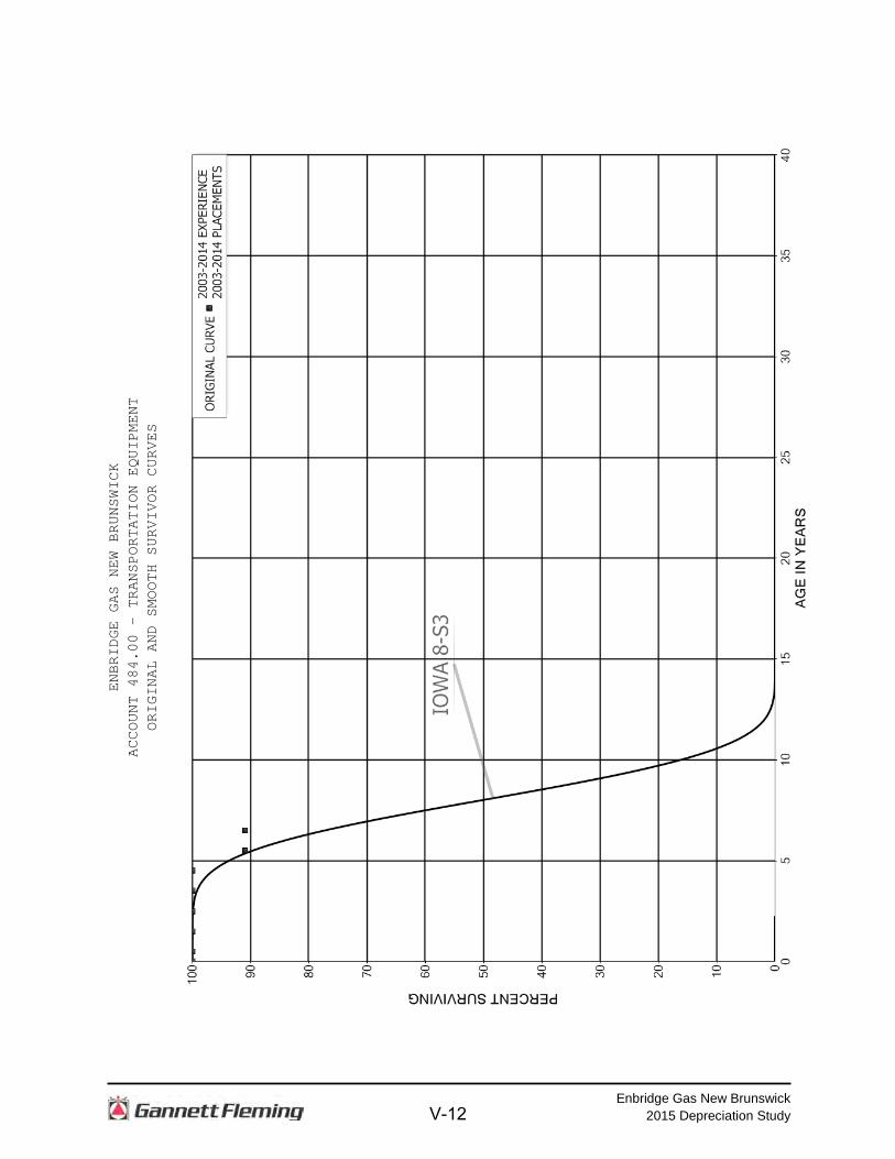
ENBRIDGE GAS NEW BRUNSWICK
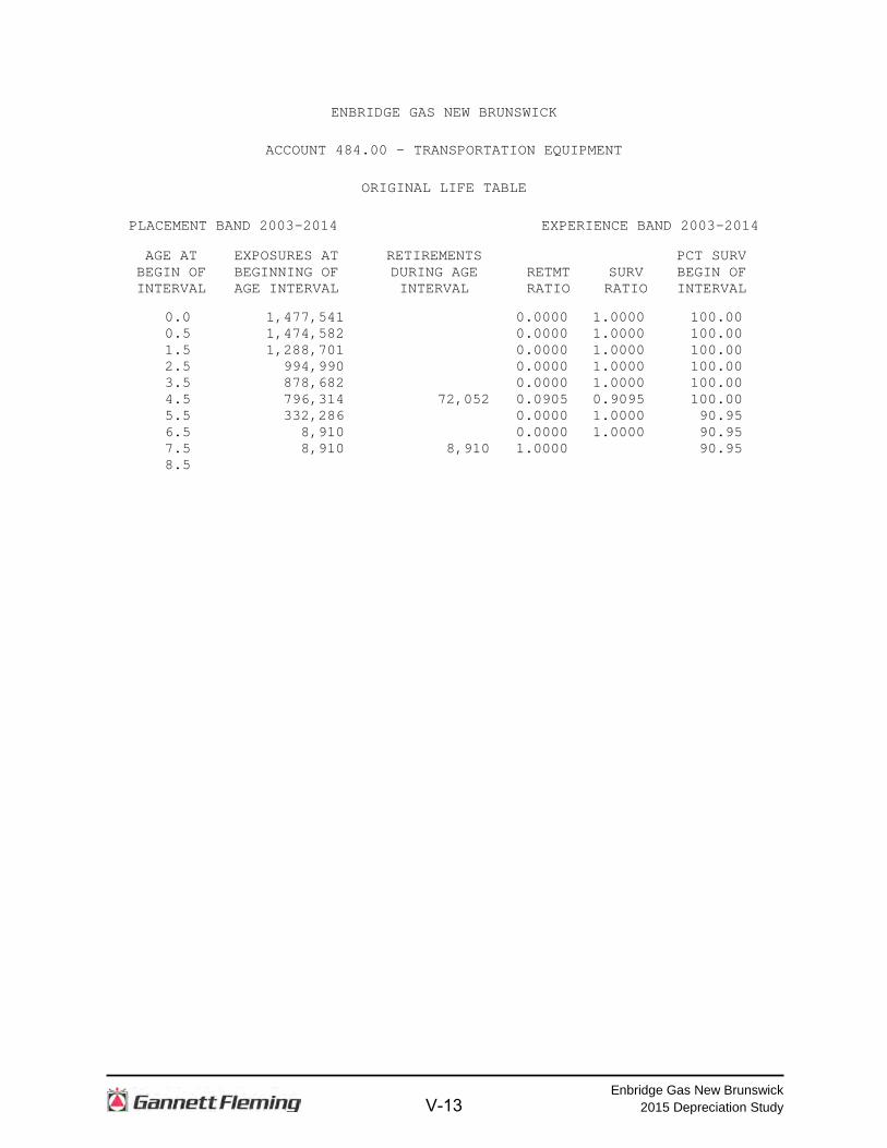
ACCOUNT 484.00 - TRANSPORTATION EQUIPMENT
ORIGINAL AND SMOOTH SURVIVOR CURVES
V-12
Enbridge Gas New Brunswick 2015 Depreciation Study
ENBRIDGE GAS NEW BRUNSWICK
ACCOUNT 484.00 - TRANSPORTATION EQUIPMENT
ORIGINAL LIFE TABLE
PLACEMENT BAND 2003-2014 EXPERIENCE BAND 2003-2014
AGE AT EXPOSURES AT RETIREMENTS PCT SURV BEGIN OF BEGINNING OF DURING AGE RETMT SURV BEGIN OF INTERVAL AGE INTERVAL INTERVAL RATIO RATIO INTERVAL
0.0 1,477,541 0.0000 1.0000 100.00 0.5 1,474,582 0.0000 1.0000 100.00 1.5 1,288,701 0.0000 1.0000 100.00 2.5 994,990 0.0000 1.0000 100.00 3.5 878,682 0.0000 1.0000 100.00 4.5 796,314 72,052 0.0905 0.9095 100.00 5.5 332,286 0.0000 1.0000 90.95 6.5 8,910 0.0000 1.0000 90.95 7.5 8,910 8,910 1.0000 90.95 8.5
V-13
Enbridge Gas New Brunswick 2015 Depreciation Study
PART VI. DETAILED DEPRECIATIONS CALCULATIONS
VI-1
Enbridge Gas New Brunswick 2015 Depreciation Study
ENBRIDGE GAS NEW BRUNSWICK
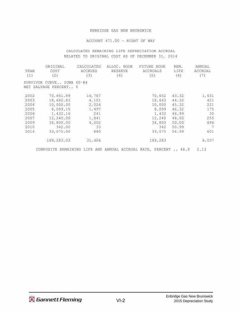
ACCOUNT 471.00 - RIGHT OF WAY
CALCULATED REMAINING LIFE DEPRECIATION ACCRUAL
RELATED TO ORIGINAL COST AS OF DECEMBER 31, 2014 ORIGINAL CALCULATED ALLOC. BOOK FUTURE BOOK REM. ANNUAL
YEAR COST ACCRUED RESERVE ACCRUALS LIFE ACCRUAL (1) (2) (3) (4) (5) (6) (7)
SURVIVOR CURVE.. IOWA 60-R4 NET SALVAGE PERCENT.. 0 2002 70,651.89 16,787 70,652 43.32 1,631 2003 18,642.83 4,101 18,643 44.32 421 2004 10,000.00 2,024 10,000 45.32 221 2005 8,099.15 1,497 8,099 46.32 175 2006 1,432.16 241 1,432 46.99 30 2007 12,240.00 1,841 12,240 48.00 255 2009 34,800.00 4,002 34,800 50.00 696 2010 342.00 33 342 50.99 7 2014 33,075.00 880 33,075 54.99 601 189,283.03 31,406 189,283 4,037
COMPOSITE REMAINING LIFE AND ANNUAL ACCRUAL RATE, PERCENT .. 46.9 2.13
VI-2
Enbridge Gas New Brunswick 2015 Depreciation Study
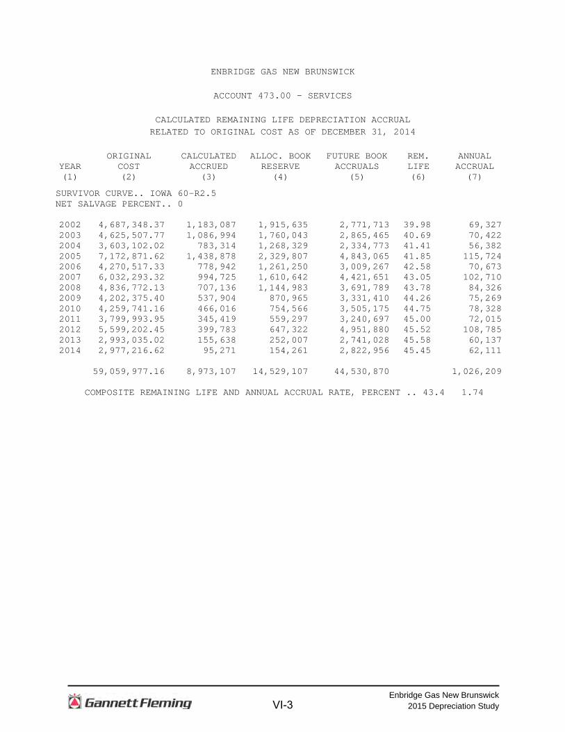
ENBRIDGE GAS NEW BRUNSWICK
ACCOUNT 473.00 - SERVICES
CALCULATED REMAINING LIFE DEPRECIATION ACCRUAL
RELATED TO ORIGINAL COST AS OF DECEMBER 31, 2014 ORIGINAL CALCULATED ALLOC. BOOK FUTURE BOOK REM. ANNUAL
YEAR COST ACCRUED RESERVE ACCRUALS LIFE ACCRUAL (1) (2) (3) (4) (5) (6) (7)
SURVIVOR CURVE.. IOWA 60-R2.5 NET SALVAGE PERCENT.. 0 2002 4,687,348.37 1,183,087 1,915,635 2,771,713 39.98 69,327 2003 4,625,507.77 1,086,994 1,760,043 2,865,465 40.69 70,422 2004 3,603,102.02 783,314 1,268,329 2,334,773 41.41 56,382 2005 7,172,871.62 1,438,878 2,329,807 4,843,065 41.85 115,724 2006 4,270,517.33 778,942 1,261,250 3,009,267 42.58 70,673 2007 6,032,293.32 994,725 1,610,642 4,421,651 43.05 102,710 2008 4,836,772.13 707,136 1,144,983 3,691,789 43.78 84,326 2009 4,202,375.40 537,904 870,965 3,331,410 44.26 75,269 2010 4,259,741.16 466,016 754,566 3,505,175 44.75 78,328 2011 3,799,993.95 345,419 559,297 3,240,697 45.00 72,015 2012 5,599,202.45 399,783 647,322 4,951,880 45.52 108,785 2013 2,993,035.02 155,638 252,007 2,741,028 45.58 60,137 2014 2,977,216.62 95,271 154,261 2,822,956 45.45 62,111 59,059,977.16 8,973,107 14,529,107 44,530,870 1,026,209
COMPOSITE REMAINING LIFE AND ANNUAL ACCRUAL RATE, PERCENT .. 43.4 1.74
VI-3
Enbridge Gas New Brunswick 2015 Depreciation Study
ENBRIDGE GAS NEW BRUNSWICK
ACCOUNT 475.00 - MAINS
CALCULATED REMAINING LIFE DEPRECIATION ACCRUAL
RELATED TO ORIGINAL COST AS OF DECEMBER 31, 2014 ORIGINAL CALCULATED ALLOC. BOOK FUTURE BOOK REM. ANNUAL
YEAR COST ACCRUED RESERVE ACCRUALS LIFE ACCRUAL (1) (2) (3) (4) (5) (6) (7)
SURVIVOR CURVE.. IOWA 65-R3 NET SALVAGE PERCENT.. 0 2001 9,406,941.80 2,304,701 2,901,219 6,505,723 44.67 145,640 2002 11,239,717.58 2,579,515 3,247,163 7,992,555 45.32 176,358 2003 12,710,476.28 2,700,976 3,400,061 9,310,415 46.32 201,002 2004 13,841,116.84 2,721,164 3,425,474 10,415,643 46.98 221,704 2005 14,013,623.85 2,530,860 3,185,915 10,827,709 47.64 227,282 2006 2,095,784.67 342,451 431,086 1,664,699 48.64 34,225 2007 8,205,240.73 1,206,170 1,518,359 6,686,882 49.31 135,609 2008 15,371,646.52 1,995,240 2,511,662 12,859,985 50.30 255,666 2009 9,273,047.06 1,048,782 1,320,235 7,952,812 50.97 156,029 2010 6,468,177.81 622,239 783,291 5,684,887 51.65 110,066 2011 5,689,908.78 450,641 567,279 5,122,630 52.32 97,910 2012 9,251,218.32 573,576 722,033 8,529,185 52.99 160,958 2013 2,573,888.06 114,538 144,184 2,429,704 53.68 45,263 2014 1,991,038.35 53,360 67,171 1,923,868 54.37 35,385 122,131,826.65 19,244,213 24,225,132 97,906,695 2,003,097
COMPOSITE REMAINING LIFE AND ANNUAL ACCRUAL RATE, PERCENT .. 48.9 1.64
VI-4
Enbridge Gas New Brunswick 2015 Depreciation Study
ENBRIDGE GAS NEW BRUNSWICK
ACCOUNT 477.01 - STATIONS
CALCULATED REMAINING LIFE DEPRECIATION ACCRUAL
RELATED TO ORIGINAL COST AS OF DECEMBER 31, 2014 ORIGINAL CALCULATED ALLOC. BOOK FUTURE BOOK REM. ANNUAL
YEAR COST ACCRUED RESERVE ACCRUALS LIFE ACCRUAL (1) (2) (3) (4) (5) (6) (7)
SURVIVOR CURVE.. IOWA 35-S3 NET SALVAGE PERCENT.. 0 2002 1,778,344.92 729,833 865,926 912,419 19.39 47,056 2003 805,421.11 307,027 364,279 441,142 20.29 21,742 2004 2,996,203.54 1,054,364 1,250,972 1,745,232 21.18 82,400 2005 2,267,816.57 728,649 864,521 1,403,296 22.18 63,269 2006 835,531.77 242,889 288,181 547,351 23.18 23,613 2007 386,347.00 100,489 119,227 267,120 24.18 11,047 2008 3,303,985.63 758,265 899,660 2,404,326 25.18 95,486 2009 932,038.03 185,382 219,950 712,088 26.18 27,200 2010 819,633.25 137,944 163,667 655,966 27.18 24,134 2011 225,883.03 31,104 36,904 188,979 28.18 6,706 2012 676,975.82 72,504 86,024 590,952 29.18 20,252 2013 181,919.56 13,917 16,512 165,408 30.18 5,481 2014 205,561.83 9,435 11,194 194,368 31.18 6,234 15,415,662.06 4,371,802 5,187,017 10,228,645 434,620
COMPOSITE REMAINING LIFE AND ANNUAL ACCRUAL RATE, PERCENT .. 23.5 2.82
VI-5
Enbridge Gas New Brunswick 2015 Depreciation Study
ENBRIDGE GAS NEW BRUNSWICK
ACCOUNT 477.02 - METERS AND REGULATORS
CALCULATED REMAINING LIFE DEPRECIATION ACCRUAL
RELATED TO ORIGINAL COST AS OF DECEMBER 31, 2014 ORIGINAL CALCULATED ALLOC. BOOK FUTURE BOOK REM. ANNUAL
YEAR COST ACCRUED RESERVE ACCRUALS LIFE ACCRUAL (1) (2) (3) (4) (5) (6) (7)
SURVIVOR CURVE.. IOWA 20-S0.5 NET SALVAGE PERCENT.. 0 2002 1,955,861.41 1,196,205 549,620 1,406,241 8.57 164,089 2003 1,176,278.83 686,712 315,523 860,756 8.91 96,606 2004 2,861,247.22 1,582,842 727,268 2,133,979 9.29 229,707 2005 1,190,927.19 620,235 284,979 905,948 9.66 93,783 2006 1,876,072.06 912,521 419,276 1,456,796 10.03 145,244 2007 1,348,515.75 606,293 278,573 1,069,943 10.40 102,879 2008 949,619.51 388,869 178,674 770,946 10.82 71,252 2009 1,059,008.91 388,868 178,673 880,336 11.20 78,601 2010 1,549,176.55 498,525 229,057 1,320,120 11.59 113,902 2011 2,493,115.20 679,873 312,381 2,180,734 12.00 181,728 2012 2,119,662.29 465,902 214,068 1,905,594 12.42 153,429 2013 1,581,883.56 257,847 118,473 1,463,411 12.84 113,973 2014 1,728,496.63 175,961 80,850 1,647,647 13.23 124,539 21,889,865.11 8,460,653 3,887,415 18,002,451 1,669,732
COMPOSITE REMAINING LIFE AND ANNUAL ACCRUAL RATE, PERCENT .. 10.8 7.63
VI-6
Enbridge Gas New Brunswick 2015 Depreciation Study
ENBRIDGE GAS NEW BRUNSWICK
ACCOUNT 483.00 - OFFICE FURNITURE AND EQUIPMENT
CALCULATED REMAINING LIFE DEPRECIATION ACCRUAL
RELATED TO ORIGINAL COST AS OF DECEMBER 31, 2014 ORIGINAL CALCULATED ALLOC. BOOK FUTURE BOOK REM. ANNUAL
YEAR COST ACCRUED RESERVE ACCRUALS LIFE ACCRUAL (1) (2) (3) (4) (5) (6) (7)
SURVIVOR CURVE.. 20-SQUARE NET SALVAGE PERCENT.. 0 2002 137,885.19 93,073 74,518 63,367 6.50 9,749 2003 143,210.49 89,507 71,662 71,548 7.50 9,540 2004 7,862.02 4,521 3,620 4,242 8.50 499 2005 7,677.13 4,030 3,227 4,450 9.50 468 2006 20,033.31 9,516 7,619 12,414 10.50 1,182 2007 85,525.60 36,348 29,101 56,425 11.50 4,907 2008 39,697.86 14,887 11,919 27,779 12.50 2,222 2009 1,422.14 462 370 1,052 13.50 78 2010 9,296.30 2,556 2,046 7,250 14.50 500 2011 10,538.89 2,371 1,899 8,640 15.50 557 2012 659.03 115 92 567 16.50 34 463,807.96 257,386 206,073 257,735 29,736
COMPOSITE REMAINING LIFE AND ANNUAL ACCRUAL RATE, PERCENT .. 8.7 6.41
VI-7
Enbridge Gas New Brunswick 2015 Depreciation Study
ENBRIDGE GAS NEW BRUNSWICK
ACCOUNT 484.00 - TRANSPORTATION EQUIPMENT
CALCULATED REMAINING LIFE DEPRECIATION ACCRUAL
RELATED TO ORIGINAL COST AS OF DECEMBER 31, 2014 ORIGINAL CALCULATED ALLOC. BOOK FUTURE BOOK REM. ANNUAL
YEAR COST ACCRUED RESERVE ACCRUALS LIFE ACCRUAL (1) (2) (3) (4) (5) (6) (7)
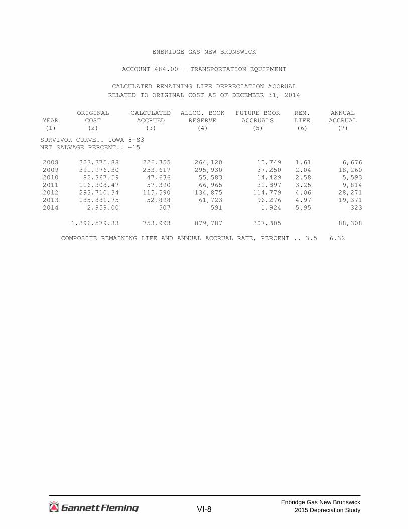
SURVIVOR CURVE.. IOWA 8-S3 NET SALVAGE PERCENT.. +15 2008 323,375.88 226,355 264,120 10,749 1.61 6,676 2009 391,976.30 253,617 295,930 37,250 2.04 18,260 2010 82,367.59 47,636 55,583 14,429 2.58 5,593 2011 116,308.47 57,390 66,965 31,897 3.25 9,814 2012 293,710.34 115,590 134,875 114,779 4.06 28,271 2013 185,881.75 52,898 61,723 96,276 4.97 19,371 2014 2,959.00 507 591 1,924 5.95 323 1,396,579.33 753,993 879,787 307,305 88,308
COMPOSITE REMAINING LIFE AND ANNUAL ACCRUAL RATE, PERCENT .. 3.5 6.32
VI-8
Enbridge Gas New Brunswick 2015 Depreciation Study
ENBRIDGE GAS NEW BRUNSWICK
ACCOUNT 486.00 - TOOLS AND WORK EQUIPMENT
CALCULATED REMAINING LIFE DEPRECIATION ACCRUAL
RELATED TO ORIGINAL COST AS OF DECEMBER 31, 2014 ORIGINAL CALCULATED ALLOC. BOOK FUTURE BOOK REM. ANNUAL
YEAR COST ACCRUED RESERVE ACCRUALS LIFE ACCRUAL (1) (2) (3) (4) (5) (6) (7)
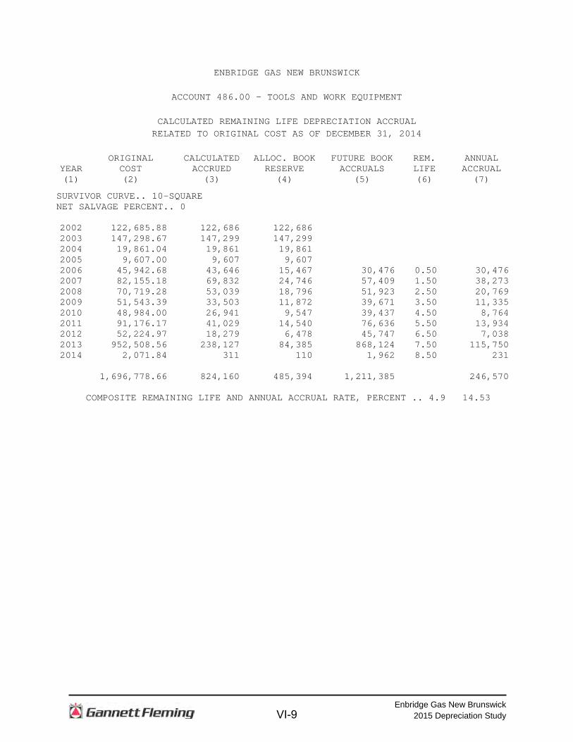
SURVIVOR CURVE.. 10-SQUARE NET SALVAGE PERCENT.. 0 2002 122,685.88 122,686 122,686 2003 147,298.67 147,299 147,299 2004 19,861.04 19,861 19,861 2005 9,607.00 9,607 9,607 2006 45,942.68 43,646 15,467 30,476 0.50 30,476 2007 82,155.18 69,832 24,746 57,409 1.50 38,273 2008 70,719.28 53,039 18,796 51,923 2.50 20,769 2009 51,543.39 33,503 11,872 39,671 3.50 11,335 2010 48,984.00 26,941 9,547 39,437 4.50 8,764 2011 91,176.17 41,029 14,540 76,636 5.50 13,934 2012 52,224.97 18,279 6,478 45,747 6.50 7,038 2013 952,508.56 238,127 84,385 868,124 7.50 115,750 2014 2,071.84 311 110 1,962 8.50 231 1,696,778.66 824,160 485,394 1,211,385 246,570
COMPOSITE REMAINING LIFE AND ANNUAL ACCRUAL RATE, PERCENT .. 4.9 14.53
VI-9
Enbridge Gas New Brunswick 2015 Depreciation Study
ENBRIDGE GAS NEW BRUNSWICK
ACCOUNT 488.00 - COMMUNICATIONS EQUIPMENT
CALCULATED REMAINING LIFE DEPRECIATION ACCRUAL
RELATED TO ORIGINAL COST AS OF DECEMBER 31, 2014 ORIGINAL CALCULATED ALLOC. BOOK FUTURE BOOK REM. ANNUAL
YEAR COST ACCRUED RESERVE ACCRUALS LIFE ACCRUAL (1) (2) (3) (4) (5) (6) (7)
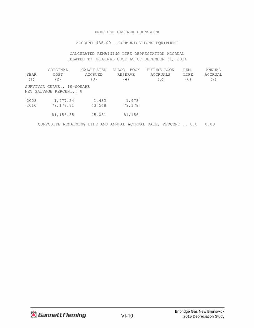
SURVIVOR CURVE.. 10-SQUARE NET SALVAGE PERCENT.. 0 2008 1,977.54 1,483 1,978 2010 79,178.81 43,548 79,178 81,156.35 45,031 81,156
COMPOSITE REMAINING LIFE AND ANNUAL ACCRUAL RATE, PERCENT .. 0.0 0.00
VI-10
Enbridge Gas New Brunswick 2015 Depreciation Study
ENBRIDGE GAS NEW BRUNSWICK
ACCOUNT 490.00 - COMPUTER HARDWARE
CALCULATED REMAINING LIFE DEPRECIATION ACCRUAL
RELATED TO ORIGINAL COST AS OF DECEMBER 31, 2014 ORIGINAL CALCULATED ALLOC. BOOK FUTURE BOOK REM. ANNUAL
YEAR COST ACCRUED RESERVE ACCRUALS LIFE ACCRUAL (1) (2) (3) (4) (5) (6) (7)
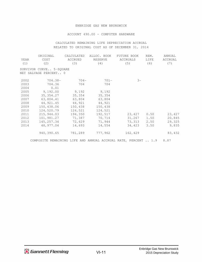
SURVIVOR CURVE.. 5-SQUARE NET SALVAGE PERCENT.. 0 2002 704.38 - 704 - 701 - 3 - 2003 704.36 704 704 2004 0.01 2005 9,192.00 9,192 9,192 2006 35,354.27 35,354 35,354 2007 63,804.41 63,804 63,804 2008 44,921.45 44,921 44,921 2009 150,438.06 150,438 150,438 2010 124,520.79 124,521 124,521 2011 215,944.03 194,350 192,517 23,427 0.50 23,427 2012 101,981.27 71,387 70,714 31,267 1.50 20,845 2013 145,257.34 72,629 71,944 73,313 2.50 29,325 2014 48,977.04 14,693 14,554 34,423 3.50 9,835 940,390.65 781,289 777,962 162,429 83,432
COMPOSITE REMAINING LIFE AND ANNUAL ACCRUAL RATE, PERCENT .. 1.9 8.87
VI-11
Enbridge Gas New Brunswick 2015 Depreciation Study
ENBRIDGE GAS NEW BRUNSWICK
ACCOUNT 491.50 - COMPUTER SOFTWARE
CALCULATED REMAINING LIFE DEPRECIATION ACCRUAL
RELATED TO ORIGINAL COST AS OF DECEMBER 31, 2014 ORIGINAL CALCULATED ALLOC. BOOK FUTURE BOOK REM. ANNUAL
YEAR COST ACCRUED RESERVE ACCRUALS LIFE ACCRUAL (1) (2) (3) (4) (5) (6) (7)
SURVIVOR CURVE.. 7-SQUARE NET SALVAGE PERCENT.. 0 2002 40.00 40 40 2011 194,893.23 125,289 194,893 2012 197,566.85 98,783 165,883 31,684 3.50 9,053 2013 14,765.45 5,273 8,855 5,910 4.50 1,313 2014 2,678.89 574 964 1,715 5.50 312 409,944.42 229,959 370,635 39,310 10,678
COMPOSITE REMAINING LIFE AND ANNUAL ACCRUAL RATE, PERCENT .. 3.7 2.60
VI-12
Enbridge Gas New Brunswick 2015 Depreciation Study
ENBRIDGE GAS NEW BRUNSWICK
ACCOUNT 491.60 - INTANGIBLE SOFTWARE
CALCULATED REMAINING LIFE DEPRECIATION ACCRUAL
RELATED TO ORIGINAL COST AS OF DECEMBER 31, 2014 ORIGINAL CALCULATED ALLOC. BOOK FUTURE BOOK REM. ANNUAL
YEAR COST ACCRUED RESERVE ACCRUALS LIFE ACCRUAL (1) (2) (3) (4) (5) (6) (7)
SURVIVOR CURVE.. 5-SQUARE NET SALVAGE PERCENT.. 0 2009 1,866,037.00 1,866,037 1,866,037 2011 501.02 451 1,405 - 1,906 0.50 1,906 2012 21,448.67 15,014 46,778 - 68,227 1.50 45,485 2013 47,459.59 23,730 73,933 - 121,392 2.50 48,557 1,935,446.28 1,905,232 1,743,921 191,525 95,948
COMPOSITE REMAINING LIFE AND ANNUAL ACCRUAL RATE, PERCENT .. 2.0 4.96
VI-13
Enbridge Gas New Brunswick 2015 Depreciation Study
APPENDIX A ESTIMATION OF SURIVOR CURVES
A-1
Enbridge Gas New Brunswick 2015 Depreciation Study
ESTIMATION OF SURVIVOR CURVES Average Service Life The use of an average service life for a property group implies that the various
units in the group have different lives. Thus, the average life may be obtained by
determining the separate lives of each of the units, or by constructing a survivor curve
by plotting the number of units which survive at successive ages. A discussion of the
general concept of survivor curves is presented. Also, the Iowa type survivor curves are
reviewed.
SURVIVOR CURVES The survivor curve graphically depicts the amount of property existing at each
age throughout the life of an original group. From the survivor curve, the average life of
the group, the remaining life expectancy, the probable life, and the frequency curve can
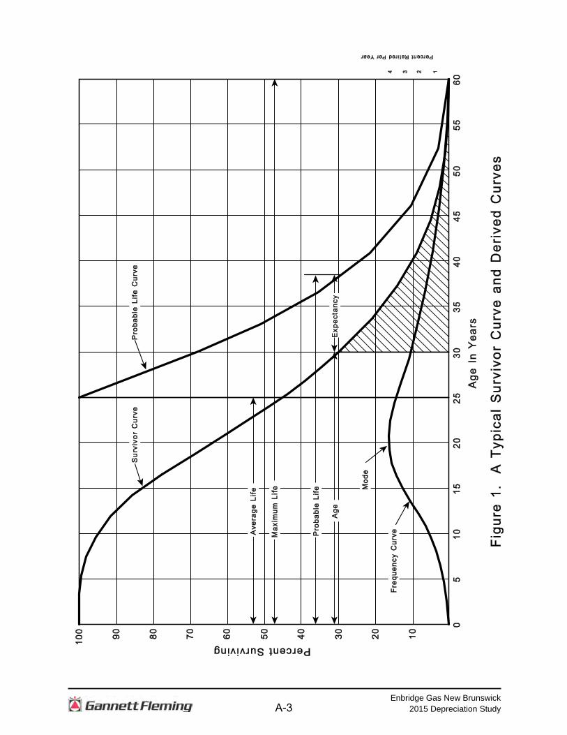
be calculated. In Figure 1, a typical smooth survivor curve and the derived curves are
illustrated. The average life is obtained by calculating the area under the survivor curve,
from age zero to the maximum age, and dividing this area by the ordinate at age zero.
The remaining life expectancy at any age can be calculated by obtaining the area under
the curve, from the observation age to the maximum age, and dividing this area by the
percent surviving at the observation age. For example, in Figure 1, the remaining life at
age 30 is equal to the crosshatched area under the survivor curve divided by 29.5
percent surviving at age 30. The probable life at any age is developed by adding the
age and remaining life. If the probable life of the property is calculated for each year of
age, the probable life curve shown in the chart can be developed. The frequency curve
presents the number of units retired in each age interval. It is derived by obtaining the
differences between the amount of property surviving at the beginning and at the end of
each interval.
Iowa Type Curves The range of survivor characteristics usually experienced by utility and industrial
properties is encompassed by a system of generalized survivor curves known as the
A-2
Enbridge Gas New Brunswick 2015 Depreciation Study
A-3
Enbridge Gas New Brunswick 2015 Depreciation Study
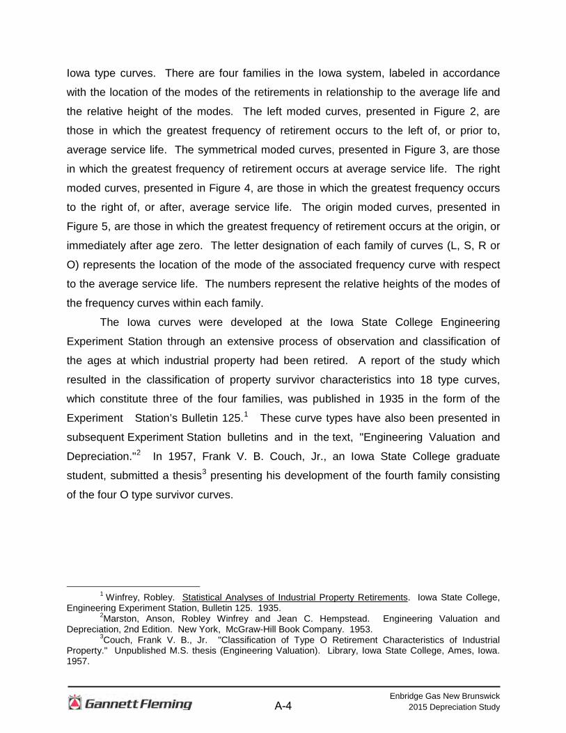
Iowa type curves. There are four families in the Iowa system, labeled in accordance
with the location of the modes of the retirements in relationship to the average life and
the relative height of the modes. The left moded curves, presented in Figure 2, are
those in which the greatest frequency of retirement occurs to the left of, or prior to,
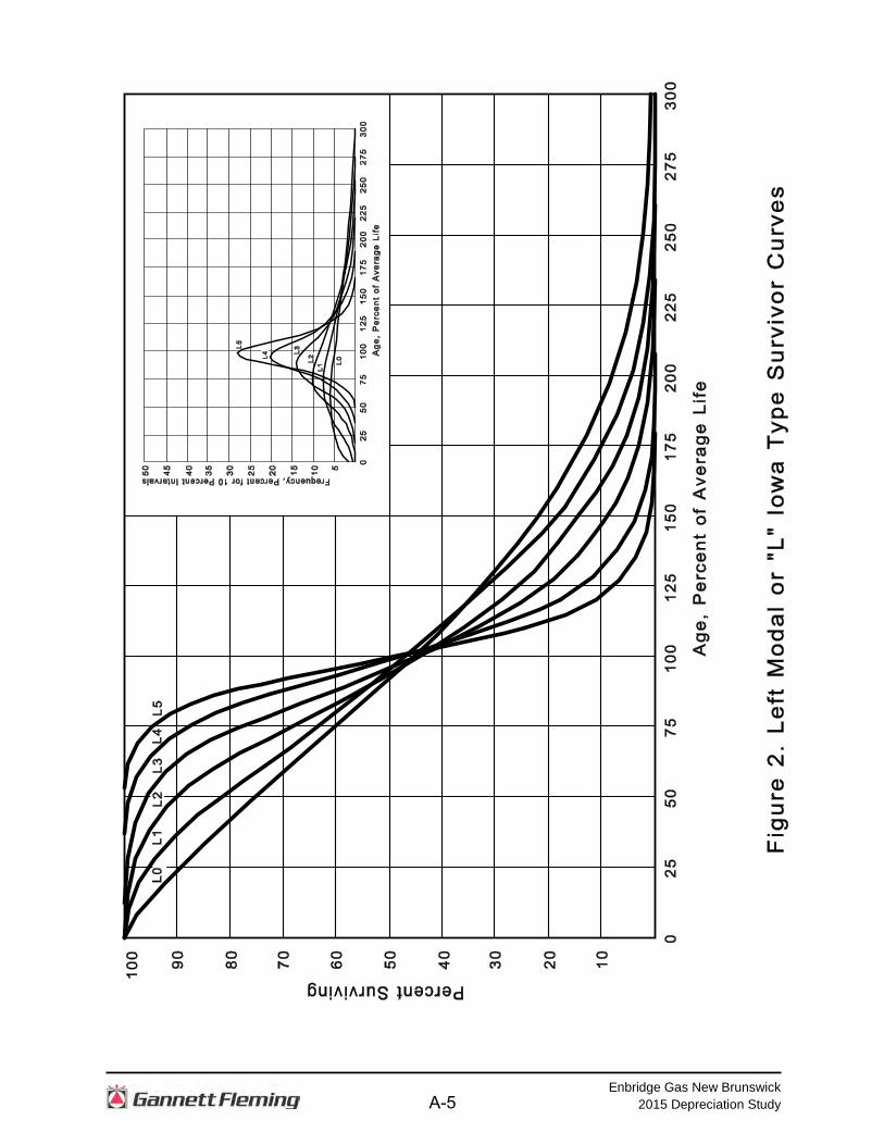
average service life. The symmetrical moded curves, presented in Figure 3, are those
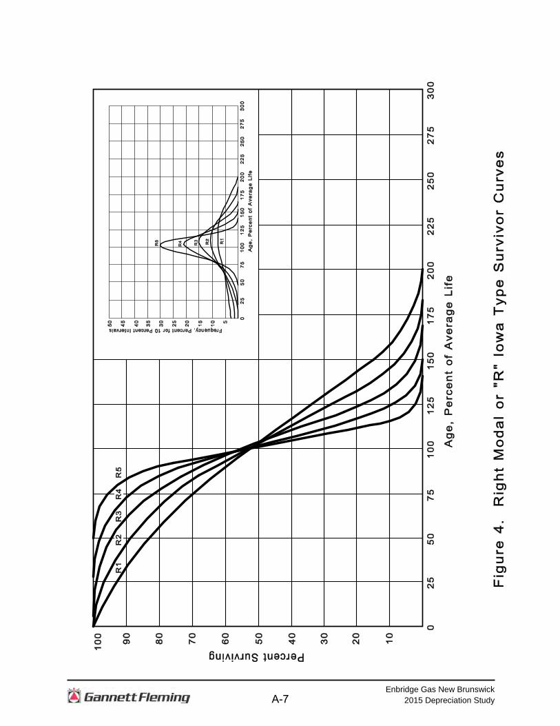
in which the greatest frequency of retirement occurs at average service life. The right
moded curves, presented in Figure 4, are those in which the greatest frequency occurs
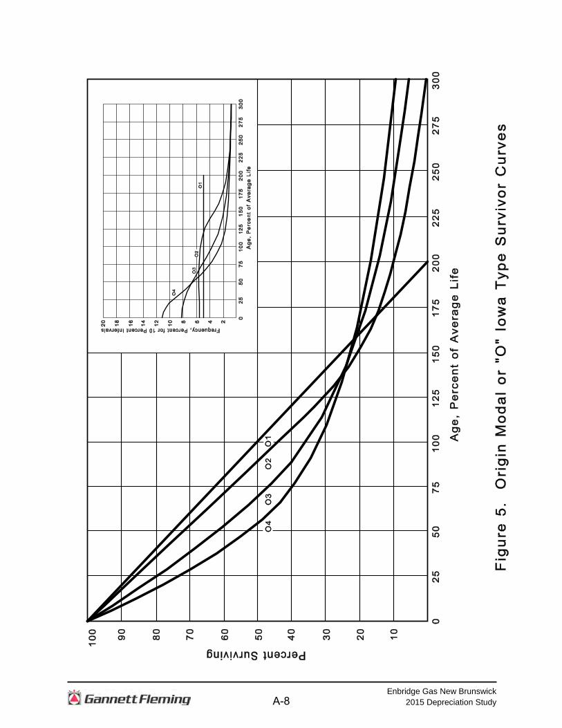
to the right of, or after, average service life. The origin moded curves, presented in
Figure 5, are those in which the greatest frequency of retirement occurs at the origin, or
immediately after age zero. The letter designation of each family of curves (L, S, R or
O) represents the location of the mode of the associated frequency curve with respect
to the average service life. The numbers represent the relative heights of the modes of
the frequency curves within each family.
The Iowa curves were developed at the Iowa State College Engineering
Experiment Station through an extensive process of observation and classification of
the ages at which industrial property had been retired. A report of the study which
resulted in the classification of property survivor characteristics into 18 type curves,
which constitute three of the four families, was published in 1935 in the form of the
Experiment Station’s Bulletin 125.1 These curve types have also been presented in
subsequent Experiment Station bulletins and in the text, "Engineering Valuation and
Depreciation."2 In 1957, Frank V. B. Couch, Jr., an Iowa State College graduate
student, submitted a thesis3 presenting his development of the fourth family consisting
of the four O type survivor curves.
1 Winfrey, Robley. Statistical Analyses of Industrial Property Retirements. Iowa State College, Engineering Experiment Station, Bulletin 125. 1935.
2Marston, Anson, Robley Winfrey and Jean C. Hempstead. Engineering Valuation and Depreciation, 2nd Edition. New York, McGraw-Hill Book Company. 1953.
3Couch, Frank V. B., Jr. "Classification of Type O Retirement Characteristics of Industrial Property." Unpublished M.S. thesis (Engineering Valuation). Library, Iowa State College, Ames, Iowa. 1957.
A-4
Enbridge Gas New Brunswick 2015 Depreciation Study
A-5
Enbridge Gas New Brunswick 2015 Depreciation Study
A-6
Enbridge Gas New Brunswick 2015 Depreciation Study
A-7
Enbridge Gas New Brunswick 2015 Depreciation Study
A-8
Enbridge Gas New Brunswick 2015 Depreciation Study
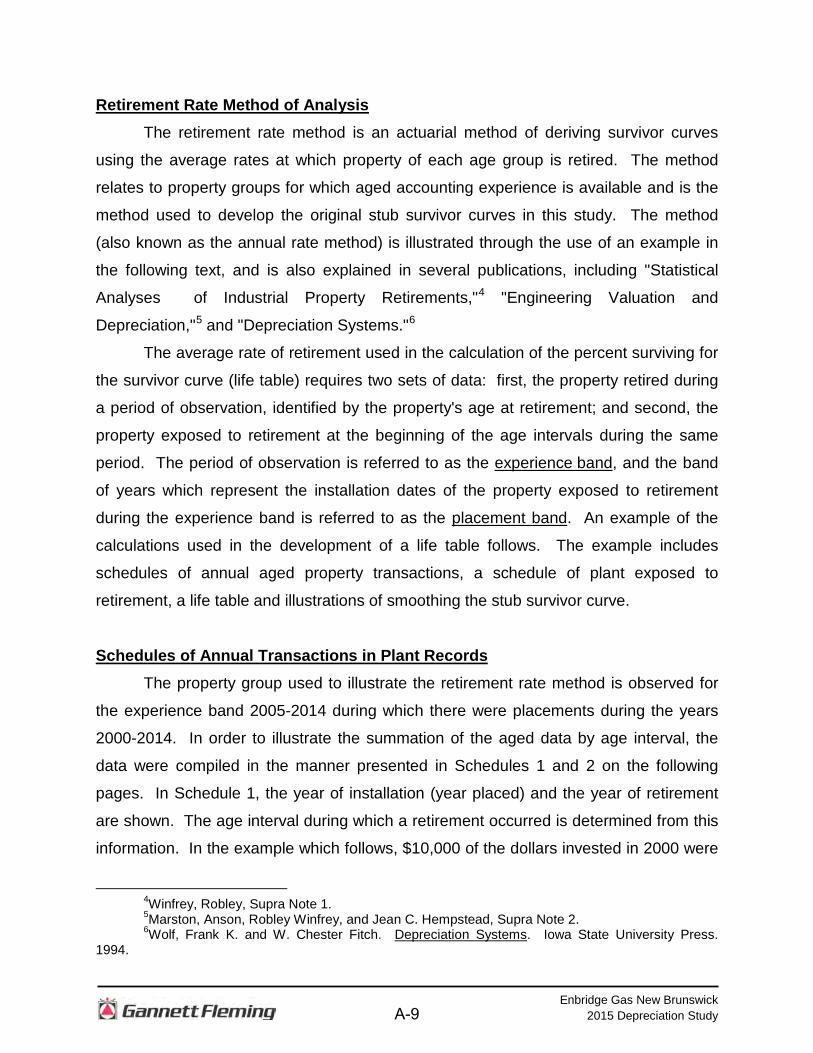
Retirement Rate Method of Analysis The retirement rate method is an actuarial method of deriving survivor curves
using the average rates at which property of each age group is retired. The method
relates to property groups for which aged accounting experience is available and is the
method used to develop the original stub survivor curves in this study. The method
(also known as the annual rate method) is illustrated through the use of an example in
the following text, and is also explained in several publications, including "Statistical
Analyses of Industrial Property Retirements,"4 "Engineering Valuation and
Depreciation,"5 and "Depreciation Systems."6 The average rate of retirement used in the calculation of the percent surviving for
the survivor curve (life table) requires two sets of data: first, the property retired during
a period of observation, identified by the property's age at retirement; and second, the
property exposed to retirement at the beginning of the age intervals during the same
period. The period of observation is referred to as the experience band, and the band
of years which represent the installation dates of the property exposed to retirement
during the experience band is referred to as the placement band. An example of the
calculations used in the development of a life table follows. The example includes
schedules of annual aged property transactions, a schedule of plant exposed to
retirement, a life table and illustrations of smoothing the stub survivor curve.
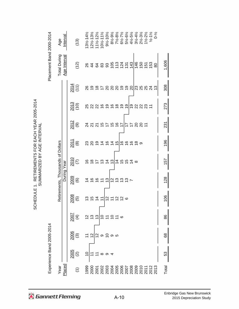
Schedules of Annual Transactions in Plant Records The property group used to illustrate the retirement rate method is observed for
the experience band 2005-2014 during which there were placements during the years
2000-2014. In order to illustrate the summation of the aged data by age interval, the
data were compiled in the manner presented in Schedules 1 and 2 on the following
pages. In Schedule 1, the year of installation (year placed) and the year of retirement
are shown. The age interval during which a retirement occurred is determined from this
information. In the example which follows, $10,000 of the dollars invested in 2000 were
4Winfrey, Robley, Supra Note 1. 5Marston, Anson, Robley Winfrey, and Jean C. Hempstead, Supra Note 2.
6Wolf, Frank K. and W. Chester Fitch. Depreciation Systems. Iowa State University Press. 1994.
A-9
Enbridge Gas New Brunswick 2015 Depreciation Study
Year
Tota
l Dur
ing
Age
Pla
ced
Age
Inte
rval
In
terv
al
2005
2006
2007
2008
2009
2010
2011
2012
2013
2014
(1)
(2)
(3)
(4)
(5)
(6)
(7)
(8)
(9)
(10)
(11)
(12)
(13)
1999
1011
1213
1416
2324
2526
2613
½-1
4½
2000
1112
1315
1618
2021
2219
4412
½-1
3½
2001
1112
1314
1617
1921
2218
6411
½-1
2½
2002
89
1011
1113
1415
1617
8310
½-1
1½
2003
910
1112
1314
1617
1920
939½
-10½
20
044
910
1112
1314
1516
2010
58½
-9½
20
055
1112
1314
1516
1820
113
7½-8
½
2006
612
1315
1617
1919
124
6½-7
½
2007
613
1516
1719
1913
15½
-6½
20
087
1416
1719
2014
34½
-5½
20
09
818
2022
2314
63½
-4½
20
109
2022
2515
02½
-3½
20
1111
2325
151
1½-2
½
2012
1124
153
½-1
½
2013
13
800-
½
Tota
l53
6886
106
128
157
196
231
273
308
1,60
6
Ret
irem
ents
, Tho
usan
ds o
f Dol
lars
D
urin
g Ye
ar
SC
HE
DU
LE 1
. R
ETI
RE
ME
NTS
FO
R E
AC
H Y
EA
R 2
005-
2014
SU
MM
AR
IZE
D B
Y A
GE
INTE
RV
AL
E
xper
ienc
e B
and
2005
-201
4P
lace
men
t Ban
d 20
00-2
014
A-10
Enbridge Gas New Brunswick 2015 Depreciation Study
E
xper
ienc
e B
and
2005
-201
4
P
lace
men
t Ban
d 20
00-2
014
Year
Tota
l Dur
ing
Age
Pla
ced
2005
2006
2007
2008
2009
2010
2011
2012
2013
2014
Age
Inte
rval
Inte
rval
(1
)(2
)(3
)(4
)(5
)(6
)(7
)(8
)(9
)(1
0)(1
1)(1
2)(1
3)
1999
--
--
--
60a
--
--
13½
-14½
2000
--
--
--
--
--
-12
½-1
3½20
01-
--
--
--
--
--
11½
-12½
2002
--
--
--
-(5
)b-
-60
10½
-11½
2003
--
--
--
-6a
--
- 9
½-1
0½20
04-
--
--
--
--
-(5
) 8
½-9
½20
05-
--
--
--
--
-7½
-8½
2006
--
--
--
--
- 6
½-7
½20
07-
--
-(1
2)b
--
- 5
½-6
½20
08-
--
-22
a-
- 4
½-5
½20
09-
-(1
9)b
--
10 3
½-4
½20
10-
--
--
2½
-3½
2011
--
(102
)c(1
21)
1½
-2½
2012
--
- ½
-1½
2013
0-½
Tota
l-
--
--
-60
(30)
22(1
02)
(50)
a T
rans
fer A
ffect
ing
Expo
sure
s at
Beg
inni
ng o
f Yea
r
b Tra
nsfe
r Affe
ctin
g Ex
posu
res
at E
nd o
f Yea
r
c Sal
e w
ith C
ontin
ued
Use
Pa
rent
hese
s D
enot
e C
redi
t Am
ount
.
Acq
uisi
tions
, Tra
nsfe
rs a
nd S
ales
, Tho
usan
ds o
f Dol
lars
Dur
ing
Year
SC
HE
DU
LE 2
. O
THE
R T
RA
NS
AC
TIO
NS
FO
R E
AC
H Y
EA
R 2
005-
2014
SU
MM
AR
IZE
D B
Y A
GE
INTE
RV
AL
A-11
Enbridge Gas New Brunswick 2015 Depreciation Study
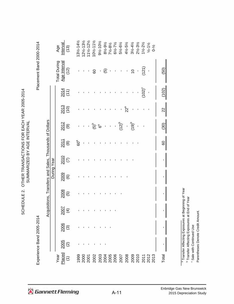
retired in 2005. The $10,000 retirement occurred during the age interval between 4½
and 5½ years on the basis that approximately one-half of the amount of property was
installed prior to and subsequent to July 1 of each year. That is, on the average,
property installed during a year is placed in service at the midpoint of the year for the
purpose of the analysis. All retirements also are stated as occurring at the midpoint of a
one-year age interval of time, except the first age interval which encompasses only one-
half year.
The total retirements occurring in each age interval in a band are determined by
summing the amounts for each transaction year-installation year combination for that
age interval. For example, the total of $143,000 retired for age interval 4½-5½ is the
sum of the retirements entered on Schedule 1 immediately above the stair step line
drawn on the table beginning with the 2005 retirements of 2000 installations and
ending with the 2014 retirements of the 2009 installations. Thus, the total amount of
143 for age interval 4½-5½ equals the sum of:
10 + 12 + 13 + 11 + 13 + 13 + 15 + 17 + 19 + 20.
In Schedule 2, other transactions which affect the group are recorded in a similar
manner. The entries illustrated include transfers and sales. The entries which are
credits to the plant account are shown in parentheses. The items recorded on this
schedule are not totaled with the retirements, but are used in developing the exposures
at the beginning of each age interval.
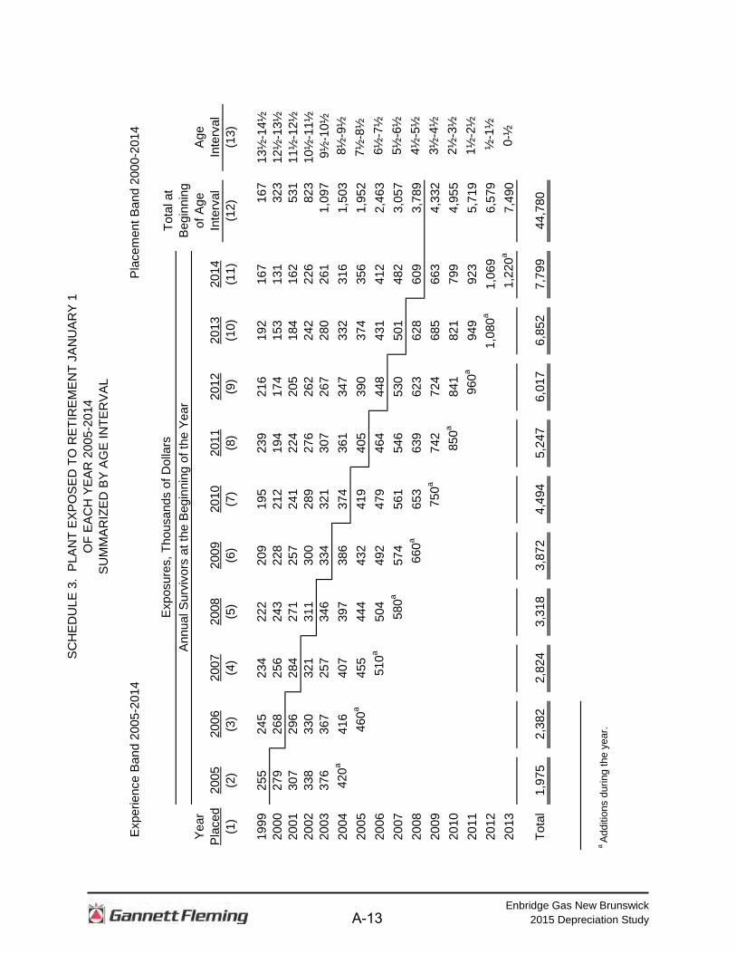
Schedule of Plant Exposed to Retirement The development of the amount of plant exposed to retirement at the beginning
of each age interval is illustrated in Schedule 3 on the following page. The surviving
plant at the beginning of each year from 2005 through 2014 is recorded by year in the
portion of the table headed "Annual Survivors at the Beginning of the Year." The last
amount entered in each column is the amount of new plant added to the group during
the year. The amounts entered in Schedule 3 for each successive year following the
beginning balance or addition, are obtained by adding or subtracting the net entries
A-12
Enbridge Gas New Brunswick 2015 Depreciation Study
E
xper
ienc
e B
and
2005
-201
4
Pla
cem
ent B
and
2000
-201
4
Tota
l at
Beg
inni
ngYe
arof
Age
Age
Pla
ced
2005
2006
2007
2008
2009
2010
2011
2012
2013
2014
Inte
rval
Inte
rval
(1)
(2)
(3)
(4)
(5)
(6)
(7)
(8)
(9)
(10)
(11)
(12)
(13)
1999
255
245
234
222
209
195
239
216
192
167
167
13½
-14½
2000
279
268
256
243
228
212
194
174
153
131
323
12½
-13½
2001
307
296
284
271
257
241
224
205
184
162
531
11½
-12½
2002
338
330
321
311
300
289
276
262
242
226
823
10½
-11½
2003
376
367
257
346
334
321
307
267
280
261
1,09
7 9
½-1
0½20
04
420
a41
640
739
738
637
436
134
733
231
61,
503
8½
-9½
2005
4
60a
455
444
432
419
405
390
374
356
1,95
27½
-8½
2006
5
10a
504
492
479
464
448
431
412
2,46
3 6
½-7
½20
07
580
a57
456
154
653
050
148
23,
057
5½
-6½
2008
6
60a
653
639
623
628
609
3,78
9 4
½-5
½20
09
750
a74
272
468
566
34,
332
3½
-4½
2010
8
50a
841
821
799
4,95
5 2
½-3
½20
11
960
a94
992
35,
719
1½
-2½
2012
1,0
80a
1,06
96,
579
½-1
½20
13 1
,220
a7,
490
0-½
Tota
l1,
975
2,38
22,
824
3,31
83,
872
4,49
45,
247
6,01
76,
852
7,79
944
,780
a Ad
ditio
ns d
urin
g th
e ye
ar.
Exp
osur
es, T
hous
ands
of D
olla
rsA
nnua
l Sur
vivo
rs a
t the
Beg
inni
ng o
f the
Yea
r
SC
HE
DU
LE 3
. P
LAN
T E
XPO
SE
D T
O R
ETI
RE
ME
NT
JAN
UA
RY
1O
F E
AC
H Y
EA
R 2
005-
2014
SU
MM
AR
IZE
D B
Y A
GE
INTE
RV
AL
A-13
Enbridge Gas New Brunswick 2015 Depreciation Study
shown on Schedules 1 and 2. For the purpose of determining the plant exposed to
retirement, transfers-in are considered as being exposed to retirement in this group at
the beginning of the year in which they occurred, and the sales and transfers-out are
considered to be removed from the plant exposed to retirement at the beginning of
the following year. Thus, the amounts of plant shown at the beginning of each year are
the amounts of plant from each placement year considered to be exposed to retirement
at the beginning of each successive transaction year. For example, the exposures for
the installation year 2006 are calculated in the following manner:
Exposures at age 0 = amount of addition = $750,000 Exposures at age ½ = $750,000 - $ 8,000 = $742,000 Exposures at age 1½ = $742,000 - $18,000 = $724,000 Exposures at age 2½ = $724,000 - $20,000 - $19,000 = $685,000 Exposures at age 3½ = $685,000 - $22,000 = $663,000
For the entire experience band 2005-2014, the total exposures at the beginning
of an age interval are obtained by summing diagonally in a manner similar to the
summing of the retirements during an age interval (Schedule 1). For example, the
figure of 3,789, shown as the total exposures at the beginning of age interval 4½-5½, is
obtained by summing: 255 + 268 + 284 + 311 + 334 + 374 + 405 + 448 + 501 + 609.
Original Life Table The original life table, illustrated in Schedule 4 on the following page, is developed from the totals shown on the schedules of retirements and exposures,
Schedules 1 and 3, respectively. The exposures at the beginning of the age interval are
obtained from the corresponding age interval of the exposure schedule, and the
retirements during the age interval are obtained from the corresponding age interval of
the retirement schedule. The retirement ratio is the result of dividing the retirements
during the age interval by the exposures at the beginning of the age interval. The
percent surviving at the beginning of each age interval is derived from survivor ratios,
each of which equals one minus the retirement ratio. The percent surviving is
developed by starting with 100% at age zero and successively multiplying the percent
A-14
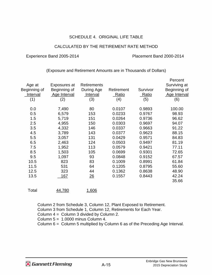
Enbridge Gas New Brunswick 2015 Depreciation Study
SCHEDULE 4. ORIGINAL LIFE TABLE
CALCULATED BY THE RETIREMENT RATE METHOD
Experience Band 2005-2014 Placement Band 2000-2014
(Exposure and Retirement Amounts are in Thousands of Dollars)
Age at
Beginning of Interval
(1)
Exposures at Beginning of Age Interval
(2)
Retirements During Age
Interval (3)
Retirement Ratio
(4)
Survivor Ratio
(5)
Percent Surviving at Beginning of Age Interval
(6)
0.0 7,490 80 0.0107 0.9893 100.00 0.5 6,579 153 0.0233 0.9767 98.93 1.5 5,719 151 0.0264 0.9736 96.62 2.5 4,955 150 0.0303 0.9697 94.07 3.5 4,332 146 0.0337 0.9663 91.22 4.5 3,789 143 0.0377 0.9623 88.15 5.5 3,057 131 0.0429 0.9571 84.83 6.5 2,463 124 0.0503 0.9497 81.19 7.5 1,952 113 0.0579 0.9421 77.11 8.5 1,503 105 0.0699 0.9301 72.65 9.5 1,097 93 0.0848 0.9152 67.57 10.5 823 83 0.1009 0.8991 61.84 11.5 531 64 0.1205 0.8795 55.60 12.5 323 44 0.1362 0.8638 48.90 13.5 167 26 0.1557 0.8443 42.24
35.66
Total
44,780
1,606
Column 2 from Schedule 3, Column 12, Plant Exposed to Retirement. Column 3 from Schedule 1, Column 12, Retirements for Each Year. Column 4 = Column 3 divided by Column 2. Column 5 = 1.0000 minus Column 4. Column 6 = Column 5 multiplied by Column 6 as of the Preceding Age Interval.
A-15
Enbridge Gas New Brunswick 2015 Depreciation Study
surviving at the beginning of each interval by the survivor ratio, i.e., one minus the
retirement ratio for that age interval. The calculations necessary to determine the
percent surviving at age 5½ are as follows:
Percent surviving at age 4½ = 88.15 Exposures at age 4½ = 3,789,000 Retirements from age 4½ to 5½ = 143,000 Retirement Ratio = 143,000 ÷ 3,789,000 = 0.0377 Survivor Ratio = 1.000 - 0.0377 = 0.9623 Percent surviving at age 5½ = (88.15) x (0.9623) = 84.83
The totals of the exposures and retirements (columns 2 and 3) are shown for the
purpose of checking with the respective totals in Schedules 1 and 3. The ratio of the
total retirements to the total exposures, other than for each age interval, is meaningless.
The original survivor curve is plotted from the original life table (column 6, Schedule 4).
When the curve terminates at a percent surviving greater than zero, it is called a stub
survivor curve. Survivor curves developed from retirement rate studies generally are
stub curves.
Smoothing the Original Survivor Curve The smoothing of the original survivor curve eliminates any irregularities and
serves as the basis for the preliminary extrapolation to zero percent surviving of the
original stub curve. Even if the original survivor curve is complete from 100% to zero
percent, it is desirable to eliminate any irregularities, as there is still an extrapolation for
the vintages which have not yet lived to the age at which the curve reaches zero
percent. In this study, the smoothing of the original curve with established type curves
was used to eliminate irregularities in the original curve.
The Iowa type curves are used in this study to smooth those original stub curves
which are expressed as percents surviving at ages in years. Each original survivor
curve was compared to the Iowa curves using visual and mathematical matching in
order to determine the better fitting smooth curves. In Figures 6, 7, and 8, the original
curve developed in Schedule 4 is compared with the L, S, and R Iowa type curves
which most nearly fit the original survivor curve. In Figure 6, the L1 curve with an
A-16
Enbridge Gas New Brunswick 2015 Depreciation Study
average life between 12 and 13 years appears to be the best fit. In Figure 7, the S0
type curve with a 12-year average life appears to be the best fit and appears to be
better than the L1 fitting. In Figure 8, the R1 type curve with a 12-year average life
appears to be the best fit and appears to be better than either the L1 or the S0.
In Figure 9, the three fittings, 12-L1, 12-S0 and 12-R1 are drawn for comparison
purposes. It is probable that the 12-R1 Iowa curve would be selected as the most
representative of the plotted survivor characteristics of the group.
A-17
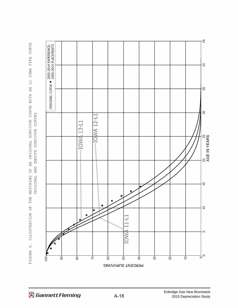
Enbridge Gas New Brunswick 2015 Depreciation Study
FIGURE 6. ILLUSTRATION OF THE MATCHING OF AN ORIGINAL SURVIVOR CURVE WITH AN L1 IOWA TYPE CURVE
ORIGINAL AND SMOOTH SURVIVOR CURVES
A-18
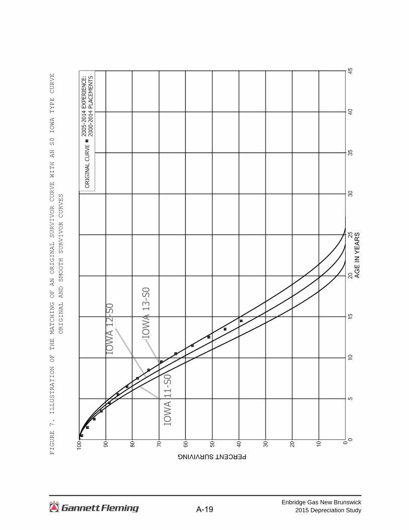
Enbridge Gas New Brunswick 2015 Depreciation Study
FIGURE 7. ILLUSTRATION OF THE MATCHING OF AN ORIGINAL SURVIVOR CURVE WITH AN S0 IOWA TYPE CURVE
ORIGINAL AND SMOOTH SURVIVOR CURVES
A-19
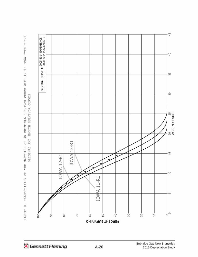
Enbridge Gas New Brunswick 2015 Depreciation Study
FIGURE 8. ILLUSTRATION OF THE MATCHING OF AN ORIGINAL SURVIVOR CURVE WITH AN R1 IOWA TYPE CURVE
ORIGINAL AND SMOOTH SURVIVOR CURVES
A-20
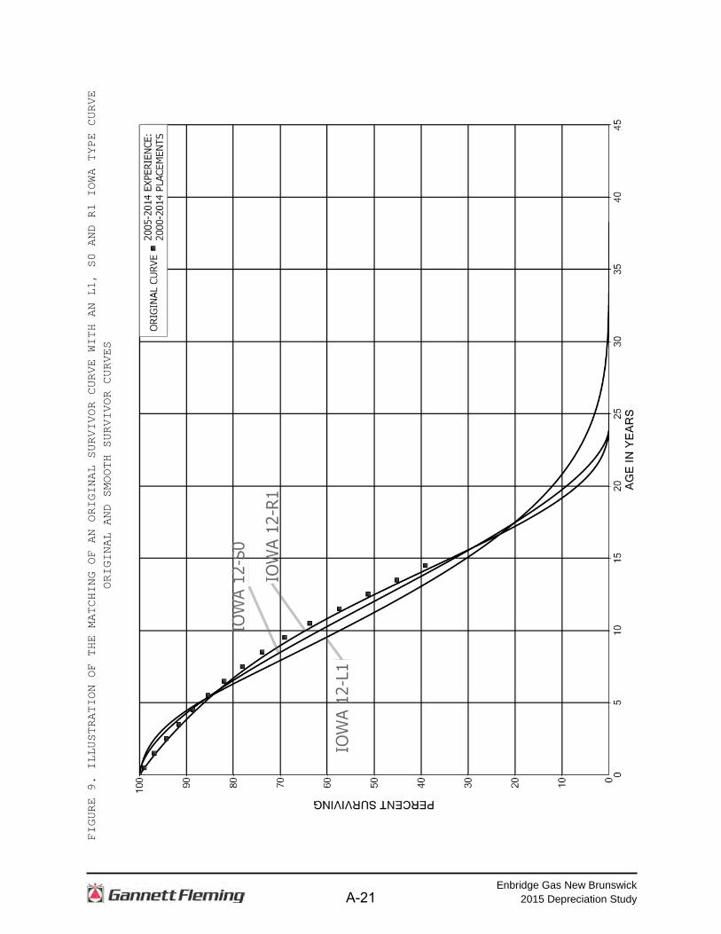
Enbridge Gas New Brunswick 2015 Depreciation Study
FIGURE 9. ILLUSTRATION OF THE MATCHING OF AN ORIGINAL SURVIVOR CURVE WITH AN L1, S0 AND R1 IOWA TYPE CURVE
ORIGINAL AND SMOOTH SURVIVOR CURVES
A-21

Gannett Fleming Canada ULC
Suite 277 • 200 Rivercrest Drive S.E. • Calgary, AB T2C 2X5 • Canada t: 403.257.5946 • f: 403.257.5947
www.gannettfleming.com