Embed Size (px)
Citation preview
Multivariate Forecast Evaluation and Rationality Testing
FEDERAL RESERVE BANK OF ST. LOUISResearch Division
P.O. Box 442St. Louis, MO 63166
RESEARCH DIVISIONWorking Paper Series
Ivana Komunjerand
Michael T. Owyang
Working Paper 2007-047D https://doi.org/10.20955/wp.2007.047
October 2011
The views expressed are those of the individual authors and do not necessarily reflect official positions of the FederalReserve Bank of St. Louis, the Federal Reserve System, or the Board of Governors.
Federal Reserve Bank of St. Louis Working Papers are preliminary materials circulated to stimulate discussion andcritical comment. References in publications to Federal Reserve Bank of St. Louis Working Papers (other than anacknowledgment that the writer has had access to unpublished material) should be cleared with the author or authors.
MULTIVARIATE FORECAST EVALUATION AND RATIONALITY
TESTING
IVANA KOMUNJER AND MICHAEL T. OWYANG
Abstract. In this paper, we propose a new family of multivariate loss func-
tions to test the rationality of vector forecasts without assuming independence
across variables. When only one variable is of interest, the loss function reduces
to the �exible asymmetric family proposed by Elliott, Komunjer and Timmer-
man (2005, 2006). Following their methodology, we derive a GMM test for
multivariate forecast rationality that allows the forecaster�s loss to be nonsep-
arable across variables, and takes into account forecast estimation uncertainty.
We use our test to study the joint rationality of macroeconomic forecasts in
the growth rate of nominal output, CPI in�ation rate, and short-term interest
rate. [JEL: C32, C53] * y
Key words and phrases. forecast rationality; multivariate loss; asymmetries
A¢liations and contact information. Komunjer: Department of Economics, University of Cal-
ifornia, San Diego [[email protected]]. Owyang: Federal Reserve Bank of St. Louis
Acknowledgments. We would like to thank the Editor, Mark Watson, as well as two anonymous
referees for their comments and suggestions that led to an improved version of the manu-
script. We bene�ted from conversations with Rick Ashley, Oscar Jorda, and Lutz Kilian.
Kristie Engemann, Charles Gascon, and Kate Vermann provided research assistance.
Disclaimer. The opinions expressed herein do not re�ect the o¢cial positions of the Federal
Reserve Bank of St. Louis or the Federal Reserve System.
MULTIVARIATE FORECASTS 1
1. Introduction
Forecasting models typically rely on the interaction of a large number of macroeconomic
variables to generate predictions. Evaluations of such forecasts, on the other hand, are largely
conducted one variable at a time (see a survey by Elliott and Timmerman, 2008). E¤ectively,
such single variable analysis imposes independence across the variables being forecast. This
means, for example, that a forecaster�s loss in output prediction errors is assumed to be
independent of her loss in in�ation prediction errors. This clearly is an undesirable feature
of any output-in�ation forecast evaluation procedure, especially if we believe that losses are
compounded by jointly overpredicting output and underpredicting in�ation; in this case,
a policymaker might be faced with unforeseen stag�ation, an outcome worse than singly
missing either prediction.
The purpose of this paper is to study the properties of vector forecasts in a framework
that does not impose independence across variables in the forecaster�s loss. Instead, we shall
assume that the forecaster�s objectives can be quanti�ed by a new family of multivariate loss
functions that are �nitely parameterized yet �exible enough to account for asymmetries in
the forecaster�s preferences as well as interactions between the variables being forecast. The
proposed family of multivariate losses permits identi�cation and estimation of the parameters
of forecasters� objectives, and allows to test for rationality of vector forecasts using over-
identifying restrictions. Similar to the scalar case, vector forecasts are said to be rational
if they are optimal under our multivariate loss; rejections of rationality should then be
interpreted as rejections of the joint hypothesis of optimality and the particular functional
form of the multivariate loss.1
MULTIVARIATE FORECASTS 2
Research on forecast rationality has a long standing history. Since the seminal works of
Muth (1961) and Lucas (1973), rationality in expectation formation has been the cornerstone
of economic models. With the availability of survey data such as the Livingston data or the
Survey of Professional Forecasters (SPF), the econometric literature on forecast evaluation
and rationality testing has seen a rapid growth (for an extensive review, see Pesaran and
Weale, 2006). Rationality is tested under a variety of assumptions on the forecasters� objec-
tives. If the latter are quadratic, then testing for rationality simply amounts to testing if the
forecast errors have zero mean, and are uncorrelated with any information available at the
time that the forecast is made. The most popular form of these tests is the Theil�Mincer�
Zarnowitz regression (see, for example, Theil, 1958; Mincer & Zanowiz, 1963; Figlewski and
Wachtel, 1981; Mishkin, 1981; Zarnowitz, 1986; Keane and Runkle, 1990).
One strand of the literature has, however, argued that asymmetric losses in which pos-
itive and negative forecast errors may be weighted di¤erently might better represent the
forecasters� objectives (see, for example, Zellner, 1986; Christo¤ersen and Diebold, 1997;
Batchelor and Peel, 1998; Elliot, Komunjer, and Timmermann, 2005; Elliot, Komunjer, and
Timmerman, 2006; Patton and Timmermann, 2007a; Patton and Timmermann, 2007b).
In particular, Elliot, Komunjer, and Timmermann (2006; EKT hereafter) and Capistran
and Timmermann (2009) �nd evidence for asymmetric loss in the SPF forecasts of output
and in�ation.2 Under asymmetric loss, forecast e¢ciency tests based on the Theil�Mincer�
Zarnowitz regressions are biased. EKT (2008) quantify the extent of the bias and its impact
on the size and power of standard rationality tests. They propose an alternative GMM based
approach that leads to correct inference regarding forecast rationality and at the same time
allows for a parsimonious parameterization of asymmetry in the forecaster�s loss.
MULTIVARIATE FORECASTS 3
An overwhelming majority of this work focuses on one variable at a time. Indeed, de-
spite the availability of vector forecasts in surveys, few studies have conducted tests in a
multivariate framework. Existing work on vector forecast rationality testing assumes that
the losses are additive separable and quadratic in individual variables�see Kirchgässner and
Müller (2006), for example. Additive separability implies that the marginal loss for one
variable (say, output) is independent of the others (say, in�ation). In other words, no in-
teractions between the variables are allowed under separability. Perhaps surprisingly, little
work has been undertaken on vector forecast evaluation that would allow for nonseparability
and asymmetries in the forecaster�s loss. This is even more striking as the decision theoretic
literature has long recognized the importance of complementarities in the utility functions
of decision makers. The main goal of this paper is to �ll this gap.
As our analysis will show, if agents have directional preferences, falsely assuming additive
separability of their objectives produces two biases: First, it can alter the results of rationality
tests. Second, it may be re�ected in a biased evaluation of the forecaster. The latter means
the econometrician may incorrectly infer a greater degree of directional preference on the
part of the forecaster. For example, if the forecaster is truly trying to forecast both output
and in�ation, then neglecting her in�ation forecast objectives when evaluating her output
forecasts may result in loss function estimates that are asymmetric, even if the forecaster�s
loss were perfecly symmetric to start with. In this paper, we argue that incorporating
nonseparable losses can, in some cases, lessen the degree of asymmetry needed to justify the
rationality of multivariate forecasts.
The practical importance of this e¤ect is signi�cant as it may help explain large degrees
of asymmetries often found in the studies of univariate forecasts. For example, EKT (2005,
MULTIVARIATE FORECASTS 4
2008) �nd that in the context of their �exible loss functions, overpredictions of output are
one and a half times costlier than underpredictions, which may be deemed implausible on
economic grounds. This paper shows that a joint evaluation of output forecasts together
with other variables such as in�ation may lead to more plausible estimates of asymmetries.
Finally, let us point out that similar to the methods developed for evaluating single variable
forecasts (EKT 2005, 2008), our forecast evaluation procedure takes into account the forecast
estimation uncertainty (see, for example, West, 1996; West 2006; West and McCraken, 1998;
McCracken, 2000; McCracken2007; Clark and McCracken, 2001; Clark and West, 2006;
Clark and West, 2007; Corradi and Swanson, 2002; Corradi and Swanson, 2006; Corradi and
Swanson 2007; Hubrich and West, 2010). Hence, we explicitly recognize the fact that the
observed forecasts typically depend on estimates of the forecasting model.
The remainder of the paper is organized as follows: Section 2 develops the theoretical
foundation for our multivariate approach. Here, we propose a new family of multivariate
loss functions and derive their properties. Where appropriate, we emphasize the di¤erences
between the separable and nonseparable losses. In Section 3 we show that the asymmetry
parameters of the proposed multivariate loss are identi�ed. Section 4 then develops the es-
timation and rationality testing procedures. In Section 5 we present a Monte Carlo example
that illustrates the properties of the proposed methods. The same section shows that mis-
specifying losses as separable leads to biased loss function estimates, and exacerbates the
degree of asymmetry needed to rationalize forecasts. Section 6 introduces the data used in
our empirical application and presents the results. Section 7 concludes. Technical details are
relegated to an Appendix. Omitted proofs and additional details can be found in an Online
Appendix.
MULTIVARIATE FORECASTS 5
2. Multivariate Forecasts and Loss Function
2.1. Setup. Hereafter, bold letters are used to denote vectors (e.g., zt) and matrices (e.g.,
B0). We consider a multivariate forecasting problem in which a forecaster is interested in
forecasting future values of an n-vector of interest yt (n > 1). Speci�cally, we let ft+s;t
denote the time-t forecast of yt+s, where s is the prediction horizon of interest, s > 1. The
forecast vector ft+s;t contains all the information comprised in the forecaster�s information
set Ft, which is informative for yt+s. We let Ft include lagged values of yt in addition to
other covariates used to predict yt+s.
For simplicity, we focus on the one-step-ahead predictions of yt+1, which we denote by
ft+1;t, knowing that all results developed in this case can readily be generalized to any
s > 1.3 Using the standard notation, we let et+1 denote the n-vector of time-t + 1 forecast
errors, et+1 = yt+1 � ft+1;t. The distribution of yt+1 conditional on Ft is denoted by F 0t (�),
F 0t (y) = P (yt+1 6 yjFt) for any y 2 Rn where 6 denotes the usual partial order on Rn. We
shall assume that:
A1. For all t = 1; 2; ::: the conditional distribution F 0t (�) is absolutely continuous with a
continuous density f 0t (�) such that f 0t (�) > 0 on Rn a.s.-P.
2.2. Multivariate Loss Function. In this paper, we generalize the �exible family of loss
functions introduced by EKT to n�variate forecasts. In the univariate case, given an expo-
nent p, 1 6 p <1, EKT map an asymmetry parameter � , �1 6 � 6 1, into a non-negative
function of a scalar error e 2 R;4 the resulting family of losses is �exible enough to accom-
modate the absolute value or quadratic losses, yet allows them to become asymmetric. We
now extend their de�nition to a vector-valued argument e 2 Rn. For this, let kukp denote
MULTIVARIATE FORECASTS 6
the lp-norm of any n-vector u = (u1; : : : ; un)0 2 Rn, i.e., kukp = (ju1jp + : : : + junjp)1=p for
1 6 p < 1, and kuk1 = max16i6n(juij); furthermore, let Bnp denote the open unit ball in
Rn, i.e., Bnp = fu 2 Rn : kukp < 1g.
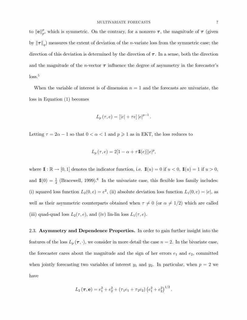
Fix a scalar p, 1 6 p < 1, and let � be an n-vector with lq-norm less than unity, i.e.,
� 2 Bnq , where 1=p+ 1=q = 1 with the convention that q =1 when p = 1. For any e 2 Rn,
we then de�ne our n-variate loss function as follows:
De�nition 1 (n-variate Loss). The n-variate loss function Lp (� ; e) : Bnq � Rn ! R, with
1 6 p <1 and 1=p+ 1=q = 1, is de�ned as
Lp (� ; e) ��kekp + � 0e
�kekp�1p : (1)
When p = 1, the multivariate loss L1(� ; e) can be used to de�ne the geometric quantiles
of the n-vector e, as proposed in Chaudhuri (1996), for example. In a sense, L1(� ; �) is a
multivariate extension of the univariate �check� (or �tick�) loss, which is well-known in the
literature on quantile estimation Koenker and Bassett (1978). When p > 1, the expression
of the n-variate loss Lp(� ; �) is entirely novel and not yet seen in the literature. We start by
establishing some of its useful properties.
Proposition 1. Let Lp(� ; e) be the n-variate loss in De�nition 1. Then, the following
properties hold: (i) Lp (� ; �) is continuous and non-negative on Rn; (ii) Lp (� ; e) = 0 if and
only if e = 0 and limkekp!1 Lp (� ; e) =1; (iii) Lp(� ; �) is convex on Rn.
A proof of Proposition 1 is in the Appendix. The shape of the n-variate loss Lp (� ; �) is
characterized by the exponent p, 1 6 p < 1. On the other hand, the n-vector � quanti�es
the extent of asymmetry in Lp (� ; �). When � = 0, the n-variate loss in Equation (1) reduces
MULTIVARIATE FORECASTS 7
to kekpp, which is symmetric. On the contrary, for a nonzero � , the magnitude of � (given
by k�kq) measures the extent of deviation of the n-variate loss from the symmetric case; the
direction of this deviation is determined by the direction of � . In a sense, both the direction
and the magnitude of the n-vector � in�uence the degree of asymmetry in the forecaster�s
loss.5
When the variable of interest is of dimension n = 1 and the forecasts are univariate, the
loss in Equation (1) becomes
Lp (� ; e) = [jej+ �e] jejp�1 :
Letting � = 2�� 1 so that 0 < � < 1 and p > 1 as in EKT, the loss reduces to
Lp (� ; e) = 2[1� � + �1I(e)]jejp;
where 1I : R! [0; 1] denotes the indicator function, i.e. 1I(u) = 0 if u < 0, 1I(u) = 1 if u > 0,
and 1I(0) = 12(Bracewell, 1999).6 In the univariate case, this �exible loss family includes:
(i) squared loss function L2(0; e) = e2, (ii) absolute deviation loss function L1(0; e) = jej, as
well as their asymmetric counterparts obtained when � 6= 0 (or � 6= 1=2) which are called
(iii) quad-quad loss L2(� ; e), and (iv) lin-lin loss L1(� ; e).
2.3. Asymmetry and Dependence Properties. In order to gain further insight into the
features of the loss Lp (� ; �), we consider in more detail the case n = 2. In the bivariate case,
the forecaster cares about the magnitude and the sign of her errors e1 and e2, committed
when jointly forecasting two variables of interest y1 and y2. In particular, when p = 2 we
have
L2 (� ; e) = e21 + e
22 + (� 1e1 + � 2e2)
�e21 + e
22
�1=2:
MULTIVARIATE FORECASTS 8
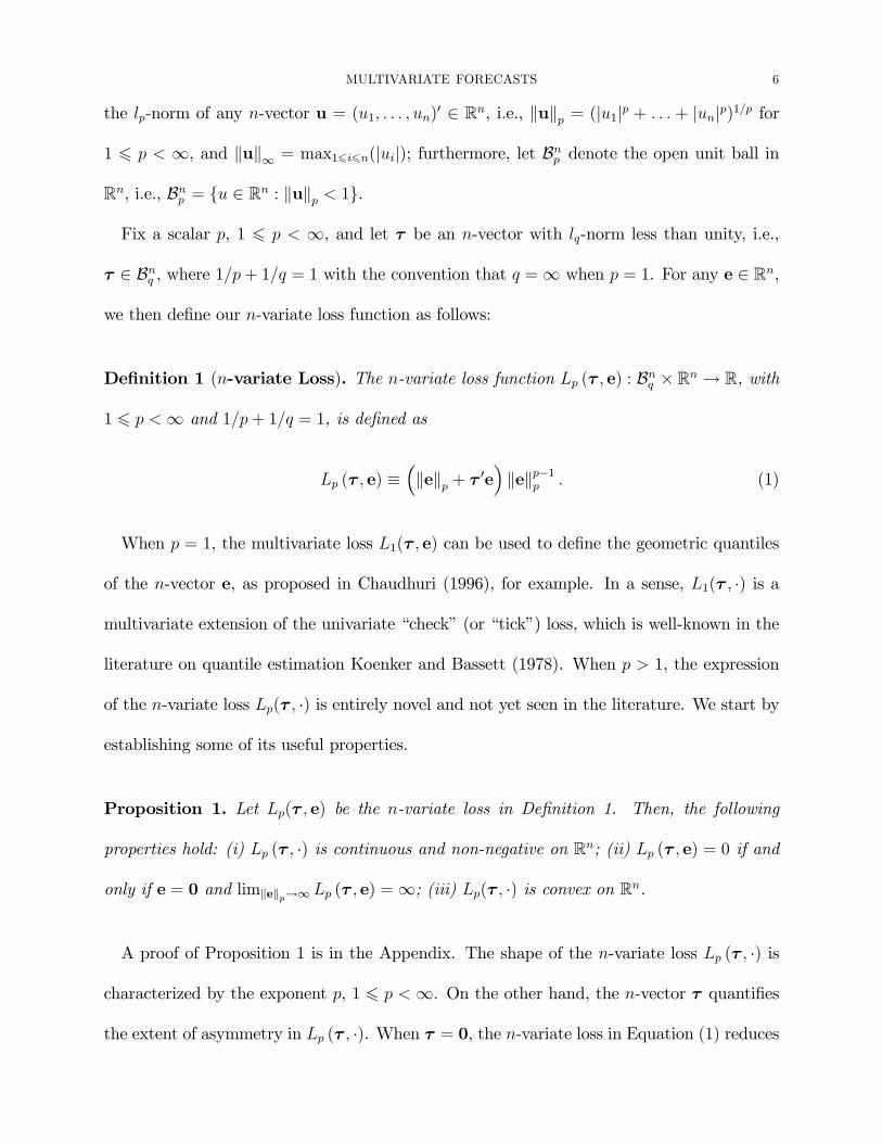
The iso-loss curves corresponding to L2 (� ; e) = constant, where e = (e1; e2)0 and � =
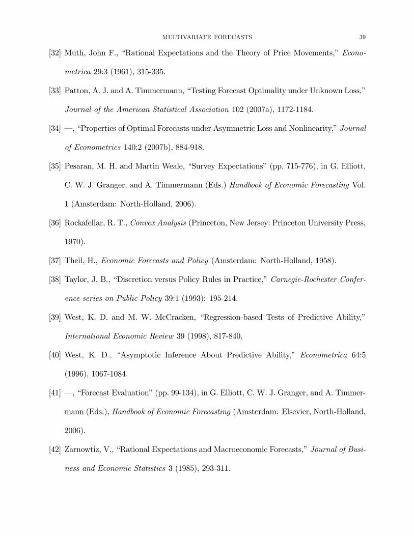
(� 1; � 2)0, are as plotted in Figure 1. Note that unless � 1 = � 2 = 0, the loss L2 (� ; e) is
nonseparable and we have
L2 (� ; e) 6= L2 (� 1; e1) + L2(� 2; e2)
for general values of the forecast errors. In other words, the bivariate loss di¤ers from a
simple sum of the individual quad-quad losses.
This property generalizes to other values of the shape parameter p as well as to higher
dimensions. If p is strictly greater than 1, then Lp (� ; e) will in general di¤er from the sum
of coordinate-wise univariate losses Lp (� 1; e1) + : : : + Lp (�n; en). Hence, minimizing the
n-variate loss Lp (� ; e) will in general produce an optimal n-vector e� whose coordinates e�i
do not necessarily each minimize Lp(� i; ei). In other words, Lp (� ; e) captures not only the
asymmetry but also the dependence between di¤erent coordinates of e.
In the special case in which the forecaster�s loss is symmetric so � = 0, the n-variate loss
becomes additively separable. That is, Lp (0; e) reduces to Lp (0; e1)+ : : :+L1(0; en) for any
value of p > 1.
3. Multivariate Forecast Rationality Condition
We now de�ne multivariate forecast rationality. Similar to the single variable case, an n-
variate forecast vector is said to be rational if it minimizes the expected value of the n-variate
loss Lp in Equation (1). Since the information sets available to the forecasters change over
time, the expectation of the loss is conditional on Ft. Hence, any rational forecast necessarily
satis�es a set of orthogonality conditions implied by the �rst-order condition of the expected
loss minimization. The key idea put forth in EKT is to use the forecast rationality condition
MULTIVARIATE FORECASTS 9
to back out the forecaster�s loss function parameters. We now extend this idea to the
multivariate case and establish global identi�ability of the asymmetry parameter � given
the shape parameter p.
Hereafter, we shall focus on the asymmetry parameter � alone; in other words, all our
results are conditional on the shape parameter p, which will be held �xed in all that follows.7
3.1. Rationality Condition. Throughout the paper, we assume that the forecaster�s n-
vector optimal forecasts of yt+1, forecasts which we denote f�t+1;t, satisfy the following ratio-
nality condition:
A2. For all t = 1; : : : we have: f�t+1;t = argminfft+1;tgE [Lp (� 0;yt+1 � ft+1;t)j Ft], where
Lp (� 0; �) is the n-variate loss function with parameter � 0 2 Bnq and 1=p+1=q = 1, 1 6 p <1
given, as de�ned in Equation (1).
When A2 holds, we say that the multivariate forecasts ff�t+1;tg are rational under the
multivariate loss Lp. Implicit in Assumption A2 are several important properties: (1) the
forecaster is an expected loss minimizer;8 (2) when constructing her optimal forecasts, the
forecaster has in mind a loss function whose argument is the forecast error n-vector et+1
alone; and (3) the forecaster�s loss is of the form Lp(� ; �) given in Equation (1) with a true
value � 0 of the asymmetry parameter � . The shape of the loss p is treated as known.
We now derive a necessary and su¢cient condition for multivariate forecast rationality,
which provides the basis of our identi�cation strategy. We need the following property:
A3. Given p, 1 6 p <1 , and for all t = 1; : : : we have:
E�kytkp�11
��Ft�<1 a.s.-P
MULTIVARIATE FORECASTS 10
and
f�t+1;t p�11
<1 a.s.-P:
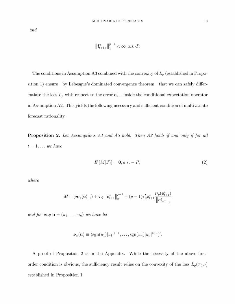
The conditions in Assumption A3 combined with the convexity of Lp (established in Propo-
sition 1) ensure�by Lebesgue�s dominated convergence theorem�that we can safely di¤er-
entiate the loss Lp with respect to the error et+1 inside the conditional expectation operator
in Assumption A2. This yields the following necessary and su¢cient condition of multivariate
forecast rationality.
Proposition 2. Let Assumptions A1 and A3 hold. Then A2 holds if and only if for all
t = 1; : : : we have
E [M jFt] = 0; a:s:� P; (2)
where
M = p�p(e�t+1) + � 0
e�t+1 p�1p
+ (p� 1)� 00e�t+1�p(e
�t+1) e�t+1 p
and for any u = (u1; : : : ; un) we have let
�p(u) � (sgn(u1)ju1jp�1; : : : ; sgn(un)junjp�1)0:
A proof of Proposition 2 is in the Appendix. While the necessity of the above �rst-
order condition is obvious, the su¢ciency result relies on the convexity of the loss Lp(� 0; �)
established in Proposition 1.
MULTIVARIATE FORECASTS 11
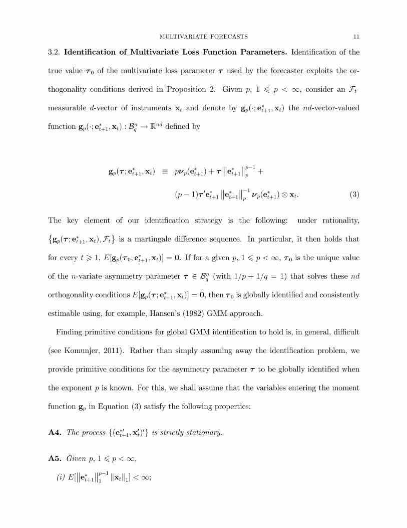
3.2. Identi�cation of Multivariate Loss Function Parameters. Identi�cation of the
true value � 0 of the multivariate loss parameter � used by the forecaster exploits the or-
thogonality conditions derived in Proposition 2. Given p, 1 6 p < 1, consider an Ft-
measurable d-vector of instruments xt and denote by gp(�; e�t+1;xt) the nd-vector-valued
function gp(�; e�t+1;xt) : Bnq ! Rnd de�ned by
gp(� ; e�t+1;xt) � p�p(e
�t+1) + �
e�t+1 p�1p
+
(p� 1)� 0e�t+1 e�t+1
�1p�p(e
�t+1) xt. (3)
The key element of our identi�cation strategy is the following: under rationality,
�gp(� ; e
�t+1;xt);Ft
is a martingale di¤erence sequence. In particular, it then holds that
for every t > 1, E[gp(� 0; e�t+1;xt)] = 0. If for a given p, 1 6 p < 1, � 0 is the unique value
of the n-variate asymmetry parameter � 2 Bnq (with 1=p + 1=q = 1) that solves these nd
orthogonality conditions E[gp(� ; e�t+1;xt)] = 0, then � 0 is globally identi�ed and consistently
estimable using, for example, Hansen�s (1982) GMM approach.
Finding primitive conditions for global GMM identi�cation to hold is, in general, di¢cult
(see Komunjer, 2011). Rather than simply assuming away the identi�cation problem, we
provide primitive conditions for the asymmetry parameter � to be globally identi�ed when
the exponent p is known. For this, we shall assume that the variables entering the moment
function gp in Equation (3) satisfy the following properties:
A4. The process f(e�0t+1;x0t)0g is strictly stationary.
A5. Given p, 1 6 p <1,
(i) E[ e�t+1
p�11kxtk1] <1;
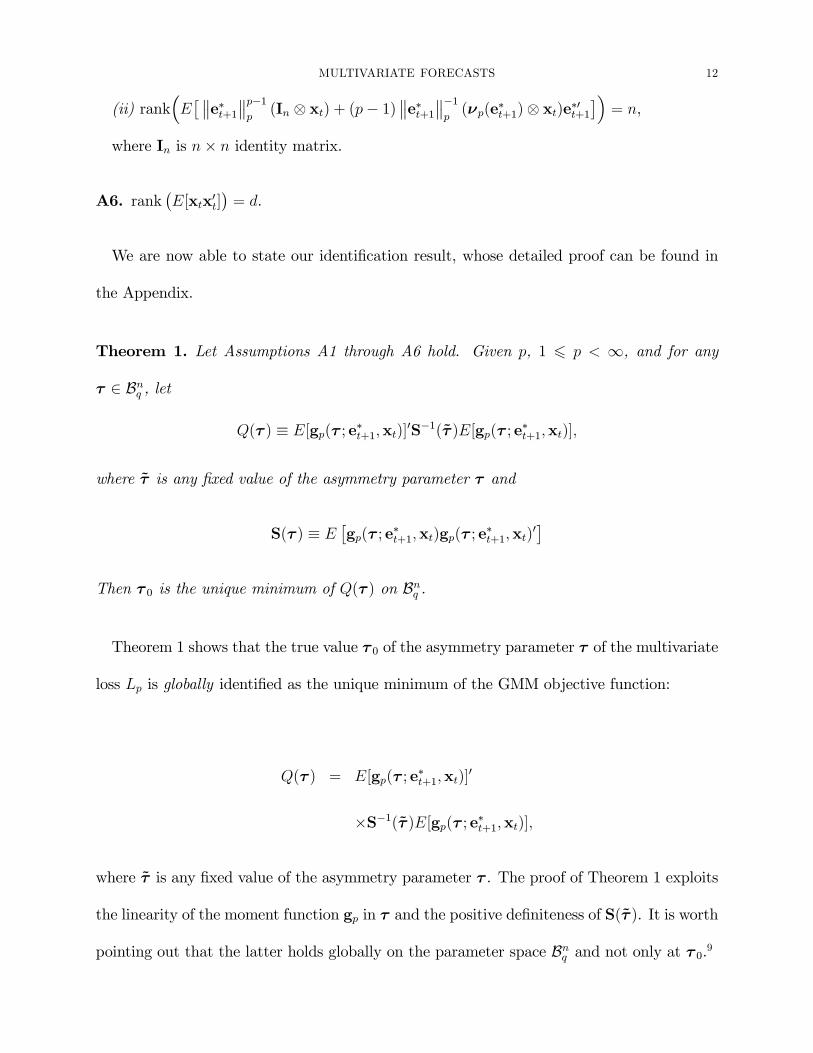
MULTIVARIATE FORECASTS 12
(ii) rank�E� e�t+1
p�1p(In xt) + (p� 1)
e�t+1 �1p(�p(e
�t+1) xt)e�0t+1
��= n,
where In is n� n identity matrix.
A6. rank�E[xtx
0t]�= d.
We are now able to state our identi�cation result, whose detailed proof can be found in
the Appendix.
Theorem 1. Let Assumptions A1 through A6 hold. Given p, 1 6 p < 1, and for any
� 2 Bnq , let
Q(� ) � E[gp(� ; e�t+1;xt)]0S�1(~� )E[gp(� ; e�t+1;xt)];
where ~� is any �xed value of the asymmetry parameter � and
S(� ) � E�gp(� ; e
�t+1;xt)gp(� ; e
�t+1;xt)
0�
Then � 0 is the unique minimum of Q(� ) on Bnq .
Theorem 1 shows that the true value � 0 of the asymmetry parameter � of the multivariate
loss Lp is globally identi�ed as the unique minimum of the GMM objective function:
Q(� ) = E[gp(� ; e�t+1;xt)]
0
�S�1(~� )E[gp(� ; e�t+1;xt)];
where ~� is any �xed value of the asymmetry parameter � . The proof of Theorem 1 exploits
the linearity of the moment function gp in � and the positive de�niteness of S(~� ). It is worth
pointing out that the latter holds globally on the parameter space Bnq and not only at � 0.9
MULTIVARIATE FORECASTS 13
4. GMM Estimation and Testing
The identi�cation result of Theorem 1 is the starting point of our estimation and multi-
variate forecast rationality testing procedures, which we now discuss.
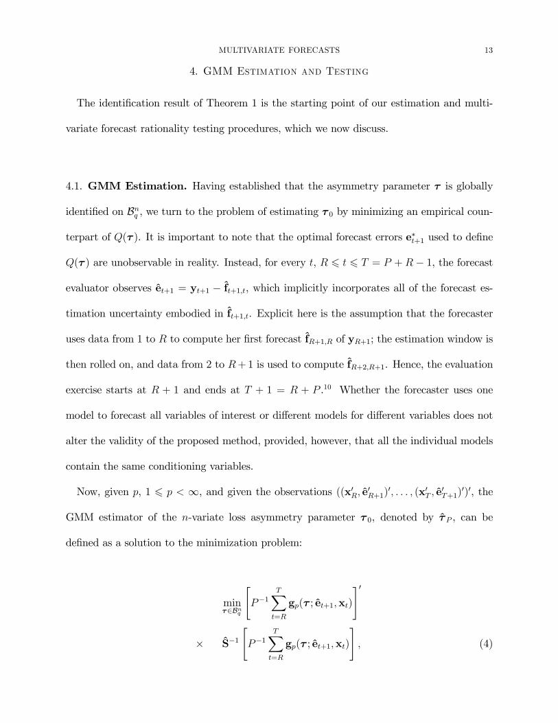
4.1. GMM Estimation. Having established that the asymmetry parameter � is globally
identi�ed on Bnq , we turn to the problem of estimating � 0 by minimizing an empirical coun-
terpart of Q(� ). It is important to note that the optimal forecast errors e�t+1 used to de�ne
Q(� ) are unobservable in reality. Instead, for every t, R 6 t 6 T = P + R� 1, the forecast
evaluator observes et+1 = yt+1 � ft+1;t, which implicitly incorporates all of the forecast es-
timation uncertainty embodied in ft+1;t. Explicit here is the assumption that the forecaster
uses data from 1 to R to compute her �rst forecast fR+1;R of yR+1; the estimation window is
then rolled on, and data from 2 to R+1 is used to compute fR+2;R+1. Hence, the evaluation
exercise starts at R + 1 and ends at T + 1 = R + P .10 Whether the forecaster uses one
model to forecast all variables of interest or di¤erent models for di¤erent variables does not
alter the validity of the proposed method, provided, however, that all the individual models
contain the same conditioning variables.
Now, given p, 1 6 p < 1, and given the observations ((x0R; e0R+1)0; : : : ; (x0T ; e0T+1)0)0, the
GMM estimator of the n-variate loss asymmetry parameter � 0, denoted by �P , can be
de�ned as a solution to the minimization problem:
min�2Bnq
"P�1
TX
t=R
gp(� ; et+1;xt)
#0
� S�1
"P�1
TX
t=R
gp(� ; et+1;xt)
#; (4)
MULTIVARIATE FORECASTS 14
where S is a consistent estimator of
S = E[gp(� 0; e�t+1;xt)gp(� 0; e
�t+1;xt)
0]:
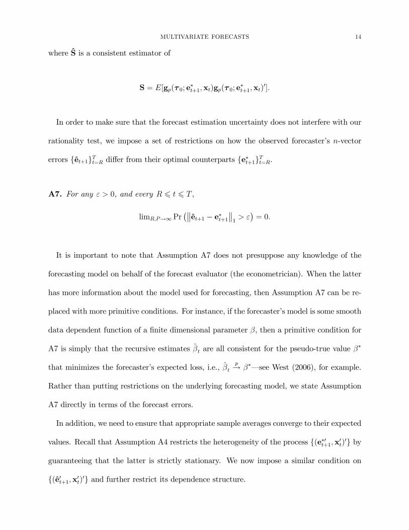
In order to make sure that the forecast estimation uncertainty does not interfere with our
rationality test, we impose a set of restrictions on how the observed forecaster�s n-vector
errors fet+1gTt=R di¤er from their optimal counterparts fe�t+1gTt=R.
A7. For any " > 0, and every R 6 t 6 T ,
limR;P!1 Pr� et+1 � e�t+1
1> "�= 0:
It is important to note that Assumption A7 does not presuppose any knowledge of the
forecasting model on behalf of the forecast evaluator (the econometrician). When the latter
has more information about the model used for forecasting, then Assumption A7 can be re-
placed with more primitive conditions. For instance, if the forecaster�s model is some smooth
data dependent function of a �nite dimensional parameter �, then a primitive condition for
A7 is simply that the recursive estimates �t are all consistent for the pseudo-true value ��
that minimizes the forecaster�s expected loss, i.e., �tp! ���see West (2006), for example.
Rather than putting restrictions on the underlying forecasting model, we state Assumption
A7 directly in terms of the forecast errors.
In addition, we need to ensure that appropriate sample averages converge to their expected
values. Recall that Assumption A4 restricts the heterogeneity of the process f(e�0t+1;x0t)0g by
guaranteeing that the latter is strictly stationary. We now impose a similar condition on
f(e0t+1;x0t)0g and further restrict its dependence structure.
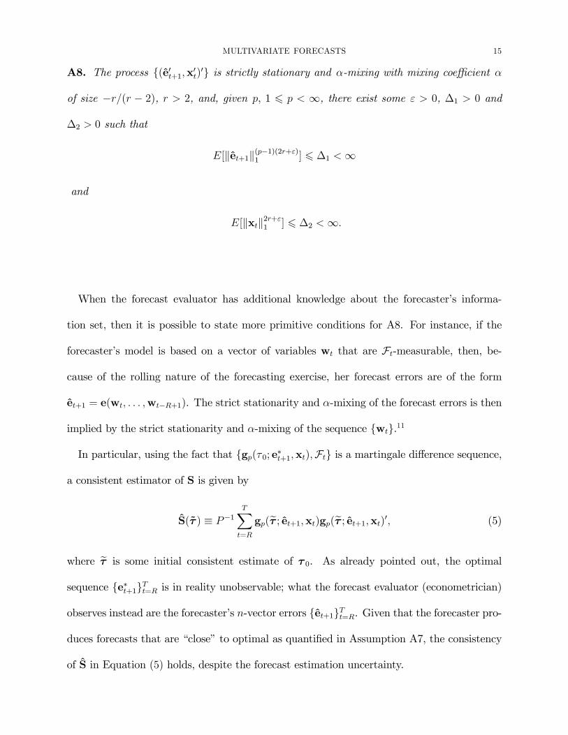
MULTIVARIATE FORECASTS 15
A8. The process f(e0t+1;x0t)0g is strictly stationary and �-mixing with mixing coe¢cient �
of size �r=(r � 2), r > 2, and, given p, 1 6 p < 1, there exist some " > 0, �1 > 0 and
�2 > 0 such that
E[ket+1k(p�1)(2r+")1 ] 6 �1 <1
and
E[kxtk2r+"1 ] 6 �2 <1:
When the forecast evaluator has additional knowledge about the forecaster�s informa-
tion set, then it is possible to state more primitive conditions for A8. For instance, if the
forecaster�s model is based on a vector of variables wt that are Ft-measurable, then, be-
cause of the rolling nature of the forecasting exercise, her forecast errors are of the form
et+1 = e(wt; : : : ;wt�R+1). The strict stationarity and �-mixing of the forecast errors is then
implied by the strict stationarity and �-mixing of the sequence fwtg.11
In particular, using the fact that fgp(� 0; e�t+1;xt);Ftg is a martingale di¤erence sequence,
a consistent estimator of S is given by
S(~� ) � P�1TX
t=R
gp(e� ; et+1;xt)gp(e� ; et+1;xt)0; (5)
where e� is some initial consistent estimate of � 0. As already pointed out, the optimal
sequence fe�t+1gTt=R is in reality unobservable; what the forecast evaluator (econometrician)
observes instead are the forecaster�s n-vector errors fet+1gTt=R. Given that the forecaster pro-
duces forecasts that are �close� to optimal as quanti�ed in Assumption A7, the consistency
of S in Equation (5) holds, despite the forecast estimation uncertainty.
MULTIVARIATE FORECASTS 16
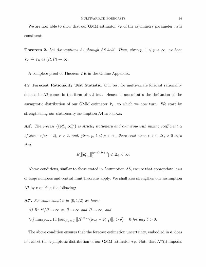
We are now able to show that our GMM estimator �P of the asymmetry parameter � 0 is
consistent:
Theorem 2. Let Assumptions A1 through A8 hold. Then, given p, 1 6 p < 1, we have
�Pp! � 0 as (R;P )!1.
A complete proof of Theorem 2 is in the Online Appendix.
4.2. Forecast Rationality Test Statistic. Our test for multivariate forecast rationality
de�ned in A2 comes in the form of a J-test. Hence, it necessitates the derivation of the
asymptotic distribution of our GMM estimator �P , to which we now turn. We start by
strengthening our stationarity assumption A4 as follows:
A40. The process f(e�0t+1;x0t)0g is strictly stationary and �-mixing with mixing coe¢cient �
of size �r=(r � 2), r > 2, and, given p, 1 6 p < 1, there exist some � > 0, �3 > 0 such
that
E[ e�t+1
(p�1)(2r+�)1
] 6 �3 <1:
Above conditions, similar to those stated in Assumption A8, ensure that appropriate laws
of large numbers and central limit theorems apply. We shall also strengthen our assumption
A7 by requiring the following:
A70. For some small " in (0; 1=2) we have:
(i) R1�2"=P !1 as R!1 and P !1, and
(ii) limR;P!1 Pr�supR6t6T
R1=2�"(et+1 � e�t+1) 1> ��= 0 for any � > 0.
The above condition ensures that the forecast estimation uncertainty, embodied in e, does
not a¤ect the asymptotic distribution of our GMM estimator �P . Note that A70(i) imposes
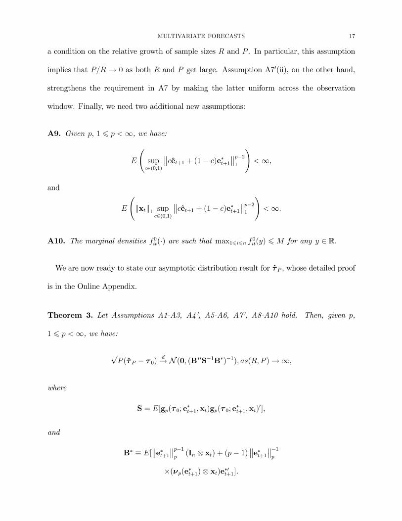
MULTIVARIATE FORECASTS 17
a condition on the relative growth of sample sizes R and P . In particular, this assumption
implies that P=R ! 0 as both R and P get large. Assumption A70(ii), on the other hand,
strengthens the requirement in A7 by making the latter uniform across the observation
window. Finally, we need two additional new assumptions:
A9. Given p, 1 6 p <1, we have:
E
supc2(0;1)
cet+1 + (1� c)e�t+1 p�21
!<1;
and
E
kxtk1 sup
c2(0;1)
cet+1 + (1� c)e�t+1 p�21
!<1:
A10. The marginal densities f 0it(�) are such that max16i6n f 0it(y) 6M for any y 2 R.
We are now ready to state our asymptotic distribution result for �P , whose detailed proof
is in the Online Appendix.
Theorem 3. Let Assumptions A1-A3, A4�, A5-A6, A7�, A8-A10 hold. Then, given p,
1 6 p <1, we have:
pP (�P � � 0) d! N (0; (B�0S�1B�)�1); as(R;P )!1;
where
S = E[gp(� 0; e�t+1;xt)gp(� 0; e
�t+1;xt)
0];
and
B� � E[ e�t+1
p�1p(In xt) + (p� 1)
e�t+1 �1p
�(�p(e�t+1) xt)e�0t+1].
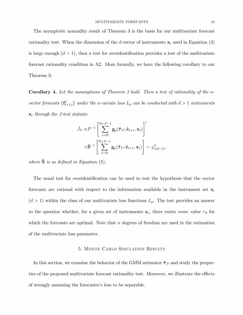
MULTIVARIATE FORECASTS 18
The asymptotic normality result of Theorem 3 is the basis for our multivariate forecast
rationality test. When the dimension of the d-vector of instruments xt used in Equation (3)
is large enough (d > 1), then a test for overidenti�cation provides a test of the multivariate
forecast rationality condition in A2. More formally, we have the following corollary to our
Theorem 3:
Corollary 4. Let the assumptions of Theorem 3 hold. Then a test of rationality of the n-
vector forecasts ff�t+1;tg under the n-variate loss Lp can be conducted with d > 1 instruments
xt through the J-test statistic
JP �P�1"R+P�1X
t=R
gp(�P ; et+1;xt)
#0
�S�1"R+P�1X
t=R
gp(�P ; et+1;xt)
#� �2n(d�1);
where S is as de�ned in Equation (5).
The usual test for overidenti�cation can be used to test the hypothesis that the vector
forecasts are rational with respect to the information available in the instrument set xt
(d > 1) within the class of our multivariate loss functions Lp. The test provides an answer
to the question whether, for a given set of instruments xt, there exists some value � 0 for
which the forecasts are optimal. Note that n degrees of freedom are used in the estimation
of the multivariate loss parameter.
5. Monte Carlo Simulation Results
In this section, we examine the behavior of the GMM estimator �P and study the proper-
ties of the proposed multivariate forecast rationality test. Moreover, we illustrate the e¤ects
of wrongly assuming the forecaster�s loss to be separable.
MULTIVARIATE FORECASTS 19
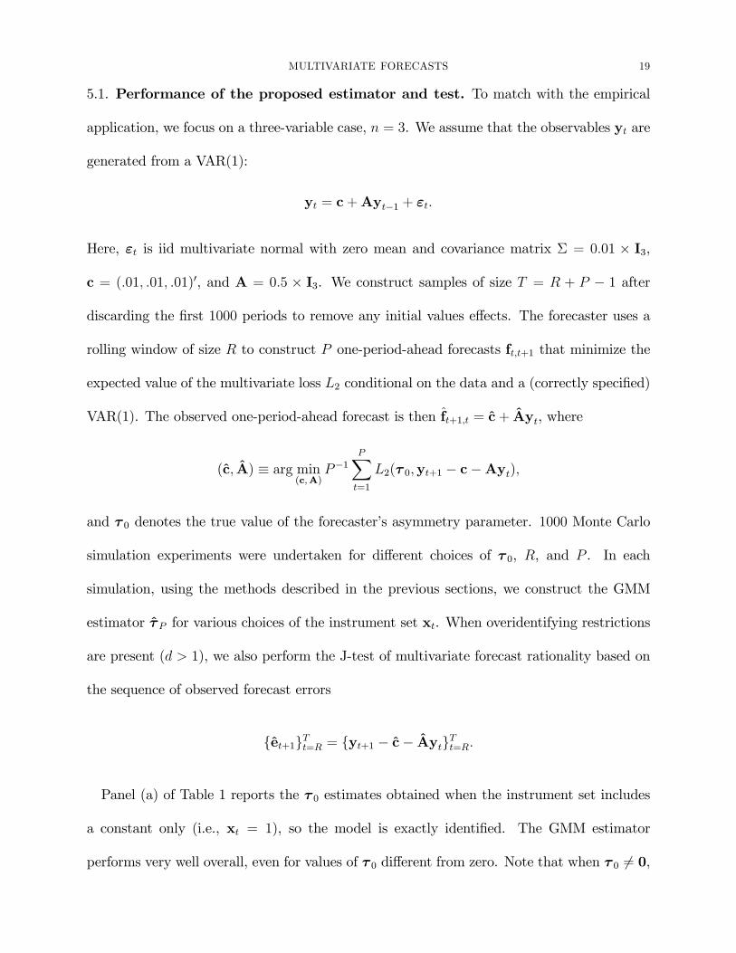
5.1. Performance of the proposed estimator and test. To match with the empirical
application, we focus on a three-variable case, n = 3. We assume that the observables yt are
generated from a VAR(1):
yt = c+Ayt�1 + "t:
Here, "t is iid multivariate normal with zero mean and covariance matrix � = 0:01 � I3,
c = (:01; :01; :01)0, and A = 0:5 � I3. We construct samples of size T = R + P � 1 after
discarding the �rst 1000 periods to remove any initial values e¤ects. The forecaster uses a
rolling window of size R to construct P one-period-ahead forecasts ft;t+1 that minimize the
expected value of the multivariate loss L2 conditional on the data and a (correctly speci�ed)
VAR(1). The observed one-period-ahead forecast is then ft+1;t = c+ Ayt, where
(c; A) � arg min(c;A)
P�1PX
t=1
L2(� 0;yt+1 � c�Ayt);
and � 0 denotes the true value of the forecaster�s asymmetry parameter. 1000 Monte Carlo
simulation experiments were undertaken for di¤erent choices of � 0, R, and P . In each
simulation, using the methods described in the previous sections, we construct the GMM
estimator �P for various choices of the instrument set xt. When overidentifying restrictions
are present (d > 1), we also perform the J-test of multivariate forecast rationality based on
the sequence of observed forecast errors
fet+1gTt=R = fyt+1 � c� AytgTt=R:
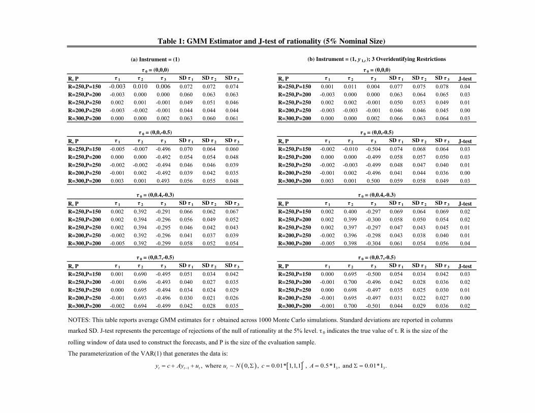
Panel (a) of Table 1 reports the � 0 estimates obtained when the instrument set includes
a constant only (i.e., xt = 1), so the model is exactly identi�ed. The GMM estimator
performs very well overall, even for values of � 0 di¤erent from zero. Note that when � 0 6= 0,
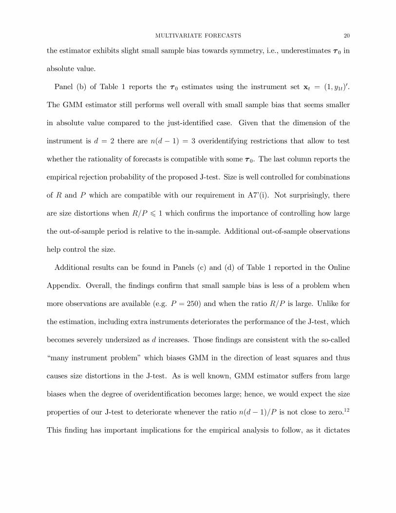
MULTIVARIATE FORECASTS 20
the estimator exhibits slight small sample bias towards symmetry, i.e., underestimates � 0 in
absolute value.
Panel (b) of Table 1 reports the � 0 estimates using the instrument set xt = (1; y1t)0.
The GMM estimator still performs well overall with small sample bias that seems smaller
in absolute value compared to the just-identi�ed case. Given that the dimension of the
instrument is d = 2 there are n(d � 1) = 3 overidentifying restrictions that allow to test
whether the rationality of forecasts is compatible with some � 0. The last column reports the
empirical rejection probability of the proposed J-test. Size is well controlled for combinations
of R and P which are compatible with our requirement in A7�(i). Not surprisingly, there
are size distortions when R=P 6 1 which con�rms the importance of controlling how large
the out-of-sample period is relative to the in-sample. Additional out-of-sample observations
help control the size.
Additional results can be found in Panels (c) and (d) of Table 1 reported in the Online
Appendix. Overall, the �ndings con�rm that small sample bias is less of a problem when
more observations are available (e.g. P = 250) and when the ratio R=P is large. Unlike for
the estimation, including extra instruments deteriorates the performance of the J-test, which
becomes severely undersized as d increases. Those �ndings are consistent with the so-called
�many instrument problem� which biases GMM in the direction of least squares and thus
causes size distortions in the J-test. As is well known, GMM estimator su¤ers from large
biases when the degree of overidenti�cation becomes large; hence, we would expect the size
properties of our J-test to deteriorate whenever the ratio n(d � 1)=P is not close to zero.12
This �nding has important implications for the empirical analysis to follow, as it dictates
MULTIVARIATE FORECASTS 21
the maximum number of instruments one can safely use with sample sizes around P = 150,
which will be the case here.
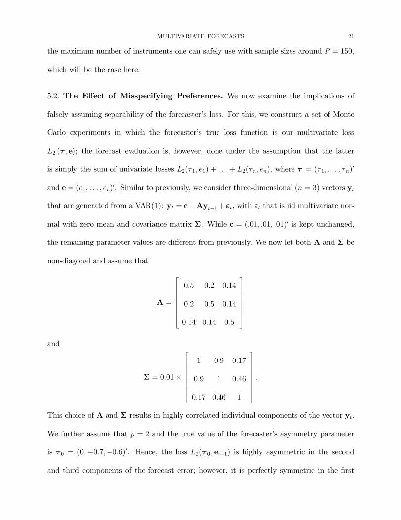
5.2. The E¤ect of Misspecifying Preferences. We now examine the implications of
falsely assuming separability of the forecaster�s loss. For this, we construct a set of Monte
Carlo experiments in which the forecaster�s true loss function is our multivariate loss
L2 (� ; e); the forecast evaluation is, however, done under the assumption that the latter
is simply the sum of univariate losses L2(� 1; e1) + : : : + L2(�n; en), where � = (� 1; : : : ; �n)0
and e = (e1; : : : ; en)0. Similar to previously, we consider three-dimensional (n = 3) vectors yt
that are generated from a VAR(1): yt = c+Ayt�1+ "t, with "t that is iid multivariate nor-
mal with zero mean and covariance matrix �. While c = (:01; :01; :01)0 is kept unchanged,
the remaining parameter values are di¤erent from previously. We now let both A and � be
non-diagonal and assume that
A =
2666664
0:5 0:2 0:14
0:2 0:5 0:14
0:14 0:14 0:5
3777775
and
� = 0:01�
2666664
1 0:9 0:17
0:9 1 0:46
0:17 0:46 1
3777775:
This choice of A and � results in highly correlated individual components of the vector yt.
We further assume that p = 2 and the true value of the forecaster�s asymmetry parameter
is � 0 = (0;�0:7;�0:6)0. Hence, the loss L2(� 0; et+1) is highly asymmetric in the second
and third components of the forecast error; however, it is perfectly symmetric in the �rst
MULTIVARIATE FORECASTS 22
component. As previously, we use a rolling window of size R = 250 to construct P = 150
one-period-ahead forecasts.
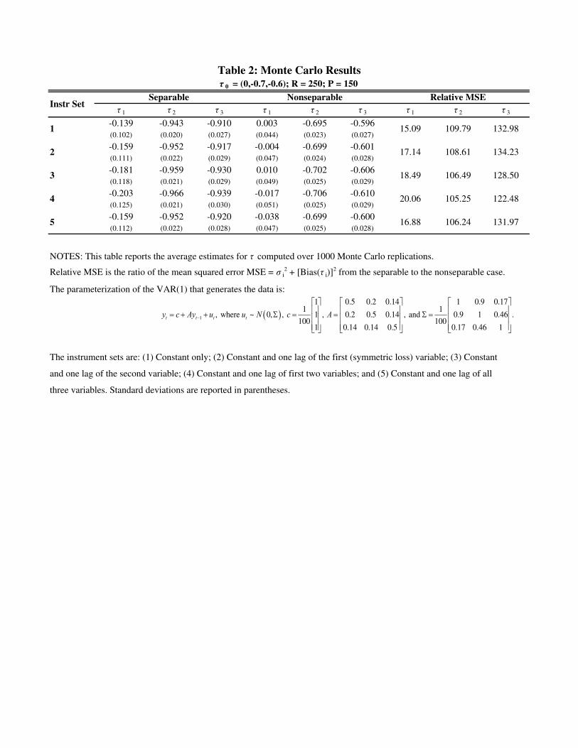
Table 2 presents the results from 1000 Monte Carlo replications of the above parameter-
ization using �ve information sets. The e¤ects of misspecifying the loss as separable when
the forecaster has asymmetric preferences and the variables are correlated become evident.
Under separable loss, the forecaster appears to have asymmetric preferences for the �rst
variable (with � 1 ranging from �0:14 to �0:20 according to the choice of instruments) even
though her true preferences are symmetric with � 01 = 0. For the two other variables, mis-
speci�cation results in more asymmetric estimates for � 02 = �0:7 and � 03 = �0:6, with � 2
and � 3 ranging from �0:91 to �0:97 across information sets.
These �ndings have important implications on the interpretation of the univariate ratio-
nality test results. For example, consider the �ndings of EKT (2008) obtained when testing
the rationality of SPF forecasts for GDP growth. Using their �exible univariate loss speci�-
cation, EKT (2008) �nd the individual � estimates consistent with rationality to be clustered
around 0:4. Translated into our setup, this would correspond to � estimates clustered around
�0:2. From this evidence, EKT (2008) conclude (p.141) that �asymmetry in the loss func-
tion is required to overturn rejections of the null hypothesis [that GDP growth forecasts are
rational].� Our Monte Carlo experiment o¤ers an alternative interpretation of this �nding:
the forecasters� losses are perfectly symmetric in their GDP forecast errors; however, those
errors are not independent of the forecast errors committed in other variables.
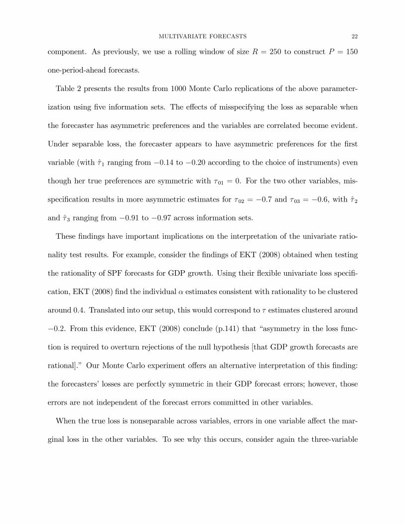
When the true loss is nonseparable across variables, errors in one variable a¤ect the mar-
ginal loss in the other variables. To see why this occurs, consider again the three-variable
MULTIVARIATE FORECASTS 23
case:
L2 (� ; e) = e21 + e22 + e
23 +
(� 1e1 + � 2e2 + � 3e3)�e21 + e
22 + e
23
�1=2:
Then,
@L2 (� ; e)
@e1= 2e1 + � 1
�e21 + e
22 + e
23
�1=2+
(� 1e1 + � 2e2 + � 3e3)e1
(e21 + e22 + e
23)1=2:
Thus, even if � 1 = 0 (i.e., the forecaster�s preferences are symmetric over the �rst variable),
the marginal loss in the �rst variable @L2 (� ; e) =@e1 depends on the remaining errors (e2; e3).
Wrongly assuming separability (i.e., that @L2 (� ; e) =@e1 is a function of e1 alone) then results
in biased estimates of � .
6. Empirical Application
We illustrate the performance of our procedure in a situation in which three macroeco-
nomic variables are jointly forecast: growth rate in output (y), CPI in�ation rate (�), and
short-term interest rate (r). Examples of models using these variables include Taylor�s (1993)
interest rate targeting rule, monetary VARs (Christiano, Eichenbaum, and Evens,k 1999),
optimizing ISLM models (McCallum and Nelson, 1999), and reduced-form New Keynesian
models (Clarida, Galì, and Gertler, 2000). Common to these models is a relationship�
either estimated or imposed�between output and prices combined with the Federal Re-
serve�s control of short-term interest rates. We would thus expect the forecaster�s loss to be
nonseparable across variables.
MULTIVARIATE FORECASTS 24
6.1. Data. Forecast data are taken from the Blue Chip Economic Indicators (BCEI), a com-
pilation of industry forecasts of a number of economic variables. Each month, participating
�rms report forecasts of the current- or next-year growth rate in output and prices and the
current- or next-year average short-term interest rate. Our sample includes forecasts from
1976:08 to 2004:12.
We assume that the forecaster�s objective is to predict true values and that revisions to
the realizations are a more accurate re�ection of the true values. Thus, in constructing the
forecast errors, we use the latest revision of the variable in question. The realizations are
yearly growth rates of GDP, GNP, and CPI in�ation. Short-term interest rate realizations
are the yearly averages.
Over time, some forecasters leave the sample while others are added. In addition, �rms
occasionally fail to report forecasts for any given month. We therefore omit any observation
in which forecasts for all three variables are not reported. These observations may a¤ect
both the period in which the forecast is made and the information set of the forecaster.
In these cases, both observations are omitted. Finally, forecasters with fewer than 80 valid
observations are dropped from the sample. This leaves 57 �rms with an average of 171 valid
observations per �rm.
The set of instruments xt used in the implementation of our procedure includes combi-
nations of the lagged growth rates of output, in�ation, the unemployment rate, and the
short-term interest rate. Instruments are, for each month, a snapshot of the real-time data
available at that time.13 The instrument sets are de�ned in Table 3. As a baseline for com-
parison, we repeat each test under the assumption of separability and the joint assumption
of separability and symmetry.
MULTIVARIATE FORECASTS 25
6.2. Multivariate Rationality Test Results. Table 4 illustrates the e¤ect of testing ra-
tionality using the nonseparable loss L2(� ; e), separable loss
L2(� 1; e1) + L2(� 2; e2) + L2(� 3; e3);
as well as separable symmetric loss
L2(0; e1) + L2(0; e2) + L2(0; e3):
We report the percentages of forecasters for which rationality could be rejected at the 10%,
5% and 1% levels, for each set of instruments. p = 2 is kept �xed in all con�gurations. For
any instrument set, both asymmetric loss functions reject rationality for a lower percentage
of forecasters than the separable symmetric baseline. The percentage of forecasters for which
rationality is rejected under nonseparable loss is relatively close to that under separable loss.
Rationality under separable symmetric loss is, however, overwhelmingly rejected. Interest-
ingly, the smallest percentage of forecasters are found to be rational with respect to the
unemployment rate (information set 5).
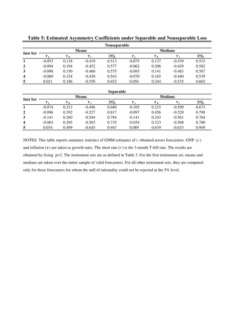
6.3. Asymmetry Coe¢cients. For a given speci�cation of the forecaster�s loss function,
our procedure delivers estimates of the asymmetry parameters (� y; ��; � r) most consistent
with the orthogonality conditions implied by rationality of joint forecasts of y, �, and r.
EKT found that the addition of asymmetric loss alone can increase the percentage of fore-
casters for which rationality is con�rmed. However, for the separable loss functions implied
by EKT, this �nding often requires substantial directional asymmetry in the forecasters� loss
functions. Allowing the forecaster�s marginal loss to depend on all of the variables being
forecast may ameliorate this problem. Recall that interpretation of the asymmetry parame-
ters (� y; ��; � r) depends on their values relative to the baseline 0. Values greater (less) than
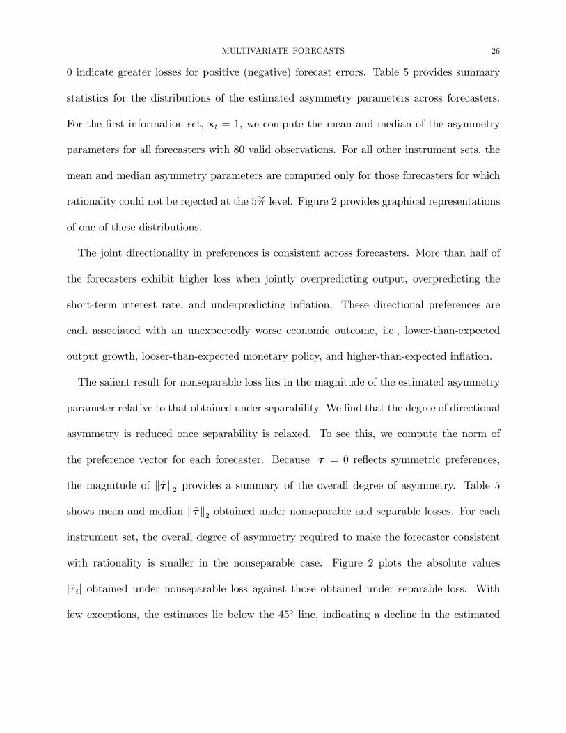
MULTIVARIATE FORECASTS 26
0 indicate greater losses for positive (negative) forecast errors. Table 5 provides summary
statistics for the distributions of the estimated asymmetry parameters across forecasters.
For the �rst information set, xt = 1, we compute the mean and median of the asymmetry
parameters for all forecasters with 80 valid observations. For all other instrument sets, the
mean and median asymmetry parameters are computed only for those forecasters for which
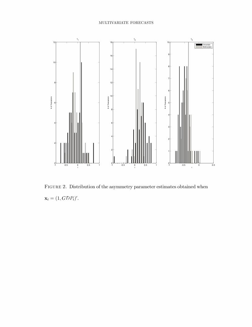
rationality could not be rejected at the 5% level. Figure 2 provides graphical representations
of one of these distributions.
The joint directionality in preferences is consistent across forecasters. More than half of
the forecasters exhibit higher loss when jointly overpredicting output, overpredicting the
short-term interest rate, and underpredicting in�ation. These directional preferences are
each associated with an unexpectedly worse economic outcome, i.e., lower-than-expected
output growth, looser-than-expected monetary policy, and higher-than-expected in�ation.
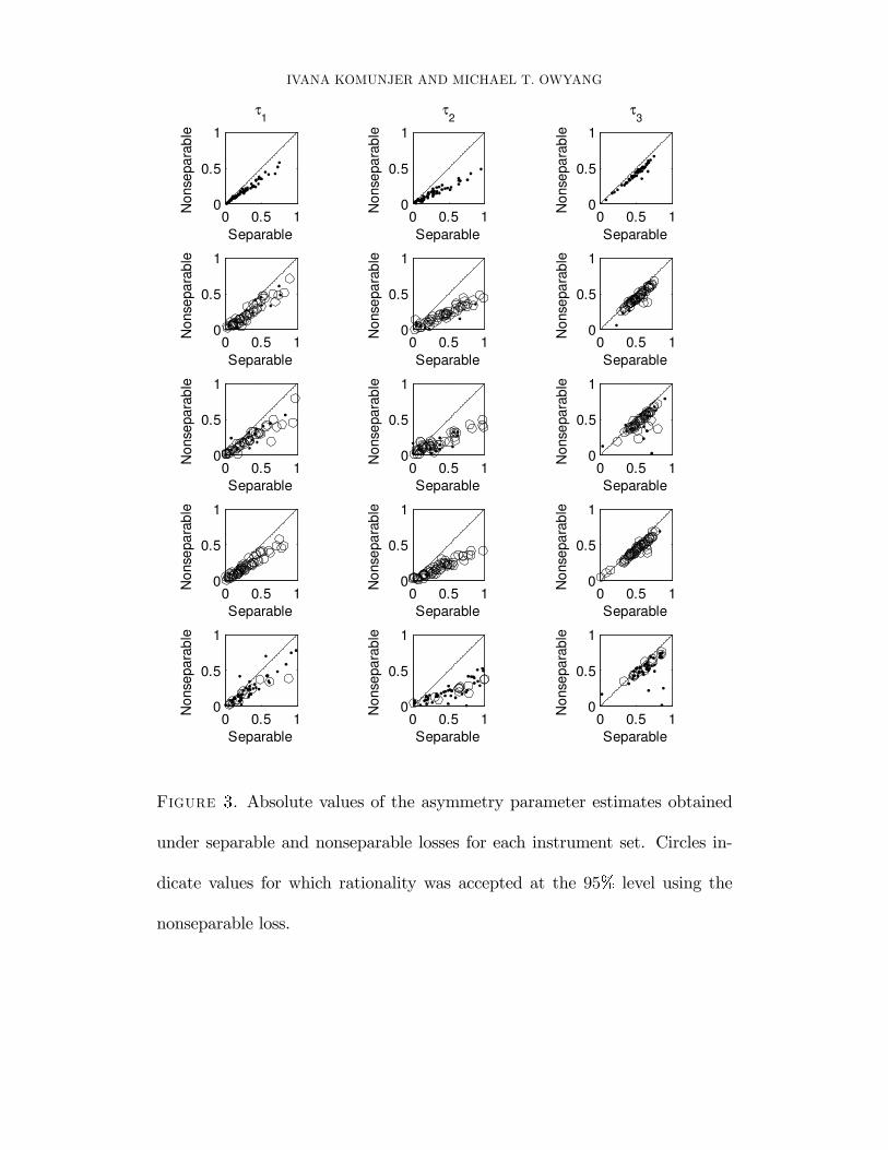
The salient result for nonseparable loss lies in the magnitude of the estimated asymmetry
parameter relative to that obtained under separability. We �nd that the degree of directional
asymmetry is reduced once separability is relaxed. To see this, we compute the norm of
the preference vector for each forecaster. Because � = 0 re�ects symmetric preferences,
the magnitude of k�k2 provides a summary of the overall degree of asymmetry. Table 5
shows mean and median k�k2 obtained under nonseparable and separable losses. For each
instrument set, the overall degree of asymmetry required to make the forecaster consistent
with rationality is smaller in the nonseparable case. Figure 2 plots the absolute values
j� ij obtained under nonseparable loss against those obtained under separable loss. With
few exceptions, the estimates lie below the 45� line, indicating a decline in the estimated
MULTIVARIATE FORECASTS 27
asymmetry once we allow the loss to be nonseparable. Assuming separability leads the
econometrician to infer more directional asymmetry than may actually be warranted.
7. Conclusion
Recognizing the multivariate nature of most forecasting problems has important implica-
tions for the prospects of rational expectations in macroeconomic models. In a univariate
setup, EKT (2005, 2008) argue that rationality requires the econometrician to allow fore-
casters to have asymmetric loss across directional errors for output and in�ation. These
conclusions are drawn from a model that considers the forecast series in isolation. Our
�ndings show that imposing separability of the forecaster�s loss across variables leads to a
misspeci�cation that biases the result toward asymmetry.
From a macroeconomic point of view, the preceding argument amounts to the following
conclusion: agents account for monetary policy (the short-term interest rate) when estab-
lishing their forecasts for output and in�ation. The assumption of additive separability in
forecast loss is akin to the assumption that forecasters believe output, in�ation, and monetary
policy are independent. Our �ndings suggest that, in light of the forecasters� expectation
of future monetary policy, their predictions for output and in�ation appear rational with
less directional asymmetry. One �nal concern, however, is the rate at which directional
asymmetry for short-term interest rates is rejected even in the multivariate framework. A
number of alternatives to true directional asymmetry can be posited. For example, the loss
function may still be misspeci�ed if key correlations are omitted. A second possibility is
that the asymmetry is produced by the process by which monetary policy is conducted, i.e.,
monetary policy tightenings are more predictable than easings.
MULTIVARIATE FORECASTS 28
Appendix
Proof of Proposition 1. Fix p,
1 6 p <1; � 2 Bnq (1=p+ 1=q = 1);
and consider the n-variate loss function Lp (� ; �) : Rn ! R as in De�nition 1. That Lp (� ; �)
is continuous on Rn follows by the continuity of the p-norm e 7! kekp and the Euclidean
inner product e 7! �0e on Rn. We now establish that Lp (� ; e) > 0 for every e 2 Rn with
equality if and only if e = 0. By Hölder�s inequality, we have
j� 0ej 6 k�kq kekp < kekp ;
where the second inequality uses the fact that � 2 Bnq so that k�kq < 1. Hence, kekp+� 0e > 0
for every e 2 Rn. This implies that
Lp (� ; e) =�kekp + � 0e
�kekp�1p > 0
for every e 2 Rn with equality if and only if kekp�1p = 0, which holds if and only if e = 0.
Since x 7! xp (p > 1) is a strictly increasing function on R+, we moreover have
limkek
p!1
Lp (� ; e) =1:
This establishes (i) and (ii) of Proposition 1. We now show (iii) that Lp (� ; �) is a convex
function on Rn: i.e., that
Lp (� ; (1� �)e1 + �e2) 6 (1� �)Lp (� ; e1) + �Lp (� ; e2) ; 0 < � < 1;
MULTIVARIATE FORECASTS 29
for every (e1; e2) 2 R2n [see, e.g., Theorem 4.1 in Rockafellar (1970)]. We have
Lp (� ; (1� �)e1 + �e2)
=hk(1� �)e1 + �e2kp + � 0 ((1� �)e1 + �e2)
ik(1� �)e1 + �e2kp�1p
6
h(1� �)
�ke1kp + � 0e1
�+ �
�ke2kp + � 0e2
�ik(1� �)e1 + �e2kp�1p ; (6)
where the last inequality uses the convexity of e 7! kekp when p > 1 and the linearity of
e 7! �0e on Rn. We now show that
k(1� �)e1 + �e2kp�1p 6 ke1kp�1p + ke2kp�1p :
First consider the case 1 6 p < 2: we have
k(1� �)e1 + �e2kp�1p 6
h(1� �) ke1kp + � ke2kp
ip�1
6
h(1� �) ke1kp
ip�1+h� ke2kp
ip�1
6 ke1kp�1p + ke2kp�1p ; (7)
where the �rst inequality uses triangular inequality, the second follows from Theorem 19 in
Hardy (1952) applied with r � p�1 and s � 1 (the latter shows that, for every (a1; a2) 2 R2+
and 0 < r < s, we have
(as1 + as2)1=s 6 (ar1 + a
r2)1=r);
and the last inequality uses 0 < � < 1. When p > 2, we have
k(1� �)e1 + �e2kp�1p 6
h(1� �) ke1kp + � ke2kp
ip�1
6 (1� �) ke1kp�1p + � ke2kp�1p
6 ke1kp�1p + ke2kp�1p ; (8)
MULTIVARIATE FORECASTS 30
where the �rst inequality again uses triangular inequality, the second uses the convexity of
x 7! x� (� > 1) on R+, and the third inequality follows from 0 < � < 1. Combining the
inequalities (6)� (8) then yields
Lp (� ; (1� �)e1 + �e2)
6
h(1� �)
�ke1kp + � 0e1
�+ �
�ke2kp + � 0e2
�i hke1kp�1p + ke2kp�1p
i
6 (1� �)�ke1kp + � 0e1
�ke1kp�1p + �
�ke2kp + � 0e2
�ke2kp�1p
= (1� �)Lp (� ; e1) + �Lp (� ; e2) ;
where the second inequality uses the non-negativity of ke1kp + � 0e1 and ke2kp + � 0e2 (es-
tablished in item (i) of the Proposition). This shows (iii) and thus completes the proof of
Proposition 1. �
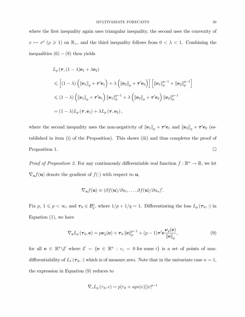
Proof of Proposition 2. For any continuously di¤erentiable real function f : Rn ! R, we let
ruf(u) denote the gradient of f(�) with respect to u,
ruf(u) � (@f(u)=@ui; : : : ; @f(u)=@un)0:
Fix p, 1 6 p < 1, and � 0 2 Bnq , where 1=p + 1=q = 1. Di¤erentiating the loss Lp (� 0; �) in
Equation (1), we have
reLp (� 0; e) = p�p(e) + � 0 kekp�1p + (p� 1)� 0e�p(e)kekp; (9)
for all e 2 RnnE where E = fe 2 R
n : ei = 0 for some ig is a set of points of non-
di¤erentiability of L1 (� 0; �) which is of measure zero. Note that in the univariate case n = 1,
the expression in Equation (9) reduces to
reLp (� 0; e) = p[� 0 + sgn(e)]jejp�1
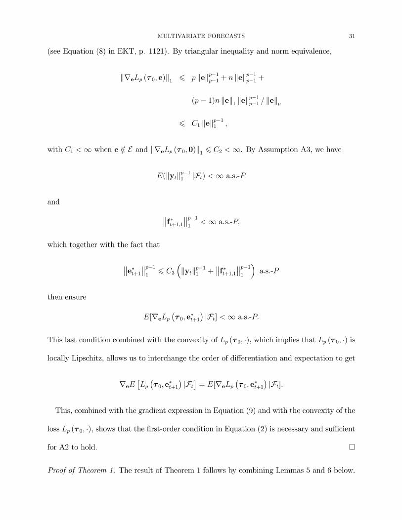
MULTIVARIATE FORECASTS 31
(see Equation (8) in EKT, p. 1121). By triangular inequality and norm equivalence,
kreLp (� 0; e)k1 6 p kekp�1p�1 + n kekp�1p�1 +
(p� 1)n kek1 kekp�1p�1 = kekp
6 C1 kekp�11 ;
with C1 <1 when e =2 E and kreLp (� 0;0)k1 6 C2 <1. By Assumption A3, we have
E(kytkp�11 jFt) <1 a.s.-P
and
f�t+1;1 p�11
<1 a.s.-P;
which together with the fact that
e�t+1 p�11
6 C3
�kytkp�11 +
f�t+1;1 p�11
�a.s.-P
then ensure
E[reLp�� 0; e
�t+1
�jFt] <1 a.s.-P:
This last condition combined with the convexity of Lp (� 0; �), which implies that Lp (� 0; �) is
locally Lipschitz, allows us to interchange the order of di¤erentiation and expectation to get
reE�Lp�� 0; e
�t+1
�jFt�= E[reLp
�� 0; e
�t+1
�jFt]:
This, combined with the gradient expression in Equation (9) and with the convexity of the
loss Lp (� 0; �), shows that the �rst-order condition in Equation (2) is necessary and su¢cient
for A2 to hold. �
Proof of Theorem 1. The result of Theorem 1 follows by combining Lemmas 5 and 6 below.
MULTIVARIATE FORECASTS 32
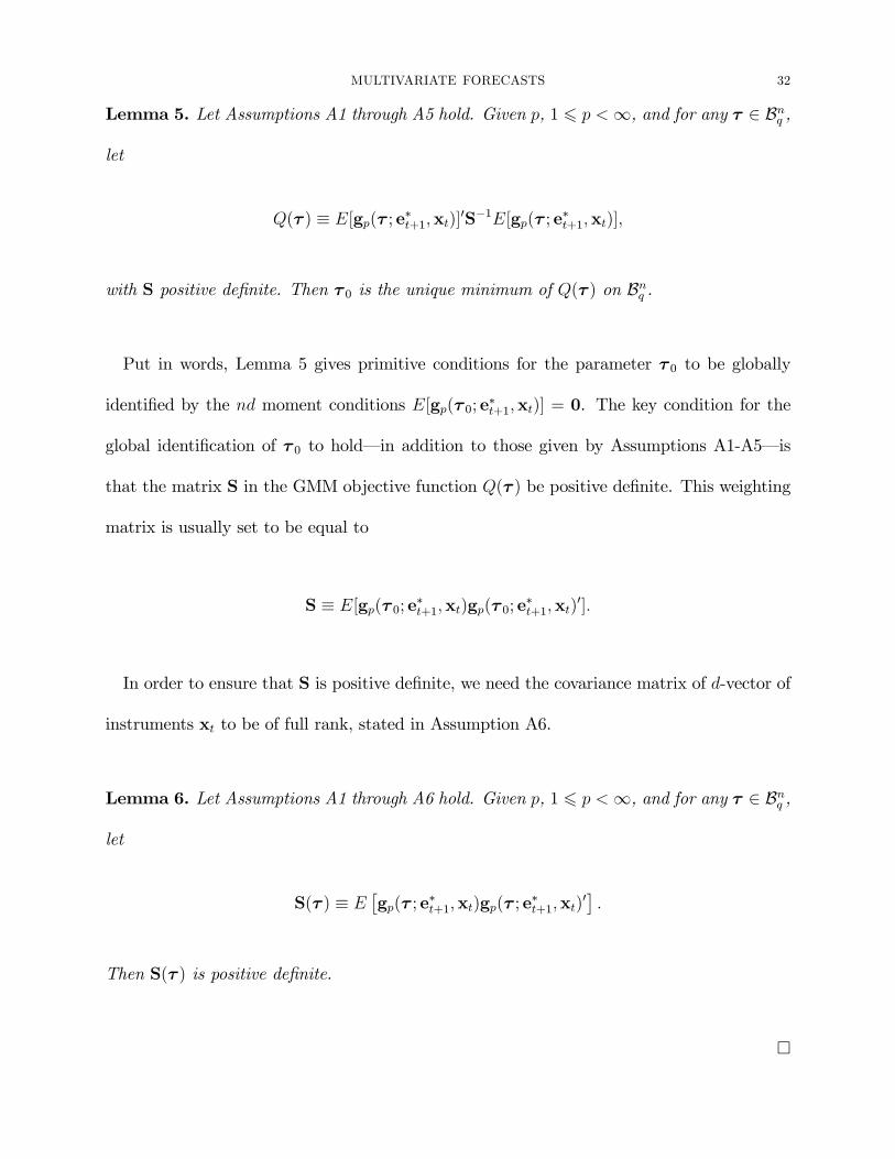
Lemma 5. Let Assumptions A1 through A5 hold. Given p, 1 6 p <1, and for any � 2 Bnq ,
let
Q(� ) � E[gp(� ; e�t+1;xt)]0S�1E[gp(� ; e�t+1;xt)];
with S positive de�nite. Then � 0 is the unique minimum of Q(� ) on Bnq .
Put in words, Lemma 5 gives primitive conditions for the parameter � 0 to be globally
identi�ed by the nd moment conditions E[gp(� 0; e�t+1;xt)] = 0. The key condition for the
global identi�cation of � 0 to hold�in addition to those given by Assumptions A1-A5�is
that the matrix S in the GMM objective function Q(� ) be positive de�nite. This weighting
matrix is usually set to be equal to
S � E[gp(� 0; e�t+1;xt)gp(� 0; e�t+1;xt)0]:
In order to ensure that S is positive de�nite, we need the covariance matrix of d-vector of
instruments xt to be of full rank, stated in Assumption A6.
Lemma 6. Let Assumptions A1 through A6 hold. Given p, 1 6 p <1, and for any � 2 Bnq ,
let
S(� ) � E�gp(� ; e
�t+1;xt)gp(� ; e
�t+1;xt)
0�:
Then S(� ) is positive de�nite.
�
MULTIVARIATE FORECASTS 33
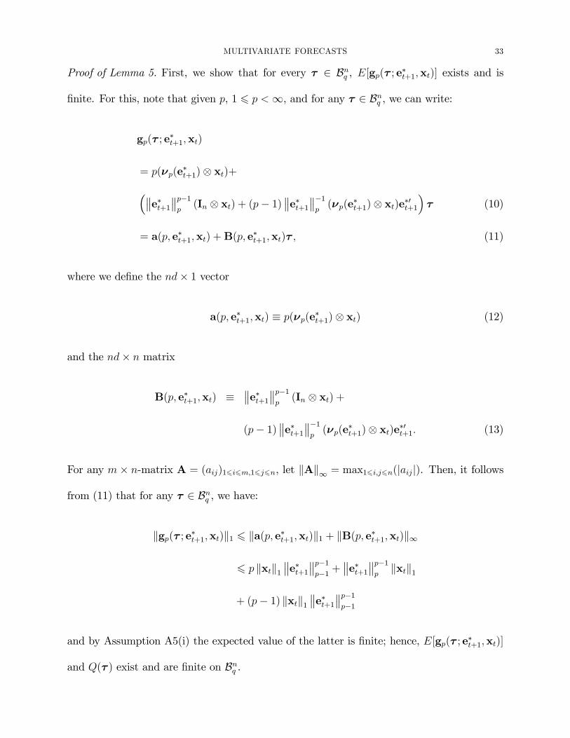
Proof of Lemma 5. First, we show that for every � 2 Bnq , E[gp(� ; e�t+1;xt)] exists and is
�nite. For this, note that given p, 1 6 p <1, and for any � 2 Bnq , we can write:
gp(� ; e�t+1;xt)
= p(�p(e�t+1) xt)+
� e�t+1 p�1p(In xt) + (p� 1)
e�t+1 �1p(�p(e
�t+1) xt)e�0t+1
�� (10)
= a(p; e�t+1;xt) +B(p; e�t+1;xt)� ; (11)
where we de�ne the nd� 1 vector
a(p; e�t+1;xt) � p(�p(e�t+1) xt) (12)
and the nd� n matrix
B(p; e�t+1;xt) � e�t+1
p�1p(In xt) +
(p� 1) e�t+1
�1p(�p(e
�t+1) xt)e�0t+1: (13)
For any m� n-matrix A = (aij)16i6m;16j6n, let kAk1 = max16i;j6n(jaijj). Then, it follows
from (11) that for any � 2 Bnq , we have:
kgp(� ; e�t+1;xt)k1 6 ka(p; e�t+1;xt)k1 + kB(p; e�t+1;xt)k1
6 p kxtk1 e�t+1
p�1p�1
+ e�t+1
p�1pkxtk1
+ (p� 1) kxtk1 e�t+1
p�1p�1
and by Assumption A5(i) the expected value of the latter is �nite; hence, E[gp(� ; e�t+1;xt)]
and Q(� ) exist and are �nite on Bnq .
MULTIVARIATE FORECASTS 34
Given that S (and hence S�1) is positive de�nite, then for any � 2 Bnq we have Q(� ) > 0
with equality if and only if E[gp(� ; e�t+1;xt)] = 0. Now, the optimality condition derived
in Proposition 2 implies that E[gp(� 0; e�t+1;xt)] = 0. Hence, � 0 is a minimum of Q(� ) on
Bnq . We now show that this minimum is moreover unique. For this, we need to show that
E[gp( � ; e�t+1;xt)] = 0 has a unique solution � = � 0. Since
E[gp(� ; e�t+1;xt)] = E[a(p; e
�t+1;xt)] + E[B(p; e
�t+1;xt)]�
a solution is unique if and only if rankE[B(p; e�t+1;xt)] = n; the latter holds under Assump-
tion A5(ii), so � 0 is the unique minimum of Q(� ). �
Proof of Lemma 6. Given p, 1 6 p <1, and for any � 2 Bnq , let
S(� ) � E�gp(� ; e
�t+1;xt)gp(� ; e
�t+1;xt)
0�:
Then
S(� ) = E�reLp(� ; e
�t+1)reLp(� ; e
�t+1)
0 xtx0t�
= E�E�reLp(� ; e
�t+1)reLp(� ; e
�t+1)
0jFt� xtx0t
�:
In order to show that S(� ) is positive de�nite, it su¢ces to show that with probability one:
(i) E�reLp(� ; e
�t+1)reLp(� ; e
�t+1)
0jFt�is positive de�nite, and
(ii) xtx0t is positive de�nite.
The second property holds if E(xtx0t) is of full rank as assumed in A6. We now show
that the �rst property holds as well. Given that the n-variate loss is convex and such that
Lp(� ; e) > 0 with Lp(� ; e) = 0 only if e = 0 (Proposition 1), we have that given Ft,
reLp(� ; e�t+1)reLp(� ; e
�t+1)
0 � 0 a.s.-P

MULTIVARIATE FORECASTS 35
with equality only if reLp(� ; e�t+1) = 0 a.s.-P , i.e., only if e�t+1 = 0 a.s.-P . Since by
Assumption A1 yt is continuously distributed, we have that Pr(e�t+1 = 0jFt) = 0 so
reLp(� ; e�t+1)reLp(� ; e
�t+1)
0 > 0 a.s.-P:
Then, the property (i) holds. Hence, S(� ) is positive de�nite. �
MULTIVARIATE FORECASTS 36
References
[1] Batchelor, R. and D. A. Peel, �Rationality Testing under Asymmetric Loss,� Economic
Letters 61:1 (1998), 49-54.
[2] Bracewell, R. N., The Fourier Transform and Its Applications (New York: MacGraw-
Hill, 1999).
[3] Capistran, C. and A. Timmermann, �Disagreement and Biases in In�ation Expecta-
tions,� Journal of Money, Credit and Banking 41:(2-3) (2009), 365-396.
[4] Christiano, L. J., M. Eichenbaum, and C. L. Evens, �Monetary Policy Shocks: What
Have We Learned and To What End?� (pp. 65-148) in J. B. Taylor and M. Woodford
(Eds.), Handbook of Macroeconomics (Amsterdam: Elsevier, 1999).
[5] Clarida, R., J. Galì, and M. Gertler, �Monetary Policy Rules and Macroeconomic Stabil-
ity: Evidence and Some Theory,�Quarterly Journal of Economics 115:1 (2000), 147-180.
[6] Chaudhuri, P., �On a Geometric Notation of Quantiles for Multivariate Data,� Journal
of the American Statistical Association 91: 434 (1996), 862-872.
[7] Christo¤ersen, P. F. and F. X. Diebold, �Optimal Prediction under Asymmetric Loss,�
Econometric Theory 13:6 (1997), 808-817.
[8] Clark, T. E. and M. W. McCracken, �Tests of Equal Forecast Accuracy and Encom-
passing for Nested Models,� Journal of Econometrics 105:1 (2001), 85-110.
[9] Clark, T. E. and K. D. West, �Using Out-of-Sample Mean Squared Prediction Errors to
Test the Martingale Di¤erence Hypothesis,� Journal of Econometrics 135: (1-2) (2006),
155-186.
[10] �, �Approximately Normal Tests for Equal Predictive Accuracy in Nested Models,�
Journal of Econometrics 138:1 (2007), 291-311.
MULTIVARIATE FORECASTS 37
[11] Corradi, V. and N. R. Swanson, �A consistent Test for Nonlinear Out of Sample Pre-
dictive Accuracy,� Journal of Econometrics 110:2 (2002), 352-381.
[12] �, �Nonparametric Bootstrap Procedures for Predictive Inference Based on Recursive
Estimation Schemes,� International Economic Review 48:1 (2007), 67-109.
[13] �, �Predictive Density and Conditional Con�dence Interval Accuracy Tests,� Journal
of Econometrics 135:(1-2) (2006), 187-228.
[14] Elliott, G., I. Komunjer, and A. Timmermann, �Estimation and Testing of Forecast
Rationality under Flexible Loss,� The Review of Economic Studies 72:4 (2005), 1107-
1125.
[15] �, �Biases in Macroeconomic Forecasts: Irrationality or Asymmetric Loss?� Journal of
the European Economic Association 6:1 (2008), 122-157.
[16] Elliott, G. and A. Timmerman, �Economic Forecasting,� Journal of Economic Literature
46:1 (2008), 3-56.
[17] Figlewski, S. and P. Wachtel, �The Formation of In�ationary Expectations,� Review of
Economics and Statistics, 63:1 (1981), 1-10.
[18] Hansen, L.P., �Large Sample Properties of Generalized Method of Moments Estima-
tors,� Econometrica 50:4 (1982), 1029-1054.
[19] Hardy, G. H., J. E. Littlewood, and George Polya, Inequalities (United Kingdom: Cam-
bridge University Press, 1952).
[20] Hubrich, K. and K. D. West, �Forecast Evaluation of Small Nested Model Sets,� Journal
of Applied Econometrics 25:4 (2010), 574-594.
[21] Koenker, R. and G. Bassett, Jr., �Regression Quantiles,� Econometrica 46:1 (1978),
33-50.
MULTIVARIATE FORECASTS 38
[22] Keane, M. P. and D. E. Runkle, �Testing the Rationality of Price Forecasts: New
Evidence from Panel Data,� American Economic Review 80:4 (1990), 714-735.
[23] Kirchgässner, B. and U. K. Müller, �Are Forecasters Reluctant to Revise their Predica-
tions? Some German Evidence,� Journal of Forecasting 25:6 (2006), 401-413.
[24] Komunjer, I., �Global Identi�cation in Nonlinear Models under Moment Restrictions,�
University of California, San Diego working paper (2011).
[25] Lieli, R. P. and M. B. Stinchcombe, �On the Recoverability of Forecasters� Preferences,�
University of Texas, Austin working paper (2009).
[26] Lucas, R. E. Jr., �Some International Evidence on Output-In�ation Tradeo¤s,� Ameri-
can Economic Review 63:3 (1973), 326-334.
[27] McCracken, M. W., �Robust Out-of-Sample Inference,� Journal of Econometrics 99
(2000), 195-223.
[28] �, �Asymptotics for Out of Sample Tests of Granger Causality,� Journal of Economet-
rics 140 (2007), 719-752.
[29] McCallum, B. T. and Edward Nelson, �An Optimizing IS-LM Speci�cation for Mone-
tary Policy and Business Cycle Analysis,� Journal of Money, Credit, and Banking 31:3
(1999), 296-316.
[30] Mincer, J. and V. Zarnowitz �The Evaluation of Economic Forecasts,� (pp.1-46), in
J. Mincer (Ed.) Economic Forecasts and Expectations (New York: National Bureau of
Economic Research, 1969).
[31] Mishkin, Frank S., �Are Market Forecasts Rational?� American Economic Review 71:3
(1981), 295-306.
MULTIVARIATE FORECASTS 39
[32] Muth, John F., �Rational Expectations and the Theory of Price Movements,� Econo-
metrica 29:3 (1961), 315-335.
[33] Patton, A. J. and A. Timmermann, �Testing Forecast Optimality under Unknown Loss,�
Journal of the American Statistical Association 102 (2007a), 1172-1184.
[34] �, �Properties of Optimal Forecasts under Asymmetric Loss and Nonlinearity,� Journal
of Econometrics 140:2 (2007b), 884-918.
[35] Pesaran, M. H. and Martin Weale, �Survey Expectations� (pp. 715-776), in G. Elliott,
C. W. J. Granger, and A. Timmermann (Eds.) Handbook of Economic Forecasting Vol.
1 (Amsterdam: North-Holland, 2006).
[36] Rockafellar, R. T., Convex Analysis (Princeton, New Jersey: Princeton University Press,
1970).
[37] Theil, H., Economic Forecasts and Policy (Amsterdam: North-Holland, 1958).
[38] Taylor, J. B., �Discretion versus Policy Rules in Practice,� Carnegie-Rochester Confer-
ence series on Public Policy 39:1 (1993): 195-214.
[39] West, K. D. and M. W. McCracken, �Regression-based Tests of Predictive Ability,�
International Economic Review 39 (1998), 817-840.
[40] West, K. D., �Asymptotic Inference About Predictive Ability,� Econometrica 64:5
(1996), 1067-1084.
[41] �, �Forecast Evaluation� (pp. 99-134), in G. Elliott, C. W. J. Granger, and A. Timmer-
mann (Eds.), Handbook of Economic Forecasting (Amsterdam: Elsevier, North-Holland,
2006).
[42] Zarnowtiz, V., �Rational Expectations and Macroeconomic Forecasts,� Journal of Busi-
ness and Economic Statistics 3 (1985), 293-311.
40
[43] Zellner, A., �Biased Predictors, Rationality and the Evaluation of Forecasts,� Economic
Letters 21:1 (1986), 45-48.
Notes
1Another way to test for rationality of forecasts would be to specify an alternative forecast
formation model, such as that of �adaptive� expectations, for example. In that case,
rejections of rationality would be in favor of the speci�c alternative.
2Those results are obtained under a speci�c parametric assumption for the forecasters� loss.
Quantifying the degree of asymmetry of the forecasters� losses in a nonparametric
framework is still an open question. Important nonparametric identi�cation results have
been obtained in Lieli and Stinchcombe (2009) who point out that �[the] cost of this
generality is that [the] identi�cation results are more abstract and do not directly translate
into a strategy for estimation and inference.�
3Strictly speaking, such generalizations will only apply to direct forecasting methods. In
particular, forecasts that are constructed iteratively would require a di¤erent treatment.
4The parameterization in EKT is stated in terms of � = (� + 1)=2 with 0 < � < 1, which is
equivalent.
5The two middle plots in the left panel of Figure 1 illustrate this point. The plots are
obtained when � = (0;�0:5)0 and � = (0:4;�0:3), respectively. In both cases, k�k2 = 0:5;
however, the directions of the two asymmetry vectors are di¤erent, thus resulting in
di¤erent bivariate losses.
6Similarly, we use sgn : R! f�1; 0; 1g to denote the sign function:
sgn(u) = 1I(u)� 1I(�u) = 21I(u)� 1.
41
7In theory, we could estimate the shape of the loss Lp together with its asymmetry
parameter � . However, due to slow convergence speeds, estimation of the shape parameter
is rather unreliable at sample sizes considered in our empirical application.
8The analogous assumption in the decision theoretic literature would be that the decision
maker is an expected utility maximizer. This property, in particular, eliminates objective
functions of the form detE[ et+1e0t+1].
9That S(� 0) is positive de�nite is a condition typically used to show that � 0 is locally
identi�ed.
10The length of the in-sample used for estimation of the forecasting model is denoted by R,
while P stands for the length of the out-of-sample forecasting period. Thus, the length of
the available sample equals T + 1 = R + P .
11If instead of a rolling window scheme, we assumed that the forecasts were constructed
using a recursive scheme (i.e., with an expanding estimation sample ranging from 1 to R
for the �rst forecast, then from 1 to R + 1 for the second forecast, and so on), then fet+1g
would not necessarily inherit the strict stationarity and �-mixing properties of fwtg and
A8 would fail�see West (2006), for example. Similarly, an assumption of �xed forecasting
scheme would make A7 untenable.
12One way to correct for the �many instrument problem� would be to use estimators that are
robust to the presence of many instruments (such as the GEL estimator, for example).
Under many instrument asymptotics, these estimators can be shown to have convenient
Gaussian limit distributions, although the form of the covariance matrix would involve an
extra adjustment term relative to that obtained under the case of conventional
asymptotics, which we maintain here.

42
13These data are taken from the Federal Reserve Bank of St. Louis�s Archival Federal
Reserve Economic Data (ALFRED), available at www.stlsfrb.org. The short-term interest
rate, which is not typically revised, was taken from the Federal Reserve Board.
Figure . Contour plots of the bivariate loss L2(� ; �) with �(� 1; � 2)0 (left),
and of the sum of univariate losses L2(� 1; �)+ L2(� 2; �) (right), with � =
(0; 0)0; (0;�0:5)0; (0:4;�0:3)0; (0:7;�0:5)0 (top to bottom).
MULTIVARIATE FORECASTS 3
-1 -0.5 0 0.5 10
2
4
6
8
10
12
τ
# o
f Fore
caste
rs
τ1
-1 -0.5 0 0.5 10
2
4
6
8
10
12
14
16
18
τ
# o
f Fore
caste
rs
τ2
-1 -0.5 0 0.50
1
2
3
4
5
6
7
8
9
10
τ
# o
f Fore
caste
rs
τ3
Univariate
Multivariate
Figure . Distribution of the asymmetry parameter estimates obtained when
xt = (1;●�Pt)0.
4 IVANA KOMUNJER AND MICHAEL T. OWYANG
0 0.5 10
0.5
1
Separable
No
nse
pa
rab
le
τ1
0 0.5 10
0.5
1
Separable
No
nse
pa
rab
le
τ2
0 0.5 10
0.5
1
Separable
No
nse
pa
rab
le
τ3
0 0.5 10
0.5
1
Separable
No
nse
pa
rab
le
0 0.5 10
0.5
1
SeparableN
onse
pa
rab
le
0 0.5 10
0.5
1
Separable
No
nse
pa
rab
le
0 0.5 10
0.5
1
Separable
No
nse
pa
rab
le
0 0.5 10
0.5
1
Separable
No
nse
pa
rab
le
0 0.5 10
0.5
1
Separable
No
nse
pa
rab
le
0 0.5 10
0.5
1
Separable
No
nse
pa
rab
le
0 0.5 10
0.5
1
Separable
No
nse
pa
rab
le
0 0.5 10
0.5
1
Separable
No
nse
pa
rab
le
0 0.5 10
0.5
1
Separable
No
nse
pa
rab
le
0 0.5 10
0.5
1
Separable
No
nse
pa
rab
le
0 0.5 10
0.5
1
Separable
No
nse
pa
rab
le
Figure . Absolute values of the asymmetry parameter estimates obtained
under separable and nonseparable losses for each instrument set. Circles in-
dicate values for which rationality was accepted at the 95 level using the
nonseparable loss.
R, P τ 1 τ 2 τ 3 SD τ 1 SD τ 2 SD τ 3 R, P τ 1 τ 2 τ 3 SD τ 1 SD τ 2 SD τ 3 J-test
R=250,P=150 -0.003 0.010 0.006 0.072 0.072 0.074 R=250,P=150 0.001 0.011 0.004 0.077 0.075 0.078 0.04
R=250,P=200 -0.003 0.000 0.000 0.060 0.063 0.063 R=250,P=200 -0.003 0.000 0.000 0.063 0.064 0.065 0.03
R=250,P=250 0.002 0.001 -0.001 0.049 0.051 0.046 R=250,P=250 0.002 0.002 -0.001 0.050 0.053 0.049 0.01
R=200,P=250 -0.003 -0.002 -0.001 0.044 0.044 0.044 R=200,P=250 -0.003 -0.003 -0.001 0.046 0.046 0.045 0.00
R=300,P=200 0.000 0.000 0.002 0.063 0.060 0.061 R=300,P=200 0.000 0.000 0.002 0.066 0.063 0.064 0.03
R, P τ 1 τ 2 τ 3 SD τ 1 SD τ 2 SD τ 3 R, P τ 1 τ 2 τ 3 SD τ 1 SD τ 2 SD τ 3 J-test
R=250,P=150 -0.005 -0.007 -0.496 0.070 0.064 0.060 R=250,P=150 -0.002 -0.010 -0.504 0.074 0.068 0.064 0.03
R=250,P=200 0.000 0.000 -0.492 0.054 0.054 0.048 R=250,P=200 0.000 0.000 -0.499 0.058 0.057 0.050 0.03
R=250,P=250 -0.002 -0.002 -0.494 0.046 0.046 0.039 R=250,P=250 -0.002 -0.003 -0.499 0.048 0.047 0.040 0.01
R=200,P=250 -0.001 0.002 -0.492 0.039 0.042 0.035 R=200,P=250 -0.001 0.002 -0.496 0.041 0.044 0.036 0.00
R=300,P=200 0.003 0.001 0.493 0.056 0.055 0.048 R=300,P=200 0.003 0.001 0.500 0.059 0.058 0.049 0.03
R, P τ 1 τ 2 τ 3 SD τ 1 SD τ 2 SD τ 3 R, P τ 1 τ 2 τ 3 SD τ 1 SD τ 2 SD τ 3 J-test
R=250,P=150 0.002 0.392 -0.291 0.066 0.062 0.067 R=250,P=150 0.002 0.400 -0.297 0.069 0.064 0.069 0.02
R=250,P=200 0.002 0.394 -0.296 0.056 0.049 0.052 R=250,P=200 0.002 0.399 -0.300 0.058 0.050 0.054 0.02
R=250,P=250 0.002 0.394 -0.295 0.046 0.042 0.043 R=250,P=250 0.002 0.397 -0.297 0.047 0.043 0.045 0.01
R=200,P=250 -0.002 0.392 -0.296 0.041 0.037 0.039 R=200,P=250 -0.002 0.396 -0.298 0.043 0.038 0.040 0.01
R=300,P=200 -0.005 0.392 -0.299 0.058 0.052 0.054 R=300,P=200 -0.005 0.398 -0.304 0.061 0.054 0.056 0.04
R, P τ 1 τ 2 τ 3 SD τ 1 SD τ 2 SD τ 3 R, P τ 1 τ 2 τ 3 SD τ 1 SD τ 2 SD τ 3 J-test
R=250,P=150 0.001 0.690 -0.495 0.051 0.034 0.042 R=250,P=150 0.000 0.695 -0.500 0.054 0.034 0.042 0.03
R=250,P=200 -0.001 0.696 -0.493 0.040 0.027 0.035 R=250,P=200 -0.001 0.700 -0.496 0.042 0.028 0.036 0.02
R=250,P=250 0.000 0.695 -0.494 0.034 0.024 0.029 R=250,P=250 0.000 0.698 -0.497 0.035 0.025 0.030 0.01
R=200,P=250 -0.001 0.693 -0.496 0.030 0.021 0.026 R=200,P=250 -0.001 0.695 -0.497 0.031 0.022 0.027 0.00
R=300,P=200 -0.002 0.694 -0.499 0.042 0.028 0.035 R=300,P=200 -0.001 0.700 -0.501 0.044 0.029 0.036 0.02
NOTES: This table reports average GMM estimates for τ obtained across 1000 Monte Carlo simulations. Standard deviations are reported in columns
marked SD. J-test represents the percentage of rejections of the null of rationality at the 5% level. τ 0 indicates the true value of τ. R is the size of the
rolling window of data used to construct the forecasts, and P is the size of the evaluation sample.
The parameterization of the VAR(1) that generates the data is:
τ 0 = (0,0.7,-0.5) τ 0 = (0,0.7,-0.5)
τ 0 = (0,0,-0.5) τ 0 = (0,0,-0.5)
τ 0 = (0,0.4,-0.3) τ 0 = (0,0.4,-0.3)
Table 1: GMM Estimator and J-test of rationality (5% Nominal Size)
(a) Instrument = (1) (b) Instrument = (1, y 1,t ); 3 Overidentifying Restrictions
τ 0 = (0,0,0) τ 0 = (0,0,0)
1 3 3, where ~ 0, , 0.01* 1,1,1 , 0.5*I , and 0.01*I .t t t ty c Ay u u N c A
τ 1 τ 2 τ 3 τ 1 τ 2 τ 3 τ 1 τ 2 τ 3
-0.139 -0.943 -0.910 0.003 -0.695 -0.596
(0.102) (0.020) (0.027) (0.044) (0.023) (0.027)
-0.159 -0.952 -0.917 -0.004 -0.699 -0.601
(0.111) (0.022) (0.029) (0.047) (0.024) (0.028)
-0.181 -0.959 -0.930 0.010 -0.702 -0.606
(0.118) (0.021) (0.029) (0.049) (0.025) (0.029)
-0.203 -0.966 -0.939 -0.017 -0.706 -0.610
(0.125) (0.021) (0.030) (0.051) (0.025) (0.029)
-0.159 -0.952 -0.920 -0.038 -0.699 -0.600
(0.112) (0.022) (0.028) (0.047) (0.025) (0.028)
NOTES: This table reports the average estimates for τ computed over 1000 Monte Carlo replications.
Relative MSE is the ratio of the mean squared error MSE = i2 + [Bias(τ i)]
2 from the separable to the nonseparable case.
The parameterization of the VAR(1) that generates the data is:
The instrument sets are: (1) Constant only; (2) Constant and one lag of the first (symmetric loss) variable; (3) Constant
and one lag of the second variable; (4) Constant and one lag of first two variables; and (5) Constant and one lag of all
three variables. Standard deviations are reported in parentheses.
Table 2: Monte Carlo Results
τ 0 = (0,-0.7,-0.6); R = 250; P = 150
Instr SetSeparable Nonseparable Relative MSE
2 17.14 108.61 134.23
1 15.09 109.79 132.98
18.49 106.49 128.50
5 16.88 106.24 131.97
4 20.06 105.25 122.48
3
1
1 0.5 0.2 0.14 1 0.9 0.171 1
, where ~ 0, , 1 , 0.2 0.5 0.14 , and 0.9 1 0.46 .100 100
1 0.14 0.14 0.5 0.17 0.46 1
t t t ty c Ay u u N c A

Instr Set Constant GDP/GNP CPI Unemp Short Rate
1 1 n/a n/a n/a n/a
2 1 n/a 1 n/a n/a
3 1 n/a n/a n/a 1
4 1 1 n/a n/a n/a
5 1 n/a n/a 1 n/a
NOTES: The table reflects the lags of variables used as instruments.
n/a indicates the variable is not included in the instrument set.
GDP/GNP, CPI, and unemployment are taken as rates. The short rate
is the 3 month T-bill rate.
Table 3: Instrument Sets

10% 5% 1% 10% 5% 1% 10% 5% 1%
2 0.30 0.18 0.00 0.30 0.18 0.04 1.00 0.99 0.97
3 0.47 0.28 0.07 0.56 0.33 0.07 1.00 1.00 1.00
4 0.14 0.02 0.00 0.14 0.04 0.00 1.00 0.99 0.94
5 0.86 0.77 0.32 0.91 0.70 0.21 1.00 1.00 0.99
NOTES: This table reports the percentages of forecasters for whom the null of rationality and nonseparable loss
(left), rationality and separable loss (middle), and rationality and separable symmetric loss (right) could be rejected
at the specified levels. The results are obtained by fixing p=2 . The instrument sets are as defined in Table 3.
Table 4: J-tests of Rationality
Instr Set
Rejections of Rationality
Nonseparable Loss Separable Loss Separable Symmetric Loss
τ y τ π τ r ||τ||2 τ y τ π τ r ||τ||21 -0.053 0.118 -0.419 0.513 -0.075 0.137 -0.439 0.515
2 -0.094 0.194 -0.452 0.577 -0.062 0.206 -0.429 0.582
3 -0.098 0.150 -0.460 0.575 -0.093 0.141 -0.483 0.587
4 -0.069 0.154 -0.430 0.543 -0.070 0.165 -0.440 0.539
5 0.021 0.186 -0.550 0.652 0.056 0.244 -0.535 0.665
τ y τ π τ r ||τ||2 τ y τ π τ r ||τ||21 -0.074 0.213 -0.496 0.680 -0.105 0.215 -0.509 0.673
2 -0.096 0.392 -0.527 0.817 -0.097 0.456 -0.520 0.798
3 -0.141 0.260 -0.544 0.784 -0.141 0.243 -0.561 0.764
4 -0.083 0.295 -0.503 0.735 -0.054 0.323 -0.508 0.700
5 0.034 0.499 -0.645 0.947 0.089 0.639 -0.633 0.949
NOTES: This table reports summary statistics of GMM estimates of τ obtained across forecasters. GNP (y )
and inflation (π ) are taken as growth rates. The short rate (r ) is the 3-month T-bill rate. The results are
obtained by fixing p=2. The instrument sets are as defined in Table 3. For the first instrument set, means and
medians are taken over the entire sample of valid forecasters. For all other instrument sets, they are computed
only for those forecasters for whom the null of rationality could not be rejected at the 5% level.
Table 5: Estimated Asymmetry Coefficients under Separable and Nonseparable Loss
Nonseparable
Separable
Inst Set
Inst SetMeans
Means Medians
Medians
ONLINE APPENDI MULTIVARIATE FORECAST EVALUATION
AND RATIONALITY TESTING
IVANA KOMUNJER AND MICHAEL T. OWYANG
This online appendix consists of three parts. Section 1 of the appendix contains ad-
ditional information on the forecast data used in the empirical application (Section 6 of
the paper). Section 2 of the appendix gives detailed proofs of Theorems 2 and 3 stated
in the main text (Section 4 of the paper). Finally, the last part of the appendix contains
additional panels of Table 1 discussed in the Monte Carlo experiment (Section 5.1 of the
paper).
1. Information on t e CEI Forecast ata
In the empirical section of the paper, we use individual forecaster�s forecasts from the
Blue Chip Economic Indicators (BCEI). The data is proprietary. The survey reports
monthly updates of forecasts from individual forecasters starting in 1976:08. Prior to
1984, �rms reported current-year forecasts for the �rst �ve or six months of the year.
In later months, they reported next-year forecasts. Starting in 1984, both current- and
next-year forecasts were reported each month.
We use forecasts for three variables: output, in�ation, and a short-term interest rate.
The sample of output forecasts is split between GNP (1976:08 through 1991:12) and
GDP (1992:01 through 2004:12). The BCEI began collecting CPI in�ation forecasts in
1979:01 through the end of our sample in 2004:12. The short-term interest rate forecasts
are split between the 3-month commercial paper (1976:08 through 1980:06), the 6-month
commercial paper (1980:07 through 1981:12), and the 3-month T-bill (1982:01 through
2004:12) rates. For output and in�ation, the target variable is the rate of change between
the average of the levels for that year. This method is described by the BCEI in their
monthly newsletter.
1
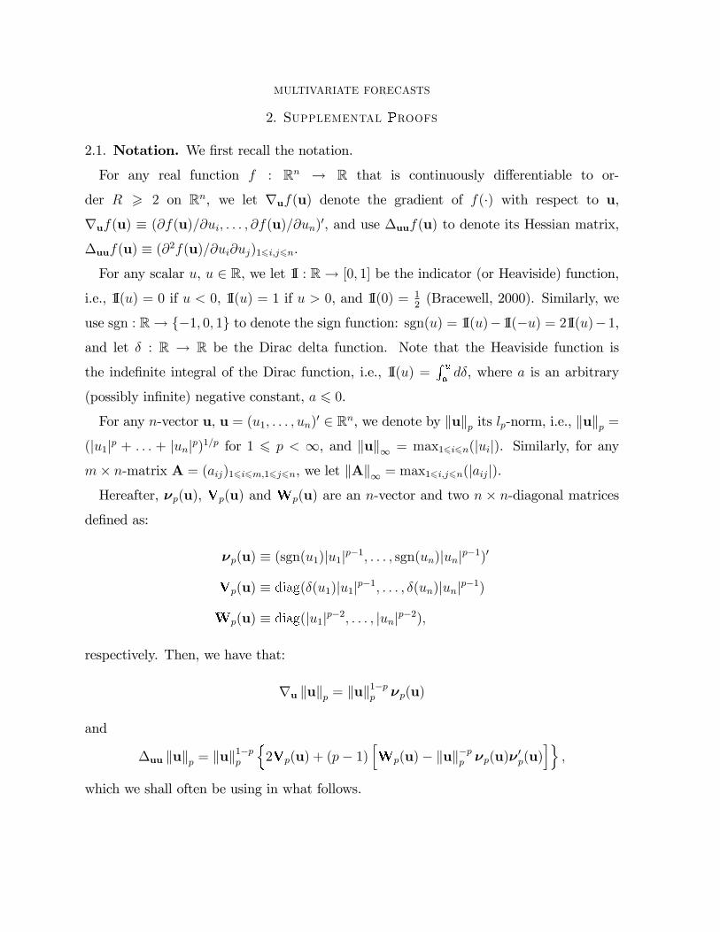
MULTIVARIATE FORECASTS 2
2. Supplemental roofs
2.1. Notation. We �rst recall the notation.
For any real function f : Rn ! R that is continuously di¤erentiable to or-
der R > 2 on Rn, we let ruf(u) denote the gradient of f(�) with respect to u,ruf(u) � (@f(u)=@ui; : : : ; @f(u)=@un)0, and use �uuf(u) to denote its Hessian matrix,
�uuf(u) � (@2f(u)=@ui@uj)16i;j6n.For any scalar u, u 2 R, we let 1I : R! [0; 1] be the indicator (or Heaviside) function,
i.e., 1I(u) = 0 if u < 0, 1I(u) = 1 if u > 0, and 1I(0) = 12(Bracewell, 2000). Similarly, we
use sgn : R! f�1; 0; 1g to denote the sign function: sgn(u) = 1I(u)�1I(�u) = 21I(u)�1,and let � : R ! R be the Dirac delta function. Note that the Heaviside function is
the inde�nite integral of the Dirac function, i.e., 1I(u) =✉
❛d�, where a is an arbitrary
(possibly in�nite) negative constant, a 6 0.
For any n-vector u, u = (u1; : : : ; un)0 2 Rn, we denote by kukp its lp-norm, i.e., kukp =
(ju1jp + : : : + junjp)1=p for 1 6 p < 1, and kuk1 = max16i6n(juij). Similarly, for anym� n-matrix A = (aij)16i6m;16j6n, we let kAk1 = max16i;j6n(jaijj).Hereafter, �p(u), ❱p(u) and ❲p(u) are an n-vector and two n � n-diagonal matrices
de�ned as:
�p(u) � (sgn(u1)ju1jp�1; : : : ; sgn(un)junjp�1)0
❱p(u) � ❞✁✂✄(�(u1)ju1jp�1; : : : ; �(un)junjp�1)
❲p(u) � ❞✁✂✄(ju1jp�2; : : : ; junjp�2);
respectively. Then, we have that:
ru kukp = kuk1�pp �p(u)
and
�uu kukp = kuk1�pp 2❱p(u) + (p� 1)
h❲p(u)� kuk�pp �p(u)�
0p(u)
io;
which we shall often be using in what follows.
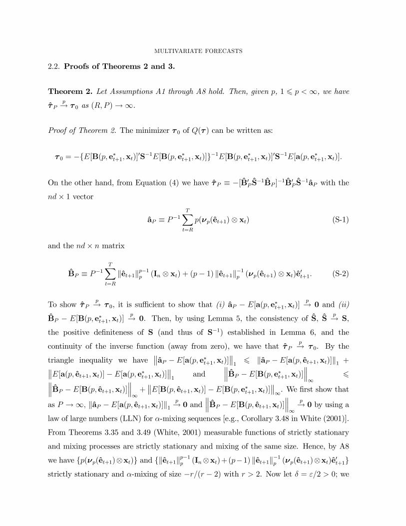
MULTIVARIATE FORECASTS 3
2.2. Proofs of Theorems 2 and 3.
Theorem 2. Let Assumptions A1 through A8 hold. Then, given p, 1 6 p <1, we have�P
p! � 0 as (R;P )!1.
Proof of Theorem 2. The minimizer � 0 of Q(� ) can be written as:
� 0 = �fE[B(p; e�t+1;xt)]0S�1E[B(p; e�t+1;xt)]g�1E[B(p; e�t+1;xt)]0S�1E[a(p; e�t+1;xt)]:
On the other hand, from Equation (4) we have �P � �[B0P S�1BP ]�1B0P S�1aP with thend� 1 vector
aP � P�1TX
t=R
p(�p(et+1) xt) (S-1)
and the nd� n matrix
BP � P�1TX
t=R
ket+1kp�1p (In xt) + (p� 1) ket+1k�1p (�p(et+1) xt)e0t+1: (S-2)
To show �Pp! � 0, it is su¢cient to show that (i) aP � E[a(p; e�t+1;xt)]
p! 0 and (ii)
BP � E[B(p; e�t+1;xt)]p! 0. Then, by using Lemma 5, the consistency of S, S
p! S,
the positive de�niteness of S (and thus of S�1) established in Lemma 6, and the
continuity of the inverse function (away from zero), we have that �Pp! � 0. By the
triangle inequality we have aP � E[a(p; e�t+1;xt)]
16 kaP � E[a(p; et+1;xt)]k1 + E[a(p; et+1;xt)]� E[a(p; e�t+1;xt)]
1
and BP � E[B(p; e�t+1;xt)]
1
6 BP � E[B(p; et+1;xt)]
1+ E[B(p; et+1;xt)]� E[B(p; e�t+1;xt)]
1. We �rst show that
as P !1; kaP � E[a(p; et+1;xt)]k1p! 0 and
BP � E[B(p; et+1;xt)] 1
p! 0 by using a
law of large numbers (LLN) for �-mixing sequences [e.g., Corollary 3.48 in White (2001)].
From Theorems 3.35 and 3.49 (White, 2001) measurable functions of strictly stationary
and mixing processes are strictly stationary and mixing of the same size. Hence, by A8
we have fp(�p(et+1)xt)g and fket+1kp�1p (Inxt)+(p�1) ket+1k�1p (�p(et+1)xt)e0t+1gstrictly stationary and �-mixing of size �r=(r � 2) with r > 2. Now let � = "=2 > 0; we
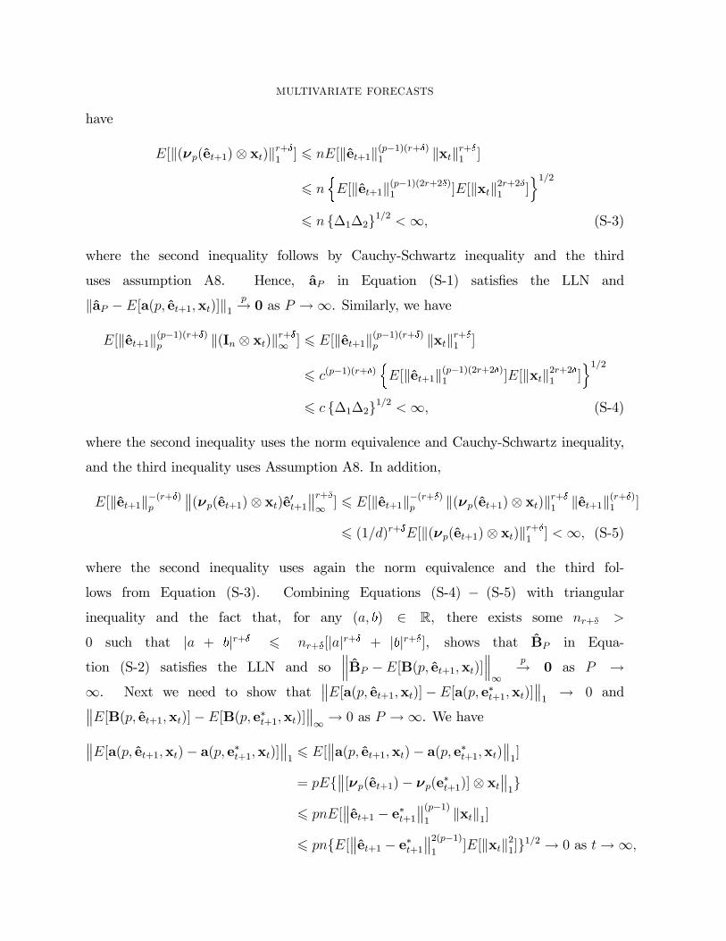
MULTIVARIATE FORECASTS 4
have
E[k(�p(et+1) xt)kr+✍1 ] 6 nE[ket+1k(p�1)(r+✍)1 kxtkr+✍1 ]
6 n E[ket+1k(p�1)(2r+2✍)1 ]E[kxtk2r+2✍1 ]o1=2
6 n f�1�2g1=2 <1; (S-3)
where the second inequality follows by Cauchy-Schwartz inequality and the third
uses assumption A8. Hence, aP in Equation (S-1) satis�es the LLN and
kaP � E[a(p; et+1;xt)]k1p! 0 as P !1. Similarly, we have
E[ket+1k(p�1)(r+✍)p k(In xt)kr+✍1 ] 6 E[ket+1k(p�1)(r+✍)p kxtkr+✍1 ]
6 c(p�1)(r+✍) E[ket+1k(p�1)(2r+2✍)1 ]E[kxtk2r+2✍1 ]o1=2
6 c f�1�2g1=2 <1; (S-4)
where the second inequality uses the norm equivalence and Cauchy-Schwartz inequality,
and the third inequality uses Assumption A8. In addition,
E[ket+1k�(r+✍)p
(�p(et+1) xt)e0t+1 r+✍1] 6 E[ket+1k�(r+✍)p k(�p(et+1) xt)kr+✍1 ket+1k(r+✍)1 ]
6 (1=d)r+✍E[k(�p(et+1) xt)kr+✍1 ] <1; (S-5)
where the second inequality uses again the norm equivalence and the third fol-
lows from Equation (S-3). Combining Equations (S-4) � (S-5) with triangular
inequality and the fact that, for any (a; ❜) 2 R, there exists some nr+✍ >
0 such that ja + ❜jr+✍ 6 nr+✍[jajr+✍ + j❜jr+✍], shows that BP in Equa-
tion (S-2) satis�es the LLN and so BP � E[B(p; et+1;xt)]
1
p! 0 as P !1. Next we need to show that
E[a(p; et+1;xt)]� E[a(p; e�t+1;xt)] 1! 0 and
E[B(p; et+1;xt)]� E[B(p; e�t+1;xt)] 1! 0 as P !1. We have
E[a(p; et+1;xt)� a(p; e�t+1;xt)] 16 E[
a(p; et+1;xt)� a(p; e�t+1;xt) 1]
= pEf [�p(et+1)� �p(e�t+1)] xt
1g
6 pnE[ et+1 � e�t+1
(p�1)1
kxtk1]
6 pnfE[ et+1 � e�t+1
2(p�1)1
]E[kxtk21]g1=2 ! 0 as t!1;
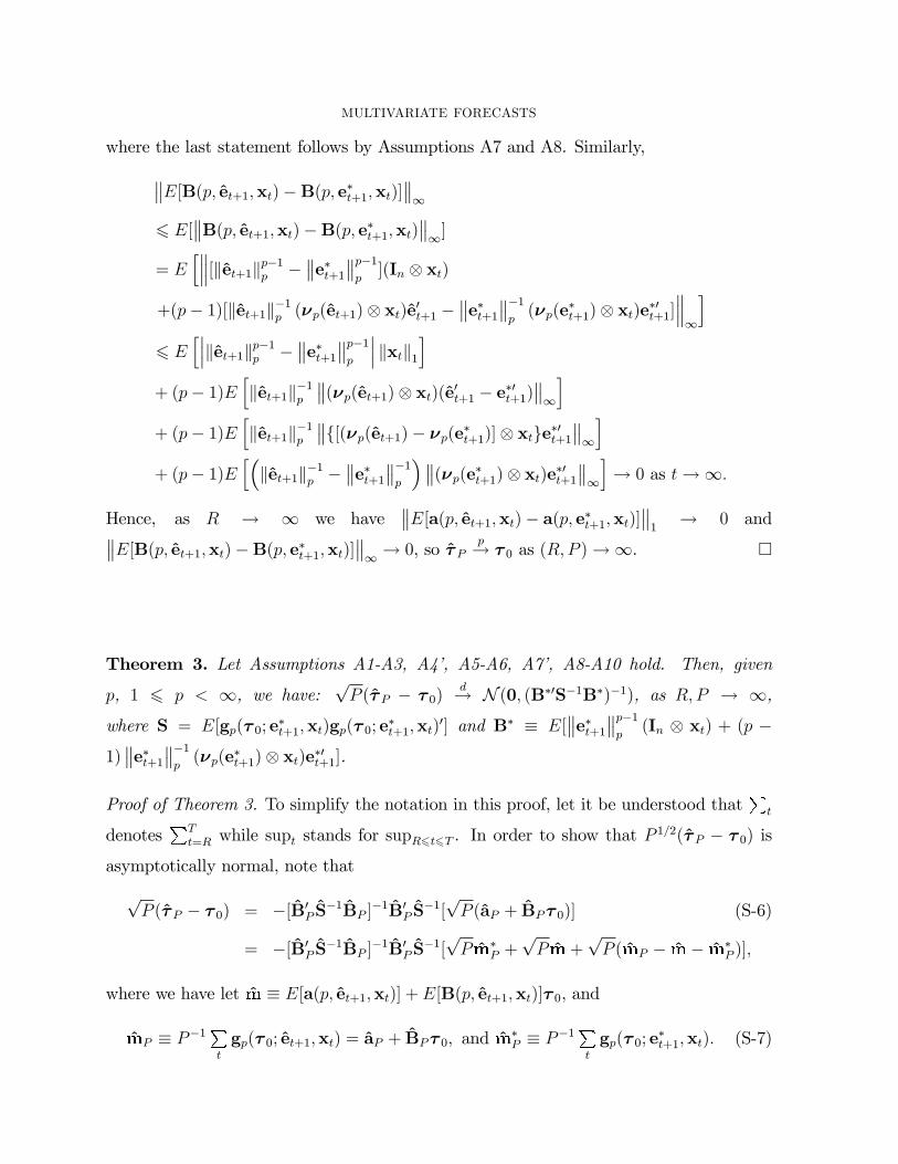
MULTIVARIATE FORECASTS 5
where the last statement follows by Assumptions A7 and A8. Similarly,
E[B(p; et+1;xt)�B(p; e�t+1;xt)] 1
6 E[ B(p; et+1;xt)�B(p; e�t+1;xt)
1]
= Eh [ket+1kp�1p �
e�t+1 p�1p](In xt)
+(p� 1)[ket+1k�1p (�p(et+1) xt)e0t+1 � e�t+1
�1p(�p(e
�t+1) xt)e�0t+1]
1
i
6 Eh���ket+1kp�1p �
e�t+1 p�1p
��� kxtk1i
+ (p� 1)Ehket+1k�1p
(�p(et+1) xt)(e0t+1 � e�0t+1) 1
i
+ (p� 1)Ehket+1k�1p
f[(�p(et+1)� �p(e�t+1)] xtge�0t+1 1
i
+ (p� 1)Eh�ket+1k�1p �
e�t+1 �1p
� (�p(e�t+1) xt)e�0t+1 1
i! 0 as t!1:
Hence, as R ! 1 we have E[a(p; et+1;xt)� a(p; e�t+1;xt)]
1
! 0 and E[B(p; et+1;xt)�B(p; e�t+1;xt)]
1! 0, so �P
p! � 0 as (R;P )!1. �
Theorem 3. Let Assumptions A1-A3, A4�, A5-A6, A7�, A8-A10 hold. Then, given
p, 1 6 p < 1, we have:pP (�P � � 0)
d! N (0; (B�0S�1B�)�1), as R;P ! 1,where S = E[gp(� 0; e
�t+1;xt)gp(� 0; e
�t+1;xt)
0] and B� � E[ e�t+1
p�1p(In xt) + (p �
1) e�t+1
�1p(�p(e
�t+1) xt)e�0t+1].
Proof of Theorem 3. To simplify the notation in this proof, let it be understood that t
denotes Tt=R while supt stands for supR6t6T . In order to show that P
1=2(�P � � 0) isasymptotically normal, note that
pP (�P � � 0) = �[B0P S�1BP ]�1B0P S�1[
pP (aP + BP� 0)] (S-6)
= �[B0P S�1BP ]�1B0P S�1[pP♠�
P +pP♠+
pP (♠P � ♠� ♠�
P )];
where we have let ♠ � E[a(p; et+1;xt)] + E[B(p; et+1;xt)]� 0, and
♠P � P�1t
gp(� 0; et+1;xt) = aP + BP� 0; and ♠�P � P�1
t
gp(� 0; e�t+1;xt): (S-7)
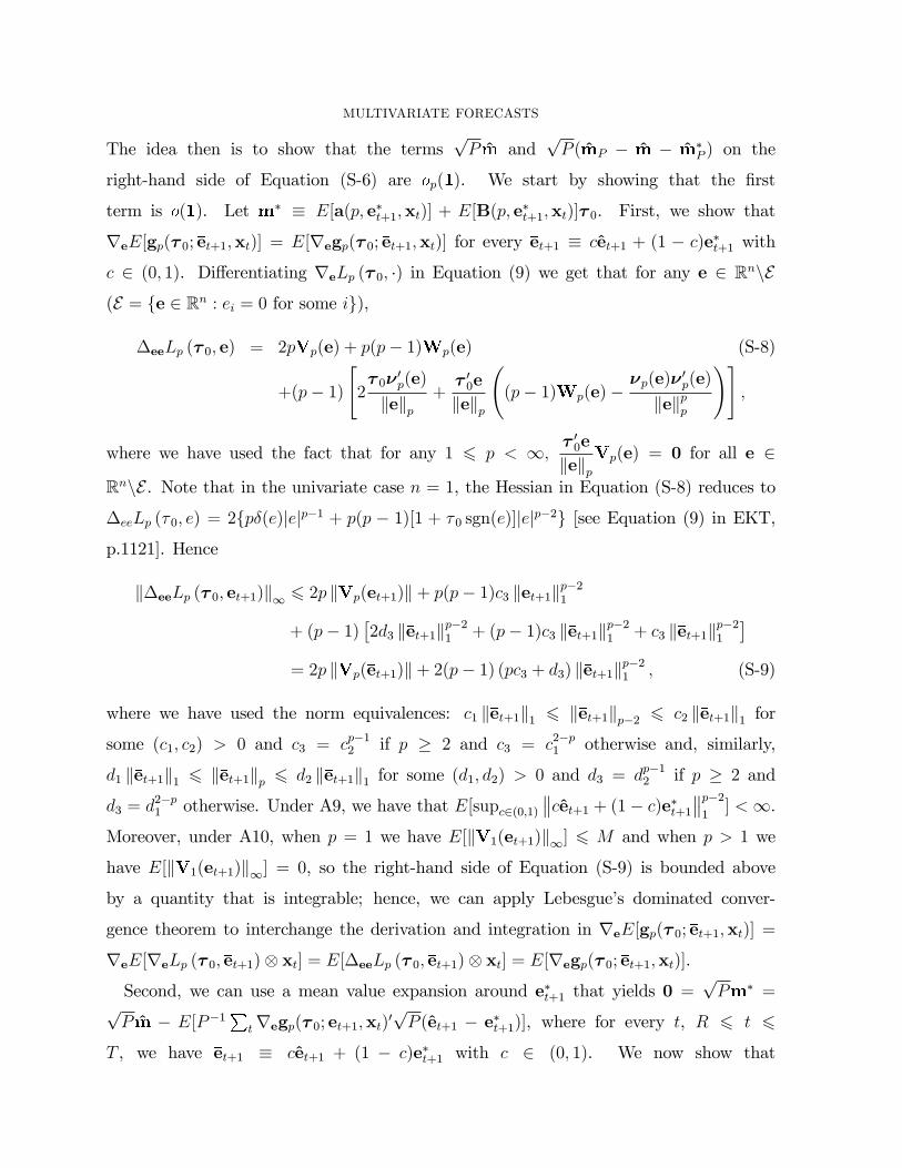
MULTIVARIATE FORECASTS 6
The idea then is to show that the termspP☎ and
pP (☎P � ☎ � ☎
�P ) on the
right-hand side of Equation (S-6) are ♦p(✶). We start by showing that the �rst
term is ♦(✶). Let ☎� � E[a(p; e�t+1;xt)] + E[B(p; e�t+1;xt)]� 0. First, we show that
reE[gp(� 0;✖et+1;xt)] = E[regp(� 0;✖et+1;xt)] for every ✖et+1 � cet+1 + (1 � c)e�t+1 withc 2 (0; 1). Di¤erentiating reLp (� 0; �) in Equation (9) we get that for any e 2 RnnE(E = fe 2 Rn : ei = 0 for some ig),
�eeLp (� 0; e) = 2p✆p(e) + p(p� 1)✝p(e) (S-8)
+(p� 1)"2� 0�
0p(e)
kekp+�00e
kekp
(p� 1)✝p(e)�
�p(e)�0p(e)
kekpp
!#;
where we have used the fact that for any 1 6 p < 1; �00e
kekp✆p(e) = 0 for all e 2
RnnE . Note that in the univariate case n = 1, the Hessian in Equation (S-8) reduces to�eeLp (� 0; e) = 2fp�(e)jejp�1 + p(p � 1)[1 + � 0 sgn(e)]jejp�2g [see Equation (9) in EKT,p.1121]. Hence
k�eeLp (� 0;✖et+1)k1 6 2p k✆p(✖et+1)k+ p(p� 1)c3 k✖et+1kp�21
+ (p� 1)�2d3 k✖et+1kp�21 + (p� 1)c3 k✖et+1kp�21 + c3 k✖et+1kp�21
�
= 2p k✆p(✖et+1)k+ 2(p� 1) (pc3 + d3) k✖et+1kp�21 ; (S-9)
where we have used the norm equivalences: c1 k✖et+1k1 6 k✖et+1kp�2 6 c2 k✖et+1k1 forsome (c1; c2) > 0 and c3 = cp�12 if p � 2 and c3 = c2�p1 otherwise and, similarly,
d1 k✖et+1k1 6 k✖et+1kp 6 d2 k✖et+1k1 for some (d1; d2) > 0 and d3 = dp�12 if p � 2 and
d3 = d2�p1 otherwise. Under A9, we have that E[supc2(0;1)
cet+1 + (1� c)e�t+1 p�21] <1.
Moreover, under A10, when p = 1 we have E[k✆1(✖et+1)k1] 6 M and when p > 1 we
have E[k✆1(✖et+1)k1] = 0, so the right-hand side of Equation (S-9) is bounded above
by a quantity that is integrable; hence, we can apply Lebesgue�s dominated conver-
gence theorem to interchange the derivation and integration in reE[gp(� 0;✖et+1;xt)] =
reE[reLp (� 0;✖et+1) xt] = E[�eeLp (� 0;✖et+1) xt] = E[regp(� 0;✖et+1;xt)].
Second, we can use a mean value expansion around e�t+1 that yields 0 =pP☎� =
pP☎ � E[P�1 tregp(� 0;✖et+1;xt)
0pP (et+1 � e�t+1)], where for every t, R 6 t 6
T , we have ✖et+1 � cet+1 + (1 � c)e�t+1 with c 2 (0; 1). We now show that
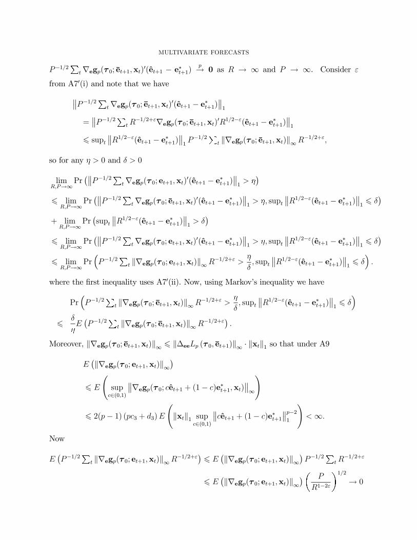
MULTIVARIATE FORECASTS 7
P�1=2 tregp(� 0;✞et+1;xt)0(et+1 � e�t+1)
p! 0 as R ! 1 and P ! 1. Consider "
from A70(i) and note that we have
P�1=2 tregp(� 0;✞et+1;xt)0(et+1 � e�t+1)
1
= P�1=2 tR
�1=2+"regp(� 0;✞et+1;xt)0R1=2�"(et+1 � e�t+1)
1
6 supt R1=2�"(et+1 � e�t+1)
1P�1=2 t kregp(� 0;✞et+1;xt)k1R�1=2+";
so for any ✑ > 0 and � > 0
limR;P!1
Pr� P�1=2 tregp(� 0;✞et+1;xt)
0(et+1 � e�t+1) 1> ✑�
6 limR;P!1
Pr� P�1=2 tregp(� 0;✞et+1;xt)
0(et+1 � e�t+1) 1> ✑; supt
R1=2�"(et+1 � e�t+1) 16 ��
+ limR;P!1
Pr�supt
R1=2�"(et+1 � e�t+1) 1> ��
6 limR;P!1
Pr� P�1=2 tregp(� 0;✞et+1;xt)
0(et+1 � e�t+1) 1> ✑; supt
R1=2�"(et+1 � e�t+1) 16 ��
6 limR;P!1
Pr�P�1=2 t kregp(� 0;✞et+1;xt)k1R�1=2+" >
✑
�; supt
R1=2�"(et+1 � e�t+1) 16 ��:
where the �rst inequality uses A70(ii). Now, using Markov�s inequality we have
Pr�P�1=2 t kregp(� 0;✞et+1;xt)k1R�1=2+" >
✑
�; supt
R1=2�"(et+1 � e�t+1) 16 ��
6�
✑E�P�1=2 t kregp(� 0;✞et+1;xt)k1R�1=2+"
�:
Moreover, kregp(� 0;✞et+1;xt)k1 6 k�eeLp (� 0;✞et+1)k1 � kxtk1 so that under A9
E�kregp(� 0;✞et+1;xt)k1
�
6 E
supc2(0;1)
regp(� 0; cet+1 + (1� c)e�t+1;xt) 1
!
6 2(p� 1) (pc3 + d3)E kxtk1 sup
c2(0;1)
cet+1 + (1� c)e�t+1 p�21
!<1:
Now
E�P�1=2 t kregp(� 0;✞et+1;xt)k1R�1=2+"
�6 E
�kregp(� 0;✞et+1;xt)k1
�P�1=2 tR
�1=2+"
6 E�kregp(� 0;✞et+1;xt)k1
� P
R1�2"
1=2
! 0
MULTIVARIATE FORECASTS 8
as R ! 1 and P ! 1, where the last limit results uses A70(i): HencepP✟ ! 0 as
R!1 and P !1. The termpP (✟P � ✟� ✟
�P ) on the right-hand side of Equation
(S-6) is ✠p(✡) provided that g satis�es a certain Lipshitz condition (given below) and that
A70 holds. Using a reasoning similar to that above, we have any ☛ > 0 and � > 0
limR;P!1
Pr�P 1=2 k✟P � ✟� ✟
�Pk1 > ☛
�
6 limR;P!1
Pr�P 1=2 k✟P � ✟� ✟
�Pk1 > ☛; suptR
1=2�" et+1 � e�t+1
16 ��:
Now, let rP (�) � supfrt+1(et+1) : et+1 � e�t+1
16 �; R 6 t 6 Tg, where we let
rt+1(et+1) (S-10)
� gp(� 0; et+1;xt)� gp(� 0; e�t+1;xt)� [�eeLp
�� 0; e
�t+1
� xt](et+1 � e�t+1)
1 et+1 � e�t+1
1
;
where �eeLp�� 0; e
�t+1
�is as de�ned in Equation (S-8). Then, by the de�nition of
rt+1(et+1),
P 1=2 k✟P � ✟� ✟�Pk1
6 P 1=2 P�1 t[�eeLp
�� 0; e
�t+1
� xt](et+1 � e�t+1)� Ef[�eeLp
�� 0; e
�t+1
� xt](et+1 � e�t+1)g
1
+ P�1 t rt+1(et+1) et+1 � e�t+1
1+ E
�rt+1(et+1)
et+1 � e�t+1 1
�o
6 P 1=2 P�1 t
[�eeLp�� 0; e
�t+1
� xt]� Ef[�eeLp
�� 0; e
�t+1
� xt]g
1supt
et+1 � e�t+1 1
+ [rP (�R) + E(rP (�R))] supt et+1 � e�t+1
1
o
and so by the Markov inequality
Pr�P 1=2 k✟P � ✟� ✟
�Pk1 > ☛; suptR
1=2�" et+1 � e�t+1
16 ��
6P
R1�2"
1=2�
☛
hE�P�1
t
[�eeLp�� 0; e
�t+1
� xt]� Ef[�eeLp
�� 0; e
�t+1
� xt]g
1
�
+ E�rP (�R) + E(rP (�R))
�i:
Using standard arguments for stochastic equicontinuity such as those given in Andrews
(1994), we can show that rt+1(et+1)! 0 as Pr( et+1 � e�t+1
1> ")! 0 for any " > 0, so
that rP (�)! 0 with probability 1, which by the dominated convergence theorem ensures
MULTIVARIATE FORECASTS 9
E(rP (�))! 0. Next, we show that the sample mean of f�eeLp�� 0; e
�t+1
�xtg converges
in probability to its expected value. By assumption A40 we know that f�eeLp�� 0; e
�t+1
�
xtg is strictly stationary and �-mixing with � of size �r=(r�2) with r > 2 [see Theorems3.35 and 3.49 in White (2001)]. Moreover, for � = minf"=2; �=2g > 0 in assumptions A40
and A8, we have
E[ �eeLp
�� 0; e
�t+1
� xt
r+☞1]
6 fE[ �eeLp
�� 0; e
�t+1
� 2r+2☞1
]E[kxtk2r+2☞1 ]g1=2
6
�maxfE[
�eeLp�� 0; e
�t+1
� 2r+�1
]; 1g�1=2 �
maxfE[kxtk2r+"1 ]; 1g�1=2
<1;
since from Equation (S-9) we know
�eeLp�� 0; e
�t+1
� 2r+�1
6 nrf[2p]2r+� ✌p(e
�t+1) 2r+�1
+ [2(p� 1) (pc3 + d3)]2r+� e�t+1
(p�2)(2r+�)1
g;
where again nr is such that for any (a; ✎) > 0 we have (a + ✎)2r+� 6 nr(a2r+� + ✎
2r+�);
and A10 and A40 imply that E[ ✌1(e
�t+1) 2r+�1
] 6 M , E[ ✌p(e
�t+1) 2r+�1
] = 0 and
E[ e�t+1
(p�2)(2r+�)1
] < 1: Using the weak LLN for �-mixing sequences [e.g., Corollary
3.48 in White (2001)] then gives
P�1TX
t=R
�eeLp�� 0; e
�t+1
� xt p! E[�eeLp
�� 0; e
�t+1
� xt]
as P !1. Then, combining all of the above with A70(ii) gives
limR;P!1
PrpP k✏P � ✏� ✏
�Pk1 > ✒; sup
R6t6TR1=2�"
et+1 � e�t+1 16 � = 0
and the termpP (✏P � ✏ � ✏
�P ) on the right-hand side of Equation (S-6) is ✓p(✔)
as R ! 1 and P ! 1. Finally, we use the central limit theorem (CLT) for strictly
stationary and �-mixing sequences [e.g., Theorem 5.20 in White (2001)] to show thatpP✏�
Pd! N (0;S). Using Theorems 3.35 and 3.49 in White (2001), which together show
that time-invariant measurable functions of strictly stationary and mixing sequences are
strictly stationary and mixing of the same size, we know by A40 that fgp(� 0; e�t+1;xt)gis strictly stationary and �-mixing with mixing coe¢cient of size �r=(r � 2), r > 2. In
MULTIVARIATE FORECASTS 10
the proof of Theorem 2 we have moreover shown that E[ gp(� 0; e�t+1;xt)
r+"1] <1. The
CLT [e.g., Theorem 5.20 in White (2001)] then ensures
pP✕�
Pd! N (0;S): (S-11)
The remainder of the asymptotic normality proof is similar to the standard case: the
positive de�niteness of S�1, Sp! S and BP
p! B� � E[B(p; e�t+1;xt)] as R ! 1 and
P !1 (B was de�ned in Equation (12)) together with A5(ii) ensure that (B�0S�1B�)�1
exists, so by usingpP (�P�� 0) = �[B0P S�1BP ]�1B0P S�1[
pP✕�
P+✗p(✘)], the limit result
in (S-11) and the Slutsky theorem we havepP (�P � � 0) d! N (0; (B�0S�1B�)�1), which
completes the proof of asymptotic normality. �
References
[1] Andrews, Donald W. K., Asymptotics for Semiparametric Econometric Models via
Stochastic Equicontinutiy, Econometrica 71:1 (1994), 43-72.
[2] Bracewell, Robert N., The Fourier Transform and Its Applications (New York:
MacGraw-Hill, 1999).
[3] White, Halbert, Asymptotic Theory for Econometricians (San Diego: Academic Press,
2001).