Embed Size (px)
Citation preview
NUMERICAL ANALYSIS OF BACKWARD-FACING
STEP FLOW PRECEEDING A POROUS MEDIUM
USING FLUENT
By
CHANDRAMOULEE KRISHNAMOORTHY
Bachelor of Engineering
University of Mumbai (Bombay)
Mumbai, India
2004
Submitted to the Faculty of the Graduate College of the
Oklahoma State University in partial fulfillment of the requirements for
the Degree of MASTER OF SCIENCE
December, 2007
ii
NUMERICAL ANALYSIS OF BACKWARD-FACING
STEP FLOW PRECEEDING A POROUS MEDIUM
USING FLUENT
Thesis Approved:
Frank W. Chambers
David G. Lilley
Afshin J. Ghajar
A. Gordon Emslie
Dean of the Graduate College
iii
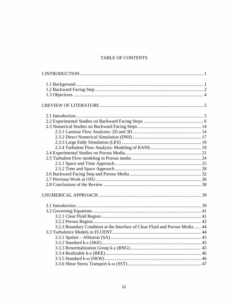
TABLE OF CONTENTS
1.INTRODUCTION ........................................................................................................... 1
1.1 Background............................................................................................................... 1 1.2 Backward Facing Step .............................................................................................. 2 1.3 Objectives ................................................................................................................. 4
2.REVIEW OF LITERATURE .......................................................................................... 5
2.1 Introduction............................................................................................................... 5 2.2 Experimental Studies on Backward Facing Steps .................................................... 6 2.3 Numerical Studies on Backward Facing Steps ....................................................... 14
2.3.1 Laminar Flow Analyses: 2D and 3D ........................................................... 14 2.3.2 Direct Numerical Simulation (DNS) ........................................................... 17 2.3.3 Large Eddy Simulation (LES) .....................................................................19 2.3.4 Turbulent Flow Analysis: Modeling of RANS............................................ 19
2.4 Experimental Studies on Porous Media.................................................................. 21 2.5 Turbulent Flow modeling in Porous media ............................................................ 24
2.5.1 Space and Time Approach........................................................................... 25 2.5.2 Time and Space Approach........................................................................... 28
2.6 Backward Facing Step and Porous Media .............................................................. 32 2.7 Previous Work at OSU............................................................................................ 36 2.8 Conclusions of the Review ..................................................................................... 38
3.NUMERICAL APPROACH ......................................................................................... 39
3.1 Introduction............................................................................................................. 39 3.2 Governing Equations .............................................................................................. 41
3.2.1 Clear Fluid Region....................................................................................... 41 3.2.2 Porous Region.............................................................................................. 42 3.2.3 Boundary Condition at the Interface of Clear Fluid and Porous Media ...... 44
3.3 Turbulence Models in FLUENT............................................................................. 44 3.3.1 Spalart – Allmaras (SA)............................................................................... 45 3.3.2 Standard k-ε (SKE) ...................................................................................... 45 3.3.3 Renormalization Group k-ε (RNG).............................................................. 45 3.3.4 Realizable k-ε (RKE)................................................................................... 46 3.3.5 Standard k-ω (SKW).................................................................................... 46 3.3.6 Shear Stress Transport k-ω (SST)................................................................ 47
iv
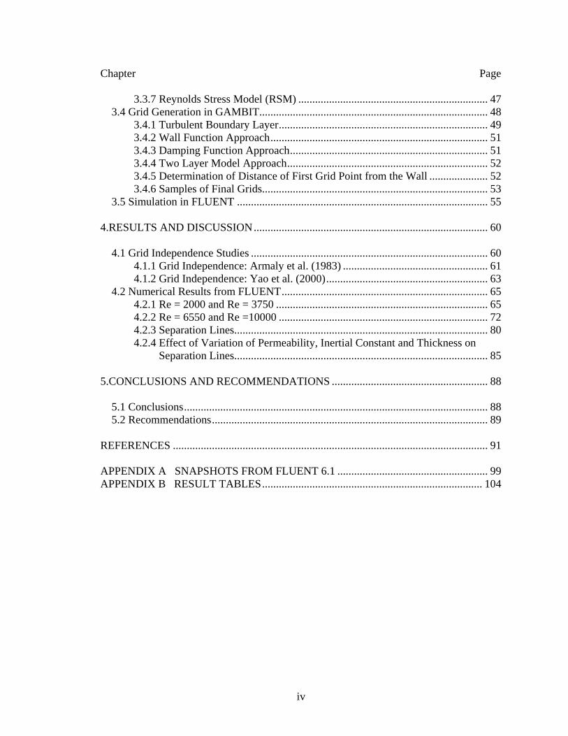
Chapter Page 3.3.7 Reynolds Stress Model (RSM) .................................................................... 47
3.4 Grid Generation in GAMBIT.................................................................................. 48 3.4.1 Turbulent Boundary Layer........................................................................... 49 3.4.2 Wall Function Approach.............................................................................. 51 3.4.3 Damping Function Approach.......................................................................51 3.4.4 Two Layer Model Approach........................................................................52 3.4.5 Determination of Distance of First Grid Point from the Wall ..................... 52 3.4.6 Samples of Final Grids................................................................................. 53
3.5 Simulation in FLUENT .......................................................................................... 55 4.RESULTS AND DISCUSSION.................................................................................... 60
4.1 Grid Independence Studies ..................................................................................... 60 4.1.1 Grid Independence: Armaly et al. (1983) .................................................... 61 4.1.2 Grid Independence: Yao et al. (2000).......................................................... 63
4.2 Numerical Results from FLUENT.......................................................................... 65 4.2.1 Re = 2000 and Re = 3750 ............................................................................ 65 4.2.2 Re = 6550 and Re =10000 ........................................................................... 72 4.2.3 Separation Lines........................................................................................... 80 4.2.4 Effect of Variation of Permeability, Inertial Constant and Thickness on
Separation Lines........................................................................................... 85 5.CONCLUSIONS AND RECOMMENDATIONS ........................................................ 88
5.1 Conclusions............................................................................................................. 88 5.2 Recommendations................................................................................................... 89
REFERENCES ................................................................................................................. 91 APPENDIX A SNAPSHOTS FROM FLUENT 6.1 ...................................................... 99 APPENDIX B RESULT TABLES............................................................................... 104
v
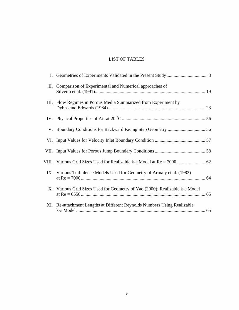
LIST OF TABLES
I. Geometries of Experiments Validated in the Present Study................................... 3
II. Comparison of Experimental and Numerical approaches of Silveira et al. (1991).............................................................................................. 19
III. Flow Regimes in Porous Media Summarized from Experiment by
Dybbs and Edwards (1984)................................................................................... 23
IV. Physical Properties of Air at 20 oC ....................................................................... 56
V. Boundary Conditions for Backward Facing Step Geometry ................................ 56
VI. Input Values for Velocity Inlet Boundary Condition ........................................... 57
VII. Input Values for Porous Jump Boundary Conditions ........................................... 58 VIII. Various Grid Sizes Used for Realizable k-ε Model at Re = 7000 ........................ 62
IX. Various Turbulence Models Used for Geometry of Armaly et al. (1983)
at Re = 7000.......................................................................................................... 64
X. Various Grid Sizes Used for Geometry of Yao (2000); Realizable k-ε Model at Re = 6550.......................................................................................................... 65
XI. Re-attachment Lengths at Different Reynolds Numbers Using Realizable
k-ε Model .............................................................................................................. 65
vi
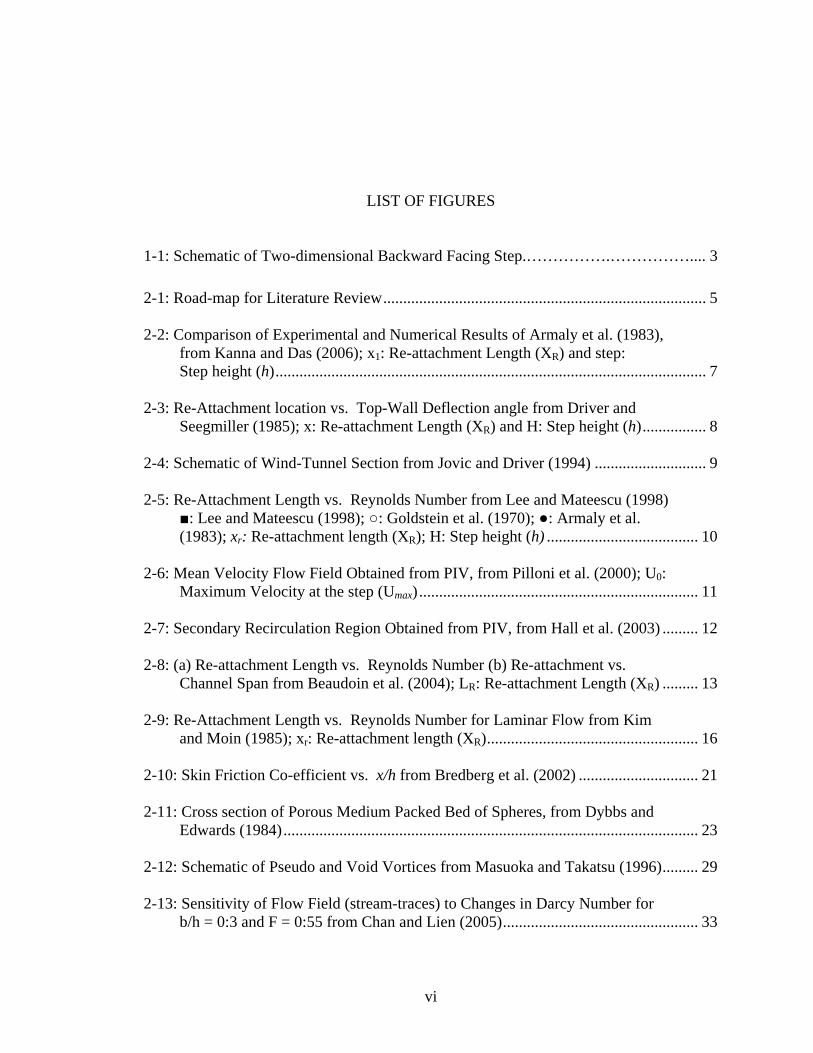
LIST OF FIGURES
1-1: Schematic of Two-dimensional Backward Facing Step.…………….…………….... 3
2-1: Road-map for Literature Review................................................................................. 5 2-2: Comparison of Experimental and Numerical Results of Armaly et al. (1983), from Kanna and Das (2006); x1: Re-attachment Length (XR) and step: Step height (h)............................................................................................................ 7 2-3: Re-Attachment location vs. Top-Wall Deflection angle from Driver and Seegmiller (1985); x: Re-attachment Length (XR) and H: Step height (h)................ 8 2-4: Schematic of Wind-Tunnel Section from Jovic and Driver (1994) ............................ 9 2-5: Re-Attachment Length vs. Reynolds Number from Lee and Mateescu (1998) ■: Lee and Mateescu (1998); ○: Goldstein et al. (1970); ●: Armaly et al. (1983); xr: Re-attachment length (XR); H: Step height (h)...................................... 10 2-6: Mean Velocity Flow Field Obtained from PIV, from Pilloni et al. (2000); U0:
Maximum Velocity at the step (Umax)...................................................................... 11 2-7: Secondary Recirculation Region Obtained from PIV, from Hall et al. (2003) ......... 12 2-8: (a) Re-attachment Length vs. Reynolds Number (b) Re-attachment vs. Channel Span from Beaudoin et al. (2004); LR: Re-attachment Length (XR) ......... 13 2-9: Re-Attachment Length vs. Reynolds Number for Laminar Flow from Kim and Moin (1985); xr: Re-attachment length (XR)..................................................... 16 2-10: Skin Friction Co-efficient vs. x/h from Bredberg et al. (2002) .............................. 21
2-11: Cross section of Porous Medium Packed Bed of Spheres, from Dybbs and Edwards (1984)........................................................................................................ 23 2-12: Schematic of Pseudo and Void Vortices from Masuoka and Takatsu (1996)......... 29 2-13: Sensitivity of Flow Field (stream-traces) to Changes in Darcy Number for b/h = 0:3 and F = 0:55 from Chan and Lien (2005)................................................. 33
vii
Figure Page
2-14: Sensitivity of Flow Field (stream-traces) to Changes in the Forchheimer’s Constant for b/h = 0:3 and Da = 0:01 from Chan and Lien (2005) ......................... 33 2-15: Sensitivity of Flow Field to changes in the Thickness of Porous Insert for Da = 0:01 and F = 0:1 from Chan and Lien (2005) ................................................. 34 2-16: Comparison of Streamlines Between the Linear and Nonlinear Models for Backward-facing-step Flow with Porous Insert, α = 10–6 m2, φ = 0.65 from Assato et al. (2005) ......................................................................................... 35 2-17: Comparison of Streamlines Between the Linear and Nonlinear Models for Backward-facing-step Flow with Porous Insert, α = 10–6 m2, φ = 0.85 from Assato et al. (2005) ......................................................................................... 35 2-18: Comparison of Streamlines Between the Linear and Nonlinear Models for Backward-facing-step Flow with Porous Insert, α = 10–7 m2, φ = 0.85 from Assato et al. (2005) ......................................................................................... 36 3-1: The CFD Simulation Pipeline for Fluent Preprocessing-2006 (Fluent Inc.)............. 41 3-2: Boundary Conditions of the Edges in GAMBIT.......................................................41 3-3: Turbulent Boundary Layer Profile in the Near-wall Region..................................... 50 3-4: Reτ as a Function of Reynolds number from Pope (2000) …………………………53
3-5: Sample Structured Grid of Armaly et al. (1983)....................................................... 54 3-6: Sample Structured Grid of Yao (2000) – No Filter case........................................... 54 3-7: Sample Clustered Grid of Yao (2000) – Filter at 4.25 Step Heights......................... 54 4-1: Separation Lines at Re = 2000: FLUENT ................................................................. 67 4-2: Comparison of Experiment and FLUENT: No Filter Case, Re = 2000 .................... 68 4-3: Comparison of Experiment and FLUENT: Filter at 4.25 h, Re = 2000 .................... 68 4-4: Comparison of Experiment and FLUENT: Filter at 6.75 h, Re = 2000 .................... 69 4-5: Separation Lines at Re = 3750: FLUENT ................................................................. 70 4-6: Comparison of Experiment and FLUENT: No Filter Case, Re = 3750 .................... 70
viii
Figure Page 4-7: Comparison of Experiment and FLUENT: Filter at 4.25 h, Re = 3750 .................... 71 4-8: Comparison of Experiment and FLUENT: Filter at 6.75 h, Re = 3750 .................... 71 4-9: Separation Lines at Re = 6550: FLUENT ................................................................. 72 4-10: Comparison of Experiment and FLUENT: No Filter Case, Re = 6550 .................. 74
4-11: Comparison of Experiment and FLUENT: Filter at 4.25 h, Re = 6550 .................. 74 4-12: Comparison of Experiment and FLUENT: Filter at 6.75 h, Re = 6550 .................. 75 4-13: FLUENT Velocity Profiles at 3.75 h; With and Without Filter at 4.25 h, Re = 6550................................................................................................................. 75 4-14: FLUENT Velocity Profiles at 5h; With and Without Filter at 6.75 h, Re = 6550................................................................................................................. 76 4-15: Separation Lines at Re = 10000: FLUENT ............................................................. 77 4-16: Comparison of Experiment and FLUENT: No Filter case, Re = 10000 ................. 77 4-17: Comparison of Experiment and FLUENT: Filter at 4.25 h, Re = 10000 ................ 78 4-18: Comparison of Experiment and FLUENT: Filter at 6.75 h, Re = 10000 ................ 79 4-19: FLUENT Velocity Profiles at 3.75 h: With and Without Filter at 4.25 h, Re = 10000............................................................................................................... 79 4-20: FLUENT Velocity Profiles at 6.25 h: With and Without Filter at 6.75 h, Re = 10000............................................................................................................... 80
4-21: Separation Lines for No Filter Case: Yao (2000).................................................... 81 4-22: Separation Lines for No Filter Case: FLUENT....................................................... 81 4-23: Separation Lines for Filter at 4.25 h: Yao (2000) ................................................... 83 4-24: Separation Lines for Filter at 4.25 h: FLUENT...................................................... 83 4-25: Separation Lines for Filter at 6.75 h: Yao (2000) ................................................... 84 4-26: Separation Lines for Filter at 6.75 h: FLUENT...................................................... 84
ix
Figure Page 4-27: Effect of Variation of Permeability (α) on Separation Lines by FLUENT; Inertial Constant (C2) = 4.533*103 1/m, Thickness (b) = 15 mm for Filter Placed at 4.25 h: Re=10000………………………………………………………..86 4-28: Effect of Variation of Inertial Constant (C2) on Separation Lines by FLUENT;
Permeability (α) = 1.17*10-9 m2, Thickness (b) = 15 mm for Filter Placed at 4.25 h: Re=10000 ..................................................................................... 86
4-29: Effect of Variation of Thickness (b) on Separation Lines by FLUENT;
Permeability (α) = 1.17*10-9 m2, Inertial Constant (C2) = 4.533*103 1/m
for Filter Placed at 4.25h: Re=10000.……………………….………….……….....87

x
NOMENCLATURE
b Thickness of porous inserts
Cf Skin friction coefficient
Cε Coefficient determined from experiment
C2 Pressure jump coefficient
dP Characteristic length of pore
Dh Hydraulic diameter
Da Darcy number
F Forchheimer’s constant
F Body force vector
g Gravity vector
h Step height
I Identity matrix
k Kinetic energy
p Pressure
Re Reynolds number
Reh Reynolds number based on step height
ReP Pore Reynolds number
τRe Reynolds number based on uτ
s Channel height
xi
t Time
iu Velocity in primary direction
iu Mean velocity in primary direction
iu′ Velocity fluctuation in primary direction
u+ Dimensionless wall velocity
uτ Friction velocity
Ubulk Bulk velocity of the flow
Uinlet Boundary condition input at the inlet of channel
Umax Maximum velocity at step
UP Fluid velocity through pore
U Mean velocity
v Velocity
X Length in X-direction
x1 Re-attachment length
xi Primary direction
xj Other direction
XR Re-attachment length
Y Length in Y-direction
yP Actual distance from the wall
+y Wall units
z Width in Z-direction
α Permeability of the filter
δij Kronecker delta
xii
∆p Pressure drop
ε Turbulence dissipation
κ Log-law coefficient
ϕ Porosity of the filter
ρ Fluid density
τ Stress tensor
µ Dynamic viscosity
ν Kinematic viscosity
Tν Turbulent viscosity
ω Specific dissipation rate
∇ Del operator
ABBREVIATIONS
AR Aspect Ratio
CFD Computational Fluid Dynamics
DES Detached Eddy Simulation
DNS Direct Numerical Simulation
ER Expansion Ratio
LDA Laser Doppler Anemometer
LDV Laser Doppler Velocimeter
LES Large Eddy Simulation
LIF Laser Induced Fluorescence
xiii
N-S Navier Stokes
PDE Partial Differential Equation
PIV Particle Image Velocimetry
PVC Poly Vinyl Chloride
RANS Reynolds Averaged Navier Stokes
RNG Renormalization Group
RSM Reynolds Stress Model
SA Spalart Allmaras
SKE Standard k-ε
SKW Standard k-ω
SST Shear Stress Transport k-ω
1
CHAPTER 1
INTRODUCTION
1.1 Background One of the important engineering applications, where the fluid flows through unexpected
bends and encounters sudden expansions is the ‘air filter housings’ of automobiles. The
rationale behind this complex flow path in present day automobiles is that the design
criteria are determined by space utilization rather than fluid mechanics. This
arrangement results in the flow being non-uniform and the mean velocity of the flow is
not normal to the surface of the filter. Moreover, the velocity fluctuations observed in
the separation region combined with non-uniform flow are found to be detrimental to the
performance of the filter. Previous research has shown that the velocity fluctuations and
non-uniform flow through the filter are the important factors on which the filtration
efficiency depends. The real flow field through air filter housing, when considered with
all its geometrical parameters is extremely intricate and expensive to simulate
numerically. Also, it is not feasible to measure all the minute details of the real flow
field. Thus, the need to build a simplified model of this complex flow that will result in a
better understanding of the interaction between the separation region and the porous
medium is highlighted in this research. For some engineering applications, the above
phenomena (separation and re-attachment) facilitates in enhancing the momentum, heat
and/or mass transfer rates while for the others, it may lead to an unsteady flow resulting
2
in noise, vibration and reduced efficiency. Other significant applications of flow
modeling through porous media can be found in designs of fluidized bed combustors,
catalytic reactors, crude-oil drilling, flows in the core of nuclear reactors and
environmental flows over forests and vegetation. Hence, turbulent flow modeling in
porous media is an essential exercise in understanding various complex engineering and
environmental flows.
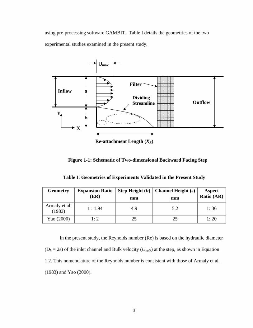
1.2 Backward Facing Step
The backward-facing step flow (see Figure 1-1) is a fundamental flow that
provides a simple geometry to serve as a prototype for studying complex phenomena like
flow separation and re-attachment. It is similar to many industrial flows, including
housings for automotive air filters and headers for compact cross flow heat exchangers.
A comprehensive understanding of these phenomena is of prime importance for the
design of engineering devices like diffusers, turbines, combustors, airfoils, etc.
Figure 1.1 shows a two-dimensional schematic of a backward facing step with a
porous insert. The channel height is denoted by‘s’ and step-height is denoted by ‘h’. The
expansion ratio (ER) is then defined as shown in Equation 1.1.
hs
sER
+= (1.1)
In the present study the step-flow experiments of Armaly et al. (1983) and Yao
(2000) were modeled using commercial software FLUENT and the mesh was created
3
using pre-processing software GAMBIT. Table I details the geometries of the two
experimental studies examined in the present study.
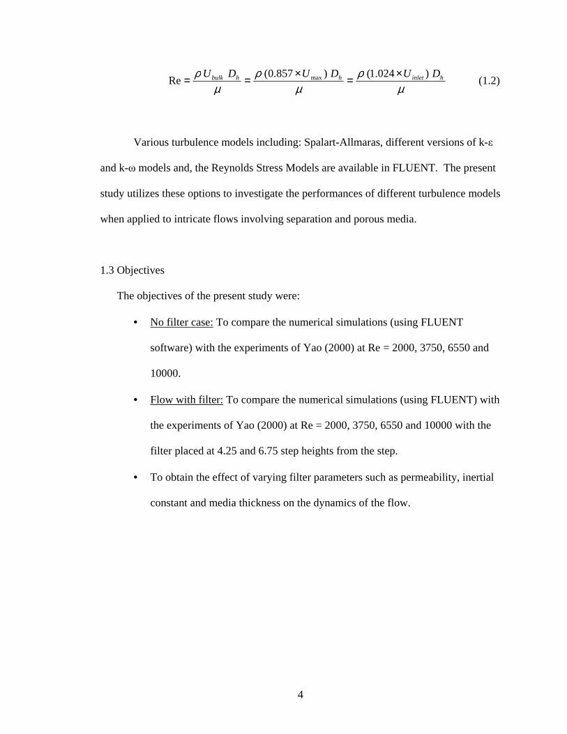
Table I: Geometries of Experiments Validated in the Present Study
Geometry Expansion Ratio
(ER) Step Height (h)
mm
Channel Height (s)
mm
Aspect Ratio (AR)
Armaly et al. (1983)
1 : 1.94 4.9 5.2 1: 36
Yao (2000) 1: 2 25 25 1: 20
In the present study, the Reynolds number (Re) is based on the hydraulic diameter
(Dh = 2s) of the inlet channel and Bulk velocity (Ubulk) at the step, as shown in Equation
1.2. This nomenclature of the Reynolds number is consistent with those of Armaly et al.
(1983) and Yao (2000).
Inflow
Outflow Dividing Streamline
Re-attachment Length (XR)
Y
X
Filter
h
s
Umax
Figure 1-1: Schematic of Two-dimensional Backward Facing Step
4
µ
ρµ
ρµ
ρ hinlethhbulk DUDUDU )024.1()857.0(Re max ×=×== (1.2)
Various turbulence models including: Spalart-Allmaras, different versions of k-ε
and k-ω models and, the Reynolds Stress Models are available in FLUENT. The present
study utilizes these options to investigate the performances of different turbulence models
when applied to intricate flows involving separation and porous media.
1.3 Objectives
The objectives of the present study were:
• No filter case: To compare the numerical simulations (using FLUENT
software) with the experiments of Yao (2000) at Re = 2000, 3750, 6550 and
10000.
• Flow with filter: To compare the numerical simulations (using FLUENT) with
the experiments of Yao (2000) at Re = 2000, 3750, 6550 and 10000 with the
filter placed at 4.25 and 6.75 step heights from the step.
• To obtain the effect of varying filter parameters such as permeability, inertial
constant and media thickness on the dynamics of the flow.
5
CHAPTER 2
REVIEW OF LITERATURE
2.1 Introduction
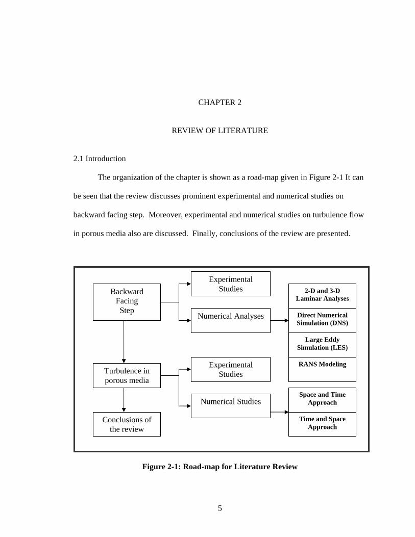
The organization of the chapter is shown as a road-map given in Figure 2-1 It can
be seen that the review discusses prominent experimental and numerical studies on
backward facing step. Moreover, experimental and numerical studies on turbulence flow
in porous media also are discussed. Finally, conclusions of the review are presented.
Figure 2-1: Road-map for Literature Review
Backward Facing Step
Experimental Studies
Numerical Analyses
2-D and 3-D Laminar Analyses Direct Numerical Simulation (DNS)
Large Eddy
Simulation (LES)
RANS Modeling
Conclusions of the review
Turbulence in porous media
Experimental Studies
Numerical Studies Space and Time
Approach
Time and Space Approach
6
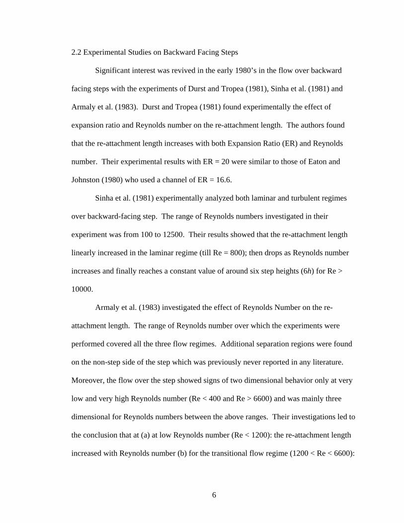
2.2 Experimental Studies on Backward Facing Steps
Significant interest was revived in the early 1980’s in the flow over backward
facing steps with the experiments of Durst and Tropea (1981), Sinha et al. (1981) and
Armaly et al. (1983). Durst and Tropea (1981) found experimentally the effect of
expansion ratio and Reynolds number on the re-attachment length. The authors found
that the re-attachment length increases with both Expansion Ratio (ER) and Reynolds
number. Their experimental results with ER = 20 were similar to those of Eaton and
Johnston (1980) who used a channel of ER = 16.6.
Sinha et al. (1981) experimentally analyzed both laminar and turbulent regimes
over backward-facing step. The range of Reynolds numbers investigated in their
experiment was from 100 to 12500. Their results showed that the re-attachment length
linearly increased in the laminar regime (till Re = 800); then drops as Reynolds number
increases and finally reaches a constant value of around six step heights (6h) for Re >
10000.
Armaly et al. (1983) investigated the effect of Reynolds Number on the re-
attachment length. The range of Reynolds number over which the experiments were
performed covered all the three flow regimes. Additional separation regions were found
on the non-step side of the step which was previously never reported in any literature.
Moreover, the flow over the step showed signs of two dimensional behavior only at very
low and very high Reynolds number (Re < 400 and Re > 6600) and was mainly three
dimensional for Reynolds numbers between the above ranges. Their investigations led to
the conclusion that at (a) at low Reynolds number (Re < 1200): the re-attachment length
increased with Reynolds number (b) for the transitional flow regime (1200 < Re < 6600):
7
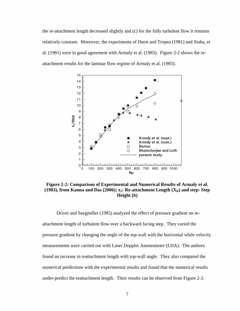
the re-attachment length decreased slightly and (c) for the fully turbulent flow it remains
relatively constant. Moreover, the experiments of Durst and Tropea (1981) and Sinha, et
al. (1981) were in good agreement with Armaly et al. (1983). Figure 2-2 shows the re-
attachment results for the laminar flow regime of Armaly et al. (1983).
Figure 2-2: Comparison of Experimental and Numerical Results of Armaly et al. (1983), from Kanna and Das (2006); x1: Re-attachment Length (XR) and step: Step
Height (h)
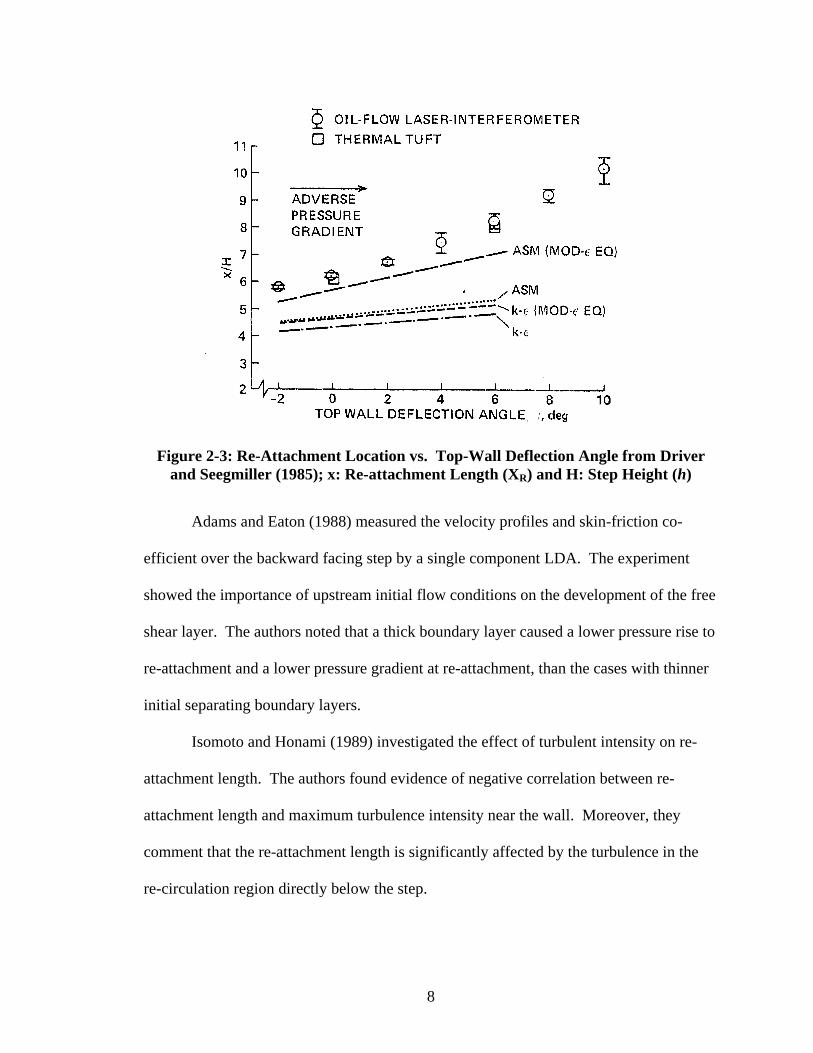
Driver and Seegmiller (1985) analyzed the effect of pressure gradient on re-
attachment length of turbulent flow over a backward facing step. They varied the
pressure gradient by changing the angle of the top-wall with the horizontal while velocity
measurements were carried out with Laser Doppler Anemometer (LDA). The authors
found an increase in reattachment length with top-wall angle. They also compared the
numerical predictions with the experimental results and found that the numerical results
under-predict the reattachment length. Their results can be observed from Figure 2-3.
8
Figure 2-3: Re-Attachment Location vs. Top-Wall Deflection Angle from Driver and Seegmiller (1985); x: Re-attachment Length (XR) and H: Step Height (h)
Adams and Eaton (1988) measured the velocity profiles and skin-friction co-
efficient over the backward facing step by a single component LDA. The experiment
showed the importance of upstream initial flow conditions on the development of the free
shear layer. The authors noted that a thick boundary layer caused a lower pressure rise to
re-attachment and a lower pressure gradient at re-attachment, than the cases with thinner
initial separating boundary layers.
Isomoto and Honami (1989) investigated the effect of turbulent intensity on re-
attachment length. The authors found evidence of negative correlation between re-
attachment length and maximum turbulence intensity near the wall. Moreover, they
comment that the re-attachment length is significantly affected by the turbulence in the
re-circulation region directly below the step.
9
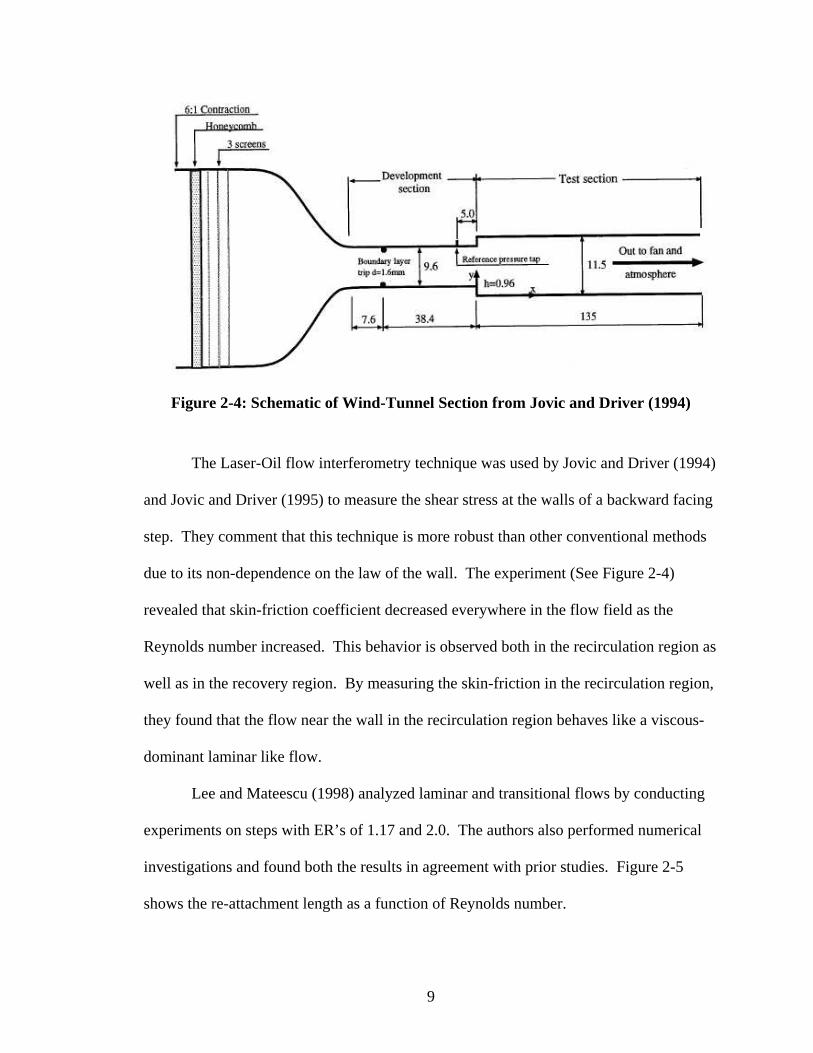
Figure 2-4: Schematic of Wind-Tunnel Section from Jovic and Driver (1994)
The Laser-Oil flow interferometry technique was used by Jovic and Driver (1994)
and Jovic and Driver (1995) to measure the shear stress at the walls of a backward facing
step. They comment that this technique is more robust than other conventional methods
due to its non-dependence on the law of the wall. The experiment (See Figure 2-4)
revealed that skin-friction coefficient decreased everywhere in the flow field as the
Reynolds number increased. This behavior is observed both in the recirculation region as
well as in the recovery region. By measuring the skin-friction in the recirculation region,
they found that the flow near the wall in the recirculation region behaves like a viscous-
dominant laminar like flow.
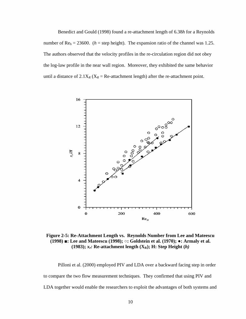
Lee and Mateescu (1998) analyzed laminar and transitional flows by conducting
experiments on steps with ER’s of 1.17 and 2.0. The authors also performed numerical
investigations and found both the results in agreement with prior studies. Figure 2-5
shows the re-attachment length as a function of Reynolds number.
10
Benedict and Gould (1998) found a re-attachment length of 6.38h for a Reynolds
number of Reh = 23600. (h = step height). The expansion ratio of the channel was 1.25.
The authors observed that the velocity profiles in the re-circulation region did not obey
the log-law profile in the near wall region. Moreover, they exhibited the same behavior
until a distance of 2.1XR (XR = Re-attachment length) after the re-attachment point.
Figure 2-5: Re-Attachment Length vs. Reynolds Number from Lee and Mateescu (1998) ■: Lee and Mateescu (1998); ○: Goldstein et al. (1970); ●: Armaly et al.
(1983); xr: Re-attachment length (XR); H: Step Height (h)
Pilloni et al. (2000) employed PIV and LDA over a backward facing step in order
to compare the two flow measurement techniques. They confirmed that using PIV and
LDA together would enable the researchers to exploit the advantages of both systems and
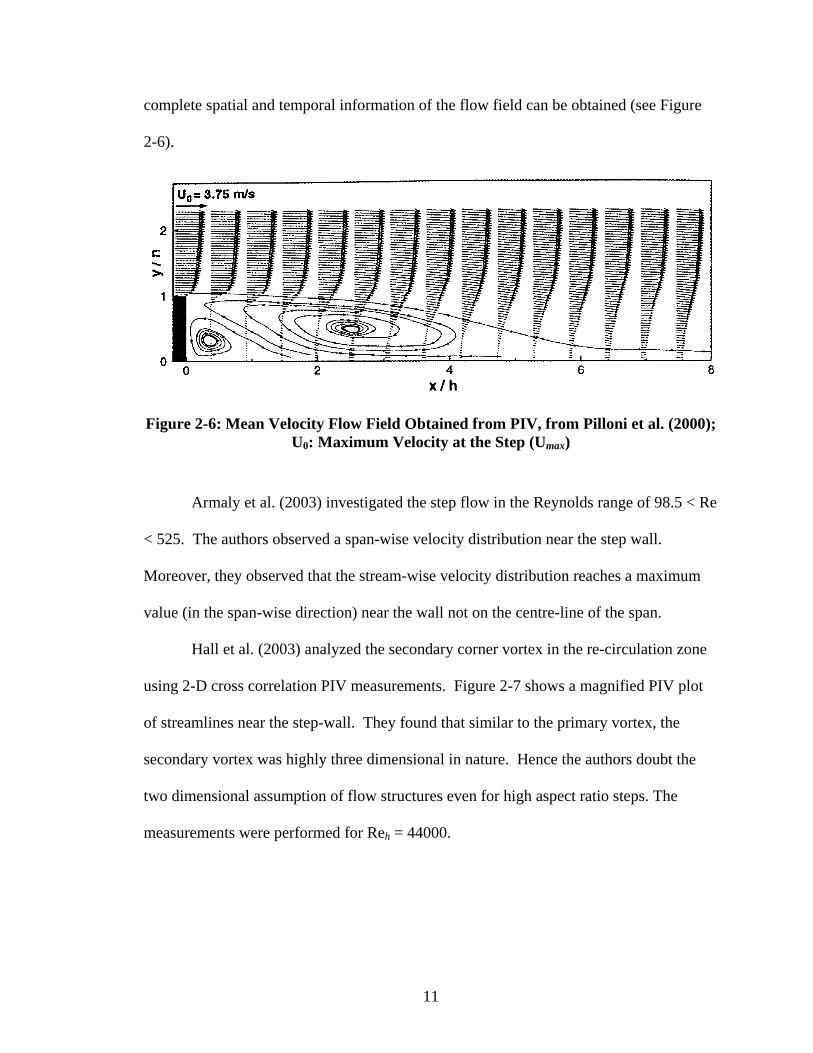
11
complete spatial and temporal information of the flow field can be obtained (see Figure
2-6).
Figure 2-6: Mean Velocity Flow Field Obtained from PIV, from Pilloni et al. (2000); U0: Maximum Velocity at the Step (Umax)
Armaly et al. (2003) investigated the step flow in the Reynolds range of 98.5 < Re
< 525. The authors observed a span-wise velocity distribution near the step wall.
Moreover, they observed that the stream-wise velocity distribution reaches a maximum
value (in the span-wise direction) near the wall not on the centre-line of the span.
Hall et al. (2003) analyzed the secondary corner vortex in the re-circulation zone
using 2-D cross correlation PIV measurements. Figure 2-7 shows a magnified PIV plot
of streamlines near the step-wall. They found that similar to the primary vortex, the
secondary vortex was highly three dimensional in nature. Hence the authors doubt the
two dimensional assumption of flow structures even for high aspect ratio steps. The
measurements were performed for Reh = 44000.
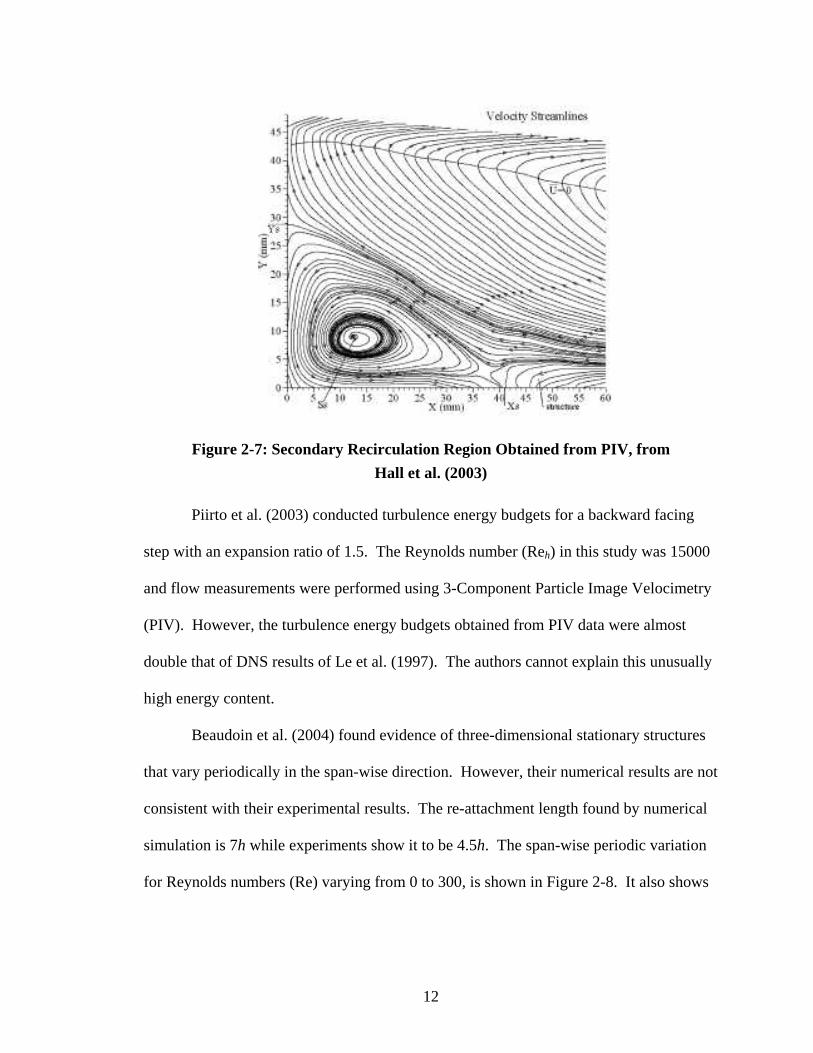
12
Figure 2-7: Secondary Recirculation Region Obtained from PIV, from
Hall et al. (2003)
Piirto et al. (2003) conducted turbulence energy budgets for a backward facing
step with an expansion ratio of 1.5. The Reynolds number (Reh) in this study was 15000
and flow measurements were performed using 3-Component Particle Image Velocimetry
(PIV). However, the turbulence energy budgets obtained from PIV data were almost
double that of DNS results of Le et al. (1997). The authors cannot explain this unusually
high energy content.
Beaudoin et al. (2004) found evidence of three-dimensional stationary structures
that vary periodically in the span-wise direction. However, their numerical results are not
consistent with their experimental results. The re-attachment length found by numerical
simulation is 7h while experiments show it to be 4.5h. The span-wise periodic variation
for Reynolds numbers (Re) varying from 0 to 300, is shown in Figure 2-8. It also shows
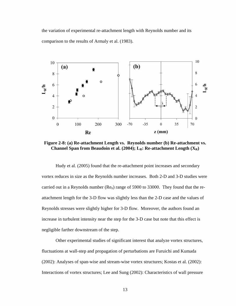
13
the variation of experimental re-attachment length with Reynolds number and its
comparison to the results of Armaly et al. (1983).
Figure 2-8: (a) Re-attachment Length vs. Reynolds number (b) Re-attachment vs. Channel Span from Beaudoin et al. (2004); LR: Re-attachment Length (XR)
Hudy et al. (2005) found that the re-attachment point increases and secondary
vortex reduces in size as the Reynolds number increases. Both 2-D and 3-D studies were
carried out in a Reynolds number (Reh) range of 5900 to 33000. They found that the re-
attachment length for the 3-D flow was slightly less than the 2-D case and the values of
Reynolds stresses were slightly higher for 3-D flow. Moreover, the authors found an
increase in turbulent intensity near the step for the 3-D case but note that this effect is
negligible farther downstream of the step.
Other experimental studies of significant interest that analyze vortex structures,
fluctuations at wall-step and propagation of perturbations are Furuichi and Kumada
(2002): Analyses of span-wise and stream-wise vortex structures; Kostas et al. (2002):
Interactions of vortex structures; Lee and Sung (2002): Characteristics of wall pressure
14
fluctuations; Furuichi et al. (2004): large-scale structures and fluctuations at wall step;
Lee et al. (2004): Large scale vortical structures; Camussi et al. (2006): Wall pressure
perturbations propagation at low Reynolds number; and Ke et al. (2005): Flow with and
without entrainment and large-scale structures.
2.3 Numerical Studies on Backward Facing Steps
As noted by Yang et al. (2003), the reattachment point is a critical parameter that
usually determines the accuracy and performance of any numerical model. Hence, the
experimental data of Armaly et al. (1983), Jovic and Driver (1994), Driver and
Seegmiller (1985), Lee and Mateescu (1998) etc. are used extensively by researchers to
validate their numerical studies. There are numerous 2-D and 3-D analyses of the
backward facing step. This is justified, as Stephano et al. (1998) notes that every time a
new numerical method is developed, it is applied and examined on backward facing step
geometry to test its accuracy. A model that fails to predict the reattachment length past a
backward facing step could never calculate the reattachment in complex engineering
turbulent flows. This section of the review discusses the numerical studies on backward
facing step geometries that include (a) 2-D and 3-D Laminar Flow Analysis, (b) Direct
Numerical Simulation (DNS), (c) Large Eddy Simulation (LES) and (d) Detached Eddy
Simulation (DES).
2.3.1 Laminar Flow Analyses: 2D and 3D
Early numerical simulations of the step were restricted to the two-dimensional
analysis primarily due to the lack of computer power. Armaly et al. (1983) conducted a
15
numerical analysis and found that the results matched quite well with the experimental
results up to Re ≈ 400. They hypothesized that the presence of secondary recirculation
zone was the cause of the discrepancy between the experimental and numerical solutions.
Other significant numerical studies of that period that discuss the 2-D numerical analysis
over the step were Goussibaile et al. (1984), Toumi et al. (1984), Ecer et al. (1984) and
Braza et al. (1984). It is useful to note that all the above papers use finite difference
method for the numerical analysis.
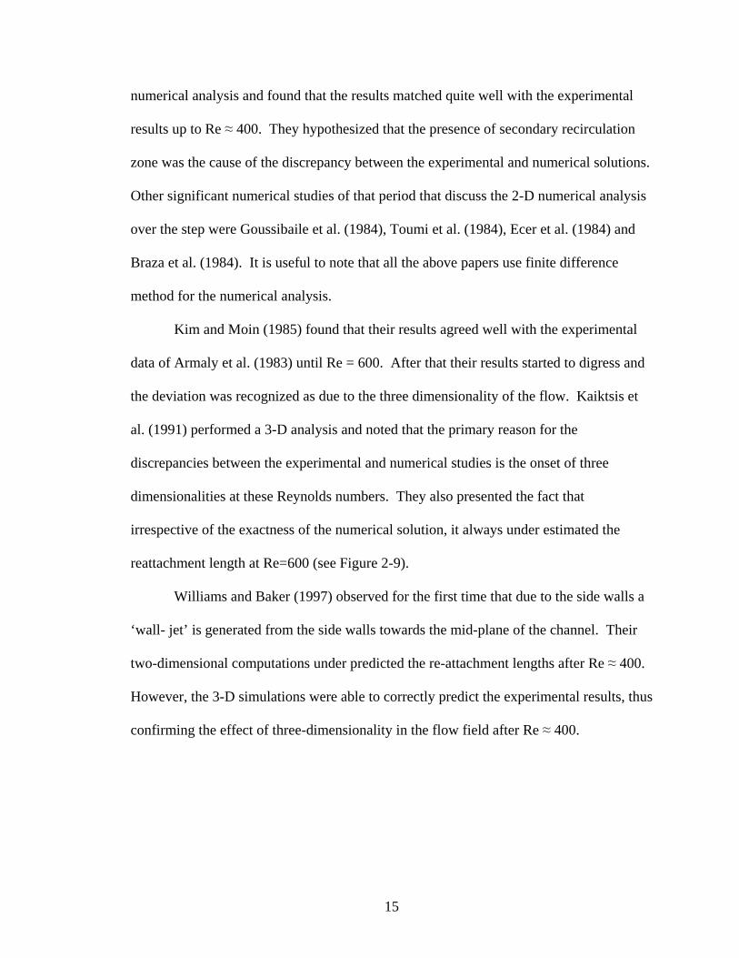
Kim and Moin (1985) found that their results agreed well with the experimental
data of Armaly et al. (1983) until Re = 600. After that their results started to digress and
the deviation was recognized as due to the three dimensionality of the flow. Kaiktsis et
al. (1991) performed a 3-D analysis and noted that the primary reason for the
discrepancies between the experimental and numerical studies is the onset of three
dimensionalities at these Reynolds numbers. They also presented the fact that
irrespective of the exactness of the numerical solution, it always under estimated the
reattachment length at Re=600 (see Figure 2-9).
Williams and Baker (1997) observed for the first time that due to the side walls a
‘wall- jet’ is generated from the side walls towards the mid-plane of the channel. Their
two-dimensional computations under predicted the re-attachment lengths after Re ≈ 400.
However, the 3-D simulations were able to correctly predict the experimental results, thus
confirming the effect of three-dimensionality in the flow field after Re ≈ 400.
16
.
Figure 2-9: Re-Attachment Length vs. Reynolds number for Laminar Flow from Kim and Moin (1985); xr: Re-attachment length (XR)
Chiang and Sheu (1998) conducted extensive 3-D analysis in the Reynolds
number range of 100 < Re < 1000 and found that two dimensionality in the flow is
achieved at Re = 800 only when the channel width is almost 100 times the step height.
Their results showed excellent agreement with the experiments of Armaly et al. (1983)
for Re between 100 and 389. They applied topology theory to the numerical analysis and
studied the complex vortical flow structure in explicit detail. Similar experimental and
numerical results were obtained by Tylii et al. (2002)
Biswas et al. (2004) presented a review of previous studies and also conducted
numerical investigations on backward-facing step flows with expansion ratios of 1.9423,
2.5 and 3.0. Their investigation of step flows (0.0001 < Re < 800) yielded results akin to
Williams and Baker (1997) and Chiang and Sheu (1998). Moreover, the authors also
17
evaluated pressure losses for various expansion ratios and found that the losses decreased
with an increase in Reynolds number and decrease in step-height.
Gualtieri (2005) investigated 2-D step-flow using commercial software
FEMLAB. The simulations were performed for a Reynolds number range of 84 to 1006.
Their results indicated that beyond Re = 300, the re-attachment length was under
predicted by FEMLAB software.
Kanna and Das (2006) analyzed the backward facing step flow using the stream-
function – vorticity approach. They found that at Re= 800, even though good agreement
was observed for the u-velocity after re-attachment, considerable disagreements were
found in the v-velocity. The authors comment that these discrepancies contribute directly
to the measurement accuracy of the re-attachment of primary vortex.
2.3.2 Direct Numerical Simulation (DNS)
The Navier-Stokes (N-S) equation correctly describes both the laminar and the
turbulent flows of a Newtonian fluid. One of the most powerful techniques to be
developed to solve the N-S equations is undoubtedly the Direct Numerical Simulation
(DNS). But unfortunately, this technique is extremely expensive and the computational
cost increases as the order of Re3. Moreover, most of the effort (almost 99.8 %) is used
to simulate the flow in the dissipation scales (Pope, 2000). These smaller scales can
obviously be modeled, while the large scales can still be simulated. This is the basis of
the technique: Large Eddy Simulation (LES). LES can save considerable amount of
computational time as compared to DNS but even LES has not evolved enough to find its
way as a practical engineering tool. The working engineer still relies on the traditional
18
approach of Reynolds-averaged-Navier-Stokes (RANS) equation for the solution. The
various models of RANS equation i.e. the k-ε models will be discussed later in the
section.
One of the most comprehensive analyses of the backward facing step was the
Direct Numerical Simulation (DNS) carried out by Le et al. (1997). The Reynolds
number (based on step height and inlet velocity) at which the computations were done is
5100. The grids used were 768, 192 and 64 in the x, y and z directions respectively.
They found that the re-attachment point varied in the span wise direction and it oscillated
about a mean value of 6.28 S. Their results are in excellent agreement with the
experimental data of Jovic and Driver (1994). Their extensive analysis contains up to
third order statistics and Reynolds stress budgets at every location in the flow field. The
DNS for the first time reported (a) the presence of a large negative skin friction in the
recirculation region at relatively low Re (which agreed with the experimental readings)
and (b) deviation of the velocity profile from the log law in the recovery region. This
indicates that the flow is not fully recovered even at twenty step heights behind the step.
Valsecchi (2005) conducted DNS for transitional flow over a backward facing
step for Re = 3000 and an expansion ratio of 1.09. They found that the DNS results were
in good agreement with the experimental results. Other applications of DNS to simulate
a passive control method (thereby reducing the reattachment length) were studied by
Neumann and Wengle (2003). They found that a certain minimum distance between the
step edge and control fence (a small obstruction upstream of the step that causes the flow
to be turbulent) is required to achieve maximum reduction of reattachment length. Other
19
significant studies that analyze periodically perturbed flow using LES and DNS are
Dejoan et al. (2005) and Saric et al. (2005).
2.3.3 Large Eddy Simulation (LES)
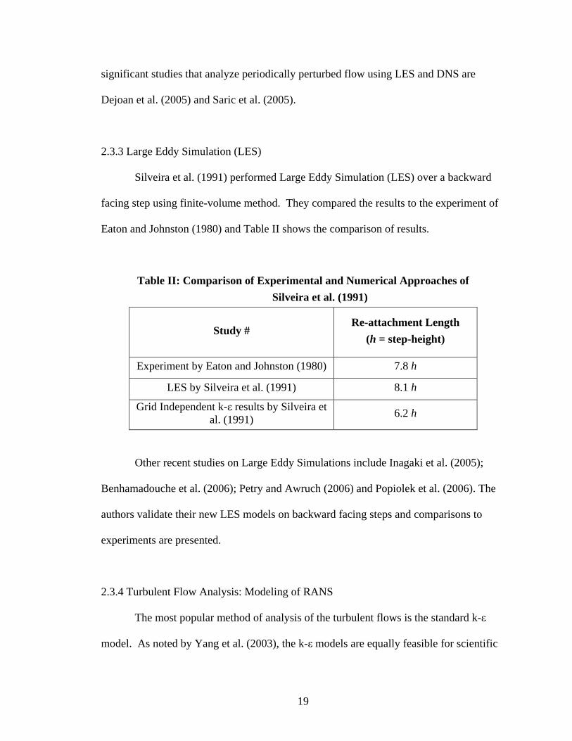
Silveira et al. (1991) performed Large Eddy Simulation (LES) over a backward
facing step using finite-volume method. They compared the results to the experiment of
Eaton and Johnston (1980) and Table II shows the comparison of results.
Table II: Comparison of Experimental and Numerical Approaches of
Silveira et al. (1991)
Study # Re-attachment Length
(h = step-height)
Experiment by Eaton and Johnston (1980) 7.8 h
LES by Silveira et al. (1991) 8.1 h
Grid Independent k-ε results by Silveira et al. (1991)
6.2 h
Other recent studies on Large Eddy Simulations include Inagaki et al. (2005);
Benhamadouche et al. (2006); Petry and Awruch (2006) and Popiolek et al. (2006). The
authors validate their new LES models on backward facing steps and comparisons to
experiments are presented.
2.3.4 Turbulent Flow Analysis: Modeling of RANS
The most popular method of analysis of the turbulent flows is the standard k-ε
model. As noted by Yang et al. (2003), the k-ε models are equally feasible for scientific
20
research as well as for engineering applications of complex turbulent flows. The
turbulent flow models can be classified as (a) linear models and (b) non-linear models.
Two of the linear models are the standard k-ε model of Launder and Spalding (1974) and
the non-equilibrium model of Yoshizawa and Nisizima (1993).
As noted by Pope (2000), the standard k-ε model is not able to capture the
secondary turbulent flows in a duct with non-circular cross-section. As a result,
important non-linear models were formulated primarily to overcome this deficiency of
the standard k-ε model. Quadratic models include those developed by Speziale (1987)
and Shih, Zhu and Lumley (1995), while an example of a cubic model is the one
developed by Craft, Launder and Suga (1996). Yang et al. (2003) compare all the linear
and non-linear models mentioned above and observe that all the models under-predict the
reattachment length. They also find that the non-linear models of Shih, Zhu and Lumley
(1995) and Craft, Launder and Suga (1996) perform better than the linear models, and are
closer to the experimental value of re-attachment length.
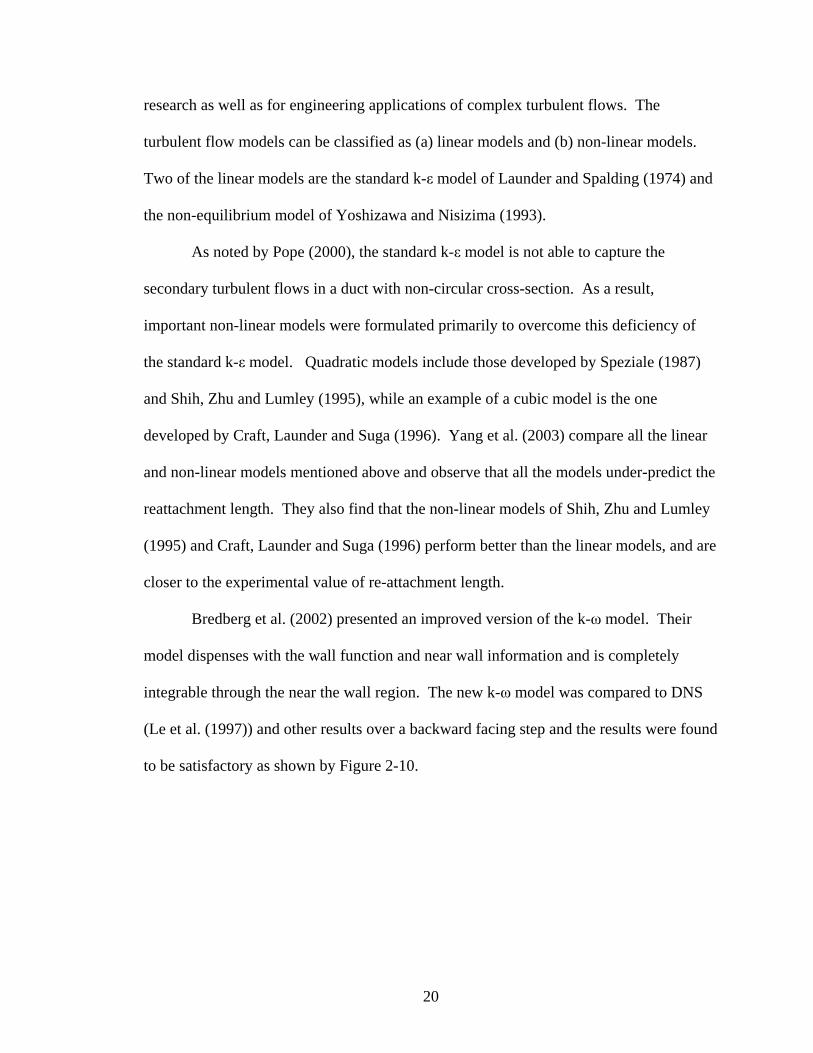
Bredberg et al. (2002) presented an improved version of the k-ω model. Their
model dispenses with the wall function and near wall information and is completely
integrable through the near the wall region. The new k-ω model was compared to DNS
(Le et al. (1997)) and other results over a backward facing step and the results were found
to be satisfactory as shown by Figure 2-10.
21
Figure 2-10: Skin Friction Co-efficient vs. x/h from Bredberg et al. (2002)
Kim et al. (2005) simulated the experiment of Driver and Seegmiller (1985) using
commercial software FLUENT. Their study confirmed that different combinations of
turbulence models and wall treatment methods resulted in varying re-attachment lengths.
Celik and Li (2005) presented a numerical uncertainty analyses on turbulent flow
simulations over a backward facing step using FLUENT software. The authors
concluded that four sets of carefully selected grids were adequate for uncertainty analysis
and grid convergence.
2.4 Experimental Studies on Porous Media
In this section of the literature review, recent advances in turbulent flow modeling
in porous media are presented. Two distinct sets of modeling approaches can be
observed from the literature depending on the order of integration i.e. starting with space-
averaging (space-time approach) or starting with time-averaging (time-space approach).
22
These methodologies are reviewed in detail and the various models with different
complexities are discussed. Moreover, conclusions are presented with regards to their
accuracy and flexibility of application.
The flow in porous media has been generally considered laminar due to the
relatively small pore size. However, experimenters did find instances of chaotic or
turbulent flow in porous media. In the literature one finds only a handful of experiments
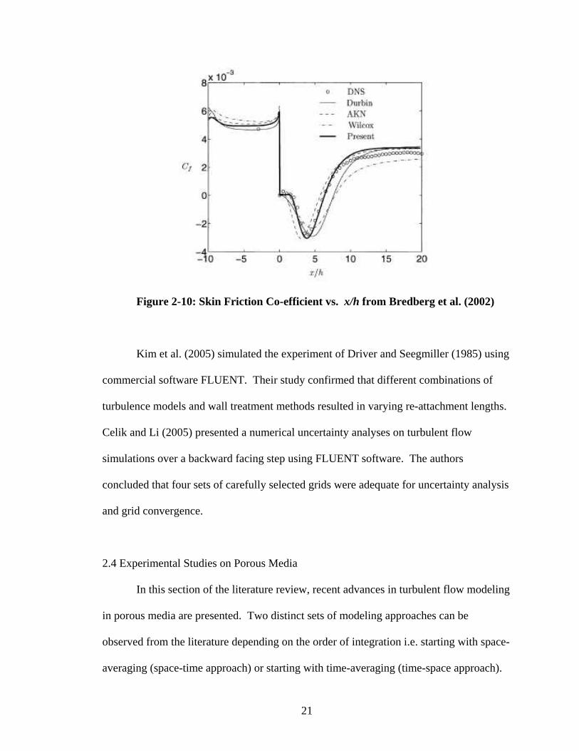
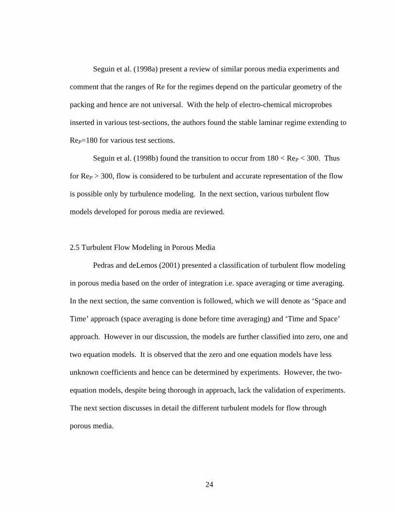
on turbulent flows in porous media. Dybbs and Edwards (1984) studied the flow of water
and various oils through a fixed three dimensional packing of Plexiglas spheres and
cylinders, shown in Figure 2-11. Laser anemometry and flow visualization revealed four
distinct flow regimes as summarized in Table III. Here, ReP is the pore Reynolds number
which is defined as the Reynolds number based on the pore size and ReP is given by
Equation 2.1.
µρ PP
P
dU=Re (2.1)
(where ρ: fluid density, µ: fluid viscosity, UP: pore velocity and dP: pore diameter)
In the Darcy or Creeping flow regime, viscous forces dominate the flow and
Darcy’s equation (Equation 2.2) governs the flow. In this region relationship between the
pressure drop and flow rate is linear. From Re = 1 to 10, the authors observed the
formation of a boundary layer on the solid surfaces of the porous media and an inertial
core. The pressure drop-flow rate relation turns non-linear in this region. This continues
until Re = 150 which is characterized by steady laminar flow and unsteady flow persists
until Re = 300. The Reynolds number investigated in this study ranged from 0.16 to 700.
23
bvCvp
+−=∆ 22 2
1 ραµ (2.2)
(where α: permeability, C2: inertial constant, v: velocity and b: filter thickness)
Table III: Flow Regimes in Porous Media Summarized from Experiment by
Dybbs and Edwards (1984)
Figure 2-11: Cross section of Porous Medium Packed Bed of Spheres,
from Dybbs and Edwards (1984)
Range of ReP Regime
ReP < 1 Darcy or Creeping Flow
1< ReP < 10 Inertial Flow
1 < ReP < 150 Steady Laminar Flow
150 < ReP < 300 Unsteady Laminar Flow
ReP > 300 Turbulent Flow
24
Seguin et al. (1998a) present a review of similar porous media experiments and
comment that the ranges of Re for the regimes depend on the particular geometry of the
packing and hence are not universal. With the help of electro-chemical microprobes
inserted in various test-sections, the authors found the stable laminar regime extending to
ReP=180 for various test sections.
Seguin et al. (1998b) found the transition to occur from 180 < ReP < 300. Thus
for ReP > 300, flow is considered to be turbulent and accurate representation of the flow
is possible only by turbulence modeling. In the next section, various turbulent flow
models developed for porous media are reviewed.
2.5 Turbulent Flow Modeling in Porous Media
Pedras and deLemos (2001) presented a classification of turbulent flow modeling
in porous media based on the order of integration i.e. space averaging or time averaging.
In the next section, the same convention is followed, which we will denote as ‘Space and
Time’ approach (space averaging is done before time averaging) and ‘Time and Space’
approach. However in our discussion, the models are further classified into zero, one and
two equation models. It is observed that the zero and one equation models have less
unknown coefficients and hence can be determined by experiments. However, the two-
equation models, despite being thorough in approach, lack the validation of experiments.
The next section discusses in detail the different turbulent models for flow through
porous media.
25
2.5.1 Space and Time Approach
1. Two Equation k-ε Models: Lee and Howell (1987) proposed a simplified
version of the standard k-ε model to analyze fluid flow in porous media. Their model
was one of the first efforts to model turbulent flow in porous media and hence considers a
lot of assumptions that simplifies the analysis to a great extent. Forchheimer’s resistance
term is considered in their modified Darcy’s equation but they do not include the
Brinkman’s term that reflects the viscous diffusion effects (See Equation 3.8). The
momentum equations are considered for both the homogenous fluid flow and the flow
through porous media. The partial differential equations for k (turbulent kinetic energy)
and ε (turbulent dissipation) are derived from the momentum equations by assuming that
the absolute value of the velocity does not depend on the turbulent flow. The Navier-
Stokes equations are not time-averaged and hence the model doesn’t account for the
Reynolds stresses caused by the turbulence. However, they consider the effective
viscosity as an algebraic sum of molecular viscosity and an eddy viscosity. This effective
viscosity is considered in the calculation of the viscous diffusion term. The value of
coefficients used for modeling in porous media is the same as used for plain fluid flow.
Antohe and Lage (1997) developed a k-ε model in which all the terms of the
extended Darcy’s equation are present. Time averaging of Navier-Stokes equation was
done to obtain momentum equations and the closure was obtained by modeling the
Reynolds stresses by solving PDE’s (Partial differential equations) for k and ε. Due to
the time-averaging process, their analyses are more complex than Lee and Howell (1987)
and leads to extra terms from Darcy and Forchheimer’s in the equations of k and ε. Their
26
derivation results in the conclusion that the Darcy’s term damps the flow while the effect
of Forchheimer’s term on k is inconclusive. They also suggest separate sets of equations
(with extra terms) for application at low Reynolds numbers. It is interesting to observe
that the value of the coefficients used in the equations is the same as that for pure fluid at
low Reynolds numbers. This is due to the lack of experimental data for turbulent flow
through porous media. They presume that these constants may be a function of porosity
at lower porosities.
Antohe and Lage (1997) found that for a steady one-dimensional fully developed
flow, macroscopic turbulence cannot sustain in a porous medium i.e. they found that the
only solution for this case is k = 0 and ε = 0. This is the main disadvantage of the model.
This is attributed to the exclusion of microscopic turbulent quantities in the determination
of macroscopic quantities due to the space-averaging of the equations before the time-
averaging process. This is because, during space averaging of the microscopic
fluctuations of any quantity, the smoothing of macroscopic results takes place. Further
time-averaging simply results in excluding the effect of these fluctuations on the
macroscopic quantity. This drawback has brought forward the issue that the order of
time-averaging and space-averaging may be important and is further explained in the
models of Pedras and deLemos (2001).
Getachew et al. (2000) presented a revised version of k-ε model proposed by
Antohe and Lage (1997). The primary difference between the two approaches being the
use of a second-order correlation term in the Forchheimer’s resistance term in the time-
averaged momentum equation. The main effect due to this modification stems from the
fact that these terms give rise to additional coefficients that are able to reflect the

27
microscopic turbulence effects in a better manner. The authors believe that representing
Forchheimer’s term as higher order correlation terms will avoid excluding vital effects of
turbulent flow in porous media. As discussed above, these additional terms appear in the
differential equations for k as third-order moments (or triple velocity correlations). These
are modeled by using techniques similar to Hanjalic and Launder (1992) (cited from
Getachew et al. (2000)).This model is more precise than the one by Antohe and Lage
(1997) for the case when the kinetic energy is much greater than the dissipation. The
dissipation equation also turns out have additional unknown double and triple moments
of various quantities. In general, the authors choose to model these unknowns in terms of
mean velocity gradients, Reynolds stresses and dissipation. The authors also note that
there are several new undetermined coefficients that can be found only by experiments on
turbulent flow in porous media. Similar to the procedure adopted by previous
investigators of turbulent flow modeling in porous media, the present authors are forced
to adopt the coefficients for the limiting case of α→ ∞ and φ = 1, which are the
conditions for pure homogenous fluid flow.
2. RNG model: Avramenko and Kuznetsov (2006) proposed a RNG
(renormalization group) model for flow through porous media. Their methodology is
similar to that of Antohe and Lage (1997), in the sense that their model does not reflect
the microscopic fluctuations in the macroscopic equations. However, they use the RNG
approach (developed by Yakhot and Orszag (1986)) while Antohe and Lage (1997) use
the time-averaging procedure. Their results confirm that the porous media decreases the
28
velocity and flattens the velocity profile. The closure is obtained by using the mixing
length model of turbulence.
2.5.2 Time and Space Approach
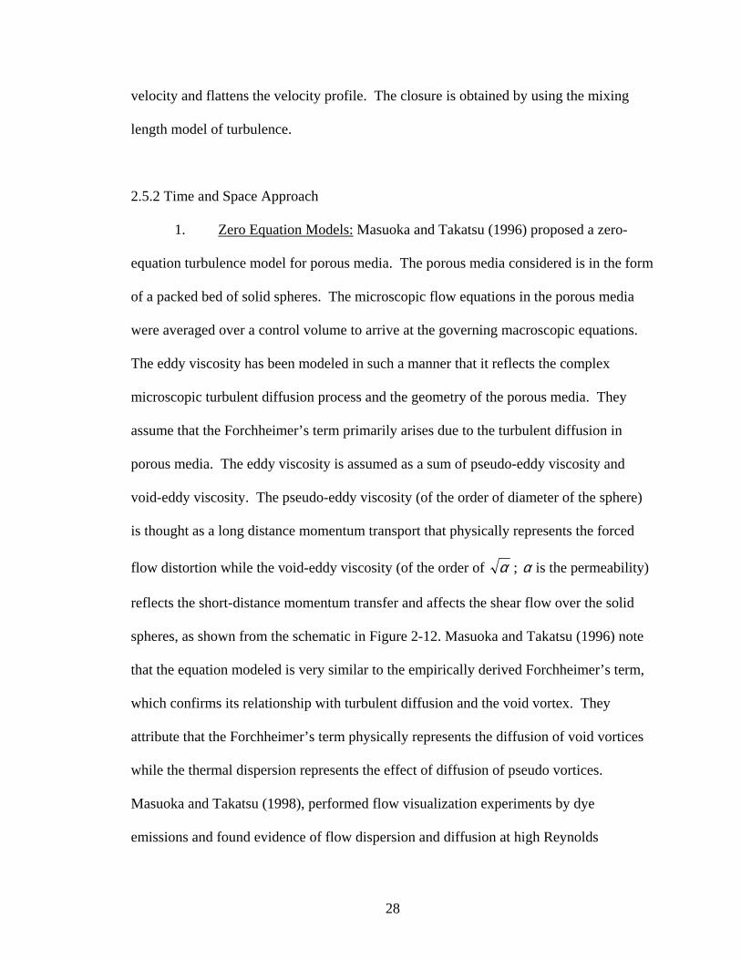
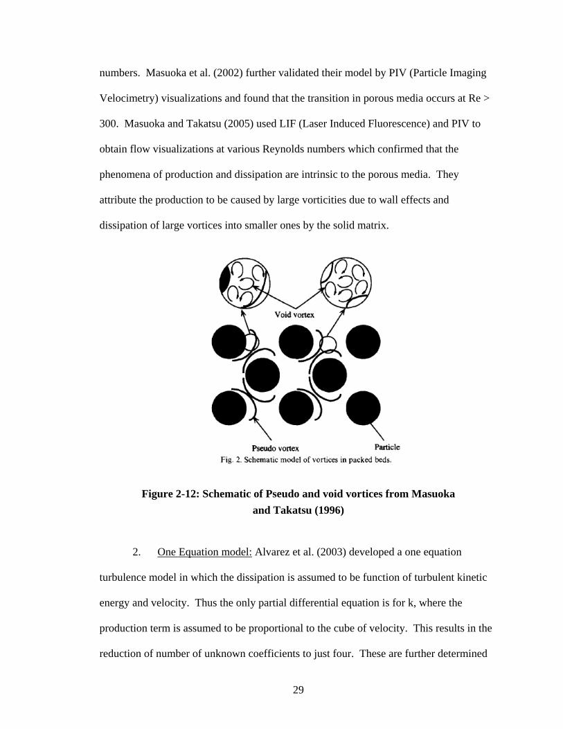
1. Zero Equation Models: Masuoka and Takatsu (1996) proposed a zero-
equation turbulence model for porous media. The porous media considered is in the form
of a packed bed of solid spheres. The microscopic flow equations in the porous media
were averaged over a control volume to arrive at the governing macroscopic equations.
The eddy viscosity has been modeled in such a manner that it reflects the complex
microscopic turbulent diffusion process and the geometry of the porous media. They
assume that the Forchheimer’s term primarily arises due to the turbulent diffusion in
porous media. The eddy viscosity is assumed as a sum of pseudo-eddy viscosity and
void-eddy viscosity. The pseudo-eddy viscosity (of the order of diameter of the sphere)
is thought as a long distance momentum transport that physically represents the forced
flow distortion while the void-eddy viscosity (of the order of α ; α is the permeability)
reflects the short-distance momentum transfer and affects the shear flow over the solid
spheres, as shown from the schematic in Figure 2-12. Masuoka and Takatsu (1996) note
that the equation modeled is very similar to the empirically derived Forchheimer’s term,
which confirms its relationship with turbulent diffusion and the void vortex. They
attribute that the Forchheimer’s term physically represents the diffusion of void vortices
while the thermal dispersion represents the effect of diffusion of pseudo vortices.
Masuoka and Takatsu (1998), performed flow visualization experiments by dye
emissions and found evidence of flow dispersion and diffusion at high Reynolds
29
numbers. Masuoka et al. (2002) further validated their model by PIV (Particle Imaging
Velocimetry) visualizations and found that the transition in porous media occurs at Re >
300. Masuoka and Takatsu (2005) used LIF (Laser Induced Fluorescence) and PIV to
obtain flow visualizations at various Reynolds numbers which confirmed that the
phenomena of production and dissipation are intrinsic to the porous media. They
attribute the production to be caused by large vorticities due to wall effects and
dissipation of large vortices into smaller ones by the solid matrix.
Figure 2-12: Schematic of Pseudo and void vortices from Masuoka
and Takatsu (1996)
2. One Equation model: Alvarez et al. (2003) developed a one equation
turbulence model in which the dissipation is assumed to be function of turbulent kinetic
energy and velocity. Thus the only partial differential equation is for k, where the
production term is assumed to be proportional to the cube of velocity. This results in the
reduction of number of unknown coefficients to just four. These are further determined
30
by experimental investigation of airflow through PVC spheres. This semi-empirical one
equation model compares well for experimental fluid flow and heat transfer results
primarily due to the values obtained for the coefficients.
3. Two Equation Models: The two equation models have been the most
popular approach in the literature owing to their capability to model intricate features of
the turbulent flows. In order to find the value of undetermined coefficient (Cε) that
appears in the differential equation for ε, Chung et al. (2003) performed experiments on a
channel with micro-tubes. Microscopic experimental analysis of the fluid flow (Friction
Factor) and heat transfer (Nusselt Number) were conducted and the authors found that for
a Cε value of 0.99, the friction factors and Nusselt numbers obtained numerically
matched well with the experimental results. A modified form of the equations is
presented which overcome the numerical deficiency highlighted by the model of Antohe
and Lage (1997). This shortcoming is overcome by representing the source term as two
different terms, one each for homogenous flow and flow in porous media. For conditions
of high permeability and high porosity (α→ ∞ and φ = 1) i.e. for homogeneous fluid, the
porous media source term automatically vanishes and a mathematical solution is
obtained. The authors go on to prove that the value of the constant is independent of the
Reynolds numbers and porosity. However, the authors have assumed local thermal
equilibrium conditions and hence the model cannot be extended to inlet regions and non-
uniform porous media.
Pedras and deLemos (2001) developed a two-equation turbulence model in which
the undetermined constant is proposed by numerical solution of structured porous media
31
in the form of an infinite array of circular rods. The authors confirm that the solution of
macroscopic momentum equations is independent of the order of integration. (Space
averaging and time averaging). However, the turbulent kinetic energy depends
considerably on the order of integration. In the present analysis, local time average is
considered first and then the space-average is taken. This approach is the reverse of the
methodologies of Antohe and Lage (1997) and Lee and Howell (1987). The value of the
constant was found to be 0.28 and the macroscopic data for turbulent kinetic energy and
dissipation matched well with the values from Nakayama and Kuwahara (1999). The
slight difference between the two data is attributed to the fact that Nakayama and
Kuwahara (1999) used an array of square cross-section rods.
Pedras and deLemos (2003) tested the model coefficient on arrays of transversely
and longitudinally elliptical rods and found that it is reasonable to assume the same value
for the constant in the k-equation irrespective of the porous media geometry. Their
results were in close agreement to circular and square cross sections results from the
literature.
Chandesris et al. (2006) developed a macroscopic turbulence model in which the
core of a nuclear reactor is modeled as a porous media due to similarities in the two
geometries. Thus, this model serves to simulate flows in pipes, channels and rod-
bundles. The unknown coefficients that arise from the modeling expressions are obtained
from microscopic equations which are validated against the existing experimental and
DNS (Direct Numerical Simulation) data for channel flows, pipe flows, arrays of square
rods and circular rods. The authors use the same model for macroscopic turbulent
viscosity as used by Pedras and deLemos (2001) and Nakayama and Kuwahara (1999).
32
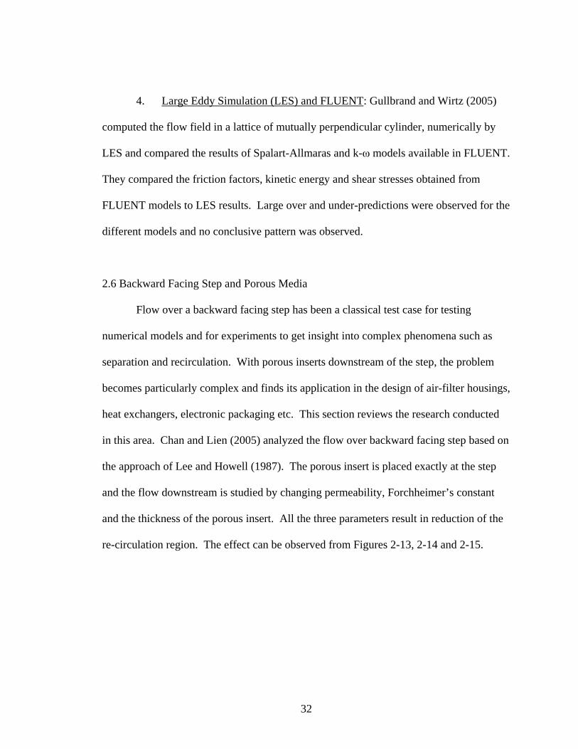
4. Large Eddy Simulation (LES) and FLUENT: Gullbrand and Wirtz (2005)
computed the flow field in a lattice of mutually perpendicular cylinder, numerically by
LES and compared the results of Spalart-Allmaras and k-ω models available in FLUENT.
They compared the friction factors, kinetic energy and shear stresses obtained from
FLUENT models to LES results. Large over and under-predictions were observed for the
different models and no conclusive pattern was observed.
2.6 Backward Facing Step and Porous Media
Flow over a backward facing step has been a classical test case for testing
numerical models and for experiments to get insight into complex phenomena such as
separation and recirculation. With porous inserts downstream of the step, the problem
becomes particularly complex and finds its application in the design of air-filter housings,
heat exchangers, electronic packaging etc. This section reviews the research conducted
in this area. Chan and Lien (2005) analyzed the flow over backward facing step based on
the approach of Lee and Howell (1987). The porous insert is placed exactly at the step
and the flow downstream is studied by changing permeability, Forchheimer’s constant
and the thickness of the porous insert. All the three parameters result in reduction of the
re-circulation region. The effect can be observed from Figures 2-13, 2-14 and 2-15.
33
Figure 2-13: Sensitivity of flow field (stream-traces) to changes in Darcy number for
b/h = 0:3 and F = 0:55 from Chan and Lien (2005)
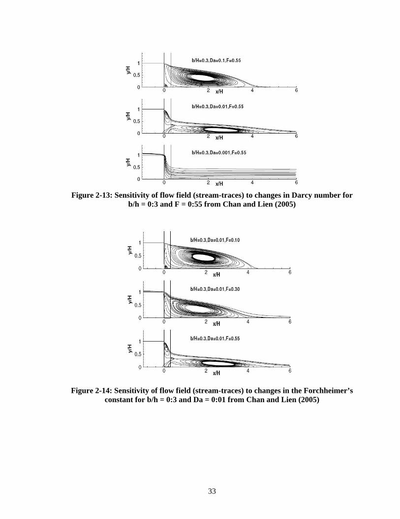
Figure 2-14: Sensitivity of flow field (stream-traces) to changes in the Forchheimer’s constant for b/h = 0:3 and Da = 0:01 from Chan and Lien (2005)
34
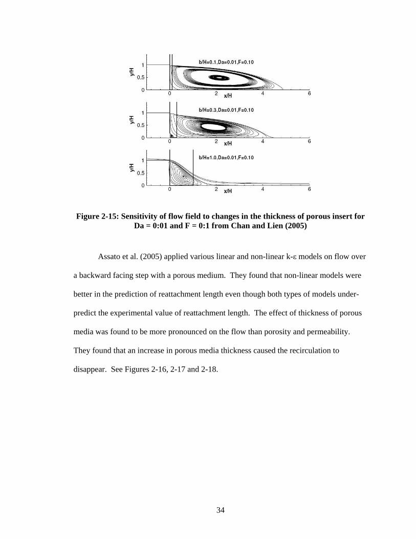
Figure 2-15: Sensitivity of flow field to changes in the thickness of porous insert for Da = 0:01 and F = 0:1 from Chan and Lien (2005)
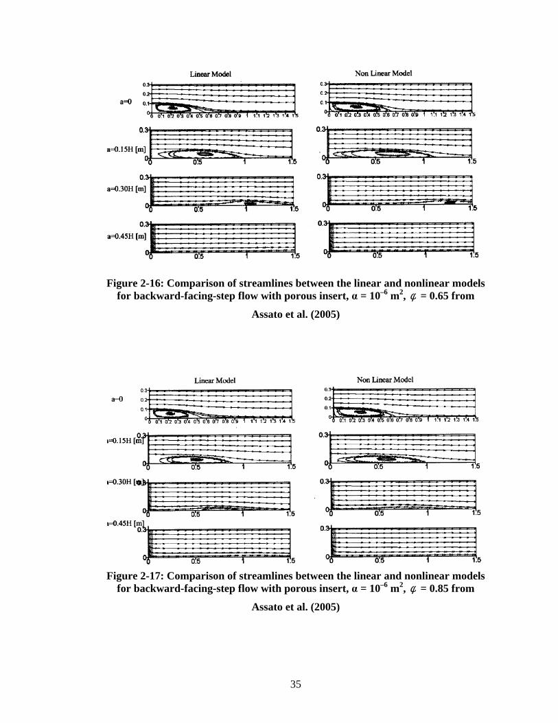
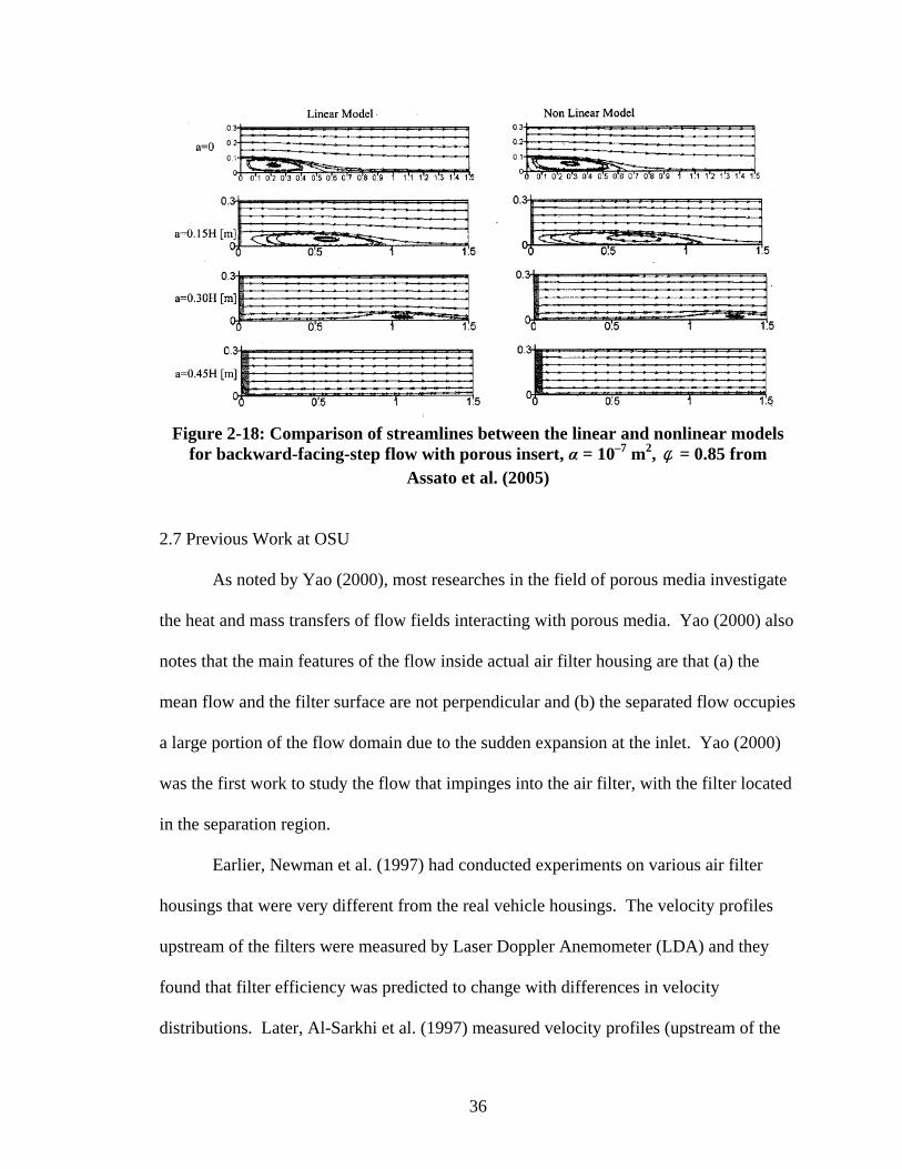
Assato et al. (2005) applied various linear and non-linear k-ε models on flow over
a backward facing step with a porous medium. They found that non-linear models were
better in the prediction of reattachment length even though both types of models under-
predict the experimental value of reattachment length. The effect of thickness of porous
media was found to be more pronounced on the flow than porosity and permeability.
They found that an increase in porous media thickness caused the recirculation to
disappear. See Figures 2-16, 2-17 and 2-18.
35
Figure 2-16: Comparison of streamlines between the linear and nonlinear models for backward-facing-step flow with porous insert, α = 10–6 m2, φ = 0.65 from
Assato et al. (2005)
Figure 2-17: Comparison of streamlines between the linear and nonlinear models
for backward-facing-step flow with porous insert, α = 10–6 m2, φ = 0.85 from
Assato et al. (2005)
36
Figure 2-18: Comparison of streamlines between the linear and nonlinear models
for backward-facing-step flow with porous insert, α = 10–7 m2, φ = 0.85 from Assato et al. (2005)
2.7 Previous Work at OSU
As noted by Yao (2000), most researches in the field of porous media investigate
the heat and mass transfers of flow fields interacting with porous media. Yao (2000) also
notes that the main features of the flow inside actual air filter housing are that (a) the
mean flow and the filter surface are not perpendicular and (b) the separated flow occupies
a large portion of the flow domain due to the sudden expansion at the inlet. Yao (2000)
was the first work to study the flow that impinges into the air filter, with the filter located
in the separation region.
Earlier, Newman et al. (1997) had conducted experiments on various air filter
housings that were very different from the real vehicle housings. The velocity profiles
upstream of the filters were measured by Laser Doppler Anemometer (LDA) and they
found that filter efficiency was predicted to change with differences in velocity
distributions. Later, Al-Sarkhi et al. (1997) measured velocity profiles (upstream of the
37
filter) in housings that were similar in shape to real air-filter housings. Their
experimental results indicated that the filter performance can be enhanced by a uniform
flow impinging normally into the filter. They also found that the mean velocity
distributions are much flatter for flows with filters, due to the resistance offered by the
filter. Also, over the previous decades, the step flow has been a classic test case for many
experiments and numerical simulations. Hence, a large amount of experimental and
numerical data is available, so that the results of our simulations can be compared to
these values and can be validated.
Yao (2000) conducted detailed analyses of a two-dimensional step flow, with and
without the filter. For the no filter laminar case, the numerical results for the
reattachment length match with the experimental results of Armaly et al. (1983) up to
Reynolds number of 650. He found that the when the porous medium is placed at a
location far downstream from the step, it does not affect the separated flow and the
results are almost similar to the no-filter case. However, the porous medium forces the
flow to redistribute i.e. the velocity in the centre decreases and the velocity near the walls
increases. When the porous medium is placed in a location where the non-porous flow is
separated at one side and not separated at the other, he found that the porous medium
caused the flow to reattach at one side and to separate at the other side. Moreover, when
the medium is placed very close to the step, he noted that the separated flow does not
penetrate into the medium. It always re-attached upstream of the porous medium. But,
the secondary re-circulation region was pushed upstream towards the inlet.
Experiments conducted by Yao (2000) were at higher Reynolds number and not
in the laminar regime. This is because; they encountered non-uniform distribution in the
38
seeding particles during LDA measurements in the low Reynolds number experiments.
Measurements were taken at four Reynolds number between 2000 and 10000. Similar
characteristics of re-attachment point were observed in the turbulent flow regime as well.
The re-attachment point in the turbulent flow was independent of the Reynolds number
and more a function of the expansion ratio. Yao (2000) performed LES at various
Reynolds numbers and found that the LES was under predicting the re-attachment length.
However, the LES results obtained by Yao (2000) were not definitive.
2.8 Conclusions of the Review
The review finds that the only numerical analyses that predict the experimental re-
attachment length with good accuracy are the laminar flow analyses (for Re < 600); the
Direct Numerical Simulations (DNS) and Large Eddy Simulations (LES) to some extent.
Very few numerical studies in the literature include Reynolds number range of 2000 to
10000. Experimentation in porous media has been scarce in literature due to the complex
structure of the solid porous matrix. Hence majority of studies in this field (porous
media) are numerical in nature. Moreover, commercial software FLUENT has been used
very rarely in literature to validate experimental studies. Hence, the present study aims to
study the effect of porous media on the re-circulation region formed by the flow over
backward-step by using FLUENT. Through this study, one can examine the performance
of FLUENT in validating macroscopic experiments on porous media.
39
CHAPTER 3
NUMERICAL APPROACH
3.1 Introduction
Simulation of turbulent flows is an extremely challenging problem that has
perplexed researchers for a good part of this century. Turbulent flows are characterized
by unsteady and non-periodic motion. This results in the fluid properties exhibiting
random 3 – D variations. Moreover, there is strong dependence of flow on initial
conditions. The problem is further complicated by the presence of wide range of scales
that require extremely fine grids (if all the scales are resolved). The most advanced
computational tool available to simulate flows is undoubtedly the Direct Numerical
Simulation (DNS). As discussed in Chapter 2, DNS is limited in its application for only
low Reynolds number flows and simple geometries. Moreover, time and space details
obtained from DNS are not required for the present problem of engineering design of air-
filter housings. Time-averaged quantities are suitable for most engineering design
applications.
Large Eddy Simulation (LES) offers some distinct advantages over DNS. In
LES, the computational domain is divided into two distinct scales: (a) large scales, where
Navier-Stokes equations are directly computed and (b) small scales, which are modeled
(as opposed to DNS). As seen from the literature LES has been proven to work well for
40
moderately high Reynolds numbers. The other alternative for flow simulations is the
Reynolds Averaged Navier Stokes (RANS) approach. Decomposing the velocity in
terms of mean velocity and fluctuating velocity (Equation 3.1) followed by time
averaging of the Exact Navier-Stokes equation results in the RANS equation (Equation
3.2)
iii uuu ′+= (3.1)
( ) ( )
( )jij
i
iji
j
j
j
i
jiji
ji
uux
x
u
x
u
x
u
xx
puu
xu
t
′′−∂∂+
∂∂
−∂∂
+∂∂
∂∂+
∂∂−=
∂∂+
∂∂
ρ
δµρρ
3
2
(3.2)
The last term on the right hand side of Equation 3.2: jiuu ′′− ρ are the Reynolds
stresses that need to be modeled. The different approaches of modeling the Reynolds
stresses and the various turbulence models are discussed in detail in Section 3.3.
FLUENT offers the researcher the option of modeling by applying the various turbulence
models including (a) Spalart – Allmaras (b) Standard k-ε (c) RNG k-ε (d) Realizable k-ε
(e) Standard k-ω and (f) Reynolds Stress model. GAMBIT is the pre-processing
software for FLUENT used for creating and meshing 2-D and 3-D models. GAMBIT
was used in the present study for (a) the creation of geometries of Armaly et al. (1983)
and Yao (2000), (b) grid generation and (c) meshing of the geometries.
41
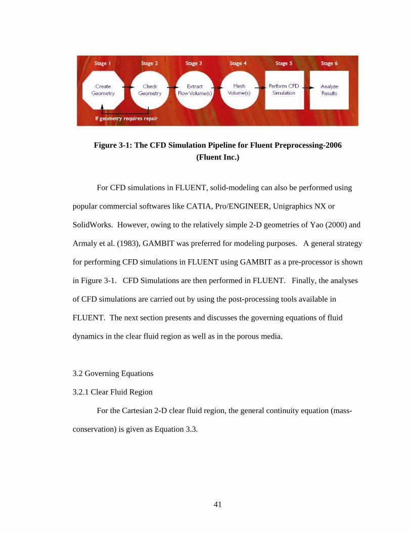
Figure 3-1: The CFD Simulation Pipeline for Fluent Preprocessing-2006
(Fluent Inc.)
For CFD simulations in FLUENT, solid-modeling can also be performed using
popular commercial softwares like CATIA, Pro/ENGINEER, Unigraphics NX or
SolidWorks. However, owing to the relatively simple 2-D geometries of Yao (2000) and
Armaly et al. (1983), GAMBIT was preferred for modeling purposes. A general strategy
for performing CFD simulations in FLUENT using GAMBIT as a pre-processor is shown
in Figure 3-1. CFD Simulations are then performed in FLUENT. Finally, the analyses
of CFD simulations are carried out by using the post-processing tools available in
FLUENT. The next section presents and discusses the governing equations of fluid
dynamics in the clear fluid region as well as in the porous media.
3.2 Governing Equations
3.2.1 Clear Fluid Region
For the Cartesian 2-D clear fluid region, the general continuity equation (mass-
conservation) is given as Equation 3.3.
42
0)( =⋅∇+∂∂
vt
ρρ (3.3)
In the above equation: ρ is the density of air and v is velocity.
( ) Fgpvvvt
++⋅∇+−∇=⋅∇+∂∂ ρτρρ )()( (3.4)
The general form of Newton’s second law (momentum conservation) for the clear
fluid region is given by Equation 3.4. In the above equation, τ is the stress tensor; p is
the pressure drop; gρ is the gravitational force and F is the external body force. For
our problem, the effects of gravity and external body forces are neglected. The stress
tensor is given by Equation 3.5; where in µ is the dynamic viscosity of air.
⋅∇−
∇+∇= Ivvv
T
3
2µτ (3.5)
3.2.2 Porous Region
The fundamentals of flow through porous media are given by Darcy’s equation
(1856). Darcy derived the formula for fluid velocity (v) in terms of the pressure gradient
(∆p) across a porous medium (of length b) and the viscosity of the fluid (µ). The
equation derived by Darcy was purely empirical, given as Equation 3.6.
43
b
Pv
∆−=µα
(3.6)
In the above equation, the constant of proportionality α is called the permeability
of the porous medium. Whitaker (1986) derived Darcy’s equation from the Navier-
Stokes equation by the method of volume averaging (See Equation 3.4). The standard
volume averaged continuity (mass conservation) equation for flow through porous media
is given by Equation 3.7.
0)()( =⋅∇+
∂∂
vt
φρφρ (3.7)
In the above equation, φ is the porosity of the filter. Porosity for any medium is
defined as ratio of the volume of the fluid to the total volume. Equation 3.8 gives the
volume averaged momentum equation for flow through porous media.
vvCvα
µ)τ(p)vvρ(tv)(
221 ρφφφφρ +−⋅∇+∇−=⋅∇+
∂∂
(3.8)
The above Equations 3.7 and 3.8 assume isotropic porosity and are valid only for
single phase flow. The terms vα
µ− and vvC22
1 ρ represent the viscous and inertial
forces due to pore walls on the fluid.
44
3.2.3 Boundary Condition at the Interface of Clear Fluid and Porous Media
FLUENT’s documentation does not elucidate on how the software treats the
boundary condition between the clear fluid and the porous media. The literature talks in
detail regarding various jump conditions namely: stress jump, mass jump, and pressure
jump boundary conditions. However, most of the applications considered were for the
tangential flows rather than normal flows. Kuznetsov (1996) showed that accounting for
a jump in shear-stress at the interface between clear fluid region and the porous media
essentially influences the velocity profiles. Kuznetsov (1996) used the stress-jump
boundary conditions suggested by Ochoa-Tapia and Whitaker (1995).
3.3 Turbulence Models in FLUENT
The following turbulence models are available in FLUENT: the one-equation
Spalart-Allmaras model, various versions of two-equation models and multi-equation
Reynolds Stress model. All the models except the Reynolds Stress Models are based on
the Boussinesq approach. The Boussinesq approach assumes that the turbulent eddy
viscosity is an isotropic quantity which is not precisely true for the majority of the
practical cases. Brief discussions on the various models are presented in this section.
They are Spalart-Allmaras model (SA), k-ε models [Standard k-ε model (SKE); Re-
normalization group k-ε model (RNG); and Realizable k-ε model (RKE)], k-ω models
[Standard k-ω model (SKW) and Shear Stress Transport k-ω model (SST)] and the
Reynolds Stress Model (RSM).
45
3.3.1 Spalart – Allmaras (SA)
The Spalart-Allmaras model is a one equation model based on the Boussinesq
approach. It was developed specifically for aerospace applications that involve wall-
bounded flows. It has been observed that the model performs well for boundary layer
flows with adverse pressure gradients. FLUENT’s User Manual notes that the SA model
is relatively new and has not been validated for all types of engineering flows. To obtain
closure, an additional transport equation for modified turbulent viscosity (ν ) is solved.
3.3.2 Standard k-ε (SKE)
The Standard k-ε model is the most commonly used two-equation turbulent
models and was developed by Jones and Launder (1972). The model solves two
additional differential equations for kinetic energy (k) and dissipation (ε). It is a semi-
empirical model derived from phenomenological analysis and empirical results. The
main advantages of the SKE model are (a) robustness in convergence, (b) cost of
computation and (c) accuracy and applicability for a wide range of complex industrial
flows. The two advanced versions of SKE i.e., RNG and RKE are explained in the
following two sections. These versions have shown to perform better when the flow-field
exhibits vortices, rotation and strong streamline curvature.
3.3.3 Renormalization Group k-ε (RNG)
The RNG model uses a meticulous statistical technique developed by Yakhot and
Orszag (1986). It differs from the SKE model in the following ways:

46
• Additional term in the ε-equation for improved efficiency in case of rapidly
strained flows.
• Includes the effect of swirl on turbulence, thereby performing better for swirling
flows.
• Provides an analytical formula for turbulent Prandtl numbers.
• Accounts for low Reynolds number effects
Thus the RNG model can be applied to a wider range of industrial flows with increased
accuracy.
3.3.4 Realizable k-ε (RKE)
Realizable k-ε model is more accurate than SKE and RNG models for cases
where flow exhibits separation, recirculation, strong pressure gradients etc. FLUENT
user manual defines the term ‘realizable’ as a “model that satisfies some mathematical
constraints on the Reynolds stresses that are consistent with the physics of turbulent
flows”. It differs from SKE in the following manner:
• New formulation of turbulent viscosity (tµ ).
• New transport equation for dissipation (ε), derived from the transport equation for
mean-square vorticity fluctuation.
3.3.5 Standard k-ω (SKW)
The Standard k-ω model is a two-equation turbulence model by Wilcox (1988).
Here, the author refers to ω (specific dissipation rate) as the ratio of ε to k i.e. rate of
dissipation per unit kinetic energy. The SKW model can be applied to both wall-
47
bounded flows and shear flows. The model also incorporates specific changes that
include low Reynolds number effects.
3.3.6 Shear Stress Transport k-ω (SST)
The SST k-ω model was developed by Menter (1994). In this model, the SKW
model is applied in the near wall region whereas the SKE model is incorporated in the
free-stream region of the flow. This is done by converting the SKE model to a SKW
model in the near wall region. A blending function is multiplied to both the models
which are then added together. The function has a value of ‘1’ near the wall thereby
activating SKW model and a value of ‘0’ far away from the wall which triggers the SKE
model. These attributes make the SST model more accurate and reliable than the SKW
model.
3.3.7 Reynolds Stress Model (RSM)
The Reynolds Stress models are the most comprehensive turbulence model option
available in FLUENT. To obtain the closure of RANS equations, transport equation for
Reynolds stresses (from the stress tensor; Equation 3.5) along with dissipation are solved.
Hence, the assumption of isotropic eddy viscosity is not utilized in the RSM models. The
RSM models have the capability to predict complex flow with greater accuracy.
However, FLUENT user manual notes that there may be cases where the simpler
turbulence models might capture the physics of the problem better than the RSM model.
48
3.4 Grid Generation in GAMBIT
Vertices were created by entering their co-ordinates. The units are not important
while creating the grid in GAMBIT, but the simulation in FLUENT always requires the
input parameters to be in S.I. units. For 2-D geometries the z – coordinate is assigned a
default value of zero. Moreover, sufficient distances of 28 h were created downstream of
the step to allow the flow to approach the fully developed condition. Edges were then
created using correct pairs of vertices, followed by faces which were similarly
constructed by grouping together appropriate edges.
The geometry was then checked for corrections and any errors in solid modeling
were edited at this stage. ‘Extracting Flow Volumes or faces (2-D case)’ basically refers
to the exercise of defining the flow path through or around the different solid objects.
The volumes or faces (2-D case) are then meshed in GAMBIT. The number of faces in
any geometry is often the choice of modeler. However, it was observed that finer grids
were better suited to geometries with more faces than those with a single face. Once the
geometry is created, 1–D meshes are created by meshing the edges and finally, 2–D
meshes are then generated by further meshing of the faces.
Both Structured and Unstructured meshes are available in GAMBIT. In the
present study, structured meshing was employed. Boundary conditions types for inlet,
outlet and channel walls were specified and the mesh-file is saved in a binary format for
FLUENT to recognize. Figure 3-2 shows the different edges where boundary conditions
are applied in GAMBIT.
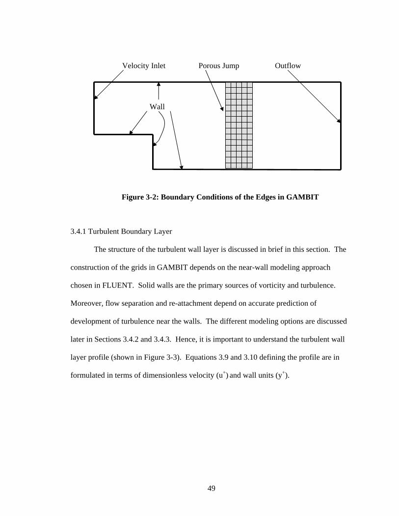
49
Velocity Inlet
Wall
Outflow Porous Jump
3.4.1 Turbulent Boundary Layer
The structure of the turbulent wall layer is discussed in brief in this section. The
construction of the grids in GAMBIT depends on the near-wall modeling approach
chosen in FLUENT. Solid walls are the primary sources of vorticity and turbulence.
Moreover, flow separation and re-attachment depend on accurate prediction of
development of turbulence near the walls. The different modeling options are discussed
later in Sections 3.4.2 and 3.4.3. Hence, it is important to understand the turbulent wall
layer profile (shown in Figure 3-3). Equations 3.9 and 3.10 defining the profile are in
formulated in terms of dimensionless velocity (u+) and wall units (y+).
Figure 3-2: Boundary Conditions of the Edges in GAMBIT
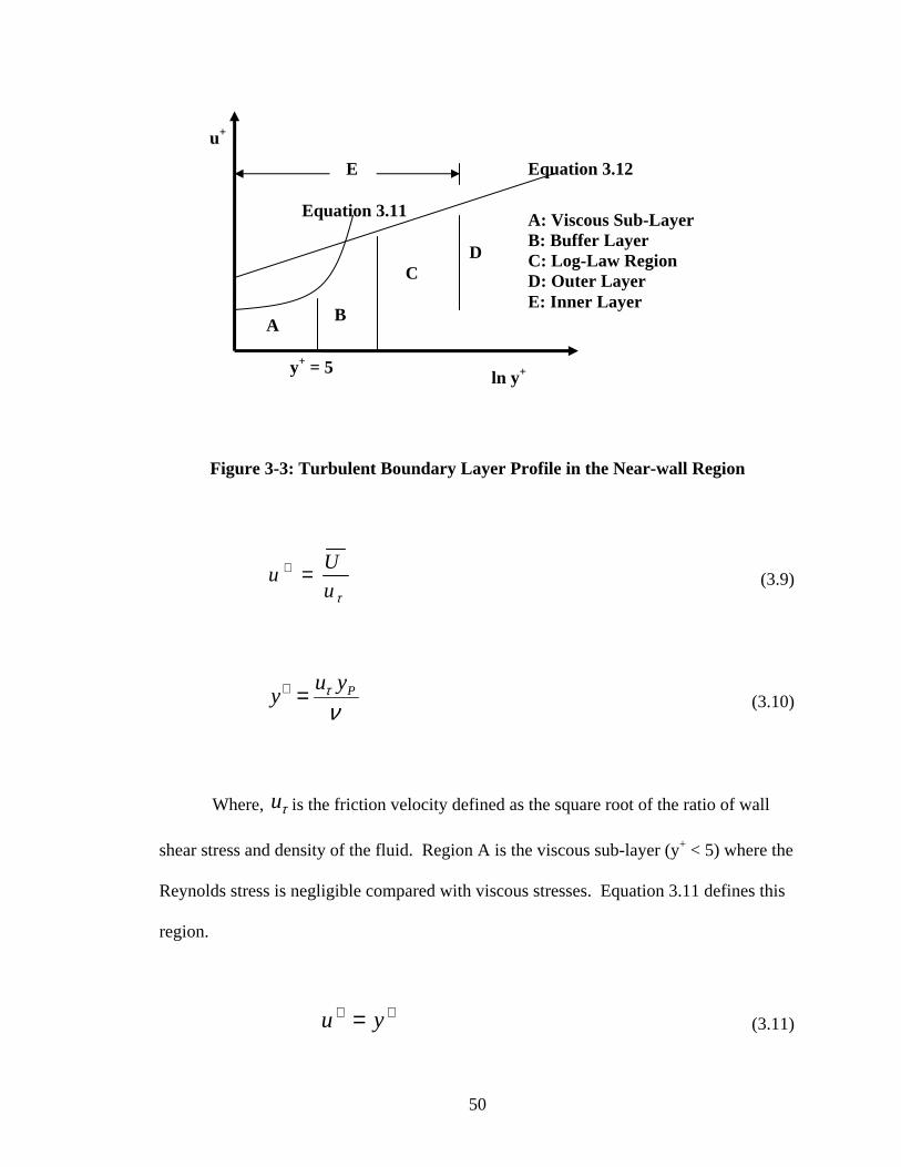
50
Figure 3-3: Turbulent Boundary Layer Profile in the Near-wall Region
τu
Uu =+
(3.9)
ντ Pyu
y =+ (3.10)
Where, τu is the friction velocity defined as the square root of the ratio of wall
shear stress and density of the fluid. Region A is the viscous sub-layer (y+ < 5) where the
Reynolds stress is negligible compared with viscous stresses. Equation 3.11 defines this
region.
++ = yu (3.11)
A: Viscous Sub-Layer B: Buffer Layer C: Log-Law Region D: Outer Layer E: Inner Layer
u+
ln y+
A B
C D
E Equation 3.12
Equation 3.11
y+ = 5
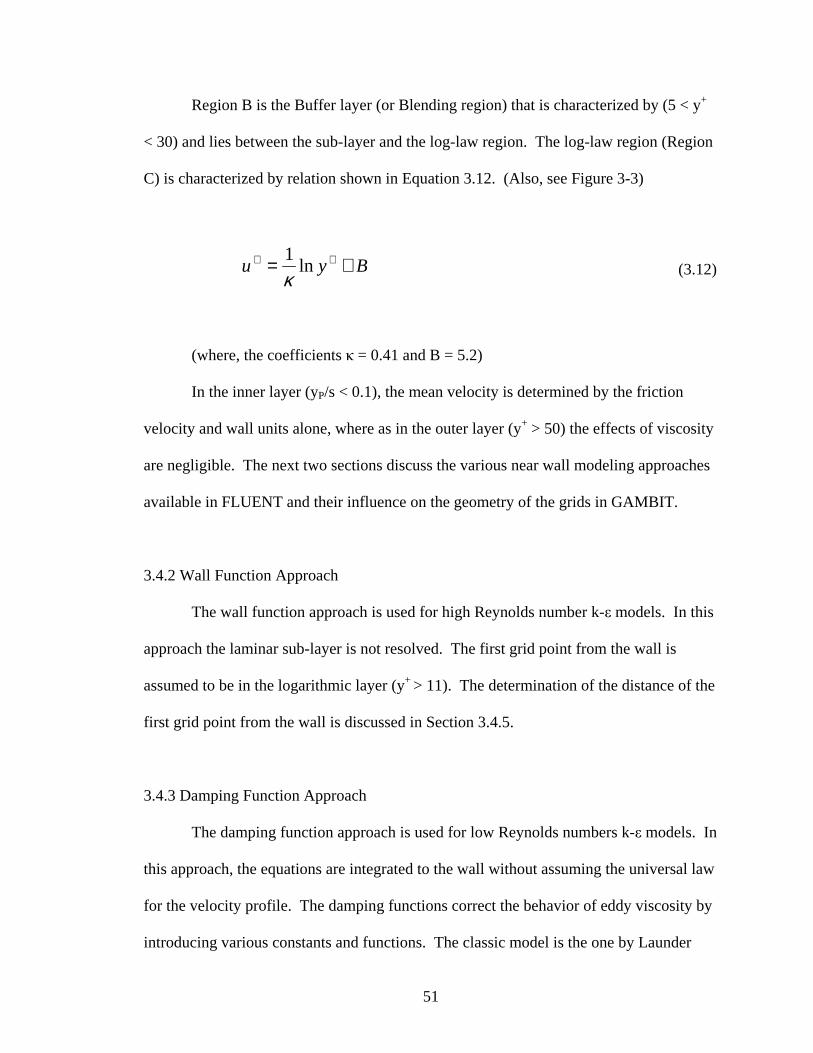
51
Region B is the Buffer layer (or Blending region) that is characterized by (5 < y+
< 30) and lies between the sub-layer and the log-law region. The log-law region (Region
C) is characterized by relation shown in Equation 3.12. (Also, see Figure 3-3)
Byu += ++ ln1
κ (3.12)
(where, the coefficients κ = 0.41 and B = 5.2)
In the inner layer (yP/s < 0.1), the mean velocity is determined by the friction
velocity and wall units alone, where as in the outer layer (y+ > 50) the effects of viscosity
are negligible. The next two sections discuss the various near wall modeling approaches
available in FLUENT and their influence on the geometry of the grids in GAMBIT.
3.4.2 Wall Function Approach
The wall function approach is used for high Reynolds number k-ε models. In this
approach the laminar sub-layer is not resolved. The first grid point from the wall is
assumed to be in the logarithmic layer (y+ > 11). The determination of the distance of the
first grid point from the wall is discussed in Section 3.4.5.
3.4.3 Damping Function Approach
The damping function approach is used for low Reynolds numbers k-ε models. In
this approach, the equations are integrated to the wall without assuming the universal law
for the velocity profile. The damping functions correct the behavior of eddy viscosity by
introducing various constants and functions. The classic model is the one by Launder
52
and Sharma (1972). It has been observed from the literature that the model predicts
incorrect results (when compared to DNS and experimental results) for k and ε,
especially near the solid walls.
3.4.4 Two Layer Model Approach
In this approach the grid is separated into two different regions: (a) near wall
region, where the effects of viscosity are taken into account and typically the k-ω model
is applied (b) a fully turbulent outer region where the standard k-ε is applied. A region of
y+ ≈ 30 is chosen by FLUENT to distinguish the two layers.
3.4.5 Determination of Distance of First Grid Point from the Wall
The distance (yP) can be obtained from Equation 3.10 which is re-stated below as
Equation 3.13.
τρµ
u
yyP
+
= (3.13)
Hence, in order to determine y, one needs to obtain the value of τu . This is done
by using the definition of Reynolds number based on friction velocity, as shown in
Equation 3.14. Moreover, τRe can be read directly from Figure 3-4, which shows
τRe as a function of Re (based on channel height).
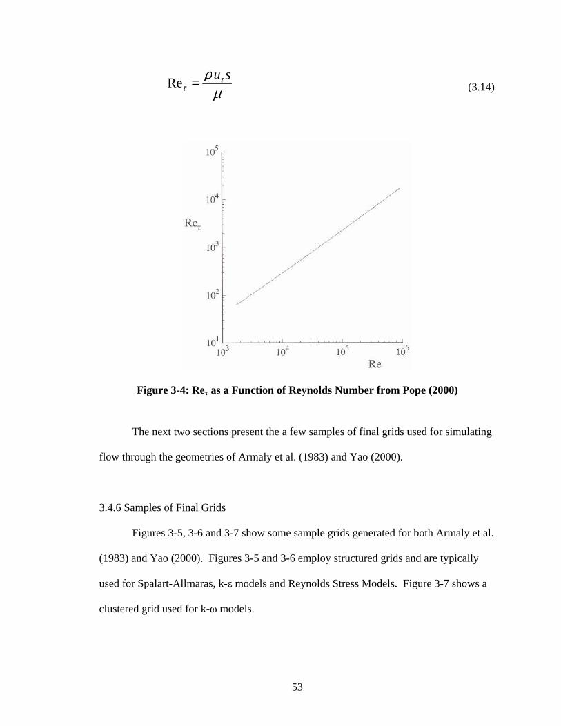
53
µρ τ
τsu=Re (3.14)
Figure 3-4: Reτ as a Function of Reynolds Number from Pope (2000)
The next two sections present the a few samples of final grids used for simulating
flow through the geometries of Armaly et al. (1983) and Yao (2000).
3.4.6 Samples of Final Grids
Figures 3-5, 3-6 and 3-7 show some sample grids generated for both Armaly et al.
(1983) and Yao (2000). Figures 3-5 and 3-6 employ structured grids and are typically
used for Spalart-Allmaras, k-ε models and Reynolds Stress Models. Figure 3-7 shows a
clustered grid used for k-ω models.
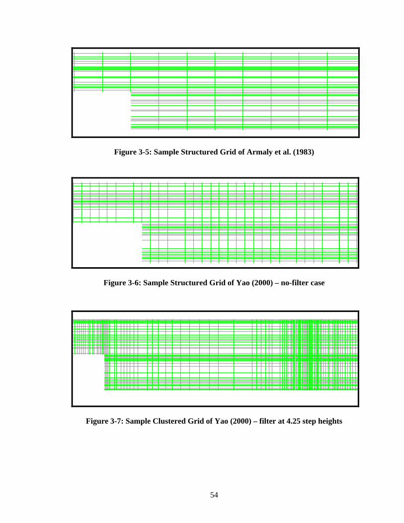
54
Figure 3-5: Sample Structured Grid of Armaly et al. (1983)
Figure 3-6: Sample Structured Grid of Yao (2000) – no-filter case
Figure 3-7: Sample Clustered Grid of Yao (2000) – filter at 4.25 step heights

55
3.5 Simulation in FLUENT
The user interface of FLUENT is written in a language called ‘Scheme’. Scheme
is a dialect of the software language LISP. FLUENT allows the user to write menu
macros and functions, thus enabling the advanced user to customize the interface. The
menu driven interface of FLUENT is run using a UNIX (Sun Solaris) platform. The
following modeling steps are performed for running simulations in FLUENT:
1. Reading the grid file (in .msh format): File → Read → Case…
The grid that is already constructed in GAMBIT is saved as a (.msh) file.
This file is imported and read into FLUENT.
2. Checking the grid: Grid→ Check…
This is done to ensure that there are no ‘negative cell volumes’ in the grid.
Negative cell volumes are indications of improper connectivity in the grid that
must be avoided.
3. Specifying solver properties: Define → Models →Solver…
Options are available in FLUENT for choosing (a) Segregated or (b)
Coupled solvers. In segregated solvers the continuity and momentum equations
are solved separately while in coupled solvers the equations are solved
simultaneously. Figure 4 shows default options given by FLUENT.
4. Selecting the physical models: Define → Models → Viscous…
Depending on whether the flow is laminar or turbulent, the physical models
are chosen. The default values of constants provided by FLUENT can also
changed by the user.
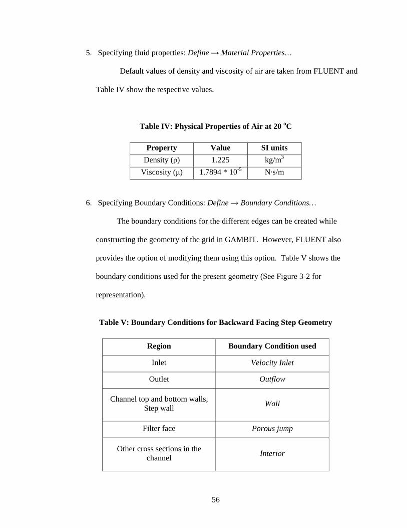
56
5. Specifying fluid properties: Define → Material Properties…
Default values of density and viscosity of air are taken from FLUENT and
Table IV show the respective values.
Table IV: Physical Properties of Air at 20 oC
Property Value SI units
Density (ρ) 1.225 kg/m3
Viscosity (µ) 1.7894 * 10-5 N·s/m
6. Specifying Boundary Conditions: Define → Boundary Conditions…
The boundary conditions for the different edges can be created while
constructing the geometry of the grid in GAMBIT. However, FLUENT also
provides the option of modifying them using this option. Table V shows the
boundary conditions used for the present geometry (See Figure 3-2 for
representation).
Table V: Boundary Conditions for Backward Facing Step Geometry
Region Boundary Condition used
Inlet Velocity Inlet
Outlet Outflow
Channel top and bottom walls, Step wall
Wall
Filter face Porous jump
Other cross sections in the channel
Interior
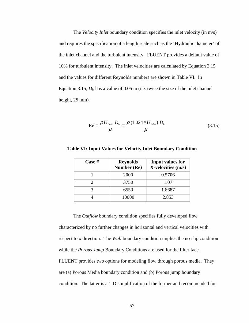
57
The Velocity Inlet boundary condition specifies the inlet velocity (in m/s)
and requires the specification of a length scale such as the ‘Hydraulic diameter’ of
the inlet channel and the turbulent intensity. FLUENT provides a default value of
10% for turbulent intensity. The inlet velocities are calculated by Equation 3.15
and the values for different Reynolds numbers are shown in Table VI. In
Equation 3.15, Dh has a value of 0.05 m (i.e. twice the size of the inlet channel
height, 25 mm).
µρ
µρ hinlethbulk DUDU )024.1(
Re×== (3.15)
Table VI: Input Values for Velocity Inlet Boundary Condition
Case # Reynolds
Number (Re) Input values for X-velocities (m/s)
1 2000 0.5706
2 3750 1.07
3 6550 1.8687
4 10000 2.853
The Outflow boundary condition specifies fully developed flow
characterized by no further changes in horizontal and vertical velocities with
respect to x direction. The Wall boundary condition implies the no-slip condition
while the Porous Jump Boundary Conditions are used for the filter face.
FLUENT provides two options for modeling flow through porous media. They
are (a) Porous Media boundary condition and (b) Porous jump boundary
condition. The latter is a 1-D simplification of the former and recommended for
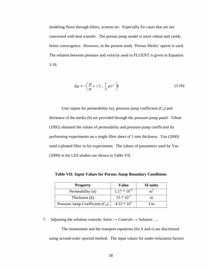
58
modeling flows through filters, screens etc. Especially for cases that are not
concerned with heat transfer. The porous jump model is more robust and yields
better convergence. However, in the present study ‘Porous Media’ option is used.
The relation between pressure and velocity used in FLUENT is given in Equation
3.16.
bvCvp
+−=∆ 22 2
1 ραµ (3.16)
User inputs for permeability (α), pressure jump coefficient (C2) and
thickness of the media (b) are provided through the pressure-jump panel. Tebutt
(1995) obtained the values of permeability and pressure-jump coefficient by
performing experiments on a single filter sheet of 1 mm thickness. Yao (2000)
used a pleated filter in his experiments. The values of parameters used by Yao
(2000) in his LES studies are shown in Table VII.
Table VII: Input Values for Porous Jump Boundary Conditions
Property Value SI units
Permeability (α) 1.17 * 10-9 m2
Thickness (b) 15 * 10-3 m
Pressure Jump Coefficient (C2) 4.53 * 103 1/m
7. Adjusting the solution controls: Solve → Controls → Solution …
The momentum and the transport equations (for k and ε) are discretized
using second-order upwind method. The input values for under-relaxation factors
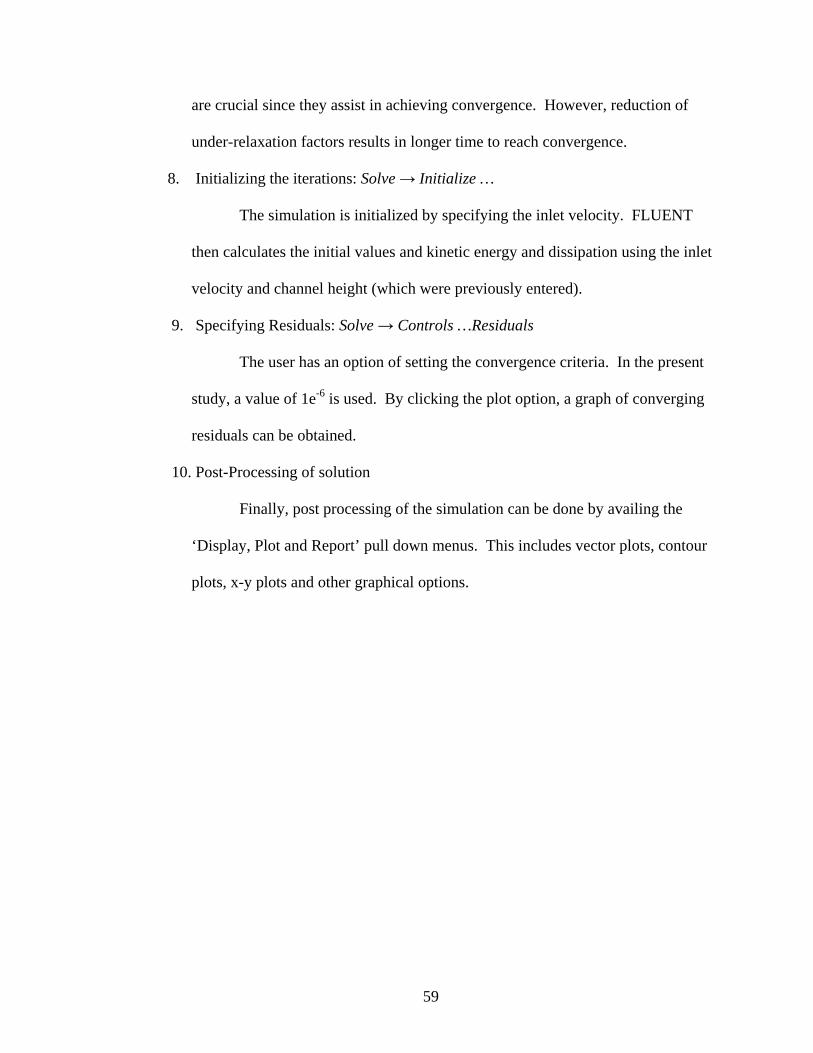
59
are crucial since they assist in achieving convergence. However, reduction of
under-relaxation factors results in longer time to reach convergence.
8. Initializing the iterations: Solve → Initialize …
The simulation is initialized by specifying the inlet velocity. FLUENT
then calculates the initial values and kinetic energy and dissipation using the inlet
velocity and channel height (which were previously entered).
9. Specifying Residuals: Solve → Controls …Residuals
The user has an option of setting the convergence criteria. In the present
study, a value of 1e-6 is used. By clicking the plot option, a graph of converging
residuals can be obtained.
10. Post-Processing of solution
Finally, post processing of the simulation can be done by availing the
‘Display, Plot and Report’ pull down menus. This includes vector plots, contour
plots, x-y plots and other graphical options.
60
CHAPTER 4
RESULTS AND DISCUSSION
4.1 Grid Independence Studies
It is extremely important in Computational Fluid Dynamics for the simulation to
represent correctly the conceptual model. Moreover, the simulation should resemble
real- life flows to the greatest accuracy possible. Numerical Simulations have various
advantages over experiments. The primary one being that parameters can easily be
changed and quick results are possible at lower costs. The details of the numerical
methods and FLUENT software employed can be found from Chapter 3. In this section,
grid independence studies are carried out for the geometries of Armaly et al. (1983) and
Yao (2000). Moreover, the turbulent model that most closely resembles the real-world
flow will be chosen for simulating two-dimensional step flows with and without the filter.
Re-attachment length is used as a criterion for comparing different turbulent models and
thus ensuring that the simulated flow closely resembles true experimental results. The
phenomena of flow separation and re-attachment length are strongly dependent on the
correct prediction of the development of turbulence near the walls. Also, excessive
numerical diffusion caused by grid-density may incorrectly enhance the viscous effects
leading to inaccurate simulations. This exercise enables us to observe the sensitivities of
61
the dependent variable (in our case: Re-attachment length) on multiple refined spatial
grids (AIAA Editorial Policy Statement).
For an accurate CFD simulation, quantifying uncertainty and error is very
essential. Typically, uncertainties refer to lack of knowledge regarding modeling
parameters while errors refer to a deficiency that has not been caused by lack of
knowledge. In our present simulations, the assumption of the log-law in the near wall
region in the re-circulation zone can be considered as an uncertainty. The main sources
of error (AIAA G-077) that need to be paid attention to are insufficient spatial or
temporal discretization convergence, lack of iterative convergence and other
programming errors. It is generally recommended that discretization employed be at
least second-order accurate. Moreover, AIAA Editorial policy states that the solution
also be compared to a highly accurate numerical solution. For iterative convergence, the
value of residual error (magnitude of difference between both sides of the difference
equations) should be set to a very low value [Roache (2002)]. In the present study, it is
set to 1e-6. The inlet velocities for both geometries are calculated from the Reynolds
numbers for which the experiments are planned to be validated. For the outlet, fully
developed conditions are confirmed by observation of downstream velocity profiles. The
next two sections present the results of grid independence studies on the geometries of
Armaly et al. (1983) and Yao et al. (2000).
4.1.1 Grid Independence: Armaly et al. (1983)
Grid Independence studies were conducted at Re = 7000 for the backward-facing
step geometry of Armaly et al. (1983). The experimental re-attachment length from
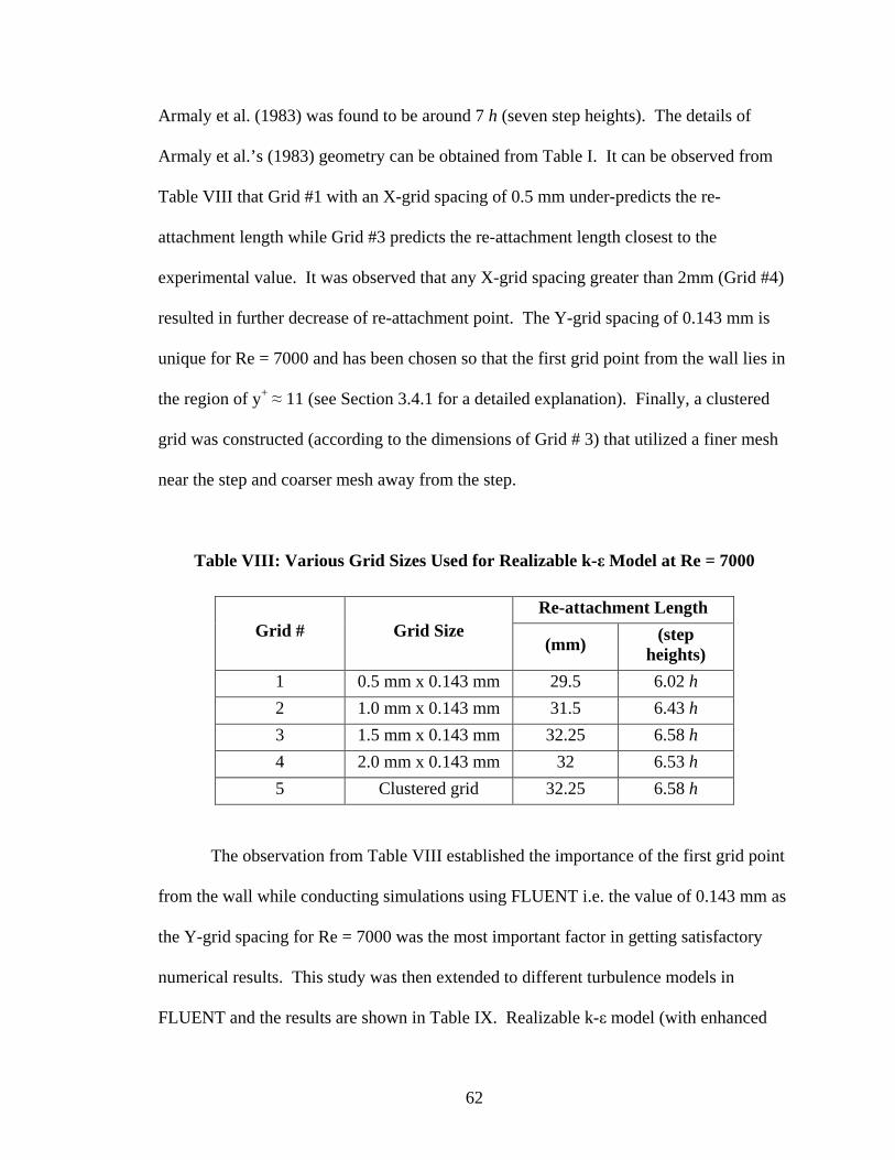
62
Armaly et al. (1983) was found to be around 7 h (seven step heights). The details of
Armaly et al.’s (1983) geometry can be obtained from Table I. It can be observed from
Table VIII that Grid #1 with an X-grid spacing of 0.5 mm under-predicts the re-
attachment length while Grid #3 predicts the re-attachment length closest to the
experimental value. It was observed that any X-grid spacing greater than 2mm (Grid #4)
resulted in further decrease of re-attachment point. The Y-grid spacing of 0.143 mm is
unique for Re = 7000 and has been chosen so that the first grid point from the wall lies in
the region of y+ ≈ 11 (see Section 3.4.1 for a detailed explanation). Finally, a clustered
grid was constructed (according to the dimensions of Grid # 3) that utilized a finer mesh
near the step and coarser mesh away from the step.
Table VIII: Various Grid Sizes Used for Realizable k-ε Model at Re = 7000
Re-attachment Length
Grid # Grid Size (mm) (step
heights)
1 0.5 mm x 0.143 mm 29.5 6.02 h
2 1.0 mm x 0.143 mm 31.5 6.43 h
3 1.5 mm x 0.143 mm 32.25 6.58 h
4 2.0 mm x 0.143 mm 32 6.53 h
5 Clustered grid 32.25 6.58 h
The observation from Table VIII established the importance of the first grid point
from the wall while conducting simulations using FLUENT i.e. the value of 0.143 mm as
the Y-grid spacing for Re = 7000 was the most important factor in getting satisfactory
numerical results. This study was then extended to different turbulence models in
FLUENT and the results are shown in Table IX. Realizable k-ε model (with enhanced
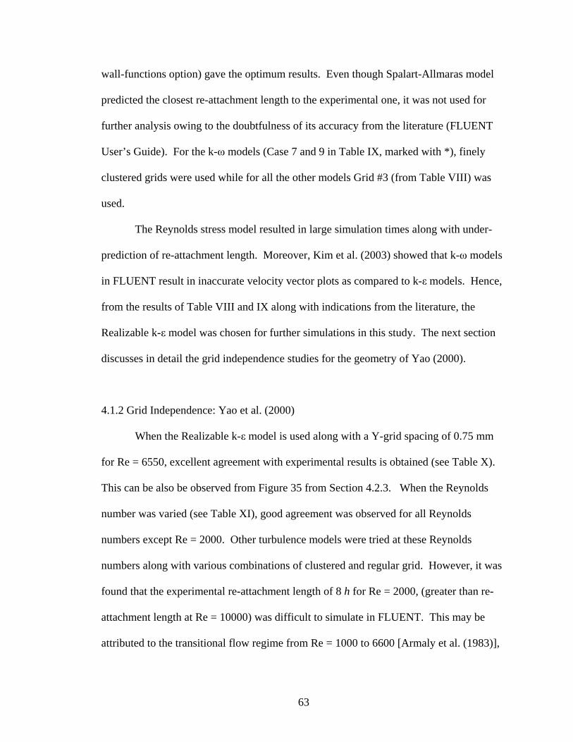
63
wall-functions option) gave the optimum results. Even though Spalart-Allmaras model
predicted the closest re-attachment length to the experimental one, it was not used for
further analysis owing to the doubtfulness of its accuracy from the literature (FLUENT
User’s Guide). For the k-ω models (Case 7 and 9 in Table IX, marked with *), finely
clustered grids were used while for all the other models Grid #3 (from Table VIII) was
used.
The Reynolds stress model resulted in large simulation times along with under-
prediction of re-attachment length. Moreover, Kim et al. (2003) showed that k-ω models
in FLUENT result in inaccurate velocity vector plots as compared to k-ε models. Hence,
from the results of Table VIII and IX along with indications from the literature, the
Realizable k-ε model was chosen for further simulations in this study. The next section
discusses in detail the grid independence studies for the geometry of Yao (2000).
4.1.2 Grid Independence: Yao et al. (2000)
When the Realizable k-ε model is used along with a Y-grid spacing of 0.75 mm
for Re = 6550, excellent agreement with experimental results is obtained (see Table X).
This can be also be observed from Figure 35 from Section 4.2.3. When the Reynolds
number was varied (see Table XI), good agreement was observed for all Reynolds
numbers except Re = 2000. Other turbulence models were tried at these Reynolds
numbers along with various combinations of clustered and regular grid. However, it was
found that the experimental re-attachment length of 8 h for Re = 2000, (greater than re-
attachment length at Re = 10000) was difficult to simulate in FLUENT. This may be
attributed to the transitional flow regime from Re = 1000 to 6600 [Armaly et al. (1983)],
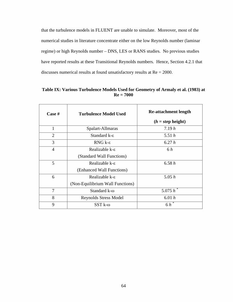
64
that the turbulence models in FLUENT are unable to simulate. Moreover, most of the
numerical studies in literature concentrate either on the low Reynolds number (laminar
regime) or high Reynolds number – DNS, LES or RANS studies. No previous studies
have reported results at these Transitional Reynolds numbers. Hence, Section 4.2.1 that
discusses numerical results at found unsatisfactory results at Re = 2000.
Table IX: Various Turbulence Models Used for Geometry of Armaly et al. (1983) at Re = 7000
Case #
Turbulence Model Used Re-attachment length
(h = step height)
1 Spalart-Allmaras 7.19 h
2 Standard k-ε 5.51 h
3 RNG k-ε 6.27 h
4 Realizable k-ε
(Standard Wall Functions)
6 h
5 Realizable k-ε
(Enhanced Wall Functions)
6.58 h
6 Realizable k-ε
(Non-Equilibrium Wall Functions)
5.05 h
7 Standard k-ω 5.075 h *
8 Reynolds Stress Model 6.01 h
9 SST k-ω 6 h *
65
Table X: Various Grid Sizes Used for Geometry of Yao (2000); Realizable k-ε Model at Re = 6550
Re-attachment Length
Grid # Grid Size (mm) (step heights)
1 0.5 mm x 0.75 mm 29.5 6.13 h
2 1.5 mm x 0.75 mm 31.5 6.42 h
3 2.5 mm x 0.75 mm 32.25 6.32 h
4 3.5 mm x 0.75 mm 32 6.37 h
5 Clustered 32.25 6.32 h
Also, as discussed in Section 3.6, the porous jump boundary conditions used in
FLUENT at the interface between the clear-fluid region and the porous media is not
documented well in the FLUENT User’s guide. Hence, important details on how
FLUENT treats this boundary condition are missing in this study. This may be one of the
important factors affecting numerical results found in the present study.
Table XI: Re-attachment Lengths at Different Reynolds Numbers Using
Realizable k-ε model
Re-attachment Length Reynolds
Number Grid Size Experimental FLUENT
2000 3.5 mm x 2 mm 8 4.9 h
3750 3.5 mm x 1.15 mm 6 6.23 h
6550 3.5 mm x 0.75 mm 6.5 6.37 h
10000 3.5 mm x 0.5 mm 7 6.6 h
4.2 Numerical Results from FLUENT
4.2.1 Re = 2000 and Re = 3750
Separation lines (as seen from Figure 4-1), provide a good indication of the flow
field physics along with the re-attachment point. Each point on the separation line
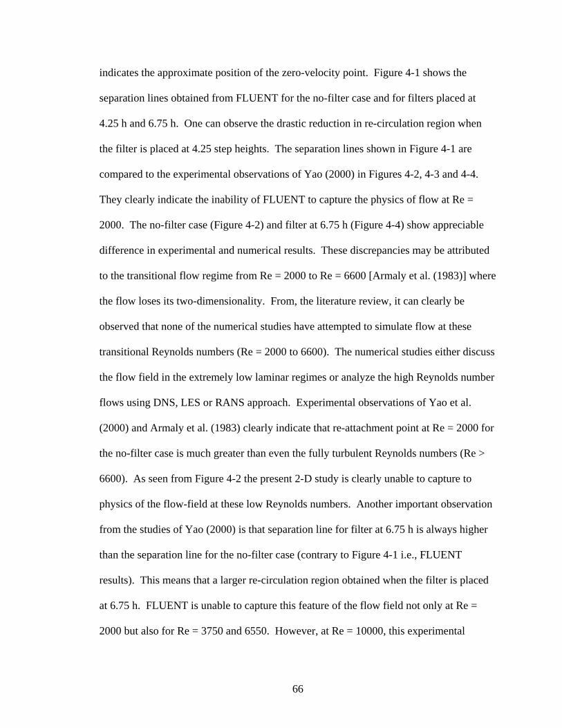
66
indicates the approximate position of the zero-velocity point. Figure 4-1 shows the
separation lines obtained from FLUENT for the no-filter case and for filters placed at
4.25 h and 6.75 h. One can observe the drastic reduction in re-circulation region when
the filter is placed at 4.25 step heights. The separation lines shown in Figure 4-1 are
compared to the experimental observations of Yao (2000) in Figures 4-2, 4-3 and 4-4.
They clearly indicate the inability of FLUENT to capture the physics of flow at Re =
2000. The no-filter case (Figure 4-2) and filter at 6.75 h (Figure 4-4) show appreciable
difference in experimental and numerical results. These discrepancies may be attributed
to the transitional flow regime from Re = 2000 to Re = 6600 [Armaly et al. (1983)] where
the flow loses its two-dimensionality. From, the literature review, it can clearly be
observed that none of the numerical studies have attempted to simulate flow at these
transitional Reynolds numbers (Re = 2000 to 6600). The numerical studies either discuss
the flow field in the extremely low laminar regimes or analyze the high Reynolds number
flows using DNS, LES or RANS approach. Experimental observations of Yao et al.
(2000) and Armaly et al. (1983) clearly indicate that re-attachment point at Re = 2000 for
the no-filter case is much greater than even the fully turbulent Reynolds numbers (Re >
6600). As seen from Figure 4-2 the present 2-D study is clearly unable to capture to
physics of the flow-field at these low Reynolds numbers. Another important observation
from the studies of Yao (2000) is that separation line for filter at 6.75 h is always higher
than the separation line for the no-filter case (contrary to Figure 4-1 i.e., FLUENT
results). This means that a larger re-circulation region obtained when the filter is placed
at 6.75 h. FLUENT is unable to capture this feature of the flow field not only at Re =
2000 but also for Re = 3750 and 6550. However, at Re = 10000, this experimental
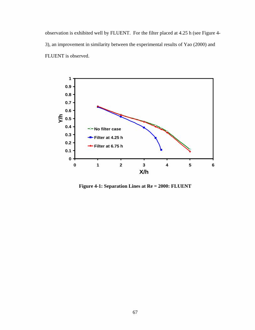
67
observation is exhibited well by FLUENT. For the filter placed at 4.25 h (see Figure 4-
3), an improvement in similarity between the experimental results of Yao (2000) and
FLUENT is observed.
0
0.1
0.2
0.3
0.4
0.5
0.6
0.7
0.8
0.9
1
0 1 2 3 4 5 6
X/h
Y/h
No filter case
Filter at 4.25 h
Filter at 6.75 h
Figure 4-1: Separation Lines at Re = 2000: FLUENT
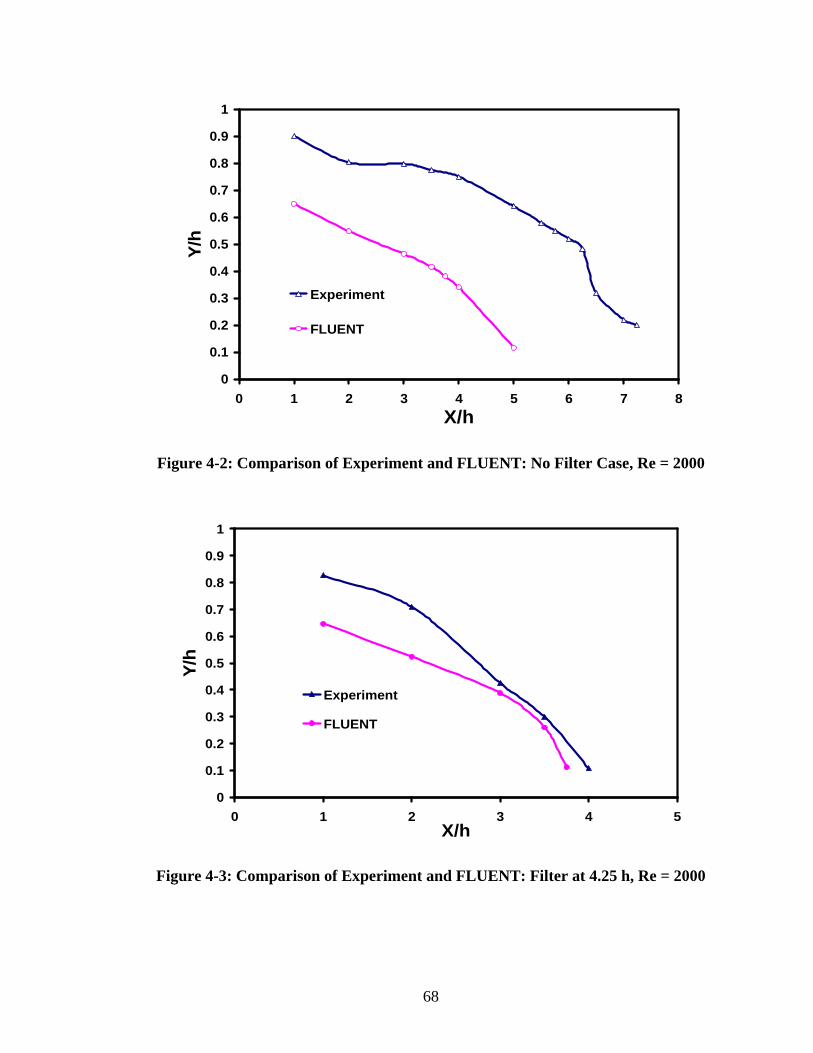
68
0
0.1
0.2
0.3
0.4
0.5
0.6
0.7
0.8
0.9
1
0 1 2 3 4 5 6 7 8
X/h
Y/h
Experiment
FLUENT
Figure 4-2: Comparison of Experiment and FLUENT: No Filter Case, Re = 2000
0
0.1
0.2
0.3
0.4
0.5
0.6
0.7
0.8
0.9
1
0 1 2 3 4 5X/h
Y/h
Experiment
FLUENT
Figure 4-3: Comparison of Experiment and FLUENT: Filter at 4.25 h, Re = 2000
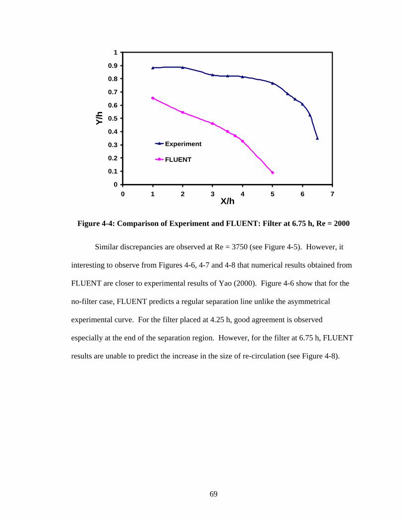
69
0
0.1
0.2
0.3
0.4
0.5
0.6
0.7
0.8
0.9
1
0 1 2 3 4 5 6 7X/h
Y/h
Experiment
FLUENT
Figure 4-4: Comparison of Experiment and FLUENT: Filter at 6.75 h, Re = 2000
Similar discrepancies are observed at Re = 3750 (see Figure 4-5). However, it
interesting to observe from Figures 4-6, 4-7 and 4-8 that numerical results obtained from
FLUENT are closer to experimental results of Yao (2000). Figure 4-6 show that for the
no-filter case, FLUENT predicts a regular separation line unlike the asymmetrical
experimental curve. For the filter placed at 4.25 h, good agreement is observed
especially at the end of the separation region. However, for the filter at 6.75 h, FLUENT
results are unable to predict the increase in the size of re-circulation (see Figure 4-8).
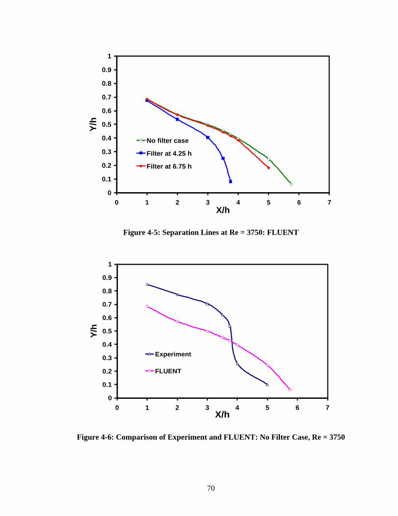
70
0
0.1
0.2
0.3
0.4
0.5
0.6
0.7
0.8
0.9
1
0 1 2 3 4 5 6 7X/h
Y/h
No filter case
Filter at 4.25 h
Filter at 6.75 h
Figure 4-5: Separation Lines at Re = 3750: FLUENT
0
0.1
0.2
0.3
0.4
0.5
0.6
0.7
0.8
0.9
1
0 1 2 3 4 5 6 7X/h
Y/h
Experiment
FLUENT
Figure 4-6: Comparison of Experiment and FLUENT: No Filter Case, Re = 3750
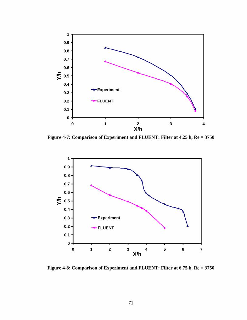
71
0
0.1
0.2
0.3
0.4
0.5
0.6
0.7
0.8
0.9
1
0 1 2 3 4X/h
Y/h
Experiment
FLUENT
Figure 4-7: Comparison of Experiment and FLUENT: Filter at 4.25 h, Re = 3750
0
0.1
0.2
0.3
0.4
0.5
0.6
0.7
0.8
0.9
1
0 1 2 3 4 5 6 7X/h
Y/h
Experiment
FLUENT
Figure 4-8: Comparison of Experiment and FLUENT: Filter at 6.75 h, Re = 3750
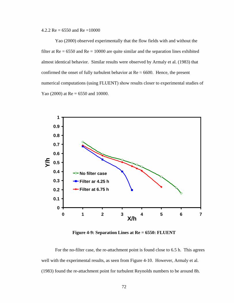
72
4.2.2 Re = 6550 and Re =10000
Yao (2000) observed experimentally that the flow fields with and without the
filter at Re = 6550 and Re = 10000 are quite similar and the separation lines exhibited
almost identical behavior. Similar results were observed by Armaly et al. (1983) that
confirmed the onset of fully turbulent behavior at Re ≈ 6600. Hence, the present
numerical computations (using FLUENT) show results closer to experimental studies of
Yao (2000) at Re = 6550 and 10000.
0
0.1
0.2
0.3
0.4
0.5
0.6
0.7
0.8
0.9
1
0 1 2 3 4 5 6 7X/h
Y/h
No filter case
Filter ar 4.25 h
Filter at 6.75 h
Figure 4-9: Separation Lines at Re = 6550: FLUENT
For the no-filter case, the re-attachment point is found close to 6.5 h. This agrees
well with the experimental results, as seen from Figure 4-10. However, Armaly et al.
(1983) found the re-attachment point for turbulent Reynolds numbers to be around 8h.
73
This difference as noted by Yao (2000) may be due to various factors like difference in
inlet RMS velocity profiles etc. Moreover, in the present studies, no evidence of non-
step side vortex was found at Re = 6550. This observation agrees well with the
experimental results of both Yao (2000) and Armaly et al. (1983). When the filter is
placed at 4.25 step heights (see Figure 4-9), the re-circulation region is greatly reduced.
Figure 4-11 shows that after 2h, the experimental and present results agree to some
extent. The filter when placed at 4.25 h greatly alters the flow field as compared to the
no-filter case. From Figure 4-13, one observes that the filter pushes the maximum
velocity region towards the centre of the channel to present a symmetrical profile, while
the no-filter case exhibits an unsymmetrical velocity distribution. Similar trends are
observed for the velocity profiles from the studies of Yao (2000). For the filter placed at
6.75 step heights, FLUENT shows a smaller re-circulation region as contrary to
experimental analyses. Moreover, a shorter re-attachment length is observed (see Figures
4-11 and 4-12). This shows that in the present numerical studies, filter placed at 6.75 h
still affects the flow field while no such evidence is found experimentally. Figure 4-14
shows the comparison of velocity profiles at 5h. It can be observed that it agrees well
with the trends exhibited by the no-filter case. However, after 5h, the filter case (6.75h)
re-attaches quickly while no-filter case flow (experiment and FLUENT) predicts longer
reattachment length.
The following conclusions can be drawn for FLUENT simulations at Re = 6550.
The no-filter case and filter at 4.25 h (see Figures 4-10 and 4-11) is simulated well by
FLUENT. The case of the filter placed at 6.75 h still exhibits the influence of the filter
on the flow field. These discrepancies may be due to the inability of FLUENT and/or the
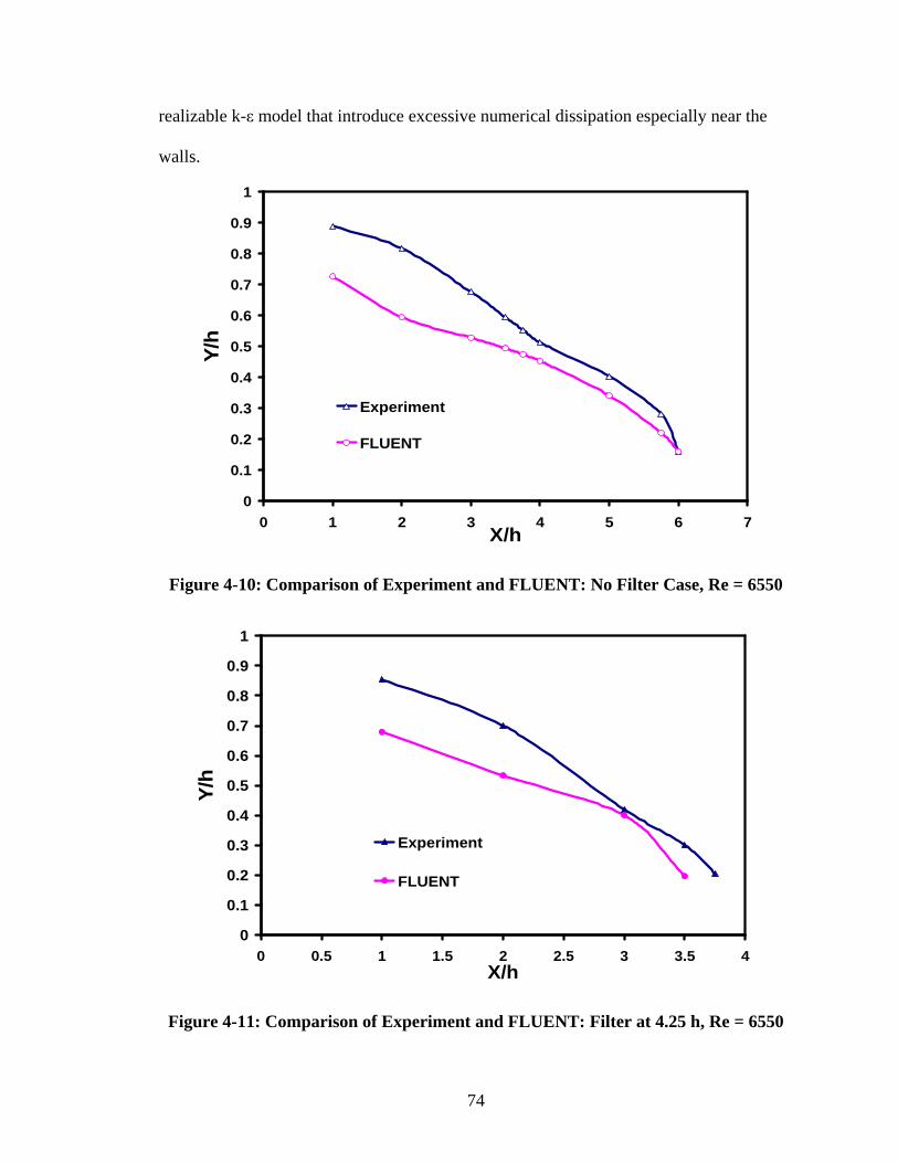
74
realizable k-ε model that introduce excessive numerical dissipation especially near the
walls.
0
0.1
0.2
0.3
0.4
0.5
0.6
0.7
0.8
0.9
1
0 1 2 3 4 5 6 7X/h
Y/h
Experiment
FLUENT
Figure 4-10: Comparison of Experiment and FLUENT: No Filter Case, Re = 6550
0
0.1
0.2
0.3
0.4
0.5
0.6
0.7
0.8
0.9
1
0 0.5 1 1.5 2 2.5 3 3.5 4X/h
Y/h
Experiment
FLUENT
Figure 4-11: Comparison of Experiment and FLUENT: Filter at 4.25 h, Re = 6550
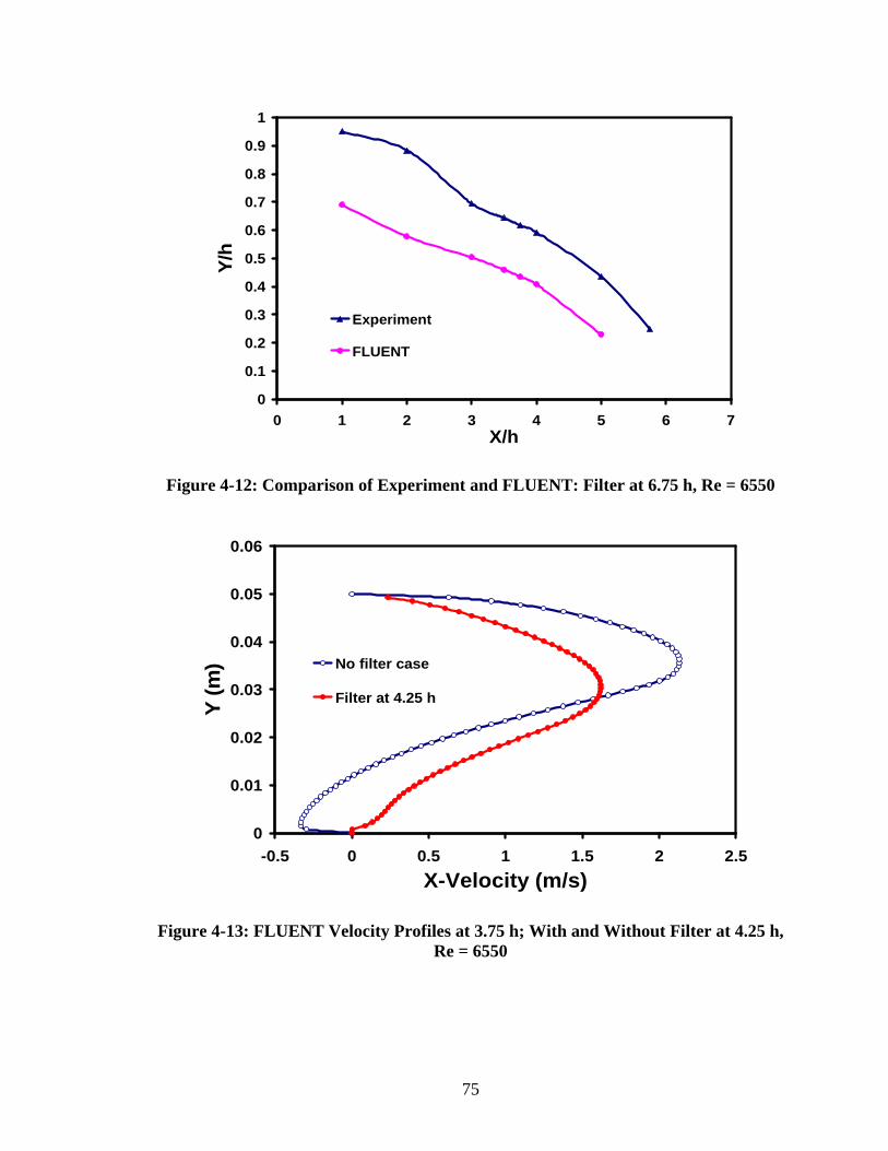
75
0
0.1
0.2
0.3
0.4
0.5
0.6
0.7
0.8
0.9
1
0 1 2 3 4 5 6 7X/h
Y/h
Experiment
FLUENT
Figure 4-12: Comparison of Experiment and FLUENT: Filter at 6.75 h, Re = 6550
0
0.01
0.02
0.03
0.04
0.05
0.06
-0.5 0 0.5 1 1.5 2 2.5
X-Velocity (m/s)
Y (
m) No filter case
Filter at 4.25 h
Figure 4-13: FLUENT Velocity Profiles at 3.75 h; With and Without Filter at 4.25 h, Re = 6550
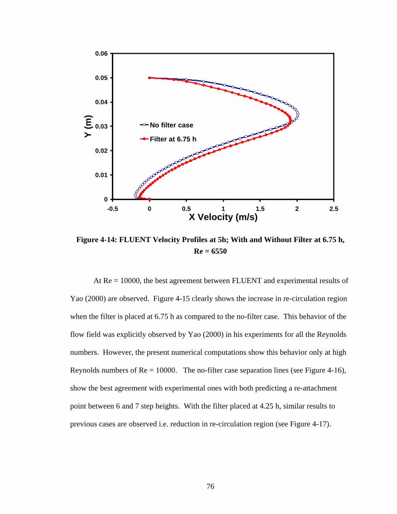
76
0
0.01
0.02
0.03
0.04
0.05
0.06
-0.5 0 0.5 1 1.5 2 2.5X Velocity (m/s)
Y (
m)
No filter case
Filter at 6.75 h
Figure 4-14: FLUENT Velocity Profiles at 5h; With and Without Filter at 6.75 h,
Re = 6550
At Re = 10000, the best agreement between FLUENT and experimental results of
Yao (2000) are observed. Figure 4-15 clearly shows the increase in re-circulation region
when the filter is placed at 6.75 h as compared to the no-filter case. This behavior of the
flow field was explicitly observed by Yao (2000) in his experiments for all the Reynolds
numbers. However, the present numerical computations show this behavior only at high
Reynolds numbers of Re = 10000. The no-filter case separation lines (see Figure 4-16),
show the best agreement with experimental ones with both predicting a re-attachment
point between 6 and 7 step heights. With the filter placed at 4.25 h, similar results to
previous cases are observed i.e. reduction in re-circulation region (see Figure 4-17).
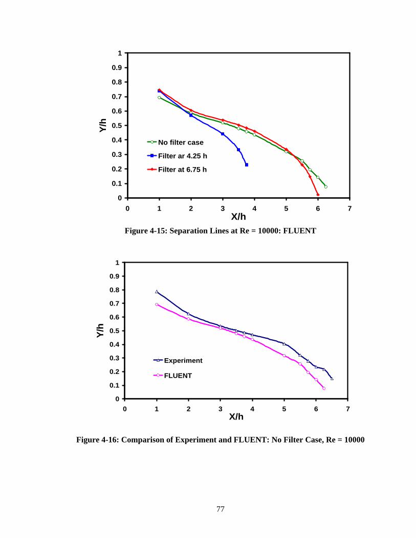
77
0
0.1
0.2
0.3
0.4
0.5
0.6
0.7
0.8
0.9
1
0 1 2 3 4 5 6 7X/h
Y/h
No filter case
Filter ar 4.25 h
Filter at 6.75 h
Figure 4-15: Separation Lines at Re = 10000: FLUENT
0
0.1
0.2
0.3
0.4
0.5
0.6
0.7
0.8
0.9
1
0 1 2 3 4 5 6 7X/h
Y/h
Experiment
FLUENT
Figure 4-16: Comparison of Experiment and FLUENT: No Filter Case, Re = 10000
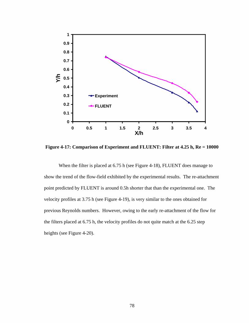
78
0
0.1
0.2
0.3
0.4
0.5
0.6
0.7
0.8
0.9
1
0 0.5 1 1.5 2 2.5 3 3.5 4X/h
Y/h
Experiment
FLUENT
Figure 4-17: Comparison of Experiment and FLUENT: Filter at 4.25 h, Re = 10000
When the filter is placed at 6.75 h (see Figure 4-18), FLUENT does manage to
show the trend of the flow-field exhibited by the experimental results. The re-attachment
point predicted by FLUENT is around 0.5h shorter that than the experimental one. The
velocity profiles at 3.75 h (see Figure 4-19), is very similar to the ones obtained for
previous Reynolds numbers. However, owing to the early re-attachment of the flow for
the filters placed at 6.75 h, the velocity profiles do not quite match at the 6.25 step
heights (see Figure 4-20).
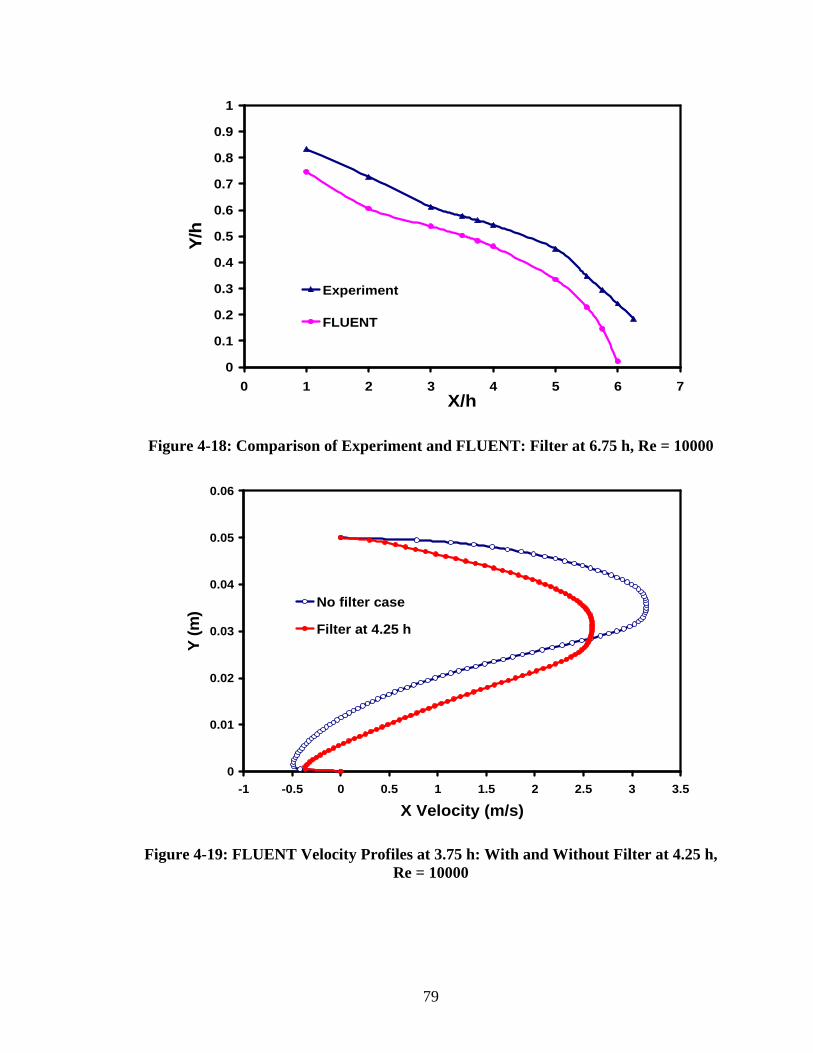
79
0
0.1
0.2
0.3
0.4
0.5
0.6
0.7
0.8
0.9
1
0 1 2 3 4 5 6 7X/h
Y/h
Experiment
FLUENT
Figure 4-18: Comparison of Experiment and FLUENT: Filter at 6.75 h, Re = 10000
0
0.01
0.02
0.03
0.04
0.05
0.06
-1 -0.5 0 0.5 1 1.5 2 2.5 3 3.5
X Velocity (m/s)
Y (
m)
No filter case
Filter at 4.25 h
Figure 4-19: FLUENT Velocity Profiles at 3.75 h: With and Without Filter at 4.25 h, Re = 10000
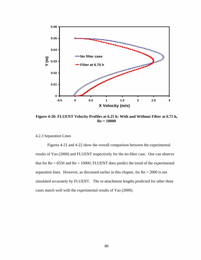
80
0
0.01
0.02
0.03
0.04
0.05
0.06
-0.5 0 0.5 1 1.5 2 2.5 3
X Velocity (m/s)
Y (
m) No filter case
Filter at 6.75 h
Figure 4-20: FLUENT Velocity Profiles at 6.25 h: With and Without Filter at 6.75 h, Re = 10000
4.2.3 Separation Lines
Figures 4-21 and 4-22 show the overall comparison between the experimental
results of Yao (2000) and FLUENT respectively for the no-filter case. One can observe
that for Re = 6550 and Re = 10000, FLUENT does predict the trend of the experimental
separation lines. However, as discussed earlier in this chapter, for Re = 2000 is not
simulated accurately by FLUENT. The re-attachment lengths predicted for other three
cases match well with the experimental results of Yao (2000).
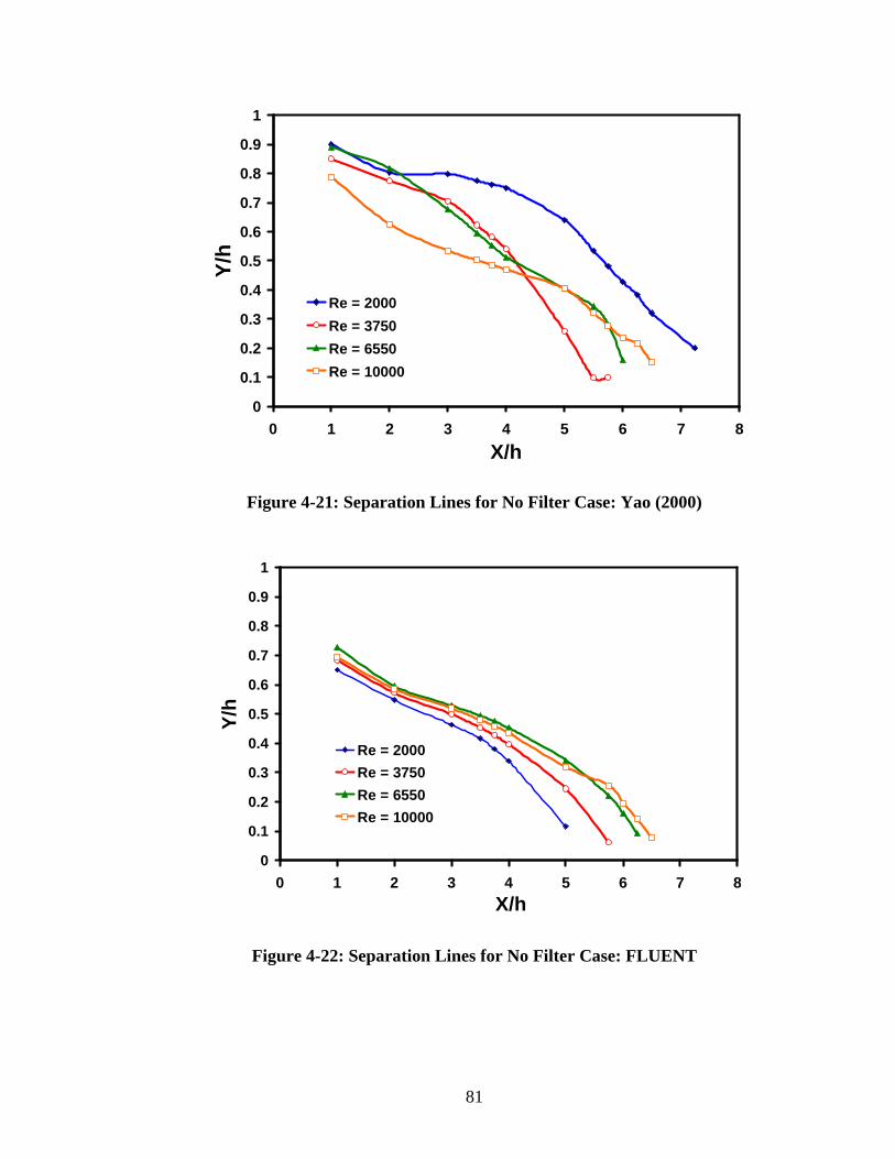
81
0
0.1
0.2
0.3
0.4
0.5
0.6
0.7
0.8
0.9
1
0 1 2 3 4 5 6 7 8
X/h
Y/h
Re = 2000
Re = 3750
Re = 6550
Re = 10000
Figure 4-21: Separation Lines for No Filter Case: Yao (2000)
0
0.1
0.2
0.3
0.4
0.5
0.6
0.7
0.8
0.9
1
0 1 2 3 4 5 6 7 8
X/h
Y/h
Re = 2000
Re = 3750
Re = 6550
Re = 10000
Figure 4-22: Separation Lines for No Filter Case: FLUENT
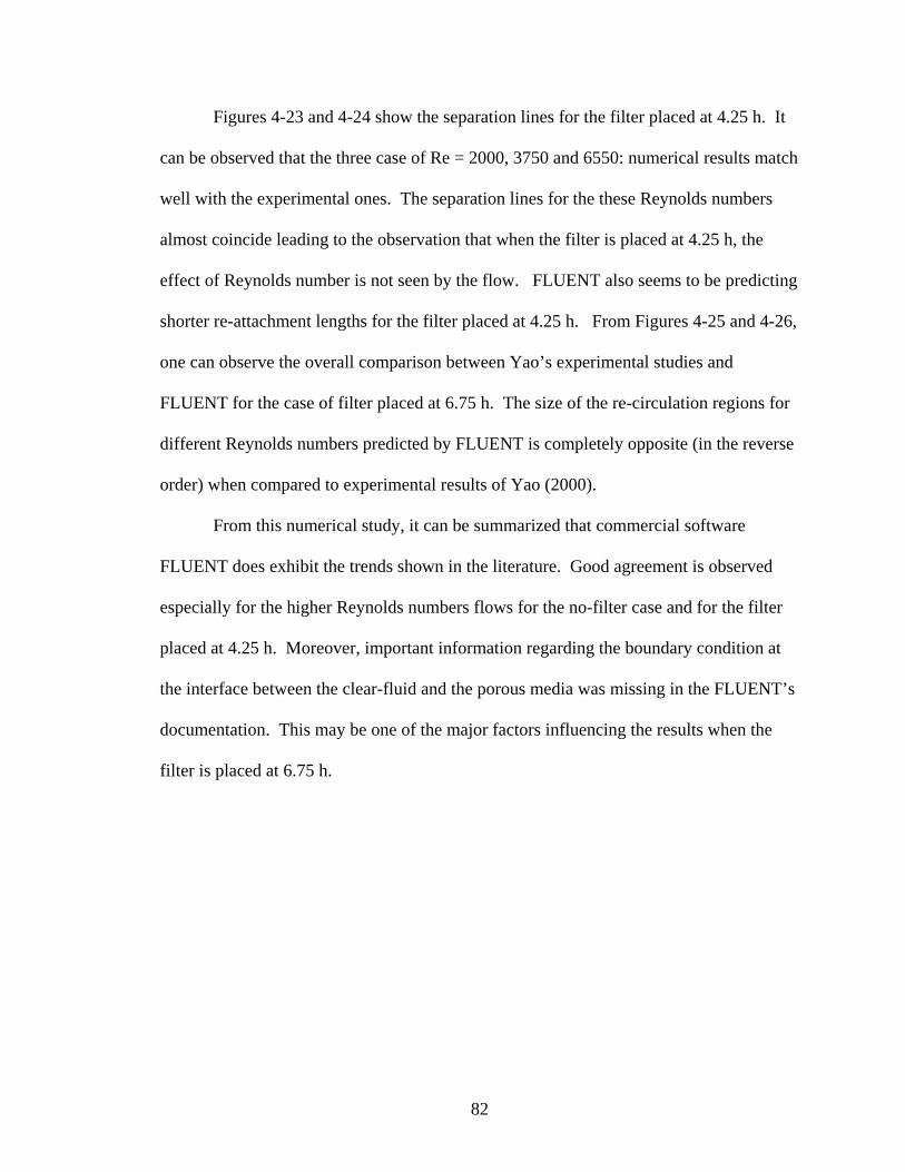
82
Figures 4-23 and 4-24 show the separation lines for the filter placed at 4.25 h. It
can be observed that the three case of Re = 2000, 3750 and 6550: numerical results match
well with the experimental ones. The separation lines for the these Reynolds numbers
almost coincide leading to the observation that when the filter is placed at 4.25 h, the
effect of Reynolds number is not seen by the flow. FLUENT also seems to be predicting
shorter re-attachment lengths for the filter placed at 4.25 h. From Figures 4-25 and 4-26,
one can observe the overall comparison between Yao’s experimental studies and
FLUENT for the case of filter placed at 6.75 h. The size of the re-circulation regions for
different Reynolds numbers predicted by FLUENT is completely opposite (in the reverse
order) when compared to experimental results of Yao (2000).
From this numerical study, it can be summarized that commercial software
FLUENT does exhibit the trends shown in the literature. Good agreement is observed
especially for the higher Reynolds numbers flows for the no-filter case and for the filter
placed at 4.25 h. Moreover, important information regarding the boundary condition at
the interface between the clear-fluid and the porous media was missing in the FLUENT’s
documentation. This may be one of the major factors influencing the results when the
filter is placed at 6.75 h.
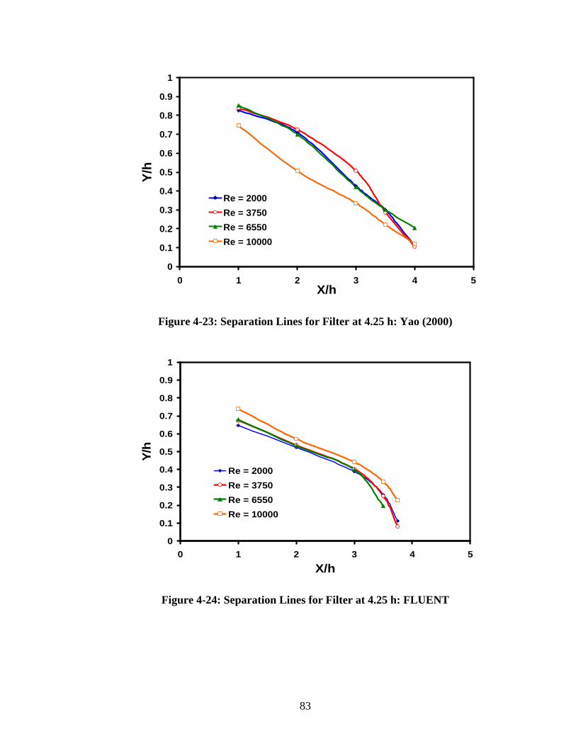
83
0
0.1
0.2
0.3
0.4
0.5
0.6
0.7
0.8
0.9
1
0 1 2 3 4 5X/h
Y/h
Re = 2000
Re = 3750
Re = 6550
Re = 10000
Figure 4-23: Separation Lines for Filter at 4.25 h: Yao (2000)
0
0.1
0.2
0.3
0.4
0.5
0.6
0.7
0.8
0.9
1
0 1 2 3 4 5
X/h
Y/h
Re = 2000
Re = 3750
Re = 6550
Re = 10000
Figure 4-24: Separation Lines for Filter at 4.25 h: FLUENT
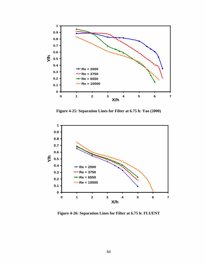
84
0
0.1
0.2
0.3
0.4
0.5
0.6
0.7
0.8
0.9
1
0 1 2 3 4 5 6 7X/h
Y/h
Re = 2000
Re = 3750
Re = 6550
Re = 10000
Figure 4-25: Separation Lines for Filter at 6.75 h: Yao (2000)
0
0.1
0.2
0.3
0.4
0.5
0.6
0.7
0.8
0.9
1
0 1 2 3 4 5 6 7
X/h
Y/h
Re = 2000
Re = 3750
Re = 6550
Re = 10000
Figure 4-26: Separation Lines for Filter at 6.75 h: FLUENT
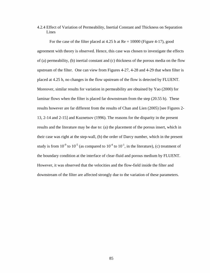
85
4.2.4 Effect of Variation of Permeability, Inertial Constant and Thickness on Separation Lines
For the case of the filter placed at 4.25 h at Re = 10000 (Figure 4-17), good
agreement with theory is observed. Hence, this case was chosen to investigate the effects
of (a) permeability, (b) inertial constant and (c) thickness of the porous media on the flow
upstream of the filter. One can view from Figures 4-27, 4-28 and 4-29 that when filter is
placed at 4.25 h, no changes in the flow upstream of the flow is detected by FLUENT.
Moreover, similar results for variation in permeability are obtained by Yao (2000) for
laminar flows when the filter is placed far downstream from the step (20.55 h). These
results however are far different from the results of Chan and Lien (2005) [see Figures 2-
13, 2-14 and 2-15] and Kuznetsov (1996). The reasons for the disparity in the present
results and the literature may be due to: (a) the placement of the porous insert, which in
their case was right at the step-wall, (b) the order of Darcy number, which in the present
study is from 10-9 to 10-5 (as compared to 10-4 to 10-1, in the literature), (c) treatment of
the boundary condition at the interface of clear-fluid and porous medium by FLUENT.
However, it was observed that the velocities and the flow-field inside the filter and
downstream of the filter are affected strongly due to the variation of these parameters.
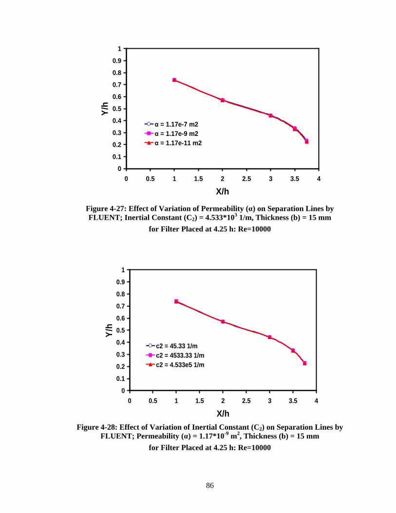
86
0
0.1
0.2
0.3
0.4
0.5
0.6
0.7
0.8
0.9
1
0 0.5 1 1.5 2 2.5 3 3.5 4
X/h
Y/h
α = 1.17e-7 m2α = 1.17e-9 m2α = 1.17e-11 m2
Figure 4-27: Effect of Variation of Permeability (α) on Separation Lines by FLUENT; Inertial Constant (C 2) = 4.533*103 1/m, Thickness (b) = 15 mm
for Filter Placed at 4.25 h: Re=10000
Effect of variation in Inertial constant
0
0.1
0.2
0.3
0.4
0.5
0.6
0.7
0.8
0.9
1
0 0.5 1 1.5 2 2.5 3 3.5 4
X/h
Y/h
c2 = 45.33 1/mc2 = 4533.33 1/mc2 = 4.533e5 1/m
Figure 4-28: Effect of Variation of Inertial Constant (C2) on Separation Lines by
FLUENT; Permeability (α) = 1.17*10-9 m2, Thickness (b) = 15 mm
for Filter Placed at 4.25 h: Re=10000
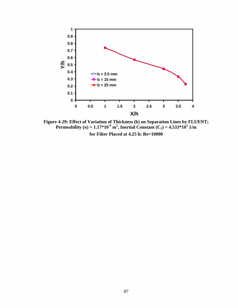
87
0
0.1
0.2
0.3
0.4
0.5
0.6
0.7
0.8
0.9
1
0 0.5 1 1.5 2 2.5 3 3.5 4
X/h
Y/h
b = 3.5 mmb = 15 mmb = 25 mm
Figure 4-29: Effect of Variation of Thickness (b) on Separation Lines by FLUENT;
Permeability (α) = 1.17*10-9 m2, Inertial Constant (C2) = 4.533*103 1/m
for Filter Placed at 4.25 h: Re=10000
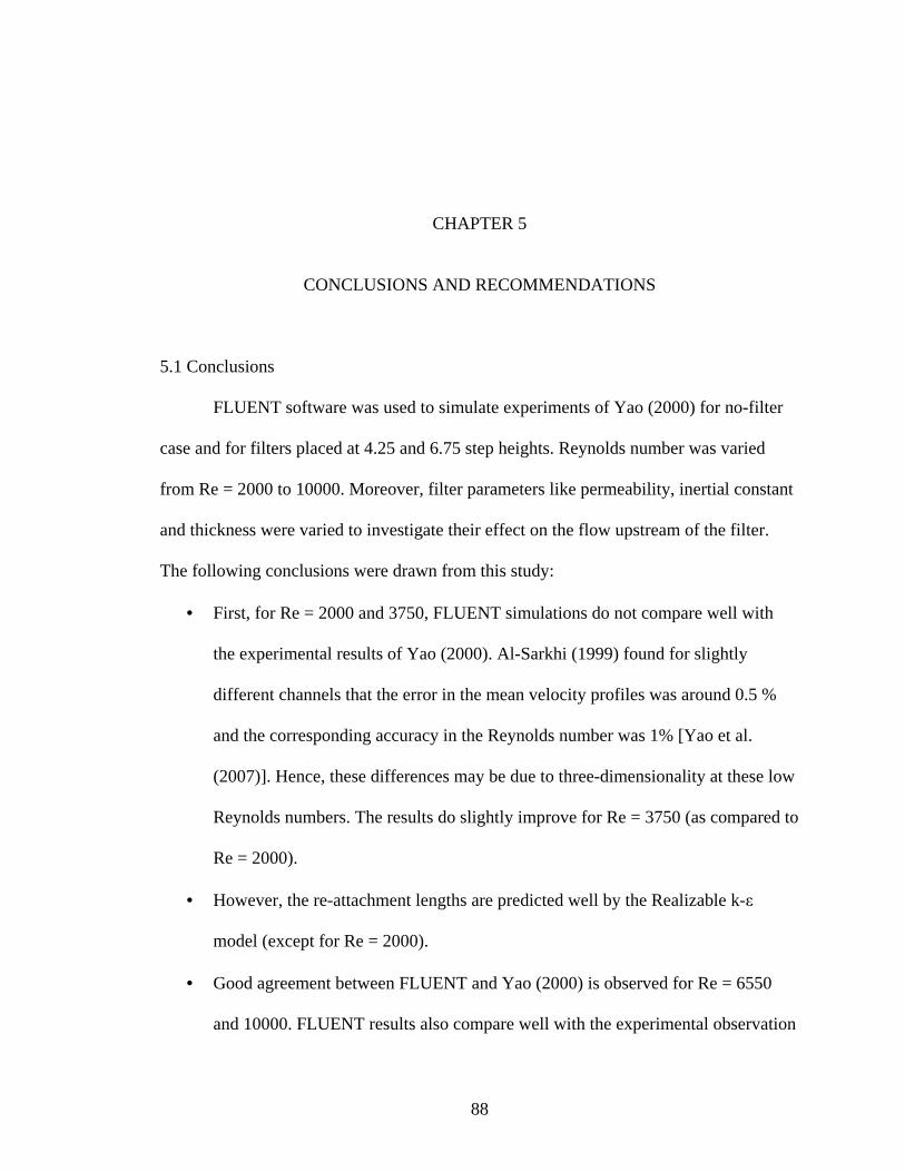
88
CHAPTER 5
CONCLUSIONS AND RECOMMENDATIONS
5.1 Conclusions
FLUENT software was used to simulate experiments of Yao (2000) for no-filter
case and for filters placed at 4.25 and 6.75 step heights. Reynolds number was varied
from Re = 2000 to 10000. Moreover, filter parameters like permeability, inertial constant
and thickness were varied to investigate their effect on the flow upstream of the filter.
The following conclusions were drawn from this study:
• First, for Re = 2000 and 3750, FLUENT simulations do not compare well with
the experimental results of Yao (2000). Al-Sarkhi (1999) found for slightly
different channels that the error in the mean velocity profiles was around 0.5 %
and the corresponding accuracy in the Reynolds number was 1% [Yao et al.
(2007)]. Hence, these differences may be due to three-dimensionality at these low
Reynolds numbers. The results do slightly improve for Re = 3750 (as compared to
Re = 2000).
• However, the re-attachment lengths are predicted well by the Realizable k-ε
model (except for Re = 2000).
• Good agreement between FLUENT and Yao (2000) is observed for Re = 6550
and 10000. FLUENT results also compare well with the experimental observation
89
• of Armaly et al. (1983) for the case of Re = 7000.Thus FLUENT is able to capture
the physics of the re-circulation region to a better extent at higher turbulent
Reynolds numbers. The velocity profiles obtained from FLUENT, compared at
Re = 6550 and 10000 also re-affirm the trend shown in Yao’s experiments.
• Finally, when the filter is placed at 4.25 h, at Re = 10000, the variation of
permeability (from 1.17*10-7 to 1.17*10-11 m2), inertial constant (4.533*101 to
4.533*106 1/m) and thickness of the filter (from 3.5 mm to 25 mm) have no effect
on the re-circulation region upstream of the filter. These may be due to various
reasons as discussed in Section 4.2.4.
5.2 Recommendations
• A good low Reynolds number model that uses a damping function to limit the
turbulence for better simulations at Re = 2000 and 3750 is recommended for
future study.
• Testing for grid-independence for wall-function approach was found to be
cumbersome. Further research using a two-layer approach might be preferable
over wall-functions
• Moreover, the skewness (∆y: ∆x) of some of the grids used in the present study
were almost 1:10. This might result in errors that are related to the advection
terms in the N-S equations especially in the calculation of X-velocity. However,
FLUENT and GAMBIT both considered the present skewness to be within their
operating limits. Hence, finer grids along the X-direction can be investigated in
future.

90
• Commercial CFD software FLUENT has not been extensively used in modeling
porous media. By modifying the modeling constants from the standard values to
values found in the current literature deeper insight can be gained for turbulent
flows through porous media and for flows over backward facing step preceding
porous media.
• Further study using different combinations of wall-functions and various models
will enable us to decide the best combination (of model and wall-function) for
flows with porous inserts.
• Further elucidation on the boundary Condition that FLUENT uses at the interface
of clear-fluid and filter would be appreciated.
• Spalart-Allmaras model could be tested and compared to k-ε models and it might
be a good compromise between desired accuracy and simplicity.
• The need for more detailed and thorough experimentation on flows with porous
inserts would be appreciated in future research.
91
REFERENCES
Adams EW, Eaton JK. 1988. An LDA study of the backward facing step flow, including the effects of velocity bias. Journal of Fluids Engineering 110:275-82
AIAA Guide for the verification and validation of computational fluid dynamics
simulations. 1998. AIAA-G-077 Al-Sarkhi A. 1999. Optimization technique for design of automotive air-filter housing
with improved fluid dynamic performance. PhD Thesis, Oklahoma State University, Stillwater, OK, USA
Alvarez G, Bournet PE, Flick D. 2003. Two-dimensional simulation of turbulent flow
and heat transfer through packed spheres. International Journal of Heat and Mass Transfer 46:2459-69
Antohe BV, Lage JL. 1997. A general two-equation macroscopic turbulence model for
incompressible flow in porous media. International Journal of Heat and Mass Transfer 40:3013-24
Armaly BF, Durst F, Pereira JCF, Schönung B. 1983. Experimental and theoretical
investigation of backward facing step flow. Journal of Fluid Mechanics 127:473-96
Armaly BF, Li A, Nie JH. 2003. Measurements in three-dimensional laminar separated
flow. International Journal of Heat and Mass Transfer 46:3573-82 Assato M, Pedras MHJ, deLemos MJS. 2005. Numerical solution of turbulent channel
flow past a backward facing step with a porous insert using linear and non-linear k-e models. Journal of Porous Media 8:13-29
Avremenko AA, Kuznetsov AV. 2006. Renormalization group model for large-scale
turbulence in porous media. Transport in Porous Media 63:175-93 Beaudoin J-F, Cadot O, Aider J-L, Wesfried JE. 2004. Three-dimensional stationary
flow over a backward facing step. European Journal of Mechanics B/Fluids 23:147-55
92
Behamadouche S, Jarrin N, Addad Y, Laurence D. 2006. Synthetic turbulent inflow conditions based on a vortex method for large-eddy simulation. Progress in Computational Fluid Dynamics 6:50-7
Benedict LH, Gould RD. 1998. Near wall velocity measurements in the recirculation
zone of a backwards facing step flow. 1998 ASME Fluids Engineering Division Summer Meeting, pp. 1-8. Washington DC, USA
Biswas G, Breuer M, Durst F. 2004. Backward facing step flows for various expansion
ratios at low and moderate Reynolds numbers. Transactions of ASME Journal 126:362-74
Braza M, Minh HH, Cazalbou JB. 1984. Numerical analysis of laminar flow over a step.
Notes on Numerical Fluid Mechanics 9:97-113 Bredberg J, Peng SH, Davidson L. 2002. An improved k-w model applied to
recirculating flows. International Journal of Heat and Fluid Flow 23:731-43 Camussi R, Guj G, Di Marco A, Ragni A. 2006. Propagation of wall pressure
perturbations in a large aspect ratio shallow cavity. Experiments in Fluids 40:612-20
Celik IB, Li J. 2005. Assessment of numerical uncertainty for the calculations of
turbulent flow over a backward facing step. International Journal for Numerical Methods in Fluids 49:1015-31
Chan EC, Lien FS. 2005. Permeability effects of turbulent flow through a porous insert
in a backward facing step channel. Transport in Porous Media 59:47-71 Chandesris M, Serre G, Sagaut P. 2006. A macroscopic turbulence model for flow in
porous media suited for pipe and rod bundle flows. International Journal of Heat and Mass Transfer 49:2739-50
Chen F, Chen CF. 1992. Convection in superposed fluid and porous layers. Journal of
Fluid Mechanics 234:97-119 Chiang TP, Sheu TWH. 1999. A numerical revisit of backward-facing step flow
problem. Physics of Fluids 11: 862-74 Chung K, Lee KS, Kim WS. 2003. Modified macroscopic turbulence modeling for the
tube with channel geometry in porous media. Numerical Heat Transfer A: 659-68
Craft TJ, Launder BE, Suga K. 1996. Development and application of cubic eddy-
viscosity model of turbulence. International Journal of Heat and Mass Transfer 17:108-15
93
Darcy H. 1856. Les fontaines publiques de la ville de Dijon. Dalmont, Paris. Dejoan A, Jang YJ, Leschziner MA. 2004. LES and unsteady RANS computations for a
periodically perturbed separated flow over a backward-facing step. 2004 ASME Heat Transfer/ Fluids Engineering Summer Conference, pp. HT-FED04-56211. Charlotte, North Carolina, USA
Driver D, Seegmiller HL. 1985. Features of a reattaching turbulent shear layer in
divergent channel flow. AIAA Journal 23:163-71 Durbin PA. 1995. Separation computations with k-ε-v2 model. AIAA Journal 33:633-5 Durst F, Tropea C. 1981. Turbulent backward facing step flows in two-dimensional
ducts and channels. Third International Symposium on Turbulent Shear Flows, pp. 18.1-5. University of California, Davis, CA, USA
Dybbs A, Edwards RV. 1984. A new look at porous media fluid mechanics: Darcy to
turbulent. NATO ASI Series 82:199-256 Eaton JK, Johnston, JP. 1980. Turbulent flow reattachment: An experimental study of
the flow and structure behind a backward facing step, Rep.MD-39, Thermo-Sciences Division, Department of Mechanical Engineering, Stanford University
Ecer A, Rout RK, Ward P. 1984. Laminar flow past a backward facing step. Notes on
Numerical Fluid Mechanics 9:213-29 Editorial Policy Statement on Numerical and Experimental Accuracy. Journal of
Guidance, Control and Dynamics 30: 9 FLUENT 6.1 User’s Guide. 2003. FLUENT, Inc. Lebanon, NH, USA FLUENT 6.1 User’s Guide. 2003. FLUENT, Inc., On the WWW URL
http://www.fluent.com (July 31, 2007) Furuichi N, Hachiga T, Kumada M. 2004. An experimental investigation of a large-
scale structure of a two-dimensional backward-facing step by using advanced multi-point LDV. Experiments in Fluids 36:274-81
Furuichi N, Kumada M. 2002. An experimental study of a span wise structure around a
reattachment region of a two-dimensional backward facing step. Experiments in Fluids 32:179-87
Getachew D, Mincowycz WJ, Lage JL. 2000. A modified form of k-ε model for
turbulent flows of an incompressible fluid in porous media. International Journal of Heat and Mass Transfer 43:2909-15
94
Goussibaile J, Huaguel A, Hervouet JM. 1984. Calculation of flow over a backward facing step. Notes on Numerical Fluid Mechanics 9:268-89
Gualtieri C. 2005. Numerical simulation of laminar backward facing step flow with
FEMLAB 3.1. 2005 ASME Fluids Engineering Division Summer Meeting and Exhibition, pp. FEDSM2005-77314. Houston, TX, USA
Gullbrand J, Wirtz RA. 2005. Comparison of LES and RANS simulation of turbulent
convection in structured porous media. 2005 ASME Heat Transfer Conference. San-Francisco, California, USA
Hall SD, Behnia M, Fletcher CAJ, Morrison GL. 2003. Investigation of the secondary
corner vortex in a benchmark turbulent backward facing step using cross correlation particle imaging velocimetry. Experiments in Fluids 35:139-51
Hanjalic K, Launder BE. 1972. A Reynolds stress model of turbulence and its
application to thin shearing flows. Journal of Fluid Mechanics 52:609-38 Hudy LM, Naguib AM. 2005. Particle imaging velocimetry measurements of a
two/three dimensional separating/reattaching boundary layer downstream of an axisymmetric backward-facing step. 43rd AIAA Aerospace Sciences Meeting and Exhibit. Reno, Nevada, USA
Inagaki M, Kondoh T, Nagano Y. 2005. A mixed-time-scale SGS model with fixed
model-parameters for practical LES. Journal of Fluids Engineering 127:1-13 Isomoto K, Honami S. 1989. The effect of inlet turbulent intensity on the reattachment
process over a backward facing step. Journal of Fluids Engineering 111:87-92 Jovic S, Driver D. 1994. Backward-facing step measurement at low Reynolds numbers.
Rep. NASA TM 108807, NASA Jovic S, Driver DM. 1995. Reynolds number effects on the skin friction in the separated
flows behind a backward facing step flow. Experiments in Fluids 18:464-7 Kaiktsis L, Karniadakis GE, Orszag SA. 1991. Onset of three-dimensionality,
equilibrium and early transition in flow over a backward-facing step. Journal of Fluid Mechanics 231:501-28
Kanna PR, Das MK. 2006. A short note on the reattachment length for BFS problem.
International Journal for Numerical Methods in Fluids 50:683-92 Ke F, Liu YZ, Wang WZ, Chen HP. 2006. Wall pressure fluctuations of turbulent flow
over backward facing step with and without entrainment: Microphone array measurement. Journal of Hydrodynamics 18:383-96
95
Kim J, Moin P. 1986. Structure of the vorticity field in turbulent channel flow. Part 2. Study of ensemble-averaged fields. Journal of Fluid Mechanics 162:339-63
Kim JY, Ghajar AJ, Tang C, Foutch GL. 2005. Comparison of near-wall treatment
methods foe high Reynolds number backward-facing step flow. International Journal of Computational Fluid Dynamics 19:493-500
Kostas J, Soria J, Chong MS. 2002. Particle image velocimetry measurements of a
backward-facing step flow. Experiments in Fluids 33:838–53
Kuznetsov AV. 1996. Analytical investigation of the fluid flow in the interface region between a porous medium and a clear fluid in channels partially filled with a porous medium. Applied Scientific Research 56: 53-62
Launder BE, Sharma BI. 1974. Application of the energy-dissipation model of turbulence
to the calculation of flow near a spinning disc. Letters in Heat Mass Transfer 1: 131-38
Launder BE, Spalding DB. 1974. The numerical computation of turbulent flows.
Computational Methods and Applications of Mechanical Engineering 3:269-89 Le H, Moin P, Kim J. 1997. Direct numerical simulation of turbulent flow over a
backward facing step flow. Journal of Fluid Mechanics 330:349-74 Lee I, Ahn SK, Sung HJ. 2004. Three-dimensional coherent structure in a separated and
reattaching flow over a backward facing step. Experiments in Fluids 36:373-83 Lee I, Sung HJ. 2002. Multiple arrayed pressure measurement for investigation of the
unsteady flow structure of a reattaching shear layer. Journal of Fluid Mechanics 463:377-402
Lee K, Howell JR. 1987. Forced convective and radiative transfer with in a highly
porous layer exposed to a turbulent external flow field. Proceedings of 1987 ASME-JSME Thermal Engineering Joint Conference, pp. 377-86
Lee T, Mateescu D. 1998. Experimental and numerical investigation of 2-D backward
facing step flow. Journal of Fluids and Structures 12:703-16 Masuoka T, Takatsu Y. 1996. Turbulence model for flow through porous media.
International Journal of Heat and Mass Transfer 39:2803-9 Masuoka T, Takatsu Y. 2005. Transition process to turbulent flow in porous media.
Proceedings of 2005 ASME International Mechanical Engineering Congress Exposition. Orlando, Florida, USA
96
Masuoka T, Takatsu Y, Inoue T. 2002. Chaotic behavior and Transition to turbulence in porous media. Journal of Porous Media 1:243-51
Menter FR. 1994. Two-equation eddy-viscosity turbulence models for engineering
applications. AIAA Journal 32: 1598-1605 Moser RD, Kim J, Mansour NN. 1999. Direct numerical simulation of turbulent channel
flow up to Reτ = 590. Physics of Fluids 11:943-5 Nakayama A, Kuwahara F. 1999. A macroscopic turbulence model for flow in porous
medium. Journal of Fluids Engineering 121:427-33 Neumann J, Wengle H. 2003. DNS and LES of passively controlled turbulent
backward-facing step flow. Flow, Turbulence and Combustion 71: 297–310 Newman RA. 1995. Uniformity of air flow in automotive test housing and its effects on
the efficiency of fibrous filters. MS Thesis, Oklahoma State University, Stillwater, OK, USA
Ochoa-Tapia JA, Whitaker S. 1995. Momentum transfer at the boundary between a
porous medium and a homogeneous fluid-II: Comparison with experiment. International Journal of Heat and Mass Transfer 38:2647-55
Pedras MHJ, deLemos MJS. 2001. Macroscopic turbulence modeling for
incompressible flow through undeformable porous media. International Journal of Heat and Mass Transfer 44:1081-93
Pedras MHJ, deLemos MJS. 2003. Computation of turbulent flow in porous media
using a low-Reynolds k-e model and an infinite array of transversally displaced elliptic rods. Numerical Heat Transfer, Part A, Applications 43:585-602
Petry AP, Awruch AM. 2006. Large eddy simulation of three dimensional turbulent
flows by the finite element method. Associação Brasileira de Ciências Mecânicas XXVIII: 224-32
Piirto M, Saarenrinne P, Eloranta H, Karvinen R. 2003. Measuring turbulence energy
with PIV in a backward-facing step flow. Experiments in Fluids 35:219–36 Pilloni MT, Schram C, Riethmuller ML. 2000. PIV and LDV measurements behind a
backward facing step. Advances in Air Pollution Series 8:633-42 Pope SB. 2000. Turbulent Flows: Cambridge University Press, NY, USA Popiolek TL, Awruch AM, Teixeira PRF. 2006. Finite element analysis of laminar and
turbulent flows using LES and subgrid scale models. Applied Mathematical Modeling 30:177-99
97
Roache PJ. 2002. Code verification by the method of manufactured solutions. Journal of Fluids Engineering 124: 4-10
Saric S, Jakirlic S, Tropea C. 2005. A periodically perturbed backward facing step flow
by means of LES, DES and T-RANS: An example of flow separation and control. Journal of Fluids Engineering 127:879-85
Schlichting H. 1979. Boundary layer theory. New York, NY: McGraw-Hill Seguin D, Montillet A, Comiti J. 1998. Experimental Characterization of regimes in
various porous media - I: Limit of laminar flow regime. Chemical Engineering Science 53:3751-61
Seguin D, Montillet A, Comiti J, Huet P. 1998. Experimental Characterization of
regimes in various porous media - II: Transition to turbulent regime. Chemical Engineering Science 53:3897-909
Shih TS, Zhu J, Lumley JL. 1994. Calculation of wall bounded complex flows and free
shear flows. International Journal for Numerical Methods in Fluids 23:1133-44 Silveira NA, Grand D, Metais O, Lesieur M. 1991. Large-eddy simulation of the
turbulent flow in the downstream region of a backward facing step. Physical Review Letters 66:2320-7
Sinha SN, Gupta AK, Oberai MM. 1981. Laminar separating flows over backsteps and
cavities part I: backsteps. AIAA Journal 19:1527-30 Speziale CG. 1987. On non-linear k-e models of turbulence. Journal of Fluid
Mechanics 178:459-75 Stephano GD, Denaro FM, Ricardi G. 1998. Analysis of 3D backward facing step
incompressible flows via a local average based numerical procedure. International Journal of Numerical Methods for Fluids 28:1073-91
Takatsu Y, Masuoka T. 1998. Turbulent Phenomena in Flow through Porous Media.
Journal of Porous Media 1:243-52 Tebutt, CB. 1995. CFD model of flow through air filter pleats. MS Thesis, Oklahoma
State University, Stillwater, OK, USA Toumi A, Phouc LT, Daube O. 1984. Calculation of flow over a backward facing step.
Notes on Numerical Fluid Mechanics 9:405-20 Tylli N, Kaiktsis L, Ineichen B. 2002. Sidewall effects in flow over a backward-facing
step: Experiments and numerical simulation. Physics of Fluids 14:3835-45
98
Valsecchi P. 2005. Numerical investigation of shear-layer instabilities using temporal and spatial DNS. 43rd AIAA Aerospace Sciences Meeting & Exhibit, pp. 13007-17. Reno, Nevada, USA
Wengle H, Huppertz A, Bärwolff G, Janke G. 2001. The manipulated transitional
backward-facing step flow: an experimental and direct numerical simulation investigation. European Journal of Mechanics - B/Fluids 20:25–46
Whitaker S. 1984. Flow in porous media I: A theoretical derivation of Darcy's law.
Transport in Porous Media 1:3-25 Wilcox DC. 1998. Turbulence Modeling for CFD. DCW Industries, Inc. La Canãda, CA,
USA Williams PT, Baker AJ. 1997. Numerical simulations of laminar flow over a 3D
backward facing step. International Journal of Numerical Methods for Fluids 24:1159 -83
Yakhot V, Orszag SA. 1986. Renormalization group analysis of turbulence- I: Basic
theory Journal of Scientific Computing 1:3-51 Yang XD, Ma XY, Huang YN. 2003. Prediction of homogenous shear flow and
backward facing step flow with some linear and non-linear k-e turbulence models. Communications in Non-Linear Science and Numerical Simulation 10:315-28
Yao SH. 2000. Two dimensional backward facing step flows preceding an automotive
air filter . PhD Thesis, Oklahoma State University, Stillwater, OK, USA Yao SH, Krishnamoorthy C, Chambers FW. 2007. Experiments on backward-facing
step preceding a porous medium. 5th Joint ASME/JSME Fluids Engineering Conference, pp. FEDSM2007-37204. San Diego, California USA.
Yoshizawa A, Nisizima S. 1993. Non-equilibrium representation of turbulent viscosity
based on two-scale turbulence theory. Physics of Fluids A: 3302-4
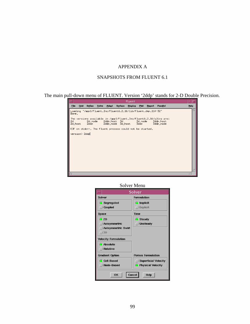
99
APPENDIX A
SNAPSHOTS FROM FLUENT 6.1
The main pull-down menu of FLUENT. Version ‘2ddp’ stands for 2-D Double Precision.
Solver Menu
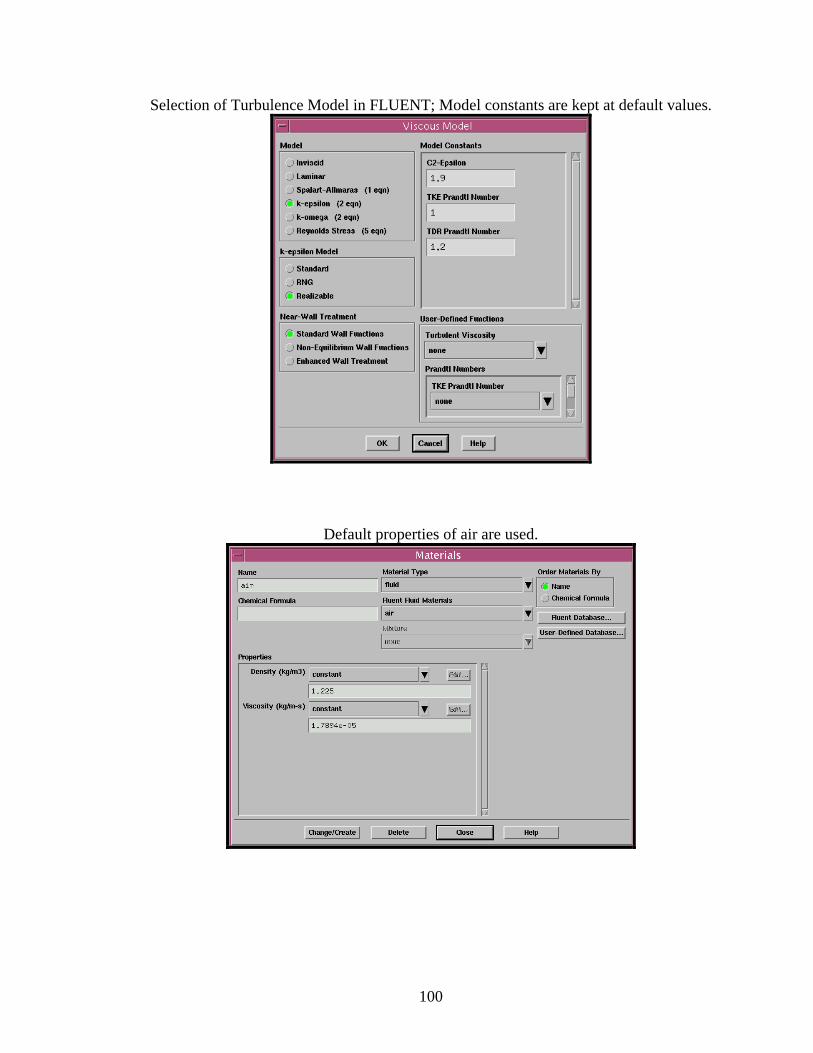
100
Selection of Turbulence Model in FLUENT; Model constants are kept at default values.
Default properties of air are used.
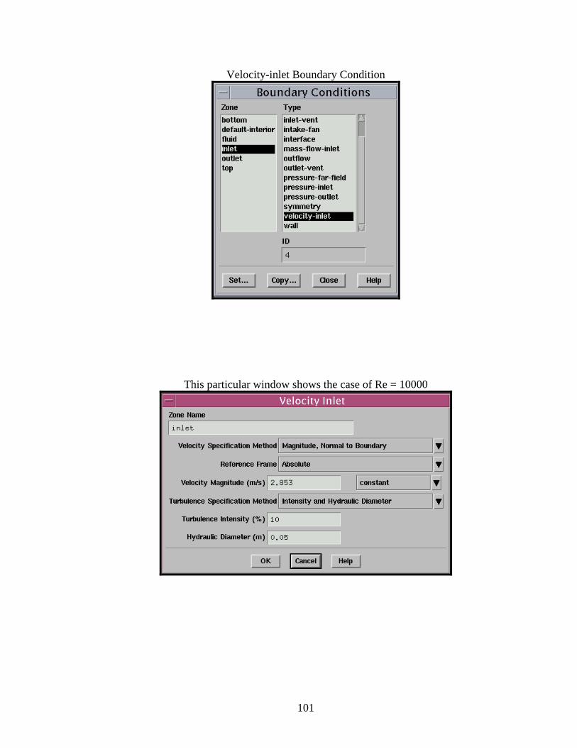
101
Velocity-inlet Boundary Condition
This particular window shows the case of Re = 10000
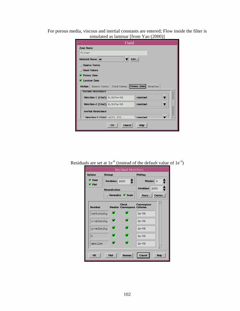
102
For porous media, viscous and inertial constants are entered; Flow inside the filter is simulated as laminar [from Yao (2000)]
Residuals are set at 1e-6 (instead of the default value of 1e-3)
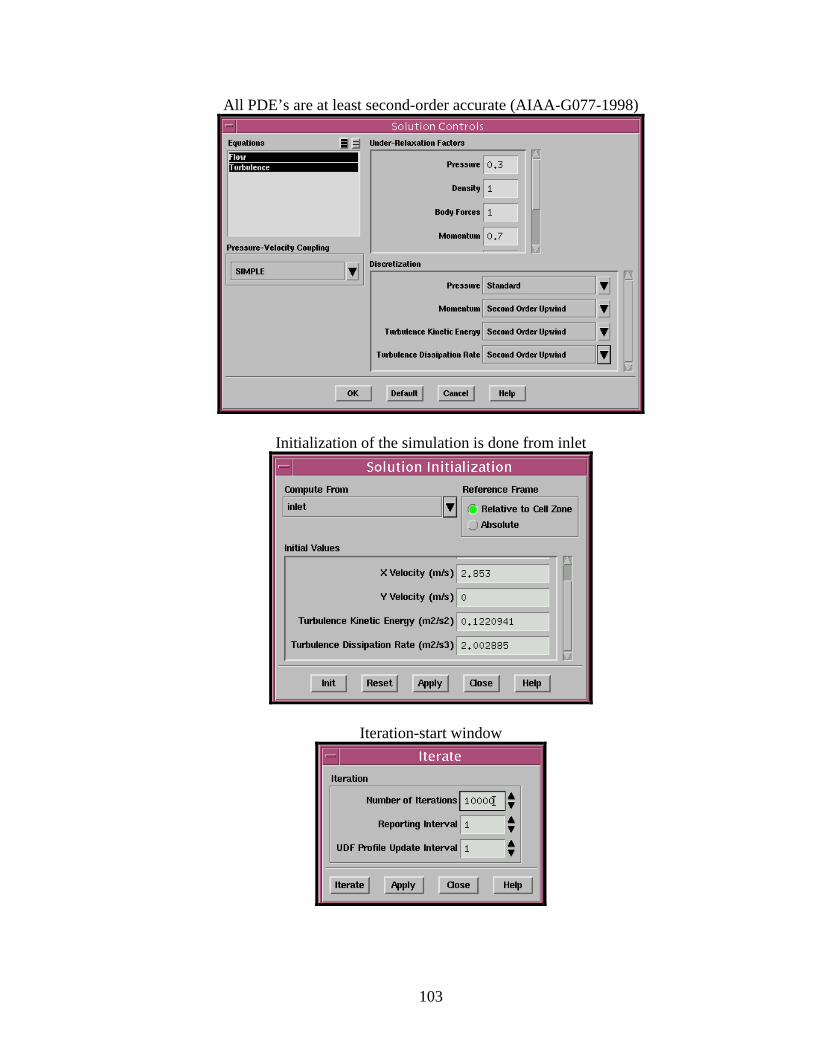
103
All PDE’s are at least second-order accurate (AIAA-G077-1998)
Initialization of the simulation is done from inlet
Iteration-start window
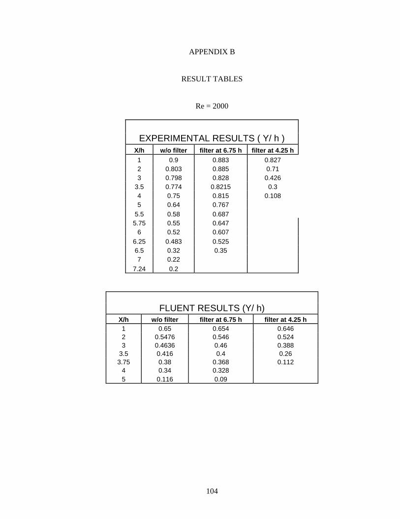
104
APPENDIX B
RESULT TABLES
Re = 2000
FLUENT RESULTS (Y/ h) X/h w/o filter filter at 6.75 h filter at 4.25 h 1 0.65 0.654 0.646 2 0.5476 0.546 0.524 3 0.4636 0.46 0.388
3.5 0.416 0.4 0.26 3.75 0.38 0.368 0.112
4 0.34 0.328 5 0.116 0.09
EXPERIMENTAL RESULTS ( Y/ h ) X/h w/o filter filter at 6.75 h filter at 4.25 h 1 0.9 0.883 0.827 2 0.803 0.885 0.71 3 0.798 0.828 0.426
3.5 0.774 0.8215 0.3 4 0.75 0.815 0.108 5 0.64 0.767
5.5 0.58 0.687 5.75 0.55 0.647
6 0.52 0.607 6.25 0.483 0.525 6.5 0.32 0.35 7 0.22
7.24 0.2
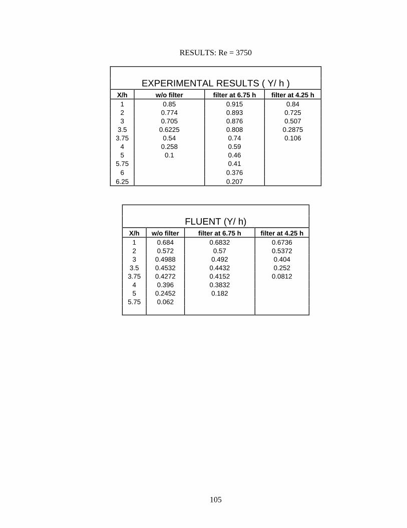
105
RESULTS: Re = 3750
EXPERIMENTAL RESULTS ( Y/ h ) X/h w/o filter filter at 6.75 h filter at 4.25 h 1 0.85 0.915 0.84 2 0.774 0.893 0.725 3 0.705 0.876 0.507
3.5 0.6225 0.808 0.2875 3.75 0.54 0.74 0.106
4 0.258 0.59 5 0.1 0.46
5.75 0.41 6 0.376
6.25 0.207
FLUENT (Y/ h) X/h w/o filter filter at 6.75 h filter at 4.25 h 1 0.684 0.6832 0.6736 2 0.572 0.57 0.5372 3 0.4988 0.492 0.404
3.5 0.4532 0.4432 0.252 3.75 0.4272 0.4152 0.0812
4 0.396 0.3832 5 0.2452 0.182
5.75 0.062
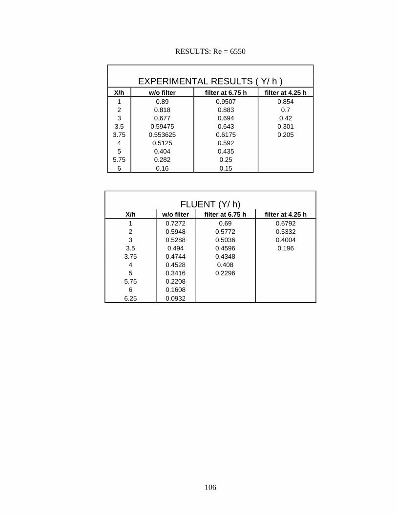
106
RESULTS: Re = 6550
EXPERIMENTAL RESULTS ( Y/ h ) X/h w/o filter filter at 6.75 h filter at 4.25 h 1 0.89 0.9507 0.854 2 0.818 0.883 0.7 3 0.677 0.694 0.42
3.5 0.59475 0.643 0.301 3.75 0.553625 0.6175 0.205
4 0.5125 0.592 5 0.404 0.435
5.75 0.282 0.25 6 0.16 0.15
FLUENT (Y/ h) X/h w/o filter filter at 6.75 h filter at 4.25 h 1 0.7272 0.69 0.6792 2 0.5948 0.5772 0.5332 3 0.5288 0.5036 0.4004
3.5 0.494 0.4596 0.196 3.75 0.4744 0.4348
4 0.4528 0.408 5 0.3416 0.2296
5.75 0.2208 6 0.1608
6.25 0.0932
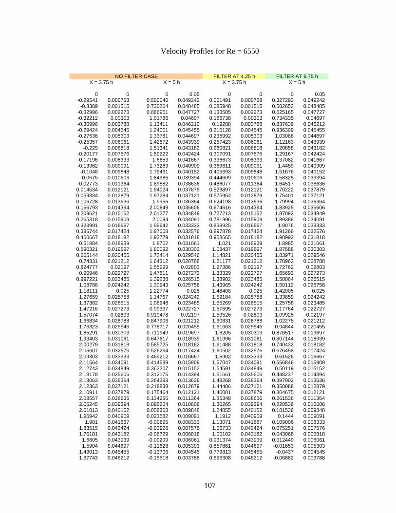
107
Velocity Profiles for Re = 6550
NO FILTER CASE FILTER AT 4.25 h FILTER AT 6.75 h X = 3.75 h X = 5 h X = 3.75 h X = 5 h
0 0 0 0.05 0 0 0 0.05
-0.29541 0.000758 0.500046 0.049242 0.001491 0.000758 0.327293 0.049242 -0.3309 0.001515 0.730264 0.048485 0.085948 0.001515 0.502653 0.048485
-0.32996 0.002273 0.886951 0.047727 0.133585 0.002273 0.625165 0.047727 -0.32212 0.00303 1.01786 0.04697 0.166738 0.00303 0.734335 0.04697 -0.30996 0.003788 1.13411 0.046212 0.19288 0.003788 0.837636 0.046212 -0.29424 0.004545 1.24001 0.045455 0.215128 0.004545 0.936309 0.045455 -0.27536 0.005303 1.33781 0.044697 0.235992 0.005303 1.03088 0.044697 -0.25357 0.006061 1.42872 0.043939 0.257423 0.006061 1.12163 0.043939
-0.229 0.006818 1.51341 0.043182 0.280821 0.006818 1.20858 0.043182 -0.20177 0.007576 1.59222 0.042424 0.307091 0.007576 1.29167 0.042424 -0.17196 0.008333 1.6653 0.041667 0.336673 0.008333 1.37082 0.041667 -0.13962 0.009091 1.73269 0.040909 0.369611 0.009091 1.4459 0.040909
-0.1048 0.009848 1.79431 0.040152 0.405693 0.009848 1.51676 0.040152 -0.0675 0.010606 1.84986 0.039394 0.444609 0.010606 1.58325 0.039394
-0.02773 0.011364 1.89882 0.038636 0.486077 0.011364 1.64517 0.038636 0.014534 0.012121 1.94024 0.037879 0.529897 0.012121 1.70222 0.037879 0.059334 0.012879 1.97284 0.037121 0.575954 0.012879 1.75401 0.037121 0.106728 0.013636 1.9956 0.036364 0.624198 0.013636 1.79994 0.036364 0.156793 0.014394 2.00849 0.035606 0.674616 0.014394 1.83925 0.035606 0.209621 0.015152 2.01277 0.034849 0.727213 0.015152 1.87092 0.034849 0.265318 0.015909 2.0094 0.034091 0.781996 0.015909 1.89388 0.034091 0.323991 0.016667 1.99642 0.033333 0.838925 0.016667 1.9076 0.033333 0.385744 0.017424 1.97008 0.032576 0.897878 0.017424 1.91266 0.032576 0.450667 0.018182 1.92779 0.031818 0.958665 0.018182 1.90992 0.031818
0.51884 0.018939 1.8702 0.031061 1.021 0.018939 1.8985 0.031061 0.590321 0.019697 1.80092 0.030303 1.08437 0.019697 1.87588 0.030303 0.665144 0.020455 1.72414 0.029546 1.14821 0.020455 1.83971 0.029546
0.74331 0.021212 1.64312 0.028788 1.21177 0.021212 1.78962 0.028788 0.824777 0.02197 1.55999 0.02803 1.27386 0.02197 1.72762 0.02803
0.90946 0.022727 1.47611 0.027273 1.33329 0.022727 1.65693 0.027273 0.997221 0.023485 1.39238 0.026515 1.38902 0.023485 1.58064 0.026515
1.08786 0.024242 1.30943 0.025758 1.43965 0.024242 1.50112 0.025758 1.18111 0.025 1.22774 0.025 1.48408 0.025 1.42005 0.025 1.27659 0.025758 1.14767 0.024242 1.52184 0.025758 1.33859 0.024242 1.37382 0.026515 1.06948 0.023485 1.55269 0.026515 1.25758 0.023485 1.47216 0.027273 0.99337 0.022727 1.57695 0.027273 1.17764 0.022727 1.57074 0.02803 0.919478 0.02197 1.59526 0.02803 1.09925 0.02197 1.66834 0.028788 0.847906 0.021212 1.60831 0.028788 1.02275 0.021212 1.76323 0.029546 0.778717 0.020455 1.61663 0.029546 0.94844 0.020455 1.85291 0.030303 0.711949 0.019697 1.6205 0.030303 0.876517 0.019697 1.93403 0.031061 0.647617 0.018939 1.61996 0.031061 0.807144 0.018939 2.00279 0.031818 0.585725 0.018182 1.61488 0.031818 0.740432 0.018182 2.05607 0.032576 0.526264 0.017424 1.60502 0.032576 0.676458 0.017424 2.09303 0.033333 0.469212 0.016667 1.5902 0.033333 0.61526 0.016667 2.11564 0.034091 0.414539 0.015909 1.57047 0.034091 0.556846 0.015909 2.12743 0.034849 0.362207 0.015152 1.54591 0.034849 0.50119 0.015152 2.13178 0.035606 0.312175 0.014394 1.51661 0.035606 0.448237 0.014394 2.13063 0.036364 0.264398 0.013636 1.48268 0.036364 0.397903 0.013636 2.12363 0.037121 0.218838 0.012879 1.44406 0.037121 0.350088 0.012879 2.10911 0.037879 0.175464 0.012121 1.40081 0.037879 0.304675 0.012121 2.08557 0.038636 0.134256 0.011364 1.35348 0.038636 0.261536 0.011364 2.05245 0.039394 0.095204 0.010606 1.30265 0.039394 0.220536 0.010606 2.01013 0.040152 0.058308 0.009848 1.24855 0.040152 0.181536 0.009848 1.95942 0.040909 0.023582 0.009091 1.1912 0.040909 0.1444 0.009091
1.901 0.041667 -0.00895 0.008333 1.13071 0.041667 0.109006 0.008333 1.83515 0.042424 -0.03926 0.007576 1.06733 0.042424 0.075251 0.007576 1.76181 0.043182 -0.06729 0.006818 1.00102 0.043182 0.043068 0.006818
1.6805 0.043939 -0.09299 0.006061 0.931374 0.043939 0.012449 0.006061 1.5904 0.044697 -0.11628 0.005303 0.857861 0.044697 -0.01653 0.005303
1.49013 0.045455 -0.13706 0.004545 0.779813 0.045455 -0.0437 0.004545 1.37743 0.046212 -0.15518 0.003788 0.696308 0.046212 -0.06882 0.003788
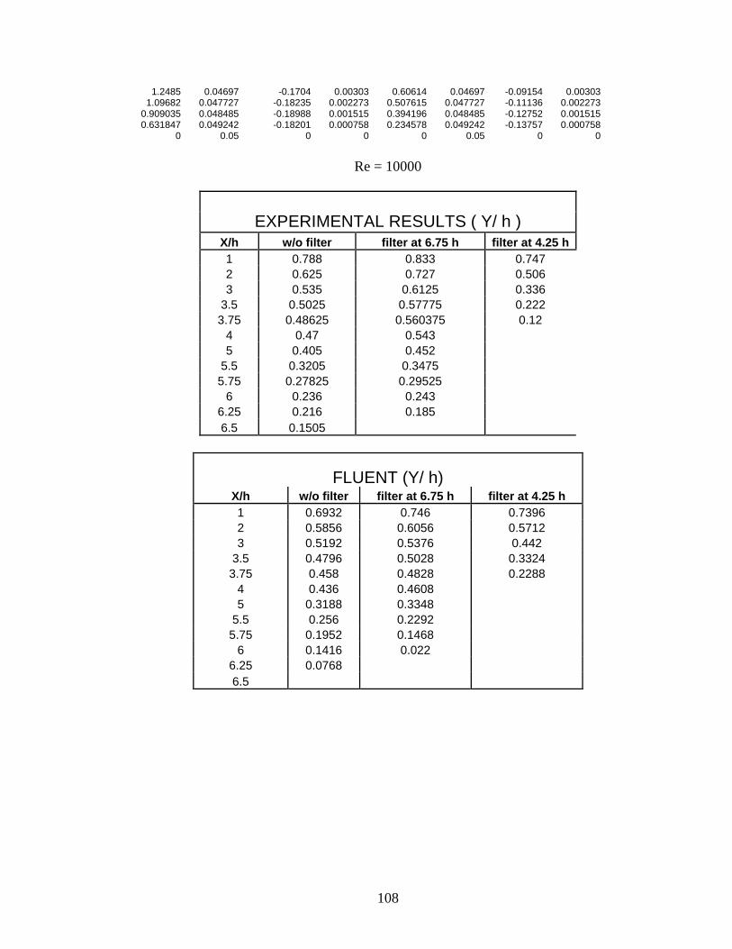
108
1.2485 0.04697 -0.1704 0.00303 0.60614 0.04697 -0.09154 0.00303 1.09682 0.047727 -0.18235 0.002273 0.507615 0.047727 -0.11136 0.002273
0.909035 0.048485 -0.18988 0.001515 0.394196 0.048485 -0.12752 0.001515 0.631847 0.049242 -0.18201 0.000758 0.234578 0.049242 -0.13757 0.000758
0 0.05 0 0 0 0.05 0 0
Re = 10000
EXPERIMENTAL RESULTS ( Y/ h ) X/h w/o filter filter at 6.75 h filter at 4.25 h 1 0.788 0.833 0.747 2 0.625 0.727 0.506 3 0.535 0.6125 0.336
3.5 0.5025 0.57775 0.222 3.75 0.48625 0.560375 0.12
4 0.47 0.543 5 0.405 0.452
5.5 0.3205 0.3475 5.75 0.27825 0.29525
6 0.236 0.243 6.25 0.216 0.185 6.5 0.1505
FLUENT (Y/ h) X/h w/o filter filter at 6.75 h filter at 4.25 h 1 0.6932 0.746 0.7396 2 0.5856 0.6056 0.5712 3 0.5192 0.5376 0.442
3.5 0.4796 0.5028 0.3324 3.75 0.458 0.4828 0.2288
4 0.436 0.4608 5 0.3188 0.3348
5.5 0.256 0.2292 5.75 0.1952 0.1468
6 0.1416 0.022 6.25 0.0768 6.5
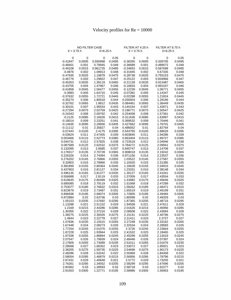
109
Velocity profiles for Re = 10000
NO FILTER CASE FILTER AT 4.25 h FILTER AT 6.75 h X = 3.75 h
X=6.25 h
X = 3.75 h
X=6.25 h
0 0 0 0.05 0 0 0 0.05
-0.41847 0.0005 0.550998 0.0495 -0.36355 0.0005 0.335705 0.0495 -0.48401 0.001 0.79945 0.049 -0.36689 0.001 0.489072 0.049 -0.49108 0.0015 0.961725 0.0485 -0.34653 0.0015 0.587698 0.0485
-0.4876 0.002 1.08913 0.048 -0.31945 0.002 0.67335 0.048 -0.47935 0.0025 1.19878 0.0475 -0.28738 0.0025 0.755153 0.0475 -0.46776 0.003 1.29822 0.047 -0.25122 0.003 0.834966 0.047 -0.45353 0.0035 1.39119 0.0465 -0.21139 0.0035 0.913487 0.0465 -0.43705 0.004 1.47967 0.046 -0.16833 0.004 0.991037 0.046 -0.41858 0.0045 1.56477 0.0455 -0.12239 0.0045 1.06771 0.0455
-0.3983 0.005 1.64715 0.045 -0.07381 0.005 1.14347 0.045 -0.37632 0.0055 1.72721 0.0445 -0.02288 0.0055 1.21824 0.0445 -0.35274 0.006 1.80518 0.044 0.030004 0.006 1.29196 0.044 -0.32762 0.0065 1.8812 0.0435 0.084461 0.0065 1.36449 0.0435 -0.30101 0.007 1.95534 0.043 0.140154 0.007 1.43571 0.043 -0.27294 0.0075 2.02759 0.0425 0.196771 0.0075 1.50547 0.0425 -0.24343 0.008 2.09792 0.042 0.254008 0.008 1.57361 0.042
-0.2125 0.0085 2.16626 0.0415 0.311636 0.0085 1.63997 0.0415 -0.18014 0.009 2.23251 0.041 0.369532 0.009 1.70446 0.041 -0.14635 0.0095 2.29656 0.0405 0.427662 0.0095 1.76701 0.0405 -0.11112 0.01 2.35827 0.04 0.486052 0.01 1.82764 0.04 -0.07443 0.0105 2.4175 0.0395 0.544755 0.0105 1.88629 0.0395 -0.03624 0.011 2.47405 0.039 0.603845 0.011 1.94286 0.039 0.003466 0.0115 2.52773 0.0385 0.663404 0.0115 1.99727 0.0385 0.044731 0.012 2.57825 0.038 0.723518 0.012 2.04946 0.038 0.087589 0.0125 2.62532 0.0375 0.784272 0.0125 2.09941 0.0375 0.132095 0.013 2.6685 0.037 0.845747 0.013 2.14708 0.037 0.178317 0.0135 2.70728 0.0365 0.908018 0.0135 2.19242 0.0365 0.226326 0.014 2.74094 0.036 0.971156 0.014 2.23537 0.036 0.276202 0.0145 2.76866 0.0355 1.03522 0.0145 2.27587 0.0355
0.32803 0.015 2.78966 0.035 1.10025 0.015 2.31385 0.035 0.381899 0.0155 2.80364 0.0345 1.16628 0.0155 2.34915 0.0345 0.437903 0.016 2.81127 0.034 1.23331 0.016 2.38148 0.034 0.496135 0.0165 2.81377 0.0335 1.30127 0.0165 2.41041 0.0335 0.556688 0.017 2.8119 0.033 1.37009 0.017 2.43554 0.033 0.619645 0.0175 2.80499 0.0325 1.43982 0.0175 2.45646 0.0325 0.685085 0.018 2.79119 0.032 1.51068 0.018 2.47289 0.032 0.753077 0.0185 2.76832 0.0315 1.58262 0.0185 2.48471 0.0315 0.823679 0.019 2.73487 0.031 1.65519 0.019 2.49199 0.031 0.896938 0.0195 2.69074 0.0305 1.72805 0.0195 2.49484 0.0305 0.972884 0.02 2.63736 0.03 1.80099 0.02 2.49329 0.03
1.05153 0.0205 2.57692 0.0295 1.87365 0.0205 2.48716 0.0295 1.13288 0.021 2.51152 0.029 1.94558 0.021 2.47611 0.029
1.2169 0.0215 2.44286 0.0285 2.01626 0.0215 2.45956 0.0285 1.30355 0.022 2.37216 0.028 2.08508 0.022 2.43694 0.028 1.39275 0.0225 2.30026 0.0275 2.15131 0.0225 2.40796 0.0275
1.4844 0.023 2.22778 0.027 2.21411 0.023 2.3727 0.027 1.57836 0.0235 2.15515 0.0265 2.27248 0.0235 2.33162 0.0265 1.67448 0.024 2.08273 0.026 2.32534 0.024 2.28583 0.026 1.77254 0.0245 2.01076 0.0255 2.3726 0.0245 2.23664 0.0255 1.87228 0.025 1.93944 0.025 2.41532 0.025 2.18465 0.025 1.97338 0.0255 1.86894 0.0245 2.45299 0.0255 2.13019 0.0245 2.07547 0.026 1.79939 0.024 2.48446 0.026 2.07397 0.024 2.17809 0.0265 1.73089 0.0235 2.51011 0.0265 2.01676 0.0235 2.28068 0.027 1.66352 0.023 2.53072 0.027 1.95921 0.023 2.38255 0.0275 1.59735 0.0225 2.54698 0.0275 1.90173 0.0225 2.48286 0.028 1.53242 0.022 2.55969 0.028 1.84458 0.022 2.58054 0.0285 1.46879 0.0215 2.56956 0.0285 1.78796 0.0215 2.67431 0.029 1.40648 0.021 2.5772 0.029 1.73205 0.021 2.76261 0.0295 1.34552 0.0205 2.58299 0.0295 1.67696 0.0205 2.84362 0.03 1.28593 0.02 2.58718 0.03 1.62277 0.02 2.91553 0.0305 1.22771 0.0195 2.58986 0.0305 1.56953 0.0195
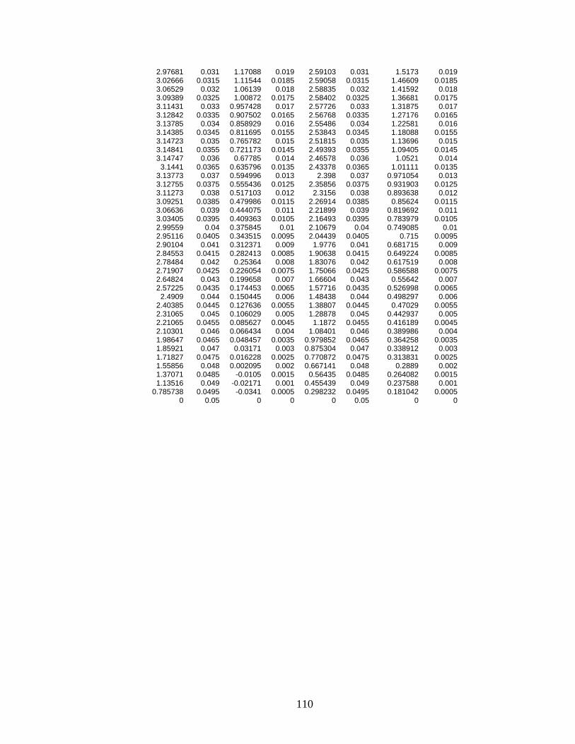
110
2.97681 0.031 1.17088 0.019 2.59103 0.031 1.5173 0.019 3.02666 0.0315 1.11544 0.0185 2.59058 0.0315 1.46609 0.0185 3.06529 0.032 1.06139 0.018 2.58835 0.032 1.41592 0.018 3.09389 0.0325 1.00872 0.0175 2.58402 0.0325 1.36681 0.0175 3.11431 0.033 0.957428 0.017 2.57726 0.033 1.31875 0.017 3.12842 0.0335 0.907502 0.0165 2.56768 0.0335 1.27176 0.0165 3.13785 0.034 0.858929 0.016 2.55486 0.034 1.22581 0.016 3.14385 0.0345 0.811695 0.0155 2.53843 0.0345 1.18088 0.0155 3.14723 0.035 0.765782 0.015 2.51815 0.035 1.13696 0.015 3.14841 0.0355 0.721173 0.0145 2.49393 0.0355 1.09405 0.0145 3.14747 0.036 0.67785 0.014 2.46578 0.036 1.0521 0.014
3.1441 0.0365 0.635796 0.0135 2.43378 0.0365 1.01111 0.0135 3.13773 0.037 0.594996 0.013 2.398 0.037 0.971054 0.013 3.12755 0.0375 0.555436 0.0125 2.35856 0.0375 0.931903 0.0125 3.11273 0.038 0.517103 0.012 2.3156 0.038 0.893638 0.012 3.09251 0.0385 0.479986 0.0115 2.26914 0.0385 0.85624 0.0115 3.06636 0.039 0.444075 0.011 2.21899 0.039 0.819692 0.011 3.03405 0.0395 0.409363 0.0105 2.16493 0.0395 0.783979 0.0105 2.99559 0.04 0.375845 0.01 2.10679 0.04 0.749085 0.01 2.95116 0.0405 0.343515 0.0095 2.04439 0.0405 0.715 0.0095 2.90104 0.041 0.312371 0.009 1.9776 0.041 0.681715 0.009 2.84553 0.0415 0.282413 0.0085 1.90638 0.0415 0.649224 0.0085 2.78484 0.042 0.25364 0.008 1.83076 0.042 0.617519 0.008 2.71907 0.0425 0.226054 0.0075 1.75066 0.0425 0.586588 0.0075 2.64824 0.043 0.199658 0.007 1.66604 0.043 0.55642 0.007 2.57225 0.0435 0.174453 0.0065 1.57716 0.0435 0.526998 0.0065
2.4909 0.044 0.150445 0.006 1.48438 0.044 0.498297 0.006 2.40385 0.0445 0.127636 0.0055 1.38807 0.0445 0.47029 0.0055 2.31065 0.045 0.106029 0.005 1.28878 0.045 0.442937 0.005 2.21065 0.0455 0.085627 0.0045 1.1872 0.0455 0.416189 0.0045 2.10301 0.046 0.066434 0.004 1.08401 0.046 0.389986 0.004 1.98647 0.0465 0.048457 0.0035 0.979852 0.0465 0.364258 0.0035 1.85921 0.047 0.03171 0.003 0.875304 0.047 0.338912 0.003 1.71827 0.0475 0.016228 0.0025 0.770872 0.0475 0.313831 0.0025 1.55856 0.048 0.002095 0.002 0.667141 0.048 0.2889 0.002 1.37071 0.0485 -0.0105 0.0015 0.56435 0.0485 0.264082 0.0015 1.13516 0.049 -0.02171 0.001 0.455439 0.049 0.237588 0.001
0.785738 0.0495 -0.0341 0.0005 0.298232 0.0495 0.181042 0.0005 0 0.05 0 0 0 0.05 0 0
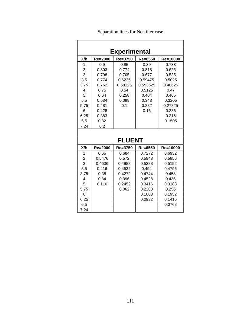
111
Separation lines for No-filter case
Experimental X/h Re=2000 Re=3750 Re=6550 Re=10000 1 0.9 0.85 0.89 0.788 2 0.803 0.774 0.818 0.625 3 0.798 0.705 0.677 0.535
3.5 0.774 0.6225 0.59475 0.5025 3.75 0.762 0.58125 0.553625 0.48625
4 0.75 0.54 0.5125 0.47 5 0.64 0.258 0.404 0.405
5.5 0.534 0.099 0.343 0.3205 5.75 0.481 0.1 0.282 0.27825
6 0.428 0.16 0.236 6.25 0.383 0.216 6.5 0.32 0.1505 7.24 0.2
FLUENT X/h Re=2000 Re=3750 Re=6550 Re=10000 1 0.65 0.684 0.7272 0.6932 2 0.5476 0.572 0.5948 0.5856 3 0.4636 0.4988 0.5288 0.5192
3.5 0.416 0.4532 0.494 0.4796 3.75 0.38 0.4272 0.4744 0.458
4 0.34 0.396 0.4528 0.436 5 0.116 0.2452 0.3416 0.3188
5.75 0.062 0.2208 0.256 6 0.1608 0.1952
6.25 0.0932 0.1416 6.5 0.0768 7.24
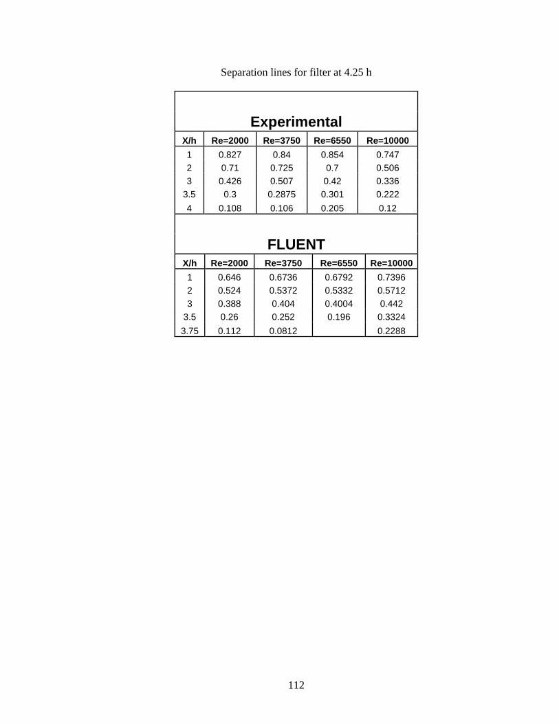
112
Separation lines for filter at 4.25 h
Experimental X/h Re=2000 Re=3750 Re=6550 Re=10000
1 0.827 0.84 0.854 0.747 2 0.71 0.725 0.7 0.506 3 0.426 0.507 0.42 0.336
3.5 0.3 0.2875 0.301 0.222
4 0.108 0.106 0.205 0.12
FLUENT X/h Re=2000 Re=3750 Re=6550 Re=10000
1 0.646 0.6736 0.6792 0.7396 2 0.524 0.5372 0.5332 0.5712 3 0.388 0.404 0.4004 0.442
3.5 0.26 0.252 0.196 0.3324
3.75 0.112 0.0812 0.2288
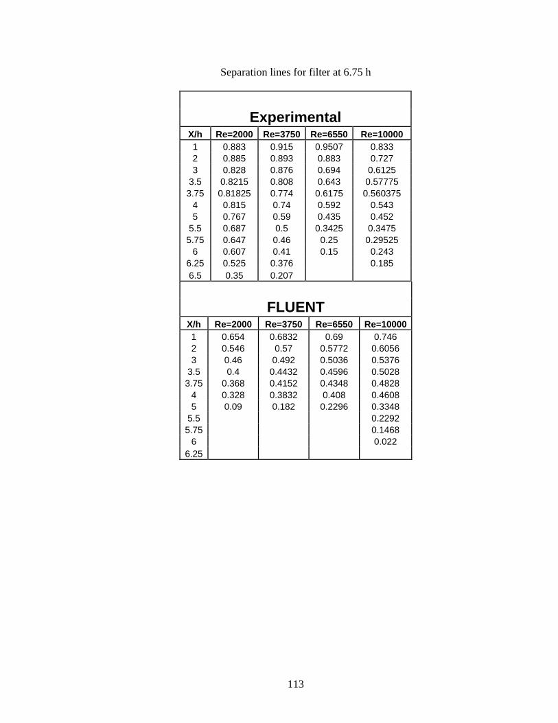
113
Separation lines for filter at 6.75 h
Experimental X/h Re=2000 Re=3750 Re=6550 Re=10000 1 0.883 0.915 0.9507 0.833 2 0.885 0.893 0.883 0.727 3 0.828 0.876 0.694 0.6125
3.5 0.8215 0.808 0.643 0.57775 3.75 0.81825 0.774 0.6175 0.560375
4 0.815 0.74 0.592 0.543 5 0.767 0.59 0.435 0.452
5.5 0.687 0.5 0.3425 0.3475 5.75 0.647 0.46 0.25 0.29525
6 0.607 0.41 0.15 0.243 6.25 0.525 0.376 0.185 6.5 0.35 0.207
FLUENT X/h Re=2000 Re=3750 Re=6550 Re=10000 1 0.654 0.6832 0.69 0.746 2 0.546 0.57 0.5772 0.6056 3 0.46 0.492 0.5036 0.5376
3.5 0.4 0.4432 0.4596 0.5028 3.75 0.368 0.4152 0.4348 0.4828
4 0.328 0.3832 0.408 0.4608 5 0.09 0.182 0.2296 0.3348
5.5 0.2292 5.75 0.1468
6 0.022 6.25
VITA
CHANDRAMOULEE KRISHNAMOORTHY
Candidate for the Degree of
Master of Science Thesis: NUMERICAL ANALYSIS OF BACKWARD-FACING STEP PRECEEDING
A POROUS MEDIUM USING FLUENT Major Field: Mechanical and Aerospace Engineering Biographical:
Personal Data: Born in Pondicherry, India, on May 18, 1982, son of K.Kamakshi and V.Krishnamoorthy
Education: Graduated from S.I.W.S. High School and G.N. Khalsa College,
Mumbai, India in March 1998 and May 2000 respectively. Received Bachelor of Engineering (B.E.) degree in Mechanical Engineering from University of Mumbai, Mumbai, India in July 2004. Completed the requirements for the Master of Science degree in Mechanical and Aerospace Engineering at Oklahoma State University in August, 2007
Experience: Graduate Trainee Engineer, from July 2004 to May 2005, Blue
Star Ltd., India. Teaching Assistant, from Aug 2005 to July 2007, Department of Mechanical and Aerospace Engineering, Oklahoma State University.
Professional Memberships: Student Member of American Society of
Mechanical Engineers (ASME), Student Member of American Institute of Aeronautics and Astronautics (AIAA).
Name: Chandramoulee Krishnamoorthy Date of Degree: December, 2007 Institution: Oklahoma State University Location: Stillwater, Oklahoma Title of Study: NUMERICAL ANALYSIS OF BACKWARD-FACING STEP FLOW
PRECEEDING A POROUS MEDIUM USING FLUENT Pages in Study: 113 Candidate for the Degree of Master of Science
Major Field: Mechanical and Aerospace Engineering Scope and Method of Study: The purpose of the present study is to numerically simulate
the flow over a backward-facing step for the no-filter case and for filters at 4.25 and 6.75 step heights. Commercial CFD software FLUENT is used for numerical computations and results are validated with the experimental studies of Yao (2000). The simulations are performed for Reynolds numbers: 2000, 3750, 6550 and 10000. In the present work, GAMBIT software is used for modeling and grid-generation. Different turbulence models in FLUENT namely: Spalart-Allmaras, k-ε models, k-ω models and Reynolds Stress model are tested. Amongst the various models, Realizable k-ε model is chosen and grid-independence studies are carried out. The numerical results from FLUENT are then compared with the experimental results of Yao (2000). Moreover, filter parameters like permeability, inertial constant and thickness are varied for the case of Re = 10000 and filter placed at 4.25 step heights.
Findings and Conclusions: For Re = 2000 and 3750, FLUENT simulations do not
compare well with the experimental results of Yao (2000). The no-filter case at Re = 2000, has a re-attachment length of almost 8 h (step-heights); Turbulent models in FLUENT were unable to simulate this numerically due to transitional nature of the flow at these Reynolds numbers. However, results do slightly improve for Re = 3750. Good agreement between FLUENT and Yao (2000) is observed for Re = 6550 and 10000. Thus FLUENT is able to capture the physics of the re-circulation region to a better extent at higher turbulent Reynolds numbers. The velocity profiles obtained from FLUENT, compared at Re = 6550 and 10000 also re-affirm the trend shown in Yao (2000)’s experiments. Finally, when the filter is placed at 4.25 h, at Re = 10000, the variation of permeability, inertial constant and thickness of the filter have no effect on the re-circulation region upstream of the filter.
ADVISER’S APPROVAL: Frank W. Chambers