Embed Size (px)
Citation preview
INFLUENCE OF BOREHOLE CONSTRUCTION ON
LNAPL THICKNESS MEASUREMENTS
By
JENNIFER L. THORSTAD
Bachelor of Science in Geology
North Dakota State University
Fargo, ND
2005
Submitted to the Faculty of the Graduate College of the
Oklahoma State University in partial fulfillment of the requirements for
the Degree of MASTER OF SCIENCE
May, 2007
INFLUENCE OF BOREHOLE CONSTRUCTION
ON LNAPL THICKNESS MEASUREMENTS
Thesis Approved:
Dr. Todd Halihan Thesis Advisor
Dr. Anna Cruse
Dr. Eliot Atekwana
Dr. A. Gordon Emslie Dean of the Graduate College
ii

ACKNOWLEDGEMENTS
This research would not have been possible without the data provided by
Aestus, LLC, Oklahoma Corporation Commission-Petroleum Storage Tank
Division, and previous research conducted by the School of Geology at
Oklahoma State University. Funding assistance from Devon Energy is also
greatly appreciated.
I am especially grateful to my advisor, Dr. Todd Halihan, for pushing me to
new limits. He provided valuable insight on numerical modeling, contaminant
transport in the subsurface, and geophysical techniques. I also would like to
thank my committee members, Dr. Anna Cruse and Dr. Eliot Atekwana, for
critiquing my writing and always offering advice. Finally, I express my sincere
gratitude to my family and friends for their support.
iii

TABLE OF CONTENTS
Chapter Page I. INTRODUCTION .........................................................................................1
Purpose of Study........................................................................................2 Objectives ..................................................................................................2 Field Sites ..................................................................................................3 Enid, OK..........................................................................................4 Geology......................................................................................5 Field Data...................................................................................6 Golden, OK .....................................................................................8 Geology......................................................................................9 Field Data.................................................................................10 Hobart, OK.....................................................................................13 Geology....................................................................................14 Field Data.................................................................................15 Summary.......................................................................................17 II. REVIEW OF LITERATURE .......................................................................18 Borehole Construction..............................................................................18
Monitoring Wells ............................................................................18 Pumping Wells...............................................................................20 Significant Parameters and Variables ......................................................21 Hydraulic Conductivity...................................................................21 Natural Media................................................................................22 Borehole Construction..............................................................23 Filter Pack ............................................................................23 Annular Seal.........................................................................23 Capillary Pressure and Fluid Saturation .........................................24 van Genuchten Model Parameters............................................24 Two-phase Flow and Wells ......................................................................26 Electrical Resistivity Imaging ...................................................................33 COMSOL Multiphysics .............................................................................36 III. METHODOLOGY .....................................................................................37 Numerical Model Development ................................................................37 Model Geometry ............................................................................37
iv
Governing Equations and Constitutive Relationships……………... 39 Fluid Retention and Permeability ..............................................41 Boundary and Initial Conditions......................................................43 IV. RESULTS.................................................................................................46 Convergent Flow Field .............................................................................46 Sand Aquifer ..................................................................................47 Silty, Clayey Sand Aquifer..............................................................49 Divergent Flow Field ................................................................................50 Sand Aquifer...................................................................................51 Silty, Clayey Sand Aquifer..............................................................53 Borehole Size...........................................................................................55 V. DISCUSSION...........................................................................................57 Comparison of Field and Model Results ..................................................57 Equilibrium Time Scales...........................................................................60 Modeling Limitations ................................................................................61 VI. CONCLUSIONS.......................................................................................63 REFERENCES..............................................................................................65 APPENDIXES................................................................................................70 APPENDIX A – LITHOLOGY AND WELL CONSTRUCTION AT HOBART, OK Site ..........................................................70 APPENDIX B – COMSOL MULTIPHYSICS MODEL ...............................73
v
LIST OF TABLES
Table Page
1.1 Stratigraphy of the Enid, OK site...........................................................6
1.2 Stratigraphy of the Golden, OK site ....................................................10
1.3 Stratigraphy of the Hobart, OK site .....................................................15
1.4 Core data from Hobart, OK site ..........................................................16
1.5 Depth to ground water and LNAPL at Hobart, OK site........................17
2.1 Hydraulic conductivity and instrinsic permeability values for
unconsolidated sediments ..................................................................22
2.2 Hydraulic conductivity values for unfractured rocks ............................22
2.3 van Genuchten parameters ................................................................25
3.1 Parameters used in numerical model .................................................45
vi
LIST OF FIGURES
Figure Page
1.1 Location map of Enid, Golden, and Hobart OK.....................................4
1.2 Location map of monitoring electrode boreholes at Enid, OK site ........5
1.3 ERT compared to TPH along ME 13-10-3 at Enid, OK site ..................7
1.4 LNAPL thickness measurements from wells at Enid, OK site ...............8
1.5 Map of well locations and electrical resistivity lines at Golden, OK site 9
1.6 Electrical resistivity image of subsurface at Golden, OK site ..............11
1.7 ERI taken along line EI-1-EW at Golden, OK site ...............................12
1.8 ERI taken along line EI-2-NS at Golden, OK site................................13
1.9 Map of well locations and electrical resistivity lines at Hobart, OK site14
1.10 ERI of line GS-008 at Hobart, OK site.................................................16
2.1 Construction of monitoring wells .........................................................19
2.2 General configuration of a pumping well.............................................20
2.3 Typical soil moisture characteristic curves..........................................25
2.4 “Pancake layer” conceptualization model ...........................................26
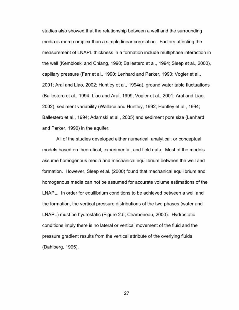
2.5 Phase distribution under static equilibrium conditions between a well and
the natural media .....................................................................................28
3.1 Model geometry in plan view ..............................................................38
3.2 Mesh of model ....................................................................................39
3.3 Boundary conditions for the model aquifer shown in plan view...........44
vii
4.1 Convergent flow field ..........................................................................47
4.2 Saturation of the non-wetting phase at the center of the borehole
(Borehole: K =10-3 m/s; Media: K=10-4 m/s) .............................................48
4.3 Saturation of the non-wetting phase outside of the borehole
(Borehole: K =10-3 m/s; Media: K=10-4 m/s) .............................................48
4.4 Saturation of the non-wetting phase at the center of the borehole
(Borehole: K =10-3 m/s; Media: K=10-6 m/s) .............................................50
4.5 Saturation of the non-wetting phase outside of the borehole
(Borehole: K =10-3 m/s; Media: K=10-6 m/s) .............................................50
4.6 Divergent flow field .............................................................................51
4.7 Saturation of the non-wetting phase in the center of the borehole
(Borehole: K =10-9 m/s; Media: K=10-4 m/s) .............................................52
4.8 Saturation of the non-wetting phase outside of the borehole
(Borehole: K =10-9 m/s; Media: K=10-4 m/s) .............................................53
4.9 Saturation of the non-wetting phase at the center of the borehole
(Borehole: K =10-9 m/s; Media: K=10-6 m/s) .............................................54
4.10 Saturation of the non-wetting phase outside of the borehole
(Borehole: K =10-9 m/s; Media: K=10-6 m/s) .............................................54
4.11 Saturation of the non-wetting phase in the center of 2, 4, and 12 inch
diameter boreholes (Borehole: K=10-3 m/s; Media: K= 10-4 m/s) .............55
4.12 Saturation of the non-wetting phase in the center of 2, 4, and 12 inch
diameter boreholes (Borehole: K=10-9 m/s; Media: K= 10-4 m/s) .............56
5.1 Time to equilibrium during the entry and departure of LNAPL ............61
viii
LIST OF SYMBOLS
Symbol Description Units
α van Genuchten fitting parameter L-1
A Area L2
Cnw Specific capacity of non-wetting fluid Dimensionless
Cp Specific capacity, p denotes pressure LT2 M-1
Cp,nw Specific capacity of non-wetting fluid LT2 M-1
Cp,w Specific capacity of wetting fluid LT2 M-1
Cw Specific capacity of wetting fluid Dimensionless
D Coordinate of vertical elevation L
dh/dL Gradient L L-1
g Acceleration of gravity L T-2
Hc Capillary pressure head L
K Hydraulic conductivity L T-1
κint Intrinsic permeability of porous media L2
kr,nw Relative permeability of wetting fluid Dimensionless
kr,w Relative permeability of non-wetting fluid Dimensionless
L van Genuchten fitting parameter Dimensionless
m van Genuchten fitting parameter Dimensionless
n van Genuchten fitting parameter Dimensionless
ix
ηnw Dynamic viscosity of non-wetting fluid M L-1T-1
ηw Dynamic viscosity of wetting fluid M L-1T-1
pc Capillary pressure M L-1T-2
pnw Pressure of non-wetting fluid M L-1T-2
pw Pressure of wetting fluid M L-1T-2
Q Discharge L3 T-1
Senw Effective saturation of non-wetting fluid Dimensionless
Sew Effective saturation of wetting fluid Dimensionless
t Time T
μ Dynamic viscosity M L-1T-1
ρnw Density of non-wetting fluid M L-3
ρw Density of wetting fluid M L-3
θr,w Residual porosity of wetting fluid Dimensionless
θr,nw Residual porosity of non-wetting fluid Dimensionless
θs Total porosity Dimensionless
θs,nw Total porosity of non-wetting fluid Dimensionless
θs,w Total porosity of wetting fluid Dimensionless
θw Porosity or volume fraction of wetting fluid Dimensionless
x
CHAPTER I
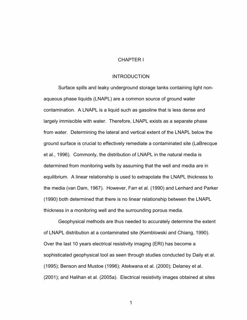
INTRODUCTION
Surface spills and leaky underground storage tanks containing light non-
aqueous phase liquids (LNAPL) are a common source of ground water
contamination. A LNAPL is a liquid such as gasoline that is less dense and
largely immiscible with water. Therefore, LNAPL exists as a separate phase
from water. Determining the lateral and vertical extent of the LNAPL below the
ground surface is crucial to effectively remediate a contaminated site (LaBrecque
et al., 1996). Commonly, the distribution of LNAPL in the natural media is
determined from monitoring wells by assuming that the well and media are in
equilibrium. A linear relationship is used to extrapolate the LNAPL thickness to
the media (van Dam, 1967). However, Farr et al. (1990) and Lenhard and Parker
(1990) both determined that there is no linear relationship between the LNAPL
thickness in a monitoring well and the surrounding porous media.
Geophysical methods are thus needed to accurately determine the extent
of LNAPL distribution at a contaminated site (Kemblowski and Chiang, 1990).
Over the last 10 years electrical resistivity imaging (ERI) has become a
sophisticated geophysical tool as seen through studies conducted by Daily et al.
(1995); Benson and Mustoe (1996); Atekwana et al. (2000); Delaney et al.
(2001); and Halihan et al. (2005a). Electrical resistivity images obtained at sites
1
contaminated with LNAPL often show the distribution of LNAPL affected by the
location of boreholes in either an attractive or repulsive fashion (Halihan et al.,
2005a). This will result in an anomalously low or high estimate of the amount of
LNAPL in the formation using measurements from such wells.
Purpose of Study
This study examined the influence of borehole construction on LNAPL
thickness measurements taken from monitoring wells. A numerical model was
constructed to test the hypothesis that the hydraulic conductivity contrast
between a borehole and natural media has a significant enough effect to create
either a convergent or divergent two-phase flow field around a borehole. Such a
flow field would lead to inaccurate LNAPL measurements in monitoring wells as
compared to formation concentrations. Electrical resistivity images obtained from
three sites contaminated by LNAPLs provide field evidence to test the hypothesis
that the flow field is affected by the hydraulic conductivity contrast between the
formation and the borehole.
Objectives
1. Evaluate the literature for the expected range of hydraulic conductivity
values for borehole construction and natural media.
2. Evaluate the literature for studies conducted on the interaction of two-
phase flow and wells.
2

3. Evaluate the literature for previous studies that apply electrical
resistivity imaging to locate light non-aqueous phase liquids within the
subsurface.
4. Numerically model the two-phase flow (LNAPL and water) interaction
around a borehole within porous media under natural gradient conditions
using COMSOL Multiphysics 3.3a.
5. Compare the model results to field data collected with electrical
resistivity imaging surveys and core samples. Images were taken at three
sites within Oklahoma that are contaminated by LNAPLs from leaky
underground storage tanks.
Field Sites
Electrical resistivity surveys were conducted at three sites in Oklahoma
(Figure 1.1) to identify LNAPLs that had leaked and migrated from underground
storage tanks (UST). The Oklahoma Corporation Commission (OCC) Petroleum
Storage Tank Division invited Oklahoma State University’s (OSU) School of
Geology to investigate the study sites in Golden and Enid, OK. The site in Enid
was evaluated prior to and during remediation, while the site at Golden had
already gone through remediation. Aestus, LLC, an environmental consulting
firm out of Colorado, was contracted by the OCC to examine a commercial site in
Hobart, OK that was in the preliminary site characterization phase.
3
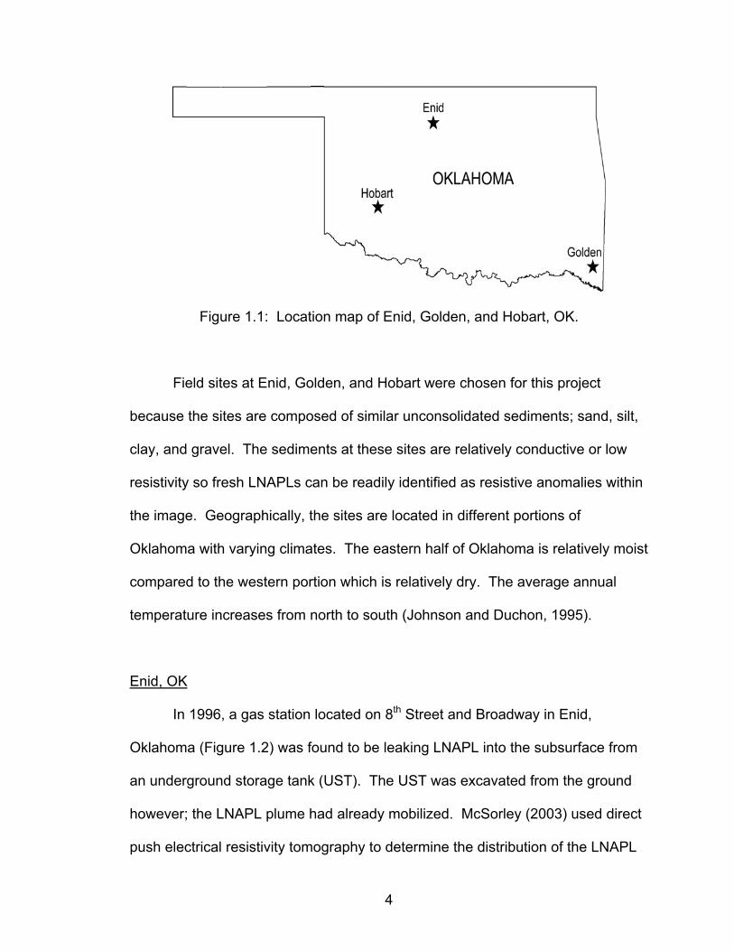
Figure 1.1: Location map of Enid, Golden, and Hobart, OK.
Field sites at Enid, Golden, and Hobart were chosen for this project
because the sites are composed of similar unconsolidated sediments; sand, silt,
clay, and gravel. The sediments at these sites are relatively conductive or low
resistivity so fresh LNAPLs can be readily identified as resistive anomalies within
the image. Geographically, the sites are located in different portions of
Oklahoma with varying climates. The eastern half of Oklahoma is relatively moist
compared to the western portion which is relatively dry. The average annual
temperature increases from north to south (Johnson and Duchon, 1995).
Enid, OK
In 1996, a gas station located on 8th Street and Broadway in Enid,
Oklahoma (Figure 1.2) was found to be leaking LNAPL into the subsurface from
an underground storage tank (UST). The UST was excavated from the ground
however; the LNAPL plume had already mobilized. McSorley (2003) used direct
push electrical resistivity tomography to determine the distribution of the LNAPL
4
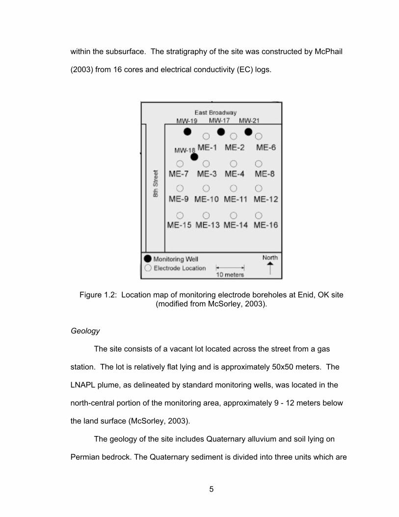
within the subsurface. The stratigraphy of the site was constructed by McPhail
(2003) from 16 cores and electrical conductivity (EC) logs.
Figure 1.2: Location map of monitoring electrode boreholes at Enid, OK site (modified from McSorley, 2003).
Geology
The site consists of a vacant lot located across the street from a gas
station. The lot is relatively flat lying and is approximately 50x50 meters. The
LNAPL plume, as delineated by standard monitoring wells, was located in the
north-central portion of the monitoring area, approximately 9 - 12 meters below
the land surface (McSorley, 2003).
The geology of the site includes Quaternary alluvium and soil lying on
Permian bedrock. The Quaternary sediment is divided into three units which are
5
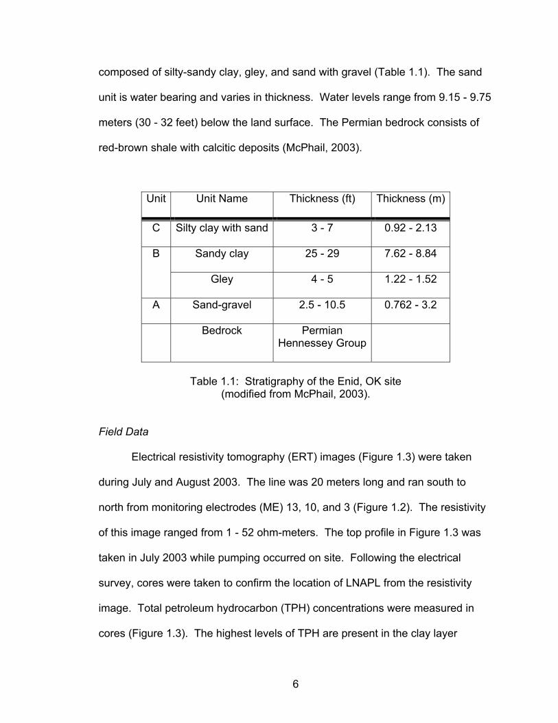
composed of silty-sandy clay, gley, and sand with gravel (Table 1.1). The sand
unit is water bearing and varies in thickness. Water levels range from 9.15 - 9.75
meters (30 - 32 feet) below the land surface. The Permian bedrock consists of
red-brown shale with calcitic deposits (McPhail, 2003).
Unit Unit Name Thickness (ft) Thickness (m)
C Silty clay with sand 3 - 7 0.92 - 2.13
Sandy clay 25 - 29 7.62 - 8.84 B
Gley 4 - 5 1.22 - 1.52
A Sand-gravel 2.5 - 10.5 0.762 - 3.2
Bedrock Permian Hennessey Group
Table 1.1: Stratigraphy of the Enid, OK site
(modified from McPhail, 2003).
Field Data
Electrical resistivity tomography (ERT) images (Figure 1.3) were taken
during July and August 2003. The line was 20 meters long and ran south to
north from monitoring electrodes (ME) 13, 10, and 3 (Figure 1.2). The resistivity
of this image ranged from 1 - 52 ohm-meters. The top profile in Figure 1.3 was
taken in July 2003 while pumping occurred on site. Following the electrical
survey, cores were taken to confirm the location of LNAPL from the resistivity
image. Total petroleum hydrocarbon (TPH) concentrations were measured in
cores (Figure 1.3). The highest levels of TPH are present in the clay layer
6
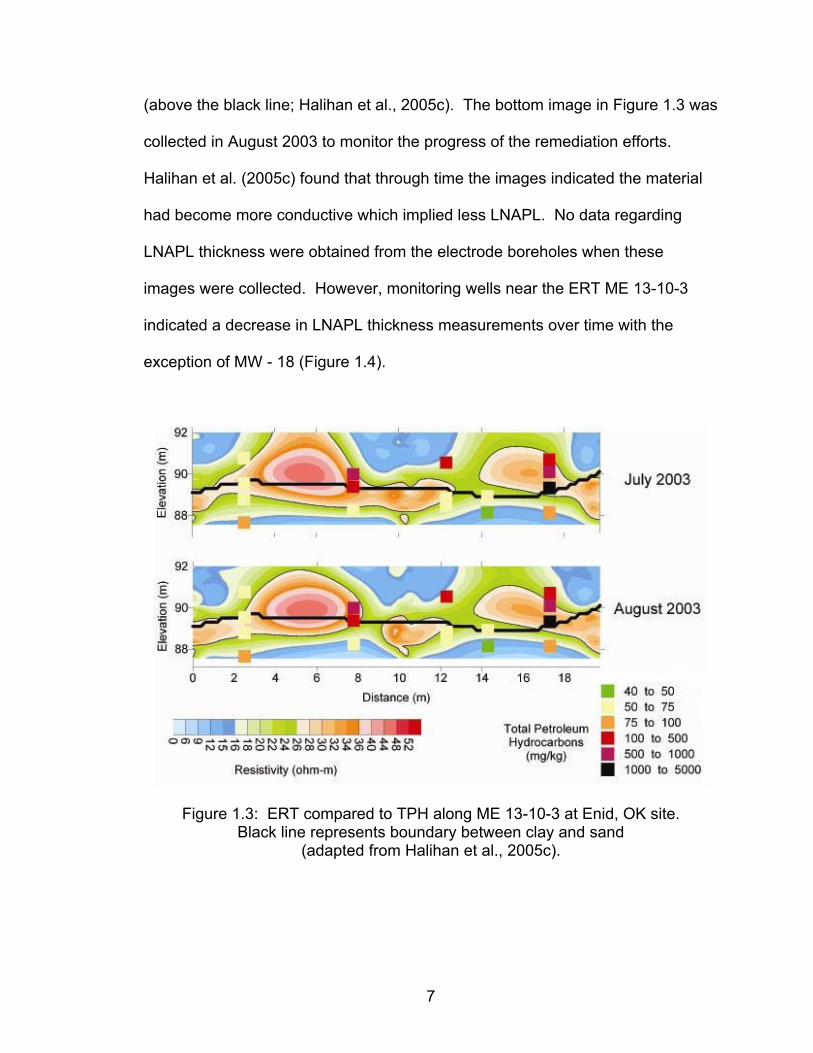
(above the black line; Halihan et al., 2005c). The bottom image in Figure 1.3 was
collected in August 2003 to monitor the progress of the remediation efforts.
Halihan et al. (2005c) found that through time the images indicated the material
had become more conductive which implied less LNAPL. No data regarding
LNAPL thickness were obtained from the electrode boreholes when these
images were collected. However, monitoring wells near the ERT ME 13-10-3
indicated a decrease in LNAPL thickness measurements over time with the
exception of MW - 18 (Figure 1.4).
Figure 1.3: ERT compared to TPH along ME 13-10-3 at Enid, OK site. Black line represents boundary between clay and sand
(adapted from Halihan et al., 2005c).
7
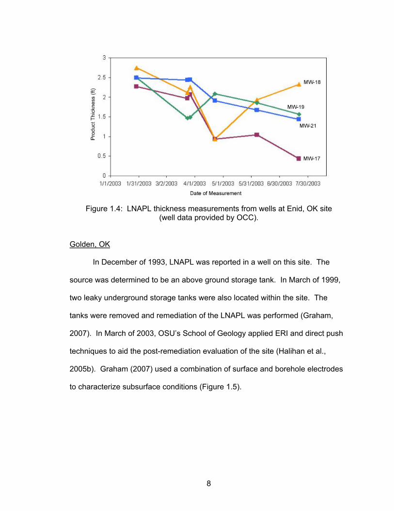
Figure 1.4: LNAPL thickness measurements from wells at Enid, OK site
(well data provided by OCC).
Golden, OK
In December of 1993, LNAPL was reported in a well on this site. The
source was determined to be an above ground storage tank. In March of 1999,
two leaky underground storage tanks were also located within the site. The
tanks were removed and remediation of the LNAPL was performed (Graham,
2007). In March of 2003, OSU’s School of Geology applied ERI and direct push
techniques to aid the post-remediation evaluation of the site (Halihan et al.,
2005b). Graham (2007) used a combination of surface and borehole electrodes
to characterize subsurface conditions (Figure 1.5).
8
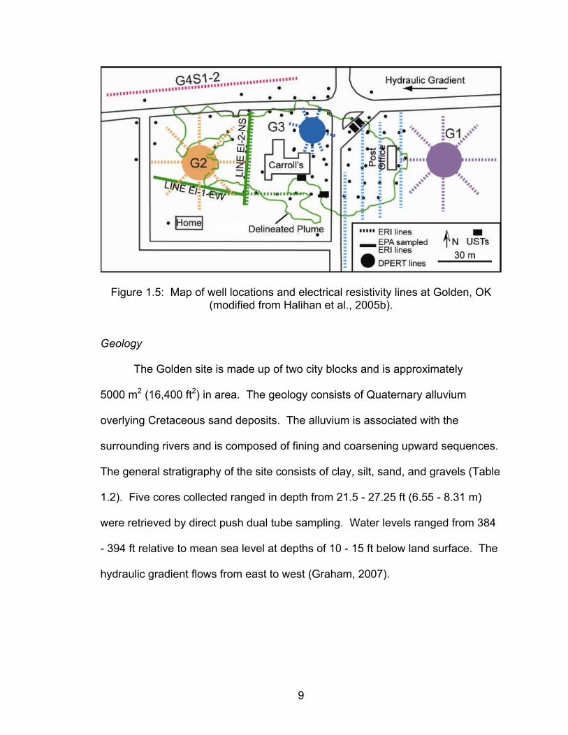
Figure 1.5: Map of well locations and electrical resistivity lines at Golden, OK (modified from Halihan et al., 2005b).
Geology
The Golden site is made up of two city blocks and is approximately
5000 m2 (16,400 ft2) in area. The geology consists of Quaternary alluvium
overlying Cretaceous sand deposits. The alluvium is associated with the
surrounding rivers and is composed of fining and coarsening upward sequences.
The general stratigraphy of the site consists of clay, silt, sand, and gravels (Table
1.2). Five cores collected ranged in depth from 21.5 - 27.25 ft (6.55 - 8.31 m)
were retrieved by direct push dual tube sampling. Water levels ranged from 384
- 394 ft relative to mean sea level at depths of 10 - 15 ft below land surface. The
hydraulic gradient flows from east to west (Graham, 2007).
9
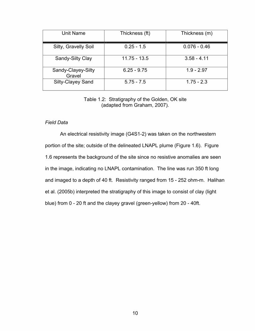
Unit Name Thickness (ft) Thickness (m)
Silty, Gravelly Soil 0.25 - 1.5 0.076 - 0.46
Sandy-Silty Clay 11.75 - 13.5 3.58 - 4.11
Sandy-Clayey-Silty Gravel
6.25 - 9.75 1.9 - 2.97
Silty-Clayey Sand 5.75 - 7.5 1.75 - 2.3
Table 1.2: Stratigraphy of the Golden, OK site
(adapted from Graham, 2007).
Field Data
An electrical resistivity image (G4S1-2) was taken on the northwestern
portion of the site; outside of the delineated LNAPL plume (Figure 1.6). Figure
1.6 represents the background of the site since no resistive anomalies are seen
in the image, indicating no LNAPL contamination. The line was run 350 ft long
and imaged to a depth of 40 ft. Resistivity ranged from 15 - 252 ohm-m. Halihan
et al. (2005b) interpreted the stratigraphy of this image to consist of clay (light
blue) from 0 - 20 ft and the clayey gravel (green-yellow) from 20 - 40ft.
10
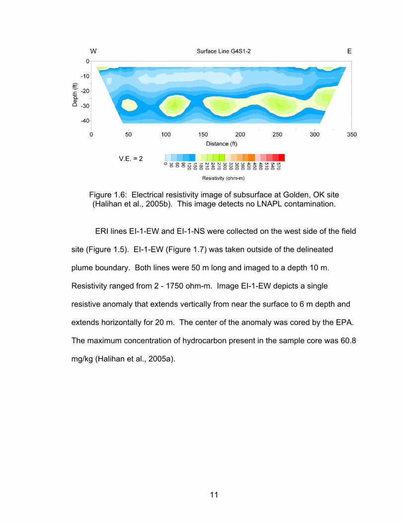
Figure 1.6: Electrical resistivity image of subsurface at Golden, OK site (Halihan et al., 2005b). This image detects no LNAPL contamination.
ERI lines EI-1-EW and EI-1-NS were collected on the west side of the field
site (Figure 1.5). EI-1-EW (Figure 1.7) was taken outside of the delineated
plume boundary. Both lines were 50 m long and imaged to a depth 10 m.
Resistivity ranged from 2 - 1750 ohm-m. Image EI-1-EW depicts a single
resistive anomaly that extends vertically from near the surface to 6 m depth and
extends horizontally for 20 m. The center of the anomaly was cored by the EPA.
The maximum concentration of hydrocarbon present in the sample core was 60.8
mg/kg (Halihan et al., 2005a).
11
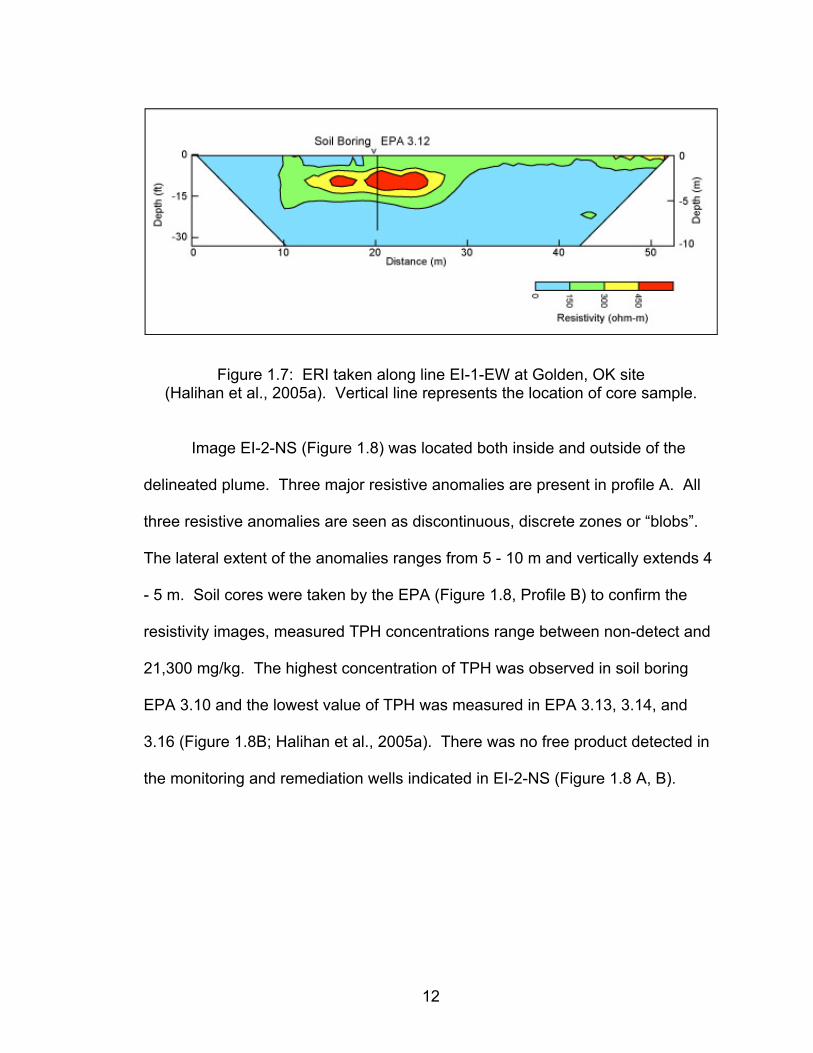
Figure 1.7: ERI taken along line EI-1-EW at Golden, OK site (Halihan et al., 2005a). Vertical line represents the location of core sample.
Image EI-2-NS (Figure 1.8) was located both inside and outside of the
delineated plume. Three major resistive anomalies are present in profile A. All
three resistive anomalies are seen as discontinuous, discrete zones or “blobs”.
The lateral extent of the anomalies ranges from 5 - 10 m and vertically extends 4
- 5 m. Soil cores were taken by the EPA (Figure 1.8, Profile B) to confirm the
resistivity images, measured TPH concentrations range between non-detect and
21,300 mg/kg. The highest concentration of TPH was observed in soil boring
EPA 3.10 and the lowest value of TPH was measured in EPA 3.13, 3.14, and
3.16 (Figure 1.8B; Halihan et al., 2005a). There was no free product detected in
the monitoring and remediation wells indicated in EI-2-NS (Figure 1.8 A, B).
12
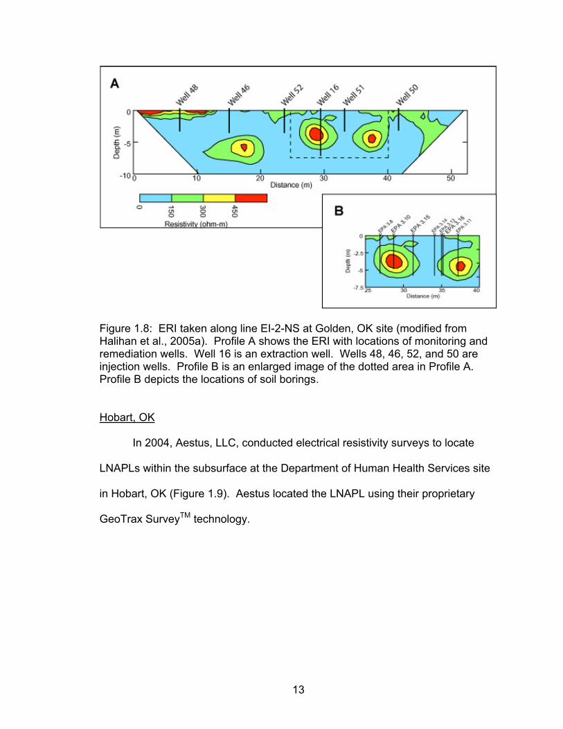
Figure 1.8: ERI taken along line EI-2-NS at Golden, OK site (modified from Halihan et al., 2005a). Profile A shows the ERI with locations of monitoring and remediation wells. Well 16 is an extraction well. Wells 48, 46, 52, and 50 are injection wells. Profile B is an enlarged image of the dotted area in Profile A. Profile B depicts the locations of soil borings.
Hobart, OK
In 2004, Aestus, LLC, conducted electrical resistivity surveys to locate
LNAPLs within the subsurface at the Department of Human Health Services site
in Hobart, OK (Figure 1.9). Aestus located the LNAPL using their proprietary
GeoTrax SurveyTM technology.
13
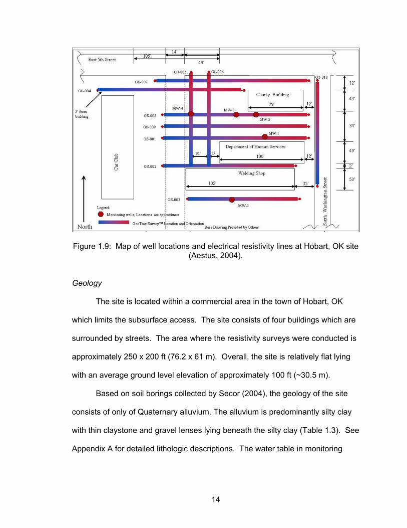
Figure 1.9: Map of well locations and electrical resistivity lines at Hobart, OK site
(Aestus, 2004).
Geology
The site is located within a commercial area in the town of Hobart, OK
which limits the subsurface access. The site consists of four buildings which are
surrounded by streets. The area where the resistivity surveys were conducted is
approximately 250 x 200 ft (76.2 x 61 m). Overall, the site is relatively flat lying
with an average ground level elevation of approximately 100 ft (~30.5 m).
Based on soil borings collected by Secor (2004), the geology of the site
consists of only of Quaternary alluvium. The alluvium is predominantly silty clay
with thin claystone and gravel lenses lying beneath the silty clay (Table 1.3). See
Appendix A for detailed lithologic descriptions. The water table in monitoring
14
wells (MW) 1 - 5 was approximately 12 ft (3.7 m) below the land surface. Ground
water flows from east to west on this site (Figure 1.9).
Unit Name Thickness (ft) Thickness (m)
Silty Clay ~15 ft 4.6 m
Gravel 0.5 - 1.5 ft 0.15 - 0.46 m
Claystone 0.5 - 1 ft 0.15 - 0.3 m
Table 1.3: Stratigraphy of the Hobart, OK site
(adapted from Secor, 2004).
Field Data
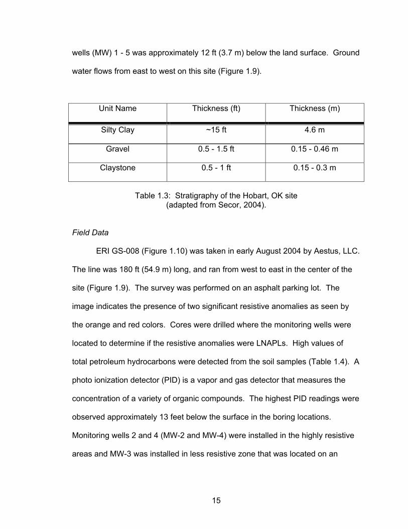
ERI GS-008 (Figure 1.10) was taken in early August 2004 by Aestus, LLC.
The line was 180 ft (54.9 m) long, and ran from west to east in the center of the
site (Figure 1.9). The survey was performed on an asphalt parking lot. The
image indicates the presence of two significant resistive anomalies as seen by
the orange and red colors. Cores were drilled where the monitoring wells were
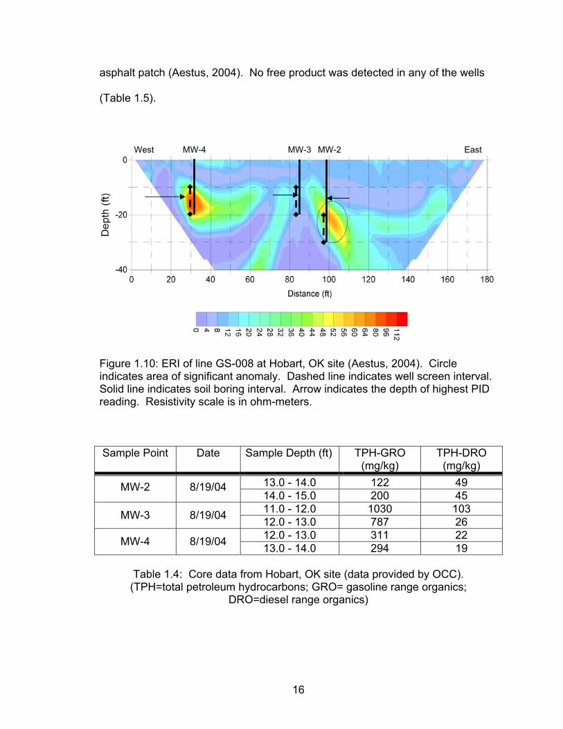
located to determine if the resistive anomalies were LNAPLs. High values of
total petroleum hydrocarbons were detected from the soil samples (Table 1.4). A
photo ionization detector (PID) is a vapor and gas detector that measures the
concentration of a variety of organic compounds. The highest PID readings were
observed approximately 13 feet below the surface in the boring locations.
Monitoring wells 2 and 4 (MW-2 and MW-4) were installed in the highly resistive
areas and MW-3 was installed in less resistive zone that was located on an
15
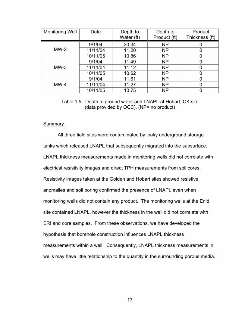
asphalt patch (Aestus, 2004). No free product was detected in any of the wells
(Table 1.5).
West MW-4 MW-3 MW-2 East
Figure 1.10: ERI of line GS-008 at Hobart, OK site (Aestus, 2004). Circle indicates area of significant anomaly. Dashed line indicates well screen interval. Solid line indicates soil boring interval. Arrow indicates the depth of highest PID reading. Resistivity scale is in ohm-meters. Sample Point Date Sample Depth (ft) TPH-GRO
(mg/kg) TPH-DRO
(mg/kg) 13.0 - 14.0 122 49 MW-2 8/19/04 14.0 - 15.0 200 45 11.0 - 12.0 1030 103 MW-3 8/19/04 12.0 - 13.0 787 26 12.0 - 13.0 311 22 MW-4 8/19/04 13.0 - 14.0 294 19
Table 1.4: Core data from Hobart, OK site (data provided by OCC).
(TPH=total petroleum hydrocarbons; GRO= gasoline range organics; DRO=diesel range organics)
16
Monitoring Well Date Depth to Water (ft)
Depth to Product (ft)
Product Thickness (ft)
9/1/04 20.34 NP 0 11/11/04 11.20 NP 0 MW-2 10/11/05 10.86 NP 0 9/1/04 11.49 NP 0
11/11/04 11.12 NP 0 MW-3 10/11/05 10.62 NP 0 9/1/04 11.61 NP 0
11/11/04 11.27 NP 0 MW-4 10/11/05 10.75 NP 0
Table 1.5: Depth to ground water and LNAPL at Hobart, OK site
(data provided by OCC). (NP= no product)
Summary
All three field sites were contaminated by leaky underground storage
tanks which released LNAPL that subsequently migrated into the subsurface.
LNAPL thickness measurements made in monitoring wells did not correlate with
electrical resistivity images and direct TPH measurements from soil cores.
Resistivity images taken at the Golden and Hobart sites showed resistive
anomalies and soil boring confirmed the presence of LNAPL even when
monitoring wells did not contain any product. The monitoring wells at the Enid
site contained LNAPL, however the thickness in the well did not correlate with
ERI and core samples. From these observations, we have developed the
hypothesis that borehole construction influences LNAPL thickness
measurements within a well. Consequently, LNAPL thickness measurements in
wells may have little relationship to the quantity in the surrounding porous media.
17
CHAPTER II
REVIEW OF LITERATURE
A numerical model is constructed in this study to examine the influence of
borehole construction on LNAPL thickness measurements. Therefore, a general
description of borehole construction will be provided for both monitoring and
pumping wells. Significant parameters and variables of the natural media and
borehole construction will be explained. The basic theory of hydraulic
conductivity as well as the known values for natural media and borehole
construction materials will also be presented. These values will subsequently be
used in the numerical model.
Previous efforts to model the volume estimation of hydrocarbon within
porous media from fluid levels within a well will be reviewed. Studies performed
to delineate LNAPL contamination within the subsurface through the use of
electrical resistivity surveys will also be discussed. Finally, a previous study
using COMSOL Multiphysics to model two-phase flow is described.
Borehole Construction
Monitoring Wells
Monitoring wells (Figure 2.1) are used to record head measurements in
saturated media, sample ground water, and numerous other tests. Water flows
18
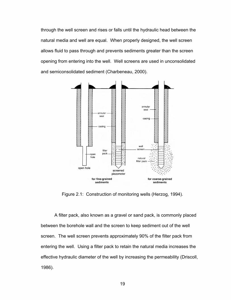
through the well screen and rises or falls until the hydraulic head between the
natural media and well are equal. When properly designed, the well screen
allows fluid to pass through and prevents sediments greater than the screen
opening from entering into the well. Well screens are used in unconsolidated
and semiconsolidated sediment (Charbeneau, 2000).
Figure 2.1: Construction of monitoring wells (Herzog, 1994).
A filter pack, also known as a gravel or sand pack, is commonly placed
between the borehole wall and the screen to keep sediment out of the well
screen. The well screen prevents approximately 90% of the filter pack from
entering the well. Using a filter pack to retain the natural media increases the
effective hydraulic diameter of the well by increasing the permeability (Driscoll,
1986).
19
An annular seal, typically consisting of bentonite, is placed between the
well casing and borehole wall above the screened interval. The seal obstructs
down hole movement of sediment and fluids within the natural media. The seal
is poured or pumped onto the top of the filter pack material to isolate the zone
from which the well is sampling (Weight and Sonderegger, 2001).
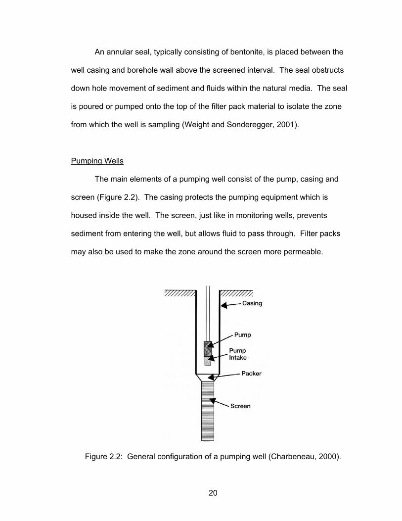
Pumping Wells
The main elements of a pumping well consist of the pump, casing and
screen (Figure 2.2). The casing protects the pumping equipment which is
housed inside the well. The screen, just like in monitoring wells, prevents
sediment from entering the well, but allows fluid to pass through. Filter packs
may also be used to make the zone around the screen more permeable.
Figure 2.2: General configuration of a pumping well (Charbeneau, 2000).
20
Significant Parameters and Variables
Several significant parameters and variables must be considered to define
flow within a two-phase system. These variables will be used in the numerical
model generated for this study. The hydraulic conductivity values for natural
media and borehole construction are presented first since all of the subsequent
variables are allocated by this value.
Hydraulic Conductivity
Hydraulic conductivity as defined by Fetter (2001) is the coefficient of
proportionality describing the rate at which water can be transmitted through
porous media. This can be written mathematically as:
)/( dLdhAQK −
= (2.1)
where K is the hydraulic conductivity (L/T); Q is discharge (L3/T); A is the cross-
sectional area (L2); and dh/dL is the gradient (L/L). Hydraulic conductivity also
depends on the density and viscosity of the fluids flowing through the natural
media (although when not defined, one generally assumes the fluid is water):
μρ gkK = (2.2)
where k is the intrinsic permeability (L2); ρ is the density of the fluid (M/L3); g is
gravitational acceleration (L/T2); and μ is the dynamic viscosity (M/LT); (de
Marsily, 1986). Intrinsic permeability is a function of only the natural media,
therefore an aquifer will have different hydraulic conductivities for water and
LNAPL but the aquifer has the same intrinsic permeability for both fluids. Typical
21
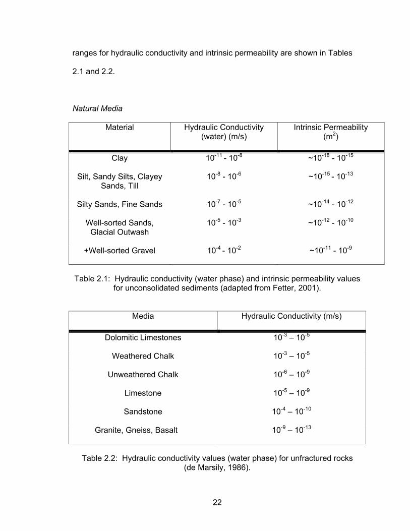
ranges for hydraulic conductivity and intrinsic permeability are shown in Tables
2.1 and 2.2.
Natural Media
Material Hydraulic Conductivity (water) (m/s)
Intrinsic Permeability (m2)
Clay 10-11 - 10-8 ~10-18 - 10-15
Silt, Sandy Silts, Clayey Sands, Till
10-8 - 10-6 ~10-15 - 10-13
Silty Sands, Fine Sands 10-7 - 10-5 ~10-14 - 10-12
Well-sorted Sands, Glacial Outwash
10-5 - 10-3 ~10-12 - 10-10
+Well-sorted Gravel 10-4 - 10-2 ~10-11 - 10-9
Table 2.1: Hydraulic conductivity (water phase) and intrinsic permeability values
for unconsolidated sediments (adapted from Fetter, 2001).
Media Hydraulic Conductivity (m/s)
Dolomitic Limestones 10-3 – 10-5
Weathered Chalk 10-3 – 10-5
Unweathered Chalk 10-6 – 10-9
Limestone 10-5 – 10-9
Sandstone 10-4 – 10-10
Granite, Gneiss, Basalt 10-9 – 10-13
Table 2.2: Hydraulic conductivity values (water phase) for unfractured rocks
(de Marsily, 1986).
22
Borehole Construction
The hydraulic conductivity values for borehole construction were based on
the filter pack and annular seal. The fact that the inside of a borehole is an
empty space was also considered. These values were used in the numerical
model constructed in this study to determine the influence of borehole
construction on two-phase flow.
Filter Pack
Filter pack material should consist of clean, well rounded, homogeneous
sand or gravel. Using this type of material increases the permeability and
porosity of the filter pack. Filter packs are beneficial in highly uniform, fine
grained or highly laminated sediments (Driscoll, 1986). The hydraulic
conductivity, K, of a filter pack is estimated using Equation 2.2. Driscoll (1986)
determined upper limit for the hydraulic conductivity of filter pack material to be
17,000 gpd/ft2 (8.02x10⁻³ m/s).
Annular Seal
An annular seal typically consists of bentonite chips or pellets. Bentonite
is composed of smectite minerals which have a low hydraulic conductivity to
water, large cation exchange capacity, high swelling potential, and large surface
area. The most common bentonite is calcium and sodium bentonite. At a
confining stress of 35 kPa, the hydraulic conductivity of calcium bentonite is
23
6x10-11 m/s and sodium bentonite is 6x10-12 m/s, relative to tap water (Gleason,
et al., 1997).
Capillary Pressure and Fluid Saturation
Capillary pressure and saturation of two fluid phases (water and LNAPL)
are based on the pore size distribution within the natural media. Capillary
pressure is defined as the pressure difference between the non-wetting (LNAPL)
and wetting (water) phases in porous media (Charbeneau, 2000). Fluid
saturation equals the volume of a fluid divided by the volume of void space.
Within a two-phase system the void space within the porous media is assumed to
be completely filled with LNAPL and/or water, therefore the fluid saturation of
either phase can range from 0 to 1 (Charbeneau et al., 1999).
van Genuchten Model Parameters
The relationship between capillary pressure and saturation is determined
by using soil moisture characteristic curves (Figure 2.3). Data for capillary
pressure and water content are often measured in laboratory experiments and
then fit with mathematical models to produce smooth curves.
24
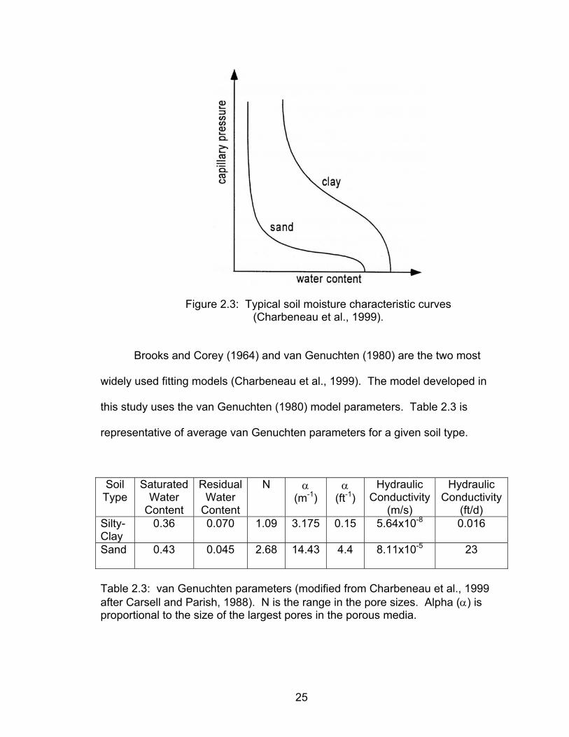
Figure 2.3: Typical soil moisture characteristic curves (Charbeneau et al., 1999).
Brooks and Corey (1964) and van Genuchten (1980) are the two most
widely used fitting models (Charbeneau et al., 1999). The model developed in
this study uses the van Genuchten (1980) model parameters. Table 2.3 is
representative of average van Genuchten parameters for a given soil type.
Soil Type
Saturated Water
Content
ResidualWater
Content
N α (m-1)
α (ft-1)
Hydraulic Conductivity
(m/s)
Hydraulic Conductivity
(ft/d) Silty- Clay
0.36 0.070 1.09 3.175 0.15 5.64x10⁻⁸ 0.016
Sand 0.43 0.045 2.68 14.43 4.4 8.11x10⁻⁵ 23
Table 2.3: van Genuchten parameters (modified from Charbeneau et al., 1999 after Carsell and Parish, 1988). N is the range in the pore sizes. Alpha (α) is proportional to the size of the largest pores in the porous media.
25
Two-phase Flow and Wells
To the author’s knowledge, no previous modeling efforts have been used
to determine the type of flow field that is created around a borehole based on the
hydraulic conductivity contrast between the borehole and surrounding natural
media in a two-phase oil/water system. However, several studies have been
conducted to examine the relationship between fluid levels measured in wells
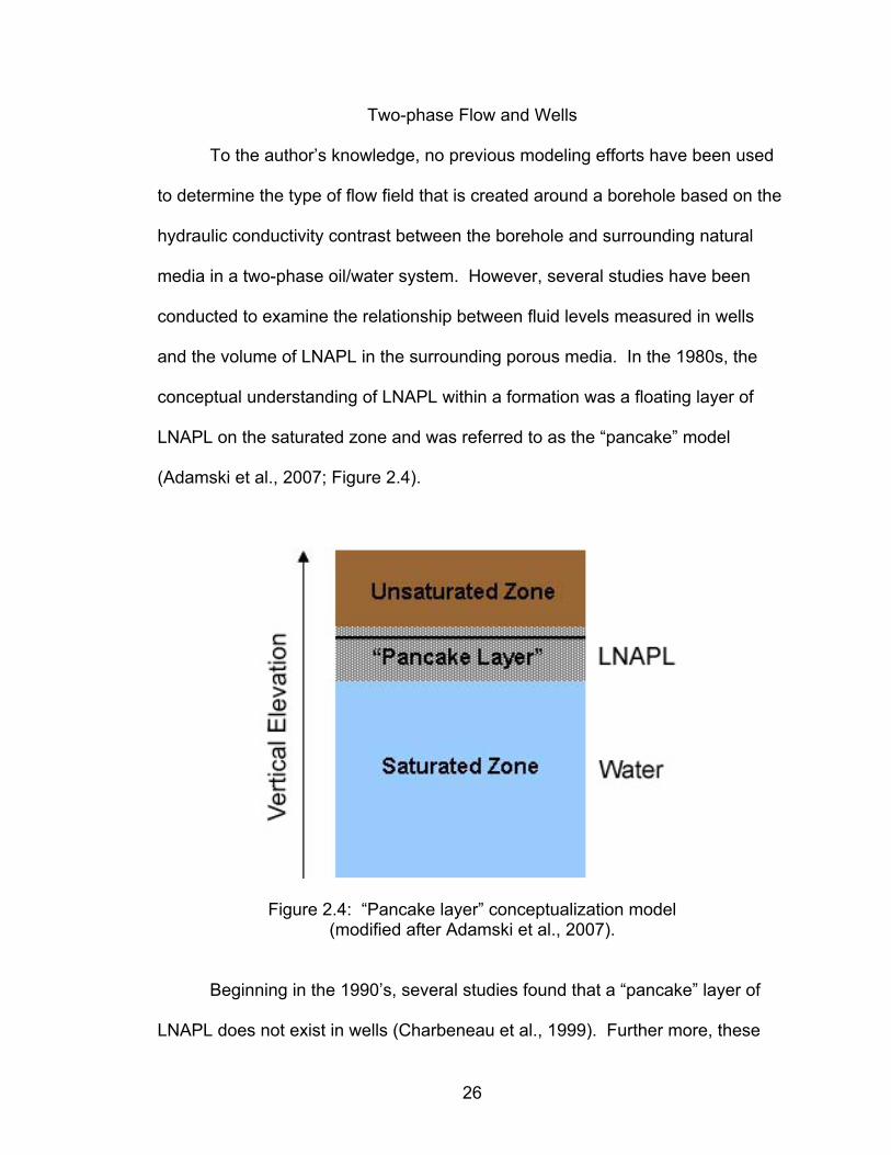
and the volume of LNAPL in the surrounding porous media. In the 1980s, the
conceptual understanding of LNAPL within a formation was a floating layer of
LNAPL on the saturated zone and was referred to as the “pancake” model
(Adamski et al., 2007; Figure 2.4).
Figure 2.4: “Pancake layer” conceptualization model (modified after Adamski et al., 2007).
Beginning in the 1990’s, several studies found that a “pancake” layer of
LNAPL does not exist in wells (Charbeneau et al., 1999). Further more, these
26
studies also showed that the relationship between a well and the surrounding
media is more complex than a simple linear correlation. Factors affecting the
measurement of LNAPL thickness in a formation include multiphase interaction in
the well (Kembloski and Chiang, 1990; Ballestero et al., 1994; Sleep et al., 2000),
capillary pressure (Farr et al., 1990; Lenhard and Parker, 1990; Vogler et al.,
2001; Aral and Liao, 2002; Huntley et al., 1994a), ground water table fluctuations
(Ballestero et al., 1994; Liao and Aral, 1999; Vogler et al., 2001; Aral and Liao,
2002), sediment variability (Wallace and Huntley, 1992; Huntley et al., 1994;
Ballestero et al., 1994; Adamski et al., 2005) and sediment pore size (Lenhard
and Parker, 1990) in the aquifer.
All of the studies developed either numerical, analytical, or conceptual
models based on theoretical, experimental, and field data. Most of the models
assume homogenous media and mechanical equilibrium between the well and
formation. However, Sleep et al. (2000) found that mechanical equilibrium and
homogenous media can not be assumed for accurate volume estimations of the
LNAPL. In order for equilibrium conditions to be achieved between a well and
the formation, the vertical pressure distributions of the two-phases (water and
LNAPL) must be hydrostatic (Figure 2.5; Charbeneau, 2000). Hydrostatic
conditions imply there is no lateral or vertical movement of the fluid and the
pressure gradient results from the vertical attribute of the overlying fluids
(Dahlberg, 1995).
27
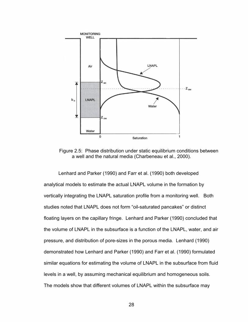
Figure 2.5: Phase distribution under static equilibrium conditions between a well and the natural media (Charbeneau et al., 2000).
Lenhard and Parker (1990) and Farr et al. (1990) both developed
analytical models to estimate the actual LNAPL volume in the formation by
vertically integrating the LNAPL saturation profile from a monitoring well. Both
studies noted that LNAPL does not form “oil-saturated pancakes” or distinct
floating layers on the capillary fringe. Lenhard and Parker (1990) concluded that
the volume of LNAPL in the subsurface is a function of the LNAPL, water, and air
pressure, and distribution of pore-sizes in the porous media. Lenhard (1990)
demonstrated how Lenhard and Parker (1990) and Farr et al. (1990) formulated
similar equations for estimating the volume of LNAPL in the subsurface from fluid
levels in a well, by assuming mechanical equilibrium and homogeneous soils.
The models show that different volumes of LNAPL within the subsurface may
28
produce the same thickness of LNAPL within the monitoring well. The authors
concluded that a linear relationship does not exist between the thickness of
LNAPL in a monitoring well and the surrounding porous media. Farr et al. (1990)
also found that the volume of LNAPL in a formation is highly dependent upon
capillary properties of the porous media.
Kembloski and Chiang (1990) examined factors that control fluctuations in
hydrocarbon thicknesses measured in monitoring wells. Both equilibrium and
non-equilibrium conditions were analyzed and compared to field data.
Equilibrium conditions assume that the vertical pressure head gradient is
negligible and the net flow of fluids is zero between the well and surrounding
porous media. A negative correlation was observed between the measured
hydrocarbon thickness and the change of hydrocarbon/water interface elevation
under non-equilibrium conditions. This inverse relationship was produced by
preferred flow around monitoring wells in conjunction with differing residual
hydrocarbon saturations above and below the hydrocarbon/water interface. The
authors concluded that the hydrocarbon thickness in porous media can not be
determined from monitoring wells. A geophysical approach was recommended
to estimate the oil distribution in a formation.
Ballestero et al. (1994) related the apparent thickness of LNAPL in a
monitoring well to the actual LNAPL thickness in the formation. The authors
found that the main factors in determining the actual LNAPL thickness include
apparent product thickness in the well, product density, water table fluctuations,
29
and grain size distribution in the aquifer. The authors formulated an equation to
predict the thickness of gasoline in a uniform sand aquifer as follows:
agg hStt −−= )1( (2.3)
where tg is the actual hydrocarbon thickness, t is the apparent thickness, Sg is the
specific gravity of the hydrocarbon, and ha is the distance between hydrocarbon
and the water table. Note that water table fluctuations were not considered in
this equation.
Huntley et al. (1994b) investigated the influence of sediment variability on
volume estimations of hydrocarbons. The study was conducted at two sites with
relatively homogenous fine grained sandstone aquifers. A similar study was
conducted by Wallace and Huntley (1992). Soil saturation/ capillary pressure
characteristic curves were plotted from aquifer grain size data. Both studies
found that a single “average” soil sample is not representative of an aquifer and
can not be used to calculate the actual amount of hydrocarbon, even on small
sites. Grain-size distribution data was even found to produce errors in the
volume estimation of hydrocarbon. Both papers concluded that the apparent
hydrocarbon thickness measured in a monitoring well should be corrected with
soil saturation/capillary pressure characteristic curves to more accurately
estimate the hydrocarbon volume. Hydrocarbon volumes were calculated using
the Van Genuchten fitting parameters (α, n, and residual saturation) and the
corresponding curve.
Beckett and Huntley (1998) used a three dimensional, finite-element
model, MAGNAS3 to study the effect of soil type on LNAPL recovery rates.
30
Three different soil types were modeled with air, water, and LNAPL phases
included. Several recovery designs were simulated to determine which was most
effective for each soil. The authors noted that hydrocarbon saturation and
movement within the subsurface was dependent on fluid properties, soil
capillarity, and permeability. The study concluded that recovery efforts in any
type of soil decreased the permeability around the well which decreased the
LNAPL saturation and mobility into the well.
Liao and Aral (1999) used two analytical models to examine the effect of
unsteady ground water fluctuations on the amount of LNAPL in a monitoring well.
The models simulated an unconfined aquifer with rising and falling piezometric
head conditions. Residual saturation of the LNAPL was assumed to be constant.
The models indicated that ground water fluctuation has a significant effect on
LNAPL measurements which would cause error in volume calculations of LNAPL
in the porous media. The authors concluded that their models represented a
method to estimate hydraulic equilibrium conditions at contaminated sites.
Sleep et al. (2000) developed a numerical model to determine LNAPL
thickness in finite volume monitoring wells. The model incorporated gravity
segregation of water, air, and LNAPL for multiphase flow. A pilot scale
experiment which consisted of layered sandy soil and toluene injection was
conducted to test the validity of the model. Results from the experiment and
model indicated mechanical equilibrium and soil homogeneity could not be
assumed in order to accurately determine the volume of LNAPL within the soil.
31
Vogler et al. (2001) developed an empirical method to estimate the
volume of hydrocarbon contamination within the subsurface from fluid levels in
monitoring wells. This method calculated the LNAPL volume by using the oil-air,
water-air, and oil-water capillary pressure and saturation relationships. The
authors noted that the capillary properties of porous media significantly impact
multiphase flow. A laboratory experiment and field investigation was conducted
to study the influence of ground water table fluctuations on flow. The authors
concluded that in order to determine the actual volume of LNAPL contamination
their method and ground water table fluctuations must be considered.
Aral and Liao (2002) used a numerical model to investigate the impact of
water table and capillary pressure fluctuations on LNAPL thickness in monitoring
wells. The authors found that under transient conditions, LNAPL thickness in
the monitoring well were not reflective of the total volume of contamination in the
formation. Capillary pressure at the LNAPL/air and water/LNAPL interfaces
significantly affected the thickness of LNAPL in the monitoring well.
Adamski et al. (2005) developed a conceptual model for LNAPL behavior
in fine grained soil. The authors found that in fine grained soils, macropores
controlled the distribution of LNAPL in the formation. They also concluded that
LNAPL saturation in fine grained soil could be predicted by using the
Charbeneau/API model (Charbeneau et al., 1999), site hydrogeology, soil
sampling, and saturation properties of the soil.
A linear relationship does not exist between the porous media and LNAPL
thickness within a well. Many studies have concluded that mechanical
32
equilibrium between the well and media can not be assumed due to temporal
fluctuations in the water table and capillary pressures; sediment and pore size
variability; and multiphase interaction in the well. For these reasons monitoring
wells should not be utilized as the only tool at sites contaminated by LNAPL to
determine the extent of contamination within the subsurface. Additionally, a well
which does not present detectable levels of hydrocarbon should not be used to
determine if a LNAPL contaminated site is “clean”.
Electrical Resistivity Imaging
Electrical resistivity imaging has progressively become a useful and
sophisticated method to map the extent of LNAPL contamination (Halihan et al.,
2005a). Electrical resistivity measurements are collected through a series of
electrodes which emit current into the subsurface. The potential field is recorded
and the data is inverted to create a map of subsurface resistivity distributions.
ERI is the general term used to describe an array of electrodes on the surface,
without naming each electrode configuration. In contrast, electrical resistivity
tomography (ERT) indicates the electrodes are in the subsurface measuring the
electrical conductivity of the ground (Halihan et al. 2005c).
Daily et al. (1995) conducted three controlled experiments to assess the
accuracy of ERT for the characterization and monitoring of hydrocarbon
contaminated sites. The experiments were performed in a tank which was 10 m2
and 5 m deep. The experiments included a gasoline spill into a sandy soil, air
sparging in a saturated soil, and a leaky oil storage tank. All of the experiments
33
produced resistive anomalies in the ERT images in both saturated and
unsaturated sediment. LNAPL was confirmed through coring to be in the location
of the resistive anomalies.
Benson and Mustoe (1996) determined the extent of hydrocarbon
contamination from a leaky underground storage tank using electrical resistivity
and ground penetrating radar (GPR). GPR data and isoresistivity maps
constructed from the resistivity surveys were used to select locations for
monitoring wells. The authors concluded that geophysical surveys are a cost
effective method to collect data and reduces the risk of blind drilling into
hazardous waste materials.
Loh et al. (1999) investigated the use of ERT to calculate volumetric flow
rates of conductive liquids in nonconductive solids. The authors compared flow
rates derived from ERT to those derived from more traditional methods such as
weighing hoppers, gradiomanometers, and intrusive conductivity probes. There
was a good correlation between the results, indicating that ERT can be used to
determine flow rates.
Atekwana et al. (2000) employed multiple geoelectrical methods and soil
borings to analyze a 50-year-old hydrocarbon contaminated site. Geoelectrical
methods included ground penetrating radar (GPR), electrical resistivity (both
surface and downhole), and electromagnetic induction. The objective was to
determine if the temporal variation in the electrical signal of the LNAPL from
resistive to conductive. The authors found that the electrical signal of the
hydrocarbon did change and hypothesized that this was a result of LNAPL
34
biodegradation. Therefore, the assumption that LNAPL always produces regions
of high resistivity above the water table in geophysical images is not always
correct, due to the evolving nature of the plume. The authors concluded that
surface and downhole geoelectrical measurements at LNAPL contaminated sites
allow for a better site characterization as compared to using only monitoring wells
to delineate LNAPL within the subsurface.
Delaney et al. (2001) examined the change in resistivity of fine-grained
soils at a petroleum contaminated site with both laboratory and field
investigations. The authors noted that electrical resistivity values for clean soils
range from 100 to 10,000 ohm-meters, while unsaturated coarse grained and
frozen soils typically exceed 10,000 ohm-meters. The field survey and laboratory
experiments showed that a soil will have a permanent increase in resistivity due
to residual hydrocarbon contamination. The authors concluded that at petroleum
contaminated sites resistivity values are site dependent.
Kemna et al. (2002) used ERT to image a field tracer (NaBr) experiment in
a heterogeneous unconfined aquifer. The authors noted that it is difficult for
monitoring wells to depict the complex position and shape of a plume. ERT
images taken during the experiment were converted to solute concentration
maps and depicted the spreading of the plume over time. The authors found this
method to be more valuable than using monitoring wells since it allows for the
determination of the center of the plume and has better resolution.
Halihan et al. (2005a) applied ERI to locate remaining hydrocarbons in an
already remediated site. ERI images detected “blobs” of hydrocarbons remaining
35
inside and outside of the remediated area. Hydrocarbons were also detected in
between “clean” monitoring wells. The images were confirmed with drilling. The
authors concluded that ERI is a more efficient and cost effective method to locate
hydrocarbon contamination than installing numerous monitoring wells at the site.
COMSOL Multiphysics
This finite element modeling program allows for the simulation of any
physical phenomenon that can be expressed as a set of partial differential
equations. The program is capable of using multiple equations in a single model.
Grechka and Soutter (2005) used COMSOL to model two-phase flow (oil and
water) fully coupled to the deformation that occurs during fluid production and
injection within a porous reservoir. The model was governed by the equations
established by Brooks and Corey (1966), van Genuchten (1980), and Thurston
(1974). This simulation incorporated changes in pressure, saturation, flow
velocity, and permeability for both oil and water phases.
36
CHAPTER III
METHODOLOGY
A numerical model was developed to determine the influence of borehole
construction on LNAPL thickness measurements. This was be done by modeling
the hydraulic conductivity contrast between the borehole and media to determine
if the two-phase (water and LNAPL) flow field around a borehole is significantly
affected. This chapter presents the two-phase flow numerical simulation by first
defining the model geometry, then establishing the governing equations and
constitutive relationships that define fluid retention and permeability in the natural
media. The formulation of boundary conditions and initial conditions follows.
Numerical Model Development
The two-phase flow numerical simulation was constructed using COMSOL
Multiphysics 3.3a. The numerical model was created in the Earth Science
Module. This module allowed for the simulation of numerous geophysical and
environmental scenarios.
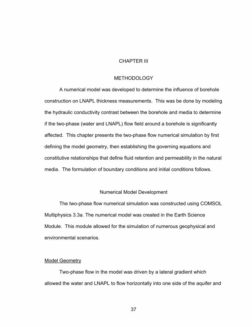
Model Geometry
Two-phase flow in the model was driven by a lateral gradient which
allowed the water and LNAPL to flow horizontally into one side of the aquifer and
37
out the other (Figure 3.1). The dimensions of the aquifer were 50x50 m, with a
borehole in the center. The radius of the borehole was varied in certain
simulations to examine the influence of borehole size on the two-phase flow field.
Figure 3.1: Model geometry in plan view. Scale is in meters.
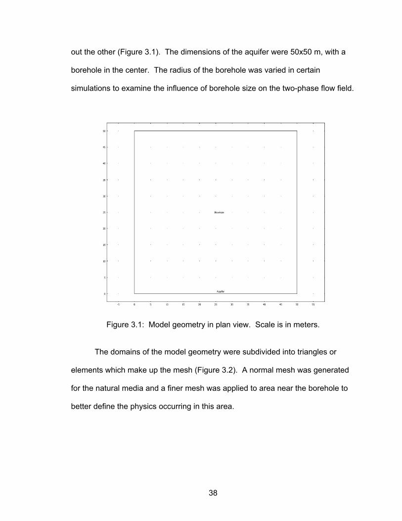
The domains of the model geometry were subdivided into triangles or
elements which make up the mesh (Figure 3.2). A normal mesh was generated
for the natural media and a finer mesh was applied to area near the borehole to
better define the physics occurring in this area.
38
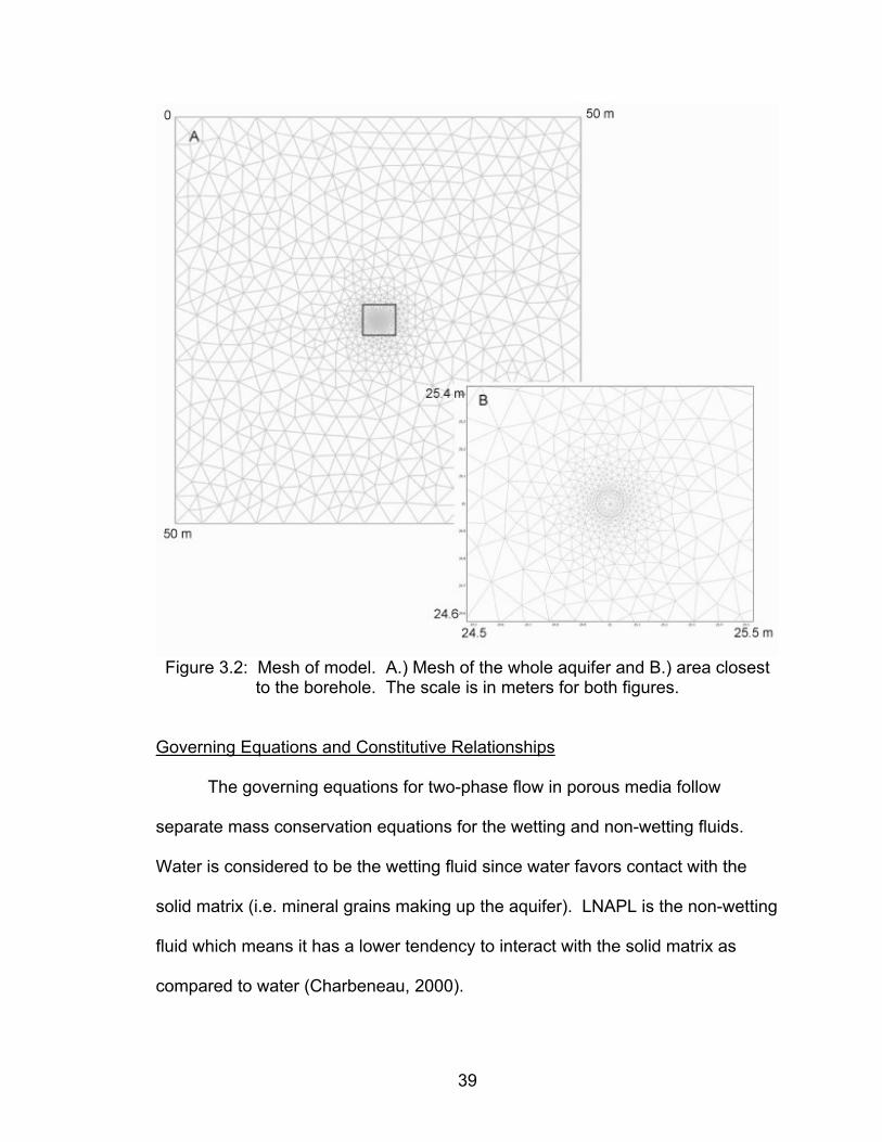
Figure 3.2: Mesh of model. A.) Mesh of the whole aquifer and B.) area closest
to the borehole. The scale is in meters for both figures.
Governing Equations and Constitutive Relationships
The governing equations for two-phase flow in porous media follow
separate mass conservation equations for the wetting and non-wetting fluids.
Water is considered to be the wetting fluid since water favors contact with the
solid matrix (i.e. mineral grains making up the aquifer). LNAPL is the non-wetting
fluid which means it has a lower tendency to interact with the solid matrix as
compared to water (Charbeneau, 2000).
39
The governing equations for multiphase flow are coupled, nonlinear partial
differential equations (PDEs). Constitutive relationships are also integrated into
the PDEs to account for fluid retention and aquifer permeability. The governing
equations and constitutive relationships were taken from a two-phase flow
example in the COMSOL Multiphysics Earth Science Module (2005). The
following equations are based on Mualem (1976) and van Genuchten (1980).
The mass conservation equations for the wetting (w) and non-wetting (nw)
fluids, assuming they are incompressible, are:
( ) 0,int =⎥⎦
⎤⎢⎣
⎡+∇−⋅∇+
∂∂
gDpk
tSe
www
wrws ρ
ηκ
θ (3.1)
( 0,int =⎥⎦
⎤⎢⎣
⎡+∇−⋅∇+
∂∂
gDpk
tSe
nwnwnw
nwrnws ρ
ηκ
θ ) . (3.2)
See the List of Symbols section for nomenclature descriptions. Equations 3.1
and 3.2 are subject to the constraint:
Sew + Senw = 1. (3.3)
This constraint assumes that the void space of the porous media is completely
filled by water and/or LNAPL. The saturation of either fluid phase can range
from 0 to 1.
Capillary pressure is the pressure difference between the non-wetting and
wetting phase interfaces and is mathematically defined as:
pc = pnw - pw. (3.4)
40
Capillary pressure results from the density difference between two fluids and is a
function of the fluid phase saturations. Effective saturation changes with capillary
pressure. This relationship is quantified as:
c
wnwpwp p
SeCC∂∂
=−= s,, θ (3.5)
where Cp is the specific capacity of the wetting and non-wetting phases at a
given pressure.
To numerically simplify the model, Equations 3.3, 3.4, and 3.5 are
substituted in Equations 3.1 and 3.2, so that the governing equations become:
( ) ( ) 0,int, =⎥
⎦
⎤⎢⎣
⎡+∇−⋅∇+−
∂∂ gDp
kpp
tC ww
w
wrwnwwp ρ
ηκ
(3.6)
( ) ( ) 0,int, =⎥
⎦
⎤⎢⎣
⎡+∇−⋅∇+−
∂∂
− gDpk
ppt
C nwnwnw
nwrwnwwp ρ
ηκ
. (3.7)
Fluid Retention and Permeability
The van Genuchten (1980) and Mualem (1976) equations are dependent
on capillary pressure head (Hc) to express fluid retention and permeability for
two-phase flow. The following relationships define how θ, Se, C, kr, and pc vary
simultaneously by transforming capillary pressure to capillary pressure head
which is defined as:
gp
Hw
cc ρ= . (3.8)
41
The hydraulic properties of the wetting fluid phase are given by Equations
3.9-3.12, with the variables defined in the List of Symbols:
⎪⎩
⎪⎨
⎧ −+=
ws
wrwswwr
w
Se
,
,,, )(
θ
θθθθ (3.9)
0
0
≤
>
c
c
H
H
[ ]
⎪⎪⎪
⎩
⎪⎪⎪
⎨
⎧+
=1
11
mnc
w
HSe
α (3.10)
0
0
≤
>
c
c
H
H
⎪⎪⎪
⎩
⎪⎪⎪
⎨
⎧⎟⎠⎞
⎜⎝⎛ −⎟
⎠⎞
⎜⎝⎛ −−
=0
11
11
,,
m
mwmwwrws
w
SeSemm
C
θθα
(3.11) 0
0
≤
>
c
c
H
H
⎪⎪⎪
⎩
⎪⎪⎪
⎨
⎧
⎥⎥⎦
⎤
⎢⎢⎣
⎡⎟⎠⎞
⎜⎝⎛ −−
=1
112
1
,
m
mwL
w
wr
SeSe
k (3.12) 0
0
≤
>
c
c
H
H
42
The hydraulic properties of the non-wetting fluid are given by
Equations 3.13-3.16:
wwsnw θθθ −= , (3.13)
wnw SeSe −= 1 (3.14)
wnw CC −= (3.15)
( )2
1
, 11m
mwL
wnwr SeSek ⎟⎠⎞
⎜⎝⎛ −−= (3.16)
Boundary and Initial Conditions
The boundary conditions in the model for both phases were either
hydrostatic or no-flow. These conditions simulated a confined aquifer and only
allowed the water and LNAPL to flow laterally from one side to the other (Figure
3.3).
43
Figure 3.3: Boundary conditions for the model aquifer shown in plan view. Scale is in meters.
The boundary condition and initial conditions were expressed in terms of
pressure:
hgp ρ= . (3.17)
For the wetting phase, the boundary condition on the right side of the
aquifer was set at 509 Pascals (1 Pa= 1 kg/ms2) and the left is 18 Pa. Initial
conditions for the wetting phase were set as:
1882.9)( += xwp . (3.18)
This equated to a hydraulic gradient of 0.001 m/m, where x was the distance
along the aquifer which was 50 m long, approximating an ambient gradient an
aquifer.
The boundary condition for the non-wetting phase on the right side was a
function of pressure and allowed the pressure head to change with time. The
44
pressure head was set to increase after the initial conditions had reached
equilibrium. LNAPL was then introduced into the aquifer and flowed down
gradient until a steady state condition was reached between the media and
borehole. The pressure head for the LNAPL then returned to the initial head
condition which forced the non-wetting phase to leave the system. The left side
of the model for the non-wetting phase was set at a constant 983 Pa. For the
non-wetting phase, initial conditions were formulated as:
11001.1)( += xnwp . (3.19)
The head for the non-wetting phase was offset from the head of the
wetting phase to account for the density difference between LNAPL (800 kg m-3)
and water (1000 kg m-3; Charbeneau, 2000). Hydrocarbon density can range
from 780 kg m-3 to 900 kg m-3 but most commonly occurs in the 800 – 900 kg m-3
(Dahlberg, 1995). The boundary condition for the wetting phase resulted in
constant pressure conditions on the boundaries for both phases, but variable
saturations in the models depended on which was parameter was used (Table
3.1).
Hydraulic Conductivity
(m/s)
Intrinsic Permeability
(m2) Porosity Residual
Porosity Alpha (m-1) N
10-3 10-10 0.43 0.045 21.78 3.33 10-4 10-11 0.43 0.045 14.44 2.68 10-6 10-13 0.39 0.1 5.91 1.48 10-9 10-16 0.36 0.07 0.49 1.09
Table 3.1: Parameters used in numerical model (compiled by Charbeneau et al., 1999 who adapted them from Carsell and Parish, 1988). Alpha (α) is proportional to the size of the largest pores in the porous media. N is the range in the pore sizes.
45
CHAPTER IV
RESULTS
The hydraulic conductivity contrast between a borehole and the natural
media was modeled to determine if the flow field in an aquifer is affected by this
contrast. The contrast was examined by changing the hydraulic conductivity of
the borehole to values of 10-3 and 10-9 m/s, which represented end member
cases for well construction. The hydraulic conductivity of the porous media was
examined at 10-4 and 10-6 m/s. The intrinsic permeability, porosity, residual
porosity, and van Genuchten parameters were also changed for each simulation
to fit the hydraulic conductivity value (Table 3.1).
Convergent Flow Field
A convergent flow field into the borehole was created when the hydraulic
conductivity of the borehole is greater than that of the surrounding media (Figure
4.1). A hydraulic conductivity of 10-3 m/s was assigned to the borehole to
simulate a well surrounded by a sand filter pack. This may be too low for some
well construction configurations, but is an order of magnitude above the highest
simulated aquifer material. At higher levels, van Genuchten parameters are not
well defined for the simulations. A hydraulic conductivity of 10-4 m/s for the
media represented homogeneous sandstone or unconsolidated sands and
46
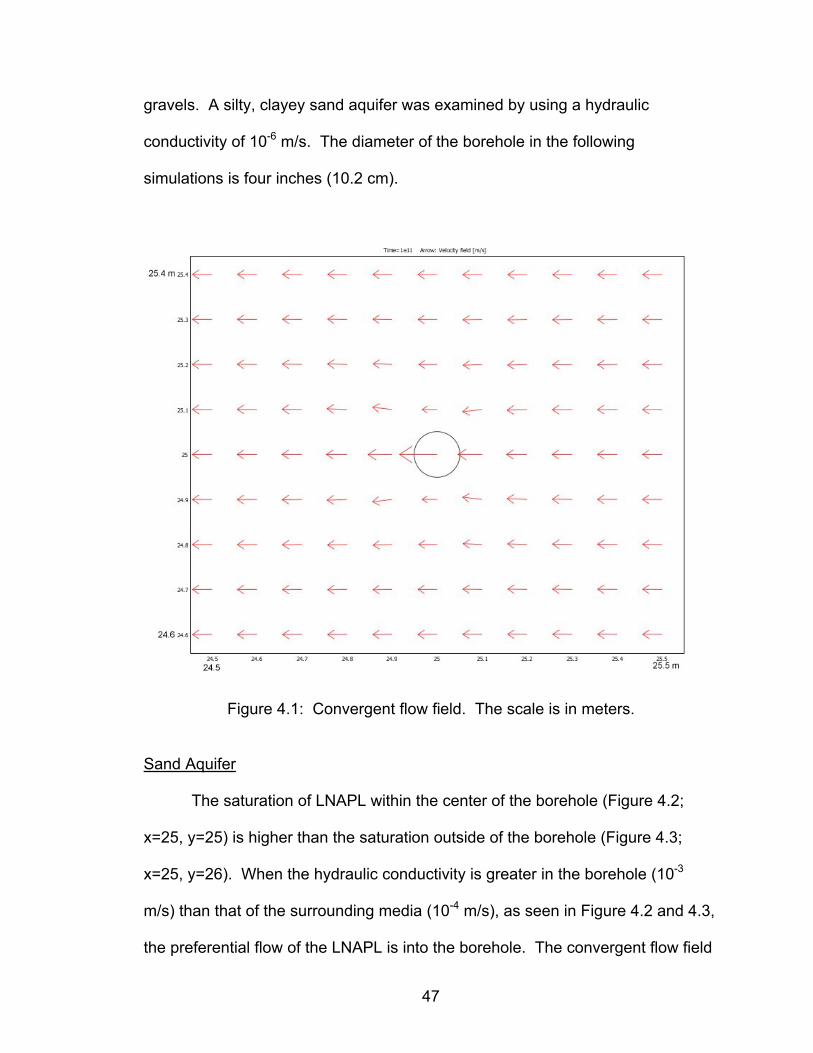
gravels. A silty, clayey sand aquifer was examined by using a hydraulic
conductivity of 10-6 m/s. The diameter of the borehole in the following
simulations is four inches (10.2 cm).
Figure 4.1: Convergent flow field. The scale is in meters.
Sand Aquifer
The saturation of LNAPL within the center of the borehole (Figure 4.2;
x=25, y=25) is higher than the saturation outside of the borehole (Figure 4.3;
x=25, y=26). When the hydraulic conductivity is greater in the borehole (10-3
m/s) than that of the surrounding media (10-4 m/s), as seen in Figure 4.2 and 4.3,
the preferential flow of the LNAPL is into the borehole. The convergent flow field
47
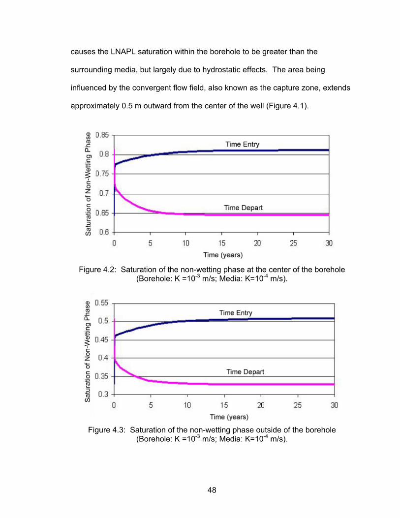
causes the LNAPL saturation within the borehole to be greater than the
surrounding media, but largely due to hydrostatic effects. The area being
influenced by the convergent flow field, also known as the capture zone, extends
approximately 0.5 m outward from the center of the well (Figure 4.1).
Figure 4.2: Saturation of the non-wetting phase at the center of the borehole
(Borehole: K =10-3 m/s; Media: K=10-4 m/s).
Figure 4.3: Saturation of the non-wetting phase outside of the borehole
(Borehole: K =10-3 m/s; Media: K=10-4 m/s).
48
When the non-wetting phase enters the borehole the LNAPL reaches
equilibrium between the well and surrounding porous media in approximately 21
years (Figure 4.2). As LNAPL departs the borehole equilibrium is once again
reached after 13 years. A similar pattern is seen outside of the borehole (Figure
4.3).
Silty, Clayey Sand Aquifer
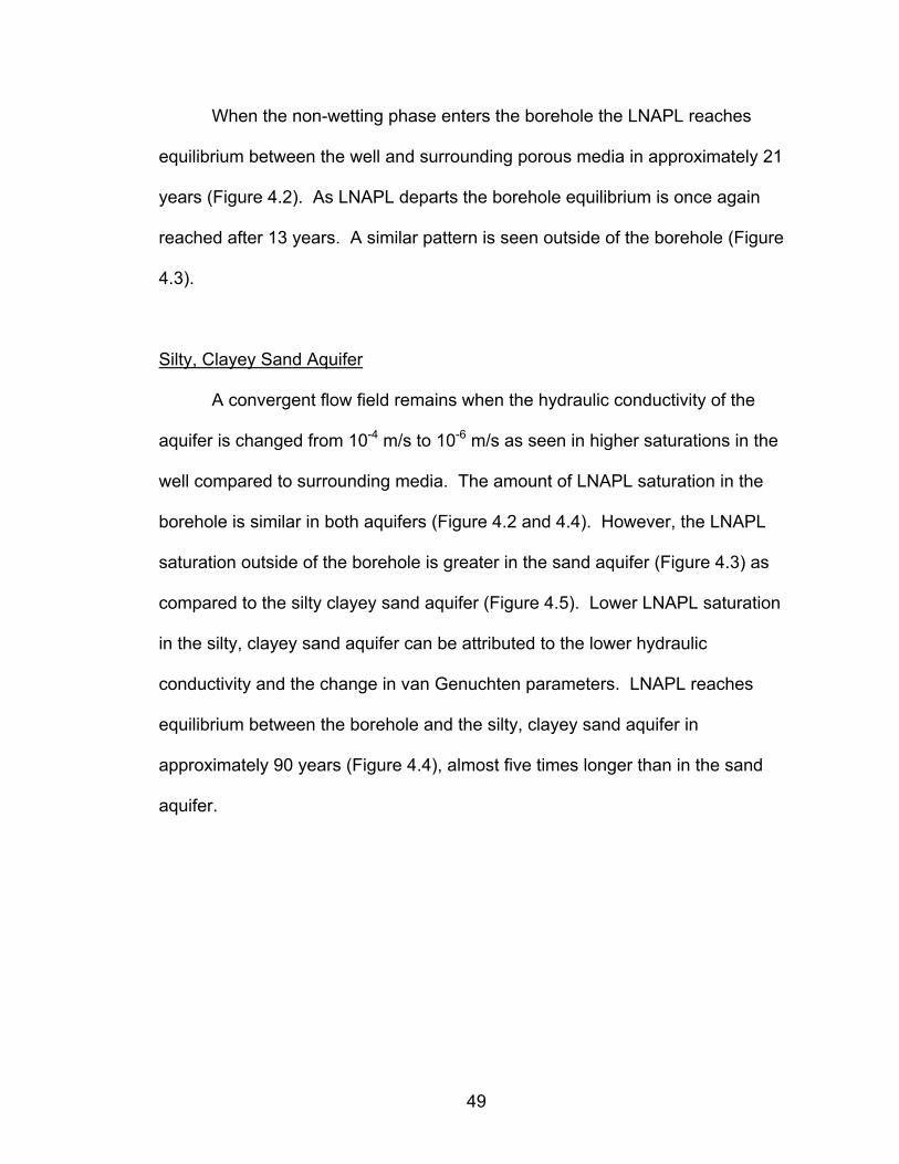
A convergent flow field remains when the hydraulic conductivity of the
aquifer is changed from 10-4 m/s to 10-6 m/s as seen in higher saturations in the
well compared to surrounding media. The amount of LNAPL saturation in the
borehole is similar in both aquifers (Figure 4.2 and 4.4). However, the LNAPL
saturation outside of the borehole is greater in the sand aquifer (Figure 4.3) as
compared to the silty clayey sand aquifer (Figure 4.5). Lower LNAPL saturation
in the silty, clayey sand aquifer can be attributed to the lower hydraulic
conductivity and the change in van Genuchten parameters. LNAPL reaches
equilibrium between the borehole and the silty, clayey sand aquifer in
approximately 90 years (Figure 4.4), almost five times longer than in the sand
aquifer.
49
Figure 4.4: Saturation of the non-wetting phase at the center of the borehole
(Borehole: K =10-3 m/s; Media: K=10-6 m/s).
Figure 4.5: Saturation of the non-wetting phase outside of the borehole
(Borehole: K =10-3 m/s; Media: K=10-6 m/s).
Divergent Flow Field
A divergent flow field is created around a borehole when the hydraulic
conductivity of the borehole is less than the surrounding media (Figure 4.6). A
50
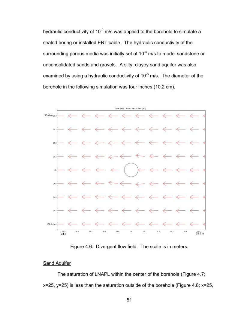
hydraulic conductivity of 10-9 m/s was applied to the borehole to simulate a
sealed boring or installed ERT cable. The hydraulic conductivity of the
surrounding porous media was initially set at 10-4 m/s to model sandstone or
unconsolidated sands and gravels. A silty, clayey sand aquifer was also
examined by using a hydraulic conductivity of 10-6 m/s. The diameter of the
borehole in the following simulation was four inches (10.2 cm).
Figure 4.6: Divergent flow field. The scale is in meters.
Sand Aquifer
The saturation of LNAPL within the center of the borehole (Figure 4.7;
x=25, y=25) is less than the saturation outside of the borehole (Figure 4.8; x=25,
51
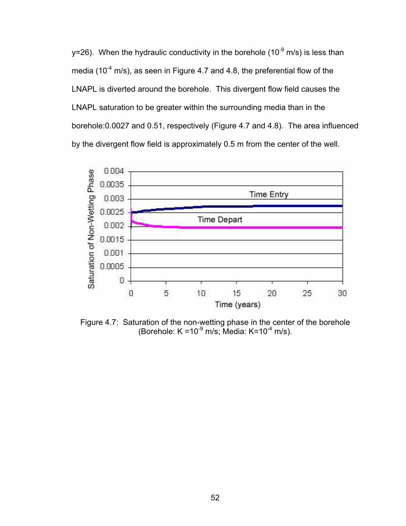
y=26). When the hydraulic conductivity in the borehole (10-9 m/s) is less than
media (10-4 m/s), as seen in Figure 4.7 and 4.8, the preferential flow of the
LNAPL is diverted around the borehole. This divergent flow field causes the
LNAPL saturation to be greater within the surrounding media than in the
borehole:0.0027 and 0.51, respectively (Figure 4.7 and 4.8). The area influenced
by the divergent flow field is approximately 0.5 m from the center of the well.
Figure 4.7: Saturation of the non-wetting phase in the center of the borehole
(Borehole: K =10-9 m/s; Media: K=10-4 m/s).
52
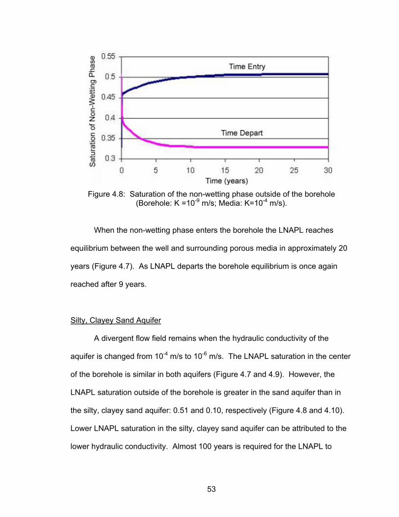
Figure 4.8: Saturation of the non-wetting phase outside of the borehole
(Borehole: K =10-9 m/s; Media: K=10-4 m/s).
When the non-wetting phase enters the borehole the LNAPL reaches
equilibrium between the well and surrounding porous media in approximately 20
years (Figure 4.7). As LNAPL departs the borehole equilibrium is once again
reached after 9 years.
Silty, Clayey Sand Aquifer
A divergent flow field remains when the hydraulic conductivity of the
aquifer is changed from 10-4 m/s to 10-6 m/s. The LNAPL saturation in the center
of the borehole is similar in both aquifers (Figure 4.7 and 4.9). However, the
LNAPL saturation outside of the borehole is greater in the sand aquifer than in
the silty, clayey sand aquifer: 0.51 and 0.10, respectively (Figure 4.8 and 4.10).
Lower LNAPL saturation in the silty, clayey sand aquifer can be attributed to the
lower hydraulic conductivity. Almost 100 years is required for the LNAPL to
53
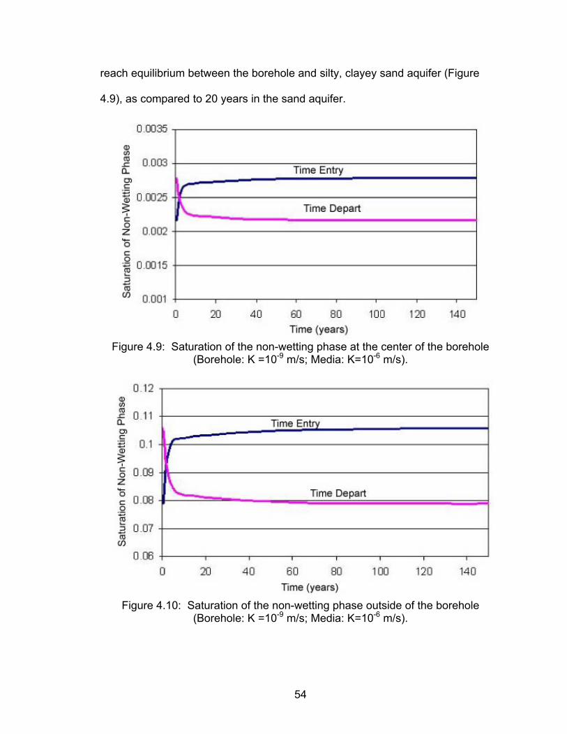
reach equilibrium between the borehole and silty, clayey sand aquifer (Figure
4.9), as compared to 20 years in the sand aquifer.
Figure 4.9: Saturation of the non-wetting phase at the center of the borehole
(Borehole: K =10-9 m/s; Media: K=10-6 m/s).
Figure 4.10: Saturation of the non-wetting phase outside of the borehole
(Borehole: K =10-9 m/s; Media: K=10-6 m/s).
54
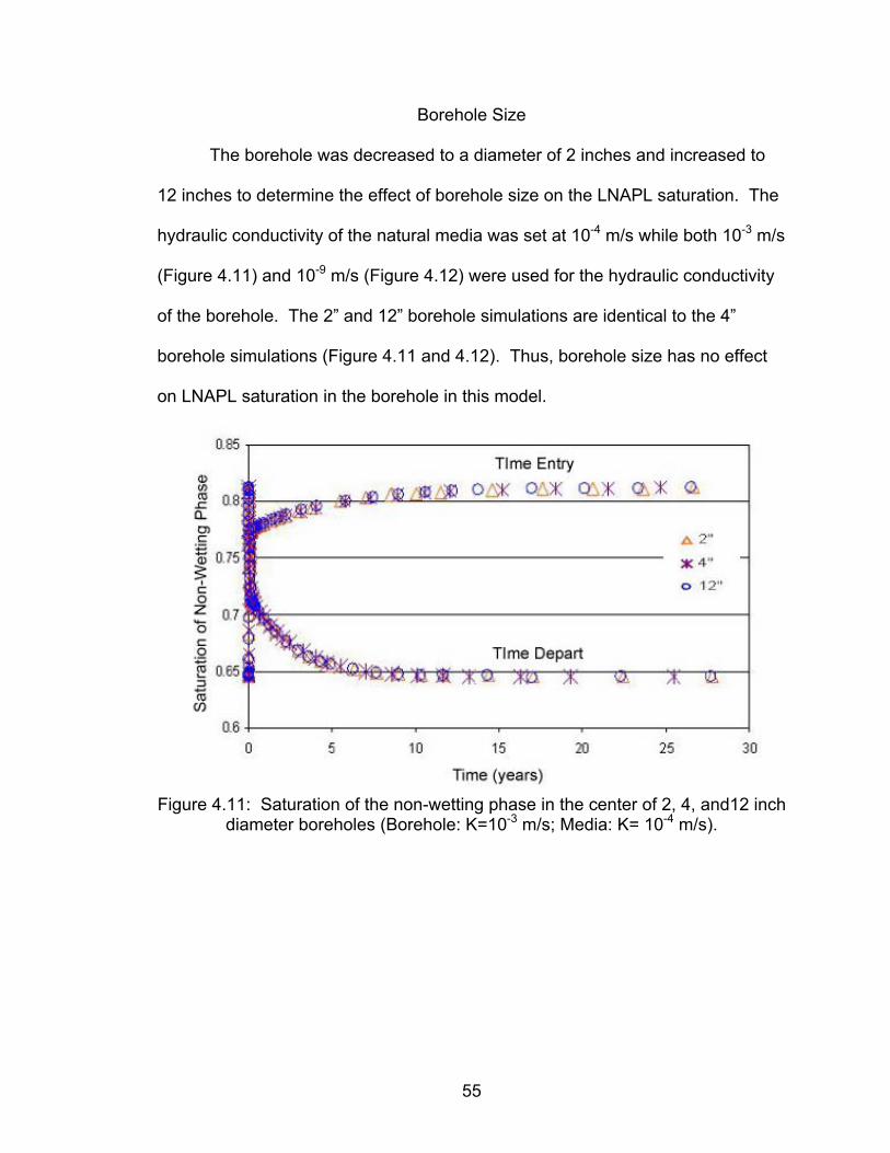
Borehole Size
The borehole was decreased to a diameter of 2 inches and increased to
12 inches to determine the effect of borehole size on the LNAPL saturation. The
hydraulic conductivity of the natural media was set at 10-4 m/s while both 10-3 m/s
(Figure 4.11) and 10-9 m/s (Figure 4.12) were used for the hydraulic conductivity
of the borehole. The 2” and 12” borehole simulations are identical to the 4”
borehole simulations (Figure 4.11 and 4.12). Thus, borehole size has no effect
on LNAPL saturation in the borehole in this model.
Figure 4.11: Saturation of the non-wetting phase in the center of 2, 4, and12 inch
diameter boreholes (Borehole: K=10-3 m/s; Media: K= 10-4 m/s).
55
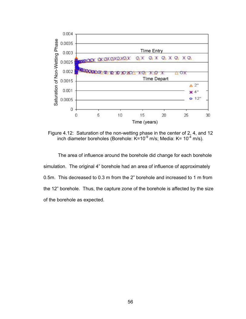
Figure 4.12: Saturation of the non-wetting phase in the center of 2, 4, and 12
inch diameter boreholes (Borehole: K=10-9 m/s; Media: K= 10-4 m/s).
The area of influence around the borehole did change for each borehole
simulation. The original 4” borehole had an area of influence of approximately
0.5m. This decreased to 0.3 m from the 2” borehole and increased to 1 m from
the 12” borehole. Thus, the capture zone of the borehole is affected by the size
of the borehole as expected.
56
CHAPTER V
DISCUSSION
The field data collected from the Enid, Golden, and Hobart, OK sites will
be compared to each other and to the modeling results. Implications from
modeling results regarding the length of time in which a well and formation reach
equilibrium in a two-phase system will be discussed. Finally, limitations to the
application of the model results to field sites are addressed.
Comparison of Field and Model Results
The Enid site was the only field site where free product was observed in
the monitoring wells (Figure 1.4), and was the only site that had monitoring wells
located in a relatively uniform sand layer. However, these wells are not located
in the plane of the resistivity images (Figure 1.3) but just north of the monitoring
electrodes (Figure 1.2). LNAPL is likely converging into these wells due to
pumping of the wells. Over time, LNAPL thickness in the monitoring wells
decreased with the exception of one well (Figure 1.4). Decreased thickness of
LNAPL in monitoring wells 17, 19, and 21 is mostly likely attributed to pumping
efforts for remediation. The increase in product thickness in MW-18 is likely
related to LNAPL coming from the south side of the site observed in ERI images
and in core data collected in July to August 2003. The LNAPL coming on to the
57
site was a separate segment from the “plume” delineated during the initial site
characterization.
The divergence from the electrode borings filled with bentonite may be
partially due to the divergence effect modeled in this thesis. However, the effects
observed in the COMSOL model were too small to explain the 2 – 3 m
conductive regions on either side of the electrode wells. A higher gradient due to
active pumping may explain the scale of the conductive regions, but has not
been tested with the current model.
LNAPL thickness from wells at the Golden, OK site do not correlate with
data from core sampling or ERI as the wells that correlated with ERI images had
no detectable LNAPL. LNAPL blobs can be observed between the wells in
electrical images (Figure 1.8). The presence of LNAPL was confirmed by soil
borings (Halihan et al., 2005a). However, no free product was observed in the
wells. The wells may not record free product since they were used for
remediation (i.e., injection and extraction). Figure 1.8 shows LNAPL blobs
moving toward to Well 16, which is an extraction well (Halihan et al., 2005a).
LNAPL moves away from wells 48, 46, 52 and 50 because they are injection
wells. Modeling results may not provide the mechanism to explain this site since
a higher hydraulic gradient exists during remediation efforts. The observed scale
of separation from the wells indicates that the modeled mechanism is not large
enough to generate the LNAPL free zones around the wells.
An expected convergent flow field around the wells was not observed at
the Hobart, OK site. The monitoring wells have filter packs consisting of 20/40
58
silica sand and the wells are sealed with bentonite chips above the screened
intervals. The stratigraphy of this site (Table 1.3) predominantly consists of silty
clay. Thus, the well has a higher hydraulic conductivity than the surrounding
media which should cause a convergent flow field. From the modeling results,
we would predict that the monitoring wells would be highly saturated with LNAPL
(Figure 4.4). However, no hydrocarbon was measured in the monitoring wells.
ERI and core data indicated that LNAPL contamination was present around the
wells. A divergent flow field may be preventing LNAPL from entering the
monitoring wells. Such a flow field could have been created by smearing when
the well was drilled using an auger rig. As the well was drilled into the silty clay,
the clay could have been smeared along the sides of the borehole. This would
cause a skin effect which is preventing LNAPL migration into the well. The wells
could have also been poorly developed which is causing the wells to not be open
to surrounding media. An additional explanation provided by the COMSOL
model is that the aquifer is not in equilibrium with the well as the model
suggested that it may take several tens of years to reach equilibrium with the
formation.
Overall, our model does not fully explain the reasons that LNAPL
thickness measurements in wells do not correlate to ERI images and soil cores at
these field sites. The model predicted convergent flow fields to be observed
around wells at all of the sites. The field data did not correspond to the model
prediction however, other factors such as high gradients due to pumping, poorly
developed wells, and remediation efforts were at play. The model results do
59
indicate that the hydraulic conductivity contrast between the borehole and natural
media is one more variable that may cause differences between LNAPL
thickness measurements in wells and the surrounding media.
Equilibrium Time Scales
Our model did provide an estimate for the time equilibrium is reached
between a borehole and the surrounding media in a two-phase system. Under
an ambient hydraulic gradient, equilibrium is reached between 7 - 11 years after
LNAPL was introduced into the system (Figure 5.1) at a small site of 50x50
meters. When LNAPL was forced to depart, the borehole equilibrium was
reached from 5 - 7 years (Figure 5.1). Therefore, using an assumption of
hydrostatic conditions may not be valid since the time in which equilibrium is
reached under ambient gradients is longer than the time spent on typical site
characterization and remediation projects. This indicates that hydrodynamic
conditions within a borehole and surrounding media will never be reached, and
transient conditions must be accounted for when correlating well data with
formation data. For most sites, this data will not be available.
60
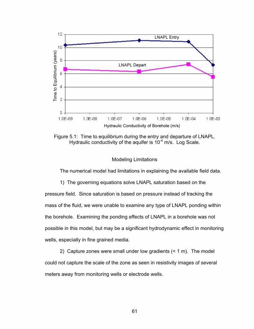
Figure 5.1: Time to equilibrium during the entry and departure of LNAPL.
Hydraulic conductivity of the aquifer is 10-4 m/s. Log Scale.
Modeling Limitations
The numerical model had limitations in explaining the available field data.
1) The governing equations solve LNAPL saturation based on the
pressure field. Since saturation is based on pressure instead of tracking the
mass of the fluid, we were unable to examine any type of LNAPL ponding within
the borehole. Examining the ponding effects of LNAPL in a borehole was not
possible in this model, but may be a significant hydrodynamic effect in monitoring
wells, especially in fine grained media.
2) Capture zones were small under low gradients (< 1 m). The model
could not capture the scale of the zone as seen in resistivity images of several
meters away from monitoring wells or electrode wells.
61
3) Monitoring wells were expected to read higher thicknesses of LNAPL in
fine grained media. At our field sites, we did not detect LNAPL in contaminated
areas from monitoring wells which may be due to a skin effect generated by
auger rotation in a fine grained formation, or a lack of time to reach equilibrium
which the model suggests may be years.
Future modeling efforts could be improved with saturation data from the
field sites instead of only TPH data. Additionally, generating a model that
calculated saturation through mass tracking equations instead of pressure
equations may improve our understanding of monitoring well hydrodynamics.
62
CHAPTER VI
CONCLUSIONS
The major findings generated through the study of ERI, core samples,
monitoring wells measurements and two-phase modeling:
1) Previous efforts to model the interaction of two-phase flow and
monitoring wells indicate that wells are difficult to correlate to aquifer
conditions under hydrostatic considerations. Factors affecting LNAPL
thickness measurements in a well include multiphase interaction, capillary
pressure, ground water table fluctuations, sediment variability, and pore size
distribution.
2) Electrical resistivity imaging suggests that boreholes are interacting
with the flow field. Resistive areas in ERI data that are correlated to the
presence of LNAPL in the formation are either attracted to or repelled from
monitoring points on a scale of several meters.
3) A hydraulic conductivity contrast between a borehole and
surrounding porous media affect a two-phase flow field. When the hydraulic
conductivity is greater in the borehole than the surrounding media a
convergent flow field is formed. A divergent flow field is formed when the
hydraulic conductivity of the borehole is less than the surrounding media.
63

This effect can lead to inaccurate LNAPL thickness measurements taken from
a monitoring well.
4) Borehole modeling suggests hydrodynamic equilibrium may not be
reached with the surrounding porous media. Model results show the time it
can take for a borehole and the surrounding media to reach equilibrium can
range from 9 to 23 years in an aquifer with a hydraulic conductivity of 10-4 m/s
and even longer for lower conductivity materials.
5) Borehole modeling suggests that capture zones for monitoring wells
or repulsion zones for installed electrode strings under ambient gradients are
small, generally less than a meter. This suggests that a larger scale
mechanism is required to explain ERI and core data.
64
REFERENCES
Adamski, M., Charbeneau, R.J., and Kuhn, J. 2007. LNAPL in the subsurface:
recent developments, new conceptual models, and new tools. 19th Annual Tanks Conference & Expo, San Antonio, TX. p. 1-77.
Adamski, M., Kremesec, V., Kolhatkar, R., Pearson, C., and Rowan, B. 2005.
LNAPL in fine-grained soils: conceptualization of saturation, distribution, recovery, and their modeling. Ground Water Monitoring & Remediation. 25:100-112.
Aestus, LLC. 2004. Report of GeoTrax SurveyTM Work, Department of Human
Health Services Site, Hobart, OK. p.1-27. Aral, M.M., and Liao, B. 2002. Effect of groundwater table fluctuations on
LNAPL thickness in monitoring wells. Environmental Geology. 42:151-161.
Atekwana, E.A., Sauck, W.A., Werkema Jr., D.D. 2000. Investigations of
geoelectrical signatures at a hydrocarbon contaminated site. Journal of Applied Geophysics. 44:167-180.
Ballestero, T.P., Fiedler, F.R., and Kinner, N.E. 1994. An investigation of the
relationship between actual and apparent gasoline thickness in a uniform sand aquifer. Ground Water. 32:708-718.
Beckett, G.D. and Huntley, D. 1998. Soil properties and design factors
influencing free-phase hydrocarbon cleanup. Environmental Science and Technology. 32:287-293.
Benson, A.K. and Mustoe, N.B. 1996. DC resistivity, ground-penetrating radar,
and soil and water quality data combined to assess hydrocarbon contamination: A case study in Arizona. Environmental Geosciences. 3:165-175.
Brooks, R.H. and Corey, A.T. 1964. Hydraulic properties of porous media.
Hydrology, Paper 3, Colorado State University, Fort Collins, CO.
65
Carsell, R.F. and Parish, R.S. 1988. Developing joint probability distributions of soil water retention characteristics. Water Resources Research. 24:755-769.
Charbeneau, R.J. 2000. Groundwater Hydraulics and Pollutant Transport.
Prentice Hall, New Jersey. p.1-594. Charbeneau, R.J., Johns, R.T., Lake, L.W., and McAdams III, M.J. 1999. Free-
Product Recovery of Petroleum Hydrocarbon Liquids. API Publication Number 4682. American Petroleum Institute, Washington, D.C. p.1.1-6.6.
Charbeneau, R.J., Johns, R.T., Lake, L.W., and McAdams III, M.J. 2000. Free-
product recovery of petroleum hydrocarbon liquids. Ground Water Monitoring & Remediation. 20:147-158.
COMSOL Multiphysics. 2005. Earth Science Module; Model Library. 2:133-154. Daily, W., Ramirez, A., LaBrecque, D., and Barber, W. 1995. Electrical
resistance tomography experiments at the Oregon Graduate Institute. Journal of Applied Geophysics. 33:227-237.
de Marsily, Ghislain. 1986. Quantitative Hydrogeology: Groundwater Hydrology
for Engineers. Academic Press, Inc., Florida. Dahlberg, E.C. 1995. Applied Hydrodynamics in Petroleum Exploration.
Springer-Verlag, New York. p.1-14. Delaney, A.J., Peapples, P.R., and Arcone, S.A. 2001. Electrical resistivity of
frozen and petroleum-contaminated fine-grained soil. Cold Regions Science and Technology. 32:107-119.
Driscoll, F.G. 1986. Groundwater and Wells. 2nd. ed. Johnson Filtration
Systems Inc., St. Paul, Minnesota. p.438-483. Farr, A.M., Houghtalen, R.J., and McWhorter, D.B. 1990. Volume estimation of
light nonaqueous phase liquids in porous media. Ground Water. 28:48-56.
Fetter, C.W. 2001. Applied Hydrogeology. 4th. ed. Prentice Hall, New Jersey.
p. 66-218. Gleason, M.H., Daniel, D.E., and Eykholt, G.R. 1997. Calcium and sodium
bentonite for hydraulic containment applications. Journal of Geotechnical and Geoenvironmental Engineering. 123:438-445.
66
Graham, I. 2007. Electrical Resistivity Imaging of a Remediated Gasoline Site in Golden, Oklahoma. Master of Science Thesis, Oklahoma State University, Stillwater, OK.
Grechka, V. and Soutter, L. 2005. Simulation of two-phase fluid flow through
compactible reservoirs. Geophysical Prospecting. 53:829-841. Halihan, T., Paxton, S., Graham, I., Fenstemaker, T., and Riley, M. 2005a.
Post-remediation evaluation of a LNAPL site using electrical resistivity imaging. Journal of Environmental Monitoring. 7:283-287.
Halihan, T., Paxton, S., Graham, I., and Riley M. 2005b. Final report of activities
for: Post remediation characterization of LNAPL using electrical resistivity and direct push techniques. Oklahoma Corporation Commission, Petroleum Storage Tank Division, Oklahoma City, OK. p.1-26.
Halihan, T., Paxton, S., McPhail, M., McSorley, J., and Riley, M. 2005c. Final
report for: Environmental characterization and monitoring of LNAPL using electrical resistivity tomography (ERT) and hydraulic push techniques. Oklahoma Corporation Commission, Petroleum Storage Tank Division, Oklahoma City, OK. p.1-74.
Herzog, B.L. 1994. Slug tests for determining hydraulic conductivity of natural
geologic deposits. In Daniel, D.E. and Trautwein, S.J. eds. Hydraulic Conductivity and Waste Contaminant Transport in Soil. 1994. American Society for Testing and Materials, Philadelphia, PA. p.95-110.
Huntley, D., Hawk, R.N., and Corley, H.P. 1994a. Nonaqueous phase
hydrocarbon in a fine-grained sandstone: 1. Comparison between measured and predicted saturations and mobility. Ground Water. 32:626-634.
Huntley, D., Wallace, J.W., and Hawk, R.N. 1994b. Nonaqueous phase
hydrocarbon in a fine-grained sandstone: 2. Effect of local sediment variability on the estimation of hydrocarbon volumes. Ground Water. 32:778-783.
Johnson, H.L. and Duchon, C.E. 1995. Atlas of Oklahoma Climate. University
of Oklahoma Press, Norman, OK. Kemblowski, M.W. and Chiang, C.Y. 1990. Hydrocarbon thickness fluctuations
in monitoring wells. Ground Water. 28:244-252.
67
Kemna, A., Vanderborght, J., Kulessa, B., and Vereecken, H. 2002. Imaging and characterization of subsurface solute transport using electrical resistivity tomography (ERT) and equivalent transport models. Journal of Hydrology. 267:125-146.
LaBrecque, D.J., Ramirez, A.L., Daily, W.D., Binley, A.M., and Schima, S.A.
1996. ERT monitoring of environmental remediation processes. Measurement Science and Technology. 7:275-383.
Lenhard, R.J. 1990. Estimation of free hydrocarbon volume from fluid levels in
monitoring wells; and, volume estimation of light nonaqueous phase liquids in porous media; discussion. Ground Water. 28:800-801.
Lenhard, R.J., and Parker, J.C. 1990. Estimation of free hydrocarbon volume
from fluid levels in monitoring wells. Ground Water. 28:57-67. Liao, B., and Aral, M.M. 1999. Interpretation of LNAPL thickness measurements
under unsteady conditions. Journal of Hydrologic Engineering. p.125-134.
Loh, W.W., Waterfall, R.C., Cory, J., and Lucas, G.P. 1999. Using ERT for
multi-phase flow monitoring. 1st World Congress on Industrial Process Tomography, Buxton, Greater Manchester. p.47-53.
McPhail, M.L. 2003. Geological Controls on the Location and Distribution of an
LNAPL Plume at a Site in Enid, Oklahoma. Master of Science Thesis, Oklahoma State University, Stillwater, OK. p.1-137.
McSorley, J.D. 2003. Direct Push Electrical Resistivity Tomography to Detect
NAPL. Master of Science Thesis, Oklahoma State University, Stillwater, OK. p.1-149.
Mualem, Y. 1976. A new model for predicting the hydraulic permeability of
unsaturated porous media. Water Resources Research. 12:513-522. Secor International Incorporated. 2004. Kiowa County Department of Human
Services Final Report, Project No. 710T.08972.04. Sleep, B.E., Sehayek, L., and Chien, C.C. 2000. A modeling and experimental
study of light nonaqueous phase liquid (LNAPL) accumulation in wells and LNAPL recovery from wells. Water Resources Research. 36:3535-3545.
Thurston, R.N. 1974. Waves in solids. Encyclopedia of Physics, Mechanics of
Solids. 4:109-302.
68
van Genuchten, M.T. 1980. A closed-form equation for predicting the hydraulic conductivity of unsaturated soils. Soil Science Society of America Journal. 44:892-898.
Vogler, M., Arslan, P., and Katzenbach, R. 2001. The influence of capillarity on
multiphase flow within porous media: a new model for interpreting fluid levels in groundwater monitoring wells in dynamic aquifers. Engineering Geology. 60:149-158.
Wallace, J.W. and Huntley, D. 1992. Effect of local sediment variability on the
estimation of hydrocarbon volumes. Ground Water Management. 11:273-285.
Weight, W.D. and Sonderegger, J.L. 2001. Manual of Applied Field
Hydrogeology. McGraw-Hill. p.332-339.
69
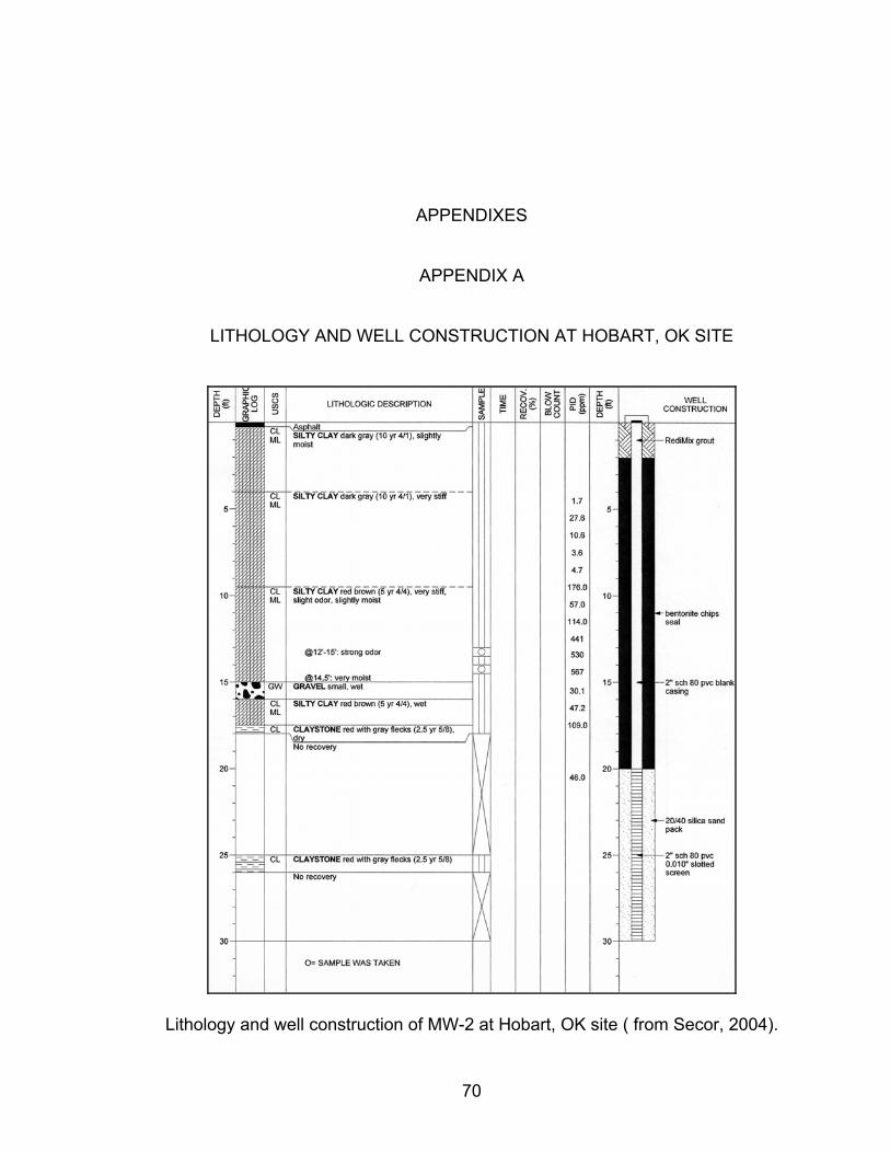
APPENDIXES
APPENDIX A
LITHOLOGY AND WELL CONSTRUCTION AT HOBART, OK SITE
Lithology and well construction of MW-2 at Hobart, OK site ( from Secor, 2004).
70
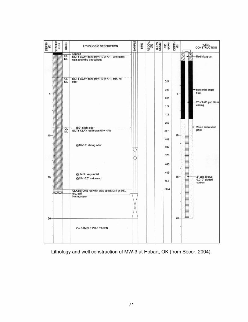
Lithology and well construction of MW-3 at Hobart, OK (from Secor, 2004).
71
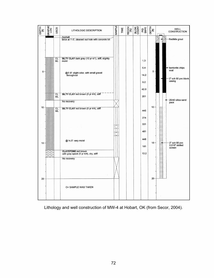
Lithology and well construction of MW-4 at Hobart, OK (from Secor, 2004).
72

APPENDIX B
COMSOL MULTIPHYSICS MODEL
COMSOL Multiphysics requires an extensive number of parameters to
model two-phase flow. The program provides an output to be able to reproduce
the model described in this thesis. This Appendix details the parameters used to
generate the model.
1. Table of Contents • Title - JT Thesis • Table of Contents • Model Properties • Constants • Geometry • Geom1 • Interpolation Functions • Solver Settings • Postprocessing • Variables
2. Model Properties Property Value Model name JT Thesis Author Jennifer Thorstad Company Oklahoma State UniversityDepartment School of Geology Reference URL Saved date Apr 16, 2007 6:03:14 PM Creation date Mar 14, 2007 10:03:20 PMCOMSOL version COMSOL 3.3.0.511
73
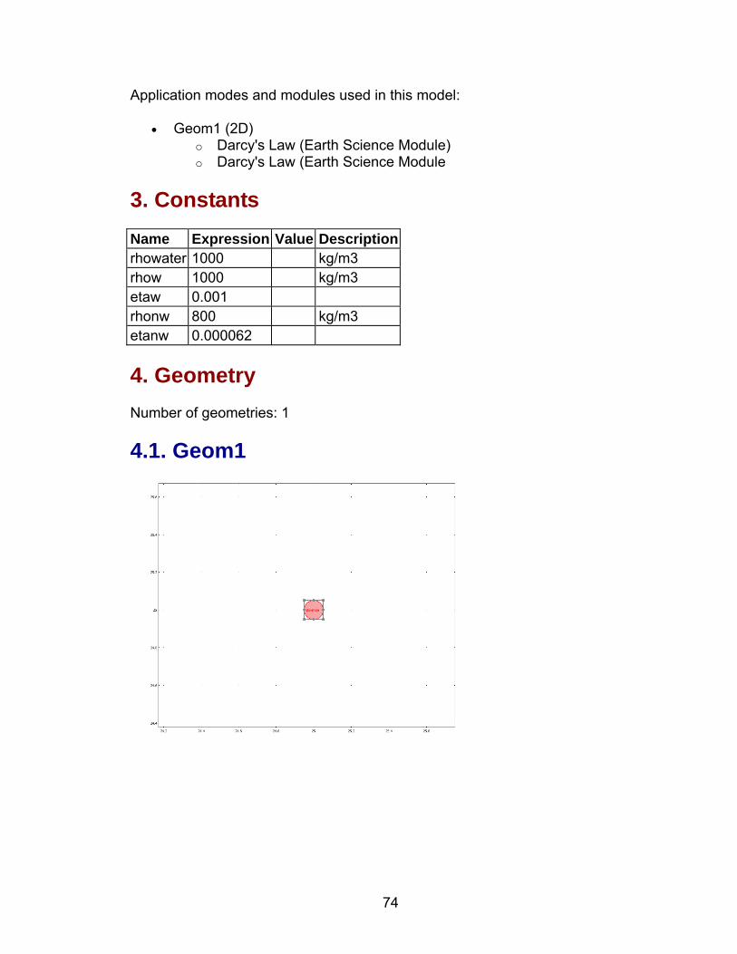
Application modes and modules used in this model:
• Geom1 (2D) o Darcy's Law (Earth Science Module) o Darcy's Law (Earth Science Module
3. Constants Name Expression Value Descriptionrhowater 1000 kg/m3 rhow 1000 kg/m3 etaw 0.001 rhonw 800 kg/m3 etanw 0.000062
4. Geometry Number of geometries: 1
4.1. Geom1
74
4.1.1. Point mode
4.1.2. Boundary mode
75
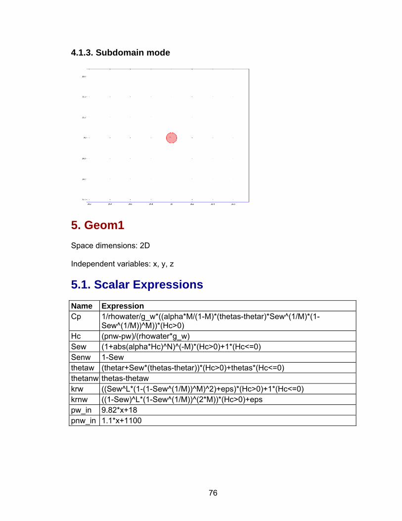
4.1.3. Subdomain mode
5. Geom1 Space dimensions: 2D
Independent variables: x, y, z
5.1. Scalar Expressions Name Expression Cp 1/rhowater/g_w*((alpha*M/(1-M)*(thetas-thetar)*Sew^(1/M)*(1-
Sew^(1/M))^M))*(Hc>0) Hc (pnw-pw)/(rhowater*g_w) Sew (1+abs(alpha*Hc)^N)^(-M)*(Hc>0)+1*(Hc<=0) Senw 1-Sew thetaw (thetar+Sew*(thetas-thetar))*(Hc>0)+thetas*(Hc<=0) thetanw thetas-thetaw krw ((Sew^L*(1-(1-Sew^(1/M))^M)^2)+eps)*(Hc>0)+1*(Hc<=0) krnw ((1-Sew)^L*(1-Sew^(1/M))^(2*M))*(Hc>0)+eps pw_in 9.82*x+18 pnw_in 1.1*x+1100
76
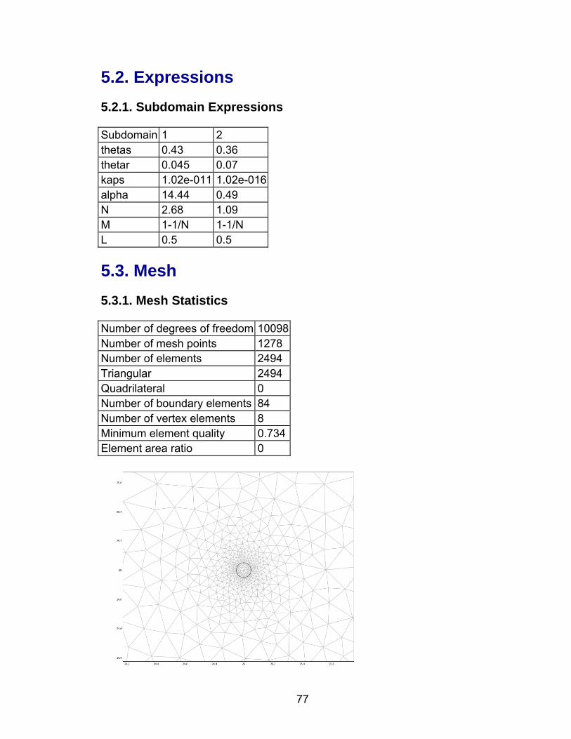
5.2. Expressions 5.2.1. Subdomain Expressions
Subdomain 1 2 thetas 0.43 0.36 thetar 0.045 0.07 kaps 1.02e-011 1.02e-016alpha 14.44 0.49 N 2.68 1.09 M 1-1/N 1-1/N L 0.5 0.5
5.3. Mesh 5.3.1. Mesh Statistics
Number of degrees of freedom 10098Number of mesh points 1278 Number of elements 2494 Triangular 2494 Quadrilateral 0 Number of boundary elements 84 Number of vertex elements 8 Minimum element quality 0.734Element area ratio 0
77
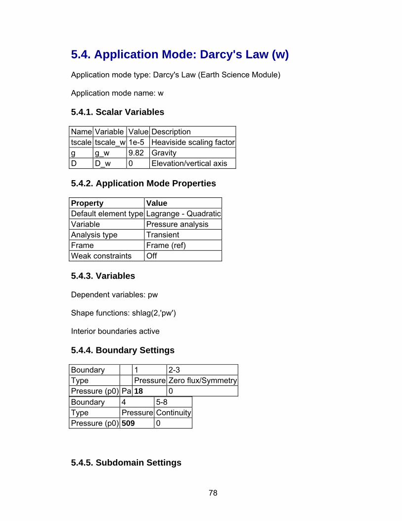
5.4. Application Mode: Darcy's Law (w) Application mode type: Darcy's Law (Earth Science Module)
Application mode name: w
5.4.1. Scalar Variables
Name Variable Value Description tscale tscale_w 1e-5 Heaviside scaling factorg g_w 9.82 Gravity D D_w 0 Elevation/vertical axis
5.4.2. Application Mode Properties
Property Value Default element type Lagrange - QuadraticVariable Pressure analysis Analysis type Transient Frame Frame (ref) Weak constraints Off
5.4.3. Variables
Dependent variables: pw
Shape functions: shlag(2,'pw')
Interior boundaries active
5.4.4. Boundary Settings
Boundary 1 2-3 Type Pressure Zero flux/SymmetryPressure (p0) Pa 18 0 Boundary 4 5-8 Type Pressure ContinuityPressure (p0) 509 0
5.4.5. Subdomain Settings
78
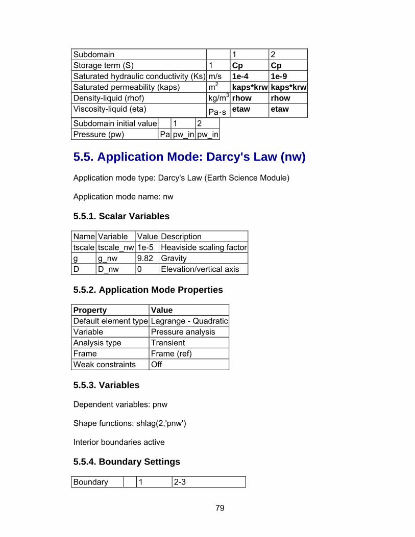
Subdomain 1 2 Storage term (S) 1 Cp Cp Saturated hydraulic conductivity (Ks) m/s 1e-4 1e-9 Saturated permeability (kaps) m2 kaps*krw kaps*krw Density-liquid (rhof) kg/m3 rhow rhow Viscosity-liquid (eta) Pa·s etaw etaw
Subdomain initial value 1 2 Pressure (pw) Pa pw_in pw_in
5.5. Application Mode: Darcy's Law (nw) Application mode type: Darcy's Law (Earth Science Module)
Application mode name: nw
5.5.1. Scalar Variables
Name Variable Value Description tscale tscale_nw 1e-5 Heaviside scaling factorg g_nw 9.82 Gravity D D_nw 0 Elevation/vertical axis
5.5.2. Application Mode Properties
Property Value Default element type Lagrange - QuadraticVariable Pressure analysis Analysis type Transient Frame Frame (ref) Weak constraints Off
5.5.3. Variables
Dependent variables: pnw
Shape functions: shlag(2,'pnw')
Interior boundaries active
5.5.4. Boundary Settings
Boundary 1 2-3
79
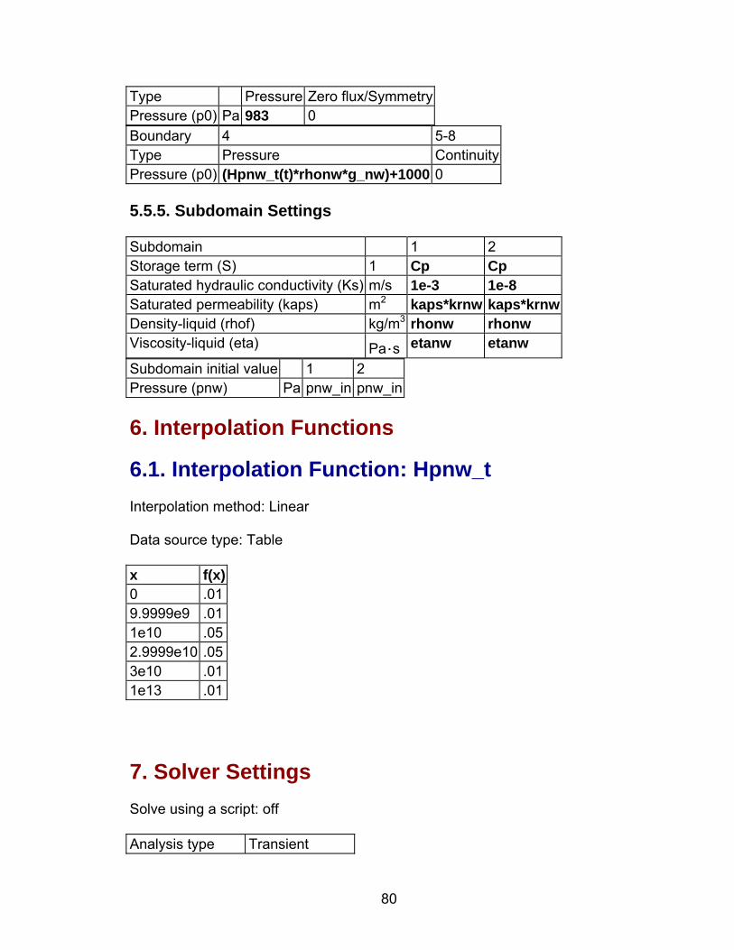
Type Pressure Zero flux/SymmetryPressure (p0) Pa 983 0 Boundary 4 5-8 Type Pressure ContinuityPressure (p0) (Hpnw_t(t)*rhonw*g_nw)+1000 0
5.5.5. Subdomain Settings
Subdomain 1 2 Storage term (S) 1 Cp Cp Saturated hydraulic conductivity (Ks) m/s 1e-3 1e-8 Saturated permeability (kaps) m2 kaps*krnw kaps*krnw Density-liquid (rhof) kg/m3 rhonw rhonw Viscosity-liquid (eta) Pa·s etanw etanw
Subdomain initial value 1 2 Pressure (pnw) Pa pnw_in pnw_in
6. Interpolation Functions
6.1. Interpolation Function: Hpnw_t Interpolation method: Linear
Data source type: Table
x f(x) 0 .01 9.9999e9 .01 1e10 .05 2.9999e10 .05 3e10 .01 1e13 .01
7. Solver Settings Solve using a script: off
Analysis type Transient
80
Auto select solver On Solver Time dependentSolution form General Symmetric auto Adaption Off
7.1. Direct (UMFPACK) Solver type: Linear system solver
Parameter ValuePivot threshold 0.1 Memory allocation factor 0.7
7.2. Time Stepping Parameter Value Times 0:1e9:1e11 Relative tolerance 0.004 Absolute tolerance 0.0005 Times to store in output Time steps from solver Time steps taken by solver Free Manual tuning of step size Off Initial time step 0.0010 Maximum time step 1.0 Maximum BDF order 5 Singular mass matrix Maybe Consistent initialization of DAE systems Off Error estimation strategy Include algebraic Allow complex numbers Off
7.3. Advanced Parameter Value Constraint handling method EliminationNull-space function Automatic
81
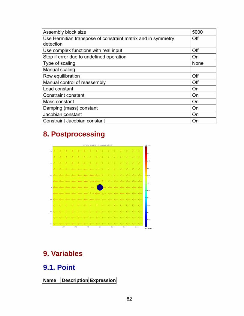
Assembly block size 5000 Use Hermitian transpose of constraint matrix and in symmetry detection
Off
Use complex functions with real input Off Stop if error due to undefined operation On Type of scaling None Manual scaling Row equilibration Off Manual control of reassembly Off Load constant On Constraint constant On Mass constant On Damping (mass) constant On Jacobian constant On Constraint Jacobian constant On
8. Postprocessing
9. Variables
9.1. Point Name Description Expression
82
rhof_w Density rhow rhof_nw Density rhonw
9.2. Boundary Name Description Expression nU_w Normal velocity u_w * nx_w+v_w * ny_w flux_w Outward flux u_w * nx_w+v_w * ny_w nU_nw Normal velocity u_nw * nx_nw+v_nw * ny_nwflux_nw Outward flux u_nw * nx_nw+v_nw * ny_nw
9.3. Subdomain Name Description Expression S_w Storage term Cp * CSs_w Qs_w Liquid source 0 K_w Hydraulic
conductivity tensor
Ks_w * CKs_w
Kxx_w Hydraulic conductivity tensor
K_w
Kxy_w Hydraulic conductivity tensor
0
Kyx_w Hydraulic conductivity tensor
0
Kyy_w Hydraulic conductivity tensor
K_w
kap_w Permeability tensor
kaps_w * CKs_w
kapxx_w Permeability tensor
kap_w
kapxy_w Permeability tensor
0
kapyx_w Permeability tensor
0
kapyy_w Permeability tensor
kap_w
gradP_w Pressure gradient sqrt(pwx^2+pwy^2)
83
u_w x-velocity (-kapxx_w * (pwx+diff(rhof_w * g_w * D_w,x))-kapxy_w * (pwy+diff(rhof_w * g_w * D_w,y)))/eta_w
v_w y-velocity (-kapyx_w * (pwx+diff(rhof_w * g_w * D_w,x))-kapyy_w * (pwy+diff(rhof_w * g_w * D_w,y)))/eta_w
U_w Velocity field sqrt(u_w^2+v_w^2) S_nw Storage term Cp * CSs_nw Qs_nw Liquid source 0 K_nw Hydraulic
conductivity tensor
Ks_nw * CKs_nw
Kxx_nw Hydraulic conductivity tensor
K_nw
Kxy_nw Hydraulic conductivity tensor
0
Kyx_nw Hydraulic conductivity tensor
0
Kyy_nw Hydraulic conductivity tensor
K_nw
kap_nw Permeability tensor
kaps_nw * CKs_nw
kapxx_nw Permeability tensor
kap_nw
kapxy_nw Permeability tensor
0
kapyx_nw Permeability tensor
0
kapyy_nw Permeability tensor
kap_nw
gradP_nw Pressure gradient sqrt(pnwx^2+pnwy^2) u_nw x-velocity (-kapxx_nw * (pnwx+diff(rhof_nw * g_nw *
D_nw,x))-kapxy_nw * (pnwy+diff(rhof_nw * g_nw * D_nw,y)))/eta_nw
v_nw y-velocity (-kapyx_nw * (pnwx+diff(rhof_nw * g_nw * D_nw,x))-kapyy_nw * (pnwy+diff(rhof_nw * g_nw * D_nw,y)))/eta_nw
U_nw Velocity field sqrt(u_nw^2+v_nw^2)
84
VITA
Jennifer L. Thorstad
Candidate for the Degree of
Master of Science Thesis: INFLUENCE OF BOREHOLE CONSTRUCTION ON LNAPL
THICKNESS MEASUREMENTS Major Field: Geology Biographical:
Personal Data: Born on April 17, 1983 in Alexandria, MN. Grew up east of Hoffman, MN.
Education: Graduated from West Central Area Secondary Schools,
Barrett, MN in May 2001. Received Bachelor of Science in Geology from North Dakota State University, Fargo, ND in May 2005. Completed the requirements for the Master of Science degree in Geology at Oklahoma State University in May 2007.
Experience: Employed by Oklahoma State University School of Geology
as a teaching assistant from 2005 to 2007. Professional Memberships: Geological Society of America
Name: Jennifer L. Thorstad Date of Degree: May, 2007 Institution: Oklahoma State University Location: Stillwater, Oklahoma Title of Study: INFLUENCE OF BOREHOLE CONSTRUCTION ON LNAPL
THICKNESS MEASUREMENTS Pages in Study: 84 Candidate for the Degree of Master of Science
Major Field: Geology Abstract: Electrical resistivity images taken at sites contaminated by gasoline or
light non-aqueous phase liquids (LNAPL) often image LNAPL being affected by the location of boreholes as either an attractive or repulsive feature in the subsurface. This mechanism results in an anomalously low or high estimate of the amount of LNAPL in the formation using data sampled from wells. The field data suggest that in fine grained media LNAPL may not be detected by monitoring wells. A numerical model was constructed to determine if the hydraulic conductivity contrast between a borehole and natural media has a significant enough effect to create either a convergent or divergent two-phase flow field around a borehole which would lead to inaccurate LNAPL measurements. The model results indicate that ambient gradients are not sufficient to create the observed geophysical effect, but do demonstrate that the wells may never reach equilibrium with the formation.
ADVISOR’S APPROVAL: Dr. Todd Halihan