RELATIONSHIPS AMONG GEOMORPHOLOGY,

HABITAT, AND FISHES IN EASTERN OKLAHOMA

STREAMS: IMPLICATIONS FOR STREAM

RESTORATION

By

DANIEL CARL DAUWALTER

Bachelor of Arts Gustavus Adolphus College

St. Peter, Minnesota 1999

Master of Science

University of Arkansas at Pine Bluff Pine Bluff, Arkansas

2002

Submitted to the Faculty of the Graduate College of Oklahoma State University in partial fulfillment of

the requirements for the degree of DOCTOR OF PHILOSOPHY

May, 2006

RELATIONSHIPS AMONG GEOMORPHOLOGY,

HABITAT, AND FISHES IN EASTERN OKLAHOMA

STREAMS: IMPLICATIONS FOR STREAM

RESTORATION

Dissertation Approved: William L. Fisher

Dissertation Advisor Richard A. Marston Anthony A. Echelle Joseph R. Bidwell A. Gordon Emslie

Dean of the Graduate College

ii

PREFACE

All chapters of this dissertation were written as manuscripts that will be submitted to

peer-reviewed journals. Therefore, each chapter follows the style and guidelines of the

respective journal to which it will be submitted: Chapter 1, Ecology of Freshwater Fish;

Chapter 2, Canadian Journal of Fisheries and Aquatic Sciences; Chapter 3, Transactions

of the American Fisheries Society; and Chapter 4, Transactions of the American Fisheries

Society. Chapter 5, which is a summary chapter and will not be submitted in its current

form, is formatted to North American Journal of Fisheries Management. Subjects in

sentences are written in active voice to recognize contributions of coauthors of

manuscripts (W.L. Fisher, D.K. Splinter, and R.A. Marston) in this dissertation; for

example, we is used in place of I.

iii

ACKNOWLEDGMENTS

Many people assisted me in my pursuit of a Ph.D. degree through the Oklahoma

Cooperative Fish and Wildlife Research Unit and Department of Zoology at Oklahoma

State University. William (Bill) L. Fisher has been an exceptional advisor. He gave me

many important suggestions regarding this research, including data management,

conceptual ideas, and analytical approaches. Sometimes it took me a while to realize

their importance, but I think I have tried to use many of them somehow. Despite those

suggestions, Bill gave me complete freedom to do with this research whatever I wanted

from the start. He ensured that there was enough money to complete each research

component, and he helped me get even more money from the Environmental Institute at

OSU. Bill was simply an outstanding advisor throughout.

I also thank members of my graduate committee. Drs. Richard A. Marston,

Joseph R. Bidwell, and Anthony A. Echelle each provided critical insight into life,

research, and this dissertation through discussion, comprehensive exams, and review. Dr.

Marston also introduced me to Dale Splinter (see below).

Personnel in the Oklahoma Cooperative Fish and Wildlife Research Unit,

overseen by Dr. David M. Leslie, Jr., made the logistical aspects of conducting research

very easy. They were: Judy Gray, Sheryl Lyon, Helen Murray, and Dionne Craig.

iv

Dale K. Splinter was my partner in crime (or the other graduate student)

throughout this matter. Dale questioned just about every decision I tried to make in the

field, including every channel-unit classification and bankfull-stage identification – of

course I reciprocated. Despite these arguments, we had a hell of a time in a little less

than four years. We talked to more ‘interesting’ landowners in eastern Oklahoma than I

think both of us realized existed; we also talked to many very nice and courteous

landowners too. We survived adverse weather conditions that made tree branches almost

crush tents (and Bryce Marston) on several occasions, and counted more cottonmouths

Agkistrodon piscivorous than we ever care to see again. We also did numerous cannon

balls, abused (and broke) many rope swings constructed by local river rats, and did some

cliff jumping. Most importantly, as a result of this project I think that Dale has risen out

of the C horizon, above the O, and into the real world of stuff that occurs above the soil

and in flowing waters (I am only slightly kidding). More importantly, Dale is now a

lifelong friend.

Several people survived some hellaceous field seasons during this research.

Valerie Horncastle suffered through the first summer field season, 2003, and listened to

countless hours of Dale and I argue about channel unit classifications, bankfull

identification, split channels, organization skills, how to read a map, where to turn, and

countless other things. She also survived many days over 100°C. By the second

summer, 2004, Kyle Winters, Raymond Ary, and Bryce Marston experienced smoother

waters, as Dale and I did more working rather than fighting. All that work and some

personal hygiene issues required Dale to call mandatory bath nights on occasion. Mark

Murray, Bryce Marston, and James Morel experienced the best of conditions during the

v

third summer in 2005, even though most of it was spent in cottonmouth country, i.e., the

Ouachita Mountains. Kyle Winters, Brian Collins, and Jeff Fore also helped with this

research, specifically with seasonal stream sampling. Winter sampling was very cold in

December 2003, and was made even colder by leaky waders. Many other research

associates and graduate and undergraduate students helped with field work at some point:

Dustin Amey, Jeff Batchelder, Kevin Belt, Evan Comer, Lyndi Custard, Donny Driskell,

Bullit Farris, Jason Freund, Christopher Hargis, Mike Herzeburger, Chas Jones, Alicia

Krystaniak, Lucas Negus, Seth Rambo, Sabrina Rust, Jason Schaffler and Nick Utrup.

Even Bill made it into the field, and made some of those mentioned above and myself

push him around on an electrofishing boat a few times.

Multiple landowners in rural eastern Oklahoma had a lasting impact those that

helped on the project. David Small, Rusty Hitchcock, and Don Yeller allowed access to

Baron Fork Creek via their property every season for two years. David provided a few

beers and a jump start. Rusty provided a mowed camping area, horseshoe pits, beers, a

four wheeler, a camper, and a tow when I buried the truck on the streambank. He also

provided a few fishing tips.

This project would not have been possible without funding. The Oklahoma

Department of Wildlife Conservation provided project funding through Federal Aid in

Sport Fish Restoration Act money via project F-55-R administered through the Oklahoma

Cooperative Fish and Wildlife Research Unit: Unit cooperators are the U.S. Geological

Survey; Oklahoma State University; the Oklahoma Department of Wildlife Conservation;

the Wildlife Management Institute; and the U.S. Fish and Wildlife Service. The

Environmental Institute also awarded me a Presidential Fellowship for Water, Energy, &

vi

the Environment. I also received several awards: R.L. Lochmiller II Endowed

Scholarship from the Department of Zoology, Oklahoma State University; Jimmie Pigg

Outstanding Student Achievement Award from the Warmwater Stream Committee,

Southern Division, American Fisheries Society (AFS); John E. Skinner Memorial Fund

Award, Education Section, AFS; and Jimmie Pigg Student Travel Scholarship, Oklahoma

Chapter, AFS. Each helped me financially through graduate school, and some helped pay

for travel expenses to AFS meetings in Virginia Beach, VA; Madison, WI; and

Anchorage, AK. I might not ever have visited those places otherwise. The Coop Unit

also helped with travel expenses to meetings. As a result of attending those meetings, I

have made many friends throughout the country.

Lastly, I thank my parents, Mary and Thomas Sexton, and Stacey Kathleen Davis.

I’m not sure my parents still completely understand why I have been in school so long.

Regardless, they understand that I’m doing something that I truly enjoy, and that has let

me work in streams, play with fishes, and live in several places around the central United

States: mom, maybe someday I’ll end up a little closer to home. And Stacey………

vii

TABLE OF CONTENTS

Chapter Page

INTRODUCTION .............................................................................................................. 1

LONGITUDINAL AND LOCAL GEOMORPHIC EFFECTS ON FISH SPECIES COMPOSITION IN EASTERN OKLAHOMA STREAMS ............................................. 4

Abstract ........................................................................................................................... 5 Introduction..................................................................................................................... 6 Methods........................................................................................................................... 8

Stream survey.............................................................................................................. 8 Fish species associations with geomorphology and stream habitat .......................... 11

Results........................................................................................................................... 12 Stream survey............................................................................................................ 12 Fish species associations with geomorphology and stream habitat .......................... 14

Discussion..................................................................................................................... 15 Acknowledgments......................................................................................................... 21

GEOMORPHOLOGY AND STREAM HABITAT RELATIONSHIPS WITH SMALLMOUTH BASS ABUNDANCE AT MULTIPLE SPATIAL SCALES IN EASTERN OKLAHOMA ................................................................................................ 38

Abstract ......................................................................................................................... 39 Introduction................................................................................................................... 41 Study area...................................................................................................................... 43 Methods......................................................................................................................... 44

Stream survey............................................................................................................ 44 Watershed and reach geomorphology and habitat .................................................... 45 Channel-unit habitat.................................................................................................. 46 Smallmouth bass abundance..................................................................................... 46 Data analysis ............................................................................................................. 47

Results........................................................................................................................... 49 Stream survey............................................................................................................ 49 Watershed and reach geomorphology and habitat .................................................... 49 Channel-unit habitat.................................................................................................. 50 Smallmouth bass abundance..................................................................................... 51

Discussion..................................................................................................................... 52 Acknowledgments......................................................................................................... 60

viii

SMALLMOUTH BASS POPULATIONS AND STREAM HABITAT IN EASTERN OKLAHOMA: SPATIOTEMPORAL PATTERNS AND HABITAT COMPLEMENTATION AND SUPPLEMENTATION.................................................. 87

Abstract ......................................................................................................................... 88 Introduction................................................................................................................... 89 Methods......................................................................................................................... 92

Study streams ............................................................................................................ 92 Sampling ................................................................................................................... 93 Statistical analyses .................................................................................................... 95 Recruitment variability ............................................................................................. 96 Seasonal survival and recapture rates ....................................................................... 96 Relative growth rates ................................................................................................ 97 Condition................................................................................................................... 97 Within reach movements .......................................................................................... 98 Densities and size structure in channel units ............................................................ 98

Results........................................................................................................................... 99 Recruitment variability ........................................................................................... 101 Seasonal survival and recapture rates ..................................................................... 101 Relative growth rates .............................................................................................. 102 Condition................................................................................................................. 103 Within reach movements ........................................................................................ 103 Densities and size structure in channel units .......................................................... 104

Discussion................................................................................................................... 106 Spatial variation ...................................................................................................... 107 Temporal variation.................................................................................................. 109 Relations with channel-unit habitat ........................................................................ 111 Habitat complementation and supplementation...................................................... 112 Conclusions............................................................................................................. 115

Acknowledgments....................................................................................................... 115

NESTING CHRONOLOGY, NEST SITE SELECTION, AND NEST SUCCESS OF SMALLMOUTH BASS DURING BENIGN STREAMFLOW CONDITIONS........... 150

Abstract ....................................................................................................................... 151 Introduction................................................................................................................. 152 Study sites ................................................................................................................... 153 Methods....................................................................................................................... 154

Nesting chronology................................................................................................. 154 Nest site selection ................................................................................................... 155 Nest success ............................................................................................................ 157

Results......................................................................................................................... 159 Nesting chronology................................................................................................. 159 Nest site selection ................................................................................................... 160 Nest success ............................................................................................................ 161

Discussion................................................................................................................... 163 Acknowledgments....................................................................................................... 171

ix

RELATIONSHIPS AMONG GEOMORPHOLOGY, HABITAT, AND FISHES IN EASTERN OKLAHOMA STREAMS: THEIR IMPORTANCE TO STREAM RESTORATION............................................................................................................. 193

Abstract ....................................................................................................................... 194 Introduction................................................................................................................. 195 Eastern Oklahoma streams.......................................................................................... 195

Channel morphology............................................................................................... 195 Geomorphology, stream habitat, and fishes............................................................ 196 Stream channel and habitat restoration ................................................................... 199

Conclusions................................................................................................................. 202 Acknowledgments....................................................................................................... 203

x

LIST OF TABLES

Table Page

Table 1.1. Summary (mean ± 1 SD) of geomorphology and habitat from streams in the Boston Mountains (n = 23), Ouachita Mountains (n = 64), Ozark Highlands (n = 20), Oklahoma.................................................................................................................. 29

Table 1.2. Cumulative percent variance of species data and species-environment data

explained by axes from pCCAs of fish species (presence-absence) and geomorphic and stream habitat variables from 107 northeastern and southeastern Oklahoma streams. ..................................................................................................................... 30

Table 1.3. Variance in fish species composition (presence-absence) attributable to

ecoregions, geomorphic variables, or variance shared in northeastern streams in the Boston Mountains and Ozark Highlands ecoregions, and variance attributable to drainages, geomorphic variables, or that shared in southeastern streams in the Ouachita Mountains ecoregion, Oklahoma............................................................... 31

Table 2.1. Geomorphology and habitat from stream basins and reaches in the Boston

Mountains (n = 29), Ouachita Mountains (n = 78), and Ozark Highlands (n = 21) ecoregions in eastern Oklahoma. Asterisk indicates variables included in regression tree analyses. ............................................................................................................. 70

Table 2.2. Statistics and eigenvalues for eigenvectors from a PCA of geomorphic and

stream habitat variables from 128 stream reaches in the Boston Mountains, Ouachita Mountains, and Ozark Highlands ecoregions in eastern Oklahoma. ........................ 71

Table 2.3. Habitat characteristics of common channel units types in streams of the

Boston Mountains, Ouachita Mountains, and Ozark Highlands ecoregions in eastern Oklahoma. All variables were included in regression tree analyses........................ 72

Table 2.4. Pearson correlations (r) between habitat variables of 1788 channel units in

128 stream reaches in the Boston Mountains, Ouachita Mountains, and Ozark Highlands ecoregions in eastern Oklahoma.............................................................. 74

Table 2.5. Smallmouth bass densities (no.·ha-1) per age group per channel unit type in

streams of the Boston Mountains, Ouachita Mountains, and Ozark Highlands ecoregions in eastern Oklahoma. .............................................................................. 75

xi

Table 3.1. Geomorphic and habitat characteristics of 3rd, 4th, and 5th order study reaches on Baron Fork Creek and Glover River, eastern Oklahoma in summer 2003........ 126

Table 3.2. Mean (± 1 SD; number collected) length (mm) at age of smallmouth bass by

stream reach and season from 3rd, 4th, and 5th order reaches on Baron Fork Creek and Glover River, 2003-05. ........................................................................................... 127

Table 3.3. Number of parameters (k), AICc or QAICc, and Akaike weights (wi) for

candidate models evaluated in modeling survival (Фi: survival×immigration) and recapture rates (pi) of smallmouth bass in Baron Fork Creek and Glover River, eastern Oklahoma. Model subscripts indicate season (s) and age (a) effects. ....... 128

Table 3.4. Model averaged seasonal survival (Фi: survival× immigration) and recapture

rates by age group (± unconditional SE) for smallmouth bass in Baron Fork Creek and Glover River, eastern Oklahoma. All rates were adjusted for tag retention rates of 0.91. .................................................................................................................... 129

Table 3.5. Covariables, parameter estimates (bi), and P-values from a multiple logistic

regression model used to determine the effects of season, reach, and year (of study) on probability of movement between channel units in a 4th order Baron Fork Creek and 3rd order Glover River reach, eastern Oklahoma. Seasonal movement from fall to winter was used as the baseline. ......................................................................... 130

Table 3.6. Mean (range) channel unit and smallmouth bass characteristics in Baron Fork

Creek and Glover River, eastern Oklahoma. .......................................................... 131 Table 4.1. Age-frequency distribution of spawning male smallmouth bass in an upstream

(Baron) and downstream reach (Eldon) of Baron Fork Creek, Oklahoma in 2005. Spawning males within a 2.5 cm length group were randomly assigned an age in proportion to the age distribution of a length class in an age-length key developed for Baron Fork Creek, Oklahoma. .......................................................................... 176

Table 4.2. Summary of nest habitat and habitat availability in an upstream (Baron) and

downstream reach (Eldon) of Baron Fork Creek, Oklahoma in 2005. ................... 177 Table 4.3. Model averaged parameter estimates (bi ± 2 SE) for resource selection

function of microhabitats at smallmouth bass nests in an upstream (Baron) and downstream (Eldon) reach of Baron Fork Creek, Oklahoma in 2005. ................... 178

Table 4.4. Summary of nest variables used in logistic exposure models of nest success in

an upstream (Baron) and downstream (Eldon) reach of Baron Fork Creek, Oklahoma in 2005. Nests already at swim-up stage when found and nests disturbed by humans were excluded. ........................................................................................................ 179

xii

Table 4.5. Model averaged parameter estimates (bi ± 2 SE) for logistic exposure models of smallmouth bass nest success in an upstream (Baron) and downstream (Eldon) reach of Baron Fork Creek, Oklahoma in 2005...................................................... 180

Table 4.6. Smallmouth bass nest densities (number receiving eggs per stream kilometer)

reported from streams and rivers in the United States. Only densities reported from nearly complete surveys throughout the spawning period were included. ............. 181

Table 5.1. Number (% total) and mean basin area (range) of Rosgen stream types in a

survey of 155 stream reaches the Boston Mountains, Ouachita Mountains, and Ozark Highlands in eastern Oklahoma. Descriptions of stream types designated by letters are given in text, lower case letters indicate higher (b) and lower (c) stream gradients than those without for each type, and numbers indicate dominant substrate type: 2 = boulder, 3 = cobble, 4 = gravel, 5 = sand/silt. ......................................... 209

Table 5.2. Suitability of fish habitat improvement structures by stream type (from Table

8-2a in Rosgen 1996). Exc = Excellent, N/A = not available................................ 210

xiii

LIST OF FIGURES

Figure Page

Fig. 1.1. Locations of 175 randomly selected stream sites used for an inventory of fluvial geomorphology, stream habitat, and stream fishes in eastern Oklahoma, of which completed species lists were collected at 107........................................................... 32

Fig. 1.2. pCCA biplots of fish species (A) and samples (B) and basin area, reach slope,

channel width:depth ratio, and median particle size (D50) summarizing differences in fish species composition along longitudinal and local geomorphic gradients in Boston Mountains (▲) and Ozark Highlands (□) streams. Species having weights greater than 5% are displayed. Species codes represent the first two letters of genus and first six of species............................................................................................... 32

Fig. 1.3. pCCA biplots of fish species and basin area, reach slope, median particle size

(D50), and percent silt-clay summarizing differences in fish species composition along longitudinal and local geomorphic gradients in Ouachita Mountains streams. Species having weights greater than 5% are displayed. Species codes represent the first two letters of genus and first six of species....................................................... 32

Figure 2.1. Sites selected (175) and sampled (128) for an inventory of fluvial

geomorphology, stream habitat, and smallmouth bass in eastern Oklahoma streams.................................................................................................................................... 76

Figure 2.2. PCA biplots of geomorphology and habitat of 128 stream reaches in three

eastern Oklahoma ecoregions. Axis 1 represented stream size, where slope (-0.544), mean thalweg depth (0.458), and basin area (0.402) had the highest axis loadings. Axis 2 represented channel stability; width:depth ratio (0.528), percent silt-clay (-0.447), and percent bedrock (0.353) had high axis loadings. D50 (0.621), percent pool (0.427), and sinuosity (-0.377) had high axis loadings for axis 3..................... 76

Figure 2.3. Regression tree analysis of effects of ecoregion, basin and reach

geomorphology and habitat, and channel unit habitat on age-0 smallmouth bass densities (no.·ha-1) in 1788 channel units from 128 stream reaches in three eastern Oklahoma ecoregions. Mean densities per node are given, with sample sizes in parentheses. Observations with variable values less than or equal to node value split to the left, and values greater than split right. Terminal nodes are oval. 10-fold cross-validated relative error was 0.825. .................................................................. 76

xiv

Figure 2.4. Regression tree analysis of effects of ecoregion, basin and reach geomorphology and habitat, and channel unit habitat on age-1+ smallmouth bass densities (no.·ha-1) in 1788 channel units from 128 stream reaches in three eastern Oklahoma ecoregions. Mean densities per node are given, with sample sizes in parentheses. Observations with variable values less than or equal to node value split to the left, and values greater than split right. Terminal nodes are oval. 10-fold cross-validated relative error was 0.627. Broad descriptions of channel units related to primary splits are given......................................................................................... 76

Figure 3.1. Conceptual model of fish life cycles emphasizing habitat use and movement

(adapted from Schlosser 1991; 1995). .................................................................... 132 Figure 3.2. Study reaches on Baron Fork Creek and Glover River, eastern Oklahoma.

Reaches on 3rd, 4th, and 5th order stream segments were selected on each stream, and sampled seasonally from July 2003 to August 2005. ............................................. 132

Figure 3.3. Mean (± 1 SD) monthly water temperatures in 3rd (black), 4th (gray), and 5th

(dashed) order reaches of Baron Fork Creek (A) and Glover River (B), eastern Oklahoma from July 2003 to July 2005.................................................................. 132

Figure 3.4. Mean daily streamflow at 3rd, 4th, and 5th order reaches of Baron Fork Creek

(A) and Glover River (B), eastern Oklahoma from July 2003 to July 2004. Provisional data from USGS gauging stations after September 2004 were excluded.................................................................................................................................. 132

Figure 3.5. Mean relative growth rate (± SE) in length of smallmouth bass by season in

Baron Fork Creek and Glover River, eastern Oklahoma. Different letters indicate significant differences among seasons.................................................................... 132

Figure 3.6. Mean relative weights (± SE) of smallmouth bass by stream and stream order

(top), and by season (bottom) in Baron Fork Creek and Glover River, eastern Oklahoma. Asterisk indicates differences in relative weights between streams at a stream order. Linear contrasts suggested a linear decrease in relative weight with stream order in Baron Fork Creek (F1, 1227 = 68.74; P < 0.001); no quadratic trend was evident (F1, 1226 = 2.16; P = 0.142). No trend was observed for the Glover River (linear: F1, 1226 = 1.21; P = 0.272). Seasons where relative weights differed are indicated by different letters. .................................................................................. 132

Figure 3.7. Densities of age-1+ smallmouth bass in Baron Fork Creek, eastern Oklahoma

from July 2003 to July 2005. Non-contiguous channel units indicate dry stream segments during low flow periods. ......................................................................... 133

Figure 3.8. Location of temperature loggers upstream, downstream, at the outlet, and in a

backwater in a 4th order reach of Baron Fork Creek, eastern Oklahoma................ 133

xv

Figure 3.9. Winter and summer temperatures upstream, downstream, at the outlet, and at the back of a backwater habitat in the 4th order reach of Baron Fork Creek, eastern Oklahoma. Temperature loggers that malfunctioned or that were lost to floods resulted in non-continuous temperature records for some locations. ..................... 133

Figure 3.10. Regression tree analysis of effects stream, stream order, season, and channel

unit habitat on age-0 smallmouth bass densities (no / ha) in 849 channel units from three reaches each in Baron Fork Creek and Glover River, eastern Oklahoma. Mean densities per node are given, with sample sizes in parentheses. Observations with variable values less than or equal to node value split to the left, and values greater than split right. Terminal nodes are oval. 10-fold cross-validated relative error was 0.797........................................................................................................................ 133

Figure 3.11. Regression tree analysis of effects stream, stream order, season, and channel

unit habitat on age-1+ smallmouth bass densities (no / ha) in 849 channel units from three reaches each in Baron Fork Creek and Glover River, eastern Oklahoma. Mean densities per node are given, with sample sizes in parentheses. Observations with variable values less than or equal to node value split to the left, and values greater than split right. Terminal nodes are oval. 10-fold cross-validated relative error was 0.724........................................................................................................................ 134

Figure 3.12. Regression tree analysis of effects stream, stream order, season, and channel

unit habitat on size of age-1+ smallmouth bass in 156 channel units from three reaches each in Baron Fork Creek and Glover River, eastern Oklahoma. Mean lengths (mm) per node are given, with sample sizes in parentheses. Observations with variable values less than or equal to node value split to the left, and values greater than split right. Terminal nodes are oval. 10-fold cross-validated relative error was 0.856........................................................................................................ 134

Figure 4.1. Locations of upstream (Baron) and downstream (Eldon) reaches of Baron

Fork Creek, Oklahoma whereby nesting behavior, nest site selection, and nest success of smallmouth bass were evaluated in 2005. ............................................. 182

Figure 4.2. Number of active smallmouth bass nests observed during snorkeling surveys

in relation to mean daily temperature and discharge in an upstream (Baron, A) and downstream (Eldon, B) reach of Baron Fork Creek, Oklahoma in 2005. Asterisk indicates nests receiving eggs prior to first snorkeling survey (10 May) and determined from back-calculated dates of nest development. ................................ 182

Figure 4.3. Channel units and nest locations in an upstream (Baron) reach of Baron Fork

Creek, Oklahoma in 2005. 10 nests locations are missing because of errors in GPS data.......................................................................................................................... 182

Figure 4.4. Channel units and nest locations in a downstream (Eldon) reach of Baron

Fork Creek, Oklahoma in 2005............................................................................... 182

xvi

Figure 4.5. Number of submerged cover types (within 1 m) used by individual nesting male smallmouth bass, and total amount of cover used by all nesting males for an upstream (Baron, A) and downstream (Eldon, B) reach in Baron Fork Creek, Oklahoma in 2005................................................................................................... 182

Figure 4.6. Model averaged relative probabilities of use for water depths at different

water velocities at upstream (Baron, A) and downstream (Eldon, B) reaches in Baron Fork Creek, Oklahoma in 2005, and relative probabilities of use for cover at both reaches (C). All variables were held at their mean values except the variable(s) of interest. ............................................................................................................... 182

Figure 4.7. Conceptual model of percent of physically (solid line) or biologically (hashed

line) related nest failures during harsh versus benign streamflow conditions. Current understanding is lacking regarding the form of physical (streamflows) versus biological (predation) factors at intermediate streamflows, and whether they are additive or compensatory........................................................................................ 183

Figure 5.1. Box plots of age-1+ smallmouth bass densities by Rosgen stream type in

stream reaches in eastern Oklahoma. Sample sizes in parentheses. Only stream types represented by more than one stream (not dry) are included. ....................... 211

xvii

INTRODUCTION

Stream restoration is a multidisciplinary practice aimed at reestablishing the structure and

function of disturbed stream ecosystems. Current instream restoration practices

emphasize fluvial geomorphic processes and channel form when planning instream

habitat projects. More recently, principles of landscape ecology, including spatial scale

and habitat juxtaposition, complementation, and supplementation, have been applied to

aquatic systems and are now considered imperative to the conservation of fish

populations. However, fluvial geomorphology and landscape ecology principles

typically are not both considered when stream restoration projects are planned and

implemented.

The objectives of this dissertation were to: 1) relate geomorphology and stream

habitat to fish species composition and smallmouth bass abundance at several spatial

scales in eastern Oklahoma streams, 2) determine spatial and temporal changes in stream

habitat and population characteristics of smallmouth bass in two eastern Oklahoma

streams, 3) evaluate the applicability of a landscape model developed for stream fishes to

those streams, and 4) reveal how both geomorphology and landscape ecology can be

important and need to be considered when conducting stream restoration projects. These

objectives are addressed within five dissertation chapters.

1

Chapter 1 addresses a portion of Objective 1 by using a survey of streams to

reveal the importance of longitudinal and local geomorphic factors in explaining fish

species composition in eastern Oklahoma. The importance of geomorphology is

discussed relative to biogeography, ecoregions, and stream habitat: factors previously

associated with regional fish assemblages. Finally, findings are discussed in the context

of the River Continuum Concept, Process Domains Concept, and hierarchical landscape

filters.

Chapter 2 focuses on smallmouth bass Micropterus dolomieu to fully meet

Objective 1. Relations among geomorphology, stream habitat, and smallmouth bass

density were evaluated at several spatial scales using data from a stream survey. Results

were discussed in the context of spatial scale, geomorphic processes, and stream

restoration.

Chapter 3 addresses Objectives 2 and 3 and presents research that investigates

spatial and temporal variability in stream habitat and smallmouth bass population

characteristics in two streams representative of northeastern and southeastern Oklahoma.

Complementation and supplementation of habitats needed by smallmouth bass to meet

life history requirements are discussed.

Chapter 4 details the nesting behavior of smallmouth bass. Spawning chronology,

selection of nest sites by spawning males, and determinants of nest success are

determined. Results are used to support habitat complementation patterns discussed in

Chapter 3 and to meet Objective 3.

Chapter 5 synthesizes results from the first four chapters and discusses their

importance relative to current stream restoration principles to address Objective 4.

2

Stream morphology data collected for Chapters 1 and 2 suggest that eastern Oklahoma

streams are sensitive to changes in streamflow and sediment dynamics, but they are

capable of recovering naturally. Eastern Oklahoma streams are also good candidates for

many fish habitat improvement structures according to some restoration guidelines.

However, results from previous chapters suggested that, in addition to geomorphology,

the spatial structure of habitats also needs to be considered when developing expectations

for how fish populations and communities might respond to stream restoration activities.

3

CHAPTER 1

LONGITUDINAL AND LOCAL GEOMORPHIC EFFECTS ON FISH SPECIES

COMPOSITION IN EASTERN OKLAHOMA STREAMS

4

Abstract

Stream fish assemblages are structured by biogeographical, physical and biological

factors acting on different spatial scales. Our objectives were to determine how physical

factors, geomorphology and stream habitat, influenced fish species composition

(presence-absence) in eastern Oklahoma streams relative to ecoregion and biogeographic

effects previously reported. We sampled fish assemblages and surveyed habitat and

geomorphology at 107 stream sites in the Boston Mountains, Ouachita Mountains, and

Ozark Highlands ecoregions in eastern Oklahoma. We used partial canonical

correspondence analyses (pCCAs) to determine the geomorphic and habitat variables that

best explained variability in fish species composition, and used variance partitioning to

compare the amount of variation in species composition attributable to geomorphology

and stream habitat, ecoregions, and biogeography. Geomorphic variables representing

stream size were most important in explaining variability in fish species composition in

both northeastern and southeastern Oklahoma streams. Local channel morphology and

substrate characteristics were secondarily important. Variables typically considered

important as fish habitat (woody debris, aquatic vegetation, etc.) explained little variation

in fish species composition. Variance partitioning demonstrated that geomorphic

variables explained twice as much variation in fish species composition, per variable,

than did ecoregions in northeastern streams, and four times as much variation than did

drainage basins in southeastern streams. Our results supported the hierarchical filter

theory as applied to stream fishes, and are discussed relative to the River Continuum

Concept and Process Domains Concept.

5

Introduction

Stream fish communities are structured by three sequential factors: biogeography,

physical habitat, and biological interactions. Poff (1997) unified these factors in a

framework describing how functional species traits allow species in the regional species

pool (resulting from biogeography) to pass through hierarchically nested habitat filters

that determine which species are present at a given locality. Biotic interactions act as

additional filters on local community composition.

The longitudinal profile of a stream has long provided a spatial context for stream

ecology theory (Shelford 1911). Sheldon (1968) reported that species richness increased

downstream in a New York stream system as a result of species additions to headwater

assemblages. Horwitz (1978) found that streamflow variability changed predictably from

upstream to downstream. He suggested that a decrease in streamflow variability

downstream allowed additional fish species to join the species pool that consisted of

those already present upstream (sensu Sheldon 1968). The rate of species additions

reflected the temporal constancy of specific rivers. Subsequently developed stream

ecology theories, such as the River Continuum Concept, emphasized longitudinally

varying processes (e.g., heterotrophy versus autotrophy, energy processing and transport,

physical and biological stability and diversity) and how longitudinal changes influenced

fish community composition (Vannote et al. 1980). However, the predictions of the

concept sometimes proved untenable when applied to regions other than those they were

developed for (Minshall et al. 1985) and in river systems with anthropogenic

interruptions (e.g., dams) of the continuum itself (Ward & Stanford 1983).

6

The influence of longitudinal processes on local habitat conditions and fish

community composition varies among streams and rivers. A recent theory, the Process

Domains Concept (Montgomery 1999), suggests that spatial and temporal variability in

geomorphic processes (e.g., hydrology, sediment transport, woody debris recruitment)

often creates homogenous zones within the river continuum, and that those zones may

contrast expectations from the River Continuum Concept. The spatial structure of these

zones can strongly influence stream ecosystem structure and function and how

ecosystems respond to disturbance. Patchy, local (i.e., reach scale) geomorphic

processes, such as reach slope and bed mobility, influenced stream disturbance regimes

and fish assemblage structure more than longitudinal processes in a Piedmont river

drainage in the southeastern United States (Walters et al. 2003b). However, the

dominance of local processes may have reflected the spatial scale of the study (Wiens

1989). Studies focusing on a small range of stream sizes from a single river basin may

show little variation in longitudinal process such that local processes dominate (Sheldon

1968; Walters et al. 2003b), whereas longitudinal processes may be more evident in

studies with a larger spatial extent (Horwitz 1978).

Eastern Oklahoma contains parts of the Ozark Highlands, Boston Mountains,

Arkansas River Valley, Ouachita Mountains, and South Central Plains ecoregions

(Omernik 1987; Woods et al. 2005). Streams in these regions in Arkansas have relatively

distinct water quality, stream habitat, and fish species composition (Rohm et al. 1987;

Matthews et al. 1992). Biogeography related to the Arkansas and Red River drainages

explained much variability in fish species composition in Arkansas highland streams

(Matthews & Robison 1988), as did longitudinal effects related to basin size (Matthews

7

& Robison 1998). Historical biogeographical and ecoregional patterns in fish species

composition also exist for these same regions in eastern Oklahoma (Howell 2001).

However, Tejan (2004) suggested that only the Ouachita Mountains ecoregion contained

predictable fish species composition, whereas no strong patterns were evident in other

eastern Oklahoma ecoregions. Tejan found that underlying geology, precipitation, land

use, and longitudinal variables explained fish species composition, irrespective of

ecoregions. Despite the noted occurrence of longitudinal trends in fish species

composition over large regions in eastern Oklahoma, less is known about how local

geomorphology, such as channel morphology and bedrock outcrops, influences stream

habitat and disrupts longitudinal patterns in fish species composition.

We determined how longitudinal and local geomorphology and stream habitat

affected fish species composition relative to ecoregions and biogeography in eastern

Oklahoma streams. Understanding the effects of geomorphology and stream habitat is

imperative given that much stream ecology theory and stream restoration principles have

a geomorphic basis. Moreover, determining the magnitude of geomorphic effects relative

to previously reported ecoregion differences and biogeographic effects will further reveal

mechanisms influencing fish species composition in eastern Oklahoma.

Methods

Stream survey

We used a geographic information system (GIS) to randomly select 175 stream

sites for an inventory of fluvial geomorphology, habitat, and fishes in eastern Oklahoma

streams in the Boston Mountains, Ouachita Mountains, and Ozark Highlands ecoregions

8

(Omernik 1987). Sites were allocated among the three ecoregions approximately in

proportion to their areas in Oklahoma and equally distributed among stream orders 1 to 4

within each ecoregion. Forty sites were selected in the Boston Mountains and Ozark

Highlands ecoregions, and 95 were selected in the Ouachita Mountains ecoregion in

Oklahoma.

Watershed and reach geomorphology, along with instream habitat, were measured

at each stream site. We derived geomorphic variables at the watershed scale by using a

GIS. Drainage area and elongation ratios were measured for each site (Morisawa 1968).

ArcGIS 9.1 software (ESRI, Redlands, California) and the National Elevation Dataset

(USGS 1999) were used to delineate watersheds upstream of each site.

From May 2003 to August 2005 we measured geomorphic variables at the reach

scale at each stream site. A global positioning system (GPS) receiver was used to

navigate to each randomly selected stream site. Stream reaches were defined as 20 times

the mean channel width upstream from each site (Rosgen 1994). We classified channel

units (e.g., riffles and pools) in each reach using the scheme of Hawkins et al. (1993).

Transects perpendicular to the channel were surveyed across two riffles and two pools

when available, with a maximum of two transects in a single channel unit. Two to four

transects were surveyed per reach. Bankfull channel width:depth ratios were calculated;

bankfull channel depths were measured at 20 equally-spaced locations along transects

(Arend & Bain 1999). We calculated entrenchment ratio as the ratio of width of

floodprone area to bankfull channel width (Rosgen 1994). Median particle sizes (D50)

were calculated by collecting 100 particles along each transect and measuring the

intermediate axis of each (Bain 1999). Slopes of individual channel units were measured

9

and cumulatively represented reach slope. Sinuosity was measured as thalweg

length:valley length. Width:depth ratios and median particle sizes for each reach were

calculated from transect data as weighted averages based on the proportion of each reach

length that comprised riffles and pools.

Instream habitat variables were estimated or measured in each channel unit of

each reach. Channel units were mapped with GPS, and dimensions were measured in a

GIS (Dauwalter et al. 2006). Thalweg depths were measured systematically. We

estimated substrate distributions using a modified Wentworth scale (Wolman 1954; Bain

1999). We visually estimated, and enumerated when logistically feasible, rootwads and

large woody debris (10+ cm diameter, 4+ m in length) in each channel unit. Percent

coverage of aquatic vegetation was also estimated. Data from each channel unit were

combined for reach estimates.

Fish species composition was estimated using snorkeling and electrofishing

(Reynolds 1996; Dolloff et al. 1996). Most reaches were snorkeled by 1 to 3 persons

depending on stream size and water clarity. Snorkelers swam in a zig-zag pattern in an

upstream direction. Fish species observed were noted on a diving cuff. The senior

author had previous experience identifying fish species in each region (Dauwalter et al.

2003; Dauwalter & Jackson 2004). We wrote descriptions of unidentifiable species on a

diving cuff and later identified them, if possible, by using field guides and knowledge of

species distributions (Miller & Robison 2004); some fish individuals could not be

identified and were omitted. Five groups of species could not be identified to species

while snorkeling, and were placed into groups (but are hereafter referred to as species):

redhorses Moxostoma spp., spotted bass Micropterus punctulatus (Rafinesque) and

10

largemouth M. salmoides (Lacepede) (both recorded as M. salmoides), lampreys

Ichthyomyzon spp., buffalo fishes Ictiobus spp., and Lythrurus spp. Seventeen streams

were too turbid to snorkel (visibility <1 m), and were electrofished with a Smith Root,

Inc. model 15-D backpack electrofisher, or a Smith-Root 2.5 GPP model electrofisher

mounted in a 3 m john boat with a portable anode or a 4.3 m john boat with a ring anode

with 6 stainless steel droppers. Electrofishing power density was standardized at 1,000

µS / cm3. When electrofishing, unidentifiable fish species were preserved in 10%

formalin and later identified in the laboratory.

Fish species associations with geomorphology and stream habitat

Using CANOCO for Windows software version 4.5 (Biometris-Plant Research

International, Wageningen, The Netherlands), we performed partial canonical

correspondence analysis (pCCA) to determine which geomorphic and stream habitat

variables were associated with fish species composition in northeastern (Boston

Mountains and Ozark Highlands) and southeastern Oklahoma streams (Ouachita

Mountains). Canonical correspondence analysis is a direct gradient analysis that uses

weighted averaging resulting in a unimodal species model whereby variations in species

composition can be explained by environmental variables (ter Braak 1986). Using

pCCA, variation attributed to certain environmental variables can be factored out to focus

on the specific variables of interest. We used forward stepwise selection procedures to

select geomorphic and habitat variables for each pCCA, with the exception that basin

area was always included as a surrogate for stream size. All remaining variables were

entered given P ≤ 0.05 from a Monte Carlo permutation test with 9999 permutations

11

(Lepš & Šmilauer 2003). Selection of environmental variables for northeastern streams

was done in a pCCA with data from both ecoregions and with ecoregions as covariables.

Variable selection for Ouachita Mountains streams was done in a pCCA in which

drainages were used as covariables. Separate analyses were warranted for northeastern

(Boston Mountains and Ozark Highlands) and southeastern (Ouachita Mountains)

streams because of distinct landscape features associated with each region (Fisher et al.

2004), and fish species composition was not predictable in northeastern Oklahoma

ecoregions but was in the Ouachita Mountains (Howell 2001; Tejan 2004). We used

biplot scaling conducted on inter-species differences and downweighted rare species in

all pCCAs.

We ran additional analyses for variance partitioning (Økland 2003) after initial

pCCAs were run for each region to select geomorphic and stream habitat variables

explaining the most variation in fish species composition. In the northeast we ran

additional analyses to partition variance associated with ecoregions (Boston Mountains

and Ozark Highlands), selected geomorphic and stream habitat variables, and shared

variance. In the southeast, we ran additional analyses to estimate variance associated

with drainages (Arkansas and Red Rivers), selected geomorphic and stream habitat

variables, and variance shared.

Results

Stream survey

We surveyed fluvial geomorphic features, stream habitat, and stream fishes at 107

of the 175 selected stream sites in the Boston Mountains, Ouachita Mountains, and Ozark

12

Highlands ecoregions. Seventeen stream sites were inaccessible or access was denied by

landowners. Four streams had primary channel disturbances (e.g., gravel mining,

concrete channels) and were not sampled, and no definable channel was found at three

sites. Nineteen streams were dry. Trained personnel were not available to snorkel and

identify fish species at 20 sites, and no fish were observed at four. This resulted in

presence-absence data of fish species at 107 stream sites (Fig. 1.1).

Streams among ecoregions differed mostly in substrate and some channel

morphology characteristics (Table 1.1). Two main stream types were observed among

the 107 sites where species presence-absence data were collected (Rosgen 1994).

Ninety-one sites were classified as Rosgen type C streams, characterized as low gradient,

meandering with point bars, riffle-pool structure, and alluvial channels with broad, well-

defined floodplains. Thirteen streams were type E streams, having a low gradient,

meandering with riffles and pools, low width:depth ratios and little sediment deposition.

Three remaining sites were type B streams, being moderately entrenched dominated by

riffles with moderate gradient and stable banks.

We observed 61 fish species total during stream surveys (Appendix 1.1). Fifty-

eight species were observed in 43 stream sites in the Boston Mountains and Ozark

Highlands ecoregions combined. On average, 10.0 fish species were observed in Boston

Mountains streams, and richness ranged from 3 to 20. In the Ozark Highlands, the

number of species observed averaged 12.0, and ranged from 1 to 26. In the Ouachita

Mountains, 58 species were observed at 64 sites; an average of 7.7 species per site were

observed, ranging from 1 to 18.

13

Fish species associations with geomorphology and stream habitat

Longitudinal and local geomorphology explained most of the variation in fish

species composition in eastern Oklahoma streams. In the northeastern streams, reach

slope (P = 0.001), width:depth ratio (P = 0.002), and D50 (P = 0.024) were entered during

forward stepwise procedures. These variables explained most of the variation in fish

species composition in addition to the known effects of basin area (stream size). D50 (P <

0.001), slope (P = 0.005), and percent silt-clay (P = 0.021) were entered during the

forward stepwise selection of variables in analysis of Ouachita Mountains streams, in

addition to basin area.

In all streams, variation was primarily explained by longitudinal trends in species

composition, but local channel morphology and substrate characteristics explained

additional variation. Axis 1 from the pCCA in northeastern streams accounted for 54.0%

of the observed species-environment variance (Table 1.2), and represented a notable

longitudinal gradient whereby there was nearly a direct relationship between basin area

and reach slope. Southern redbelly dace are found in clear, spring-fed headwater streams

(Robison & Buchanan 1988) that represented one end of the longitudinal gradient, with

rock bass, redhorses, logperch, and the banded darter representing larger stream species

(Fig. 1.2). Axis 2 represented a substrate-size gradient, again with southern redbelly dace

at one end of the gradient and multiple species at the other. Larger variation in substrate

size in the Boston Mountains appears to be influencing this gradient (Fig. 1.2). The

ubiquitous green sunfish fell at the center of axes 1 and 2.

There also were longitudinal and substrate gradients in the Ouachita Mountains.

Axis 1, accounting for 40.8% of the variance in species-environment data (Table 1.2),

14

incorporated both stream size and substrate effects. Smallmouth bass and leopard darter

were associated with large streams with large substrates and western mosquitofish and

yellow bullheads were associated with smaller streams with finer substrates. Brook

silversides, spotted gar, and some other notable larger stream species were associated

with larger basins (Fig. 1.3). Substrate size was also an important environmental gradient

with D50 and percent silt-clay negatively correlated, but uncorrelated with basin area.

Again, green sunfish fell at the center of axes 1 and 2.

Variance partitioning showed that longitudinal and local geomorphic factors

explained more variance in fish species composition than ecoregions or biogeography

(Table 1.3). In northeastern streams, longitudinal and local geomorphic factors explained

about twice the amount of variation, per variable, than did other factors associated with

ecoregions, with little shared variance. In the southeast, geomorphic factors explained

almost four times more variation per variable than did the Arkansas and Red River

drainages that have endemic species: a small amount of variation could not be

distinguished between geomorphology and drainages.

Discussion

Longitudinal and local geomorphology best explained the variance in fish species

composition in streams of the Boston Mountains, Ozark Highlands, and Ouachita

Mountains ecoregions in eastern Oklahoma. Longitudinal changes in fish species

richness and composition have been documented by others in these regions. In these

regions in Arkansas, species richness increased with stream size (Matthews & Robison

1998). In eastern Oklahoma streams downstream link (a measure of stream size) was

15

important in explaining variation in fish species composition, with southern redbelly dace

in small streams and gars in larger streams (Tejan 2004).

Longitudinal and local geomorphology each influenced fish species composition,

but some selected variables were not unique to either spatial scale. Reach slope was

almost directly but negatively correlated with basin area in northeastern Oklahoma

streams. Reach slope had a weak, negative relationship with basin area in the Ouachita

Mountains, suggesting at least some local, reach-scale influence on stream gradient; for

example, some reaches of small streams were in the mountains, and others were in

floodplains of larger streams and rivers. For that reason, we could not treat reach slope

solely as a longitudinal variable. This precluded partitioning variance between

longitudinal and local effects. Negative correlation between reach slope and basin area is

concordant with expected concave longitudinal profiles of streams (Knighton 1998), but

differs from findings for a Piedmont drainage where basin area was weakly correlated

with reach slopes (Walters et al. 2003b). Substrate size (D50) was relatively independent

of basin area in our study and reflected spatial variability in sediment dynamics within

the stream-size continuum. Western mosquitofish were indicative of small streams with

fine sediments in southeastern streams, whereas darters and minnows inhabited small

streams with larger substrates. Width:depth ratio was also important in explaining

variation in northeastern streams and was slightly and positively correlated with basin

area. Larger width:depth ratios typically indicate more alluvial, less stable stream

channels (Rosgen 1994). Width:depth ratios were negatively related to both large woody

debris and rootwad density (Chapter 2), which is peculiar considering rock bass were

16

associated with larger width:depth ratios but they prefer instream cover (boulders, woody

debris; Miller & Robison 2004).

Ecoregion and historical biogeographic effects on species composition were

smaller than longitudinal and local geomorphic effects. Previously reported differences

among ecoregions may have reflected differences in local channel morphology that

influenced species composition within ecoregions (Rohm et al. 1987; Matthews &

Robison 1988; Tejan 2004), especially between northeastern and southeastern streams

(that we did not directly compare). Channel morphology was expected to differ between

ecoregions and is why we analyzed northeastern and southeastern streams separately;

some variables also change longitudinally, and at different rates among ecoregions (e.g.,

channel width:depth ratio; D. K. Splinter, Oklahoma State University, unpublished data).

McCormick et al. (2000) ascertained that anthropogenic effects and site-specific

differences were primary reasons that stream fish assemblages in the Mid-Atlantic

Highlands did not coincide with the large-scale geographic classifications of ecoregions

and catchments. The ecoregion effects observed in the Boston Mountains and Ozark

Highlands probably reflected underlying geology, climate, land-use, and soils (Omernik

1987; Fisher et al. 2004). However, a small part of the observed variation in fish species

composition was indistinguishable between geomorphology and ecoregions, and reflected

differences in geomorphology among ecoregions (D. K. Splinter, Oklahoma State

University, unpublished data; Chapter 2). Some researchers have noted the influence of

endemic species on ordination analyses conducted in these regions (Matthews & Robison

1988; Howell 2001). We observed small effects of biogeography, that is, species

endemic to Arkansas River and Red River basins in the Ouachita Mountains. This result

17

may have been a sampling artifact, since most endemic species in the region have low

population sizes that may have led to some species being falsely classified as absent

during snorkeling surveys.

Surprisingly, variables typically considered instream habitat (woody debris,

aquatic vegetation, etc.) were not selected during stepwise procedures, and consequently

explained little or no variation in fish species composition in eastern Oklahoma streams.

Stream habitat has been considered a dominant factor in structuring fish communities

(Gorman & Karr 1978), and the lack of explanatory power of habitat variables likely

reflected our use of presence-absence data instead of abundance. Our analyses suggested

that certain watershed (longitudinal) and reach (local geomorphology) scale variables

impart selective forces on fish species within the region. However, other studies from

these regions have suggested that stream habitat (Bart 1989; Taylor 2000; Peterson &

Rabeni 2001; Wilkinson & Edds 2001) and biotic interactions (Harvey 1991; Taylor

1996) are important in structuring fish assemblages. Consequently, our results, when

considered in the context of these other studies, support the hierarchical landscape filter

framework proposed by Poff (1997). Our data suggest that selected species within the

regional species pools have traits allowing them to pass through nested hierarchical

habitat filters at the basin and reach scale to join the species pool within a reach, and their

abundances (that we did not measure) are then primarily affected by local habitat

variables and biotic interactions.

Both longitudinal and local geomorphic factors affected fish species composition

and suggest that both the River Continuum and Process Domains Concepts apply to

eastern Oklahoma streams. Longitudinal variable(s) explained most of the variation in

18

fish species composition (i.e., they were most correlated with axis 1 of pCCAs) for both

northeastern and southeastern streams. This suggests that longitudinal processes related

to the River Continuum Concept (Vannote et al. 1980) were the primary factors in

structuring fish species composition. Channel geometry and substrate size within reaches

were conditions that influenced fish species presence on a local scale and were relatively

independent of stream size. This suggests that spatial variability in geomorphic processes

exists in the longitudinal continuum of these streams and that the Process Domains

Concept (Montgomery 1999) applies secondarily.

The spatial and temporal distribution of natural or anthropogenic disturbances

within channel networks can impart specific impacts on local geomorphic processes that

lead to habitat patches that disrupt the longitudinal processes of rivers. Floods, fires, and

debris flows are spatially and temporally explicit natural disturbances that affect local

geomorphic processes, especially at tributary junctions (Benda et al. 2004). We did not

document specific anthropogenic disturbances that might have resulted in changes in

channel morphology or substrates, but land use changes alter hydrology and sediment

regimes that can change channel form and sediment inputs (Marston et al. 2003; Walters

et al. 2003a). Pastureland dominates the landscape in northeastern Oklahoma

(Balkenbush & Fisher 2001; Fisher et al. 2004), but a legacy of previous logging activity

may still be impacting geomorphic processes in certain watersheds (Rabeni & Jacobson

1993; Harding et al. 1998). Silviculture activity has and continues to dominate the

landscape in the Ouachita Mountains in southeastern Oklahoma (Rutherford et al. 1992;

Balkenbush & Fisher 2001). Gravel mining and removal of riparian vegetation, which

occurs in the Ozark Highlands and Boston Mountains ecoregions, can cause local bank

19

instability and result in wider, less sinuous channels having higher slopes (Rosgen 1994).

Such changes in channel morphology adversely affect stream habitat and sensitive fish

species (Brown et al. 1998). Understanding variability in hydrology, geomorphology,

and disturbance history (e.g., landslides, floods, land use) is important in understanding

processes affecting fish habitat (Montgomery & Bolton 2003), and this is why

geomorphic evaluations are at the forefront of stream restoration practices (Rosgen 1996;

FISRWG 1998; Wissmar & Bisson 2003).

We found that fish species composition in eastern Oklahoma streams varied

longitudinally and with variation in local geomorphology. Consequently, longitudinal

and local geomorphic processes are likely primary and secondary determinants of those

fish species that are found locally within a stream reach. We also found stream habitat

variables to be relatively unimportant in explaining fish species composition. However,

there is overwhelming evidence that stream habitat structures fish communities. Thus,

stream habitat likely plays at least a role in determining the relative abundances of fish

species after geomorphic processes determine the local species pool. Accordingly,

changes in geomorphic processes should lead to predictable changes in stream habitat and

fish species composition. As a result, application of watershed or local restoration

principles that restore geomorphic processes should produce specific responses from the

fish community given individual species are available for recolonization. However,

quantifying exactly how each species will respond to geomorphic change remains

unknown, and should be the focus of future research in eastern Oklahoma and similar

streams.

20

Acknowledgments

We thank V. Horncastle, A. Krystyniak, B. Marston, R. Ary, K. Winters, M. Murray, and

J. Morel for field assistance. M. Palmer, J. Bidwell, R. Marston, A. Echelle, and D.

Splinter reviewed manuscript drafts. Project funding was provided by a Federal Aid in

Sport Fish Restoration Act grant under Project F-55-R of the Oklahoma Department of

Wildlife Conservation and the Oklahoma Cooperative Fish and Wildlife Research Unit.

The Oklahoma Cooperative Fish and Wildlife Research Unit is jointly sponsored by the

United States Geological Survey; Oklahoma State University; the Oklahoma Department

of Wildlife Conservation; the Wildlife Management Institute, and the United States Fish

and Wildlife Service. D. Dauwalter was supported by a Fellowship for Water, Energy, &

the Environment from the Environmental Institute, Oklahoma State University.

References

Arend, K.K. & Bain, M.B. 1999. Stream reach surveys and measurements. In: Bain, M.B.

& Stevenson, N.J., eds. Aquatic habitat assessment: common methods. Bethesda,

Maryland: American Fisheries Society, pp. 47-55.

Bain, M.B. 1999. Substrate. In: Bain, M.B. & Stevenson, N.J., eds. Aquatic habitat

assessment: common methods. Bethesda, Maryland: American Fisheries Society,

pp. 95-103.

Balkenbush, P.E. & Fisher, W.L. 2001. Population characteristics and management of

black bass in eastern Oklahoma streams. Proceedings of the Annual Conference

of the Southeast Association of Fish and Wildlife Agencies 53: 130-143.

21

Bart, H.L.Jr. 1989. Fish habitat association in an Ozark stream. Environmental Biology of

Fishes 24: 173-186.

Benda, L., Poff, N.L., Miller, D., Dunne, T., Reeves, G., Pess, G., & Pollock, M. 2004.

The network dynamics hypothesis: how channel networks structure riverine

habitat. BioScience 54: 413-427.

Brown, A.V., Lyttle, M.M., & Brown, K.B. 1998. Impacts of gravel mining on gravel bed

streams. Transactions of the American Fisheries Society 127: 979-994.

Dauwalter, D.C., Fisher, W.L., & Belt, K.C. 2006. Mapping stream habitats with a global

positioning system: accuracy, precision, and comparison with traditional methods.

Environmental Management 37: 271-280.

Dauwalter, D.C. & Jackson, J.R. 2004. A provisional fish Index of Biotic Integrity for

assessing Ouachita Mountains streams in Arkansas, U.S.A. Environmental

Monitoring and Assessment 91: 27-57.

Dauwalter, D.C., Pert, E.J., & Keith, W.E. 2003. An Index of Biotic Integrity for fish

assemblages in Ozark Highland streams of Arkansas. Southeastern Naturalist 2:

447-468.

Dolloff, A., Kershner, J., & Thurow, R. 1996. Underwater observation. In: Murphy, B.R.

& Willis, D.W., eds. Fisheries techniques. Bethesda, Maryland: American

Fisheries Society, pp. 533-554.

Fisher, W.L., Tejan, E.C., & Balkenbush, P.E. 2004. Regionalization of stream fisheries

management using Geographic Information Systems. In: Nishida, T., Kailola,

P.J., & Hollingworth, C.E., eds. Proceedings of the second international

22

symposium on GIS/spatial analyses in fishery and aquatic sciences. Kawagoe,

Saitama, Japan: Fishery-Aquatic GIS Research Group, pp. 465-476.

FISRWG. 1998. Stream corridor restoration: principles, processes, and practices. the

Federal Interagency Stream Restoration Working Group (FISRWG)(15 federal

agencies of the US gov't), GPO item no. 0120; SuDocs no. 57.6/2:EN3/PT.653.

ISBN-0-934213-59-3. 9-49 pp.

Gorman, O.T. & Karr, J.R. 1978. Habitat structure and stream fish communities. Ecology

59: 507-515.

Harding, J.S., Benfield, E.F., Bolstad, P.V., Helfman, G.S., & Jones, E.B.D., III. 1998.

Stream biodiversity: the ghost of land use past. Proceedings of the National

Academy of Sciences of the United States of America 95: 14843-14847.

Harvey, B.C. 1991. Interaction of abiotic and biotic factors influences larval fish survival

in an Oklahoma stream. Canadian Journal of Fisheries and Aquatic Sciences 48:

1476-1480.

Hawkins, C.P., Kershner, J.L., Bisson, P.A., Bryant, M.D., Decker, L.M., Gregory, S.V.,

McCullough, D.A., Overton, C.K., Reeves, G.H., Steedman, R.J., & Young, M.K.

1993. A hierarchical approach to classifying stream habitat features. Fisheries 18:

3-12.

Horwitz, R.J. 1978. Temporal variability patterns and the distributional patterns of stream

fishes. Ecological Monographs 48: 307-321.

Howell, C.E.. 2001. Correspondence between aquatic ecoregions and the distribution of

fish communities of eastern Oklahoma. M.S. Thesis. Denton, Texas: University of

North Texas. 57 pp.

23

Knighton, D. 1998. Fluvial forms and processes: a new perspective. New York: Oxford

University Press, Inc. 383 pp.

Lepš, J. & Šmilauer, P. 2003. Multivariate analysis of ecological data using CANOCO.

United Kingdom: Cambridge University Press. 269 pp.

Marston, R.A., Bravard, J.-P., & Green, T. 2003. Impacts of reforestation and gravel

mining on the Malnant River, Haute-Savoie, French Alps. Geomorphology 55:

65-74.

Matthews, W.J., Hough, D.J., & Robison, H.W. 1992. Similarities in fish distribution and

water quality patterns in streams of Arkansas: congruence of multivariate

analyses. Copeia 1992: 296-305.

Matthews, W.J. & Robison, H.W. 1988. The distribution of the fishes of Arkansas: a

multivariate analysis. Copeia 1988: 358-374.

Matthews, W.J. & Robison, H.W. 1998. Influence of drainage connectivity, drainage area

and regional species richness on fishes of the interior highlands in Arkansas.

American Midland Naturalist 139: 1-19.

McCormick, F.H., Peck, D.V., & Larsen, D.P. 2000. Comparison of geographic

classification schemes for Mid-Atlantic stream fish assemblages. Journal of the

North American Benthological Society 19: 385-404.

Miller, R.J. & Robison, H.W. 2004. Fishes of Oklahoma. Norman, Oklahoma: University

of Oklahoma Press. 450 pp.

Minshall, G.W., Cummins, K.W., Petersen, R.C.Jr., Cushing, C.E., Bruns, D.A., Sedell,

J.R., & Vannote, R.L. 1985. Developments in stream ecosystem theory. Canadian

Journal of Fisheries and Aquatic Sciences 42: 1045-1055.

24

Montgomery, D.R. 1999. Process domains and the river continuum. Journal of the

American Water Resources Association 36: 397-410.

Montgomery, D.R. & Bolton, S.M. 2003. Hydrogeomorphic variability and river

restoration. In: Wissmar, R.C. & Bisson, P.A., eds. Strategies for restoring river

ecosystems: sources of variability and uncertainty in natural and managed

systems. Bethesda, Maryland: American Fisheries Society, pp. 39-80.

Morisawa, M. 1968. Streams: their dynamics and morphology. New York: McGraw-Hill

Book Company. 175 pp.

Økland, R.H. 2003. Partitioning the variation in a plot-by-species data matrix that is

related to n sets of explanatory variables. Journal of Vegetation Science 14: 693-

700.

Omernik, J.M. 1987. Ecoregions of the conterminous United States. Annals of the

Association of American Geographers 77: 118-125.

Peterson, J.T. & Rabeni, C.F. 2001. The relation of fish assemblages to channel units in

an Ozark stream. Transactions of the American Fisheries Society 130: 911-926.

Poff, N.L. 1997. Landscape filters and species traits: towards mechanistic understanding

and prediction in stream ecology. Journal of the North American Benthological

Society 16: 391-409.

Rabeni, C.F. & Jacobson, R.B. 1993. Geomorphic and hydraulic influences on the

abundance and distribution of stream centrarchids in Ozark USA streams. Polskie

Archiwum Hydrobiologii 40: 87-99.

Reynolds, J.B. 1996. Electrofishing. In: Murphy, B.R. & Willis, D.W., eds. Fisheries

techniques. Bethesda, Maryland: American Fisheries Society, pp. 221-253.

25

Robison, H.W. & Buchanan, T.M. 1988. Fishes of Arkansas. Fayetteville: The University

of Arkansas Press. 536 pp.

Rohm, C.M., Giese, J.W., & Bennett, C.C. 1987. Evaluation of an aquatic ecoregion

classification of streams in Arkansas. Journal of Freshwater Ecology 4: 127-141.

Rosgen, D.L. 1994. A classification of natural rivers. Catena 22: 169-199.

Rosgen, D.L. 1996. Applied river morphology. Pagosa Springs, Colorado: Wildland

Hydrology.

Rutherford, D.A., Echelle, A.A., & Maughan, O.E. 1992. Drainage-wide effects of timber

harvesting on the structure of stream fish assemblages in southeastern Oklahoma.

Transactions of the American Fisheries Society 121: 716-728.

Sheldon, A.L. 1968. Species diversity and longitudinal succession in stream fishes.

Ecology 49: 193-198.

Shelford, V.E. 1911. Ecological succession. I. Stream fishes and the method of

physiographic analysis. Biological Bulletin 21: 9-35.

Taylor, C.M. 1996. Abundance and distribution within a guild of benthic stream fishes:

local processes and regional patterns. Freshwater Biology 36: 385-396.

Taylor, C.M. 2000. A large-scale comparative analysis of riffle and pool fish

communities in an upland stream system. Environmental Biology of Fishes 58:

89-95.

Tejan, E. 2004. Landscape-scale influences on stream fish assemblages in eastern

Oklahoma. M.S. Thesis. Stillwater, Oklahoma: Oklahoma State University. 51 pp.

ter Braak, C.J.F. 1986. Canonical correspondence analysis: a new eigenvector technique

for multivariate direct gradient analysis. Ecology 67: 1167-1179.

26

USGS. 1999. National elevation dataset, 1st edition. Sioux Falls: U.S. Geological Survey.

Vannote, R.L., Minshall, G.W., Cummins, K.W., & Cushing, C.E. 1980. The river

continuum concept. Canadian Journal of Fisheries and Aquatic Sciences 37: 130-

137.

Walters, D.M., Leigh, D.S., & Bearden, A.B. 2003a. Urbanization, sedimentation, and

the homogenization of fish assemblages in the Etowah River Basin, USA.

Hydrobiologia 494: 5-10.

Walters, D.M., Leigh, D.S., Freeman, M.C., Freeman, B.J., & Pringle, C.M. 2003b.

Geomorphology and fish assemblages in a Piedmont river basin, U.S.A.

Freshwater Biology 48: 1950-1970.

Ward, J.V. & Stanford, J.A. 1983. The serial discontinuity concept of lotic ecosystems.

In: Fontaine, T.D.I. & Bartell, S.M., eds. Dynamics of lotic ecosystems. Ann

Arbor, Michigan: Ann Arbor Science Publishers, pp. 29-42.

Wiens, J.A. 1989. Spatial scaling in ecology. Functional Ecology 3: 385-397.

Wilkinson, C.D. & Edds, D.R. 2001. Spatial pattern and environmental correlates of a

midwestern stream fish community: including spatial autocorrelation as a factor in

community analyses. American Midland Naturalist 146: 271-289.

Wissmar, R.C. & Bisson, P.A. 2003. Strategies for restoring river ecosystems: sources of

variability and uncertainty in natural and managed systems. Bethesda, Maryland:

American Fisheries Society. 276 pp.

Wolman, M.G. 1954. A method of sampling coarse river-bed material. Transactions of

the American Geophysical Union 35: 951-956.

27

Woods, A.J., Omernik, J.M., Butler, D.R., Ford, J.G., Henley, J.E., Hoagland, B.W.,

Arndt, D.S., and Moran, B.C. 2005. Ecoregions of Oklahoma (color poster with

map, descriptive text, summary tables, and photographs). Reston, Virginia: U.S.

Geological Survey, (map scale 1:1,250,000).

28

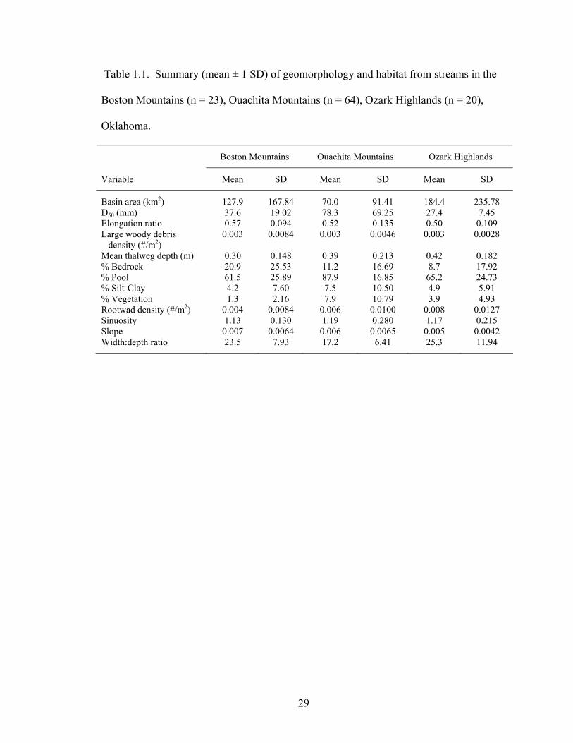
Table 1.1. Summary (mean ± 1 SD) of geomorphology and habitat from streams in the

Boston Mountains (n = 23), Ouachita Mountains (n = 64), Ozark Highlands (n = 20),

Oklahoma.

Boston Mountains Ouachita Mountains Ozark Highlands

Variable Mean SD Mean SD Mean SD

Basin area (km2) 127.9 167.84 70.0 91.41 184.4 235.78 D50 (mm) 37.6 19.02 78.3 69.25 27.4 7.45 Elongation ratio 0.57 0.094 0.52 0.135 0.50 0.109 Large woody debris density (#/m2)

0.003 0.0084 0.003 0.0046 0.003 0.0028

Mean thalweg depth (m) 0.30 0.148 0.39 0.213 0.42 0.182 % Bedrock 20.9 25.53 11.2 16.69 8.7 17.92 % Pool 61.5 25.89 87.9 16.85 65.2 24.73 % Silt-Clay 4.2 7.60 7.5 10.50 4.9 5.91 % Vegetation 1.3 2.16 7.9 10.79 3.9 4.93 Rootwad density (#/m2) 0.004 0.0084 0.006 0.0100 0.008 0.0127 Sinuosity 1.13 0.130 1.19 0.280 1.17 0.215 Slope 0.007 0.0064 0.006 0.0065 0.005 0.0042 Width:depth ratio 23.5 7.93 17.2 6.41 25.3 11.94

29

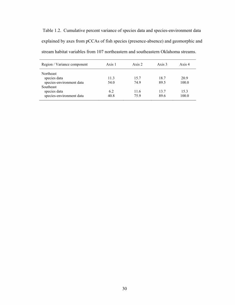
Table 1.2. Cumulative percent variance of species data and species-environment data

explained by axes from pCCAs of fish species (presence-absence) and geomorphic and

stream habitat variables from 107 northeastern and southeastern Oklahoma streams.

Region / Variance component Axis 1 Axis 2 Axis 3 Axis 4

Northeast species data 11.3 15.7 18.7 20.9 species-environment data 54.0 74.9 89.5 100.0 Southeast species data 6.2 11.6 13.7 15.3 species-environment data 40.8 75.9 89.6 100.0

30

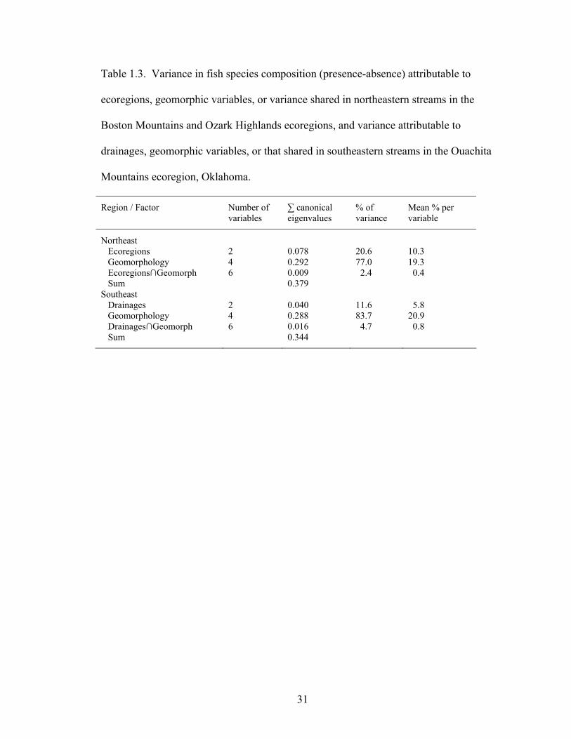
Table 1.3. Variance in fish species composition (presence-absence) attributable to

ecoregions, geomorphic variables, or variance shared in northeastern streams in the

Boston Mountains and Ozark Highlands ecoregions, and variance attributable to

drainages, geomorphic variables, or that shared in southeastern streams in the Ouachita

Mountains ecoregion, Oklahoma.

Region / Factor Number of variables

∑ canonical eigenvalues

% of variance

Mean % per variable

Northeast Ecoregions 2 0.078 20.6 10.3 Geomorphology 4 0.292 77.0 19.3 Ecoregions∩Geomorph 6 0.009 2.4 0.4 Sum 0.379 Southeast Drainages 2 0.040 11.6 5.8 Geomorphology 4 0.288 83.7 20.9 Drainages∩Geomorph 6 0.016 4.7 0.8 Sum 0.344

31

Fig. 1.1. Locations of 175 randomly selected stream sites used for an inventory of fluvial

geomorphology, stream habitat, and stream fishes in eastern Oklahoma, of which

completed species lists were collected at 107.

Fig. 1.2. pCCA biplots of fish species (A) and samples (B) and basin area, reach slope,

channel width:depth ratio, and median particle size (D50) summarizing differences in fish

species composition along longitudinal and local geomorphic gradients in Boston

Mountains (▲) and Ozark Highlands (□) streams. Species having weights greater than

5% are displayed. Species codes represent the first two letters of genus and first six of

species.

Fig. 1.3. pCCA biplots of fish species and basin area, reach slope, median particle size

(D50), and percent silt-clay summarizing differences in fish species composition along

longitudinal and local geomorphic gradients in Ouachita Mountains streams. Species

having weights greater than 5% are displayed. Species codes represent the first two

letters of genus and first six of species.

32

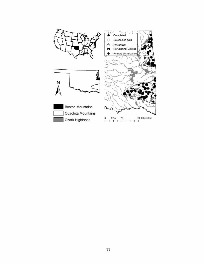
33

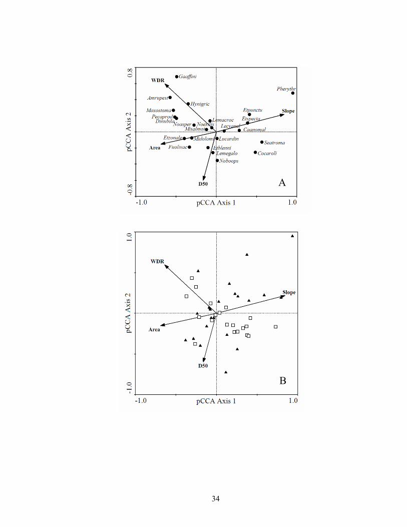
A

B

34

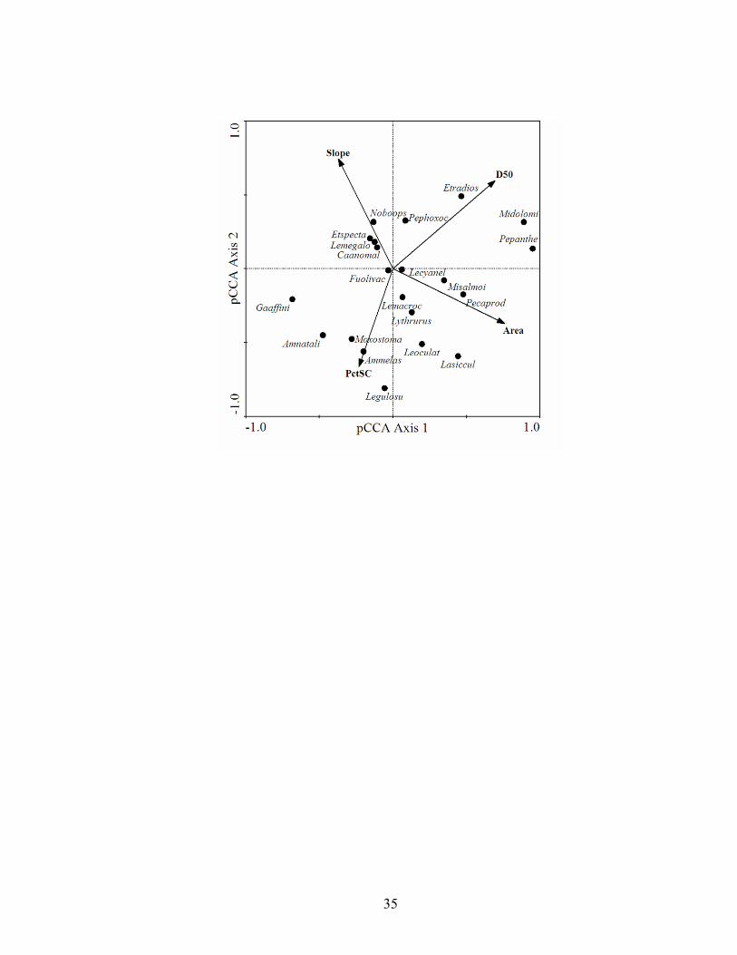
35

Appendix 1.1. Fish species by Boston Mountains (BM), Ouachita Mountains (OM), and

Ozark Highlands (OH) ecoregions observed during snorkeling surveys of eastern

Oklahoma streams. Nomenclature adopted from Miller and Robison (2004).

Family / Species Common Name BM OM OH

Petromyzontidae Ichthyomyzon spp. lampreys x x Lepisosteidae Lepisosteus oculatus Winchell spotted gar x x x Lepisosteus osseus (Linnaeus) longnose gar x x Clupeidae Dorosoma cepedianum (Lesueur) gizzard shad x x Cyprinidae Campostoma anomalum (Rafinesque) central stoneroller x x x Cyprinella lutrensis (Baird and Girard) red shiner x Cyprinella whipplei Girard steelcolor shiner x x x Cyprinus carpio Linnaeus common carp x x Dionda nubila (Forbes) Ozark minnow x x Luxilus cardinalis (Mayden) cardinal shiner x x Lythrurus spp. lythrurus shiners x Nocomis asper Lachner and Jenkins redspot chub x x Notropis boops Gilbert bigeye shiner x x x Phoxinus erythrogaster (Rafinesque) southern redbelly dace x x Pimephales notatus (Rafinesque) bluntnose minnow x x Semotilus atromaculatus (Mitchell) creek chub x x Catostomidae Catostomus commersoni (Lacépède) white sucker x x x Ictiobus spp. buffalos x Hypentelium nigricans (Lesueur) northern hogsucker x x Minytrema melanops (Rafinesque) spotted sucker x Moxostoma spp. redhorses x x x Ictaluridae Ameiurus melas (Rafinesque) black bullhead x x Ameiurus natalis (Lesueur) yellow bullhead x x x Ictalurus punctatus (Rafinesque) channel catfish x Noturus exilis Nelson slender madtom x x x Noturus nocturnus Jordan and Gilbert freckled madtom x Pylodictis olivaris Rafinesque flathead catfish x Esocidae Esox americanus Gmelin redfin pickerel x Salmonidae Oncorhynchus mykiss (Walbaum) rainbow trout x Aphredoderidae Aphredoderus sayanus (Gilliams) pirate perch x Fundulidae Fundulus catenatus (Storer) northern studfish x Fundulus olivaceus (Storer) blackspotted topminnow x x x Poeciliidae Gambusia affinis (Baird and Girard) western mosquitofish x x x Atherinopsidae Labidesthes sicculus (Cope) brook silverside x x

36

Cottidae Cottus carolinae (Gill) banded sculpin x x Centrarchidae Ambloplites rupestris (Rafinesque) rock bass x x Lepomis cyanellus Rafinesque green sunfish x x x Lepomis gulosus (Cuvier) warmouth x Lepomis humilis (Girard) orangespotted sunfish x Lepomis macrochirus Rafinesque bluegill x x x Lepomis megalotis (Rafinesque) longear sunfish x x x Lepomis microlophus (Gunther) redear sunfish x x x Micropterus dolomieu Lacepede smallmouth bass x x x Micropterus salmoides1 (Lacepede) largemouth bass x x x Pomoxis annularis Rafinesque white crappie x x x Pomoxis nigromaculatus (Lesueur) black crappie x Percidae Etheostoma blennioides Rafinesque greenside darter x x x Etheostoma flabellare Rafinesque fantail darter x x Etheostoma punctulatum (Agassiz) stippled darter x x Etheostoma radiosum (Hubbs and Black) orangebelly darter x Etheostoma spectabile (Agassiz) orangethroat darter x x x Etheostoma whipplei (Girard) redfin darter x Etheostoma zonale (Cope) banded darter x x Percina caprodes (Rafinesque) logperch x x x Percina copelandi (Jordan) channel darter x Percina maculata (Girard) blackside darter x Percina pantherina (Moore and Reeves) leopard darter x Percina phoxocephala (Nelson) slenderhead darter x Sciaenidae Aplodinotus grunniens (Rafinesque) freshwater drum x 1 included spotted bass Micropterus punctulatus

37

CHAPTER 2

GEOMORPHOLOGY AND STREAM HABITAT RELATIONSHIPS WITH

SMALLMOUTH BASS ABUNDANCE AT MULTIPLE SPATIAL SCALES IN

EASTERN OKLAHOMA

38

Abstract

Fluvial geomorphic processes play a major role in structuring habitats that are important

to stream fishes. We determined relationships between densities of smallmouth bass

(Micropterus dolomieu) and ecoregions, basin and reach geomorphology, and stream

habitat in the Boston Mountains, Ouachita Mountains, and Ozark Highlands ecoregions

of eastern Oklahoma. One hundred seventy-five stream sites were randomly selected;

sites were allocated in proportion to ecoregion areas and equally distributed among

stream orders 1 to 4. Geomorphology was measured at the basin and reach scales at 128

stream sites, and stream habitat and smallmouth bass abundance was measured in 1788

channel units. Some sites were inaccessible, dry, or had a primary disturbance (e.g.,

gravel mining) and were not sampled. Variation in geomorphology and stream habitat at

the basin and reach scales was related to stream size, channel morphology, and substrate

size. Channel morphology differed among ecoregions in the largest streams. Channel

units were typically riffles, runs, mid-channel pools, and backwaters. Habitat

characteristics varied widely among channel unit types and ecoregions. Densities of age-

0 and age-1+ smallmouth bass were approximately an order of magnitude greater in the

Boston Mountains and Ozark Highlands than in the Ouachita Mountains. Regression tree

analysis explained less variation in age-0 (10-fold cross-validated relative error = 0.844)

than age-1+ (relative error = 0.637) smallmouth bass densities, and showed that stream

size and channel-unit size were primary determinants of density. However, stream

morphology and channel-unit habitat were important in explaining additional variation in

densities somewhat independent of ecoregion. Understanding of geomorphic and stream

habitat influences on smallmouth bass abundance at multiple, nested spatial scales is

39

imperative for the management, conservation and restoration of smallmouth bass

populations.

40

Introduction

Fluvial geomorphology governs fluvial hydraulics and the physical habitat in streams

required by fishes (Yang 1971; Beschta and Platts 1986; Newson and Newson 2000).

Longitudinal processes reflecting basin characteristics, especially stream size, have been

shown to influence stream processes and biota (Vannote et al. 1980), but spatial

variability in geomorphic processes, controls, and disturbances within and among basins

and regions can affect local geomorphology and stream habitat within the longitudinal

continuum (Montgomery 1999; Benda et al. 2004).

Geomorphology affects stream biota at different organismal and organizational

levels. It has been shown to determine the distribution of stream habitat, ultimately

influencing macroinvertebrate community function and production in Appalachian

streams (Huryn and Wallace 1987). Geomorphology also influences the location of bull

trout (Salvelinus confluentus) redds (Baxter and Hauer 2000), influences essential sport-

fish habitat (Rabeni and Jacobson 1993), and structures stream fish assemblages (Walters

et al. 2003; Rhoads et al. 2003). Although geomorphic processes acting on specific

spatial scales have been implicated in affecting stream habitat and biota, connecting

geomorphology to physical habitat and biota in streams often requires incorporation of

processes at multiple spatial scales (Frissell et al. 1986; Newson and Newson 2000;

Frothingham et al. 2002).

Many stream habitat enhancement and restoration principles are geomorphically

based. Rosgen (1994; 1996) developed a stream classification system to determine, in

part, the potential for enhancement of fish habitat and river restoration. He suggested that

41

installation of instream structures intended as fish habitat may result in detrimental

channel adjustments and create disequilibrium stream conditions, and that only streams

exhibiting certain morphologic and sediment characteristics should be candidates for

habitat improvement structures. Rosgen also suggested that restoration principles should

incorporate the natural stable tendencies of a river that result from the interaction of

morphological variables. Champoux et al. (2003) found that long-term success of

instream structures was related to different glacial deposits (moraine versus outwash

plain), and argued that reach geomorphology needed to be considered during restoration

planning to ensure long-term effectiveness of habitat improvement structures and

management actions.

Eastern Oklahoma has several distinct regions. These ecoregions have

characteristic climate, landform, land use, vegetation, and soils (Omernik 1987; Woods et

al. 2005). There are also regional differences in fish assemblages and sport-fish

populations (Stark and Zale 1991; Balkenbush and Fisher 2001; Howell 2001; Tejan

2004); similarities among stream habitat and fish assemblages have been shown for the

same ecoregions in Arkansas (Rohm et al. 1987). Although seven ecoregions have been

delineated in eastern Oklahoma, Fisher et al. (2004) used ecoregion characteristics to

identify three fishery management regions: northeast, east-central, and southeast. They

showed that these management regions had distinct patterns of species richness and

population abundance, and the regions were developed to enhance the future management

of stream fisheries.

Although regional differences have been identified, it is unknown whether

observed patterns in these fisheries are reflective of regional scale characteristics or basin

42

and local scale geomorphic processes that may or may not be associated with those

regions. Our goal was to determine how longitudinal and local geomorphic processes

influenced smallmouth bass (Micropterus dolomieu) abundance in streams of the Boston

Mountains, Ouachita Mountains, and Ozark Highlands ecoregions in eastern Oklahoma.

These ecoregions harbor most of the native distribution of smallmouth bass in Oklahoma.

Relations among geomorphology, habitat, and smallmouth bass abundance will help

guide conservation, management, and enhancement of stream habitats formed by

geomorphic processes and used by smallmouth bass.

Study area

Relations between fluvial geomorphology and stream habitat, and smallmouth bass were

determined for small streams to mid-sized rivers in the Boston Mountains, Ouachita

Mountains, and Ozark Highlands level III ecoregions in eastern Oklahoma (Omernik

1987). The Boston Mountains ecoregion is a dissected mountainous plateau composed of

flat-lying shale and sandstone lithology and oak-hickory forest. Annual rainfall is 112 to

130 cm and land is used is mostly for logging and recreation (Woods et al. 2005). The

Ouachita Mountains consist of folded, Paleozoic sandstone, shale, and chert. Oak-

hickory-shortleaf pine forests in this region receive from 109 to 145 cm of annual

rainfall. Common land uses are: logging, pastureland, hayfields, farming, and recreation

(Rutherford et al. 1992; Woods et al. 2005). The Ozark Highlands are dominated by flat-

lying cherty limestone, but shale, limestone, and dolomite are present in valley bottoms.

Annual precipitation is 104 to 124 cm, and land use is primarily logging, recreation, and

43

cattle and poultry farming, including pastureland and hayfields (Rabeni and Jacobson

1993; Woods et al. 2005).

Methods

Stream survey

A geographic information system (GIS) was used as an aid in the random

selection of 175 stream sites for an inventory of fluvial geomorphology, stream habitat,

and smallmouth bass populations in the study area. To select stream sites, a stream

network was generated in a GIS using a 30 m digital elevation model (DEM) from the

National Elevation Dataset (USGS 1999). The network was then created by identifying

all cells in the DEM with a watershed size ≥ 1.35 km2, and defining them as a stream.

Stream orders (Strahler 1957) were assigned to each stream segment in the network.

One-hundred seventy-five sample sites were randomly selected on regional streams; they

were allocated to the three ecoregions approximately in proportion to ecoregion area, and

they were equally distributed among stream orders 1 to 4 in each ecoregion to ensure that

larger streams were represented. Forty sites each were selected in the Boston Mountains

and Ozark Highlands ecoregions, and 95 were selected in the Ouachita Mountains

ecoregion within Oklahoma. The GIS layer of sample sites was uploaded into a global

positioning (GPS) receiver that was used to navigate to each site. Streams were sampled

from mid-May to mid-August, 2003 to 2005, during low streamflow conditions.

44

Watershed and reach geomorphology and habitat

Watershed scale geomorphic variables for each site were derived using a GIS.

The aforementioned DEM was used to delineate drainage basins, and GIS was then used

to measure basin areas and lengths. Elongation ratio was measured as the diameter of a

circle with the same area as the basin divided by basin length (Morisawa 1968).

We measured fluvial geomorphic variables at each stream site. The stream reach

at each site was defined as 20 times the mean channel width (i.e., bankfull width)

upstream of each sample point; bankfull stage was identified by using visual and physical

indicators (Rosgen 1996). Channel units in each reach were classified using the scheme

of Hawkins et al. (1993). Transects perpendicular to the channel were surveyed across

two riffles and two pools when available, with a maximum of two transects in a single

channel unit; two to four transects were surveyed per reach. Entrenchment ratio,

width:depth ratio, and median particle size (i.e., D50) were calculated for each transect.

Entrenchment ratio was calculated as the ratio of floodprone width to bankfull channel

width. Floodprone elevation was equal to twice the maximum channel depth, and

floodprone width was estimated as the valley floor width at the floodprone elevation.

Maximum floodprone width was measured if it was less than 2.2 times the channel width

at each transect, otherwise it was recorded as 2.2. Width:depth ratio was calculated as the

ratio of bankfull channel width to mean bankfull channel depth. Channel depths were

measured at 20 equally-spaced locations along transects. Median particle size of surficial

substrates was calculated by collecting 100 particles along each transect and measuring

the intermediate axis of each; bedrock was excluded from analysis. Water surface slope

of each reach was measured. Sinuosity was measured as the ratio of stream length to

45

straight-line distance as measured on maps of the stream reach created with a GPS (see

below). Width:depth ratio and median particle size for the reach were calculated from

transect data as weighted averages based on the proportion of each reach length that

comprised riffles and pools (Zar 1999). Reach entrenchment ratios were calculated as the

median of transect values.

Channel-unit habitat

Stream habitat was measured in each channel unit within each reach using

methods conducive to a large-scale stream survey. Channel units were mapped with a

GPS, and lengths and areas of channel units were measured in a GIS (Dauwalter et al.

2006). Thalweg depths were measured multiple times per channel unit at equally spaced

intervals; more measurements were made in longer and more heterogeneous channel

units. A modified Wentworth scale was used to visually estimate substrate distributions

within each channel unit (Bain 1999). We estimated, and enumerated when logistically

feasible, boulders, rootwads, and large woody debris (10+ cm diameter, 4+ m in length)

in each channel unit. Percent undercut bank and percent vegetative coverage were also

estimated. Water velocity was coded by channel unit type as: falls = 4, riffle = 3, run = 2,

all other types = 1. Habitat variables for each channel unit were combined for reach

habitat estimates.

Smallmouth bass abundance

Smallmouth bass abundance was estimated by snorkeling or electrofishing

individual channel units within reaches (Dolloff et al. 1996; Reynolds et al. 1996). When

46

snorkeling, 1 to 3 person snorkel teams moved upstream in a zig-zag pattern and counted

and estimated sizes of smallmouth bass individuals. One electrofishing pass was made

using a backpack, barge, or boat electrofisher when water clarity prohibited effective

snorkeling (i.e., < 1 m). Water clarity was measured as the maximum distance at which a

snorkeler could see a 100 mm model of a smallmouth bass. Electrofishing power density

was standardized at approximately 1000 µS·cm-3 (Reynolds 1996; Miranda and Dolan

2003); however, settings on the backpack electrofisher prohibited obtaining 1000 µS·cm-3

exactly. Counted individuals were placed into <100 and ≥100 mm size categories.

Individuals <100 mm represent age-0 individuals and those ≥100 mm are age-1+

(Balkenbush and Fisher 2001); ages will be referred to hereafter. Snorkeling counts of

smallmouth bass were adjusted using a model comparing snorkeling counts to abundance

estimates, and electrofishing counts were adjusted using a 1-pass capture probability

model (Appendix 2.A).

Data analysis

We used a principle components analysis (PCA) to determine relationships among

variables at the basin and reach scales and to eliminate redundant covariables. The PCA

was conducted on the correlation matrix, and eigenvalues greater than those predicted

under the broken stick model were considered meaningful (Jackson 1993; McGarigal et

al. 2000). The predicted eigenvalue (b) for the kth component under the broken stick

model was calculated as: ∑==

kb

correlations were used to examine relationships among channel unit variables; the limited

p

ki i1 , where p was the number of variables. Pearson

47

number of variables precluded use of PCA at the channel unit spatial scale. Analyses

were run using SAS Version 9.1 software (SAS Institute Inc., Cary, North Carolina).

We used regression tree analysis (RTA) to determine the influence of ecoregions,

geomorphology, and stream habitat at the reach and channel unit spatial scales on the

density of smallmouth bass. RTA is a flexible and robust nonparametric method used to

assess complex relationships between explanatory variables and a response variable that

may be non-linear with high order interactions. It explains variation in the response

variable by splitting the dataset into homogenous groups using specific values of the

categorical or continuous explanatory variables. Groups include observations that have

common values of explanatory and response variables. Regression trees are displayed

graphically for ease of interpretation (Breiman et al. 1984; De'ath and Fabricius 2000).

RTA has been used in other ecological studies of complex relationships between

explanatory and response variables when common linear modeling approaches have

failed (Rejwan et al. 1999; De'ath and Fabricius 2000).

We conducted RTA for data collected at the ecoregion, basin and reach, and

channel-unit scales in one analysis for each age group. Explanatory variables included in

RTA were dependent on results of PCA and correlation analyses to limit variable

redundancy. Smallmouth bass densities (no.·ha-1) were transformed (loge[X + 0.01]) to

reduce the effects of zero densities on variances. Each RTA was performed with CART

version 5.0 software (Steinberg and Colla 1995). We used sums of squares about the

group means as the measure to maximize homogeneity within groups; sums of absolute

deviations about the median is more robust, but can be ineffective when many zeros are

present (De'ath and Fabricius 2000). The final tree selected was the one with the smallest

48

relative error (similar to the coefficient of nondetermination, 1 – r2) based on 10-fold

cross-validation (Breiman et al. 1984; De'ath and Fabricius 2000).

Results

Stream survey

We surveyed channel geomorphology, stream habitat, and smallmouth bass

abundance at 128 of 175 selected stream sites. Seventeen stream sites were either

inaccessible or access was denied by landowners. Direct channel alteration by humans

(e.g., gravel mining) was observed at five stream sites, and these sites were not sampled.

Twenty-two streams were dry. Two sites were not snorkeled, and habitat measurements

were incomplete at another. Complete information on geomorphology, stream habitat,

and smallmouth bass abundance was collected at 128 stream sites (Figure 2.1);

electrofishing was conducted at 17 sites in the Ouachita Mountains. Among all sites,

1788 channel units were sampled.

Watershed and reach geomorphology and habitat

Geomorphology and stream habitat were more similar at the basin and reach

scales in the Boston Mountains and Ozark Highlands than in the Ouachita Mountains

(Table 2.1). Ouachita Mountains streams had smaller basin sizes on average, likely

because most small streams in the other ecoregions were dry and excluded from analyses.

These streams generally had higher reach slopes and particle sizes and more vegetation,

silt-clay substrate, and pool area. They were also typically deeper, had less wood, and

lower width:depth ratios than streams in the other regions. Stream reaches in the Boston

49

Mountains were typically shallower and had more bedrock. Ozark Highland streams

were generally deeper with more wood, wider channels, smaller particle sizes, and less

bedrock on average when compared to streams in the other two regions. Variability in

geomorphology and stream habitat was often greater in the Ouachita Mountains, the

largest ecoregion.

At the basin and reach scales, PCA revealed two informative principle

components according to the broken stick criterion; however, the third principle

component also appeared important (Table 2.2). Axis 1 reflected stream size, with high

loadings for basin area, reach slope, and mean thalweg depth. Axis 2 reflected channel

morphology. Width:depth ratio loaded most heavily on axis 2, but percent silt-clay also

had a high loading followed by percent pool and percent bedrock. Axis 3 represented a

particle size axis, dominated by D50 and followed by percent pool and sinuosity. PCA

biplots showed that channel morphology (axis 2) in the largest streams differed between

the Ozark Highlands and Ouachita Mountains ecoregions (axis 1; far right of Figure 2.2).

Channel-unit habitat

We observed 11 channel unit types in all. Riffles, runs, and mid-channel pools

were the most abundant types in each ecoregion. Habitat characteristics were highly

variable among channel unit types and ecoregions (Table 2.3). No variables among the

1788 channel units were highly correlated (Table 2.4). Velocity and mean thalweg depth

had the highest Pearson correlation at r = -0.398.

50

Smallmouth bass abundance

Smallmouth bass densities varied widely, but were typically higher in the Boston

Mountains and Ozark Highlands. No smallmouth bass were collected in stream reaches

that were electrofished. Density estimates of age-0 smallmouth bass in channel units

ranged from 0·ha-1in all ecoregions to 1,492·ha-1 in the Boston Mountains, 770·ha-1 in the

Ouachita Mountains, and 629·ha-1 in the Ozark Highlands. Densities of age-1+

smallmouth bass ranged from 0·ha-1 in all ecoregions, to 2,010·ha-1 in the Boston

Mountains, 381·ha-1 in the Ouachita Mountains, and 1,217·ha-1 in the Ozark Highlands.

Densities were consistently high in runs and pools, although some riffles, abandoned

channels, and backwaters also had high densities (Table 2.5).

Stream size, channel unit depth, and reach geomorphology variables explained

variation in densities of age-0 smallmouth bass. Seven basin-reach and seven channel-

unit scale variables were included in RTAs. Although reach slope was correlated with

basin area, we retained both because of variability observed in the Ouachita Mountains

ecoregion. Rootwad and large woody debris densities were combined (added) to form a

wood density variable. Elongation ratio was not included because of the lack of direct

biological influence on fish abundance. The regression tree with the minimum cross-

validated relative error, 0.825, had 17 nodes, 9 that were terminal. Densities were higher

in deeper channel units in larger streams, and were dependent on reach morphology

(Figure 2.3).

Several basin-reach and channel-unit variables explained most of the variation in

densities of age-1+ smallmouth bass. Variables included in the RTA were the same as

those for age-0 smallmouth bass. The regression tree with the minimum cross-validated

51

relative error, 0.627, had 24 splitting nodes and 25 terminal nodes. Shallow channel

units, regardless of stream size had the lowest densities, followed by deeper channel units

in small streams. However, high densities were also observed in some channel units of

small streams having unique reach and channel unit characteristics. Densities in deeper

channel units of small and large streams were higher, but dependent on reach

geomorphology and channel unit habitat specific to stream size (Figure 2.4).

Discussion

Our survey of 128 randomly selected stream reaches revealed that geomorphic

and habitat characteristics of streams at different spatial scales were differentially related

to densities of age-0 and age-1+ smallmouth bass. Densities of age-0 and age-1+

smallmouth bass were primarily explained by measures of stream and channel-unit size.

Although basin area was used as the surrogate measure of stream size, water-surface

slope and mean thalweg depth in the reach were negatively and positively related,

respectively, to basin area. Stream size likely influenced suitable nesting habitat and fry

production by smallmouth bass. Orth and Newcomb (2002) suggested that stochastic

streamflows and poor reproductive habitat limit smallmouth bass reproduction in small

streams; streamflow variability and unpredictability is typically greater in small streams

(Poff and Ward 1989). Some populations have individuals that migrate into tributaries in

spring to spawn, but they return to larger rivers after spawning (Lyons and Kanehl 2002).

In addition, many small streams in the Ozark Highlands region become intermittent or

dry. Smallmouth bass densities did not decrease in the largest streams we sampled. This

reflected our sampling design. Had we sampled larger streams (e.g., > fourth order), we

52

likely would have observed decreased densities or absence of smallmouth bass, as shown

by Tejan (2004) and suggested by Stark and Zale (1991). Rabeni and Jacobson (1993)

suggested that smallmouth bass densities decrease with increased valley width due to

finer bedload materials and less stream contact with valley walls resulting in a lower

number of bluff pools that are important smallmouth bass habitats. Thus, intermediate-

sized streams and rivers in eastern Oklahoma likely provide the streamflow and habitat

conditions most suitable for smallmouth bass populations.

Water depth has previously been shown to be important for determining

smallmouth bass abundance. Shallow channel units typically had zero or low densities

regardless of stream size. Smallmouth bass typically do not use depths less than about

0.25 m regardless of size (Todd and Rabeni 1989; Orth and Newcomb 2002). Avoidance

of shallow water may be a behavioral adaptation to circumvent predation by terrestrial

vertebrates. As noted above, small streams are likely reproduction limited, so even deep

channel units in small streams will have few if any smallmouth bass. Regression tree

analyses showed that deeper channel units in larger streams had higher densities;

however, microhabitat studies have shown that the deepest areas of channel units are used

less (Orth and Newcomb 2002). This may reflect the proximity of cover to stream banks

away from deep areas near the thalweg, but smallmouth bass may still select channel

units with deeper areas that can be used as escape cover.

Beyond the observed stream and channel unit-size effects, reach morphology

explained some additional variation in smallmouth bass densities. We found that stream

reaches with intermediate to high width:depth ratios (26-31) had channel units that

supported the highest fish densities. Width:depth ratio typically reflects channel stability

53

and percent silt-clay in the channel perimeter and banks (both negatively related), and is

positively related to discharge and sediment loads; sinuosity also reflects silt-clay content

of banks and typically varies inversely with width:depth ratio (Knighton 1998). In the

Ozark Highlands, accelerated erosion due to logging and overgrazing has likely increased

runoff and bedload dynamics, resulting in wider, gravel-dominated channels (Rabeni and

Jacobson 1993). This may have affected historical smallmouth bass production, as gravel

is required spawning substrates for smallmouth bass (Pflieger 1966), and may be why

age-0 densities were higher in reaches with high width:depth ratios. Increased channel

widths also result in less canopy cover per stream width and increased production of

stream invertebrates beneficial to fishes, such as juvenile smallmouth bass (Livingstone

and Rabeni 1991), as long as the increased sediment load is primarily gravel and not fines

(Waters 1995).

Other studies in Ozark streams have suggested that channel instability and

widening are detrimental to smallmouth bass. In northern Arkansas, gravel mining led to

wider channels and larger pools, and resulted in decreased abundances of smallmouth

bass (Brown et al. 1998). We did not sample streams with extreme width:depth ratios

resulting from anthropogenic activities, because we did not sample physically disturbed

stream sites, such as those with signs of gravel extraction. This may explain why we

observed increases in density with higher width:depth ratios. Sowa and Rabeni (1995)

found maximum summer water-temperature to be negatively related to smallmouth bass

densities but positively related to largemouth bass densities (M. salmoides) in Missouri

streams. They suggested that thermal inputs from reduced canopy cover and wider

channels increased water temperatures. We did not measure water temperatures, but they

54

are typically cooler and less variable in Boston Mountains and Ozark Highlands streams

(Robel 1996; Balkenbush and Fisher 2001) and likely increase with stream size (Allan

1995). Warmer temperatures (above 22°C) limit the growth scope of age-1+ smallmouth

bass and lead to a potential competitive advantage for largemouth bass (Zweifel et al.

1999; Whitledge et al. 2002). This may be why smallmouth bass mortality is higher

(Balkenbush and Fisher 2001) and densities lower in Ouachita Mountains streams

compared to northeastern streams. Thus, the relation between smallmouth bass density

and width:depth ratio is expected to be unimodal whereby intermediate width:depth ratios

support the highest densities of smallmouth bass, but confirmation of this relationship in

eastern Oklahoma is needed.

We also found that reaches with more riffle-pool structure (less percent pool

overall) in larger streams had higher smallmouth bass densities. This is interesting

because smallmouth bass densities are higher in deep pool habitats. However, Sowa and

Rabeni (1995) reported that smallmouth bass densities were higher in Missouri streams

that had a smaller reach area represented as pool habitat. They suggested that low

velocity habitats, such as pools, have more fine substrates that would be detrimental to

food resources (crayfish) preferred by smallmouth bass. Crayfish production has been

reported to be higher in riffles than pools in larger streams (Roell and Orth 1992).

Consequently, as riffle:pool ratios decrease, such as in southeastern Oklahoma streams,

there is less crayfish production in riffles per unit of pool habitat, leading to reduced prey

availability to smallmouth bass. Although riffle:pool structure is influenced by

geomorphic processes, anthropogenic activities (e.g., gravel mining) can also lower

riffle:pool ratios and negatively impact smallmouth bass populations (Brown et al. 1998).

55

Spatial variability in geomorphic processes and disturbances in the landscape

produces reaches that are morphologically homogenous and appear as patches (sensu

Townsend 1989) in the longitudinal continuum of streams (Montgomery 1999). Some

researchers have argued that this often occurs at tributary junctions (Poole 2002; Benda et

al. 2004). We did not attempt to document abrupt changes and subsequent spatial

variability in geomorphic process or disturbance. But, because stream morphology

influences smallmouth bass populations and is often similar throughout a reach, the

degree to which this patch phenomena exists and what exactly causes it in eastern

Oklahoma streams needs further study.

Except for water depth, channel-unit variables were not related to age-0 densities

of smallmouth bass. Sabo and Orth (1994) found that, although age-0 smallmouth bass

transitioned to using shallower, higher velocity areas as they grew through the summer,

their use of microhabitats also became more generalized. Pert et al. (2002) suggested that

age-0 smallmouth bass may be habitat generalists among stream systems, but specialists

within a stream. This is because they can adapt to a range of stream environments but

use specific resources that are most beneficial to them within a system. Swimming

ability of age-0 individuals may also prohibit them from moving into desired channel

units, especially between pools separated by riffles. Consequently, densities of age-0

smallmouth bass in channel units may reflect the quality of spawning habitat (Cleary

1956), number of successful nests and nest production (Reynolds and O'Bara 1991;

Lukas and Orth 1995), and/or survival dynamics of fry and juveniles through their first

summer (Knotek and Orth 1998). Selection of specific channel units with certain habitat

56

characteristics may be less important, especially in reaches with high width:depth ratios

dominated by gravel substrates.

Channel-unit characteristics were related to age-1+ smallmouth bass densities, but

these relations changed depending on stream size and reach morphology. The presence

of bedrock in shallow channel units led to increased densities, likely because local bed

scour along bedrock outcroppings resulted in small, deep areas in otherwise shallow

channel units. Deeper channel-units in larger streams with high wood densities had low

densities of fish: wood may have been too dense for smallmouth bass to use effectively.

We also observed no density relations with boulders. At the reach scale, smallmouth bass

abundance was not related to wood or boulder densities in a study of 23 reaches (250-

500m) on 19 Missouri streams (Sowa and Rabeni 1995). McClendon and Rabeni (1987)

found that boulder abundance, but not wood abundance, was positively related to

smallmouth bass biomass and density at the channel unit scale in Jacks Fork River,

Missouri; however, smallmouth bass size structure (i.e., proportional stock density)

increased with wood abundance. Rabeni and Jacobson (1993) suggested that boulders

were important and were often associated with bluff pool habitats. In our study, channel

units with lower wood densities and a fraction of silt-clay substrate also had low

densities. Fine sediments represent unsuitable habitat for the benthic macroinvertebrates

and crayfishes consumed by smallmouth bass in these streams (Waters 1995; Pflieger

1996; Fenner et al. 2004). Smallmouth bass were less abundant or absent in stream

reaches with more fines in Wisconsin (Lyons 1991). In some instances, we observed that

channel units with vegetation also had lower densities. Use of vegetation can be

detrimental to age-0 smallmouth bass when compared to other habitats (Olson et al.

57

2003), but abundance of vegetation was unrelated to abundance of adult smallmouth bass

in Missouri streams (McClendon and Rabeni 1987).

Microhabitat studies have shown that smallmouth bass are associated with woody

debris (Probst et al. 1984; Todd and Rabeni 1989; Lobb and Orth 1991) and boulders

(Probst et al. 1984; Rankin 1986; Todd and Rabeni 1989), but these associations are often

weak or absent at the channel-unit and reach spatial scales. Relations between fish and

cover density are likely complicated because multiple individuals may use a single cover

structure (Probst et al. 1984; Todd and Rabeni 1989), or cover may only determine the

distribution of individuals within a channel unit or reach and not influence production

and population dynamics. Production and population dynamics are more likely to be

affected by larger scale phenomena such as geomorphology and/or regional factors that

may or may not be independent of geomorphology (e.g., water temperature, land use;

Rabeni and Sowa 1996).

Interestingly, ecoregion did not have a direct influence on smallmouth bass

density in regression tree analyses. Others have reported higher smallmouth bass

densities in northeastern (Boston Mountains and Ozark Highlands) than southeastern

(Ouachita Mountains) Oklahoma streams (Stark and Zale 1991; Balkenbush and Fisher

2001). We also found densities in northeastern streams to be higher. However, the

regional differences were more related to variation in reach morphology in larger streams

with high densities than they were to ecoregions. Reach morphology of large streams

was different between ecoregions, and reflects differences in lithology, sediment regimes,

land use, and hydrology among ecoregions (Woods et al. 2005). It also incorporates

differences in watershed and local processes that vary within ecoregions. Consequently,

58

reach morphology is more closely linked to stream habitats used by smallmouth bass than

are ecoregions.

The need to understand how physical characteristics of streams influence stream

fishes at multiple spatial scales is not a new concept (Frissell et al. 1986; Wiens 2002),

but essential for effective stream restoration. We observed strong stream-size effects, but

geomorphic influences on smallmouth bass were complex and different between small

and large streams. Rabeni and Sowa (1996) stressed the importance of realizing the

nestedness of spatial scales and understanding how factors acting on different spatial

scales are important to the conservation of stream fishes. Geomorphic processes are

naturally hierarchical, and understanding spatial variability associated with those

processes is important to understanding how they structure fish habitat in streams

(Montgomery 1999). Most often, large-scale processes influence stream morphology and

function at smaller spatial scales but local impacts do not always influence large-scale

processes. There are exceptions, as upstream and downstream channel adjustments may

occur from a localized disturbance. Consequently, many stream restoration and habitat

enhancement projects have a geomorphic basis that includes different spatial scales

(Rosgen 1996; FISRWG 1998; Montgomery and Bolton 2003). Thus, understanding

how smallmouth bass populations respond to geomorphic processes is essential in

realizing how certain conservation and management practices aimed at changing

geomorphology may influence fishing for popular sport fish (Fisher et al. 2002) and

affect indicator species (Hlass et al. 1998) in these upland regions of the central United

States.

59

Acknowledgments

We thank V. Horncastle, S. Davis, A. Krystyniak, B. Marston, R. Ary, K. Winters, M.

Murray, and J. Morel for field assistance. R. Marston, J. Bidwell, A. Echelle, and D.

Splinter reviewed manuscript drafts. Project funding was provided by a Federal Aid in

Sport Fish Restoration Act grant under Project F-55-R of the Oklahoma Department of

Wildlife Conservation and the Oklahoma Cooperative Fish and Wildlife Research Unit.

The Oklahoma Cooperative Fish and Wildlife Research Unit is jointly sponsored by the

U. S. Geological Survey; Oklahoma State University; the Oklahoma Department of

Wildlife Conservation; the Wildlife Management Institute; and the U. S. Fish and

Wildlife Service. D. Dauwalter was supported by a Fellowship for Water, Energy, & the

Environment from the Environmental Institute, Oklahoma State University.

References

Allan, J.D. 1995. Stream ecology: structure and function of running waters. Chapman &

Hall, New York, New York.

Bain, M.B. 1999. Substrate. In Aquatic habitat assessment: common methods. Edited by

M.B. Bain and N.J. Stevenson. American Fisheries Society, Bethesda, Maryland. pp.

95-103.

Balkenbush, P.E. and Fisher, W.L. 2001. Population characteristics and management of

black bass in eastern Oklahoma streams. Proc. Annu. Conf. SEAFWA 53: 130-143.

Baxter, C.V. and Hauer, F.R. 2000. Geomorphology, hyporheic exchange, and selection

of spawning habitat by bull trout (Salvelinus confluentus). Can. J. Fish. Aquat. Sci.

57: 1470-1481.

60

Benda, L., Poff, N.L., Miller, D., Dunne, T., Reeves, G., Pess, G., and Pollock, M. 2004.

The network dynamics hypothesis: how channel networks structure riverine habitat.

BioScience 54: 413-427.

Beschta, R.L. and Platts, W.S. 1986. Morphological features of small streams:

significance and function. Water Resour. Bull. 22: 370-379.

Breiman, L., Friedman, J., Olshen, R., and Stone, C. 1984. Classification and regression

trees. Wadsworth International Group, Belmont, California.

Brown, A.V., Lyttle, M.M., and Brown, K.B. 1998. Impacts of gravel mining on gravel

bed streams. Trans. Amer. Fish. Soc. 127: 979-994.

Champoux, O., Biron, P.M., and Roy, A.G. 2003. The long-term effectiveness of fish

habitat restoration practices: Lawrence Creek, Wisconsin. Ann. Assoc. Amer.

Geographers 93: 42-54.

Cleary, R.E. 1956. Observations on factors affecting smallmouth bass production in

Iowa. J. Wildl. Manage. 20: 353-359.

Dauwalter, D.C., Fisher, W.L., and Belt, K.C. 2006. Mapping stream habitats with a

global positioning system: accuracy, precision, and comparison with traditional

methods. Environ. Manag. 37: 271-280.

De'ath, G. and Fabricius, K.E. 2000. Classification and regression trees: a powerful yet

simple technique for ecological data analysis. Ecology 81: 3178-3192.

Dolloff, A., Kershner, J., and Thurow, R. 1996. Underwater observation. In Fisheries

techniques. Edited by B.R. Murphy and D.W. Willis. American Fisheries Society,

Bethesda, Maryland. pp. 533-554.

61

Fenner, D.B., Walsh, M.G., and Winkelman, D.L. 2004. Diet overlap of introduced

rainbow trout and three native fishes in an Ozark stream. Amer. Fish. Soc. Symp. 44:

475-482.

Fisher, W.L., Schreiner, D.F., Martin, C.D., Negash, Y.A., and Kessler, E. 2002.

Recreational fishing and socioeconomic characteristics of eastern Oklahoma stream

anglers. Proc. Okla. Acad. Sci. 82: 79-87.

Fisher, W.L., Tejan, E.C., and Balkenbush, P.E. 2004. Regionalization of stream fisheries

management using Geographic Information Systems. In Proceedings of the second

international symposium on GIS/spatial analyses in fishery and aquatic sciences.

Edited by T. Nishida, P.J. Kailola, and C.E. Hollingworth. Fishery-Aquatic GIS

Research Group, Kawagoe, Saitama, Japan. pp. 465-476.

FISRWG. 1998. Stream corridor restoration: principles, processes, and practices. The

Federal Interagency Stream Restoration Working Group (FISRWG)(15 federal

agencies of the US gov't). No. GPO item no. 0120; SuDocs no. 57.6/2:EN3/PT.653.

ISBN-0-934213-59-3.

Frissell, C.A., Liss, W.J., Warren, C.E., and Hurley, M.D. 1986. A hierarchical

framework for stream habitat classification: viewing streams in a watershed context.

Environ. Manag. 10: 199-214.

Frothingham, K.M., Rhoads, B.L., and Herricks, E.E. 2002. A multiscale conceptual

framework for integrated ecogeomorphological research to support stream

naturalization in the agricultural Midwest. Environ. Manag. 29: 16-33.

Hawkins, C.P. and others 1993. A hierarchical approach to classifying stream habitat

features. Fisheries 18(6): 3-12.

62

Hlass, L.J., Fisher, W.L., and Turton, D.J. 1998. Use of the Index of Biotic Integrity to

assess water quality in forested streams in the Ouachita Mountains ecoregion,

Arkansas. J. Freshw. Ecol. 13: 181-192.

Howell, C.E.Jr. 2001. Correspondence between aquatic ecoregions and the distribution of

fish communities of eastern Oklahoma. M.S. thesis, University of North Texas,

Denton, Texas.

Huryn, A.D. and Wallace, J.B. 1987. Local geomorphology as a determinant of

macrofaunal production in a mountain stream. Ecology 68: 1932-1942.

Jackson, D.A. 1993. Stopping rules in PCA: a comparison of heuristical and statistical

approaches. Ecology 74: 2205-2214.

Knighton, D. 1998. Fluvial forms and processes: a new perspective. Oxford University

Press, Inc., New York.

Knotek, W.L. and Orth, D.J. 1998. Survival for specific life intervals of smallmouth bass,

Micropterus dolomieu, during parental care. Env. Biol. Fish. 51: 285-296.

Livingstone, A.C. and Rabeni, C.F. 1991. Food-habitat relations of underyearling

smallmouth bass in an Ozark stream. In First international smallmouth bass

symposium. Edited by D.C. Jackson. Mississippi Agricultural and Forestry

Experiment Station, Mississippi State University, Mississippi State. pp. 76-83.

Lobb, M.D.I. and Orth, D.J. 1991. Habitat use by an assemblage of fish in a large

warmwater stream. Trans. Amer. Fish. Soc. 120: 65-78.

Lukas, J.A. and Orth, D.J. 1995. Factors affecting nesting success of smallmouth bass in

a regulated Virginia stream. Trans. Amer. Fish. Soc. 124: 726-735.

63

Lyons, J. 1991. Predicting smallmouth bass presence/absence and abundance in

Wisconsin streams using physical habitat characteristics. In The first international

smallmouth bass symposium. Edited by D.C. Jackson. Mississippi Agricultural and

Forestry Experiment Station, Mississippi State University, Mississippi State. pp. 96-

103.

Lyons, J. and Kanehl, P.D. 2002. Seasonal movements of smallmouth bass in streams. In

Black bass: ecology, conservation, and management. Edited by D.P. Philipp and M.S.

Ridgway. American Fisheries Society, Symposium 31, Bethesda, Maryland. pp. 149-

160.

McClendon, D.D. and Rabeni, C.F. 1987. Physical and biological variables useful for

predicting population characteristics of smallmouth bass and rock bass in an Ozark

stream. N. Am. J. Fish. Manage. 7: 46-56.

McGarigal, K., Cushman, S., and Stafford, S. 2000. Multivariate statistics for wildlife

and ecology research. Springer-Verlag, New York.

Miranda, L.E. and Dolan, C.R. 2003. Test of a power transfer model for standardizing

electrofishing. Trans. Amer. Fish. Soc. 132: 1179-1185.

Montgomery, D.R. 1999. Process domains and the river continuum. J. Am. Water

Resour. Assoc. 36: 397-410.

Montgomery, D.R. and Bolton, S.M. 2003. Hydrogeomorphic variability and river

restoration. In Strategies for restoring river ecosystems: sources of variability and

uncertainty in natural and managed systems. Edited by R.C. Wissmar and P.A.

Bisson. American Fisheries Society, Bethesda, Maryland. pp. 39-80.

64

Morisawa, M. 1968. Streams: their dynamics and morphology. McGraw-Hill Book

Company, New York.

Newson, M.D. and Newson, C.L. 2000. Geomorphology, ecology and river channel

habitat: mesoscale approaches to basin-scale challenges. Prog. Phys. Geog. 24: 195-

217.

Olson, M.H., Young, B.P., and Blinkoff, K.D. 2003. Mechanisms underlying habitat use

of juvenile largemouth bass and smallmouth bass. Trans. Amer. Fish. Soc. 132: 398-

405.

Omernik, J.M. 1987. Ecoregions of the conterminous United States. Ann. Assoc. Amer.

Geographers 77: 118-125.

Orth, D.J. and Newcomb, T.J. 2002. Certainties and uncertainties in defining essential

habitats for riverine smallmouth bass. In Black bass: ecology, conservation, and

management. Edited by D.P. Philipp and M.S. Ridgway. American Fisheries Society,

Symposium 31, Bethesda, Maryland. pp. 251-264.

Pert, E.J., Orth, D.J., and Sabo, M.J. 2002. Lotic-dwelling age-0 smallmouth bass as both

resource specialists and generalists: reconciling disparate literature reports. In Black

bass: ecology, conservation, and management. Edited by D.P. Philipp and M.S.

Ridgway. American Fisheries Society, Symposium 31, Bethesda, Maryland. pp. 185-

189.

Pflieger, W.L. 1966. Reproduction of the smallmouth bass (Micropterus dolomieui) in a

small Ozark stream. Amer. Midl. Nat. 76: 411-418.

Pflieger, W.L. 1996. The crayfishes of Missouri. Missouri Department of Conservation,

Jefferson City, Missouri.

65

Poff, N.L. and Ward, J.V. 1989. Implications of streamflow variability and predictability

for lotic community structure: a regional analysis of streamflow patterns. Can. J. Fish.

Aquat. Sci. 46: 1805-1818.

Poole, G.C. 2002. Fluvial landscape ecology: addressing uniqueness within the river

discontinuum. Freshwat. Biol. 47: 641-660.

Probst, W.E., Rabeni, C.F., Covington, W.G., and Marteney, R.E. 1984. Resource use by

stream-dwelling rock bass and smallmouth bass. Trans. Amer. Fish. Soc. 113: 283-

294.

Rabeni, C.F. and Jacobson, R.B. 1993. Geomorphic and hydraulic influences on the

abundance and distribution of stream centrarchids in Ozark USA streams. Pol. Arch.

Hydrobiol. 40: 87-99.

Rabeni, C.F. and Sowa, S.P. 1996. Integrating biological realism into habitat restoration

and conservation strategies for small streams. Can. J. Fish. Aquat. Sci. 53(Suppl. 1):

252-259.

Rankin, E.T. 1986. Habitat selection by smallmouth bass in response to physical

characteristics in a natural stream. Trans. Amer. Fish. Soc. 115: 322-334.

Rejwan, C., Collings, N.C., Brunner, L.J., Shuter, B.J., and Ridgway, M.S. 1999. Tree

regression analysis on the nesting habitat of smallmouth bass. Ecology 80: 341-348.

Reynolds, C.R. and O'Bara, C.J. 1991. Reproductive ecology and spawning habitat of

smallmouth bass in two small streams of the Tennessee River system. In The first

international smallmouth bass symposium. Edited by D.C. Jackson. Mississippi

Agricultural and Forestry Experiment Station, Mississippi State. pp. 61-65.

66

Reynolds, J.B. 1996. Electrofishing. In Fisheries techniques. Edited by B.R. Murphy and

D.W. Willis. American Fisheries Society, Bethesda, Maryland. pp. 221-253.

Rhoads, B.L., Schwartz, J.S., and Porter, S. 2003. Stream geomorphology, bank

vegetation, and three-dimensional habitat hydraulics for fish in midwestern

agricultural streams. Water Resour. Res. 39: 1218.

Robel, G.L. 1996. Bioenergetics of smallmouth bass Micropterus dolomieu in Oklahoma

hatcheries and streams. M.S. thesis, Oklahoma State University, Stillwater,

Oklahoma.

Roell, M.J. and Orth, D.J. 1992. Production of three crayfish populations in the New

River of West Virginia, USA. Hydrobiologia 228: 185-194.

Rohm, C.M., Giese, J.W., and Bennett, C.C. 1987. Evaluation of an aquatic ecoregion

classification of streams in Arkansas. J. Freshw. Ecol. 4: 127-141.

Rosgen, D.L. 1994. A classification of natural rivers. Catena 22: 169-199.

Rosgen, D.L. 1996. Applied river morphology. Wildland Hydrology, Pagosa Springs,

Colorado.

Rutherford, D.A., Echelle, A.A., and Maughan, O.E. 1992. Drainage-wide effects of

timber harvesting on the structure of stream fish assemblages in southeastern

Oklahoma. Trans. Amer. Fish. Soc. 121: 716-728.

Sabo, M.J. and Orth, D.J. 1994. Temporal variation in microhabitat use by age-0

smallmouth bass in the North Anna River, Virginia. Trans. Amer. Fish. Soc. 123:

733-746.

67

Sowa, S.P. and Rabeni, C.F. 1995. Regional evaluation of the relation of habitat to

distribution and abundance of smallmouth bass and largemouth bass in Missouri

streams. Trans. Amer. Fish. Soc. 124: 240-251.

Stark, W.J. and Zale, A.V. 1991. Status of smallmouth bass populations in eastern

Oklahoma. Federal Aide Project, Oklahoma Department of Wildlife Conservation,

Oklahoma City. No. F-41-R.

Steinberg, D. and Colla, P. 1995. CART: Tree-structured non-parametric data analysis.

Salford Systems, San Diego, California.

Strahler, A.N. 1957. Quantitative analysis of watershed geomorphology. Trans. Am. Geo.

Union 38: 913-920.

Tejan, E. 2004. Landscape-scale influences on stream fish assemblages in eastern

Oklahoma. M.S. thesis, Oklahoma State University, Stillwater, Oklahoma.

Todd, B.L. and Rabeni, C.F. 1989. Movement and habitat use by stream-dwelling

smallmouth bass. Trans. Amer. Fish. Soc. 118: 229-242.

Townsend, C.R. 1989. The patch dynamics concept of stream community ecology. J. N.

Am. Benthol. Soc. 8: 36-50.

USGS. 1999. National elevation dataset, 1st ed. U.S. Geological Survey, Sioux Falls.

Vannote, R.L., Minshall, G.W., Cummins, K.W., and Cushing, C.E. 1980. The river

continuum concept. Can. J. Fish. Aquat. Sci. 37: 130-137.

Walters, D.M., Leigh, D.S., Freeman, M.C., Freeman, B.J., and Pringle, C.M. 2003.

Geomorphology and fish assemblages in a Piedmont river basin, U.S.A. Freshwat.

Biol. 48: 1950-1970.

68

Waters, T.F. 1995. Sediment in streams: sources, biological effects, and control.

American Fisheries Society Monograph 7, Bethesda, Maryland.

Whitledge, G.W., Hayward, R.S., and Rabeni, C.F. 2002. Effects of temperature on

specific daily metabolic demand and growth scope of sub-adult and adult smallmouth

bass. J. Freshw. Ecol. 17: 353-361.

Wiens, J.A. 2002. Riverine landscapes: taking landscape ecology into the water.

Freshwat. Biol. 47: 501-515.

Woods, A.J., Omernik, J.M., Butler, D.R., Ford, J.G., Henley, J.E., Hoagland, B.W.,

Arndt, D.S., and Moran, B.C. 2005. Ecoregions of Oklahoma (color poster with map,

descriptive text, summary tables, and photographs). U.S. Geological Survey, Reston,

Virginia. No. (map scale 1:1,250,000).

Yang, C.T. 1971. Formation of riffles and pools. Water Resour. Res. 7: 1567-1574.

Zar, J.H. 1999. Biostatistical analysis. Prentice Hall, Upper Saddle River, New Jersey.

Zweifel, R.D., Hayward, R.S., and Rabeni, C.F. 1999. Bioenergetics insight into black

bass distribution shifts in Ozark border region streams. N. Am. J. Fish. Manage. 19:

192-197.

69

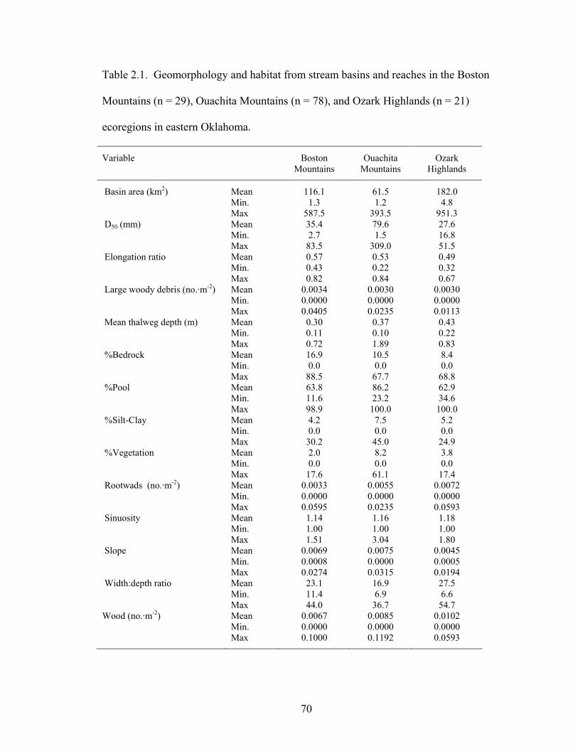
Table 2.1. Geomorphology and habitat from stream basins and reaches in the Boston

Mountains (n = 29), Ouachita Mountains (n = 78), and Ozark Highlands (n = 21)

ecoregions in eastern Oklahoma.

Variable Boston Mountains

Ouachita Mountains

Ozark Highlands

Basin area (km2) Mean 116.1 61.5 182.0 Min. 1.3 1.2 4.8 Max 587.5 393.5 951.3 D50 (mm) Mean 35.4 79.6 27.6 Min. 2.7 1.5 16.8 Max 83.5 309.0 51.5 Elongation ratio Mean 0.57 0.53 0.49 Min. 0.43 0.22 0.32 Max 0.82 0.84 0.67 Large woody debris (no.·m-2) Mean 0.0034 0.0030 0.0030 Min. 0.0000 0.0000 0.0000 Max 0.0405 0.0235 0.0113 Mean thalweg depth (m) Mean 0.30 0.37 0.43 Min. 0.11 0.10 0.22 Max 0.72 1.89 0.83 %Bedrock Mean 16.9 10.5 8.4 Min. 0.0 0.0 0.0 Max 88.5 67.7 68.8 %Pool Mean 63.8 86.2 62.9 Min. 11.6 23.2 34.6 Max 98.9 100.0 100.0 %Silt-Clay Mean 4.2 7.5 5.2 Min. 0.0 0.0 0.0 Max 30.2 45.0 24.9 %Vegetation Mean 2.0 8.2 3.8 Min. 0.0 0.0 0.0 Max 17.6 61.1 17.4 Rootwads (no.·m-2) Mean 0.0033 0.0055 0.0072 Min. 0.0000 0.0000 0.0000 Max 0.0595 0.0235 0.0593 Sinuosity Mean 1.14 1.16 1.18 Min. 1.00 1.00 1.00 Max 1.51 3.04 1.80 Slope Mean 0.0069 0.0075 0.0045 Min. 0.0008 0.0000 0.0005 Max 0.0274 0.0315 0.0194 Width:depth ratio Mean 23.1 16.9 27.5 Min. 11.4 6.9 6.6 Max 44.0 36.7 54.7 Wood (no.·m-2) Mean 0.0067 0.0085 0.0102 Min. 0.0000 0.0000 0.0000 Max 0.1000 0.1192 0.0593

70

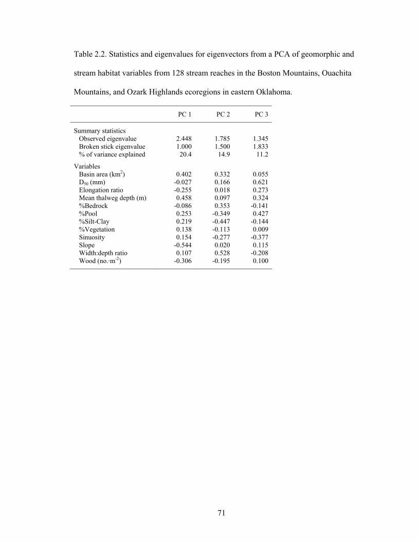
Table 2.2. Statistics and eigenvalues for eigenvectors from a PCA of geomorphic and

stream habitat variables from 128 stream reaches in the Boston Mountains, Ouachita

Mountains, and Ozark Highlands ecoregions in eastern Oklahoma.

PC 1 PC 2 PC 3

Summary statistics Observed eigenvalue 2.448 1.785 1.345 Broken stick eigenvalue 1.000 1.500 1.833 % of variance explained 20.4 14.9 11.2

Variables

Basin area (km2) 0.402 0.332 0.055 D50 (mm) -0.027 0.166 0.621 Elongation ratio -0.255 0.018 0.273 Mean thalweg depth (m) 0.458 0.097 0.324 %Bedrock -0.086 0.353 -0.141 %Pool 0.253 -0.349 0.427 %Silt-Clay 0.219 -0.447 -0.144 %Vegetation 0.138 -0.113 0.009 Sinuosity 0.154 -0.277 -0.377 Slope -0.544 0.020 0.115 Width:depth ratio 0.107 0.528 -0.208 Wood (no.·m-2) -0.306 -0.195 0.100

71

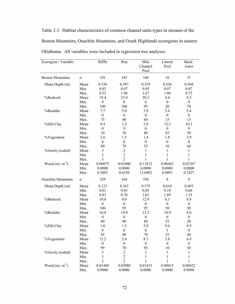
Table 2.3. Habitat characteristics of common channel units types in streams of the

Boston Mountains, Ouachita Mountains, and Ozark Highlands ecoregions in eastern

Oklahoma. All variables were included in regression tree analyses.

Ecoregion / Variable Riffle Run Mid-Channel

Pool

Lateral Pool

Back-water

Boston Mountains n 191 183 160 16 31

Mean Depth (m) Mean 0.156 0.307 0.329 0.526 0.304 Min. 0.03 0.07 0.05 0.07 0.07 Max. 0.55 1.08 1.67 1.04 0.72 %Bedrock Mean 19.4 23.9 20.3 4.4 4.2 Min. 0 0 0 0 0 Max. 100 100 95 20 70 %Boulder Mean 7.7 5.0 5.9 5.4 2.4 Min. 0 0 0 0 0 Max. 75 80 60 15 15 %Silt-Clay Mean 0.4 1.3 2.9 12.3 10.1 Min. 0 0 0 0 0 Max. 10 20 80 85 50 %Vegetation Mean 2.6 1.5 1.4 1.8 3.9 Min. 0 0 0 0 0 Max. 80 70 35 10 60 Velocity (coded) Mean 3 2 1 1 1 Min. 3 2 1 1 1 Max. 3 2 1 1 1 Wood (no.·m-2) Mean 0.00875 0.01000 0.11812 0.08463 0.02307 Min. 0.0000 0.0000 0.0000 0.0000 0.0000 Max. 0.5882 0.6250 12.0482 0.9091 0.1427

Ouachita Mountains n 259 164 356 8 9

Mean Depth (m) Mean 0.123 0.265 0.375 0.610 0.403 Min. 0.01 0.03 0.03 0.18 0.06 Max. 0.83 0.76 1.63 1.89 1.15 %Bedrock Mean 10.0 9.0 12.9 6.3 8.8 Min. 0 0 0 0 0 Max. 100 95 95 50 50 %Boulder Mean 16.4 18.0 13.2 10.9 4.0 Min. 0 0 0 0 0 Max. 80 90 80 55 20 %Silt-Clay Mean 1.0 1.5 5.0 9.6 8.9 Min. 0 0 0 1 0 Max. 45 90 70 25 40 %Vegetation Mean 13.2 5.4 8.7 3.8 6.9 Min. 0 0 0 0 0 Max. 99 70 95 10 30 Velocity (coded) Mean 3 2 1 1 1 Min. 3 2 1 1 1 Max. 3 2 1 1 1 Wood (no.·m-2) Mean 0.01460 0.05080 0.01415 0.00415 0.00422 Min. 0.0000 0.0000 0.0000 0.0000 0.0000

72

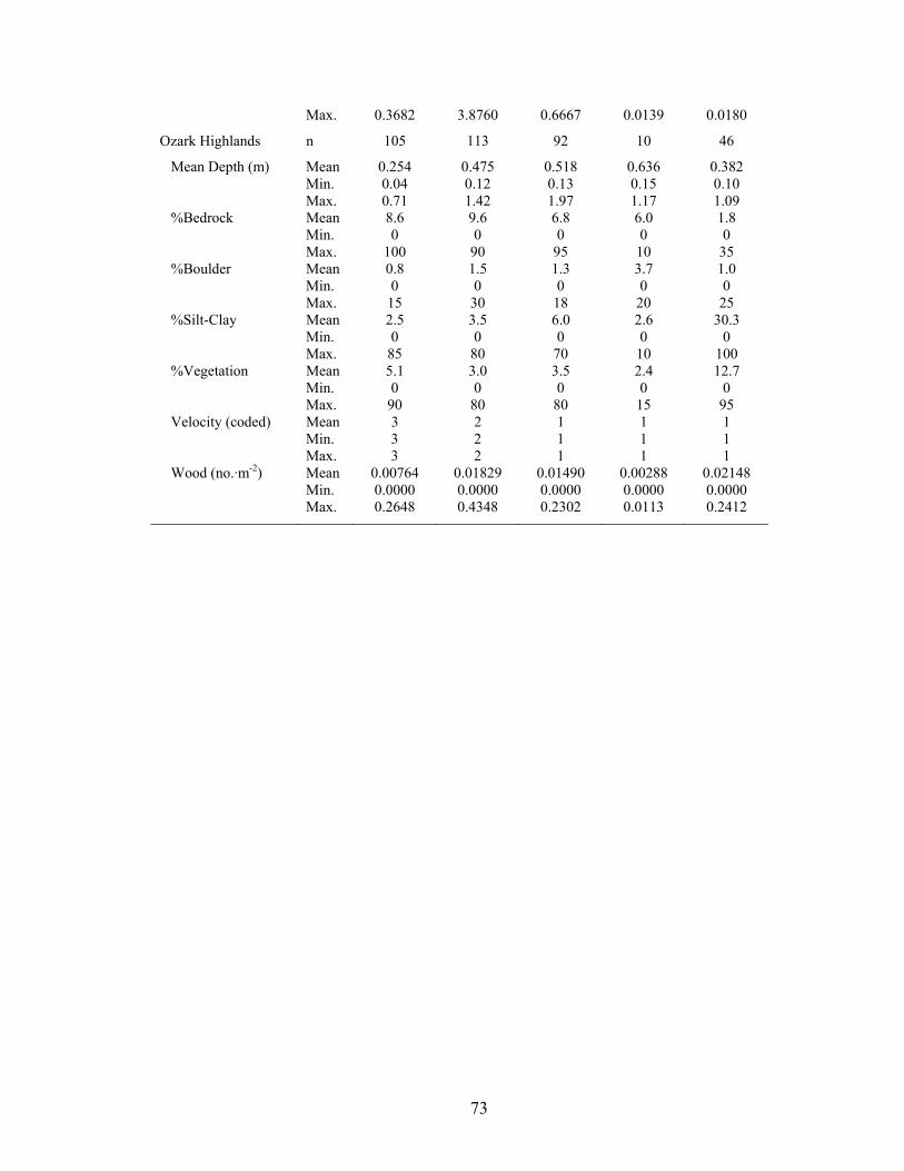
Max. 0.3682 3.8760 0.6667 0.0139 0.0180

Ozark Highlands n 105 113 92 10 46

Mean Depth (m) Mean 0.254 0.475 0.518 0.636 0.382 Min. 0.04 0.12 0.13 0.15 0.10 Max. 0.71 1.42 1.97 1.17 1.09 %Bedrock Mean 8.6 9.6 6.8 6.0 1.8 Min. 0 0 0 0 0 Max. 100 90 95 10 35 %Boulder Mean 0.8 1.5 1.3 3.7 1.0 Min. 0 0 0 0 0 Max. 15 30 18 20 25 %Silt-Clay Mean 2.5 3.5 6.0 2.6 30.3 Min. 0 0 0 0 0 Max. 85 80 70 10 100 %Vegetation Mean 5.1 3.0 3.5 2.4 12.7 Min. 0 0 0 0 0 Max. 90 80 80 15 95 Velocity (coded) Mean 3 2 1 1 1 Min. 3 2 1 1 1 Max. 3 2 1 1 1 Wood (no.·m-2) Mean 0.00764 0.01829 0.01490 0.00288 0.02148 Min. 0.0000 0.0000 0.0000 0.0000 0.0000 Max. 0.2648 0.4348 0.2302 0.0113 0.2412

73

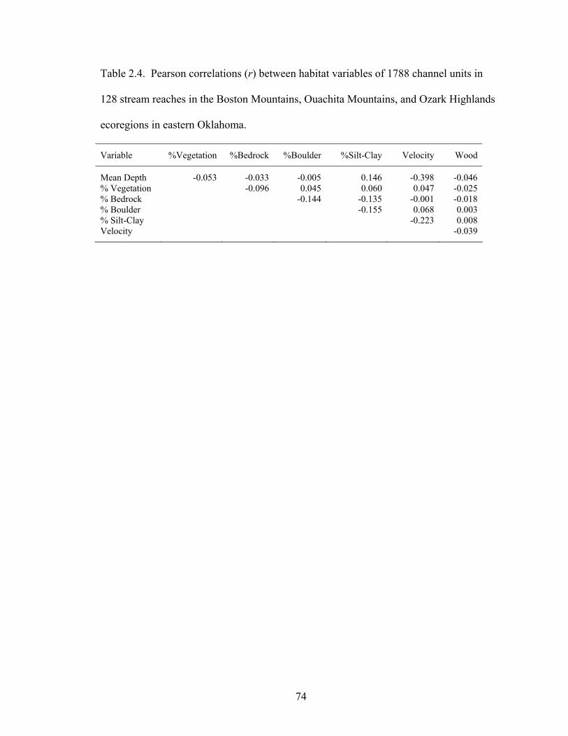
Table 2.4. Pearson correlations (r) between habitat variables of 1788 channel units in

128 stream reaches in the Boston Mountains, Ouachita Mountains, and Ozark Highlands

ecoregions in eastern Oklahoma.

Variable %Vegetation %Bedrock %Boulder %Silt-Clay Velocity Wood

Mean Depth -0.053 -0.033 -0.005 0.146 -0.398 -0.046 % Vegetation -0.096 0.045 0.060 0.047 -0.025 % Bedrock -0.144 -0.135 -0.001 -0.018 % Boulder -0.155 0.068 0.003 % Silt-Clay -0.223 0.008 Velocity -0.039

74

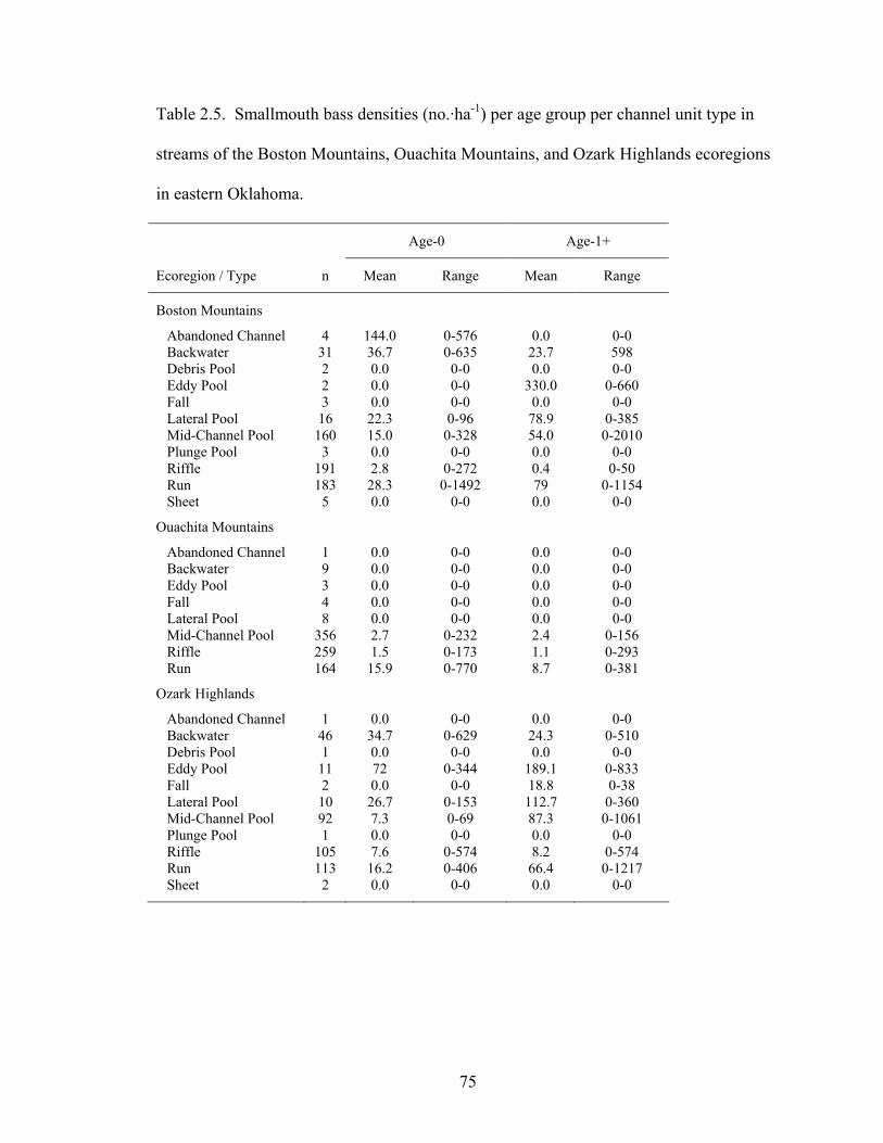
Table 2.5. Smallmouth bass densities (no.·ha-1) per age group per channel unit type in

streams of the Boston Mountains, Ouachita Mountains, and Ozark Highlands ecoregions

in eastern Oklahoma.

Age-0 Age-1+

Ecoregion / Type n Mean Range Mean Range

Boston Mountains

Abandoned Channel 4 144.0 0-576 0.0 0-0 Backwater 31 36.7 0-635 23.7 598 Debris Pool 2 0.0 0-0 0.0 0-0 Eddy Pool 2 0.0 0-0 330.0 0-660 Fall 3 0.0 0-0 0.0 0-0 Lateral Pool 16 22.3 0-96 78.9 0-385 Mid-Channel Pool 160 15.0 0-328 54.0 0-2010 Plunge Pool 3 0.0 0-0 0.0 0-0 Riffle 191 2.8 0-272 0.4 0-50 Run 183 28.3 0-1492 79 0-1154 Sheet 5 0.0 0-0 0.0 0-0

Ouachita Mountains

Abandoned Channel 1 0.0 0-0 0.0 0-0 Backwater 9 0.0 0-0 0.0 0-0 Eddy Pool 3 0.0 0-0 0.0 0-0 Fall 4 0.0 0-0 0.0 0-0 Lateral Pool 8 0.0 0-0 0.0 0-0 Mid-Channel Pool 356 2.7 0-232 2.4 0-156 Riffle 259 1.5 0-173 1.1 0-293 Run 164 15.9 0-770 8.7 0-381

Ozark Highlands

Abandoned Channel 1 0.0 0-0 0.0 0-0 Backwater 46 34.7 0-629 24.3 0-510 Debris Pool 1 0.0 0-0 0.0 0-0 Eddy Pool 11 72 0-344 189.1 0-833 Fall 2 0.0 0-0 18.8 0-38 Lateral Pool 10 26.7 0-153 112.7 0-360 Mid-Channel Pool 92 7.3 0-69 87.3 0-1061 Plunge Pool 1 0.0 0-0 0.0 0-0 Riffle 105 7.6 0-574 8.2 0-574 Run 113 16.2 0-406 66.4 0-1217 Sheet 2 0.0 0-0 0.0 0-0

75

Figure 2.1. Sites selected (175) and sampled (128) for an inventory of fluvial

geomorphology, stream habitat, and smallmouth bass in eastern Oklahoma streams.

Figure 2.2. PCA biplots of geomorphology and habitat of 128 stream reaches in three

eastern Oklahoma ecoregions. Axis 1 represented stream size, where slope (-0.544),

mean thalweg depth (0.458), and basin area (0.402) had the highest axis loadings. Axis 2

represented channel stability; width:depth ratio (0.528), percent silt-clay (-0.447), and

percent bedrock (0.353) had high axis loadings. D50 (0.621), percent pool (0.427), and

sinuosity (-0.377) had high axis loadings for axis 3.

Figure 2.3. Regression tree analysis of effects of ecoregion, basin and reach

geomorphology and habitat, and channel unit habitat on age-0 smallmouth bass densities

(no.·ha-1) in 1788 channel units from 128 stream reaches in three eastern Oklahoma

ecoregions. Mean densities per node are given, with sample sizes in parentheses.

Observations with variable values less than or equal to node value split to the left, and

values greater than split right. Terminal nodes are oval. 10-fold cross-validated relative

error was 0.825.

Figure 2.4. Regression tree analysis of effects of ecoregion, basin and reach

geomorphology and habitat, and channel unit habitat on age-1+ smallmouth bass

densities (no.·ha-1) in 1788 channel units from 128 stream reaches in three eastern

Oklahoma ecoregions. Mean densities per node are given, with sample sizes in

parentheses. Observations with variable values less than or equal to node value split to

76

the left, and values greater than split right. Terminal nodes are oval. 10-fold cross-

validated relative error was 0.627. Broad descriptions of channel units related to primary

splits are given.

77

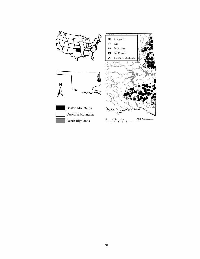
78

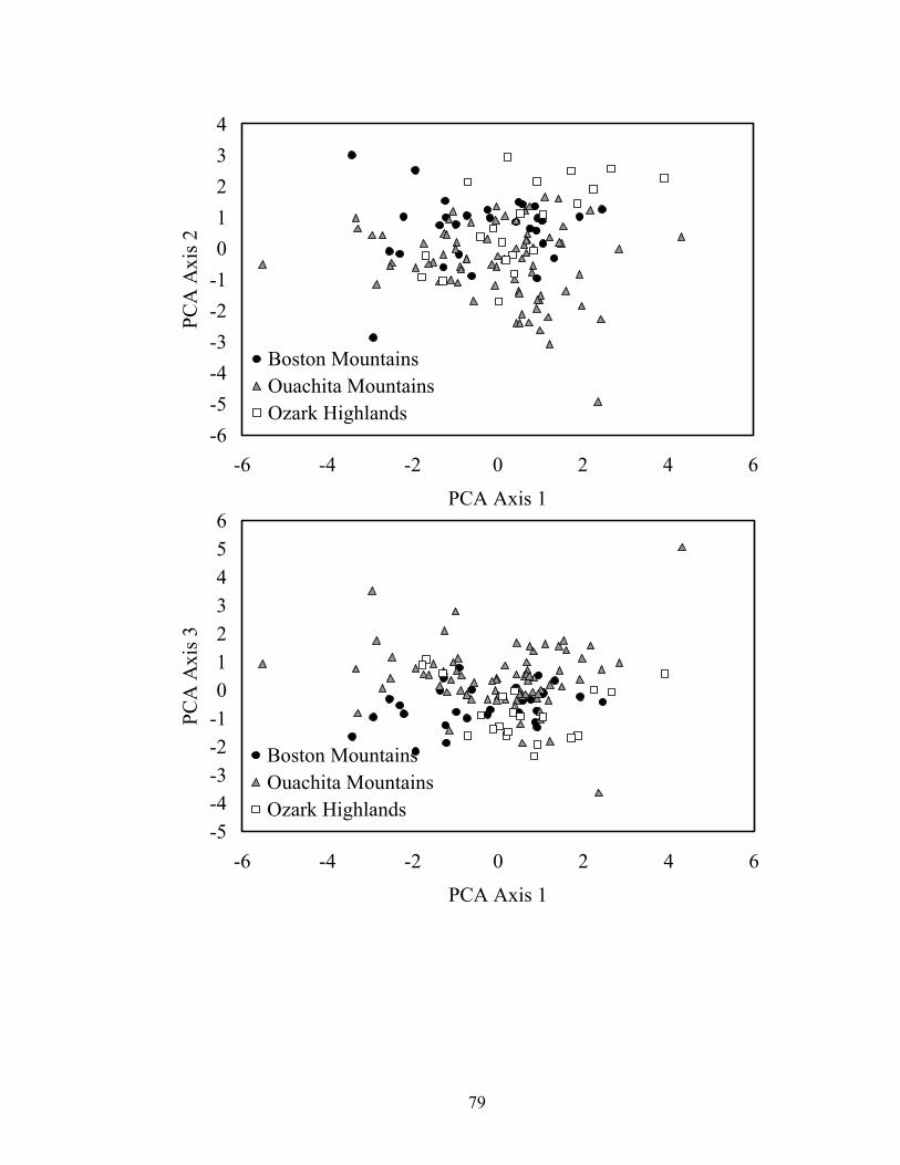
-5-4-3-2-10123456

-6 -4 -2 0 2 4 6

PCA Axis 1

PCA

Axi

s 3

Boston MountainsOuachita MountainsOzark Highlands

-6-5-4-3-2-101234

-6 -4 -2 0 2 4 6

PCA Axis 1

PCA

Axi

s 2

Boston MountainsOuachita MountainsOzark Highlands

79

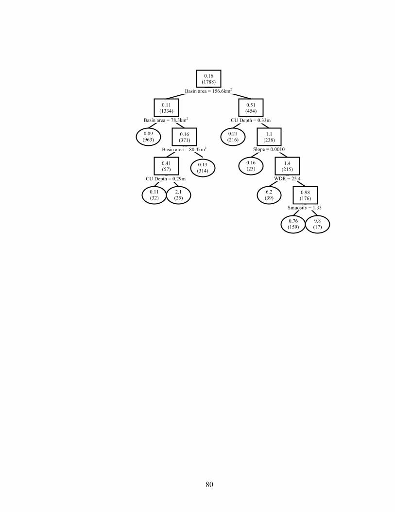
0.16 (1788)

0.51 (454)

0.09 (963)

0.21 (216)

0.16 (23)

Basin area = 156.6km2

CU Depth = 0.33m

0.11 (1334)

0.16 (371)

0.41 (57)

1.1 (238)

1.4 (215)

0.98 (176)

0.13 (314)

0.11 (32)

0.76 (159)

9.8 (17)

6.2 (39)

2.1 (25)

CU Depth = 0.29m

Basin area = 78.3km2

Basin area = 80.4km2 Slope = 0.0010

WDR = 25.4

Sinuosity = 1.35

80

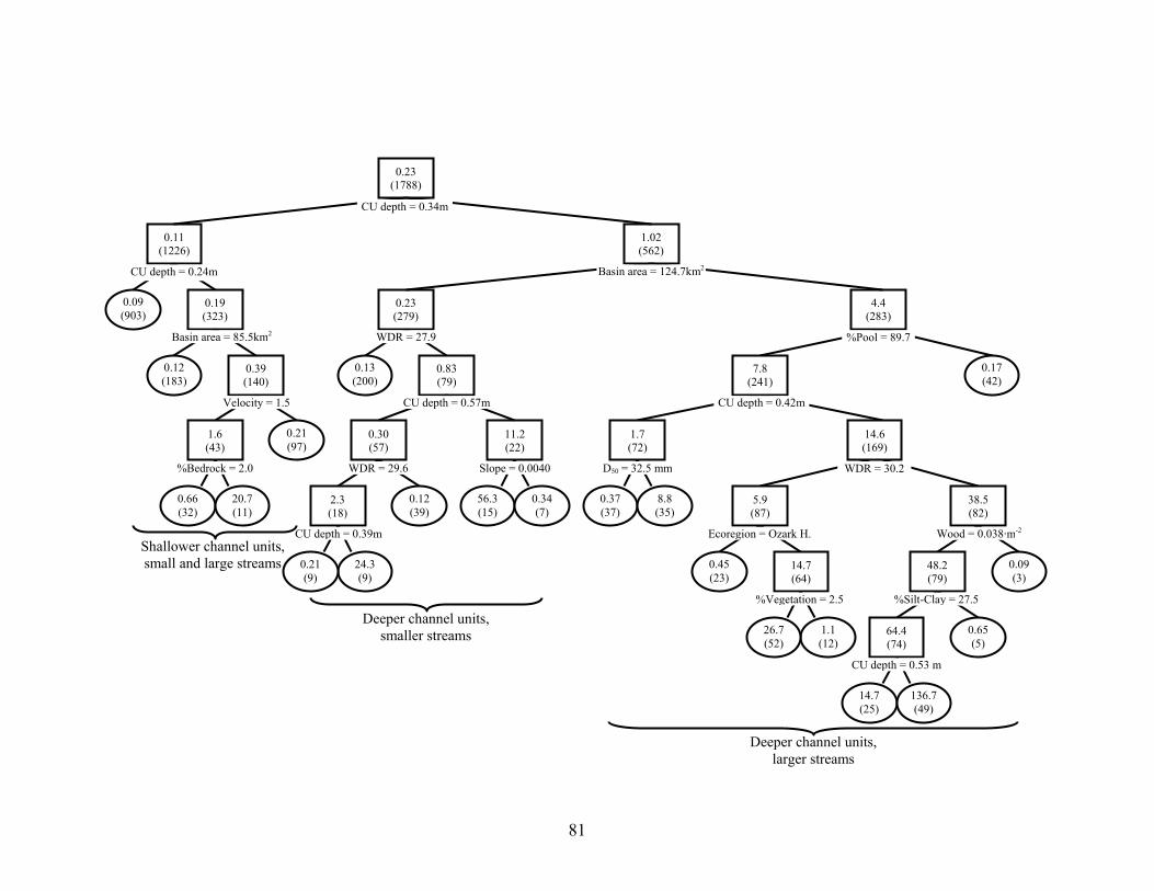
1.02 (562)

0.11 (1226)

0.23 (1788)

7.8 (241)

0.83 (79)

0.39 (140)

4.4 (283)

0.23 (279)

0.19 (323)

1.6 (43)

0.30 (57)

11.2 (22)

1.7 (72)

14.6 (169)

2.3 (18)

38.5 (82)

5.9 (87)

48.2 (79)

64.4 (74)

0.09 (903)

0.12 (183)

0.13 (200)

0.17 (42)

0.66 (32)

20.7 (11)

0.12 (39)

56.3 (15)

0.34 (7)

24.3 (9)

0.21 (9)

0.45 (23)

0.37 (37)

8.8 (35)

0.65 (5)

14.7 (25)

0.21 (97)

CU depth = 0.34m

CU depth = 0.24m

Basin area = 85.5km2

Velocity = 1.5

%Bedrock = 2.0

Basin area = 124.7km2

WDR = 27.9

CU depth = 0.57m

WDR = 29.6

CU depth = 0.39m

Slope = 0.0040

%Pool = 89.7

CU depth = 0.42m

D50 = 32.5 mm WDR = 30.2

Wood = 0.038·m-2

%Silt-Clay = 27.5

136.7 (49)

0.09 (3)

14.7 (64)

%Vegetation = 2.5

CU depth = 0.53 m

Shallower channel units, small and large streams

Deeper channel units, smaller streams

Ecoregion = Ozark H.

1.1 (12)

26.7 (52)

Deeper channel units, larger streams

81

Appendix 2.A. Snorkeling and electrofishing methods for estimating smallmouth bass

abundance.

Snorkeling model

Methods

We developed a linear model to adjust snorkeling counts of smallmouth bass to obtain

abundance estimates. The model was developed by using data whereby 21 channel units

were snorkeled, and smallmouth bass < and ≥100mm were counted. The same channel

units were then electrofished, and an electrofishing abundance estimate was made by

adjusting the number in individuals collected by the 3-pass predicted capture probability

(see below). Channel-unit habitat was also measured and estimated (see Methods).

Multiple linear regression and forward selection of fish size and habitat variables

(variable entry, P ≤ 0.15) was used to predict: snorkeling counts:electrofishing abundance

estimates. We could not use logistic regression because snorkeling counts were

sometimes greater than abundance estimates. In addition to fish size, the habitat

variables evaluated for their effect on snorkeling counts were: water clarity (m); mean

thalweg depth (m); wood density (no.·m-2); and channel-unit width (m). Statistical

Analysis Systems software, version 9.1 (SAS Institute Inc., Cary, North Carolina) was

used to fit a model of 42 observations (21 channel units · 2 size classes). Studentized

deleted residuals were plotted against explanatory variables to assess heteroscedasticity.

Results

82

Forward selection included no fish size or habitat variable in the model. Thus, we fit a

direct proportion model (no intercept) to predict abundance estimates from snorkel

counts. The final model was:

(1) = 1.3529(snorkeling count) N

Model fit was: r2 = 0.617. Residual plots revealed homogeneity of error variance.

Results demonstrated that snorkelers adjusted their searches, as intended, to account for

habitat complexity within channel units, and were equally effective at observing small

and large fishes.

Electrofishing model

Methods

Mark-recapture data were used to develop a 1- and 3-pass capture probability model to

estimate smallmouth bass abundance in channel units. In 24 channel units in two eastern

Oklahoma streams, smallmouth bass were collected, marked, and returned. Habitat

variables measured were: mean thalweg depth (m), %bedrock, %silt-clay, wood density

(no.·m-2). After a recovery period, three electrofishing passes were made to recapture

individuals. Capture probability for 1 and 3 electrofishing passes was estimated using

multiple logistic regression and Statistical Analysis Systems software, version 9.1 (SAS

Institute Inc., Cary, North Carolina) with fish size (< and ≥100 mm), electrofishing power

(µS·cm-3), and all habitat variables as potential explanatory variables:

(2) 110 ....)]ˆˆexp(1[ˆ −−−+= ixp ββ

All combinations of explanatory variables, including fish size×depth, depth×%bedrock

and depth×%silt-clay interactions, were evaluated using model selection and averaging

83

methods. Abundance estimates were obtained by correcting number of individuals

collected by model averaged, predicted capture probability, . 1ˆˆ −⋅= pCN

Results

All habitat variables, except mean thalweg depth×%silt-clay interaction, were included in

at least one candidate model (Table 2.A.1). Fish size and mean thalweg depth, and their

interaction, had the largest effect on capture probabilities (Table 2.A.2). Precision of

abundance estimates from the 1-pass model, when compared to known abundances using

linear regression, were lower (r2 = 0.769) than precision for the 3-pass model (r2 =

0.881), but both models produced unbiased abundance estimates (bi = 1, P ≥ 0.462).

84

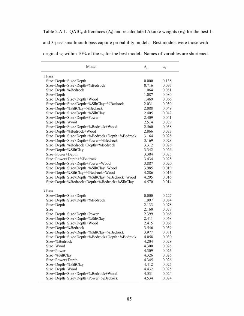
Table 2.A.1. QAICc differences (∆i) and recalculated Akaike weights (wi) for the best 1-

and 3-pass smallmouth bass capture probability models. Best models were those with

original wi within 10% of the wi for the best model. Names of variables are shortened.

Model ∆i wi

1 Pass Size+Depth+Size×Depth 0.000 0.138 Size+Depth+Size×Depth+%Bedrock 0.716 0.097 Size+Depth+%Bedrock 1.064 0.081 Size+Depth 1.087 0.080 Size+Depth+Size×Depth+Wood 1.469 0.066 Size+Depth+Size×Depth+%SiltClay+%Bedrock 2.031 0.050 Size+Depth+%SiltClay+%Bedrock 2.088 0.049 Size+Depth+Size×Depth+%SiltClay 2.405 0.042 Size+Depth+Size×Depth+Power 2.409 0.041 Size+Depth+Wood 2.514 0.039 Size+Depth+Size×Depth+%Bedrock+Wood 2.560 0.038 Size+Depth+%Bedrock+Wood 2.866 0.033 Size+Depth+Size×Depth+%Bedrock+Depth×%Bedrock 3.164 0.028 Size+Depth+Size×Depth+Power+%Bedrock 3.169 0.028 Size+Depth+%Bedrock+Depth×%Bedrock 3.312 0.026 Size+Depth+%SiltClay 3.342 0.026 Size+Power+Depth 3.384 0.025 Size+Power+Depth+%Bedrock 3.434 0.025 Size+Depth+Size×Depth+Power+Wood 3.887 0.020 Size+Depth+Size×Depth+%SiltClay+Wood 3.985 0.019 Size+Depth+%SiltClay+%Bedrock+Wood 4.286 0.016 Size+Depth+Size×Depth+%SiltClay+%Bedrock+Wood 4.295 0.016 Size+Depth+%Bedrock+Depth×%Bedrock+%SiltClay 4.570 0.014 3 Pass Size+Depth+Size×Depth 0.000 0.227 Size+Depth+Size×Depth+%Bedrock 1.997 0.084 Size+Depth 2.133 0.078 Size 2.160 0.077 Size+Depth+Size×Depth+Power 2.399 0.068 Size+Depth+Size×Depth+%SiltClay 2.411 0.068 Size+Depth+Size×Depth+Wood 2.415 0.068 Size+Depth+%Bedrock 3.546 0.039 Size+Depth+Size×Depth+%SiltClay+%Bedrock 3.977 0.031 Size+Depth+Size×Depth+%Bedrock+Depth×%Bedrock 4.058 0.030 Size+%Bedrock 4.204 0.028 Size+Wood 4.300 0.026 Size+Power 4.309 0.026 Size+%SiltClay 4.326 0.026 Size+Power+Depth 4.345 0.026 Size+Depth+%SiltClay 4.412 0.025 Size+Depth+Wood 4.432 0.025 Size+Depth+Size×Depth+%Bedrock+Wood 4.531 0.024 Size+Depth+Size×Depth+Power+%Bedrock 4.534 0.024

85

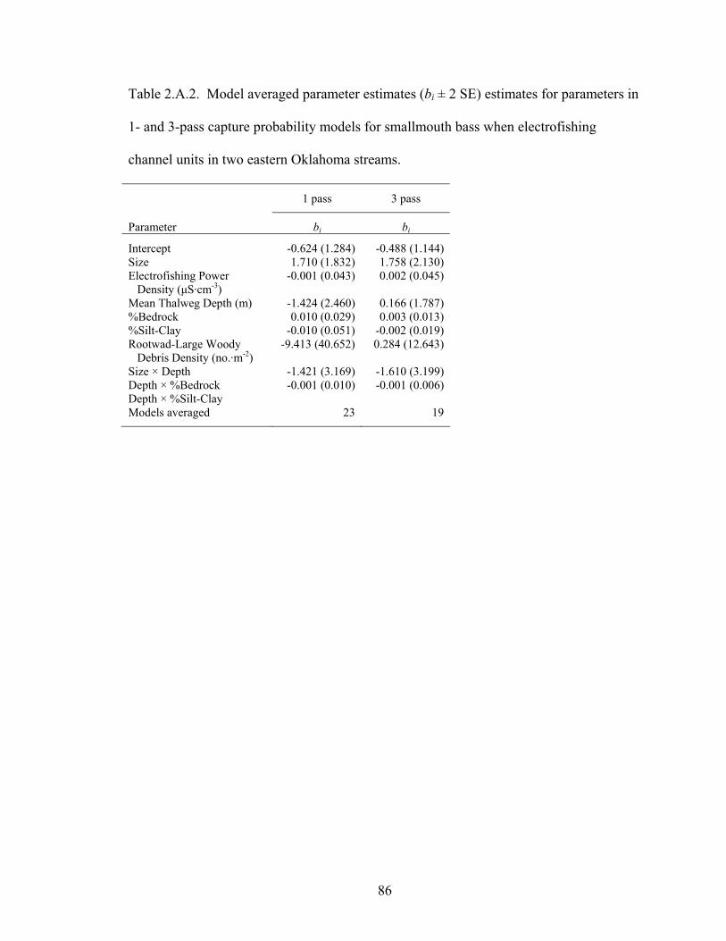
Table 2.A.2. Model averaged parameter estimates (bi ± 2 SE) estimates for parameters in

1- and 3-pass capture probability models for smallmouth bass when electrofishing

channel units in two eastern Oklahoma streams.

1 pass 3 pass

Parameter bi bi

Intercept -0.624 (1.284) -0.488 (1.144) Size 1.710 (1.832) 1.758 (2.130) Electrofishing Power Density (µS·cm-3)

-0.001 (0.043) 0.002 (0.045)

Mean Thalweg Depth (m) -1.424 (2.460) 0.166 (1.787) %Bedrock 0.010 (0.029) 0.003 (0.013) %Silt-Clay -0.010 (0.051) -0.002 (0.019) Rootwad-Large Woody Debris Density (no.·m-2)

-9.413 (40.652) 0.284 (12.643)

Size × Depth -1.421 (3.169) -1.610 (3.199) Depth × %Bedrock -0.001 (0.010) -0.001 (0.006) Depth × %Silt-Clay Models averaged 23 19

86

CHAPTER 3

SMALLMOUTH BASS POPULATIONS AND STREAM HABITAT IN EASTERN

OKLAHOMA: SPATIOTEMPORAL PATTERNS AND HABITAT

COMPLEMENTATION AND SUPPLEMENTATION

87

Abstract

Spatial and temporal dynamics of stream habitat and fish populations are important

considerations for the conservation and management of stream fishes. We determined

differences in stream habitat and smallmouth bass Micropterus dolomieu demographics

among stream orders 3 – 5 in two regional streams in eastern Oklahoma from 2003 to

2005. Water temperature, streamflow, and habitat differed between streams and

longitudinally within streams. Recruitment variability of smallmouth bass was highest in

upstream reaches of both streams, and higher in Glover River than Baron Fork Creek in

reaches with the highest smallmouth bass densities. Survival was higher in Baron Fork

Creek than Glover River and was typically lowest from summer to fall in both streams.

Relative growth in length of smallmouth bass was not different between streams or ages,

but was highest from summer to fall. Relative weights were higher in Baron Fork Creek

than Glover River in upstream reaches, and decreased linearly as stream order increased

in Baron Fork Creek but not in Glover River. Relative weights were lowest in spring and

highest in summer in both streams. Movement among channel units was highest from

fall to winter, and there was evidence that older individuals moved more. Habitat

complementation was evident whereby smallmouth bass used different channel units for

spawning versus winter thermal refugia. However, food and cover were apparently

substitutable or ubiquitous and supplemented in different habitats because they did not

strongly affect distributions of individuals in summer and fall. Integrating spatiotemporal

patterns in stream habitat and population demographics with knowledge of habitat

complementation and supplementation is important for conservation and management of

habitat and fishes in stream resources that provide important angling opportunities.

88

Introduction

A critical element in the conservation and management of a fish population is to

understand factors affecting population demographics. Stream habitat and its constituent

components reflect a myriad of physical and biological processes acting on hierarchically

nested spatial and temporal scales (Frissell et al. 1986). Habitat is often regarded as a

major factor affecting stream fish populations and structuring fish assemblages (Gorman

and Karr 1978). Habitats are defined according to whether their components (abiotic and

biotic) are consumed directly by fishes and their supply is affected by fish density (Hayes

et al. 1996). The consumable and dynamic properties of habitat components determine

the relationship between habitat and fish population dynamics.

Although specific habitats can affect fish population dynamics, it is important to

understand the spatial and temporal distribution of all habitats needed by fishes to

complete life processes. Many fish species use different habitats to reproduce, feed and

grow, and seek refuge from harsh environmental conditions (Figure 3.1; Schlosser 1991;

Schlosser 1995). An area of a stream system that contains all needed habitats has been

defined as a functional habitat unit (Kocik and Ferreri 1998). Schlosser (1995) suggested

that habitat complementation (different habitats with non-substitutable resources), habitat

supplementation (different habitats with substitutable resources), source-sink interactions

(spatial variation in juvenile production), and neighborhood effects (spatial structure and

connectivity of habitats) influence fish population dynamics. Movement of fishes into

and out of habitats (turnover) has been used as a measure of habitat quality (Bélanger and

Rodríguez 2002) and has energetic and predation costs. Thus, high levels of habitat

89

supplementation (versus complementation) and smaller functional habitat units would

result in population dynamics leading to large local population sizes, and more functional

habitat units in a system would result in higher abundances of a fish species within a

stream system. Kocik and Ferreri (1998) demonstrated how incorporating the spatial

structure (interspersion and juxtaposition) of functional habitat units (including spawning

and rearing habitat) increased the predicted production of juveniles and decreased

extirpation probabilities of Atlantic salmon Salmo salar in the Narraguagas River, Maine.

Fausch et al. (2002) suggested that information critical to conservation of stream fish

populations is needed at intermediate spatial scales (10 – 10,000 m), because such scales

likely encompass the size of functional habitat units of most fish species. They also

recommended that information be collected continuously throughout the river network in

order to document specific critical habitats or disturbances that might be missed under

probabilistic sampling designs.

The smallmouth bass Micropterus dolomieu is both a popular sport fish and an

indicator of habitat conditions. The species has been introduced into waters outside of its

native range for angling opportunities (the Mississippi and Great Lakes drainages;

MacCrimmon and Robbins 1975) and is now found throughout most of North America

and in many parts of the World in both lakes and streams (Jackson 2002). The

smallmouth bass generally inhabits clear, coolwater streams with notable current and

gravel substrates (Coble 1975). Microhabitat studies show that suitability of

microhabitats (e.g., water velocity and depth, cover) change with life stage, and may

differ among streams (Groshens and Orth 1993; Orth and Newcomb 2002). At larger

spatial scales, variability in abundance of smallmouth bass exists within and among

90

streams. Smallmouth bass abundance is typically unimodal along the longitudinal

gradient of a stream: abundances are lower in headwater streams (Coble 1975; Lyons

1991) and in larger downstream reaches where smallmouth bass are replaced by

largemouth bass M. salmoides (Rabeni and Jacobson 1993a; Sowa and Rabeni 1995),

often in response to different geomorphic processes and land use practices that have

population level effects (Rabeni and Sowa 1996). Regional differences in smallmouth

bass population characteristics likely reflect landscape features (Stark and Zale 1991).

Studies conducted at different spatial scales (sensu Frissell et al. 1986) have all elucidated

important information about stream habitat associations with smallmouth bass

populations (Rabeni and Sowa 1996).

Smallmouth bass, in addition to the other black basses (spotted M. punctulatus

and largemouth bass), are generally preferred by stream anglers in eastern Oklahoma

(Fisher et al. 2002). Smallmouth bass demographics apparently differ between regions in

eastern Oklahoma (Stark and Zale 1991; Balkenbush and Fisher 2001), but longitudinal

and seasonal changes in abundance have not been related to population dynamics (Pezold

et al. 1997; Walsh 2003; Walsh and Winkelman 2004a). Additionally, these spatial and

temporal changes have not been evaluated in a stream habitat context. Our objectives

were: 1) to determine how stream habitat and smallmouth bass population demographics

vary spatially and temporally between and within two regional streams in eastern

Oklahoma, and 2) evaluate habitat complementation and supplementation patterns within

these streams. Understanding spatial and temporal variation in stream habitat and how

population characteristics are related to that habitat will advance understanding of stream

processes influencing smallmouth bass populations. This understanding is needed to

91

guide conservation and management strategies aimed at protecting and enhancing stream

habitats that influence demographic rates of smallmouth bass that influence population

size.

Methods

Study streams

We sampled smallmouth bass populations and surveyed stream habitat in three

reaches each on Baron Fork Creek and Glover River (Figure 3.2). Baron Fork Creek

originates in northwest Arkansas and flows west-southwest through the Boston

Mountains and Ozark Highlands ecoregions to its confluence with the Illinois River at

Lake Tenkiller, Oklahoma. The Boston Mountains ecoregion is a dissected mountainous

plateau composed of flat-lying shale and sandstone lithology and oak-hickory forest.

Annual rainfall is 112 to 130 cm and land use is mostly logging and recreation (Woods et

al. 2005). The Ozark Highlands are dominated by flat-lying cherty limestone, but shale,

limestone, and dolomite are present in valley bottoms. Annual precipitation is 104 to 124

cm, and land use is primarily logging, recreation, and cattle and poultry farming,

including pastureland and hayfields (Rabeni and Jacobson 1993a; Woods et al. 2005).

Baron Fork Creek has hard water (60-99 mg/l CaCO3; Balkenbush and Fisher 2001).

Mean annual streamflow upstream for Baron Fork Creek at Dutch Mills, Arkansas

(United States Geological Survey [USGS] gauge 07196900; period of record, 1958 to

2005) was 1.3 m3/s (CV = 540), and 9.3 m3/s (CV = 560) downstream at Eldon,

Oklahoma (USGS gauge 07197000; 1948 to 2004). The Glover River flows south,

mainly through the Ouachita Mountains, to its confluence with the Little River,

92

Oklahoma. The Ouachita Mountains consist of folded, Paleozoic sandstone, shale, and

chert lithology. Oak-hickory-shortleaf pine forests in this region receive from 109 to 145

cm of annual rainfall. Common land uses are logging, pastureland, hayfields, farming,

and recreation (Rutherford et al. 1992; Woods et al. 2005). Glover River has turbid, soft

water (12-38 mg/l CaCO3; Balkenbush and Fisher 2001). Mean annual streamflow for

the lower Glover River near Glover, Oklahoma was 14.1 m3/s (CV = 540) (USGS gauge

07337900; 1961 to 2004). Small floods, defined as a streamflow pulse that has a

recurrence interval of 2 years, have durations (median days ± [75th - 25th]/50th

percentiles; Indicators of Hydrologic Alteration software, Version 7, The Nature

Conservancy) that indicate the lower Glover River is flashier (26 d ± 0.93) than both

upper (30 d ± 1.28) and lower (32 d ± 0.84) Baron Fork Creek.

Sampling

Water temperature and streamflow were measured or estimated for each reach.

Water temperatures were recorded every 1 to 2 hr at each reach using StowAway®

Tidbit® temperature loggers (Onset Computer Corporation, Bourne, Massachusetts) in

Baron Fork Creek, and Solinst Levelloggers® (Solinst Canada Ltd., Georgetown, Ontario)

in Glover River. Streamflow for each reach was prorated using USGS gauging station

data. Estimates were made by relating measured discharge (Gallagher and Stevenson

1999) at each reach on multiple dates to USGS gauge data. A proportional model was

then used to adjust gauge data to obtain reach estimates. Gauge 07196900 at Dutch

Mills, Arkansas was used to estimate streamflow at the 3rd and 4th order reaches on Baron

Fork Creek, and gauge 07197000 at Eldon was used to prorate streamflow at the 5th order

93

reach. Gauge 07337900 near Glover, Oklahoma was used to estimate streamflow at all

three Glover River reaches. Streamflow was only estimated from 15 July 2003 to 15 July

2004 because only provisional data were available after 30 September 2004.

Study sites on Baron Fork Creek and Glover River were located on 3rd, 4th, and 5th

order stream reaches. We sampled 3rd and 4th order reaches once each season, and the 5th

order sites during summer and fall; streamflows prohibited sampling at the 5th order sites

during winter and spring. We conducted spring sampling in late March, summer

sampling from late July to early August, fall sampling in mid-October, and winter

sampling from mid-December to mid-January from July 2003 to August 2005.

During each sampling period, channel units were identified and classified within a

defined reach 20+ times the mean channel width. All channel units were classified using

the scheme of Hawkins et al. (1993), and they were mapped with a global positioning

system (GPS) and measured in a GIS (Dauwalter et al. 2006). Mapping with a GPS and

GIS allowed quantification of channel unit areas and relative positions. Thalweg depths

were measured multiple times per channel unit; more measurements were made in longer

channel units. A modified Wentworth scale was used to visually estimate substrate

distributions of silt (<0.059 mm), sand (0.06-1.00 mm), gravel (2-15 mm), pebble (16-63

mm), cobble (64-256 mm), boulders (>256 mm), and bedrock (Bain 1999) within each

channel unit. We estimated, and enumerated when logistically feasible, boulders,

rootwads, and large woody debris (10+ cm diameter, 4+ m in length) in each channel

unit.

We collected fish within each channel unit (except riffles) by using multi-pass

backpack, barge, or boat electrofishing. Each channel unit was block netted (≤ 6.35 mm

94

mesh), except in Glover River reaches in winter and spring when elevated streamflows

and large surficial substrates prohibited effective block netting. Two electrofishing

passes were conducted, and if one or more smallmouth bass were collected in the first

two passes a third pass was made. Smallmouth bass collected during electrofishing were

measured (TL) and weighed. Scales were taken posterior to the pectoral fin from

individuals >90 mm TL for age analysis (individuals could not be sacrificed for otoliths),

and individuals were tagged with a Floy t-bar anchor tag adjacent to the dorsal fin. A

subsample of individuals was double tagged to estimate tag retention. Individuals were

then returned to the channel unit from which they were captured after a recovery period.

Crayfish were collected from a subset of channel units at 4th order sites with a 1-m2

quadrat sampler (DiStefano et al. 2003) as an index of prey abundance (Probst et al.

1984). Voucher specimens were preserved on site and identified in the laboratory

(Pflieger 1996). One to nine quadrat samples were collected per channel unit.

Smallmouth bass scales collected for age analysis were pressed onto acetate

microscope slides, and aged by two readers. A third reader was used when ages differed

between the first two readers. Individuals <90 mm were assumed to be age-0

(Balkenbush and Fisher 2001). Hatch dates were assigned between spring and summer

samples in correspondence with the late-spring spawning season.

Statistical analyses

Unless otherwise noted, analyses were done in SAS Version 9.1 software (PROC

MIXED and GENMOD; SAS Institute, Inc., Cary, North Carolina). Type I error rate was

set at α = 0.05. A Kenward-Roger degrees of freedom adjustment was used if variances

95

were unequal, sometimes resulting in fractional degrees of freedom (Kenward and Roger

1997). Linear contrasts were used to assess differences between streams, seasons, and

ages when applicable, and polynomial contrasts were used to evaluate trends with stream

order (Kuehl 2000).

Recruitment variability

We used residuals from a weighted catch-curve analysis to estimate smallmouth

bass recruitment variability for each reach (Maceina 1997). A weighted catch-curve

analysis regresses loge(number individuals collected) against age, and uses loge(number

individuals collected) as the weight. Higher coefficients of determination (r2) from

regressions for each reach indicated lower recruitment variability. Data from July and

October 2003 samples were pooled and used for analysis of Baron Fork Creek reaches,

and August and October 2004 samples were pooled and used for the Glover River.

Seasonal survival and recapture rates

We evaluated apparent survival and recapture rates of smallmouth bass by age

class and season for each reach and season. All individuals that died from sampling were

excluded from analyses. We modeled apparent survival and recapture rates by using an

open population, time-independent model (Williams et al. 2002), and used model

selection to evaluate a set of candidate models. Apparent survival is actual survival

multiplied by permanent immigration (not estimated); hereafter, we refer to apparent

survival as survival. A model including seasonal and age (1, 2, and 3+) effects in both

survival and recapture rates was used as the global model. Fit of the global model was

96

evaluated by comparing observed model deviance to a distribution of bootstrapped

deviance estimates from 500 simulations (Burnham and Anderson 2002). Other models

evaluated were subsets of the global model that included combinations of: 1) age and

season or season effects only on survival, and 2) age and season, age only, and season

only effects on recapture rates or constant recapture rates. Models were compared using

Akaike’s Information Criterion corrected for small sample bias (AICc, or QAICc when

overdispersion was evident), and model averaging was conducted using Akaike weights

(Burnham and Anderson 2002). Survival estimates were adjusted for three-month tag

retention rates (Arnason and Mills 1981). All analyses were done using Program MARK

(White and Burnham 1999).

Relative growth rates

Relative daily growth rates in length and weight (% initial body length or weight

per day) were measured using individuals recaptured in successive seasons (Busacker et

al. 1990). Fixed effects of stream, season, and age (at the end of the season) on relative

growth were determined by using a mixed model with year as a random effect. The only

interaction tested was age×season.

Condition

We determined the effects of stream, stream order, and season on condition of

smallmouth bass. Condition was determined using relative weights of individuals ≥160

mm (Kolander et al. 1993). Differences in condition were determined using a mixed

model whereby stream, stream order, and season were treated as fixed effects and year

97

was treated as a random variable. A stream×stream order interaction was included in the

model.

Within reach movements

We evaluated seasonal within reach movements of smallmouth bass by

determining how many individuals moved from one channel unit to another between

successive seasons. A descriptive multiple logistic regression model was developed to

determine the effects of season, age, reach and year on movement probability. Season

was modeled as a dummy variable, with winter as the baseline. Adequacy of model fit

was determined using a Hosmer-Lemeshow test (Hosmer and Lemeshow 2000).

Densities and size structure in channel units

We determined how abundance of age-0 and age-1+ smallmouth bass, and mean

size of age-1+ individuals, differed among channel units between streams, stream order,

and seasons, and how they were related to habitat within channel units. Relations were

determined using regression tree analysis (RTA), a non-parametric analysis that explains

complex, nonlinear, and interacting relationships between multiple explanatory variables

and a response variable. Observations are split into homogenous groups using

categorical or continuous explanatory variables. Thus, each group of observations has

common values of explanatory and response variables. The analysis is displayed as a

dendrogram whereby each branch reflects the value of an explanatory variable that results

in the lowest variance in the response variable between groups (Breiman et al. 1984;

De'ath and Fabricius 2000).

98

We conducted RTAs using each channel unit as an observation, and with age-0

smallmouth bass densities, age-1+ densities, and mean length (mm) of age-1+

smallmouth bass as response variables. Explanatory variables included in RTA were

dependent on results of correlation analyses to limit variable redundancy. Smallmouth

bass densities (no./ha) were estimated using a 3-pass capture probability model

(Appendix 3.A.) and were transformed (loge[X + 0.01]) to stabilize variances resulting

from zero densities. Mean length (mm) of age-1+ individuals were not transformed, and

only channel units having age-1+ smallmouth bass were analyzed. Each RTA was

performed using CART, version 5.0 software (Steinberg and Colla 1995). We used

sums of squares about group means to maximize homogeneity within groups (De'ath and

Fabricius 2000). The final tree selected was the one having the smallest relative error

(similar to the coefficient of nondetermination, 1 – r2), as determined from 10-fold cross-

validation (Breiman et al. 1984; De'ath and Fabricius 2000).

We used Spearman rank correlation to relate smallmouth bass abundance to

crayfish densities. Crayfish are important foods for smallmouth bass in these streams

(Probst et al. 1984; Ebert and Filipek 1991). We evaluated crayfish separately from

channel-unit habitat variables because we only estimated crayfish densities in 4th order

streams.

Results

Stream habitat differed between Baron Fork Creek and Glover River and changed

longitudinally in each stream. Baron Fork Creek had smaller substrates; less pool habitat

and wood; lower gradient; and smaller channel width per basin area than did the Glover

99

River. In both streams, mean thalweg depths, width:depth ratios, and sinuosity increased

with stream size. Slope was higher in upstream reaches, as were substrate sizes. The 5th

order Glover River reach was somewhat anomalous, as it had larger substrates and higher

reach gradient than the 4th order reach (Table 3.1).

Water temperatures were typically more stable in Baron Fork Creek than in

Glover River (Figure 3.3). Temperature loggers were lost during floods from all Baron

Fork Creek reaches at some time during the study and, in addition to one logger

malfunction, resulted in discontinuous temperature records. Temperatures were typically

lower in Baron Fork Creek than Glover River during summer, but were similar in winter.

Temperatures were also generally colder from summer to winter in upstream reaches and

cooler from winter to summer in downstream reaches, suggesting that upstream areas

with less water volume responded faster to changes in air temperature. Temperatures

also varied most in the upstream reaches in Baron Fork Creek.

Streamflows were more variable upstream compared to downstream in Baron

Fork Creek, but less variable overall in Glover River; however, Glover River flood peaks

indicated flashier streamflows (Figure 3.4). Mean annual streamflows (CV) for 3rd, 4th,

and 5th order reaches were 0.06 (534), 0.23 (534), and 9.27 (354) m3/s, respectively, in

Baron Fork Creek, and 0.81 (198), 2.95 (198), and 9.15 (198), respectively, in Glover

River. Longitudinal changes in streamflow variation in Glover River could not be

assessed because all reach estimates were derived from the same USGS gauge.

More individuals were collected during electrofishing from Baron Fork Creek

than Glover River. Including recaptures, we collected 1227 individuals from the 4th order

reach of Baron Fork Creek but only 5 from the 4th order reach of Glover River. Forty-

100

seven smallmouth bass were collected from the 3rd order Glover River reach. The oldest

individual was age-6, and several age-5 individuals were collected from the 4th and 5th

order reaches of Baron Fork Creek. Mean length at age was similar between streams

(Table 3.2). Of all individuals double-tagged and recaptured during the next season

(approximately 3 months), 10 of 11 individuals retained both tags (91%).

Recruitment variability

Recruitment variability differed between streams and among upstream and

downstream reaches. Low numbers of individuals prohibited analysis of 4th and 5th order

Glover River reaches. Age-0 individuals were underrepresented and were omitted from

catch-curve analyses, as were a few age-5 and older individuals and recaptures.

Recruitment was most variable in 3rd order reaches in Baron Fork Creek (r2 = 0.20) and

Glover River (r2 = 0.58) when compared to 4th (r2 = 0.95) and 5th (r2 = 0.92) order Baron

Fork Creek reaches.

Seasonal survival and recapture rates

Survival and recapture rates were primarily dependent on season, with age-

specific survival being evident in one reach. Although temporary emigration was

suspected, permanent emigration was assumed to be low since many smallmouth bass

show affinity to ‘home pools’ (Lyons and Kanehl 2002), and electrofishing beyond reach

boundaries resulted in few tagged individuals. Low numbers of individuals and recapture

rates limited survival analyses to the 4th and 5th order Baron Fork Creek reaches, and the

3rd order Glover River reach. Bootstrapped deviances for each reach suggested that

101

overdispersion (estimated as: c = observed model deviance / mean bootstrapped

deviance) was evident in both Baron Fork models (4

ˆ

th order, P = 0.022, = 1.208; 5c th

order, P < 0.001, = 2.277), but not in the Glover River (P = 0.746). The model with

seasonal effects on survival and recapture rates was best supported in 5

c

th order Baron

Fork Creek reach and 3rd order Glover River reach, with the 4th order Baron Fork Creek

reach also showing evidence for age-specific survival (Table 3.3). Survival was

generally lowest from summer to fall, and recapture rates were typically highest in fall

(Table 3.4). Survival was often higher in Baron Fork Creek reaches than Glover River,

but not for all ages or seasons.

Relative growth rates

There were differences in smallmouth bass relative daily growth in length among

seasons, but not among ages or between Baron Fork Creek and Glover River. There were

no observed differences in daily growth in length between streams (F1, 158 = 0.00; P =

0.953), among ages (F2, 158 = 1.13; P = 0.324), and no season×age interaction (F6, 157 =

0.54; P = 0.774). There was a significant difference in relative daily growth among

seasons (F3, 44.4 = 4.60; P = 0.007). Linear contrasts showed that growth in length was

lowest from winter to spring and highest from summer to fall (Figure 3.5). There was no

difference in daily growth in weight between streams (F1, 157 = 0.01; P = 0.939), among

seasons (F3, 93.2 = 0.11; P = 0.953), among ages (F2, 158 = 0.13; P = 0.880), and no

season×age interaction (F6, 156 = 0.22; P = 0.972). Stream×age and stream×season

interactions were not tested due to missing treatment combinations. Effects of stream

order were not tested due to a lack of recaptures in some reaches.

102

Condition

Relative weights differed between Baron Fork Creek and Glover River in some

reaches and changed seasonally. There was a stream×stream order interaction (F2, 1226 =

9.68; P < 0.001) and an effect of season (F3, 1210 = 11.04; P < 0.001). Linear contrasts

demonstrated that relative weights were higher in Baron Fork Creek than Glover River

only in 3rd order reaches (F1, 1227 = 138.27; P < 0.001), but not 4th (F1, 1225 = 1.04; P =

0.307) and 5th order reaches (F1, 1226 = 3.15; P = 0.076). Polynomial contrasts showed

that relative weights also decreased linearly (F1, 1226 = 70.97; P < 0.001) but not

quadratically (F1, 1226 = 2.81; P = 0.094) with stream order in Baron Fork Creek. There

was no trend in Glover River reaches (linear; F1, 1226 = 1.25; P = 0.263). Relative weights

were lower in spring when compared to other seasons (Figure 3.6).

Within reach movements

Movement of individuals among channel units between successive seasons was

common, and movement changed among seasons. Limited numbers of recaptures or lack

of winter and spring samples in lower reaches restricted this analysis to the 4th order

Baron Fork Creek and 3rd order Glover River reaches. In the 4th order Baron Fork Creek

reach, 39% of individuals were recaptured in channel units other that those where they

were collected the previous season. In the 3rd order Glover River, 33% moved to other

channel units. The descriptive model suggested movement was highest from fall to

winter, and spring to summer, and that there was some evidence of more movement

103

among older individuals (Table 3.5). Model fit was good (Hosmer-Lemeshow test; χ2 =

4.252, df = 6, P = 0.643).

We conducted a post hoc movement analysis of smallmouth bass in the 4th order

Baron Fork Creek reach to examine winter movement into and out of a backwater and

adjacent run (2003-04) or pool (2004-05) with unique water temperatures resulting from

groundwater influx (see below). Of those individuals collected in the backwater-run in

winter 2003-04 or backwater-pool in 2004-05, 24 of 31 and 3 of 5 individuals,

respectively, were collected in other channel units in the summer or fall. Of individuals

collected in the backwater-run or backwater-pool channel units in summer or fall prior to

each winter, 0 of 10 and 0 of 2 individuals recaptured in winter were collected outside of

those habitats. Thus, there was strong evidence of movement into, but not out of, those

habitats in winter of both years.

Densities and size structure in channel units

Stream habitat and densities of smallmouth bass in channel units changed over

time. This was especially true of the 4th order reach of Baron Fork Creek. Repeated

seasonal sampling showed the dynamic nature of stream habitat within the reach,

especially in response to seasonal streamflows. Densities of smallmouth bass within the

reach decreased from summer through spring, but also varied among years (Figure 3.7).

Patterns of abundance suggested that individuals remaining in the reach concentrated in

specific backwater and adjacent run habitat in winter-spring 2003-04. Groundwater

influx was observed along the north edge of the backwater that was located along a

bedrock bluff. Water temperatures in this backwater habitat were warmer than those in

104

the main channel during winter, cooler during summer, and they fluctuated less (Figure

3.8, 3.9). A late-spring, near-record flood in 2004 created a mid-channel pool adjacent to

this backwater.

Smallmouth bass densities were related to reach and channel-unit characteristics,

but these relationships differed among age groups. Age-0 densities ranged from 0 to

11101 / ha, and were highest on average in the 4th order Baron Fork Creek reach. No

channel-unit habitat variables were highly correlated (rmax = 0.304) and all were included

in RTA analysis: percent bedrock, percent boulder, percent silt-clay, percent vegetation,

wood density (rootwads + large woody debris / ha), water velocity (coded), and mean

thalweg depth (m). Water velocity was coded by channel-unit type; runs were coded 2,

and all other types as 1. Backwaters were given the same velocity code as pools because

low water velocities were observed in some parts of pools and in some backwaters due to

subsurface flow and groundwater influx; riffles were not sampled. Channel-unit habitat

was variable within and among types, as were smallmouth bass densities (Table 3.6).

Regression tree analysis on age-0 smallmouth bass densities had 4 splitting nodes and 5

terminal nodes. Relative error was 0.797. Densities were only weakly explained by

streams, reaches, and seasons (Figure 3.10).

Densities of age-1+ smallmouth bass ranged from 0 to 3684 / ha. Stream, reach,

and channel-unit habitat explained more variation in age-1+ densities than in age-0

densities. The RTA had 8 split and 9 terminal nodes. Relative error was 0.724. Mean

thalweg depth was an important determinant of densities, but densities were higher in

Baron Fork Creek than in Glover River and higher in Baron Fork Creek in summer and

fall than in winter and spring (Figure 3.11).

105

Little variation in mean size of age-1+ smallmouth bass was explained by stream,

reach, and channel unit habitat. RTA showed 6 split and 7 terminal nodes, but had a

relative error of 0.856. Larger fish were found in deeper channel units in larger stream

reaches, but also in shallower channel units that had some, but not much boulder cover

(Figure 3.12).

Smallmouth bass distributions were not strongly related to those of crayfish.

Ringed crayfish Orconectes neglectus and Neosho pygmy crayfish O. macrus were

numerically dominant in Baron Fork Creek, and summed channel-unit densities averaged

6.4 / m2 (n = 208; SD = 9.5). There was a weak but significant positive correlation

between crayfish density and both age-0 (n = 188; rs = 0.322; P < 0.001) and age-1 (n =

188; rs = 0.338; P < 0.001) smallmouth bass density (no. / ha) in channel units of Baron

Fork Creek. We did not analyze data from Glover River because only five smallmouth

bass were collected from the 4th order reach.

Discussion

We observed strong spatial and temporal patterns in stream habitat and

smallmouth bass population characteristics in Baron Fork Creek and Glover River,

eastern Oklahoma. Patterns were evident despite the fact that some population

parameters could not be estimated due to low numbers of individuals and recaptures in

some reaches. Data from a Baron Fork Creek reach also suggested strong patterns of

habitat complementation and supplementation within the stream landscape.

106

Spatial variation

We observed spatial variation in stream habitat and smallmouth bass population

characteristics in Baron Fork Creek and Glover River. Baron Fork Creek and Glover

River differed in stream habitat, streamflow regime, and water temperatures reflecting

regional differences in underlying geology, topography, climate, and land use (Omernik

1987; Woods et al. 2005). In reaches with the highest smallmouth bass densities,

recruitment variability was higher in Glover River than Baron Fork Creek, probably

because Glover River had less gravel substrate and cover for spawning and flashier

streamflows. Although growth was not different among streams, condition of individuals

was lower in Glover River than Baron Fork Creek. In addition, water temperatures were

high and smallmouth bass survival was low in late summer-early fall in Glover River. At

temperatures greater than 22°C, as observed in the lower Glover River in summer,

maximum consumption rates and growth scope decrease for smallmouth bass in Ozark

streams (Zweifel et al. 1999; Whitledge et al. 2002), especially when temperatures

fluctuate (Diana 1995; Whitledge et al. 2002). Thus, variable recruitment in combination

with high summer water temperatures appear to be negatively affecting condition and

survival of smallmouth bass in Glover River, possibly explaining why smallmouth bass

densities were markedly lower in Glover River than in Baron Fork Creek.

Differences in smallmouth bass populations in northeastern and southeastern

Oklahoma streams have been noted previously. Balkenbush and Fisher (2001) reported

that Glover River smallmouth bass had lower abundances, poor recruitment, and higher

mortality rates compared to those in Baron Fork Creek. A previous study also suggested

that lower recruitment in southeastern than in northeastern Oklahoma streams, possibly

107

reflected a combination of streamflow, habitat, and temperature differences (Stark and

Zale 1991).

Longitudinal variation in stream habitat and smallmouth bass populations was

also observed. Within each stream, abundances were lowest in the upstream reach of

Baron Fork Creek, but highest in the upstream reach of Glover River. Both upstream

reaches exhibited high recruitment variability, compared with more stable recruitment in

4th and 5th order Baron Fork Creek reaches. Larger substrates, more bedrock, less cover

and flashier streamflows in upper Baron Fork Creek resulted in variable recruitment

similar to that observed in the upper Glover River. High discharge events result in nest

failures and low recruitment to age-1+ (Lukas and Orth 1995; Swenson et al. 2002; Smith

et al. 2005). Small, upstream reaches have less spawning gravel adjacent to cover that

provides nesting refugia during flashy and unpredictable spring streamflows common in

smaller temperate streams (Poff and Ward 1989). These characteristics offset behavioral

responses used by nesting smallmouth bass (e.g., use of velocity shelters, renesting,

protracted spawning season) to circumvent streamflow disturbances during spawning

(Orth and Newcomb 2002). These behavioral responses likely increase reproductive

success in larger streams with more cover, gravel, and velocity shelters.

Despite harsh reproductive conditions, upstream reaches sometimes provided

quality summer habitat. Most age-1+ individuals collected in the 3rd order Baron Fork

Creek reach were collected only in July 2003, suggesting the presence of a temporary,

transient group of individuals. However, individuals in that reach were in better

condition than those in all other reaches. This suggests that in light of harsh reproductive

and streamflow conditions in spring, if individuals spawn successfully, or otherwise

108

populate these reaches, they will experience good physical and biological conditions in

summer, possibly from reduced intraspecific competition for consumable resources (e.g.,

prey). In contrast, these benefits were not observed upstream in Glover River.

Temporary resource abundance in habitats typically considered unsuitable has been

suggested to lead to temporarily high densities of animal populations. However,

individuals subsequently redistribute themselves when normal low-suitability conditions

return, leading to high turnover rates of individuals within those habitats (Winker et al.

1995).

Temporal variation

Smallmouth bass population dynamics differed seasonally. Not surprisingly,

growth in length was variable but lowest from fall to spring when water temperatures

were lowest. However, growth in weight showed no seasonal differences, which may

reflect variability in growth and conversion of energy stores to reproductive tissues from

fall to spring when growth has otherwise ceased. Interestingly, condition of smallmouth

bass was lowest during spring sampling periods approximately 1 to 1.5 months prior to

spawning. Poor condition probably reflected empty stomachs and depleted energy

reserves despite some gonad development prior to spawning. Brown and Murphy (2004)

found that relative weights of largemouth bass were low before and just after early-spring

spawning, but then increased rapidly beyond prespawn values in response to increased

prey availability and subsequent feeding.

Seasonal changes in survival were also apparent. Survival was typically lowest

from summer to fall, especially in Glover River. Low survival from summer to fall may

109

reflect bioenergetic costs resulting from high late-summer water temperatures as

discussed above. It may also reflect density dependent mortality resulting from

shrinking of stream habitats or harvest by anglers. Water levels are typically lowest in

late summer-early fall and results in less habitat area and volume, particularly in Baron

Fork Creek. Habitat shrinking concentrates individuals in certain habitats and may

increase intraspecific competition, especially in upstream reaches that can become

intermittent; however, relative weights were highest in summer reflecting good health

and full stomachs. Paragamian and Wiley (1987) reported that growth of age-1

smallmouth bass was lowest during low streamflows and highest during intermediate

streamflows in the Maquoketa River, Iowa. They suggested that low streamflows

reduced cover for smallmouth bass and limited macroinvertebrate production, resulting in

increased intraspecific competition for prey resources. Harvest by anglers may also

result in higher summer-fall mortality. Martin (1995) reported that fishing mortality was

6 to 15% for smallmouth bass (≥180 mm) in lower Baron Fork Creek, and harvest was

highest from May through August but was at least twice as high in August than in any

other month. In lower Glover River, fishing mortality was 2 to 11%, but was highest in

April. We do not know the extent of fishing pressure and harvest of smallmouth bass in

the upper Glover River. However, if harvest was the sole reason for low late-summer

survival, mortality would have been higher among older individuals. Even if harvest was

absent, fish experience physiological stress from being caught by anglers, which may

result in delayed mortality when they are released. Interestingly, survival was lowest for

age-1 individuals from spring to summer in the 4th order Baron Fork Creek reach.

Energy reserves are most depleted just after the spawning period (Mackereth et al. 1999;

110

Brown and Murphy 2004), even for age-1 individuals that do not spawn because of size-

dependent condition and mortality (Shuter and Post 1990). Some age-1 individuals may

not have enough reserves to survive to mid-spring when water temperatures warm and

feeding resumes. Also, age-1 individuals may not have the ability to migrate to habitats

that offer physiological advantages for increased survival throughout the winter-spring

seasons (see below).

Relations with channel-unit habitat

Habitat characteristics of channel units were related to age-1+ smallmouth bass

densities but not age-0 densities. Age-0 densities were related to stream, stream order,

and season; densities were highest in the 4th order reach of Baron Fork Creek. However,

densities of age-0 smallmouth bass were not related to channel-unit habitat and reflected

generalized habitat use (Sabo and Orth 1994), the inability or unwillingness to move

across riffles to other channel units (Simonson and Swenson 1990), or density of

spawners and fry survival within channel units. Thalweg depths of channel units were

most important in explaining densities of age-1+ smallmouth bass in all reaches, but

bedrock substrate and woody cover also were related to densities. Densities were highest

in deeper channel units. Smallmouth bass are typically more abundant in deeper pools

(Peterson and Rabeni 2001; Walsh and Winkelman 2004b), even though they generally

use areas of intermediate depths within those habitats (Todd and Rabeni 1989; Orth and

Newcomb 2002). Bedrock was only related to age-1+ densities in Baron Fork Creek in

spring and winter, reflecting use of a backwater and adjacent habitats in the 4th order

reach during those seasons. Age-1+ densities in summer and fall were higher in channel

111

units with less wood. Although smallmouth bass typically associate with woody cover

(Todd and Rabeni 1989), densities of smallmouth bass and wood can vary independently

at the channel unit or reach scales (McClendon and Rabeni 1987; Sowa and Rabeni

1995).

Mean size of age-1+ smallmouth bass varied among stream reaches and channel-

unit habitat. Larger individuals used deeper channel units, although shallow channel

units with some boulders sometimes had larger fish. In Missouri streams, size structure

of smallmouth bass was positively related to woody and vegetative cover (McClendon

and Rabeni 1987).

Habitat complementation and supplementation

Changes in the spatial distribution of abundance and movement in the 4th order

reach of Baron Fork Creek suggested among-season habitat complementation and

supplementation by smallmouth bass in the stream landscape. Winter densities were

generally low, with highest densities in backwater-run (2003-04) or backwater-pool

(2004-05) habitats. Smallmouth bass moved into but not out of these habitats in winter.

Temperature data suggested that groundwater inflow into the backwater resulted in a

thermal refuge during winter. Electrofishing the run adjacent to the backwater during the

first winter indicated that individuals were using crevasses in fractured bedrock that

likely had some groundwater influx. Smallmouth bass move to protective cover when

water temperatures drop to 10°C, and they become torpid at 4.5°C (Coble 1975). Use of

this winter thermal refuge was complementary to spawning habitat in late-spring because

112

high amounts of silt and sand substrates made the backwater unsuitable for reproduction

(Chapter 4).

Thermal refugia in channel units and stream reaches have been reported for other

streams (Sedell et al. 1990). In Missouri, smallmouth bass used a spring-fed tributary

most in winter and least during warmer seasons. In winter, temperatures were warmer

and more stable in the tributary than in the adjoining stream, and the tributary potentially

afforded positive physiological benefits in terms of feeding and reproductive success

(Peterson and Rabeni 1996).

Habitats formed by streambed scour along bedrock outcrops, similar to the

backwater noted above, have been reported to be important to smallmouth bass. Rabeni

and Jacobson (1993a) suggested that bluff pools in Ozark streams are important habitats

for smallmouth bass, especially in winter. These habitats likely have high rates of

groundwater influx. If bluff pools possess unique thermal properties, they may also

provide bioenergetic benefits. These benefits would be important, because most bluff

pools would also have suitable spawning habitat given that they are not backwaters with

silt-sand substrates. Bluff pools, which result from scour along bedrock faces, also may

be the only permanent habitats in temporally variable Ozark streams (Rabeni and

Jacobson 1993b). Thus, fish would not have to use complementary habitats for spawning

and winter refugia.

In contrast, smallmouth bass flexibility in use of cover and food resources in

summer and fall suggested habitat supplementation. We did not observe a strong

association between smallmouth bass and crayfish densities. Smallmouth bass in these

streams also consume fish (Probst et al. 1984; D. C. Dauwalter, unpublished data), and

113

streams in the Ozarks support high secondary production and crayfish abundances

(Brown and Matthews 1995). Thus, distribution of food is probably not determining

distributions of smallmouth bass abundance. Furthermore, we did not observe strong

associations of smallmouth bass with habitat variables except for water depth.

Smallmouth bass associate with a variety of cover types (Todd and Rabeni 1989), and

can likely substitute one cover type for another, including water depth as a refuge. Thus,

substitutable cover and food resources are both available in most large habitats (i.e., large

pools) and, consequently, are also in close proximity. Moreover, the close proximity of

spawning habitat and winter thermal refugia (i.e., small scale of functional habitat unit),

in addition to food and cover, may be why smallmouth bass densities in the 4th order

reach of Baron Fork Creek were high. Because bluff pools are a single habitat and

potentially meet the spawning, feeding and cover, and thermal refugia requirements of

smallmouth bass, they likely are a complete functional habitat unit in themselves and

support large population sizes that play an important role in the metapopulation dynamics

of smallmouth bass in Ozark streams. Furthermore, the presence of bluff pools

throughout middle and lower Baron Fork Creek (D. Dauwalter, personal observation)

may be one reason why smallmouth bass densities are high relative to those in the Glover

River (Kocik and Ferreri 1998). Continuous stream surveys would identify the

abundance and spatial position of such habitats within the stream network (Fausch et al.

2002).

114

Conclusions

Smallmouth bass populations are affected by spatially and temporally dynamic

processes. Comparisons between regional streams and their longitudinal profile revealed

spatial differences in stream habitat and smallmouth bass population characteristics.

Seasonal sampling showed temporally dynamic thermal regimes and habitat creation,

loss, and size fluctuations. These habitat and population dynamics were facilitated by

studying longer (up to 1,000 m) stream reaches than those traditionally sampled (200 m;

Fausch et al. 2002). Moreover, we documented the importance of habitat

complementation, supplementation, and refugia in Baron Fork Creek; however, their

importance in environmentally harsh streams like Glover River, which have low

population densities and different demographics, is unknown and was difficult to assess

because of the low number of individuals available for study. The effects of stream

habitat on fishes are complex, and, thus, it is important to consider both spatial and

temporal aspects of habitat when considering their effects on fish populations. Taking

such a comprehensive approach will help guide stream habitat and fish population

management efforts in streams with fish species that are sensitive to environmental

disturbance and also provide important recreational fishing opportunities for anglers

(Fisher et al. 1998; Fisher et al. 2002).

Acknowledgments

We thank the numerous people that helped with field work, especially D. Splinter, J.

Fore, K. Winter, and B. Collins. A. Echelle, J. Bidwell, and R. Marston commented on

manuscript drafts. Project funding was provided by a Federal Aid in Sport Fish

115

Restoration Act grant under Project F-55-R of the Oklahoma Department of Wildlife

Conservation and the Oklahoma Cooperative Fish and Wildlife Research Unit. The

Oklahoma Cooperative Fish and Wildlife Research Unit is jointly sponsored by the U. S.

Geological Survey; Oklahoma State University; the Oklahoma Department of Wildlife

Conservation; the Wildlife Management Institute; and the U. S. Fish and Wildlife

Service. D. Dauwalter was supported by a Fellowship for Water, Energy, & the

Environment from the Environmental Institute, Oklahoma State University.

References

Arnason, A. N. and K. H. Mills. 1981. Bias and loss of precision due to tag loss in Jolly-

Seber estimates for mark-recapture experiments. Canadian Journal of Fisheries

and Aquatic Sciences 38:1077-1095.

Bain, M. B. 1999. Substrate. Pages 95-103 in M. B. Bain and N. J. Stevenson, editors.

Aquatic habitat assessment: common methods. American Fisheries Society,

Bethesda, Maryland.

Balkenbush, P. E. and W. L. Fisher. 2001. Population characteristics and management

of black bass in eastern Oklahoma streams. Proceedings of the Annual

Conference of the Southeast Association of Fish and Wildlife Agencies 53:130-

143.

Bélanger, G. and M. A. Rodríguez. 2002. Local movement as a measure of habitat

quality in stream salmonids. Environmental Biology of Fishes 64:155-164.

Breiman, L., J. Friedman, R. Olshen, and C. Stone. 1984. Classification and regression

trees. Wadsworth International Group, Belmont, California.

116

Brown, A. V. and W. J. Matthews. 1995. Stream ecosystems of the central United

States. Pages 89-116 in C. E. Cushing, K. Cummins, and G. W. Minshall, editors.

River and stream ecosystems. Elsevier Press.

Brown, M. L. and B. R. Murphy. 2004. Seasonal dynamics of direct and indirect

condition indices in relation to energy allocation in largemouth bass Micropterus

salmoides (Lacèpede). Ecology of Freshwater Fish 13:23-36.

Burnham, K. P. and D. R. Anderson. 2002. Model selection and multimodel inference: a

practical information - theoretic approach, Second ed. Springer-Verlag, New

York.

Busacker, G. P., I. R. Adelman, and E. M. Goolish. 1990. Growth. Pages 363-387 in C.

B. Schreck and P. B. Moyle, editors. Methods for fish biology. American

Fisheries Society, Bethesda, Maryland.

Coble, D. W. 1975. Smallmouth bass. Pages 21-33 in H. Clepper, editor. Black bass:

biology and management. Sport Fishing Institute, Washington D.C.

Dauwalter, D. C., W. L. Fisher, and K. C. Belt. 2006. Mapping stream habitats with a

global positioning system: accuracy, precision, and comparison with traditional

methods. Environmental Management 37:271-280.

De'ath, G. and K. E. Fabricius. 2000. Classification and regression trees: a powerful yet

simple technique for ecological data analysis. Ecology 81:3178-3192.

Diana, J. S. 1995. Biology and Ecology of Fishes. Cooper Publishing Group LLC,

Carmel, Indiana.

117

DiStefano, R. J., C. M. Gale, B. A. Wagner, and R. D. Zweifel. 2003. A sampling

method to assess lotic crayfish communities. Journal of Crustacean Biology

23:678-690.

Ebert, D. J. and S. P. Filipek. 1991. Evaluation of feeding and habitat competition

between native smallmouth bass (Micropterus dolomeiu) and rainbow trout

(Oncorhynchus mykiss) in a coolwater stream. Pages 49-54 in D. C. Jackson,

editor. First international smallmouth bass symposium. Mississippi Agricultural

and Forestry Experiment Station, Mississippi State University, Mississippi State.

Fausch, K. D., C. E. Torgersen, C. V. Baxter, and H. W. Li. 2002. Landscapes to

riverscapes: bridging the gap between research and conservation of stream fishes.

BioScience 52:483-498.

Fisher, W. L., D. F. Schreiner, C. D. Martin, Y. A. Negash, and E. Kessler. 2002.

Recreational fishing and socioeconomic characteristics of eastern Oklahoma

stream anglers. Proceedings of the Oklahoma Academy of Science 82:79-87.

Fisher, W. L., A. F. Surmont, and C. D. Martin. 1998. Warmwater stream and river

fisheries in the southeastern United States: are we managing them in proportion to

their values? Fisheries 23(12):16-24.

Frissell, C. A., W. J. Liss, C. E. Warren, and M. D. Hurley. 1986. A hierarchical

framework for stream habitat classification: viewing streams in a watershed

context. Environmental Management 10:199-214.

Gallagher, A. S. and N. J. Stevenson. 1999. Streamflow. Pages 149-157 in M. B. Bain

and N. J. Stevenson, editors. Aquatic habitat assessment: common methods.

American Fisheries Society, Bethesda, Maryland.

118

Gorman, O. T. and J. R. Karr. 1978. Habitat structure and stream fish communities.

Ecology 59:507-515.

Groshens, T. P. and D. J. Orth. 1993. Transferability of habitat suitability criteria for

smallmouth bass, Micropterus dolomieu. Rivers 4:194-212.

Hawkins, C. P., J. L. Kershner, P. A. Bisson, M. D. Bryant, L. M. Decker, S. V. Gregory,

D. A. McCullough, C. K. Overton, G. H. Reeves, R. J. Steedman, and M. K.

Young. 1993. A hierarchical approach to classifying stream habitat features.

Fisheries 18(6):3-12.

Hayes, D. B., C. P. Ferreri, and W. W. Taylor. 1996. Linking fish habitat to their

population dynamics. Canadian Journal of Fisheries and Aquatic Sciences 53

(Suppl. 1):383-390.

Hosmer, D. W. and S. Lemeshow. 2000. Applied logistic regression, Second ed. John

Wiley & Sons, Inc., New York.

Jackson, D. A. 2002. Ecological effects of Micropterus introductions: the dark side of

black bass. Pages 221-232 in D. P. Philipp and M. S. Ridgway, editors. Black

bass: ecology, conservation, and management. American Fisheries Society,

Bethesda, Maryland.

Kenward, M. G. and J. H. Roger. 1997. Small sample inference for fixed effects from

restricted maximum likelihood. Biometrics 53:983-997.

Kocik, J. F. and C. P. Ferreri. 1998. Juvenile production variation in salmonids:

population dynamics, habitat, and the role of spatial relationships. Canadian

Journal of Fisheries and Aquatic Sciences 55:191-200.

119

Kolander, T. D., D. W. Willis, and B. R. Murphy. 1993. Proposed revision of the

standard weight (Ws) equation for smallmouth bass. North American Journal of

Fisheries Management 13:398-400.

Kuehl, R. O. 2000. Design of experiments: statistical principles of research design and

analysis, Second ed. Brooks/Cole, Pacific Grove, California.

Lukas, J. A. and D. J. Orth. 1995. Factors affecting nesting success of smallmouth bass

in a regulated Virginia stream. Transactions of the American Fisheries Society

124:726-735.

Lyons, J. 1991. Predicting smallmouth bass presence/absence and abundance in

Wisconsin streams using physical habitat characteristics. Pages 96-103 in D. C.

Jackson, editor. The first international smallmouth bass symposium. Mississippi

Agricultural and Forestry Experiment Station, Mississippi State University,

Mississippi State.

Lyons, J. and P. D. Kanehl. 2002. Seasonal movements of smallmouth bass in streams.

Pages 149-160 in D. P. Philipp and M. S. Ridgway, editors. Black bass: ecology,

conservation, and management. American Fisheries Society, Symposium 31,

Bethesda, Maryland.

MacCrimmon, H. R. and W. H. Robbins. 1975. Distribution of the black basses in North

America. Pages 56-66 in H. Clepper, editor. Black bass: biology and

management. Sport Fishing Institute, Washington D.C.

Maceina, M. J. 1997. Simple application of using residuals from catch-curve regressions

to assess year-class strength in fish. Fisheries Research 32:115-121.

120

Mackereth, R. W., D. L. G. Noakes, and M. S. Ridgway. 1999. Size-based variation in

somatic energy reserves and parental expenditure by male smallmouth bass,

Micropterus dolomieu. Environmental Biology of Fishes 56:263-275.

Martin, C. D. 1995. Comparisons between Ozark and Ouachita stream fisheries in

eastern Oklahoma. Master's thesis. Oklahoma State University, Stillwater.

McClendon, D. D. and C. F. Rabeni. 1987. Physical and biological variables useful for

predicting population characteristics of smallmouth bass and rock bass in an

Ozark stream. North American Journal of Fisheries Management 7:46-56.

Omernik, J. M. 1987. Ecoregions of the conterminous United States. Annals of the

Association of American Geographers 77:118-125.

Orth, D. J. and T. J. Newcomb. 2002. Certainties and uncertainties in defining essential

habitats for riverine smallmouth bass. Pages 251-264 in D. P. Philipp and M. S.

Ridgway, editors. Black bass: ecology, conservation, and management.

American Fisheries Society, Symposium 31, Bethesda, Maryland.

Paragamian, V. L. and M. J. Wiley. 1987. Effects of variable streamflows on growth of

smallmouth bass in the Maquoketa River, Iowa. North American Journal of

Fisheries Management 7:357-362.

Peterson, J. T. and C. F. Rabeni. 1996. Natural thermal refugia for temperate warmwater

stream fishes. North American Journal of Fisheries Management 16:738-756.

Peterson, J. T. and C. F. Rabeni. 2001. The relation of fish assemblages to channel units

in an Ozark stream. Transactions of the American Fisheries Society 130:911-926.

121

Pezold, F., B. Crump, and W. Flaherty. 1997. Seasonal patterns of fish abundance in

two mountain creeks of the Little Missouri River drainage, Arkansas. Journal of

Freshwater Ecology 12:51-60.

Pflieger, W. L. 1996. The crayfishes of Missouri. Missouri Department of

Conservation, Jefferson City, Missouri.

Poff, N. L. and J. V. Ward. 1989. Implications of streamflow variability and

predictability for lotic community structure: a regional analysis of streamflow

patterns. Canadian Journal of Fisheries and Aquatic Sciences 46:1805-1818.

Probst, W. E., C. F. Rabeni, W. G. Covington, and R. E. Marteney. 1984. Resource use

by stream-dwelling rock bass and smallmouth bass. Transactions of the American

Fisheries Society 113:283-294.

Rabeni, C. F. and R. B. Jacobson. 1993a. Geomorphic and hydraulic influences on the

abundance and distribution of stream centrarchids in Ozark USA streams. Polskie

Archiwum Hydrobiologii 40:87-99.

Rabeni, C. F. and R. B. Jacobson. 1993b. The importance of fluvial hydraulics to fish-

habitat restoration in low-gradient alluvial streams. Freshwater Biology 29:211-

220.

Rabeni, C. F. and S. P. Sowa. 1996. Integrating biological realism into habitat

restoration and conservation strategies for small streams. Canadian Journal of

Fisheries and Aquatic Sciences 53(Suppl. 1):252-259.

Rutherford, D. A., A. A. Echelle, and O. E. Maughan. 1992. Drainage-wide effects of

timber harvesting on the structure of stream fish assemblages in southeastern

Oklahoma. Transactions of the American Fisheries Society 121:716-728.

122

Sabo, M. J. and D. J. Orth. 1994. Temporal variation in microhabitat use by age-0

smallmouth bass in the North Anna River, Virginia. Transactions of the

American Fisheries Society 123:733-746.

Schlosser, I. J. 1991. Stream fish ecology: a landscape perspective. BioScience 41:704-

712.

Schlosser, I. J. 1995. Critical landscape attributes that influence fish population

dynamics in head water streams. Hydrobiologia 303:71-81.

Sedell, J. R., G. H. Reeves, F. R. Hauer, J. A. Stanford, and C. P. Hawkins. 1990. Role

of refugia in recovery from disturbances: modern fragmented and disconnected

river systems. Environmental Management 14:711-724.

Shuter, B. J. and J. R. Post. 1990. Climate, population viability, and the zoogeography

of temperate fishes. Transactions of the American Fisheries Society 119:314-336.

Simonson, T. D. and W. A. Swenson. 1990. Critical stream velocities for young-of-year

smallmouth bass in relation to habitat use. Transactions of the American

Fisheries Society 119:902-909.

Smith, S. M., J. S. Odenkirk, and S. J. Reeser. 2005. Smallmouth bass recruitment

variability and its relation to stream discharge in three Virginia rivers. North

American Journal of Fisheries Management 25:1112-1121.

Sowa, S. P. and C. F. Rabeni. 1995. Regional evaluation of the relation of habitat to

distribution and abundance of smallmouth bass and largemouth bass in Missouri

streams. Transactions of the American Fisheries Society 124:240-251.

123

Stark, W. J. and A. V. Zale. 1991. Status of smallmouth bass populations in eastern

Oklahoma. Federal Aide Project, Oklahoma Department of Wildlife

Conservation, F-41-R, Oklahoma City.

Steinberg, D. and P. Colla. 1995. CART: Tree-structured non-parametric data analysis.

Salford Systems, San Diego, California.

Swenson, W. A., B. J. Shuter, D. J. Orr, and G. D. Heberling. 2002. The effect of stream

temperature and velocity on first-year growth and year-class abundance of

smallmouth bass in the upper Mississippi River. Pages 101-114 in D. P. Philipp

and M. S. Ridgway, editors. Black bass: ecology, conservation, and management.

American Fisheries Society, Symposium 31, Bethesda, Maryland.

Todd, B. L. and C. F. Rabeni. 1989. Movement and habitat use by stream-dwelling

smallmouth bass. Transactions of the American Fisheries Society 118:229-242.

Walsh, M. G. 2003. Evaluation of rainbow trout stocking in a northeastern Oklahoma

Ozark stream. Ph.D. dissertation. Oklahoma State University, Stillwater.

Walsh, M. G. and D. L. Winkelman. 2004a. Characteristics of smallmouth bass

(Micropterus dolomieu) and shadow bass (Ambloplites ariommus) populations in

an Ozark stream before and after rainbow trout introduction. Journal of

Freshwater Ecology 19:587-596.

Walsh, M. G. and D. L. Winkelman. 2004b. Fish assemblage structure in an Oklahoma

Ozark stream before and after rainbow trout introduction. American Fisheries

Society Symposium 44:417-430.

White, G. C. and K. P. Burnham. 1999. Program MARK: survival estimation from

populations of marked animals. Bird Study 46:120-139.

124

Whitledge, G. W., R. S. Hayward, and C. F. Rabeni. 2002. Effects of temperature on

specific daily metabolic demand and growth scope of sub-adult and adult

smallmouth bass. Journal of Freshwater Ecology 17:353-361.

Williams, B. K., J. D. Nichols, and M. J. Conroy. 2002. Analysis and management of

animal populations. Academic Press, San Diego, California.

Winker, K., J. H. Rappole, and M. A. Ramos. 1995. The use of movement data as an

assay of habitat quality. Oecologia 101:211-216.

Woods, A. J., J. M. Omernik, D. R. Butler, J. G. Ford, J. E. Henley, B. W. Hoagland, D.

S. Arndt, and B. C. Moran. 2005. Ecoregions of Oklahoma (color poster with

map, descriptive text, summary tables, and photographs). U.S. Geological

Survey, (map scale 1:1,250,000), Reston, Virginia.

Zweifel, R. D., R. S. Hayward, and C. F. Rabeni. 1999. Bioenergetics insight into black

bass distribution shifts in Ozark border region streams. North American Journal

of Fisheries Management 19:192-197.

125

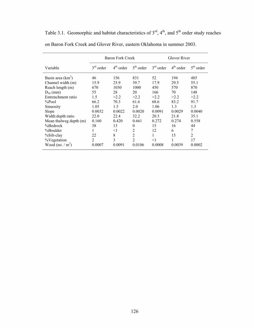
Table 3.1. Geomorphic and habitat characteristics of 3rd, 4th, and 5th order study reaches

on Baron Fork Creek and Glover River, eastern Oklahoma in summer 2003.

Baron Fork Creek Glover River

Variable 3rd order 4th order 5th order 3rd order 4th order 5th order

Basin area (km2) 46 156 831 52 194 485 Channel width (m) 15.9 25.9 39.7 17.9 29.5 55.1 Reach length (m) 670 1030 1000 450 570 870 D50 (mm) 55 28 20 166 70 148 Entrenchment ratio 1.5 >2.2 >2.2 >2.2 >2.2 >2.2 %Pool 66.2 70.3 61.6 68.6 83.2 91.7 Sinuosity 1.05 1.5 2.0 1.06 1.3 1.3 Slope 0.0032 0.0022 0.0020 0.0091 0.0029 0.0040 Width:depth ratio 22.0 22.4 32.2 20.3 21.8 35.1 Mean thalweg depth (m) 0.160 0.420 0.661 0.272 0.274 0.558 %Bedrock 38 13 0 15 16 44 %Boulder 1 <1 2 12 6 7 %Silt-clay 22 8 2 1 15 2 %Vegetation 2 3 2 <1 1 17 Wood (no. / m2) 0.0007 0.0091 0.0106 0.0008 0.0039 0.0002

126

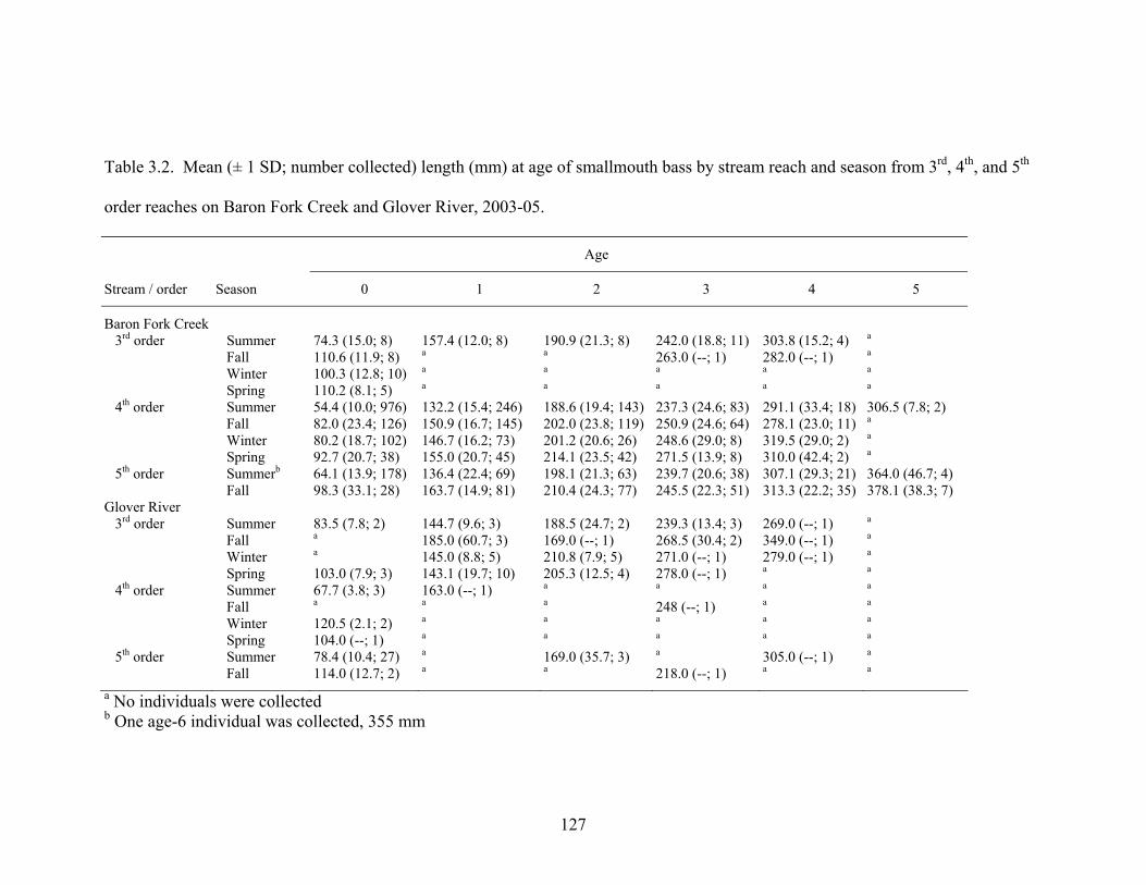
Table 3.2. Mean (± 1 SD; number collected) length (mm) at age of smallmouth bass by stream reach and season from 3rd, 4th, and 5th

order reaches on Baron Fork Creek and Glover River, 2003-05.

Age

Stream / order Season 0 1 2 3 4 5

Baron Fork Creek 3rd order Summer 74.3 (15.0; 8) 157.4 (12.0; 8) 190.9 (21.3; 8) 242.0 (18.8; 11) 303.8 (15.2; 4) a

Fall 110.6 (11.9; 8) a a 263.0 (--; 1) 282.0 (--; 1) a

Winter 100.3 (12.8; 10) a a a a a

Spring 110.2 (8.1; 5) a a a a a

4th order Summer 54.4 (10.0; 976) 132.2 (15.4; 246) 188.6 (19.4; 143) 237.3 (24.6; 83) 291.1 (33.4; 18) 306.5 (7.8; 2) Fall 82.0 (23.4; 126) 150.9 (16.7; 145) 202.0 (23.8; 119) 250.9 (24.6; 64) 278.1 (23.0; 11) a

Winter 80.2 (18.7; 102) 146.7 (16.2; 73) 201.2 (20.6; 26) 248.6 (29.0; 8) 319.5 (29.0; 2) a

Spring 92.7 (20.7; 38) 155.0 (20.7; 45) 214.1 (23.5; 42) 271.5 (13.9; 8) 310.0 (42.4; 2) a

5th order Summerb 64.1 (13.9; 178) 136.4 (22.4; 69) 198.1 (21.3; 63) 239.7 (20.6; 38) 307.1 (29.3; 21) 364.0 (46.7; 4) Fall 98.3 (33.1; 28) 163.7 (14.9; 81) 210.4 (24.3; 77) 245.5 (22.3; 51) 313.3 (22.2; 35) 378.1 (38.3; 7) Glover River 3rd order Summer 83.5 (7.8; 2) 144.7 (9.6; 3) 188.5 (24.7; 2) 239.3 (13.4; 3) 269.0 (--; 1) a

Fall a 185.0 (60.7; 3) 169.0 (--; 1) 268.5 (30.4; 2) 349.0 (--; 1) a

Winter a 145.0 (8.8; 5) 210.8 (7.9; 5) 271.0 (--; 1) 279.0 (--; 1) a

Spring 103.0 (7.9; 3) 143.1 (19.7; 10) 205.3 (12.5; 4) 278.0 (--; 1) a a

4th order Summer 67.7 (3.8; 3) 163.0 (--; 1) a a a a

Fall a a a 248 (--; 1) a a

Winter 120.5 (2.1; 2) a a a a a

Spring 104.0 (--; 1) a a a a a

5th order Summer 78.4 (10.4; 27) a 169.0 (35.7; 3) a 305.0 (--; 1) a

Fall 114.0 (12.7; 2) a a 218.0 (--; 1) a a

a No individuals were collected b One age-6 individual was collected, 355 mm

127

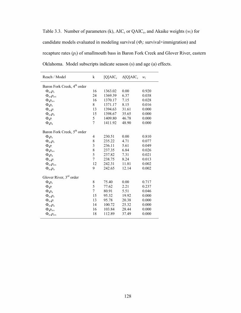
Table 3.3. Number of parameters (k), AICc or QAICc, and Akaike weights (wi) for

candidate models evaluated in modeling survival (Фi: survival×immigration) and

recapture rates (pi) of smallmouth bass in Baron Fork Creek and Glover River, eastern

Oklahoma. Model subscripts indicate season (s) and age (a) effects.

Reach / Model k [Q]AICc ∆[Q]AICc wi

Baron Fork Creek, 4th order Фa·sps 16 1363.02 0.00 0.920 Фa·spa·s 24 1369.39 6.37 0.038 Фspa·s 16 1370.17 7.15 0.028 Фsps 8 1371.17 8.15 0.016 Фa·sp. 13 1394.63 31.61 0.000 Фa·spa 15 1398.67 35.65 0.000 Фsp. 5 1409.80 46.78 0.000 Фspa 7 1411.92 48.90 0.000 Baron Fork Creek, 5th order Фsps 4 230.51 0.00 0.810 Фa·sps 8 235.22 4.71 0.077 Фsp. 3 236.11 5.61 0.049 Фspa·s 8 237.35 6.84 0.026 Фspa 5 237.82 7.31 0.021 Фa·sp. 7 238.75 8.24 0.013 Фa·spa·s 12 242.31 11.81 0.002 Фa·spa 9 242.65 12.14 0.002 Glover River, 3rd order Фsps 8 75.40 0.00 0.717 Фsp. 5 77.62 2.21 0.237 Фspa 7 80.91 5.51 0.046 Фa·sps 15 95.32 19.92 0.000 Фa·sp. 13 95.78 20.38 0.000 Фa·spa 14 100.72 25.32 0.000 Фspa·s 16 103.84 28.44 0.000 Фa·spa·s 18 112.89 37.49 0.000

128

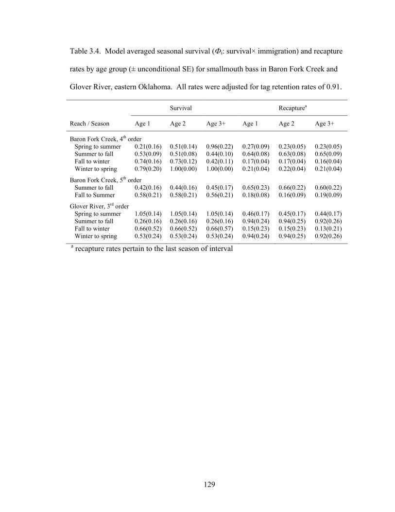
Table 3.4. Model averaged seasonal survival (Фi: survival× immigration) and recapture

rates by age group (± unconditional SE) for smallmouth bass in Baron Fork Creek and

Glover River, eastern Oklahoma. All rates were adjusted for tag retention rates of 0.91.

Survival Recapturea

Reach / Season Age 1 Age 2 Age 3+ Age 1 Age 2 Age 3+

Baron Fork Creek, 4th order Spring to summer 0.21(0.16) 0.51(0.14) 0.96(0.22) 0.27(0.09) 0.23(0.05) 0.23(0.05) Summer to fall 0.53(0.09) 0.51(0.08) 0.44(0.10) 0.64(0.08) 0.63(0.08) 0.65(0.09) Fall to winter 0.74(0.16) 0.73(0.12) 0.42(0.11) 0.17(0.04) 0.17(0.04) 0.16(0.04) Winter to spring 0.79(0.20) 1.00(0.00) 1.00(0.00) 0.21(0.04) 0.22(0.04) 0.21(0.04)

Baron Fork Creek, 5th order

Summer to fall 0.42(0.16) 0.44(0.16) 0.45(0.17) 0.65(0.23) 0.66(0.22) 0.60(0.22) Fall to Summer 0.58(0.21) 0.58(0.21) 0.56(0.21) 0.18(0.08) 0.16(0.09) 0.19(0.09)

Glover River, 3rd order

Spring to summer 1.05(0.14) 1.05(0.14) 1.05(0.14) 0.46(0.17) 0.45(0.17) 0.44(0.17) Summer to fall 0.26(0.16) 0.26(0.16) 0.26(0.16) 0.94(0.24) 0.94(0.25) 0.92(0.26) Fall to winter 0.66(0.52) 0.66(0.52) 0.66(0.57) 0.15(0.23) 0.15(0.23) 0.13(0.21) Winter to spring 0.53(0.24) 0.53(0.24) 0.53(0.24) 0.94(0.24) 0.94(0.25) 0.92(0.26) a recapture rates pertain to the last season of interval

129

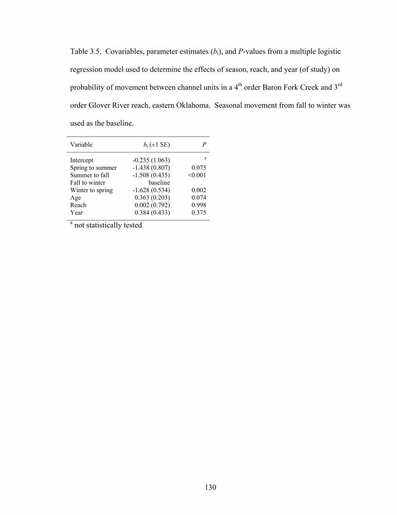
Table 3.5. Covariables, parameter estimates (bi), and P-values from a multiple logistic

regression model used to determine the effects of season, reach, and year (of study) on

probability of movement between channel units in a 4th order Baron Fork Creek and 3rd

order Glover River reach, eastern Oklahoma. Seasonal movement from fall to winter was

used as the baseline.

Variable bi (±1 SE) P

Intercept -0.235 (1.063) a

Spring to summer -1.438 (0.807) 0.075 Summer to fall -1.508 (0.435) <0.001 Fall to winter baseline Winter to spring -1.628 (0.534) 0.002 Age 0.363 (0.203) 0.074 Reach 0.002 (0.792) 0.998 Year 0.384 (0.433) 0.375 a not statistically tested

130

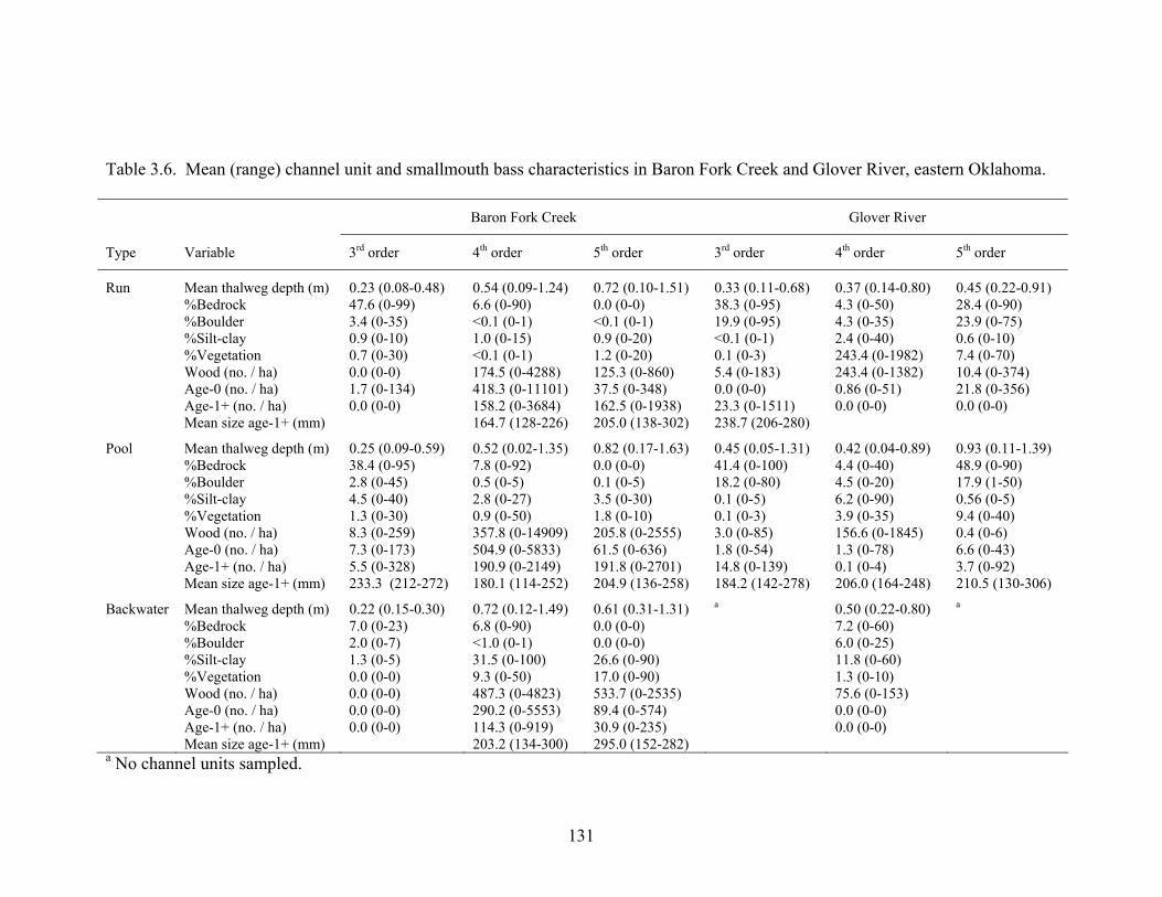
Table 3.6. Mean (range) channel unit and smallmouth bass characteristics in Baron Fork Creek and Glover River, eastern Oklahoma.

Baron Fork Creek Glover River

Type Variable 3rd order 4th order 5th order 3rd order 4th order 5th order

Run Mean thalweg depth (m) 0.23 (0.08-0.48) 0.54 (0.09-1.24) 0.72 (0.10-1.51) 0.33 (0.11-0.68) 0.37 (0.14-0.80) 0.45 (0.22-0.91) %Bedrock 47.6 (0-99) 6.6 (0-90) 0.0 (0-0) 38.3 (0-95) 4.3 (0-50) 28.4 (0-90) %Boulder 3.4 (0-35) <0.1 (0-1) <0.1 (0-1) 19.9 (0-95) 4.3 (0-35) 23.9 (0-75) %Silt-clay 0.9 (0-10) 1.0 (0-15) 0.9 (0-20) <0.1 (0-1) 2.4 (0-40) 0.6 (0-10) %Vegetation 0.7 (0-30) <0.1 (0-1) 1.2 (0-20) 0.1 (0-3) 243.4 (0-1982) 7.4 (0-70) Wood (no. / ha) 0.0 (0-0) 174.5 (0-4288) 125.3 (0-860) 5.4 (0-183) 243.4 (0-1382) 10.4 (0-374) Age-0 (no. / ha) 1.7 (0-134) 418.3 (0-11101) 37.5 (0-348) 0.0 (0-0) 0.86 (0-51) 21.8 (0-356) Age-1+ (no. / ha) 0.0 (0-0) 158.2 (0-3684) 162.5 (0-1938) 23.3 (0-1511) 0.0 (0-0) 0.0 (0-0) Mean size age-1+ (mm) 164.7 (128-226) 205.0 (138-302) 238.7 (206-280)

Pool Mean thalweg depth (m) 0.25 (0.09-0.59) 0.52 (0.02-1.35) 0.82 (0.17-1.63) 0.45 (0.05-1.31) 0.42 (0.04-0.89) 0.93 (0.11-1.39) %Bedrock 38.4 (0-95) 7.8 (0-92) 0.0 (0-0) 41.4 (0-100) 4.4 (0-40) 48.9 (0-90) %Boulder 2.8 (0-45) 0.5 (0-5) 0.1 (0-5) 18.2 (0-80) 4.5 (0-20) 17.9 (1-50) %Silt-clay 4.5 (0-40) 2.8 (0-27) 3.5 (0-30) 0.1 (0-5) 6.2 (0-90) 0.56 (0-5) %Vegetation 1.3 (0-30) 0.9 (0-50) 1.8 (0-10) 0.1 (0-3) 3.9 (0-35) 9.4 (0-40) Wood (no. / ha) 8.3 (0-259) 357.8 (0-14909) 205.8 (0-2555) 3.0 (0-85) 156.6 (0-1845) 0.4 (0-6) Age-0 (no. / ha) 7.3 (0-173) 504.9 (0-5833) 61.5 (0-636) 1.8 (0-54) 1.3 (0-78) 6.6 (0-43) Age-1+ (no. / ha) 5.5 (0-328) 190.9 (0-2149) 191.8 (0-2701) 14.8 (0-139) 0.1 (0-4) 3.7 (0-92) Mean size age-1+ (mm) 233.3 (212-272) 180.1 (114-252) 204.9 (136-258) 184.2 (142-278) 206.0 (164-248) 210.5 (130-306)

Backwater Mean thalweg depth (m) 0.22 (0.15-0.30) 0.72 (0.12-1.49) 0.61 (0.31-1.31) a 0.50 (0.22-0.80) a

%Bedrock 7.0 (0-23) 6.8 (0-90) 0.0 (0-0) 7.2 (0-60) %Boulder 2.0 (0-7) <1.0 (0-1) 0.0 (0-0) 6.0 (0-25) %Silt-clay 1.3 (0-5) 31.5 (0-100) 26.6 (0-90) 11.8 (0-60) %Vegetation 0.0 (0-0) 9.3 (0-50) 17.0 (0-90) 1.3 (0-10) Wood (no. / ha) 0.0 (0-0) 487.3 (0-4823) 533.7 (0-2535) 75.6 (0-153) Age-0 (no. / ha) 0.0 (0-0) 290.2 (0-5553) 89.4 (0-574) 0.0 (0-0) Age-1+ (no. / ha) 0.0 (0-0) 114.3 (0-919) 30.9 (0-235) 0.0 (0-0) Mean size age-1+ (mm) 203.2 (134-300) 295.0 (152-282) a No channel units sampled.

131

Figure 3.1. Conceptual model of fish life cycles emphasizing habitat use and movement

(adapted from Schlosser 1991; 1995).

Figure 3.2. Study reaches on Baron Fork Creek and Glover River, eastern Oklahoma.

Reaches on 3rd, 4th, and 5th order stream segments were selected on each stream, and

sampled seasonally from July 2003 to August 2005.

Figure 3.3. Mean (± 1 SD) monthly water temperatures in 3rd (black), 4th (gray), and 5th

(dashed) order reaches of Baron Fork Creek (A) and Glover River (B), eastern Oklahoma

from July 2003 to July 2005.

Figure 3.4. Mean daily streamflow at 3rd, 4th, and 5th order reaches of Baron Fork Creek

(A) and Glover River (B), eastern Oklahoma from July 2003 to July 2004. Provisional

data from USGS gauging stations after September 2004 were excluded.

Figure 3.5. Mean relative growth rate (± SE) in length of smallmouth bass by season in

Baron Fork Creek and Glover River, eastern Oklahoma. Different letters indicate

significant differences among seasons.

Figure 3.6. Mean relative weights (± SE) of smallmouth bass by stream and stream order

(top), and by season (bottom) in Baron Fork Creek and Glover River, eastern Oklahoma.

Asterisk indicates differences in relative weights between streams at a stream order.

Linear contrasts suggested a linear decrease in relative weight with stream order in Baron

132

Fork Creek (F1, 1227 = 68.74; P < 0.001); no quadratic trend was evident (F1, 1226 = 2.16; P

= 0.142). No trend was observed for the Glover River (linear: F1, 1226 = 1.21; P = 0.272).

Seasons where relative weights differed are indicated by different letters.

Figure 3.7. Densities of age-1+ smallmouth bass in Baron Fork Creek, eastern Oklahoma

from July 2003 to July 2005. Non-contiguous channel units indicate dry stream segments

during low flow periods.

Figure 3.8. Location of temperature loggers upstream, downstream, at the outlet, and in a

backwater in a 4th order reach of Baron Fork Creek, eastern Oklahoma.

Figure 3.9. Winter and summer temperatures upstream, downstream, at the outlet, and at

the back of a backwater habitat in the 4th order reach of Baron Fork Creek, eastern

Oklahoma. Temperature loggers that malfunctioned or that were lost to floods resulted in

non-continuous temperature records for some locations.

Figure 3.10. Regression tree analysis of effects stream, stream order, season, and channel

unit habitat on age-0 smallmouth bass densities (no / ha) in 849 channel units from three

reaches each in Baron Fork Creek and Glover River, eastern Oklahoma. Mean densities

per node are given, with sample sizes in parentheses. Observations with variable values

less than or equal to node value split to the left, and values greater than split right.

Terminal nodes are oval. 10-fold cross-validated relative error was 0.797.

133

Figure 3.11. Regression tree analysis of effects stream, stream order, season, and channel

unit habitat on age-1+ smallmouth bass densities (no / ha) in 849 channel units from three

reaches each in Baron Fork Creek and Glover River, eastern Oklahoma. Mean densities

per node are given, with sample sizes in parentheses. Observations with variable values

less than or equal to node value split to the left, and values greater than split right.

Terminal nodes are oval. 10-fold cross-validated relative error was 0.724.

Figure 3.12. Regression tree analysis of effects stream, stream order, season, and channel

unit habitat on size of age-1+ smallmouth bass in 156 channel units from three reaches

each in Baron Fork Creek and Glover River, eastern Oklahoma. Mean lengths (mm) per

node are given, with sample sizes in parentheses. Observations with variable values less

than or equal to node value split to the left, and values greater than split right. Terminal

nodes are oval. 10-fold cross-validated relative error was 0.856.

134

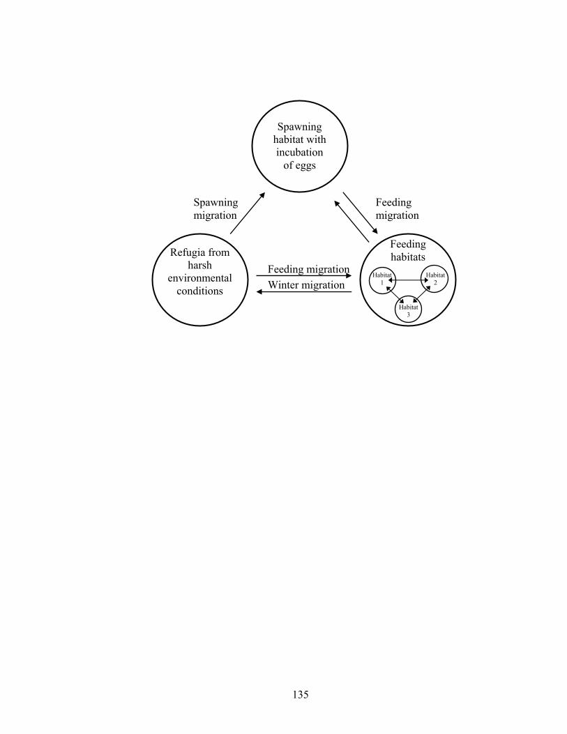
Spawning habitat with incubation

of eggs

Refugia from harsh

environmental conditions

Feeding habitats

Winter migration Feeding migration

Spawning migration

Feeding migration

Habitat 1

Habitat 2

Habitat 3

135

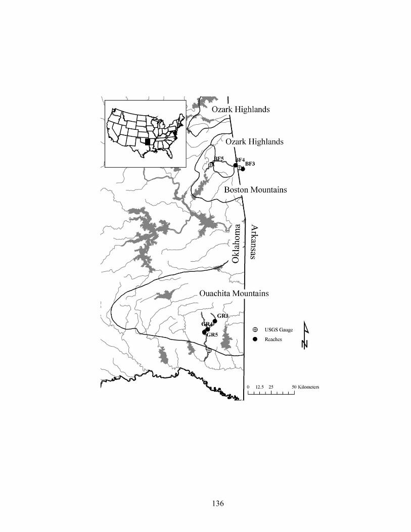
136

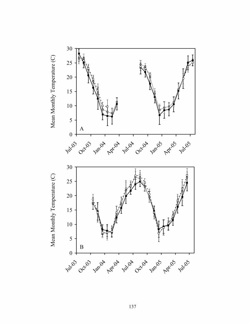
0

5

10

15

20

25

30

Jul-03

Oct-03

Jan-04

Apr-04

Jul-04

Oct-04

Jan-05

Apr-05

Jul-05

Mea

n M

onth

ly T

empe

ratu

re (C

)

A

0

5

10

15

20

25

30

Jul-03

Oct-03

Jan-04

Apr-04

Jul-04

Oct-04

Jan-05

Apr-05

Jul-05

Mea

n M

onth

ly T

empe

ratu

re (C

)

B

137

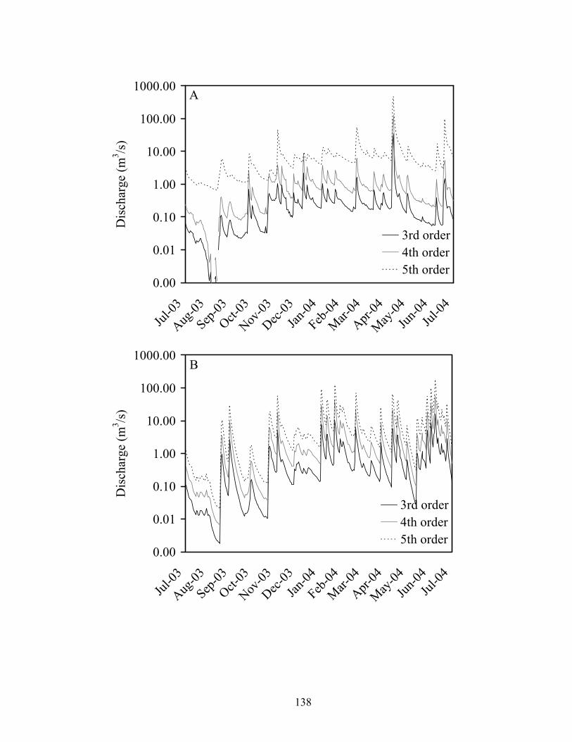
0.00

0.01

0.10

1.00

10.00

100.00

1000.00

Jul-03

Aug-03

Sep-03

Oct-03

Nov-03

Dec-03

Jan-04

Feb-04

Mar-04

Apr-04

May-04

Jun-04

Jul-04

Dis

char

ge (m

3 /s)

3rd order4th order5th order

A

0.00

0.01

0.10

1.00

10.00

100.00

1000.00

Jul-03

Aug-03

Sep-03

Oct-03

Nov-03

Dec-03

Jan-04

Feb-04

Mar-04

Apr-04

May-04

Jun-04

Jul-04

Dis

char

ge (m

3 /s)

3rd order4th order5th order

B

138

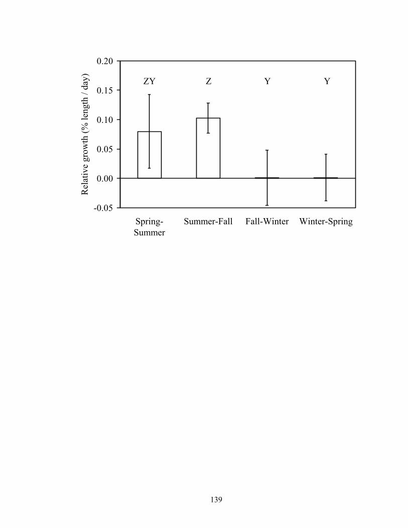
-0.05

0.00

0.05

0.10

0.15

0.20

Spring-Summer

Summer-Fall Fall-Winter Winter-Spring

Rel

ativ

e gr

owth

(% le

ngth

/ da

y) ZY Z Y Y

139

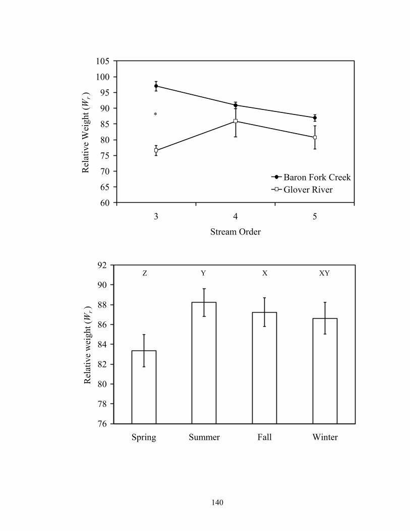
60

65

70

75

80

85

90

95

100

105

3 4 5

Stream Order

Rel

ativ

e W

eigh

t (W

r)

Baron Fork CreekGlover River

*

76

78

80

82

84

86

88

90

92

Spring Summer Fall Winter

Rel

ativ

e w

eigh

t (W

r)

Z Y X XY

140

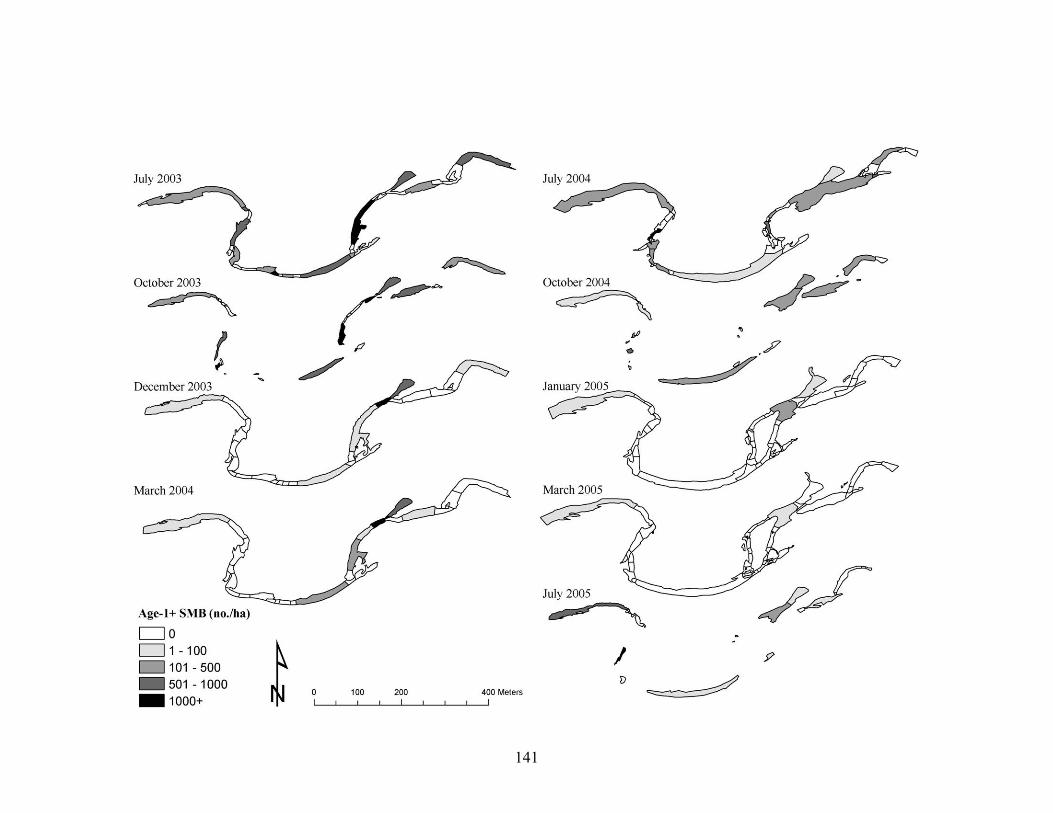
141

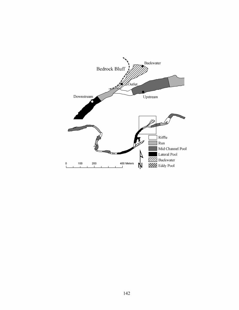
142

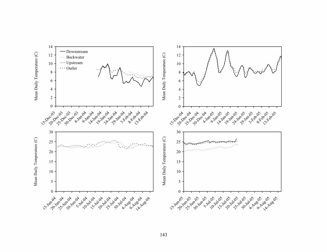
143

0

2

4

6

8

10

12

14

15-D

ec-03

20-D

ec-03

25-D

ec-03

30-D

ec-03

4-Jan

-049-J

an-04

14-Ja

n-04

19-Ja

n-04

24-Ja

n-04

29-Ja

n-04

3-Feb

-048-F

eb-04

13-Feb

-04

Mea

n D

aily

Tem

pera

ture

(C) Downstream

BackwaterUpstreamOutlet

0

5

10

15

20

25

30

15-Ju

n-05

20-Ju

n-05

25-Ju

n-05

30-Ju

n-05

5-Jul-

0510

-Jul-0

515

-Jul-0

520

-Jul-0

525

-Jul-0

530

-Jul-0

54-A

ug-05

9-Aug

-0514

-Aug

-05

Mea

n D

aily

Tem

pera

ture

(C)

0

5

10

15

20

25

30

15-Ju

n-04

20-Ju

n-04

25-Ju

n-04

30-Ju

n-04

5-Jul-

0410

-Jul-0

415

-Jul-0

420

-Jul-0

425

-Jul-0

430

-Jul-0

44-A

ug-04

9-Aug

-0414

-Aug

-04

Mea

n D

aily

Tem

pera

ture

(C)

0

2

4

6

8

10

12

14

15-D

ec-04

20-D

ec-04

25-D

ec-04

30-D

ec-04

4-Jan

-059-J

an-05

14-Ja

n-05

19-Ja

n-05

24-Ja

n-05

29-Ja

n-05

3-Feb

-058-F

eb-05

13-Feb

-05

Mea

n D

aily

Tem

pera

ture

(C)

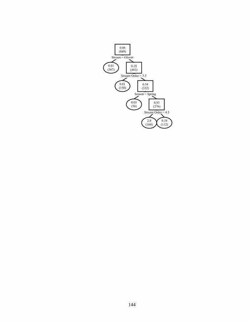
0.06 (849)

0.18 (482)

0.01 (150)

0.03 (56)

Stream Order = 3.5

0.54 (332)

0.93 (276)

0.18 (112)

2.8 (164)

0.01 (367)

Season = Spring

Stream Order = 4.5

Stream = Glover

144

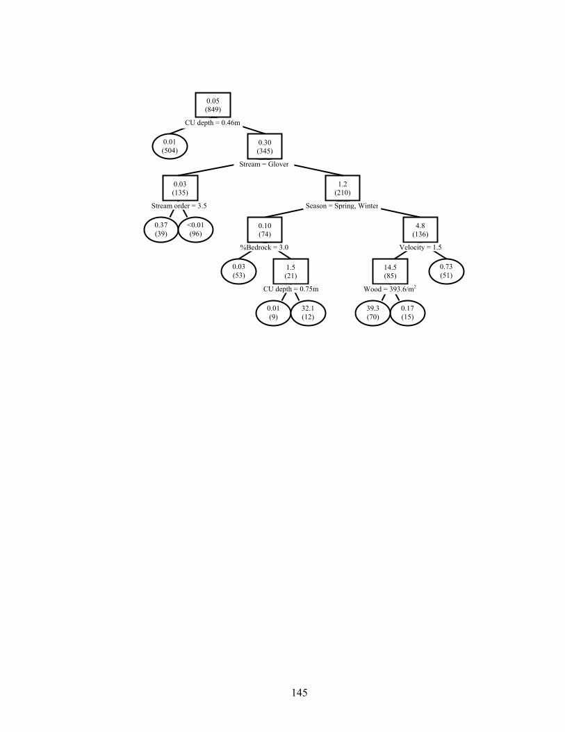
0.30 (345)

0.05 (849)

4.8 (136)

1.2 (210)

0.03 (135)

1.5 (21)

14.5 (85)

0.03 (53)

0.01 (9)

32.1 (12)

Stream = Glover

Season = Spring, Winter

%Bedrock = 3.0

CU depth = 0.75m

0.73 (51)

0.10 (74)

0.17 (15)

39.3 (70)

Velocity = 1.5

Wood = 393.6/m2

0.01 (504)

0.37 (39)

<0.01 (96)

Stream order = 3.5

CU depth = 0.46m

145

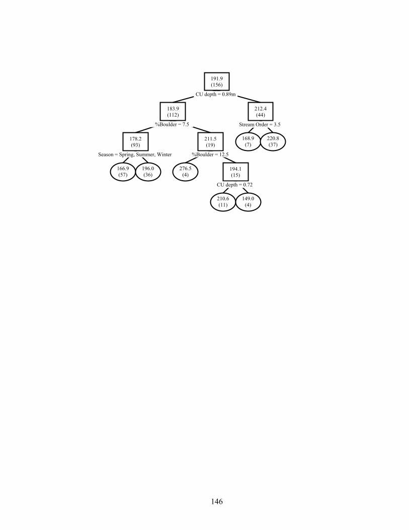
191.9 (156)

212.4 (44)

276.5 (4)

166.9 (57)

196.0 (36)

183.9 (112)

178.2 (93)

211.5 (19)

168.9 (7)

%Boulder = 7.5

220.8 (37)

Season = Spring, Summer, Winter

CU depth = 0.89m

Stream Order = 3.5

194.1 (15)

210.6 (11)

149.0 (4)

CU depth = 0.72

%Boulder = 12.5

146

Appendix 3.A. Snorkeling and electrofishing methods for estimating smallmouth bass

abundance.

Methods

Mark-recapture data were used to develop a 3-pass capture probability model to estimate

smallmouth bass abundance in channel units. In 24 channel units in two eastern

Oklahoma streams, smallmouth bass were collected, marked, and returned. Habitat

variables measured were: mean thalweg depth (m), %bedrock, %silt-clay, wood density

(no./m2). After a recovery period, three electrofishing passes were made to recapture

individuals. Capture probability was estimated using multiple logistic regression using

SAS software, version 9.1 (SAS Institute Inc., Cary, North Carolina) with fish size (< and

≥100 mm), electrofishing power (µS/cm3), and all habitat variables as potential

explanatory variables: 110 ....)]ˆˆexp(1[ˆ −−−+= ixp ββ

All combinations of explanatory variables, including fish size×depth, depth×%bedrock

and depth×%silt-clay interactions, were evaluated using model selection and averaging

methods. Abundance estimates were obtained by correcting number of individuals

collected (C) by model averaged, predicted capture probability, . pCN ˆ/ˆ =

Results

All habitat variables, except mean thalweg depth×%silt-clay interaction, were included in

at least one candidate model (Table 3.A.1). Fish size and mean thalweg depth, and their

interaction, had the largest effect on capture probabilities (Table 3.A.2). Abundance

estimates from the 3-pass model, when compared to known abundances using linear

regression, were precise (r2 = 0.881) and unbiased (bi = 1, P = 0.462).

147

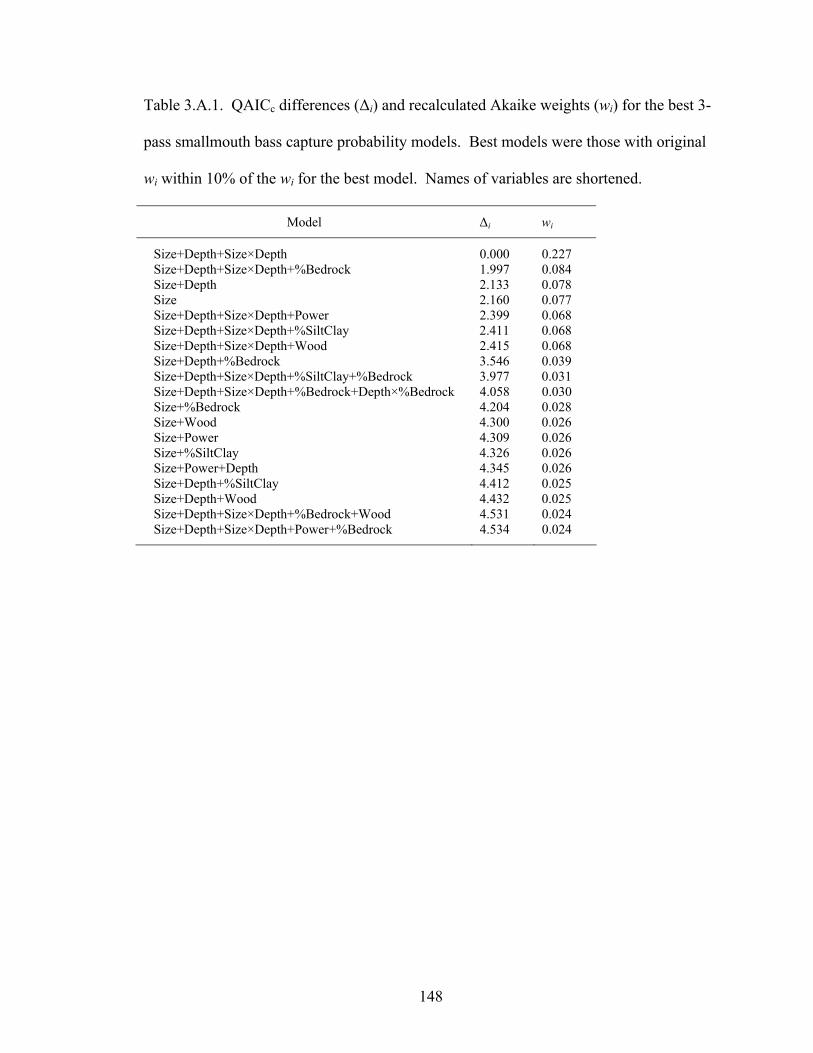
Table 3.A.1. QAICc differences (∆i) and recalculated Akaike weights (wi) for the best 3-

pass smallmouth bass capture probability models. Best models were those with original

wi within 10% of the wi for the best model. Names of variables are shortened.

Model ∆i wi

Size+Depth+Size×Depth 0.000 0.227 Size+Depth+Size×Depth+%Bedrock 1.997 0.084 Size+Depth 2.133 0.078 Size 2.160 0.077 Size+Depth+Size×Depth+Power 2.399 0.068 Size+Depth+Size×Depth+%SiltClay 2.411 0.068 Size+Depth+Size×Depth+Wood 2.415 0.068 Size+Depth+%Bedrock 3.546 0.039 Size+Depth+Size×Depth+%SiltClay+%Bedrock 3.977 0.031 Size+Depth+Size×Depth+%Bedrock+Depth×%Bedrock 4.058 0.030 Size+%Bedrock 4.204 0.028 Size+Wood 4.300 0.026 Size+Power 4.309 0.026 Size+%SiltClay 4.326 0.026 Size+Power+Depth 4.345 0.026 Size+Depth+%SiltClay 4.412 0.025 Size+Depth+Wood 4.432 0.025 Size+Depth+Size×Depth+%Bedrock+Wood 4.531 0.024 Size+Depth+Size×Depth+Power+%Bedrock 4.534 0.024

148

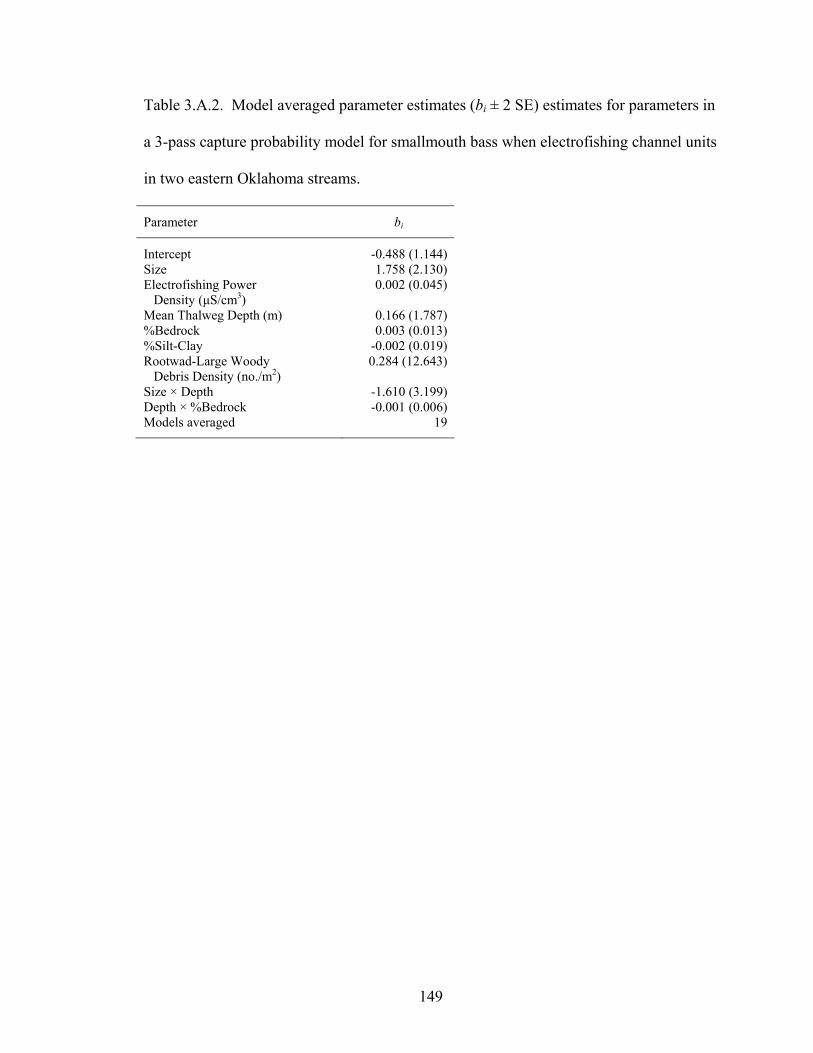
Table 3.A.2. Model averaged parameter estimates (bi ± 2 SE) estimates for parameters in

a 3-pass capture probability model for smallmouth bass when electrofishing channel units

in two eastern Oklahoma streams.

Parameter bi

Intercept -0.488 (1.144) Size 1.758 (2.130) Electrofishing Power Density (µS/cm3)

0.002 (0.045)

Mean Thalweg Depth (m) 0.166 (1.787) %Bedrock 0.003 (0.013) %Silt-Clay -0.002 (0.019) Rootwad-Large Woody Debris Density (no./m2)

0.284 (12.643)

Size × Depth -1.610 (3.199) Depth × %Bedrock -0.001 (0.006) Models averaged 19

149

CHAPTER 4

NESTING CHRONOLOGY, NEST SITE SELECTION, AND NEST SUCCESS OF

SMALLMOUTH BASS DURING BENIGN STREAMFLOW CONDITIONS

150

Abstract

We documented the nesting chronology, nest site selection, and nest success of

smallmouth bass Micropterus dolomieu in an upstream (4th order) and downstream (5th

order) reach of Baron Fork Creek, Oklahoma. Males started nesting in mid-April when

water temperatures increased to 16.9°C upstream, and in late-April when temperatures

increased to 16.2°C downstream. Streamflows were low (77% upstream to 82%

downstream of mean April streamflow, and 12 and 18% of mean June streamflow; 47

and 55 years of record), and decreased throughout the spawning period. Larger males

nested first upstream, as has been observed in other populations, but not downstream.

Upstream, 62 of 153 nests developed to swim-up stage. Downstream, 31 of 73 nests

developed to swim-up. Nesting densities upstream (147 / km) and downstream (100 /

km) were both higher than any densities previously reported. Males selected nest sites

with intermediate water depths, low water velocity, and near cover, behavior that is

typical of smallmouth bass. Documented nest failures resulted from human disturbance,

angling, and longear sunfish predation. Logistic exposure models showed that water

velocity at the nest was negatively related and length of the guarding male was positively

related to nest success upstream. Male length and number of degree days were both

positively related to nest success downstream. Our results, and those of other studies,

suggest that biological factors account for most nest failures during benign (stable, low

flow) streamflow conditions, whereas nest failures attributed to substrate mobility or nest

abandonment dominate when harsh streamflow conditions (spring floods) coincide with

the spawning season.

151

Introduction

The spawning behaviors of smallmouth bass Micropterus dolomieu in streams are well

documented. Spawning begins in April or May when water temperature rise to ~15°C

(Wrenn 1984; Graham and Orth 1986). Male smallmouth bass build circular depressions

for nests in areas with gravel or larger substrates and adjacent to cover, with the extent of

cover use changing among years (Pflieger 1966; Reynolds and O'Bara 1991). After nest

construction, hours to weeks may pass before a male coaxes a female to deposit eggs in

the nest (Pflieger 1966). Males will guard the nest until nest failure or fry swim up off

the nest and disperse about two weeks after egg deposition.

The ability of a male smallmouth bass to raise a successful brood in streams is

dependent on both physical and biological factors. Proximity of the nest to cover,

streamflow, water temperature, and male size determine nest success, with larger males

being more successful (Reynolds and O'Bara 1991; Lukas and Orth 1995). Larger males

typically spawn earlier than smaller males (Ridgway et al. 1991; Lukas and Orth 1995),

but they may lose broods during flood events early in the spawning period (Lukas and

Orth 1995). Other biological factors such as nest predation or fungus development also

affect nest success (Reynolds and O'Bara 1991; Lukas and Orth 1995).

Oklahoma has two genetically divergent, peripheral populations of native

smallmouth bass, the Neosho smallmouth bass in the Ozark Highlands and Boston

Mountains ecoregions (Omernik 1987) in the northeast and the Ouachita smallmouth bass

in the Ouachita Mountains of the southeast (MacCrimmon and Robbins 1975; Stark and

Echelle 1998). Coincidentally, smallmouth bass in eastern Oklahoma show demographic

differences from other populations in the native range of the species; they have higher

152

mortality rates and are generally shorter lived (Balkenbush and Fisher 2001). Whether

these demographic differences are genetically or habitat related is unknown. Regardless,

studies on nesting habits of smallmouth bass in eastern Oklahoma are lacking, and it is

unknown whether the nesting habits typically observed in smallmouth bass transfer to

these peripheral and divergent populations.

Our goal was to document the spawning of smallmouth bass in Baron Fork Creek,

Oklahoma. Specifically, we documented the chronology of Neosho smallmouth bass

spawning, evaluated microhabitats selected by nesting males, and assessed physical and

biological factors influencing nest success.

Study sites

Our study occurred in two reaches of Baron Fork Creek, Oklahoma (Figure 4.1). Baron

Fork Creek originates in northwest Arkansas and flows west-southwest through the

Ozark Highlands and Boston Mountains ecoregions (Omernik 1987; Woods et al. 2005)

and into the Illinois River system at Lake Tenkiller in northeast Oklahoma. The drainage

area of Baron Fork Creek is 936 km2 and consists mostly of forest and pastureland

(Balkenbush and Fisher 2001). The upstream reach, hereafter referred to as Baron, is

located in Adair County near the Arkansas state line, 35°54’53.64”N, 94°32’23.76”W.

The reach was 1038.8 m in length, with a slope of 0.22%. Substrates consisted mostly of

pebbles (D50 = 28.2 mm). The downstream reach, Eldon, is in Cherokee County,

35°56’5.10”N, 94°49’46.17”W. The reach length was 728.2 m, and had a slope of

0.20%. Substrates were dominated by pebbles (D50 = 20.0 mm). Both reaches were

153

characterized as low gradient, meandering with point bars, riffle-pool morphology, and

alluvial with wide floodplains (Rosgen 1994).

Methods

Nesting chronology

We started monitoring each reach for spawning activity in April 2005. Sites were

visited weekly until spawning activity was observed from the streambank. Each reach

was surveyed completely after spawning activity was detected, usually every 2-5 days by

one or two snorkelers. New nests were marked on their downstream side with a rock

containing a unique number, and an identically numbered flag was placed on the

streambank perpendicular to each nest to facilitate relocation. The total length of the

guarding male was estimated by underwater observation; snorkelers were trained on 100

and 300 mm models of bass. A subset of males was angled from the nest and measured

for total length. A relation between estimated and actual lengths (Actual Length =

43.18+Estimated Length×0.896; r2 = 0.803) was used to correct for estimated length bias

when an actual length was not available.

To document size trends in spawning chronology we evaluated the relation

between the log10 number of degree days (sum of mean daily temperature >10°C) and

log10 male total length using linear regression (Lukas and Orth 1995). Only the first

nesting attempts of males that knowingly renested were analyzed. Age frequencies of

spawning males were estimated using an age-length key (DeVries and Frie 1996) with

2.5 cm length groups developed using aged individuals sampled in spring and summer

2003 to 2005 from both study reaches.

154

Nest site selection

Microhabitat characteristics associated with each nest were measured to estimate

habitat selection by nesting males. Characteristics measured were: mean velocity (m/s;

0.6 of water depth); velocity at the nest (0.04 m above substrate); water depth (m); nest

and surrounding dominant substrate, classified visually using the modified Wentworth

scale (Bain 1999) and coded using rank of size (bedrock = 0, silt/clay = 1, sand = 2,

gravel = 3, pebble = 4, cobble = 5, boulder = 6); and number of submerged cover

structures within 1 and 2 m of the nest. Large woody debris (≥ 4 m in length and 10 cm

in diameter), rootwads, boulders, aquatic vegetation, and undercut banks were considered

cover.

We compared habitat use by nesting smallmouth bass males versus available

habitat to determine selected microhabitat characteristics. Habitat availability was

measured (same variables as above) at randomly selected points within the reach.

Approximately midway through the spawning period, each reach was mapped at the

channel unit spatial scale (Hawkins et al. 1993) using a Trimble GeoXT global

positioning system (GPS) receiver (Dauwalter et al. 2006). Reach maps were

downloaded into a geographic information system and 300 random points were selected

within reach boundaries. Existing microhabitat data from the Baron reach suggested that

a sample size of 300 was needed to estimate water depth and velocity means with ≤20%

precision (D. C. Dauwalter, unpublished data). Each data layer of random points was

uploaded into a GPS receiver that was used to navigate to within 0.5 m of each random

point.

155

We assessed microhabitat selection by nesting smallmouth bass by using a

resource selection function (Manly et al. 1993). The resource selection function equated

to a multiple logistic regression (Hosmer and Lemeshow 2000) because our data were

spatially continuous. Multiple logistic regression (PROC GENMOD; SAS Institute, Inc.,

Version 9, Cary, NC) was used to predict whether a sample was from a nest location or

random point by using microhabitat variables. The model used microhabitat variables to

predict relative probabilities of use by nesting smallmouth bass; only relative

probabilities could be determined because both use and availability data were point

samples, and we could not determine the exact proportion of available habitat that was

used (Manly et al. 1993).

All microhabitat variables were evaluated for use in the resource selection

functions for each reach. Pearson correlations were used to identify correlations (r >

0.50) among variables. If needed, one variable from a correlated set was retained in the

global models. Retained microhabitat variables were used to model resource selection

using an information-theoretic framework (Burnham and Anderson 2002). Quadratic

terms for water depth and substrate, and a depth × velocity interaction were also included

in the global models. Lack-of-fit of the global models was assessed using a Hosmer-

Lemeshow test (Hosmer and Lemeshow 2000). All combinations of variables included

in the global models, including an intercept only model, were evaluated, with the

condition that quadratic and interaction terms were only considered in combination with

their constituent variables. Akaike’s Information Criterion corrected for small sample

bias (AICc) was used to quantify parsimony in each model, and Akaike weights (wi) were

computed. Model averaging was conducted only with models having an original wi

156

within 10% of the best model. The recalculated wi for the best subset of models was used

to average parameter estimates from each model; parameters not included in a specific

model were given a value of zero for that model during averaging (Burnham and

Anderson 2002).

Nest success

Each nest was revisited 1 to 7 times to document nest development, success, or

failure. Stage of nest development was recorded during each revisit as: eggs, yolk sac,

black fry, or swim up. Nests were considered successful when 100% of fry had swum up

from the nest. Nests containing zero eggs or fry were considered failures.

We evaluated effects of physical and biological variables on nest success.

Variables evaluated included water depth (m), mean water velocity (m/s), water velocity

at the nest (m/s), abundance of submerged cover within 1 and 2 m (defined as above),

distance to shore (m), degree days (defined as above), mean daily temperature during

incubation (°C), mean discharge during incubation (m3/s), and length of guarding male

(mm). Water temperature was recorded at one location in the middle-third of each reach

with StowAway® Tidbit® temperature loggers (Onset Computer Corporation, Bourne,

Massachusetts). Streamflow data were obtained from United States Geological Survey

(USGS) stream gauges. Data from gauge 07196900 at Dutch Mills, Arkansas were used

for the Baron reach (~7.5 km upstream of reach), and gauge 07197000 at Eldon,

Oklahoma was used for the Eldon reach (~1.5 km downstream from reach). Streamflow

data used were classified as provisional by the USGS.

157

A logistic exposure model was used to evaluate effects of physical and biological

characteristics on nest success. The logistic exposure model extends the typical multiple

logistic regression model to allow for variable exposure periods (time between nest

revisits) in the link function,

iit

t

e xx βββθ

θ+++=

⎟⎟⎟

⎠

⎞

⎜⎜⎜

⎝

⎛

−...

1log 1101

1

where θ is probability of a nest surviving an exposure period, t = the length of the

exposure period, and β = slope coefficients for predictor variables, x (Shaffer 2004).

Variable exposure periods that are not accounted for can bias survival estimates.

Assumptions of the model are that nest success is independent of other nests, and that

daily survival probabilities are homogenous within and among nests. As in multiple

logistic regression, multiple independent variables (physical and biological variables in

this case) can be included in the predictor function.

Information-theory methods again were used to model nest success. One

predictor variable out of a correlated set (r > 0.50) was retained in the global models.

Global models were assessed using a Hosmer-Lemshow test (Hosmer and Lemeshow

2000). All combinations of variables in the global model were evaluated using AICc,

including an intercept-only model, and model selection and averaging proceeded as

described in the previous section (Burnham and Anderson 2002).

158

Results

Nesting chronology

The 2005 nesting period of smallmouth bass in Baron Fork Creek began in mid-

April and lasted through most of June (Figure 4.2). Streamflows were low, and decreased

throughout the spawning period. In April, streamflows were 77 and 82% of mean

monthly streamflows upstream (47 years of record) and downstream (55 years),

respectively. In June, they were 12% upstream and 18% downstream of mean monthly

streamflows. Spawning started earlier and lasted just as long in the Baron reach when

compared to the downstream reach at Eldon. Smallmouth bass nests were first observed

on 17 April at Baron when water temperatures reached 16.9°C. We found four recently

dispersed schools of fry at Eldon during our first extensive snorkeling survey after noting

nest activity on 10 May, and back-calculated dates of egg deposition to 27 April when

water temperatures were 16.2°C. Spawning ceased prior to 18 June at Baron, but we

observed one new nest at Eldon on 18 June during our last survey but did not document

its development. In all, 153 (147 / km) nests attempts were observed at Baron, 3 were

second attempts in the same nest. Seventy-three (100 / km) nest attempts were observed

at Eldon, and 5 were second attempts. We were unable to uniquely identify all

individuals to document all renesting attempts, especially those in different nests.

A size trend in spawning chronology of males was detected for only one of the

two Baron Fork Creek reaches. In the Baron reach, there was a negative but weak

relation; log10 male total length = 2.925 – 0.174·log10 degree days (n = 127, r2 = 0.211, P

< 0.001). The null hypothesis of no relation between degree days and male length in the

Eldon reach was not rejected (n = 65, r2 = 0.027, P = 0.191). Spawning males were

159

mostly represented by age 2, 3, and 4 individuals in the Baron reach, and age 3 and 4

individuals in the Eldon reach (Table 4.1).

Nest site selection

Nests were typically constructed in pool and backwater habitats (Figures 4.3, 4.4)

of low velocity in areas at least 0.24 m in depth (maximum = 1.8 m). Nests located

adjacent to cover typically were associated with woody structure and boulders (Figure

4.5). They were built in areas surrounded by most substrate size classes (Table 4.2), but

97.3% of all nests had pebble substrates, which was the predominant substrate type in

both reaches.

Resource selection functions suggested that smallmouth bass selected nesting

sites in specific microhabitats. In the Baron reach, habitat at 153 nests was compared to

habitat at 294 random points. Six of the 300 random points fell outside of stream

margins during GPS navigation and were omitted. Habitat at 73 nests was compared to

habitat at 297 random points in the Eldon reach. Each nesting attempt was treated as an

observation because we were unable to uniquely identify each individual to document

renesting in new nests. Mean velocity was correlated with nest/bottom velocity (Baron, r

= 0.897; Eldon, r = 0.885), and was excluded from the global model. Amount of cover

within 2 m was correlated with the amount in 1 m (Baron, r = 0.877; Eldon, r = 0.862)

and also was excluded. The global models for the Baron (χ2 = 12.38, df = 8, P = 0.135)

and Eldon (χ2 = 2.49, df = 0.962, P > 0.999) reaches did not show lack of fit. Thirty-one

candidate models were considered for each reach. The global model had the highest

Akaike weight in both reaches, and three other models had weights within 10% of the

160

best (Appendix 4.1). Model averaging of parameters was completed using only the four

best models. Model-averaged parameter estimates for both reaches showed that only

depth, depth quadratic term, and amount of cover within 1 m had parameter estimates

with unconditional (on a specific model) 95% confidence intervals (bi ± 2 SE) that

excluded zero (Table 4.3). Model-averaged relative probabilities of use showed that

smallmouth bass selected nest areas with intermediate water depths and near areas with

cover in both reaches (Figure 4.6). They were not selective for substrate sizes.

Nest success

Of the nesting attempts observed, 62 of 153 developed to swim up in the Baron

reach, and 31 of 73 did so in the Eldon reach. We observed fungus development on most

nests, presumably water mold Saprolegnia parasitica or related species (Knotek and Orth

1998), and nests located in shallow water and reaching an advanced stage typically had

high algal growth as well. The range of fungus coverage on eggs prior to egg hatch was

0 to 100% for each site, and averaged 54.3% at Baron and 26.7% at Eldon. Estimated

time to swim-up was 8 to 19 days, and was less later in the spawning period. No floods

occurred during the spawning period, and most documented nest failures resulted from

longear sunfish Lepomis megalotis predation. On several occasions we observed nest

depredation by a school of longear sunfish. In these instances, the guarding male

smallmouth bass could not defend the nest, and sometimes he did not attempt to do so.

Depredated nests usually contained clean gravel, as all eggs, fungus, and algae (if

present) were consumed, and were easily classified as failed. Three nests in the Baron

reach were physically disturbed: human footprints were observed at two nest locations

161

and motor vehicle tracks at another. Two nests in the Eldon reach were lost to human

disturbance. An angler caught and harvested the male from one nest, and another was

physically disturbed.

Logistic exposure models indicated that only a few of the studied variables affect

nest success. Nesting attempts already at swim up stage (Eldon, n = 6) or disturbed by

humans (see above) were excluded from logistic exposure models. In the Baron reach,

149 nests were analyzed and 62 were successful. In the Eldon reach, 65 nests were

analyzed and 25 were successful (Table 4.4). The amount of cover within 2 m of a nest

was correlated with the amount within 1 m (Baron, r = 0.877; Eldon, r = 0.801), and

mean daily temperature was correlated with number of degree days (Baron, r = 0.936;

Eldon, r = 0.935). We did not include nest substrate in the global models because almost

all nest substrates were pebble. Variables included in the global model for each reach

were water depth, water velocity at the nest, amount of submerged cover within 1 m,

distance to shore, male length, and number of degree days. Male length was only

estimated for 128 nests at Baron and 63 at Eldon because some males were spooked from

the nest during snorkeling surveys or by observers on the streambank. Consequently,

those males were never observed on the nest prior to failure. This reduced sample size

for models containing male length as an independent variable. Global models for the

Baron reach (χ2 = 2.86, df = 8, P = 0.943) and the Eldon reach (χ2 = 0.008, df = 8, P >

0.999) did not show lack of fit. Sixty-four candidate models were considered overall.

Fourteen models had Akaike weights within 10% of the best model for Baron nests, and

16 models were within 10% in the Eldon reach (Appendix 4.2). Six variables plus the

intercept were included in at least one of the best models for the Baron reach. However,

162

only water velocity at the nest and male length had model-averaged parameter estimates

with unconditional 95% confidence intervals that excluded zero. All six variables were

included in at least one of the best models for the Eldon reach also, but only the intercept,

degree days, and male length had approximate 95% confidence intervals that excluded

zero (Table 4.5).

Discussion

Although nesting densities during the 2005 smallmouth-bass spawning season in

Baron Fork Creek were higher than those previously reported, nesting chronology and

microhabitat selection of nest sites in Baron Fork Creek was typical for smallmouth bass,

with slight differences between upstream and downstream reaches. Streamflow

conditions were benign throughout the spawning period, and no nests were lost to

streamflow disturbances as is often found when spring floods coincide with the spawning

season. Most nest failures apparently resulted from nest depredation.

In Baron Fork Creek, spawning was initiated in mid- to late-April when water

temperatures reached 16.2-16.9°C. In Little Saline Creek, Missouri smallmouth bass

spawned from 26 April to 31 May when water temperatures were greater than 15.5°C

(Pflieger 1966). Over a 10-year period in Courtois Creek, Missouri they began spawning

with an abrupt rise in water temperature when daily minimum and maximum were 12.8

and 18.3°C (Pflieger 1975). Studies in Tennessee and Virginia streams reported similar

findings (Reynolds and O'Bara 1991; Lukas and Orth 1995). Graham and Orth (1986)

built a discriminate function model for five stream sites in the New River drainage,

Virginia and West Virginia that suggested mean and maximum daily water temperature,

163

streamflow, and daily accumulation of degree days >15°C were most important in

identifying days when smallmouth bass had spawned. Spawning activity had mostly

ended when we stopped surveying at the end of June. However, on 13 July 2004 we

observed a school of fry in the Baron reach, suggesting sporadic summertime spawning.

We found 100 to 147 nests per stream kilometer in Baron Fork Creek. To our

knowledge, the highest density reported in the literature was 75.3 / km in the Green

River, Tennessee (Table 4.6). It has been suggested that high nesting densities reflect

concentrations of individuals in limited areas of suitable spawning habitat, such as in

Iowa streams where many stream kilometers had been channelized and affected by

sedimentation (Cleary 1956; Pflieger 1975). Although we did not model habitat

suitability in each reach, spawning habitat did not appear limited. Baron Fork Creek is a

gravel-dominated stream, and most areas with low water velocities would be suitable nest

sites. Even when fine substrates existed, they were often only shallow deposits. An

exception was in some large backwaters. Many nests in the Baron reach were

constructed in a sandy area underlain by gravel and pebble substrates, and males were

able to fan out the finer sediments to expose larger buried substrates. High nesting

densities likely reflected high densities of smallmouth bass, as 100 / ha have been

reported in Baron Fork Creek (Balkenbush and Fisher 2001).

Despite high spawning densities, only one of the two reaches showed evidence,

albeit weak, of larger males spawning earlier in the season. High mortality and a

subsequent lack of age 5+ individuals may have weakened or masked potential trends.

Or, populations in Baron Fork Creek just do not strongly exhibit this tendency.

Regardless, this is contrary to observations for both stream and lake populations

164

(Ridgway et al. 1991; Lukas and Orth 1995) that has lead earlier investigators to infer

earlier spawning in larger males is advantageous because it allows them to renest after

nest failures.

Nesting microhabitats of smallmouth bass differed between the upstream and

downstream reach of Baron Fork Creek. Males selected areas intermediate in depth in

both reaches, but selected shallower depths in Baron than in Eldon. However, nests were

constructed and successfully defended in some of the deepest parts of the deeper Eldon

reach when there was nearby cover and negligible water velocities. In both reaches,

probabilities of use decreased with increased water velocity. Males selected areas with

more cover, but relative use differed between reaches with intermediate amounts of

cover. Substrate generally was not important in nest-site selection because, as noted

above, fine sediments were shallow enough to be fanned out during nest construction.

However, in one backwater in the Baron reach nesting was confined to margins because

deeper areas had thick layers of silts and clays.

Male smallmouth bass in Baron Fork Creek chose nesting sites with

characteristics similar to those found in other studies. Smallmouth bass nested mainly in

pools, near shore and cover, and on gravel substrates in Missouri streams (Pflieger 1966;

Pflieger 1975). Similar nest locations were reported in Tennessee streams, although

complex cover was used more in a year with high streamflow (Reynolds and O'Bara

1991). In addition to using low water velocity areas near shore and cover with gravel

substrates, males building nests in the North Anna River, Virginia built nests in areas

sheltered from streamflow during elevated flow levels (Lukas and Orth 1995). Nests

built in shelters from high water velocity are less likely to be affected by future flood

165

events. Upstream cover can provide velocity shelters, but velocity shelters would also

occur on inner bank regions of lateral scour pools because of higher velocities on outer

banks (Knighton 1998). In an Ohio stream, most smallmouth bass nests occurred along

the outer bank of a scour pool (Winemiller and Taylor 1982). We observed that many

males constructed nests on inner bank regions of point bars devoid of cover in the Baron

reach, but not in the Eldon reach. A better understanding regarding use of inner bank

areas devoid of cover is needed, especially regarding how the selection of those areas

translates into nest success.

Nest success in Baron Fork Creek was within the range reported from other

studies, but we did not observe nest failure due to flood events because there were no

such events and streamflow was lower than average and decreased steadily in Baron Fork

Creek during the spawning season. Thirty-three of 40 nests were successful in Little

Saline Creek, Missouri (Pflieger 1966). In Tennessee streams, 35 to 73% of nests

developed to fry dispersal. Nest success was dependent on male size, distance to

upstream cover, day of spawning, and nest velocity, but differed between years. Nests

were less successful during years with elevated streamflows during spawning (Reynolds

and O'Bara 1991). Successful smallmouth bass nests were found within 1 to 2 m of

nearshore cover in the Huron River, Michigan (Bovee et al. 1994). In the North Anna

River, Virginia 45 of 105 nests were successful, and 42 of 81 males raised successful

broods. Nests success was influenced by streamflow, temperature, and distance to shore.

Male size was not important, probably because of elevated discharge events early in the

spawning period and resultant nest failures for early-spawning, larger males (Lukas and

Orth 1995).

166

We found that male size, water velocity at the nest, and time during the spawning

period were important determinants of nest success during a year with low streamflows.

The importance of male size reflected the ability of larger males to defend the nest

because we found little evidence of earlier spawning by larger males. We also observed

negative effects of water velocity at the nest on nest success, even though velocity was

only slightly different between successful and unsuccessful nests. The impact of degree

days on nest success in the downstream reach may include the effects of renesting fish

that failed in earlier nest attempts.

Nest failures resulted from human disturbance (angling, vehicular traffic, etc.) or

predation by longear sunfish. One other failure may have resulted from localized bank

collapse, but the collapse might have occurred after nest abandonment. Depredated nests

typically contained clean, disturbed substrates. Abandoned but undepredated nests would

still contain egg or fry remnants, which were never observed. Longear sunfish and

bluegill L. macrochirus were reported predators of smallmouth bass fry in Little Saline

Creek, Missouri (Pflieger 1966), and longear sunfish were suggested to be the dominant

predator of eggs and fry in Courtois Creek (Pflieger 1975). Sunfish and shiners Notropis

spp. were suggested predators of smallmouth bass nests in Tennessee streams (Reynolds

and O'Bara 1991). Lukas and Orth (1995) suggested that only 3% of nests were lost to

fish predators in North Anna River, Virginia where most nest failures were attributed to

high streamflows. Knotek and Orth (1998) reported that 14 of 20 nest failures were

attributed to predation, most likely by American eels Anguilla anguilla.

Nest predation has not been well-studied in streams. In lakes, male smallmouth

bass increase nest guarding activity in the presence of abundant nest predators, resulting

167

in declines in weight and energy reserves (Steinhart et al. 2005). In streams, Pflieger

(1975) suggested that contrasting reports on the intensity of nest guarding by male

smallmouth bass might be related to nest predator abundance, in particular the presence

of longear sunfish. Consequently, nest success during low or intermediate streamflows

may be related to predator abundance or proximity to quality predator habitat. Longear

sunfish in Ozark streams are more abundant in deeper pools (Walsh and Winkelman

2004), particularly those with higher densities of woody cover (Peterson and Rabeni

2001). Although smallmouth bass nest mostly in pools, often in close proximity to

woody cover, we found no effect of proximity to cover during benign streamflow

conditions that prevailed during our study.

Avoidance of predators might explain why smallmouth bass tend use cover less

during low streamflows. The positive effects of cover exist primarily during high

streamsflows (Reynolds and O'Bara 1991), otherwise cover is just an attractor for nest

predators. Understanding how smallmouth bass nests and predator abundance and

habitat are positioned in the stream landscape, both within and among large areas of

suitable habitat (e.g., pools), should further elucidate factors affecting nest success during

periods of low streamflow.

Several studies have reported that flood events during the spawning period

adversely affected nest success. Nest failure during high streamflow events has been

attributed to nest predation or nest abandonment due to high water velocities, high water

turbidity, or substrate mobilization (Winemiller and Taylor 1982; Reynolds and O'Bara

1991; Lukas and Orth 1995; Knotek and Orth 1998). Discharge decreased throughout the

study period on Baron Fork Creek, and no nests were lost to high streamflows.

168

There is an apparent continuum of physical and biological factors influencing

nest success of smallmouth bass in streams, which coincides with a continuum of benign

to harsh streamflow conditions during the spawning period. We found no nest failures

attributable to streamflow, despite previous reports that streamflow can account for a

large percentage of nest failures (Lukas and Orth 1995). Theoretically, very large flood

events extending through the spawning period could result in large amounts of sediment

transport, or at least nest abandonment, and account for 100% of nest failures. In

contrast, in Baron Fork Creek in 2005, when streamflows are generally low throughout

the spawning period, biological factors such as predation were predominant causes of

nest failure. This suggests that physical forces primarily affect nest success during harsh

streamflow conditions, and that biological factors are most influential when streamflow

conditions are benign (Figure 4.7). Similar models have been proposed to explain stream

community structure. Peckarsky (1983) advanced an idea developed for marine

invertebrate communities (Menge and Sutherland 1987) and suggested that abiotic forces

affect stream macroinvertebrate communities primarily during harsh environmental

conditions (e.g., diel and seasonal fluctuation, and predictability of environment,

including streamflows), but that predation is the predominant factor under benign

environmental conditions; competition was dominant during intermediate conditions.

Extreme streamflows (i.e., benign or harsh) result in nest failures due to either biological

or physical factors, but it is unknown whether physical or biological factors are additive

or compensatory during intermediate streamflow conditions. Researchers studying

Virginia rivers found smallmouth bass recruitment to be highest during intermediate

streamflows (Smith et al. 2005), possibly suggesting that some level of intermediate

169

streamflow may not disturb nests but may dampen the effects of predation, resulting in

high levels of nest success, fry production and subsequent recruitment.

In summary, nesting chronology and microhabitat selection by smallmouth bass

in Baron Fork Creek was typical for that reported for smallmouth bass in streams

elsewhere, with two exceptions. We observed very high nest densities, and there was

little tendency for earlier nesting by larger males. High mortality resulting in low

numbers of older individuals (age 5+) may have masked any size trend in spawning

chronology. A higher density of nests was observed in the upstream reach, compared to

downstream, but densities in both reaches were higher than previously reported.

Selection of nest sites was typical for smallmouth bass, with some change between the

upstream and downstream reaches, and likely reflected longitudinal changes in available

stream habitat. Nest success and factors influencing it were also similar between

upstream and downstream reaches. Information about the position of predator habitat

and predator abundance in relation to nests should strengthen our understanding of how

biological factors such as predation affect nest success when streamflows are low

throughout the spawning period. More interestingly, there is a contrast in physical and

biological factors resulting in nest failures during high and low streamflows, but more

understanding is needed regarding what percentage of nest failures are attributed to

physical factors (streamflow) and biological factors (predation) during intermediate

streamflows, and if such factors are additive or compensatory.

170

Acknowledgments

We thank J. Freund and M. Murray for help collecting data. A. Echelle, J. Bidwell, and

R. Marston commented on manuscript drafts. Project funding was provided by a Federal

Aid in Sport Fish Restoration Act grant under Project F-55-R of the Oklahoma

Department of Wildlife Conservation and the Oklahoma Cooperative Fish and Wildlife

Research Unit. The Oklahoma Cooperative Fish and Wildlife Research Unit is jointly

sponsored by the United States Geological Survey; Oklahoma State University; the

Oklahoma Department of Wildlife Conservation; the Wildlife Management Institute; and

the U. S. Fish and Wildlife Service. D. Dauwalter was supported by a Fellowship for

Water, Energy, & the Environment from the Environmental Institute, Oklahoma State

University.

References

Bain, M. B. 1999. Substrate. Pages 95-103 in M. B. Bain and N. J. Stevenson, editors.

Aquatic habitat assessment: common methods. American Fisheries Society,

Bethesda, Maryland.

Balkenbush, P. E. and W. L. Fisher. 2001. Population characteristics and management

of black bass in eastern Oklahoma streams. Proceedings of the Annual

Conference of the Southeast Association of Fish and Wildlife Agencies 53:130-

143.

Bovee, K. D., T. J. Newcomb, and T. G. Coon. 1994. Relations between habitat

variability and population dynamics of bass in the Huron River, Michigan. U.S.

171

Department of the Interior, National Biological Survey, Biological Report 21,

Washington, D.C.

Burnham, K. P. and D. R. Anderson. 2002. Model selection and multimodel inference: a

practical information - theoretic approach, Second edition. Springer-Verlag, New

York.

Cleary, R. E. 1956. Observations on factors affecting smallmouth bass production in

Iowa. Journal of Wildlife Management 20:353-359.

Dauwalter, D. C., W. L. Fisher, and K. C. Belt. 2006. Mapping stream habitats with a

global positioning system: accuracy, precision, and comparison with traditional

methods. Environmental Management 37:271-280.

DeVries, D. R. and R. V. Frie. 1996. Determination of age and growth. Pages 483-512

in B. R. Murphy and D. W. Willis, editors. Fisheries techniques. American

Fisheries Society, Bethesda, Maryland.

Graham, R. J. and D. J. Orth. 1986. Effects of temperature and streamflow on time and

duration of spawning by smallmouth bass. Transactions of the American

Fisheries Society 115:693-702.

Hawkins, C. P., J. L. Kershner, P. A. Bisson, M. D. Bryant, L. M. Decker, S. V. Gregory,

D. A. McCullough, C. K. Overton, G. H. Reeves, R. J. Steedman, and M. K.

Young. 1993. A hierarchical approach to classifying stream habitat features.

Fisheries 18(6):3-12.

Hosmer, D. W. and S. Lemeshow. 2000. Applied logistic regression, Second edition.

John Wiley & Sons, Inc., New York.

172

Knighton, D. 1998. Fluvial forms and processes: a new perspective. Oxford University

Press, Inc., New York.

Knotek, W. L. and D. J. Orth. 1998. Survival for specific life intervals of smallmouth

bass, Micropterus dolomieu, during parental care. Environmental Biology of

Fishes 51:285-296.

Lukas, J. A. and D. J. Orth. 1995. Factors affecting nesting success of smallmouth bass

in a regulated Virginia stream. Transactions of the American Fisheries Society

124:726-735.

MacCrimmon, H. R. and W. H. Robbins. 1975. Distribution of the black basses in North

America. Pages 56-66 in H. Clepper, editor. Black bass: biology and

management. Sport Fishing Institute, Washington D.C.

Manly, B., L. McDonald, and D. Thomas. 1993. Resource selection by animals:

statistical design and analysis for field studies. Chapman & Hall, London.

Menge, B. A. and J. P. Sutherland. 1987. Community regulation: variation in

disturbance, competition, and predation in relation to environmental stress and

recruitment. American Naturalist 130:730-757.

Omernik, J. M. 1987. Ecoregions of the conterminous United States. Annals of the

Association of American Geographers 77:118-125.

Peckarsky, B. L. 1983. Biotic interactions or abiotic limitations? a model of lotic

community structure. Pages 303-323 in T. D. I. Fontaine and S. M. Bartell,

editors. Dynamics of lotic ecosystems. Ann Arbor Science Publishers, Ann

Arbor, Michigan.

173

Peterson, J. T. and C. F. Rabeni. 2001. The relation of fish assemblages to channel units

in an Ozark stream. Transactions of the American Fisheries Society 130:911-926.

Pflieger, W. L. 1966. Reproduction of the smallmouth bass (Micropterus dolomieui) in a

small Ozark stream. American Midland Naturalist 76:411-418.

Pflieger, W. L. 1975. Reproduction and survival of the smallmouth bass in Courtois

Creek. Pages 231-239 in R. H. Stroud and H. Clepper, editors. Black bass

biology and management. Sport Fishing Institute, Washington, D.C.

Reynolds, C. R. and C. J. O'Bara. 1991. Reproductive ecology and spawning habitat of

smallmouth bass in two small streams of the Tennessee River system. Pages 61-

65 in D. C. Jackson, editor. The first international smallmouth bass symposium.

Mississippi Agricultural and Forestry Experiment Station, Mississippi State.

Ridgway, M. S., B. J. Shuter, and E. E. Post. 1991. The relative influence of body size

and territorial behaviour on nesting asynchrony in male smallmouth bass,

Microtperus dolomieui (Pisces: Centrarchidae). Journal of Animal Ecology

60:665-681.

Rosgen, D. L. 1994. A classification of natural rivers. Catena 22:169-199.

Shaffer, T. L. 2004. A unified approach to analyzing nest success. The Auk 121:526-

540.

Smith, S. M., J. S. Odenkirk, and S. J. Reeser. 2005. Smallmouth bass recruitment

variability and its relation to stream discharge in three Virginia rivers. North

American Journal of Fisheries Management 25:1112-1121.

174

Stark, W. J. and A. A. Echelle. 1998. Genetic structure and systematics of smallmouth

bass, with emphasis on Interior Highlands populations. Transactions of the

American Fisheries Society 127:393-416.

Steinhart, G. B., M. E. Sandrene, S. Weaver, R. A. Stein, and E. A. Marschall. 2005.

Increased parental care cost for nest-guarding fish in a lake with hyperabundant

nest predators. Behavioral Ecology 16:427-434.

Surber, E. W. 1939. A comparison of four eastern smallmouth bass streams.

Transactions of the American Fisheries Society 68:322-335.

Walsh, M. G. and D. L. Winkelman. 2004. Fish assemblage structure in an Oklahoma

Ozark stream before and after rainbow trout introduction. American Fisheries

Society Symposium 44:417-430.

Winemiller, K. O. and D. H. Taylor. 1982. Smallmouth bass nesting behavior and nest

site selection in a small Ohio stream. Ohio Academy of Science 82:266-273.

Woods, A. J., J. M. Omernik, D. R. Butler, J. G. Ford, J. E. Henley, B. W. Hoagland, D.

S. Arndt, and B. C. Moran. 2005. Ecoregions of Oklahoma (color poster with

map, descriptive text, summary tables, and photographs). U.S. Geological

Survey, (map scale 1:1,250,000), Reston, Virginia.

Wrenn, W. B. 1984. Smallmouth bass reproduction in elevated temperature regimes at

the species' native southern limit. Transactions of the American Fisheries Society

113:295-303.

175

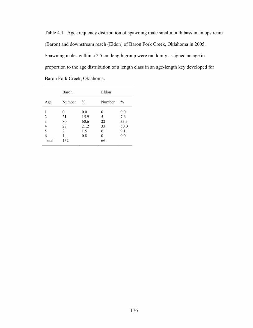
Table 4.1. Age-frequency distribution of spawning male smallmouth bass in an upstream

(Baron) and downstream reach (Eldon) of Baron Fork Creek, Oklahoma in 2005.

Spawning males within a 2.5 cm length group were randomly assigned an age in

proportion to the age distribution of a length class in an age-length key developed for

Baron Fork Creek, Oklahoma.

Baron Eldon

Age Number % Number %

1 0 0.0 0 0.0 2 21 15.9 5 7.6 3 80 60.6 22 33.3 4 28 21.2 33 50.0 5 2 1.5 6 9.1 6 1 0.8 0 0.0 Total 132 66

176

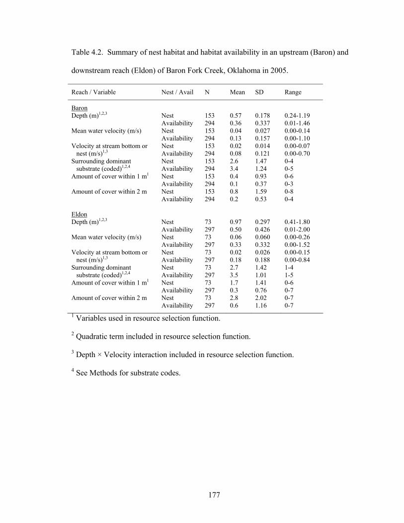
Table 4.2. Summary of nest habitat and habitat availability in an upstream (Baron) and

downstream reach (Eldon) of Baron Fork Creek, Oklahoma in 2005.

Reach / Variable Nest / Avail N Mean SD Range

Baron Depth (m)1,2,3 Nest 153 0.57 0.178 0.24-1.19 Availability 294 0.36 0.337 0.01-1.46 Mean water velocity (m/s) Nest 153 0.04 0.027 0.00-0.14 Availability 294 0.13 0.157 0.00-1.10 Velocity at stream bottom or Nest 153 0.02 0.014 0.00-0.07 nest (m/s)1,3 Availability 294 0.08 0.121 0.00-0.70 Surrounding dominant Nest 153 2.6 1.47 0-4 substrate (coded)1,2,4 Availability 294 3.4 1.24 0-5 Amount of cover within 1 m1 Nest 153 0.4 0.93 0-6 Availability 294 0.1 0.37 0-3 Amount of cover within 2 m Nest 153 0.8 1.59 0-8 Availability 294 0.2 0.53 0-4 Eldon Depth (m)1,2,3 Nest 73 0.97 0.297 0.41-1.80 Availability 297 0.50 0.426 0.01-2.00 Mean water velocity (m/s) Nest 73 0.06 0.060 0.00-0.26 Availability 297 0.33 0.332 0.00-1.52 Velocity at stream bottom or Nest 73 0.02 0.026 0.00-0.15 nest (m/s)1,3 Availability 297 0.18 0.188 0.00-0.84 Surrounding dominant Nest 73 2.7 1.42 1-4 substrate (coded)1,2,4 Availability 297 3.5 1.01 1-5 Amount of cover within 1 m1 Nest 73 1.7 1.41 0-6 Availability 297 0.3 0.76 0-7 Amount of cover within 2 m Nest 73 2.8 2.02 0-7 Availability 297 0.6 1.16 0-7 1 Variables used in resource selection function.

2 Quadratic term included in resource selection function.

3 Depth × Velocity interaction included in resource selection function.

4 See Methods for substrate codes.

177

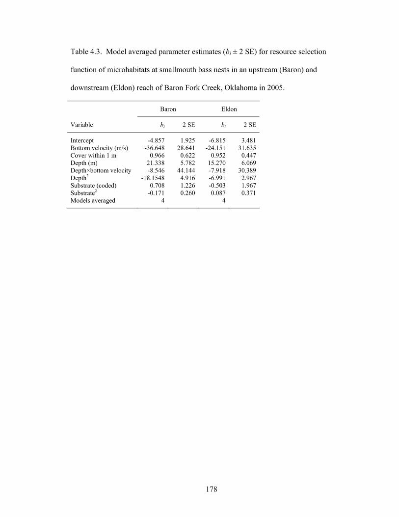
Table 4.3. Model averaged parameter estimates (bi ± 2 SE) for resource selection

function of microhabitats at smallmouth bass nests in an upstream (Baron) and

downstream (Eldon) reach of Baron Fork Creek, Oklahoma in 2005.

Baron Eldon

Variable bi 2 SE bi 2 SE

Intercept -4.857 1.925 -6.815 3.481 Bottom velocity (m/s) -36.648 28.641 -24.151 31.635 Cover within 1 m 0.966 0.622 0.952 0.447 Depth (m) 21.338 5.782 15.270 6.069 Depth×bottom velocity -8.546 44.144 -7.918 30.389 Depth2 -18.1548 4.916 -6.991 2.967 Substrate (coded) 0.708 1.226 -0.503 1.967 Substrate2 -0.171 0.260 0.087 0.371 Models averaged 4 4

178

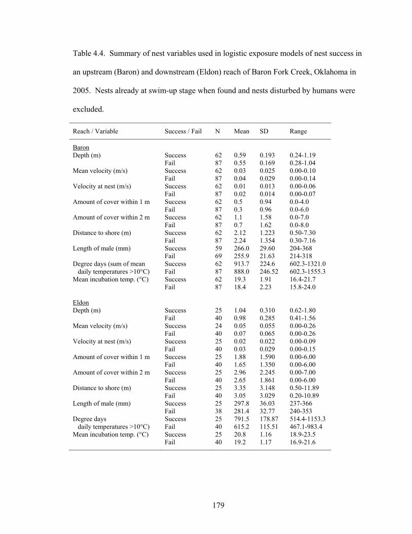
Table 4.4. Summary of nest variables used in logistic exposure models of nest success in

an upstream (Baron) and downstream (Eldon) reach of Baron Fork Creek, Oklahoma in

2005. Nests already at swim-up stage when found and nests disturbed by humans were

excluded.

Reach / Variable Success / Fail N Mean SD Range

Baron Depth (m) Success 62 0.59 0.193 0.24-1.19 Fail 87 0.55 0.169 0.28-1.04 Mean velocity (m/s) Success 62 0.03 0.025 0.00-0.10 Fail 87 0.04 0.029 0.00-0.14 Velocity at nest (m/s) Success 62 0.01 0.013 0.00-0.06 Fail 87 0.02 0.014 0.00-0.07 Amount of cover within 1 m Success 62 0.5 0.94 0.0-4.0 Fail 87 0.3 0.96 0.0-6.0 Amount of cover within 2 m Success 62 1.1 1.58 0.0-7.0 Fail 87 0.7 1.62 0.0-8.0 Distance to shore (m) Success 62 2.12 1.223 0.50-7.30 Fail 87 2.24 1.354 0.30-7.16 Length of male (mm) Success 59 266.0 29.60 204-368 Fail 69 255.9 21.63 214-318 Degree days (sum of mean Success 62 913.7 224.6 602.3-1321.0 daily temperatures >10°C) Fail 87 888.0 246.52 602.3-1555.3 Mean incubation temp. (°C) Success 62 19.3 1.91 16.4-21.7 Fail 87 18.4 2.23 15.8-24.0 Eldon Depth (m) Success 25 1.04 0.310 0.62-1.80 Fail 40 0.98 0.285 0.41-1.56 Mean velocity (m/s) Success 24 0.05 0.055 0.00-0.26 Fail 40 0.07 0.065 0.00-0.26 Velocity at nest (m/s) Success 25 0.02 0.022 0.00-0.09 Fail 40 0.03 0.029 0.00-0.15 Amount of cover within 1 m Success 25 1.88 1.590 0.00-6.00 Fail 40 1.65 1.350 0.00-6.00 Amount of cover within 2 m Success 25 2.96 2.245 0.00-7.00 Fail 40 2.65 1.861 0.00-6.00 Distance to shore (m) Success 25 3.35 3.148 0.50-11.89 Fail 40 3.05 3.029 0.20-10.89 Length of male (mm) Success 25 297.8 36.03 237-366 Fail 38 281.4 32.77 240-353 Degree days Success 25 791.5 178.87 514.4-1153.3 daily temperatures >10°C) Fail 40 615.2 115.51 467.1-983.4 Mean incubation temp. (°C) Success 25 20.8 1.16 18.9-23.5 Fail 40 19.2 1.17 16.9-21.6

179

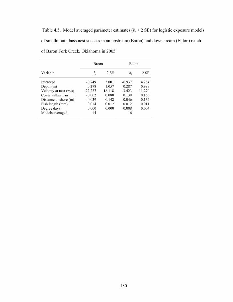
Table 4.5. Model averaged parameter estimates (bi ± 2 SE) for logistic exposure models

of smallmouth bass nest success in an upstream (Baron) and downstream (Eldon) reach

of Baron Fork Creek, Oklahoma in 2005.

Baron Eldon

Variable bi 2 SE bi 2 SE

Intercept -0.749 3.001 -6.937 4.284 Depth (m) 0.278 1.057 0.287 0.999 Velocity at nest (m/s) -22.227 18.118 -3.423 11.270 Cover within 1 m -0.002 0.080 0.138 0.165 Distance to shore (m) -0.039 0.142 0.046 0.134 Fish length (mm) 0.014 0.012 0.012 0.011 Degree days 0.000 0.000 0.008 0.004 Models averaged 14 16

180

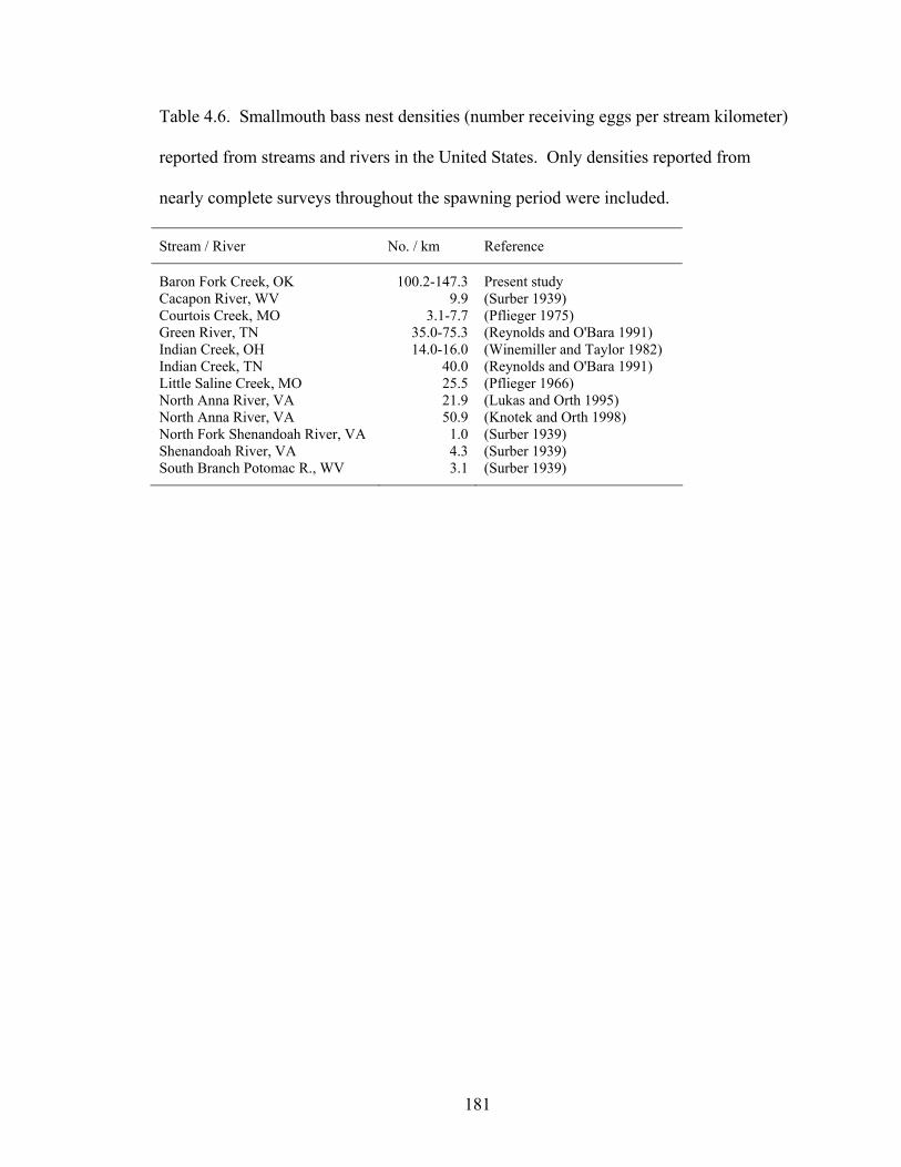
Table 4.6. Smallmouth bass nest densities (number receiving eggs per stream kilometer)

reported from streams and rivers in the United States. Only densities reported from

nearly complete surveys throughout the spawning period were included.

Stream / River No. / km Reference

Baron Fork Creek, OK 100.2-147.3 Present study Cacapon River, WV 9.9 (Surber 1939) Courtois Creek, MO 3.1-7.7 (Pflieger 1975) Green River, TN 35.0-75.3 (Reynolds and O'Bara 1991) Indian Creek, OH 14.0-16.0 (Winemiller and Taylor 1982) Indian Creek, TN 40.0 (Reynolds and O'Bara 1991) Little Saline Creek, MO 25.5 (Pflieger 1966) North Anna River, VA 21.9 (Lukas and Orth 1995) North Anna River, VA 50.9 (Knotek and Orth 1998) North Fork Shenandoah River, VA 1.0 (Surber 1939) Shenandoah River, VA 4.3 (Surber 1939) South Branch Potomac R., WV 3.1 (Surber 1939)

181

Figure 4.1. Locations of upstream (Baron) and downstream (Eldon) reaches of Baron

Fork Creek, Oklahoma whereby nesting behavior, nest site selection, and nest success of

smallmouth bass were evaluated in 2005.

Figure 4.2. Number of active smallmouth bass nests observed during snorkeling surveys

in relation to mean daily temperature and discharge in an upstream (Baron, A) and

downstream (Eldon, B) reach of Baron Fork Creek, Oklahoma in 2005. Asterisk

indicates nests receiving eggs prior to first snorkeling survey (10 May) and determined

from back-calculated dates of nest development.

Figure 4.3. Channel units and nest locations in an upstream (Baron) reach of Baron Fork

Creek, Oklahoma in 2005. 10 nests locations are missing because of errors in GPS data.

Figure 4.4. Channel units and nest locations in a downstream (Eldon) reach of Baron

Fork Creek, Oklahoma in 2005.

Figure 4.5. Number of submerged cover types (within 1 m) used by individual nesting

male smallmouth bass, and total amount of cover used by all nesting males for an

upstream (Baron, A) and downstream (Eldon, B) reach in Baron Fork Creek, Oklahoma

in 2005.

Figure 4.6. Model averaged relative probabilities of use for water depths at different

water velocities at upstream (Baron, A) and downstream (Eldon, B) reaches in Baron

182

Fork Creek, Oklahoma in 2005, and relative probabilities of use for cover at both reaches

(C). All variables were held at their mean values except the variable(s) of interest.

Figure 4.7. Conceptual model of percent of physically (solid line) or biologically (hashed

line) related nest failures during harsh versus benign streamflow conditions. Current

understanding is lacking regarding the form of physical (streamflows) versus biological

(predation) factors at intermediate streamflows, and whether they are additive or

compensatory.

183

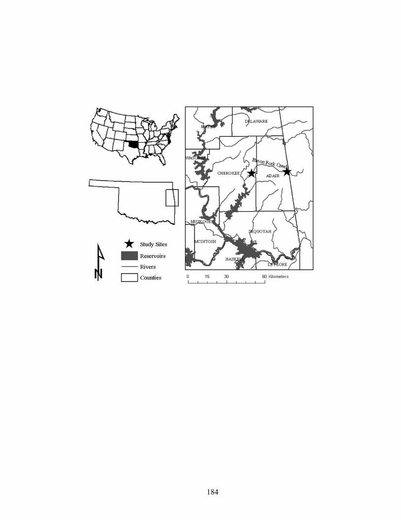
184

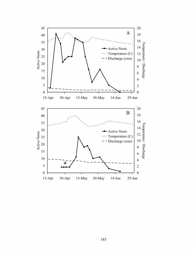
A

0

5

10

15

20

25

30

35

40

45

15-Apr 30-Apr 15-May 30-May 14-Jun 29-Jun

Act

i

0

2

4

6

8

10

12

14

16

18

20

Temperature / D

ischarge

tsve

Nes

Active NestsTemperature (C)Discharge (cms)

B

*0

5

10

15

20

25

30

35

40

45

15-Apr 30-Apr 15-May 30-May 14-Jun 29-Jun

ti

0

2

4

6

8

10

12

14

16

18

20

Temperature / D

ischarge

Active NestsTemperature (C)Discharge (cms)

tsve

Nes

Ac

185

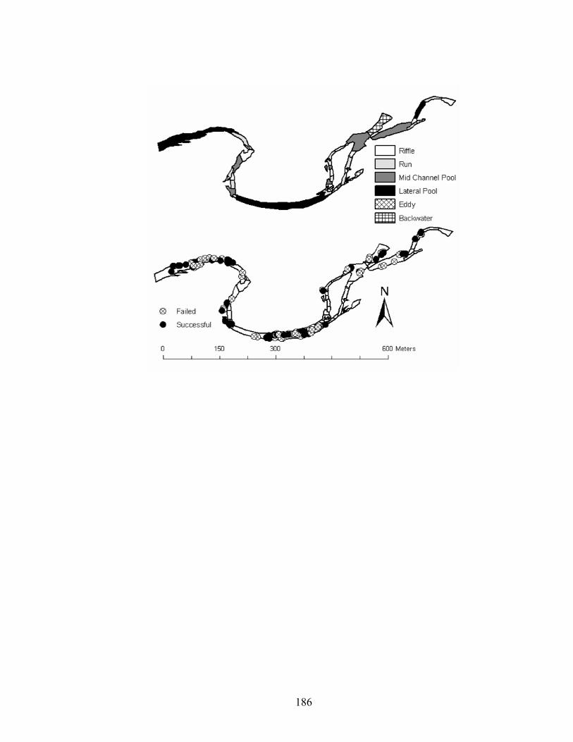
186

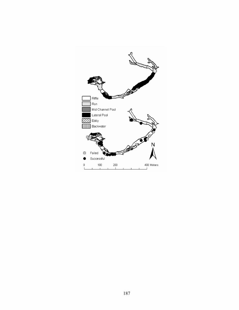
187

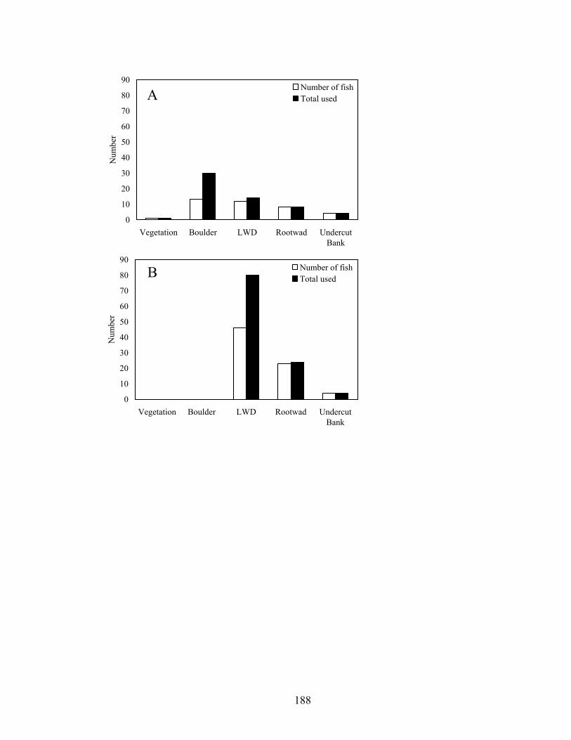
0

10

20

30

40

50

60

70

80

90

Vegetation Boulder LWD Rootwad UndercutBank

Number of fishTotal used

0

10

20

30

40

50

60

70

80

90

Vegetation Boulder LWD Rootwad UndercutBank

Num

ber

Number of fishTotal usedA

B

Num

ber

188

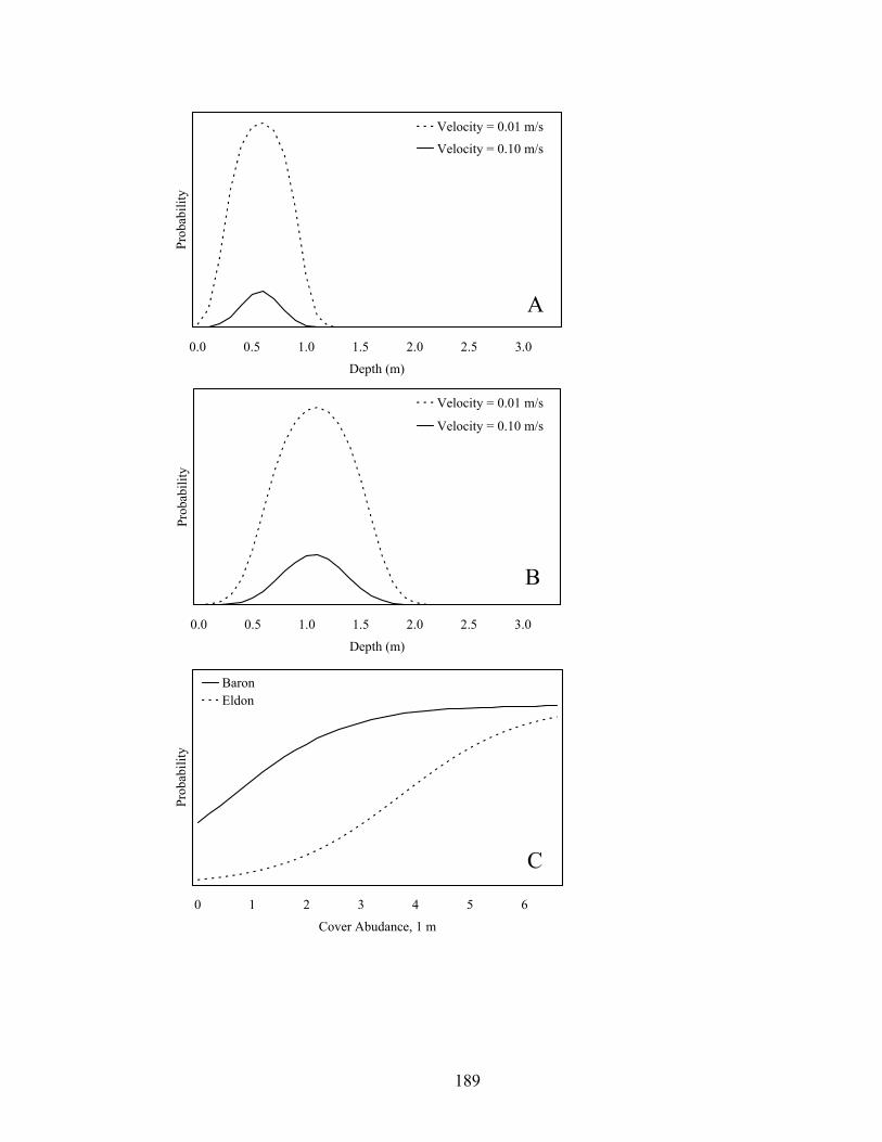
A

B

C

0.0 0.5 1.0 1.5 2.0 2.5 3.0

Depth (m)

Prob

abili

ty

Velocity = 0.01 m/s

Velocity = 0.10 m/s

0.0 0.5 1.0 1.5 2.0 2.5 3.0

Depth (m)

Prob

abili

ty

Velocity = 0.01 m/s

Velocity = 0.10 m/s

0 1 2 3 4 5 6

Cover Abudance, 1 m

Prob

abili

ty

BaronEldon

189

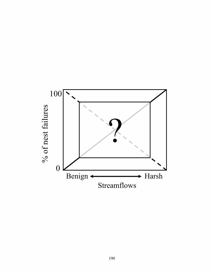
0

10

?

% o

f nes

t fai

lure

s

0

Benign Harsh

Streamflows

190

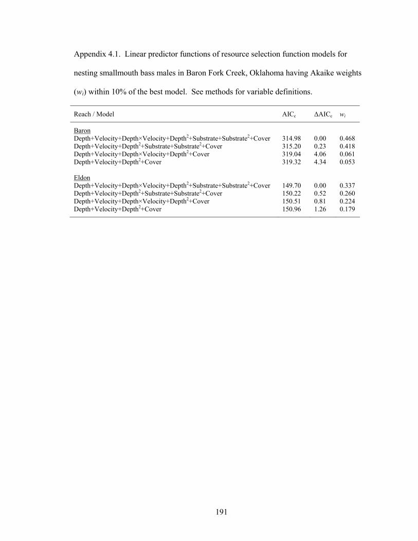
Appendix 4.1. Linear predictor functions of resource selection function models for

nesting smallmouth bass males in Baron Fork Creek, Oklahoma having Akaike weights

(wi) within 10% of the best model. See methods for variable definitions.

Reach / Model AICc ∆AICc wi

Baron Depth+Velocity+Depth×Velocity+Depth2+Substrate+Substrate2+Cover 314.98 0.00 0.468 Depth+Velocity+Depth2+Substrate+Substrate2+Cover 315.20 0.23 0.418 Depth+Velocity+Depth×Velocity+Depth2+Cover 319.04 4.06 0.061 Depth+Velocity+Depth2+Cover 319.32 4.34 0.053 Eldon Depth+Velocity+Depth×Velocity+Depth2+Substrate+Substrate2+Cover 149.70 0.00 0.337 Depth+Velocity+Depth2+Substrate+Substrate2+Cover 150.22 0.52 0.260 Depth+Velocity+Depth×Velocity+Depth2+Cover 150.51 0.81 0.224 Depth+Velocity+Depth2+Cover 150.96 1.26 0.179

191

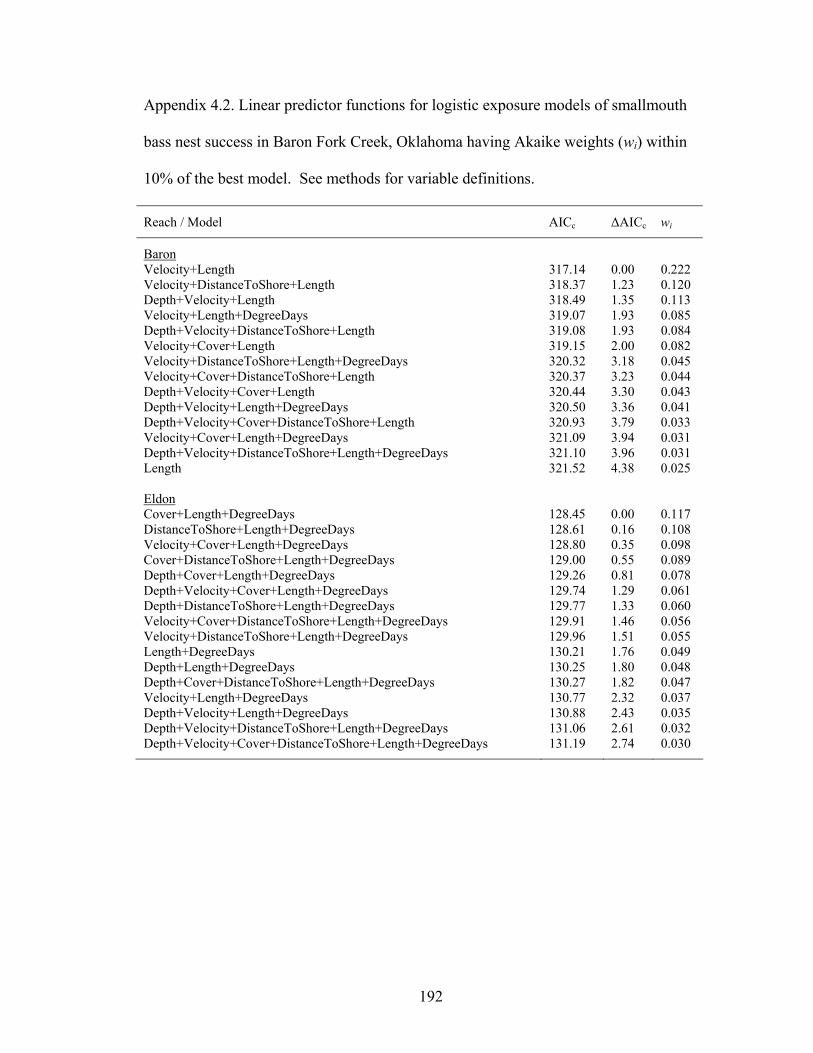
Appendix 4.2. Linear predictor functions for logistic exposure models of smallmouth

bass nest success in Baron Fork Creek, Oklahoma having Akaike weights (wi) within

10% of the best model. See methods for variable definitions.

Reach / Model AICc ∆AICc wi

Baron Velocity+Length 317.14 0.00 0.222 Velocity+DistanceToShore+Length 318.37 1.23 0.120 Depth+Velocity+Length 318.49 1.35 0.113 Velocity+Length+DegreeDays 319.07 1.93 0.085 Depth+Velocity+DistanceToShore+Length 319.08 1.93 0.084 Velocity+Cover+Length 319.15 2.00 0.082 Velocity+DistanceToShore+Length+DegreeDays 320.32 3.18 0.045 Velocity+Cover+DistanceToShore+Length 320.37 3.23 0.044 Depth+Velocity+Cover+Length 320.44 3.30 0.043 Depth+Velocity+Length+DegreeDays 320.50 3.36 0.041 Depth+Velocity+Cover+DistanceToShore+Length 320.93 3.79 0.033 Velocity+Cover+Length+DegreeDays 321.09 3.94 0.031 Depth+Velocity+DistanceToShore+Length+DegreeDays 321.10 3.96 0.031 Length 321.52 4.38 0.025 Eldon Cover+Length+DegreeDays 128.45 0.00 0.117 DistanceToShore+Length+DegreeDays 128.61 0.16 0.108 Velocity+Cover+Length+DegreeDays 128.80 0.35 0.098 Cover+DistanceToShore+Length+DegreeDays 129.00 0.55 0.089 Depth+Cover+Length+DegreeDays 129.26 0.81 0.078 Depth+Velocity+Cover+Length+DegreeDays 129.74 1.29 0.061 Depth+DistanceToShore+Length+DegreeDays 129.77 1.33 0.060 Velocity+Cover+DistanceToShore+Length+DegreeDays 129.91 1.46 0.056 Velocity+DistanceToShore+Length+DegreeDays 129.96 1.51 0.055 Length+DegreeDays 130.21 1.76 0.049 Depth+Length+DegreeDays 130.25 1.80 0.048 Depth+Cover+DistanceToShore+Length+DegreeDays 130.27 1.82 0.047 Velocity+Length+DegreeDays 130.77 2.32 0.037 Depth+Velocity+Length+DegreeDays 130.88 2.43 0.035 Depth+Velocity+DistanceToShore+Length+DegreeDays 131.06 2.61 0.032 Depth+Velocity+Cover+DistanceToShore+Length+DegreeDays 131.19 2.74 0.030

192

CHAPTER 5

RELATIONSHIPS AMONG GEOMORPHOLOGY, HABITAT, AND FISHES IN

EASTERN OKLAHOMA STREAMS: THEIR IMPORTANCE TO STREAM

RESTORATION

193

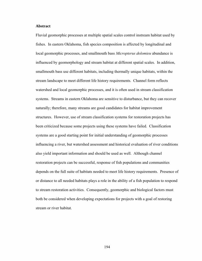
Abstract

Fluvial geomorphic processes at multiple spatial scales control instream habitat used by

fishes. In eastern Oklahoma, fish species composition is affected by longitudinal and

local geomorphic processes, and smallmouth bass Micropterus dolomieu abundance is

influenced by geomorphology and stream habitat at different spatial scales. In addition,

smallmouth bass use different habitats, including thermally unique habitats, within the

stream landscape to meet different life history requirements. Channel form reflects

watershed and local geomorphic processes, and it is often used in stream classification

systems. Streams in eastern Oklahoma are sensitive to disturbance, but they can recover

naturally; therefore, many streams are good candidates for habitat improvement

structures. However, use of stream classification systems for restoration projects has

been criticized because some projects using these systems have failed. Classification

systems are a good starting point for initial understanding of geomorphic processes

influencing a river, but watershed assessment and historical evaluation of river conditions

also yield important information and should be used as well. Although channel

restoration projects can be successful, response of fish populations and communities

depends on the full suite of habitats needed to meet life history requirements. Presence of

or distance to all needed habitats plays a role in the ability of a fish population to respond

to stream restoration activities. Consequently, geomorphic and biological factors must

both be considered when developing expectations for projects with a goal of restoring

stream or river habitat.

194

Introduction

Rivers route water and sediment downstream, and the routing processes are distributed

throughout a hierarchy of nested spatial and temporal scales (Frissell et al. 1986). At

large spatial scales, regional variation in geology, topography, climate, and land use

affect hydrologic and sediment regimes. Zones of erosion, transport, and deposition are

associated with the longitudinal profiles of streams (Knighton 1998), and water and

sediment movement through a stream reach interact with channel and bank materials

(including vegetation) to determine channel form (Leopold et al. 1964). Streamflow and

sediment regimes and channel form play a large role in riffle/pool development and

structure within a reach. The degree of spatial variability in natural (e.g., debris flows,

bedrock controls) and anthropogenic (e.g., land use) disturbances within a watershed

determine whether changes in channel form occur gradually or abruptly from upstream to

downstream (Montgomery 1999); however, some change in sediment, streamflow, or

water chemistry is expected at tributary junctions (Poole 2002; Benda et al. 2004). These

geomorphic processes are complex and interacting, and result in channel features used as

habitat by fishes at different spatial scales (Frissell et al. 1986; Rabeni and Jacobson

1993b; Walters et al. 2003).

Eastern Oklahoma streams

Channel morphology

Channel form is often used as a proxy for trends in channel process and response

(Simon and Castro 2003). As a result, channel form has been incorporated into a variety

195

of stream classifications systems, some of which are used in stream channel restoration

projects (Arend 1999; Kondolf et al. 2003). Arguably the most widely applied stream

classification system was developed by Rosgen (1994; 1996).

A survey of 155 streams, including those that were intermittent, in the Boston

Mountains, Ouachita Mountains, and Ozark Highlands (Omernik 1987) in eastern

Oklahoma revealed three Rosgen stream types, with additional subclasses (Table 5.1).

Smaller streams were more confined by valley slopes and dominated by riffles, and they

had moderate gradients and stable channel form (Rosgen Type B). However, most

streams were typically low gradient, meandering, riffle/pool, alluvial streams (Type C).

Gravel bed streams predominated, but there was more variability in sizes of surficial

substrates in the southeastern Ouachita Mountain streams (C3 [cobble] and C4 [gravel])

when compared to northeastern streams (largely C4). Some streams were low gradient,

meandering, with riffle/pool structure and stable channel form (Type E).

Geomorphology, stream habitat, and fishes

Several factors determine the fish species residing in a stream reach (Poff 1997).

Historical biogeography is important in explaining the distribution of some stream fishes

in upland regions in eastern Oklahoma (Chapter 1; Howell 2001). However, fluvial

geomorphic processes were also found to be important determinants of species

composition, among those evaluated, in eastern Oklahoma streams (Chapter 1).

Concomitant changes in physical, chemical, and biological processes with increasing

stream size were important in dictating habitat conditions and the fish species within the

regional species pool that were observed within a stream reach. However, spatial

196

variability in sediment regimes and channel cross-section form was also important in

determining fish species composition.

Smallmouth bass Micropterus dolomieu populations are largely influenced by

longitudinal processes in eastern Oklahoma streams, in addition to other factors (Chapters

2 and 3). In headwater streams, smallmouth bass populations are recruitment limited due

to streamflow dynamics and spawning habitat limitations and, therefore, are largely

absent. They are also limited in downstream reaches, likely in response to increased

water temperatures, turbidity, and fine substrates (Rabeni and Jacobson 1993a; Sowa and

Rabeni 1995). Longitudinal changes in population dynamics, however, differ between

northeastern and southeastern Oklahoma streams. In reaches with large numbers of

individuals, densities were higher in deepwater habitats. Channel morphology is also

related to smallmouth bass populations beyond the effects of stream and habitat size;

abundances are higher in larger streams with less pool area, higher channel width:depth

ratios, and gravel substrates. Habitat within channel units (vegetation, wood, bedrock)

was also related to abundance, but relations were dependent on stream size and channel

morphology.

Smallmouth bass also used different habitats within the stream landscape to meet

different life cycle requirements (Chapters 3 and 4). Food and cover availability did not

strongly influence the distribution of individuals within a reach, perhaps because they

were abundant and not limiting resources. Different complementary habitats, however,

were used for spawning and winter refugia. Smallmouth bass that remained in a reach of

Baron Fork Creek in winter moved into a backwater and adjacent habitats that had

observable groundwater influx resulting in warmer water temperatures during cold winter

197

days. These thermal characteristics were unique in summer as well, but apparently were

not important enough to be used by smallmouth bass in summer. High levels of water

exchange and mixing between subsurface flow, surface flow, and groundwater apparently

kept water temperatures low enough in the main channel during summer so thermal

refugia were not needed. In contrast, the backwater used in winter was largely unsuitable

for spawning in spring due to a thick layer of sand-silt substrates, although a few nests

were observed along the margins where some gravel was present (Chapter 4).

Use of the stream landscape by smallmouth bass was only documented in Baron

Fork Creek in northeastern Oklahoma, and it is unknown to what degree different habitats

are used by smallmouth bass in southeastern Ouachita Mountain streams. Given that

Ouachita Mountains streams are more runoff dominated and have higher water

temperatures in summer than northeastern streams (Chapter 3), summer refugia may be

important to smallmouth bass populations because of the detrimental effects that water

temperatures greater than 22°C have on the growth scope of smallmouth bass (Zweifel et

al. 1999; Whitledge et al. 2002). Interestingly, Big Eagle Creek near Octavia, LeFlore

County, Oklahoma, had consistently high channel-unit densities of smallmouth bass

during stream surveys in the Ouachita Mountains; it had the 4th through 10th highest

densities of smallmouth bass (greater than 100 mm) of all channel units sampled in the

Ouachita Mountains. It was also the only southeastern stream where a smallmouth bass

nest and individuals over 300 mm were observed while snorkeling. Big Eagle Creek was

the only stream sampled in the southeast that had a large cold-water spring adjacent to a

bedrock outcrop. Channel units with high densities of smallmouth bass were located

above and below the spring. Thus, if the spring mitigated high summer water

198

temperatures (water temperature was not measured), enhanced smallmouth bass

production and survival in this area resulted in individuals dispersing to other areas

within the reach. A better understanding is needed regarding potential summer and

winter thermal refugia in southeastern Oklahoma streams.

Stream channel and habitat restoration

Streams in eastern Oklahoma, particularly in the northeast, are sensitive to disturbances

but have a natural ability to recover. According to Rosgen’s classification system (1994;

Table 3), most stream reaches we sampled in eastern Oklahoma are sensitive to increased

streamflow magnitude and sediment loads. However, Rosgen also suggests that they

have a ‘good’ recovery potential given that factors causing stream instability are

resolved. Moreover, several instream structures suggested to improve fish habitat are

applicable to streams in eastern Oklahoma (Table 5.2). Following channel recovery, fish

species composition might also respond, because the presence or absence of fish species

is affected by channel form and sediment regimes in addition to longitudinal processes.

However, smallmouth bass were only found in large type C streams, but show substantial

variation within this stream type (Figure 5.1).

Although most stream types observed in eastern Oklahoma are good candidates

for stream habitat improvement structures, caution must be exercised when using

guidelines presented by classification schemes for such structures. Instream restoration

projects will not be successful without fully considering geomorphic processes during

restoration planning (Frissell and Nawa 1992; Kondolf et al. 2001); however, some

successful instream structures have been reported even when watershed disturbances

199

were not resolved (House 1996). Some researchers have questioned stream classification

systems designed for stream restoration and habitat improvement because they are not

linked to current channel equilibrium conditions, do not always consider larger scale

processes such as climate and hydrology, and facilitate a shortcut from a true

geomorphologic analysis of a river system (Miller and Ritter 1996; Doyle et al. 1999).

Stream classifications may be a starting point for stream restoration planning, but other

information is needed. A tiered or hierarchical approach that evaluates different spatial

and temporal scales is most informative, including watershed assessments and sediment

budgets (Kondolf 2000; Roni et al. 2002) and review of historical information (Rosgen

1996; Kondolf et al. 2003). Although a true geomorphologic analysis should include a

study of river system history to understand its past behavior, classification schemes that

describe the existing channel form, which reflects historical processes to some degree,

can facilitate communication among managers (Simon and Castro 2003; Kondolf et al.

2003). Kondolf et al. (2003) provided three reasons why classification of stream

channels is useful for stream restoration: to survey existing conditions and set restoration

priorities, to envision the end state resulting from restoration activities, and to offer

insight into restoration measures likely to be successful.

Although channel restoration or fish habitat improvement structures may be

successful from a geomorphic standpoint, additional factors dictate whether stream fishes

will respond to activity1. For example, smallmouth bass were found only in certain

Rosgen stream types, but densities varied widely within those types. So even if channel

form is restored, smallmouth bass abundances may not respond predictably because of

other important factors (stream size, habitat size, wood, vegetation; Chapter 2). In 1 Biological response may not be a priority goal of a channel restoration project.

200

addition, if a functional habitat unit, defined as the suite of habitats needed by a fish to

complete its life cycle, is incomplete, a population might not respond to the channel or

habitat modification. Moreover, the distance between required habitats will determine

the degree of response, because distance to complementary habitats affects population

dynamics and size (Schlosser 1995; Kocik and Ferreri 1998). Proximity of restoration

projects to habitats (e.g., bluff pools, backwaters, and springs) offering a thermal refuge

during winter or summer may partially dictate the type and magnitude of response by

smallmouth bass populations to instream habitat projects. Bluff pools are important

habitats for smallmouth bass, and valley walls that form bluff pools occur less often in

downstream reaches of Ozark streams (Rabeni and Jacobson 1993a). The spatial location

and frequency of bluff pools within the profile of a river may not always be predictable,

however, as happenstance contact of a river with valley walls depends on sinuosity,

channel migration rates, and the underlying structure (stratigraphy, folds, faults) of basin

lithology and valley walls themselves.

Current stream restoration principles emphasize system ecology and benefits for

stakeholders. Palmer et al. (2005) proposed five measures of restoration success: 1)

restoration project design should be based on a healthy dynamic system that can exist at a

site; 2) river ecology (including hyrdogeomorphology) should be improved; 3) the river

system must be self-sustaining and resilient to future disturbances; 4) restoration

construction should have no lasting, harmful impacts; and 5) pre- and post-project

assessment must be completed and data and results made publicly available. Many recent

projects have focused on restoring aesthetics and ecology of streams (Moerke and

Lamberti 2004), although monitoring of restoration projects has not been frequent (Roni

201

et al. 2002). However, monitoring methods (Roni 2005) are more likely to be

implemented when restoring river ecology (versus engineering) is the goal (Bash and

Ryan 2002). Project success is often difficult to ensure, however, because stream

restoration projects are poorly controlled experimentally, there is little transferability of

results from previous projects, and the projects are socially complicated and costly

(Shields et al. 2003). Furthermore, reinstating the dynamic equilibrium of rivers often

poses a safety risk for project managers who subsequently resort to use of hard

engineering (Gillilan et al. 2005). Some of these problems will likely be more difficult to

resolve with current practices focusing on larger spatial scales such as watersheds

(Williams et al. 1997; Hillman and Brierley 2005).

Conclusions

Streams reflect a multitude of terrestrial and fluvial processes intertwined in a hierarchy

of spatial and temporal scales (Frissell et al. 1986). Although study and classification of

stream reaches may yield an initial indication of river processes, a full geomorphic

analysis of several spatial scales and river history will result in the most complete

understanding of factors dictating the success of a restoration project. The suite of

habitats used by fishes or other aquatic organisms must also be considered when projects

are expected to elicit a biological response. Project success and accountability are

important because resources from public entities and private organizations are often used

for such activities (Moerke and Lamberti 2004). Failed projects waste monetary

resources. This may cause negative perceptions towards the resource agency and future

projects (Turner 1997), resulting in fewer resources allocated for future projects.

202

Therefore, consideration of a full suite of geomorphic and biological factors is crucial to

better ensure the success of any stream and river restoration program.

Acknowledgments

Project funding was provided by a Federal Aid in Sport Fish Restoration Act grant under

Project F-55-R of the Oklahoma Department of Wildlife Conservation and the Oklahoma

Cooperative Fish and Wildlife Research Unit. The Oklahoma Cooperative Fish and

Wildlife Research Unit is jointly sponsored by the U. S. Geological Survey; Oklahoma

State University; the Oklahoma Department of Wildlife Conservation; the Wildlife

Management Institute; and the U. S. Fish and Wildlife Service. D. Dauwalter was

supported by a Fellowship for Water, Energy, & the Environment from the

Environmental Institute, Oklahoma State University

References

Arend, K. K. 1999. Classification of stream reaches. Pages 57-74 in M. B. Bain and N.

J. Stevenson, editors. Aquatic habitat assessment: common methods. American

Fisheries Society, Bethesda, Maryland.

Bash, J. S. and C. M. Ryan. 2002. Stream restoration and enhancement projects: Is

anyone monitoring? Environmental Management 29:877-885.

Benda, L., N. L. Poff, D. Miller, T. Dunne, G. Reeves, G. Pess, and M. Pollock. 2004.

The network dynamics hypothesis: how channel networks structure riverine

habitat. BioScience 54:413-427.

203

Doyle, M. W., D. E. Miller, and J. M. Harbor. 1999. Should river restoration be based

on classification schemes or process models? Insights from the history of

geomorphology. ASCE International Conference on Water Resources

Engineering, Seattle, Washington.

Frissell, C. A., W. J. Liss, C. E. Warren, and M. D. Hurley. 1986. A hierarchical

framework for stream habitat classification: viewing streams in a watershed

context. Environmental Management 10:199-214.

Frissell, C. A. and R. K. Nawa. 1992. Incidence and causes of physical failure of

artificial habitat structures in streams of western Oregon and Washington. North

American Journal of Fisheries Management 12:182-197.

Gillilan, S., K. Boyd, T. Hoitsma, and M. Kauffman. 2005. Challenges in developing

and implementing ecological standards for geomorphic river restoration projects:

a practitioner's response to Palmer et al. (2005). Journal of Applied Ecology

42:223-227.

Hillman, M. and G. Brierley. 2005. A critical review of catchment-scale stream

rehabilitation programmes. Progress in Physical Geography 29:50-76.

House, R. 1996. An evaluation of stream restoration structures in a coastal Oregon

stream 1981-1993. North American Journal of Fisheries Management 16:272-

281.

Howell, C. E. Jr. 2001. Correspondence between aquatic ecoregions and the distribution

of fish communities of eastern Oklahoma. M.S. Thesis. University of North

Texas, Denton, Texas.

204

Knighton, D. 1998. Fluvial forms and processes: a new perspective. Oxford University

Press, Inc., New York.

Kocik, J. F. and C. P. Ferreri. 1998. Juvenile production variation in salmonids:

population dynamics, habitat, and the role of spatial relationships. Canadian

Journal of Fisheries and Aquatic Sciences 55:191-200.

Kondolf, G. M., M. W. Smeltzer, and S. F. Railsback. 2001. Design and performance of

a channel reconstruction project in a coastal California gravel-bed stream.

Environmental Management 28:761-776.

Kondolf, G. M. 2000. Some suggested guidelines for geomorphic aspects of

anadromous salmonid habitat restoration. Restoration Ecology 8:48-56.

Kondolf, G. M., D. R. Montgomery, H. Piéjay, and L. Schmitt. 2003. Geomorphic

classification of rivers and streams. Pages 171-204 in G. M. Kondolf and H.

Piéjay, editors. Tools in geomorphology. John Wiley & Sons Ltd., West Sussex,

England.

Leopold, L. B., M. G. Wolman, and J. P. Miller. 1964. Fluvial processes in

geomorphology. Dover Publications, Inc., New York.

Miller, J. R. and J. B. Ritter. 1996. An examination of the Rosgen classification of

natural rivers. Catena 27:295-299.

Moerke, A. H. and G. A. Lamberti. 2004. Restoring stream ecosystems: Lessons from a

midwestern state. Restoration Ecology 12:327-334.

Montgomery, D. R. 1999. Process domains and the river continuum. Journal of the

American Water Resources Association 36:397-410.

205

Omernik, J. M. 1987. Ecoregions of the conterminous United States. Annals of the

Association of American Geographers 77:118-125.

Palmer, M. A., E. S. Bernhardt, J. D. Allan, P. S. Lake, G. Alexander, S. Brooks, J. Carr,

S. Clayton, C. N. Dahm, J. Follstad Shah, D. L. Galat, S. G. Loss, P. Goodwin, D.

D. Hart, B. Hassett, R. Jenkinson, G. M. Kondolf, R. Lave, J. L. Meyer, T. K.

O'Donnell, L. Pagano, and E. Sudduth. 2005. Standards for ecologically

successful river restoration. Journal of Applied Ecology 42:208-217.

Poff, N. L. 1997. Landscape filters and species traits: towards mechanistic

understanding and prediction in stream ecology. Journal of the North American

Benthological Society 16:391-409.

Poole, G. C. 2002. Fluvial landscape ecology: addressing uniqueness within the river

discontinuum. Freshwater Biology 47:641-660.

Rabeni, C. F. and R. B. Jacobson. 1993a. Geomorphic and hydraulic influences on the

abundance and distribution of stream centrarchids in Ozark USA streams. Polskie

Archiwum Hydrobiologii 40:87-99.

Rabeni, C. F. and R. B. Jacobson. 1993b. The importance of fluvial hydraulics to fish-

habitat restoration in low-gradient alluvial streams. Freshwater Biology 29:211-

220.

Roni, P. 2005. Monitoring stream and watershed restoration. American Fisheries

Society, Bethesda, Maryland.

Roni, P., T. J. Beechie, R. E. Bilby, F. E. Leonetti, M. M. Pollock, and G. R. Pess. 2002.

A review of stream restoration techniques and a hierarchical strategy for

206

prioritizing restoration in Pacific Northwest watersheds. North American Journal

of Fisheries Management 22:1-20.

Rosgen, D. L. 1994. A classification of natural rivers. Catena 22:169-199.

Rosgen, D. L. 1996. Applied river morphology. Wildland Hydrology, Pagosa Springs,

Colorado.

Schlosser, I. J. 1995. Critical landscape attributes that influence fish population

dynamics in head water streams. Hydrobiologia 303:71-81.

Shields, F. D., J. Cooper, S. S. Knight, and M. T. Moore. 2003. Stream corridor

restoration research: a long and winding road. Ecological Engineering 20:441-

454.

Simon, A. and J. Castro. 2003. Measurement and analysis of alluvial channel form.

Pages 291-322 in G. M. Kondolf and H. Piéjay, editors. Tools in geomorphology.

John Wiley & Sons Ltd., West Sussex, England.

Sowa, S. P. and C. F. Rabeni. 1995. Regional evaluation of the relation of habitat to

distribution and abundance of smallmouth bass and largemouth bass in Missouri

streams. Transactions of the American Fisheries Society 124:240-251.

Turner, W. M. 1997. Acheiving private-sector involvement and its implications for

resource professionals. Pages 158-176 in J. E. Williams, C. A. Wood, and M. P.

Dombeck, editors. Watershed restoration: principles and practices. American

Fisheries Society, Bethesda, Maryland.

Walters, D. M., D. S. Leigh, M. C. Freeman, B. J. Freeman, and C. M. Pringle. 2003.

Geomorphology and fish assemblages in a Piedmont river basin, U.S.A.

Freshwater Biology 48:1950-1970.

207

Whitledge, G. W., R. S. Hayward, and C. F. Rabeni. 2002. Effects of temperature on

specific daily metabolic demand and growth scope of sub-adult and adult

smallmouth bass. Journal of Freshwater Ecology 17:353-361.

Williams, J. E., C. A. Wood, and M. P. Dombeck. 1997. Watershed restoration:

principles and practices. American Fisheries Society, Bethesda, Maryland.

Zweifel, R. D., R. S. Hayward, and C. F. Rabeni. 1999. Bioenergetics insight into black

bass distribution shifts in Ozark border region streams. North American Journal

of Fisheries Management 19:192-197.

208

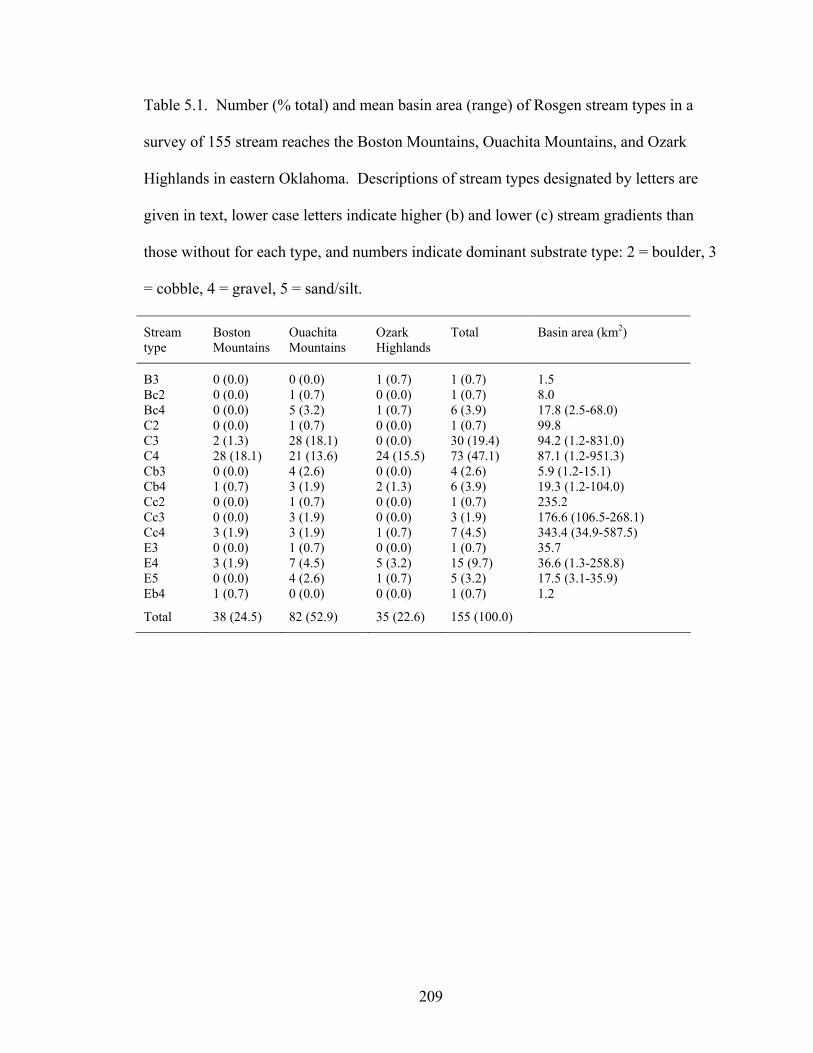
Table 5.1. Number (% total) and mean basin area (range) of Rosgen stream types in a

survey of 155 stream reaches the Boston Mountains, Ouachita Mountains, and Ozark

Highlands in eastern Oklahoma. Descriptions of stream types designated by letters are

given in text, lower case letters indicate higher (b) and lower (c) stream gradients than

those without for each type, and numbers indicate dominant substrate type: 2 = boulder, 3

= cobble, 4 = gravel, 5 = sand/silt.

Stream type

Boston Mountains

Ouachita Mountains

Ozark Highlands

Total Basin area (km2)

B3 0 (0.0) 0 (0.0) 1 (0.7) 1 (0.7) 1.5 Bc2 0 (0.0) 1 (0.7) 0 (0.0) 1 (0.7) 8.0 Bc4 0 (0.0) 5 (3.2) 1 (0.7) 6 (3.9) 17.8 (2.5-68.0) C2 0 (0.0) 1 (0.7) 0 (0.0) 1 (0.7) 99.8 C3 2 (1.3) 28 (18.1) 0 (0.0) 30 (19.4) 94.2 (1.2-831.0) C4 28 (18.1) 21 (13.6) 24 (15.5) 73 (47.1) 87.1 (1.2-951.3) Cb3 0 (0.0) 4 (2.6) 0 (0.0) 4 (2.6) 5.9 (1.2-15.1) Cb4 1 (0.7) 3 (1.9) 2 (1.3) 6 (3.9) 19.3 (1.2-104.0) Cc2 0 (0.0) 1 (0.7) 0 (0.0) 1 (0.7) 235.2 Cc3 0 (0.0) 3 (1.9) 0 (0.0) 3 (1.9) 176.6 (106.5-268.1) Cc4 3 (1.9) 3 (1.9) 1 (0.7) 7 (4.5) 343.4 (34.9-587.5) E3 0 (0.0) 1 (0.7) 0 (0.0) 1 (0.7) 35.7 E4 3 (1.9) 7 (4.5) 5 (3.2) 15 (9.7) 36.6 (1.3-258.8) E5 0 (0.0) 4 (2.6) 1 (0.7) 5 (3.2) 17.5 (3.1-35.9) Eb4 1 (0.7) 0 (0.0) 0 (0.0) 1 (0.7) 1.2

Total 38 (24.5) 82 (52.9) 35 (22.6) 155 (100.0)

209

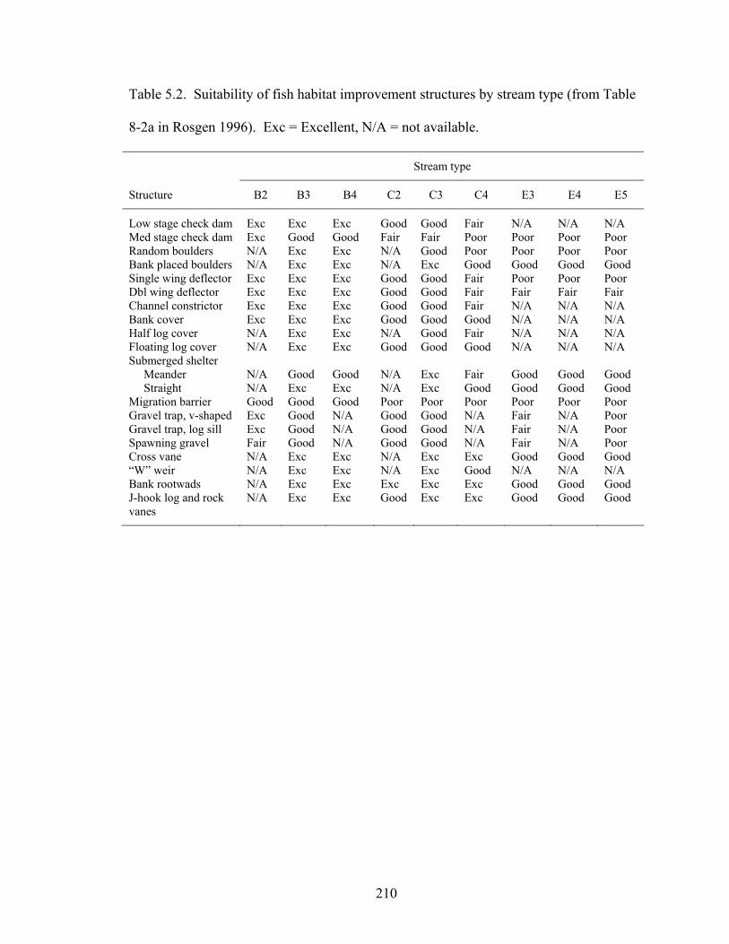
Table 5.2. Suitability of fish habitat improvement structures by stream type (from Table

8-2a in Rosgen 1996). Exc = Excellent, N/A = not available.

Stream type

Structure B2 B3 B4 C2 C3 C4 E3 E4 E5

Low stage check dam Exc Exc Exc Good Good Fair N/A N/A N/A Med stage check dam Exc Good Good Fair Fair Poor Poor Poor Poor Random boulders N/A Exc Exc N/A Good Poor Poor Poor Poor Bank placed boulders N/A Exc Exc N/A Exc Good Good Good Good Single wing deflector Exc Exc Exc Good Good Fair Poor Poor Poor Dbl wing deflector Exc Exc Exc Good Good Fair Fair Fair Fair Channel constrictor Exc Exc Exc Good Good Fair N/A N/A N/A Bank cover Exc Exc Exc Good Good Good N/A N/A N/A Half log cover N/A Exc Exc N/A Good Fair N/A N/A N/A Floating log cover N/A Exc Exc Good Good Good N/A N/A N/A Submerged shelter Meander N/A Good Good N/A Exc Fair Good Good Good Straight N/A Exc Exc N/A Exc Good Good Good Good Migration barrier Good Good Good Poor Poor Poor Poor Poor Poor Gravel trap, v-shaped Exc Good N/A Good Good N/A Fair N/A Poor Gravel trap, log sill Exc Good N/A Good Good N/A Fair N/A Poor Spawning gravel Fair Good N/A Good Good N/A Fair N/A Poor Cross vane N/A Exc Exc N/A Exc Exc Good Good Good “W” weir N/A Exc Exc N/A Exc Good N/A N/A N/A Bank rootwads N/A Exc Exc Exc Exc Exc Good Good Good J-hook log and rock vanes

N/A Exc Exc Good Exc Exc Good Good Good

210

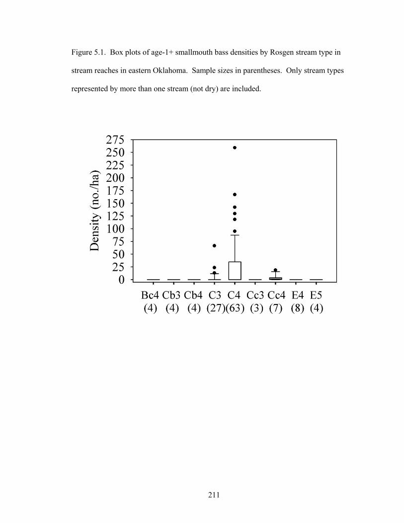
211

Figure 5.1. Box plots of age-1+ smallmouth bass densities by Rosgen stream type in

stream reaches in eastern Oklahoma. Sample sizes in parentheses. Only stream types

represented by more than one stream (not dry) are included.

VITA

Daniel Carl Dauwalter

Candidate for the Degree of

Doctor of Philosophy

Dissertation: RELATIONSHIPS AMONG GEOMORPHOLOGY, HABITAT, AND FISHES IN EASTERN OKLAHOMA STREAMS: IMPLICATIONS FOR STREAM RESTORATION

Major Field: Wildlife and Fisheries Ecology Biographical: Personal Information: Born in Carver, Minnesota, May 28th, 1977 to Mary

Sexton and Roger Dauwalter (deceased). Education: Received a Bachelor of Arts, double majoring in Biology and

Environmental Studies, from Gustavus Adolphus College in May 1999. Received a Master of Science in Aquaculture/Fisheries from University of Arkansas at Pine Bluff in May 2002. Completed requirements for the Doctor of Philosophy degree in May, 2006

Professional Experience: Employed by Carver County Environmental

Services as a Water Quality Intern from May to August, 1998. Employed by Biology Department, Gustavus Adolphus College as a Research Technician from August 1998 to May 1999. Employed by South Dakota Cooperative Fish and Wildlife Research Unit as a Fisheries Technician from May 1999 to October 1999. Employed by Department of Aquaculture and Fisheries, University of Arkansas at Pine Bluff as a Graduate Research Assistant from November 1999 to January 2002, and as a Research Associate from January 2002 to July 2002. Employed by the Oklahoma Cooperative Fish and Wildlife Research Unit as a Graduate Research Associate from July 2002 to April 2006.

Professional Memberships: Oklahoma Chapter, Southern Division, and

Parent Society of the American Fisheries Society; Oklahoma Academy of Sciences; Sigma Xi; Ecological Society of America.

Name: Daniel Carl Dauwalter Date of Degree: May, 2006 Institution: Oklahoma State University Location: Stillwater, Oklahoma Title of Study: RELATIONSHIPS AMONG GEOMORPHOLOGY, HABITAT, AND

FISHES IN EASTERN OKLAHOMA STREAMS: IMPLICATIONS FOR STREAM RESTORATION

Pages in Study: 211 Candidate for the Degree of Doctor of Philosophy Major Field: Wildlife and Fisheries Ecology Scope and Method of Study: Stream restoration is a multidisciplinary practice aimed at

reestablishing disturbed stream ecosystems. Fluvial geomorphology and landscape ecology have been individually incorporated into stream fish ecology. However, they have not been explicitly integrated into stream restoration practices. We used a stream survey to relate geomorphology and habitat to fish species composition and smallmouth bass Micropterus dolomieu abundance at several spatial scales in eastern Oklahoma streams. Spatial and temporal changes in stream habitat and population characteristics of smallmouth bass were determined for two eastern Oklahoma streams, and a landscape model was evaluated for smallmouth bass in Baron Fork Creek, Oklahoma.

Findings and Conclusions: Stream survey results elucidated complex relationships

between stream geomorphology and stream habitat, and fishes in eastern Oklahoma streams. Geomorphic variables representing stream size best explained variability in fish species composition in both northeastern and southeastern Oklahoma streams. Local channel morphology and substrate characteristics were secondarily important and mostly independent of stream size. Stream size and morphology explained variation in densities of all sizes of smallmouth bass, but channel unit habitat explained additional variation in densities of larger individuals. Stream habitat and smallmouth bass populations in Baron Fork Creek and Glover River were spatially and temporally dynamic. Water temperatures, streamflows, and instream habitat differed between streams and longitudinally within each stream. Abundance, recruitment, and survival of smallmouth bass populations differed between streams and seasons, and longitudinal patterns of these characteristics were unique in each stream. Smallmouth bass showed strong patterns of seasonal habitat complementation and supplementation: different habitats were used for spawning and summer growing periods versus those used for winter thermal refugia. Eastern Oklahoma streams are sensitive to disturbance but naturally resilient. Consideration of geomorphic relationships with fishes and ensuring that all habitats required by fishes are available will best facilitate responses from fish populations during the restoration of eastern Oklahoma streams.

Advisor’s Approval:___ _____________________________________r

______________William L. Fishe