Embed Size (px)
Citation preview

New Methods of Visualization of
Multivariable Spatio-temporal Data: PCP-
Time-Cube and Multivariable-Time-
Cube
Xia Li March, 2005

New Methods of Visualization of Multivariable Spatio-temporal Data: PCP-Time-Cube and Multivariable-Time-
Cube
by
Xia Li Thesis submitted to the International Institute for Geo-information Science and Earth Observation in partial fulfilment of the requirements for the degree in Master of Science in Geoinformatics Thesis Assessment Board Chairman: Prof. Dr. Ir. A. Stein External examiner: Prof. Dr. F.J. Ormeling Supervisor: Prof. Dr. M.J. Kraak Second supervisor: Ms Dr. C.A. Blok
INTERNATIONAL INSTITUTE FOR GEO-INFORMATION SCIENCE AND EARTH OBSERVATION ENSCHEDE, THE NETHERLANDS

Disclaimer This document describes work undertaken as part of a programme of study at the International Institute for Geo-information Science and Earth Observation. All views and opinions expressed therein remain the sole responsibility of the author, and do not necessarily represent those of the institute.

i
Abstract
Multivariable spatio-temporal data is used to describe the change of characteristics of objects with time and location, and the change in location of objects is also considered. The analysis of this kind of data is an important and challenging task, since analysts are interesting in patterns, correlations or exceptions in multivariable spatio-temporal data. They want (for example) to know not only where they are, when to arrive, but also, what the situation is, how the environment is etc. To study multivariable spatio-temporal data, data visualization is one of the effective techniques. However, currently existing methods are good at visualizing spatio-temporal data or multivariable data, not both together. Based on analysis of the multivariable spatio-temporal data and reviewing of existing visualization techniques, this paper introduces two new approaches for visualizing multivariable spatio-temporal data, called PCP-Time-Cube and Multivariable-Time-Cube. The PCP-Time-Cube is a combination of the Space-Time-Cube and existing multivariable graphics: Parallel Coordinates Plots (PCP). Based on the model design, the PCP-Time-Cube prototype is designed and realized in the ArcScene environment and SARS data is used as case study. The Multivariable-Time-Cube is designed by optional definition of the X and Y axes (Z-axis is time by default) and making a 3D view of any of the attributes in which user is interested. Similar with the PCP-Time-Cube, the Multivariable-Time-Cube prototype is designed and realized in the ArcScene environment and SARS data is used as case study. Both the PCP-Time-Cube and the Multivariable-Time-Cube are 3D visualizations of multivariable temporal data. So the Space-Time-Cube and 2D map are used to supply according geo-information. Furthermore, the usability of these two prototypes are evaluated and compared. The results of the evaluation are only preliminary ones due to the time constraint. Finally, the conclusions and recommendations in this research are discussed.
Keywords: Multivariable spatio-temporal data, Visualization methods, PCP-Time-Cube, Multivariable-Time-Cube, Usability evaluation.

ii
Acknowledgements
For the period of my study in ITC, many people helped me and made me feel at home. Here, I would like to take the opportunity to express my deepest gratitude to all the people who have provided me support and help in the study and research work. First, I would like to express my gratitude to ITC for giving me the opportunity to complete my MSc thesis. Without the help of ITC, this research could not have been completed. ITC provided me the chance to improve my scientific knowledge and enrich my personal life. I am also grateful to my department in China, ShaanXi bureau of surveying and mapping, for providing me the opportunity to study in ITC, and specifically the director Dr. Li Pengde for granting me academic leave for one and half years. I wish to express my sincere thanks and appreciation to my supervisors, Prof. Dr. Menno-Jan Kraak for his carefully thought-about advices and cautions and patience to even the smallest of the details of my work. I have learned how to conduct a scientific research and will benefit from it my whole life. Similarly, my sincere thanks go to Ms. Dr. Connie Blok, for installing evaluation into this work to ensure a successful achievement of the objectives of the study and what you have done for me move me so deep that I will never forget it.. I appreciate Ms. Y. Yuxian Sun for her patient suggestion and help in technical issues and English, without her encouragement and advise, I couldn’t pass through the difficulties in the period of my research. Similarly, my sincere thanks go to M.Sc. Gerrit Huurneman, Dr. Wangning Peng, Dr. Ir. Rolf de By and Dr. Andreas Wytzisk for their help and their critical comments and remarks to improve my research work. I would like to say that your openness, enthusiasm and encouragement will influence my whole life. All staff of the Division of GIP can never be thanked enough for their support and help. Special thanks go to my dear friends, Tina Tian, Guo Jinghua, Wu Guofeng, Wang Tiejun, Ma zhiming, Zhao Zheng and Lin Wenjing who not only helped me in the chapter reviews and content, but also encouraged me during my thesis writing. I would like to express my gratitude to all the classmates of GFM 2003, especially to Jennifer Asiedu Dartey, Xu Hixian, Wang xiankun, Jorge Ramirez, Umamaheshwaran Rajasekar, Gustavo Arciniegas, and Jorge Mario Aceituno, for their encouragement, friendship and all the pleasure that we have shared. Last but not least, my special thanks go to my beloved parents, my friends for your understanding and spiritual support. You are all in my heart.
iii
Table of contents
1. Introduction ......................................................................................................................................1
1.1. Motivation...............................................................................................................................1 1.2. Background and problem definition .......................................................................................1
1.2.1. Background.........................................................................................................................1 1.2.2. Problem definition and research objective .........................................................................2
1.3. Research questions..................................................................................................................3 1.4. Methodologies ........................................................................................................................4 1.5. Thesis structure.......................................................................................................................4
2. State-of-the-art in multivarable spatio-temporal data visualization.................................................5 2.1. Introduction.............................................................................................................................5 2.2. Multivariable spatio-temporal data.........................................................................................5
2.2.1. Spatio-temporal data...........................................................................................................5 2.2.2. Multivariable data...............................................................................................................6
2.3. Visualization solutions ...........................................................................................................8 2.3.1. Existing visualization for spatio-temporal data..................................................................8 2.3.2. Visualization for multivariable data .................................................................................18
2.4. Summary ...............................................................................................................................24 3. Models design ................................................................................................................................25
3.1. Introduction...........................................................................................................................25 3.2. Multivariable-Time-Cube .....................................................................................................25
3.2.1. Why Multivariable-Time-Cube ........................................................................................25 3.2.2. Multivariable-Time-Cube model......................................................................................26 3.2.3. Questions about multivariable spatio-temporal data in the Multivariable-Time-Cube....28 3.2.4. Design of interfaces and functions for Multivariable-Time-Cube ...................................31
3.3. PCP(parallel coordinates Plots)-time cube ...........................................................................32 3.3.1. Why PCP-Time-Cube.......................................................................................................32 3.3.2. PCP-Time-Cube model.....................................................................................................33 3.3.3. Questions about multivariable spatio-temporal data in the PCP-Time-Cube ..................34 3.3.4. “Where” in PCP-Time-Cube ............................................................................................36 3.3.5. Design of interfaces and functions for the PCP-Time-Cube ............................................38
3.4. Summary ...............................................................................................................................40 4. Prototype development and Case study .........................................................................................41
4.1. Introduction...........................................................................................................................41 4.2. The case study.......................................................................................................................41
4.2.1. Collecting data..................................................................................................................41 4.2.2. Database design ................................................................................................................42
4.3. Software and plug-in code ....................................................................................................45 4.3.1. ArcGIS..............................................................................................................................45 4.3.2. ArcGIS limitation .............................................................................................................46
4.4. Realize the PCP-Time-Cube .................................................................................................47 4.4.1. Realization of PCP-Time-Cube with SARS case .............................................................48

iv
4.4.2. Interface of prototype design............................................................................................51 4.4.3. Questions about multivariable spatio-temporal data in PCP-Time-Cube ........................53 4.4.4. Summary of PCP-Time-Cube...........................................................................................58
4.5. Realize the Multivariable-Time-Cube ..................................................................................59 4.5.1. Realization of Multivariable-Time-Cube with SARS case study.....................................59 4.5.2. Prototype interface ...........................................................................................................60 4.5.3. The questions about Multivariable spatio-temporal data in Multivariable-Time-Cube...65 4.5.4. Summary of Multivariable-Time-Cube ............................................................................67
4.6. Summary ...............................................................................................................................68 5. Usability evaluation of prototypes .................................................................................................69
5.1. Introduction...........................................................................................................................69 5.2. Evaluation objective .............................................................................................................69 5.3. Evaluation .............................................................................................................................70
5.3.1. Focus groups evaluation ...................................................................................................70 5.3.2. Questionnaire evaluation..................................................................................................70 5.3.3. Evaluation plan and overview ..........................................................................................70 5.3.4. Evaluation members .........................................................................................................71 5.3.5. Tasks design .....................................................................................................................71 5.3.6. Evaluation sessions...........................................................................................................72
5.4. Evaluation results..................................................................................................................73 5.4.1. Intelligibility and manoeuvrability ...................................................................................73 5.4.2. Efficiency .........................................................................................................................74 5.4.3. The evaluation of the geo-visitation environments ..........................................................76 5.4.4. Evaluation about addressing multivariable spatio-temporal data in two prototypes........77 5.4.5. 2D map and Space-Time-Cube.........................................................................................78
5.5. Summary ...............................................................................................................................78 6. Conclusions and further work ........................................................................................................79
6.1. Conclusions and disucssions.................................................................................................79 6.1.1. Multivariable spatio-temporal data ..................................................................................79 6.1.2. PCP-Time-Cube................................................................................................................80 6.1.3. Multivariable-Time-Cube.................................................................................................81 6.1.4. Other conclusions in this research....................................................................................83
6.2. Further work .........................................................................................................................83 Bibliography...........................................................................................................................................84 Appendix ................................................................................................................................................89

v
List of figures
Figure 1 Problem definition in this research............................................................................................3 Figure 2 Concept of spatio-temporal data after Peuquet..........................................................................5 Figure 3 Extend of Peuquet’s concept as give in figure 2........................................................................7 Figure 4 A simple representations of multivariable spatio-temporal questions based on “what”, “when”, where” and “how”......................................................................................................................7 Figure 5 Napoleon's Russian campaign of 1812 (copy for http://www.itc.nl/PERSONAL/KRAAK/) ..8 Figure 6 Sample of static map: area increase of Enschede city (copy from lecture handout of Blok, 2004) ........................................................................................................................................................9 Figure 7 Sample of series map of static: area increase of Enschede city (copy from lecture handout of Blok 2004)................................................................................................................................................9 Figure 8 Space-Time-Cube model (copy from lecture handout of Kraak (2003) in ITC) ....................11 Figure 9 Napoleon's Russian campaign in Space-Time-Cube (copy from lecture handout of Kraak 2003 in ITC) ...........................................................................................................................................11 Figure 10 Animation in Space-Time-Cube ............................................................................................13 Figure 11 Design the Function Based on question.................................................................................13 Figure 12 The corresponding relationship between Space-Time-Cube and three components concept from Peuquet (1994) ..............................................................................................................................13 Figure 13 “When+what�where” (the black line) and where+what�when (the red line) in Space-Time-Cube..............................................................................................................................................14 Figure 14 What did appear at the certain location .................................................................................15 Figure 15 What is the location of the objects at a certain time (extract a time plane in Space-Time-Cube) ......................................................................................................................................................15 Figure 16 Chernoff face in Space-Time-Cube .......................................................................................17 Figure 17 Parallel Coordinates plot .......................................................................................................19 Figure 18 Typical axis value designation hides temporal trends (left). Axis values that are consistent across time axes reveal temporal features (e.g., most observations reach their minimum temperature at 6:00 am right). ........................................................................................................................................20 Figure 19 Chernoff face graphic (Copy from the lecture handout of Kraak 2003 in ITC)....................21 Figure 20 Circle view (copy from Keim, 2003).....................................................................................21 Figure 21 Time reference in circle view (copy from Keim 2003) .........................................................22 Figure 22 Pixel bar charts ......................................................................................................................23 Figure 23 Multivariable-Time-Cube and multivariable spatio-temporal data model ............................26 Figure 24 Multivariable-Time-Cube model ...........................................................................................27 Figure 25 Projection graphic in Space-Time-Cube and Multivariable-Time-Cube...............................28 Figure 26 The steps of answering the question of where� when+ what+ how...................................29 Figure 27 The steps of answering the question of how� when+ what+ where....................................30 Figure 28 Draft interface of Multivariable-Time-Cube .........................................................................31 Figure 29 Relationship between PCP-Time-Cube and V-time plane, T-variable plane .......................34 Figure 30 T0-PCP plane is extracted from PCP-Time-Cube to answer when� what+how in PCP-Time-Cube..............................................................................................................................................35 Figure 31 “What” in PCP-Time-Cube is a surface shown in blue .........................................................36 Figure 32 V1-time plane is extracted from PCP-Time-Cube.................................................................36

vi
Figure 33 Link 2D map with PCP-Time-Cube.......................................................................................37 Figure 34 Link between Space-Time-Cube and PCP-Time-Cube ........................................................37 Figure 35 Draft interface of PCP-Time-Cube ........................................................................................39 Figure 36 Animation with synchronism reference.................................................................................40 Figure 37 Relationship diagram of the SARS database .........................................................................43 Figure 38 The 3D view tool in ArcScene (copy from ArcScene software) ..........................................46 Figure 39 Overview about Hainan province in PCP-Time-Cube...........................................................49 Figure 40 View the cube from different aspect.....................................................................................49 Figure 41 Overview of PCP-Time-Cube about three provinces ............................................................50 Figure 42 Overview of PCP-Time-Cube from top .................................................................................51 Figure 43 PCP-Time-Cube toolbars .......................................................................................................52 Figure 44 2D map view in PCP-Time-Cube ..........................................................................................52 Figure 45 An example of 2D graph view about trade-coefficient-time plane .......................................52 Figure 46 Identify result window...........................................................................................................53 Figure 47 Hainan province is characterized in PCP-Time-Cube, 2D map and identify window. .........54 Figure 48 Chongqin province is highlighted in January-PCP plane and 2D map..................................55 Figure 49 Identify provinces which near by Beijing..............................................................................56 Figure 50 Hainan province in PCP-Time-Cube and 2D map.................................................................56 Figure 51 Trade-time plane for different provinces extracted from PCP-Time-Cube...........................57 Figure 52 A province of Shandong is highlighted .................................................................................57 Figure 53 An overview of 4 provinces...................................................................................................58 Figure 54 Reference of Multivariable-Time-Cube.................................................................................60 Figure 55 Toolbar of Multivariable-Time-Cube ....................................................................................60 Figure 56 Parameters option for cubes...................................................................................................61 Figure 57 Synchronism reference definition window and identify section window .............................61 Figure 58 Patient whose id is “1” identified in Multivariable-Time-Cube............................................62 Figure 59 SARS variable change with time graphic ..............................................................................63 Figure 60 Fever state is represent as red and un-fever is represent as blue ...........................................64 Figure 61 Danger trip is represent as red line. .......................................................................................64 Figure 62 A time plane identify a time in Multivariable-Time-Cube ....................................................65 Figure 63 A patient is highlighted in Multivariable-Time-Cube and 2D graph. In 2D graph (V1-time), the patient dead because the body-temperature become 0 at 25/5/2004................................................66 Figure 64 Views from different aspect in PCP-Time-Cube...................................................................77

vii
List of tables
Table 1 Patient table...............................................................................................................................42 Table 2 PatMove table ..........................................................................................................................42 Table 3 PatSituation table ......................................................................................................................44 Table 4 ProvDaySARS table..................................................................................................................45 Table 5 Province table............................................................................................................................45 Table 6 ProvState table ..........................................................................................................................45 Table 7 The multivariable spatio-temporal components in PCP-Time-Cube ........................................59 Table 8 Four components of MSTD and addressed in Space-Time-Cube and Multivariable-Time-Cube................................................................................................................................................................67 Table 9 Task design in evaluation: The how, what when and where means the simple questions of multivariable spatio-temporal data, which was mentioned before. How �when+where+what, What�when+where+how, When�what+where+how and Where�when+what+how......................72 Table 10 The evaluation sessions...........................................................................................................72 Table 11 The results of intelligibility of prototypes ..............................................................................74 Table 12 The results of maneuverability of the prototypes ...................................................................74 Table 13 (unit: seconds) The average time used on task 1 and task 2 by all participants .....................75 Table 14 (unit: seconds) The time cost and accuracy of task 3 .............................................................75 Table 15 Evaluation of functions in prototypes .....................................................................................76 Table 16 Evaluation of prototypes about addressing multivariable spatio-temporal data.....................77 Table 17 Compare 2D map and Space-Time-Cube................................................................................78 Table 18 How the multivariable spatio-temporal components are viewed in PCP-Time-Cube ............80 Table 19 How the multivariable spatio-temporal components are viewed in Multivariable-Time-Cube................................................................................................................................................................82


NEW METHODS OF VISUALIZATION OF MULTIVARIABLE SPATIO-TEMPORAL DATA
1
1. Introduction
1.1. Motivation
Our dynamic geo-community currently witnesses a trend which demonstrates an increased need for personal geo-data (Kraak 2003). This demand, assisted by the latest technology, requires data that fits personal needs. Users want to explore the data by themselves to get the information they are interested in. The development of GIS technology supplies powerful visualization tools with different environments and different models to support personal demand. However, it is impossible to satisfy the user’s demands totally because there are too many possible questions. For example, people want to know not only where they are, when to arrive, but also, what the situation is, how the environment is etc. The elementary questions linked to geospatial data such as “where?”, “what?” and “when?” become relevant to each other, and at the same time, furthermore “how?” should be considered. These demands that there is so much of rich data: the multivariable spatio-temporal data stimulate the studying and development of more visualization methods and tools in our GIS world. Multivariable spatio-temporal data are described as “how”, “where”, “when” and “what” elements, in which “what” is the main body (the object), “where” indicates the location information, “when” is the time indicator and the “how” refers to the thematic attributes of an object. All these elements are changeable and the changes are relevant. Geographic visualization is a powerful data exploration technique, exploiting the ability of current computing technology to dynamically analyse and display large amounts of information (Edsall 1998). According to an information visualization paradigm, with visualization techniques one can get an overview of data collections. One can zoom into interesting details and filter datasets by comparing the data items based on some attribute values, and finally one can get details on demand of a single dataset. The overview is a key starting point to show the structure of the data, to address the “interesting detail” and to indicate the relationships between variables. Existing techniques of geographic visualization supply different overview for spatio-temporal data (static map, animation map, Space-Time-Cube etc.) and multivariable data (bar chart, parallel coordinates plots, Chernoff face etc.) separately, not both. Based on existing visualization methods, new prototypes are designed and evaluated in this research, using a SARS case study, the research suggests the suitable prototype for different multivariable spatio-temporal questions.
1.2. Background and problem definition
1.2.1. Background
Every object exists with certain state at certain time and certain location. Spatio-temporal data are used to describe the spatial and temporal properties of objects; for example, a person is in the Netherlands now. At the same time, one object can have many variables. It is to say that the object exists with certain states. The multivariables are used to describe the state of object, for example, the

NEW METHODS OF VISUALIZATION OF MULTIVARIABLE SPATIO-TEMPORAL DATA
2
person is a girl, she is a student, her body temperature is 36.5 oC etc. Several questions can be addressed on multivariable spatio-temporal data, such as: Where is the bus now? What is in the room? When and where will they meet? Furthermore how they will meet? (the speed, orientation, and even the amount of energy)? To answer these questions, it is necessary to study multivariable spatio-temporal data, especially, the relationship among the multivariable, spatial variables and temporal variables. During the data handing process, therefore many researches have been done on data acquisitions (Nishizawa 2000; Meddahi and Jansen 1992), data management (Claramunt, Jiang et al. 2000; Aon, Cabello et al. 2001; Zhang, Beavis et al. 1999; Rasinmaki 2003), data retrieval (Marcres, Guerico et al. 2000; Cheng and Yang 2001), data analysis (Purdon, Solo et al. 2000; Baumgartner, Ryner et al. 2000; Baumgartner, Somorjai et al. 2001; Ngan, Auffermann et al. 2001)and visualization. I focus my research on: (geo-) visualization of data! There exists abundant literature (Mitas, Brown et al. 1997; Graimann, Huggins et al. 2002; Edsall, Harrower et al. 2000; Drai and Golani 2001; Edsall 2003) discussing visualization of data (this will be further discussed in chapter 2). Today, the technological developments around mobile phones, personal digital assistance, global positioning devices and high-speed communication services supply rich spatio-temporal data sources. To change these data into useful information; emphasis is placed on personal interest in information. This trend for personalized information is supported by the development of personal computers, WWW, and visualization technologies supplied by GIS software. These technologies, supply an interactive environment for users to collect data, explore data, and get the information they want. Interests in exploratory and analytical tools to process and understand these (aggregate) data streams are increasing (Kraak 2003). Geographers see new opportunities to study human behaviours and this explains the revival in the interest in Hagerstrand’s time geography (Hedley 1999) because of “person” related geo-data. From a visualization perspective, there are many existing methods to visualize spatio-temporal data, such as static maps, multi-static maps, animation maps and Space-Time-Cubes etc. All kinds of multivariable graphics are used to visualize multivariable data. However, it is pity that existing methods represent multivariable data and spatio-temporal data separately. It is difficult to supply a structural overview for a whole multivariable spatio-temporal data set, and find interesting information and zoom into more detailed information.
1.2.2. Problem definition and research objective
As mentioned in the previous section, the main interest of this research is visualizing the relationships among spatial variables, temporal variables and multivariable characteristics of objects. For instance, health studies put an emphasis on the patient (the object). The patient has a lot of characteristics, such as sex, age, occupation, hobby, body temperature, blood pressure, pulse, baematoblast etc. At the same time the patient is at a location that has different environmental characteristics, such as, temperature, wind power and humidity etc. All these characteristics form the multivariable data set. Some of these characteristics change with time in different time scale, and some of them do not. For infectious diseases, time, space and the multivariable are all important and sensitive issues which should be considered together. When did the infected persons interact with

NEW METHODS OF VISUALIZATION OF MULTIVARIABLE SPATIO-TEMPORAL DATA
3
non-infected persons? When did the patients catch the infection? What is the state of the infected patient? In this case, multivariable data and spatio-temporal data are two key points and they should be explored at the same time. Common existing visualizations for spatio-temporal data are maps, and for multivariable data are other graphics, but they are seldom integrated. The Space-Time-Cube has the ability to explore spatio-temporal data sets. Temporal variables can be represented along the Z axis and either the time point or the continued duration can be represented. X and Y axis can be used to represent spatial data. Therefore an emphasis is placed on spatial and temporal relationships. The Space-Time-Cube is used in this research to represent spatio-temporal data. Further, existing graphics are used to visualize the multivariable data. Which graphics can be combined with the Space-Time-Cube? What questions about multivariable data can be answered with the combination? Based on this reference, cartographic concepts of classification and colour theory also can be integrated into the design of the representation. At the same time, the success of direct-manipulation interfaces is indicative of the power of using computers in a more visual or graphic manner and some suitable task tools (interactive tool) can be combined with the models. On the basis of descriptions above, the overall objective of this research is: (see figure 1)
������������� � ������� ����� ��� ���� ������� ��� ��������� ��
������ �� ���� ������ ��� �������� ����� �����������
Figure 1 Problem definition in this research
1.3. Research questions
The questions that this research, given the above problem definition, will attempt to answer are the following:
1. What are the advantages and the disadvantages of Space-Time-Cube? 2. Which multivariable graphics can deal with time issues? And what are the advantages and the
disadvantages of different graphics? 3. Can those multivariable graphics be combined with Space-Time-Cube, and if yes, how? 4. What should the prototypes interface look like?
� Which tasks to execute? � What functions should be available to execute task? � What is the interface of the prototypes � How to implement the prototype?
5. Does the prototype work?
�������������
� ������� �����
����������������
Space-Time-Cube
Multivariable Graphic

NEW METHODS OF VISUALIZATION OF MULTIVARIABLE SPATIO-TEMPORAL DATA
4
1.4. Methodologies
Based on the research questions the methodologies of my research are the following: 1. Carry out a literature review on:
� The concepts and the models of spatio-temporal data � The concepts and the models of multivariable data � The concepts and the models of multivariable spatio-temporal data � The existing visualization methods for spatio-temporal data � Space-Time-Cube � The existing visualization methods for multivariable data � The interactive tools in existing GIS software
2. Analyze and compare existing methods of visualization and consider which method can be combined with Space-Time-Cube, and how?
3. Design prototype. 4. Having identified suitable techniques based on the prototype design and task design, selects a
suitable information visualization system or language to develop the prototype. Pre-process the data, and design the database and arrange the data. Develop the prototype, using case study realization.
5. Design evaluation questions, and evaluate the usability of the prototype. 6. Discuss the results and observations, and derive conclusions and recommendations.
1.5. Thesis structure
Based on the methodology outlined above, the following chapter (2) shall report on the study of existing research about the multivariable spatio-temporal data and visualization solution for these data. The advantages and the disadvantages of these solutions will be discussed based on the literature. The subsequent chapter (chapter 3) shall detect the potential of these solutions to combine Space-Time-Cube, and the new prototypes will be introduced and explained. Furthermore, the study will investigate which questions related to multivariable spatio-temporal data can be answered with the prototypes. What are the environments and functions which will be included in the prototypes? Chapter 4 will report on the development of the prototypes. It includes the database design, software and language identified, and case study results. Chapter 5 will give an account of the final stage of the evaluation project for prototypes. It includes the evaluation question, evaluation method and evaluation result. The conclusions of the study will be given in Chapter 6, together with the recommendations and the further work.

NEW METHODS OF VISUALIZATION OF MULTIVARIABLE SPATIO-TEMPORAL DATA
5
What
Where
When
2. State-of-the-art in multivarable spatio-temporal data visualization
2.1. Introduction
Once the problem has been identified, the most logical step to follow is to collect and study the existing concepts, and solutions for the problem. There are three key words in problem definition: multivariable spatio-temporal data, visualization for spatio-temporal data and visualization for multivariable data. The following content will discuss the basic concepts and existing solutions about these key words.
2.2. Multivariable spatio-temporal data
2.2.1. Spatio-temporal data
Spatio-temporal data exists everywhere. Peuquet (1994) specifically distinguishes three components in spatio-temporal data: space (where), objects (what) and time (when). This concept becomes an important basic issue in the research field of spatio-temporal data because most of the problems can be described on the basis of these three components and the relations between them. (See figure 2) Accordingly, three basic kinds of questions are possible (Kraak, 2003):
� When+where�what: Describe the objects or a set of objects that exist at a given location or a set of locations at a given time or set of times.
� When+what�where: Describe the location or a set of locations occupied by a given object or a set of objects at a given time or a set of times.
� Where+what�when: Describe the times or sets of times that a given object or a set of objects occupied a given location or set of locations.
Figure 2 Concept of spatio-temporal data after Peuquet In relation to time an important notion comes from Andrienko, Andrienko (2003). They classified spatio-temporal data according to the kind of changes occurring over time:
1. Existential changes: appearance and disappearance.

NEW METHODS OF VISUALIZATION OF MULTIVARIABLE SPATIO-TEMPORAL DATA
6
2. Changes of spatial properties: location, shape and/or size, orientation, altitude, height gradient and volume.
3. Changes of thematic properties expressed through values of attributes: qualitative changes and changes of ordinal or numeric characteristics (increase and decrease).
They use the term “events” to denote spatial objects undergoing changes. They distinguish momentary and durable events based on different time scale. The above classification deserves mentioning because detecting and discovering “changes” is the biggest challenge when spatio-temporal data is studied. The reason why we study spatio-temporal data is to discover change, accordingly detect regularities or irregularities, forecast trends of development, and make decisions. The concepts coming from Peuquet (1994) are related to the Andrienko, Andrienko (2003). For example, in researching disasters, the most important question is what has happened during the disaster. It can be formulized as the existential change: when does the disaster exist in certain location (where+what�when)? Or change of spatial properties: what is the area of disaster at certain time (when+what�where)? However, how about the change of thematic properties? How to use the three components to denote the third change: changes of thematic properties expressed through values of attributes? It will be discussed in the next section (2.2.2 multivariable data)
2.2.2. Multivariable data
By nature, data collection is composed of many attributes. These attributes are used to describe the characteristics of the objects. In fact, any object has multi-characteristics, and these multi-characteristics are used to identify the object. These attribute are called multivariable data. Multivariable data sets can be any data sets with two or more variables which are associated to each data point (Numerics 2002). As mentioned before, Peuquet (1994) distinguishes three components in spatio-temporal data: “where”, “when” and “what”. In fact, the “what” component not only indicates the object itself, but also includes the many important characteristics of the object, and these characteristics are describable as multivariable (see figure 3). At the same time, not only spatial variable changes with time, but also this multivariable does. For example: a person exists in some location (where) at a certain time (when), and at the same time he (or she) has also some characteristics; such as sex, age, nation and occupation, body temperature etc. Some of the characteristics do not change, such as sex, but some of them do over the time, such as age, body temperature. Some of the characteristics change sometimes, and sometimes not. Some of characteristics change with only time and some of them change with both time and space. They are so complex that it is difficult to describe all changes. However, there is a simple rule for representation. One object, at a certain time point exists at a certain location, and in a certain situation which is collection of thematic attributes for an object. In other words, under a certain value of the time, all the multivariable of the object has certain values. Using a formula, it can be represented as A(t) (x, y, z) (a1, a2….an). The “A” identifies the object; (t) is the temporal variable, the (x, y, z) is the spatial variables and the (a1, a2….an) is the multivariable. It is easy to represent the formula within a database where each record is used to represent one state

NEW METHODS OF VISUALIZATION OF MULTIVARIABLE SPATIO-TEMPORAL DATA
7
�����������
����
���
���
������
������
���
��How
(certain value for all variables) of one object at a certain time. All the changes can be revealed by the changes of the values of the variables. Figure 3 Extend of Peuquet’s concept as give in figure 2 To identify the multivariable change, one new component should be separated from the “what” component. Different with the Peuquet (1994) three component model, I distinguish “how” component from “what” component to describe the characteristics of the object. The “what” component only is the object identity. Accordingly, three basic kinds of questions, which were mentioned before, change to:
• What + when + where�how • How + when + where�what • Where + what + how�when • What + when + how �where
Figure 4-a shows a simple representation of multivariable spatio-temporal data questions based on the four components which mentioned before. Each vertex of pyramid indicates one component of multivariable spatio-temporal data. And all the questions about multivariable spatio-temporal data can be represented in this representation as starting from one, two of three vertexes which are represented as green point, the arrows indicate direction of the question, and the red vertexes are the answers which are wanted. For example, figure 4-b shows “how�where+when+what” question. Figure 4 A simple representations of multivariable spatio-temporal questions based on “what”, “when”, where” and “how”
How Where
What
Whe
How Where
What
Whe
(a) (b)

NEW METHODS OF VISUALIZATION OF MULTIVARIABLE SPATIO-TEMPORAL DATA
8
The simplest multivariable spatio-temporal questions are: • How�where+when+what • What�where+when+how • Where�what+when+how • When�where+what+how
Any complex multivariable spatio-temporal questions can be answered based on above simple questions, so the above four questions forms the foundations of my research. The existing visualization solutions will be analysed based on these questions. The visualization models developed in this research will be able to answer all of them and they are also used as the standards to evaluate the model.
2.3. Visualization solutions
2.3.1. Existing visualization for spatio-temporal data
Current software tools for visualization of spatio-temporal data, utilize the opportunities provided by modern computer technologies and incorporate the legacy from conventional cartography (Andrienko, Andrienko et al. 2003). In this part, three cartographic depiction modes will be discussed, and the Space-Time-Cube will be analysed and discussed.
2.3.1.1. Cartographic depiction modes
The exists abundant literature discussing spatio-temporal data (Andrienko, Andrienko et al. 2003). Most of it is based on three cartographic depiction modes: single static map, multiple static maps and animation map (Kraak 1996). This single static map has specific graphic variables and symbols which are used to show change in order to represent an event (Kraak 1996) . Figure 5 and figure 6 show two examples of single static maps. Figure 5 is designed by Charles Joseph Minard. The combination of map and time series shows the losses suffered during the Napoleon's Russian campaign of 1812. Figure 6 shows the expansion of Enschede city in the Netherlands.
Figure 5 Napoleon's Russian campaign of 1812 (copy for http://www.itc.nl/PERSONAL/KRAAK/)

NEW METHODS OF VISUALIZATION OF MULTIVARIABLE SPATIO-TEMPORAL DATA
9
Figure 6 Sample of static map: area increase of Enschede city (copy from lecture handout of Blok, 2004) Single static map is the simplest visualization solution for spatio-temporal data. It is easy to understand. However it is difficult to represent complex changes, for example, on the map in figure 6, has overlaps of the coverage of the city boundaries over different years. Therefore, the non-city location at after years will be overlapped by the city scope at before years. Furthermore, it discredited the continuous time into some time points. It deviated from the continuous characteristic of natural spatio-temporal data. Only simple spatio-temporal data can be represented. Series of static maps could be put alongside in order to represent the temporal sequence by a spatial sequence (Kraak 1996) (figure7). It represents the entire situation at certain time without overlap, and it is advantageous to find the difference between any two time points of interest. However, it is also a discrete representation and the number of images is limited, so it is difficult to deal with long series.
Figure 7 Sample of series map of static: area increase of Enschede city (copy from lecture handout of Blok 2004)
Animation map looks like a perfect mode to visualize spatio-temporal data. It can stimulate the viewer to discover changes (Kraak 1996). The static maps about Napoleon's Russian campaign and the area increase of Enschede city are created using animated maps. See the demo at http://www-2.cs.cmu.edu/Groups/sage/animations/ and http://www.itc.nl/personal/kraak/ . Cartographers have been tempted by animation ever since the sixties (Kraak 1997). However, the first period only allowed for the non digital cartoon approach (Thrower 1961; Cornell 1966; Tobler 1970). During the eighties technological development gave a second impulse to cartographic animation (Mounsey 1982; Moellering 1980). Currently, map animation is a popular research topic in our geographic world due to the powerful support by the development of GIS-environment. Supported by software, it is not difficult to create animation map anymore. For example, in ArcScene, the Animation Manager allows you to access properties of key frames and tracks. In addition, you can access timing properties and

NEW METHODS OF VISUALIZATION OF MULTIVARIABLE SPATIO-TEMPORAL DATA
10
preview your animation. You can manipulate these properties, and then see the result using the Time View preview. With animation map, users can catch the change of the object easily, and give a deep impression. A user can control the speed of the animation, and “stop” at the slide, in which he/she is interested, and zoom in and get more detailed information. However, it is also easy for the viewer to neglect the actual time point that the change happened, and the user can not fix attention on many things. It is easy to stimulate the viewer to discover the changes only on a consequent way, but difficult for viewer to compare two time points which are far apart, unless you extend the functions to interact with data (Blok, 2005).
2.3.1.2. Space-Time-Cube
The Space-Time-Cube is the most prominent element in Hagerstrand’s space-time model (Kraak 2003). The space-time model which included features such as a Space-Time-Path, and a Space-Time-Prism is introduced by Hagerstrand at the end of the sixties, and this model is often seen as the start of the time-geography studies and it arouse a clear concept innovation in 1970. Hager strand’s (1970) approach joins space and time in a reference system for phenomena (Hedley 1999). As Hagerstrand said: “We need to understand better what it means for a location to have not only space coordinates but also time coordinates.”
� Basic concept of Space-Time-Cube The Space-Time-Cube combines time and space in a natural way: time can be represented as continuous or discrete. The units along the Z-axis can be years, days, hours etc. The X and Y axis indicate the 2D space (see figure 8). The maps about Napoleon's Russian campaign can also be represented by Space-Time-Cube, see figure 9. The Space-Time-Cube concept sees both space and time as inseparable (Kraak 2003), and can answer the elementary questions: “where?” (x, y), “when?”(z) and “what” (the object). The classical study of Space-Time-Cube is the behaviour of human individuals. The position of a person in Space-Time-Cube is a point. It means that at one time point (t0) an object exists in one position (graphic property). So a person, in his daily life, follows a trajectory through space and time. In a natural way, the trajectory is displayed in a Space-Time-Cube by a line, better known as Space-Time-Path (STP). It is possible to find out:
o Where the object is at the certain time? o When the object is in the certain place? o Who is in the certain place at the certain time etc? o When and where does a person meet another (the point of intersection of two
trajectory in time-space-cube)? o Where are too many people at one time (too many point of intersection happen in one
place at same Z)? And the slope of the line can indicate the speed of the object? At the same time, some constraints influence the STP, such as capability constraints (for instance mode of transport and need for sleep) coupling constraints (for instance being at work or at the sports club) and authority constraints (for instance accessibility of building or parks in space and time). The vertical lines indicate a stay at the particular location called station, and it is equal to no-movement, but this no-movement is not absolute, since it is scale dependent. The non-vertical lines indicate movements. The Space-Time Path can be projected on a map, resulting in the path’s footprint.
NEW METHODS OF VISUALIZATION OF MULTIVARIABLE SPATIO-TEMPORAL DATA
11
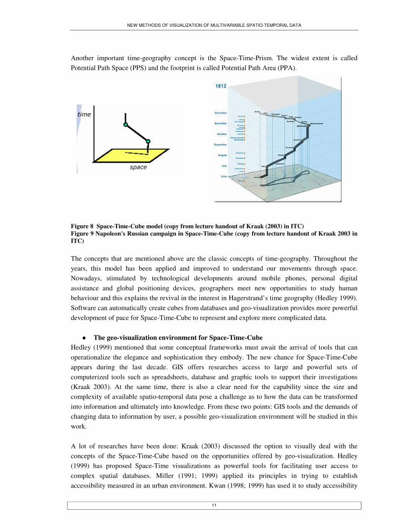
Another important time-geography concept is the Space-Time-Prism. The widest extent is called Potential Path Space (PPS) and the footprint is called Potential Path Area (PPA).
Figure 8 Space-Time-Cube model (copy from lecture handout of Kraak (2003) in ITC) Figure 9 Napoleon's Russian campaign in Space-Time-Cube (copy from lecture handout of Kraak 2003 in ITC) The concepts that are mentioned above are the classic concepts of time-geography. Throughout the years, this model has been applied and improved to understand our movements through space. Nowadays, stimulated by technological developments around mobile phones, personal digital assistance and global positioning devices, geographers meet new opportunities to study human behaviour and this explains the revival in the interest in Hagerstrand’s time geography (Hedley 1999). Software can automatically create cubes from databases and geo-visualization provides more powerful development of pace for Space-Time-Cube to represent and explore more complicated data.
� The geo-visualization environment for Space-Time-Cube Hedley (1999) mentioned that some conceptual frameworks must await the arrival of tools that can operationalize the elegance and sophistication they embody. The new chance for Space-Time-Cube appears during the last decade. GIS offers researches access to large and powerful sets of computerized tools such as spreadsheets, database and graphic tools to support their investigations (Kraak 2003). At the same time, there is also a clear need for the capability since the size and complexity of available spatio-temporal data pose a challenge as to how the data can be transformed into information and ultimately into knowledge. From these two points: GIS tools and the demands of changing data to information by user, a possible geo-visualization environment will be studied in this work. A lot of researches have been done: Kraak (2003) discussed the option to visually deal with the concepts of the Space-Time-Cube based on the opportunities offered by geo-visualization. Hedley (1999) has proposed Space-Time visualizations as powerful tools for facilitating user access to complex spatial databases. Miller (1991; 1999) applied its principles in trying to establish accessibility measured in an urban environment. Kwan (1998; 1999) has used it to study accessibility
NEW METHODS OF VISUALIZATION OF MULTIVARIABLE SPATIO-TEMPORAL DATA
12
differences among gender and different ethnic groups. She also started integrating cyberspace into the cube. Forer (1998) has developed a interesting data structure based on taxels (‘time volumes’) to incorporate in the cube to represent the Space-Time-Prism. From a visualization point of view the graphics created are often of an ad-hoc nature (Kraak 2003). The key words of the geo-visualization environment are interactive, dynamic visualization and alternative views. These characteristics can offer the user a full flexibility to view, manipulate data, and query data. Interaction is needed because the three-dimension cube has to be manipulated in space to find the best possible view (Kraak 2003) i.e. view the cube from different direction, and it should be possible to query the cube’s content. Time is always present in the Space-Time-Cube which automatically introduce dynamics (See figure 10). Alternative graphics can appear outside the cube and are linked and should stimulate thinking new insight and explanations. Based on the above literature review on STC (Kraak 1999, 2001, 2003; Hedley 1999; MacEachren 1994 etc.), the following functions are identified to be useful in visualization multivariable spatio-temporal data in this research:
� Option to move slider planes along each of axes � Highlight a period (location, time) � X,Y axes are represented by other variable � Link other view with other graphic � Drag reference into the cube to measure time or location � Switch on or off the footprint or the plane in a certain time � Rotating the cube independently, get the different view. � Spinning option for automatic rotation � Zoom in and zoom out � Selection of segments � Define query � Multimedia combination
These functions will be the options for prototypes that are developed in the research. However, one rule must be followed: the functions are all based on the questions: what tasks are expected to be executed when working with a Space-Time-Cube. The relation between question and the Space-Time-Cube will be discussed in the following.

NEW METHODS OF VISUALIZATION OF MULTIVARIABLE SPATIO-TEMPORAL DATA
13
Animation map
Figure 10 Animation in Space-Time-Cube
� Relation between Space-Time-Cube and questions based on the model of spatio-temporal data
The reason why this topic must be discussed here, because the functions are all based on the notions: what questions are expected to be answered when working with a Space-Time-Cube? (See figure 11). After analysing the questions about spatio-temporal data and the kind of questions that can be answered with the Space-Time-Cube, further study is on the possibility of the Space-Time-Cube to visualize multivariable spatio-temporal data. Figure 11 Design the Function Based on question As mentioned before, most of questions about spatio-temporal data can be described through the elementary model of spatio-temporal data that come from Peuquet (1994) (see figure 2). Figure 3 extended of Peuquet’s Concept to describe multivariable spatio-temporal data as “what”, “when”, “where” and “how”. This section will analyze the questions about spatio-temporal data by these three elements at first. Furthermore the potential solution in Space-Time-Cube to represent multivariable spatio-temporal data will be discussed. Figure 12 The corresponding relationship between Space-Time-Cube and three components concept from Peuquet (1994)
What
Where
When
Form Concretion Base on Question Tasks Function Environment

NEW METHODS OF VISUALIZATION OF MULTIVARIABLE SPATIO-TEMPORAL DATA
14
In a Space-Time-Cube, the Z axis answers “when” always, the object in the Space-Time-Cube indicates “what”, and X,Y forms the 2-dimension space which indicates “where” (see figure 12). Corresponingly, the problems about spatio-temproal data can be dealt with as follows:
� When+what�where The question is where the object at a certain time point is. This question can be represented in the Space-Time-Cube as: what is the value of (x, y) at a certain time (the black line in figure13 shows the processes for this question). The corresponding process in the environment of Space-Time-Cube can be: move the mouse over the trajectory of the object, its corresponding time value will be shown at Z axis, and then stop and click at the desired time point, the corresponding location of point will be shown both at 2D and 3D views, and the X and Y coordinate value will be shown in 2D map. The 3D view can help the user visualizing the relationship between the time and space. At the same time, 2D view helps the user in orientation and navigation because 2D map is the familiar way for people to obtain the geo-information. Figure 13 “When+what����where” (the black line) and where+what����when (the red line) in Space-Time-Cube
� Where+what�when The question is about when an object is at a certain place. The question can be represented as what time the object in the cube is at a certain place (see figure 13, the red line indicate the process). The correspond process in the environment of Space-Time-Cube can be: move the mouse over the trajectory of the object, the corresponding x, y value will be shown both at 2D and 3D view, stop and click at the desired place, the corresponding time point value will be shown at Z axis.
� When+where�what The question is about what exists at a certain place at a certain time point, or what takes place at a certain place at a certain time point. The corresponding function can be query (T1=08:00, Space1=(X1, Y1), object1_id=?). Then the object or event is highlighted in cube.
� Where�when+what The question is about at a certain location, what happened with the time. This location in cube base can be area or point. The function can be that selecting the area or the point in cube base, the information about it through time will be shown in a table. Especially, if it is an area, the different view from the bottom to top, the change information about the area will be shown. The classic
X0
Y0
X0
T0

NEW METHODS OF VISUALIZATION OF MULTIVARIABLE SPATIO-TEMPORAL DATA
15
example is the enlarging of a city. In figure 14, the red line indicates the location of interest. The blue and the green lines indicate the trajectory of objects. Through defining the interested location (the red line), the intersection points are the result and the object and time which identify the intersection will be shown in table. (see the figure 14) Figure 14 What did appear at the certain location
� When�where+what The question is about what the situation at certain moment is. The process can be: click a time point which is wanted, then the plane at that certain time will be shown in 2D view. At the same time the plane can be animated to fly through the Space-Time-Cube and unwrap it in the 2D view. This help users to get sense about where each view comes from, what the relation between 3D and 2D is (see figure15). Figure 15 What is the location of the objects at a certain time (extract a time plane in Space-Time-Cube)
� What�when+where The question is about what the change of an object is at both time and space scope. The function about it can be: click the object of interest in the cube, only the trajectory which is chosen is highlighted or is shown in another Space-Time-Cube. At the same time, all the information about this object is shown in table views.
T0
B
A
X0

NEW METHODS OF VISUALIZATION OF MULTIVARIABLE SPATIO-TEMPORAL DATA
16
As mentioned before, another important concept about spatio-temporal data comes from Andrienko, Andrienko (2003). They classified spatio-temporal data according to the kind of changes occurring over time, the corresponding view in Space-Time-Cube will be discussed in more detail:
� Existential changes: appearance and disappearance. The Existential changes can be represented by the three components as where+when�what. In Space-Time-Cube, the existential changes are show at the start and stop point of trajectory. The typical example is archaeology which is discussed by Kraak (2004) . The location of a find will be presented be a vertical line, so the duration, start point and end point of this find are shown clearly in Space-Time-Cube.
� Changes of spatial properties: location, shape and/or size, orientation, altitude, height gradient and volume.
This kind of change can be represented by the three components as what�where+when. In Space-Time-Cube this kind of changes can be shown perfectly, because this change base on time and space, and the Space-Time-Cube is combination of space and time just. However, the height gradient and volume can not be shown due to the third dimension representing the time.
� Changes of thematic properties expressed through values of attributes: qualitative changes and changes of ordinal or numeric characteristics (increase and decrease).
This change related to the “when+where�what” which is mentioned before, but in this case, not only the object itself, but also the characteristics of this object are considered. Some solutions are discussed base on Space-Time-Cube.
o Colour (hue and value) can represent characteristic of the object, but the value of this characteristic should be nominal, ordinal measurement scale.
o Size can be used to represent ratio or interval data in Space-Time-Cube, for example, in PPS (Potential Path Space), the thickness of the line can represent the load factor of the person.
o Sound can supply information of one variable about the object. The mouse click the object in Space-Time-Cube, the voice which is defined before and represents corresponding value of the certain variable of the object at that time will ring.
o Interactive visual environment will be proposed with an emphasis on alternative graphic that are connected the cube via multiple link views. It includes almost all function which is provided by geo-visualization, such as X, Y be represented by other variable, link the view with other graphic etc. It will be discussed again later.
o Chernoff face is a visualization solution for multivariable data will be discussed in section2.3.2.3. It is uses the feature of a human face to show different variables. It is good at giving an impression about the state of the object, especially the state of a person because the expression is a gift to human being and is familiar to people. The position of the faces can show the state of the multivariable belonging to whom (the trajectory of object) or where. In the Space-Time-Cube, an object is a point at a time and the position of the point indicates the geo-location of the object. As mentioned before, a simple rule, which is used to represent multivariable spatio-temporal data, is that at a particular time, an object exists at one location with a state. Based on this rule, a face is put at a point which indicates the corresponding time and geo-location

NEW METHODS OF VISUALIZATION OF MULTIVARIABLE SPATIO-TEMPORAL DATA
17
t
X
Y
variables. It is impossible to put a face on each point of the trajectory. Once the state changes, a new face which represents the current state of the object is put on the point on the corresponding position. In this way, the change is highlighted and easy to discover. The line segments which have no face on it represent the duration which maintain the last state. Figure 16 shows an example of using Chernoff face in Space-Time-Cube.
Figure 16 Chernoff face in Space-Time-Cube
� Advantages of Space-Time-Cube Space-Time-Cube provides the following advantage for representation spatio-temporal data.
o Space-Time-Cube is a natural combination of time and space (they are inseparable). The relation between time and space can be viewed all the time. All the basic questions about Spatio-temporal data can be addressed in Space-Time-Cube.
o It is good at studying individual movement or change with time, and it gives a direct view about the speed of object, the trajectory of object and the geographic characteristic of movement.
o The time scale exists all the time, time is emphasized, and both continuous and discrete time can be represented. At the same time it is possible that different time variables exist and one should be selected by the user. For instance time could be given in years but also according particular history events like the reign of an administration.
o Because the Space-Time-Cube provides an integration view for spatio-temporal data, it is a good interface to explore the geo-spatial data (Kraak 2003).
� Disadvantages of Space-Time-Cube
o In Space-Time-Cube, using existing method, it is difficult to represent multivariable data with time. As mentioned before, only five items can be used to represent the variables. It is difficult to crush this limitation for original Space-Time-Cube.

NEW METHODS OF VISUALIZATION OF MULTIVARIABLE SPATIO-TEMPORAL DATA
18
o When using the Space-Time-Cube to represent multivariable spatio-temporal data with colour, sound etc, only nominal data can be represented. It is difficult to represent higher level information.
o The height and gradient of 3D object are difficult to represent in Space-Time-Cube
2.3.2. Visualization for multivariable data
An object is multivariable by nature, because an object always exists with a lot of characteristics. Research on the changes of these characteristics is very important, because accumulation of the changes in quantity leads to a change in quality. How can people get the detailed information about object changes and the kind of characteristics that influence the object? What are the relationships among these characteristics of an object? How do these characteristics interact? New technology and methodology offer more options to study the characteristics of objects, for example: database, geo-visualization, computer display etc. In database, these characteristics can be represented as multivariable or multi-attribute data. The reason why people study these multivariable data is to find valuable information hidden in the data. Visualization is an effective tool to reveal pattens and trends. Visualization supplies a visible view to people who study these multivariable data. Consequently, they may get information in which they are interested. Graphics are introduced to study multi-variable. There are all kinds of graphic options, and the following gives a summary of these graphics, which are current classic and popular ones, in four aspects, basic concepts, temporal components, advantages, and disadvantages.
2.3.2.1. Simple graphs
Simple graphs are the most popular tool to support the data visualization. Most people are familiar with simple graphs such as bar chart, pie char, and x-y plots. They are intuitive and easy to use.
� Temporal component However, for the simplest graphs, there is no effective method to deal with multivariable data and with the time issue. The common way is to use more graphs. Some simple graphs are used to represent time, for example, bar chart which uses x-axis to represents time, y-axis to indicate value of a certain attribute, but it is difficult to represent the relation between variables with time.
� Advantages o It is simple and easy to understand, because it is a common representation for people. o It can be built easily with popular software.
� Disadvantages
o Show highly aggregated data and actually present only a very small number of data values (as in the case of bar charts or pie charts)
o Have a high degree of overlap which may occlude a significant portion of the data values (as in the case of X-Y plots)
o It is limited to represent the relationships between different attributes (as in the case of bar charts) (Keim 2002)

NEW METHODS OF VISUALIZATION OF MULTIVARIABLE SPATIO-TEMPORAL DATA
19
������ ��� ��� ���
���������������
��������������������
� What can be done further
For an analysis of large volumes of multivariable spatio-temporal data, what is needed is to present an overview of the data but at the same time show the detailed information for each data item (Keim 2002). Simple graphics are easy to link to the Space-Time-Cube, so the overview of the data is presented in Space-Time-Cube, and the detailed information is shown in simple graphics. At the same time, the graphic can change with the slider of z-axes (time) of Space-Time-Cube, and then a dynamic link will be built.
2.3.2.2. Parallel Coordinates Plots (PCP)
Parallel Coordinates Plots (PCP) (Inselberg 1985) are effective to deal with multivariable data. The observation are represented on a PCP as series of line segments, passing through parallel axes, each of which represents a different variable. Each line passes through an axis at a location that indicates the observation’s value relative to all other values. The ends of the axis represent the maximum and minimum values of the axis variable for all observations under consideration. The result is a multivariate signature for each observation, and a visual representation of relationships among many variables (figure 17). Figure 17 Parallel Coordinates plot This is the basic concept of static PCP; however a dynamic, interactive and customized version of the PCP is well suited for the type of expert-driven detective work necessary for the exploration of large spatial and spatiotemporal database. This technology in geo-visualization is characteristicized by highly interactive representations designed for use by individuals, expert in the understanding of the mapped phenomenon, for exploratory analysis purposes (Edsall 2003). For example, the interactive environment allow user to assign a variable to any axis, so user can change the order of the axis which represent the interesting variables (Brodbeck 2003). Focusing in the PCP removes the lines of all other observation from display to reduce the visual clutter and draws the focused observation as highlighted line. It can be used to deal with the problem of line density in the PCP. And the EDA (exploratory data analysis) concept of brushing can be used also. Brushing consists of highlighting a group of data observations by some method of selection; in a PCP, multiple line segments may be selected simultaneously by click-dragging a box around the bundle.

NEW METHODS OF VISUALIZATION OF MULTIVARIABLE SPATIO-TEMPORAL DATA
20
� Temporal component
There are three methods to represent the time dimension in PCP. First, a single axis can serve as a time axis because time is at least an ordinal-level variable. Minimum and maximum attribute values are plotted individually along each axis. Second, again time is plotted as parallel axes, but the values along each axis are standardized. This variation is required to visualize temporal trend, as long as the scales from axis to axis remains the same (figure18 (Edsall 2003)). It is to say that the maximum and minimum values of the entire time series would define the ends of the axes that represent the variables. The last methods, assign each polyline which represents one object to a specific object at the specific time. For example, if states of one object at 5 time point should be represented, then the object will be represented as 5 lines instead of one line. If you want to view M objects at n time points, there will be M*n polylines be showed in the PCP. However it is difficult to identify which lines indicated the same object and too many polyline will be shown.
Figure 18 Typical axis value designation hides temporal trends (left). Axis values that are consistent across time axes reveal temporal features (e.g., most observations reach their minimum temperature at 6:00 am right). In fact, the first and the second methods mentioned before are based on the same concept: it uses different axes indicate the different time points. Two problems appear, first, the time is continuous, but the representation is discrete. There will be too many axes if you want to represent multivariable at many time points. Second, the relation between variables with time cannot be represented. The standard PCP uses different axes to represent multivariables. For time issue, the axes are used to represent different time point. If there are disadvantages when you combine them in parallel direction, why not combine them in vertical direction in a 3D model. This will be further discussed in chapter 3.
� Advantages o PCP is not only useful but also necessary when the data sets are large and
multivariable o The relationships among variables can be shown clearly o When the data sets are completely unknown and unrecognizable, the patterns of
interest can be extracted without the aid of computational algorithms. o Any number of the variables can be represented in PCP.
� Disadvantages:
NEW METHODS OF VISUALIZATION OF MULTIVARIABLE SPATIO-TEMPORAL DATA
21
o The sheer number of observations and variables in a large (geo-graphic) database quickly overloads the representation to the point where very little information can be perceived and extracted. This can be dealt with by interactive, dynamic PCP partly.
o The order in which the axes are linked up clearly influences the amount and quality of the insight gained from the representation(Keim 2002). It is to say that the relationships among a small number of variables would be difficult to discern if those variables were distant from one another on the representation, this can be overcome by interactive PCP.
o It is necessary to reduce position in space to one dimension. Use one axis to represent one location by name, or use two axes to represent the X, Y. However, it is difficult to give the feeling about the relative position.
o It is difficult to represent the relationship of these variables with time.
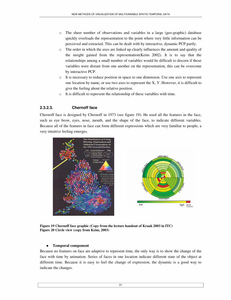
2.3.2.3. Chernoff face
Chernoff face is designed by Chernoff in 1973 (see figure 19). He used all the features in the face, such as eye brow, eyes, nose, mouth, and the shape of the face, to indicate different variables. Because all of the features in face can form different expressions which are very familiar to people, a very intuitive feeling emerges. Figure 19 Chernoff face graphic (Copy from the lecture handout of Kraak 2003 in ITC) Figure 20 Circle view (copy from Keim, 2003)
� Temporal component
Because no features on face are adaptive to represent time, the only way is to show the change of the face with time by animation. Series of faces in one location indicate different state of the object at different time. Because it is easy to feel the change of expression, the dynamic is a good way to indicate the changes.

NEW METHODS OF VISUALIZATION OF MULTIVARIABLE SPATIO-TEMPORAL DATA
22
� Advantage o It gives a person a very intuitive feeling at once. It is good at presenting the variables. o It is adaptive to represent the like/dislike, health situation, costing situation, and
income situation, because the expression indicate these situation in a nature way.
� Disadvantage o Due to the limited the number of features on the face, only a few variables can be
represented. o Only probable feeling can be shown, detailed information such as numbers can not be
indicated.
2.3.2.4. Circle View
The basic idea of circle view display is to divide a circle into a number of segments (see figure 20) , depending on the number of dimensions of the data set (the number of variables). Each segment is then divided in sub-segments in order to visualize the distribution and changes of the time dependent data. Time is represented as the radius from the centre of a circle to the edge of the circle. The colour of each sub-area shows the value of an attribute at a certain point in time.
� Temporal component Circle View display provides more space for the time slots of actual time events, see figure 22 for an illustration of this idea. One can easily see, that the actual time event is t9 the oldest time event is t0. The length of the corresponding time slot, defined by the start radius and the end radius depends on the priority of the events in time (Keim 2003). Figure 21 Time reference in circle view (copy from Keim 2003)
� Advantage o It is useful to visualize correlations in the data and compare different attributes at a
certain point in time. o It is can visualize the multivariable temporal data. o It is good to identify patterns, exceptions and similarities in the data. o It is easy to understand.

NEW METHODS OF VISUALIZATION OF MULTIVARIABLE SPATIO-TEMPORAL DATA
23
� Disadvantage o Each circle indicates one object, so more objects need more circles to represent. Then
the relations between different objects with time are difficult to view. o Colour is used to represent the value of the object in certain attributes. If the range of
the value in different attributes is different, it is meaningless to show the values in different variables. At the same time, certain values (interval or ratio data) are difficult to represent.
2.3.2.5. PBC (Pixel bar charts)
The basic idea of PBC is to use the intuitive and widely used presentation paradigm of bar charts, but also to use the available screen space to present more detailed information. By colouring the pixels with the bars according to the values of the data records, very large amounts of data can be presented to the user. To make the display more meaningful, two parameters of data records are used to impose an ordering on the pixels in the x- and y- directions. Pixel bar charts can be seen as a generalization of bar charts visualization. They combine the general idea of x-y plots and bar chart to allow an overlap-free, non-aggregated display of multi-attribute data. Figure 23 shows an example of PBC.
� Temporal component For a general definition of pixel bar charts, one need to specify the dividing attributes, the order and colour of attributes. The most potential attributes to indicate the time is use it as dividing attributes, for example, X-(see figure 22-b). In this case, PBC visualizes each data item without aggregation and allows the ordering of the data items belonging to more than one attribute.
Figure 22 Pixel bar charts Another potential way is series PBC, and each PBC indicates the situation in one time point. These series PBC can form dynamic view, of are combined together. Space-Time-Cube can combine them, but because the cube is 3D object, the pixel within the cube is not easy to view because it impossible to view the core of solid cube.
� Advantage
o PBC can focus on certain attribute range, and identify the distribution of attribute values of specific subsets of the data.
o Show patterns, correlations an trends between small subsets of the data.
(a) (b)

NEW METHODS OF VISUALIZATION OF MULTIVARIABLE SPATIO-TEMPORAL DATA
24
o Allow user to access detailed information, e.g. about single customers.
� Disadvantage o It is difficult for common people to understand. o For generating the PBC visualizations, one has to solve a complex optimization
problem. o It is difficult to represent time issue.
2.4. Summary
Designers are discovering how to use rapid and high-resolution colour displays to present and manipulate large amounts of information in compact and user-controlled ways (Plaisant 2004). Not only all kinds of old graphic models get a new development room: the geo-visualization environment, but also new models for data visualization are powerful supported by a geo-visualization environment. However, existing visualization methods for spatio-temporal data and multivariable data, can sometime not represent the multivariable spatio-temporal data. However, there exists a potential chance to combine the graphic with the Space-Time-Cube to visualize multivariable spatio-temporal data. Based on the discussion before, the PCP is the most potential method to combine with Space-Time-Cube. The PCP is 2D graph and the Space-Time-Cube is 3D, but the third dimension is defined as time reference always. The other two dimensions in 3D can be changed to PCP graphic. Both the multivariable and time of object can be represented. This geo-visualization tool can be used to give clearer view on the hierarchy between data. Second, the option for X and Y axes of 3D graphic may provide more interactive function for user to make they interested. These will be further discussed in next chapter.

NEW METHODS OF VISUALIZATION OF MULTIVARIABLE SPATIO-TEMPORAL DATA
25
3. Models design
3.1. Introduction
As described in chapter two in this research, multivariable spatio-temporal data is used to describe the characteristics. Based on the model of Peuquet (1994), four components are distinguished in multivariable spatio-temporal data: space (where), objects (what), time (when) and multivariable (how) in this research (see figure 3 and 4). The questions mentioned in last chapter, are used as the starting point to study existing visualization solutions and will be the key factor to design the models described in this chapter. As mentioned in section 2.3, the existing visualization solutions are good at representing either spatio-temporal data or multivariable data, but not both together. After analysing the potentials of the combination of the Space-Time-Cube and several multivariable graphics, the new models: Multivariable-Time-Cube, PCP-Time-Cube, are proposed and designed to visualize the multivariable spatio-temporal data in this chapter.
3.2. Multivariable-Time-Cube
3.2.1. Why Multivariable-Time-Cube
In chapter 2, the visualization solutions for the changes of attributes value, are discussed briefly, colour, size, Chernoff faces and sound can be used to visualize the multivariable changes in the Space-Time-Cube. Two problems appeared: the number of the variables that can be represented is very limited and the type of the variables should be nominal, e.g. certain values can not be viewed clearly. However, geo-visualization offers the possibility to use the concept of the Space-Time-Cube to visualize multivariable spatio-temporal data. The original Space-Time-Cube is used to visualize spatio-temporal data and all the questions on the spatio-temporal data can be addressed, except that the “how” question cannot be properly addressed. Temporal variable can be represented along the Z-axis because temporal data is one dimension and time points or a continuous time can be represented. Another cube that has the same time reference as the original Space-Time-Cube: on the Z-axis, but uses X and Y to represent other user-defined variables, is introduced to visualize the multivariable data with time. It can be called Multivariable-Time-Cube. Therefore, an emphasis is placed on spatial, temporal, and attributes relationships, and the concept of multivariable spatio-temporal data can be well applied by linking the classical Space-Time-Cube to another cube or graphic. In other words, based on the model of multivariable spatio-temporal data, a classical Space-Time-Cube is used to represent “what”, “when” and “where” components (the triangle left in figure 23), and the cube can be linked to Multivariable-Time-Cube which represent the “how”: multivariables with time (the polygon on the right). Based on this idea, several cubes, which are defined by different variables with X and Y axes can be linked to represent

NEW METHODS OF VISUALIZATION OF MULTIVARIABLE SPATIO-TEMPORAL DATA
26
multivariable data with time. The cube whose X and Y axes are defined by multivariables called a Multivariable-Time-Cube. Figure 23 Multivariable-Time-Cube and multivariable spatio-temporal data model
3.2.2. Multivariable-Time-Cube model
The classical Space-Time-Cube is the basis and other cubes and graphics are linked by time reference. To link these cubes, a synchronism link is needed. As mentioned before, the movement of an object in Space-Time-Cube is visualized as a trajectory. In Multivariable-Time-Cube, an object is represented also as a trajectory, which indicates the value change of the variables which are defined on the X and Y axes, and the slope of the trajectory indicates the speed of the change. In Space-Time-Cube, at a certain time, an object is a point which indicates the position according the geo-space reference and time reference. Similarly, at a certain time, the object is also a point in Multivariable-Time-Cubes, and
Multivariable-Time-Cube
Space-Time-Cube
Graphic
�����������
����
���
���
������
������
���
��How

NEW METHODS OF VISUALIZATION OF MULTIVARIABLE SPATIO-TEMPORAL DATA
27
the position of this point indicates the value of the object for the two variables which are defined at that time. It should be mentioned that, in Space-Time-Cube the X and Y axes form a continuous space, and the X, Y variables are inseparable. However, in Multivariable-Time-Cube, the X, Y axes can be defined as any variable, so the relationship between the two axes may be meaningful or may not, and it is user-defined. Figure 24 shows an example of Multivariable-Time-Cube. The yellow cube is a Space-Time-Cube, and the green one is a Multivariable-Time-Cube. The red and blue lines indicate object, the same colour indicates the same object, and the red vertical strip indicates time synchronism reference. Figure 24 Multivariable-Time-Cube model The result of projecting the trajectory on the bottom in Space-Time-Cube is the footprint of an object path (See figure25-a). However, in Multivariable-Time-Cube, the projection of the trajectory on the bottom, side and back surface are also meaningful. The projection on the bottom shows how the variables of the object change during the period of the path and the relationship between the two variables in two axes. Figure 25-b shows that the projection of the trajectory as a polyline which indicates the change of the variables. The polyline is formed by several sections. The slope of the sections indicates the decrease or increase of the variables, and the speed of the change can be viewed also by the gradient of line in this graphic. A vertical or horizontal section indicates that the variable doesn’t change. In addition, sometime the object in Multivariable-Time-Cube is a point and therefore a point is also projected on the bottom. The relevant position of the point to the whole polyline indicates the state of the object about the two variables at that time. Figure 25-c shows the trajectory projection on the left surface, and it indicates how the V1 variable changes with time. The slope of the line indicates the speed of the changes, and the red small circle shows the situation of the object about V1 at a certain time. Figure 25-d shows the trajectory projection on the back surface and it shows how the V2 changes with time.
t
X
Y
v2
v1
t
t
Space-Time-Cube Multivariable-Time-Cube

NEW METHODS OF VISUALIZATION OF MULTIVARIABLE SPATIO-TEMPORAL DATA
28
Figure 25 Projection graphic in Space-Time-Cube and Multivariable-Time-Cube How to use this model to answer the multivariable spatio-temporal data questions? The rest of this section discusses how the classical simple questions about multivariable spatio-temporal data, which are mentioned in section 2.2.2., are addressed in Multivariable-Time-Cube model and how more complex combinations of the simple questions are possible.
3.2.3. Questions about multivariable spatio-temporal data in the Multivariable-Time-Cube
3.2.3.1. When���� where+ what+ how
Using the time as the synchronism link, the question when�what + where +how can be answered. After identification of a certain time at the synchronism axis (see the red line between the two cubes in fig. 24), the corresponding time planes (the two white horizontal planes infig.24), that identify “when”, will be highlighted in the two cubes. The intersection points of the trajectories with the time plane in Space-Time-Cube indicate the locations of the objects at certain time and the intersection points of trajectories with the time plane in Multivariable-Time-Cube indicate the values of the objects for the two variables at the same time. Moving the slide of the synchronism axis results in a corresponding time plane that will be highlighted, and the corresponding intersection point will be obtained. Furthermore, the point of the projection in a 2D view like the small circles in each 2D graph in fig. 25) show the situation and the location of the objects at that time. The information about “where” can be viewed at Space-Time-Cube. At the same time, the information about multivariable with time can be found in Multivariable-Time-Cube. It is just like: where+what����when����how+what.
V1
V2
V1
t
V2
t
(a) (b)
(c) (d)
How Where
What
When

NEW METHODS OF VISUALIZATION OF MULTIVARIABLE SPATIO-TEMPORAL DATA
29
3.2.3.2. What ���� when+ where+ how
Using the object as the synchronism reference, the question what�where+ when +how can be answered. The object in both Space-Time-Cube and in Multivariable-Time-Cube is a trajectory (polyline), and the two trajectories, which identified same object, are linked with the synchronism axis. When the slide is moved along the synchronism axis, the corresponding polylines in two cubes will be highlighted. Another way is choosing the object in Space-Time-Cube or in Multivariable-Time-Cube; the corresponding object will be highlighted in the other cube at the same time.
3.2.3.3. Where���� when+ what+ how
Location cannot be found via the synchronism link because “where” only exists in Space-Time-Cube. However, this question can be answered by using “when+what” via the synchronism link. It means that starting from a location, the question about where�when+what will be answered in Space-Time-Cube at first, and the corresponding results is sections of trajectory which identify “what+when”. Then the “when+what” will be translated to Multivariable-Time-Cube as the synchronism link, and the question of “what+when�how” will be answered in Multivariable-Time-Cube. The steps are shown as red arrow in Figure 26. Figure 26 The steps of answering the question of where���� when+ what+ how The detailed implementation is: after a location (a point or area) is identified in 2D map view (the reason why choosing the 2D map is that it is easy to operate), the corresponding geo-information will be passed onto the basic cube. In Space-Time-Cube, there exists relationship between the object and the location, (be inside or not). The list about “when’ and “what” will answer the question about what and when the object exists or passes through the identified area. Based on the information about the “when +what”, the corresponding multivariable information will be shown as highlight points or
How Where
What
When
How Where
What
When
MTC STC
Where
Where�when+what when+what�how
How
When+what
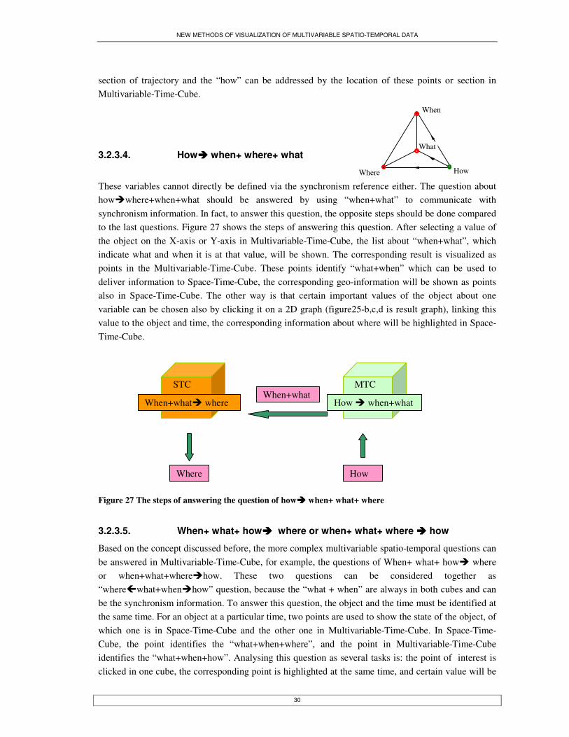
NEW METHODS OF VISUALIZATION OF MULTIVARIABLE SPATIO-TEMPORAL DATA
30
section of trajectory and the “how” can be addressed by the location of these points or section in Multivariable-Time-Cube.
3.2.3.4. How���� when+ where+ what
These variables cannot directly be defined via the synchronism reference either. The question about how�where+when+what should be answered by using “when+what” to communicate with synchronism information. In fact, to answer this question, the opposite steps should be done compared to the last questions. Figure 27 shows the steps of answering this question. After selecting a value of the object on the X-axis or Y-axis in Multivariable-Time-Cube, the list about “when+what”, which indicate what and when it is at that value, will be shown. The corresponding result is visualized as points in the Multivariable-Time-Cube. These points identify “what+when” which can be used to deliver information to Space-Time-Cube, the corresponding geo-information will be shown as points also in Space-Time-Cube. The other way is that certain important values of the object about one variable can be chosen also by clicking it on a 2D graph (figure25-b,c,d is result graph), linking this value to the object and time, the corresponding information about where will be highlighted in Space-Time-Cube. Figure 27 The steps of answering the question of how���� when+ what+ where
3.2.3.5. When+ what+ how���� where or when+ what+ where ���� how
Based on the concept discussed before, the more complex multivariable spatio-temporal questions can be answered in Multivariable-Time-Cube, for example, the questions of When+ what+ how� where or when+what+where�how. These two questions can be considered together as “where�what+when�how” question, because the “what + when” are always in both cubes and can be the synchronism information. To answer this question, the object and the time must be identified at the same time. For an object at a particular time, two points are used to show the state of the object, of which one is in Space-Time-Cube and the other one in Multivariable-Time-Cube. In Space-Time-Cube, the point identifies the “what+when+where”, and the point in Multivariable-Time-Cube identifies the “what+when+how”. Analysing this question as several tasks is: the point of interest is clicked in one cube, the corresponding point is highlighted at the same time, and certain value will be
How Where
What
When
MTC STC
Where
When+what� where How � when+what
How
When+what

NEW METHODS OF VISUALIZATION OF MULTIVARIABLE SPATIO-TEMPORAL DATA
31
shown in identify window. To view the relevant position with whole movement and change, two cubes can supply this kind of overview; to view the exact value the identify window or 2D graph will supply this detail. If the point which is in the Space-Time-Cube is selected, the question about ‘when+ what+ where�how” will be answered by the corresponding point in Multivariable-Time-Cube. If the point is selected in the Multivariable-Time-Cube, the question about “when+ what+ where �how” will answered by the corresponding point in Space-Time-Cube. The projections which are mentioned before can make it easier to understand information about the situation of the object at certain time with whole change or movement. The user will start by finding one interested point which is either in Space-Time-Cube or in Multivariable-Time-Cube, the point will show other information about the object at that time. Furthermore, by clicking the point in the 2D view, the corresponding point will be highlighted in the cubes and 2D map also. The points which are identified as same object at the same time in all the cubes and the 2D project graphics will be linked together to show multivariable information and spatio-temporal information.
3.2.4. Design of interfaces and functions for Multivariable-Time-Cube
Based on the above analysis of the questions that should be answered in Multivariable-Time-Cube, a user interface environment will be designed. The reason why this topic is discussed here is that an interactive environment is required for the user to understand and operate Multivariable-Time-Cube. The prototype of Multivariable-Time-Cube and its interface will be discussed in more detail in next chapter. Figure 28 shows a draft interface of Multivariable-Time-Cube.
Figure 28 Draft interface of Multivariable-Time-Cube �
STC
MTC1
MTC2

NEW METHODS OF VISUALIZATION OF MULTIVARIABLE SPATIO-TEMPORAL DATA
32
3.2.4.1. Option function
Options provide more freedom for users to create their favourite view. In this model, several options are available.
• User can define how many cubes will be shown together. One cube is always the basic Space-Time-Cube, the others are Multivariable-Time-Cubes.
• Based on the number of multivariable-Time-Cubes, the corresponding cubes will be created, and the options for axes of these cubes are available. It is to say, the Z-axis is the time reference by default, the attributes name for X and Y axes will be listed in each Multivariable-Time-Cube. Hence the user can select attributes on each axis in Multivariable-Time-Cube.
• User can choose the synchronism link. • For different cube, colour, size and texture can be used to represent different variables of
interest.
3.2.4.2. 3D view
Based on the defined options, 3D view for Space-Time-Cube and Multivariable-Time-Cubes will be created. The 3D view is used to show the -Time-Cube and Multivariable-Time-Cubes. The interactive tools are designed as follows.
• User can change views, by revolves cubes, using zoom in and zoom out tools • User can click a point on a trajectory which identifies an object, and corresponding trajectories
in other cubes will be highlighted. • User can click a point on the X, Y and Z axes to extract a projection plane, the plane will be
shown in 2D view. • Each point of an object in both Space-Time-Cube and Multivariable-Time-Cube indicates the
exact value about “when +what+ how” or “when +what+ where”. So the corresponding value will be shown when the mouse point to the point.
3.2.4.3. 2D view for geographic map
To locate the positions of the objects, the most familiar method for user is 2D map, so user can select whether the map is shown in 2D view. 2D views are also used to show the projection of the trajectories in Multivariable-Time-Cube. The object which is identified with “what+when” or “what” only, the corresponding points or the polyline will be highlighted in 2D view also. Furthermore, the user can define the study area in 2D map, then a list of corresponding where �what + when +how appears and the sections of the trajectories which are in the identified area will be highlighted.
3.3. PCP(parallel coordinates Plots)-time cube
3.3.1. Why PCP-Time-Cube
As mentioned before, Space-Time-Cube is an effective method to visualize spatio-temporal data. The movement of object, in Space-Time-Cube, is visualized as a trajectory following the time, which is a

NEW METHODS OF VISUALIZATION OF MULTIVARIABLE SPATIO-TEMPORAL DATA
33
classic model, better known as Space-Time-Path. It is the start of a people based-perspective (Miller 2003). Parallel Coordinate Plot (PCP) (Edsall 2003) can represent multivariable objects. The variables relationship among objects can be viewed also. An object is represented as a polyline crossing the normalized vertical lines representing the variable (see section 2.3.2.2, Figure 17). Along the polyline, the value about the object for different variables can be addressed. The emphasis of this visualization solution is on multivariables of the objects. In both Space-Time-Cube and PCP-Time-Cube an object is represented by a polyline, and in PCP an object is also a polyline. Although the polylines have different meanings in PCP and STC (the value of an object at different attributes versus the trajectory of the object in both space and time), they identify the objects. PCP is 2D graph and the time dimension can be added to PCP. This result is called PCP-Time-Cube. Because a variable value of an object at a time is certain, “when”+“what”-+“how” is represented as a points in PCP-Time-Cube. Different points, which identify different states of an object with time, form a surface that identifies the object.
3.3.2. PCP-Time-Cube model
In PCP-Time-Cube, the X-axis represents the different variables, for instance body temperature, etc. Y-axis represents the range of the attribute values of objects in the different variables, in case of temperature 0oC-41oC and z-axis represents the time. Figure 29 show an example of basic PCP-Time-Cube model. Any horizontal plane is a classic PCP graphic to address the multivariable value for all objects at certain time; It is called T-PCP plane (in the figure 29, the pink planes indicate the T-PCP planes). Same as in PCP, one polyline indicates the value of the object about corresponding variables, it identifies one object. Any vertical plane which corresponds to a variable axis addressed a variable in time. So any information about a variable should be in this corresponding vertical plane: the V-time plane. For example, the green plane in figure 29 is called V1-time plane. The change of an object along V1 with time is visualized as a polyline which must be on the V1 time plane. The polyline on the T-PCP plane indicates the value of the object at certain time; it is called T-object-variables line. The polyline on the V-time plane indicates the change of certain variable with the time, and it is called V-object-time line. The intersections of T-object-variable lines and the V-object-time lines are vertex of the surface, and these vertexes identify a state of an object at a time: “what+when+how”. For one object, all the T-object-variable lines and the V-object-time lines form one multifaceted surface which identifies the object. Then different objects are represented as different surfaces in PCP-Time-Cube (see figure 29 the blue surface).

NEW METHODS OF VISUALIZATION OF MULTIVARIABLE SPATIO-TEMPORAL DATA
34
�� �� �� �� �� �� �� �� �� ��
��� ��� ��� ��� ���
0 100
t
Figure 29 Relationship between PCP-Time-Cube and V-time plane, T-variable plane As mentioned before, two planes are used to address the multivariable-temporal data: one is T-PCP plane which is the same as PCP graphic, and the other is V-time plane which addresses a variable with time. However, one problem that should be noticed is that the values of the line segments between the vertical lines, i.e. the variables, are meaningless in the T-PCP plane. They are only used to link all useful points to identify one object. In V-time plane, all the line segments on the polyline which identify one object are meaningful; they indicate the value of the object at different times. Therefore, in object surface, the skeleton of the surface (red line in PCP-Time-Cube, see figure 29) can also used to identify one object.
3.3.3. Questions about multivariable spatio-temporal data in the PCP-Time-Cube
Based on the concept of PCP-Time-Cube, three kinds of information about multivariable spatio-temporal data can be extracted. A diagram is added to each question below. The green point in these diagrams is the start of a question, the red point is the answer of the questions and the black point mean no answer about the component.
t1
t2 t3
V1 V2 V3 V4 V5
T1-PCP plane
V1-time plane
PCP-Time-Cube
Object surface, characterizing one object in time

NEW METHODS OF VISUALIZATION OF MULTIVARIABLE SPATIO-TEMPORAL DATA
35
3.3.3.1. When���� what + how
In PCP-Time-Cube, the Z-axis represents temporal variable. Any time scale, such as minute, hour, day, month, year etc. and any conceptual time such as events or observation times can be defined as Z-axis. To answer the question about when� what +how, a user first need to select a time point (T0) by a click on the Z-axis, then a 2D plane is extracted from PCP-Time-Cube. The 2D plane is a standard PCP graphic at “T0” time (see figure 30). All the objects are represented as polylines which indicate the value of the object for multivariables at the selected time. T-PCP plane can answer questions such as what is the relationship among the objects for different variables, which object has the highest value for a certain variable at that moment, which objects have the same value and what is the value (intersection on some variable axes) etc. Figure 30 T0-PCP plane is extracted from PCP-Time-Cube to answer when���� what+how in PCP-Time-Cube
3.3.3.2. What����when + how
In PCP-Time-Cube, a surface identifies an object and the surface can be understood as a kind of “footprint” of the object. The surface is formed by a skeleton which includes the T-object-variable lines and V-object-time lines. To answer the question about what�when + how, a surface that represents an object can be extracted, and the surface represents the change of the values of all variable of an object with time. The blue surface in figure 31 identifies one object. Following the T-object-variable line, all the multivariable information about the object at certain time can be answered, and the V-object-time line supplies the information about the changes of the object with the variables. Multivariable spatio-temporal data questions can be answered with the object surface, such as what is the maximum (minimum) value of the object for a certain variable, what time is the object at maximum (minimum) value, what is the value of the object at a certain time.
T0
��� ��� ��� ��� ���
���������������
��������������������
T0-PCP plane
How Where
What
When
How Where
What
When

NEW METHODS OF VISUALIZATION OF MULTIVARIABLE SPATIO-TEMPORAL DATA
36
Figure 31 “What” in PCP-Time-Cube is a surface shown in blue
3.3.3.3. How���� when+ what
If a vertical section is extracted from the PCP-Time-Cube at certain variable axis, this section, which is called V-time plane, will show all the information about the variable. The objects in this section are polylines also, and it indicates how this variable of the object change with time. Questions like: what is the relationship among the objects in this variable, at what time and which object has the maximum (minimum) value for this variable, when do objects have the same value about this variable (Intersection point) etc., can be answered. Figure 32 shows how V1-time plane is extracted from PCP-Time-Cube. Figure 32 V1-time plane is extracted from PCP-Time-Cube
3.3.4. “Where” in PCP-Time-Cube
In PCP-Time-Cube, it is difficult to find the “where” information, because the space reference (x, y) in classical Space-Time-Cube is replaced by the PCP reference. A potential method is using two axes of PCP to represent X, Y coordinate values, but the coordinate values provide less meaningful information about spatial relationships to user.
t1
t2 t3
V1 V2 V3 V4 V5
V1
0 1
t
V1
How Where
What
When

NEW METHODS OF VISUALIZATION OF MULTIVARIABLE SPATIO-TEMPORAL DATA
37
The second potential way is to link the PCP-Time-Cube with a 2D map that provides geo-information (the figure33), the red point in 2D view shows the corresponding position of the object at the time point which is selected and highlighted (red) in PCP-Time-Cube. Figure 33 Link 2D map with PCP-Time-Cube However, in a static map it is difficult to supply information on the movement of object. To minimizing the disadvantages of the second method, the third solution is to link the PCP-Time-Cube with the Space-Time-Cubes. (See figure 34) Figure 34 Link between Space-Time-Cube and PCP-Time-Cube The Z axes both in both the PCP-Time-Cube and the STC represent time, so it is a visible link between the two cubes. For better synchronism, they should be on the same scale. An object is visualized as a surface in the PCP-Time-Cube and as a polyline in Space-Time-Cube. At any time point, we can get the values of the variables in PCP-Time-Cube, and geo-information in Space-Time-Cube. Based on this model, all questions about multivariable spatio-temporal data can be answered. Same as in Multivariable-Time-Cube, by defining different synchronism links: “what”,”when” and “what+when”, the questions about when�what+where+how, what �when +where+how, where �what+ when +how and how �what+where+ when can be answered. Same as mentioned in section 3.2.3.5, more complex questions can be answered in PCP-Time-Cube with Space-Time-Cube. The only difference between Multivariable-Time-Cube and PCP-Time-Cube is an object is identified as polyline in Multivariable-Time-Cube and as a surface in PCP-Time-Cube. In fact, the PCP-Time-Cube
Y0
X0
A1
T0 T
NEW METHODS OF VISUALIZATION OF MULTIVARIABLE SPATIO-TEMPORAL DATA
38
provides an overview for all multivariable-temporal data. From this overview, a lot of detailed information can be extracted.
3.3.5. Design of interfaces and functions for the PCP-Time-Cube
Based on the above analysis of questions that should be answered in PCP-Time-Cube, a user defined environment will be designed. The reason why this topic is discussed here is that interactive environment is useful and necessary for user to understand and operate PCP-Time-Cube and these functions are part of my model. The prototype of PCP-Time-Cube will be based on this design, and it will be discuss more detail in next chapter. Figure 35 shows a draft of the interface of Multivariable-Time-Cube.
3.3.5.1. Option function
Options provide more freedom for user to create their favourite views. In this model, two options are available.
• Because the PCP has several Y-axes to represent different variables, a user can define how many attributes they want to represent in PCP-Time-Cube. Based on the number he enters, the corresponding options will be available. Then he can define each axis with different variables, and the sequence of the axes can be adjusted.
• The synchronism link can be defined by the user.
3.3.5.2. 3D view of PCP-Time-Cube
• Clickable and linked to 2D view After the options are set, a 3D view of the PCP-Time-Cube will be created. This cube is an interactive one and a user can click different points which are on the X-axis or Z-axis of the cube, the corresponding V-time plane or T-variable plane will be shown in the 2D view, and at the same time the selected object or layer will be highlighted. The object surface can be clicked also, and the highlighted surface identifies an object.
• Show the value automatically Each vertex of the surface indicates a value about an attribute of the object at certain time. The corresponding value will be shown when the mouse points to the vertex. The value is 4D coordinate which shows the object, variable name, variable value and time.
• Change view, Zoom in and zoom out A user can change the orientation to view the PCP-Time-Cube, and zoom in, zoom out to get different views and get more detailed information.

NEW METHODS OF VISUALIZATION OF MULTIVARIABLE SPATIO-TEMPORAL DATA
39
Figure 35 Draft interface of PCP-Time-Cube
3.3.5.3. 2D view for extracted information and geographic map
• 2D view is used to show extracting information such as V-time plane, T-variable plane, and the 2D map extracted from Space-Time-Cube. At the same time, the part shown in 2D view will be highlighted in PCP-Time-Cube or Space-Time-Cube to show the relationship of the map or graphic with the cubes. Furthermore, user can select an object in 2D graph, the corresponding object will be also highlighted in 3D view.
• To locate the position of an object, we have to use a 2D map and the user can choose whether the map is shown or not.
3.3.5.4. Animation with synchronism reference
After the synchronism reference is defined, it can be used as animation reference also. Different maps or graphics with time can be shown as animation by controlling the synchronism reference in 2D view (see figure 36).
����� ��� ��� ���
���������������
��������������������

NEW METHODS OF VISUALIZATION OF MULTIVARIABLE SPATIO-TEMPORAL DATA
40
Figure 36 Animation with synchronism reference�
3.4. Summary
In this chapter, two models are designed and presented based on two visualization solutions for multivariable data and Space-Time-Cube discussed in chapter two. The reasons why these two visualization solutions for multivariable data can be combined with Space-Time-Cube are explained. To design the functions of the model, the questions about the multivariable spatio-temporal data are addressed as well. The draft interactive interfaces and functions are designed. However, the model must be tested with data and the useability must be evaluated. The next chapter will introduce the realization of the prototypes with the case study data.
� � � � ������
�����������
Animation map

NEW METHODS OF VISUALIZATION OF MULTIVARIABLE SPATIO-TEMPORAL DATA
41
4. Prototype development and Case study
4.1. Introduction
In chapter three, after analysing the potentials of combining the Space-Time-Cube with different multivariable graphic solutions to visualize the multivariable characteristics of spatio-temporal data, PCP-Time-Cube and Multivariable-Time-Cube models are designed. This Chapter will discuss the implementation of the designs. SARS data are used as a case study to test the models. The implementation environment is based on ArcGIS (ArcCatalog, ArcMap, ArcScene), ArcObject and VisualBasic. It includes implementation of PCP-Time-Cube link with 2D map and Multivariable-Time-Cube linked with a Space-Time-Cube environment.
4.2. The case study
Severe Acute Respiratory Syndrome (SARS) is a respiratory illness caused by a virus belonging to the coronavirus family, which includes viruses that cause the common cold. The first report of SARS occurred in Guangzhou of China in February 2003, it spread rapidly to over 24 countries in the following months. The major route of transmission is by close person-to-person contact, but transmission through sewage, food, water and air are other possibilities. Due to the high infectiveness of SARS, studying the movements of the patients and the changes of the patient states is important for controlling the transmission source and finding the transmission regular of this disease. In this case, the temporal data, spatial data and multivariable data are all relevant, so they should be visualized together to detect patterns, correlations or exceptions in data. Based on this need, SARS data will be used as case study in the prototypes and to address the questions about multivariable spatio-temporal data.
4.2.1. Collecting data
The data that I have collected include two parts: one is about the movements and the changes of the states of patients, the other is about the changes of the number of patients and the trade-coefficient, food-coefficient and transport-coefficient of each province per month (China 2003). The first part of the data is supplied by SARS Office of Chinese Ministry of Health, and the second part of the data is based on the Statical communiqué in 2003, which is published by National Bureau of Statistics of China. The data is in text format, so a database should be designed to make the data useable for processing and visualizing.

NEW METHODS OF VISUALIZATION OF MULTIVARIABLE SPATIO-TEMPORAL DATA
42
4.2.2. Database design
Based on collected data, a relational database is designed. Figure 37 shows the entity relationship diagram of the database, which includes six basic tables: the patient table describes the basic information of patients, which does not change in short time; the primary key is “pid” which is used to identify patients (Table 1 supplies detailed information about each attribute). PatSituation table shows the situations of patients, which change with time, it includes a temporal variable: tstamp. To address the situations of a patient, two kinds of variables are included: one is the object variable, which describes the characteristic of the patients that change with time only, such as body temperature, pulse resistance and infective level etc. The other is environment variables which describes the situation about environment in which the patient is, and these variables change with time and location. The reason why these two kinds of variables can be combined in one table is because of the simple rule mentioned before, that the object exists at one place at a certain time with a certain state. In this table, the combination of pid (patient id) and tstamp (time variable) is the primary key to identify one object at a certain time. PatMove table explains the movements of the patients. ProvDaySARS table indicates the number of patients and uncertain patients etc. of each province in China per days (figure 4 supplies detailed information about each attribute). This table can be linked to the Patsituation table by tstamp and rid (province id) foreign key, so the individual situation will be linked with the province situation which is the patient location at the same day. Provstate table describes the economic, transport and living situations, of the each province, which change with time (show in Table 6). Last table is Province table (Table 5), which provides basic information about provinces. Patient table ( basic information about patient) Field Name Data Type Description Pid Number The id of patient ( this is the primary key of table) Occupation Text Occupation of patient Age Number Age of patient Name Text Name of patient Sex Text Sex of patient Table 1 Patient table PatMove table (information about movement of patient) Field Name Data Type Description Pid Number The id of patient Tstamp-from Data/Time The time of the movement begin Tstamp-to Data/Time The time of the movement stop From-location Text Name of start location To-location Text Name of end location Rid Number The id of from province Means Text Vehicle (Bus, train, airplane) Table 2 PatMove table

NEW METHODS OF VISUALIZATION OF MULTIVARIABLE SPATIO-TEMPORAL DATA
43
Figure 37 Relationship diagram of the SARS database

NEW METHODS OF VISUALIZATION OF MULTIVARIABLE SPATIO-TEMPORAL DATA
44
PatSituation (information about state of patient) Field Name Data Type Description Pid Number The id of patient Tstamp Data/Time The time of the observation
body temperature Number body temperature of patient ( 37.2 is defined as dividing value between fever and normal)
Infective level Number
Based on the state of patient define the infective level: 10: the person is certain SARS patient and he is not in hospital. 5: the person is certain SRAS patient and he is in hospital. 0: the person is not SARS patient.
Resistance Number
Based on the state of patient define the resistance of patient: 10: the SARS patient is cured 5: the SARS patient is in the hospital 0: healthy person
Pulse Number Pulse of patient Barometric pressure
Number Barometric pressure of environment
Humidity Number Humidity of environment Wind power Number Wind power of environment Temperature environment
Number Temperature of environment
rid Number Province id where the patient is Table 3 PatSituation table ProvDaySARS (number of patients of each province per day) Field Name Data Type Description Rid Number The id of province Data Data/Time The time of the observation new certain patients Number The number of new certain patients new certain patients form uncertain
Number The number of new certain patients who were uncertain patient before
Except from certain Number The number of persons with diagnoses as no-infection but had diagnoses as infection
Account for certain patients
Number Accumulate certain patients
New DN patients Number The number of patient who are doctor or nurse Account DN patients Number The accumulative number of patient who are doctor or nurse Cured patients Number The number of new cured patients Account cured patients
Number The accumulative number of new cured patients
Dead patients Number The number of dead patients Account dead patients Number The accumulative number of dead patients Uncertain patients Number The number of new uncertain patients

NEW METHODS OF VISUALIZATION OF MULTIVARIABLE SPATIO-TEMPORAL DATA
45
Except patients Number The number of persons who were diagnosed as no-infection Table 4 ProvDaySARS table Province table (changeless information about province )
Field Name Data Type Description rid Number The id of province pName Text The name of the province polygon Double The area of province Population Number Population of the province avgIncome Currency The average income of the province Table 5 Province table ProvState table (the change information about the province)
Field Name Data Type Description Rid Number The id of patient data Data/Time The time of the data
Travel-coefficient Number Increase/decrease ratio of this year to last year about travel. Positive means increase and negative means decrease.
Food- coefficient Number Increase/decrease ratio of this year to last year about food. Positive means increase and negative means decrease.
Transport- coefficient
Number Increase/decrease ratio of this year to last year about transport. Positive means increase and negative means decrease.
Medical- coefficient
Number Increase/decrease ratio of this year to last year about medical cost. Positive means increase and negative means decrease.
Industrial- coefficient
Number Increase/decrease ratio of this year to last year about industrial output. Positive means increase and negative means decrease.
Trade- coefficient Number Increase/decrease ratio of this year to last year about trade-coefficient. Positive means increase and negative means decrease.
Table 6 ProvState table Based on the database design, the data is input into the corresponding tables. However, when the data is visualized in different prototypes, problems occur. These problems and how to deal with them will be discussed in more detail in the following sections.
4.3. Software and plug-in code
4.3.1. ArcGIS
ArcGIS is an integrated collection of GIS software products which are developed by Environmental Systems Research Institute, Inc. (ESRI), for building a complete GIS. ArcGIS enables users to deploy GIS functionality wherever it is needed in desktops, servers, or custom applications; over the Web; or
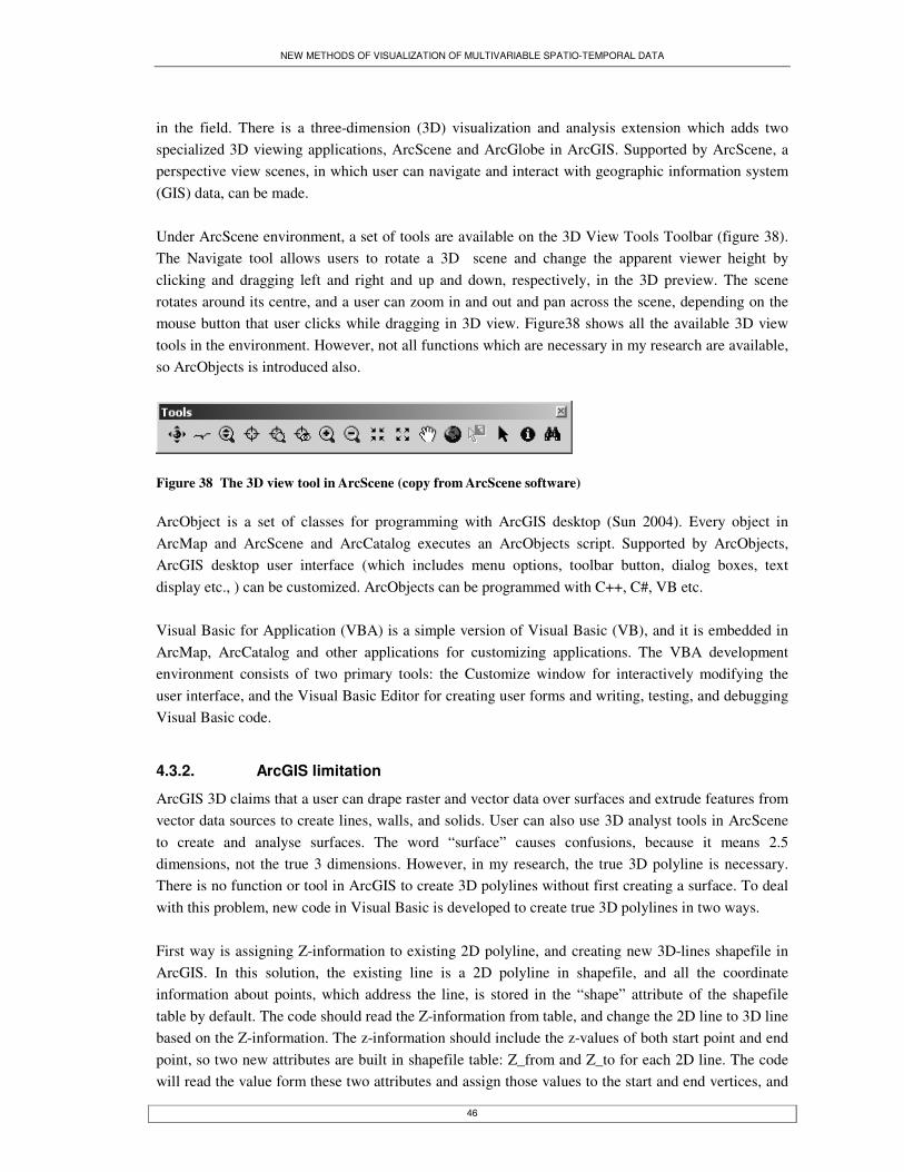
NEW METHODS OF VISUALIZATION OF MULTIVARIABLE SPATIO-TEMPORAL DATA
46
in the field. There is a three-dimension (3D) visualization and analysis extension which adds two specialized 3D viewing applications, ArcScene and ArcGlobe in ArcGIS. Supported by ArcScene, a perspective view scenes, in which user can navigate and interact with geographic information system (GIS) data, can be made. Under ArcScene environment, a set of tools are available on the 3D View Tools Toolbar (figure 38). The Navigate tool allows users to rotate a 3D scene and change the apparent viewer height by clicking and dragging left and right and up and down, respectively, in the 3D preview. The scene rotates around its centre, and a user can zoom in and out and pan across the scene, depending on the mouse button that user clicks while dragging in 3D view. Figure38 shows all the available 3D view tools in the environment. However, not all functions which are necessary in my research are available, so ArcObjects is introduced also.
Figure 38 The 3D view tool in ArcScene (copy from ArcScene software) ArcObject is a set of classes for programming with ArcGIS desktop (Sun 2004). Every object in ArcMap and ArcScene and ArcCatalog executes an ArcObjects script. Supported by ArcObjects, ArcGIS desktop user interface (which includes menu options, toolbar button, dialog boxes, text display etc., ) can be customized. ArcObjects can be programmed with C++, C#, VB etc. Visual Basic for Application (VBA) is a simple version of Visual Basic (VB), and it is embedded in ArcMap, ArcCatalog and other applications for customizing applications. The VBA development environment consists of two primary tools: the Customize window for interactively modifying the user interface, and the Visual Basic Editor for creating user forms and writing, testing, and debugging Visual Basic code.
4.3.2. ArcGIS limitation
ArcGIS 3D claims that a user can drape raster and vector data over surfaces and extrude features from vector data sources to create lines, walls, and solids. User can also use 3D analyst tools in ArcScene to create and analyse surfaces. The word “surface” causes confusions, because it means 2.5 dimensions, not the true 3 dimensions. However, in my research, the true 3D polyline is necessary. There is no function or tool in ArcGIS to create 3D polylines without first creating a surface. To deal with this problem, new code in Visual Basic is developed to create true 3D polylines in two ways. First way is assigning Z-information to existing 2D polyline, and creating new 3D-lines shapefile in ArcGIS. In this solution, the existing line is a 2D polyline in shapefile, and all the coordinate information about points, which address the line, is stored in the “shape” attribute of the shapefile table by default. The code should read the Z-information from table, and change the 2D line to 3D line based on the Z-information. The z-information should include the z-values of both start point and end point, so two new attributes are built in shapefile table: Z_from and Z_to for each 2D line. The code will read the value form these two attributes and assign those values to the start and end vertices, and

NEW METHODS OF VISUALIZATION OF MULTIVARIABLE SPATIO-TEMPORAL DATA
47
then linearly interpolating Z values for all vertices in between. Accordingly, Z values will be added to the “shape” attribute and the true 3D is created and the 3D view can be showed in ArcScene. However, due to the linear interpolation, it is impossible to address exact Z value to each vertex independently. The second part will solve this problem. This solution is necessary because it is good in transforming existing 2D lines to 3D lines without reading the original coordinate information. The second way is directly reading coordinates of 3D points (x, y, z) from table. These vertex points are grouped for 3D polylines by one indicator which is an attribute in a table. Then a new shapefile is created with 3D polylines according the vertices. To achieve this function, the following steps are followed:
1. Create a shapefile feature class; 2. Create a Z-aware polyline object; 3. Create a Point object, read x, y, z from your table, and assign the coordinates to the point; 4. Add the point to the polyline; 5. Repeat steps 3 and 4 until the polyline is completed; 6. Create a new feature, and assign the polyline object to the feature; 7. Add the new feature to the feature class; 8. Repeat steps 2 - 7 until all polylines are completed; 9. Add the shapefile to ArcScene.
The second way is good at creating any shape of 3D polylines with coordinate of vertices, and these coordinate of vertices are useful in my research because these vertices define the state of the object (in Multivariable-Time-Cube). Supported by this tool, any state of object can be addressed in cube. Furthermore all the data can be read from table, which can be defined by the user.
4.4. Realize the PCP-Time-Cube
The concept of PCP-Time-Cube is introduced in chapter 3. In PCP-Time-Cube, X-axis represents different variables, Y-axis represents the range of the value of the object in different variables and Z-axis represents the time. There are two key planes in PCP-Time-Cube: T-PCP plane that identifies a PCP graphic at certain time and V-time plane that identifies a variable with time. An object in PCP-Time-Cube is a surface. From a data aspect, three variables which indicate the economic factor are selected from Provstate table in this case study. They are trade-coefficient, food-coefficient and transport-coefficient which are ratios between the increase/decrease 2003 year and last year per month. User can chose any of these attributes as visualization variables. To investigate the effect of the number of SARS patients in relation to the economic factors, the number of SARS patients and dead patients are chosen also as the other visualization variables. The time scale is per month, and the duration is 12 month from January 2003 to December 2003.

NEW METHODS OF VISUALIZATION OF MULTIVARIABLE SPATIO-TEMPORAL DATA
48
4.4.1. Realization of PCP-Time-Cube with SARS case
4.4.1.1. PCP-Time-Cube reference
To realize the PCP-Time-Cube in ArcScene in this case study conveniently, the X-axis is used to address time, and 12 months in 2003 are evenly assigned on the X-axis. The Y-axis is used to address the five variables, which are introduced in the last paragraph. The height (Z-axis) indicates the different value scope for different variables. in the model (chapter 3), the Z-axis indicates time, and the surface of attribute values is almost a vertical one on which changes in value are shown as far or close to the viewer. So using Z-axis here to indicate values has the advantage of low and high vertex on an undulation surface that characterizes an object. It gives more sense about the changes of the values than the other representation. Based on this design, cube reference is realized in ArcScene by creating edges of the cube only, because this will allow other objects inside the cube (surfaces and polylines) to be visible. Furthermore, 12 T-PCP planes and 5 V-time planes are created also as reference to identify different time and variables.
4.4.1.2. Re-calculate the value to cube height
Because different variables have different values ranges, and the height of the cube is fixed, the values for different variables should be re-calculated to adapt to the height of cube. Furthermore, if several valued of variables have the same units, and a relationship between these variables is expected, these several variables can be re-calculated with the same function based on the value range of these variables. In this case study, the five variables have different range of values, so they should be re-calculated individually based on their maximum and minimum value. The function is:
)()(
MinxMinMax
h −×−
Where h is the height of cube; the Min and the Max are the maximum and minimum values of the variable, and the x is the original value.
4.4.1.3. Overview
After all the values are normalized to the height of cube, based on the reference which is defined before, the surfaces are created. Figure 39 shows an overview of PCP-Time-Cube and the surface is the data of Hainan province in China and Figure 40 shows the framework of the surface. The purple lines indicate variable changes over time, and they are called V-Hainan-time lines which are the intersections of surface with V-time plane. The green lines indicate states of Hainan province at different months, and they are called T-Hainan-variable lines which are the intersections of surface with T-PCP plane. The intersection points of V-Hainan-time lines and T-Hainan-variable lines are the vertexes of surface which correspond to a certain value of the variable of the object at a certain time. In fact, the variable is the V-time plane on which the point is, and the time is the Time-PCP plane on which the point is. For example, in figure 39, the red vertex point is on the V3-time plane and t1-PCP plane, and it is the intersection of t1-Hainan-time line and V3-Hainan-variable line. The height of this point indicates the transport-coefficient of Hainan province at December 2003. The V-Hainan-time lines, T-Hainan-variable lines and the vertexes form the framework of the Hainan surface. As showed
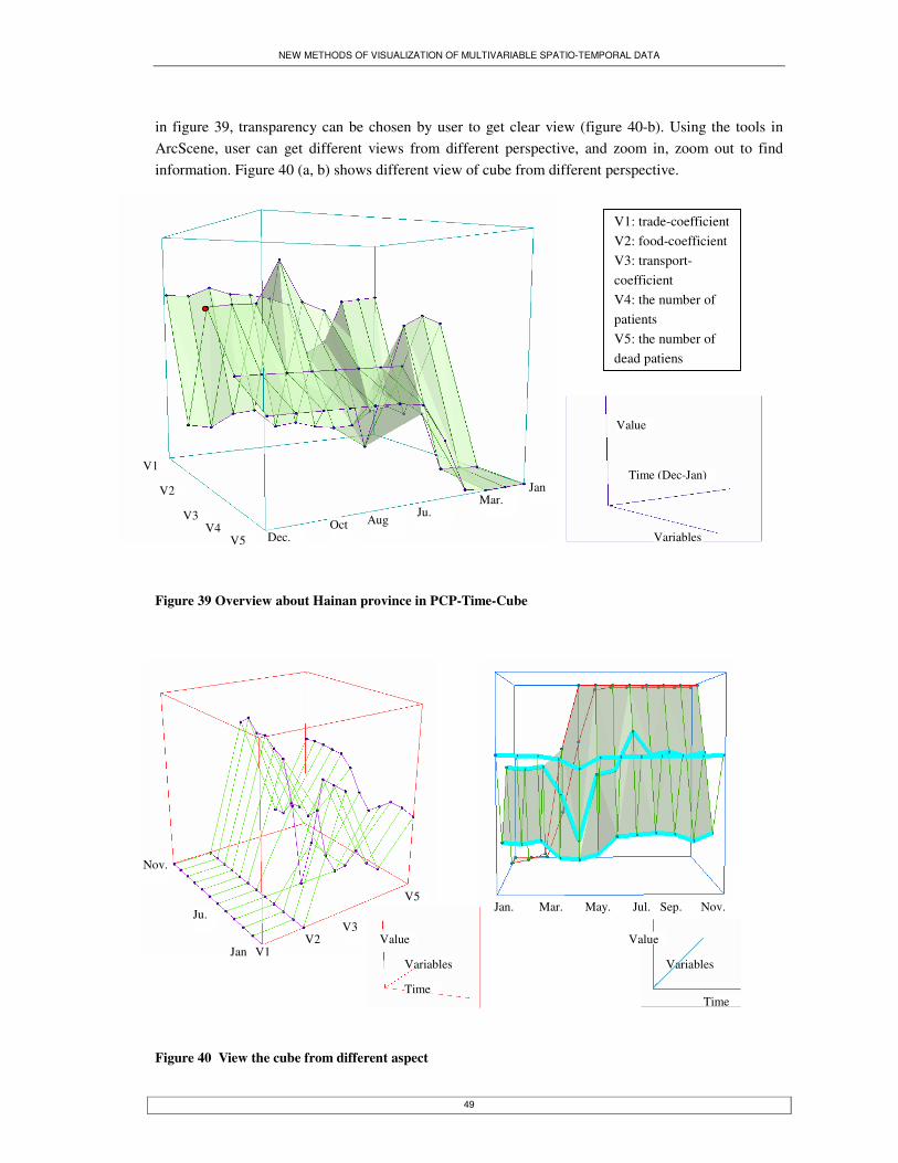
NEW METHODS OF VISUALIZATION OF MULTIVARIABLE SPATIO-TEMPORAL DATA
49
in figure 39, transparency can be chosen by user to get clear view (figure 40-b). Using the tools in ArcScene, user can get different views from different perspective, and zoom in, zoom out to find information. Figure 40 (a, b) shows different view of cube from different perspective. Figure 39 Overview about Hainan province in PCP-Time-Cube Figure 40 View the cube from different aspect
Jan. Mar. May. Jul. Sep. Nov. Dec.
Value
Time
Variables Variables
Time
Value V1
V2 V3
V5
Jan
Ju.
Nov.
Time (Dec-Jan) Jan
Mar. Ju.
Dec. Oct Aug
Value
Variables
V1
V2
V3 V4
V5
V1: trade-coefficient V2: food-coefficient V3: transport-coefficient V4: the number of patients V5: the number of dead patiens

NEW METHODS OF VISUALIZATION OF MULTIVARIABLE SPATIO-TEMPORAL DATA
50
Provinces have different surfaces in PCP-Time-Cube (See figure 41). By viewing the surface from various perspectives, different information can be obtained. For example, figure 42 shows a view from the top of the cube. Colours indicate the surfaces of the provinces. The right part of figure 42 is a legend of the graphic. From this graphic it is easy to see which province has the highest value of a variable at a time. For example, along the time line of the third variable: transport-coefficient, the highest values belong to, from January to December in turn: Chongqing province, Guangdong province, Chongqing province and Hainan province. In the same way, a graphic, viewed from the bottom, will provide the information about lowest value. Figure 41 Overview of PCP-Time-Cube about three provinces
Time (Dec-Jan)
Value
Variables
V1 V21
V3 V4
V5
Apr
Feb
Ju.
Aug
Oct
Nov.
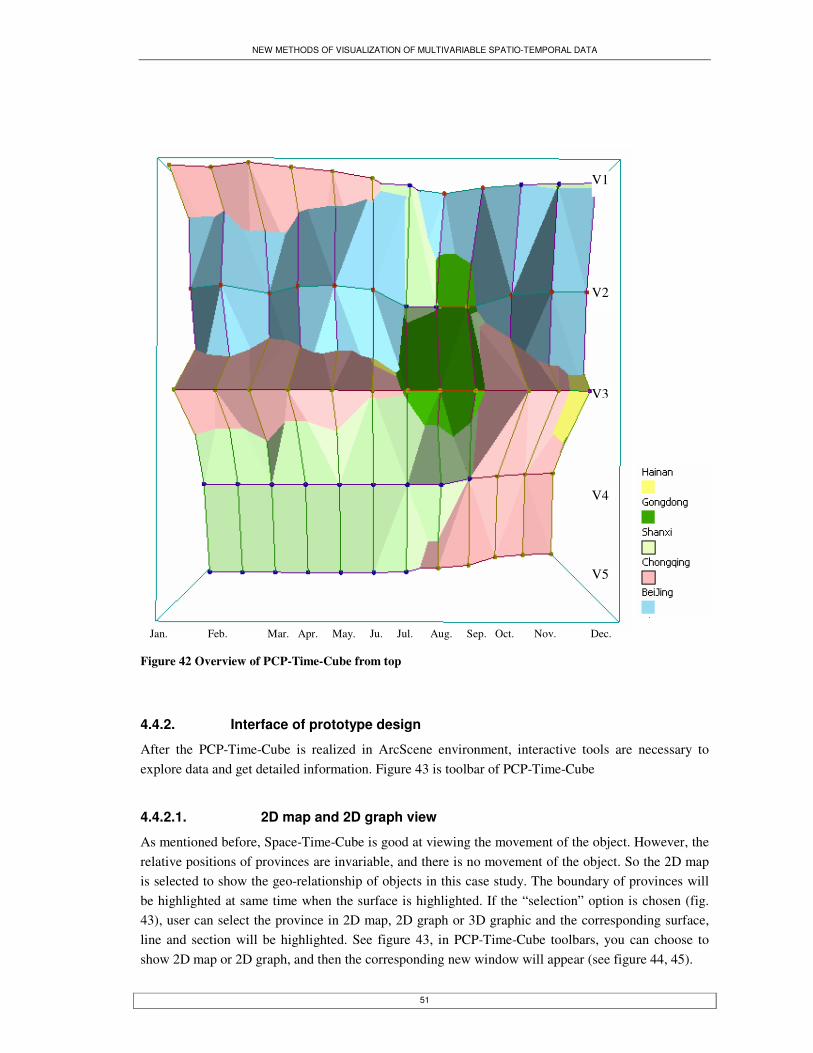
NEW METHODS OF VISUALIZATION OF MULTIVARIABLE SPATIO-TEMPORAL DATA
51
Figure 42 Overview of PCP-Time-Cube from top
4.4.2. Interface of prototype design
After the PCP-Time-Cube is realized in ArcScene environment, interactive tools are necessary to explore data and get detailed information. Figure 43 is toolbar of PCP-Time-Cube
4.4.2.1. 2D map and 2D graph view
As mentioned before, Space-Time-Cube is good at viewing the movement of the object. However, the relative positions of provinces are invariable, and there is no movement of the object. So the 2D map is selected to show the geo-relationship of objects in this case study. The boundary of provinces will be highlighted at same time when the surface is highlighted. If the “selection” option is chosen (fig. 43), user can select the province in 2D map, 2D graph or 3D graphic and the corresponding surface, line and section will be highlighted. See figure 43, in PCP-Time-Cube toolbars, you can choose to show 2D map or 2D graph, and then the corresponding new window will appear (see figure 44, 45).
Jan. Feb. Mar. Apr. May. Ju. Jul. Aug. Sep. Oct. Nov. Dec.
V1
V2
V3
V4
V5

NEW METHODS OF VISUALIZATION OF MULTIVARIABLE SPATIO-TEMPORAL DATA
52
The 2D graph view (see figure 45) is used to show the T-PCP planes and V-time planes which are extracted from the PCP-Time-Cube. There are two ways to open this window. One is selecting “show 2D graph” in PCP-Time-Cube, and selecting the graphic in the new window. The other one is double clicking the point which identifies the month or variables in PCP-Time-Cube 3D view. Figure 43 PCP-Time-Cube toolbars Figure 44 2D map view in PCP-Time-Cube Figure 45 An example of 2D graph view about trade-coefficient-time plane
Jan. Feb. Mar. Apr. May. Ju. Jul. Aug. Sep. Oct. Nov. Dec.

NEW METHODS OF VISUALIZATION OF MULTIVARIABLE SPATIO-TEMPORAL DATA
53
4.4.2.2. 3D view
PCP-Time-Cube is in the 3D view. All the tools that are supplied by ArcScene can help user to get different view of the cube: navigate, fly, zoom in/out, centre on target etc. In this way, the user can get different information about the data
4.4.2.3. Identify result window and selection tools
The identify result window is used to give the detailed information about the vertex point, T-Object-variable line, T-object-time line or surface which is selected by the identified tools (see figure 47). Only if the identify button is active and select any point, line or surface, the identify result window will show the detail value about attributes of each object. The selection tools are used to select surface, lines and point in 3D graphic, 2D map or 2D graph. Figure 46 Identify result window
4.4.3. Questions about multivariable spatio-temporal data in PCP-Time-Cube
After the visualization prototype is designed in this case study, the four components of multivariable spatio-temporal data mentioned in chapter two, will be identified at first. In this case study, the objects are provinces which are visualized as different surfaces. Temporal variable, i.e. twelve months in 2003, are addressed on X-axis, and five variables are on Y-axis. Based on this reference and the interactive tools, the typical questions to the Space-Time-Cube will be addressed in this section one by one.
4.4.3.1. What����where+when+how
As mentioned before, the provinces are identified by different surfaces. All information about the province should be on the surface. User can choose the surface or the framework of the surface: time lines, variable lines and vertex points to view the changes of variables of provinces with time. For example, in figure 47, the yellow surface identifies Hainan province, five time-lines (highlight lines in fig.47) for different variables of Hainan province are selected in PCP-Time-Cube, the boundary of Hainan province is highlighted also in 2D maps that shows “where”. The overview about “when”+ “how” can be viewed in PCP-Time-Cube. When the identify tool is active, the corresponding value about “when” and “how” can be obtained in identify result window by clicking the points or lines.
How Where
What
When

NEW METHODS OF VISUALIZATION OF MULTIVARIABLE SPATIO-TEMPORAL DATA
54
Furthermore, the user can choose whether other surfaces or frameworks are shown, and relationship between the selected provinces with other provinces can be viewed. Figure 47 Hainan province is characterized in PCP-Time-Cube, 2D map and identify window.
Time
Value
V1
V2
V3
V4
V5
Jan
Apr
Feb
Ju.
Aug
Oct
Nov.
Variables

NEW METHODS OF VISUALIZATION OF MULTIVARIABLE SPATIO-TEMPORAL DATA
55
4.4.3.2. When����where+what+how
The twelve time-PCP planes in PCP-Time-Cube address this question. Clicking the point, which identifies one month on X-axis or selecting the T-PCP plane in 2D graph window, the corresponding PCP plane of this month will be shown in 2D graph view. The left T1-PCP in figure 48 shows the state of provinces at January 2003. It should be mentioned that if any province is selected, the corresponding line about the province will be highlighted also in 2D graph, and if the line is selected in 2D graph, the surface of the same province will be highlighted also. In the T-PCP plane, the value of all provinces at T1 time can be addressed. To get further information about “where”, a user can select a line in 2D graph, and the boundary of the selected province will be highlighted in 2D map (see right map in figure 48). Figure 48 Chongqin province is highlighted in January-PCP plane and 2D map
4.4.3.3. Where����when+what+how
As mentioned before, in this prototype, the 2D map is used to address the “where”. To answer this question, a province or several provinces can be selected in 2D map. The corresponding surfaces will be highlighted in PCP-Time-Cube, and the state or relationship among multivariable of province(s) can be viewed and further studied. For example, selecting provinces which are near Beijing (figure 49), results in the corresponding surfaces shown in PCP-Time-Cube. They all have relative high value on the number of patients and the economic situations are relatively bad in April, May and June. This indicates that Beijing may be the centre of SARS, i.e. the key location for spreading SARS. Furthermore, the irregularities can also be found in PCP-Time-Cube. For example, in figure 50, the highlight of time lines belong to Hainan province, and the 2D map shows that it is far away from Beijing. However, the transport-coefficient is affected badly, which can be viewed in PCP-Time-Cube of figure 50. This irregularity is because that the Hainan is a tourist city, and May is the best travel season in this province. Because of SARS, almost all travel projects are stopped, and therefore the decrease of transport is sharp.
V5 V4 V3 V2 V1
How Where
What
When
How Where
What
When

NEW METHODS OF VISUALIZATION OF MULTIVARIABLE SPATIO-TEMPORAL DATA
56
Figure 49 Identify provinces which near by Beijing Figure 50 Hainan province in PCP-Time-Cube and 2D map
4.4.3.4. How ����when+ what+ where
In PCP-Time-Cube, Variable-time-planes identify different variables. User can click a variable point on Y-axis, and the corresponding variable plane will be shown in 2D graph. For example, figure 51 shows the information about trade-coefficient of some provinces with time. The vertical black lines indicate different months and the colour lines indicate the value changes of trade-coefficient of different provinces. Users can also find any interested vertex point in PCP-Time-Cube, as figure 52.
How Where
What
When
Time
Value
Variables
Variables Time
Value
Jan. Mar. May. Jul. Sep. Nov.
V1
V2
V3
V4
V5

NEW METHODS OF VISUALIZATION OF MULTIVARIABLE SPATIO-TEMPORAL DATA
57
The left figure shows the view from left side of the cube, and five variables are shown together. If an interesting value is discovered, a click at the 2D graph or 3D PCP-Time-Cube, will identify the object. In the right graphic of figure 52, all the frameworks about the identified province will be highlighted. At the same time, the boundary of the identified province is highlighted also in 2D map and the relationship between the variables can be viewed also. For example, in figure 53, the province with higher values on the trade-coefficient, food-coefficient and transport-coefficient have lower values for the number of patients. It indicates that the affection of SARS is obvious. Figure 51 Trade-time plane for different provinces extracted from PCP-Time-Cube Figure 52 A province of Shandong is highlighted
Jan. Feb. Mar. Apr. May. Ju. Jul. Aug. Sep. Oct. Nov. Dec.
V5 V4 V3 V2 V1 V5 V4 V3 V2 V1
Variables Time
Valu

NEW METHODS OF VISUALIZATION OF MULTIVARIABLE SPATIO-TEMPORAL DATA
58
Figure 53 An overview of 4 provinces
4.4.4. Summary of PCP-Time-Cube
PCP-Time-Cube combines all the information about multivariables of an object with time in one cube. So both the value about individual variable and the relationships between variables of the objects can be viewed together. In PCP-Time-Cube, the vertex points identify “what+when+how”, the time-lines identify “what+how”, the variable lines identify “what+when”, the time-PCP planes identify “what”, the V-time planes identify “how” and the surfaces identify “what”. All these points, lines and planes form PCP-Time-Cube that provides an overview of all multivariables of objects with time. Table 7 shows how the components of multivariable-temporal data are addressed in PCP-Time-Cube. However, to get geo-information, the PCP-Time-Cube should be linked to 2D map in this case by “what” component. The usability evaluation will be further discussed in the chapter five.
Variables
Time
Value
V1 V2
V3 V4
V5
Apr
Feb
Ju.
Aug
Oct
Nov.

NEW METHODS OF VISUALIZATION OF MULTIVARIABLE SPATIO-TEMPORAL DATA
59
Component Is visualized in PCP-Time-Cube What surface When T-PCP plane Where V-time plane What+when surface + T-PCP plane =T-object-variable line What+how surface +V-time plane=V-object-time line What+when+how T-object-variable line+ V-object-time line= vertex point Table 7 The multivariable spatio-temporal components in PCP-Time-Cube
4.5. Realize the Multivariable-Time-Cube
In Multivariable-Time-Cube, two variables, two user-defined variables replace the geo-X and geo-Y coordinates of Space-Time-Cube. Accordingly, the geo-space is replaced also by a variable space. While in Space-Time-Cube, the trajectory of an object indicates the change of geo-location; in the Multivariable-Time-Cube it indicate the value change. However, only two variables can be represented in one cube. Two solutions are proposed in this research to this problem. One is to introduce more Multivariable-Time-Cubes, and the other is the option for a user to define any attributes on X-axis and Y-axis. The later method is realized in this research. In this case study, the data about twenty SARS patients is used. It includes the movement of patients and the state of patients at different time, and the duration is 80 days from 20 April to 30 June 2003. As mentioned before, the Space-Time-Cube is used to show the movement of the patients and the multivariables which include the body temperature, infection, resistance, environment temperature etc. in Multivariable-Time-cube.
4.5.1. Realization of Multivariable-Time-Cube with SARS case study
4.5.1.1. Reference and re-calculated the valued with the cube size
For time variable, to maintain the synchronism of different cubes, the Z-axis of each cube is defined with the same scale of time by days, and the duration is 80 days from 20 April, when the SARS Office of Ministry of Health People’s Republic of China began to publicize the data, to 30 June when no new patient appeared. As with the PCP-Time-Cube, the value should be recalculated to adapt to the size of the cube. In Space-Time-Cube, the scope of China is limited in cube size, all the distance between city and scope of provinces are at the same scale. For Multivariable-Time-Cube, the size is the same as the Space-Time-Cube, and all the value ranges of variables should be re-calculated to adapt to the cube size by the function mentioned before. The reference is showed in figure 54.

NEW METHODS OF VISUALIZATION OF MULTIVARIABLE SPATIO-TEMPORAL DATA
60
Figure 54 Reference of Multivariable-Time-Cube
4.5.2. Prototype interface
After the Multivariable-Time-Cube is realized in ArcScene environment, interactive tools are necessary to explore data and get detailed information.
4.5.2.1. Toolbar of multivariable-Time-Cube
Figure 55 shows the toolbar of multivariable-Time-Cube. A user can open any table in the database by using the first tool, then the corresponding attributes will automatically be stored on the list of option for cubes. Figure 56 shows the interface after a user opened the table and clicked the “option for cubes” on the toolbar. The Z-axis is defined as time by default, and the X-axis and Y-axis of the first cube are defined as geo-X and geo-Y by default also. So the first cube is basic Space-Time-Cube. For the second cube a user can define any attributes included in the selected table. After each axis is defined, the cube will be created in 3D view. In 3D view, based on the ArcScene environment, the view tools, which are mentioned in PCP-Time-Cube, are available also. Figure 55 Toolbar of Multivariable-Time-Cube
Variable1
Time
X
Time
Variable2 Y

NEW METHODS OF VISUALIZATION OF MULTIVARIABLE SPATIO-TEMPORAL DATA
61
Figure 56 Parameters option for cubes
4.5.2.2. Synchronism link and identify selection
After the cube is created, a user can choose synchronism link by clicking “synchronism reference” on the toolbar. Then the window will open (see figure 57-a). All the potential value of the attributes is available when the attribute option is selected. In this figure, “what” component is selected, and the patient’s id can be chosen from 1 to 20. Figure 58 shows the result in 3D view after “what” is selected and patient 1 is identified. The X-axis is defined as SARS situation, and Y-axis is defined as body-temperature (BT). Figure 57-b shows identify selection window used to identify “where” or “how”. As mentioned before, “where” and “how” cannot be a synchronism link, so this window help user to identify a location or a exact value of selected variable in 3D and 2D view ( the identified section will be highlighted). In fact, this function is similar with the “what+when” selection in synchronism reference define window, because the identify results of “where” or “how” are section of trajectory in both Space-Time-Cube and Multivariable-Time-Cube about “what+when” and “what+when” is use to transport link information to other cube. Figure 57 Synchronism reference definition window and identify section window
(a) (b)

NEW METHODS OF VISUALIZATION OF MULTIVARIABLE SPATIO-TEMPORAL DATA
62
Figure 58 Patient whose id is “1” identified in Multivariable-Time-Cube
4.5.2.3. 2D map and 2D graph
As in PCP-Time-Cube, 2D map is used to supply geo-information. After the 2D map button is clicked, the 2D map will be shown. The 2D map is mainly used to select the location. The trajectory, which passes through the selected location, will be highlighted. As mentioned before, the projections of trajectories on the bottom, back face and side face in Multivariable-Time-Cube are all meaningful. 2D graph view is used to show the information about the projection of trajectory. In 2D graph window, selecting the V1-V2, V1-t or V2-t, the corresponding graphic will be shown. The figure 59 shows V1-t graph and is this case the V1 is SARS variable.
BT
Time
X
Time
SARS Y

NEW METHODS OF VISUALIZATION OF MULTIVARIABLE SPATIO-TEMPORAL DATA
63
Figure 59 SARS variable change with time graphic
4.5.2.4. Identify result window and selection tools
Same as is PCP-Time-Cube, the identify result window will provide detailed information depending on the user selection and the existing data if the identify tool is active and the selection tools help user to select trajectory or different projection in 3D view and 2D view. And the selected object will be highlighted.
4.5.2.5. Option in Space-Time-Cube
As mentioned before, to visualize more variables, one method for user is to define the X and Y axis. In fact, the colour and size of trajectory can be variables also. In figure 60, the red lines show the duration in which a patient has fever. The blue lines indicate the non-fever duration. In figure 61, the red line shows the highest infection. It means that the person was infected with SARS, but he or she did not stay in hospital. A user can choose different variables and different classification methods to explore the information by himself.
H U Ce Cu D
T
SARS

NEW METHODS OF VISUALIZATION OF MULTIVARIABLE SPATIO-TEMPORAL DATA
64
Figure 60 Fever state is represent as red and un-fever is represent as blue Figure 61 Danger trip is represent as red line.
Time
X Y
Time
X Y

NEW METHODS OF VISUALIZATION OF MULTIVARIABLE SPATIO-TEMPORAL DATA
65
4.5.3. The questions about Multivariable spatio-temporal data in Multivariable-Time-Cube
In this case study, the objects are patients which are visualized as trajectories in two cubes. Temporal variable, 80 days from 10 April to 30 June 2003 is addressed on Z-axis, the first cube is Space-Time-Cube, and X-axis and Y-axis of Multivariable-Time-Cube can be defined by a user. This section discussed how the simplest four questions of multivariable spatio-temporal data are dealt with in Multivariable-Time-Cube.
4.5.3.1. When ���� how + what+ where
This question can be answered by identifying the temporal variable. The method defines “when” component as synchronism reference, and enables selection of a day in the synchronism reference window, or a click on the Z-axis at any cube. Then the corresponding T-planes appear in two cubes (see figure 62).The geo-information of objects can be viewed by intersection of the trajectories with the T-plane. The values of the variables can be got from the Multivariable-Time-Cube. However, only the values of the variables which are defined on X and Y axes can be gotten. A user can define different variables on X and Y axes to get the other values. Figure 62 A time plane identify a time in Multivariable-Time-Cube
26 May 2003
Time
X Y
Time
Infective SARS
How Where
What
When

NEW METHODS OF VISUALIZATION OF MULTIVARIABLE SPATIO-TEMPORAL DATA
66
4.5.3.2. What ����when+ how + where
A patient should be first identified to answer this question. Clicking a trajectory one cube, the two trajectories, which identify the same patient in both cubes, will be highlighted at the same time. The other way is to define “what” component as synchronism reference and selected id of the patient. The “when+ how” can be derived in Multivariable-Time-Cube or 2D graphs of projections, and the “when+ where” can be answered in Space-Time-Cube. In figure 63, the “patient 1” is highlighted in two cubes and on 2D graph. Figure 63 A patient is highlighted in Multivariable-Time-Cube and 2D graph. In 2D graph (V1-time), the patient dead because the body-temperature become 0 at 25/5/2004
B-T 37oC 0oC
25/5/2004
How Where
What
When
SARS
B-T Time
X
Y
Time

NEW METHODS OF VISUALIZATION OF MULTIVARIABLE SPATIO-TEMPORAL DATA
67
4.5.3.3. Where ����when+ what+ how
As mentioned before, a 2D map is used to select a location and the synchronism reference can also be used by selecting the name of a province. The trajectory sections, which are inside the area, will be highlighted in Space-Time-Cube. Furthermore, based on the information about the patient and time, the corresponding information will be highlighted in Multivariable-Time-Cube.
4.5.3.4. How ����when+ what+ where
This question can be answered by using optional colors in Space-Time-Cube. See the example in 4.5.3.6. The second method is to select “how” component in identify selection window. After the variable is selected, the corresponding potential values of this selected variable will be shown in the list. Select the value and the trajectory sections which is the value will be highlighted, and the corresponding information about “when+what” can be viewed in Multivariable-Time-Cube and the corresponding information about “when+what+where” can be derived in Space-Time-Cube.
4.5.4. Summary of Multivariable-Time-Cube
In Multivariable-Time-Cube, the object is represented by polyline, which indicates the value changes of the selected variables. Table 8 shows how the four components of multivariable spatio-temporal data are addressed in Space-Time-Cube and Multivariable-Time-Cube. Component In Space-Time-Cube In Multivariable-Time-Cube What Trajectory Trajectory When T-plane T-plane (V1-V2 plane) Where Vertical lines How Vertical lines How+when V-time plane What+when Intersection of trajectory
and T-plane Intersection of trajectory and T-plane
Where+how When+where Intersection of time plane
and the vertical line
What+how Intersection of time plane and the vertical line
What+when+where Point What+when+how Point Table 8 Four components of MSTD and addressed in Space-Time-Cube and Multivariable-Time-Cube
How Where
What
When
How Where
What
When

NEW METHODS OF VISUALIZATION OF MULTIVARIABLE SPATIO-TEMPORAL DATA
68
In this case study, two aspects are different from the PCP-Time-Cube. The first one is using Space-Time-Cube to represent geo-information because 2D map is difficult to show spatio-temporal data. In this case study, the Space-Time-Cube is linked to Multivariable-Time-Cube to represent Multivariable spatio-temporal data. The second one is using synchronism link to link two cubes. Based on the prototype, the questions about multivariable spatio-temporal data can be addressed. The evaluation of the two prototypes will be discussed in the next chapter.
4.6. Summary
In this chapter, PCP-Time-Cube and Multivariable-Time-Cube are realized as prototypes using SARS data. The interactive environments for two models are designed and developed. In these two prototypes, 2D map and Space-Time-Cube are used individually to provide geo-information. However, whether the model can be understood and multivariable spatio-temporal data are represented properly is another important part in this research? Therefore, the usability evaluation will be discussed in next chapter.

NEW METHODS OF VISUALIZATION OF MULTIVARIABLE SPATIO-TEMPORAL DATA
69
5. Usability evaluation of prototypes
5.1. Introduction
Based on models which are designed in chapter 3, two prototypes PCP-Time-Cube and the Multivariable-Time-Cube are designed and realized in chapter 4 in ArcScene using SARS data. However, a usability evaluation is necessary because the objective of this research is a usable visualization solution. In recent years usability of GIS products and specifically geo-visualization tools has received considerable attention and it is increasingly the focus of a number of research activities in the GIS-science field (Koua 2005). Increasing research interest in the usability of geo-information systems has been demonstrated by Mac Eachren (2001), Tobon (2003), Fuhrmann (2004) and Koua (2004). ISO9241-11 defines usability as the extent to which a product can be used by specified users to achieve specified goals with effectiveness, efficiency and satisfaction in a specified context of use (Bevan 1994). In this evaluation, 9 persons who are in different professional fields are grouped to three groups to evaluate the PCP-Time-Cube and Multivariable-Time-Cube. The evaluation results are summarised and analysed to get the usability information.
5.2. Evaluation objective
As mentioned before, usability evaluation is necessary because the objective of this research is a usable visualization solution, and evaluating the usability of prototypes is addressed in one of the research questions. ISO9241-11 defines usability at three levels - effectiveness level, efficiency level and the degree of satisfaction with which users achieve their tasks with the test object in question. ISO9241-11 defines effectiveness, efficiency and satisfaction as follows:
• Effectiveness: The accuracy and completeness with which users achieve specified goals. • Efficiency: The resources expended in relation to the accuracy and completeness with which
users achieve goals. • Satisfaction: The comfort and acceptability of use.
Starting from the three levels of usability, the more detail questions in this evaluation were; 1. Are the two models user easily understood by users? 2. Which model is good at answering which multivariable spatio-temporal questions? 3. Which geo-visualization functions are useful for users to explore multivariable spatio-
temporal data in PCP-Time-Cube and Multivariable-Time-Cube? 4. Which prototype gives more sense about multivariable spatio-temporal data: the one link with
Space-Time-Cube or 2D map?

NEW METHODS OF VISUALIZATION OF MULTIVARIABLE SPATIO-TEMPORAL DATA
70
5.3. Evaluation
Although there are many evaluation methods: Card sorting (Nielsen, 1993), Verbal protocol analysis (VPA) (Ericsson, 1993), Focus group (Morgan, 1998) and questionnaire etc., the focus group and questionnaire method have been selected and combined in this research to evaluate the prototypes, because focus group is even faster than VPA and generates a similarly large amount of data. In general, focus groups allow users to share their experience with an application and develop hypothetical situations/ideas in a quick and efficient manner (Anthony, 2005). A questionnaire follows the focus group to gather subjective opinions about the usability of the prototypes. Then better justify the choice, e.g. by emphasizing that the models and visualizations are rather complex. A good initial impression of user reactions can be effectively obtained via the focus group and questionnaire methods. Results of the focus group and questionnaire could be used to improve models/prototype, which could then be subjected to detailed evaluation with many potential users. However, because of time constraints this detailed evaluation cannot be done within the current research.
5.3.1. Focus groups evaluation
Focus groups (Morgan 1998) is an evaluation method that solicits ideas and feedback through a group discussion (Robinson 2005), it is a seemingly informal technique that can be used to evaluate the user requirements and feelings about a prototype (Nielsen 1993). It is actually a quick way of evaluating a prototype (Faulkner 2000). Focus groups belong to the branch of qualitative research methods (Morgan 1998). Therefore data elicited from a focus group session can be used to qualitatively discuss the advantages and disadvantages of prototypes, and the users’ attitude towards the interface of a prototype or towards the test object in the prototype: in this case visualization solutions for multivariable spatio-temporal data. Focus groups work optimally when the group members have an interest in the subject of the research (Morgan 1998). Such members are usually a group of six to nine (Nielsen 1993) who can openly discuss the issues put forward by the moderator about the prototype. One criterion to predict a permissive environment to all members for full participation in the discussion is equality of status (Monmonier 1994), especially, of background regarding the topic of discussion.
5.3.2. Questionnaire evaluation
Questionnaires are old and established methods, which do not directly study the object of evaluation (here the prototypes), but rather the user’s opinions about the object (Tšoene, 2003). As a consequence, in this work, after the prototypes were applied it was supplemented by a questionnaire wherein questions about ‘subjective’ issues were put forward to the user pertaining to the usability of the visualization techniques in the prototypes. The issues addressed in the questionnaire (Appendix A) were the usability merits recommended by ISO 9241-11 (1998) as outlined in chapter 2; effectiveness, efficiency, and the degree of satisfaction with which the test subjects achieved their test tasks.
5.3.3. Evaluation plan and overview
The evaluation plan was divided into five parts. � Evaluator gives an opening speech for less than 5 minutes to welcome the persons who take
part in this evaluation and introduce the objective of this evaluation.
NEW METHODS OF VISUALIZATION OF MULTIVARIABLE SPATIO-TEMPORAL DATA
71
� Evaluator gives a presentation for 10 minutes to introduce the prototypes and basic concepts about multivariable spatio-temporal data.
� Evaluator gives a demo with explanation about PCP-Time-Cube and Multivariable-Time-Cube for 5 minutes.
� Participants discuss and carry out the task with prototypes and evaluator record the time � Participants discuss and filling-out a questionnaire about their feeling about the prototypes. � Participants discuss and give suggestions.
5.3.4. Evaluation members
The members are grouped into three groups based on their speciality: the first group consisted of three ITC students who in Geo-visualization. They have experiences and knowledge about visualization solutions. The second group consisted of three ITC students who in different programs: Nature Resources Management, Urban Planning and Land Administration and Environmental Management. They have some work experiences in their own fields but have not much visualization experience. The last group consisted of three experts who are engage in meteorology, geology and environmental study. The reason for this grouping is that they have different experience level regarding the multivariable spatio-temporal data visualizations. The members of the first group know basic concepts about multivariable spatio-temporal data, and the existing visualization solutions, but they have little chance to deal with application, so they analysed the prototype on conceptual level. The members of the second group deal with a lot of data in their fields but have less experience in visualization. They are blank users who evaluate the degree of intelligibility based on their own experience. The members of the last group have experiences in both data and visualization solutions. They compare the models with more convention representations, to which they are used, and evaluate the usability of the prototypes developed in this research by filling in the questionnaire.
5.3.5. Tasks design
Based on the evaluation objective, questions are designed to help participants to make sense of the models. It helps them to fill in the questionnaire and their answers will be more meaningful. The time needed to which they answer the following questions is used as measure of efficiency. Tasks are designed at three levels. The first level is an overall level to test the understanding of graphics and ability to make different views. The second level is filtering information from the 3D views and 2D graphics and understanding relationship between them. The third level has detailed questions about the four components: when, where, what and how to test the effectiveness of the prototypes. Although, different data are used in PCP-Time-Cube and Multivariable-Time-Cube, with the tasks designed on the three levels, I try to keep balance between two prototypes. To compare the tasks easily, the tasks are listed in table.

NEW METHODS OF VISUALIZATION OF MULTIVARIABLE SPATIO-TEMPORAL DATA
72
PCP-Time-Cube Multivariable-Time-Cube
How to make a view about Beijing, Hebei and Heilongjiang?
How to make a view, which about two interested attributes
Tasks 1: Overall How to get different views of a cube from different aspects of the cube?
How to get different views of a cube from different aspects of the cube?
How to get the relationship between different variables about Hainan?
How to get the relationship between different variables of patient 1?
How to get the relationship between different provinces about transport-coefficient-time?
How to get the relationship of change between different patients on body-temperature?
Tasks2: Intermediate
How to get the information about the states of provinces at April 2003?
How to get the information about the states of patients on 30 April 2003?
How Which province has the highest value of trade-coefficient? Where is it? When?
When and where is the trip most dangerous for infection?
What What is the value of food-coefficient of Hainan in August 2003? Where is it?
What is the value about SARS situation of the patient-11 at 23 May 2003? Where is he?
When What are the states of provinces in September 2003?
How are certain SARS patients on 25 April 2003, and where are they?
Tasks3: Detailed
Where How is the situation of the province near Beijing?
Who are on the train from Beijing to Shanxi? And what are the in states?
Table 9 Task design in evaluation: The how, what when and where means the simple questions of multivariable spatio-temporal data, which was mentioned before. How ����when+where+what, What����when+where+how, When����what+where+how and Where����when+what+how During tasks fulfilment, the members of each group discuss together and give the solution for questions. The task 1 is simple process of prototype and task 2 ask participant understand the data structure in visualization. These two tasks have not exact answer, so the participants practise on computer and explain it to evaluator and only the time cost is recorded. The task 3 has exact answer, so both the correctness and time cost are recorded.
5.3.6. Evaluation sessions
As mentioned before, the participants are assigned to three groups, and the evaluation sessions are hold per group. Table 10 shows the time and location of the evaluation sessions.
Time Location Group 1 28/01/2005 3:40 pm Room 2061 of ITC Group 2 28/01/2005 5:30 pm Room 2061 of ITC Group 3 29/01/2005 10:30 am Room 2061 of ITC Table 10 The evaluation sessions

NEW METHODS OF VISUALIZATION OF MULTIVARIABLE SPATIO-TEMPORAL DATA
73
Same opening speech was given to the three groups to address the objective of this evaluation: the method used, and the tasks of participants in this evaluation. Then a presentation about the concept of model and environment of prototype and the presentation highlighted the following issues:
• The basic concepts on multivariable spatio-temporal data; • The basic concepts on Space-Time-Cube and PCP; • The basic concepts on PCP-Time-Cube and Multivariable-Time-Cube. It includes the
definitions of V-time plane and T-variable plane projection plane etc.; • The data used in this case study; • The interactive environments of the two prototypes.
Based on the presentation, a demonstration of the case study was given in the interactive environment of PCP-Time-Cube and Multivariable-Time-Cube. Realized interactive tools were explained one by one to show how the tools in both prototypes are used and what can be done supported by the prototypes. Then participant discussed the prototypes to promote the understanding each other and share opinions. Then the participants are asked to perform the tasks. The time, spent on each tasks, and correctness are recorded. Furthermore, a questionnaire has to be filled in by participants. The detailed information about questionnaire is shown in Appendix A. Five grades are defined to standardize the answers:
0~1: very poor 1~2: poor 2~3: fair 3~4: good 4~5: excellent
After questionnaire part, the last part of evaluation is discussions and suggestions. Then the results of discussion are submitted by each group. The summary of results and discussion of the evaluation are discussed in following section.
5.4. Evaluation results
The most important part of a focus group is the discussion of the issues pertaining to the usability of the object under evaluation (Tšoene 2003). During the evaluation, the participants discuss the understanding of prototypes and try to finish tasks. Their discuss results are concluded with the result of questionnaire. Should be mentioned is the results obtain in this evaluation is only initial information about prototypes because only 9 participants in total. So the results will be used to improve the prototypes (will be mentioned in further work). These prototypes will be again tested (but objectively) with a larger sample of users.
5.4.1. Intelligibility and manoeuvrability
In the questionnaire, two questions address the issue of intelligibility of the prototypes. One is the impression of the two prototypes: how much do you understand PCP-Time-Cube and Multivariable-Time-Cube. The other is a detailed table that ask participants to fill value about three usability

NEW METHODS OF VISUALIZATION OF MULTIVARIABLE SPATIO-TEMPORAL DATA
74
measures: effectiveness, efficiency and satisfaction. The consistency of two results of the two questions which address the intelligibility issue, confirm on creditable of results. The impression result for PCP-Time-Cube is 4.5 and for Multivariable-Time-Cube is also 4.5. The more detailed results for intelligibility are shown in Table 11. The columns show some initial information (average results from questionnaires) which given by three groups PCP-Time-Cube Multivariable-Time-Cube Group1 Group2 Group3 Group1 Group2 Group3 Effectiveness 4 4.3 4 4 3.6 4.3 Efficiency 4 4.3 4.6 4 3.6 4.3
Satisfaction 3.6 4.6 4 4.3 4 4.3
Table 11 The results of intelligibility of prototypes The detailed results, which shown in the Table 11, accord to the summary impression, so the results are creditable. The results give the impression that two models are not difficult to understand. However, the values provided by the second group Multivariable-Time-Cube are relatively low. The members explain that trajectories in 3D give less sense when the two variables, which are defined on X and Y axes, are not relevant to each other. However, the expert group thinks that Multivariable-Time-Cube is good for studying the relationship between two variables when the relationship is the objective of study. The question about manoeuvrability of the prototypes is that if they had use their own data in two prototypes and Table 12 shows the results of their opinions. The columns show results (average results from questionnaires) which given by three groups
PCP-Time-Cube Multivariable-Time-Cube Effectiveness 4.6 4.6 4.5 4.3 3.6 4 Efficiency 3.3 4 4 4 4.6 4.5
Satisfaction 3 4.3 4.3 4 4 4.5
Table 12 The results of maneuverability of the prototypes In table 12, effectiveness of PCP-Time-Cube is relative high. The members explained that the PCP-Time-Cube can visualize more variables with time together and it is a powerful integration of data. However, the efficiency and satisfaction is relatively low which can be explained by the fact that 3D graphic in PCP-Time-Cube looks complex, especially, when the number of objects is large. The third group (geo-visualization professional) is interested in Multivariable-Time-Cube. They think Multivariable-Time-Cube is flexible and it is a natural combination of Multivariable-Time-Cube and Space-Time-Cube. They said when a user defines the variables on X and Y axes, it become more clear what to study. From the results, it seems that the PCP-Time-Cube is more effective and Multivariable-Time-Cube is more efficient and satisfying.
5.4.2. Efficiency
The time, used for finishing the tasks, provides further information on the efficiency of the prototypes. The average results are shown in table 13. The detailed tasks are mentioned in section 5.3.3.

NEW METHODS OF VISUALIZATION OF MULTIVARIABLE SPATIO-TEMPORAL DATA
75
Task 1 Task 2 PCP-Time-Cube 3.5 14 20 50 45 Multivariable-Time-Cube 60 11 18 45 Table 13 (unit: seconds) The average time used on task 1 and task 2 by all participants Although different data is used in different prototypes, the tasks designed for the two models are similar to get meaningful results. The blank cell in Table 13 means that the participants cannot answer the questions and the reason will be discussed following below. As mentioned before three levels of the tasks provide different levels of understanding of prototypes. The task 1 and task 2 are overall and intermediate tasks and the objective of these tasks is testing whether the participants understand the 3D graphics and know how to use the interactive tools of prototypes. So the participants are asked “how to” and only the time spend on answering is recorded. Task 3 is to answer detailed questions about multivariable spatio-temporal data and each question has exact answer. So not only the time is recorded, but also whether the answer is right or wrong is recorded. In the first tasks, the reason for the different times used between two modes on task 1-1 is that Multivariable-Time-Cube requires user define variables on the X and Y axes, which cost time, and PCP-Time-Cube doesn’t. In fact, this definition can be realized also in PCP-Time-Cube, and some participants have already suggested it. Task 1-2 cost similar time in both prototypes. Task 2-1 with Multivariable-Time-Cube cannot be finished because in a Multivariable-Time-Cube, one cannot view several variables together at the same time. The only solution is to create more cubes and each cube has one variable that is the same as in another cube to compare two variables. To finish task 2-2, a variable-time plane should be extracted in PCP-Time-Cube, and in Multivariable-Time-Cube, this task can be finished by just changing the view of the cube. However, the variable should be defined at fixed axis first; otherwise the time which is needed for the definition should be added. How What When Where Accur
acy Time Accur
acy Time Accur
acy Time Accur
acy Time
PCP-Time-Cube 89% 60 100% 360 80 89% 90 Multivariable-Time-Cube 78% 420 100% 120 79 100% 25 Table 14 (unit: seconds) The time cost and accuracy of task 3 Task 3-1 addresses a typical question that is to find “where+what+when” for the highest value. In PCP-Time-Cube, making a view from above the cube can finish this work easily. However in Multivariable-Time-Cube, user should define the variable which is asked in question at first, then view the highest value in Multivariable-Time-Cube and find the corresponding point in Space-Time-Cube. PCP-Time-Cube is better than Multivariable-Time-Cube to answer the question how�where+when+what, because the PCP-Time-Cube cost less time and has higher correctness. Task 3-2 addresses “what” questions, because a surface identifies an object in PCP-Time-Cube, and it costs more time to find the surface, the intersection of variable line and time line, and then the exact value. Although 100% of the participants gave the correct answer in task 3-2, the efficiency of solving “what” question in PCP-Time-Cube is not ideal. However, the participants said it is not easy to

NEW METHODS OF VISUALIZATION OF MULTIVARIABLE SPATIO-TEMPORAL DATA
76
confuse different objects by using different colour surfaces to identify objects in PCP-Time-Cube. In Multivariable-Time-Cube, along the trajectory which identifies patient-11, the exact value about “when” and “where” shows automatically on X and Y axes, so it is quick and furthermore the correctness of answer is high also. The task 4-3 asks participants to make a view at a certain time and get the information about the state of object at that moment so there is no certain answer for this question. However, the time spent on it is similar in PCP-Time-Cube and Multivariable-Time-Cube. Task4-4 shows the power of Space-Time-Cube is visualizing Spatio-temporal data, all patients who are in the same trip (be on the same trajectory) are shown in the identify window, and their situation is highlighted in Multivariable-Time-Cube. All participants give the correct answer and the efficiency of answering this question by Multivariable-Time-Cube is satisfied. However, the limitation of Multivariable-Time-Cube is that only several variables can be viewed at the same time and it difficult to view all the state of the patients. In PCP-Time-Cube prototype, the provinces, which are near Beijing are selected first, then the corresponding surfaces are highlighted in PCP-Time-Cube, then the state of provinces can be viewed.
5.4.3. The evaluation of the geo-visitation environments
In this evaluation, all the interactive tools are listed in the questionnaires designed to collect information on the feelings of the participants about the interactive tools. The detailed results are shown in Table 15. It shows which tools might be useful, which tools are probably more powerful and which ones are probably not necessary.
Effectiveness Efficiency Satisfaction 3D view tools 3.55 3.8 4.1 2D graph 4.5 4.3 4.7 2D map 4.3 4.2 4 Selection and highlight together 3.5 4 4.1
PCP-Time-Cube
Identify result window 3.7 4 4.2
Option for axis of cube 4.2 4.2 4.6 Synchronism reference 4.2 4.5 4 3D view tools 4 4.3 4 2D graph 4 4.2 4 Selection and highlight together 4 4 4.3
Multivariable-Time-Cube
Identify result window 3.9 3.5 3.6 Table 15 Evaluation of functions in prototypes Table 15 shows that the 2D graphs in both in PCP-Time-Cube and Multivariable-Time-Cube are the most welcome to the participants. The participants explained that 2D is the most familiar view for them, and 2D graph, which is extracted from 3D the graphic, give them clearer concepts about what is the graph about and what is the relationship between the graphs with the whole data. Furthermore, viewing the Multivariable-Time-Cube in different aspects can supply similar 2D graph and supply more sense about variables with time. The 3D view tool in Multivariable-Time-Cube is more useful than in PCP-Time-Cube. The options for axis of cube and synchronism link in Multivariable-Time-

NEW METHODS OF VISUALIZATION OF MULTIVARIABLE SPATIO-TEMPORAL DATA
77
Cube are also accepted. Some participants suggest that these tools can be used also in PCP-Time-Cube.
5.4.4. Evaluation about addressing multivariable spatio-temporal data in two prototypes
PCP-Time-Cube Multivariable-Time-Cube Effec. Effic. Sa. Effec. Effic. Sa. What�when+where+how 3.5 3.4 4 4 4 4 When�what+where+how 4.1 4.1 4.2 4.2 4.5 4.1 Where�when+what+how 3.9 4.1 4.1 4.1 3.8 4.5 How �when+where+ what 4.2 4.3 4.4 3.8 3.5 4.1 Table 16 Evaluation of prototypes about addressing multivariable spatio-temporal data Table 16 shows usability aspects of two prototypes when multivariable spatio-temporal data questions are answered. The PCP-Time-Cube is good at answering “How �when+where+ what” on three levels of usability. Multivariable-Time-Cube is more proper to answer ‘What�when+where+how” question because it gives a simpler view about the object than PCP-Time-Cube do. A member said: “it is difficult to find the exact month in 3D PCP-Time-Cube after I identified a province”. The main reason for this is that the PCP-Time-Cube is a complex 3D graphic, and a user can easy get lost in 3D and cannot find the exact plane or line of interest. Furthermore, view is the cube from different aspects, the months and the variables have opposite sequence. Figure 64 shows the different sequences of months in different views of PCP-Time-Cube. In fact, PCP-Time-Cube has a simple structure for multivariable temporal data. “Label” for lines and planes can solve problems. The results of “Where�when+what+how” question shows the power of 2D map and Space-Time-Cube. The Space-Time-Cube is more effective and satisfied but less efficient. For “When�what+where+how” question, both prototypes have similar functions to answer the question. Figure 64 Views from different aspect in PCP-Time-Cube
Jan. Mar. May. Jul. Sep. Nov. Dec. Nov. Sep. Jul. May Mar.

NEW METHODS OF VISUALIZATION OF MULTIVARIABLE SPATIO-TEMPORAL DATA
78
5.4.5. 2D map and Space-Time-Cube
In this evaluation, the participants are also asked to compare the 2D map and the Space-Time-Cube in supplying geo-information. The 2D map is the most familiar method for people to get geo-information. However, it shows more and more limitations when it is necessary to visualize the spatio-temporal data. The results in Table 16 show that Space-Time-Cube (3D graphic) seems to be accepted by the user. When comparing these two methods, the Space-Time-Cube is more effective and satisfactory. However, the efficiency of 2D map can not be ignored, so an interactive tool which is used to supply the 2D map is useful also in 3D model.
2D map Space-Time-Cube Effectiveness 3.5 4.2 Efficiency 4.5 4 Satisfaction 3.5 4.2
Table 17 Compare 2D map and Space-Time-Cube
5.5. Summary
Based on the selected evaluation method; i.e. focus group and questionnaire, information on the usability of two models was gathered in this research. The three groups of participants give the similar answers in questionnaire and give useful suggestions about the prototypes. The test results indicate that PCP-Time-Cube and Multivariable-Time-Cube are both acceptable new models to visualized multivariable spatio-temporal data. However, due to the time constraint, only a few peoples were able to participate in the preliminary evaluation. The most important preliminary results are listed here.
• Most of participants can understand PCP-Time-Cube and Multivariable-Time-Cube. • PCP-Time-Cube is more effective to visualize multivariable spatio-temporal data. • Multivariable-Time-Cube is more flexible and efficient. • Labels are very important in 3D models, especially in PCP-Time-Cube. • Useful interactive tools to help user finding interested information from multivariable spatio-
temporal data include the 2D graphic, and an option for axis of cube, synchronism reference, and 3D view tools.
• Space-Time-Cube seems a better choice than 2D map to link with PCP-Time-Cube and Multivariable-Time-Cube for suppling geo-information.

NEW METHODS OF VISUALIZATION OF MULTIVARIABLE SPATIO-TEMPORAL DATA
79
6. Conclusions and further work
This research proposed “visualization” of multivariable spatio-temporal data based on the existing multivariable graphic and Space-Time-Cube model. The objectives were to develop new models and prototypes to visualize multivariable spatio-temporal data, and to evaluate the usability of the prototypes. Two models are designed: PCP-Time-Cube and Multivariable-Time-Cube. Based on the designed models, the prototypes were developed to attempt to address multivariable spatio-temporal questions (determined from a literature review) through the case study conducted in ArcScene environment. The usability evaluations of these two prototypes are discussed in chapter 5, and the results are shown and analysed. This chapter will review important conclusions in this research.
6.1. Conclusions and disucssions
Based on the content of this research, there are three main sections in this conclusion and discussion which pertain to the multivariable spatio-temporal data, PCP-Time-Cube and Multivariable-Time-Cube. Some of the conclusions come from this research but do not belong to any provided sections, therefore a new section is created to conclude and discuss them.
6.1.1. Multivariable spatio-temporal data
Peuquet (1994) distinguishes three components in spatio-temporal data: “where”, “when” and “what”. In fact, the “what” component not only indicates the object itself, but also includes the many important characteristics of the object, and these characteristics are described as multivariable (see figure 3). The “how” is distinguished from “what” in this research to describe multivariable spatio-temporal data. Based on “where”, “when” “how” and “what” components, the questions about multivariable are addressed as:
• How�what + when + where • What �how + when + where • When�where + what + how • Where �what + when + how
The above four questions form the foundations of my research. The existing visualization solutions were analysed based on these questions. Furthermore the visualization models developed in this research attempt to answer all of these questions and they are also used as the standards to evaluate the prototypes. Furthermore, analysing the change of “how”, some of the characteristics do not change, but some of them do over the time. Some of the characteristics change sometimes, and sometimes not. Some of the characteristics change with only time and some of them change with both time and space. They are so complex that it is difficult to describe all changes. However, there is a simple rule in representation.

NEW METHODS OF VISUALIZATION OF MULTIVARIABLE SPATIO-TEMPORAL DATA
80
For one object, at a certain point in time, it exists at a certain location, and in a certain situation. In other words, under a certain value of time, all variables of an object have certain values. Using a formula, it can be represented as A (x, y, t, a1, a2….an). The “A” identifies the object; (t) is the temporal variable, the (x, y, z) is the spatial variables and the (a1, a2….an) is the multivariable. This rule is the reason why that the newly designed models can be linked with the Space-Time-Cube with the synchronism links “what”, “when” or “what + when”. After analysing the multivariable spatio-temporal data, existing visualization solutions were sought. Two multivariable graphics were combined with Space-Time-Cube to visualize multivariable spatio-temporal data. They are PCP-Time-Cube, Multivariable-Time-Cube.
6.1.2. PCP-Time-Cube
PCP-Time-Cube is a solution for visualizing multivariable spatio-temporal data. In the PCP-Time-Cube prototype, 2D map is used to supply geo-information in this research because the location of an object in the case study does not change. However, as mentioned in chapter 3, PCP-Time-Cube can be used in combination with classical Space-Time-Cube which represents spatio-temporal data, and at the same time, time synchronizes both cubes. In the Space-Time-Cube, the movement of an object can be viewed clearly, and it is easy for a user to find “when”, “what” and “where”. However, the “what”, in the Space-Time-Cube, only refers to objects, and the state of the object (characters) can not be shown. The PCP-Time-Cube provides relative information which shows the characters of the object, and how they change over time. PCP-Time-Cube combines all the information about multivariable of an object in one cube, so both the value of individual variable and the relationships between variables of the objects can be viewed together. In the PCP-Time-Cube, the vertex points identify “what+when+how”, the time-lines identify “what+how”, the variable lines identify “what+when”, the time-PCP planes identify “what”, the V-time planes identify “how” and the surfaces identify “what”. All these points, lines and planes form the PCP-Time-Cube that provides an overview of all multivariable of objects in time. Table 18 shows how the components of multivariable-temporal data are addressed in the PCP-Time-Cube. However, to get geo-information, the PCP-Time-Cube should be linked to a 2D map in this case by the “what” component. Component Is visualized in PCP-Time-Cube What surface When T-PCP plane Where V-time plane What+when surface + T-PCP plane =T-object-variable line What+how surface +V-time plane=V-object-time line What+when+how T-object-variable line+ V-object-time line= vertex point Table 18 How the multivariable spatio-temporal components are viewed in PCP-Time-Cube
NEW METHODS OF VISUALIZATION OF MULTIVARIABLE SPATIO-TEMPORAL DATA
81
Advantages: • The PCP-Time-Cube provides a high degree of integration for different variables of different
objects with different time. • PCP-Time-Cube is more effective than Multivariable-Time-Cube to visualize multivariable
spatio-temporal data • In PCP-Time-Cube, all the information about the object is included in the polyline and the
surface. It is easy for the user to link the object and find the information of interest. • In theory, any number of variables can be represented, because the vertical axes in PCP plane
have no limitation. • The prototype provides a good interface for the user to get detailed information by using the
zoom in and extraction tools. Because it is an overview for different variables of different objects with different time. The two cubes give a clear data structure for user, and it is easy to find the interesting points (intersection, highest value, strange point, etc.)
• 2D graph are a useful tool in PCP-Time-Cube to get more detailed information. • Time reference is continuous and it is effective to define any time scale with the axis.
Disadvantages • On the surface, only the points which are on the V-object-time lines are meaningful. It may
lead to misunderstanding and confusion. • In practice, if there are too many objects in PCP-Time-Cube, the cube becomes too complex.
6.1.3. Multivariable-Time-Cube
Multivariable-Time-Cube uses multi cubes to form different variable spaces with time to show the object trajectory in the “variable space”. It indicates the change of the variables of the object with time. The options for X, Y axes of different cubes, give more interactive functions for user to put their views on the relationship which they are interested. Furthermore, the synchronism link provides the synchronism information for users. The option which is provided through the synchronism link gives the chance for user to view the relationship between variables. Table 8 shows how the four components of multivariable spatio-temporal data are addressed in Space-Time-Cube and Multivariable-Time-Cube.

NEW METHODS OF VISUALIZATION OF MULTIVARIABLE SPATIO-TEMPORAL DATA
82
Component In Space-Time-Cube In Multivariable-Time-Cube What Trajectory Trajectory When T-plane T-plane (V1-V2 plane) Where Vertical lines How Vertical lines How+when V-time plane What+when Intersection of trajectory
and T-plane Intersection of trajectory and T-plane
Where+how When+where Intersection of time plane
and the vertical line
What+how Intersection of time plane and the vertical line
What+when+where Point What+when+how Point Table 19 How the multivariable spatio-temporal components are viewed in Multivariable-Time-Cube Advantages
• The variables-time space (Field) is useful to show how the object changes with the time and how fast does the change occur the according to variables which are selected as reference.
• Multivariable-Time-Cube is more flexible and efficient than PCP-Time-Cube. • To find a variable change with time, viewing the cube from a suitable aspect is enough
without extra action. • Z axes in different cubes represent the time in the same scale. It is easy to link these two
cubes, and the synchronism link provides a unified feeling for the user. • Some variables are plug-in to the trajectory itself. The colour, size and texture are familiar
representation for user to understand. • Time reference is continuous. It is effective to define any time scale with the Z-axis, • The representation is simple and easy to understand. • The option for the axes reference and the synchronism link is useful for user to view the
relationship of different variables with time. • The object has different trends in different variable-time space, so it is useful for the users to
find the different changes with different variables. Disadvantages
• It is impossible to view many variables in one cube. Compared with PCP-Time-Cube, which can combine limitless numbers of variables with time and space with two cubes only. The multi-space-time cube is less integrated.
• If more variables are needed to be visualized, more cubes are needed. Although there is synchronism information, it is difficult for the user to notice a lot of cubes at the same time. It is difficult to find the relationships among multi-variables.

NEW METHODS OF VISUALIZATION OF MULTIVARIABLE SPATIO-TEMPORAL DATA
83
6.1.4. Other conclusions in this research
In this research, based on the existing visualization solutions, two models are designed. During the research and prototypes development, evaluation which gives me chance to discuss with experts from different background, some opinions are formed epically.
• Two models are 3D visualization. 3D does provide more space for data visualization than 2D. It means that a user can view more data in 3D than in 2D. At the same time, some people think 3D is more complex and un-familiar to some users. However, the result which shows partly that the Space-Time-Cube (3D graphic) is accepted by the user which means that 3D graphics can be accepted and familiar to the user.
• The geo-visualization provides new power in 3D. The interactive tools, such as navigation, zoom in/out to help a user to make different view to explore the data. Highlighting is a good function to identify and link relational objects. Furthermore, help with geo-visualization, the 2D graph can be extracted from 3D graphic if a user favours a 2D graph. 2D and 3D is not opposites and they can be combined in an efficient way to make the data more clear.
• Labelling is very important and useful in a 3D model because it can decrease complexity and “loses” in 3D graphic.
6.2. Further work
As a visualization tool for examining data with multivariable, and in space and time simultaneously, this research realized two prototypes to represent change through multivariable, time and space. However, based on the models, a lot of works still need to be done
• The option for axes in PCP-Time-Cube are designed in the model but have not been realized in the prototype. Same as in Multivariable-Time-Cube, the option for variable axes can be realized and the user can define any variable from a table on the axes and the sequence can be changed. Furthermore, the value of variables will be re-calculated automatically to adapt the height of cube.
• In PCP-Time-Cube, a 2D map is used to provide geo-information because the location of the object is not changing. Combining the Space-Time-Cube and PCP-Time Cube should be realized and evaluated to visualize the more complex change in multivariable spatio-temporal data.
• The participants evaluation indicate that the synchronism link is useful to identify “what”, “when”, or “what+when” in Multivariable-Time-Cube. It can be realized in PCP-Time-Cube to increase the efficiency.
• In the Multivariable-Time-Cube prototype, if two people have the same trip, it is visualized as the same line in the Space-Time-Cube. However, it is not visualized correctly if the two people are on the same train but in different compartments. A more reasonable solution is using a zoom in tool, and the cube disappears at a certain scale and the cube shows more detailed information about the positions of the people on this train. The same solution can be used also in an airplane, bus and ship to show the exact seat of a person.
• To visualize more variables in the Multivariable-Time-Cube, one solution is to link several Multivariable-Time-Cubes together. This solution hasn’t been realized in this research. It can be realized and its usability can be evaluated.

NEW METHODS OF VISUALIZATION OF MULTIVARIABLE SPATIO-TEMPORAL DATA
84
• The new models should be further compared with existing visualization solutions for multivariable spatio-temporal data and more objective evaluation should be done with large larger sample of users.
• Chernoff face Space-Time-Cube model is an interesting model to visualize the multivariable spatio-temporal data. However, due to the limited time, the prototype about Chernoff face Space-Time-Cube model was not realized in this research. Some problem should be solved to realize this prototype. The first one is about scale of the 3D view, because the face is small in Cube and Space-Time-Cube provides an overview for spatio-temporal data. Whether the expression of faces which indicate state of object can be viewed clearly in the overview and supply interested point which the user looks for should be considered. Furthermore, the evaluation should be carried out on the Chernoff face Space-Time-Cube prototypes.
Bibliography
A.Keim, D. (2003). CircleView-A new approach for visualizing time-related multi-dimension data sets, konstanz. Andrienko, N., G. Andrienko, et al. (2003). "Exploratory spatio-temporal visualization: an analytical review." Journal of Visual Languages & Computing 14(6): 503-541. Anthony C. Robinson, J. C., Eugene J. Lengerich, Hans G. Meyer, Alan M. MacEachren (2005). Combining Usability Techniques to Design Geovisualization Tools for Epidemiology. Enschede. Aon, M. A., M. N. Cabello, et al. (2001). "I. Spatio-temporal patterns of soil microbial and enzymatic activities in an agricultural soil." Applied Soil Ecology 18(3): 239-254. Baumgartner, R., L. Ryner, et al. (2000). "Exploratory data analysis reveals spatio-temporal structure of null fMRI data." NeuroImage 11(5, Supplement 1): S639. Baumgartner, R., R. Somorjai, et al. (2001). "Are global methods appropriate for fMRI data analysis? An in vivo fMRI study of the spatio-temporal heterogeneity of fMRI data." NeuroImage 13(6, Supplement 1): 74. Bevan, N. (1994). Darft International DIS 9241-11 http://usability.ru/sources/iso9241-11.htm#3. Standare. 2005 in China http://nfgis.nsdi.gov.cn/nfgis/chinese/c_xz.htm Brodbeck, D. (2003). Design study: using multiple coordinated views to ananlyze geo-referenced high-dimensional datasets. International conference on coordinated and multiple views in explorarory visulization, london UK. Cheng, P.-J. and W.-P. Yang (2001). "Composition and Retrieval of Visual Information for Video Databases." Journal of Visual Languages & Computing 12(6): 627-656.

NEW METHODS OF VISUALIZATION OF MULTIVARIABLE SPATIO-TEMPORAL DATA
85
China, N. b. o. s. o. (2003). "China Statistical yearbook 2003." Claramunt, C., B. Jiang, et al. (2000). "A new framework for the integration, analysis and visualisation of urban traffic data within geographic information systems." Transportation Research Part C: Emerging Technologies 8(1-6): 167-184. Company, ESRI http://arcobjectsonline.esri.com/. Cornell, B. A. h. R. (1966). "Possibilities for cumputer animated films in cartography." The Cartographic Journal 3(1): 79-82. Daniel A keim, M. C. h. (2002). "Pixel bar charts: a visulization technique for very large multi-attribute data sets." Information Visualization no.1: 20-34. Drai, D. and I. Golani (2001). "SEE: a tool for the visualization and analysis of rodent exploratory behavior." Neuroscience & Biobehavioral Reviews 25(5): 409-426. Edsall, R., Mark Harrower, and Jeremy L. Mennis (1998). visualization properties os spatial and temporal periodicity in geographic data. 2004. Edsall, R. M. (2003). "The parallel coordinate plot in action: design and use for geographic visualization." Computational Statistics & Data Analysis 43(4): 605-619. Edsall, R. M., M. Harrower, et al. (2000). "Tools for visualizing properties of spatial and temporal periodicity in geographic data." Computers & Geosciences 26(1): 109-118. Faulkner, X. (2000). Usability Engineering. New york, Palgrave. Fuhrmann, s., P.Ahonen-Rainio, R. Edsall, S. I. Fabricant, E.L.Koua,C. (2004). "Making useful and useable geovisualization:design an d evaluation issues." Exploring Geovisualization. Graimann, B., J. E. Huggins, et al. (2002). "Visualization of significant ERD/ERS patterns in multichannel EEG and ECoG data." Clinical Neurophysiology 113(1): 43-47. H.J.Miller (1991). "Modelling accessibility using space-time prism concepts within geographical information systems." International Journal of Geograpgicl Information System No.3: 287-301. H.J.Miller (1999). "Measuring space-time accessibility benefits within transportation networks:basic theory and computationalprocedures." Geographical Analysis No.2: 187-212. Inselberg (1985). "The plane with parallel coordinates." The Visual Computer 1: 69-91. Koua, E. L. (2005). Computational and visual support for exploratory geovisualization and knowledge construction. Enschede. Enschede, ITC. Koua, E. L. M. J. K. (2004). "Evaluating Self-organizing maps for geovisualization." Exploring Geovisualization. Kraak, M. a. (2001). "Research chanllanges in geovisualization." Cartography and Geoinformation science 28(1). Kraak, m.-j. (1996). Cartography:Visualization of geospatial data.

NEW METHODS OF VISUALIZATION OF MULTIVARIABLE SPATIO-TEMPORAL DATA
86
Kraak, M.-J. (2003). "Geovisualization illustrated." ISPRS Journal of Photogrammetry and Remote Sensing 57(5-6): 390-399. Kraak, M.-J. (2004). A visualization environment for the space-time-cube. Geo-Information Processing. Enschede. Lei, X.-L., O. Nishizawa, et al. (2000). "Compressive failure of mudstone samples containing quartz veins using rapid AE monitoring: the role of asperities." Tectonophysics 328(3-4): 329-340. M.-P.Kwan, G. (1998). "Space-time and integral measures of individual accessiblity: A comparative analysis using a pointbased framework." Geographical Analysis No.3: 191-216. M.-P.Kwan, G. (1999). "the home-work link, and space-time patterns of nonemployment activities." Economic Geography No.4: 370-394. Maceachren, K. (2001). "Research chanllanges in geovisualization." Cartography and Geoinformation science 28(1). Marcres, P., A. Guerico, et al. (2000). "Multimedia Indexing with the SMART system." Journal of Visual Languages & Computing 11(4): 405-438. Meddahi, J. K. and B. H. Jansen (1992). "Knowledge acquisition for multi-channel electroencephalogram interpretation." Artificial Intelligence in Medicine 4(5): 315-328. Menno-Jan Kraak, A. K. (1997). "A cassification of Cartographic Animation." Miller, H. J. (2003). "What about people in geographic information science?*." Computers, Environment and Urban Systems 27(5): 447-453. Mitas, L., W. M. Brown, et al. (1997). "Role of dynamic cartography in simulations of landscape processes based on multivariate fields." Computers & Geosciences 23(4): 437-446. Moellering, H. (1980). "The real-time animation of three-dimentional maps." the Animation Cartographic 7(1): 67-75. Monmonier, M., Gluck, M. (1994). "Focus Groups for Design Improvement in Dynamic Cartography." Cartography and Geographic Information Systems 21(1): 37-47. Morgan, D. L., R. A. Krueger, and J. A. King. (1998). "The focus group kit." Thousand Oaks. Mounsey, H. (1982). Cartographiy of time-changing phenomena-the animation map., UNiversity of Durham. NR Hedley, C. H. D., and A.Lee (1999). "Hagerstrand Revisited: Intheractive Space-Time Visualization of Complex Spatial Data." international Journal of Computing and Informatics 2: 155-168. Ngan, S.-C., W. F. Auffermann, et al. (2001). "Activation detection in event-related fMRI data based on spatio-temporal properties." Magnetic Resonance Imaging 19(9): 1149-1158. Nicholas R.hedley, C. H. D. (1999). "Hagerstrand revisited: Interactive Space-Time visualzations of complex spatial data." Informatica 23: 155-168.

NEW METHODS OF VISUALIZATION OF MULTIVARIABLE SPATIO-TEMPORAL DATA
87
Nielsen, J. (1993). Usabilty Engineering. Boston. Numerics, V. (2002). GMVT - Glyph Multivariable Visualization Toolkit. P.Forer (1998). "Geometric approaches to nexus of time, space, and microprocess: implementing a practical model for mundane socio-spatial system." P.Forer, H. (1998). Computtational agents an durban life space: a preliminary realisation of the time-geography of student lifestyles. The third International Conference on GeoComputation. Peuquet, D. J. (1994). "It's about time: a conceptual framework for the representation of temporal dynamics in geographic information systems." Annals - Association of American Geographers 84(3): 441-461. Plaisant, C. (2004). Information Visualization and the challenge of Universal Usability, Maryland. Purdon, P., V. Solo, et al. (2000). "Spatio-temporal longitudinal data analysis." NeuroImage 11(5, Supplement 1): S654. Rasinmaki, J. (2003). "Modelling spatio-temporal environmental data." Environmental Modelling & Software 18(10): 877-886. Sun, Y. (2004). GIS/Database application development lecrture notes. Thrower, N. (1961). Animatioed cartography in the United States. International Yearbook of Cartography: 20-28. Tobler, W. R. (1970). "A computer movie:simulation of population change in the Detroit region." Economic Geography 46(20): 234-240. tobon, H. a. (2003). "Usability evaluation and PPGIS: toward a user-centered design approach." International Journal of Geographical inforamtion sacience 17(6): 577-592. Tšoene, P. (2003). Visualizations of metadata in a GDI environment(Usability Evaluation ofVisualization Techniques). 2003. Enschede, ITC. Zhang, L., S. G. Beavis, et al. (1999). "Development of a spatial database for large-scale catchment management: Geology, soils, and landuse in the Namoi Basin, Australia." Environment International 25(6-7): 853-860. http://bb.itc.nl/courses/1/GFM.2003.2.00.11/content/_26045_1/2004_gfm2_mod11_time.pdf access at 10 2004 http://www.itc.nl/PERSONAL/KRAAK/ access at 11 2004 http://www-2.cs.cmu.edu/Groups/sage/sample.html access at 10 2004 http://kartoweb.itc.nl/webcartography/webbook/ access at 12 2004 http://www.hku.hk/cupem/igugisc/ access at 11 2004 http://www.fountainware.com/compass/ access at 12 2004

NEW METHODS OF VISUALIZATION OF MULTIVARIABLE SPATIO-TEMPORAL DATA
88
http://www.fudan8115.com/forum/mesgpage.pl?messages/358.html access at 11 2004 http://www.moh.gov.cn/ access at 10 2004 http://www.people.com.cn/GB/shehui/47/20030419/975675.html access at 10 2004 http://english.www.gov.tw/index.jsp?search=SARS&search2.x=12&search2.y=8 access at 11 2004

NEW METHODS OF VISUALIZATION OF MULTIVARIABLE SPATIO-TEMPORAL DATA
89
Appendix
Appendix A
Questionnaire design
How much degree do you understand PCP-Time-Cube? 1[ ] 2 [ ] 3[ ] 4[ ] 5[ ] When you performance the tasks, what do you think about PCP-Time-Cube Intelligibility 1 2 3 4 5 effectiveness efficiency satisfaction Suggestion: How much degree do you understand Multivariable-Time-Cube? 1[ ] 2 [ ] 3[ ] 4[ ] 5[ ] When you performance the tasks, what do you think about Multivariable-Time-Cube Intelligibility 1 2 3 4 5 effectiveness efficiency satisfaction Based on the tasks and prototypes, which tools are your favours? (Fill in 1-5) In PCP-Time-Cube effectiveness efficiency satisfaction 3D view tools 2D graph 2D map Selection and

NEW METHODS OF VISUALIZATION OF MULTIVARIABLE SPATIO-TEMPORAL DATA
90
highlight together Identify result window
In Multivariable-Time-Cube effectiveness efficiency satisfaction Option for axis of cube
synchronism reference
3D view tools 2D graph Selection and highlight together
Identify result window
To address question, which tool would you choose to use? What� when+where+how PCP-Time-Cube effectiveness efficiency satisfaction Option for axis of cube
synchronism reference
3D view tools 2D graph Selection and highlight together
Identify result window
Multivariable-Time-Cube effectiveness efficiency satisfaction Option for axis of cube
synchronism reference
3D view tools 2D graph Selection and highlight together
Identify result window

NEW METHODS OF VISUALIZATION OF MULTIVARIABLE SPATIO-TEMPORAL DATA
91
When� what+where+how PCP-Time-Cube effectiveness efficiency satisfaction Option for axis of cube
synchronism reference
3D view tools 2D graph Selection and highlight together
Identify result window
Multivariable-Time-Cube effectiveness efficiency satisfaction Option for axis of cube
synchronism reference
3D view tools 2D graph Selection and highlight together
Identify result window
Where� what+when+how PCP-Time-Cube effectiveness efficiency satisfaction Option for axis of cube
synchronism reference
3D view tools 2D graph Selection and highlight together
Identify result window
Multivariable-Time-Cube effectiveness efficiency satisfaction
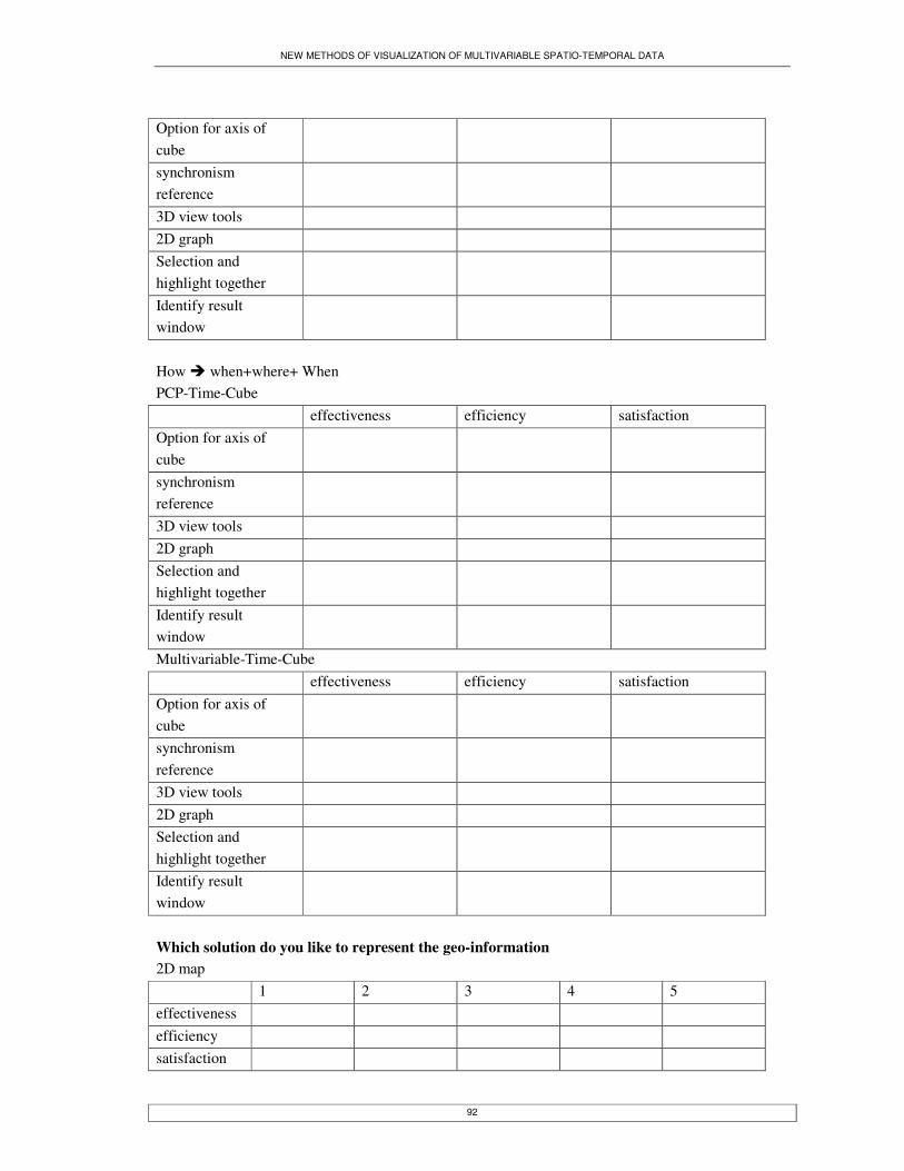
NEW METHODS OF VISUALIZATION OF MULTIVARIABLE SPATIO-TEMPORAL DATA
92
Option for axis of cube
synchronism reference
3D view tools 2D graph Selection and highlight together
Identify result window
How � when+where+ When PCP-Time-Cube effectiveness efficiency satisfaction Option for axis of cube
synchronism reference
3D view tools 2D graph Selection and highlight together
Identify result window
Multivariable-Time-Cube effectiveness efficiency satisfaction Option for axis of cube
synchronism reference
3D view tools 2D graph Selection and highlight together
Identify result window
Which solution do you like to represent the geo-information 2D map 1 2 3 4 5 effectiveness efficiency satisfaction
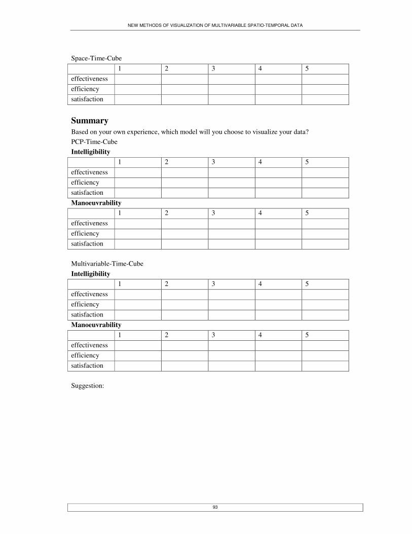
NEW METHODS OF VISUALIZATION OF MULTIVARIABLE SPATIO-TEMPORAL DATA
93
Space-Time-Cube 1 2 3 4 5 effectiveness efficiency satisfaction
Summary Based on your own experience, which model will you choose to visualize your data? PCP-Time-Cube Intelligibility 1 2 3 4 5 effectiveness efficiency satisfaction Manoeuvrability 1 2 3 4 5 effectiveness efficiency satisfaction Multivariable-Time-Cube Intelligibility 1 2 3 4 5 effectiveness efficiency satisfaction Manoeuvrability 1 2 3 4 5 effectiveness efficiency satisfaction Suggestion: