Embed Size (px)
Citation preview

MONETARY POLICY IN AN EQUILIBRIUMPORTFOLIO BALANCE MODEL
Michael Kumhof, International Monetary Fund
Stijn Van Nieuwerburgh, New York University
January 30, 2005
AbstractThis paper analyzes the general equilibrium effects of monetary policy choices on port-
folio shares of domestic and foreign currency denominated securities. Concentrating on thesmall open economy case, it relates the optimal choice of portfolio shares to the domestic-foreign interest rate differential. The first contribution of the paper is to show that there areindeed conditions under which a portfolio balance relationship holds in equilibrium, afterthe effects of government tax and spending policies have been endogenized. This has twoimportant implications. First, monetary policy can be shown to not only affect the level ofinflation via a target path for the nominal anchor, but also the volatility (and also the level) ofinflation via balance sheet operations. Most strikingly, sterilized intervention affects interestrates through its effect on inflation volatility. Second, this provides a theory of currency riskpremia and their endogenous determination by fundamentals and monetary policy, includinga determination of the conditions under which risk premia are or are not significant.
We identify two factors that affect the effectiveness of sterilized intervention. The firstis the prevalence of exogenous fiscal spending shocks, shocks that induce budget balancingexchange rate movements instead of being financed by endogenous tax responses. The sec-ond is the central bank’s initial balance sheet position - sterilized intervention has the largesteffects if the government has only issued small amounts of domestic currency denominateddebt. This suggests that the conditions that give rise to this type of imperfect asset substi-tutability are more likely to be observed in developing countries.
The authors thank Guillermo Calvo, Ken Judd, Carmen Reinhart, Ken Rogoff, Tom Sargent,Martin Schneider and Stephen Turnovsky for helpful comments.

1 INTRODUCTION
This paper analyzes the general equilibrium effects of monetary policy choices on
portfolio shares of domestic and foreign currency denominated securities. Concentrating on
the small open economy case, it relates the optimal choice of portfolio shares to the domestic-
foreign interest rate differential. The first contribution of the paper is to show that there are
indeed conditions under which a portfolio balance relationship holds in equilibrium, after
the effects of government tax and spending policies have been endogenized. This has two
important implications. First, monetary policy can be shown to not only affect the level of
inflation via a target path for the nominal anchor, but also the volatility (and also the level) of
inflation via balance sheet operations. Most strikingly, sterilized intervention affects interest
rates through its effect on inflation volatility. Second, this provides a theory of currency risk
premia and their endogenous determination by fundamentals and monetary policy, including
a determination of the conditions under which risk premia are or are not significant.
We identify two factors that affect the effectiveness of sterilized intervention. The first is
the prevalence of exogenous fiscal spending shocks, shocks that induce budget balancing
exchange rate movements instead of being financed by endogenous tax responses. The
second is the central bank’s initial balance sheet position - sterilized intervention has the
largest effects if the government has only issued small amounts of domestic currency
denominated debt. This suggests that the conditions that give rise to this type of imperfect
asset substitutability are more likely to be observed in developing countries.
The paper is motivated by a curious tension between economic theory and practice on the
question of sterilized intervention. Most notably in developing countries, central bankers
routinely intervene in foreign exchange markets with offsetting operations in domestic
currency debt, with the intention of affecting interest rates and real activity without changing
the money supply and therefore inflation. Their thinking might be taken to reflect older,
partial equilibrium versions of portfolio balance theory such as Branson and Henderson
2

(1985). But the economics profession, both theorists and empiricists, has been challenging
the validity of such models for some time. We begin by summarizing this critique, and then
develop our model.
The standard reference of modern open economy macroeconomics, Obstfeld and Rogoff
(1996), dismisses portfolio balance theory as partial equilibrium reasoning because it omits
the government budget constraint. This point is made most comprehensively in an important
paper by Backus and Kehoe (1989).1 They show that under complete asset markets, or
under incomplete asset markets and a set of spanning conditions, changes in the currency
composition of government debt require no offsetting changes in monetary and fiscal policies
to both meet the government budget constraint and to leave private budget constraints
unaffected. Consequently this ’strong form’ of intervention is irrelevant for equilibrium
allocations and prices. This result does not depend on Ricardian equivalence, monetary
neutrality, or the law of one price, and can be shown using only an arbitrage condition.
The authors then go on to argue that weaker forms of government intervention in asset
markets generally require offsetting changes in monetary and/or fiscal policies to meet the
government budget constraint. Because the impact of such ’weak form’ interventions can
as easily be attributed to these monetary and/or fiscal changes as to the intervention per se,
sterilized intervention cannot be considered a separate, third policy instrument.
When the question of the efficacy of sterilized intervention is posed in this most general
form, the results of Backus and Kehoe (1989) are very powerful. However, as these authors
point out themselves, this leaves open the narrower but practically very important question
of precisely how ’weak form’ interventions affect the economy. The answer to this question
requires taking a stance on the precise form of other government policies. In this context, one
important consideration is that fiscal policy is generally not used as a short-term instrument
1 Other related references include: Sargent and Smith (1988) on the irrelevance of openmarket operations in foreign currencies; Chamley and Ptolemarchakis (1984), Sargent andSmith (1987), and Wallace (1981) on the irrelevance of domestic open market operations.
3

to affect asset market equilibria. It is therefore plausible to rule out fiscal behavior that
can respond arbitrarily to asset market interventions, and instead to consider only tax and
spending rules whose form is independent of such interventions. We can then ask how
sterilized intervention affects equilibrium allocations and prices conditional on the precise
form of these rules. In other words, we ask whether sterilized intervention is effective as
a second independent instrument of monetary policy. This is in fact a nontrivial exercise,
because several papers such as Obstfeld (1982) and Grinols and Turnovsky (1994) have given
a negative answer to that question. They show that, once a monetary policy rule such as a
money growth rule is specified, sterilized intervention has no further effects on asset market
equilibria. In their models domestic and foreign bonds are perfect substitutes in general
equilibrium, so that a version of uncovered interest parity holds. In this paper we show
that these results depend on the specific form of the fiscal policy rule used by these authors,
namely lump-sum redistribution of all government net revenue, and complete absence of
exogenous fiscal spending. While this is a convenient and frequently used assumption, it is
also very strong, and we contend that in many real world cases it is not very descriptive of
actual government behavior. When it is replaced by assuming at least some exogenous fiscal
spending, sterilized intervention can become an effective second instrument of monetary
policy. Our paper explores the nature of its effects in general equilibrium.
The model assumes stochastic processes for the nominal money supply, velocity, real
returns on internationally tradable assets, and government spending. All of these processes
generate nominal exchange rate volatility. Domestic currency denominated government debt
securities therefore generate a stochastic seigniorage flow, and in partial equilibrium this
would give rise to currency risk for private asset holders. But in general equilibrium, fiscal
policy, or in other words the use of this seigniorage by the government, is critical. In the
case of full lump-sum redistribution to households, we will confirm the well-known result
that currency risk is absent in general equilibrium and that uncovered interest parity must
hold. But that assumption is not available for exogenous fiscal spending. As long as such
4

spending is not a perfect substitute for private spending, we can then show that in this case
domestic currency denominated government bonds are risky even in general equilibrium.
They are imperfect substitutes for foreign currency denominated bonds and their portfolio
share is determined by a portfolio balance equation.
The focus of this paper on emerging markets is also justified on empirical grounds. As
mentioned above, economists have questioned the effectiveness of sterilized intervention
not only theoretically but also empirically. Edison (1993) is a good summary of the latter,
but her evidence is limited to developed countries. The evidence for emerging markets
summarized by Montiel (1993) is thinner but it does suggest some effectiveness of sterilized
intervention. A key precondition for this is imperfect substitutability between domestic
and foreign currency denominated bonds. An important paper by Bansal and Dahlquist
(2000) presents valuable and more recent evidence on this question. These authors find high
currency risk premia in emerging markets, and show that country-specific risk factors are
much more important than systematic portfolio risk factors in explaining the cross-country
variation is risk premia. Our model explores one important country-specific risk factor, fiscal
spending volatility. Gavin and Perotti (1997) document that Latin American countries do
indeed exhibit much more fiscal volatility than OECD countries.
Our paper is related to a large theoretical literature trying to explain nominal interest
rate risk premia. These are generally decomposed into default risk premia and currency
risk premia. While there is a well-established and growing literature on interest rate default
risk premia2, currency risk is a less straightforward notion. Engel (1992) and Stulz (1984)
show that in flexible price monetary models monetary volatility per se will not give rise to
a risk premium. Engel (1999), using the frameworks of Obstfeld and Rogoff (1998, 2000)
and Devereux and Engel (1998), shows that sticky prices are required to generate a risk
premium. However, the terms that he identifies as being able to generate risk premia are
2 The early contributions include Eaton and Gersovitz (1981) and Aizenman (1989). Morerecent contributions include Kehoe and Perri (2001) and Kletzer and Wright (2000).
5

generally empirically small in industrialized countries. In developing countries this may be
different, but the added difficulty there is to distinguish currency risk premia or discounts
from sometimes large default risk premia.
Our theory suggests an alternative explanation that depends on the fundamentals of fiscal
policy, and that has very different implications for monetary policy, specifically the ability of
central bank sterilized intervention to affect interest rates and allocations. In a flexible price
setting, it generates a risk discount due to a Jensen’s inequality term.3 We show that this term
can in fact be very small if the government has issued a large amount of nominal debt, and
if exogenous fiscal spending volatility is small, as may be the case in many industrialized
countries. This would be consistent with the empirical evidence mentioned by Engel (1999).
But in the opposite scenario this discount can be of the order of several hundred basis points,
and it can give the government significant scope for balance sheet operations. The fact that
in many developing countries one often observes an overall risk premium is likely to be due
to the interaction of discounts of the kind we emphasize with borrowing risk premia and with
Peso-problem type premia of the kind emphasized by Obstfeld (1987).
The rest of the paper is organized as follows. Section 2 presents the model. Section 3
presents an illustrative example of the model’s results and policy implications using Mexican
data. Section 4 concludes. Mathematical details and details of the data used are presented in
a number of appendices.
2 The Model
Consider a small open economy composed of a continuum of identical infinitely
lived households and a government. Households’ consumption ct is financed from a
constant endowment stream y4 and from the returns on three types of financial assets,3 It also incorporates a borrowing risk premium. While this could be used for some interestingpolicy experiments, in this paper it will only be used to complete the model and to rule outinterest rate indeterminacy at extremely high levels of government borrowing.4 The endowment stream is not strictly necessary for the theoretical model. But it is critical
6

domestic currency denominated money Mt with a zero nominal return, domestic currency
denominated bonds Qt with a nominal return iqtdt, and internationally tradable assets bt with
a real return drbt . The nominal exchange rate Et floats. Aggregate exchange rate risk cannot
be hedged through financial instruments.5 We will see that this may, but need not, imply that
financial markets are incomplete. All goods are tradable and the international price level is
normalized to one. Assuming purchasing power parity, domestic goods prices Pt therefore
satisfy Pt = Et. Nominal variables are denoted by upper case letters and real variables in
terms of tradable goods by lower case letters.
We use a continuous time stochastic monetary portfolio choice model to derive
households’ optimal consumption and portfolio decisions.6 In order to determine the
equilibrium portfolio share of domestic currency denominated assets in a small open
economy, we follow Grinols and Turnovsky (1994) in assuming that these bonds are held
exclusively by domestic residents. This is not a restrictive assumption for many emerging
markets, where the vast majority of claims by foreigners tends to be denominated in dollars.
Figure 1 illustrates this for the case of Mexico, the country that we will use later for a
calibration of the model’s shock processes.
2.1 Shock Processes
We fix a probability space (Ω,z, P ). A stochastic process is a measurable function Ω
× [0,∞) : 7→ <. The value of a process X at time t is the random variable written as
Xt. We define a three-dimensional Brownian motion Bt = [BMt Bα
t Brt ]0, consisting
for the computed example in Section 3.5 This requires that the risk of the domestic currency is too idiosyncratic to be internationallydiversifiable, or that that market is too small relative to transactions costs. Both are plausiblefor emerging markets. Of course individual households can hedge domestically if there isheterogeneity among them. But what matters is that households as a whole cannot hedgetheir aggregate domestic currency exposure vis-a-vis their own government.6 Useful surveys of the technical aspects of stochastic optimal control are contained in Chow(1979), Fleming and Rishel (1975), Malliaris and Brock (1982), Karatzas and Shreve (1991), andDuffie (1996). The seminal papers using this technique to analyze macroeconomic portfolioselection are Merton (1969, 1971) and Cox, Ingersoll and Ross (1985). Other contributionsinclude Dumas and Uppal (2000), Grinols and Turnovsky (1994), and Stulz (1983, 1984, 1987, 1988).
7

of shocks BMt to the growth rate of the nominal money supply, shocks Bα
t to the growth
rate of consumption velocity αt = ct(Mt/Et)
, and shocks Brt to the real return on tradable
assets drbt . We also define a one-dimensional Brownian motion Wt that represents shocks
to the growth rate of government spending dgt. We employ different notation for this shock
because, compared to Bt, it assumes a different transmission channel between money and
the exchange rate. This difference is critical for our results.
Specifically, all shocks affect the return properties of domestic currency denominated
assets through the exchange rate, and this has repercussions for the government budget
constraint. The difference between Bt-shocks and Wt-shocks is the nature of the fiscal
response. We assume that with respect to Bt-shocks the fiscal policy response is
endogenous. This means that the government redistributes the net fiscal balance resulting
from financial transactions back to households via lump-sum transfers. But Wt-shocks are
by assumption exogenous shocks to fiscal policy, and here we assume that the exchange
rate adjusts to balance the government’s budget. This in turn implies that monetary
policy is endogenous, specifically that money is allowed to accommodate the exchange rate
movements necessitated by fiscal balance.
The nominal money supply follows a geometric Brownian motion with drift process µtdetermined by monetary policy, a constant, exogenous three dimensional diffusion σM =
[σMM σαM σrM ] with respect to Bt-shocks, an endogenous diffusion σgM,t with respect to
Wt-shocks:dMt
Mt= µtdt + σMdBt + σgM,tdWt . (1)
Here we index endogenous drift and diffusion terms by time if they represent possibly time-
varying monetary policy choices, or if they are functions of such choices. Finally, we will
at a later stage allow for unanticipated, one-off and discontinuous shocks to the stock of
money ∆Mt. This will be required to discuss the effects of unsterilized foreign exchange
interventions and of domestic open market operations. That discussion will be useful to
decompose the effects of sterilized foreign exchange interventions. For the latter, the main
8

topic of this paper, money follows equation (1) without any discontinuities.
The process for velocity is similar, except of course in that velocity does not endogenously
respond to fiscal shocks:dαt
αt= νdt + σαdBt . (2)
The real return on tradable assets follows a process
drbt = rdt + σrdBt . (3)
It is assumed that the exogenous components of the stochastic processes d log(Mt), d log(αt)
and drbt are correlated, with a variance-covariance matrix Σ. Finally, government spending
follows a process for which shocks are assumed to be uncorrelated with Bt-shocks:dgtat
= gdt + σggdWt . (4)
A critical feature of fiscal spending shocks is that they are assumed to introduce a real risk
for holders of government liabilities because of their implications for the government budget.
For this risk to matter in general equilibrium, it must be true that government consumption is
an imperfect substitute for private consumption. We choose the simplest and most tractable
assumption under which this is true, namely government spending does not enter household
utility at all.
The tribe zBWt includes every event based on the history of the above four Brownian
motion processes up to time t. We complete the probability space by assigning probabilities
to subsets of events with zero probability. We definezt to be the tribe generated by the union
of zBWt and the null sets. This leads to the standard filtration z = zt : t ≥ 0.
The nominal exchange rate process Et is endogenously determined as a function of the
four exogenous stochastic processes. It follows a geometric Brownian motion, with its drift
εt and diffusions σE and σgE,t to be determined in equilibrium:dEt
Et= εtdt + σEdBt + σgE,tdWt . (5)
We assume and later verify that the endogenous drift and diffusion terms are adapted
processes satisfyingR T0|εt|dt < ∞ almost surely for each T , and
R T0
(σxE)2 dt < ∞
9

(x = M,α, r),R T0
¡σgE,t
¢2dt < ∞ almost surely for each T . The corresponding conditions
for all exogenous or policy determined drift and diffusion processes hold by assumption -
the exogenous terms are constants and policy choices µt are assumed to be bounded.
In the ensuing analysis we will use the following shorthand notation for diffusion terms,
choosing terms relating to exchange rates and money as the example:
(σE)2 =¡σME¢2
+ (σαE)2 + (σrE)2 ,
σMσE = σMMσME + σαMσαE + σrMσrE ,
(σM − σE) = [¡σMM − σME
¢(σαM − σαE) (σrM − σrE)] .
2.2 Households
The representative household has time-separable logarithmic preferences7 that depend on
his lifetime stochastic path of tradable goods consumption ct∞t=0. It is convenient to model
period utility in terms of consumption in excess of the constant endowment stream y. We
therefore have
E0
Z ∞
0
e−βt ln(ct − y)dt , 0 < β < 1 , (6)
where β is the rate of time preference. We denote the real stocks of money and domestic
bonds bymt = Mt/Et and qt = Qt/Et, and total private financial wealth by at = bt+qt+mt.
Portfolio shares of money and domestic bonds will be denoted by nmt
= mt
atand nq
t= qt
at.
Finally, households are subject to a lump-sum tax dTt levied as a proportion of wealth and
following an Itô process with adapted drift process τ t and diffusion process σTt :
dTtat
= τ tdt + σT,tdBt . (7)
The drift and diffusion terms will be determined in equilibrium from a balanced budget
requirement for the government. Note that taxes respond to Bt-shocks but not to Wt-shocks.
We assume thatR T0|τ t|dt < ∞ almost surely for each T and
R T0
(σT,t)2 dt < ∞ almost
7 Logarithmic preferences are commonly assumed in the open economy asset pricing andportfolio choice literature for their analytical tractability, see e.g. Stulz (1984, 1987) and Zapatero (1995).
10

surely for each T , and will later verify that this is satisfied in equilibrium. The household
budget constraint is given by
dat = at£nmt dr
mt + nq
tdrqt + (1− nm
t− nqt )dr
bt
¤+ydt−ctdt−at[τ tdt+σT,tdBt]−Γt , (8)
where drit is the real rate of return on asset i. The final term Γt represents a risk-premium on
international borrowing, specified as
Γt = Iγat(nmt + nqt − φ)2 , (9)
where I is an index, with I = 1 if (nmt + nqt ) > φ and I = 0 otherwise. Intuitively, as
the government expands its debt stock so that (nmt + nqt ) rises, households have to sell part
of their internationally tradable assets to the central bank to purchase government liabilities.
Beyond some level φ of government borrowing, households have to start borrowing from
foreigners in order to finance their domestic debt holdings. At that point foreigners demand
a risk premium.8 The assumption of international borrowing costs that depend on the level
of foreign indebtedness has become commonplace in the open economy macroeconomics
literature. We will follow the convention in that literature, which is based on empirical
evidence, to assume a small risk premium γ. While the risk premium channel could be used
to generate interesting results of its own for portfolio decisions, in our paper it is mainly
adopted for technical reasons. Specifically, it rules out degenerate behavior of the interest
rate at extremely high levels of foreign borrowing. At more realistic levels of borrowing
we will see that the key driving force of portfolio behavior is endogenous exchange rate
volatility. It remains to specify the critical level φ. A strict interpretation of the model
requires φ = 1, based on the fact that there is no formal limit to sales of internationally
tradable assets in the model. A more flexible and realistic assumption realizes that any
aggregate net international asset position reflects many offsetting gross positions, meaning
gross international borrowing positions will occur at φ < 1. In any event, given a choice of
γ near zero the assumption about φ does not dominate the final results.8 Foreigners therefore do not take into account the government’s net asset position whenlending to the country’s private sector.
11

Many monetary portfolio choice models introduce money into the utility function
separably because this preserves the separability between portfolio and savings decisions
found in Merton (1969, 1971). However, as pointed out by Feenstra (1986), without
a positive cross partial between money and consumption the existence of money cannot
be rationalized through transactions cost savings. We therefore use a cash constraint
instead, and show that it is nevertheless possible to obtain very elegant analytical solutions.
Specifically, consumers are required to hold real money balances equal to a time-varying
multiple αt of their consumption expenditures:
ct = αtmt = αtnmt at . (10)
The now very common treatment of the cash-in-advance constraint in Lucas (1990) has
two aspects, a cash requirement aspect and an in-advance aspect. Our own treatment goes
back to the earlier Lucas (1982), which uses only the cash requirement aspect. This is due
to the difficulty of implementing the in-advance timing conventions in a continuous-time
framework. In the continuous time stochastic finance literature, Bakshi and Chen (1997)
have used the same device. Finally, note that equation (10) could also be obtained as an
optimality condition by assuming Leontief preferences over consumption and real balances,R∞0
e−βt ln(min(ct, αtmt))dt.
Using Itô’s lemma we can derive the real returns in terms of tradable goods on money and
domestic bonds (see Appendix I):
drmt =³−εt + (σE)2 +
¡σgE,t
¢2´dt− σEdBt − σgE,tdWt , (11)
drqt =³iqt − εt + (σE)2 +
¡σgE,t
¢2´dt− σEdBt − σgE,tdWt . (12)
Note that the exchange rate affects returns in two ways. First, depreciation σEdBt > 0
reduces the ex-post real value of nominal domestic assets in terms of tradables. Second, by
Jensen’s inequality, larger exchange rate volatility (σE)2 increases their ex-ante real return.
12

The household’s portfolio problem is to maximize present discounted lifetime utility by
the appropriate portfolio choice nmt , nqt∞t=0:
maxnmt ,nqt∞t=0
½E0
Z ∞
0
e−βt ln¡αtn
mtat − y
¢dt
¾s.t.
dat = at©(r − τ t − γI(nmt + nqt − φ)2)dt (13)
+nmt
h(−αt − r − εt + (σE)2 +
¡σgE,t
¢2)dt− σEdBt − σgE,tdWt
i+nq
t
h(iqt − r − εt + (σE)2 +
¡σgE,t
¢2)dt− σEdBt − σgE,tdWt
i+(1− nmt − nqt )σrdBt − σT,tdBt .
We will solve this optimal portfolio problem recursively using a continuous time Bellman
equation, as in Merton (1969, 1971). Let V (at, t) = e−βtJ(at, t) ∈ C2 be a solution of the
Hamilton-Jacobi-Bellman equation of stochastic optimal control. Let J = ∂J(at, t)/∂t.
Then the Hamilton-Jacobi-Bellman equation is
βJ − J = supnmt ,nqt
©ln¡αtn
mtat − y
¢+ Jaat[
¡r − τ t − γI(nmt + nqt − φ)2
¢(14)
+nmt
³−αt − r − εt + (σE)2 +
¡σgE,t
¢2´+ nq
t
³iqt − r − εt + (σE)2 +
¡σgE,t
¢2´]
+1
2Jaaa
2t
h¡nmt
+ nqt
¢2 ³(σE)2 +
¡σgE,t
¢2´+¡1− nm
t− nq
t
¢2(σr)
2 + (σT,t)2
−2¡nmt
+ nqt
¢σEσr + 2
¡nmt
+ nqt
¢2σEσr
+2¡nmt
+ nqt
¢σEσT,t − 2
¡1− nm
t− nq
t
¢σrσT,t
¤ªwith boundary condition
limτ→∞
E0
£e−βτ |J(aτ , τ)|
¤= 0 . (15)
Optimality for nqt
requires
nqt+ nm
t=
³−JaJaaat
´³iqt − r − εt + (σE)2 +
¡σgE,t
¢2´³(σE)2 +
¡σgE,t
¢2+ (σr)
2 + 2σEσr
´ (16)
13

+(σr)
2 + σEσr + 2γ³
JaJaaat
´I (nmt + nqt − φ)− σEσT,t − σrσT,t³
(σE)2 +¡σgE,t
¢2+ (σr)
2 + 2σEσr´ ,
This expression is not yet in a very informative form, as we first need to solve for
equilibrium taxation. On the other hand, the first-order condition for nmt
is straightforward:1
αtnmt at − y= Ja(1 +
iqtαt
) . (17)
The marginal utility of consumption equals the marginal utility of wealth Ja times the
effective price of consumption, where the latter varies with the opportunity cost of holding
money balances for transactions purposes. A closed form solution for J , which is required to
get an explicit expression, will be derived following the endogenization of taxes in the next
section, and following the definition of equilibrium.
2.3 Government
Monetary policy is characterized by two policy variables and by a technical condition on
the government budget.
Primary control over the level of inflation is achieved through a target path for the nominal
anchor consistent with an inflation target. In the present, flexible price model this is a target
path µt∞t=0 for money in equation (1). The diffusion process σM in that equation is assumed
to be constant and exogenous - the government needs to allow mean zero shocks to the
money supply to accommodate exogenous financial market shocks that may or may not be
correlated with shocks to velocity or interest rates. On the other hand, the diffusion process
σgM,t is endogenous and determined in equilibrium. Finally, being an Itô process, Mt is
continuous, which ensures exchange rate determinacy.
We will show that control of the volatility of inflation can be achieved by setting a target
path for the stock of nominal government debt Qt∞t=0. We will also see that under our
assumptions, particularly that of a risk premium at very high levels of government debt
issuance, there is a monotonic relationship between Qt and iqt for all iqt > 0, so that there
is an equivalent target path for the nominal interest rate on government debt.iqt∞t=0. As it
14

turns out, this target also has a secondary effect on the level of inflation. To show that the
government can indeed control iqt independently of µt requires that we find a determinate
portfolio demand share for domestic currency bonds nqt in equation (16), after endogenizing
fiscal policy. The first major objective of this paper is to clarify the conditions under which
that is possible. If it is possible, it becomes meaningful to consider separately the effects of,
first, unsterilized foreign exchange intervention, second, domestic open market operations,
and third, sterilized foreign exchange intervention as a combination of the first two. That
analysis will contain the main policy relevant conclusions of the paper.
Finally, we need a technical condition on the government budget. Discrete unanticipated
policy changes will generally result in discontinuous jumps of the nominal exchange rate
on impact9, denoted E0 − E0−. Here 0− stands for the instant before the announcement of
a new policy at time 0. At such points the government could either spend the associated
net seigniorage revenue, or it could fully redistribute it through a one-off transfer of
internationally tradable assets. We assume the latter, and this ensures that private financial
wealth remains unchanged upon the impact of any new policy. We denote internationally
tradable assets held by the government as ht, and we denote asset transfers to compensate
exchange rate jumps by ∆h0 = −∆b0.10 Then we can formalize the above as
(M0− + Q0−)
µ1
E0− 1
E0−
¶= −∆b0 = ∆h0 . (18)
Next we consider fiscal policy. The exogenous, spending component of fiscal policy is
specified in (4) and the endogenous, lump-sum tax component in (7). We assume that the
latter meet three requirements. First, the expected budget balance is always zero. Second,
the budgetary effects of shocks to money, velocity and international interest rates, Bt-shocks,
are exactly offset by lump-sum taxes. Third, in order for the assumption of exogeneity of
spending shocks gt in (4) to be meaningful, endogenous lump-sum taxes do not adjust to
9 Subsequent discontinuous exchange rate jumps are ruled out by arbitrage.10 Note that ∆h0 need not equal h0 − h0−, because the policy itself may in addition involve thepurchase or sale of foreign exchange reserves against domestic money or bonds at the new exchange rateE0.
15

react to these shocks. Instead, the budget balancing role in response to such shocks falls to
the exchange rate.
The government’s budget constraint is
atτ tdt + atσT,tdBt + htdrbt = mtdr
mt + qtdr
qt + dgt . (19)
The assumption of budget balance together with (18) imply that the government’s net
wealth Wt = ht −mt − qt does not change over time:
dWt = dht − dmt − dqt = 0 .
Therefore we have dht = dmt + dqt. For simplicity we also assume the initial condition
W0− = 0, or
h0− = m0− + q0− , (20)
which implies that
ht = mt + qt ∀t . (21)
This formulation treats government issued and central bank issued domestic currency
bonds as perfect substitutes, so that qt could represent either debt class. Condition (21)
therefore states that the consolidated government’s net domestic currency denominated
liabilities are fully backed by internationally tradable assets.11 It should also be pointed
out that, given perfect international capital mobility, the assumption of instantaneous
redistribution in (19) is not restrictive. It is equivalent to redistribution over households’
infinite lifetime combined with instantaneous capitalization by households of the expected
redistribution stream. Our treatment is analytically more convenient.
To determine the drift τ t and diffusion σT,t of the tax process dTt, and the diffusion σgE,t
of the exchange rate process, we equate terms in (19) using (11), (12), (3) and (21), and we
use our above three requirements for lump-sum taxes. We obtain the following:
τ t = nqtiqt −
¡nmt
+ nqt
¢ ³r + εt − (σE)2 −
¡σgE,t
¢2´, (22)
11 Note that qt could be negative and represent government claims on the private sector. Inthat case ht could also be negative.
16

σT,t = −(nmt
+ nqt) (σE + σr) , (23)
σgE,t =σgg
(nmt
+ nqt). (24)
The first condition ensures that the expected budget balance is always zero. The second
condition represents the endogenous response of lump-sum taxes to Bt-shocks. The third
condition is critical for our results. It represents the endogenous response of the exchange
rate to Wt-shocks. Fiscally induced exchange rate volatility depends on the volatility
of the fiscal shocks themselves, but it is decreasing in the amount of domestic currency
denominated liabilities the government has succeeded in issuing. This is because the base of
the ‘inflation tax’, the stock of nominal liabilities that can be revalued by nominal exchange
rate movements, is larger in that case. As we will see, raising the amount of domestic
currency denominated liabilities requires a higher interest rate. In other words, a higher
interest rate is (ceteris paribus) associated with lower exchange rate volatility and therefore
inflation volatility.
2.4 Equilibrium and Balance of Payments
We define a government policy as a list of stochastic processes12 µt, iqt , τ t, σT,t∞t=0
and an initial net compensation ∆h0 such that, given a list of stochastic processes
εt, σE, σgE,t, nmt , nqt∞t=0, initial conditions b0−, h0−,M0−, Q0− and E0−, and an initial
exchange rate jump E0 − E0−, the conditions (22), (23), (24) and (18) hold at all times.
Then equilibrium is defined as follows:
An equilibrium is a set of initial conditions b0−, h0−,M0−, Q0− and E0−, exogenous sto-chastic processes Bt,Wt∞t=0, an allocation consisting of stochastic processesct, bt, ht, Qt,Mt∞t=0, a price system consisting of an initial exchange rate jump E0 −E0− and stochastic processes εt, σE, σgE,t∞t=0, and a government policy such that,given the initial conditions, the exogenous stochastic process, the government policy
12 In all policy experiments we will assume for simplicity that µt, iqt∞t=0 are deterministic sequences.
17

and the price system, the allocation solves households’ problem of maximizing (6) sub-ject to (8) and (10), resulting in optimality conditions (16) and (17).
The condition ht = mt + qt ∀t ensures that at = bt + ht ∀t, i.e. internationally tradable
private assets at any point are equal to the economy’s net internationally tradable assets.
Then the current account can be derived by consolidating households’ and the government’s
budget constraint (8) and (19).
dat = ratdt + ydt− ctdt + atσrdBt − atσggdWt − atγI(n
mt + nqt − φ)2 . (25)
We are now ready to derive a closed form expression for the household value function.
The solution proceeds by first substituting (16), (17), (22) and (23), which contain the terms
Ja and Jaa, back into the Hamilton-Jacobi-Bellman equation (14). That equation is then
solved for J by way of a conjecture. Given our specification of the utility function a good
conjecture is
J(at, t) = X [ln(at) + ln(Y (t;xt))] , (26)
where X and Y (t;xt) are to be determined in the process of verifying the conjecture, and
where xt =©µt, i
qt ,Mt, αt, r
bt , gt
ª. Thus, the conjecture allows for Y (.) to be a function
of both time and of the economy’s exogenous policy and shock processes. To understand
this note that the value function represents the present discounted value of expected future
consumption streams. First-order condition (17) together with (25) implies that consumption
at t is decreasing in iqt , increasing in αt, and proportional to at, where the latter in turn is a
function of the full set of exogenous policy and shock processes of the economy. The same
is true for expected future consumption, given the Brownian nature of shock increments.
In Appendix II we first show that (26) implies
X = β−1 . (27)
Therefore, using (22) and (23), the first-order conditions (16) and (17) become
nqt+ nm
t=
³iqt − r − εt + (σE)2 +
¡σgE,t
¢2+ (σr)
2 + σEσr + 2γI´
³¡σgE,t
¢2+ 2γI
´ , (28)
18

ct = y +βat
(1 + (iqt/αt)). (29)
Equation (29) is a standard condition in this model class. It states that consumption in
excess of the flow endowment is proportional to wealth and, because of the cash constraint,
negatively related to nominal interest rates. It is equation (28), the key equation of this
paper, that distinguishes this model from other open economy models. What is says is that
the portfolio share of domestic currency denominated assets is determinate, even after taxes
have been endogenized. In the following discussion we will pass over the risk premium
term 2γI, which in our calibration is both very small and which only enters at very high
levels of government borrowing. Assume for a moment that the volatility of exogenous
fiscal spending is zero (σgg = 0). Then (28) in conjunction with (24) would imply that
iqt = r + εt − (σE)2 − (σr)2 − σEσr . (30)
Endogenizing taxes in the absence of exogenous fiscal spending therefore results in a version
of uncovered interest parity, the only difference being Jensen’s inequality terms relating
to exchange rate and interest rate volatility. Crucially, the portfolio share (nmt + nqt ) is
indeterminate. In such a model the exchange rate drift would be fully determined by money
growth, exchange rate volatility would be fully determined by exogenous Bt-shocks, and
there would be no scope for monetary policy to choose a second policy instrument such
as the interest rate iqt (or the stock of domestic bonds Qt). The currency composition of
central bank balance sheets would not matter. Versions of this result have been found in
other papers, such as Grinols and Turnovsky (1994) and Kumhof and Van Nieuwerburgh
(2003). The reason for this result is that full lump-sum redistribution of the net seigniorage
consequences of shocks fully insures agents against exchange rate risk in general equilibrium
- the absence of a market for hedging exchange rate risk is immaterial. Private agents may
lose from exchange rate movements at the expense of the government, but the economy as a
whole does not, and therefore neither do private agents after the government returns to them
19

what it gained at their expense.
With exogenous fiscal spending shocks the situation is entirely different. A spending
shock dWt > 0 is a net resource loss to the economy because government spending does not
enter private utility. Furthermore, the government passes this loss on to holders of domestic
currency denominated assets through exchange rate movements. This risk of nominal
exchange rate changes, the source of which is in fact real, is the source of imperfect asset
substitutability. Equation (28) shows that the government can induce agents to expand their
portfolio share of domestic currency denominated liabilities by offering (ceteris paribus) a
higher interest rate. And by equation (24) the higher portfolio share implies that a given fiscal
spending volatility translates into a lower inflation volatility because the base of this ‘inflation
tax’ is higher. Because inflation volatility increases the mean return of domestic currency
denominated assets by (11) and (12), interest rates have to rise more strongly the more
they induce substantial reductions in inflation volatility. The final result is a monotonically
increasing relationship between domestic interest rates and the portfolio share of domestic
currency denominated assets. The following subsection develops the mathematics behind
this argument in more detail.
2.5 Equilibrium Exchange Rate Dynamics
Equilibrium exchange rate dynamics can be determined by noting that consumption has
to satisfy two conditions in equilibrium. The first is the cash-in-advance constraint (10), and
the second the consumption optimality condition (29). The latter in turn links the evolution
of consumption to the evolution of assets, and therefore needs to be analyzed in conjunction
with equation (25).
We begin with (10). By Itô’s Law, the cash-in-advance constraint can be stochastically
differentiated as
dct = αtdmt + mtdαt + dmtdαt . (31)
20

Again by Itô’s Law, real money balances evolve as follows:
dmt = mt
hµt − εt + (σE)2 +
¡σgE,t
¢2 − σMσE − σgMσgE,t
idt (32)
+mt [σM − σE] dBt + mt
£σgM − σgE,t
¤dWt .
We substitute (32), (2) and (10) into (31) to obtain the following evolution of
consumption:
dctct − y
(33)
=hµt − εt + ν + (σE)2 +
¡σgE,t
¢2 − σMσE − σgMσgE,t + σασM − σασEidt
+ [σM − σE + σα] dBt +£σgM − σgE,t
¤dWt .
We rewrite the consumption optimality condition (29) as follows:
zt = (ct − y) (1 + (iqt/αt))− βat ≡ 0 . (34)
We differentiate this condition using Itô’s Law to obtain
∂zt∂ct
dct +∂zt∂αt
dαt +∂zt∂at
dat +1
2
∂2zt∂α2
t
(dαt)2 +
∂2zt∂ct∂αt
(dctdαt) = 0 . (35)
For aggregate asset evolution, we substitute (29) into (25) to get
dat = at
∙r − β
(1 + (iqt/αt))
¸dt + atσrdBt − atσ
ggdWt − atγI(n
mt + nqt − φ)2dt ,
while velocity evolution is given by (2). Substituting these terms into (35) and
simplifying, we obtain the following expression for the evolution of consumption:
dctct − y
(36)
=
∙µr − β
(1 + (iqt/αt))
¶+
µiqt
αt + iqt
¡ν − (σα)
2¢¶− γI(nmt + nqt − φ)2
¸dt
+
∙σr +
iqtαt + iqt
σα
¸dBt − σggdWt +
∙iqt
αt + iqt(νdt + σαdBt)
¸dct
ct − y
To obtain the equilibrium exchange rate dynamics, we substitute (33) into (36) and
separately equate the terms multiplying dt, dBt and dWt. For simplicity denote the share
of domestic currency denominated assets in private portfolios as nt = nmt + nqt . Then, given
21

αt and at, the following is the equilibrium system of 10 equations that determines the 10
variables nt, εt, σE = [σME σαE σrE], σgE,t, σgM,t, ct, Et, and either Mt or Qt, given either Qt
or Mt:
nt =iqt − r − εt + (σE)2 +
¡σgE,t
¢2+ (σr)
2 + (σrσE) + 2γI¡σgE,t
¢2+ 2γI
, (37)
µt + ν − εt + (σE)2 +¡σgE,t
¢2 − σMσE − σgM,tσgE,t + σασM − σασE (38)
=
µr − β
(1 + (iqt/αt))
¶+
µiqt
αt + iqt(ν + σασM − σασE)
¶− γI(nt − φ)2 ,
σM + σα − σr − σE =iqt
αt + iqtσα , (39)
σgM,t − σgE,t + σgg = 0 , (40)
σgE,t =σggnt
, (41)
αtMt = Etct , (42)
ct = y +βat
(1 + (iqt/αt)), (43)
nt =Mt + Qt
Et. (44)
We assume and later verify, for a specific calibration of the exogenous shock processes,
that this system has a unique solution for a bounded setting of the policy variables µt and
iqt , and given constant exogenous drift and diffusion processes of the economy’s four shock
processes.13 This means that all endogenous variables including nt can be written uniquely
in terms of the exogenous policy and shock processes. This verifies the regularity conditions13 It can be shown that in certain borderline cases the solution may in fact not be unique, specifically whennt > 1 and γ −→ 0. We can rule out such cases by choosing a sufficiently positive but still very small γ. Butin general, it can also be shown that uniqueness can in such cases be reestablished if the government choosesas its second policy instrument the nominal stock of bonds Q instead of the interest rate on those bonds iq.
22

posited earlier for εt, σE, σgE,t, τ t and σT,t. It is also needed to verify that our conjectured
value function and resulting policy functions for nmt and nqt solve the Hamilton-Jacobi-
Bellman equation. The steps of that verification are shown in Appendix II.
3 Policy Implications
3.1 An Illustrative Example
To analyze the properties of the model we now turn to data for Mexico, a small open
economy with a substantial outstanding stock of domestic currency denominated liabilities.
We use quarterly data from the first quarter of 1996 through the second quarter of 2004 (34
observations) to estimate the drifts and variance-covariance matrix of the economy’s four
shock processes. We then go on to show what these data imply for the behavior of inflation
and taxation under different assumptions about government balance sheet operations and
therefore interest rates. In doing so we will hold constant the calibrated parameters β = 0.04,
y = 1, φ = 0.5 and γ = 0.0001.14
This is a highly stylized model economy, and some of its key features have no easily
identifiable counterpart in the data. In addition to estimating the shock processes, we
therefore need to make some reasonable assumptions and approximations. The following
exercise, while guided by the data, is therefore best seen as illustrative of our theoretical
results. Most importantly, consumption in the model is financed from both an endowment
income and from income on financial assets, see equation (29). We assume that the fraction
x of the latter in overall consumption spending is x = 0.02 on average. As we will see,
this has reasonable implications in the light of Mexican national accounts and government
liabilities data. Given our normalization y = 1, this implies a model-consistent relationship
between average consumption c and average national wealth a, which is useful because no
14 The last two assume that a borrowing premium starts to apply when households have investedhalf their financial wealth in government securities, but that the premium is extremely small.
23

reliable data exists for the latter. Specifically, a = cx/β.15
The key shock process in the model is the volatility of fiscal spending, and all spending
shocks are assumed to be exogenous, in other words to have no endogenous tax response.
This will generally not be true in the data, see Canzoneri, Cumby and Diba (2004) on the
difficulties of distinguishing fiscally dominant and monetary dominant policies in the data.
We therefore need to make an assumption about the fraction z of observed fiscal spending
volatility that is exogenous. We assume z = 0.0225 to get a set of benchmark results for
Mexico, but we also explore the sensitivity of our results to other assumptions, given that
this is a critical parameter for our results.
We now turn to estimating the shock processes. This requires estimating a continuous-
time diffusion process from a discrete sample. Aït-Sahalia (2002) shows that this can be
quite complex in general settings, but the case of geometric Brownian motion processes is
much simpler. As shown in Campbell, Lo and MacKinlay (1997, Ch. 9), such processes can
be estimated in a straightforward fashion by maximum likelihood. Note that the four shock
processes can be rewritten, using Itô’s Law, as:
d logMt =
∙µt −
1
2(σM)2 − 1
2
¡σgM,t
¢2¸dt+σMdBt+σgM,tdWt = ηMdt++σMdBt+σgM,tdWt ,
(45)
d logαt =
∙ν − 1
2(σα)
2
¸dt + σαdBt = ηαdt + +σαdBt , (46)
drbt = rdt + σrdBt = ηrdt + σrdBt , (47)
d log gt =
"atgt−1
2
µatgt
¶2 ¡σgg¢2#
dt +atgtσggdWt = ηgdt + σgdWt . (48)
15 The effective price of consumption term (1+(iq/α)) can be neglected because α is very large in the data,i.e. mean velocity is very high.
24
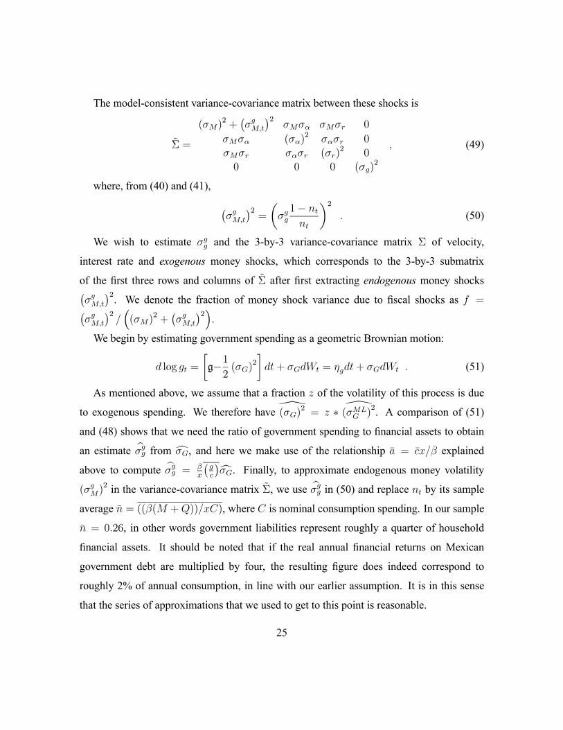
The model-consistent variance-covariance matrix between these shocks is
Σ =
(σM)2 +¡σgM,t
¢2σMσα σMσr 0
σMσα (σα)2 σασr 0
σMσr σασr (σr)2 0
0 0 0 (σg)2
, (49)
where, from (40) and (41), ¡σgM,t
¢2=
µσgg
1− ntnt
¶2
. (50)
We wish to estimate σgg and the 3-by-3 variance-covariance matrix Σ of velocity,
interest rate and exogenous money shocks, which corresponds to the 3-by-3 submatrix
of the first three rows and columns of Σ after first extracting endogenous money shocks¡σgM,t
¢2. We denote the fraction of money shock variance due to fiscal shocks as f =¡σgM,t
¢2/³(σM)2 +
¡σgM,t
¢2´.
We begin by estimating government spending as a geometric Brownian motion:
d log gt =
∙g−1
2(σG)2
¸dt + σGdWt = ηgdt + σGdWt . (51)
As mentioned above, we assume that a fraction z of the volatility of this process is due
to exogenous spending. We therefore have \(σG)2 = z ∗ \(σMLG )
2. A comparison of (51)
and (48) shows that we need the ratio of government spending to financial assets to obtain
an estimate bσgg from cσG, and here we make use of the relationship a = cx/β explained
above to compute bσgg = βx
¡gc
¢cσG. Finally, to approximate endogenous money volatility
(σgM)2 in the variance-covariance matrix Σ, we use bσgg in (50) and replace nt by its sample
average n = ((β(M + Q))/xC), where C is nominal consumption spending. In our sample
n = 0.26, in other words government liabilities represent roughly a quarter of household
financial assets. It should be noted that if the real annual financial returns on Mexican
government debt are multiplied by four, the resulting figure does indeed correspond to
roughly 2% of annual consumption, in line with our earlier assumption. It is in this sense
that the series of approximations that we used to get to this point is reasonable.
25

It is straightforward to estimate the drifts and variance-covariance matrix of M , α and rb,
again by maximum-likelihood. After subtracting our approximation of (σgM)2 from the first
cell of the variance-covariance matrix, we are left with nine entries can be used to separately
identify, including their signs, the nine diffusion processes σM , σα and σr. In doing so
we impose identifying restrictions, namely that real interest rates are completely exogenous
σMr = σαr = 0, and that the money supply responds instantaneously to velocity shocks but
not vice versa σMα = 0. Finally the estimated diffusions, from (45) and (46), can be used to
recover the drift processes µ and ν, while r can be estimated directly.
The results of our estimations and approximations are as follows: f = 0.5208, µ =
0.0773, ν = −0.0178, r = 0.0227, σgg = 0.0083, σMM = 0.0220, σαM = −0.0009,
σrM = 0.0025, σαα = 0.0294, σrα = −0.0059, σrr = −0.0186.
These results can be used to compute a baseline economy. To do so we also need to fix
velocity at its sample average α = 34.4 and the initial nominal exchange rate at its sample
average E = 9.35. This can then be used to compute the key initial quantities a, M and Q.
3.2 Monetary Policy
Monetary policy consists of an inflation target and balance sheet operations.16 It is
straightforward that the main tool for achieving an inflation target in the current flexible price
model is a target path µt∞t=0 for money. We will simply hold µ constant at its estimated
value for Mexico. The main subject of this paper is balance sheet operations, of which we can
distinguish three types. An unsterilized foreign exchange intervention is a sale or purchase of
foreign exchange reserves h in exchange for domestic money M . An open market operation
is a sale or purchase of domestic currency bonds Q in exchange for domestic moneyM . Such
operations can be used to ’sterilize’ the effect of an unsterilized intervention on the money
stock. A fully sterilized foreign exchange intervention is therefore a sale or purchase of
16 For simplicity, and because the relationship Pt = Et holds, we will conduct our discussionin terms of inflation and the price level instead of exchange rate depreciation and the nominal exchange rate.
26

domestic currency bonds Q in exchange for foreign currency bonds h, holding M constant.
We analyze the effect of balance sheet operations on equilibrium quantities using the
system of equations (37) - (44), holding constant αt = α Because full government
compensation for initial exchange rate jumps (18) is assumed, at is always constant on
impact at = a. The nine panels in Figure 2 show, going from the left to the middle
of each panel, the effect of a doubling of the nominal money supply through a foreign
exchange purchase. Going from the middle to the right, they show how the economy reacts
if this expansion of the money supply is reversed through a domestic open market operation
(OMO), specifically a sale of domestic currency bonds against money.
The foreign exchange intervention could be occasioned, for example, by the central bank
accommodating, on a one-off basis, a large capital inflow. But the effect would of course
be highly inflationary, causing a doubling of the price level. This in turn would negatively
affect the real value of domestic bonds and therefore the overall share of domestic assets in
agents’ portfolios. The government’s domestic liabilities however provide a cushion against
fiscal shocks, and this operation therefore not only doubles the price level, it also doubles the
subsequent volatility of inflation. Because inflation volatility increases the ex-ante return of
holders of domestic assets, the equilibrium interest rate can then fall by around 0.5%. The
cost to the government of higher inflation volatility turns out to outweigh the interest savings,
so that the government has to raise net taxes. Note that consumption is barely affected by the
change in interest rates, principally because, for the Mexican data set we used to calibrate
the baseline economy, velocity is extremely high. This may not be true for other countries,
and a significantly lower interest rate could then clearly stimulate consumption.
The open market operation completely sterilizes the foreign exchange intervention, so
that the exchange rate is driven back to its initial value. But importantly, other variables
do not return to their baseline values. Most importantly, while real money balances
are unchanged after sterilization, the real quantity of outstanding domestic liabilities has
increased significantly, thereby lowering inflation volatility, increasing interest rates, and
27

lowering the required tax rate to balance the government budget. Sterilized intervention
therefore has significant real effects, and as stated above with a lower velocity those effects
would also include lower consumption.
The following Figures 3-5 illustrate the effects of sterilized intervention over a broader
range of sterilized interventions. Figure 3 shows the Mexican baseline case. This time we
show the domestic asset share nt in % along the horizontal axis. The first panel shows
the relationship between the stock of domestic currency government securities Qt and nt.
Issuing more nominal debt increases the real debt stock given that full sterilization keeps the
nominal money stock constant. As the domestic debt share rises from 10% to 60%, fiscally
induced inflation volatility σgE,t falls from 1% in annual interest rate equivalent terms to near
zero, because more debt absorbs fiscal shocks through smaller price level movements. This
lowers overall inflation volatility by the same amount, because inflation volatility originating
from the three non-fiscal shocks is constant.17 As investors benefit from inflation volatility,
the equilibrium nominal interest rate has to rise. That rise is however very nonlinear, because
most of the effects of lower inflation volatility happen at lower levels of debt. From around
a 30% debt share onwards, further expansions of the nominal debt stock have quite modest
effects on inflation volatility and interest rates. Note that a higher interest rate also has
a secondary effect on mean inflation, but this is very minor compared to the effect of the
nominal anchor µt. Finally, as we saw above, a higher debt stock allows the government to
lower the mean tax rate, because the negative effect of higher interest rates on the budget is
more than offset by the beneficial effect of less volatile inflation.
Combining the above results, it is also clear that the effect of a given contraction of the
money supply depends on the market through which that contraction is implemented. The
effects on interest rates are larger if done through the domestic bond rather than the foreign
exchange market, because under open market operations the portfolio share nt expands not
just due to a drop in the price level but also due to an expansion of the domestic nominal17 It is also significantly smaller at low levels of debt issuance.
28

bond stock. This requires an even lower interest rate to establish portfolio balance.
Figures 4 and 5 show how these results on the effects of sterilized intervention depend
on the volatility of exogenous fiscal shocks, leaving all other parameters of the model
unchanged. Figure 4 shows that, when the fiscal shock diffusion σgg is reduced from 0.0083 to
0.002, balance sheet operations over the same range of Q as those reported in Figure 3 have
almost no effect on inflation volatility and interest rates, while we see in Figure 5 that raising
σgg to 0.024 increases the range over which they are effective, and it increases the size of their
effect on interest rates. This may explain why empirical studies of sterilized intervention
have found very little evidence for their effect in industrialized countries. In such countries
the fiscal situation is generally much more robust, and fiscal dominance is much less of
a problem. At the same time, even if there was fiscal dominance, the ability of such
countries to issue substantial amounts of domestic currency denominated debt means that
the induced inflation volatility would be comparatively low. On the other hand, developing
countries routinely engage in sterilized intervention, especially when faced with volatile
capital inflows, and they have much more difficulty issuing substantial stocks of domestic
currency debt. In such countries sterilized intervention would be a second tool of monetary
policy that gives the central bank autonomy to set nominal interest rates independently of
the inflation target. The bottom line is that low outstanding stocks of domestic currency
debt combined with high fiscal volatility give rise to imperfect asset substitutability between
domestic and foreign currency debt, and that this is most likely to be observed in developing
countries.
29

4 CONCLUSION
We have studied a general equilibrium monetary portfolio choice model of a small
open economy with floating exchange rates and flexible prices. The model emphasizes the
importance of fiscal policies for the number of instruments available to monetary policy,
specifically for its ability to affect allocations and prices through balance sheet operations
such as sterilized intervention. Conventional results were shown to depend on a particular
assumption about fiscal policy, full lump-sum redistribution of stochastic seigniorage income
and an absence of exogenous fiscal spending shocks. When this assumption is relaxed, two
important results are obtained.
First, government balance sheet operations matters even if they do not affect the money
stock. Their primary effect is on the volatility of inflation, because a larger outstanding stock
of nominal government debt requires smaller price level movements to balance the budget
following an exogenous fiscal spending shock. The volatility of inflation in turn affects the
domestic nominal interest rate. Putting this differently, the central bank can set its domestic
interest rate and its inflation target independently to affect both the mean and the variance of
inflation.
Second, uncovered interest parity fails to hold. Large risk discounts are obtained when
a central bank’s nominal liabilities are small and the volatility of its fiscal shocks is high,
because fiscal shocks induce a high nominal exchange rate volatility that increases investors’
ex-ante return. On the other hand, risk premia become possible when a central bank issues
very large amounts of nominal liabilities, because of risk premia charged by international
lenders. Our paper has not focused on the latter aspect, but it has provided the analytical
apparatus for doing so.
A welfare analysis of different policy choices is currently beyond the scope of the paper,
but the outlines of the trade-off are clear. Up to some point the government can expand its
stock of nominal liabilities and achieve three objectives that, in more detailed models, are all
30
welfare improving. These are a reduction of mean inflation, a reduction of inflation volatility,
and a reduction of taxes needed to balance the budget. It can be shown that required taxation
begins to increase once households have to start borrowing and paying a risk premium in
order to finance further holdings of domestic currency denominated liabilities. The point
at which this may occur for a specific country could be earlier than assumed in the present
model, but there will nevertheless be a broad range over which a government should be able
to increase its issue of nominal liabilities with very positive effects.
31

Appendix I Returns on AssetsThe return on real money balances is derived using Itô’s law to differentiate Mt/Et
holding Mt constant:
mtdrmt = Mtd
µ1
Et
¶=
−Mt
E2t
Et
£εtdt + σEdBt + σgE,tdWt
¤+
1
2
2Mt
E3t
E2t
£(σE)2 + (σgE,t)
2¤dt ,
which yields the return
drmt =¡−εt + (σE)2 + (σgE,t)
2¢dt− σEdBt − σgE,tdWt . (A.1)
The real return on the domestic bond is given by its nominal interest rate iqt , minus the
change in the international value of domestic money as in (A.1). We have
drqt =¡iqt − εt + (σE)2 + (σgE,t)
2¢dt− σEdBt − σgE,tdWt . (A.2)
The real return on internationally tradable assets is exogenous and given by (3), which is
repeated here for completeness.
drbt = rdt + σrdBt + γI(nmt + nqt − 1) . (A.3)
Appendix II The Value FunctionThis Appendix verifies the conjectured value function V (at, t) = e−βtJ(at, t) =
e−βtX[ln(at) + ln(Y (t;xt))] and derives closed form expressions for X and Y (t;xt).
Substitute the conjecture, the optimality condition (17), and the government policy rules
(22), (23) and (24) into the Bellman equation (14). Then cancel terms to get
βX ln(at) + βX ln(Y (t;xt))−XY (t;xt)
Y (t;xt)
= ln(at)− ln(X)− ln(1 +iqtαt
)
+Xhr − αtn
mt − γI (1− nmt − nqt )
2i
−X2
h(σr)
2 +¡σgg¢2i
,
32

where Y (t;xt) = ∂Y (t;xt)/∂t. Equating terms on ln(at) yields
X = β−1 . (B.1)
This implies the first-order conditions (28) and (29) shown in the paper. We are left with
a differential equation in Y (t;xt) as follows:
Y (t;xt)
Y (t;xt)= β ln(Y (t;xt))− β ln(β) + β ln(1 + (iqt/αt))−
µr − β
1 + (iqt/αt)
¶(B.2)
+1
2
³(σr)
2 +¡σgg¢2´
+ γI (nmt + nqt − φ)2 .
The equilibrium set of equations determining the evolution of the economy are presented
in the text as (38) - (41). As argued there, this system has unique bounded solutions for,
among others, (nmt + nqt ). This means that all terms on the right-hand side of (B.2) are, or
can be expressed uniquely in terms of, exogenous policy or shock variables xt, as conjectured
at the outset. Furthermore,
∂Y (t;xt)
Y (t;xt)|Y (t;xt)=0 = β > 0 . (B.3)
This implies that Y (t;xt) is saddle path stable for any given xt, and is therefore uniquely
determined for each t and xt. It is instructive to consider the value of Y (t;xt) under some
simplifying assumptions. Let αt = α ∀t, let iq be set such that r(1 + (iq/α)) = β and
such that I = 0. Then we have (E(dat))/dt = 0 and ct = rat. We obtain a steady state
value Y = r exp
µ³−1β
´µ(σr)
2
2+
(σgg)2
2
¶¶. In the absence of the final term, we would have
J(at, t;xt) = 1β
ln(ct). However, the actual utility value of at is lower because of risk to the
return on internationally tradable assets and risk to asset accumulation due to government
spending volatility.
Our approach has followed Duffie’s (1996, Ch. 9) discussion of optimal portfolio and
consumption choice in that we have focused mainly on necessary conditions. This is because
the existence of well-behaved solutions in a continuous-time setting is typically hard to prove
in general terms. We have adopted the alternative approach of conjecturing a solution and
33

then verifying it, and have found that our conjecture V (at, t) does solve the Hamilton-Jacobi-
Bellman equation and is therefore a logical candidate for the value function. In the process
of doing so we have also solved for the associated feedback controls (nq∗t , nm∗t ) and wealth
process a∗t . We now verify that V (at, t) and (nq∗t , nm∗t ) are indeed optimal.
Note first that our solutions solve the problem
supnmt,nqt
ln(αtnmt at − y) + DJ(at, t) = 0 , (B.4)
where
DJ(at, t) = Ja(at, t)g(at, nmt, nq
t) +
1
2Jaa(at, t)
£h(at, n
mt, nq
t)¤2 − βJ(at, t) + J(at, t) .
(B.5)
The functions g(., ., .) and h(., ., .) derive from the equilibrium evolution of wealth at given
the conjectured form of the value function V (at, t) and given the associated feedback
controls (nq∗t , nm∗t ). Let σa = [σr
¡−σgg
¢] and Zt = [Bt Wt]
0. Then we have
dat = g(at, nmt, nq
t)dt + h(at, n
mt, nq
t)dZt ,
where
g(at, nmt, nq
t) = rat + y − αtn
mt at ,
h(at, nmt, nq
t) = atσa ,
and where in line with our previous notation£h(at, n
mt, nq
t)¤2
= a2t
h(σr)
2 +¡σgg¢2i.
Now let (nqt , nmt ) be an arbitrary admissible control for initial wealth a0 and let at be the
associated wealth process. By Itô’s formula, the stochastic integral for the evolution of the
quantity e−βtJ(at, t) can be written as
e−βtJ(at, t) = J(a0, 0) +
Z t
0
e−βsDJ(as, s)ds +
Z t
0
e−βsψsdBs , (B.6)
where ψt = Ja(at, t)h(at, nmt, nq
t) .
We proceed to take limits and expectations of this equation. We show first that
E³R t
0e−βsψsdBs
´= 0. To do so we need to demonstrate that
R t0e−βsψsdBs is a martingale,
34

which requires that e−βsψs satisfies EhR t
0
¡e−βsψs
¢2dsi<∞ , t > 0. In our case, we have
simply that ψt = σa/β, where β > 0. The condition is therefore satisfied, and we have that
limt→∞
E0
©e−βtJ(at, t)
ª= lim
t→∞E0
½J(a0, 0) +
Z t
0
e−βsDJ(as, s)ds
¾(B.6’)
= J(a0, 0) +
Z ∞
0
e−βsDJ(as, s)ds .
The transversality condition (15) can easily be verified because both wealth at and the
term Y (t;xt) at most grow at an exponential rate. The left-hand side of (B.6’) is therefore
zero. Because the chosen control is arbitrary, (B.4) implies that
−DJ(at, t) = ln(αtnmt at − y) ,
and therefore
J(a0, 0) =Z ∞
0
e−βs ln(αsnms as − y)ds . (B.7)
On the other hand, when we do the same calculation for our feedback controls (nq∗t , nm∗t )
we arrive at (B.7) but with = replaced by an equality sign:
J(a0, 0) =
Z ∞
0
e−βs ln(αsnm∗s a∗s − y)ds . (B.8)
We therefore conclude that J(a0, 0) dominates the value obtained from any other
admissible control process, and that the controls (nq∗t , nm∗t ) are indeed optimal.
Appendix III DataQuarterly data from the first quarter of 1996 through the second quarter of 2004 are
used. We use an interpolated series of annual population figures obtained from International
Financial Statistics (IFS) to convert aggregate to per capita series, and we use Peso-dollar
exchange rate data obtained from Banco de Mexico to convert nominal to real series.
Because the velocity series is a ratio of a stock to a flow, we used as our stock data series
the midpoint of each quarter instead of the endpoint. For consistency we did so all series,
including base money. The series for nominal base money is from Banco de Mexico, and is
converted to per capita terms. The velocity series is the ratio of nominal domestic absorption
35

(from IFS) to the stock of base money, where quarterly absorption is multiplied by four
to obtain an annual series. Real interest rates are gross annualized US treasury bill rates
divided by gross annualized one-quarter ahead US CPI inflation (from IFS).18 Government
spending is computed as the sum of government consumption and government investment
from national accounts data available at Banco de Mexico, and put on a real per capita
basis by divided by the exchange rate and population. Finally, we need to compute the
sample average portfolio share of Mexican government liabilities. To do so we obtain data
for nominal outstanding stocks of base money M and government debt Q from Banco de
Mexico. Nearly all Mexican government debt is denominated in local currency.
18 We have also worked with the log difference of the CPI-deflated S&P500 index. The mainresults of the paper do not change in that case.
36

ReferencesAït-Sahalia, Y. (2002), ’Maximum Likelihood Estimation of Discretely Sampled Diffusions:A Closed-Form Approximation Approach’, Econometrica, 70(1), 223-262.Aizenman, J. (1989), ’Country Risk, Incomplete Information and Taxes on InternationalBorrowing’, Economic Journal, 99, 147-161.Backus, D.K. and Kehoe, P.J. (1989), ’On the Denomination of Government Debt - A Cri-tique of the Portfolio Balance Approach’, Journal of Monetary Economics, 23, 359-376.Bakshi, G.S. and Chen, Z. (1997), ’Equilibrium Valuation of Foreign Exchange Claims’,Journal of Finance, 52, 799-826.Bansal, R. and Dahlquist, M. (2000), ’The Forward Premium Puzzle: Different Tales fromDeveloped and Emerging Economies’, Journal of International Economics, 51(1), 115-144.Branson, W.H. and Henderson, D.W. (1985), ’The Specification and Influence of Asset Mar-kets’, Ch. 15 in: Handbook of International Economics, vol. 2.Cambbell, J.Y., Lo, A.W. and MacKinlay, A.C. (1997), The Econometrics of FinancialMarkets, Princeton University Press, Princeton, New Jersey.Canzoneri, M.B., Cumby, R.E. and Diba, B.T. (2004),’Is the Price Level Determined by theNeeds of Fiscal Solvency?’, American Economic Review (forthcoming).Chamley, C. and Ptolemarchakis, H. (1984), ’Assets, General Equilibrium, and the Neutral-ity of Money’, Review of Economic Studies, 51, 129-138.Chow, G.C. (1979), ’Optimum Control of Stochastic Differential Equation Systems’, Jour-nal of Economic Dynamics and Control, 1, 143-175.Cox, J.C., Ingersoll, J.E. and Ross, S.A. (1985), ’An Intertemporal General EquilibriumModel of Asset Prices’, Econometrica, 53(2), 363-384.Duffie, D. (1996), Dynamic Asset Pricing Theory, 2nd edition, Princeton University Press,Princeton, NJ.Dumas, B. and Uppal, R. (2000), “Global Diversification, Growth and Welfare with Imper-fectly Integrated Markets for Goods”, Manuscript, INSEAD and MIT.Eaton, J. and Gersovitz, M. (1981), “Debt with Potential Repudiation: Theoretical and Em-pirical Analysis”, Review of Economic Studies, 48, 289-309.Edison, H.J. (1993), ’The Effectiveness of Central Bank Intervention: A Survey of the Litera-ture since 1982’, Special Papers in International Economics No. 18., Princeton University,Princeton, NJ.
37

Devereux, M.B. and Engel, C. (1998), ’Fixed versus Floating Exchange Rates: How PriceSetting Affects the Optimal Choice of Exchange Rate Regime’, NBER Working Paper No.6867.Engel, C. (1992), ’On the Foreign Exchange Risk Premium in a General Equilibrium Model’,Journal of International Economics, 32, 305-319.Engel, C. (1999), ’On the Foreign Exchange Risk Premium in Sticky-Price General Equilib-rium Models’, NBER Working Paper No. 7067.Feenstra, R.C. (1986), ’Functional Equivalence between Liquidity Costs and the Utility ofMoney’, Journal of Monetary Economics, 17, 271-291.Fleming, W.H. and Rishel, R.W. (1975), Deterministic and Stochastic Optimal Control,Springer Verlag, New York, NY.Gavin, M. and Perotti, R. (1997), ’Fiscal Policy in Latin America’, (Manuscript, Inter-American Development Bank and Columbia University).Grinols, E.L. and Turnovsky, S.J. (1994), ’Exchange rate determination and asset prices in astochastic small open economy’, Journal of International Economics, 36, 75-97.Karatzas, I. and Shreve, S.E. (1991), Brownian Motion and Stochastic Calculus, 2ndedition, Springer Verlag, New York, NY.Kehoe, P.J. and Perri, F. (2001), ’International Business Cycles with Endogenous IncompleteMarkets’, Econometrica (forthcoming).Kletzer, K.M. and Wright, B.D. (2000), ’Sovereign Debt as Intertemporal Barter’, AmericanEconomic Review, 90(3), 621-639.Kumhof, M. and van Nieuwerburgh, S. (2002), ’A Fiscal Theory of the Currency Risk Pre-mium and of Sterilized Intervention’, IMF Working Paper WP/02/29.Lucas, Robert E. jr. (1982), ’Interest Rates and Currency Prices in a Two-Country World’,Journal of Monetary Economics, 10, 335-359.Lucas, Robert E. jr. (1990), ’Liquidity and Interest Rates’, Journal of Economic Theory,50, 237-264.Malliaris, A.G. and Brock, W.A. (1982), Stochastic Methods in Economics and Finance,1st edition, Advanced Textbooks in Economics, Volume 17, Elsevier, Amsterdam.Merton, R.C. (1969), ’Lifetime Portfolio Selection under Uncertainty: The Continuous-TimeCase’, The Review of Economics and Statistics, 51, 239-246.Merton, R.C. (1971), ’Optimum Consumption and Portfolio Rules in a Continuous-TimeModel’, Journal of Economic Theory, 3, 373-413.
38

Montiel, P.J. (1993), ’Capital Mobility in Developing Countries’, The World Bank WorkingPaper Series 1103.Obstfeld, M. (1982), ’The Capitalization of Income Streams and the Effects of Open-MarketPolicy under Fixed Exchange Rates’, Journal of Monetary Economics, 9, 87-98.Obstfeld, M. (1987), ’Peso Problems, Bubbles, and Risk in the Empirical Assessment ofExchange-Rate Behavior’, NBER Working Paper No. 2203.Obstfeld, M. and Rogoff, K. (1996), Foundations of International Macroeconomics, 1stedition, MIT Press, Cambridge, MA.Obstfeld, M. and Rogoff, K. (1998), ’Risk and Exchange Rates’, NBER Working PaperNo. 6694.Obstfeld, M. and Rogoff, K. (2000), ’New Directions for Stochastic Open Economy Mod-els’, Journal of International Economics, 50, 117-153.Sargent, T.J. and Smith, B.D. (1987), ’The Irrelevance of Government Foreign ExchangeOperations’, in: Helpman, E., Razin, A. and Sadka, E., eds., Economic Effects of theGovernment Budget, Cambridge, Mass. and London: MIT Press.Sargent, T.J. and Smith, B.D. (1988), ’Irrelevance of Open Market Operations in SomeEconomies with Government Currency Being Dominated in Rate of Return’, AmericanEconomic Review, 77(1), 78-92.Stulz, R.M. (1983), ’The Demand for Foreign Bonds’, Journal of International Economics,15, 225-238.Stulz, R.M. (1984), ’Currency Preferences, Purchasing Power Risks, and the Determinationof Exchange Rates in an Optimizing Model’, Journal of Money, Credit and Banking,16(3), 302-316.Stulz, R.M. (1987), ’An Equilibrium Model of Exchange Rate Determination and AssetPricing with Nontraded Goods and Imperfect Information’, Journal of Political Economy,95(5), 1024-1040.Stulz, R.M. (1988), ’Capital Mobility and the Current Account’, Journal of InternationalMoney and Finance, 7, 167-180.Uribe, M. (2001), ’A Fiscal Theory of Sovereign Risk’, (Manuscript, University of Pennsyl-vania).Wallace, N. (1981), ’A Modigliani-Miller Theorem for Open Market Operations’, AmericanEconomic Review, 71, 267-274.Zapatero, F. (1995), ’Equilibrium Asset Prices and Exchange Rates’, Journal of EconomicDynamics and Control, 19, 787-811.
39

0
2
4
6
8
10
12
14
16
18
20
Jan-96
May
-96
Sep-96
Jan-97
May
-97
Sep-97
Jan-98
May
-98
Sep-98
Jan-99
May
-99
Sep-99
Jan-00
May
-00
Sep-00
Jan-01
May
-01
Sep-01
Jan-02
May
-02
Sep-02
Jan-03
May
-03
Sep-03
Jan-04
May
-04
Sep-04
Figure 1: Foreign Holdings of Mexican Government Securities - % of Total (Source: Banco
de Mexico)
40

Initial Forex Intervention OMO
10
12
14
16
18
Nominal Exchange Rate
Initial Forex Intervention OMO
7.72
7.74
7.76
Inflation
Initial Forex Intervention OMO
1.0203
1.0204
1.0204
1.0205Consumption
Initial Forex Intervention OMO
8
10
12
14
16
Domestic Asset Share
Initial Forex Intervention OMO
0.6
0.8
1
1.2Inflation Volatility
Initial Forex Intervention OMO
−0.56
−0.54
−0.52
Required Tax Rate on Wealth
Initial Forex Intervention OMO
9
9.5
10
Interest Rates
Initial Forex Intervention OMO
0.4
0.6
0.8
1
sigmaeg.squared
0 0.2 0.4
0.15
0.2
0.25
0.3
Money
Velocity
Interest Rate
Price Level Diffusions x 10
Figure 2: Unsterilized Foreign Exchange Purchase and Open Market Sale
41

4.04 10 20 300
1
2
Nominal Debt and Money
4.04 10 20 307.7
7.75
7.8
7.85
Inflation
4.04 10 20 30
1.0203
1.0204
1.0204
1.0205
Consumption
4.04 10 20 306
7
8
9
10
Interest Rates
4.04 10 20 30
1
2
3
4
Inflation Volatility
4.04 10 20 30
−0.55
−0.5
−0.45
−0.4
−0.35
Required Tax Rate on Wealth
4.04 10 20 30
9.3
9.35
9.4
9.45Nominal Exchange Rate
4.04 10 20 30
1
2
3
4
sigmaeg.squared
4.04 10 20 30
0.15
0.2
0.25
0.3
Money
Velocity
Interest Rate
Exchange Rate Diffusions x 10
Figure 3: Sterilized Foreign Exchange Intervention - Baseline Case
42

4.04 10 20 300
1
2
Nominal Debt and Money
4.04 10 20 307.67
7.68
7.69
Inflation
4.04 10 20 30
1.0203
1.0204
1.0204
1.0205Consumption
4.04 10 20 309.6
9.7
9.8
9.9
Interest Rates
4.04 10 20 30
0.2
0.3
0.4Inflation Volatility
4.04 10 20 30−0.58
−0.57
−0.56
−0.55
Required Tax Rate on Wealth
4.04 10 20 30
9.3
9.35
9.4
9.45Nominal Exchange Rate
4.04 10 20 300
0.1
0.2
sigmaeg.squared
4.04 10 20 30
0.15
0.2
0.25
0.3
Money
Velocity
Interest Rate
Exchange Rate Diffusions x 10
Figure 4: Sterilized Foreign Exchange Intervention - Low Volatility of Fiscal Shocks
43

10.45 20 30 40 50
1
2
3
4
Nominal Debt and Money
10.45 20 30 40 507.8
7.9
8
8.1
8.2
Inflation
10.45 20 30 40 50
1.0203
1.0204
1.0204
1.0205
Consumption
10.45 20 30 40 50
6
7
8
9
10
Interest Rates
10.45 20 30 40 50
1
2
3
4
5
Inflation Volatility
10.45 20 30 40 50
−0.5
−0.45
−0.4
−0.35
−0.3
Required Tax Rate on Wealth
10.45 20 30 40 50
9.3
9.35
9.4
9.45Nominal Exchange Rate
10.45 20 30 40 50
1
2
3
4
5
sigmaeg.squared
10.45 20 30 40 50
0.15
0.2
0.25
0.3
Money
Velocity
Interest Rate
Exchange Rate Diffusions x 10
Figure 5: Sterilized Foreign Exchange Intervention - High Volatility of Fiscal Shocks
44