Cumulative Causation and EvolutionaryMicro-Founded Technical Change :A Growth Model with Integrated Economies∗

Patrick Llerena†

Andre Lorentz‡

Version 1.01 : May 2003

Abstract

We propose to develop in this paper an alternative approach tothe New Growth Theory to analyse growth rate divergence amongintegrated economies. The model presented here considers economicgrowth as a disequilibrium process. It introduces in a cumulative cau-sation framework, micro-founded process of technical change takinginto account elements rooted in evolutionary and Neo-Austrian liter-ature. We then attempt to open the ‘Kaldor-Verdoorn law black-box’using a micro-level modelling of industrial dynamics.

We use this framework to study the nature and sources of growthrate divergence, focusing on the effect of some macro-economic pa-rameters (income elasticities) and of some technological parameters(technological opportunities and absorptive capacities). If the resultsremain broadly in Kaldorian lines, this framework allows for moresubtle considerations of growth rate divergence.

∗Authors would like to thank M. Anoufriev, C. Castaldi, G. Fagiolo and R. Gabrielefor their precious comments on this work. The research has been supported by the EU,under the research programme “MACROTEC” (HPSE CT 1999 00014), and did especiallybenefit from the discussions and comments from Nick Von Tunzelmann (SPRU). All usualdisclaimers should nevertheless apply.

†Bureau d’Economie Theorique et Appliquee, Universite Louis Pasteur - Strasbourg,e-mail: pllerena@cournot.u-strasbg.fr

‡Laboratorio di Economia e Management, Scuola Superiore Sant’Anna di Studi Uni-versitari e di Perfezionamento - Pisa and Bureau d’Economie Theorique et Appliquee,Universite Louis Pasteur - Strasbourg, e-mail: alorenz@sssup.it

1

1 Introduction.

The literature on economic growth is dominated since the 90s by the devel-opments of the New Growth Theory (NGT), also called “Endogenous growththeory”. It is at least a good indicator of the relevance of two propositions :

- to explain why economies growth is again a relevant and still an openquestion in economics;

- the factors of growth should be “endogenous” to be acceptable; thateconomist should go beyond the simplified version of the Solow canon-ical model, with exogenous technical changes.

But at the same time, this literature did hide a long tradition of researchwhich could certainly give some alternative explanations to the persistenceof phenomena such as growth rate divergence among countries or regions.Among these potential alternatives there are at least three which are worthmentioning in the context of our paper: the Kaldorian approaches of a cumu-lative causation, the evolutionary perspectives of diversity and selection andthe Austrian view of the decision sequences and path dependency. Even if itis usually considered that the alternative approaches are too heterogeneousto be built into an integrated and coherent framework; they have at leastsome common features which could justify a comprehensive complementar-ity. Contrary to the NGT, all three approaches economise in terms of degreeof rationality of economic agents, escape from technologies being dealt wihtas information , and introduce innovation as a process of knowledge creation,and finally consider that ‘history matters’ i.e. the focus should be rather inthe ‘out of equilibrium’ processes than on the equilibrium characteristics andexistence.

The purpose of this paper is not to propose a ‘re-constructed’ and ‘in-tegrated’ alternative theory of growth, but to build a simple model, inte-grating some of the main features of these alternative theories in order toshow their complementarity in explaining some classical ‘stylised phenom-ena’. Our focus will be in this paper the growth rate divergence amongintegrated economies.

The main aspect of Kaldorian approaches (Kaldor (1972, 1981) ; Dixonand Thirlwall (1975); Verspagen (2002)) is essentially based on two principles:A demand-driven growth and a cumulative causation. In this framework,Kaldor’s explanation of growth rate is the result of two “interrelated mecha-nisms” : First output growth is driven by the growth of aggregate demand,so that growth and technological progress are demand-driven processes. In

2

Kaldor’s mind this aggregate demand factor driving growth is concretely rep-resented by the growth of exports that are driven by the country’s degreeof international competitiveness. Second, productivity is a “by-product ofoutput”; this is due to the existence of dynamic increasing returns throughthe Verdoorn law and the mechanisms underlying it. The interrelation be-tween these two mechanisms can be described as follows. The rule for pricesis a mark-up over unit labour cost. The growth of productivity based on thegrowth of output would reduce this unit labour cost, then prices, and thus in-crease the country’s competitiveness. This increasing competitiveness wouldlead to increasing exports, themselves leading to a higher growth rate. Thusfor a given initial competitiveness advantage, growth rates will tend, throughthe circular and cumulative mechanisms, to be maintained or increased overtime, by themselves. This implies also that initial conditions strongly dic-tate the growth process, providing for virtuous cumulative mechanisms (asdescribed previously) rather than a vicious one where growth could never beself-sustained and so cumulative processes could never start.

The major mechanisms driving the Kaldorian cumulative growth pro-cess can be summarised as follows: the Verdoorn law allows self-sustainedgrowth, dynamic increasing returns allow cumulativeness of the growth pro-cess, and finally initial conditions define this process as a path-dependentprocess, where initial competitiveness differences tend to increase rather thandecrease.

One of the main drawbacks of the approach is the “Kaldor-Verdoorn blackbox”. Our paper is to substitute it with a micro-founded technical change,using a evolutionary model of industrial dynamics a la Nelson and Winter(1982). The main task is here to model the innovation process (through R&Dexpenditure by firms, innovation and integration into new investments), inorder to endongenise the evolution of productivity and so to close the modelwith a micro-founded alternative to the Kaldor-Verdoorn law.

Finally we have some Austrian flavour in our model, because we explicitlyconstraint the decision process at the firm level to a given sequence: invest-ment and R&D expenditure are financially constrained by previous profits.The liquidity constraint is essential as a device to structure both the ongoingprocesses: selection and innovation.

Only few attempts exist in the literature to merge these approaches, themain one being by Verspagen (1993, 2002). Our contribution is principally toadd a fully specified model, as a first step for further developments. In partic-ular we wish to differentiate the impact of macro diversity from technologicaldiversity among countries in terms of divergence-convergence of growth rate.

3

The main point of our model is that, even if it is a combination of differ-ent approaches, is to preserve one of their major feature : unlike new growththeories, it never assumes full employment, but above all never considers ageneral equilibrium framework for analysing growth, so it never assumes theexistence of a natural rate of growth along a given balanced growth path.The growth process is cumulative in this analysis because “growth createsthe necessary resources for growth itself”1. This cumulative process allowsan endogeneity of growth through growth itself as a self-reinforcing process.

The next section is devoted to a presentation of the model, followed, insection 3, by the development both of the main results and of their interpre-tations.

2 A model of cumulative causation growth

with evolutionary micro-founded industrial

dynamics.

In order to consider the co-evolution of these components, we assume that ag-gregate demand is defined at the macro-economic level, through the balanceof payment constraint. First, demand provides the necessary resources forfirms to finance their activities and development (through both R&D and in-vestments). Second, selection among firms takes place at the macro-economiclevel, as resulting from international competition. Firms located in a givencountry compete among themselves and with foreign firms on an integratedmarket2. Hence the macro-dynamics can be considered as a constraint onfirm micro-dynamics.

On the other hand technical change, a necessary engine for growth, isrooted in firms’ dynamics. The competitiveness of the entire economy relieson the firm’s ability to generate technological progress. In other words, firmscontains the essence of macro-dynamics.

As a consequence, micro and macro-dynamics are strongly interrelated.In this section we first present the macro-frame, then the micro-dynamics offirms.

1Leon-Ledesma (2000)2Assuming then neither trade limitations nor barriers to access foreign markets

4

2.1 Aggregate demand and the balance of paymentconstraint : the macro-frame.

We suppose that the economies under-consideration are part of an integratedsystem constrained by the balance of payment with fixed exchange rates ( ora common monetary system ). Moreover, assuming that the member coun-tries of the integrated system external debt with other members is restricted3.Given the monetary integration, the balance of payment adjustments throughmonetary mechanisms (exchange rates) are excluded and the balance of pay-ment constraint corresponds then to a clearing of countries trade balance.In other words imports have to match exactly exports, for each integratedeconomy.

The macro-economic framework we develop here is directly rooted in theformal interpretation of Kaldor’s cumulative causation approach of economicgrowth. These formal representations can be found among others in Dixonand Thirlwall (1975), or more recently Amable (1992), Verspagen (1993) andLeon-Ledesma (2000).

Economic growth is driven by demand. Aggregate demand is a function ofan autonomous component, represented by external demand, i.e. countries’exports. For each economy, exports are given as a function of the income ofthe rest of the world and of the market share of the economy.

Formally exports for a given economy4 j can be computed as follows:

Xj,t = (Yw,t)αjzj,t (1)

where Yw,t represents the GDP of the rest of the world, computed as the sumof GDP levels of all foreign economies, zj,t represents the market share of theeconomy, on the international markets and αj income elasticity to exportsfor the rest of the world.

The market share of the economy is a function of the price competitivenessof the country. In other words if the first component of the export functionrepresents the income determinant of exports, the market share then repre-sents the price component of external demand. The economy’s market shareis given by the sum of the market shares of the domestic firms (denoted zi,j,t):

zj,t =∑

i

zi,j,t

3We assume here that no external debt among member countries is allowed4Note that the subscript j always reefers to an economy, while the subscript i refers to

a firm. We suppose that the model is composed of J economies, each of them counts Ifirms. Hence a variable with the subscripts “j, i” concerns the firm i based in the countryj.

5

Each firm’s market share is defined through a replicator dynamics5, a functionof a firm’s relative competitiveness. Hence the market share of each firm willbe computed as follows :

zi,j,t = zi,j,t−1

(1 + φ

(Ei,j,t

Et

− 1))

(2)

where zi,j,t represents the market share of firm i, pi,j,t the price of its product,Ei,j,t stands for firm i’s level of competitiveness:

Ei,j,t =1

pi,j,t

Et the average competitiveness on the international market, given by:

Et =∑j,i

zj,i,t−1Ej,i,t

The parameter φ ∈ [0; 1] represents the degree of reactivity of demand toprice competitiveness.

To complete the formal definition of the macro-economic framework, wehave to define the economy’s imports. They are basically defined followingexports’ scheme, as a function of the domestic economy income and of therest of the world’s market share. Formally imports will be represented asfollows:

Mj,t = (Yj,t)βj(1− zj,t) (3)

The parameter βj represents the income elasticity to import. Yj,t repre-sents the economy GDP equal to the sum of firms production.

The growth rate of exports and imports for each sector can be deducedfrom these previous expressions as :

xj,t = αjyw,t + ln(zj,t)− ln(zj,t−1) (4)

mj,t = βjyj,t + ln(1− zj,t)− ln(1− zj,t−1) (5)

Where xjt, mjt, yt and yw,t stand for the growth rates6 of the previouslydefined corresponding variables.

We assume that each economy has to satisfy the balance of paymentconstraint. In our model this corresponds to an equilibrated trade balance.

5For a comprehensive view on the use of the replicator dynamics in evolutionary eco-nomics see Metcalfe (1998)

6Approximated through difference in logarithms.

6

An economy j’s external expenditures have to match exactly its externalresources. In other words each economy is subject to an external financialconstraint. Formally, exports have to equal imports:

Mj,t = Xj,t

Dynamically, the growth rate of imports is constrained by the growth rateof exports:

mj,t = xj,t

The introduction of the balance of payment constraint allows us to expressthe GDP growth rate as function of the growth rate of GDP of the rest of theworld and of the growth rate of market share. GDP growth rate for countryj is computed as follows:

yj,t =αj

βj

yw,t +1

βj

[ln

(zj,t

zj,t−1

)− ln

(1− zj,t

1− zj,t−1

)](6)

The first component of the right end side of the equation captures infact Harrod’s trade multiplier. Hence GDP growth rate in our model will bedefined through the trade multiplier and through a second component linkedto the competitiveness of the economy. This second component is rooted infirms behaviours and characteristics. Hence, we can distinguish explicitly thegrowth effect linked to the trade multiplier and the one emerging from firmdynamics.

We can deduce from the expression for GDP growth rate the GDP levelat time t. It equals the domestic aggregated demand. GDP is given by:

Yj,t = Yj,t−1

(Yw,t

Yw,t−1

)αjβj

(zj,t

zj,t−1

1− zj,t−1

1− zj,t

) 1βj

(7)

This expression also represents the gross production of all firms at timet. In our model, the time dimension allows aggregate supply to match en-tirely aggregate demand. We do not consider here explicitly the process ofcoordination of demand and supply in the market for goods.

Aggregate (economy wide) demand is then distributed among the firms inthe economy given their market shares on the integrated markets. This firstcomponent then constitutes the first macro-economic constraint the firmshave to face.

The second macro-economic constraint imposed on firms concerns thelabour market. Wages are in fact set at the macro-economic level. We assumehere that wages are strictly correlated to the average labour productivity in

7

the economy. We suppose here that labour supply is perfectly elastic tofirms labour demand : only productivity is considered in the process of wagedetermination.

Wages are set at period t for the next period, given the average labourproductivity in the economy at period t. As we will see below, firms produceat time t with a technology developed during the previous period, throughthe exploitation of the outcome of R&D activity. Hence wages used in periodt+1 and bargained in t are indexed on the productivity levels resulting fromthe technologies developed in t − 1. In other words wages will be set asfollows:

wj,t = wj,t−1

(Aj,t

Aj,t−1

)(8)

where Aj,t−1 represents the average labour productivity level of the economyj at time t. Given the average labour productivity as follows, given that theproductivity level at time t for each firm depends on the technology developedat time t− 1, represented by Ai,j,t−1:

Aj,t =

∑i zi,j,tAi,j,t−1∑

i zi,j,t

This second macro-economic constraint implies that at the firm level compet-itiveness will increase at time t as a function of the difference in productivitygrowth rate at time t−1 with respect to the average increase in productivityof the economy at time t− 2. It explains why the competitiveness of the en-tire economy will increase at time t as a function of the difference in averageproductivity growth rate at time t− 1 with its growth rate at time t− 2.

2.2 Evolutionary micro-foundations of technical change.

This second level of the model concerns firms and industrial dynamics. Weexplain here firms’ behaviour and characteristics. This part is largely inspiredby evolutionary literature on the modelling of industrial dynamics.7 Weassume here that firms are heterogeneous in their characteristics, i.e. in termsof productivity level, and in their investment behaviours in terms of R&Dand capital goods. Moreover, firms mutate, by learning about the productionprocess, improving their productivity, and by learning about their decisions,adapting the latter to their situation compared to their competitors. Hencefirms are bounded rational agents applying adaptive behaviour.

7See Kwasnicki (2001) for a comprehensive survey of evolutionary models of industrialdynamics, Silverberg and Verspagen (1995) for a comprehensive survey of evolutionarygrowth models based on “industrial dynamics”.

8

Firms will have two distinct but complementary roles in our model. Firstthey will produce the necessary resources to sustain economic growth, by re-sponding to the demand needs. Second they will increase the competitivenessof the economy by trying to improve their productivity level to survive theselection process. This second process will be broken down into two stages:

- Exploration or R&D. Firms first search for new production facilities,through innovation or adaptation of existing production facilities. Theoutcome of the R&D process is uncertain, and defines efficiency (interms of productivity) of the new generation of capital goods.

- Exploitation of R&D outcome. This second stage requires that firmsinvest to incorporate the outcome of research in the production process.This second stage is financed by profits, and then directly subject tothe success of previous investments.

More formally firms are modelled below.

Firms’ production processes are represented by Leontiev production func-tions with labour as a unique production factor. Capital enters indirectly inthe production function by influencing labour productivity. Investment inthe different generations of capital goods will increase labour productivity.The production function will then be represented as follows :

Yi,j,t = Ai,j,t−1Lpi,j,t (9)

where Yi,j,t is the output of firm i, producing in country j at time t. Ai,j,t−1

represents labour productivity and Lpi,j,t the labour force employed in the

production process. The output is constrained by the demand directed atthe firms and defined at the macro-economic level. The level of productionof each firm is computed as a share of GDP given by their relative marketshares such as:

Yi,j,t =zi,j,t∑i zi,j,t

Yj,t

Labour productivity is a function of the firms’ accumulated generationsof capital goods through investment:

Ai,j,t =Ii,j,tai,j,t−1∑t

τ=1 Ii,j,τ+

∑t−1τ=1 Ii,j,τ∑tτ=1 Ii,j,τ

Ai,j,t−1(1− δ) (10)

where ai,j,t−1 represents the labour productivity embodied in the capital gooddeveloped by i during period t− 1. The parameter δ represents the depreci-ation rate of capital goods. Ii,j,t represents the level of investment in capitalgoods of the firm. This component will be explained later.

9

Firms set prices through a mark-up process. This mark-up is appliedto the production costs (i.e. labour cost). To simplify the model, labourcosts linked to R&D activity are financed by profits. Thus prices can berepresented as follows:

pi,j,t = (1 + µj)wj,t−1

Ai,j,t−1

(11)

where pi,j,t represents the price set by firm i at time t, µj the mark-up coef-ficient and wj,t−1 the nominal wage set at the macro level as defined above.It should be noted that we assume here that the mark-up coefficients arefixed for each firms in a given economy. First this insures that the share ofprofits in GDP is constant over time, which corresponds to one of Kaldor’sstylised facts. Second, it does not really affect the results in terms of macro-dynamics of the economy, as shown by Dosi et al (1994) that consider themark-up coefficient as an endogenous variable. This can be explained bythe fact that a drastic reduction in the mark-up coefficient to increase thecompetitiveness of the firm, implies as well a drastic reduction in the profitsand thus in resources that can be used to finance R&D and then reducespotential productivity increases of the firm.

The firm’s profit level will then be computed as follows:

Πi,j,t = µjwj,t−1

Ai,j,t−1

Yi,j,t (12)

In the model profits constitutes the only financial resource for firms’ invest-ments.

To improve their competitiveness and thus gain some market shares firmshave to improve their production processes (i.e. to increase labour produc-tivity). The process of technical improvement can be divided into two dis-tinct phases. Firms explore new technological possibilities, through localsearch (innovation) and/or by capturing external technological possibilities(through spill-overs). This process leads to a production design (or capitalgood design) that can be exploited by firms in their production process. Thesecond stage consists then in the exploitation of the design by incorporatingit as a new generation of capital goods. The exploitation process is relatedto investment in capital goods and the exploration is related to investmentsin research. Given the process of obsolescence of capital goods we assumepriority is given to investments exploiting already discovered technologicalopportunities. Formally the latter will be represented as explained below:Investment in capital goods is financed by the profits of the firm, using ashare ιijt of sales. This share is defined through a decision rule given below;

10

firms adapt their investment behaviours to their relative (to average) com-petitiveness, as a direct response to the selection mechanisms. The capitalgoods investment decision rule will be the following:

ιi,j,t =

{ιi,j,t−1 if Ei,j,t ≥ Et

ιi,j,t−1

(1 + ξ

(Et−Ei,j,t

Et

))otherwise

where the parameter ξ ∈ [0; 1] represents the degree of adaptation of thefirm decision rule to its relative competitiveness gap and Et the averagecompetitiveness. This formulation of the investment decision in capital goodsinduces some aggregate structural effects according to the number of firmslagging behind relatively to the average competitiveness.8

Investment is subject to a financial constraint. Hence, as investments arecompletely financed by profits, they cannot exceed the period’s profit level.Formally this constraint will be represented as follows:

Ii,j,t = min

{ιi,j,tYi,j,t ; µj

wj,t−1

Ai,j,t−1

Yi,j,t

}(13)

Investment in R&D is decided according to the following decision rule :Firms then adapt their R&D investments to their relative technological gap.These investments are a share ρi,j,t of their sales.

ρi,j,t =

{ρi,j,t−1 if Ai,j,t ≥ At

ρi,j,t−1

(1 + ψ

(At−Ai,j,t

At

))otherwise

withAt =

∑j,i

zi,j,t−1Ai,j,t−1

R&D investment will correspond to the hiring of workers assigned to theresearch activity :

Lri,j,t =

1

wj,t−1

min{Πi,j,t − Ii,j,t; ρi,j,tYi,j,t} (14)

The model takes into account the sequential nature of the decision processand the existence of a financial constraint linked to the success (or failure)of previous decisions. The investment decision sequence is such that a prior-ity is given to exploitation (investment in capital goods). Then explorationinvestment (R&D) depends on the remaining resources. Resources availablefor investment depend on firms’ profits and on the outcome of their previous

8see Gaffard (1978), p.73 and following.

11

decisions. This gives the “industrial dynamics” part of the model an addi-tional “Austrian flavour”9 to our Kaldorian and evolutionary approach.

The formalisation of the R&D process is explicitly inspired by evolution-ary modelling of technical change. Hence following Nelson and Winter (1982)we consider that the probability of success of the R&D activity will increase

with the ratioLr

i,j,t

Yi,j,t. The outcome of R&D is itself uncertain and can be

formally represented as follows:

ai,j,t = max{ai,j,t−1, ai,j,t} (15)

ai,j,t ∼ N(ai,j,t−1, σi,j,t) (16)

Hence, the potential increase in labour productivity embodied in the genera-tion of capital developed during the R&D process, is a random variable, themean of which equals the previous period value. The variance is a function ofthe spill-overs absorbed by the firm. The variance given by σi,j,t will formallybe defined as follows:

σi,j,t = σj + χj (at−1 − ai,j,t−1)

where the parameter σj, is constant and related to the technology used injth economy. It represents the range of technological opportunities. Thevariable at−1 represents the worldwide maximal value of labour productivityembodied in already discovered generation of capital, i.e. it represents thetechnological frontier at time t − 1. Thus at−1 − ai,j,t−1 will represent thedistance between firm’s technological level and the frontier level, in otherwords, the technological gap. And finally, the parameter χj defines absorp-tive capacity10.

3 Growth rate divergence among integrated

economies.

The model as developed in the previous section aims to consider the de-terminants of possible divergence in GDP growth rates among integratedeconomies. Traditionally, mainstream economics considers that the inte-gration of economies and openness to trade imply convergence due to thediffusion of knowledge and/or technologies.

9see Amendola and Gaffard (1998), p.126)10We consider here exogenous and fixed values for the absorptive capacities

12

For Neo-Schumpeterian evolutionary economics, growth rates divergencedepends on the balance between two effects :

- Innovation, heterogeneous among economies both in its timing and inthe outcome, that increases differences in GDP growth rates, and

- Imitation that reduces this difference.

Hence in this framework growth rate divergence directly depends on theaccessibility of technologies, innovation and imitation capabilities, and onthe decision processes linked to R&D investment.

For the Kaldorian approach growth rate divergence is structural depend-ing on both demand and technological parameters, and cumulative, due tothe emergence of vicious and virtuous circles.

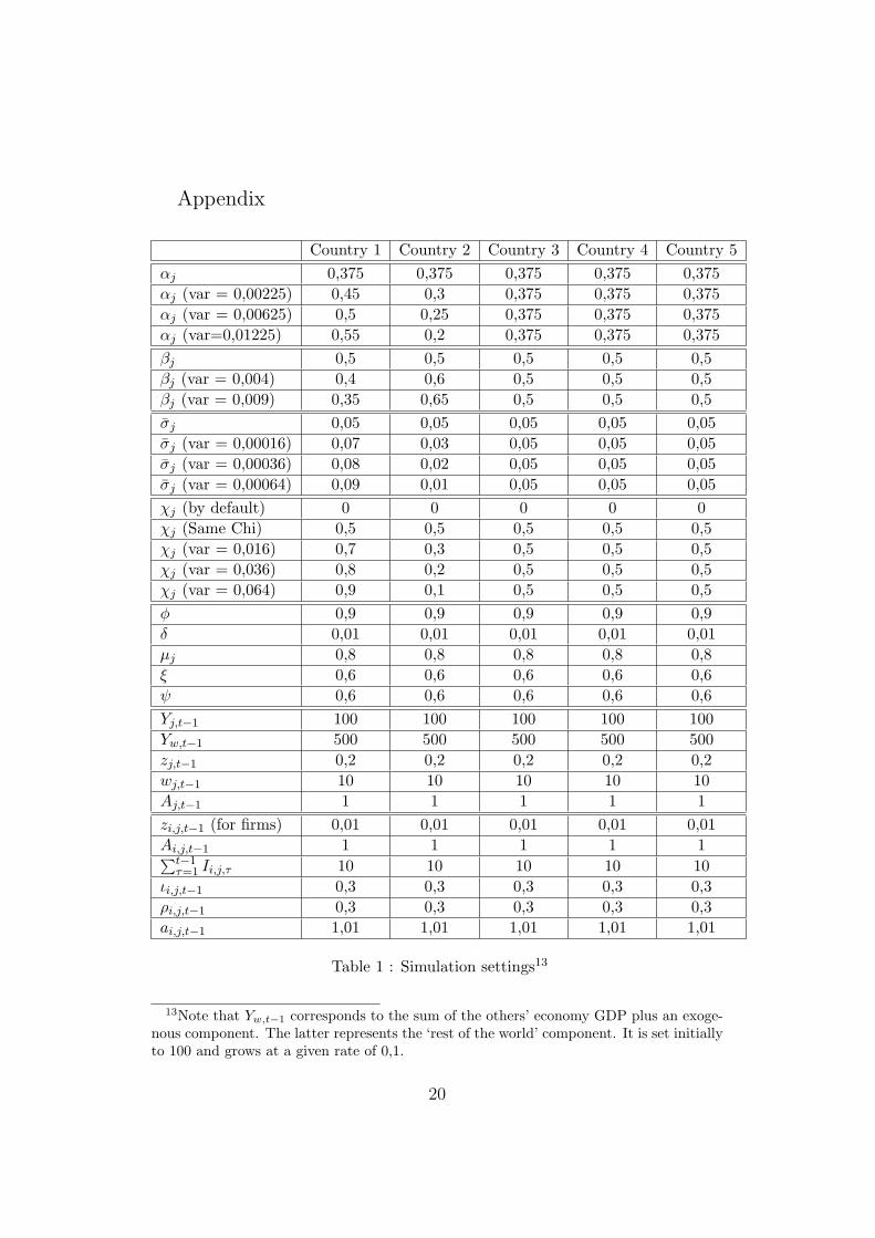
As for most of the models incorporating evolutionary features we need toresort to numerical simulations11. Simulations are set through the followingscheme. We consider 5 economies, each of which counts 20 firms. All thefirms of a given economy are equally defined (same initial conditions andparameters). The details of the parameters values used can be found inappendix.

We focus our analysis on the effect of four key parameters on growthrate divergence. Two of them concern the macro-economic constraint. Moreprecisely, we choose to concentrate on the effect of heterogeneous incomeelasticity of exports and imports, respectively αj and βj. The other twoconcern the process of technological change itself and are usually consideredin evolutionary literature. The first one concerns the range of technologicalopportunities represented by σj while the second concerns the absorptivecapacity χj.

To isolate the effect of each parameter we consider each of them sepa-rately, the other being then homogeneously set among economies. Moreover,when considering heterogeneity in the parameter setting, we use the follow-ing procedure : Over the five considered economies, three of them keep theinitial settings (also denoted reference setting) and the two remaining (de-noted Country 1 and Country 2) parameters are set in such a way that thefirst one gets the most favourable ones while the second gets the worth ones.Heterogeneous parameters are set so that the average value of the parametersamong economies remains unmodified. We only increase the variance.

One of the characteristic of the model is to generate two distinct types ofgrowth rate divergence:

11We used LSD (Laboratory for Simulation Development) environment to implementthe simulations. The source code for the model can be available on request to the authors

13

- A sustained growth rate divergence. In this case variance in growthrates stabilises itself over time. All economies continue to grow but atdifferent rates.

- A destructive growth rate divergence. In this case growth rate diver-gence increases over time. Divergence here leads to the collapse of somelagging economies coupled with the ongoing domination of others. Thissituation leads at the end to the survival of only one economy, the mostcompetitive one.

The key results of the simulations are detailed below.

3.1 Macro-constraint and growth rate divergence.

The first set of parameters concerns the macro-economic constraint due tothe trade balance restriction. We characterise the nature of the growth ratedivergence in this case.

Proposition 1 Increases in the heterogeneity of income elasticity of exportand imports respectively αj and βj increases the variance in growth ratesessentially by affecting the trade multiplier.

The effect of income elasticities (αj and βj) heterogeneity on growth ratedivergence is one of the main and maybe most obvious results one can thinkabout when considering a Kaldorian flavoured macro-economic framework.The increase in the divergence in growth rate due to this demand elasticitieseffect is in fact directly linked to the modifications induced on the trademultiplier in the definition of the GDP growth rate (see equation (8)).

Figure 1 and Figure 2 about here

Moreover, when considering the parameter βj, the latter does not only af-fect the trade multiplier but also modifies the weight of the market sharedynamics on GDP growth rates. There are then two opposite effects, onedirectly related to the trade multiplier. It increases the weight of a divergingprocess as when considering heterogeneous αj. The second effect is linkedto the increasing weight of a converging process, which is itself linked to themarket share dynamics, affected by technical change. When no spill-oversare absorbable, productivity growth rates (with homogenous parameters) areconvergent over time. This explains directly why the range of the variance ingrowth rates while modifying βj is lower then when modifying αj (see Figure1 and Figure 212).

12All the figures presented, unless otherwise mentioned, show the average values (ateach time step) over 50 simulation runs. Each simulation run lasts 500 time steps.

14

Proposition 2 Growth rate divergence generated by heterogeneity in de-mand parameters (αj and βj) generates sustained growth rate divergencewithout generating vicious circles.

As depicted in Figure 3 and Figure 4, the divergence in GDP growth ratesstands among times. The sustainability of this divergence without generatingvicious circles driving to the collapse of the least competitive economies differsfrom the usual Kaldorian results. It is principally due to the effect on thetrade multiplier, of the exports and imports elasticities, and the relativeneutrality of this effect on technological change. To generate a vicious circlegrowth rate divergence of GDP should directly affect competitiveness.

Figure 3 and Figure 4 about here

The differences in resources induced by the differences in aggregate demandgenerated through time by heterogeneous demand parameters are not suffi-cient to observe significant differences in technology levels (see Figure 5 andFigure 6).

Figure 5 and Figure 6 about here

In other words the macro-economic constraint is not sufficient to generatesignificant heterogeneity in technologies at the macro-level among economies.In particular this type of constraints does not generate destructive growthrate divergence usually induced by vicious circles.

3.2 Technology and growth rate divergence.

The second set of parameters considered in this analysis concerns the tech-nological characteristics of the economy. We concentrate on two of them,namely the range of technological opportunities (σj) and absorptive capaci-ties (χj), assuming that the economies are initially identically set (concern-ing the other parameters). It should be noted that heterogeneity in initialsettings of productivity levels does not generate significant or remarkableeffects on growth rate divergence among economies. Unless one considers ex-treme cases of heterogeneity, that will almost directly push the less favouredeconomies to enter a vicious circle.

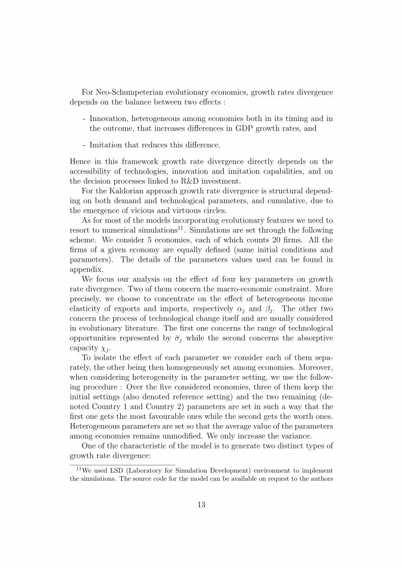
Proposition 3 Increasing heterogeneity in technological opportunity param-eter (σj), increases growth rate divergence among economies during a tran-sitory phase.

15

As depicted in Figure 7 and Figure 8 considering heterogeneous settingsfor the parameter defining the range of technological opportunity, increasesthe variance in GDP growth rates only during a transitory phase. Thesephases emerge when innovation is successful (which corresponds to a randomand rare event) and last for few time steps.

Figure 7 and Figure 8 about here

Moreover heterogeneity of technological opportunities also affects transitorilythe productivity levels (see Figure 9), even if the effect seems to last for longerperiods.

Figure 9 about here

The relative neutrality of uneven technological opportunities is directly dueto the macro-economic mechanisms of wage determination. The latter fol-lows the dynamics of productivity with a time lag. The gain in competitive-ness then depends mainly on the growth rate of productivity rather than onthe productivity levels themselves. Hence a higher increases in productivitylinked to wider technological opportunities will increase the GDP growth rateby increasing competitiveness until the complete adaptation of wages.

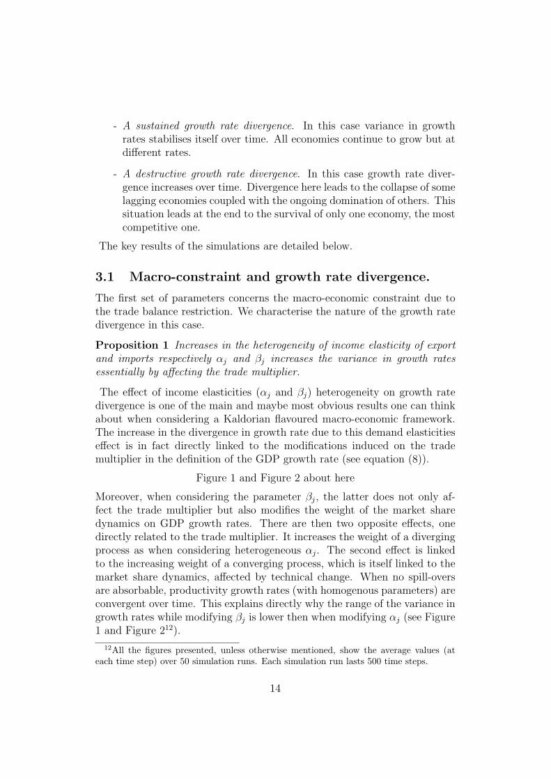
Proposition 4 Increasing access to spillovers (increasing χj) increases GDPgrowth rate divergence among economies.

Figure 10 about here

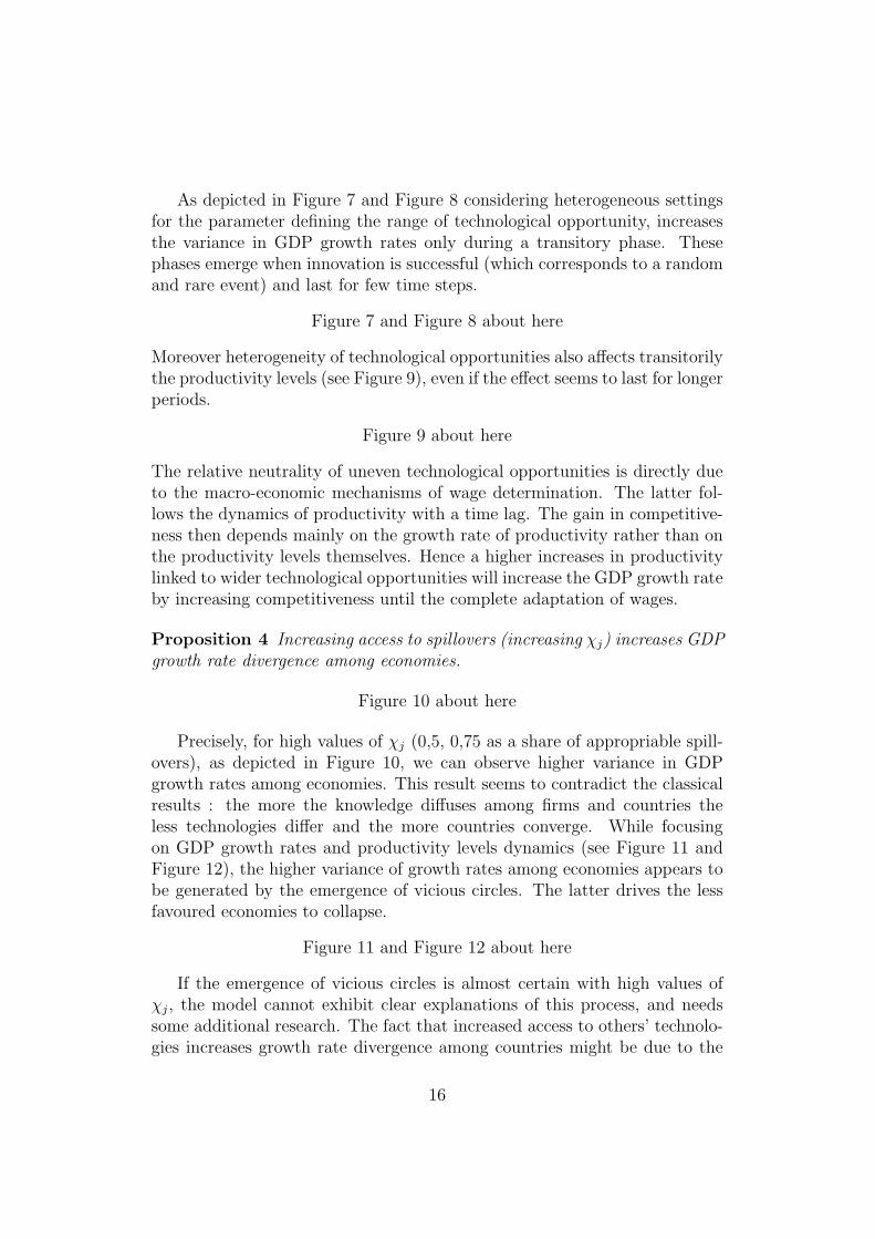
Precisely, for high values of χj (0,5, 0,75 as a share of appropriable spill-overs), as depicted in Figure 10, we can observe higher variance in GDPgrowth rates among economies. This result seems to contradict the classicalresults : the more the knowledge diffuses among firms and countries theless technologies differ and the more countries converge. While focusingon GDP growth rates and productivity levels dynamics (see Figure 11 andFigure 12), the higher variance of growth rates among economies appears tobe generated by the emergence of vicious circles. The latter drives the lessfavoured economies to collapse.

Figure 11 and Figure 12 about here

If the emergence of vicious circles is almost certain with high values ofχj, the model cannot exhibit clear explanations of this process, and needssome additional research. The fact that increased access to others’ technolo-gies increases growth rate divergence among countries might be due to the

16

additional effects of the macro-constraint combined with the absence of anintegrated outcomes of the R&D in the production process. Hence, the firmswhich gain higher market shares, might also benefit more from spillovers ;they have more resources to imitate (capture others technologies) and to ex-ploit others more efficient technologies. This puzzling result of the modelwill imply further analysis and development on absorption of spill-overs andimitation processes along the line of Llerena and Oltra (2002).

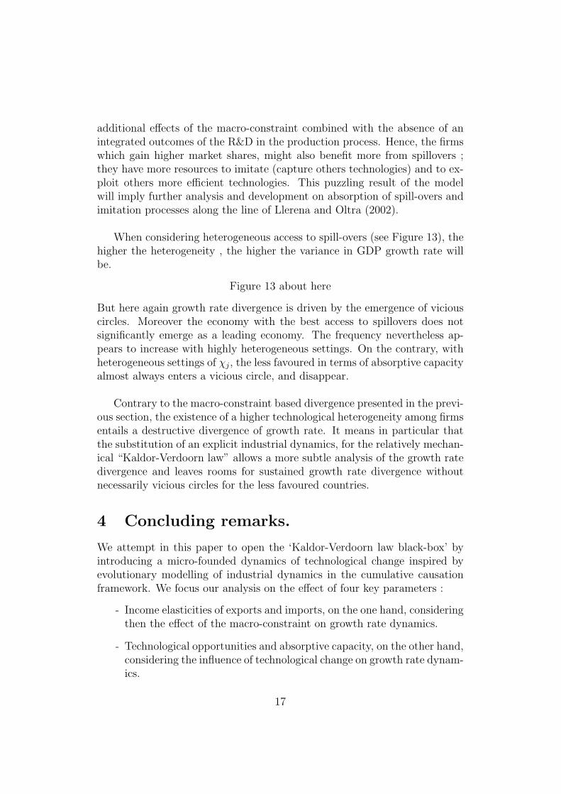
When considering heterogeneous access to spill-overs (see Figure 13), thehigher the heterogeneity , the higher the variance in GDP growth rate willbe.

Figure 13 about here

But here again growth rate divergence is driven by the emergence of viciouscircles. Moreover the economy with the best access to spillovers does notsignificantly emerge as a leading economy. The frequency nevertheless ap-pears to increase with highly heterogeneous settings. On the contrary, withheterogeneous settings of χj, the less favoured in terms of absorptive capacityalmost always enters a vicious circle, and disappear.

Contrary to the macro-constraint based divergence presented in the previ-ous section, the existence of a higher technological heterogeneity among firmsentails a destructive divergence of growth rate. It means in particular thatthe substitution of an explicit industrial dynamics, for the relatively mechan-ical “Kaldor-Verdoorn law” allows a more subtle analysis of the growth ratedivergence and leaves rooms for sustained growth rate divergence withoutnecessarily vicious circles for the less favoured countries.

4 Concluding remarks.

We attempt in this paper to open the ‘Kaldor-Verdoorn law black-box’ byintroducing a micro-founded dynamics of technological change inspired byevolutionary modelling of industrial dynamics in the cumulative causationframework. We focus our analysis on the effect of four key parameters :

- Income elasticities of exports and imports, on the one hand, consideringthen the effect of the macro-constraint on growth rate dynamics.

- Technological opportunities and absorptive capacity, on the other hand,considering the influence of technological change on growth rate dynam-ics.

17

The simulations results allow us to sort out two distinctive types of divergencein growth rates among economies.

On the one side, the model generates ‘sustained’ growth rate divergencewhile considering heterogeneous parameters for the macro-constraint. Thisresult seems to show that the macro-constraint might not directly influencecompetitiveness.

On the other, the model leads ‘destructive’ growth rate divergence, gen-erating vicious circles, if considering different settings of absorptive capacity.This result might be due to the reinforcement effect of the combination of themacro-constraint, the technical change sequentiality constraint by resources,and access to more efficient technologies, on randomly emerged competitiveadvantages. This last result opens the way for further development of theimitation process and absorptive capacity mechanisms.

Moreover, heterogeneity in technological opportunities seems to affecttransitorily growth rate divergence. Its effect on growth dynamics appearscounter-balanced by the wage determination process.

Hence, the introduction of evolutionary micro-foundations of technicalchange in a Kaldorian framework, allows for more subtle considerations inunderstanding growth rate divergence among integrated economies. How-ever, this model might constitute the starting point for further analysis.Hence, the way technical change is considered remains sketchy, and somemechanisms such as imitation, diffusion of technologies and its access forfirms might be reconsidered.

Finally, another aspect of Kaldorian literature concerns specialisationpatterns and their effect on growth dynamics. This concern, due to theone-sector specification of the model, is not considered here and might bethe object of further studies.

References

[1] B. Amable. Effets d’ Apprentissage, Competitivite Hors-prix et Crois-sance Cumulative. Economie Appliquee, 1992.

[2] M. Amendola and J.L. Gaffard. Out of Equilibrium. Clarendon Press,Oxford, 1998.

[3] J.S.L. Mc Combie and A.P. Thirlwall. Economic Growth and the Balanceof Payments Constraint. MacMillan Press, 1994.

[4] R. Dixon and A.P. Thirlwall. A Model of Regional Growth-rate Differ-ences on Kaldorian Lines. Oxford Economic Papers, 1975.

18

[5] G. Dosi, S. Fabiani, R. Aversi, and M. Meacci. The Dynamics of Interna-tional Differentiation: A Multi-country Evolutionary Model. Industrialand Corporate Change, 1994.

[6] J.L. Gaffard. Efficacite de l’ Investissement, Croissance et Fluctuation.Cujas, Paris, 1978.

[7] N. Kaldor. The Irrelevance of Equilibrium Economics. Economic Jour-nal, 1972.

[8] N. Kaldor. The Role of Increasing Returns, Technical Progress and Cu-mulative Causation in the Theory of International Trade and EconomicGrowth. Economie Appliquee, 1981.

[9] N. Kaldor. Causes of Growth and Stagnation in the World Economy.Cambridge University Press, 1996.

[10] W. Kwasnicki. Comparative Analysis of Selected Neo-SchumpeterianModels of Industrial Dynamics. Nelson and Winter Conference, Aalborg,Denmark, June 2001.

[11] M.A. Leon-Ledesma. Cumulative Growth and the Catching-Up Debatefrom a Disequilibrium Standpoint. Working paper, University of Kent,Canterbury, 2000.

[12] P. Llerena and V. Oltra. Diversity of Innovative Strategy as a Source ofTechnological Performance. Structural Change and Economic Dynamics,2002.

[13] J.S. Metcalfe. Evolutionary Economics and Creative Destruction. Rout-ledge, London, 1998.

[14] R.R. Nelson and S. Winter. An Evolutionary Theory of EconomicChange. Harvard University Press, 1982.

[15] G. Silverberg and B. Verspagen. Evolutionary Theorizing on EconomicGrowth. Working paper, MERIT, Maastricht, 1995.

[16] B. Verspagen. Uneven Growth Between Interdependent Economies: Evo-lutionary Views on Technology Gaps, Trade and Growth. Avenbury,1993.

[17] B. Verspagen. Evolutionary Macroeconomics: A Synthesis Between Neo-Schumpeterian and Post-Keynesian Lines of Thought. The ElectronicJournal of Evolutionary Modeling and Economic Dynamics, 2002.

19

Appendix

Country 1 Country 2 Country 3 Country 4 Country 5αj 0,375 0,375 0,375 0,375 0,375αj (var = 0,00225) 0,45 0,3 0,375 0,375 0,375αj (var = 0,00625) 0,5 0,25 0,375 0,375 0,375αj (var=0,01225) 0,55 0,2 0,375 0,375 0,375βj 0,5 0,5 0,5 0,5 0,5βj (var = 0,004) 0,4 0,6 0,5 0,5 0,5βj (var = 0,009) 0,35 0,65 0,5 0,5 0,5σj 0,05 0,05 0,05 0,05 0,05σj (var = 0,00016) 0,07 0,03 0,05 0,05 0,05σj (var = 0,00036) 0,08 0,02 0,05 0,05 0,05σj (var = 0,00064) 0,09 0,01 0,05 0,05 0,05χj (by default) 0 0 0 0 0χj (Same Chi) 0,5 0,5 0,5 0,5 0,5χj (var = 0,016) 0,7 0,3 0,5 0,5 0,5χj (var = 0,036) 0,8 0,2 0,5 0,5 0,5χj (var = 0,064) 0,9 0,1 0,5 0,5 0,5φ 0,9 0,9 0,9 0,9 0,9δ 0,01 0,01 0,01 0,01 0,01µj 0,8 0,8 0,8 0,8 0,8ξ 0,6 0,6 0,6 0,6 0,6ψ 0,6 0,6 0,6 0,6 0,6Yj,t−1 100 100 100 100 100Yw,t−1 500 500 500 500 500zj,t−1 0,2 0,2 0,2 0,2 0,2wj,t−1 10 10 10 10 10Aj,t−1 1 1 1 1 1zi,j,t−1 (for firms) 0,01 0,01 0,01 0,01 0,01Ai,j,t−1 1 1 1 1 1∑t−1

τ=1 Ii,j,τ 10 10 10 10 10ιi,j,t−1 0,3 0,3 0,3 0,3 0,3ρi,j,t−1 0,3 0,3 0,3 0,3 0,3ai,j,t−1 1,01 1,01 1,01 1,01 1,01

Table 1 : Simulation settings13

13Note that Yw,t−1 corresponds to the sum of the others’ economy GDP plus an exoge-nous component. The latter represents the ‘rest of the world’ component. It is set initiallyto 100 and grows at a given rate of 0,1.

20

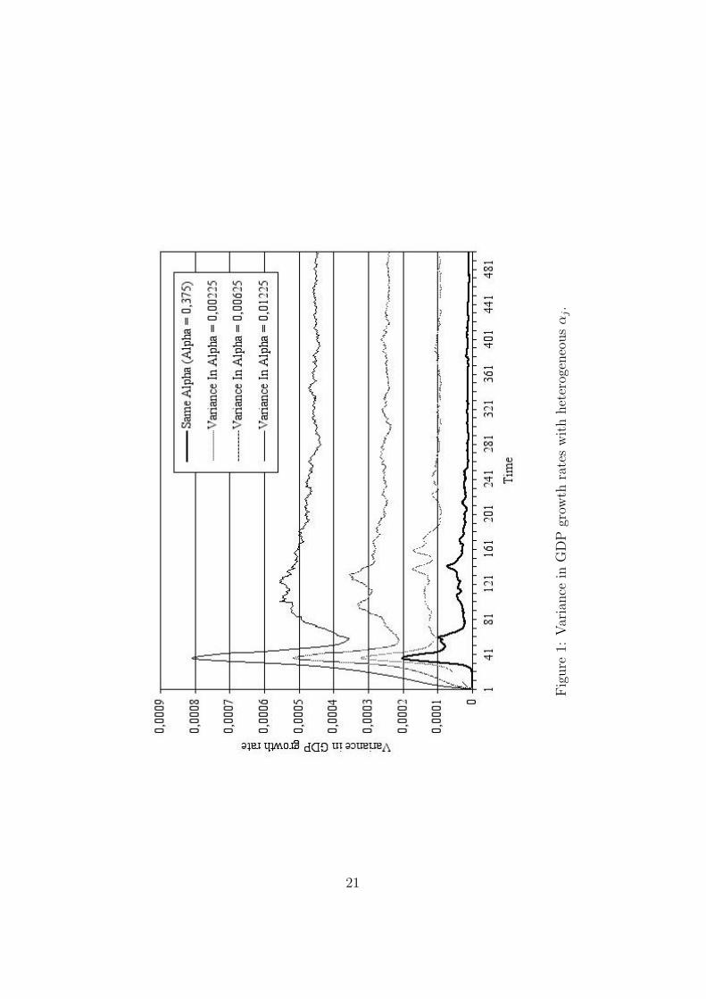
Fig

ure

1:Var

iance

inG

DP

grow

thra

tes

wit

hhet

erog

eneo

usα

j.

21

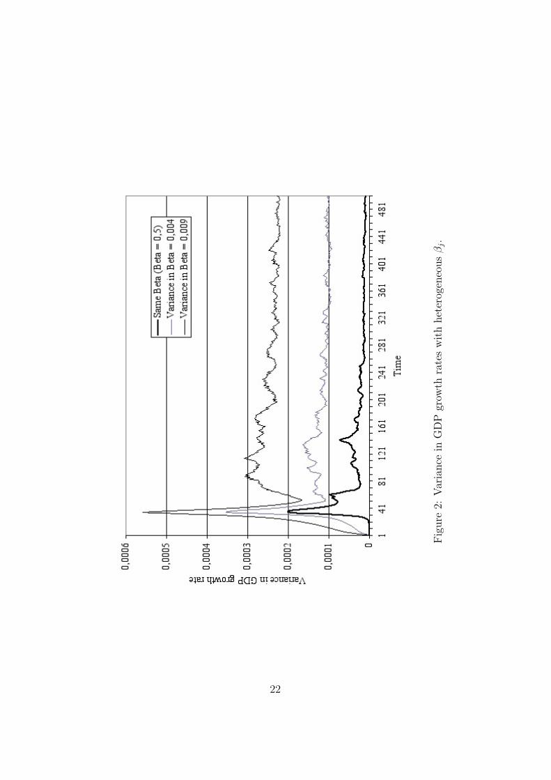
Fig

ure

2:Var

iance

inG

DP

grow

thra

tes

wit

hhet

erog

eneo

usβ

j.

22

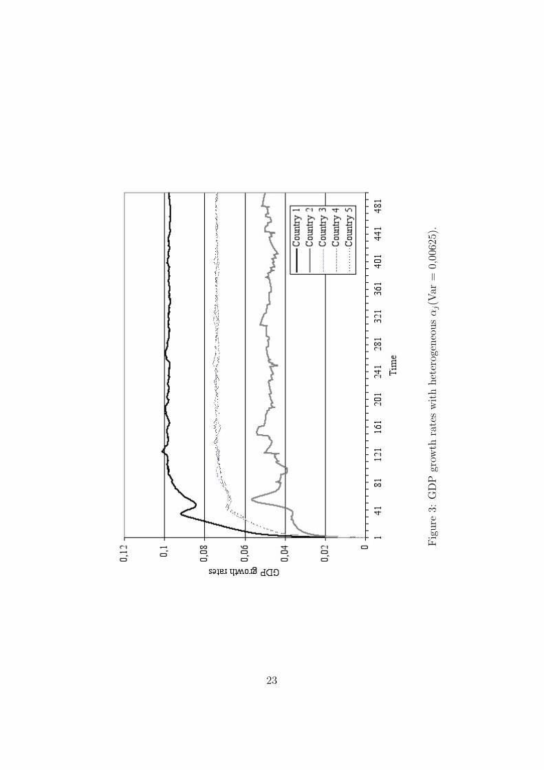
Fig

ure

3:G

DP

grow

thra

tes

with

het

erog

eneo

usα

j(V

ar=

0,00

625)

.

23

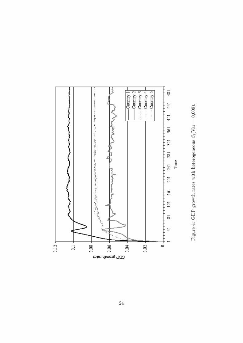
Fig

ure

4:G

DP

grow

thra

tes

with

het

erog

eneo

usβ

j(V

ar=

0,00

9).

24

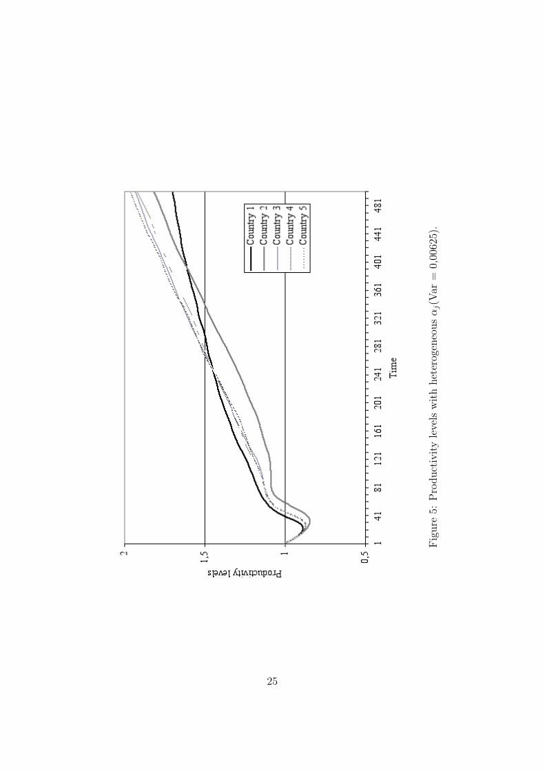
Fig

ure

5:P

roduct

ivity

leve

lsw

ith

het

erog

eneo

usα

j(V

ar=

0,00

625)

.

25

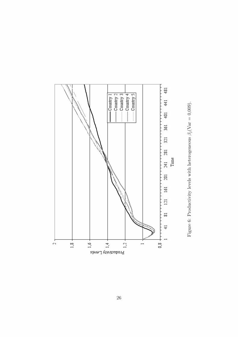
Fig

ure

6:P

roduct

ivity

leve

lsw

ith

het

erog

eneo

usβ

j(V

ar=

0,00

9).

26

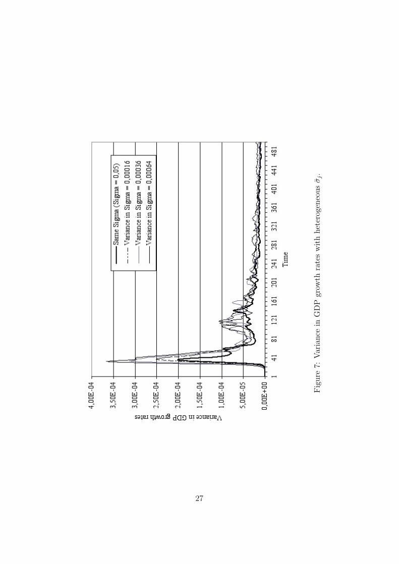
Fig

ure

7:Var

iance

inG

DP

grow

thra

tes

wit

hhet

erog

eneo

usσ

j.

27

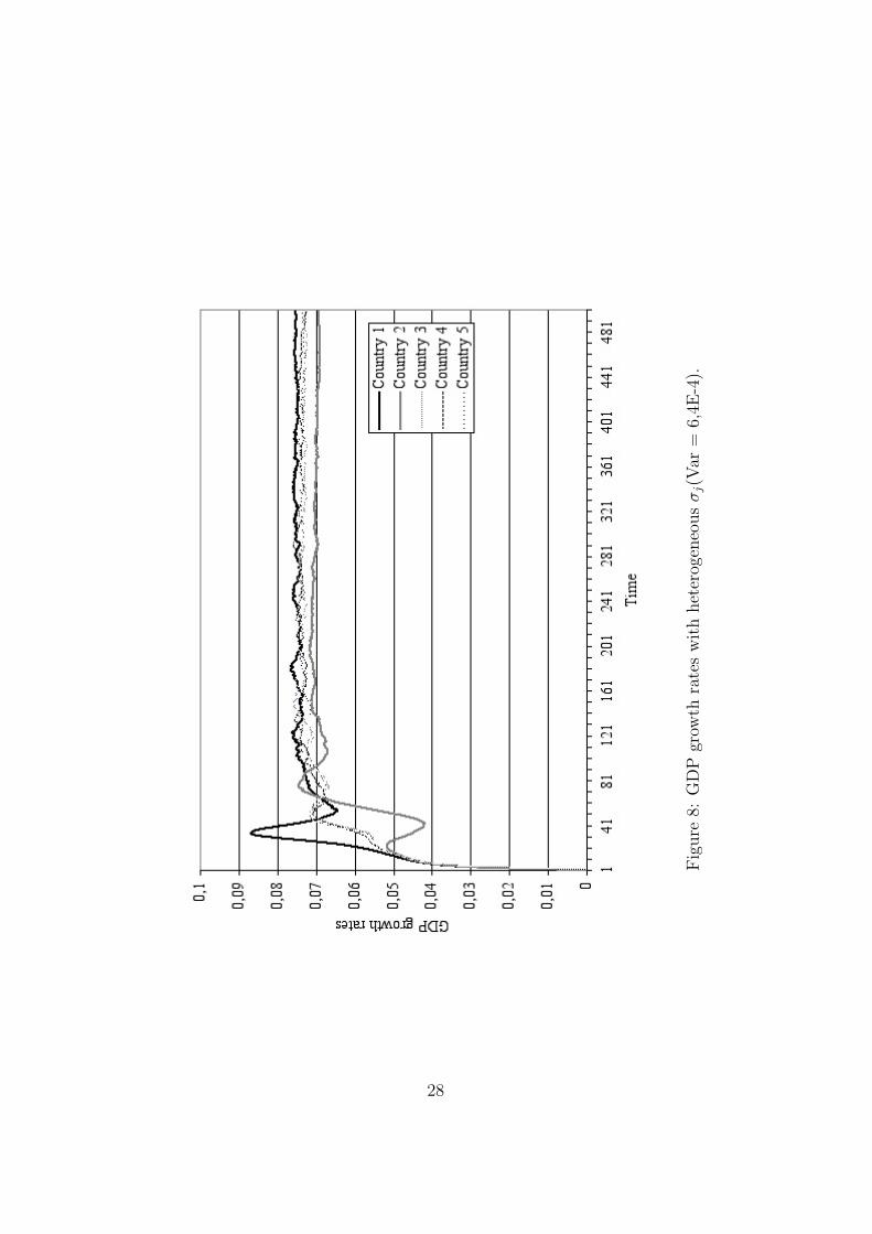
Fig

ure

8:G

DP

grow

thra

tes

with

het

erog

eneo

usσ

j(V

ar=

6,4E

-4).

28

Fig

ure

9:P

roduct

ivity

leve

lsw

ith

het

erog

eneo

usσ

j(V

ar=

6,4E

-4).

29

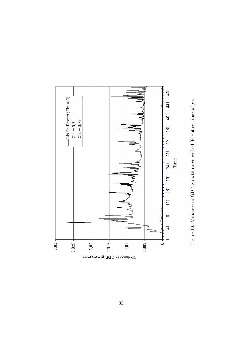
Fig

ure

10:

Var

iance

inG

DP

grow

thra

tes

with

diff

eren

tse

ttin

gsofχ

j.

30

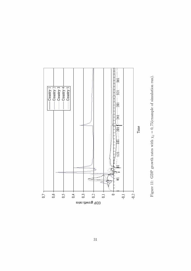
Fig

ure

11:

GD

Pgr

owth

rate

sw

ithχ

j=

0,75

(exam

ple

ofsi

mula

tion

run).

31

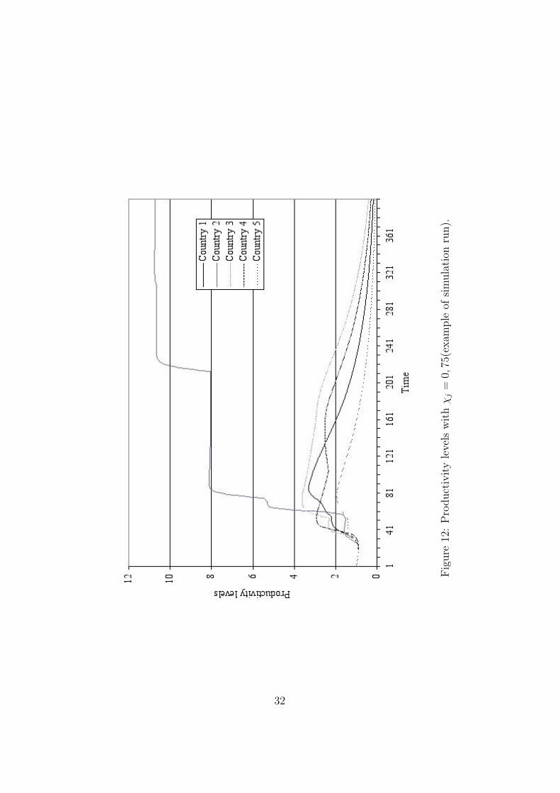
Fig

ure

12:

Pro

duct

ivity

leve

lsw

ithχ

j=

0,75

(exam

ple

ofsi

mula

tion

run).

32

Fig

ure

13:

Var

iance

inG

DP

grow

thra

tes

with

het

erog

eneo

usχ

j.

33