Embed Size (px)
Citation preview
Household Balance Sheet Channels of Monetary Policy:A Back of the Envelope Calculation for the Euro Area∗
Jiri Slacalek†, Oreste Tristani‡ and Giovanni L. Violante§
April 4, 2020
Abstract
This paper formulates a back of the envelope approach to study the effects of monetary policyon household consumption expenditures. We analyze several transmission mechanisms oper-ating through direct, partial equilibrium channels—intertemporal substitution and net interestrate exposure—and indirect, general equilibrium channels—net nominal exposure, as well aswealth, collateral and labor income channels. The strength of these forces varies across house-holds depending on their marginal propensities to consume, their balance sheet composition,the sensitivity of their own earnings to fluctuations in aggregate labor income, and the respon-siveness of aggregate earnings, asset prices and inflation to monetary policy shocks. We quantifyall these channels in the euro area by combining micro data from the HFCS and the EU-LFS withstructural VARs estimated on aggregate time series. We find that the indirect labor income chan-nel and the housing wealth effect are strong drivers of the aggregate consumption response tomonetary policy and explain the cross-country heterogeneity in these responses.
Keywords: Consumption, Euro Area, Hand-to-Mouth, Household Balance Sheets, HouseholdHeterogeneity, Housing, Inflation, Labor Income, Marginal Propensity to Consume, MonetaryPolicy, Wealth Distribution.
JEL codes: D14, D31, E21, E52, E58∗We thank Felipe Alves, Hugo Lhuillier, Adrian Monninger, Alessandro Pizzigolotto and Francisco Rodrigues
for excellent research assistance. We also thank Fernando Alvarez, Rudi Bachmann, Florin Bilbiie, Chris Carroll,Gabriel Chodorow-Reich, Bill Dupor, Nicola Fuchs-Schündeln, Luigi Guiso, Jonathan Heathcote, Geoff Kenny, LucLaeven, Michele Lenza, Davide Malacrino, Benjamin Moll, Dirk Niepelt, Ricardo Reis, Michael Reiter, and ChristianWolf for their comments. We are especially grateful to Ralph Luetticke for his insightful discussion. All opinionsexpressed are personal and do not necessarily represent the views of the European Central Bank or the EuropeanSystem of Central Banks. This paper uses data from the Eurosystem Household Finance and Consumption Survey.†European Central Bank: [email protected], http://www.slacalek.com/‡European Central Bank and CEPR: [email protected]§Princeton University, CEBI, CEPR, IFS, IZA, and NBER: [email protected]

1 Introduction
In the last few years a new literature has flourished in macroeconomics. It embeds New Keyne-sian elements (namely nominal rigidities) into the workhorse incomplete market framework. Acentral contribution of this Heterogeneous Agent New Keynesian (HANK) literature is to revisitthe transmission mechanism of monetary policy (???). In Representative Agent New Keynesianmodels (RANK), monetary policy affects consumption expenditures because households sub-stitute intertemporally between consumption and saving in the wake of unexpected changes inthe interest rate. In HANK, this channel is small and coexists with a plethora of others. First,intertemporal substitution is not the only direct, i.e. partial equilibrium, effect. Changes in theinterest rate affect household financial income differently depending on whether they are bor-rowers or savers (i.e. their net interest rate exposure). Indirect effects operate through the generalequilibrium responses of inputs and asset prices, notably labor income and house prices. Aftera monetary easing, the direct increase in households’ expenditure and firms’ investment stimu-lates output, employment and wages. The additional increases in expenditure induced by higheremployment and wages are the essence of the indirect effect. The strength of these indirect chan-nels crucially depends on the size of the marginal propensity to consume (MPC), which is anorder of magnitude higher in HANK models relative to RANK ones.1
The recent literature on HANK models has followed two parallel paths in order to quantifythese various effects. Some authors have built rich DSGE models by adding a lot of realism on thehousehold side to otherwise standard New Keynesian environment (????????????). Others haveresorted to making simplifying assumptions that lead to analytical solutions (???????). Thesetwo approaches are complements. The first one provides a better framework for the analysisof business cycles and policy counterfactuals. The second one overcomes the computationalcomplexity of the first and offers transparent insights about the economic forces at work.
In this paper, we follow this second approach and apply it to understand the relative strengthof these numerous transmission channels of monetary policy to household spending in the euroarea. In developing the theory, we closely follow ? and formulate an analytical decompositionthat showcases the relevant ingredients needed for this type of back of the envelope calculation.We emphasize that the strength of all transmission channels to aggregate consumption dependson three key dimensions of households’ heterogeneity: their portfolios, their exposures to ag-gregate fluctuations, and their marginal propensities to consume. Distinctly from ?, we arguethat a useful way to summarize such complex distribution is grouping households between thenon-hand-to-mouth, the wealthy hand-to-mouth and the poor hand-to-mouth (HtM) based on
1For a summary of this literature, see e.g., ? and ?.
1

their holdings of liquid and illiquid assets as in ? and ?.2
Our estimation consists of several steps combining aggregate and household-level data forthe four largest euro area countries: Germany, France, Italy, and Spain. From structural VARs, weestimate how monetary policy affects inflation, asset prices, and aggregate employment. Fromthe EU Labor Force Survey (EU-LFS), we estimate the differential systematic sensitivity of thesethree groups to cyclical fluctuations. Micro data on household balance sheets and income fromthe Household Finance and Consumption Survey (HFCS) gives us the distribution of householdportfolios. From the existing literature, we borrow estimates of the MPC out of transitory incomeand capital gains. We then assemble all these ingredients and, guided by our decomposition,provide a back of the envelope calculation that quantifies the impact of a surprise change ininterest rates on household expenditures, separating each channel. Using the estimated responseof aggregate quantities and prices from the VAR to assess the magnitudes of general equilibriumfeedbacks is another key difference between our approach and that of ? and ?.3
At the euro area level we find that about 60 percent of the total increase in nondurable con-sumption is due to the indirect income and housing wealth/collateral channels. Quantitatively,hand-to-mouth households adjust their consumption markedly after the shock. The initial 100basis-point cut of interest rates (80 basis points over a one-year horizon) results in an increase ofconsumption of almost 1 percent for the poor hand-to-mouth and of 1.8 percent for the wealthyhand-to-mouth. Spending of the non-hand-to-mouth households rises by 0.5 percent. Giventheir disproportionate share in consumption (about 80%), the non-hand-to-mouth householdsdominate the aggregate consumption increase of 0.7 percent.
We find that the aggregate consumption response from this simple back of the envelope de-composition matches well the one independently estimated in our structural VAR.
The important role played by the indirect general equilibrium effects implies that a simpleRANK model would underestimate the dynamics of aggregate consumption. The intertemporalsubstitution channel remains the prevalent one only for unconstrained households, and whenwe separate the very rich (top 10 percent) from the rest of the unconstrained, even for them the
2The way to think about these three types of households is the following. Hand to mouth households are at akink in their budget constraint, i.e. they either hold zero liquid wealth (zero is a kink because of the spread betweensaving and borrowing rates) or they are at their unsecured credit limit. The difference between the two types is thatthe wealthy hand-to-mouth ones also hold illiquid wealth (e.g., housing) above a certain threshold. Non hand-to–mouth households are all the rest, i.e. the ‘unconstrained’.
3? and ? share our same goal of estimating the response of consumer spending to monetary policy in the euroarea. They do so through a rich dynamic lifecycle model (i.e. it is more similar to the first approach discussedabove) where households can save in bonds and housing or stocks. Unlike us, their model generates endogenouslythe distribution of MPCs, while we read it off existing evidence. Like us, ? estimate the effects of monetary policyshocks on income and stock returns through a VAR external to the model. A disadvantage of using a large structuralmodel in this context is that its computational complexity prevents them from including nominal debt and the Fisherchannel as well as the housing channel (in case of ?), which we find to be important.
2
indirect effects become dominant because of their extensive holdings of housing and stocks.For the poor hand-to-mouth, all their increase in spending is due to the combination of three
elements: (i) aggregate employment increases after the monetary easing, (ii) their labor incomeis especially sensitive to the cycle, and (iii) their MPC our of transitory income changes is large.
The wealthy hand-to-mouth gain from this same labor income channel. In addition, becausethey tend to be homeowners with large mortgages, they benefit for three reasons. After an inter-est rate cut, house prices rise. Also inflation rises, reducing the real value of debt. This last force,however, is quantitatively modest as a result of the well documented limited response of infla-tion to monetary policy in the euro area. Finally, when they hold flexible rate mortgage contractsthey also take advantage from the reduction in interest payments.
The differences in homeownership rates, mortgage market institutions (prevalence of adjust-able-rate mortgages) and labor market institutions imply that the strength of the transmissionchannels varies considerably across our four euro area economies. We mostly contrast Germanyand Spain, which represent polar cases in terms of these structural factors. For example, house-holds in Spain are almost twice as likely to own their home and also hold much more adjustable-rate debt. The two countries also differ in the share of hand-to-mouth households. Over 17percent of Spanish households are wealthy hand-to-mouth compared to 12 percent in Germany.In addition, we estimate a much stronger sensitivity of aggregate house prices and labor earningsto monetary policy in Spain than in Germany.
Because of all these differences, the income and the housing wealth/collateral effects in Spainsubstantially exceed their counterparts in Germany. Even the direct net interest rate exposureeffect of a cut in the policy rate is large and positive in Spain, whereas it is small and negativein Germany since German households are net savers. When we add up to obtain the total effect,aggregate nondurable consumption responds very strongly in Spain (nearly 2 percent) and muchless so in Germany (0.4 percent).
The rest of the paper is organized as follows. Section ?? outlines our analytical decomposition.Section ?? explains how we empirically implement this decomposition. Section ?? describes ourfindings. Section ?? concludes.
2 Decomposition of effects of a monetary policy shock
We develop an analytical decomposition of the effects of a monetary policy shock on householdconsumption expenditures. The derivation follows closely ?, as well as ? and ?. We proceedstep by step and examine: (i) direct effects of changes in interest rates due to intertemporalsubstitution and (ii) net interest rate exposures, (iii) indirect labor income effects, (iv) Fisher
3
effects due to the reevaluation of nominal long-term assets, and (v) effects associated with capitalgains on real, less liquid, assets such as stocks and housing.
Rather than writing down a complex household problem with all these features at the sametime, we separate these channels and examine each one in isolation. The gains in terms of clar-ity outweigh the tediousness of some repetition, we believe. We begin with the problem ofnon hand-to-mouth unconstrained households and next we analyze the problem of the hand-to-mouth ones. This decomposition will guide our empirical exercise.
We study the effect of a purely transitory change in the (real) policy rate R = 1 + r, i.e. a oneperiod change that has no impact on future values of the interest rate. We assume this shock isunexpected and perceived as ‘once and for all’, i.e. we examine what the literature often callsan MIT shock. This shock has also transitory effects on income, asset prices and inflation (butpermanently changes the price level).4
To simplify the exposition, we abstract from idiosyncratic and aggregate risk. Specifically, weabstract from the fact that a monetary policy shocks can lead to fluctuations in the precautionarysaving motive (and hence in current and future marginal propensity to consume) and shiftsin the share of hand-to-mouth households.5 We only model the effects of monetary policy onconsumption of nondurables and services, and abstract from the adjustment of durables.
Throughout the derivations, we adopt a recursive formulation and denote future variablesby the ‘prime’ sign.
2.1 Non-hand-to-mouth households
Non hand-to-mouth households are those for which borrowing constraints do not bind. Thus,they are on their Euler equation for consumption and saving. We’ll use this property repeatedlyin the derivations below. In particular, we take the extreme view that the constraint never bindsfor them so they are, essentially, permanent-income consumers.
2.1.1 Household problem and marginal propensity to consume
We begin with a statement of the household problem and a derivation of a formula for themarginal propensity to consume (MPC). The household is infinitely lived, with intra-period util-ity u (c), with u′ > 0 and u′′ < 0, where c denote consumption expenditures. Later we specialize
4We adopt this assumption of transitory effects for simplicity, but also because the typical half life of a monetaryshock is 6 months and the reference period in all our empirical analysis is a year. Persistent shocks are analyzed by?, ? and ?.
5The precautionary saving motive at steady-state, however, could be thought of being absorbed into the levelof the marginal propensity to consume which, as we discuss later, we take directly from the data. ? documentmoderate cyclical fluctuations in the share of hand-to-mouth households in the US.
4

the utility function to the CRRA class and let γ ≥ 0 be the coefficient of relative risk aversion.Let b denote holdings of a one-period real asset, and y denote household income. The future isdiscounted at rate 1/β− 1. The recursive formulation of the household problem is:
V (b, y; R) = maxc,b′
u (c) + βV(b′, y′; R) (1)
s.t.
b′ = R (b + y− c)
where R is the initial level of the policy rate.The first-order condition (FOC) with respect to c is
uc = βRV′b , (2)
where we used the notation V′b to denote ∂V(b′, y′; R)/∂b′. Totally differentiating it with respectto c and b′ yields:
uccdc = βRV′bbdb′. (3)
Define the individual marginal propensity to consume for a non HtM household with states(b, y) as the change in consumption induced by a change in wealth:
µ (b, y) :=dcdb
(4)
and note that, by differentiating the budget constraint,
1R
db′ + dc = db (5)
i.e. a marginal dollar of wealth can be either spent or saved. Thus,
µ :=dcdb
= 1− 1R
db′
db, (6)
or, the MPC (where we dropped the arguments to lighten notation) equals one minus the marginalpropensity to save (MPS) adjusted by the interest rate between the two periods. Dividing (??)by db, using it into the above equation and rearranging yields:
µ =R2βV′bb
ucc + R2βV′bb. (7)
5

2.1.2 Direct effects
We begin by considering the effect of a transitory change in R on c, keeping y constant, i.e. whatthe literature calls the direct effect of monetary policy. Combining the FOC (??) and the budgetconstraint yields
uc = βRV′b(
R (b + y− c) , y′; R)
. (8)
Differentiating with respect to R and c yields
uccdc = βV′bdR + βRV′bb (b + y− c) dR− R2βV′bbdc (9)
and note that the value function V′ depends on R only through b′ since next period the interestrate returns to R. Using the FOC (??) in the first term of the right hand side (RHS) and dividingthrough by ucc (c) yields:
dc
[1 +
R2βV′bbucc
]=
uc
ucc
dRR
+R2βV′bb
ucc(b + y− c)
dRR
.
Substituting (??) into the left-hand side and using the approximation dR/R ' dr yields:
dc =uc
ucc(1− µ) dr + µ (b + y− c) dr.
From the definition of the elasticity of substitution for CRRA utility 1/γ := − ucuccc we obtain:
dcDIR = − 1γ(1− µ) cdr + µ (b + y− c) dr. (10)
The first term captures the intertemporal substitution effect (IES). An increase in r induces house-holds to save more, by postponing consumption from today into the future. The substitutioneffect increases in the value of the elasticity of intertemporal substitution 1/γ and the value ofthe marginal propensity to save (1− µ). The second term captures net exposure to the interestrate. An increase in r induces a positive income effect if the household is a net saver (b + y > c)and a negative income effect if it is a borrower. The size of the income effect is proportional tothe MPC µ.
Long-term liquid assets. So far we have assumed that b is a short term (one-period) liquid asset.Generalizing this derivation to long-term liquid assets and liabilities is immediate. Suppose thata fraction δB of assets B and a fraction δ` of liabilities ` matures every period. The most relevant
6
example, in our context, is adjustable rates mortgages (ARMs).6 Then, it is easy to see that theformula in (??) can be generalized to:
dcDIR = − 1γ(1− µ) c dr + µ
[(b + y− c) + δBB− δ``
]dr, (11)
The last three terms in (??), combined in the squared bracket, form what ? calls the net interestrate exposure effect (NIE) of monetary policy, thus:
dcDIR = dcIES + dcNIE.
2.1.3 The indirect general equilibrium effects on income
Instead of fixing y, we now allow labor income y to be affected by r. This channel captures theidea that changes in the interest rate can have so-called ‘aggregate demand effects’, for examplebecause of the presence of nominal rigidities. An initial impulse to expenditures raises labor de-mand and earnings, pushing up expenditures further through an equilibrium multiplier effect.7
Since we only consider transitory changes in r, future income y′ is unaffected.8 Returning toequation (??) and differentiating with respect to c and y we arrive at:[
ucc + R2βV′bb
]dc = R2βV′bbdy. (12)
From the definition of the MPC in (??), we obtain:
dcINC = µdy, (13)
where the last term is the indirect labor income effect (INC). Note that the change in labor incometranslates into consumption proportionately to the MPC µ.
To put more structure on this term, let εy,Y be the elasticity of individual income to aggregateincome. Individuals differ in their age, education, location, industry, occupation, skill level, etc.,and all these characteristics determine a different degree of exposure to aggregate fluctuations.9
6The reduction of interest payments on adjustable rate long term debt is often called in the literature cash-floweffect. See, .eg., ?, ? and ?.
7Even in absence of nominal rigidities, a lower interest rate may expand investment, therefore increasing thecapital stock, the marginal product of labor and the wage.
8Sticky prices slow down dynamics. Our implicit assumption is that, within the time horizon we consider —oneyear— prices, and thus income, have fully adjusted.
9These individual elasticities εy,Y have to satisfy the aggregate consistency condition stating that when theyare summed across all individuals with weights equal to y/Y (the individual income share of the total), such sumequals to one.
7

Then, another useful way to write (??) is
dcINC = µεy,Y
( yY
)dY. (14)
The change in aggregate income produced by the monetary policy shock passes through to con-sumption proportionately to the marginal propensity to consume µ, the sensitivity of individualto aggregate income εy,Y and the individual share of total income y/Y. As discussed in ? and?, unequal incidence of aggregate fluctuations across the population can be a source of dampen-ing or amplification of macro shocks, depending on the covariance between exposure and MPCacross consumers.
2.1.4 Fisher effects through nominal long-term debt
We now extend the household problem to incorporate nominal long-term debt (namely, mort-gages).10 The problem becomes:
V (b, y, m; R, p) = maxc,b′
u (c) + βV(b′, y′, m′; R, p′)
s.t.
b′ = R(
b + y− c− δmmp
)m′ = (1− δm)m
where m is a geometrically decaying stock of nominal debt whose fraction δm matures everyperiod, and p is the aggregate price level. Since we have already analyzed interest exposureeffects earlier, here we assume without loss of generality that the interest rate on these nominalliabilities is zero and focus on the impact of the policy shock on the price level.11 We do not allowthe household to adjust m (i.e. we assume refinancing away), but given the focus on a transitorychange in the policy rate and the well known frictions in refinancing, this simplification is ratherinnocuous.12
The household’s FOC becomes:
uc = βRV′b
(R(
b + y− c− δmmp
), y′, m′; R, p
), (15)
10We note that if long-term debt is nominal, like in the case of most long-term mortgage contracts with adjustablerates, then ` and δ` in Section ?? would equal, respectively, the real value of the contract m/p and its maturityparameter δm in this section.
11The timing we adopted, for convenience, is that the mortgage payment is made at the beginning of the period,at the same time as consumption expenditures.
12?, ? and ?, among others, study the effects of monetary policy through refinancing.
8
where, we have used the fact that, since the price level changes permanently within the period,p′ = p. This rise in the price level will lead to a re-evaluation effect on debt. Differentiating thislast equation with respect to c and p:
uccdc = −βR2V′bbdc + βR2V′bb
(δmm
p
)dpp
+ βRV′bp(b′, y′, m′; R, p
)dp. (16)
Combining the Envelope condition uc = Vb with (??) evaluated at steady state, forwarding oneperiod and differentiating with respect to p:
V′bp = βR2V′′bb
δm (1− δm)mp2 + βRV
′′bp.
Note that V′′bb = V′bb (and similarly for the subsequent periods) because the environment is sta-
tionary after the period of the shock. Under the assumption βR = 1 we can substitute outrecursively the cross derivative of the value function to arrive at
V′bp = RV′bbδmm
p2
∞
∑j=1
(1− δm)j
which combined with (??) yields
uccdc = −βR2V′bbdc + βR2V′bb
(δmm
p
)dpp
+ βRRV′bb
((1− δm)m
p
)dpp
.
For small deviations of the interest rate from steady-state, R/R ' 1, and with the normalizationp = 1 we obtain
dcNOM = µmdp. (17)
This is what the literature calls the Fisher effect (NOM). An interest rate cut that generates inflation(a permanent rise in the price level dp) reduces the real value of debt. The extent to whichcurrent consumption responds to this re-evaluation effect depends on the size of the outstandingnominal liabilities and on the MPC.
2.1.5 Effects through capital gains on real (less liquid) assets
We now allow the household to hold a real asset k such as stocks or housing. Let q be the relativeprice of this asset and normalize its dividend to zero. We assume that only a fraction λ < 1 ofhouseholds react to this price change and, when they do, they must pay a fixed transaction costτ > 0 to adjust their stock of k. Let ∆ > 0 be withdrawals from the illiquid asset for the purpose
9

of reallocating funds into liquid wealth b or consuming it.13 The household problem becomes:
V (b, y, k; R, q) = maxc,b′,k′
u (c) + βV(b′, y′, k′; R, q) (18)
s.t.
b′ = R (b + y− c + ∆)
qk′ = qk− ∆− τI{∆>0}
∆ ≤ θqk
where the last inequality is a collateral constraint stating that the maximum amount that canbe withdrawn is a fraction θ of the value of the asset. Note that, because the change in R istransitory, also q returns to its steady state value after the first period.
Consider a household who adjusts its portfolio (i.e. at the optimum ∆ > 0) and whose col-lateral constraint is not binding. We can split its problem between the consumption/savingdecision in the first stage and the allocation of saving between the two assets in the second stage.Let total financial wealth next period be x′ = b′+ qk′. The first-stage of the problem above, whenall wealth is temporarily liquid, can be therefore restated (with a slight abuse of notation for V)as:
V (b, y, k; R, q) = maxc,x′
u (c) + βV(x′; R, q)
s.t.
x′ = R (b + y− c + qk) .
Differentiating the Euler equation
uc = βRV′x(
R (b + y− c + qk) , y′; R, q)
with respect to c and q, keeping in mind that the effect of a change in the policy rate r on q istransitory, we obtain
uccdc = −βR2V′xxdc + βR2V′xxkdq.
Rearranging, and taking into account that only a fraction λ adjusts following the capital gain,yields the average change for the holders of the real asset:
dcCAP = λµk · dq,
13We focus on the case of a withdrawal (∆ > 0), but the derivation holds for deposits (∆ < 0) as well.
10
where, without loss of generality we have normalized q = 1.The key observation is that the MPC out of a capital gain in illiquid wealth λµ is smaller than
the MPC out of a transitory liquid wealth/labor income change for non hand-to-mouth house-holds (simply µ), because not everyone responds to the price change. This feature of the modelis consistent with the empirical evidence on MPCs out of different types of windfall incomes.
We conclude by noting that, in the context of housing, this calculation is likely to providean upper bound for the effect of a rise in prices for two reasons. First, as discussed by ?, themore transitory the price change, the higher the impact on consumption since more householdswould adjust (i.e. λ is larger). Second, we are abstracting from the fact that some householdsexpect to be homeowners in the future and, as a result of the higher house price, they need tocut expenditures to afford the same housing consumption in the future. This bias, however, issmaller the more transitory the price change is.
2.1.6 Summary
Combining all the pieces together, for a non hand-to-mouth household (denoted with subscriptn) the consumption response at impact to a transitory monetary policy shock is:
dcTOTn = dcIES
n + dcNIEn + dcINC
n + dcNOMn + dcCAP
n ,
which can be unfolded as:
dcTOTndr
= − 1γ(1− µ) cn + µ
[(b + y− cn) + δBB− δ``
](19)
+ µεy,Y
( yY
) dYdr
+ µ ·m · dpdr
+ λµk · dqdr
.
2.2 Hand-to-mouth households
We now develop an analogous derivation for poor and wealthy hand-to-mouth households. Weassume that the constraints that these households face before the shock are still binding after theshock (i.e. the shock is small).
Poor hand-to-mouth. Since they are not on their Euler equation, direct intertemporal substi-tution effects are zero for the poor HtM. Their consumption is fully determined by the budget
11
constraint with b and b′ set at the value of their unsecured credit limit b. If we also allow forsome holdings of nominal debt m with maturing portion δm, we obtain:
c = y− br− δmmp
.
Differentiating the budget constraint with respect to c and R, we obtain
dcNIEp = −b dr. (20)
Comparing (??) to the net interest rate exposure channel for non HtM, (??), the key differenceemerging is the value of the MPC, which is equal to one for the HtM. Differentiating the budgetconstraint with respect to c and p, and normalizing the initial price level p to 1 yields:
dcNOMp = δmmdp, (21)
i.e. for this group the Fisher effect only applies to the currently maturing portion of debt, medi-ated by an MPC equal to one. The indirect income effect, equal to (??), is the only other forceactive for poor HtM households. It is easy to see that differentiating the budget constraint withrespect to c and y we obtain
dcINCp = εy,Y
( yY
)dY (22)
and thus, collecting these three channels the total consumption response of this group can besummarized as:
dcTOTp = dcNIE
p + dcINCp + dcNOM
p ,
or, unfolded,
dcTOTp
dr= −b (23)
+ εy,Y
( yY
) dYdr
+ δmmdpdr
.
Note that, as explained above, some poor hand-to-mouth households are at the zero kink in theirbudget constraint. Since they have no debt, for this subgroup, dcNIE
p = dcNOMp = 0.
Wealthy hand-to-mouth. Direct intertemporal substitution effects are zero also for the wealthyHtM. Since these households might have adjustable rate mortgages in their portfolios besides
12

unsecured debt, their net interest rate exposure component becomes
dcNIEp =
(−b− δ``
)dr. (24)
Fisher and indirect income effects are exactly as for the poor HtM. Because they own someilliquid assets, effects through capital gains are operational for this type of households. In par-ticular, for these households collateral constraints tend to bind, or they would borrow more toconsume more. A constrained household can take advantage of a price change only to the extentthat a rise in the value of collateral relaxes its credit limit and allows him to tap into its illiq-uid wealth. As before let λ be the fraction of households adjusting. Assume that the collateralconstraint
∆ ≤ θqk (25)
is binding. The version of the budget constraint in (??) for a wealthy HtM household is therefore:
c = y + θqk.
Differentiating the above equation with respect to c and q, and accounting for the fact that onlya share λ of households taps into their illiquid wealth, yields (after the normalization q = 1):
dCAP = λθk · dq,
thus λθ is, effectively, the marginal propensity to consume out of the capital gain for this group.In conclusion, the total consumption response for a wealthy HtM household is:
dcTOTw = dcNIE
w + dcINCw + dcNOM
w + dcCAPw
which can be unfolded as:
dcTOTwdr
= −b− δ`` (26)
+ εy,Y
( yY
) dYdr
+ δmmdpdr
+ λθk · dqdr
.
This concludes our theoretical decomposition. We now turn to its empirical implementation.
13
3 Empirical implementation
In practice, we want to measure the impact of a monetary policy shock on non-durable expendi-tures in the first year after the shock.
We follow the strategy adopted for the decomposition and assume that the bulk of the het-erogeneity in the population which is relevant for the monetary policy transmission can be cap-tured by three groups of households: (i) non-hand-to-mouth, (ii) poor hand-to-mouth, and (iii)wealthy hand-to-mouth.
The idea that we leveraged in the decomposition is that HtM households face frictions whichmake their consumption decision insensitive to changes in the interest rate, but highly sensitiveto transitory changes in income. On the contrary, the non HtM are permanent income consumersand thus are insensitive to transitory income shocks but, being on their Euler equation, they areresponsive to changes in the real rate. In addition, these three hand-to-mouth groups differ inthe structure of their balance sheet and, potentially, in their degree of exposure to aggregateincome fluctuations. As clear from our discussion of Section ??, these features are central to thedecomposition.
For each HtM type, we need a number of ingredients. To calculate the intertemporal substitu-tion channel, we need values for the IES 1/γ and the MPCs µ, which we obtain from the existingempirical literature. To compute portfolio exposure to fluctuations in the interest rate, we need ameasure of liquid wealth (b) and saving, which we construct by combining data from the HFCSwith National Accounts data. We measure the indirect labor income effect in two steps. First, weestimate the impact of a monetary policy shock on aggregate earnings through a structural VAR.Second, we estimate the sensitivity εy,Y of labor income of each group to aggregate fluctuationsfrom the EU Labour Force Survey (LFS) data, as done by in ?, ? and ? for the US. To computethe transmission through long-term nominal debt, we use HFCS data on household portfoliosjointly with VAR evidence on the impact of a monetary policy shock on inflation. To calculate theeffects occurring through capital gains, we again estimate the effects of monetary policy shockson asset prices (stocks and housing) through the same VAR, and obtain values of the MPC outof stocks and housing from the literature.
We obtain the total impact of a monetary policy shock on consumption by aggregating theconsumption response of the three groups weighted by their expenditures shares. Upon aggre-gating, we do not impose any equilibrium condition. In particular, we do not impose C = Y,as done by ? and by (?) in their analysis of monetary transmission in the representative agentand in the two-agent New Keynesian model. While this condition establishes some internal con-sistency, it does so only for a closed economy without capital. Instead, we opt for subsuming
14
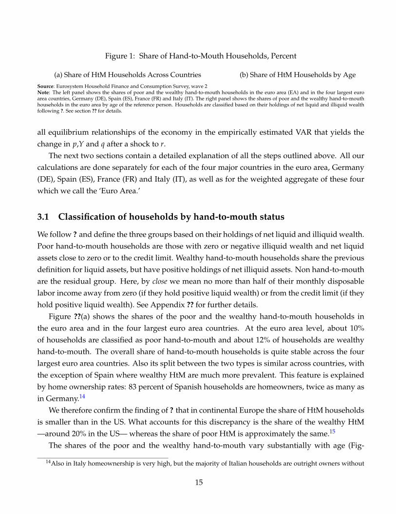
Figure 1: Share of Hand-to-Mouth Households, Percent
(a) Share of HtM Households Across Countries (b) Share of HtM Households by Age
Source: Eurosystem Household Finance and Consumption Survey, wave 2Note: The left panel shows the shares of poor and the wealthy hand-to-mouth households in the euro area (EA) and in the four largest euroarea countries, Germany (DE), Spain (ES), France (FR) and Italy (IT). The right panel shows the shares of poor and the wealthy hand-to-mouthhouseholds in the euro area by age of the reference person. Households are classified based on their holdings of net liquid and illiquid wealthfollowing ?. See section ?? for details.
all equilibrium relationships of the economy in the empirically estimated VAR that yields thechange in p,Y and q after a shock to r.
The next two sections contain a detailed explanation of all the steps outlined above. All ourcalculations are done separately for each of the four major countries in the euro area, Germany(DE), Spain (ES), France (FR) and Italy (IT), as well as for the weighted aggregate of these fourwhich we call the ‘Euro Area.’
3.1 Classification of households by hand-to-mouth status
We follow ? and define the three groups based on their holdings of net liquid and illiquid wealth.Poor hand-to-mouth households are those with zero or negative illiquid wealth and net liquidassets close to zero or to the credit limit. Wealthy hand-to-mouth households share the previousdefinition for liquid assets, but have positive holdings of net illiquid assets. Non hand-to-mouthare the residual group. Here, by close we mean no more than half of their monthly disposablelabor income away from zero (if they hold positive liquid wealth) or from the credit limit (if theyhold positive liquid wealth). See Appendix ?? for further details.
Figure ??(a) shows the shares of the poor and the wealthy hand-to-mouth households inthe euro area and in the four largest euro area countries. At the euro area level, about 10%of households are classified as poor hand-to-mouth and about 12% of households are wealthyhand-to-mouth. The overall share of hand-to-mouth households is quite stable across the fourlargest euro area countries. Also its split between the two types is similar across countries, withthe exception of Spain where wealthy HtM are much more prevalent. This feature is explainedby home ownership rates: 83 percent of Spanish households are homeowners, twice as many asin Germany.14
We therefore confirm the finding of ? that in continental Europe the share of HtM householdsis smaller than in the US. What accounts for this discrepancy is the share of the wealthy HtM—around 20% in the US— whereas the share of poor HtM is approximately the same.15
The shares of the poor and the wealthy hand-to-mouth vary substantially with age (Fig-
14Also in Italy homeownership is very high, but the majority of Italian households are outright owners without
15
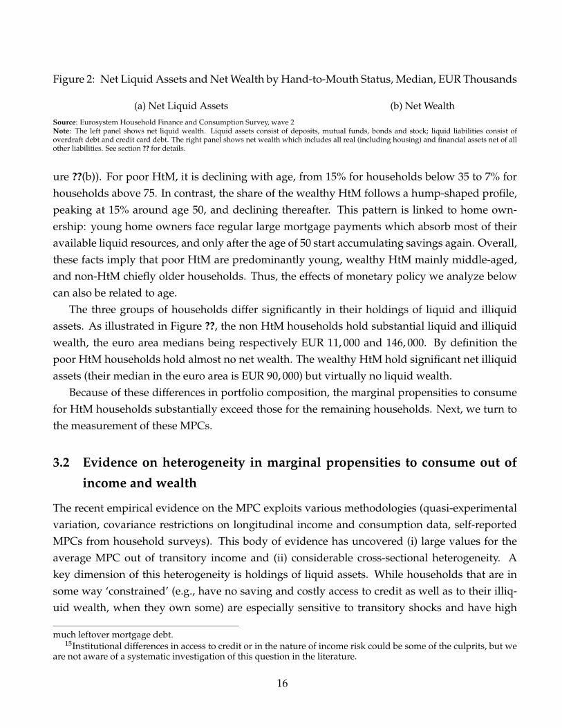
Figure 2: Net Liquid Assets and Net Wealth by Hand-to-Mouth Status, Median, EUR Thousands
(a) Net Liquid Assets (b) Net Wealth
Source: Eurosystem Household Finance and Consumption Survey, wave 2Note: The left panel shows net liquid wealth. Liquid assets consist of deposits, mutual funds, bonds and stock; liquid liabilities consist ofoverdraft debt and credit card debt. The right panel shows net wealth which includes all real (including housing) and financial assets net of allother liabilities. See section ?? for details.
ure ??(b)). For poor HtM, it is declining with age, from 15% for households below 35 to 7% forhouseholds above 75. In contrast, the share of the wealthy HtM follows a hump-shaped profile,peaking at 15% around age 50, and declining thereafter. This pattern is linked to home own-ership: young home owners face regular large mortgage payments which absorb most of theiravailable liquid resources, and only after the age of 50 start accumulating savings again. Overall,these facts imply that poor HtM are predominantly young, wealthy HtM mainly middle-aged,and non-HtM chiefly older households. Thus, the effects of monetary policy we analyze belowcan also be related to age.
The three groups of households differ significantly in their holdings of liquid and illiquidassets. As illustrated in Figure ??, the non HtM households hold substantial liquid and illiquidwealth, the euro area medians being respectively EUR 11, 000 and 146, 000. By definition thepoor HtM households hold almost no net wealth. The wealthy HtM hold significant net illiquidassets (their median in the euro area is EUR 90, 000) but virtually no liquid wealth.
Because of these differences in portfolio composition, the marginal propensities to consumefor HtM households substantially exceed those for the remaining households. Next, we turn tothe measurement of these MPCs.
3.2 Evidence on heterogeneity in marginal propensities to consume out of
income and wealth
The recent empirical evidence on the MPC exploits various methodologies (quasi-experimentalvariation, covariance restrictions on longitudinal income and consumption data, self-reportedMPCs from household surveys). This body of evidence has uncovered (i) large values for theaverage MPC out of transitory income and (ii) considerable cross-sectional heterogeneity. Akey dimension of this heterogeneity is holdings of liquid assets. While households that are insome way ‘constrained’ (e.g., have no saving and costly access to credit as well as to their illiq-uid wealth, when they own some) are especially sensitive to transitory shocks and have high
much leftover mortgage debt.15Institutional differences in access to credit or in the nature of income risk could be some of the culprits, but we
are not aware of a systematic investigation of this question in the literature.
16

Table 1: Calibration of Marginal Propensities to Consume out of Income and Wealth
Marginal Propensity to Consume
CollateralHousehold Type Transitory Income Housing Wealth Stock Market Wealth
Poor Hand-to-Mouth 0.50 – –Wealthy Hand-to-Mouth 0.50 0.07 0.07Non-Hand-to-Mouth 0.05 0.01 0.01
Notes: The table shows the calibrated values of the marginal propensities to consume out of transitory income,collateral / housing wealth and stock market wealth.
marginal propensities to consume out of income, households with adequate liquid assets arewell-insured and do not materially respond. See, e.g., the reviews of the empirical literature by?, ? , Table 1, and ? , Table 1.16
Based on this extensive evidence, an average annual MPC out of income windfalls of 20% forthe US economy appears to be a conservative choice.17 If we fix the MPC of the non HtM to 5%and assume that the nondurable consumption share of HtM households is 0.25 (as documentedby ?), we obtain a value for the annual MPC for HtM households of 0.65. Once again, we stay onthe conservative side and choose a value of 0.50.18 Given the lack of systematic evidence for theeuro area, we adopt these estimates in our calculation (Table ??).
To compute the formulas from Section ??, we also need MPCs out of housing and stock mar-ket wealth. Estimates of the annual average MPC out of wealth tend to be an order of magnitudesmaller than estimates out of transitory income, typically around 5% for the US. Low-liquidityhouseholds are those responsible for most of the effects for both housing and financial wealth(for recent evidence, see ??).19 Stock market wealth tends to be more liquid than housing wealth(which would imply higher MPCs), but also more volatile (which would imply lower MPCs).Overall, the consumption response to stock market capital gains is estimated to be somewhatsmaller, but differences are seldom significant. The literature also finds that in continental Eu-rope the consumption response to housing capital gains is smaller than in the US and the UK
16See also, e.g., ?, ?, ?, ?, and ?.17This value refers to nondurable purchases. The literature (e.g., ??) also estimates MPCs for total consumption
and finds substantially larger values.18We note that, in the stylized theoretical model above, the MPC for hand-to-mouth households is always equal
to 1, but that is simply because we wanted to draw a stark distinction between different types of households andmade assumptions that lead to that outcome.
19For housing, much of the literature emphasizes the importance of the housing collateral channel that alsofeatures in our decomposition (?).
17
(?), possibly due to more rigid mortgage market institutions that make equity withdrawals morecostly. For example ? estimates an annual MPC out of wealth of 3% in the euro area.
In light of these findings, we set the average MPC out of housing and stock-market wealthfor Europe to 0.025 (around half of the US estimate and in the low range of European estimates).We set the MPC for non hand-to-mouth to 0.01. As a result, the MPC for the HtM (computedresidually as we did for income) must be around 7%.20
We conclude by emphasizing that, even though here we treat the MPC as a parameter, we arewell aware that it is an endogenous object and, as such, it is not invariant to the macroeconomicenvironment. Our approach is based on the presumption that the estimates in Table ?? representthe current distribution of MPCs in these countries and that a small temporary shock to theinterest rate would not change the average MPC for these groups.
3.3 Intertemporal substitution and consumption–income ratios
We set the intertemporal elasticity of substitution 1/γ, a parameter only relevant for non HtMhouseholds, to 0.5 based on the extensive reviews of the literature by ? and ?.
The decomposition in equation (??) for non HtM households needs an estimate of their con-sumption–income ratio.21 Unfortunately, the HFCS has neither (complete) information on con-sumption nor on saving flows. We therefore infer the consumption–income ratio for this groupof households by matching the aggregate consumption–income ratio from National Accountsgiven that (i) we know their income shares from the HFCS and (ii) we also know that c = y for allother constrained households. We arrive at nondurable consumption–income ratios around 70–80% for the non HtM, depending on the country; see the top panel of Table ?? (and Appendix ??for details).
3.4 VAR evidence on aggregate effects of monetary shocks
To identify monetary policy shocks, we adopt an approach which is closely related to the useof high-frequency interest rate surprises as external instruments (?). The approach requires adataset of high-frequency financial-market surprises occurring after the policy announcementsfollowing the meetings of the Governing Council of the ECB. We rely on the Euro Area Mone-tary Policy Event Study Database constructed in ?, which reports changes in the median price ofvarious financial assets observed in a close interval around the monetary policy meetings. More
20Other useful references in the literature on wealth effects are, e.g., ?, ? and ? for the US, and ?, ?, ?, and ? forEuropean countries.
21Then, given their income which is available from the HFCS, we can compute y− c.
18
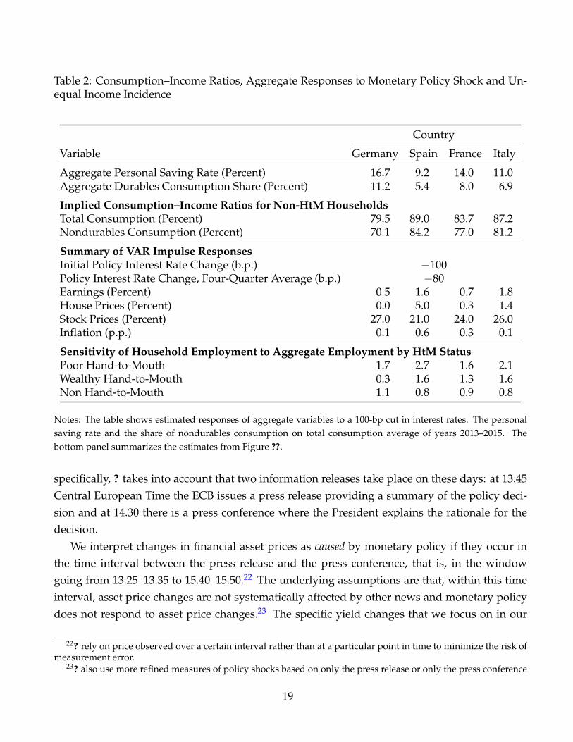
Table 2: Consumption–Income Ratios, Aggregate Responses to Monetary Policy Shock and Un-equal Income Incidence
Country
Variable Germany Spain France Italy
Aggregate Personal Saving Rate (Percent) 16.7 9.2 14.0 11.0Aggregate Durables Consumption Share (Percent) 11.2 5.4 8.0 6.9
Implied Consumption–Income Ratios for Non-HtM HouseholdsTotal Consumption (Percent) 79.5 89.0 83.7 87.2Nondurables Consumption (Percent) 70.1 84.2 77.0 81.2
Summary of VAR Impulse ResponsesInitial Policy Interest Rate Change (b.p.) −100Policy Interest Rate Change, Four-Quarter Average (b.p.) −80Earnings (Percent) 0.5 1.6 0.7 1.8House Prices (Percent) 0.0 5.0 0.3 1.4Stock Prices (Percent) 27.0 21.0 24.0 26.0Inflation (p.p.) 0.1 0.6 0.3 0.1
Sensitivity of Household Employment to Aggregate Employment by HtM StatusPoor Hand-to-Mouth 1.7 2.7 1.6 2.1Wealthy Hand-to-Mouth 0.3 1.6 1.3 1.6Non Hand-to-Mouth 1.1 0.8 0.9 0.8
Notes: The table shows estimated responses of aggregate variables to a 100-bp cut in interest rates. The personalsaving rate and the share of nondurables consumption on total consumption average of years 2013–2015. Thebottom panel summarizes the estimates from Figure ??.
specifically, ? takes into account that two information releases take place on these days: at 13.45Central European Time the ECB issues a press release providing a summary of the policy deci-sion and at 14.30 there is a press conference where the President explains the rationale for thedecision.
We interpret changes in financial asset prices as caused by monetary policy if they occur inthe time interval between the press release and the press conference, that is, in the windowgoing from 13.25–13.35 to 15.40–15.50.22 The underlying assumptions are that, within this timeinterval, asset price changes are not systematically affected by other news and monetary policydoes not respond to asset price changes.23 The specific yield changes that we focus on in our
22? rely on price observed over a certain interval rather than at a particular point in time to minimize the risk ofmeasurement error.
23? also use more refined measures of policy shocks based on only the press release or only the press conference
19
paper refer to Overnight Index Swap (OIS) rates of 1, 3, 6-month and 1 to 10-year maturities. ?report that intraday OIS data are very noisy in the first years of EMU. We therefore ignore 1999data in estimation.
In reality, monetary policy shocks may also include “forward guidance” information aboutfuture changes in policy rates. To abstract from the latter shocks, we proceed following theapproach of ?. We estimate latent factors from changes in yields, select the first two factors, androtate them to ensure that the second one is orthogonal to the first and does not load on the1-month OIS. We can therefore interpret the second factor as a forward guidance factor. In ouranalysis, we focus on the first factor, which represents the current policy surprise.24 We sum allthe intra-day surprises (summarized by the first factor) that occur in given quarter to obtain aquarterly indicator of monetary policy shocks, st.
We introduce the indicator st directly in a quarterly VAR. The key restriction is that st is notaffected contemporaneously by shocks to any of the other VAR variables. This assumption isjustified because st is measured in a narrow time window.25
Beyond the monetary policy surprise indicator, we include in the VAR the following vari-ables: the 3-month nominal interest rate, a commodity price index and, for each of the fourcountries that we consider in our analysis —Germany, France, Italy and Spain— a house priceindex, a consumer price index, real GDP, non-durable consumption, a stock price index, the em-ployment rate, wages, the volume of bank lending and a measure of lending rates. The 3-monthinterest rate, the employment rate and lending rates are measured in annualized percentageterms. All other variables enter the VAR in log-levels.
Given the large number of country-specific variables, we rely on Bayesian estimation meth-ods and use the priors of ?. We generate draws from the posterior using the Gibbs sampler.
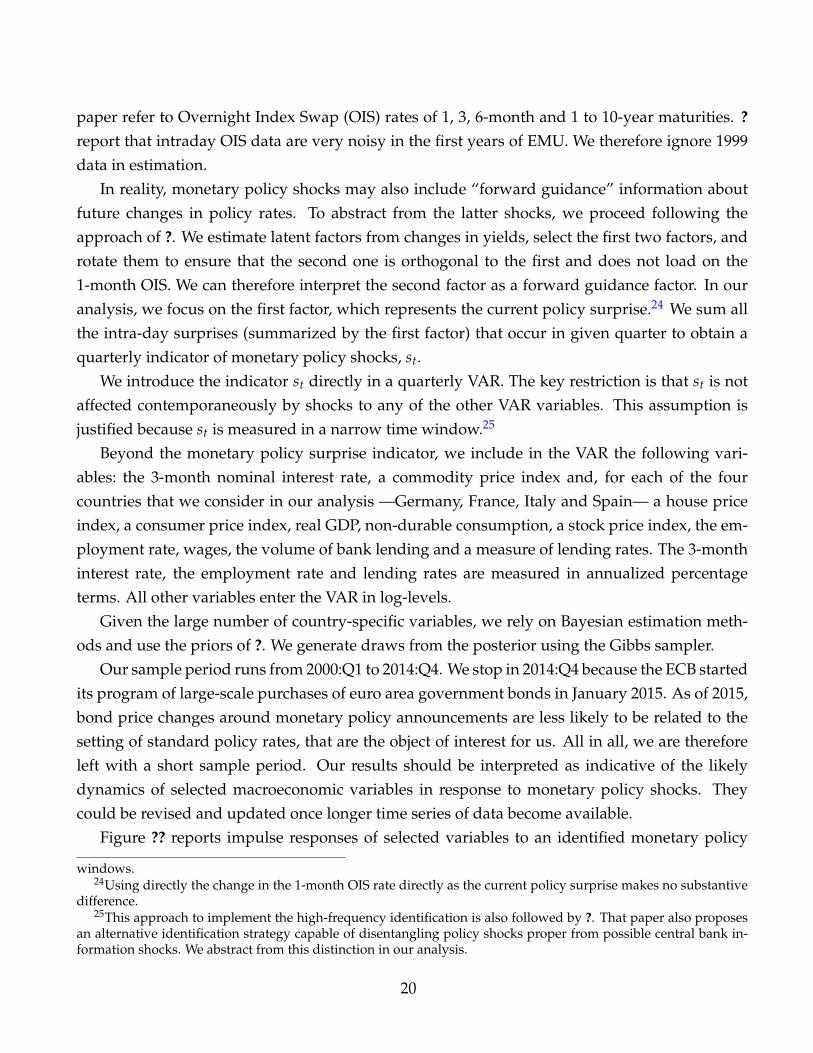
Our sample period runs from 2000:Q1 to 2014:Q4. We stop in 2014:Q4 because the ECB startedits program of large-scale purchases of euro area government bonds in January 2015. As of 2015,bond price changes around monetary policy announcements are less likely to be related to thesetting of standard policy rates, that are the object of interest for us. All in all, we are thereforeleft with a short sample period. Our results should be interpreted as indicative of the likelydynamics of selected macroeconomic variables in response to monetary policy shocks. Theycould be revised and updated once longer time series of data become available.
Figure ?? reports impulse responses of selected variables to an identified monetary policy
windows.24Using directly the change in the 1-month OIS rate directly as the current policy surprise makes no substantive
difference.25This approach to implement the high-frequency identification is also followed by ?. That paper also proposes
an alternative identification strategy capable of disentangling policy shocks proper from possible central bank in-formation shocks. We abstract from this distinction in our analysis.
20
shock leading to a fall of the 3-month nominal interest rate by 100 basis points at impact. Thesolid line shows median responses over 50,000 draws, the darker bands span the 16–84 per-centiles of the draws distribution, the lighter bands cover the percentiles from 5 to 95. By andlarge, impulse responses are only occasionally different from zero from a statistical viewpoint(focusing on the 16–84 percentiles bands). This is to be expected, given our reliance on a high-frequency identification scheme within a large VAR with quarterly data.
There is no commonly agreed benchmark analysis of the effects of ECB monetary policyshocks on individual euro area countries. The broad message from available multi-countrystudies, where policy shocks are often identified through a Cholesky ordering, is that impulseresponses are quite heterogeneous across countries. This is also the gist of our results. For exam-ple, employment rates rise in all countries, but in Spain more so than elsewhere. Similarly, afteran initial drop, house prices go up markedly in Spain, but they are much flatter in Germany. Thisfinding is in line with ?, ? and ?, who investigate the role of the ‘housing transmission channel’and estimate that the monetary policy responses of house prices are stronger in countries wherehouseholds hold more mortgage debt and mortgage contracts are predominantly flexible rate,such as Spain. ?, Figure 8 estimate a semi-elasticity of house prices to interest rates around −4for Spain and ten times smaller for Germany, in line with our findings. We also uncover largeresponses of stock prices to monetary policy shocks. For stock prices, the size of the estimatesreported in the literature varies substantially (see ?, for a survey).
21

Figu
re3:
Impu
lse
Res
pons
esto
100-
bpM
onet
ary
Polic
yEa
sing
Not
es:
Aut
hors
’cal
cula
tion
s.P:
harm
oniz
edC
PI(H
ICP)
,E:e
mpl
oym
ent
rate
,HP:
hous
epr
ices
,SP:
stoc
kpr
ices
,W:w
ages
,CN
D:n
ondu
rabl
esco
nsum
ptio
n.T
heso
lidlin
esh
ows
med
ian
resp
onse
sov
er50
,000
draw
s,th
eda
rker
band
ssp
anth
e16
–84
perc
enti
les
ofth
edr
aws
dist
ribu
tion
,th
elig
hter
band
sco
ver
the
perc
enti
les
from
5to
95.
22

?, Figure 7 also find that the reaction of stock prices to monetary policy is strong, with asemi-elasticity to the interest rate around −20 for most countries. Nevertheless, we consider ourestimate for stock prices to be on the upper bound of the range estimated in the literature.
In the rest of the paper we use the median responses of these variables after 1 year for ourback on the envelope computation. To mitigate the measurement error which could result fromthe choice of a single horizon, we specifically focus on the average impulse response at horizons3 to 5. Table ?? summarizes the estimated impulse responses of employment, consumer prices,house prices and stock prices to a cut to the policy interest rate normalized to an initial size of−100 basis points.
We take into account that the policy rate returns towards the baseline after the initial shock.Thus, to compute the intertemporal substitution and the interest rate exposure components, weuse its average response over the first year, which amounts to an average reduction of 80 basispoints.
3.5 Sensitivity of household eernings to aggregate earnings
From the VAR, we compute the effect of the policy shock on aggregate labor earnings by combin-ing the response of employment and wages in each country. Here we describe how we estimatethe elasticity of household earnings to aggregate earnings for the three types of hand-to-mouthhouseholds.
We use the European Union Labour Force Survey (EU LFS).26 This dataset contains infor-mation about the employment status and demographics of a large sample of households—morethan 100,000 individuals in each country (for ages 15–64).
Even though we are forced to use employment status as a proxy for earnings, because thelatter are not reported in this dataset, we prefer this source to other surveys. The reason is thatsince 2005 the data include the week of the interview. This piece of information allows us tocalculate employment rates at quarterly frequency and combine it with the quarterly time seriesfor aggregate employment.27
We first impute the hand-to-mouth status to households in the LFS from the HFCS using aMincer-style Probit regression of the hand-to-mouth indicator on persistent household charac-teristics: age, education, marital status, gender and sector of occupation. In the LFS, we use thefitted probabilities of belonging to each group to distribute households into the hand-to-mouth
26The EU Labour Force Survey is available at: https://ec.europa.eu/eurostat/web/microdata/
european-union-labour-force-survey; see the appendix in ? for a detailed description of the dataset.27It is also well known that much of the variation of hours worked and total labor income over time is due to the
extensive margin.
23
groups and in doing so we respect, for each country, the shares of the total population in thethree groups estimated from the HFCS.
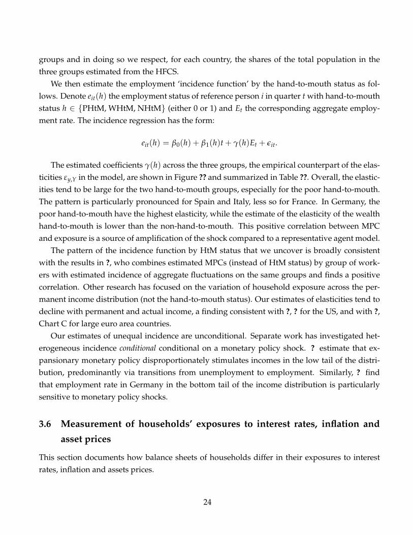
We then estimate the employment ‘incidence function’ by the hand-to-mouth status as fol-lows. Denote eit(h) the employment status of reference person i in quarter t with hand-to-mouthstatus h ∈ {PHtM, WHtM, NHtM} (either 0 or 1) and Et the corresponding aggregate employ-ment rate. The incidence regression has the form:
eit(h) = β0(h) + β1(h)t + γ(h)Et + εit.
The estimated coefficients γ(h) across the three groups, the empirical counterpart of the elas-ticities εy,Y in the model, are shown in Figure ?? and summarized in Table ??. Overall, the elastic-ities tend to be large for the two hand-to-mouth groups, especially for the poor hand-to-mouth.The pattern is particularly pronounced for Spain and Italy, less so for France. In Germany, thepoor hand-to-mouth have the highest elasticity, while the estimate of the elasticity of the wealthhand-to-mouth is lower than the non-hand-to-mouth. This positive correlation between MPCand exposure is a source of amplification of the shock compared to a representative agent model.
The pattern of the incidence function by HtM status that we uncover is broadly consistentwith the results in ?, who combines estimated MPCs (instead of HtM status) by group of work-ers with estimated incidence of aggregate fluctuations on the same groups and finds a positivecorrelation. Other research has focused on the variation of household exposure across the per-manent income distribution (not the hand-to-mouth status). Our estimates of elasticities tend todecline with permanent and actual income, a finding consistent with ?, ? for the US, and with ?,Chart C for large euro area countries.
Our estimates of unequal incidence are unconditional. Separate work has investigated het-erogeneous incidence conditional conditional on a monetary policy shock. ? estimate that ex-pansionary monetary policy disproportionately stimulates incomes in the low tail of the distri-bution, predominantly via transitions from unemployment to employment. Similarly, ? findthat employment rate in Germany in the bottom tail of the income distribution is particularlysensitive to monetary policy shocks.
3.6 Measurement of households’ exposures to interest rates, inflation and
asset prices
This section documents how balance sheets of households differ in their exposures to interestrates, inflation and assets prices.
24
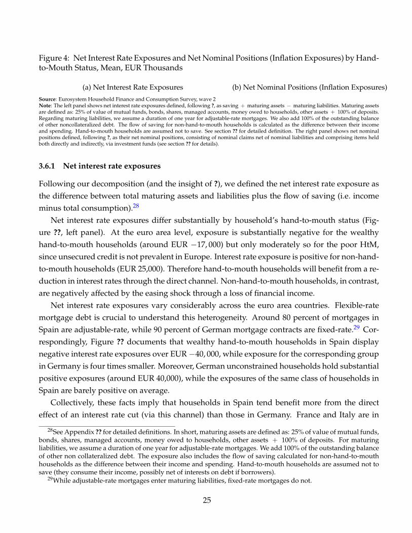
Figure 4: Net Interest Rate Exposures and Net Nominal Positions (Inflation Exposures) by Hand-to-Mouth Status, Mean, EUR Thousands
(a) Net Interest Rate Exposures (b) Net Nominal Positions (Inflation Exposures)
Source: Eurosystem Household Finance and Consumption Survey, wave 2Note: The left panel shows net interest rate exposures defined, following ?, as saving + maturing assets − maturing liabilities. Maturing assetsare defined as: 25% of value of mutual funds, bonds, shares, managed accounts, money owed to households, other assets + 100% of deposits.Regarding maturing liabilities, we assume a duration of one year for adjustable-rate mortgages. We also add 100% of the outstanding balanceof other noncollateralized debt. The flow of saving for non-hand-to-mouth households is calculated as the difference between their incomeand spending. Hand-to-mouth households are assumed not to save. See section ?? for detailed definition. The right panel shows net nominalpositions defined, following ?, as their net nominal positions, consisting of nominal claims net of nominal liabilities and comprising items heldboth directly and indirectly, via investment funds (see section ?? for details).
3.6.1 Net interest rate exposures
Following our decomposition (and the insight of ?), we defined the net interest rate exposure asthe difference between total maturing assets and liabilities plus the flow of saving (i.e. incomeminus total consumption).28
Net interest rate exposures differ substantially by household’s hand-to-mouth status (Fig-ure ??, left panel). At the euro area level, exposure is substantially negative for the wealthyhand-to-mouth households (around EUR −17, 000) but only moderately so for the poor HtM,since unsecured credit is not prevalent in Europe. Interest rate exposure is positive for non-hand-to-mouth households (EUR 25,000). Therefore hand-to-mouth households will benefit from a re-duction in interest rates through the direct channel. Non-hand-to-mouth households, in contrast,are negatively affected by the easing shock through a loss of financial income.
Net interest rate exposures vary considerably across the euro area countries. Flexible-ratemortgage debt is crucial to understand this heterogeneity. Around 80 percent of mortgages inSpain are adjustable-rate, while 90 percent of German mortgage contracts are fixed-rate.29 Cor-respondingly, Figure ?? documents that wealthy hand-to-mouth households in Spain displaynegative interest rate exposures over EUR−40, 000, while exposure for the corresponding groupin Germany is four times smaller. Moreover, German unconstrained households hold substantialpositive exposures (around EUR 40,000), while the exposures of the same class of households inSpain are barely positive on average.
Collectively, these facts imply that households in Spain tend benefit more from the directeffect of an interest rate cut (via this channel) than those in Germany. France and Italy are in
28See Appendix ?? for detailed definitions. In short, maturing assets are defined as: 25% of value of mutual funds,bonds, shares, managed accounts, money owed to households, other assets + 100% of deposits. For maturingliabilities, we assume a duration of one year for adjustable-rate mortgages. We add 100% of the outstanding balanceof other non collateralized debt. The exposure also includes the flow of saving calculated for non-hand-to-mouthhouseholds as the difference between their income and spending. Hand-to-mouth households are assumed not tosave (they consume their income, possibly net of interests on debt if borrowers).
29While adjustable-rate mortgages enter maturing liabilities, fixed-rate mortgages do not.
25

Figure 5: Housing Wealth and Stock Market Wealth by Hand-to-Mouth Status, Mean, EURThousands
(a) Housing Wealth (b) Stock Market Wealth
Source: Eurosystem Household Finance and Consumption Survey, wave 2Note: The left panel shows housing wealth consisting of real estate held as the household main residence and other real estate. The right panelshows stock market wealth owned in directly held stocks (da2105). Both means are calculated as unconditional, i.e. households with no housingor stock market wealth are included as holding EUR 0.
between these two extremes, but closer to Germany in this respect.
3.6.2 Inflation exposures (net nominal positions)
An established literature, at least since ?, has investigated how individual households are af-fected by surprise changes in the price level. Exposures of households to inflation risk are sum-marized by their net nominal positions, consisting of nominal claims net of nominal liabilitiesand comprising items held both directly and indirectly, via investment funds (see section ?? fordetails).
Figure ??, right panel, shows how net nominal positions vary by group. Similar to net interestrate exposures, they are negative for wealthy hand-to-mouth households, who tend to have moremortgage debt than financial assets, and are positive for non-hand-to-mouth households, whosave in financial assets.
Across countries, the major discrepancy in inflation exposures arises between Germany andSpain. In the aggregate, German households hold positive nominal positions and Spanish onesnegative positions. The reason is that savings of German non hand-to-mouth households aresubstantial (EUR 30,000), while those of Spanish non hand-to-mouth households are small.30 Incontrast, inflation exposures of wealthy HtM households in both countries are more comparable.In fact, the median value of mortgage debt (conditional on holding a mortgage) is similar, aroundEUR 70,000, in both countries.
3.6.3 Holdings of housing wealth and stock market wealth
Figure ??, left panel, confirms the well-known fact that housing is the key wealth componentof the wealthy hand-to-mouth households and non-hand-to-mouth households (between EUR140,000–200,000 on average). What is remarkable is that their gross housing wealth is nearly aslarge as that of the non hand-to-mouth ones.
30While the origin of this heterogeneity in portfolios is not strictly relevant for our exercise, we note that a possibledeterminant of differences in current inflation exposures across countries seems to be experienced past inflation, asdocumented by ? and ?.
26
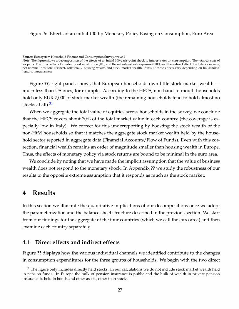
Figure 6: Effects of an initial 100-bp Monetary Policy Easing on Consumption, Euro Area
Source: Eurosystem Household Finance and Consumption Survey, wave 2Note: The figure shows a decomposition of the effects of an initial 100-basis-point shock to interest rates on consumption. The total consists ofsix parts. The direct effect of intertemporal substitution (IES) and the net interest rate exposure (NIE), and the indirect effect due to labor income,net nominal positions (Fisher), collateral / housing wealth and stock market wealth. Sizes of these effects vary depending on households’hand-to-mouth status.
Figure ??, right panel, shows that European households own little stock market wealth —much less than US ones, for example. According to the HFCS, non hand-to-mouth householdshold only EUR 7,000 of stock market wealth (the remaining households tend to hold almost nostocks at all).31
When we aggregate the total value of equities across households in the survey, we concludethat the HFCS covers about 70% of the total market value in each country (the coverage is es-pecially low in Italy). We correct for this underreporting by boosting the stock wealth of thenon-HtM households so that it matches the aggregate stock market wealth held by the house-hold sector reported in aggregate data (Financial Accounts/Flow of Funds). Even with this cor-rection, financial wealth remains an order of magnitude smaller than housing wealth in Europe.Thus, the effects of monetary policy via stock returns are bound to be minimal in the euro area.
We conclude by noting that we have made the implicit assumption that the value of businesswealth does not respond to the monetary shock. In Appendix ?? we study the robustness of ourresults to the opposite extreme assumption that it responds as much as the stock market.
4 Results
In this section we illustrate the quantitative implications of our decompositions once we adoptthe parameterization and the balance sheet structure described in the previous section. We startfrom our findings for the aggregate of the four countries (which we call the euro area) and thenexamine each country separately.
4.1 Direct effects and indirect effects
Figure ?? displays how the various individual channels we identified contribute to the changesin consumption expenditures for the three groups of households. We begin with the two direct
31The figure only includes directly held stocks. In our calculations we do not include stock market wealth heldin pension funds. In Europe the bulk of pension insurance is public and the bulk of wealth in private pensioninsurance is held in bonds and other assets, other than stocks.
27

effects. The figure shows that for non-hand-to-mouth households the intertemporal substitutionchannel (IES) accounts for the bulk of the stimulus and considerably affects aggregate consump-tion (almost 0.4 p.p. out of the total effect of 0.55 p.p.). The interest rate exposure (NIE) raisesconsumption of hand-to-mouth households via lower debt service (on adjustable-rate mortgagesand on other debt), but it slightly reduces consumption of the remaining households who tend tohold positive net interest rate exposures/financial savings.32 In the aggregate, the NIE channeldepresses consumption because the household sector is a net creditor (with respect to the othersectors), but its effect is small.
The figure also illustrates that the indirect effects account for by far the largest part of theconsumption response for the two groups of hand-to-mouth households, 90% (or more) of thetotal effect. The indirect labor income effect is of overwhelming importance to the poor hand-to-mouth households. This channel and the housing wealth/collateral effect are the dominantones for the wealthy hand-mouth households. The Fisher effect via the nominal exposures, turnsout to be quantitatively moderate, except for the wealthy hand-to-mouth, mostly because of thelimited response of inflation to monetary policy easing, but also because of the small size of netnominal positions. The stock market wealth effect is of little importance quantitatively. This isnot surprising given the modest size of stock holdings shown in Figure ??.
Monetary policy shocks impact very differently the three hand-to-mouth groups, both quali-tatively and quantitatively. Qualitatively, the indirect general equilibrium mechanisms are muchmore important for the hand-to-mouth households, while the intertemporal substitution effectis largest for the non-hand-to-mouth households. All in all, about 60 percent of the total increasein aggregate consumption is due to the indirect income and house price channels even at theaggregate level.
Quantitatively, hand-to-mouth households adjust their consumption by considerably morethan the rest of the population after the shock. The initial 100 basis-point cut of interest rates re-sults in an increase of consumption of 1.0 percent for the poor hand-to-mouth and of 1.8 percentof the wealthy hand-to-mouth, while consumption of the non-hand-to-mouth households risesby 0.5 percent. Given their disproportionate share in consumption (about 80%), the non-hand-to-mouth households dominate the total consumption increase of 0.7 percent.
4.2 Cross-country differences
In comparing the results of our decomposition across the four countries, we focus our discussionon Germany and Spain, two ‘polar’ countries in terms of the homeownership rate, the prevalence
32Growing empirical evidence documents this channel is mostly driven by the passthrough of interest rates todisposable income via the debt service/cash flow channel. See ?, ?, ?, ?, ?, ?.
28

Figu
re7:
Effe
cts
ofan
init
ial1
00-b
pM
onet
ary
Polic
yEa
sing
onC
onsu
mpt
ion,
Ger
man
y,Sp
ain,
Fran
ce,I
taly
(a)G
erm
any
(b)S
pain
(c)F
ranc
e(d
)Ita
ly
Sour
ce:E
uros
yste
mH
ouse
hold
Fina
nce
and
Con
sum
ptio
nSu
rvey
,wav
e2
Not
e:T
hefig
ure
show
sa
deco
mpo
siti
onof
the
effe
cts
ofan
init
ial1
00-b
asis
-poi
ntsh
ock
toin
tere
stra
tes
onco
nsum
ptio
n.T
heto
tale
ffec
tco
nsis
tsof
six
part
s;th
edi
rect
effe
ctof
inte
rtem
pora
lsub
stit
utio
nan
dth
ene
tint
eres
trat
eex
posu
rean
dth
ein
dire
ctef
fect
due
toin
com
e,ne
tnom
inal
posi
tion
s(F
ishe
r),c
olla
tera
l/ho
usin
gw
ealt
han
dst
ock
mar
ketw
ealt
h.Si
zes
ofth
ese
effe
cts
vary
depe
ndin
gon
hous
ehol
ds’h
and-
to-m
outh
stat
us.
29
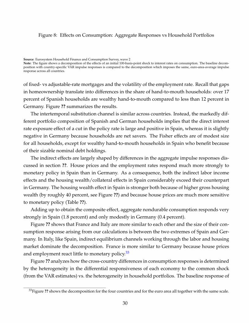
Figure 8: Effects on Consumption: Aggregate Responses vs Household Portfolios
Source: Eurosystem Household Finance and Consumption Survey, wave 2Note: The figure shows a decomposition of the effects of an initial 100-basis-point shock to interest rates on consumption. The baseline decom-position with country-specific VAR impulse responses is compared to the decomposition which imposes the same, euro-area-average impulseresponse across all countries.
of fixed- vs adjustable-rate mortgages and the volatility of the employment rate. Recall that gapsin homeownership translate into differences in the share of hand-to-mouth households: over 17percent of Spanish households are wealthy hand-to-mouth compared to less than 12 percent inGermany. Figure ?? summarizes the results.
The intertemporal substitution channel is similar across countries. Instead, the markedly dif-ferent portfolio composition of Spanish and German households implies that the direct interestrate exposure effect of a cut in the policy rate is large and positive in Spain, whereas it is slightlynegative in Germany because households are net savers. The Fisher effects are of modest sizefor all households, except for wealthy hand-to-mouth households in Spain who benefit becauseof their sizable nominal debt holdings.
The indirect effects are largely shaped by differences in the aggregate impulse responses dis-cussed in section ??. House prices and the employment rates respond much more strongly tomonetary policy in Spain than in Germany. As a consequence, both the indirect labor incomeeffects and the housing wealth/collateral effects in Spain considerably exceed their counterpartin Germany. The housing wealth effect in Spain is stronger both because of higher gross housingwealth (by roughly 40 percent, see Figure ??) and because house prices are much more sensitiveto monetary policy (Table ??).
Adding up to obtain the composite effect, aggregate nondurable consumption responds verystrongly in Spain (1.8 percent) and only modestly in Germany (0.4 percent).
Figure ?? shows that France and Italy are more similar to each other and the size of their con-sumption response arising from our calculations is between the two extremes of Spain and Ger-many. In Italy, like Spain, indirect equilibrium channels working through the labor and housingmarket dominate the decomposition. France is more similar to Germany because house pricesand employment react little to monetary policy.33
Figure ?? analyzes how the cross-country differences in consumption responses is determinedby the heterogeneity in the differential responsiveness of each economy to the common shock(from the VAR estimates) vs. the heterogeneity in household portfolios. The baseline response of
33Figure ?? shows the decomposition for the four countries and for the euro area all together with the same scale.
30
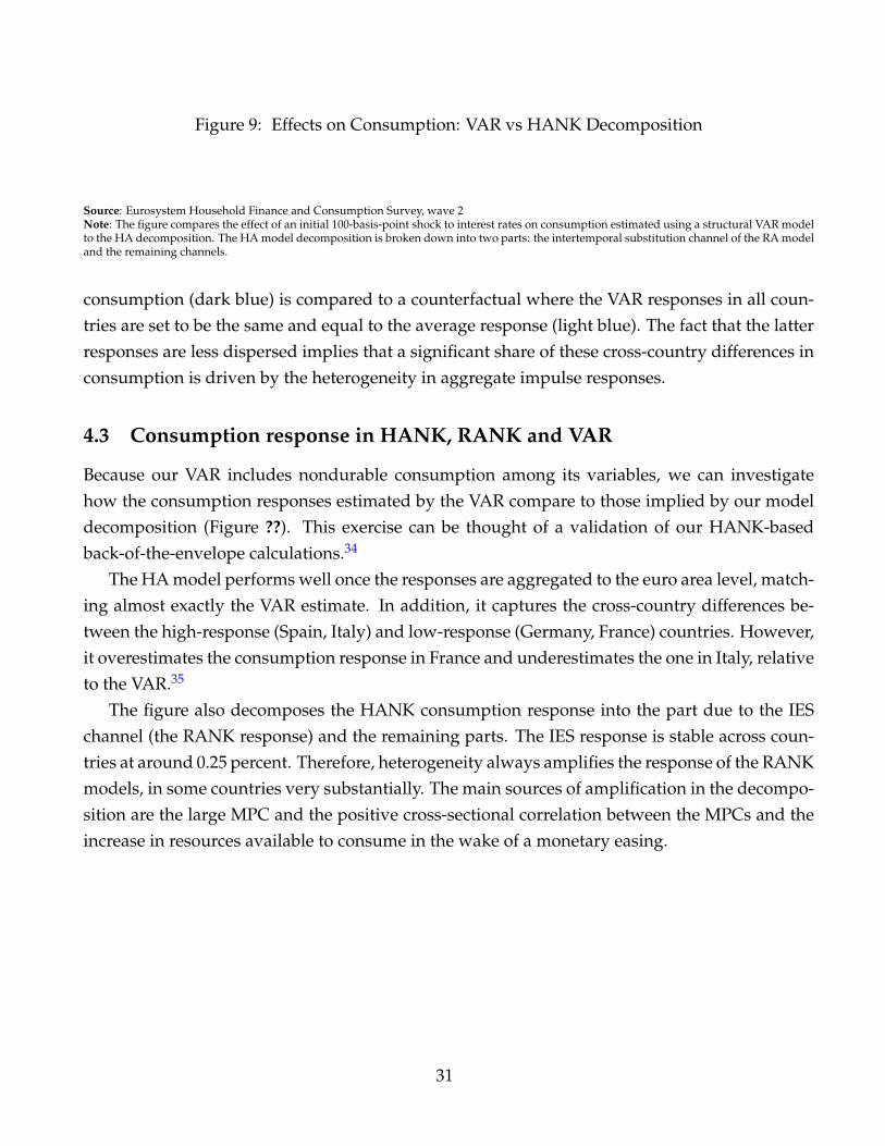
Figure 9: Effects on Consumption: VAR vs HANK Decomposition
Source: Eurosystem Household Finance and Consumption Survey, wave 2Note: The figure compares the effect of an initial 100-basis-point shock to interest rates on consumption estimated using a structural VAR modelto the HA decomposition. The HA model decomposition is broken down into two parts: the intertemporal substitution channel of the RA modeland the remaining channels.
consumption (dark blue) is compared to a counterfactual where the VAR responses in all coun-tries are set to be the same and equal to the average response (light blue). The fact that the latterresponses are less dispersed implies that a significant share of these cross-country differences inconsumption is driven by the heterogeneity in aggregate impulse responses.
4.3 Consumption response in HANK, RANK and VAR
Because our VAR includes nondurable consumption among its variables, we can investigatehow the consumption responses estimated by the VAR compare to those implied by our modeldecomposition (Figure ??). This exercise can be thought of a validation of our HANK-basedback-of-the-envelope calculations.34
The HA model performs well once the responses are aggregated to the euro area level, match-ing almost exactly the VAR estimate. In addition, it captures the cross-country differences be-tween the high-response (Spain, Italy) and low-response (Germany, France) countries. However,it overestimates the consumption response in France and underestimates the one in Italy, relativeto the VAR.35
The figure also decomposes the HANK consumption response into the part due to the IESchannel (the RANK response) and the remaining parts. The IES response is stable across coun-tries at around 0.25 percent. Therefore, heterogeneity always amplifies the response of the RANKmodels, in some countries very substantially. The main sources of amplification in the decompo-sition are the large MPC and the positive cross-sectional correlation between the MPCs and theincrease in resources available to consume in the wake of a monetary easing.
31

Figure 10: Effects on Consumption: The Top 10 Percent
Source: Eurosystem Household Finance and Consumption Survey, wave 2Note: The figure shows a decomposition of the effects of an initial 100-basis-point shock to interest rates on consumption. The total consists ofsix parts. The direct effect of intertemporal substitution (IES) and the net interest rate exposure (NIE), and the indirect effect due to labor income,net nominal positions (Fisher), housing wealth and stock market wealth. Sizes of these effects vary depending on households’ hand-to-mouthstatus. The top 10 percent of households are defined as the 15% of richest households by net wealth among the non-hand-to-mouth (to accountfor the fact that the non-HtM households make up roughly 2/3 of all households).
4.4 The top 10 percent
With our micro data it is easy to further decompose households into more groups. Given thegrowing interest in the widening gap between the richest and the rest of the population we can,for example, analyze how the consumption response to monetary policy shocks for the top 10percent of the wealthiest households differs from that of the rest of the population.36
The top 10 percent of households differ from the rest of the unconstrained households be-cause of their portfolios and their income incidence (see Appendix ?? for details). In terms ofportfolios, the key discrepancy is in the amount of housing they own. While the rest of non-HtMhouseholds own about EUR 120,000 worth of housing in the euro area, the top 10 percent ownover EUR 600,000 in housing. The two groups also differ in the holdings of stocks. The top 10percent of households own about EUR 45,000 in equities, while the rest of the population ownsvirtually no stocks (Figure ??). As for the earnings incidence function, our estimates imply thatthe top 10 percent of households are somewhat more exposed to systematic fluctuations in in-come than the other non-HtM households (except for Spain), a result in line with ? and ? (Figure??).37
The consumption response to monetary policy of the top 10 percent households is strongerthan the response of the other non-HtM households, but still weaker than the response of HtMhouseholds (Figure ??). The key reason for this finding is that the top 10 percent gain substan-tially from increases in asset prices, especially stocks, even though they have a low MPCs. Theirconsumption responses are somewhat dampened by the losses via net interest rate exposures
34Another approach, which we did not follow here, would be to use the consumption responses of the VAR astarget moments and calibrate the MPCs out of capital gains in each country (more likely to vary across countriesthan the MPC out of income because of the institutional differences in restrictions to equity extraction) so that theHANK decomposition matches the VAR responses exactly.
35At least in the case of France, it seems to be the VAR response that is too low (e.g., ? estimate that the consump-tion response in France lies between those of Germany and Italy).
36Because of sample size, we focus on the top 10%. A smaller share would lead to very noisy outcomes.37In all our calculations we assume that this group has the same MPCs as the other non-HtM households, i.e. an
annual MPC out of income 5% and out of capital gains of 1%.
32
and the Fisher channel.
4.5 Accounting for Business Wealth
We conclude with a robustness exercise. Throughout the analysis, we abstracted from privatebusiness wealth. More precisely, we have assumed its value does not react to the shock. Let usnow take the extreme opposite view that business wealth gets reevaluated as much as publiclytraded stocks –recall that stocks react very strongly to an identified monetary easing in the VAR.
Figure ?? in Appendix ?? shows that this assumption has important consequences for theconsumption response of the top 10 percent. This finding was expected in light of the wellknown fact that many among the richest households are entrepreneurs. Under this alternativeassumption, their response more than doubles. What is more surprising is that also expendituresof the wealthy hand-to-mouth group react substantially more. The reason is that, for manyhouseholds in this group, business equity is a large component of their illiquid wealth.
Overall, in this exercise the share of indirect effects of monetary policy exceeds 70%, com-pared to 60% in the baseline.
5 Conclusion
In this paper we formulated a back of the envelope approach to quantify the various transmis-sion mechanisms of monetary policy to household consumption in the four largest countries inthe euro area. Our decomposition illustrates that these channels operate with different strengthacross the distribution of households, depending on households’ marginal propensity to con-sume, portfolio composition, and exposure to aggregate fluctuations —all dimensions whereheterogeneity is sizable.
We argued that a particularly helpful distinction, to summarize this large heterogeneity, isone that groups households in three classes: non hand-to-mouth, wealthy hand-to-mouth andpoor hand-to-mouth based on their holdings of liquid and illiquid wealth.
By combining cross-country micro data on income and household portfolios with estimatesfrom structural VARs on the impact of monetary policy on employment, inflation, and assetprices, we obtained all the ingredients we need to quantify the channels of transmission.
Our main finding is that the general equilibrium effects of an unexpected monetary easingon households’ labor income, through an expansion in aggregate demand and an incrementin house prices, are the principal determinants of the effect of monetary policy on aggregateconsumption across countries. This finding suggests that households with low liquidity account
33
for the lion share of the consumption response to monetary policy shocks. We also uncoveredsignificant differences across countries: Germany displays the weakest response and Spain thestrongest one to a common monetary shock.
Monitoring the composition of household balance sheets and the heterogeneous consequencesof monetary policy across the distribution is therefore important to gain a better understandingof the monetary policy transmission mechanism.
While our analysis focuses on standard interest rate shocks, a similar approach can be taken toanalyze the effects on unconventional monetary policy instruments, such as quantitative easing.For this set of measures, we would expect indirect general equilibrium effects to account for aneven larger share of the total effect because the key channels of transmissions are a boost in assetprices and an expansion in aggregate demand. Who benefits more across the distribution willdepend on the relative strength of these two forces (and whether house prices react more or lessthan stock prices).
Our methodology can also be applied to firms to assess the mechanisms through which mon-etary policy impacts aggregate investment. A quantitative literature which builds on traditionalfirm dynamics models is developing in parallel to that on heterogeneous household (??), butsimple back of the envelope calculations of the type we did in this paper —that can give a pre-liminary idea of the magnitudes without the need for solving complex dynamic equilibriummodels— are so far missing from this literature.
A limitation of the methodology implemented in this paper is that, because of the first-orderapproach taken in the decomposition and the linearity of the VAR, we cannot address nonlin-earities and asymmetries between positive and negative shocks, nor we can examine the roleof time-varying precautionary saving and hand-to-mouth status. The alternative approach fol-lowed in the HANK literature, which quantifies the transmission channels of monetary policythrough richer calibrated or estimated DSGE models, is much more useful in this respect espe-cially when globally solved nonlinearly. As discussed, ? and ? offer a compromise between thesetwo approaches.
We think that the two methodologies should dialogue to best advance the HANK literature.The main lesson we learned here is that incorporating into richer HANK models endogenousmechanisms that lead to realistic fluctuations in individual earnings and asset prices is of first-order importance. Progress in this direction is already being made. For example, ? integrates ajob ladder and ? heterogeneity in risk aversion into HANK models.
34
A Measurement of variables
A.1 Definition of hand-to-mouth households
This section classifies the three groups of households by their hand-to-mouth status. The variable names
refer to wave 2 of the Household Finance and Consumption Survey (HFCS).
Following ?, a household is considered as ‘hand-to-mouth’ if:
• Net liquid wealth ≥ 0 AND net liquid wealth ≤ biweekly (net) income
OR
• Net liquid wealth < 0 AND net liquid wealth ≤ biweekly (net) income − credit limit
A household is:
1. ‘Poor hand-to-mouth’ if it is hand-to-mouth AND net illiquid wealth ≤ 0,
2. ‘Wealthy hand-to-mouth’ if it is hand-to-mouth AND net illiquid wealth > 0,
3. Non-hand-to-mouth if it is not hand-to-mouth.
There are two (small) differences to ?. First, we classify all hand-to-mouth households with some housing
assets (da1110 or da1120) as wealthy hand-to-mouth, including households ‘under water’ whose mort-
gage exceeds the value of the house. Second, we classify all hand-to-mouth households with some self-
employment business wealth (da1140) as wealthy hand-to-mouth.
The variables above are defined as follows:
• Net liquid wealth = liquid assets − liquid liabilities
• Liquid assets = sight and saving accounts (deposits), directly held mutual funds, bonds and stocks
= da2101 + da2102 + da2103 + da2105
• Liquid liabilities = overdraft debt and credit card debt = dl1210 + dl1220
• Net illiquid wealth = illiquid assets − illiquid liabilities
• Illiquid assets = illiquid real assets, value of household main residence and other properties and
value of self-employment businesses = da1110 + da1120 + da1140 + total(pf0710) + da2109
• Illiquid liabilities = amount of non-collateralized loans for household main residence and other
properties, mortgage debt
Credit limit is assumed at one month of income.
35
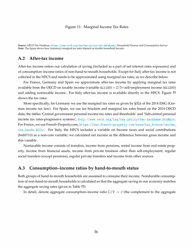
Figure 11: Marginal Income Tax Rates
Source: OECD Tax Database, https://www.oecd.org/tax/tax-policy/tax-database/; Household Finance and Consumption SurveyNote: The figure shows how (statutory) marginal tax rates depend on taxable household income.
A.2 After-tax income
After-tax income enters our calculation of saving (included as a part of net interest rates exposures) and
of consumption–income ratios of non-hand-to-mouth households. Except for Italy after-tax income is not
collected in the HFCS and needs to be approximated using marginal tax rates, as we describe below.
For France, Germany and Spain we approximate after-tax income by applying marginal tax rates
available from the OECD on taxable income (variable di1100) + 2/3×self-employment income (di1200)
and adding nontaxable income. For Italy after-tax income is available directly in the HFCS. Figure ??
shows the tax rates.
More specifically, for Germany we use the marginal tax rates as given by §32a of the 2014 EStG (Ger-
man income tax law). For Spain, we use tax brackets and marginal tax rates based on the 2014 OECD
data; the tables ‘Central government personal income tax rates and thresholds’ and ‘Sub-central personal
income tax rates-progressive systems’, http://www.oecd.org/tax/tax-policy/tax-database.htm#pit.
For France, we use French-Property.com, https://www.french-property.com/news/tax_france/income_
tax_bands_2014/. For Italy, the HFCS includes a variable on Income taxes and social contributions
(hnG0710) as a non-core variable; we calculated net income as the difference between gross income and
this variable.
Nontaxable income consists of transfers, income from pensions, rental income from real estate prop-
erty, income from financial assets, income from private business other than self-employment, regular
social transfers (except pensions), regular private transfers and income from other sources.
A.3 Consumption–income ratios by hand-to-mouth status
Both groups of hand-to-mouth households are assumed to consume their income. Nondurable consump-
tion of non-hand-to-mouth households is calculated so that the aggregate saving in our economy matches
the aggregate saving rates (given in Table ??).
In detail, denote aggregate consumption–income ratio C/Y = c (the complement to the aggregate
36
personal saving rate):
c =CH + CNH
Y=
YH + CNH
Yc×Y = YH + CNH
CNH = c×Y− yH ×YCNH
YNH =c− yH
yNH
where yH is the income share of HtM households (yH = YH/Y).
Assuming the share of nondurable on total consumption is the same for HtM and NHtM households,
we get for nondurable consumption:CNH
ndYNH = cnd ×
c− yH
yNH ,
where cnd is the aggregate share of nondurables consumption to total consumption, cnd = Cnd/C.
A.4 Net interest rate exposure
Net interest rate exposure is calculated following ? (see also ? and ?).
• Interest rate exposure = Income− Total consumption + Maturing assets−Maturing liabilities.
• Regarding the flow of saving (Income−Total consumption), we assume it is zero for hand-to-mouth
households and its value for non-hand-to-mouth households is calculated so that it matches the
aggregate saving rate (see ??).
• Maturing assets = 25% of (mutual funds, bonds, shares, managed accounts, money owed, other
assets) + 100% of deposits.
• Maturing Liabilities = duration of 1 year for ARM + 100% Outstanding balance of non-mortgage
debt38
• Outstanding balance of non-mortgage debt is defined as outstanding balance of credit line/overdraft,
credit card debt and other non-mortgage loans.
A.5 Inflation exposures (net nominal positions)
Net nominal position is calculated following ? and ?:
• Household net nominal position = Net financial position− Indirect nominal position
38The duration of 1 year for ARMs is a conservative estimate for the euro area, estimated following ?. For the US? estimates the duration of three quarters.
37

• Net financial position = Financial assets− Total debt
• Indirect nominal position = Value of mutual funds (da2102) + Non-self-employment private busi-
ness (da2104) + Publicly traded shares (da2105)
38

B Additional results on the top 10 percent households
Figure 12: Housing Wealth and Stock Market Wealth for the Top 10 Percent, Mean, EUR Thou-sands
(a) Housing Wealth (b) Stock Market Wealth
Source: Eurosystem Household Finance and Consumption Survey, wave 2Note: The left panel shows housing wealth consisting of real estate held as the household main residence and other real estate. The right panelshows stock market wealth owned in directly held stocks (da2105). Both means are calculated as unconditional, i.e. households with no housingor stock market wealth are included as holding EUR 0.
39
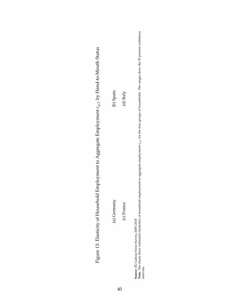
Figu
re13
:Ela
stic
ity
ofH
ouse
hold
Empl
oym
entt
oA
ggre
gate
Empl
oym
entε
y,Y
byH
and-
to-M
outh
Stat
us
(a)G
erm
any
(b)S
pain
(c)F
ranc
e(d
)Ita
ly
Sour
ce:E
ULa
bour
Forc
eSu
rvey
,200
5–20
18N
ote:
The
char
tssh
owes
tim
ated
elas
tici
ties
ofho
useh
old
empl
oym
entt
oag
greg
ate
empl
oym
entε
y,Y
for
the
four
grou
psof
hous
ehol
ds.
The
rang
essh
owth
e95
perc
entc
onfid
ence
inte
rval
s.
40
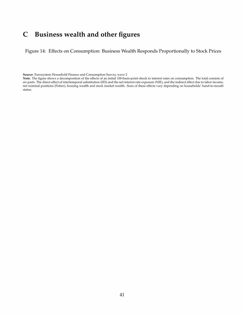
C Business wealth and other figures
Figure 14: Effects on Consumption: Business Wealth Responds Proportionally to Stock Prices
Source: Eurosystem Household Finance and Consumption Survey, wave 2Note: The figure shows a decomposition of the effects of an initial 100-basis-point shock to interest rates on consumption. The total consists ofsix parts. The direct effect of intertemporal substitution (IES) and the net interest rate exposure (NIE), and the indirect effect due to labor income,net nominal positions (Fisher), housing wealth and stock market wealth. Sizes of these effects vary depending on households’ hand-to-mouthstatus.
41

Figu
re15
:Ela
stic
ity
ofIn
divi
dual
toA
ggre
gate
Empl
oym
entε
y,Y
byH
and-
to-M
outh
Stat
us
(a)G
erm
any
(b)S
pain
(c)F
ranc
e(d
)Ita
ly
Sour
ce:E
ULa
bour
Forc
eSu
rvey
,200
5–20
18N
ote:
The
char
tssh
owes
tim
ated
elas
tici
ties
ofho
useh
old
empl
oym
ent
toag
greg
ate
empl
oym
ent
ε y,Y
for
the
thre
eha
nd-t
o-m
outh
grou
psof
hous
ehol
ds.
The
rang
essh
owth
e95
perc
entc
onfid
ence
inte
rval
s.
42

Figu
re16
:Ef
fect
sof
anin
itia
l100
-bp
Mon
etar
yPo
licy
Easi
ngon
Con
sum
ptio
n,G
erm
any,
Spai
n,Fr
ance
,Ita
ly
Sour
ce:E
uros
yste
mH
ouse
hold
Fina
nce
and
Con
sum
ptio
nSu
rvey
,wav
e2
Not
e:T
hefig
ure
show
sa
deco
mpo
siti
onof
the
effe
cts
ofan
init
ial1
00-b
asis
-poi
ntsh
ock
toin
tere
stra
tes
onco
nsum
ptio
n.T
heto
tale
ffec
tco
nsis
tsof
six
part
s;th
edi
rect
effe
ctof
inte
rtem
pora
lsub
stit
utio
nan
dth
ene
tint
eres
trat
eex
posu
rean
dth
ein
dire
ctef
fect
due
toin
com
e,ne
tnom
inal
posi
tion
s(F
ishe
r),h
ousi
ngw
ealt
han
dst
ock
mar
ketw
ealt
h.Si
zes
ofth
ese
effe
cts
vary
depe
ndin
gon
hous
ehol
ds’h
and-
to-m
outh
stat
us.
43