364 Advanced Steel Construction – Vol. 15 No. 4 (2019) 364–376 DOI:10.18057/IJASC.2019.15.4.7

MODELING THE LOCAL BUCKLING FAILURE OF

ANGLE SECTIONS WITH BEAM ELEMENTS

Farshad Pourshargh1, Frederic P. Legeron2,4 and Sébastien Langlois3,*

1 Ph.D. candidate at Université de Sherbrooke, Sherbrooke, Canada

2 Eng., Ph.D. Formerly Professor, Civil Engineering Department, Université de Sherbrooke, Sherbrooke, Canada

3 Eng., Ph.D. Assistant professor, Civil Engineering Department, Université de Sherbrooke, Sherbrooke, Canada

4 Present affiliation: Vice President, Parsons, Dubai, UAE

*(Corresponding Author: Email address: Sebastien.Langlois@USherbrooke.ca)

A B S T R A C T ARTICLE HISTORY

Slender steel sections are widely used in the construction of steel structures such as lattice structures for transmission li ne

and telecommunication towers. Local buckling may be the observed failure mode under compression loads for these slender

sections, and many experimental studies have been conducted to evaluate their resistance. All steel design codes include

equations to account for local buckling. In numerical models, local buckling can be reproduced using 2D shell or 3D

elements. Nonlinear numerical models have been developed in the last decades that can capture the complex behavior of

lattice structures up to failure. These models typically use beam elements that consider correctly the global buckling and

yielding of sections but do not consider the local buckling of angles due to geometrical limitations. This article proposes a

method that modifies the material behavior of sections to involve the local buckling failure in the analysis. Forty -two

experimental tests were conducted on short angles and a general stress-strain formula was defined based on the test results.

The formula relates the local buckling slenderness ratio of the members to a material constitutive law that accounts for the

local buckling. To evaluate the method, the numerical results were compared to those of four x-braced frame configurations

using slender angle sections. The results demonstrate that the proposed method can accurately model the local buckling

failure of fiber beam elements.

Received:

Revised:

Accepted:

11 January 2019

26 February 2019

17 July 2019

K E Y W O R D S

Lattice steel tower;

Angle section;

Local buckling;

Finite element model;

Nonlinear behavior;

Fiber beam element

1. Introduction

Angle steel members are widely used in steel lattice structures for

transmission lines and telecommunications. Lattice towers that are made of

angle members exhibit complex structural behavior, which is mainly due to

connection eccentricity, bolt slippage, local buckling and their impacts on

failure modes. The standard procedure for designing tower members is to

build a simple linear model of the structure for determining the forces in each

member and to evaluate the resistance using design code equations. This type

of analysis may not be correct because the buckling resistance should be

verified as an integrated part of the design and not as an independent stage

[1, 2]. To overcome the limitations of this simple analysis, transmission line

lattice towers are typically tested under various load conditions in full-scale

field tests prior to mass production.

Prasad Rao [3] reported that 32 towers out of 138 full-scale tests at the

Structural Engineering Research Centre [CSIR-SERC] experienced various

types of premature failures, which demonstrates the limitations of the design

method that is used in practice. To study the failure in detail, they modeled

three towers and analyzed them using the NE-Nastran nonlinear finite

element software. The option for geometric and material nonlinearity in the

software was used to obtain the behavior and limit loads. The entire tower

was modeled using beam-column elements. However, to capture more details,

the failed compression bracings were modeled as plate elements. The test

failure pattern coincided with the analysis failure pattern for both beam and

plate modeling. However, nonlinear finite element analysis predicted a failure

load that was 7 to 14 percent higher than the test results.

Another study was performed by the same researchers [4] on five

prematurely failed towers. They encountered overprediction of the strength

by nonlinear analysis and concluded that finite element analysis is still not a

fully reliable method for predicting tower strength and the tests remain

necessary for this objective. However, it is indicated that the nonlinear

analysis is essential for understanding the behavior, load carrying capacity,

design deficiencies, and instability in the structure. This type of nonlinear

model aims at capturing the complex and nonlinear behavior of steel lattice

structures. It is not a practical design method because it does not rely on

design code equations or more advanced methods such as the direct strength

method (DSM) [5, 6, 7] to evaluate the resistance of sections. It provides a

one-step numerical model for representing the pre- and post-buckling

behaviors of the structure. This type of model is useful as an alternative or

complement to full-scale tests for understanding the behavior and evaluating

the resistance of lattice towers. Recent works showed that depending on the

objective of the modeling, the following characteristics of lattice behavior

might need to be considered: joint eccentricity [8, 9], bolt slippage [10], and

residual stresses [11], among others. However, in this type of model, which

normally simulates the elastoplastic buckling of angle members, the potential

local buckling of members is neglected. This article will focus on developing

an efficient method to account for local buckling in nonlinear models of

lattice structures.

Currently, most research on the modeling of angle members uses either

beam elements or 2D shell elements. Angle sections may undergo global or

local buckling instability under a compression load, depending on the

slenderness and the width-to-thickness ratios. Shell elements can represent

the full three-dimensional behavior of angle sections and local buckling with

high accuracy if the mesh is sufficiently refined. However, for large and

complex structures such as lattice towers, the high number of members render

the use of shell elements impractical. For example, Shan et al. [12], proposed

modeling angle members by nonlinear plate elements. They included both

material and geometric nonlinearities in the study; however, the analysis

procedure was computation-intensive and time-consuming. They concluded

that 2D elements can only be used for small structures and as a research tool.

This conclusion has been supported by other researchers [13].

In slender angle sections with a high width-to-thickness ratio, the global

buckling deformation is accompanied by local buckling of leg plates [14] and

this effect should be incorporated into the finite element model of the

structure. Lee and McClure [13] developed an L-section beam finite element

for elastoplastic large deformation analysis. In terms of the computational

time, the beam element is 2.4 times more efficient than shell modeling if the

member length is equal to 4 meters.

The fiber beam element is a highly effective element that is used with

success to model angle sections. This element can properly incorporate the

stress and yielding effects in the member. Kitipornchai et al. [19, 20] reported

an analysis with nonlinear fiber elements of angle sections under axial and

bending loads. Numerical studies were conducted on various structures and

the angle members were modeled as fiber elements. Several examples were

presented to demonstrate the satisfactory performance of the fiber element

model in predicting the ultimate behavior of imperfect angle columns. The

results that were obtained from the study were compared to experimental tests

on two pairs of angle trusses with web members.

Vieira et al. [21] and Carrera et al. [22] proposed a 1D beam element for

modeling the buckling of beams using analytical formulas. The results

accorded with finite element models. Several limitations in capturing the local

buckling behavior were reported. According to the authors, additional tests

and experiments are needed for extending the method.

Farshad Pourshargh et al. 365

Other computational methods for calculating the buckling loads of thin-

walled sections were studied. Huang et al. [23] developed a mathematical

formulation. They considered the angle section as an example and conducted

a numerical analysis of the elastic and inelastic buckling using finite element

models. The results from beam and shell elements were compared with the

theoretical results. It was concluded that the mathematical solution of higher

order differential equations is complicated and for members with complicated

deflections another method should be applied.

Considering other research and experiments in this field, the approach with

fiber elements is well adapted analytically for modeling the transmission

tower structures; however, a full local buckling behavior that covers the pre-

and post-buckling behaviors is not well defined.

The objective of this paper is to propose a method for incorporating the

local buckling behavior in the finite element model of structures using fiber

beam elements by developing a stress-strain behavior curve of steel. Forty-

two slender section angle members were tested and full force-deflection

curves were extracted. Then, a local buckling slenderness ratio was defined

via the direct strength method [5] and equations were developed to relate the

slenderness ratio to two specified points on the stress-strain curve.

Considering these two points, full stress-strain equations were defined by

using curve fitting techniques to model the compressive behavior of a slender

angle with a specified slenderness ratio. Finally, the proposed method was

evaluated by comparing its results to the test results on four full-scale X-

braced frames of angle slender members that were obtained by Morissette

[24].

2. Short angle specimens

2.1. Local buckling slenderness

The experimental program consists of testing 42 short angle members

under pure compression. These tests were conducted to evaluate the global

stress-strain behavior of angles that are failing due to local buckling. To

characterize the sections that are undergoing local buckling, Table 1

introduces the local buckling slenderness ratio, which is denoted as 𝜆𝑝 and is

defined in Equation 1. This ratio is used in the direct strength method [31]

and was found to be useful for relating the properties of the angle to the stress-

strain behavior.

𝜆𝑝 = √𝐹𝑦

𝜎𝑐𝑟 (1)

In this equation, 𝐹𝑦 stands for the yielding stress of steel and 𝜎𝑐𝑟 is the

critical elastic local buckling stress for the member, which can be calculated

using finite element software such as Code_Aster, ANSYS or ABAQUS. In

this study, a finite strip software, namely, CUFSM, which is developed by

Schafer [32], will be used to perform critical elastic buckling load calculations.

CUFSM, which has been developed to accompany the direct strength method,

is a finite strip elastic buckling analysis application. In the first step, the

geometry of the member is modeled either manually or using a built-in cross-

section library. Then, general end boundary conditions and loading are

applied to the member and the section is meshed automatically with finite

strips. Finally, the analysis provides the buckling mode shapes of the member

and the critical elastic buckling load for each mode. This software is freely

available.

In practice, FE analysis is time-consuming for engineers. However, as a

simplification, a mathematical relation can be developed between the local

buckling stress and the width-to-thickness ratio b/t, where b is the width of

the angle leg and t is the thickness of the leg. Based on all the angle members

that are reported in Table 1, a formula is presented that relates 𝜎𝑐𝑟 and ratio

(b/t):

(𝑏

𝑡) =

𝛼

√𝜎𝑐𝑟 (2)

where the value of α is calculated to be 323 according to the curve fitting

analysis that is shown in Fig. 1. In this work, the modulus of elasticity of steel

was assumed to be 200,000 MPa. This simplification can be used when the

boundary conditions of the angle member are fixed translation and free

rotation. However, as shown in Fig. 1, the discrepancy in the local buckling

stress can be important, especially at low b/t values. Therefore, for higher

precision, the full procedure that is presented in the next sections, which

involves a finite element model, is recommended.

Fig.1 Calculated curve that relates 𝜎𝑐𝑟 and (b/t) values

2.2. Experimental program

The objective of the experimental program is to provide test results on

local buckling behavior from specimens of various geometries. Forty-two

short angle specimens, which are listed in Table 1, were tested under pure

compression and the force-deformation behavior was measured. The leg

width-to-thickness ratio, namely, (b/t), of the specimens ranged from 9.5 to

19. According to (CSA-S16) [25] and Eurocode 3 [27], all specimens are

classified as class 4 sections, which are subject to local buckling prior to

yielding under compression. The steel grade of the specimens is ASTM-A36

[28] and their material properties are listed in Table 1.

The lengths of specimens were selected to avoid global buckling

instability. Most configurations were tested on two identical specimens to

evaluate the repeatability of results. The average result of these identical tests

was considered the final result to better represent the types of sections that

are available in the market. Since the specimens are short and they fail under

the local buckling mode, the effects of geometrical imperfections and residual

stresses are not considered. These effects are more important on global

buckling mode, which is outside the scope of this article. Taking the discussed

effects in consideration adds additional parameters to the prediction, which

renders finding a solution highly complicated; hence, these effects are not

investigated further in this article.

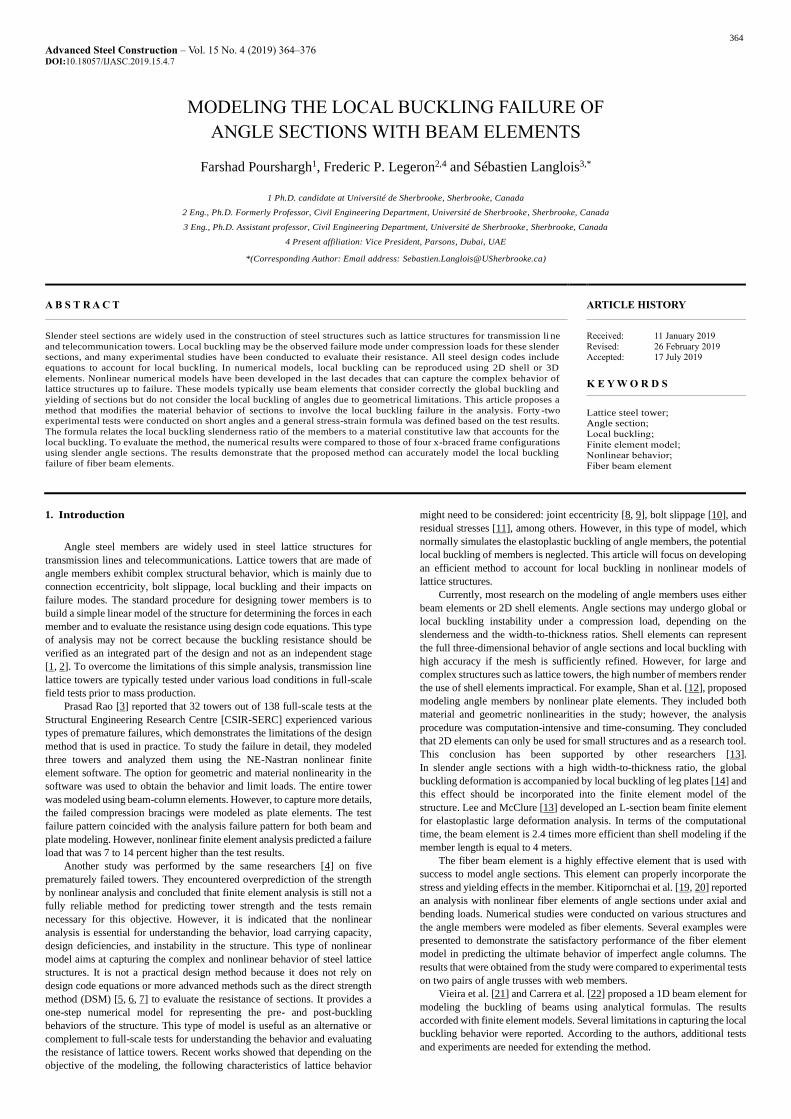
To provide continuous and uniform end conditions throughout the tests,

the extremities of all specimens were accurately milled flat and strictly

perpendicular to the axis of the angle. The specimens were supported by a

thick steel plate without a hinge for the test. The alignment of the centroid of

the angle with the line of action of the force was secured by top and bottom

adjustment plates (Fig. 2) that were bolted to the thick plates. To avoid any

eccentric moment, the center of the force that was applied by the machine

coincided with the center of gravity of the section. The angle-shaped opening

in each set of adjustment plates provided the required end constraints: fixed

translation and free rotation.

Farshad Pourshargh et al. 366

Fig. 2 Adjustment plate in the supports

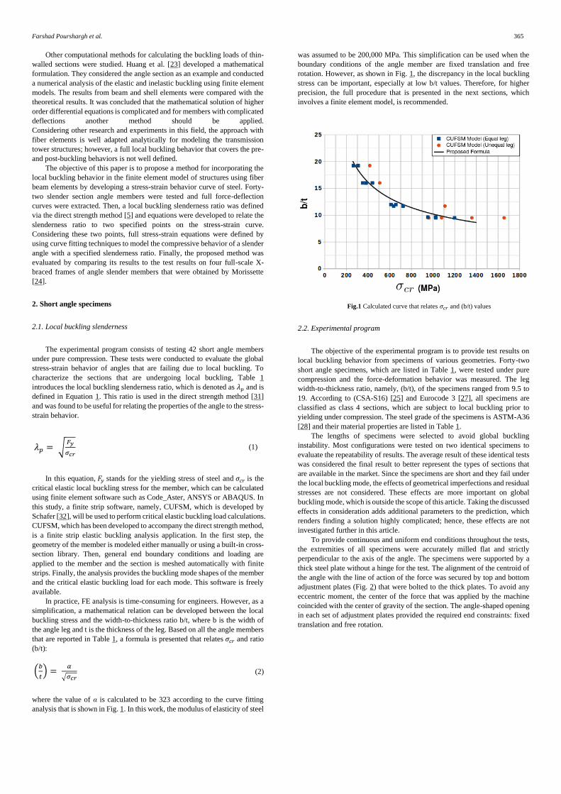
Table 1

Properties of the short angle test specimens

Test Section Length (mm) b/t 𝐹𝑦 (MPa) 𝐹𝑢 (MPa) E (MPa) 𝜎𝑐𝑟 (MPa) 𝜆𝑝

1 L152x152x7.9 600 19.2 339 519 178000 264 1.13

2 L152x152x7.9 600 19.2 339 519 178000 264 1.13

3 L152x152x7.9 400 19.2 339 519 178000 308 1.05

4 L152x152x7.9 400 19.2 339 519 178000 308 1.05

5 L152x152x9.5 600 16 390 543 207000 381 1.01

6 L152x152x9.5 600 16 390 543 207000 381 1.01

7 L152x152x9.5 400 16 390 543 207000 440 0.94

8 L152x152x9.5 400 16 390 543 207000 440 0.94

9 L152x152x16 600 9.5 395 514 188281 1026 0.62

10 L152x152x16 600 9.5 395 514 188281 1026 0.62

11 L152x152x16 400 9.5 395 514 188281 1199 0.57

12 L152x152x16 400 9.5 395 514 188281 1199 0.57

13 L152X102X9.5 433 16 373 495 206297 508 0.86

14 L152X102X9.5 437 16 373 495 206297 508 0.86

15 L152X102X16 438 9.5 375 564 212700 1359 0.53

16 L152X102X16 439 9.5 375 564 212700 1359 0.53

17 L152X102X16 680 9.5 375 564 212700 1080 0.59

18 L152x152x9.5 598 16 392 541 201000 381 1.01

19 L152x152x9.5 597 16 392 541 201000 381 1.01

20 L152x152x9.5 598 16 392 541 201000 381 1.01

21 L152X102X9.5 718 16 371 492 208000 440 0.92

22 L152x152x9.5 850 16 380 526 210000 350 1.04

23 L152X102X16 800 9.5 375 563 212700 960 0.63

24 L152X102X16 300 9.5 375 563 212700 1657 0.48

25 L152X102X16 800 9.5 375 563 212700 960 0.63

26 L152x152x13 850 11.7 388 547 202626 636 0.78

27 L152x152x13 850 11.7 388 547 202626 636 0.78

28 L152x152x13 500 11.7 388 547 202626 723 0.73

29 L152x102x13 800 11.7 407 587 193387 727 0.75

30 L152x102x13 800 11.7 407 587 193387 727 0.75

31 L152x102x13 300 11.7 407 587 193387 1110 0.61

32 L152x102x7.9 800 19.2 405 557 204017 302 1.16

33 L152x102x7.9 800 19.2 405 557 204017 302 1.16

34 L152x102x7.9 300 19.2 405 557 204017 416 0.99

Farshad Pourshargh et al. 367

35 L76x76x6.35 400 12 379 526 203000 612 0.79

36 L76x76x6.35 400 12 379 526 203000 612 0.79

37 L76x76x6.35 300 12 379 526 203000 657 0.76

38 L76x76x6.35 300 12 379 526 203000 657 0.76

39 L76x76x7.9 400 9.6 388 555 203000 952 0.64

40 L76x76x7.9 400 9.6 388 555 203000 952 0.64

41 L76x76x7.9 300 9.6 388 555 203000 1024 0.62

42 L76x76x7.9 300 9.6 388 555 203000 1024 0.62

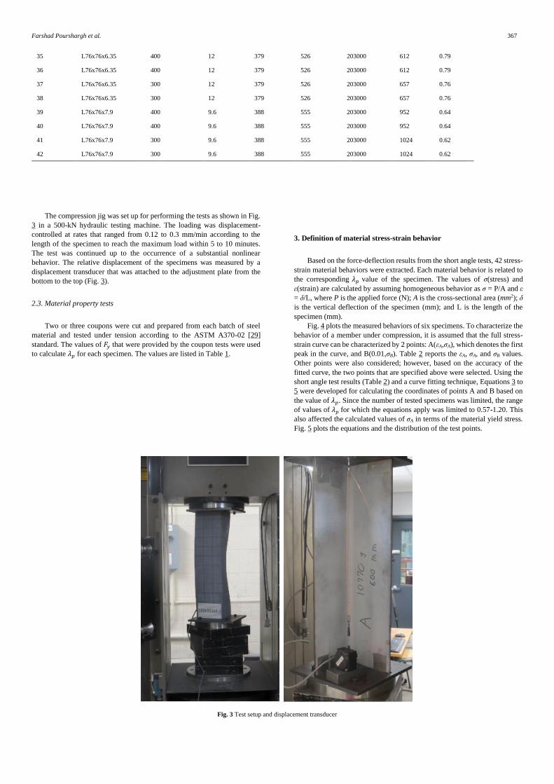
The compression jig was set up for performing the tests as shown in Fig.

3 in a 500-kN hydraulic testing machine. The loading was displacement-

controlled at rates that ranged from 0.12 to 0.3 mm/min according to the

length of the specimen to reach the maximum load within 5 to 10 minutes.

The test was continued up to the occurrence of a substantial nonlinear

behavior. The relative displacement of the specimens was measured by a

displacement transducer that was attached to the adjustment plate from the

bottom to the top (Fig. 3).

2.3. Material property tests

Two or three coupons were cut and prepared from each batch of steel

material and tested under tension according to the ASTM A370-02 [29]

standard. The values of 𝐹𝑦 that were provided by the coupon tests were used

to calculate 𝜆𝑝 for each specimen. The values are listed in Table 1.

3. Definition of material stress-strain behavior

Based on the force-deflection results from the short angle tests, 42 stress-

strain material behaviors were extracted. Each material behavior is related to

the corresponding 𝜆𝑝 value of the specimen. The values of σ(stress) and

ε(strain) are calculated by assuming homogeneous behavior as σ = P/A and ε

= δ/L, where P is the applied force (N); A is the cross-sectional area (mm2); δ

is the vertical deflection of the specimen (mm); and L is the length of the

specimen (mm).

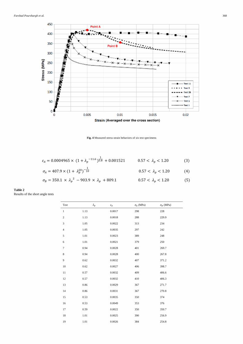
Fig. 4 plots the measured behaviors of six specimens. To characterize the

behavior of a member under compression, it is assumed that the full stress-

strain curve can be characterized by 2 points: A(εA,σA), which denotes the first

peak in the curve, and B(0.01,σB). Table 2 reports the εA, σA, and σB values.

Other points were also considered; however, based on the accuracy of the

fitted curve, the two points that are specified above were selected. Using the

short angle test results (Table 2) and a curve fitting technique, Equations 3 to

5 were developed for calculating the coordinates of points A and B based on

the value of 𝜆𝑝. Since the number of tested specimens was limited, the range

of values of 𝜆𝑝 for which the equations apply was limited to 0.57-1.20. This

also affected the calculated values of σA in terms of the material yield stress.

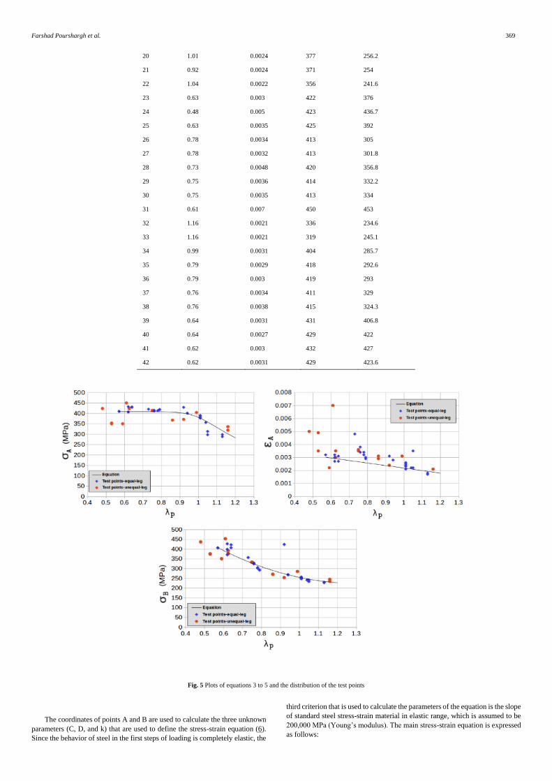
Fig. 5 plots the equations and the distribution of the test points.

Fig. 3 Test setup and displacement transducer

Farshad Pourshargh et al. 368

Fig. 4 Measured stress-strain behaviors of six test specimens

𝜀𝐴 = 0.0004965 × (1 + 𝜆𝑝−11.6 )

15.8 + 0.001521 0.57 < 𝜆𝑝 < 1.20 (3)

𝜎𝐴 = 407.9 × (1 + 𝜆𝑝20)−

110 0.57 < 𝜆𝑝 < 1.20 (4)

𝜎𝐵 = 350.1 × 𝜆𝑝2 − 903.9 × 𝜆𝑝 + 809.1 0.57 < 𝜆𝑝 < 1.20 (5)

Table 2

Results of the short angle tests

Test 𝜆𝑝 𝜀𝐴 𝜎𝐴 (MPa) 𝜎𝐵 (MPa)

1 1.13 0.0017 298 228

2 1.13 0.0018 288 229.9

3 1.05 0.0022 313 234

4 1.05 0.0035 297 242

5 1.01 0.0023 389 248

6 1.01 0.0021 379 250

7 0.94 0.0028 401 269.7

8 0.94 0.0028 400 267.8

9 0.62 0.0032 407 371.2

10 0.62 0.0027 406 398.7

11 0.57 0.0032 409 406.6

12 0.57 0.0032 410 406.3

13 0.86 0.0029 367 271.7

14 0.86 0.0031 367 270.8

15 0.53 0.0035 350 374

16 0.53 0.0049 353 376

17 0.59 0.0022 350 350.7

18 1.01 0.0025 390 256.9

19 1.01 0.0026 384 254.8

Farshad Pourshargh et al. 369

20 1.01 0.0024 377 256.2

21 0.92 0.0024 371 254

22 1.04 0.0022 356 241.6

23 0.63 0.003 422 376

24 0.48 0.005 423 436.7

25 0.63 0.0035 425 392

26 0.78 0.0034 413 305

27 0.78 0.0032 413 301.8

28 0.73 0.0048 420 356.8

29 0.75 0.0036 414 332.2

30 0.75 0.0035 413 334

31 0.61 0.007 450 453

32 1.16 0.0021 336 234.6

33 1.16 0.0021 319 245.1

34 0.99 0.0031 404 285.7

35 0.79 0.0029 418 292.6

36 0.79 0.003 419 293

37 0.76 0.0034 411 329

38 0.76 0.0038 415 324.3

39 0.64 0.0031 431 406.8

40 0.64 0.0027 429 422

41 0.62 0.003 432 427

42 0.62 0.0031 429 423.6

Fig. 5 Plots of equations 3 to 5 and the distribution of the test points

The coordinates of points A and B are used to calculate the three unknown

parameters (C, D, and k) that are used to define the stress-strain equation (6).

Since the behavior of steel in the first steps of loading is completely elastic, the

third criterion that is used to calculate the parameters of the equation is the slope

of standard steel stress-strain material in elastic range, which is assumed to be

200,000 MPa (Young’s modulus). The main stress-strain equation is expressed

as follows:

Farshad Pourshargh et al. 370

𝜎 = {200000 × 𝜀 𝜀 ≤ 0.0005

𝐶 × 𝜀𝑚 × ( 𝜀𝑚 + 𝐷 × 𝜀𝑚 (−𝑘) )(−𝑘) 𝜀 > 0.0005

(6)

𝜀𝑚 = 1000 × 𝜀 (7)

Equations 3 to 5 relate the 𝜆𝑝 value of any class 4 member to two

characteristic points, namely, A and B, of the stress-strain curve. Then, Equation

6 relates these two points to a complete and modified stress-strain curve that

can be included in a beam element as a material behavior. The values of the

unknown parameters in the equation (C, D, and k) were obtained via trial and

error. A simple script was developed for inputting the 𝜆𝑝 value. The script

calculates the coordinates of points A and B based on Equations 3 to 5. Then,

points A and B are substituted into Equation 6, which yields the full stress-strain

behavior. Table 3 lists the values of parameters C, D and k that are calculated

based on points A and B for each specimen and 𝜆𝑝 value. The output of

Equation 6 can be entered as a nonlinear material behavior into any finite

element software. An alternative simplified solution is to define the material as

a bilinear stress-strain relation without using Equation 6. The bilinear behavior

could be defined by using 𝜎𝐴 as Fy and the slope of the line that connect points

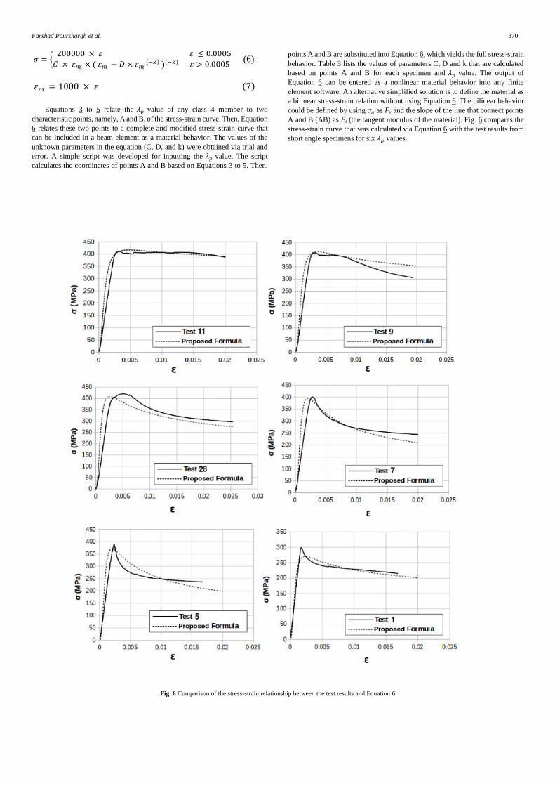
A and B (AB) as Et (the tangent modulus of the material). Fig. 6 compares the

stress-strain curve that was calculated via Equation 6 with the test results from

short angle specimens for six 𝜆𝑝 values.

Fig. 6 Comparison of the stress-strain relationship between the test results and Equation 6

Farshad Pourshargh et al. 371

Table 3

Calculated values of parameters for Equation 6

Tests 𝜆𝑝 C D k

1,2 1.13 440.289 0.563 1.272

3,4 1.05 526.022 0.625 1.329

5, 6, 18, 19, 20 1.01 563.891 0.653 1.346

7, 8 0.94 601.782 0.692 1.349

9, 10 0.62 512.091 0.831 1.123

11, 12 0.57 479.906 0.844 1.068

13, 14 0.86 602.713 0.729 1.315

15, 16 0.53 449.86 0.848 1.018

17 0.59 493.722 0.84 1.091

21 0.92 605.266 0.702 1.343

22 1.04 536.673 0.633 1.334

23, 25 0.63 517.363 0.827 1.133

24 0.48 441.128 0.847 1.004

26, 27 0.78 583.226 0.764 1.263

28 0.73 565.003 0.786 1.224

29, 30 0.75 572.487 0.777 1.24

31 0.61 506.351 0.834 1.113

32, 33 1.16 409.118 0.538 1.246

34 0.99 578.983 0.665 1.351

35, 36 0.79 585.562 0.76 1.269

37, 38 0.76 575.722 0.773 1.247

39, 40 0.64 523.266 0.824 1.143

41, 42 0.62 512.091 0.831 1.123

According to Fig. 6, the calculated curves are comparable to the

experimental results and they have an acceptable accuracy. This is also

demonstrated in Table 4, which compares the values of 𝜀𝐴, 𝜎𝐴 and 𝜎𝐵 from

Equation 6 and experimental work on short angles. The mean value of the

differences is very close to 1.0 and the COV values are reasonable for

parameters 𝜎𝐴 and 𝜎𝐵. The strain at the peak is always difficult to capture in

angles showing close to elasto-perfectly plastic behavior. As a consequence,

the COV value for parameter 𝜀𝐴 is relatively high. Despite the statistical

comparisons in Table 4, the trend of the stress-strain curve that was calculated

via the formula accords with the experimental results and the inaccuracy of

𝜀𝐴 does not impact the close agreement of the predicted curve with the

experimental results.

Table 4

Comparison of parameters that were calculated via Equation 6 with test values for parameters 𝜀𝐴, 𝜎𝐴, and 𝜎𝐵

Test 𝜀𝐴 (T) 𝜎𝐴 (T) 𝜎𝐵 (T) 𝜀𝐴 (F) 𝜎𝐴 (F) 𝜎𝐵 (F) 𝜀𝐴 (F/T) 𝜎𝐴 (F/T) 𝜎𝐵 (F/T)

1 0.0017 298 228 0.0021 317 234 1.24 1.06 1.03

2 0.0018 288 230 0.0021 317 234 1.17 1.1 1.02

3 0.0022 313 234 0.002 358 245 0.91 1.14 1.05

4 0.0035 297 242 0.002 358 245 0.57 1.21 1.01

5 0.0023 389 248 0.002 376 252 0.87 0.97 1.02

6 0.0021 379 250 0.002 376 252 0.95 0.99 1.01

7 0.0028 401 270 0.0019 397 269 0.68 0.99 1

8 0.0028 400 268 0.0019 397 269 0.68 0.99 1

9 0.0032 407 371 0.0036 412 383 1.13 1.01 1.03

10 0.0027 406 399 0.0036 412 383 1.33 1.01 0.96

11 0.0032 409 407 0.0046 416 402 1.44 1.02 0.99

12 0.0032 410 406 0.0046 416 402 1.44 1.01 0.99

13 0.0029 367 272 0.0022 406 291 0.76 1.11 1.07

Farshad Pourshargh et al. 372

14 0.0031 367 271 0.0022 406 291 0.71 1.11 1.07

15 0.0035 350 374 0.0042 418 428 1.2 1.2 1.14

16 0.0049 353 376 0.0042 418 428 0.86 1.19 1.14

17 0.0022 350 351 0.0042 414 397 1.91 1.18 1.13

18 0.0025 390 257 0.002 373 251 0.8 0.96 0.98

19 0.0026 384 255 0.002 376 252 0.77 0.98 0.99

20 0.0024 377 256 0.002 376 252 0.83 1 0.98

21 0.0024 371 254 0.0021 401 274 0.88 1.08 1.08

22 0.0022 356 242 0.0019 363 247 0.86 1.02 1.02

23 0.003 422 376 0.0034 411 379 1.13 0.97 1.01

24 0.005 423 437 0.0046 421 433 0.92 1 0.99

25 0.0035 425 392 0.0034 411 379 0.97 0.97 0.97

26 0.0034 413 305 0.0024 408 317 0.71 0.99 1.04

27 0.0032 413 302 0.0024 408 317 0.75 0.99 1.05

28 0.0048 420 357 0.0026 409 336 0.54 0.97 0.94

29 0.0036 414 332 0.0025 408 328 0.69 0.99 0.99

30 0.0035 413 334 0.0025 408 328 0.71 0.99 0.98

31 0.007 450 453 0.0038 412 388 0.54 0.92 0.86

32 0.0021 336 235 0.0021 302 231 1 0.9 0.98

33 0.0021 319 245 0.0021 302 231 1 0.95 0.94

34 0.0031 404 286 0.002 384 257 0.65 0.95 0.9

35 0.0029 418 293 0.0024 408 314 0.83 0.98 1.07

36 0.003 419 293 0.0024 408 314 0.8 0.97 1.07

37 0.0034 411 329 0.0025 408 323 0.74 0.99 0.98

38 0.0038 415 324 0.0025 408 323 0.66 0.98 1

39 0.0031 431 407 0.0033 411 374 1.06 0.95 0.92

40 0.0027 429 422 0.0033 411 374 1.22 0.96 0.89

41 0.003 432 427 0.0036 412 383 1.2 0.95 0.9

42 0.0031 429 424 0.0036 412 383 1.16 0.96 0.9

Average

0.93 1.02 1

COV (%)

30.29 7.56 6.53

Note: (T: Test, F: Formula) – The stress values are specified in MPa.

4. Evaluating the method with experimental results

4.1. Experimental Program

To evaluate the accuracy of the method, the numerical results were

compared to the results of experimental tests that were performed at

Université de Sherbrooke [24] on four X-bracing frame configurations. The

test setup is a two-dimensional frame than can include angle members that

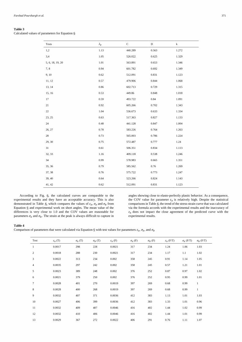
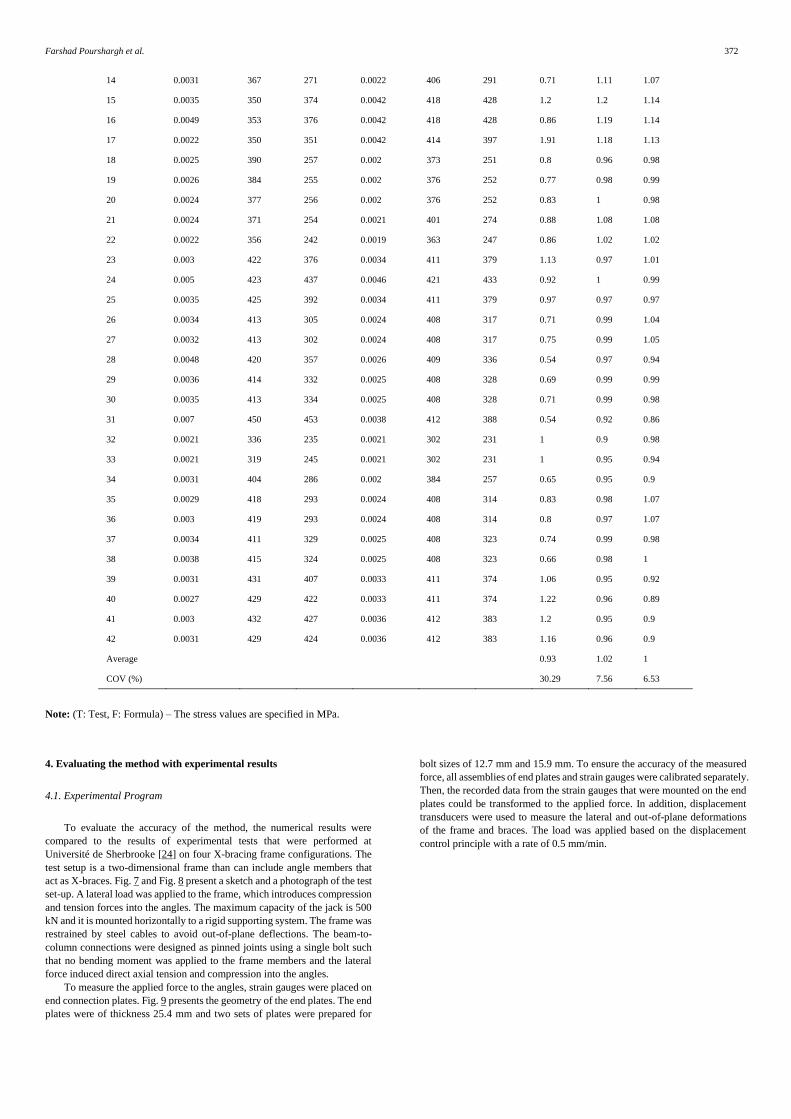
act as X-braces. Fig. 7 and Fig. 8 present a sketch and a photograph of the test

set-up. A lateral load was applied to the frame, which introduces compression

and tension forces into the angles. The maximum capacity of the jack is 500

kN and it is mounted horizontally to a rigid supporting system. The frame was

restrained by steel cables to avoid out-of-plane deflections. The beam-to-

column connections were designed as pinned joints using a single bolt such

that no bending moment was applied to the frame members and the lateral

force induced direct axial tension and compression into the angles.

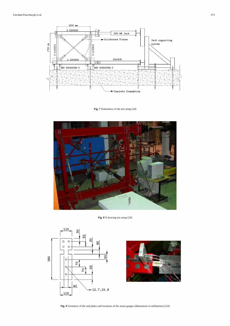
To measure the applied force to the angles, strain gauges were placed on

end connection plates. Fig. 9 presents the geometry of the end plates. The end

plates were of thickness 25.4 mm and two sets of plates were prepared for

bolt sizes of 12.7 mm and 15.9 mm. To ensure the accuracy of the measured

force, all assemblies of end plates and strain gauges were calibrated separately.

Then, the recorded data from the strain gauges that were mounted on the end

plates could be transformed to the applied force. In addition, displacement

transducers were used to measure the lateral and out-of-plane deformations

of the frame and braces. The load was applied based on the displacement

control principle with a rate of 0.5 mm/min.

Farshad Pourshargh et al. 373

Fig. 7 Schematics of the test setup [24]

Fig. 8 X-bracing test setup [24]

Fig. 9 Geometry of the end plates and locations of the strain gauges (dimensions in millimeters) [24]

Farshad Pourshargh et al. 374

4.2. Test Specimens

The X-bracing configuration involves two single angle sections under

tension and compression. The target member is the angle under compression.

Each angle is connected to the end plates using three bolts on one leg. The

same leg is restrained in the middle of the member by a single bolt that is

connected to the other bracing member, which is under tension. A filler plate

was provided to fit the space between two angles in the middle and to ensure

sufficient lateral support at the point of attachment (Fig. 10). The two

configurations were L38X38X3.2 and L44X44X3.2 angle sections. The

repeatability of results was assessed by testing two specimens for each

configuration. Table 5 lists the specimens and their properties, which are

based on tests that were conducted on coupons.

Fig. 10 Lateral support of the angles in the middle [24]

Table 5

Details of the X-bracing test specimens

Test Section D (mm) Fy (MPa)

1 L38X38X3.2 12.7 370

2 L38X38X3.2 12.7 392

3 L44X44X3.2 15.9 393

4 L44X44X3.2 15.9 393

Note: (D: Bolt diameter)

4.3. Finite Element Modeling of the Specimens

The four angle specimens of the previous section were modeled using the

Code_Aster software. Fiber beam elements are considered, and the optimum

element size was evaluated to be 100 mm after conducting preliminary tests.

To simplify the analysis, only the bracing angle members and the end

connection plates are included in the model. A preliminary deflection value

of Length/1000 [30] at the mid-length of the braces is applied to the weak

bending axis as a global geometrical imperfection. It is assumed that the

outside frame members are rigid in comparison to the angle members.

Therefore, the end connection plates on top are supported by fixed supports

with only unrestrained lateral displacement. The bottom supports are assumed

to be fixed. The angle members are connected to these supports via two

elements: a rigid beam element, which is used to include the member

eccentricity, and a nonlinear spring, which is used to model the three-bolt-

connection behavior. The properties of the spring element depend on the

slippage and the bolted connection behavior according to the formulas that

are presented by Rex et al. [33]. To model the single bolt that attaches the

members at the middle of the bracing system, it is assumed that the middle

nodes have identical displacement. However, the relative rotational

displacement is free at this point.

The proposed method was applied to the analysis. First, 𝜎𝑐𝑟 was

calculated for each specimen using Code_Aster (Fig. 11). Since the boundary

conditions of the members are not as described in Section 2.1, Equation 2

cannot be used and finite element modeling is implemented instead. In the X-

bracing tests, the angle member needed to be restrained at the middle for

modeling the pinned connection. Since CUFSM could not apply this type of

restraint to the member, Code_Aster was used to perform the calculation. The

bracing member under compression was modeled in Code_Aster using plate

elements and mesh refinement was optimized via several trials. Each element

had four corner nodes with six degrees of freedom and the maximum element

size was 4 mm. Fixed boundary conditions were applied to the nodes on one

leg of the member on each end. To model the constraint in the middle of the

brace member, a hinged support was applied to a node on the same supported

leg (Fig. 7). Then, the elastic buckling analysis was performed and the 𝜎𝑐𝑟

value was calculated for the brace member.

The next step was to calculate the 𝜆𝑝 value for each specimen via

Equation 1. Table 6 summarizes the calculated 𝜎𝑐𝑟 and 𝜆𝑝 values for each

specimen. Then, the stress-strain curve is calculated using the two steps that

were specified earlier: first, Equations 3 to 5 were used to calculate two points,

namely, A and B, on the curve for the specified value of 𝜆𝑝; second, the

parameters in Equations 6 and 7 were calculated such that the stress-strain

curve passes through points A and B. In the final step, the calculated curve is

applied as a material behavior to the fiber elements of the specimens. The

nonlinear analysis phase is completed by Code_Aster and the assumptions of

nonlinear material and large displacements are included in the procedure.

Fig. 11 Local buckling mode of a specimen (Test 3)

Table 6

Calculated 𝜎𝑐𝑟 and 𝜆𝑝 values for the test specimens

4.4. Results comparison and discussion

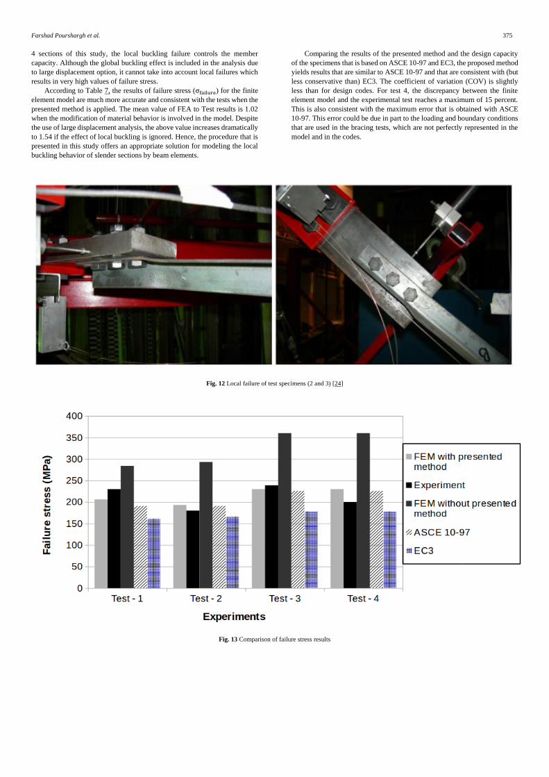
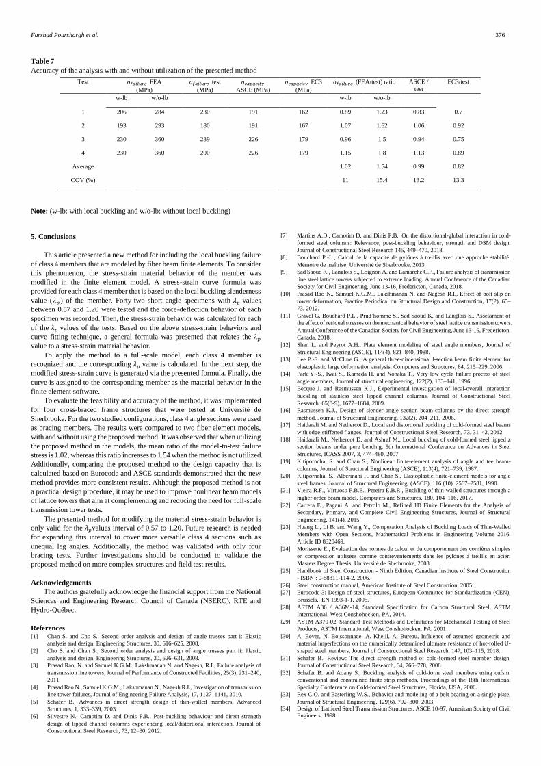
The experimental specimens failed due to local buckling phenomena. Fig.

12 shows the final deflection for four of the test specimens. Fig. 13 compares

the failure stresses of the experimental tests to those of the finite element

models and the member capacity based on ASCE 10-97 [34] and EC3 [27].

To evaluate the performance of the presented method, another set of analyses

is performed without applying the proposed method to account for local

buckling in the model. According to the comparisons, neglecting the local

buckling failure in the analysis results in very high failure stresses. In the class

Test 𝜎𝑐𝑟

(MPa)

𝜆𝑝

1 295 1.11

2 295 1.15

3 234 1.29

4 234 1.29

Farshad Pourshargh et al. 375 4 sections of this study, the local buckling failure controls the member

capacity. Although the global buckling effect is included in the analysis due

to large displacement option, it cannot take into account local failures which

results in very high values of failure stress.

According to Table 7, the results of failure stress (σfailure) for the finite

element model are much more accurate and consistent with the tests when the

presented method is applied. The mean value of FEA to Test results is 1.02

when the modification of material behavior is involved in the model. Despite

the use of large displacement analysis, the above value increases dramatically

to 1.54 if the effect of local buckling is ignored. Hence, the procedure that is

presented in this study offers an appropriate solution for modeling the local

buckling behavior of slender sections by beam elements.

Comparing the results of the presented method and the design capacity

of the specimens that is based on ASCE 10-97 and EC3, the proposed method

yields results that are similar to ASCE 10-97 and that are consistent with (but

less conservative than) EC3. The coefficient of variation (COV) is slightly

less than for design codes. For test 4, the discrepancy between the finite

element model and the experimental test reaches a maximum of 15 percent.

This is also consistent with the maximum error that is obtained with ASCE

10-97. This error could be due in part to the loading and boundary conditions

that are used in the bracing tests, which are not perfectly represented in the

model and in the codes.

Fig. 12 Local failure of test specimens (2 and 3) [24]

Fig. 13 Comparison of failure stress results

Farshad Pourshargh et al. 376

Table 7

Accuracy of the analysis with and without utilization of the presented method

Note: (w-lb: with local buckling and w/o-lb: without local buckling)

5. Conclusions

This article presented a new method for including the local buckling failure

of class 4 members that are modeled by fiber beam finite elements. To consider

this phenomenon, the stress-strain material behavior of the member was

modified in the finite element model. A stress-strain curve formula was

provided for each class 4 member that is based on the local buckling slenderness

value (𝜆𝑝 ) of the member. Forty-two short angle specimens with 𝜆𝑝 values

between 0.57 and 1.20 were tested and the force-deflection behavior of each

specimen was recorded. Then, the stress-strain behavior was calculated for each

of the 𝜆𝑝 values of the tests. Based on the above stress-strain behaviors and

curve fitting technique, a general formula was presented that relates the 𝜆𝑝

value to a stress-strain material behavior.

To apply the method to a full-scale model, each class 4 member is

recognized and the corresponding 𝜆𝑝 value is calculated. In the next step, the

modified stress-strain curve is generated via the presented formula. Finally, the

curve is assigned to the corresponding member as the material behavior in the

finite element software.

To evaluate the feasibility and accuracy of the method, it was implemented

for four cross-braced frame structures that were tested at Université de

Sherbrooke. For the two studied configurations, class 4 angle sections were used

as bracing members. The results were compared to two fiber element models,

with and without using the proposed method. It was observed that when utilizing

the proposed method in the models, the mean ratio of the model-to-test failure

stress is 1.02, whereas this ratio increases to 1.54 when the method is not utilized.

Additionally, comparing the proposed method to the design capacity that is

calculated based on Eurocode and ASCE standards demonstrated that the new

method provides more consistent results. Although the proposed method is not

a practical design procedure, it may be used to improve nonlinear beam models

of lattice towers that aim at complementing and reducing the need for full-scale

transmission tower tests.

The presented method for modifying the material stress-strain behavior is

only valid for the 𝜆𝑝values interval of 0.57 to 1.20. Future research is needed

for expanding this interval to cover more versatile class 4 sections such as

unequal leg angles. Additionally, the method was validated with only four

bracing tests. Further investigations should be conducted to validate the

proposed method on more complex structures and field test results.

Acknowledgements

The authors gratefully acknowledge the financial support from the National

Sciences and Engineering Research Council of Canada (NSERC), RTE and

Hydro-Québec.

References [1] Chan S. and Cho S., Second order analysis and design of angle trusses part i: Elastic

analysis and design, Engineering Structures, 30, 616–625, 2008.

[2] Cho S. and Chan S., Second order analysis and design of angle trusses part ii: Plastic

analysis and design, Engineering Structures, 30, 626–631, 2008.

[3] Prasad Rao, N. and Samuel K.G.M., Lakshmanan N. and Nagesh, R.I., Failure analysis of

transmission line towers, Journal of Performance of Constructed Facilities, 25(3), 231–240,

2011.

[4] Prasad Rao N., Samuel K.G.M., Lakshmanan N., Nagesh R.I., Investigation of transmission

line tower failures, Journal of Engineering Failure Analysis, 17, 1127–1141, 2010.

[5] Schafer B., Advances in direct strength design of thin-walled members, Advanced

Structures, 1, 333–339, 2003.

[6] Silvestre N., Camotim D. and Dinis P.B., Post-buckling behaviour and direct strength

design of lipped channel columns experiencing local/distortional interaction, Journal of

Constructional Steel Research, 73, 12–30, 2012.

[7] Martins A.D., Camotim D. and Dinis P.B., On the distortional-global interaction in cold-

formed steel columns: Relevance, post-buckling behaviour, strength and DSM design,

Journal of Constructional Steel Research 145, 449–470, 2018.

[8] Bouchard P.-L., Calcul de la capacité de pylônes à treillis avec une approche stabilité.

Mémoire de maîtrise. Université de Sherbrooke, 2013.

[9] Sad Saoud K., Langlois S., Loignon A. and Lamarche C.P., Failure analysis of transmission

line steel lattice towers subjected to extreme loading. Annual Conference of the Canadian

Society for Civil Engineering, June 13-16, Fredericton, Canada, 2018.

[10] Prasad Rao N., Samuel K.G.M., Lakshmanan N. and Nagesh R.I., Effect of bolt slip on

tower deformation, Practice Periodical on Structural Design and Construction, 17(2), 65–

73, 2012.

[11] Gravel G, Bouchard P.L., Prud’homme S., Sad Saoud K. and Langlois S., Assessment of

the effect of residual stresses on the mechanical behavior of steel lattice transmission towers.

Annual Conference of the Canadian Society for Civil Engineering, June 13-16, Fredericton,

Canada, 2018.

[12] Shan L. and Peyrot A.H., Plate element modeling of steel angle members, Journal of

Structural Engineering (ASCE), 114(4), 821–840, 1988.

[13] Lee P.-S. and McClure G., A general three-dimensional l-section beam finite element for

elastoplastic large deformation analysis, Computers and Structures, 84, 215–229, 2006.

[14] Park Y.-S., Iwai S., Kameda H. and Nonaka T., Very low cycle failure process of steel

angle members, Journal of structural engineering, 122(2), 133–141, 1996.

[15] Becque J. and Rasmussen K.J., Experimental investigation of local-overall interaction

buckling of stainless steel lipped channel columns, Journal of Constructional Steel

Research, 65(8-9), 1677–1684, 2009.

[16] Rasmussen K.J., Design of slender angle section beam-columns by the direct strength

method, Journal of Structural Engineering, 132(2), 204–211, 2006.

[17] Haidarali M. and Nethercot D., Local and distortional buckling of cold-formed steel beams

with edge-stiffened flanges, Journal of Constructional Steel Research, 73, 31–42, 2012.

[18] Haidarali M., Nethercot D. and Ashraf M., Local buckling of cold-formed steel lipped z

section beams under pure bending, 5th International Conference on Advances in Steel

Structures, ICASS 2007, 3, 474–480, 2007.

[19] Kitipornchai S. and Chan S., Nonlinear finite-element analysis of angle and tee beam-

columns, Journal of Structural Engineering (ASCE), 113(4), 721–739, 1987.

[20] Kitipornchai S., Albermani F. and Chan S., Elastoplastic finite-element models for angle

steel frames, Journal of Structural Engineering, (ASCE), 116 (10), 2567–2581, 1990.

[21] Vieira R.F., Virtuoso F.B.E., Pereira E.B.R., Buckling of thin-walled structures through a

higher order beam model, Computers and Structures, 180, 104–116, 2017.

[22] Carrera E., Pagani A. and Petrolo M., Refined 1D Finite Elements for the Analysis of

Secondary, Primary, and Complete Civil Engineering Structures, Journal of Structural

Engineering, 141(4), 2015.

[23] Huang L., Li B. and Wang Y., Computation Analysis of Buckling Loads of Thin-Walled

Members with Open Sections, Mathematical Problems in Engineering Volume 2016,

Article ID 8320469.

[24] Morissette E., Évaluation des normes de calcul et du comportement des cornières simples

en compression utilisées comme contreventements dans les pylônes à treillis en acier,

Masters Degree Thesis, Université de Sherbrooke, 2008.

[25] Handbook of Steel Construction - Ninth Edition, Canadian Institute of Steel Construction

- ISBN : 0-88811-114-2, 2006.

[26] Steel construction manual, American Institute of Steel Construction, 2005.

[27] Eurocode 3: Design of steel structures, European Committee for Standardization (CEN),

Brussels., EN 1993-1-1, 2005.

[28] ASTM A36 / A36M-14, Standard Specification for Carbon Structural Steel, ASTM

International, West Conshohocken, PA, 2014.

[29] ASTM A370-02, Standard Test Methods and Definitions for Mechanical Testing of Steel

Products, ASTM International, West Conshohocken, PA, 2001

[30] A. Beyer, N. Boissonnade, A. Khelil, A. Bureau, Influence of assumed geometric and

material imperfections on the numerically determined ultimate resistance of hot-rolled U-

shaped steel members, Journal of Constructional Steel Research, 147, 103–115, 2018.

[31] Schafer B., Review: The direct strength method of cold-formed steel member design,

Journal of Constructional Steel Research, 64, 766–778, 2008.

[32] Schafer B. and Adany S., Buckling analysis of cold-form steel members using cufsm:

conventional and constrained finite strip methods, Proceedings of the 18th International

Specialty Conference on Cold-formed Steel Structures, Florida, USA, 2006.

[33] Rex C.O. and Easterling W.S., Behavior and modeling of a bolt bearing on a single plate,

Journal of Structural Engineering, 129(6), 792–800, 2003.

[34] Design of Latticed Steel Transmission Structures. ASCE 10-97, American Society of Civil

Engineers, 1998.

Test 𝜎𝑓𝑎𝑖𝑙𝑢𝑟𝑒 FEA

(MPa)

𝜎𝑓𝑎𝑖𝑙𝑢𝑟𝑒 test

(MPa)

𝜎𝑐𝑎𝑝𝑎𝑐𝑖𝑡𝑦

ASCE (MPa)

𝜎𝑐𝑎𝑝𝑎𝑐𝑖𝑡𝑦 EC3

(MPa)

𝜎𝑓𝑎𝑖𝑙𝑢𝑟𝑒 (FEA/test) ratio ASCE /

test

EC3/test

w-lb w/o-lb

w-lb w/o-lb

1 206 284 230 191 162 0.89 1.23 0.83 0.7

2 193 293 180 191 167 1.07 1.62 1.06 0.92

3 230 360 239 226 179 0.96 1.5 0.94 0.75

4 230 360 200 226 179 1.15 1.8 1.13 0.89

Average

1.02 1.54 0.99 0.82

COV (%)

11 15.4 13.2 13.3