Modeling quasi-static crack growth with the extended ﬁnite element ...dilbert.engr.ucdavis.edu/~suku/xfem/papers/xfem_partI.pdf · and the crack path are outcomes of the analysis

International Journal of Solids and Structures 40 (2003) 7513–7537

www.elsevier.com/locate/ijsolstr

Modeling quasi-static crack growthwith the extended finite element method

Part I: Computer implementation

N. Sukumar a,*, J.-H. Preevost b

a Department of Civil and Environmental Engineering, University of California, One Shields Avenue, Davis, CA 95616, USAb Department of Civil and Environmental Engineering, Princeton University, Princeton, NJ 08544, USA

Received 30 October 2002; received in revised form 30 May 2003

Abstract

The extended finite element method (X-FEM) is a numerical method for modeling strong (displacement) as well as

weak (strain) discontinuities within a standard finite element framework. In the X-FEM, special functions are added to

the finite element approximation using the framework of partition of unity. For crack modeling in isotropic linear

elasticity, a discontinuous function and the two-dimensional asymptotic crack-tip displacement fields are used to ac-

count for the crack. This enables the domain to be modeled by finite elements without explicitly meshing the crack

surfaces, and hence quasi-static crack propagation simulations can be carried out without remeshing. In this paper, we

discuss some of the key issues in the X-FEM and describe its implementation within a general-purpose finite element

code. The finite element program Dynaflowe is considered in this study and the implementation for modeling 2-d

cracks in isotropic and bimaterial media is described. In particular, the array-allocation for enriched degrees of free-

dom, use of geometric-based queries for carrying out nodal enrichment and mesh partitioning, and the assembly

procedure for the discrete equations are presented. We place particular emphasis on the design of a computer code to

enable the modeling of discontinuous phenomena within a finite element framework.

2003 Elsevier Ltd. All rights reserved.

Keywords: Strong discontinuities; Partition of unity; Extended finite element; Finite element programming; Crack modeling;

Singularity

1. Introduction

A problem of significant interest and importance in solid mechanics is the modeling of fracture and

damage phenomena. These material failure processes manifest themselves in quasi-brittle materials such as

rocks and concrete as fracture process zones, shear (localization) bands in ductile metals, or discrete crack

discontinuities in brittle materials. The accurate modeling and the evolution of smeared and discrete

* Corresponding author. Tel.: +1-530-7546415; fax: +1-530-7527872.

E-mail address: [email protected] (N. Sukumar).

0020-7683/$ - see front matter 2003 Elsevier Ltd. All rights reserved.

doi:10.1016/j.ijsolstr.2003.08.002

mail to: [email protected]

7514 N. Sukumar, J.-H. Preevost / International Journal of Solids and Structures 40 (2003) 7513–7537

discontinuities has been a topic of growing interest over the past few decades, with quite a few notable

developments in computational techniques over the past few years.

Early numerical models for treating discontinuities in finite elements can be traced to the work of Ortiz

et al. (1987) and Belytschko et al. (1988). They modeled shear bands as weak (strain) discontinuities thatcould pass through finite elements using a multi-field variational principle. Dvorkin et al. (1990) con-

sidered strong (displacement) discontinuities by modifying the principle of virtual work statement,

whereas Lotfi and Sheng (1995) extended the three-field Hu–Washizu variational statement for bodies

with internal discontinuities. A unified framework for analyzing strong discontinuities by taking into

account the softening constitutive law and the interface traction–displacement relation was put forth by

Simo and co-workers (Simo et al., 1993; Simo and Oliver, 1994). Applications and extensions of this

approach have been proposed by many researchers for pre- as well as post-localization analyses (Armero

and Garikipati, 1996; Sluys and Berends, 1998; Larsson and Runesson, 1996; Larsson et al., 1999;Regueiro and Borja, 2001; Bolzon and Corigliano, 2000). Borja (2000) presented a standard Galerkin

formulation of the strong discontinuity approach and has shown its equivalence to assumed enhanced

strain approximations.

In the strong discontinuity approach, the displacement consists of regular and enhanced components,

where the enhanced component yields a jump across the discontinuity surface. An assumed enhanced strain

variational formulation is used, and the enriched degrees of freedom are statically condensed on an element

level to obtain the tangent stiffness matrix for the element. A comprehensive review and comparison of

various embedded discontinuity approaches is provided by Jiraasek (2000). An alternative approach tomodeling fracture phenomena is the cohesive surface formulation of Xu and Needleman (1994), which has

been used to model damage in brittle materials (Camacho and Ortiz, 1996). The cohesive surface formu-

lation is a phenomenological framework in which the fracture characteristics of the material are embedded

in a cohesive surface traction–displacement relation. Using this approach, an inherent length scale is in-

troduced into the model, and in addition no fracture criterion (K-dominant field) is required; crack growth

and the crack path are outcomes of the analysis.

A significant improvement in crack modeling was realized with the development of a partition-of-unity

based enrichment method for discontinuous fields (Mo€ees et al., 1999), which was referred to as the ex-tended finite element method (X-FEM) (Dolbow, 1999; Daux et al., 2000). In the X-FEM, special

functions are added to the finite element approximation using the framework of partition of unity (Melenk

and Babusska, 1996; Duarte and Oden, 1996). For crack modeling, a discontinuous function (generalized

Heaviside step function) and the two-dimensional linear elastic asymptotic crack-tip displacement fields

are used to account for the crack. This enables the domain to be modeled by finite elements without

explicitly meshing the crack surfaces. The location of the crack discontinuity can be arbitrary with respect

to the underlying finite element mesh, and quasi-static or fatigue crack propagation simulations can be

performed without the need to remesh as the crack advances. A particularly appealing feature is that thefinite element framework and its properties (sparsity and symmetry) are retained, and a single-field

(displacement) variational principle is used to obtain the discrete equations. This technique provides an

accurate and robust numerical method to model strong (displacement) discontinuities in 2-d (Mo€ees et al.,1999; Daux et al., 2000) and 3-d (Sukumar et al., 2000), as well as weak (strain) discontinuities (Sukumar

et al., 2001).

In this paper, we describe the main issues in the implementation of the X-FEM, and present a robust and

simple means to incorporate it into a general-purpose finite element program. The finite element program

Dynaflowe (Preevost, 1983) is considered in this study and the methodology for modeling 2-d cracks inisotropic and bimaterial media is presented. The initial development of the X-FEM at Northwestern

University and the many recent advances of the method have all been carried out within a C++ code.

However, since most existing finite element codes are in Fortran, we undertake the task to outline the X-

FEM implementation within such a programming environment. The main contributions in this paper are:

N. Sukumar, J.-H. Preevost / International Journal of Solids and Structures 40 (2003) 7513–7537 7515

• To provide a detailed account of the main issues that arise in the implementation of the X-FEM, and

how to incorporate them within an existing finite element code so that apart from crack modeling,

the incorporation of other types of discontinuities will also become apparent.

• Design of data structures for variable nodal degrees of freedom array and for the assembly of the discreteequations. The computational algorithms to select the enriched nodes and to compute the enrichment

functions are described. The need for partitioning of elements is addressed, and its distinction from reme-

shing is pointed out.

• Step-by-step treatment of the assembly procedure of the bilinear form for elements that are cut by the

crack; this aspect has not been described in earlier works. In addition, details on the submatrices and

vectors that arise in the global stiffness matrix and external force vector are provided.

In Section 2, the extended finite element method is introduced and recent applications of the method inmechanics and materials science are mentioned. Crack modeling in the X-FEM is discussed in Section 2.1.

The implementation of the X-FEM within Dynaflowe is outlined in Section 3, and a few concluding

remarks are made in Section 4.

2. Extended finite element method

The partition of unity method (Melenk and Babusska, 1996; Duarte and Oden, 1996) generalized finite

element approximations by presenting a means to embed local solutions of boundary-value problems into

the finite element approximation. This idea was first exploited by Oden and co-workers (Oden et al., 1998;

Duarte et al., 1998) for problems with internal boundaries––the numerical technique was termed as the

generalized finite element method (GFEM). Strouboulis et al. (2000) used local enrichment functions in the

GFEM for modeling re-entrant corners and holes, whereas Duarte et al. (2001) simulated dynamic crackpropagation in 3-d using the partition of unity framework. A comprehensive summary of the GFEM

appears in Strouboulis et al. (2001).

In Belytschko and Black (1999), the partition of unity enrichment for crack discontinuities and near-tip

crack fields was introduced. The enrichment functions for crack problems are functions that span the as-

ymptotic near-tip displacement field––see Fleming et al. (1997) for their use in the element-free Galerkin

method (Belytschko et al., 1994). A notable improvement and progress in discrete crack growth modeling

without the need for any remeshing strategy was conceived in Mo€ees et al. (1999). The generalized Heaviside

function was proposed as a means to model the crack away from the crack-tip, with simple rules for theintroduction of the discontinuous and crack-tip enrichments. This advance has provided a robust and

accurate computational tool for modeling discontinuities independent of the crack geometry. The partition

of unity framework satisfies a few key properties which renders it as a powerful tool for local enrichment

within a finite element setting:

1. can include application-specific basis functions to better approximate the solution;

2. automatic enforcement of continuity (conforming trial and test approximations); and

3. point or line singularities as well as surface discontinuities can be handled without the need for the dis-

continuous surfaces to be aligned with the finite element mesh.

The above properties are in sharp contrast to enriched finite elements (Benzley, 1974; Gifford and Hilton,

1978; Ayhan and Nied, 2002), where transition elements are required to satisfy displacement continuity. In

classical as well as enriched finite element methods, remeshing is required to conduct crack growth simu-

lations.


The X-FEM has been successfully applied to 2-dimensional static and quasi-static crack growth prob-

lems (Mo€ees et al., 1999; Dolbow, 1999; Dolbow et al., 2000a,b; Dolbow et al., 2001; Mo€ees and Belytschko,

2002), with its extension to modeling holes, and branched and intersecting cracks proposed in Daux et al.

(2000). The application of this technique for 3-dimensional crack problems was presented in Sukumar et al.(2000). The interface of the X-FEM with level set techniques to model weak discontinuities such as material

interfaces (bimaterials) was introduced in Sukumar et al. (2001), whereas the representation of tangential

discontinuities was presented in Belytschko et al. (2001). Recent studies have explored the use of fast

marching and level sets for evolving crack discontinuities in 2-dimensions (Stolarska et al., 2001) and 3-

dimensions within the X-FEM framework. The growth of multiple coplanar cracks in 3-d is handled using

the fast marching method (Sukumar et al., 2003a; Chopp and Sukumar, 2003), whereas non-planar crack

growth is carried out using level sets (Mo€ees et al., 2002; Gravouil et al., 2002).

The X-FEM has also been utilized to model computational phenomena in areas such as fluid mechanics,phase transformations, and materials science. In Wagner et al. (2001), a computational model for rigid

particles in Stokes flow was proposed, whereas moving phase boundary problems have been modeled using

the coupled extended finite element and level set methods (Merle and Dolbow, 2002; Ji et al., 2002; Chessa

et al., 2002). Dolbow and Nadeau (2002) investigated the use of effective properties for fracture analysis in

functionally-graded systems, whereas Sukumar et al. (2003b) adopted the X-FEM as a fracture tool to

study the competition between intergranular and transgranular modes of crack growth through a material

microstructure. In other related studies, Wells and Sluys (2001) used the Heaviside step function to model

the displacement discontinuity within a finite-element based cohesive crack model, whereas Wells et al.(2002) used partition of unity enrichment to alleviate volumetric locking during plastic flow.

2.1. Crack modeling in two-dimensions

In finite elements, a basis function NI is associated with node I in the mesh. Let xI ¼ fx : NIðxÞ > 0g be

the region of support for NI . The nodes belonging to an element are given by the connectivity of the ele-

ment, whereas its dual xI , is the collection of elements that are associated with a specific node I (see Fig. 1).In the X-FEM, a crack is represented by enriching the classical displacement-based finite element ap-

proximation through the framework of partition of unity (Melenk and Babusska, 1996). A crack is modeled

by enriching the nodes whose nodal shape function support intersects the interior of the crack by a dis-

continuous function, and enriching the nodes whose nodal shape function supports intersect the crack-tip

by the two-dimensional linear elastic asymptotic near-tip fields. Additional degrees of freedom are asso-ciated with nodes that are enriched. Partitioning algorithms are also implemented if the crack intersects the

finite elements. We first present the enrichment functions used for crack modeling and the criteria for the

selection of the enriched nodes. Then, the need for element partitioning is discussed and lastly, the discrete

equations are presented.

Fig. 1. Support xI (dark line) for a nodal shape function.


2.1.1. Enrichment functions

We will use lower case and upper case bold-faced letters to denote vectors and matrices, respectively. The

Cartesian coordinate axes are denoted by x ðx; yÞ in 2-d, with Latin lower case indices referring to

Cartesian components. Nodes in the finite element mesh are denoted by Latin subscripts––lower case in-dices refer to the local node number within an element whereas upper case indices are used for the global

node number in the mesh (Hughes, 1987). Consider a body X R2 that contains an internal traction-free

crack (Fig. 2). For a single crack in 2-dimensions, let Cc be the crack surface (interior) and Kc the crack

tip(s)––the closure Cc ¼ Cc [ Kc. The description of the enrichment functions follows:

Generalized Heaviside function. The interior of a crack (Cc is the enrichment-domain) is modeled by the

generalized Heaviside enrichment function H , where H takes on the value +1 above the crack and )1 below

the crack (Mo€ees et al., 1999):

HðxÞ ¼ 1 if ðx xÞ nP 0;1 otherwise;

ð1Þ

where x is a sample (Gauss) point, x (lies on the crack) is the closest point to x, and n is the unit outward

normal to the crack at x.

Near-tip crack functions. To model the crack-tip and also to improve the representation of crack-tip

fields in fracture computations, crack-tip enrichment functions are used in the element which contains the

crack tip. The crack-tip enrichment consists of functions which incorporate the radial and angular behavior

of the two-dimensional asymptotic crack-tip displacement field. The use of the crack-tip functions serves

two main purposes:

1. If the crack were to terminate in the interior of an element, then enriching the crack-tip element with the

Heaviside function would be inaccurate. This is so, since by such a choice the crack would be modeled as

though the segment containing the crack-tip were extended till it intersected the element edge. The crack-

tip enrichment functions ensure that the crack terminates precisely at the location of the crack-tip, and

hence these functions are required to model the crack for this case.

2. The use of the linear elastic (or bimaterial) asymptotic crack-tip fields serve as suitable enrichment func-

tions for they possess the correct near-tip behavior, and in addition, their use also leads to better accu-

racy on relatively coarse finite element meshes in 2-d (Mo€ees et al., 1999; Daux et al., 2000; Huang et al.,2003a,b; Sukumar et al., 2003a) and 3-d (Sukumar et al., 2000).

The crack-tip enrichment functions in isotropic elasticity are (Fleming et al., 1997):

½UaðxÞ; a ¼ 1–4 ¼ffiffir

psin

h2;ffiffir

pcos

h2;ffiffir

psin h sin

h2;ffiffir

psin h cos

h2

; ð2Þ

c

c

t

u

t

Ω

+ ΓΓ

ΓΓ

Fig. 2. Boundary value problem with an internal traction-free crack.


where r and h are polar coordinates in the local crack-tip coordinate system. Note that the first function in

the above equation is discontinuous across the crack. In Fig. 3, the shape function support xI as well as the

local coordinate system for the crack-tip enrichment functions are illustrated.

The use of crack-tip functions is not restricted to crack modeling in isotropic media alone. Consider abimaterial with a crack perpendicular to the interface (Fig. 4); the crack terminates at the interface. The

near-tip asymptotic field for this problem has been studied by many researchers (Zak and Williams, 1963;

Bogy, 1971; Cook and Erdogan, 1972; Chen, 1994). The elastic mismatch between the two elastic materials

is characterized by Dundurs parameters (Dundurs, 1969):

a ¼ l1ðj2 þ 1Þ l2ðj1 þ 1Þl1ðj2 þ 1Þ þ l2ðj1 þ 1Þ ; b ¼ l1ðj2 1Þ l2ðj1 1Þ

l1ðj2 þ 1Þ þ l2ðj1 þ 1Þ ; ð3aÞ

ji ¼3 mi1þ mi

ðplane stressÞ;3 4mi ðplane strainÞ;

8<: ð3bÞ

where li and mi are the shear modulus and the Poissons ratio, respectively, of material i (i ¼ 1; 2).The asymptotic displacement field near the tip of a plane strain crack in a bimaterial takes the form

(Chen, 1994)

uiðr; hÞ ¼ r1k ai sin khf þ bi cos khþ ci sinðk 2Þhþ di cosðk 2Þhg; ð4Þ

where k (0 < k < 1), which is the stress singularity exponent, is a function of the Dundurs parameters and is

given by the root of the transcendental equation (Zak and Williams, 1963)

rCRACK

ωΙ

I

θ

Fig. 3. Coordinate configuration ðr; hÞ for crack tip enrichment functions.

h1

h2

E ,1 ν1

E ,2 ν2

Material 1

Material 2

crack

Fig. 4. Bimaterial with a crack impinging on the interface.


cosðkpÞ 2a b1 b

ð1 kÞ2 þ a b2

1 b2¼ 0: ð5Þ

The value of k as a function of a and b is tabulated in Beuth (1992). In the case of no mismatch (a ¼ b ¼ 0),

the stress singularity reduces to the classical inverseffiffir

pstress singularity (k ¼ 1=2) for homogeneous linear

elastic materials. When material 2 is stiffer than material 1 (a < 0), the singularity is weaker (k < 1=2), andif material 2 is more compliant than material 1 (a > 0), the singularity is stronger (k > 1=2).

The crack-tip enrichment functions for the bimaterial crack problem are (Huang et al., 2003a,b):

½WaðxÞ; a ¼ 1–4 ¼ r1k sin kh; r1k cos kh; r1k sinðk

2Þh; r1k cosðk 2Þh; ð6Þ

where the above functions span the asymptotic crack-tip displacement expansion given in Eq. (4). Note that

in this instance the first function and the third function in the above equation are discontinuous across the

crack (h ¼ p). Recently, partition of unity enrichment for modeling bimaterial interface cracks has alsobeen developed within Dynaflowe; see Sukumar et al. (in press) for details.

2.1.2. Selection of enriched nodes

The approximation for a vector-valued function u with the partition of unity enrichment is of the general

form (Melenk and Babusska, 1996):

uhðxÞ ¼XNI¼1

NIðxÞXMa¼1

waðxÞaaI

!; ð7Þ

where NI are the finite element shape functions and wa are the enrichment functions. The finite elementshape functions form a partition of unity:

PI NIðxÞ ¼ 1. From Eq. (7), we note that the finite element space

(w1 1; wa ¼ 0 ða 6¼ 1Þ) is a subspace of the enriched space.

In the particular instance of 2-d crack modeling, the enriched displacement (trial and test) approxi-

mation is written as (Mo€ees et al., 1999):

uhðxÞ ¼XI2N

NIðxÞ uI

26664 þ HðxÞaI|fflfflfflzfflfflffl

I2NC

þX4a¼1

UaðxÞbaI|fflfflfflfflfflfflfflfflzfflfflfflfflfflfflfflfflI2NK

37775; ð8Þ

where uI is the nodal displacement vector associated with the continuous part of the finite element solution,

aI is the nodal enriched degree of freedom vector associated with the Heaviside (discontinuous) function,

and baI is the nodal enriched degree of freedom vector associated with the elastic asymptotic crack-tip

functions. In the above equation, N is the set of all nodes in the mesh; NC is the set of nodes whose shape

function support is cut by the crack interior Cc; and NK is the set of nodes whose shape function support is

cut by the crack tip Kc (NC \NK ¼ ;):
NK ¼ fnK : nK 2 N; xxK \ Kc 6¼ ;g; ð9aÞ
NC ¼ fnJ : nJ 2 N;xJ \ Cc 6¼ ;; nJ 62 NKg: ð9bÞ
For any node in NC, the support of the nodal shape function is fully cut into two disjoint pieces by the
crack. If for a certain node nI , one of the two pieces is very small compared to the other, then the gene-

ralized Heaviside function used for the enrichment is almost a constant over the support, leading to an ill-

conditioned stiffness matrix (Mo€ees et al., 1999). Therefore, in this case, node nI is removed from the setNK.The area-criterion for nodal inclusion in NK is as follows: The area above the crack is Aabove

x , and the area

below the crack is Abelowx : Ax ¼ Aabove

x þ Abelowx . If either of the two ratios, Aabove

x =Ax or Abelowx =Ax is below a

crack-tip

crack-tip

(a) (b)

(c) (d)

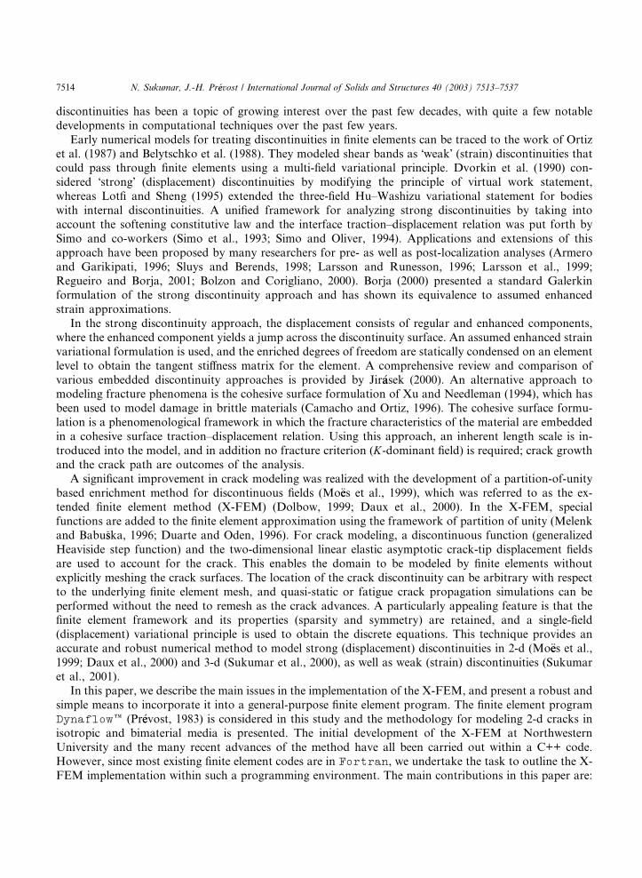
Fig. 5. Heaviside and near-tip nodal enrichment for a 2-d edge-crack problem. The Heaviside enriched nodes are shown in filled circles,

the near-tip enriched nodes are shown in open circles, and the enrichment region can be inferred from the contour plot, where the

contour value on an enriched node is unity and zero on all other nodes. (a) Heaviside enrichment for regular (rectangular) mesh;

(b) Near-tip enrichment for regular (rectangular) mesh; (c) Heaviside enrichment for unstructured (triangular) mesh; and (d) Near-

tip enrichment for unstructured (triangular) mesh.


prescribed tolerance, the node is removed from the set NK (Dolbow et al., 2000a). A tolerance ¼ 104 is

used in the computations.The enriched nodes for the interior of a crack and those for the crack tip are shown in Fig. 5. From the

contours shown in Fig. 5, one can also infer the region (union of elements) over which the enriched basis

functions are non-zero.

2.1.3. Element partitioning versus remeshing

If a crack intersects an element, the element is subdivided into triangles (in 2-d) such that element edges

are coincident with the crack geometry. We elaborate on this point, since a common misconception has

been that such a procedure is unnecessary, and if it were indeed a requirement, then in essence remeshing is

being carried out. We clarify both these issues.Referring to Fig. 2, we multiply the strong form of the boundary-value problem by test functions

du 2 H 10 ðXÞ to obtain:
ZXðr rÞ dudXþ
ZXb dudX ¼ 0; ð10Þ

where b is the body force per unit volume, r is the Cauchy stress, d is the first variation operator, H 10 ðXÞ is

the Sobolev space of functions with square-integrable derivatives that vanish on the essential boundary, andX is the open set that does not contain the crack surfaces. The above equation is re-written as

1 Re

the d-din the

ZXr ðr duÞdX
ZXr : rðduÞdXþ


and on using the divergence (Greens) theorem in X and the symmetry of r, we have
ZCt[Cu
t dudCþZCþc [C

c

t dudCZXr : dedXþ


where e ¼ uð Þ denotes the symmetric part of the displacement gradient (small strain tensor). Since

t ¼ r n ¼ tt (prescribed traction) on Ct, t 0 on Cc (traction-free crack faces), and by choosing test

functions that vanish on the essential boundary Cu, we obtain the weak form (principle of virtual work) for

the continuous problem as:
ZXr : dedX ¼
ZCt

tt dudCþZXb dudX 8du 2 H 1

0 ðXÞ: ð13Þ

In the above derivation, the divergence theorem is used which is applicable to a domain in which ui issufficiently regular (must not contain discontinuities or singularities), and hence the crack surfaces must bean internal boundary of the domain of integration. In the weak statement for the finite element (discrete)

problem, the domain Xmust be divided into non-overlapping subdomains (elements Xe) that must conform

to the same requirement as that in the continuous problem. This provides equivalence between the strong

and weak statements of the boundary-value problem.

We can now infer that the discrete weak form demands that element edges must conform to the crack

geometry. If this requirement is not met, then the equivalence between the strong form and the weak form is

lost. If we choose to ignore this fact and do not partition an element that is cut by a crack (see Fig. 6), then

numerical difficulties also arise. For crack modeling, the classical finite element space is enriched by adiscontinuous (Heaviside) function H and the near-tip asymptotic fields. The X-FEM approximation is

provided in Eq. (8), and the enrichment functions for isotropic media are given in Eqs. (1) and (2). From

Eq. (13), we note that the integrand in the discrete approximation for the bilinear form would consist of

product of basis function derivatives. The derivatives of the enriched basis functions are discontinuous

across the crack. 1 Hence, if the element shown in Fig. 6 is not subdivided, the numerical integration of a

discontinuous function is involved. A well-known recipe in multi-dimensional integration over simplexes is

to place line singularities and discontinuities along edges and point singularities at vertices of simplexes. If

discontinuities are present within a simplex, then the use of Gauss quadrature rules will prove to be in-accurate for such integrals. To illustrate this, we consider a discontinuous function and a piece-wise con-

tinuous function that are defined in X ¼ ð1=2; 1Þ (Fig. 7). We define the integral I ½ f as:

I ½ f :¼ZXf ðxÞdx ð14Þ

and consider the Gauss quadrature formula Q½ f :

I ½ f ’ Q½ f :¼ JXnspk¼1

wkf ðnkÞ; ð15Þ

where x ¼ xðnÞ is the linear map with n 2 ð1; 1Þ the reference coordinate. In addition, the JacobianJ ¼ dx=dn ¼ 3=4, and wk and nk are the Gauss points and weights for a nsp-order Gauss integration rule.

ferring to Fig. 6, we point out that ðNIHÞ;i would also consist of a term NIdCcn ei (n is the unit normal to the crack and dCc is

istribution); we do not consider this term since products of such terms that would appear in the bilinear form are non-integrable

Lebesgue sense.

crack

E

A

CD

F

G

Convex domain

Non-convex domain

B

Fig. 6. Intersection of a crack with a finite element.

–0.5 0.0 0.5 1.0–0.5

0.0

0.5

1.0

C–1 function

C0 function

Fig. 7. C1 (discontinuous) and C0 (ramp) functions.


The exact value of the integrals are: I ½ f ¼ 3=4 and I ½ f ¼ 1=2 for the jump function and the piece-wise

linear function, respectively. In Table 1, the results obtained using Gauss quadrature are presented for

different values of nsp. It is evident that Gauss quadrature rules prove to be inadequate for the integration

of such functions. However, if the domain is subdivided: X ¼ X1 [ X2 ð1=2; 0Þ [ ð0; 1Þ, and then Eq.

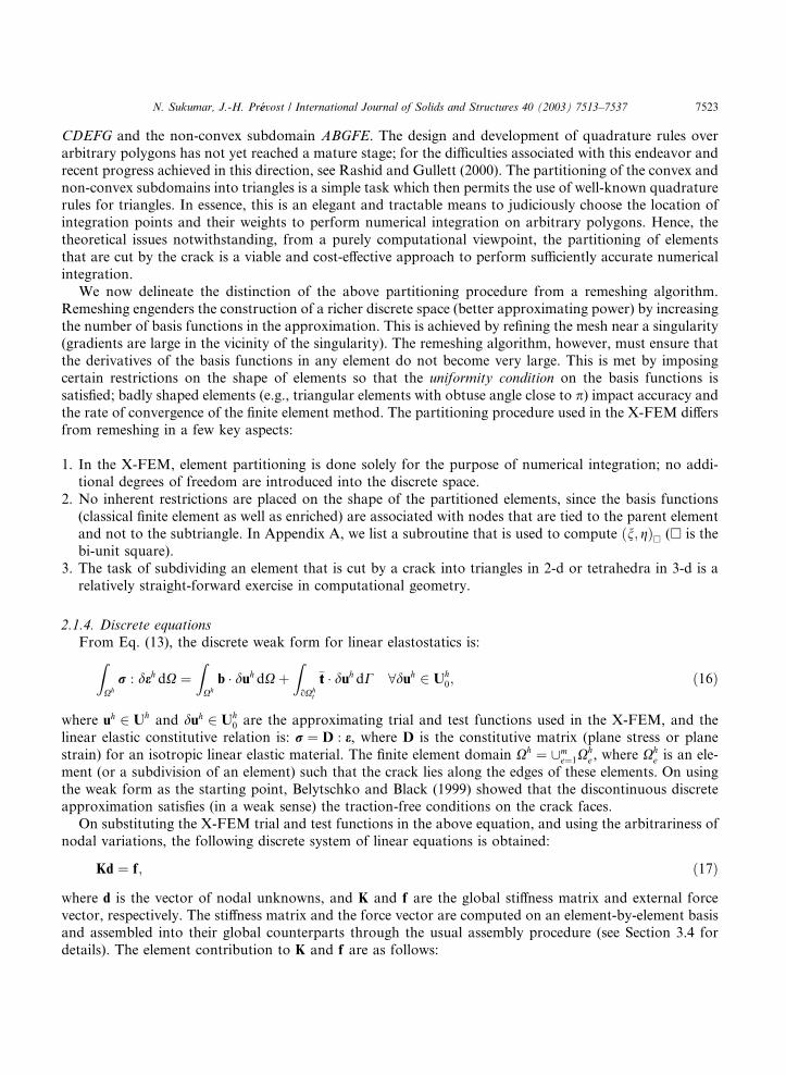
(15) is applied to each subdomain, the exact solution is recovered. On the basis of the above discussion, we

infer that the crack geometry must coincide with edges of simplexes used in the numerical integration. From

Fig. 6, we note that this can be achieved by carrying out numerical integration on the convex subdomain

Table 1

Numerical integration of discontinuous and piece-wise continuous functions

f ðxÞ No. of Gauss points ðnspÞ Q½ f I ½ f C1 1 1.5000 0.75

2 0.3750

5 0.6950

7 0.6101

10 0.7075

C0 1 0.3750 0.5

2 0.5123

5 0.5066

7 0.4996

10 0.5015


CDEFG and the non-convex subdomain ABGFE. The design and development of quadrature rules over

arbitrary polygons has not yet reached a mature stage; for the difficulties associated with this endeavor and

recent progress achieved in this direction, see Rashid and Gullett (2000). The partitioning of the convex and

non-convex subdomains into triangles is a simple task which then permits the use of well-known quadraturerules for triangles. In essence, this is an elegant and tractable means to judiciously choose the location of

integration points and their weights to perform numerical integration on arbitrary polygons. Hence, the

theoretical issues notwithstanding, from a purely computational viewpoint, the partitioning of elements

that are cut by the crack is a viable and cost-effective approach to perform sufficiently accurate numerical

integration.

We now delineate the distinction of the above partitioning procedure from a remeshing algorithm.

Remeshing engenders the construction of a richer discrete space (better approximating power) by increasing

the number of basis functions in the approximation. This is achieved by refining the mesh near a singularity(gradients are large in the vicinity of the singularity). The remeshing algorithm, however, must ensure that

the derivatives of the basis functions in any element do not become very large. This is met by imposing

certain restrictions on the shape of elements so that the uniformity condition on the basis functions is

satisfied; badly shaped elements (e.g., triangular elements with obtuse angle close to p) impact accuracy and

the rate of convergence of the finite element method. The partitioning procedure used in the X-FEM differs

from remeshing in a few key aspects:

1. In the X-FEM, element partitioning is done solely for the purpose of numerical integration; no addi-tional degrees of freedom are introduced into the discrete space.

2. No inherent restrictions are placed on the shape of the partitioned elements, since the basis functions

(classical finite element as well as enriched) are associated with nodes that are tied to the parent element

and not to the subtriangle. In Appendix A, we list a subroutine that is used to compute ðn; gÞ( is the

bi-unit square).

3. The task of subdividing an element that is cut by a crack into triangles in 2-d or tetrahedra in 3-d is a

relatively straight-forward exercise in computational geometry.

2.1.4. Discrete equations

From Eq. (13), the discrete weak form for linear elastostatics is:
ZXhr : deh dX ¼
ZXhb duh dXþ

ZoXh

t

tt duh dC 8duh 2 Uh0; ð16Þ

where uh 2 Uh and duh 2 Uh0 are the approximating trial and test functions used in the X-FEM, and the

linear elastic constitutive relation is: r ¼ D : e, where D is the constitutive matrix (plane stress or plane

strain) for an isotropic linear elastic material. The finite element domain Xh ¼ [me¼1X

he , where Xh

e is an ele-

ment (or a subdivision of an element) such that the crack lies along the edges of these elements. On using

the weak form as the starting point, Belytschko and Black (1999) showed that the discontinuous discreteapproximation satisfies (in a weak sense) the traction-free conditions on the crack faces.

On substituting the X-FEM trial and test functions in the above equation, and using the arbitrariness of

nodal variations, the following discrete system of linear equations is obtained:

Kd ¼ f; ð17Þ

where d is the vector of nodal unknowns, and K and f are the global stiffness matrix and external force

vector, respectively. The stiffness matrix and the force vector are computed on an element-by-element basisand assembled into their global counterparts through the usual assembly procedure (see Section 3.4 for

details). The element contribution to K and f are as follows:


keij ¼

kuuij kua

ij kubij

kauij kaa

ij kabij

kbuij kba

ij kbbij

264

375; ð18aÞ

fei ¼ f fui fai fb1i fb2i fb3i fb4i gT; ð18bÞ

where the submatrices and vectors that appear in Eq. (18) are defined as:

krsij ¼

ZXeðBr

i ÞTDBs

j dX ðr; s ¼ u; a; bÞ ð19aÞ

fui ¼ZoXh

t \oXeNittdCþ

ZXeNibdX; ð19bÞ

fai ¼ZoXh

t \oXeNiHttdCþ

ZXeNiHbdX; ð19cÞ

fbai ¼ZoXh

t \oXeNiUattdCþ

ZXhNiUabdX ða ¼ 1–4Þ: ð19dÞ

In the above equations, Ni is the standard finite element shape function that is defined at node i (i ¼ 1; nen)of the finite element, where nen is the number of nodes in the connectivity of the finite element. The number

of degrees of freedom ndof ¼ 2 in 2-d elasticity. Nodes in the set NC have one enriched degree of freedom

in each spatial dimension, and nodes in the set NK have four enriched degrees of freedom in each spatial

dimension––refer to Section 2.1.1. for details on the nodal sets NC and NK.In Eq. (19), Bu

i , Bai , and Bb

i are the matrix of shape function derivatives which are given by

Bui ¼

Ni;x 0

0 Ni;y

Ni;y Ni;x

24

35; ð20aÞ

Bai ¼

ðNiHÞ;x 00 ðNiHÞ;y

ðNiHÞ;y ðNiHÞ;x

24

35; ð20bÞ

Bbi ¼ ½Bb1

i Bb2i Bb3

i Bb4i ; ð20cÞ

Bbai ¼

ðNiUaÞ;x 0

0 ðNiUaÞ;yðNiUaÞ;y ðNiUaÞ;x

24

35 ða ¼ 1–4Þ: ð20dÞ

3. Computer implementation

The task of incorporating the X-FEM capabilities within a general-purpose finite element program can

be broken down into the following subcategories:

1. Input data (crack geometry, enrichment types, crack growth law)

2. Nodal degrees of freedom


3. Mesh–geometry interactions (nodal enrichment and element partitioning)

4. Assembly procedure

5. Post-processing

The central ideas and issues that are described below are based on the original development of the X-FEM

in Mo€ees et al. (1999) and Daux et al. (2000), where C++ was used as the programming language and the

tools developed within that framework were ideally-suited for the incorporation of many different appli-

cations within one code (Dolbow, 1999; Sukumar et al., 2001; Wagner et al., 2001; Sukumar et al., 2003a; Ji

et al., 2002). In the present instance, we address similar issues and describe a means to incorporate the same

capabilities within a Fortran programming environment––Dynaflowe (Preevost, 1983) is considered in

this study.

3.1. Input data

In finite elements, the finite element mesh is used to fully describe the model domain as well as theinternal boundaries (defects such as holes and cracks). In the X-FEM, the problem domain is represented

by a finite element mesh, whereas the internal boundaries such as cracks are not. The enriched displacement

approximation given in Eq. (8) is used to account for the presence of the cracks in the model. In 2-

dimensions, we represent cracks as piecewise linear segments, with the crack tip being a point in 2-space:

each crack is defined by contiguous piecewise linear segments, i.e., Cc ¼ [pi¼1li, where li ¼ fxi

a; xibg, with

xia ¼ xi1

b for i ¼ 2; 3; . . . ; p. The crack-tip(s) are either or both of x1a and x

pb.

In the input data file, the crack geometry, enrichment type for the crack, and parameters for crack

growth (evolution) are indicated. Keywords that have to appear verbatim in the data file are cast intypewriter font. A backslash (n) denotes continuation within a block, the text after an exclamation (!)

is treated as comments, and a blank line denotes the end of a block. Each model is subdivided into regions

(DEFINE_REGION) where the physical phenomenon in the region is typically described by a set of partial

differential equations. In the finite element model, a region consists of a union of finite elements and the

physics acting in the region is embedded within several ELEMENT_GROUP. This demarcation allows the

integration of multi-physics processes (thermoelastic, fluid-structure, or poroelastic) to be readily simu-

lated. Each region may consist of a link to several element groups––a crack is an element group with

geometric properties (connectivity) and a material model (properties, parameters for stress intensity factorcomputation, crack growth law, etc.). A single crack is defined within one DEFINE_ELEMENT_GROUP

block; multiple blocks are required for multiple crack definitions. Six different keywords have been defined

for crack enrichment, namely

enrichment type ¼

crack without tip ðHeavisideÞ;crack with tip 1 ðHeaviside þ crack functions at tip 1Þ;crack with tip 2 ðHeaviside þ crack functions at tip 2Þ;crack ðHeaviside þ crack fns at both tipsÞ;crack bimat tip 1 ðHeaviside þ bimat crack fns at tip 1Þ;crack bimat tip 2 ðHeaviside þ bimat crack fns at tip 2Þ;

8>>>>>>>><>>>>>>>>:

where the last two definition are for the bimaterial crack problem. A sample input file used for the extended

finite element analysis in Dynaflowe is available from the web site: http://dilbert.engr.ucdavis.edu/~suku/

xfem/dynaflow/input_dyna.dat.

http://dilbert.engr.ucdavis.edu/~suku/xfem/dynaflow/input_dyna.dat

http://dilbert.engr.ucdavis.edu/~suku/xfem/dynaflow/input_dyna.dat


3.2. Nodal degrees of freedom

In the finite element implementation for problems in 2-d linear elasticity, there are two unknowns at each

node (ndof ¼ nsd ¼ 2). These correspond to the nodal displacements in each coordinate-direction. In theextended finite element, as is evident from Eq. (8), apart from the classical degrees of freedom, additional

unknown enriched degrees of freedom are introduced via the displacement approximation. A Galerkin

procedure is used to solve for both, the classical as well as enriched degrees of freedom. Since these enriched

degrees of freedom are intrinsically based on the support properties of the shape functions associated with

the original nodes in the mesh, it is natural to associate these unknown coefficients to the nodes themselves.

In higher-order finite elements (bi-quadratic, bi-cubic, etc.), unknowns are tied to additional nodes that are

introduced along the element edges.

Arrays are assumed to start with 1 unless otherwise indicated. In Dynaflowe, the nodal integer array Id

is used to map a specific classical degree of freedom of a node to the global equation number. For the

classical finite element method, the array is: Idð1 : ndof ; 1 : nnodeÞ ¼ P , where P is the global equation

number. To accommodate the enriched degrees of freedom, a new integer array was defined for the en-

richment: IdXð1 : ndof ; 1 : ndofX ; 1 : nnodeÞ ¼ P , where the first slot is for the number of spatial degrees of

freedom. In addition, ndofX is the maximum number of enriched degrees of freedom in each coordinate

direction, and nnode is the number of nodes in the mesh. The array Id could have very easily been ex-

panded to accommodate the enrichment; however, to reduce the likelihood of any conflict with existing

applications, we chose to use a different array IdX for the enriched degrees of freedom. The value of ndofXcan be specified in the input data file within the DEFINE_PROBLEM block. If it is not specified in the data

file, the value of ndofX is inferred based on the enrichment_type indicated in the data file. For example,

if enrichment_type¼Heaviside, then ndofX ¼ 1, but if enrichment_type¼crack, then

ndofX ¼ 4 since a node cannot have both Heaviside and near-tip enrichment. In the event of multiple

cracks, this variable should be appropriately set since it is possible that more than one crack may intersect

the same element.

Now, the array IdX alone is not sufficient to fully quantify the enrichment for a crack. Since the appeal of

the X-FEM is in the treatment of multiple cracks within the same framework, one must allow for the existenceof multiple cracks within the same domain. Hence, by extension from the single crack case, when multiple

cracks are present, separate nodal enrichment is required to ensure the presence of each crack in the domain.

It follows that the enriched degrees of freedom at a node must be tied to a crack id, which would permit the

computation of the appropriate enrichment function. This suggests the need to provide an additional data

structure––a key which maps the degree of freedom information to a particular crack. This character*20

array is dimensioned as: Xdof keyð1 : ndof ; 1 : ndofX ; 1 : nnodeÞ. The name of the enrichment function is

stored in the first to the eighteenth character (name is distinct for the two crack-tips), the nineteenth character

is the enrichment function number (a ¼ 1–4 for the near-tip functions) and the twentieth character is the crackid. The Xdof key array is filled-up when the enriched nodes are selected. A simple concatenation is done

using the char function, for example Heaviside_crack_id//char(ifunc)//char(crack_id)), and the extraction is

done using the ichar function. Thus, for a direction idof (1 : ndof ) with enrichment idofX (1 : ndofX ) at

node I , the corresponding equation number is obtained as P ¼ IdXðidof ; idofX ; IÞ, and the enrichment

function number and crack number are func id ¼ icharðkeyð19 : 19ÞÞ and crack id ¼ icharðkeyð20 : 20ÞÞ,respectively, where key ¼ Xdof keyðidof ; idofX ; IÞ.

3.3. Mesh–geometry interaction

In 2-d, the finite element mesh consists of triangular and quadrilateral elements, and the crack is rep-

resented as a union of line segments with the crack-tip represented by a point. In the earlier 2-d (Daux et al.,2000) and 3-d (Sukumar et al., 2000) implementation of the X-FEM, the use of geometric predicates was


adopted. These also form an integral part in this work. In the following subsection, we discuss the concept

of geometric predicates. In carrying out the enrichment, one of the first tasks is to determine the finite

elements that intersect the crack. These finite elements are partitioned into triangles, which serves a dual

purpose––first to compute the areas of the subtriangles above and below the crack (area-criterion in Section2.1.2), and secondly so that the numerical integration of the bilinear form accounts for the discontinuities

on either side of the crack.

3.3.1. Geometric predicates

Since data is stored and computations performed using finite-precision arithmetic, it is essential that therobustness of algorithms is maintained even for small perturbations in the data. Efforts have been made to

develop robust geometric predicates (Shewchuk, 1997), which are especially important in the development

of algorithms for the Delaunay tessellation and Voronoi diagram of a point set.

The incircle and orientation tests are widely used in computational geometry. The orientation test de-

termines whether a point lies to the left of, to the right of, or on a line or plane defined by other points. The

incircle test determines whether a point lies inside, outside, or on a circle defined by other points. Each of

these tests is performed by evaluating the sign of a determinant. If the value of the determinant is close to

zero, then computing the intersection of line segments is error-prone––on using single-precision or double-precision data, round-off errors could lead to an erroneous result or even failure in the intersection algo-

rithm. Instead of explicitly computing intersections, geometric predicates provide an easier and robust

means to evaluate queries.

In the X-FEM implementation, we adopt the orientation test to determine the nodal enrichment for a

query point x and also use it in the algorithm for the partitioning of the finite elements into triangles. For a

query point x ðx; yÞ, we consider the triangle with vertices ðx1; x2; xÞ, where x1 ðx1; y1Þ and x2 ðx2; y2Þare the coordinates that define a crack segment. Twice the signed area of the triangle (determinant D) isevaluated:

D ¼ ðx1 xÞðy2 yÞ ðx2 xÞðy1 yÞ: ð21Þ

To test the orientation of a point with respect to the crack, the ternary predicates ABOVE ðD > Þ , BELOWðD < Þ, and ON ð6D6 Þ are used. A tolerance ¼ 106 is used for a finite element mesh with element

edge length of Oð1Þ.

3.3.2. Nodal enrichment and element partitioning

We first discuss the selection of the enriched nodes, then touch upon the computation of enrichment

functions, and lastly discuss the partitioning of the finite elements that are intersected by the crack. To

select the nodes for enrichment, a loop over the cracks and then over all the elements in the mesh suffices. A

bounding-box algorithm that returns all the elements (set E) in the vicinity of the crack proves to be

computationally efficient. In Fig. 8, a flowchart illustrating the selection of enriched nodes for a single crack

c is presented. The nodal enrichment information is stored in the Xdof_key array.The computation of the enrichment functions is straight-forward. For a Gauss point x in an enriched

element e, the binary predicates ABOVE (H ¼ 1) and BELOW (H ¼ 1) provide the value of H . The de-

rivative of H is zero at a Gauss point. To compute the near-tip enrichment functions, the local crack-tip

coordinate ðxloc; ylocÞ of x is determined. Using these, the polar coordinates are: r ¼ffiffiffiffiffiffiffiffiffiffiffiffiffiffiffiffiffiffiffix2loc þ y2loc

pand

h ¼ tan1ðyloc=xlocÞ. The derivatives of the near-tip enrichment functions are found in the local coordinate

system and a vector transformation is used to obtain their derivatives with respect to the global ðx; yÞCartesian coordinate system.

The element partitioning algorithm adopted in Daux et al. (2000) is described in Sukumar et al. (2000);the C++ code is also available in the public-domain (Sukumar, 2000). The C++ code was converted to

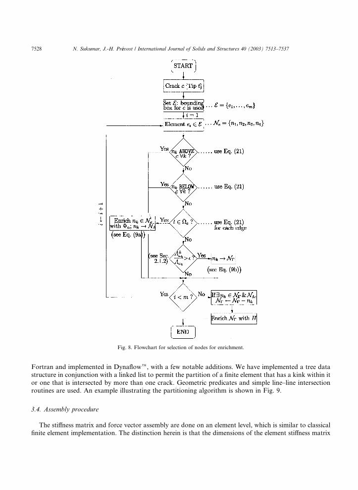
Fig. 8. Flowchart for selection of nodes for enrichment.


Fortran and implemented in Dynaflowe, with a few notable additions. We have implemented a tree data

structure in conjunction with a linked list to permit the partition of a finite element that has a kink within it

or one that is intersected by more than one crack. Geometric predicates and simple line–line intersectionroutines are used. An example illustrating the partitioning algorithm is shown in Fig. 9.

3.4. Assembly procedure

The stiffness matrix and force vector assembly are done on an element level, which is similar to classicalfinite element implementation. The distinction herein is that the dimensions of the element stiffness matrix

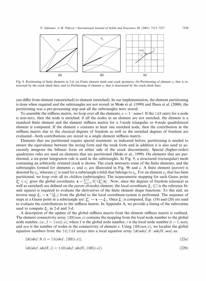
e2e1

(a) (b) (c)

e2crack

e1

Fig. 9. Partitioning of finite elements in 2-d. (a) Finite element mesh and crack geometry; (b) Partitioning of element e1 that is in-

tersected by the crack (dark line); and (c) Partitioning of element e2 that is intersected by the crack (dark line).


can differ from element (unenriched) to element (enriched). In our implementation, the element partitioning

is done when required and the subtriangles are not stored; in Mo€ees et al. (1999) and Daux et al. (2000), the

partitioning was a pre-processing step and all the subtriangles were stored.

To assemble the stiffness matrix, we loop over all the elements, e ¼ 1 : numel. If the IdX entry for a nodeis non-zero, then the node is enriched; if all the nodes in an element are not enriched, the element is a

standard finite element and the element stiffness matrix for a 3-node triangular or 4-node quadrilateral

element is computed. If the element e contains at least one enriched node, then the contribution in the

stiffness matrix due to the classical degrees of freedom as well as the enriched degrees of freedom are

evaluated––both contributions are stored in a single element stiffness matrix.

Elements that are partitioned require special treatment: as indicated before, partitioning is needed to

ensure the equivalence between the strong form and the weak form and in addition it is also used to ac-

curately integrate the bilinear form on either side of the crack discontinuity. Special (higher-order)quadrature rules are used on elements that are partitioned (Mo€ees et al., 1999). On elements that are par-

titioned, a six-point integration rule is used in the subtriangles. In Fig. 9, a structured (rectangular) mesh

containing an arbitrarily oriented crack is shown. The crack intersects some of the finite elements, and the

subtriangles formed for elements e1 and e2 are illustrated in Fig. 9b and c. A finite element (parent) is

denoted by eq, whereas eMq is used for a subtriangle (child) that belongs to eq. For an element eq that has beenpartitioned, we loop over all its children (subtriangles). The isoparametric mapping for each Gauss point

nMq 2 eMq gives the global coordinate: x ¼P3

i¼1 NM

i ðnM

q ÞxM

i . Now, since the degrees of freedom (classical as

well as enriched) are defined on the parent (4-node) element, the local coordinate n( is the reference bi-

unit square) is required to evaluate the derivatives of the finite element shape functions. To this end, an

inverse map n¼ x1ðn

Þ from the global to the local coordinate-system is performed. The sequence of

steps at a Gauss point in a subtriangle are: nMq ! x ! n. Once n

is computed, Eqs. (19) and (20) are used

to evaluate the contributions to the stiffness matrix. In Appendix A, we provide a listing of the subroutine

used to compute nin 2-d and 3-d.

A description of the update of the global stiffness matrix from the element stiffness matrix is outlined.

The element connectivity array IENðnen; eÞ contains the mapping from the local node number to the global

node number, i.e., I ¼ Ienði; eÞ, where I is the global node number, i is the local node number (i ¼ 1; nen),and nen is the number of nodes in the connectivity of element e. Using IENðnen; eÞ, we localize the global

equation numbers from the Id=IdX arrays into a local equation array LMðndof ; 0 : ndofX ; nenÞ as:

LMðidof ; 0; iÞ ¼ Idðidof ;IENði; eÞÞ; ð22aÞ

LMðidof ; idofX ; iÞ ¼ IdXðidof ; idofX ;IENði; eÞÞ: ð22bÞ


The element stiffness matrix and element force vector are assembled into local arrays ke and fe with

dimensions keðnee; neeÞ and feðneeÞ, respectively, where the dimension nee ¼ ndof ð1þ ndofX Þnen. Theassembly of the local stiffness matrix and the external force vector for element e proceeds in a straight-

forward and classical fashion in which ke and fe are passed to assembly routines where looping over thelocal equation numbers is carried out:

do p ¼ 1, nee

P ¼ LMðpÞif (P > 0) then

do q ¼ 1, nee

Q ¼ LMðqÞif ðQ > 0Þ then

KðP ;QÞ ¼ KðP ;QÞ þ keðp; qÞendif

enddo

f ðP Þ ¼ f ðPÞ þ feðpÞendif

end

3.5. Post-processing

In the X-FEM, the degrees of freedom in unenriched elements are synonymous with nodal displace-

ments. However, the classical degrees of freedom in an enriched element are in general no longer the nodal

displacement––the nodal displacement is found by evaluating Eq. (8) at an enriched node. Since dis-

placement plots are required to check the presence of the discontinuity and also to plot the deformed shape,

it is desirable to expedite the evaluation of the displacement at the nodes. To this end, the values of the

enrichment functions at the nodes are stored in an array. Since HðxÞ is undefined at a node (say nI ) that lieson the crack, the enrichment function is multi-valued (+1 and )1). This also applies to the first near-tip

function in Eq. (2), namelyffiffir

psinðh=2Þ, which is discontinuous across the crack (h ¼ p). Since nodal

output is element-based, in both cases, the appropriate sign is selected by knowing the element e under

consideration (nI 2 Ne). A simple check using the geometric predicates at xc (center of element e) provides(ABOVE or BELOW) the sign to be used.

Fracture parameters such as the mode I and mode II stress intensity factors (SIFs) are determined using

the domain form (Li et al., 1985; Moran and Shih, 1987) of the interaction integral (Yau et al., 1980). In the

X-FEM, due to the enrichment with the near-tip fields, the SIFs can be expressed as a linear combination ofthe enriched coefficients. If the crack-tip Kc is inside an element e, then for a pure mode I problem in 2-d,

the expression for KI is:

KI ¼Effiffiffiffiffiffi2p

p

4ð1 m2ÞXneni¼1

NiðxÞb12i; x 2 Kc; ð23Þ

where Ni is the finite element shape function for node i, and b12i are enriched coefficients that are tied to the

near-tip function U1 and to the displacement approximation in x2-direction. However, extraction of the

SIFs directly from these coefficients is not sufficiently accurate. In general, the use of crack-tip flux integrals

leads to better accuracy than even extrapolation (displacement or stress) techniques. In the domain integral

form of the interaction integral, the numerical computations are carried out in elements (by appropriate

choice of the weighting function) that are distant from the crack-tip; in these elements the field quantitiesare much more accurate than those in the vicinity of the crack-tip. For SIF computations, the domain form


of path-independent flux integrals is also used in commercial finite element codes (e.g., ABAQUSe); we

adopt the same approach for the computation of stress intensity factors in this implementation. The

J -integral is related to the mixed mode SIFs through the relation:

J ¼ K2I

E þK2

II

E ; E ¼E ðplane stressÞ;E

1 m2ðplane strainÞ;

(ð24Þ

where E and m are the Youngs modulus and Poissons ratio, respectively.In the interaction integral method (Yau et al., 1980), the 2-d plane strain auxiliary fields are introduced

and superposed on the actual fields that arise from the solution of the boundary-value problem. By judi-

cious choice of the auxiliary fields, the interaction integral can be directly related to the mixed-mode stress

intensity factors. The domain form of the interaction integral is computed on these elements (Yau et al.,

1980). The domain form of the interaction integral is a well-established technique to determine mixed-mode

SIFs in fracture computations with the finite element method. All the finite elements within a radius of

rd ¼ rkhe from the crack-tip are selected. Here, he is the crack-tip element size and rk is a scalar multiple. Allelements within a radius of rd from the crack-tip are marked. Let us denote this element set by Nd

e , with Xhd

defining the resulting discrete (union of elements) domain. The weighting function q that appears in the

domain form of the interaction integral is then set: if a node ni that is contained in the connectivity of

element e 2 Nde lies on the boundary oXh

d , then qi ¼ 0; if node ni lies in Xhd , then qi ¼ 1. Since the gradient of

q appears in the domain integral expression, non-zero contribution to the integral in the numerical com-

putations is obtained only for elements with an edge that lies on oXhd . For additional details on the eva-

luation of the SIFs in the X-FEM, see Mo€ees et al. (1999).Some of the well-known crack growth criteria are: maximum hoop (circumferential) stress criterion

(Erdogan and Sih, 1963); maximum energy release rate criterion (Nuismer, 1975); and the maximum strain

energy density criterion (Sih, 1974). These criteria predict slightly different angles for the initial kink, but

they all predict that once the kink is initiated, the crack trajectory is such that KII ¼ 0 (principle of local

symmetry). The maximum hoop stress criterion (Erdogan and Sih, 1963) gives the crack growth direction:

hc ¼ 2 tan1 1

4

KI

KII

0@

ffiffiffiffiffiffiffiffiffiffiffiffiffiffiffiffiffiffiffiffiffiffiffiffiffiKI

KII

2

þ 8

s 1A; ð25Þ

where hc is the crack growth angle in the local crack-tip coordinate system. If KII ¼ 0 then hc ¼ 0 (pure

mode I). By noting that if KII > 0, the crack growth angle hc < 0, and if KII < 0, then hc > 0, a compu-

tationally more amenable expression for hc is implemented (Suo, 2002):

hc ¼ 2 tan1 2KII=KI

1þffiffiffiffiffiffiffiffiffiffiffiffiffiffiffiffiffiffiffiffiffiffiffiffiffiffiffiffiffiffi1þ 8 KII=KIð Þ2

q264

375; ð26Þ

where w ¼ tan1ðKII=KIÞ, the mode angle, is a measure of the ratio of mode II to mode I . The application of

the X-FEM to crack growth problems is presented in Part II (Huang et al., 2003b), which follows this

publication.

4. Conclusions

In this paper (Part I of a two-part series), we have demonstrated a simple and robust means to im-

plement the modeling of discontinuous fields within an existing finite element program. The methodologyadopted for modeling crack discontinuities falls within the purview of the extended finite element method


(X-FEM) (Mo€ees et al., 1999; Daux et al., 2000), which is a particular instance of the partition of unity

method (Melenk and Babusska, 1996; Duarte and Oden, 1996). The finite element program Dynaflowe

(Preevost, 1983) was used in this study, and the implementation for crack modeling in isotropic and bi-

material media was described. Issues pertaining to the selection of nodes for enrichment, computation ofthe enrichment functions, array-allocation for the enriched nodal degrees of freedom, mesh–geometry in-

teractions, and assembly of the global stiffness matrix and external force vector were addressed. This study

has provided the capability and revealed the relative ease by which discontinuous fields through the par-

tition of unity framework can be incorporated within a standard finite element package.

Acknowledgements

The financial support to J.-H.P. from the National Science Foundation through contract NSF-9988788,

Dr. Jorn Larsen-Basse Program Manager, is gratefully acknowledged. This work was accomplished in

Spring 2001 when N.S. was visiting Princeton University; the hospitality extended to him by Professor

David Srolovitz is appreciated. The comments and suggestions of the anonymous reviewers are also ac-

knowledged.

Appendix A

Assume that a quadrilateral element which is cut by a crack is partitioned into triangular elements. The

bilinear form (stiffness matrix) is computer over each subtriangle. On knowing the physical coordinates

ðx; yÞ of a point within a subtriangle, the local coordinates ðn; gÞ( is the bi-unit square that is mapped to

the quadrilateral) are required to compute the finite element shape functions and their derivatives. The

Fortran code to carry out the transformation follows; a Newton–Raphson iterative algorithm is used.

c***********************************************************************

subroutine inversemap(xy,x,xe,nsd,nen,topo)

c Purpose:Compute the inverse mapping from the physical space to

c ¼ ¼ ¼ ¼ the reference element for 2-d and 3-d finite elements

c

c Input

c ¼ ¼ ¼c nodal coordinates :xy(nsd,nen)

c coordinates :x(nsd) in physical space

c topo :character array (topology of the element)

c nsd¼number of space dimensions, nen¼number of nodes/element

c Output

c ¼ ¼ ¼c local coordinates:xe(1)¼xi, xe(2)¼eta, xe(3)¼zeta in the

c reference bi-unit square/cube

c***********************************************************************

c

implicit real*8 (a-h,o-z)

parameter (Nsd_max¼3, Nen_max¼8)

c

character*(*) topo

dimension xy(nsd,*), x(*), xe(*)


dimension xs(Nsd_max*Nsd_max), sh((Nsd_max+1)*Nen_max)

dimension point(Nsd_max), xe_new(Nsd_max)

parameter (iter_max¼50, err_tol¼1.d-8)

nshp¼nsd+1

c

c initialize

iter¼0

call dclear(xe,nsd) !clear the array

1 iter¼iter+1

c

c get shape functions at xe

call shapl(xe,sh,nen,nshp,nsd,0,topo)

c

c compute inverse of the jacobian map

call xjacobian(xs,xy,nsd,sh,nshp,nen)

c

c compute coordinates of point

call dclear(point,nsd)

do i¼1,nsd

do j¼1,nen

point(i)¼point(i)+sh((nsd+1)+nshp*(j)1))*xy(i,j)

enddo

enddo

c

c update xe

do i¼1,nsd

xe_new(i)¼xe(i)

do j¼1,nsd

xe_new(i)¼xe_new(i)+xs(i+nsd*(j)1))*(x(j))point(j))

enddo

enddo

c

c error

do i¼1,nsd

xe(i)¼xe_new(i))xe(i)

enddo

err¼sqrt(dotl(xe,xe,nsd)) !dotl (function for dot product)

calldmove(xe,xe_new,nsd) !move xe_new to xe

if (err .le.err_tol) then

goto 99

elseif (iter .lt.iter_max) then

goto 1

else

call pend(0inversemap:convergence failed0) !error message

endif

99 return

end

c***********************************************************************


subroutine xjacobian(xs,xl,nsd,sh,nshp,nen)

c Purpose:Compute the inverse of the jacobian map

c Output

c ¼ ¼ ¼c xs(nsd,nsd) :inverse of the jacobian map

c***********************************************************************

c

implicit real*8 (a-h,o-z)

dimension xs(nsd,*), xl(nsd,*), sh(Nshp,*)

dimension cof(3,3), xinv(3,3)

parameter (zero¼0.d0, one¼1.d0)

call dclear(xs,nsd*nsd)

do i¼1,nsd

do j¼1,nsd

do k¼1,nen

xs(i,j)¼xs(i,j)+xl(i,k)*sh(j,k)

enddo

enddo

enddo

if (nsd .eq.2) then

det¼xs(1,1)*xs(2,2))xs(1,2)*xs(2,1)

if (det .le.zero) call pend(0xjacobian:det .le.00)call dotacl(xs,one/det,nsd*nsd)

tmp¼xs(1,1)

xs(1,1)¼xs(2,2)

xs(2,2)¼tmp

xs(1,2)¼)xs(1,2)xs(2,1)¼)xs(2,1)

else

COF(1,1)¼XS(2,2)*XS(3,3))XS(3,2)*XS(2,3)

COF(1,2)¼XS(2,3)*XS(3,1))XS(2,1)*XS(3,3)

COF(1,3)¼XS(2,1)*XS(3,2))XS(3,1)*XS(2,2)

COF(2,1)¼XS(3,2)*XS(1,3))XS(1,2)*XS(3,3)

COF(2,2)¼XS(1,1)*XS(3,3))XS(3,1)*XS(1,3)

COF(2,3)¼XS(3,1)*XS(1,2))XS(1,1)*XS(3,2)

COF(3,1)¼XS(1,2)*XS(2,3))XS(2,2)*XS(1,3)

COF(3,2)¼XS(2,1)*XS(1,3))XS(1,1)*XS(2,3)

COF(3,3)¼XS(1,1)*XS(2,2))XS(2,1)*XS(1,2)

det¼XS(1,1)*COF(1,1)+XS(1,2)*COF(1,2)+XS(1,3)*COF(1,3)

if (det .le.zero) call pend(0xjacobian:det .le.00)

call dotacl(xs,one/det,nsd*nsd)

XINV(1,1)¼ (XS(2,2)*XS(3,3))XS(3,2)*XS(2,3))

XINV(1,2)¼)(XS(1,2)*XS(3,3))XS(3,2)*XS(1,3))

XINV(1,3)¼ (XS(1,2)*XS(2,3))XS(2,2)*XS(1,3))

XINV(2,1)¼)(XS(2,1)*XS(3,3))XS(3,1)*XS(2,3))

XINV(2,2)¼ (XS(1,1)*XS(3,3))XS(3,1)*XS(1,3))


XINV(2,3)¼)(XS(1,1)*XS(2,3))XS(2,1)*XS(1,3))

XINV(3,1)¼ (XS(2,1)*XS(3,2))XS(3,1)*XS(2,2))

XINV(3,2)¼)(XS(1,1)*XS(3,2))XS(3,1)*XS(1,2))

XINV(3,3)¼ (XS(1,1)*XS(2,2))XS(2,1)*XS(1,2))

call dmove(xs,xinv,nsd*nsd)

endif

c

return

end

References

Armero, F., Garikipati, K., 1996. An analysis of strong discontinuities in multiplicative finite strain plasticity and their relation with

the numerical simulation of strain localization in solids. International Journal of Solids and Structures 33, 2863–2885.

Ayhan, A.O., Nied, H.F., 2002. Stress intensity factors for three-dimensional surface cracks using enriched finite elements.

International Journal for Numerical Methods in Engineering 54 (6), 899–921.

Belytschko, T., Black, T., 1999. Elastic crack growth in finite elements with minimal remeshing. International Journal for Numerical

Methods in Engineering 45 (5), 601–620.

Belytschko, T., Fish, J., Engelmann, B.E., 1988. A finite element with embedded localization zones. Computer Methods in Applied

Mechanics and Engineering 70, 59–89.

Belytschko, T., Lu, Y.Y., Gu, L., 1994. Element-free Galerkin methods. International Journal for Numerical Methods in Engineering

37, 229–256.

Belytschko, T., Mo€ees, N., Usui, S., Parimi, C., 2001. Arbitrary discontinuities in finite elements. International Journal for Numerical


Benzley, S.E., 1974. Representation of singularities with isoparametric finite elements. International Journal for Numerical Methods in

Engineering 8, 537–545.

Beuth, J.L., 1992. Cracking of thin bonded films in residual tension. International Journal of Solids and Structures 29, 1657–1675.

Bogy, D.B., 1971. On the plane elastostatic problem of a loaded crack terminating at a material interface. Journal of Applied

Mechanics 38, 911–918.

Bolzon, G., Corigliano, A., 2000. Finite elements with embedded displacement discontinuity: a generalized variable formulation.


Borja, R., 2000. A finite element model for strain localization analysis of strongly discontinuous fields based on standard Galerkin

approximation. Computer Methods in Applied Mechanics and Engineering 190, 1529–1549.

Camacho, G.T., Ortiz, M., 1996. Computational modeling of impact damage in brittle materials. International Journal of Solids and

Structures 33, 2899–2938.

Chen, D.H., 1994. A crack normal to and terminating at a bimaterial interface. Engineering Fracture Mechanics 49 (4), 517–532.

Chessa, J., Smolinski, P., Belytschko, T., 2002. The extended finite element method (XFEM) for solidification problems. International

Journal for Numerical Methods in Engineering 53 (8), 1959–1977.

Chopp, D.L., Sukumar, N., 2003. Fatigue crack propagation of multiple coplanar cracks with the coupled extended finite element

method/fast marching method. International Journal of Engineering Science 41 (8), 845–869.

Cook, T.S., Erdogan, F., 1972. Stresses in bonded materials with a crack perpendicular to the crack. International Journal of

Engineering Science 10, 677–697.

Daux, C., Mo€ees, N., Dolbow, J., Sukumar, N., Belytschko, T., 2000. Arbitrary cracks and holes with the extended finite element

method. International Journal for Numerical Methods in Engineering 48 (12), 1741–1760.

Dolbow, J., 1999. An Extended Finite Element Method with Discontinuous Enrichment for Applied Mechanics. Ph.D. thesis,

Theoretical and Applied Mechanics, Northwestern University, Evanston, IL, USA.

Dolbow, J., Nadeau, J., 2002. On the use of effective properties for the fracture analysis of microstructured materials. Engineering

Fracture Mechanics 69 (14–16), 1607–1634.

Dolbow, J., Mo€ees, N., Belytschko, T., 2000a. Discontinuous enrichment in finite elements with a partition of unity method. Finite

Elements in Analysis and Design 36, 235–260.

Dolbow, J., Mo€ees, N., Belytschko, T., 2000b. Modeling fracture in Mindlin–Reissner plates with the extended finite element method.

International Journal of Solids and Structures 57 (48–50), 7161–7183.

Dolbow, J., Mo€ees, N., Belytschko, T., 2001. An extended finite element method for modeling crack growth with frictional contact.

Computer Methods in Applied Mechanics and Engineering 190 (51–52), 6825–6846.


Duarte, C.A., Oden, J.T., 1996. An H-p adaptive method using clouds. Computer Methods in Applied Mechanics and Engineering

139, 237–262.

Duarte, C.A., Babusska, I., Oden, J.T., 1998. October generalized finite element methods for three dimensional structural mechanics

problems. In: Atluri, S.N., ODonoghue, P.E. (Eds.), Modeling and Simulation Based Engineering: Proceedings of the

International Conference on Computational Engineering Science, vol. I, Atlanta, GA. Tech. Science Press, pp. 53–58.

Duarte, C.A., Hamzeh, O.N., Liszka, T.J., Tworzydlo, W.W., 2001. The element partition method for the simulation of three-

dimensional dynamic crack propagation. Computer Methods in Applied Mechanics and Engineering 119 (15–17), 2227–2262.

Dundurs, J., 1969. Edge-bonded dissimilar orthogonal elastic wedges. Journal of Applied Mechanics 36, 650–652.

Dvorkin, E.N., Cuiti~nno, A.M., Gioia, G., 1990. Finite elements with displacement interpolated embedded localization lines insensitive

to mesh size and distortions. International Journal for Numerical Methods in Engineering 30, 541–564.

Erdogan, F., Sih, G.C., 1963. On the crack extension in plates under plane loading and transverse shear. Journal of Basic Engineering

85, 519–527.

Fleming, M., Chu, Y.A., Moran, B., Belytschko, T., 1997. Enriched element-free Galerkin methods for crack tip fields. International

Journal for Numerical Methods in Engineering 40, 1483–1504.

Gifford Jr., L.N., Hilton, P.D., 1978. Stress intensity factors by enriched finite elements. Engineering Fracture Mechanics 10, 485–496.

Gravouil, A., Mo€ees, N., Belytschko, T., 2002. Non-planar 3D crack growth by the extended finite element and the level sets––Part II:

level set update. International Journal for Numerical Methods in Engineering 53 (11), 2569–2586.

Huang, R., Preevost, J.H., Huang, Z.Y., Suo, Z., 2003a. Channel-cracking of thin films with the extended finite element method.

Engineering Fracture Mechanics 70 (18), 2513–2526.

Huang, R., Sukumar, N., Preevost, J.-H., 2003b. Modeling quasi-static crack growth with the extended finite element method. Part II:

numerical applications. International Journal of Solids and Structures, in this issue.

Hughes, T.J.R., 1987. The Finite Element Method. Prentice-Hall, Englewood Cliffs, NJ.

Ji, H., Chopp, D., Dolbow, J.E., 2002. A hybrid extended finite element/level set method for modeling phase transformations.


Jiraasek, M., 2000. Comparative study on finite elements with embedded discontinuities. Computer Methods in Applied Mechanics and

Engineering 188, 307–330.

Larsson, R., Runesson, K., 1996. Element-embedded localization band based on regularized displacement discontinuity. ASCE

Journal of Engineering Mechanics 12, 402–411.

Larsson, R., Steinmann, P., Runesson, K., 1999. Finite element embedded localization band for finite strain plasticity based on a

regularized strong discontinuity. Mechanics of Cohesive-Frictional Materials 4 (2), 171–194.

Li, F.Z., Shih, C.F., Needleman, A., 1985. A comparison of methods for calculating energy release rates. Engineering Fracture

Mechanics 21 (2), 405–421.

Lotfi, H.R., Sheng, P.B., 1995. Embedded representations of fracture in concrete with mixed finite elements. International Journal for

Numerical Methods in Engineering 38, 1307–1325.

Melenk, J.M., Babusska, I., 1996. The partition of unity finite element method: basic theory and applications. Computer Methods in

Applied Mechanics and Engineering 139, 289–314.

Merle, R., Dolbow, J., 2002. Solving thermal and phase change problems with the extended finite element method. Computational

Mechanics 28 (5), 339–350.

Mo€ees, N., Belytschko, T., 2002. Extended finite element method for cohesive crack growth. Engineering Fracture Mechanics 69 (7),

813–833.

Mo€ees, N., Dolbow, J., Belytschko, T., 1999. A finite element method for crack growth without remeshing. International Journal for

Numerical Methods in Engineering 46 (1), 131–150.

Mo€ees, N., Gravouil, A., Belytschko, T., 2002. Non-planar 3D crack growth by the extended finite element and level sets. Part I:

mechanical model. International Journal for Numerical Methods in Engineering 53 (11), 2549–2568.

Moran, B., Shih, C.F., 1987. Crack tip and associated domain integrals from momentum and energy balance. Engineering Fracture

Mechanics 27 (6), 615–641.

Nuismer, R., 1975. An energy release rate criterion for mixed mode fracture. International Journal of Fracture 11, 245–250.

Oden, J.T., Duarte, C.A., Zienkiewicz, O.C., 1998. A new cloud-based hp finite element method. Computer Methods in Applied

Mechanics and Engineering 153 (1–2), 117–126.

Ortiz, M., Leroy, Y., Needleman, A., 1987. A finite element method for localized failure analysis. Computer Methods in Applied

Mechanics and Engineering 61, 189–214.

Preevost, J.-H., 1983. Dynaflow. Princeton University, Princeton, NJ 08544 (updated version: 2002).

Rashid, M.M., Gullett, P.M., 2000. On a finite element method with variable element topology. Computer Methods in Applied

Mechanics and Engineering 190 (11–12), 1509–1527.

Regueiro, R.A., Borja, R.I., 2001. Plane strain finite element analysis of pressure sensitive plasticity with strong discontinuity.

International Journal of Solids and Structures 38 (21), 3647–3672.


Shewchuk, J.R., 1997. Adaptive precision floating-point arithmetic and fast robust geometric predicates. Discrete and Computational

Geometry 18, 305–363.

Sih, G.C., 1974. Strain energy density factor applied to mixed mode crack problems. International Journal of Fracture 10, 305–321.

Simo, J.C., Oliver, J., 1994. Modelling strong discontinuities in solid mechanics by means of strain softening constitutive equations. In:

Mang, H., Biccanicc, N., de Borst, R. (Eds.), Computational Modelling of Concrete Structures. Pineridge, Swansea, pp. 363–372.

Simo, J.C., Oliver, J., Armero, F., 1993. An analysis of strong discontinuities induced by strain softening in rate-independent inelastis

solids. Computational Mechanics 12, 277–296.

Sluys, L.J., Berends, A.H., 1998. Discontinuous failure analysis for mode-I and mode-II localization problems. International Journal

of Solids and Structures 35, 4257–4274.

Stolarska, M., Chopp, D.L., Mo€ees, N., Belytschko, T., 2001. Modeling crack growth by level sets and the extended finite element

method. International Journal for Numerical Methods in Engineering 51 (8), 943–960.

Strouboulis, T., Babusska, I., Copps, K., 2000. The design and analysis of the generalized finite element method. Computer Methods in

Applied Mechanics and Engineering 181 (1–3), 43–69.

Strouboulis, T., Copps, K., Babusska, I., 2001. The generalized finite element method. Computer Methods in Applied Mechanics and

Engineering 190 (32–33), 4081–4193.

Sukumar, N., 2000. Element partitioning code in 2-d and 3-d for the extended finite element method. Available from <http://

dilbert.engr.ucdavis.edu/~suku/xfem.

Sukumar, N., Mo€ees, N., Moran, B., Belytschko, T., 2000. Extended finite element method for three-dimensional crack modeling.


Sukumar, N., Chopp, D.L., Mo€ees, N., Belytschko, T., 2001. Modeling holes and inclusions by level sets in the extended finite-element

method. Computer Methods in Applied Mechanics and Engineering 190 (46–47), 6183–6200.

Sukumar, N., Chopp, D.L., Moran, B., 2003a. Extended finite element method and fast marching method for three dimensional fatigue

crack propagation. Engineering Fracture Mechanics 70 (1), 29–48.

Sukumar, N., Srolovitz, D.J., Baker, T.J., Preevost, J.-H., 2003b. Brittle fracture in polycrystalline microstructures with the extended

finite element method. International Journal for Numerical Methods in Engineering 56 (14), 2015–2037.

Sukumar, N., Huang, Z.Y., Preevost, J.-H., Suo, Z., in press. Partition of unity enrichment for bimaterial interface cracks. International

Journal for Numerical Methods in Engineering.

Suo, Z., 2002. Private communication.

Wagner, G., Mo€ees, N., Liu, W.K., Belytschko, T., 2001. The extended finite element method for rigid particles in Stokes flow.


Wells, G.N., Sluys, L.J., 2001. A new method for modelling cohesive cracks using finite elements. International Journal for Numerical


Wells, G.N., Sluys, L.J., deBorst, R., 2002. A p-adaptive scheme for overcoming volumetric locking during plastic flow. Computer

Methods in Applied Mechanics and Engineering 191 (29–30), 3153–3164.

Xu, X.-P., Needleman, A., 1994. Numerical simulations of fast crack growth in brittle solids. Journal of the Mechanics and Physics of

Solids 42, 1397–1434.

Yau, J.F., Wang, S.S., Corten, H.T., 1980. A mixed-mode crack analysis of isotropic solids using conservation laws of elasticity.

Journal of Applied Mechanics 47, 335–341.

Zak, A.R., Williams, M.L., 1963. Crack point singularities at a bimaterial interface. Journal of Applied Mechanics 30, 142–143.

http://dilbert.engr.ucdavis.edu/~suku/xfem

http://dilbert.engr.ucdavis.edu/~suku/xfem

Documents

Modeling quasi-static crack growth with the extended ﬁnite element ...dilbert.engr.ucdavis.edu/~suku/xfem/papers/xfem_partI.pdf · and the crack path are outcomes of the analysis