Embed Size (px)
Citation preview
Parametric Sensitivities of XFEM Based Prognosis for
Quasi-static Tensile Crack Growth
Siddharth Prasanna Kumar
Thesis submitted to the faculty of the Virginia Polytechnic Institute and State University in
partial fulfillment of the requirements for the degree of
Master of Science
In
Mechanical Engineering
Javid Bayandor, Chair
Reza Mirzaeifar
Robert West
July 17th, 2017
Blacksburg, Virginia
Keywords: XFEM, Crack propagation, Abaqus, parametric study
Parametric Sensitivities of XFEM Based Prognosis for
Quasi-static Tensile Crack Growth
Siddharth Prasanna Kumar
Abstract
Understanding failure mechanics of mechanical equipment is one of the most important aspects of
structural and aerospace engineering. Crack growth being one of the major forms of failure in
structural components has been studied for several decades to achieve greater reliability and
guarantee higher safety standards.
Conventional approaches using the finite element framework provides accurate solutions, yet they
require extremely complicated numerical approaches or highly fine mesh densities which is
computationally expensive and yet suffers from several numerical instabilities such as element
entanglement or overly soften element behavior. The eXtended Finite Element Method (XFEM)
is a relatively recent concept developed for modeling geometric discontinuities and singularities
by introducing the addition of new terms to the classical shape functions in order to allow the finite
element formulation to remain the same. XFEM does not require the necessity of computationally
expensive numerical schemes such as active remeshing and allows for easier crack representation.
In this work, verifies the validity of this new concept for quasi-static crack growth in tension with
Abaqus’ XFEM is employed. In the course of the work, the effect of various parameters that are
involved in the modelling of the crack are parametrically analyzed.
The load-displacement data and crack growth were used as the comparison criterion. It was found
that XFEM is unable to accurately represent crack growth in the models in the elastic region
without direct manipulation of the material properties. The crack growth in the plastic region is
found to be affected by certain parameters allowing us to tailor the model to a small degree. This
thesis attempts to provide a greater understanding into the parametric dependencies of XFEM
crack growth.

Parametric Sensitivities of XFEM Based Prognosis for
Quasi-static Tensile Crack Growth
Siddharth Prasanna Kumar
General Audience Abstract
Crack propagation is one of the major causes of failure in equipment in structural and aerospace
engineering. The study of fracture and crack growth has been taking place for decades in an effort
to increase quality of design and to ensure higher standards of safety.
In the past, an accurate representation of crack growth within a specimen using conventional
numerical analysis was computationally expensive. The eXtended Finite Element Method
(XFEM) is a concept introduced that would reduce computational effort yet improving the fidelity
of the analysis while allowing for easier representation of crack growth.
This thesis, verifies the validity of XFEM in simulating crack growth in a specimen undergoing
tension using a commercially available code, Abaqus. The various parameters involved in the
modeling of this crack and their effects are studied. The study had shown that the inaccuracy of
XFEM in its ability to model crack growth, however, it gives us some understanding into certain
parameters that would allow us to tailor the model to better represent experimental data.
.
iv
Table of Contents 1. Introduction ........................................................................................................................................... 1
1.1. Context .......................................................................................................................................... 1
1.2. Objective ....................................................................................................................................... 2
2. Theory ................................................................................................................................................... 4
2.1. Theory of Linear Elastic Fracture Mechanics ............................................................................... 4
2.1.1. Griffith’s Criterion ................................................................................................................ 4
2.1.2. Modifications to Griffith’s Theory ....................................................................................... 6
2.1.3. Stress Distribution Around the Crack ................................................................................... 8
2.1.4. Loading Modes ..................................................................................................................... 9
2.1.5. Stress Intensity Factor ......................................................................................................... 10
2.1.6. Strain Energy Release Rate ................................................................................................. 13
2.1.7. Fracture Toughness testing ................................................................................................. 14
2.2. Theory of Elastic Plastic Fracture Mechanics ............................................................................. 16
2.2.1. Plastic Zone Adjustment ..................................................................................................... 16
2.2.2. Crack Tip Opening Displacement (CTOD) ........................................................................ 17
2.2.3. R-Curve ............................................................................................................................... 19
2.2.4. J-Integral ............................................................................................................................. 20
2.3. The Finite Element Method (FEM) ............................................................................................ 23
2.3.1. Methodology of FEM.......................................................................................................... 23
2.3.2. Formulation of Finite Element Equations ........................................................................... 24
2.3.3. FEM in Solid Mechanics ..................................................................................................... 28
2.3.4. Element Types..................................................................................................................... 31
2.4. Extended finite element method ................................................................................................. 31
2.4.1. XFEM enrichment- Jump Function .................................................................................... 32
2.4.2. XFEM Enrichment: Asymptotic Near-Tip Singularity Functions ...................................... 34
3. Experiment Description ...................................................................................................................... 35
3.1. Xia et al. models ......................................................................................................................... 35
3.1.1. Single Edge Notch Test (SENT) ......................................................................................... 35
3.1.2. Double Edged Notch Test (DENT) ..................................................................................... 36
3.1.3. Compact Tension Test (CT) ................................................................................................ 37
3.2. Compact Tension Test (CT) from Dowling et al. ....................................................................... 39
4. Modeling Approach ............................................................................................................................ 41
v
4.1. Part module ................................................................................................................................. 41
4.2. Property module .......................................................................................................................... 41
4.3. Assembly module and Step module ............................................................................................ 43
4.4. Interaction module ...................................................................................................................... 43
4.5. Load module ............................................................................................................................... 44
4.6. Mesh module and Job module .................................................................................................... 45
5. Parametric Analysis ............................................................................................................................ 47
5.1. Single Edge Notch Test SENT .................................................................................................... 47
5.1.1. Pin-less Loading (Fully Coupled) ....................................................................................... 47
5.1.2. Pin-less Loading (Semi Coupled) ....................................................................................... 61
5.1.3. Rigid Pin Loading ............................................................................................................... 69
5.1.4. Deformable Pin Loading ..................................................................................................... 76
5.1.5. Plastic Zone Comparison .................................................................................................... 83
5.1.6. Fracture-Plasticity Study ..................................................................................................... 84
5.1.7. Partition Study .................................................................................................................... 93
5.1.8. Element Type .................................................................................................................... 117
5.1.9. Tolerance ........................................................................................................................... 121
5.1.10. Damage Stability Cohesive ............................................................................................... 125
5.1.11. Stress Intensity Factor ....................................................................................................... 129
5.2. Double Edged Notch Test DENT ............................................................................................. 131
5.2.1. Rigid Pin Loading with Unstructured Mesh ..................................................................... 131
5.2.2. Partition Study .................................................................................................................. 136
5.2.3. Fracture-Plasticity study ................................................................................................... 147
5.2.4. Tolerance ........................................................................................................................... 149
5.2.5. Damage Stability Cohesive ............................................................................................... 152
5.2.6. Stress Intensity Factor ....................................................................................................... 154
5.3. Compact Tension Test CT ........................................................................................................ 156
5.3.1. Rigid Pin Loading with Unstructured Mesh ..................................................................... 156
5.3.2. Partition Study .................................................................................................................. 161
5.3.3. Fracture-Plasticity Study ................................................................................................... 172
5.3.4. Tolerance ........................................................................................................................... 175
5.3.5. Damage Stability Cohesive ............................................................................................... 179
5.3.6. Stress Intensity Factor ....................................................................................................... 182
vi
5.4. Compact Tension Test (CT) from Dowling et al. ..................................................................... 184
5.4.1. Mesh study ........................................................................................................................ 185
5.4.2. Non-linear Geometry ........................................................................................................ 186
5.4.3. Damage Stability Cohesive ............................................................................................... 188
5.4.4. Final Simulation ................................................................................................................ 190
5.5. Contour Plot Study .................................................................................................................... 192
6. Summary and Conclusion ................................................................................................................. 197
7. Contributions and Future work ......................................................................................................... 199
References ................................................................................................................................................. 201
Appendix A ............................................................................................................................................... 204
Damage stability cohesive – Tolerance – Mesh testing ........................................................................ 204
Solver testing ........................................................................................................................................ 206
Non-linear Geometry ............................................................................................................................ 207
vii
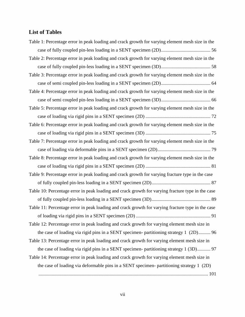
List of Tables
Table 1: Percentage error in peak loading and crack growth for varying element mesh size in the
case of fully coupled pin-less loading in a SENT specimen (2D) ......................................... 56
Table 2: Percentage error in peak loading and crack growth for varying element mesh size in the
case of fully coupled pin-less loading in a SENT specimen (3D) ......................................... 58
Table 3: Percentage error in peak loading and crack growth for varying element mesh size in the
case of semi coupled pin-less loading in a SENT specimen (2D) ......................................... 64
Table 4: Percentage error in peak loading and crack growth for varying element mesh size in the
case of semi coupled pin-less loading in a SENT specimen (3D) ......................................... 66
Table 5: Percentage error in peak loading and crack growth for varying element mesh size in the
case of loading via rigid pins in a SENT specimen (2D) ...................................................... 72
Table 6: Percentage error in peak loading and crack growth for varying element mesh size in the
case of loading via rigid pins in a SENT specimen (3D) ...................................................... 75
Table 7: Percentage error in peak loading and crack growth for varying element mesh size in the
case of loading via deformable pins in a SENT specimen (2D) ............................................ 79
Table 8: Percentage error in peak loading and crack growth for varying element mesh size in the
case of loading via rigid pins in a SENT specimen (2D) ...................................................... 81
Table 9: Percentage error in peak loading and crack growth for varying fracture type in the case
of fully coupled pin-less loading in a SENT specimen (2D) ................................................. 87
Table 10: Percentage error in peak loading and crack growth for varying fracture type in the case
of fully coupled pin-less loading in a SENT specimen (3D) ................................................. 89
Table 11: Percentage error in peak loading and crack growth for varying fracture type in the case
of loading via rigid pins in a SENT specimen (2D) .............................................................. 91
Table 12: Percentage error in peak loading and crack growth for varying element mesh size in
the case of loading via rigid pins in a SENT specimen- partitioning strategy 1 (2D) .......... 96
Table 13: Percentage error in peak loading and crack growth for varying element mesh size in
the case of loading via rigid pins in a SENT specimen- partitioning strategy 1 (3D) ........... 97
Table 14: Percentage error in peak loading and crack growth for varying element mesh size in
the case of loading via deformable pins in a SENT specimen- partitioning strategy 1 (2D)
............................................................................................................................................. 101

viii
Table 15: Percentage error in peak loading and crack growth for varying element mesh size in
the case of loading via deformable pins- partitioning strategy 1 (3D) ............................... 103
Table 16: Percentage error in peak loading and crack growth for varying element mesh size in
the case of loading via rigid pins - partition strategy 2 in a SENT specimen (2D) ............. 107
Table 17: Percentage error in peak loading and crack growth for varying element mesh size in
the case of loading via rigid pins - partition strategy 2 in a SENT specimen (3D) ............. 109
Table 18: Percentage error in peak loading and crack growth for varying element mesh size in
the case of loading via deformable pins - partition strategy 2 in a SENT specimen in a SENT
specimen (2D)...................................................................................................................... 113
Table 19: Percentage error in peak loading and crack growth for varying element mesh size in
the case of loading via deformable pins - partition strategy 2 in a SENT specimen (2D) .. 115
Table 20: Percentage error in peak loading and crack growth for varying element type in a SENT
specimen (2D)...................................................................................................................... 119
Table 21: Percentage error in peak loading and crack growth for varying element type in a SENT
specimen (3D)...................................................................................................................... 121
Table 22: Percentage error in peak loading and crack growth for varying tolerance in a SENT
specimen (3D)...................................................................................................................... 124
Table 23: Percentage error in peak loading and crack growth for varying Damage stability
cohesive in a SENT specimen (2D) ..................................................................................... 126
Table 24: Percentage error in peak loading and crack growth for varying damage stability
cohesive in a SENT specimen (3D) ..................................................................................... 127
Table 25: Percentage error in peak loading and crack growth for varying element mesh size in
the case of loading via rigid pins in a DENT specimen (2D) .............................................. 133
Table 26: Percentage error in peak loading and crack growth for varying element mesh size in
the case of loading via rigid pins in a DENT specimen (2D) .............................................. 135
Table 27: Percentage error in peak loading and crack growth for varying element mesh size in
the case of loading via rigid pins in a DENT specimen – partition strategy 2 (2D)............ 139
Table 28: Percentage error in peak loading and crack growth for varying element mesh size in
the case of loading via rigid pins in a DENT specimen – partition strategy 2 (2D)............ 141
Table 29: Percentage error in peak loading and crack growth for varying element mesh size in
the case of loading via rigid pins – partition strategy 2 (2D) .............................................. 145
ix
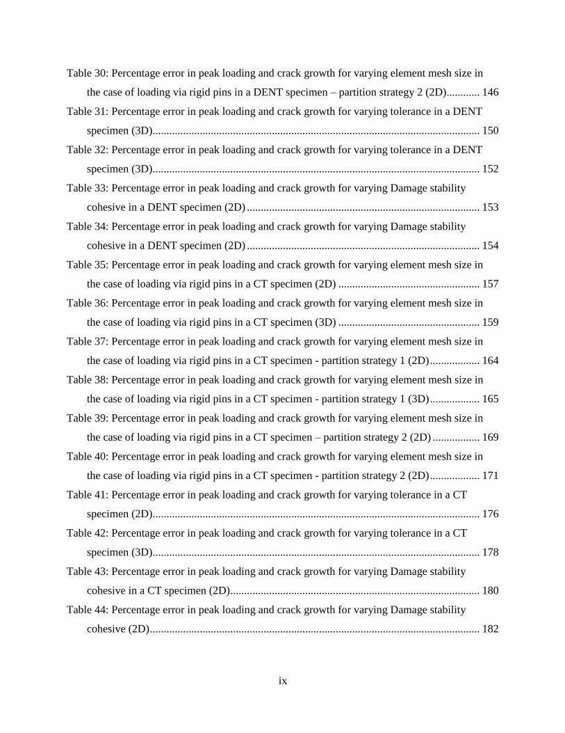
Table 30: Percentage error in peak loading and crack growth for varying element mesh size in
the case of loading via rigid pins in a DENT specimen – partition strategy 2 (2D)............ 146
Table 31: Percentage error in peak loading and crack growth for varying tolerance in a DENT
specimen (3D)...................................................................................................................... 150
Table 32: Percentage error in peak loading and crack growth for varying tolerance in a DENT
specimen (3D)...................................................................................................................... 152
Table 33: Percentage error in peak loading and crack growth for varying Damage stability
cohesive in a DENT specimen (2D) .................................................................................... 153
Table 34: Percentage error in peak loading and crack growth for varying Damage stability
cohesive in a DENT specimen (2D) .................................................................................... 154
Table 35: Percentage error in peak loading and crack growth for varying element mesh size in
the case of loading via rigid pins in a CT specimen (2D) ................................................... 157
Table 36: Percentage error in peak loading and crack growth for varying element mesh size in
the case of loading via rigid pins in a CT specimen (3D) ................................................... 159
Table 37: Percentage error in peak loading and crack growth for varying element mesh size in
the case of loading via rigid pins in a CT specimen - partition strategy 1 (2D) .................. 164
Table 38: Percentage error in peak loading and crack growth for varying element mesh size in
the case of loading via rigid pins in a CT specimen - partition strategy 1 (3D) .................. 165
Table 39: Percentage error in peak loading and crack growth for varying element mesh size in
the case of loading via rigid pins in a CT specimen – partition strategy 2 (2D) ................. 169
Table 40: Percentage error in peak loading and crack growth for varying element mesh size in
the case of loading via rigid pins in a CT specimen - partition strategy 2 (2D) .................. 171
Table 41: Percentage error in peak loading and crack growth for varying tolerance in a CT
specimen (2D)...................................................................................................................... 176
Table 42: Percentage error in peak loading and crack growth for varying tolerance in a CT
specimen (3D)...................................................................................................................... 178
Table 43: Percentage error in peak loading and crack growth for varying Damage stability
cohesive in a CT specimen (2D) .......................................................................................... 180
Table 44: Percentage error in peak loading and crack growth for varying Damage stability
cohesive (2D) ....................................................................................................................... 182
x
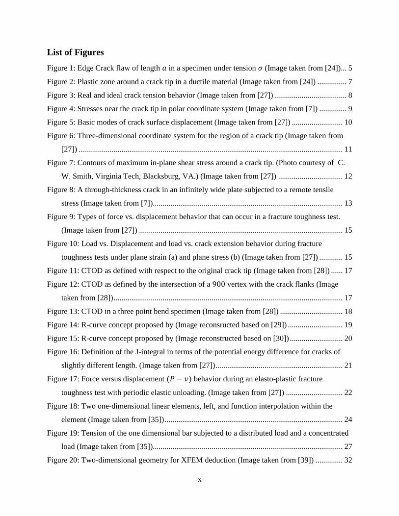
List of Figures
Figure 1: Edge Crack flaw of length 𝑎 in a specimen under tension 𝜎 (Image taken from [24]) ... 5
Figure 2: Plastic zone around a crack tip in a ductile material (Image taken from [24]) ............... 7
Figure 3: Real and ideal crack tension behavior (Image taken from [27]) ..................................... 8
Figure 4: Stresses near the crack tip in polar coordinate system (Image taken from [7]) .............. 9
Figure 5: Basic modes of crack surface displacement (Image taken from [27]) .......................... 10
Figure 6: Three-dimensional coordinate system for the region of a crack tip (Image taken from
[27]) ....................................................................................................................................... 11
Figure 7: Contours of maximum in-plane shear stress around a crack tip. (Photo courtesy of C.
W. Smith, Virginia Tech, Blacksburg, VA.) (Image taken from [27]) ................................. 12
Figure 8: A through-thickness crack in an infinitely wide plate subjected to a remote tensile
stress (Image taken from [7]) ................................................................................................. 13
Figure 9: Types of force vs. displacement behavior that can occur in a fracture toughness test.
(Image taken from [27]) ........................................................................................................ 15
Figure 10: Load vs. Displacement and load vs. crack extension behavior during fracture
toughness tests under plane strain (a) and plane stress (b) (Image taken from [27]) ............ 15
Figure 11: CTOD as defined with respect to the original crack tip (Image taken from [28]) ...... 17
Figure 12: CTOD as defined by the intersection of a 900 vertex with the crack flanks (Image
taken from [28]) ..................................................................................................................... 17
Figure 13: CTOD in a three point bend specimen (Image taken from [28]) ................................ 18
Figure 14: R-curve concept proposed by (Image reconsructed based on [29]) ............................ 19
Figure 15: R-curve concept proposed by (Image reconstructed based on [30]) ........................... 20
Figure 16: Definition of the J-integral in terms of the potential energy difference for cracks of
slightly different length. (Image taken from [27]) ................................................................. 21
Figure 17: Force versus displacement (𝑃 − 𝑣) behavior during an elasto-plastic fracture
toughness test with periodic elastic unloading. (Image taken from [27]) ............................. 22
Figure 18: Two one-dimensional linear elements, left, and function interpolation within the
element (Image taken from [35]) ........................................................................................... 24
Figure 19: Tension of the one dimensional bar subjected to a distributed load and a concentrated
load (Image taken from [35])................................................................................................. 27
Figure 20: Two-dimensional geometry for XFEM deduction (Image taken from [39]) .............. 32
xi
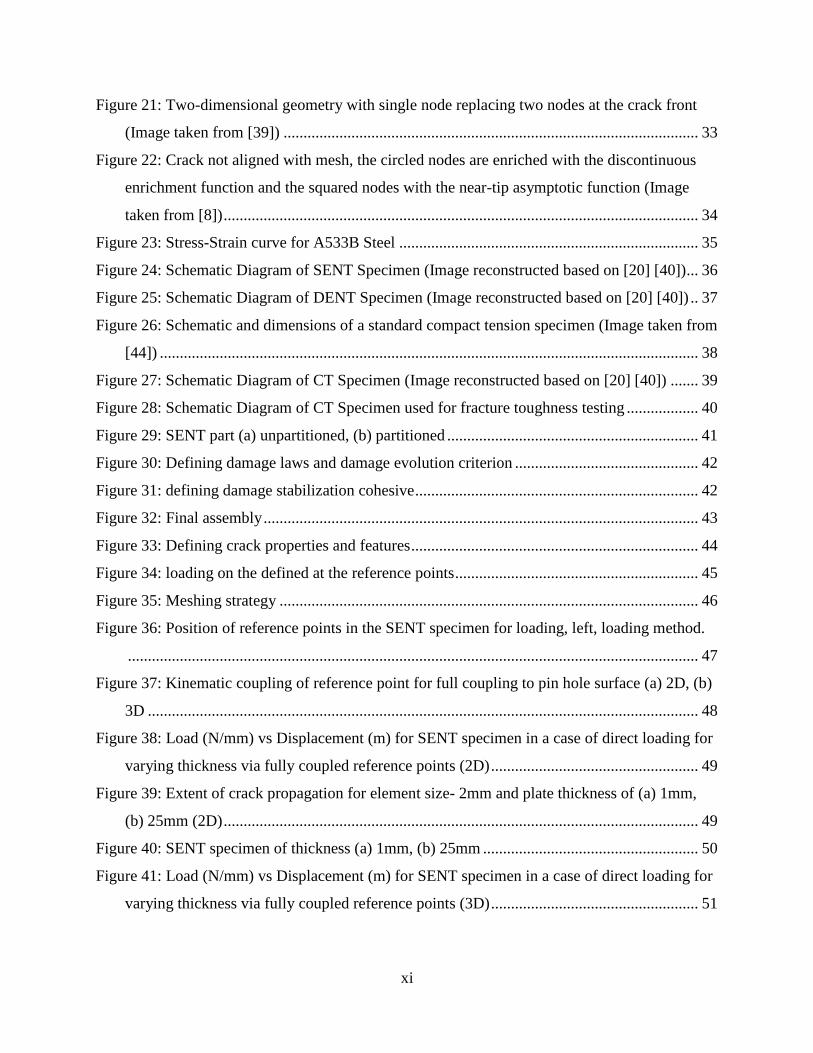
Figure 21: Two-dimensional geometry with single node replacing two nodes at the crack front
(Image taken from [39]) ........................................................................................................ 33
Figure 22: Crack not aligned with mesh, the circled nodes are enriched with the discontinuous
enrichment function and the squared nodes with the near-tip asymptotic function (Image
taken from [8]) ....................................................................................................................... 34
Figure 23: Stress-Strain curve for A533B Steel ........................................................................... 35
Figure 24: Schematic Diagram of SENT Specimen (Image reconstructed based on [20] [40]) ... 36
Figure 25: Schematic Diagram of DENT Specimen (Image reconstructed based on [20] [40]) .. 37
Figure 26: Schematic and dimensions of a standard compact tension specimen (Image taken from
[44]) ....................................................................................................................................... 38
Figure 27: Schematic Diagram of CT Specimen (Image reconstructed based on [20] [40]) ....... 39
Figure 28: Schematic Diagram of CT Specimen used for fracture toughness testing .................. 40
Figure 29: SENT part (a) unpartitioned, (b) partitioned ............................................................... 41
Figure 30: Defining damage laws and damage evolution criterion .............................................. 42
Figure 31: defining damage stabilization cohesive ....................................................................... 42
Figure 32: Final assembly ............................................................................................................. 43
Figure 33: Defining crack properties and features ........................................................................ 44
Figure 34: loading on the defined at the reference points ............................................................. 45
Figure 35: Meshing strategy ......................................................................................................... 46
Figure 36: Position of reference points in the SENT specimen for loading, left, loading method.
............................................................................................................................................... 47
Figure 37: Kinematic coupling of reference point for full coupling to pin hole surface (a) 2D, (b)
3D .......................................................................................................................................... 48
Figure 38: Load (N/mm) vs Displacement (m) for SENT specimen in a case of direct loading for
varying thickness via fully coupled reference points (2D) .................................................... 49
Figure 39: Extent of crack propagation for element size- 2mm and plate thickness of (a) 1mm,
(b) 25mm (2D) ....................................................................................................................... 49
Figure 40: SENT specimen of thickness (a) 1mm, (b) 25mm ...................................................... 50
Figure 41: Load (N/mm) vs Displacement (m) for SENT specimen in a case of direct loading for
varying thickness via fully coupled reference points (3D) .................................................... 51
xii
Figure 42: Extent of crack propagation for element size- 2mm and plate thickness of (a) 1mm,
(b) 25mm (3D) ....................................................................................................................... 52
Figure 43: View of the crack front through the thickness in the specimen of 25mm thickness ... 52
Figure 44: Unstructured Meshing Strategy using Advancing Front Mapped Meshing for (a) 2D,
(b) 3D ..................................................................................................................................... 53
Figure 45: Load (N/mm) vs Displacement (m) for SENT specimen in a case of direct loading for
varying mesh sizes via fully coupled reference points (2D) ................................................. 54
Figure 46: Crack propagation for 2mm element size in case of fully coupled pin-less loading
(2D) ........................................................................................................................................ 55
Figure 47: Variation in crack propagation due to variation in element size in case of fully
coupled pin-less loading (2D)................................................................................................ 55
Figure 48: Load (N/mm) vs Displacement (m) for SENT specimen in a case of direct loading for
varying mesh sizes via fully coupled reference points (3D) ................................................. 57
Figure 49: Crack propagation for 2mm element size in case of fully coupled pin-less loading
(3D) ........................................................................................................................................ 57
Figure 50: Variation in crack propagation due to variation in element size in case of fully
coupled pin-less loading (3D)................................................................................................ 58
Figure 51: Load (N/mm) vs Displacement (m) for SENT specimen for mesh sizes close to 5mm
in a case of direct loading via fully coupled reference points (3D) ....................................... 59
Figure 52: Comparison of Load (N/mm) vs Displacement (m) for 2D and 3D SENT specimen in
a case of direct loading via fully coupled reference points ................................................... 60
Figure 53: Extent of crack propagation for element size- 2mm in (a) 2D, (b) 3D ....................... 60
Figure 54: Load displacement graph comparing element deletion in LS-Dyna against XFEM in
Abaqus in a case of direct loading via fully coupled reference points .................................. 61
Figure 55: Kinematic coupling of reference point for semi coupling to pin hole surface (a) 2D,
(b) 3D ..................................................................................................................................... 62
Figure 56: Load (N/mm) vs Displacement (m) for SENT specimen in a case of direct for varying
mesh sizes loading via semi coupled reference points (2D) .................................................. 63
Figure 57: Crack propagation for 2mm element size in case of semi coupled pin-less loading
(2D) ........................................................................................................................................ 63
xiii
Figure 58: Variation in crack propagation due to variation in element size in case of semi
coupled pin-less loading (2D)................................................................................................ 64
Figure 59: Load (N/mm) vs Displacement (m) for SENT specimen in a case of direct loading for
varying mesh sizes via semi coupled reference points (3D) ................................................. 65
Figure 60: Crack propagation for 3mm element size in case of semi coupled pin-less loading
(3D) ........................................................................................................................................ 66
Figure 61: Variation in crack propagation due to variation in element size in case of semi
coupled pin-less loading (3D)................................................................................................ 66
Figure 62: Comparison of Load (N/mm) vs Displacement (m) for 2D and 3D SENT specimen in
a case of direct loading via semi coupled reference points for varying element sizes of (a)
1mm, (b) 3mm and (c) 4mm .................................................................................................. 67
Figure 63: Extent of crack propagation for 2D (left) and 3D SENT (right) specimen in a case of
direct loading via semi coupled reference points for varying element sizes of (a) 1mm, (b)
3mm and (c) 4mm.................................................................................................................. 68
Figure 64: Rigid body constraint between the reference point and rigid pin in the case of (a) 2D,
(b) 3D ..................................................................................................................................... 69
Figure 65: Load (N/mm) vs Displacement (m) for SENT specimen in a case of loading via rigid
pins for varying mesh sizes (2D) ........................................................................................... 70
Figure 66: Close up of rigid pin during loading (2D) ................................................................... 70
Figure 67: Crack propagation for 2mm element size in case of loading via rigid pins (2D) ........ 71
Figure 68: Variation in crack propagation due to variation in element size in case of loading via
rigid pins (2D) ....................................................................................................................... 71
Figure 69: Load (N/mm) vs Displacement (m) for SENT specimen in a case of loading via rigid
pins for varying mesh sizes (3D) ........................................................................................... 73
Figure 70: Close up of rigid pin during loading (3D) ................................................................... 73
Figure 71: Crack propagation for 2mm element size in case of loading via rigid pins (3D) ........ 74
Figure 72: Variation in crack propagation due to variation in element size in case of loading via
rigid pins (3D) ....................................................................................................................... 74
Figure 73: Comparison of Load (N/mm) vs Displacement (m) for 2D and 3D SENT specimen in
a case of direct loading via rigid pins .................................................................................... 75
xiv
Figure 74: Extent of crack propagation for models of mesh size 2mm in a case of loading via
rigid pins in (a) 2D and (b) 3D .............................................................................................. 76
Figure 75: loading via deformable pin in 2D ................................................................................ 77
Figure 76: Load (N/mm) vs Displacement (m) for SENT specimen in a case of loading via
deformable pins for varying mesh sizes (2D) ........................................................................ 77
Figure 77: Crack propagation for 2mm element size in case of loading via deformable pins (2D)
............................................................................................................................................... 78
Figure 78: Variation in crack propagation due to variation in element size in case of loading via
deformable pins (2D) ............................................................................................................. 78
Figure 79: Loading the deformable pin in 3D .............................................................................. 79
Figure 80: Load (N/mm) vs Displacement (m) for SENT specimen in a case of loading via
deformable pins for varying mesh sizes (3D) ........................................................................ 80
Figure 81: Crack propagation for 2mm element size in case of loading via deformable pins (2D)
............................................................................................................................................... 80
Figure 82: Variation in crack propagation due to variation in element size in case of loading via
deformable pins (3D) ............................................................................................................. 81
Figure 83: Comparison of Load (N/mm) vs Displacement (m) for 2D and 3D SENT specimen in
a case of direct loading via rigid pins .................................................................................... 82
Figure 84: Extent of crack propagation for models of mesh size 2mm in a case of loading via
rigid pins in (a) 2D and (b) 3D .............................................................................................. 82
Figure 85; Plastic zone shapes according to von Mises and Tresca yield criteria (a) von Mises
criterion , (b) Tresca criterion [46] ........................................................................................ 83
Figure 86: Plastic strain contours showing plastic zone shape at the crack tip in (a) plane strain
model, (b) plane stress model ................................................................................................ 83
Figure 87: Plastic strain contours showing plastic zone shape at the crack tip in a 3D model ..... 84
Figure 88: Stress-Strain behavior (a) Linear Elastic Fracture (LEF), ........................................... 85
Figure 89: Load-displacement behavior for variation in fracture mechanic in the case of a fully
coupled pin-less loading, 2mm (2D) ..................................................................................... 85
Figure 90: Crack Propagation - Stress distribution (a) Linear Elastic Fracture (LEF), (b) Elastic
Plastic Fracture (EPF), (c) Linear Elastic Linear Plastic Fracture (LELPF) (2D) ................ 86
xv
Figure 91: Load-displacement behavior for variation in fracture mechanic in the case of a fully
coupled pin-less loading, 2mm (3D) ..................................................................................... 87
Figure 92: Crack Propagation - Stress distribution (a) Linear Elastic Fracture (LEF), (b) Elastic
Plastic Fracture (EPF), (c) Linear Elastic Linear Plastic Fracture (LELPF) (3D) ................ 88
Figure 93: Deviation in the crack growth in a case of LEF .......................................................... 88
Figure 94: Load-displacement behavior for variation in fracture mechanic in the case of loading
via rigid pins, 2mm (2D) ....................................................................................................... 90
Figure 95: Crack Propagation - Stress distribution (a) Linear Elastic Fracture (LEF), (b) Elastic
Plastic Fracture (EPF), (c) Linear Elastic Linear Plastic Fracture (LELPF) (2D) ................ 90
Figure 96: Load-displacement behavior for variation in fracture mechanic in the case of loading
via rigid pins, 2mm (3D) ....................................................................................................... 91
Figure 97: Crack Propagation - Stress distribution (a) Linear Elastic Fracture (LEF), ................ 92
Figure 98: Partitioning strategy 1 (a) 2D, (b) 3D and (c) after meshing ...................................... 93
Figure 99: Load (N/mm) vs Displacement (m) for SENT specimen in a case of loading via rigid
pins for varying mesh sizes using partitioning strategy 1 (2D) ............................................. 94
Figure 100: Variation in crack propagation due to variation in element size in case of loading via
rigid pins using partitioning strategy 1 (2D) ......................................................................... 95
Figure 101: Deviation in initial crack (a) without visible mesh, (b) with visible mesh ............... 95
Figure 102: Load (N/mm) vs Displacement (m) for SENT specimen in a case of loading via rigid
pins for varying mesh sizes using partitioning strategy 1 (3D) ............................................. 96
Figure 103: Variation in crack propagation due to variation in element size in case of loading via
rigid pins using partitioning strategy 1 (2D) ......................................................................... 97
Figure 104: Extent of crack propagation for element size- 1mm in (a) 2D, (b) 3D ..................... 98
Figure 105: Comparison of Load (N/mm) vs Displacement (m) for 2D and 3D SENT specimen
in a case of via deformable pins for partition strategy 1 ....................................................... 98
Figure 106: pin-hole deformation causing it to overlap itself....................................................... 99
Figure 107: Initial crack starts between two elements .................................................................. 99
Figure 108: Load (N/mm) vs Displacement (m) for SENT specimen in a case of loading via
deformable pins for varying mesh sizes using partitioning strategy 1 (2D) ........................ 100
Figure 109: Variation in crack propagation due to variation in element size in case of loading via
rigid pins using partitioning strategy 1 (2D) ....................................................................... 101
xvi
Figure 110: (a) Load-displacement graph showing a kink just as loading begins, (b) overlapping
of pin and plate causing the kink in the graph ..................................................................... 102
Figure 111: Load (N/mm) vs Displacement (m) for SENT specimen in a case of loading via
deformable pins for varying mesh sizes using partitioning strategy 1 (3D) ........................ 102
Figure 112: Variation in crack propagation due to variation in element size in case of loading via
rigid pins using partitioning strategy 1 (3D) ....................................................................... 103
Figure 113: Comparison of Load (N/mm) vs Displacement (m) for 2D and 3D SENT specimen
in a case of via deformable pins for partition strategy 1 ..................................................... 104
Figure 114: Partitioning Strategy 2 (a) 2D, (b) 3D ..................................................................... 105
Figure 115: Meshing for partitioning strategy 2 ......................................................................... 105
Figure 116: Load (N/mm) vs Displacement (m) for SENT specimen in a case of loading via rigid
pins for varying mesh sizes using partitioning strategy 2 (2D) ........................................... 106
Figure 117: Variation in crack propagation due to variation in element size in case of loading via
rigid pins using partitioning strategy 2 (2D) ....................................................................... 107
Figure 118: Load (N/mm) vs Displacement (m) for SENT specimen in a case of loading via rigid
pins for varying mesh sizes using partitioning strategy 2 (3D) ........................................... 108
Figure 119: Variation in crack propagation due to variation in element size in case of loading via
rigid pins using partitioning strategy 2 (3D) ....................................................................... 109
Figure 120: Comparison of Load (N/mm) vs Displacement (m) for 2D and 3D SENT specimen
in a case of loading via rigid pins for partition strategy 2 ................................................... 110
Figure 121: Comparison of crack extent for (a) 2D and (b) 3D SENT specimen in a case of
loading via rigid pins for partition strategy 2 ...................................................................... 110
Figure 122: Load (N/mm) vs Displacement (m) for SENT specimen in a case of loading via
deformable pins for varying mesh sizes using partitioning strategy 2 (2D) ........................ 111
Figure 123: Variation in crack propagation due to variation in element size in case of loading via
deformable pins using partitioning strategy 2 (2D) ............................................................. 112
Figure 124: Load (N/mm) vs Displacement (m) for SENT specimen in a case of loading via
deformable pins for varying mesh sizes using partitioning strategy 2 (3D) ........................ 113
Figure 125: Variation in crack propagation due to variation in element size in case of loading via
deformable pins using partitioning strategy 2 (3D) ............................................................. 114
xvii
Figure 126: Comparison of Load (N/mm) vs Displacement (m) for 2D and 3D SENT specimen
in a case of loading via rigid pins for partition strategy 2 ................................................... 115
Figure 127: Comparison of crack extent for (a) 2D and (b) 3D SENT specimen in a case of
loading via deformable pins for partition strategy 2............................................................ 116
Figure 128: Comparison of Load vs Displacement for 2D SENT specimen for varying element
type ...................................................................................................................................... 117
Figure 129: Comparison of crack growth extent for 2D SENT specimen for varying element
types ..................................................................................................................................... 118
Figure 130: Large stresses developing at the pin holes in CPS4 ................................................ 118
Figure 131: Comparison of Load vs Displacement for 3D SENT specimen for varying element
type ...................................................................................................................................... 120
Figure 132: Comparison of crack growth extent for 3D SENT specimen for varying element
types ..................................................................................................................................... 120
Figure 133: (a) Comparison of Load vs Displacement and (b) stress contours for 2D SENT
specimen for varying tolerance ............................................................................................ 122
Figure 134: Comparison of Load vs Displacement for 3D SENT specimen for varying tolerance
............................................................................................................................................. 122
Figure 135: Comparison of crack growth extent for 3D SENT specimen for varying tolerance 123
Figure 136: Comparison of Load vs Displacement for 3D SENT specimen for varying tolerance
at low mesh densities ........................................................................................................... 124
Figure 137: Comparison of Load vs Displacement for 2D SENT specimen for varying tolerance
............................................................................................................................................. 125
Figure 138: Comparison of crack growth extent for 2D SENT specimen for varying damage
stability cohesive ................................................................................................................. 125
Figure 139: Comparison of Load vs Displacement for 3D SENT specimen for varying damage
stability cohesive ................................................................................................................. 126
Figure 140: Comparison of crack growth extent for 3D SENT specimen for varying damage
stability cohesive ................................................................................................................. 127
Figure 141: Comparison of Load vs Displacement for 3D SENT specimen for varying damage
stability cohesive between 2e-4 and 2e-3 ............................................................................ 128
xviii
Figure 142: Comparison of crack growth extent for 3D SENT specimen for varying damage
stability cohesive between 2e-4 and 2e-3 ............................................................................ 128
Figure 143: Approximation of SENT specimen for Stress intensity factor calculation ............. 129
Figure 144: Load (N/mm) vs Displacement (m) for DENT specimen in a case of loading via rigid
pins for varying mesh sizes (2D) ......................................................................................... 131
Figure 145: Overlapping of pin hole surface .............................................................................. 132
Figure 146: Variation in crack propagation due to variation in element size in case of loading via
rigid pins (2D) ..................................................................................................................... 132
Figure 147: Load (N/mm) vs Displacement (m) for DENT specimen in a case of loading via rigid
pins for varying mesh sizes (3D) ......................................................................................... 133
Figure 148: Crack failing to initiate at the edge of the specimen in the high density mesh ....... 134
Figure 149: Variation in crack propagation due to variation in element size in case of loading via
rigid pins (3D) ..................................................................................................................... 134
Figure 150: Comparison of Load (N/mm) vs Displacement (m) for 2D and 3D DENT specimen
in a case of loading via rigid pins ........................................................................................ 135
Figure 151: Comparison of crack extent for (a) 2D and (b) 3D DENT specimen in a case of
loading via rigid pins ........................................................................................................... 136
Figure 152: (a) Partition strategy 1 for DENT specimen, (b) Meshing strategy ........................ 137
Figure 153: Load (N/mm) vs Displacement (m) for CT specimen in a case of loading via rigid
pins for varying mesh sizes and partition strategy 1 (2D) ................................................... 137
Figure 154: Unnatural initial crack at the boundary of two rows of elements ........................... 138
Figure 155: Variation in crack propagation due to variation in element size in case of loading via
rigid pins using partitioning strategy 1 (2D) ....................................................................... 138
Figure 156: Load (N/mm) vs Displacement (m) for CT specimen in a case of loading via rigid
pins for varying mesh sizes and partition strategy 1 (3D) ................................................... 140
Figure 157: Variation in crack propagation due to variation in element size in case of loading via
rigid pins using partitioning strategy 1 (2D) ....................................................................... 141
Figure 158: Comparison of Load (N/mm) vs Displacement (m) for 2D and 3D DENT specimen
in a case of loading via rigid pins ........................................................................................ 142
Figure 159: Comparison of crack extent for (a) 2D and (b) 3D DENT specimen in a case of
loading via rigid pins ........................................................................................................... 142
xix
Figure 160: (a) Partition strategy 2 for DENT specimen, (b) Meshing strategy ........................ 143
Figure 161: Load (N/mm) vs Displacement (m) for CT specimen in a case of loading via rigid
pins for varying mesh sizes and partition strategy 2 (2D) ................................................... 143
Figure 162: Variation in crack propagation due to variation in element size in case of loading via
rigid pins using partitioning strategy 2 (2D) ....................................................................... 144
Figure 163: Load (N/mm) vs Displacement (m) for CT specimen in a case of loading via rigid
pins for varying mesh sizes and partition strategy 2 (3D) ................................................... 145
Figure 164: Variation in crack propagation due to variation in element size in case of loading via
rigid pins using partitioning strategy 2 (3D) ....................................................................... 146
Figure 165: Load-displacement behavior for variation in fracture mechanic in the DENT
specimen, (2D)..................................................................................................................... 147
Figure 166: Crack Propagation - Stress distribution (a) Linear Elastic Fracture (LEF), (b) Elastic
Plastic Fracture (EPF), (c) Linear Elastic Linear Plastic Fracture (LELPF) (2D) .............. 148
Figure 167: Load-displacement behavior for variation in fracture mechanic in the DENT
specimen, (3D)..................................................................................................................... 148
Figure 168: Crack Propagation - Stress distribution (a) Linear Elastic Fracture (LEF), (b) Elastic
Plastic Fracture (EPF), (c) Linear Elastic Linear Plastic Fracture (LELPF) (2D) .............. 149
Figure 169: (a) Comparison of Load vs Displacement and (b) stress contours for 2D DENT
specimen for varying tolerance ............................................................................................ 149
Figure 170: (a) Comparison of Load vs Displacement for 3D DENT specimen for varying
tolerance ............................................................................................................................... 151
Figure 171: Comparison of crack growth extent for 3D DENT specimen for varying tolerance
............................................................................................................................................. 151
Figure 172: (a) Comparison of Load vs Displacement and (b) stress contours for 2D DENT
specimen for varying Damage Stability Cohesive .............................................................. 152
Figure 173: Comparison of Load vs Displacement for 3D DENT specimen for varying Damage
Stability Cohesive ................................................................................................................ 153
Figure 174: Comparison of crack growth extent for 3D DENT specimen for varying tolerance
............................................................................................................................................. 154
Figure 175: Approximation of SENT specimen for Stress intensity factor calculation ............. 155
xx
Figure 176: Load (N/mm) vs Displacement (m) for CT specimen in a case of loading via rigid
pins for varying mesh sizes (2D) ......................................................................................... 156
Figure 177: Crack propagation for 2mm element size in case of loading via rigid pins in CT
specimen (2D)...................................................................................................................... 157
Figure 178: Variation in crack propagation due to variation in element size in case of loading via
rigid pins (2D) ..................................................................................................................... 157
Figure 179: Load (N/mm) vs Displacement (m) for CT specimen in a case of loading via rigid
pins for varying mesh sizes (3D) ......................................................................................... 158
Figure 180: Crack propagation for 2mm element size in case of loading via rigid pins in CT
specimen (3D)...................................................................................................................... 159
Figure 181: Variation in crack propagation due to variation in element size in case of loading via
rigid pins (3D) ..................................................................................................................... 159
Figure 182: Comparison of Load (N/mm) vs Displacement (m) for 2D and 3D CT specimen in a
case of loading via rigid pins ............................................................................................... 160
Figure 183: Comparison of crack extent for (a) 2D and (b) 3D CT specimen in a case of loading
via rigid pins ........................................................................................................................ 161
Figure 184: Partitioning strategy (a) in 2D and 3D, (b) meshing strategy ................................. 162
Figure 185: Load (N/mm) vs Displacement (m) for CT specimen in a case of loading via rigid
pins for varying mesh sizes and partition strategy 1 (2D) ................................................... 162
Figure 186: Variation in crack propagation due to variation in element size in case of loading via
rigid pins using partitioning strategy 1 (2D) ....................................................................... 163
Figure 187: Load (N/mm) vs Displacement (m) for CT specimen in a case of loading via rigid
pins for varying mesh sizes and partition strategy 1 (3D) ................................................... 164
Figure 188: Variation in crack propagation due to variation in element size in case of loading via
rigid pins using partitioning strategy 1 (3D) ....................................................................... 165
Figure 189: Comparison of Load (N/mm) vs Displacement (m) for 2D and 3D CT specimen in a
case of loading via rigid pins for partition strategy 1 .......................................................... 166
Figure 190: Comparison of crack extent for (a) 2D and (b) 3D CT specimen in a case of loading
via rigid pins for partition strategy 1 ................................................................................... 166
Figure 191: Partitioning strategy (a) in 2D and 3D, (b) meshing strategy ................................. 167
xxi
Figure 192: Load (N/mm) vs Displacement (m) for CT specimen in a case of loading via rigid
pins for varying mesh sizes and partition strategy 2 (2D) ................................................... 168
Figure 193: Variation in crack propagation due to variation in element size in case of loading via
rigid pins using partitioning strategy 2 (2D) ....................................................................... 168
Figure 194: Load (N/mm) vs Displacement (m) for CT specimen in a case of loading via rigid
pins for varying mesh sizes and partition strategy 2 (3D) ................................................... 169
Figure 195: Variation in crack propagation due to variation in element size in case of loading via
rigid pins using partitioning strategy 2 (3D) ....................................................................... 170
Figure 196: Comparison of Load (N/mm) vs Displacement (m) for 2D and 3D CT specimen in a
case of loading via rigid pins for partition strategy 1 .......................................................... 171
Figure 197: Comparison of crack extent for (a) 2D and (b) 3D CT specimen in a case of loading
via rigid pins for partition strategy 2 ................................................................................... 172
Figure 198: Load-displacement behavior for variation in fracture mechanic in the CT specimen,
(2D) ...................................................................................................................................... 173
Figure 199: Crack Propagation - Stress distribution (a) Linear Elastic Fracture (LEF), (b) Elastic
Plastic Fracture (EPF), (c) Linear Elastic Linear Plastic Fracture (LELPF) (2D) .............. 173
Figure 200: Load-displacement behavior for variation in fracture mechanic in the CT specimen,
(3D) ...................................................................................................................................... 174
Figure 201: Crack Propagation - Stress distribution (a) Linear Elastic Fracture (LEF), (b) Elastic
Plastic Fracture (EPF), (c) Linear Elastic Linear Plastic Fracture (LELPF) (3D) .............. 174
Figure 202: Comparison of Load vs Displacement for 2D CT specimen for varying tolerance 175
Figure 203: Comparison of crack growth extent for 2D CT specimen for varying tolerance .... 176
Figure 204: Comparison of Load vs Displacement for 3D CT specimen for varying tolerance 177
Figure 205: Comparison of crack growth extent for 3D CT specimen for varying tolerance .... 178
Figure 206: Comparison of Load vs Displacement for 2D CT specimen for varying Damage
Stability Cohesive ................................................................................................................ 179
Figure 207: Comparison of crack growth extent for 2D CT specimen for varying Damage
Stability Cohesive ................................................................................................................ 180
Figure 208: Comparison of Load vs Displacement for 3D CT specimen for varying Damage
Stability Cohesive ................................................................................................................ 181
xxii
Figure 209: Comparison of crack growth extent for 3D CT specimen for varying Damage
Stability Cohesive ................................................................................................................ 181
Figure 210: Reduction in area at the crack tip ............................................................................ 182
Figure 211: Eccentric loading of a plate with an edge crack, and the superposition used to obtain
K. ......................................................................................................................................... 183
Figure 212: Comparison of 2D and 3D load-displacement data................................................. 184
Figure 213: Extent of crack growth and stress contours in (a) 2D and (b) 3D ........................... 185
Figure 214: Load-displacement data for CT specimen for varying mesh size ........................... 186
Figure 215: Crack extent and stress contours for CT specimen for varying mesh size .............. 186
Figure 216: Load-displacement data for CT specimen showing the effect of Non-linear geometry
............................................................................................................................................. 187
Figure 217: Crack extent and stress contours for CT specimen for (a) NLGeom turned off and
(b) NLGeom turned on ........................................................................................................ 187
Figure 218: Load-displacement data for CT specimen showing the effect of Non-linear geometry
............................................................................................................................................. 188
Figure 219: Crack extent and stress contours for CT specimen for (a) NLGeom turned off and
(b) NLGeom turned on ........................................................................................................ 188
Figure 220: Load-displacement data for CT specimen for varying Damage stability cohesive . 189
Figure 221: Crack extent and stress contours for CT specimen varying Damage stability cohesive
............................................................................................................................................. 189
Figure 222: (a) Load-displacement data for CT specimen and (b) stress contours and crack
growth extent for thickness of 3.1mm ................................................................................. 190
Figure 223: (a) Load-displacement data for CT specimen and (b) stress contours and crack
growth extent for thickness of 6.35mm ............................................................................... 191
Figure 224: (a) Load-displacement data for CT specimen and (b) stress contours and crack
growth extent for thickness of 19.1mm using plane stress formulation .............................. 191
Figure 225: (a) Load-displacement data for CT specimen and (b) stress contours and crack
growth extent for thickness of 19.1mm using plane strain formulation .............................. 192
Figure 226: In-plane shear stress contours (a) in the entire SENT model, (b) at the crack tip ... 192
Figure 227: (a) Contours of maximum in-plane shear stress around a crack tip (Image taken from
[27]), (b) maximum in plane shear stress in the 3D SENT specimen ................................. 193
xxiii
Figure 228: Strain energy density plot (a) in the 3D SENT model, (b) at the crack tip ............. 194
Figure 229: In-plane shear stress contours (a) in the entire DENT model, (b) at the crack tip .. 194
Figure 230: Strain energy density plot (a) in the 3D SENT model, (b) at the crack tip ............. 195
Figure 231: In-plane shear stress contours (a) in the entire CT model, (b) at the crack tip ........ 195
Figure 232: Shear stress observed at contact points in the cracked plate ................................... 196
Figure 233: Strain energy density plot (a) in the CT model, (b) at the crack tip ........................ 196
Figure 234: Load-displacement data for 3D SENT specimen of element mesh size 1mm for
varying tolerance at damage stability cohesive of (a) 2e-4 and (b) 2e-3 ............................. 204
Figure 235: Load-displacement data for 3D SENT specimen of element mesh size 2mm for
varying tolerance at damage stability cohesive of (a) 2e-4 and (b) 2e-3 ............................. 205
Figure 236: Load-displacement data for 3D CT specimen of element mesh size 1mm for varying
tolerance at damage stability cohesive of (a) 2e-4 and (b) 2e-3 .......................................... 205
Figure 237: Load-displacement data for 3D CT specimen of element mesh size 2mm for varying
tolerance at damage stability cohesive of (a) 2e-4 and (b) 2e-3 .......................................... 206
Figure 238: Load-displacement data for 3D CT specimen for varying matrix storage method
using (a) a direct solver and (b) an iterative solver ............................................................. 206
Figure 239: (a) Load-displacement data and (b) stress contours for 2D SENT specimen for
NLGeom turned on and off ................................................................................................. 207
Figure 240: (a) Load-displacement data and (b) stress contours for 3D SENT specimen for
NLGeom turned on and off ................................................................................................. 208
Figure 241: (a) Load-displacement data and (b) stress contours for 2D DENT specimen for
NLGeom turned on and off ................................................................................................. 208
Figure 242: (a) Load-displacement data and (b) stress contours for 3D DENT specimen for
NLGeom turned on and off ................................................................................................. 209
Figure 243: (a) Load-displacement data and (b) stress contours for 2D CT specimen for NLGeom
turned on and off.................................................................................................................. 209
Figure 244: (a) Load-displacement data and (b) stress contours for 3D CT specimen for NLGeom
turned on and off.................................................................................................................. 210
xxiv
Thesis Map
This thesis aims to provide a better understanding to the features and parametric dependencies of
XFEM crack growth in quasi-static tension. A thorough description of the simulations conducted
is presented. It covers various parameters including meshing strategy, loading strategy, and
tolerance. The work done is organized as follows.
Chapter 1- This chapter introduces of concepts of failure and the need that lead to the inception
of XFEM. This chapter also outlines the objectives of the thesis.
Chapter 2- Description of the theory behind fracture, finite element analysis and XFEM.
Chapter 3- Description of the experiments and the material models for the specimens simulated
in the thesis.
Chapter 4- Approach used to model crack growth using XFEM in Abaqus is described in this
section.
Chapter 5- Parametric analysis, providing a better understanding of how variations in each
parameter can affect the performance of the simulation.
Chapter 6- Discussion of results from the parametric analysis and the drawing of conclusions
from the results.
Contributions and future work
1
1. Introduction
1.1. Context
In the present day, the review and assessment of the trustworthiness of the different mechanical
segments is greatly essential for the Industry. The two noteworthy objectives are: Increase in
fatigue life expectancy, what's more, their safety.
Until recently, lengthy and expensive laboratory experiments were the only way to go about study
and analysis of structural integrity. While they were a medium to predict operating life they
couldn’t be used to determine fracture mechanics properties such as stress intensity factor K [1] .
These tests also have a standard set of rules which need to be followed to obtain viable results
making them tedious to implement [2].
The need for a numerical method to provide a more precise and systematic solution gave rise to
the initial stirrings of the finite element method in the early 1940s. Two of the initial sources
being Alexander Hrennikoff [3] and R Courant [4].
From [3] we learn that he was the first to develop a lattice analogy to solve structural engineering
problems. This lattice analogy is equivalent to the division of structures in to elements in modern
finite element analysis. This contribution would however go unnoticed due to the lack of
computational power to solve such a large system of equations.
Courant [4] introduced the concept of variational methods to solve structural problems. The
concept of a free problem and natural boundary condition are explained. He also explained the
concept of initial and final boundary conditions and also the significance of various types of
boundary conditions such as clamped and pinned. He explained the usage of the Raleigh-Ritz
method [5] to solve variational problems.
Certain mechanical phenomena are difficult to model using Finite Element Method (FEM), which
includes study of stationary cracks and crack propagation. This study would greatly help with the
understanding if mechanical behavior of components as well as to estimate and possibly increase
its life expectancy. Finite element models of adhesively bonded joints and mechanically fastened
joints of an aircraft structure were developed to accurately simulate the nonlinear behavior of
impact loading on pre-strained joints. These models were developed by Binnamangala and
2
Bayandor [6] and provided an understanding into the behavior of pre-strained joints under impact
loading.
There was always a need to accurately represent crack initiation and propagation in mechanical
systems. However a major drawback to using classical FEM in order to solve problems with such
discontinuities is the need to attain a suitable mesh as well as remeshing [7].
In 1999 a numerical technique based on Generalized Finite Element Method (GFEM) and Partition
of Unity Method (PUM) was developed by Ted Belytschko and collaborators known as Extended
Finite Element Method (XFEM) [8]. Extended Finite Element Analysis by Zhuang et al. [9] is a
textbook providing great information regarding XFEM formulation as well as modelling
approaches to various scenarios. This textbook gives us a greater understanding of the underlying
mathematics rather than the actual simulating procedure. A study conducted by Behroozinia et al.
[10] gives us an understanding into the behavior of XFEM crack propagation at the interface of a
biomaterial model. This study used a combination of XFEM and cohesive zone modeling (CZM).
A larger scale version of this implementation of XFEM and CZM is provided by Vigueras et al.
[11]. A method to simulate delamination and self-similar crack growth by employing virtual crack
closure technique (VCCT) in composites modelled using shell layers connected by user-defined
multi-point constraints (MPCs) is illustrated in [12]. The modeling of damage under dynamic
loading at a micro scale in composite laminates is shown in [13]. The concept of delamination and
buckling in thin walled composite shell structures is modeled in [14]. Damage in Glass fiber-
reinforced polymer (GFRP) under tension was simulated and certain convergence issues during
simulation were discussed in [15]. A comparison of XFEM and strain energy approach to evaluate
stress intensity factor at a notch is illustrated in [16]. A new enrichment defined as a Heaviside
function which is stabilized by its linear interpolant which improved the stability of the XFEM
formulation was proposed by [17] in 2015. Similar improvements were made to overcome the
challenge to obtain a direct extension of the singular crack tip enrichment to dynamic/time
dependent problems in [18].
1.2. Objective
XFEM, although a relatively recent concept [8], is now available in commercial versions of finite
element codes. In fact, XFEM has been already implemented in the Finite Element Method
software Abaqus Standard, owned by Simulia [19].
3
A large number of parameters affect crack growth using XFEM. The scope of this work however
would be limited to gaining an understanding of meshing strategy, partitioning, plasticity,
tolerance and damage stability cohesive. There is a need to understand the potential of XFEM in
accurately representing fracture.
A parametric analysis is to be conducted to validate the ability of XFEM to model a real life
structural experiment. A set of three experiments will be used for this validation [20]. The
experiments consist of specimens that are subjected to tension on a Universal Testing Machine
(UTM) by means of pins that pass through holes present in the specimens.
The experiments are differentiated from each other on the basis of the position of the initial crack,
the number of initial cracks and the position of the loading pins. The three specimens in question
are the Single Edge Notch Tension (SENT) specimen having a single notch at the center of one of
the edges and is loaded through the center of the specimen, the Double Edge Notch Tension
(DENT) specimen having a two notches at the center of opposite edges and is loaded through the
center of the specimen, the Compact Tension (CT) having a single notch at the center of one of
the edges and is loaded offset from the center in the direction of crack in the specimen.
The main objectives of this thesis will be to understand the most effective method of modeling
with XFEM and to achieve a model of the highest precision with respect to experimentally
predicted. Hence some simulations will be performed, with solutions known by the scientific
community [20], using Abaqus’ XFEM. With the understanding gained from these simulations an
attempt is made to model the CT specimen used in fracture toughness testing provided in [21].
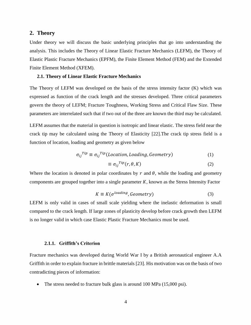
4
2. Theory
Under theory we will discuss the basic underlying principles that go into understanding the
analysis. This includes the Theory of Linear Elastic Fracture Mechanics (LEFM), the Theory of
Elastic Plastic Fracture Mechanics (EPFM), the Finite Element Method (FEM) and the Extended
Finite Element Method (XFEM).
2.1. Theory of Linear Elastic Fracture Mechanics
The Theory of LEFM was developed on the basis of the stress intensity factor (K) which was
expressed as function of the crack length and the stresses developed. Three critical parameters
govern the theory of LEFM; Fracture Toughness, Working Stress and Critical Flaw Size. These
parameters are interrelated such that if two out of the three are known the third may be calculated.
LEFM assumes that the material in question is isotropic and linear elastic. The stress field near the
crack tip may be calculated using the Theory of Elasticity [22].The crack tip stress field is a
function of location, loading and geometry as given below
𝜎𝑖𝑗𝑇𝑖𝑝 ≡ 𝜎𝑖𝑗
𝑇𝑖𝑝(𝐿𝑜𝑐𝑎𝑡𝑖𝑜𝑛, 𝐿𝑜𝑎𝑑𝑖𝑛𝑔, 𝐺𝑒𝑜𝑚𝑒𝑡𝑟𝑦) (1)
≡ 𝜎𝑖𝑗𝑇𝑖𝑝(𝑟, 𝜃, 𝐾) (2)
Where the location is denoted in polar coordinates by 𝑟 and 𝜃, while the loading and geometry
components are grouped together into a single parameter 𝐾, known as the Stress Intensity Factor
𝐾 ≡ 𝐾(𝜎𝑙𝑜𝑎𝑑𝑖𝑛𝑔, 𝐺𝑒𝑜𝑚𝑒𝑡𝑟𝑦) (3)
LEFM is only valid in cases of small scale yielding where the inelastic deformation is small
compared to the crack length. If large zones of plasticity develop before crack growth then LEFM
is no longer valid in which case Elastic Plastic Fracture Mechanics must be used.
2.1.1. Griffith’s Criterion
Fracture mechanics was developed during World War I by a British aeronautical engineer A.A
Griffith in order to explain fracture in brittle materials [23]. His motivation was on the basis of two
contradicting pieces of information:
The stress needed to fracture bulk glass is around 100 MPa (15,000 psi).
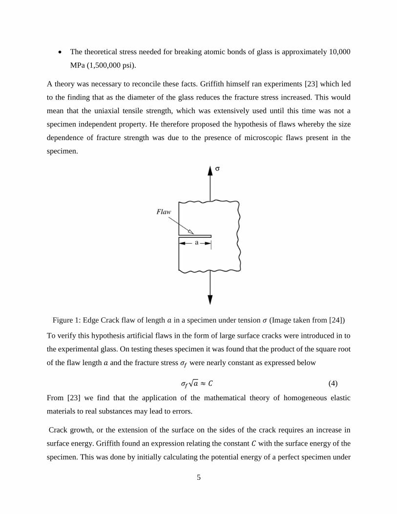
5
The theoretical stress needed for breaking atomic bonds of glass is approximately 10,000
MPa (1,500,000 psi).
A theory was necessary to reconcile these facts. Griffith himself ran experiments [23] which led
to the finding that as the diameter of the glass reduces the fracture stress increased. This would
mean that the uniaxial tensile strength, which was extensively used until this time was not a
specimen independent property. He therefore proposed the hypothesis of flaws whereby the size
dependence of fracture strength was due to the presence of microscopic flaws present in the
specimen.
Figure 1: Edge Crack flaw of length 𝑎 in a specimen under tension 𝜎 (Image taken from [24])
To verify this hypothesis artificial flaws in the form of large surface cracks were introduced in to
the experimental glass. On testing theses specimen it was found that the product of the square root
of the flaw length 𝑎 and the fracture stress 𝜎𝑓 were nearly constant as expressed below
𝜎𝑓√𝑎 ≈ 𝐶 (4)
From [23] we find that the application of the mathematical theory of homogeneous elastic
materials to real substances may lead to errors.
Crack growth, or the extension of the surface on the sides of the crack requires an increase in
surface energy. Griffith found an expression relating the constant 𝐶 with the surface energy of the
specimen. This was done by initially calculating the potential energy of a perfect specimen under
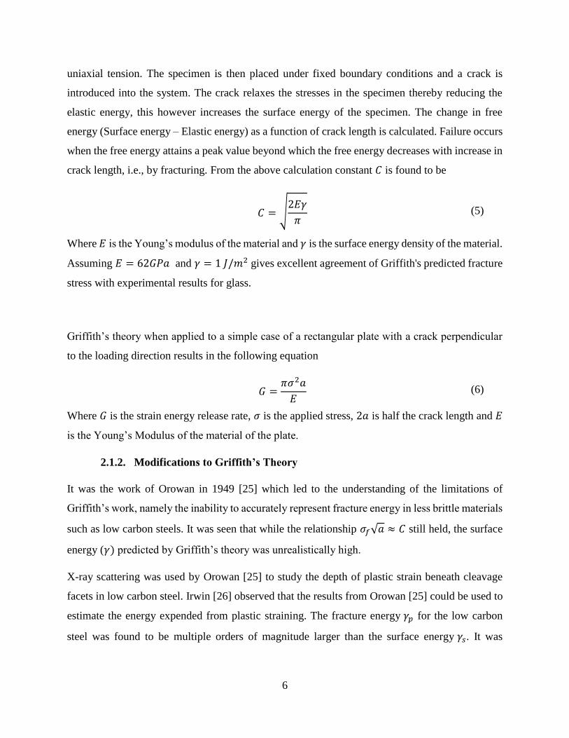
6
uniaxial tension. The specimen is then placed under fixed boundary conditions and a crack is
introduced into the system. The crack relaxes the stresses in the specimen thereby reducing the
elastic energy, this however increases the surface energy of the specimen. The change in free
energy (Surface energy – Elastic energy) as a function of crack length is calculated. Failure occurs
when the free energy attains a peak value beyond which the free energy decreases with increase in
crack length, i.e., by fracturing. From the above calculation constant 𝐶 is found to be
𝐶 = √2𝐸𝛾
𝜋 (5)
Where 𝐸 is the Young’s modulus of the material and 𝛾 is the surface energy density of the material.
Assuming 𝐸 = 62𝐺𝑃𝑎 and 𝛾 = 1 𝐽/𝑚2 gives excellent agreement of Griffith's predicted fracture
stress with experimental results for glass.
Griffith’s theory when applied to a simple case of a rectangular plate with a crack perpendicular
to the loading direction results in the following equation
𝐺 =𝜋𝜎2𝑎
𝐸 (6)
Where 𝐺 is the strain energy release rate, 𝜎 is the applied stress, 2𝑎 is half the crack length and 𝐸
is the Young’s Modulus of the material of the plate.
2.1.2. Modifications to Griffith’s Theory
It was the work of Orowan in 1949 [25] which led to the understanding of the limitations of
Griffith’s work, namely the inability to accurately represent fracture energy in less brittle materials
such as low carbon steels. It was seen that while the relationship 𝜎𝑓√𝑎 ≈ 𝐶 still held, the surface
energy (𝛾) predicted by Griffith’s theory was unrealistically high.
X-ray scattering was used by Orowan [25] to study the depth of plastic strain beneath cleavage
facets in low carbon steel. Irwin [26] observed that the results from Orowan [25] could be used to
estimate the energy expended from plastic straining. The fracture energy 𝛾𝑝 for the low carbon
steel was found to be multiple orders of magnitude larger than the surface energy 𝛾𝑠. It was
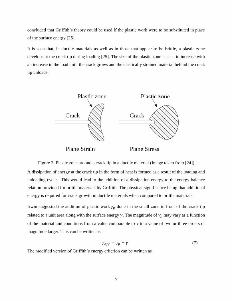
7
concluded that Griffith’s theory could be used if the plastic work were to be substituted in place
of the surface energy [26].
It is seen that, in ductile materials as well as in those that appear to be brittle, a plastic zone
develops at the crack tip during loading [25]. The size of the plastic zone is seen to increase with
an increase in the load until the crack grows and the elastically strained material behind the crack
tip unloads.
Figure 2: Plastic zone around a crack tip in a ductile material (Image taken from [24])
A dissipation of energy at the crack tip in the form of heat is formed as a result of the loading and
unloading cycles. This would lead to the addition of a dissipation energy to the energy balance
relation provided for brittle materials by Griffith. The physical significance being that additional
energy is required for crack growth in ductile materials when compared to brittle materials.
Irwin suggested the addition of plastic work 𝛾𝑝 done in the small zone in front of the crack tip
related to a unit area along with the surface energy 𝛾. The magnitude of 𝛾𝑝 may vary as a function
of the material and conditions from a value comparable to 𝛾 to a value of two or three orders of
magnitude larger. This can be written as
𝛾𝑒𝑓𝑓 = 𝛾𝑝 + 𝛾 (7)
The modified version of Griffith’s energy criterion can be written as
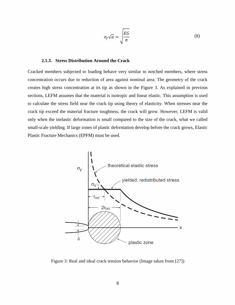
8
𝜎𝑓√𝑎 = √𝐸𝐺
𝜋 (8)
2.1.3. Stress Distribution Around the Crack
Cracked members subjected to loading behave very similar to notched members, where stress
concentration occurs due to reduction of area against nominal area. The geometry of the crack
creates high stress concentration at its tip as shown in the Figure 3. As explained in previous
sections, LEFM assumes that the material is isotropic and linear elastic. This assumption is used
to calculate the stress field near the crack tip using theory of elasticity. When stresses near the
crack tip exceed the material fracture toughness, the crack will grow. However, LEFM is valid
only when the inelastic deformation is small compared to the size of the crack, what we called
small-scale yielding. If large zones of plastic deformation develop before the crack grows, Elastic
Plastic Fracture Mechanics (EPFM) must be used.
Figure 3: Real and ideal crack tension behavior (Image taken from [27])
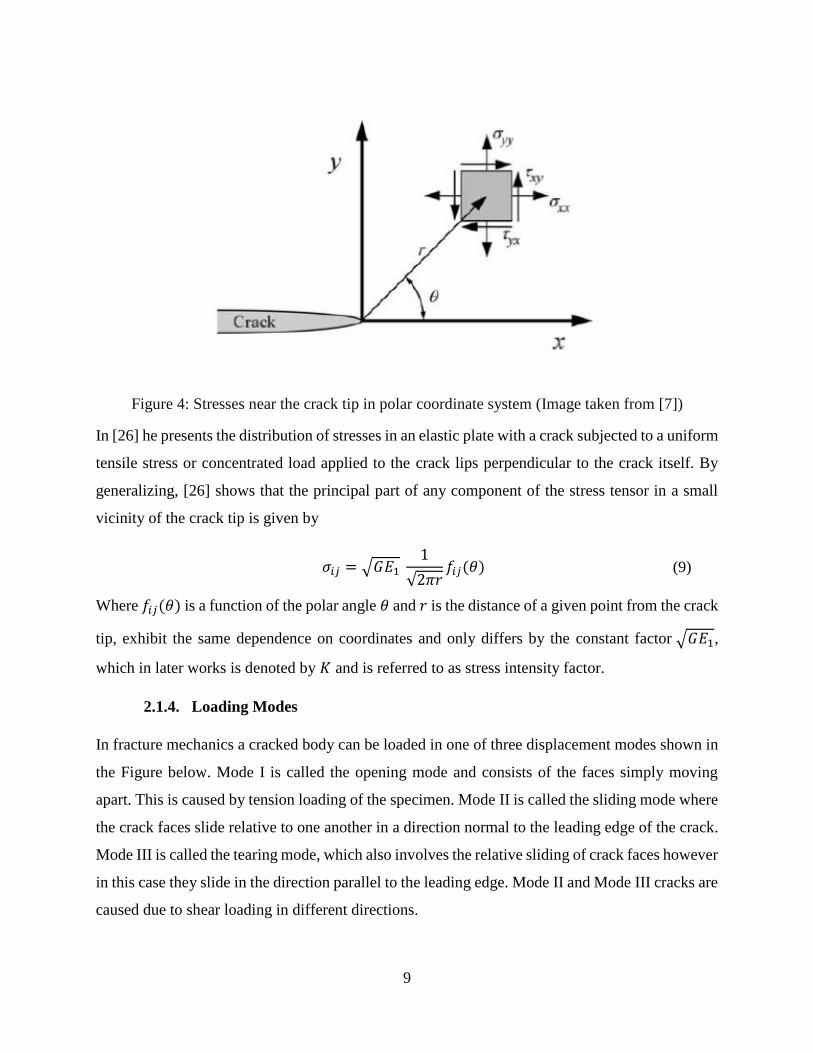
9
Figure 4: Stresses near the crack tip in polar coordinate system (Image taken from [7])
In [26] he presents the distribution of stresses in an elastic plate with a crack subjected to a uniform
tensile stress or concentrated load applied to the crack lips perpendicular to the crack itself. By
generalizing, [26] shows that the principal part of any component of the stress tensor in a small
vicinity of the crack tip is given by
𝜎𝑖𝑗 = √𝐺𝐸1 1
√2𝜋𝑟𝑓𝑖𝑗(𝜃) (9)
Where 𝑓𝑖𝑗(𝜃) is a function of the polar angle 𝜃 and 𝑟 is the distance of a given point from the crack
tip, exhibit the same dependence on coordinates and only differs by the constant factor √𝐺𝐸1,
which in later works is denoted by 𝐾 and is referred to as stress intensity factor.
2.1.4. Loading Modes
In fracture mechanics a cracked body can be loaded in one of three displacement modes shown in
the Figure below. Mode I is called the opening mode and consists of the faces simply moving
apart. This is caused by tension loading of the specimen. Mode II is called the sliding mode where
the crack faces slide relative to one another in a direction normal to the leading edge of the crack.
Mode III is called the tearing mode, which also involves the relative sliding of crack faces however
in this case they slide in the direction parallel to the leading edge. Mode II and Mode III cracks are
caused due to shear loading in different directions.
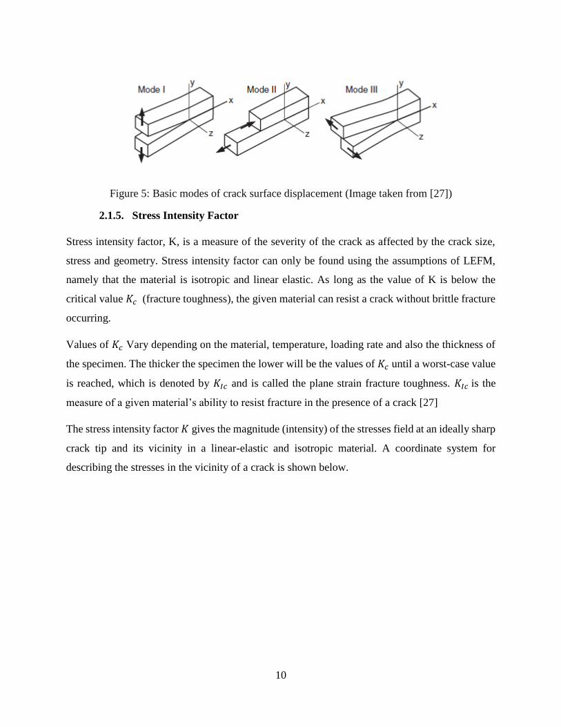
10
Figure 5: Basic modes of crack surface displacement (Image taken from [27])
2.1.5. Stress Intensity Factor
Stress intensity factor, K, is a measure of the severity of the crack as affected by the crack size,
stress and geometry. Stress intensity factor can only be found using the assumptions of LEFM,
namely that the material is isotropic and linear elastic. As long as the value of K is below the
critical value 𝐾𝑐 (fracture toughness), the given material can resist a crack without brittle fracture
occurring.
Values of 𝐾𝑐 Vary depending on the material, temperature, loading rate and also the thickness of
the specimen. The thicker the specimen the lower will be the values of 𝐾𝑐 until a worst-case value
is reached, which is denoted by 𝐾𝐼𝑐 and is called the plane strain fracture toughness. 𝐾𝐼𝑐 is the
measure of a given material’s ability to resist fracture in the presence of a crack [27]
The stress intensity factor 𝐾 gives the magnitude (intensity) of the stresses field at an ideally sharp
crack tip and its vicinity in a linear-elastic and isotropic material. A coordinate system for
describing the stresses in the vicinity of a crack is shown below.
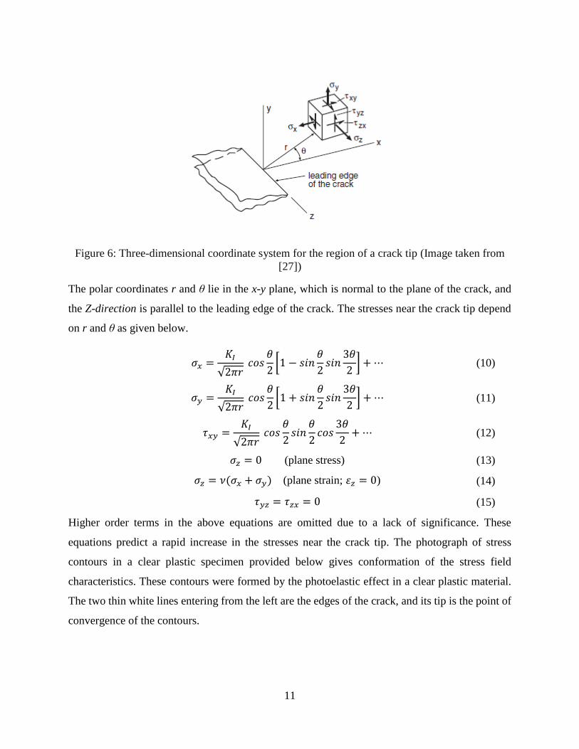
11
Figure 6: Three-dimensional coordinate system for the region of a crack tip (Image taken from
[27])
The polar coordinates r and θ lie in the x-y plane, which is normal to the plane of the crack, and
the Z-direction is parallel to the leading edge of the crack. The stresses near the crack tip depend
on r and θ as given below.
𝜎𝑥 =𝐾𝐼
√2𝜋𝑟 𝑐𝑜𝑠
𝜃
2[1 − 𝑠𝑖𝑛
𝜃
2𝑠𝑖𝑛
3𝜃
2] + ⋯ (10)
𝜎𝑦 =𝐾𝐼
√2𝜋𝑟 𝑐𝑜𝑠
𝜃
2[1 + 𝑠𝑖𝑛
𝜃
2𝑠𝑖𝑛
3𝜃
2] + ⋯ (11)
𝜏𝑥𝑦 =𝐾𝐼
√2𝜋𝑟 𝑐𝑜𝑠
𝜃
2𝑠𝑖𝑛
𝜃
2𝑐𝑜𝑠
3𝜃
2+ ⋯ (12)
𝜎𝑧 = 0 (plane stress) (13)
𝜎𝑧 = 𝜈(𝜎𝑥 + 𝜎𝑦) (plane strain; 휀𝑧 = 0) (14)
𝜏𝑦𝑧 = 𝜏𝑧𝑥 = 0 (15)
Higher order terms in the above equations are omitted due to a lack of significance. These
equations predict a rapid increase in the stresses near the crack tip. The photograph of stress
contours in a clear plastic specimen provided below gives conformation of the stress field
characteristics. These contours were formed by the photoelastic effect in a clear plastic material.
The two thin white lines entering from the left are the edges of the crack, and its tip is the point of
convergence of the contours.
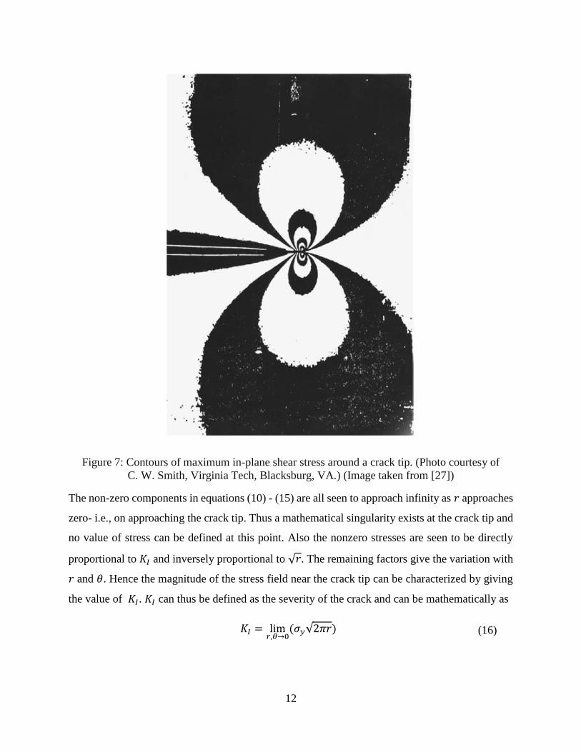
12
Figure 7: Contours of maximum in-plane shear stress around a crack tip. (Photo courtesy of
C. W. Smith, Virginia Tech, Blacksburg, VA.) (Image taken from [27])
The non-zero components in equations (10) - (15) are all seen to approach infinity as 𝑟 approaches
zero- i.e., on approaching the crack tip. Thus a mathematical singularity exists at the crack tip and
no value of stress can be defined at this point. Also the nonzero stresses are seen to be directly
proportional to 𝐾𝐼 and inversely proportional to √𝑟. The remaining factors give the variation with
𝑟 and 𝜃. Hence the magnitude of the stress field near the crack tip can be characterized by giving
the value of 𝐾𝐼. 𝐾𝐼 can thus be defined as the severity of the crack and can be mathematically as
𝐾𝐼 = lim𝑟,𝜃→0
(𝜎𝑦√2𝜋𝑟) (16)
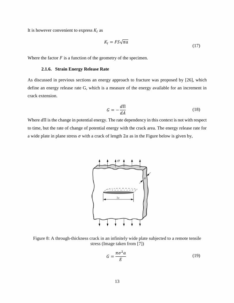
13
It is however convenient to express 𝐾𝐼 as
𝐾𝐼 = 𝐹𝑆√𝜋𝑎
(17)
Where the factor 𝐹 is a function of the geometry of the specimen.
2.1.6. Strain Energy Release Rate
As discussed in previous sections an energy approach to fracture was proposed by [26], which
define an energy release rate G, which is a measure of the energy available for an increment in
crack extension.
𝐺 = −𝑑Π
𝑑𝐴 (18)
Where 𝑑Π is the change in potential energy. The rate dependency in this context is not with respect
to time, but the rate of change of potential energy with the crack area. The energy release rate for
a wide plate in plane stress 𝜎 with a crack of length 2𝑎 as in the Figure below is given by,
Figure 8: A through-thickness crack in an infinitely wide plate subjected to a remote tensile
stress (Image taken from [7])
𝐺 =𝜋𝜎2𝑎
𝐸 (19)
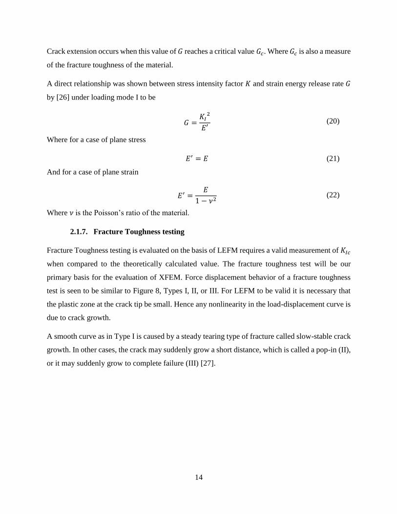
14
Crack extension occurs when this value of 𝐺 reaches a critical value 𝐺𝑐. Where 𝐺𝑐 is also a measure
of the fracture toughness of the material.
A direct relationship was shown between stress intensity factor 𝐾 and strain energy release rate 𝐺
by [26] under loading mode I to be
𝐺 =𝐾𝐼
2
𝐸′ (20)
Where for a case of plane stress
𝐸′ = 𝐸 (21)
And for a case of plane strain
𝐸′ =𝐸
1 − 𝜈2 (22)
Where 𝜈 is the Poisson’s ratio of the material.
2.1.7. Fracture Toughness testing
Fracture Toughness testing is evaluated on the basis of LEFM requires a valid measurement of 𝐾𝐼𝑐
when compared to the theoretically calculated value. The fracture toughness test will be our
primary basis for the evaluation of XFEM. Force displacement behavior of a fracture toughness
test is seen to be similar to Figure 8, Types I, II, or III. For LEFM to be valid it is necessary that
the plastic zone at the crack tip be small. Hence any nonlinearity in the load-displacement curve is
due to crack growth.
A smooth curve as in Type I is caused by a steady tearing type of fracture called slow-stable crack
growth. In other cases, the crack may suddenly grow a short distance, which is called a pop-in (II),
or it may suddenly grow to complete failure (III) [27].
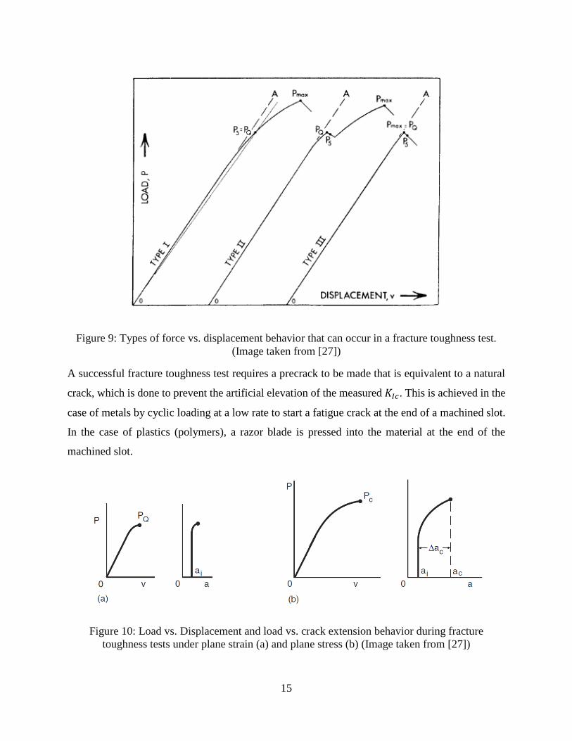
15
Figure 9: Types of force vs. displacement behavior that can occur in a fracture toughness test.
(Image taken from [27])
A successful fracture toughness test requires a precrack to be made that is equivalent to a natural
crack, which is done to prevent the artificial elevation of the measured 𝐾𝐼𝑐. This is achieved in the
case of metals by cyclic loading at a low rate to start a fatigue crack at the end of a machined slot.
In the case of plastics (polymers), a razor blade is pressed into the material at the end of the
machined slot.
Figure 10: Load vs. Displacement and load vs. crack extension behavior during fracture
toughness tests under plane strain (a) and plane stress (b) (Image taken from [27])
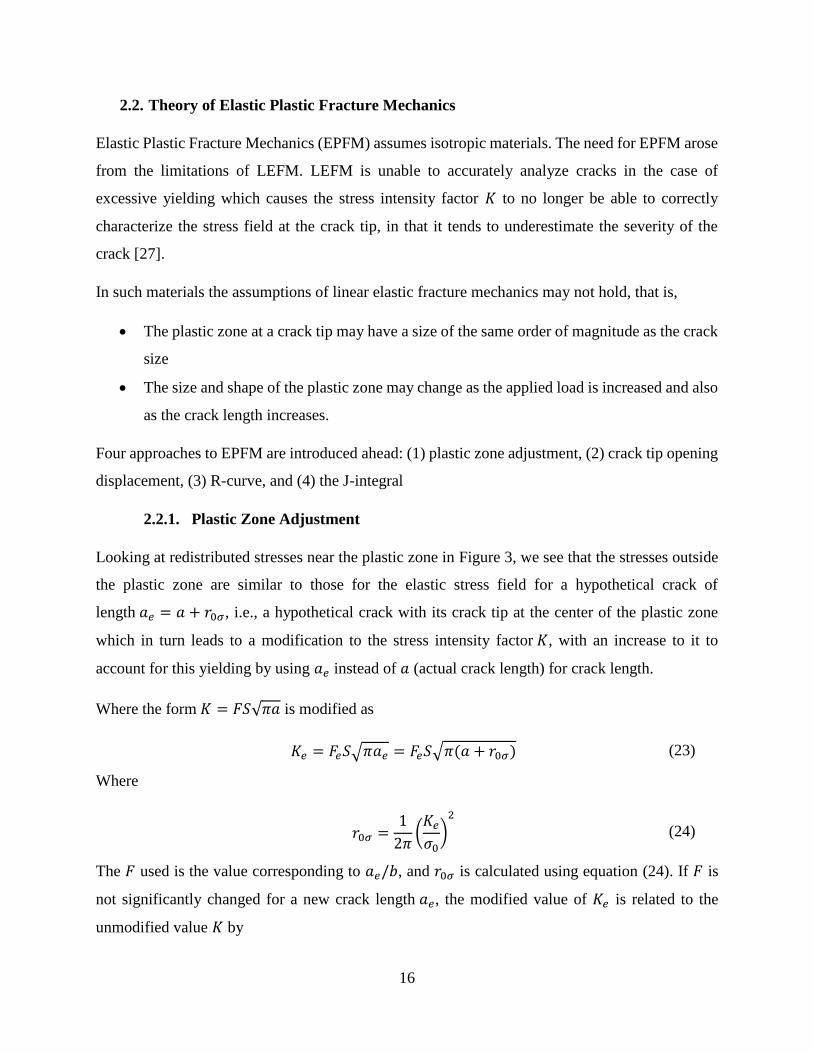
16
2.2. Theory of Elastic Plastic Fracture Mechanics
Elastic Plastic Fracture Mechanics (EPFM) assumes isotropic materials. The need for EPFM arose
from the limitations of LEFM. LEFM is unable to accurately analyze cracks in the case of
excessive yielding which causes the stress intensity factor 𝐾 to no longer be able to correctly
characterize the stress field at the crack tip, in that it tends to underestimate the severity of the
crack [27].
In such materials the assumptions of linear elastic fracture mechanics may not hold, that is,
The plastic zone at a crack tip may have a size of the same order of magnitude as the crack
size
The size and shape of the plastic zone may change as the applied load is increased and also
as the crack length increases.
Four approaches to EPFM are introduced ahead: (1) plastic zone adjustment, (2) crack tip opening
displacement, (3) R-curve, and (4) the J-integral
2.2.1. Plastic Zone Adjustment
Looking at redistributed stresses near the plastic zone in Figure 3, we see that the stresses outside
the plastic zone are similar to those for the elastic stress field for a hypothetical crack of
length 𝑎𝑒 = 𝑎 + 𝑟0𝜎, i.e., a hypothetical crack with its crack tip at the center of the plastic zone
which in turn leads to a modification to the stress intensity factor 𝐾, with an increase to it to
account for this yielding by using 𝑎𝑒 instead of 𝑎 (actual crack length) for crack length.
Where the form 𝐾 = 𝐹𝑆√𝜋𝑎 is modified as
𝐾𝑒 = 𝐹𝑒𝑆√𝜋𝑎𝑒 = 𝐹𝑒𝑆√𝜋(𝑎 + 𝑟0𝜎) (23)
Where
𝑟0𝜎 =1
2𝜋(𝐾𝑒
𝜎0)2
(24)
The 𝐹 used is the value corresponding to 𝑎𝑒/𝑏, and 𝑟0𝜎 is calculated using equation (24). If 𝐹 is
not significantly changed for a new crack length 𝑎𝑒, the modified value of 𝐾𝑒 is related to the
unmodified value 𝐾 by
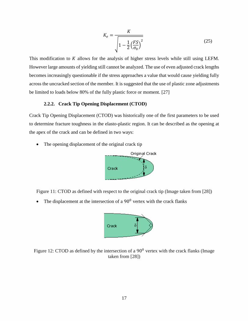
17
𝐾𝑒 =𝐾
√1 −12 (
𝐹𝑆𝜎0
)2
(25)
This modification to 𝐾 allows for the analysis of higher stress levels while still using LEFM.
However large amounts of yielding still cannot be analyzed. The use of even adjusted crack lengths
becomes increasingly questionable if the stress approaches a value that would cause yielding fully
across the uncracked section of the member. It is suggested that the use of plastic zone adjustments
be limited to loads below 80% of the fully plastic force or moment. [27]
2.2.2. Crack Tip Opening Displacement (CTOD)
Crack Tip Opening Displacement (CTOD) was historically one of the first parameters to be used
to determine fracture toughness in the elasto-plastic region. It can be described as the opening at
the apex of the crack and can be defined in two ways:
The opening displacement of the original crack tip
Figure 11: CTOD as defined with respect to the original crack tip (Image taken from [28])
The displacement at the intersection of a 900 vertex with the crack flanks
Figure 12: CTOD as defined by the intersection of a 900 vertex with the crack flanks (Image
taken from [28])
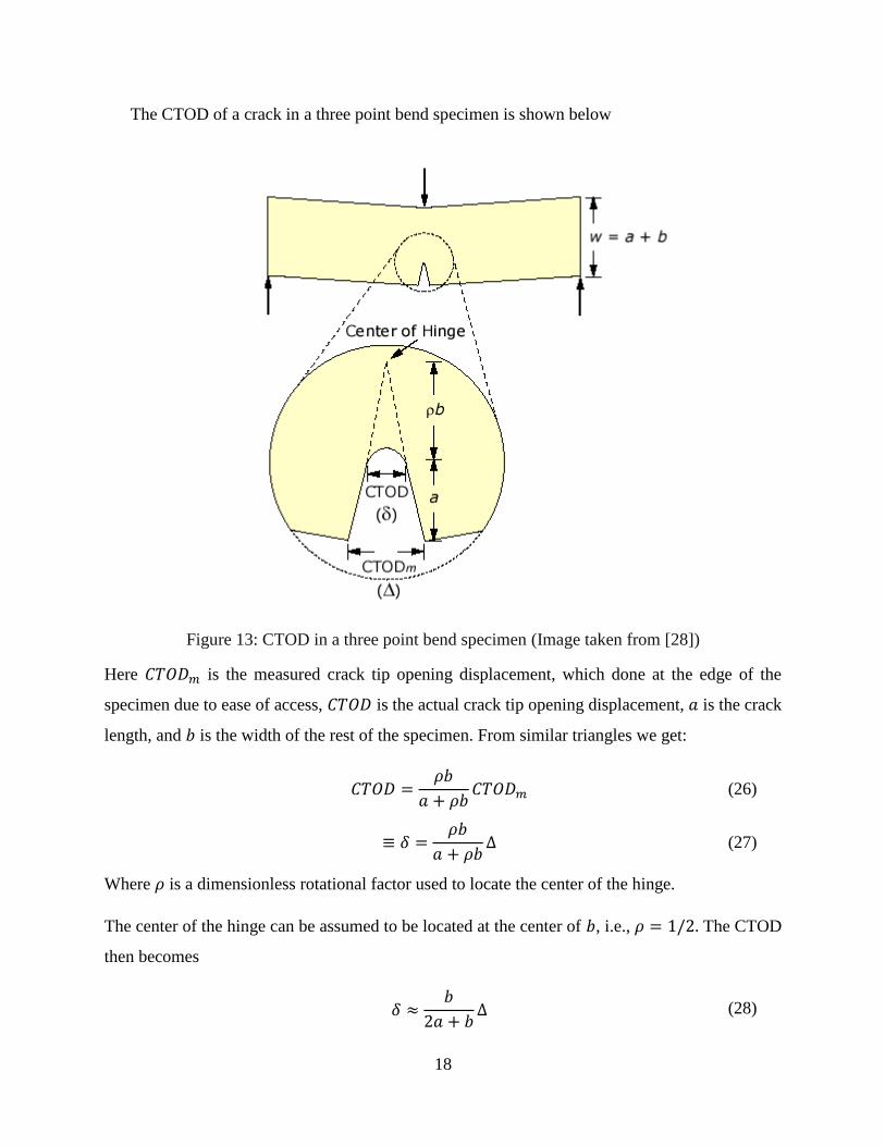
18
The CTOD of a crack in a three point bend specimen is shown below
Figure 13: CTOD in a three point bend specimen (Image taken from [28])
Here 𝐶𝑇𝑂𝐷𝑚 is the measured crack tip opening displacement, which done at the edge of the
specimen due to ease of access, 𝐶𝑇𝑂𝐷 is the actual crack tip opening displacement, 𝑎 is the crack
length, and 𝑏 is the width of the rest of the specimen. From similar triangles we get:
𝐶𝑇𝑂𝐷 =𝜌𝑏
𝑎 + 𝜌𝑏𝐶𝑇𝑂𝐷𝑚 (26)
≡ 𝛿 =𝜌𝑏
𝑎 + 𝜌𝑏∆ (27)
Where 𝜌 is a dimensionless rotational factor used to locate the center of the hinge.
The center of the hinge can be assumed to be located at the center of 𝑏, i.e., 𝜌 = 1/2. The CTOD
then becomes
𝛿 ≈𝑏
2𝑎 + 𝑏∆ (28)
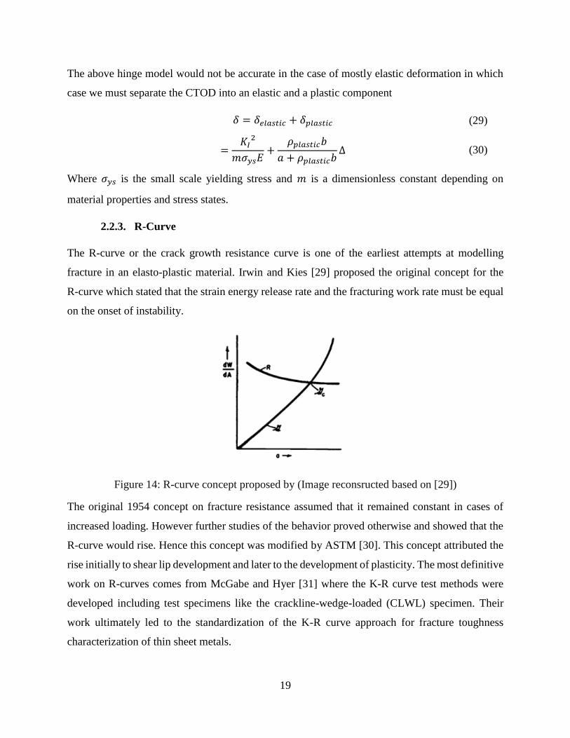
19
The above hinge model would not be accurate in the case of mostly elastic deformation in which
case we must separate the CTOD into an elastic and a plastic component
𝛿 = 𝛿𝑒𝑙𝑎𝑠𝑡𝑖𝑐 + 𝛿𝑝𝑙𝑎𝑠𝑡𝑖𝑐 (29)
=𝐾𝐼
2
𝑚𝜎𝑦𝑠𝐸+
𝜌𝑝𝑙𝑎𝑠𝑡𝑖𝑐𝑏
𝑎 + 𝜌𝑝𝑙𝑎𝑠𝑡𝑖𝑐𝑏∆ (30)
Where 𝜎𝑦𝑠 is the small scale yielding stress and 𝑚 is a dimensionless constant depending on
material properties and stress states.
2.2.3. R-Curve
The R-curve or the crack growth resistance curve is one of the earliest attempts at modelling
fracture in an elasto-plastic material. Irwin and Kies [29] proposed the original concept for the
R-curve which stated that the strain energy release rate and the fracturing work rate must be equal
on the onset of instability.
Figure 14: R-curve concept proposed by (Image reconsructed based on [29])
The original 1954 concept on fracture resistance assumed that it remained constant in cases of
increased loading. However further studies of the behavior proved otherwise and showed that the
R-curve would rise. Hence this concept was modified by ASTM [30]. This concept attributed the
rise initially to shear lip development and later to the development of plasticity. The most definitive
work on R-curves comes from McGabe and Hyer [31] where the K-R curve test methods were
developed including test specimens like the crackline-wedge-loaded (CLWL) specimen. Their
work ultimately led to the standardization of the K-R curve approach for fracture toughness
characterization of thin sheet metals.
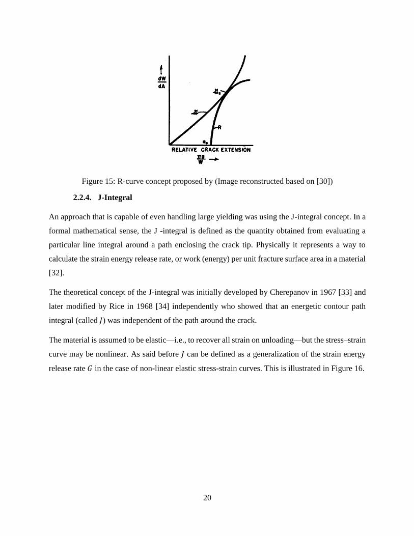
20
Figure 15: R-curve concept proposed by (Image reconstructed based on [30])
2.2.4. J-Integral
An approach that is capable of even handling large yielding was using the J-integral concept. In a
formal mathematical sense, the J -integral is defined as the quantity obtained from evaluating a
particular line integral around a path enclosing the crack tip. Physically it represents a way to
calculate the strain energy release rate, or work (energy) per unit fracture surface area in a material
[32].
The theoretical concept of the J-integral was initially developed by Cherepanov in 1967 [33] and
later modified by Rice in 1968 [34] independently who showed that an energetic contour path
integral (called 𝐽) was independent of the path around the crack.
The material is assumed to be elastic—i.e., to recover all strain on unloading—but the stress–strain
curve may be nonlinear. As said before 𝐽 can be defined as a generalization of the strain energy
release rate 𝐺 in the case of non-linear elastic stress-strain curves. This is illustrated in Figure 16.
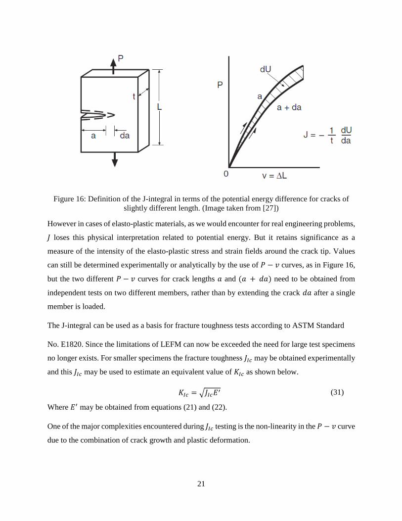
21
Figure 16: Definition of the J-integral in terms of the potential energy difference for cracks of
slightly different length. (Image taken from [27])
However in cases of elasto-plastic materials, as we would encounter for real engineering problems,
𝐽 loses this physical interpretation related to potential energy. But it retains significance as a
measure of the intensity of the elasto-plastic stress and strain fields around the crack tip. Values
can still be determined experimentally or analytically by the use of 𝑃 − 𝑣 curves, as in Figure 16,
but the two different 𝑃 − 𝑣 curves for crack lengths 𝑎 and (𝑎 + 𝑑𝑎) need to be obtained from
independent tests on two different members, rather than by extending the crack 𝑑𝑎 after a single
member is loaded.
The J-integral can be used as a basis for fracture toughness tests according to ASTM Standard
No. E1820. Since the limitations of LEFM can now be exceeded the need for large test specimens
no longer exists. For smaller specimens the fracture toughness 𝐽𝐼𝑐 may be obtained experimentally
and this 𝐽𝐼𝑐 may be used to estimate an equivalent value of 𝐾𝐼𝑐 as shown below.
𝐾𝐼𝑐 = √𝐽𝐼𝑐𝐸′ (31)
Where 𝐸′ may be obtained from equations (21) and (22).
One of the major complexities encountered during 𝐽𝐼𝑐 testing is the non-linearity in the 𝑃 − 𝑣 curve
due to the combination of crack growth and plastic deformation.
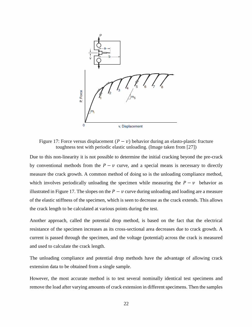
22
Figure 17: Force versus displacement (𝑃 − 𝑣) behavior during an elasto-plastic fracture
toughness test with periodic elastic unloading. (Image taken from [27])
Due to this non-linearity it is not possible to determine the initial cracking beyond the pre-crack
by conventional methods from the 𝑃 − 𝑣 curve, and a special means is necessary to directly
measure the crack growth. A common method of doing so is the unloading compliance method,
which involves periodically unloading the specimen while measuring the 𝑃 − 𝑣 behavior as
illustrated in Figure 17. The slopes on the 𝑃 − 𝑣 curve during unloading and loading are a measure
of the elastic stiffness of the specimen, which is seen to decrease as the crack extends. This allows
the crack length to be calculated at various points during the test.
Another approach, called the potential drop method, is based on the fact that the electrical
resistance of the specimen increases as its cross-sectional area decreases due to crack growth. A
current is passed through the specimen, and the voltage (potential) across the crack is measured
and used to calculate the crack length.
The unloading compliance and potential drop methods have the advantage of allowing crack
extension data to be obtained from a single sample.
However, the most accurate method is to test several nominally identical test specimens and
remove the load after varying amounts of crack extension in different specimens. Then the samples
23
are heated to tint (slightly oxidize) the fresh fracture surface so that it is easily observed, next they
are broken into two pieces, and finally the amounts of crack growth are measured through a
microscope.
2.3. The Finite Element Method (FEM)
The Finite Element Method (FEM) is a numerical method used to solve problems described by
partial differential equations or can be formulated as functional minimization. FEM is also known
as Finite Element Analysis (FEA). In FEM the domain of the problem is represented as an
assembly of finite elements. Approximating functions in finite elements are determined in terms
of nodal values of the physical fields which need to be calculated. Here a continuous problem is
discretized into finite elements and then solved for the unknown nodal values. In case of a linear
problem a system of linear equations need to be solved to obtain the nodal values. These nodal
values can be used to recover the values within the finite element itself.
Two main features of FEM that are worth mentioning:
The usage of simple approximation functions to determine nodal values can yield results
of higher accuracy by simply increasing the number of elements.
Locality of approximation leads to a set of sparse equation systems for a discretized
problems which allows us to solve problems with a very large number of nodal unknowns.
2.3.1. Methodology of FEM
Solving a finite element problem is briefly described in the following steps.
Discretize the continuum: Initially the solution region of the problem is divided into finite
elements. The finite element mesh can be generated by a preprocessor program or be
defined by the user manually. The mesh can be described as a set of several arrays/matrices
which have nodal coordinates and element connectivity.
Select interpolation functions: An interpolation function is used to interpolate the field
variable, such as displacement, over the element. Polynomials are commonly used as
interpolation functions. The degree of the polynomial is defined by the number of nodes
associated with a particular element.
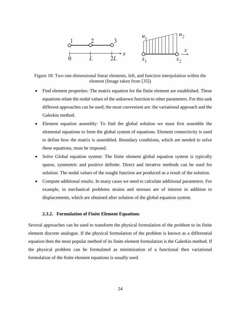
24
Figure 18: Two one-dimensional linear elements, left, and function interpolation within the
element (Image taken from [35])
Find element properties: The matrix equation for the finite element are established. These
equations relate the nodal values of the unknown function to other parameters. For this task
different approaches can be used; the most convenient are: the variational approach and the
Galerkin method.
Element equation assembly: To find the global solution we must first assemble the
elemental equations to form the global system of equations. Element connectivity is used
to define how the matrix is assembled. Boundary conditions, which are needed to solve
these equations, must be imposed.
Solve Global equation system: The finite element global equation system is typically
sparse, symmetric and positive definite. Direct and iterative methods can be used for
solution. The nodal values of the sought function are produced as a result of the solution.
Compute additional results. In many cases we need to calculate additional parameters. For
example, in mechanical problems strains and stresses are of interest in addition to
displacements, which are obtained after solution of the global equation system.
2.3.2. Formulation of Finite Element Equations
Several approaches can be used to transform the physical formulation of the problem to its finite
element discrete analogue. If the physical formulation of the problem is known as a differential
equation then the most popular method of its finite element formulation is the Galerkin method. If
the physical problem can be formulated as minimization of a functional then variational
formulation of the finite element equations is usually used.
25
2.3.2.1. Galerkin Method
In mathematics, in the area of numerical analysis, Galerkin methods are a class of methods for
converting a continuous operator problem (such as a differential equation) to a discrete problem.
In principle, it is the equivalent of applying the method of variation of parameters to a function
space, by converting the equation to a weak formulation. Typically one then applies some
constraints on the function space to characterize the space with a finite set of basis functions.
Galerkin's method provides powerful numerical solution to differential equations and modal
analysis [36].
The Galerkin method of weighted residuals, is used to calculate the global stiffness matrix in the
finite element method [37].
Consider a simple one-dimensional example [35], to numerically solve the following differential
equation:
𝑎𝑑2𝑢
𝑑𝑥2+ 𝑏 = 0, 0 ≤ 𝑥 ≤ 2𝐿 (32)
With the boundary conditions
𝑢|𝑥=0 = 0
𝑎𝑑𝑢
𝑑𝑥|𝑥=2𝐿 = 𝑅
(33)
Here 𝑢 is an unknown solution. This problem will be solved using two linear one-dimensional
finite elements as shown in Figure 18.
Consider the finite element shown on the right of the Figure. The element has two nodes and the
function 𝑢(𝑥) can be approximated as shown below
𝑢 = 𝑁1𝑢1 + 𝑁2𝑢2 = [𝑁]{𝑢} (34)
Where
[𝑁] = [𝑁1 𝑁2] (35)
26
{𝑢} = {𝑢1 𝑢2}
𝑁𝑖 are also called shape functions.
𝑁1 = 1 −𝑥 − 𝑥1
𝑥2 − 𝑥1
𝑁2 =𝑥 − 𝑥1
𝑥2 − 𝑥1
(36)
These shape functions are used to interpolate 𝑢(𝑥) using its nodal values. The nodal values 𝑢1
and 𝑢2 are unknown and are to be determined from the discrete global system of equations.
After substituting 𝑢 expressed through its nodal values and shape functions, in the differential
equation, it has the following approximate form:
𝑎𝑑2
𝑑𝑥2[𝑁]{𝑢} + 𝑏 = 𝜓 (37)
Where 𝜓 is a non-zero residual due to the approximate representation of a function within the finite
element. This residual is minimized multiplying equation 37 by the shape function and integrating
it over the length of the element and equating it to zero. Doing this we get
∫ [𝑁]𝑇𝑎𝑑2
𝑑𝑥2[𝑁]{𝑢}𝑑𝑥
𝑥2
𝑥1
+ ∫ [𝑁]𝑇𝑏𝑑𝑥𝑥2
𝑥1
= 0 (38)
Integrating by parts we get a discrete form of the differential equation for the finite element.
∫ [𝑑𝑁
𝑑𝑥]𝑇
𝑎 [𝑑𝑁
𝑑𝑥] 𝑑𝑥
𝑥2
𝑥1
{𝑢} − ∫ [𝑁]𝑇𝑏𝑑𝑥 − {01}
𝑥2
𝑥1
𝑎𝑑𝑢
𝑑𝑥|𝑥=𝑥2
+ {10} 𝑎
𝑑𝑢
𝑑𝑥|𝑥=𝑥1
= 0
(39)
Such a relation for a finite element is represented as
[𝑘]{𝑢} = {𝑓}
[𝑘] = ∫ [𝑑𝑁
𝑑𝑥]𝑇
𝑎 [𝑑𝑁
𝑑𝑥] 𝑑𝑥
𝑥2
𝑥1
{𝑓} = ∫ [𝑁]𝑇𝑏𝑑𝑥 + {01}
𝑥2
𝑥1
𝑎𝑑𝑢
𝑑𝑥|𝑥=𝑥2
− {10} 𝑎
𝑑𝑢
𝑑𝑥|𝑥=𝑥1
(40)
In solid mechanics [𝑘] is referred to as the stiffness matrix and {𝑓} is referred to as the load vector.
2.3.2.2. Variational Formulation
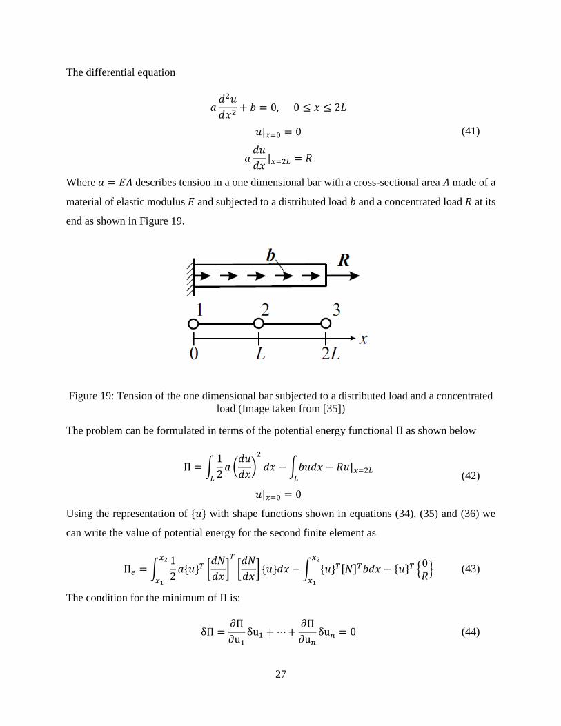
27
The differential equation
𝑎𝑑2𝑢
𝑑𝑥2+ 𝑏 = 0, 0 ≤ 𝑥 ≤ 2𝐿
𝑢|𝑥=0 = 0
𝑎𝑑𝑢
𝑑𝑥|𝑥=2𝐿 = 𝑅
(41)
Where 𝑎 = 𝐸𝐴 describes tension in a one dimensional bar with a cross-sectional area 𝐴 made of a
material of elastic modulus 𝐸 and subjected to a distributed load 𝑏 and a concentrated load 𝑅 at its
end as shown in Figure 19.
Figure 19: Tension of the one dimensional bar subjected to a distributed load and a concentrated
load (Image taken from [35])
The problem can be formulated in terms of the potential energy functional Π as shown below
Π = ∫
1
2𝑎 (
𝑑𝑢
𝑑𝑥)2
𝑑𝑥 − ∫𝑏𝑢𝑑𝑥 − 𝑅𝑢|𝑥=2𝐿𝐿𝐿
𝑢|𝑥=0 = 0
(42)
Using the representation of {𝑢} with shape functions shown in equations (34), (35) and (36) we
can write the value of potential energy for the second finite element as
Π𝑒 = ∫1
2𝑎{𝑢}𝑇 [
𝑑𝑁
𝑑𝑥]𝑇
[𝑑𝑁
𝑑𝑥] {𝑢}𝑑𝑥 − ∫ {𝑢}𝑇[𝑁]𝑇𝑏𝑑𝑥 − {𝑢}𝑇 {
0𝑅}
𝑥2
𝑥1
𝑥2
𝑥1
(43)
The condition for the minimum of Π is:
δΠ =∂Π
∂u1δu1 + ⋯+
∂Π
∂u𝑛δu𝑛 = 0 (44)
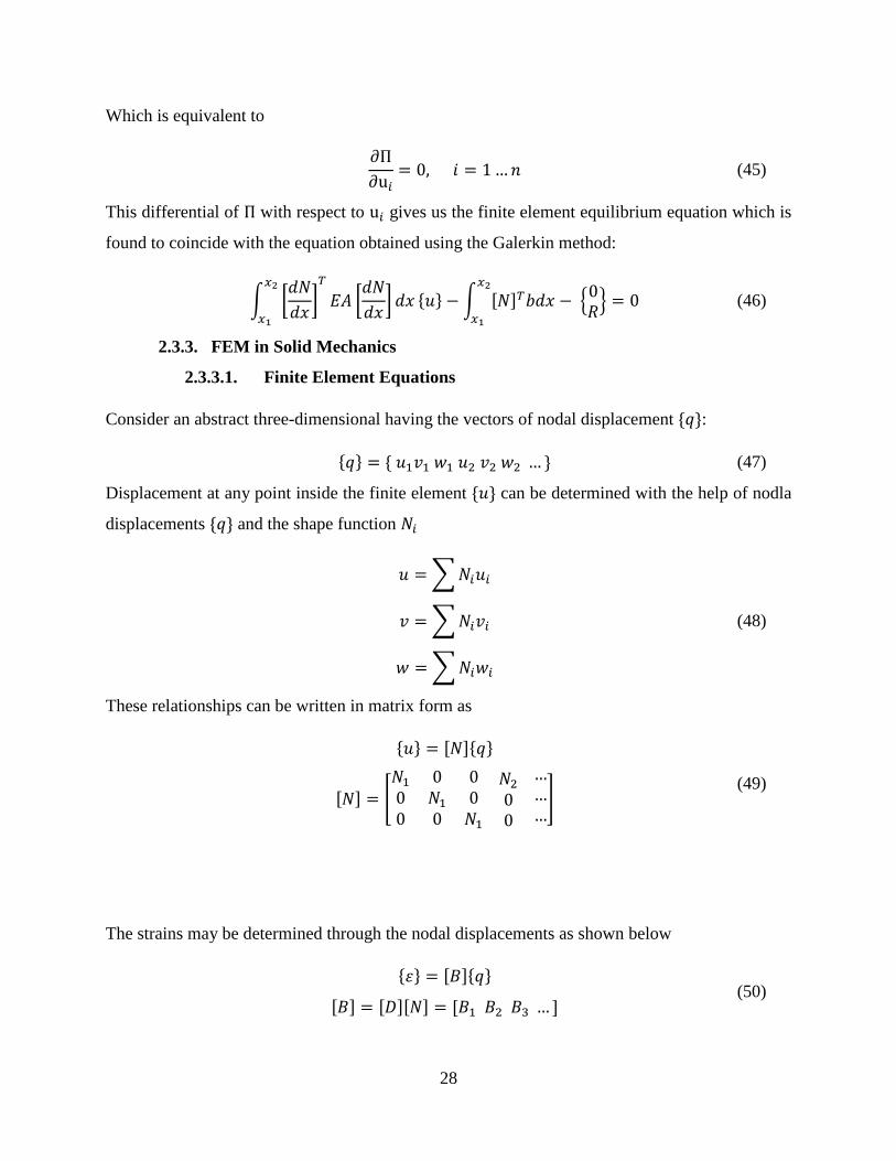
28
Which is equivalent to
∂Π
∂u𝑖= 0, 𝑖 = 1…𝑛 (45)
This differential of Π with respect to u𝑖 gives us the finite element equilibrium equation which is
found to coincide with the equation obtained using the Galerkin method:
∫ [𝑑𝑁
𝑑𝑥]𝑇
𝐸𝐴 [𝑑𝑁
𝑑𝑥] 𝑑𝑥
𝑥2
𝑥1
{𝑢} − ∫ [𝑁]𝑇𝑏𝑑𝑥 − {0𝑅}
𝑥2
𝑥1
= 0 (46)
2.3.3. FEM in Solid Mechanics
2.3.3.1. Finite Element Equations
Consider an abstract three-dimensional having the vectors of nodal displacement {𝑞}:
{𝑞} = { 𝑢1𝑣1 𝑤1 𝑢2 𝑣2 𝑤2 … } (47)
Displacement at any point inside the finite element {𝑢} can be determined with the help of nodla
displacements {𝑞} and the shape function 𝑁𝑖
𝑢 = ∑𝑁𝑖𝑢𝑖
𝑣 = ∑𝑁𝑖𝑣𝑖
𝑤 = ∑𝑁𝑖𝑤𝑖
(48)
These relationships can be written in matrix form as
{𝑢} = [𝑁]{𝑞}
[𝑁] = [
𝑁1 0 00 𝑁1 00 0 𝑁1
𝑁2
00
………
] (49)
The strains may be determined through the nodal displacements as shown below
{휀} = [𝐵]{𝑞}
[𝐵] = [𝐷][𝑁] = [𝐵1 𝐵2 𝐵3 … ] (50)
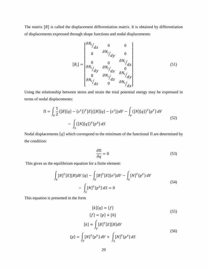
29
The matrix [𝐵] is called the displacement differentiation matrix. It is obtained by differentiation
of displacements expressed through shape functions and nodal displacements:
[𝐵𝑖] =
[ 𝜕𝑁𝑖
𝑑𝑥⁄ 0 0
0𝜕𝑁𝑖
𝑑𝑦⁄ 0
0𝜕𝑁𝑖
𝑑𝑦⁄
0𝜕𝑁𝑖
𝑑𝑧⁄
0𝜕𝑁𝑖
𝑑𝑥⁄
𝜕𝑁𝑖𝑑𝑧
⁄
0
𝜕𝑁𝑖𝑑𝑧
⁄
0𝜕𝑁𝑖
𝑑𝑦⁄
𝜕𝑁𝑖𝑑𝑥
⁄ ]
(51)
Using the relationship between stress and strain the total potential energy may be expressed in
terms of nodal displacements:
Π = ∫1
2([𝐵]{𝑞} − {휀𝑡})𝑇[𝐸]([𝐵]{𝑞} − {휀𝑡})𝑑𝑉
𝑉
− ∫([𝑁]{𝑞})𝑇{𝑝𝑉}𝑉
𝑑𝑉
− ∫([𝑁]{𝑞})𝑇{𝑝𝑆}𝑆
𝑑𝑆
(52)
Nodal displacements {𝑞} which correspond to the minimum of the functional Π are determined by
the condition:
∂Π
∂𝑞= 0 (53)
This gives us the equilibrium equation for a finite element:
∫[𝐵]𝑇[𝐸][𝐵]𝑑𝑉𝑉
{𝑞} − ∫[𝐵]𝑇[𝐸]{𝑒𝑡}𝑑𝑉𝑉
− ∫[𝑁]𝑇{𝑝𝑉}𝑉
𝑑𝑉
− ∫[𝑁]𝑇{𝑝𝑆}𝑆
𝑑𝑆 = 0
(54)
This equation is presented in the form
[𝑘]{𝑞} = {𝑓}
{𝑓} = {𝑝} + {ℎ} (55)
[𝑘] = ∫[𝐵]𝑇[𝐸][𝐵]𝑑𝑉𝑉
{𝑝} = ∫[𝑁]𝑇{𝑝𝑉}𝑉
𝑑𝑉 + ∫[𝑁]𝑇{𝑝𝑆}𝑆
𝑑𝑆
(56)
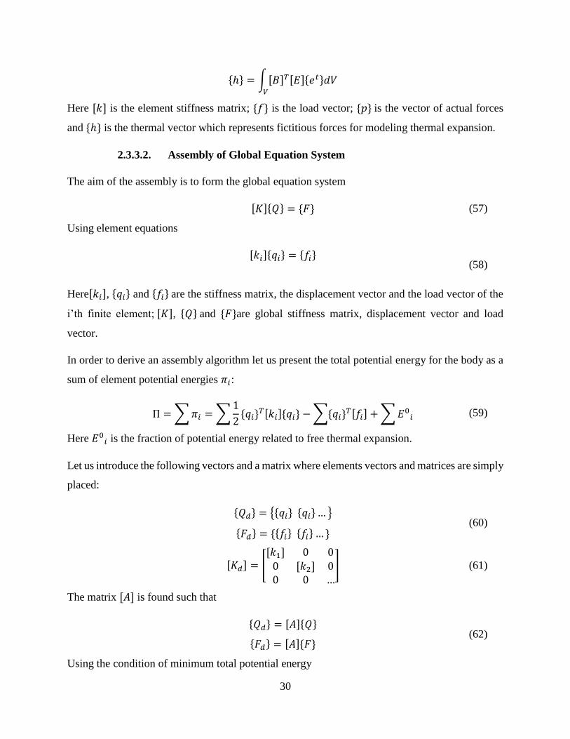
30
{ℎ} = ∫[𝐵]𝑇[𝐸]{𝑒𝑡}𝑑𝑉𝑉
Here [𝑘] is the element stiffness matrix; {𝑓} is the load vector; {𝑝} is the vector of actual forces
and {ℎ} is the thermal vector which represents fictitious forces for modeling thermal expansion.
2.3.3.2. Assembly of Global Equation System
The aim of the assembly is to form the global equation system
[𝐾]{𝑄} = {𝐹} (57)
Using element equations
[𝑘𝑖]{𝑞𝑖} = {𝑓𝑖}
(58)
Here[𝑘𝑖], {𝑞𝑖} and {𝑓𝑖} are the stiffness matrix, the displacement vector and the load vector of the
i’th finite element; [𝐾], {𝑄} and {𝐹}are global stiffness matrix, displacement vector and load
vector.
In order to derive an assembly algorithm let us present the total potential energy for the body as a
sum of element potential energies 𝜋𝑖:
Π = ∑𝜋𝑖 = ∑1
2{𝑞𝑖}
𝑇[𝑘𝑖]{𝑞𝑖} − ∑{𝑞𝑖}𝑇[𝑓𝑖] + ∑𝐸0
𝑖 (59)
Here 𝐸0𝑖 is the fraction of potential energy related to free thermal expansion.
Let us introduce the following vectors and a matrix where elements vectors and matrices are simply
placed:
{𝑄𝑑} = {{𝑞𝑖} {𝑞𝑖}… }
{𝐹𝑑} = {{𝑓𝑖} {𝑓𝑖} … } (60)
[𝐾𝑑] = [[𝑘1] 0 00 [𝑘2] 00 0 …
] (61)
The matrix [𝐴] is found such that
{𝑄𝑑} = [𝐴]{𝑄}
{𝐹𝑑} = [𝐴]{𝐹} (62)
Using the condition of minimum total potential energy
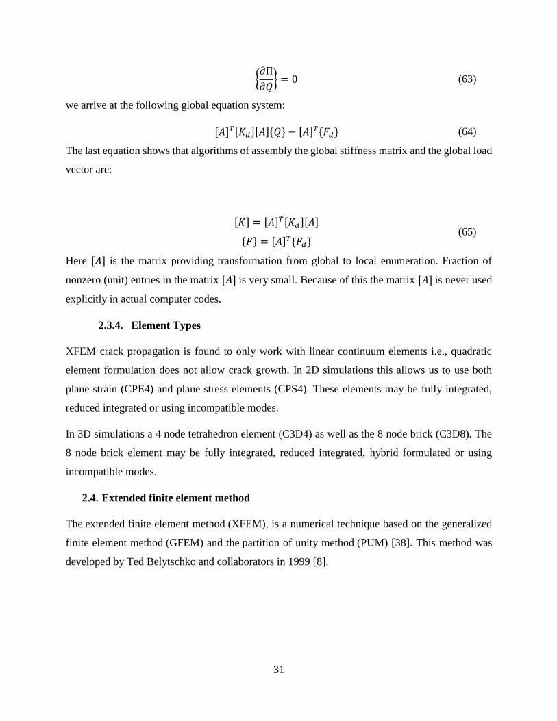
31
{∂Π
∂𝑄} = 0 (63)
we arrive at the following global equation system:
[𝐴]𝑇[𝐾𝑑][𝐴]{𝑄} − [𝐴]𝑇{𝐹𝑑} (64)
The last equation shows that algorithms of assembly the global stiffness matrix and the global load
vector are:
[𝐾] = [𝐴]𝑇[𝐾𝑑][𝐴]
{𝐹} = [𝐴]𝑇{𝐹𝑑} (65)
Here [𝐴] is the matrix providing transformation from global to local enumeration. Fraction of
nonzero (unit) entries in the matrix [𝐴] is very small. Because of this the matrix [𝐴] is never used
explicitly in actual computer codes.
2.3.4. Element Types
XFEM crack propagation is found to only work with linear continuum elements i.e., quadratic
element formulation does not allow crack growth. In 2D simulations this allows us to use both
plane strain (CPE4) and plane stress elements (CPS4). These elements may be fully integrated,
reduced integrated or using incompatible modes.
In 3D simulations a 4 node tetrahedron element (C3D4) as well as the 8 node brick (C3D8). The
8 node brick element may be fully integrated, reduced integrated, hybrid formulated or using
incompatible modes.
2.4. Extended finite element method
The extended finite element method (XFEM), is a numerical technique based on the generalized
finite element method (GFEM) and the partition of unity method (PUM) [38]. This method was
developed by Ted Belytschko and collaborators in 1999 [8].
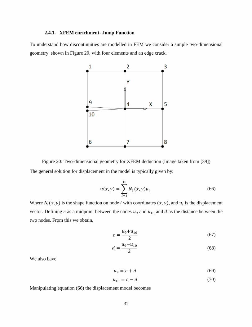
32
2.4.1. XFEM enrichment- Jump Function
To understand how discontinuities are modelled in FEM we consider a simple two-dimensional
geometry, shown in Figure 20, with four elements and an edge crack.
Figure 20: Two-dimensional geometry for XFEM deduction (Image taken from [39])
The general solution for displacement in the model is typically given by:
𝑢(𝑥, 𝑦) = ∑𝑁𝑖
10
𝑖=1
(𝑥, 𝑦)𝑢𝑖 (66)
Where 𝑁𝑖(𝑥, 𝑦) is the shape function on node 𝑖 with coordinates (𝑥, 𝑦), and 𝑢𝑖 is the displacement
vector. Defining 𝑐 as a midpoint between the nodes 𝑢9 and 𝑢10 and 𝑑 as the distance between the
two nodes. From this we obtain,
𝑐 =𝑢9+𝑢10
2 (67)
𝑑 =𝑢9−𝑢10
2 (68)
We also have
𝑢9 = 𝑐 + 𝑑 (69)
𝑢10 = 𝑐 − 𝑑 (70)
Manipulating equation (66) the displacement model becomes
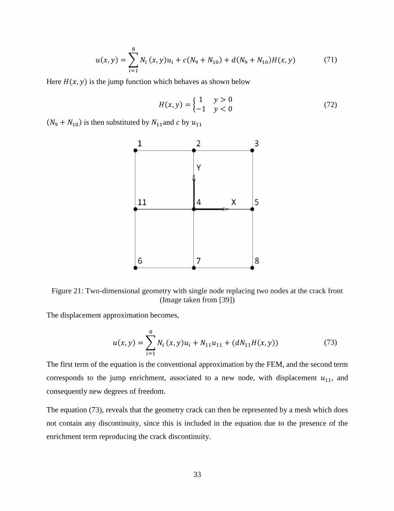
33
𝑢(𝑥, 𝑦) = ∑𝑁𝑖
8
𝑖=1
(𝑥, 𝑦)𝑢𝑖 + 𝑐(𝑁9 + 𝑁10) + 𝑑(𝑁9 + 𝑁10)𝐻(𝑥, 𝑦) (71)
Here 𝐻(𝑥, 𝑦) is the jump function which behaves as shown below
𝐻(𝑥, 𝑦) = {1 𝑦 > 0
−1 𝑦 < 0 (72)
(𝑁9 + 𝑁10) is then substituted by 𝑁11and 𝑐 by 𝑢11
Figure 21: Two-dimensional geometry with single node replacing two nodes at the crack front
(Image taken from [39])
The displacement approximation becomes,
𝑢(𝑥, 𝑦) = ∑𝑁𝑖
8
𝑖=1
(𝑥, 𝑦)𝑢𝑖 + 𝑁11𝑢11 + (𝑑𝑁11𝐻(𝑥, 𝑦)) (73)
The first term of the equation is the conventional approximation by the FEM, and the second term
corresponds to the jump enrichment, associated to a new node, with displacement 𝑢11, and
consequently new degrees of freedom.
The equation (73), reveals that the geometry crack can then be represented by a mesh which does
not contain any discontinuity, since this is included in the equation due to the presence of the
enrichment term reproducing the crack discontinuity.
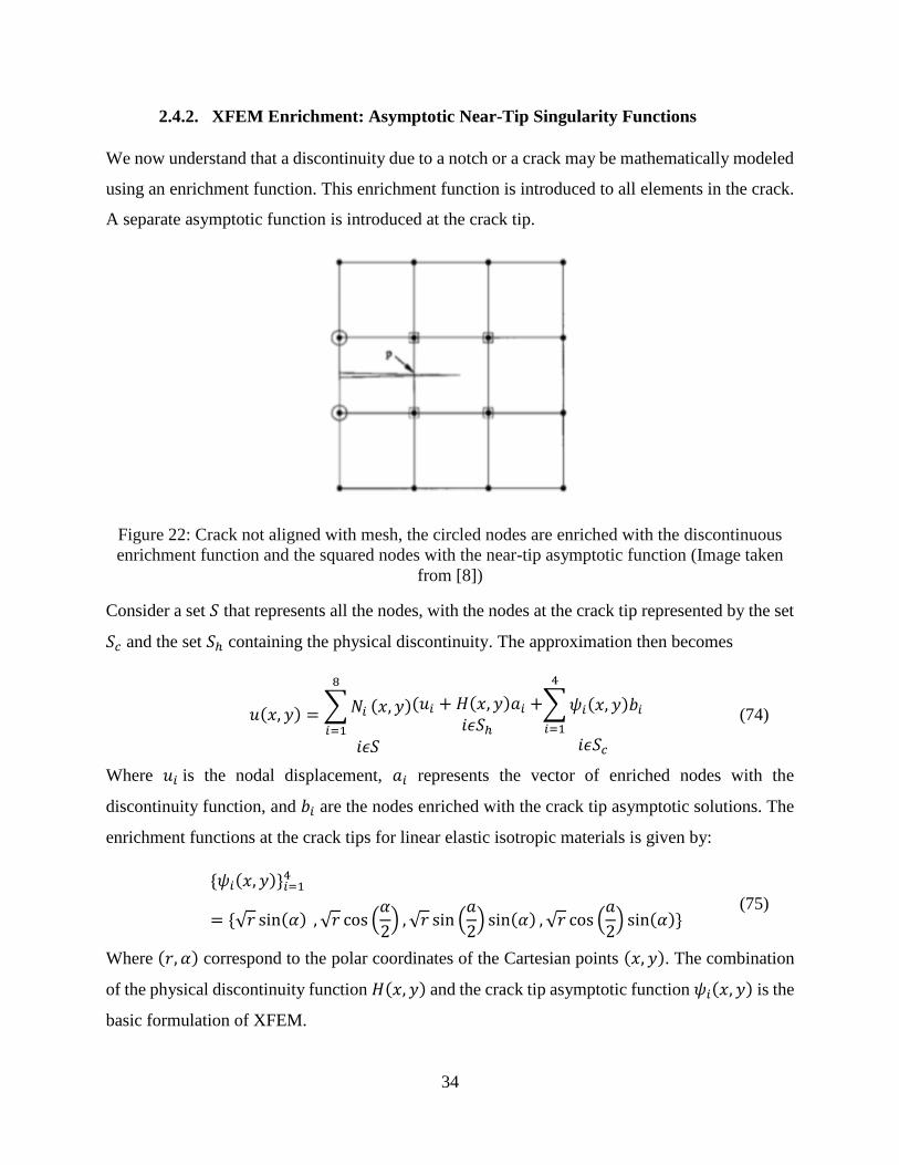
34
2.4.2. XFEM Enrichment: Asymptotic Near-Tip Singularity Functions
We now understand that a discontinuity due to a notch or a crack may be mathematically modeled
using an enrichment function. This enrichment function is introduced to all elements in the crack.
A separate asymptotic function is introduced at the crack tip.
Figure 22: Crack not aligned with mesh, the circled nodes are enriched with the discontinuous
enrichment function and the squared nodes with the near-tip asymptotic function (Image taken
from [8])
Consider a set 𝑆 that represents all the nodes, with the nodes at the crack tip represented by the set
𝑆𝑐 and the set 𝑆ℎ containing the physical discontinuity. The approximation then becomes
𝑢(𝑥, 𝑦) = ∑𝑁𝑖
8
𝑖=1
(𝑥, 𝑦)
𝑖𝜖𝑆
(𝑢𝑖 + 𝐻(𝑥, 𝑦)𝑎𝑖 +𝑖𝜖𝑆ℎ
∑𝜓𝑖(𝑥, 𝑦)𝑏𝑖
4
𝑖=1
𝑖𝜖𝑆𝑐
(74)
Where 𝑢𝑖 is the nodal displacement, 𝑎𝑖 represents the vector of enriched nodes with the
discontinuity function, and 𝑏𝑖 are the nodes enriched with the crack tip asymptotic solutions. The
enrichment functions at the crack tips for linear elastic isotropic materials is given by:
{𝜓𝑖(𝑥, 𝑦)}𝑖=14
= {√𝑟 sin(𝛼) , √𝑟 cos (𝛼
2) , √𝑟 sin (
𝑎
2) sin(𝛼) , √𝑟 cos (
𝑎
2) sin(𝛼)}
(75)
Where (𝑟, 𝛼) correspond to the polar coordinates of the Cartesian points (𝑥, 𝑦). The combination
of the physical discontinuity function 𝐻(𝑥, 𝑦) and the crack tip asymptotic function 𝜓𝑖(𝑥, 𝑦) is the
basic formulation of XFEM.
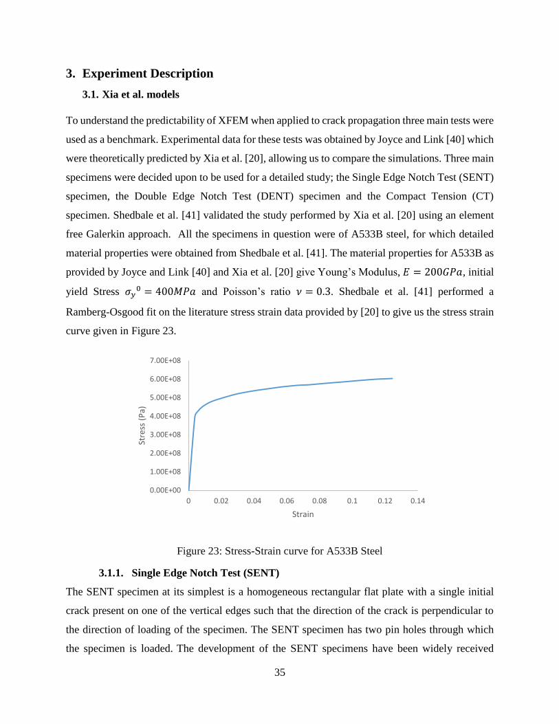
35
3. Experiment Description
3.1. Xia et al. models
To understand the predictability of XFEM when applied to crack propagation three main tests were
used as a benchmark. Experimental data for these tests was obtained by Joyce and Link [40] which
were theoretically predicted by Xia et al. [20], allowing us to compare the simulations. Three main
specimens were decided upon to be used for a detailed study; the Single Edge Notch Test (SENT)
specimen, the Double Edge Notch Test (DENT) specimen and the Compact Tension (CT)
specimen. Shedbale et al. [41] validated the study performed by Xia et al. [20] using an element
free Galerkin approach. All the specimens in question were of A533B steel, for which detailed
material properties were obtained from Shedbale et al. [41]. The material properties for A533B as
provided by Joyce and Link [40] and Xia et al. [20] give Young’s Modulus, 𝐸 = 200𝐺𝑃𝑎, initial
yield Stress 𝜎𝑦0 = 400𝑀𝑃𝑎 and Poisson’s ratio 𝜈 = 0.3. Shedbale et al. [41] performed a
Ramberg-Osgood fit on the literature stress strain data provided by [20] to give us the stress strain
curve given in Figure 23.
Figure 23: Stress-Strain curve for A533B Steel
3.1.1. Single Edge Notch Test (SENT)
The SENT specimen at its simplest is a homogeneous rectangular flat plate with a single initial
crack present on one of the vertical edges such that the direction of the crack is perpendicular to
the direction of loading of the specimen. The SENT specimen has two pin holes through which
the specimen is loaded. The development of the SENT specimens have been widely received
0.00E+00
1.00E+08
2.00E+08
3.00E+08
4.00E+08
5.00E+08
6.00E+08
7.00E+08
0 0.02 0.04 0.06 0.08 0.1 0.12 0.14
Stre
ss (
Pa)
Strain
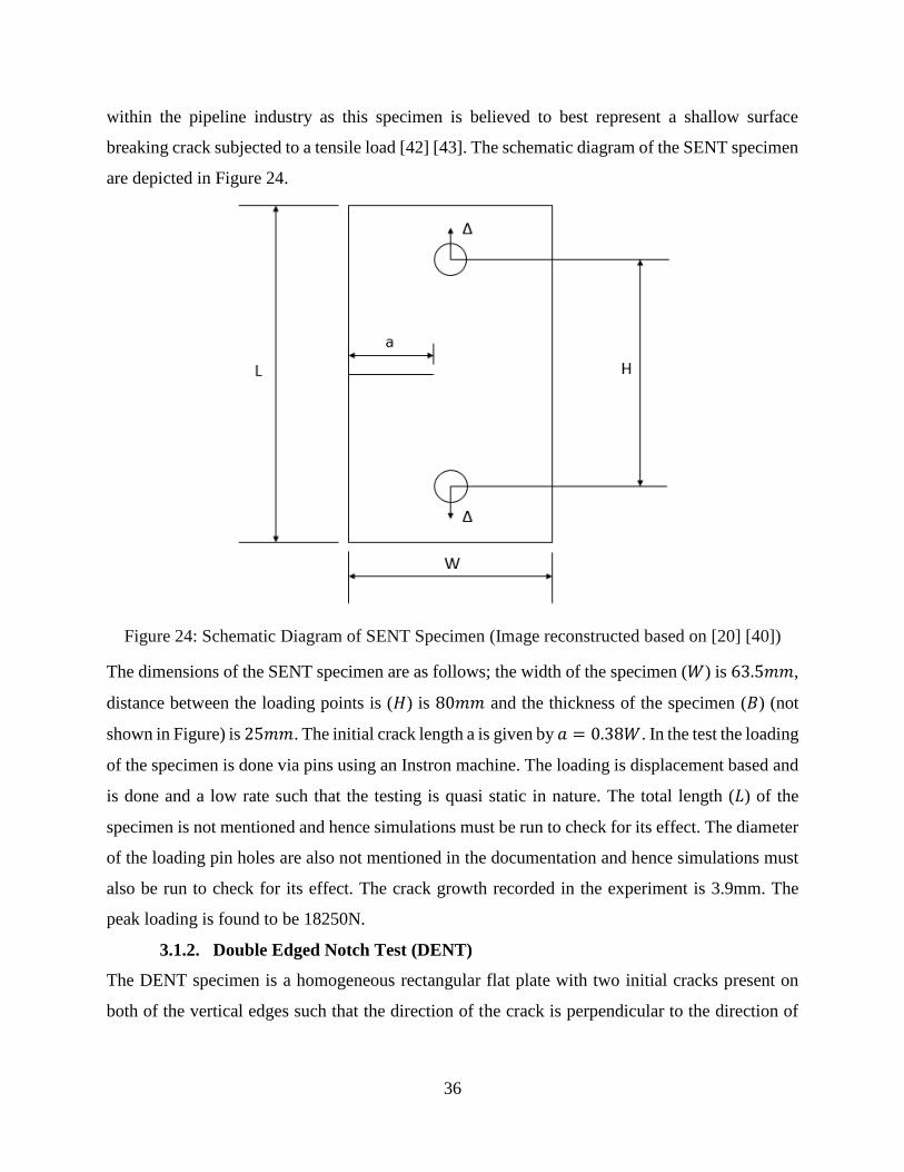
36
within the pipeline industry as this specimen is believed to best represent a shallow surface
breaking crack subjected to a tensile load [42] [43]. The schematic diagram of the SENT specimen
are depicted in Figure 24.
Figure 24: Schematic Diagram of SENT Specimen (Image reconstructed based on [20] [40])
The dimensions of the SENT specimen are as follows; the width of the specimen (𝑊) is 63.5𝑚𝑚,
distance between the loading points is (𝐻) is 80𝑚𝑚 and the thickness of the specimen (𝐵) (not
shown in Figure) is 25𝑚𝑚. The initial crack length a is given by 𝑎 = 0.38𝑊. In the test the loading
of the specimen is done via pins using an Instron machine. The loading is displacement based and
is done and a low rate such that the testing is quasi static in nature. The total length (𝐿) of the
specimen is not mentioned and hence simulations must be run to check for its effect. The diameter
of the loading pin holes are also not mentioned in the documentation and hence simulations must
also be run to check for its effect. The crack growth recorded in the experiment is 3.9mm. The
peak loading is found to be 18250N.
3.1.2. Double Edged Notch Test (DENT)
The DENT specimen is a homogeneous rectangular flat plate with two initial cracks present on
both of the vertical edges such that the direction of the crack is perpendicular to the direction of
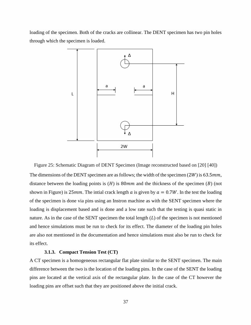
37
loading of the specimen. Both of the cracks are collinear. The DENT specimen has two pin holes
through which the specimen is loaded.
Figure 25: Schematic Diagram of DENT Specimen (Image reconstructed based on [20] [40])
The dimensions of the DENT specimen are as follows; the width of the specimen (2𝑊) is 63.5𝑚𝑚,
distance between the loading points is (𝐻) is 80𝑚𝑚 and the thickness of the specimen (𝐵) (not
shown in Figure) is 25𝑚𝑚. The intial crack length 𝑎 is given by 𝑎 = 0.7𝑊. In the test the loading
of the specimen is done via pins using an Instron machine as with the SENT specimen where the
loading is displacement based and is done and a low rate such that the testing is quasi static in
nature. As in the case of the SENT specimen the total length (𝐿) of the specimen is not mentioned
and hence simulations must be run to check for its effect. The diameter of the loading pin holes
are also not mentioned in the documentation and hence simulations must also be run to check for
its effect.
3.1.3. Compact Tension Test (CT)
A CT specimen is a homogeneous rectangular flat plate similar to the SENT specimen. The main
difference between the two is the location of the loading pins. In the case of the SENT the loading
pins are located at the vertical axis of the rectangular plate. In the case of the CT however the
loading pins are offset such that they are positioned above the initial crack.
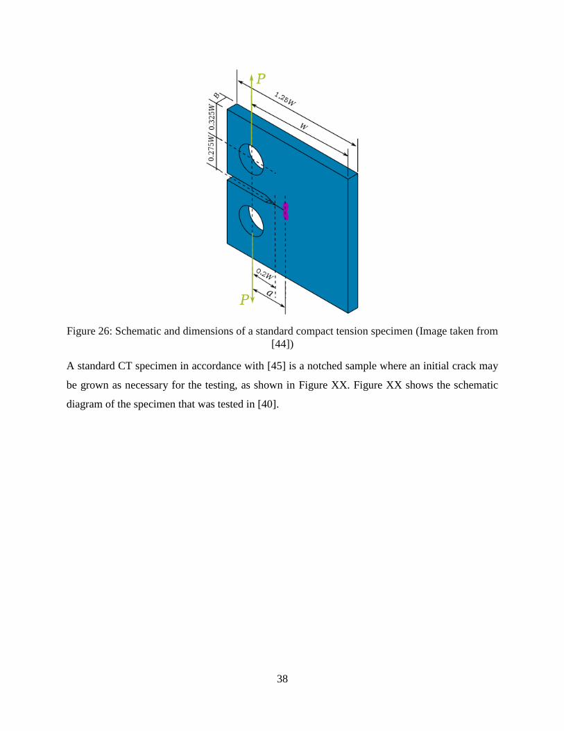
38
Figure 26: Schematic and dimensions of a standard compact tension specimen (Image taken from
[44])
A standard CT specimen in accordance with [45] is a notched sample where an initial crack may
be grown as necessary for the testing, as shown in Figure XX. Figure XX shows the schematic
diagram of the specimen that was tested in [40].
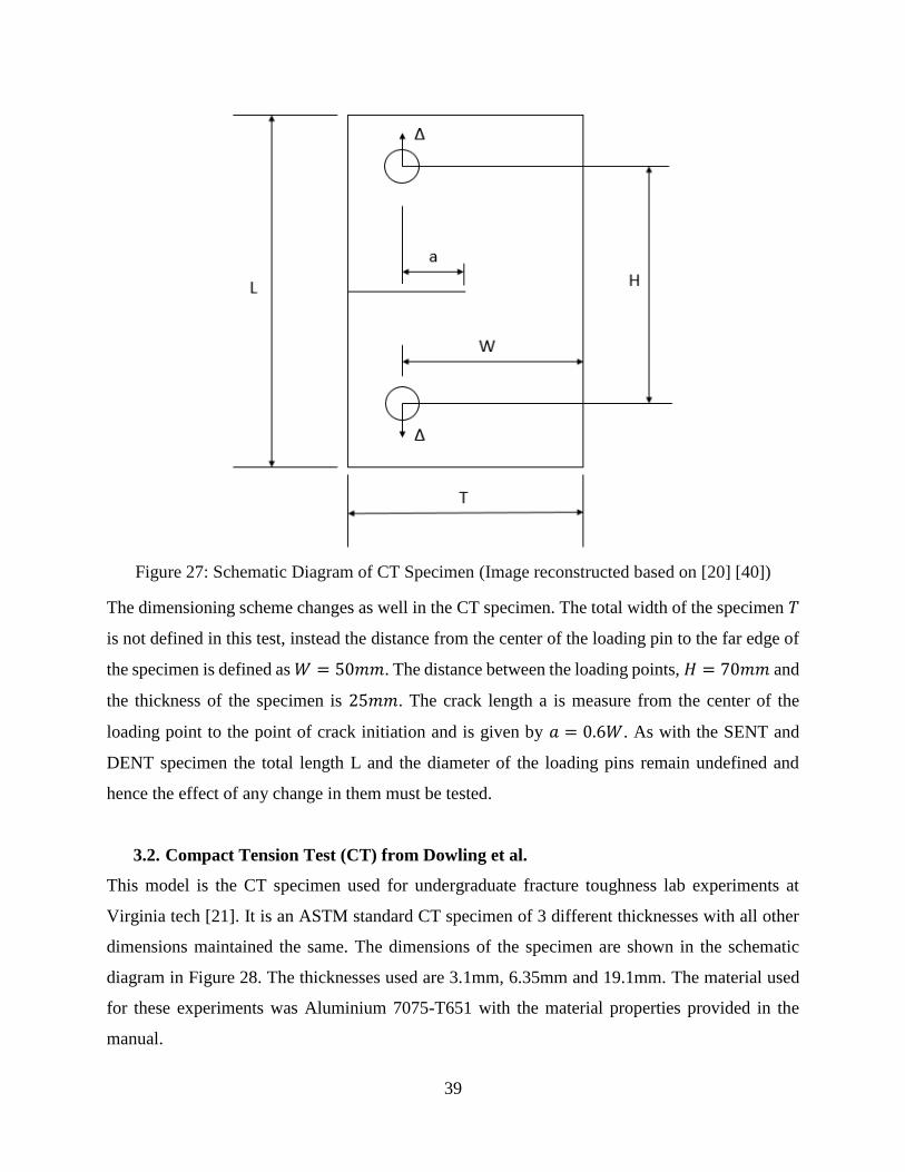
39
Figure 27: Schematic Diagram of CT Specimen (Image reconstructed based on [20] [40])
The dimensioning scheme changes as well in the CT specimen. The total width of the specimen 𝑇
is not defined in this test, instead the distance from the center of the loading pin to the far edge of
the specimen is defined as 𝑊 = 50𝑚𝑚. The distance between the loading points, 𝐻 = 70𝑚𝑚 and
the thickness of the specimen is 25𝑚𝑚. The crack length a is measure from the center of the
loading point to the point of crack initiation and is given by 𝑎 = 0.6𝑊. As with the SENT and
DENT specimen the total length L and the diameter of the loading pins remain undefined and
hence the effect of any change in them must be tested.
3.2. Compact Tension Test (CT) from Dowling et al.
This model is the CT specimen used for undergraduate fracture toughness lab experiments at
Virginia tech [21]. It is an ASTM standard CT specimen of 3 different thicknesses with all other
dimensions maintained the same. The dimensions of the specimen are shown in the schematic
diagram in Figure 28. The thicknesses used are 3.1mm, 6.35mm and 19.1mm. The material used
for these experiments was Aluminium 7075-T651 with the material properties provided in the
manual.
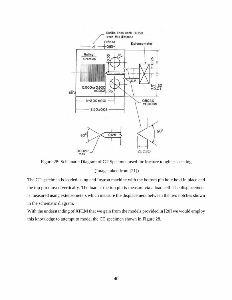
40
Figure 28: Schematic Diagram of CT Specimen used for fracture toughness testing
(Image taken from [21])
The CT specimen is loaded using and Instron machine with the bottom pin hole held in place and
the top pin moved vertically. The load at the top pin is measure via a load cell. The displacement
is measured using extensometers which measure the displacement between the two notches shown
in the schematic diagram.
With the understanding of XFEM that we gain from the models provided in [20] we would employ
this knowledge to attempt to model the CT specimen shown in Figure 28.
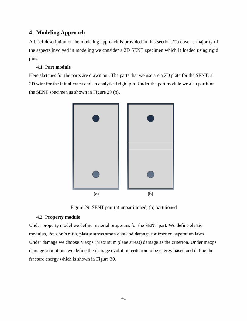
41
4. Modeling Approach
A brief description of the modeling approach is provided in this section. To cover a majority of
the aspects involved in modeling we consider a 2D SENT specimen which is loaded using rigid
pins.
4.1. Part module
Here sketches for the parts are drawn out. The parts that we use are a 2D plate for the SENT, a
2D wire for the initial crack and an analytical rigid pin. Under the part module we also partition
the SENT specimen as shown in Figure 29 (b).
Figure 29: SENT part (a) unpartitioned, (b) partitioned
4.2. Property module
Under property model we define material properties for the SENT part. We define elastic
modulus, Poisson’s ratio, plastic stress strain data and damage for traction separation laws.
Under damage we choose Maxps (Maximum plane stress) damage as the criterion. Under maxps
damage suboptions we define the damage evolution criterion to be energy based and define the
fracture energy which is shown in Figure 30.
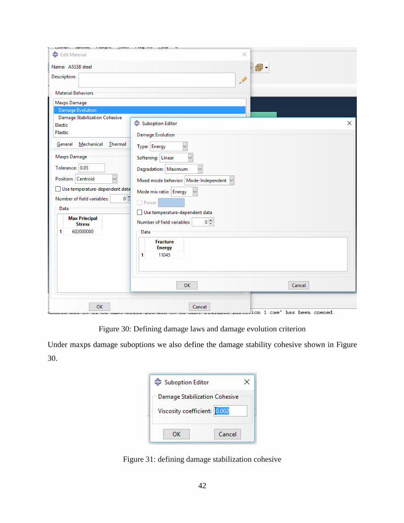
42
Figure 30: Defining damage laws and damage evolution criterion
Under maxps damage suboptions we also define the damage stability cohesive shown in Figure
30.
Figure 31: defining damage stabilization cohesive
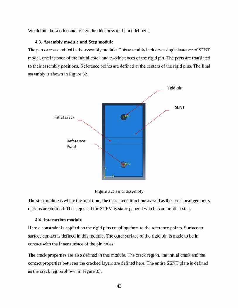
43
We define the section and assign the thickness to the model here.
4.3. Assembly module and Step module
The parts are assembled in the assembly module. This assembly includes a single instance of SENT
model, one instance of the initial crack and two instances of the rigid pin. The parts are translated
to their assembly positions. Reference points are defined at the centers of the rigid pins. The final
assembly is shown in Figure 32.
Figure 32: Final assembly
The step module is where the total time, the incrementation time as well as the non-linear geometry
options are defined. The step used for XFEM is static general which is an implicit step.
4.4. Interaction module
Here a constraint is applied on the rigid pins coupling them to the reference points. Surface to
surface contact is defined in this module. The outer surface of the rigid pin is made to be in
contact with the inner surface of the pin holes.
The crack properties are also defined in this module. The crack region, the initial crack and the
contact properties between the cracked layers are defined here. The entire SENT plate is defined
as the crack region shown in Figure 33.
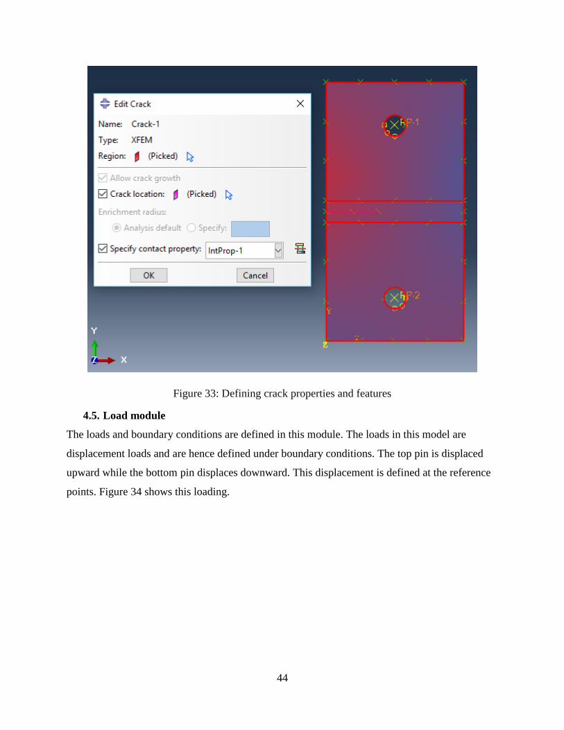
44
Figure 33: Defining crack properties and features
4.5. Load module
The loads and boundary conditions are defined in this module. The loads in this model are
displacement loads and are hence defined under boundary conditions. The top pin is displaced
upward while the bottom pin displaces downward. This displacement is defined at the reference
points. Figure 34 shows this loading.
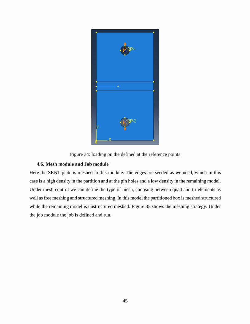
45
Figure 34: loading on the defined at the reference points
4.6. Mesh module and Job module
Here the SENT plate is meshed in this module. The edges are seeded as we need, which in this
case is a high density in the partition and at the pin holes and a low density in the remaining model.
Under mesh control we can define the type of mesh, choosing between quad and tri elements as
well as free meshing and structured meshing. In this model the partitioned box is meshed structured
while the remaining model is unstructured meshed. Figure 35 shows the meshing strategy. Under
the job module the job is defined and run.
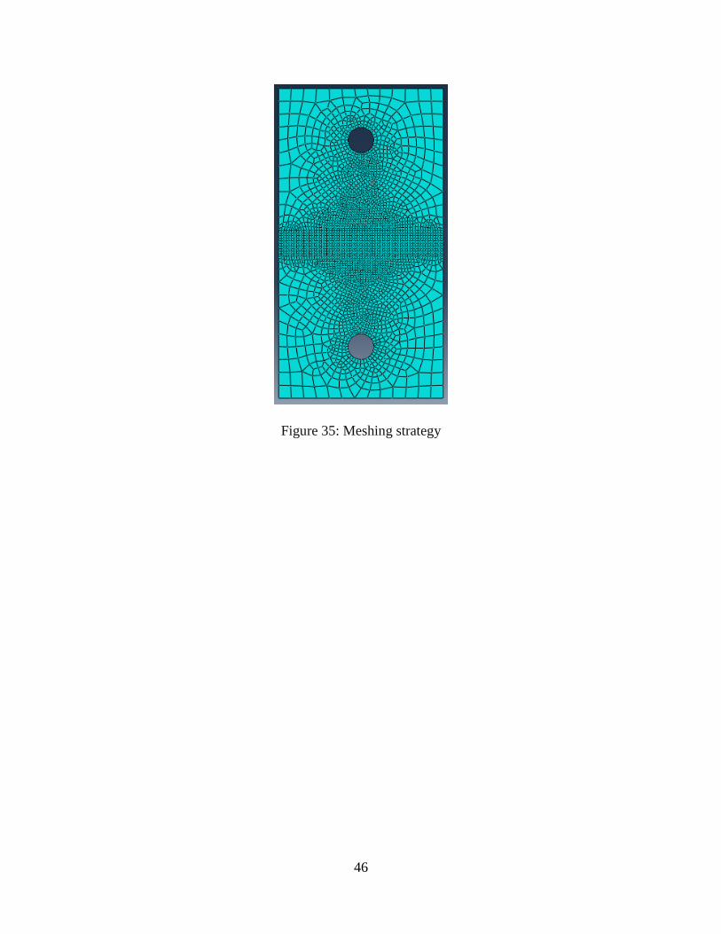
46
Figure 35: Meshing strategy
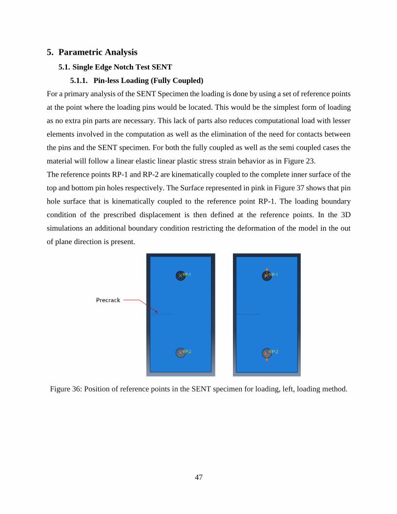
47
5. Parametric Analysis
5.1. Single Edge Notch Test SENT
5.1.1. Pin-less Loading (Fully Coupled)
For a primary analysis of the SENT Specimen the loading is done by using a set of reference points
at the point where the loading pins would be located. This would be the simplest form of loading
as no extra pin parts are necessary. This lack of parts also reduces computational load with lesser
elements involved in the computation as well as the elimination of the need for contacts between
the pins and the SENT specimen. For both the fully coupled as well as the semi coupled cases the
material will follow a linear elastic linear plastic stress strain behavior as in Figure 23.
The reference points RP-1 and RP-2 are kinematically coupled to the complete inner surface of the
top and bottom pin holes respectively. The Surface represented in pink in Figure 37 shows that pin
hole surface that is kinematically coupled to the reference point RP-1. The loading boundary
condition of the prescribed displacement is then defined at the reference points. In the 3D
simulations an additional boundary condition restricting the deformation of the model in the out
of plane direction is present.
Figure 36: Position of reference points in the SENT specimen for loading, left, loading method.
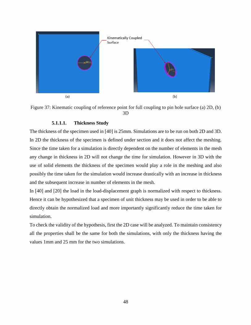
48
Figure 37: Kinematic coupling of reference point for full coupling to pin hole surface (a) 2D, (b)
3D
5.1.1.1. Thickness Study
The thickness of the specimen used in [40] is 25mm. Simulations are to be run on both 2D and 3D.
In 2D the thickness of the specimen is defined under section and it does not affect the meshing.
Since the time taken for a simulation is directly dependent on the number of elements in the mesh
any change in thickness in 2D will not change the time for simulation. However in 3D with the
use of solid elements the thickness of the specimen would play a role in the meshing and also
possibly the time taken for the simulation would increase drastically with an increase in thickness
and the subsequent increase in number of elements in the mesh.
In [40] and [20] the load in the load-displacement graph is normalized with respect to thickness.
Hence it can be hypothesized that a specimen of unit thickness may be used in order to be able to
directly obtain the normalized load and more importantly significantly reduce the time taken for
simulation.
To check the validity of the hypothesis, first the 2D case will be analyzed. To maintain consistency
all the properties shall be the same for both the simulations, with only the thickness having the
values 1mm and 25 mm for the two simulations.
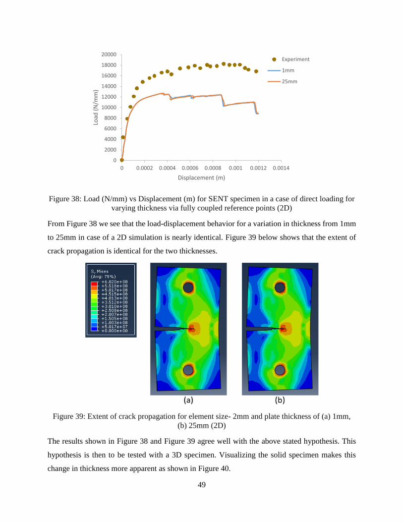
49
Figure 38: Load (N/mm) vs Displacement (m) for SENT specimen in a case of direct loading for
varying thickness via fully coupled reference points (2D)
From Figure 38 we see that the load-displacement behavior for a variation in thickness from 1mm
to 25mm in case of a 2D simulation is nearly identical. Figure 39 below shows that the extent of
crack propagation is identical for the two thicknesses.
Figure 39: Extent of crack propagation for element size- 2mm and plate thickness of (a) 1mm,
(b) 25mm (2D)
The results shown in Figure 38 and Figure 39 agree well with the above stated hypothesis. This
hypothesis is then to be tested with a 3D specimen. Visualizing the solid specimen makes this
change in thickness more apparent as shown in Figure 40.
0 0.0002 0.0004 0.0006 0.0008 0.001 0.0012 0.0014
0
2000
4000
6000
8000
10000
12000
14000
16000
18000
20000
Displacement (m)
Load
(N
/mm
)
Experiment
1mm
25mm
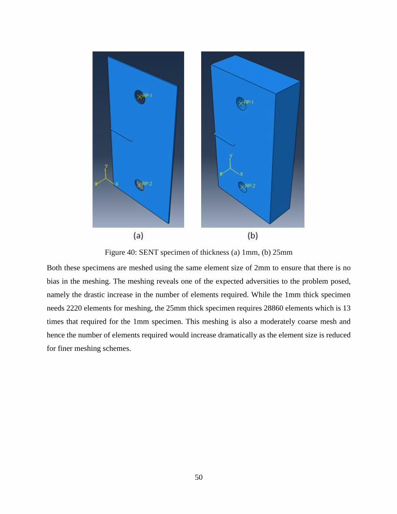
50
Figure 40: SENT specimen of thickness (a) 1mm, (b) 25mm
Both these specimens are meshed using the same element size of 2mm to ensure that there is no
bias in the meshing. The meshing reveals one of the expected adversities to the problem posed,
namely the drastic increase in the number of elements required. While the 1mm thick specimen
needs 2220 elements for meshing, the 25mm thick specimen requires 28860 elements which is 13
times that required for the 1mm specimen. This meshing is also a moderately coarse mesh and
hence the number of elements required would increase dramatically as the element size is reduced
for finer meshing schemes.
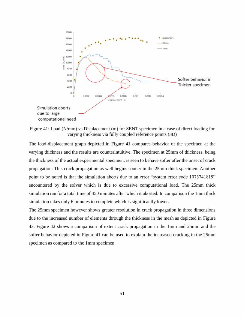
51
Figure 41: Load (N/mm) vs Displacement (m) for SENT specimen in a case of direct loading for
varying thickness via fully coupled reference points (3D)
The load-displacement graph depicted in Figure 41 compares behavior of the specimen at the
varying thickness and the results are counterintuitive. The specimen at 25mm of thickness, being
the thickness of the actual experimental specimen, is seen to behave softer after the onset of crack
propagation. This crack propagation as well begins sooner in the 25mm thick specimen. Another
point to be noted is that the simulation aborts due to an error “system error code 1073741819”
encountered by the solver which is due to excessive computational load. The 25mm thick
simulation ran for a total time of 450 minutes after which it aborted. In comparison the 1mm thick
simulation takes only 6 minutes to complete which is significantly lower.
The 25mm specimen however shows greater resolution in crack propagation in three dimensions
due to the increased number of elements through the thickness in the mesh as depicted in Figure
43. Figure 42 shows a comparison of extent crack propagation in the 1mm and 25mm and the
softer behavior depicted in Figure 41 can be used to explain the increased cracking in the 25mm
specimen as compared to the 1mm specimen.
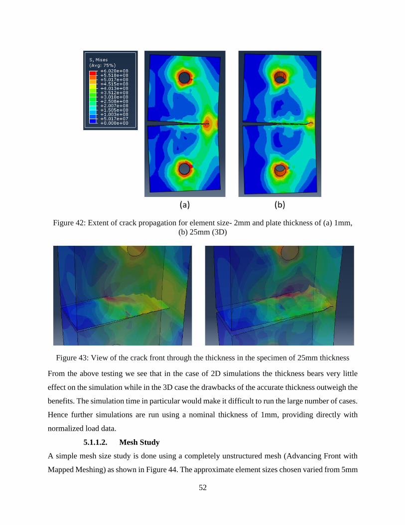
52
Figure 42: Extent of crack propagation for element size- 2mm and plate thickness of (a) 1mm,
(b) 25mm (3D)
Figure 43: View of the crack front through the thickness in the specimen of 25mm thickness
From the above testing we see that in the case of 2D simulations the thickness bears very little
effect on the simulation while in the 3D case the drawbacks of the accurate thickness outweigh the
benefits. The simulation time in particular would make it difficult to run the large number of cases.
Hence further simulations are run using a nominal thickness of 1mm, providing directly with
normalized load data.
5.1.1.2. Mesh Study
A simple mesh size study is done using a completely unstructured mesh (Advancing Front with
Mapped Meshing) as shown in Figure 44. The approximate element sizes chosen varied from 5mm
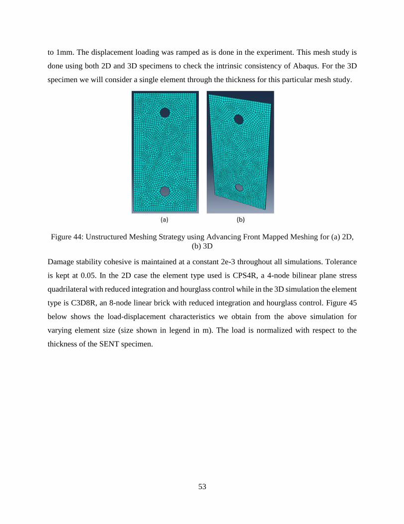
53
to 1mm. The displacement loading was ramped as is done in the experiment. This mesh study is
done using both 2D and 3D specimens to check the intrinsic consistency of Abaqus. For the 3D
specimen we will consider a single element through the thickness for this particular mesh study.
Figure 44: Unstructured Meshing Strategy using Advancing Front Mapped Meshing for (a) 2D,
(b) 3D
Damage stability cohesive is maintained at a constant 2e-3 throughout all simulations. Tolerance
is kept at 0.05. In the 2D case the element type used is CPS4R, a 4-node bilinear plane stress
quadrilateral with reduced integration and hourglass control while in the 3D simulation the element
type is C3D8R, an 8-node linear brick with reduced integration and hourglass control. Figure 45
below shows the load-displacement characteristics we obtain from the above simulation for
varying element size (size shown in legend in m). The load is normalized with respect to the
thickness of the SENT specimen.
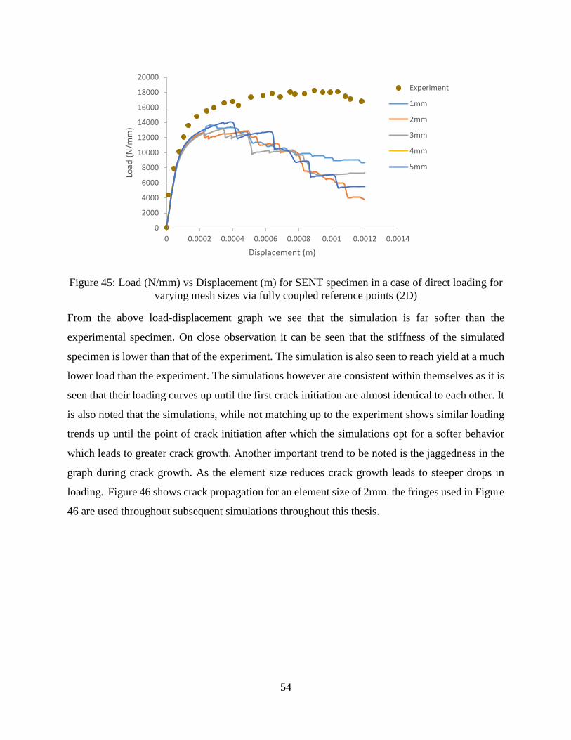
54
Figure 45: Load (N/mm) vs Displacement (m) for SENT specimen in a case of direct loading for
varying mesh sizes via fully coupled reference points (2D)
From the above load-displacement graph we see that the simulation is far softer than the
experimental specimen. On close observation it can be seen that the stiffness of the simulated
specimen is lower than that of the experiment. The simulation is also seen to reach yield at a much
lower load than the experiment. The simulations however are consistent within themselves as it is
seen that their loading curves up until the first crack initiation are almost identical to each other. It
is also noted that the simulations, while not matching up to the experiment shows similar loading
trends up until the point of crack initiation after which the simulations opt for a softer behavior
which leads to greater crack growth. Another important trend to be noted is the jaggedness in the
graph during crack growth. As the element size reduces crack growth leads to steeper drops in
loading. Figure 46 shows crack propagation for an element size of 2mm. the fringes used in Figure
46 are used throughout subsequent simulations throughout this thesis.
0 0.0002 0.0004 0.0006 0.0008 0.001 0.0012 0.0014
0
2000
4000
6000
8000
10000
12000
14000
16000
18000
20000
Displacement (m)
Load
(N
/mm
)
Experiment
1mm
2mm
3mm
4mm
5mm
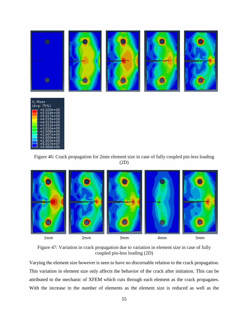
55
Figure 46: Crack propagation for 2mm element size in case of fully coupled pin-less loading
(2D)
Figure 47: Variation in crack propagation due to variation in element size in case of fully
coupled pin-less loading (2D)
Varying the element size however is seen to have no discernable relation to the crack propagation.
This variation in element size only affects the behavior of the crack after initiation. This can be
attributed to the mechanic of XFEM which cuts through each element as the crack propagates.
With the increase in the number of elements as the element size is reduced as well as the
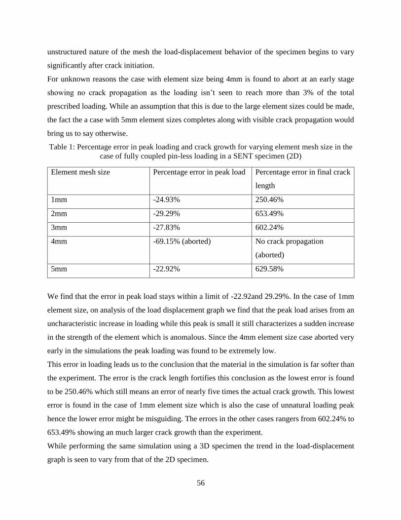
56
unstructured nature of the mesh the load-displacement behavior of the specimen begins to vary
significantly after crack initiation.
For unknown reasons the case with element size being 4mm is found to abort at an early stage
showing no crack propagation as the loading isn’t seen to reach more than 3% of the total
prescribed loading. While an assumption that this is due to the large element sizes could be made,
the fact the a case with 5mm element sizes completes along with visible crack propagation would
bring us to say otherwise.
Table 1: Percentage error in peak loading and crack growth for varying element mesh size in the
case of fully coupled pin-less loading in a SENT specimen (2D)
Element mesh size Percentage error in peak load Percentage error in final crack
length
1mm -24.93% 250.46%
2mm -29.29% 653.49%
3mm -27.83% 602.24%
4mm -69.15% (aborted) No crack propagation
(aborted)
5mm -22.92% 629.58%
We find that the error in peak load stays within a limit of -22.92and 29.29%. In the case of 1mm
element size, on analysis of the load displacement graph we find that the peak load arises from an
uncharacteristic increase in loading while this peak is small it still characterizes a sudden increase
in the strength of the element which is anomalous. Since the 4mm element size case aborted very
early in the simulations the peak loading was found to be extremely low.
This error in loading leads us to the conclusion that the material in the simulation is far softer than
the experiment. The error is the crack length fortifies this conclusion as the lowest error is found
to be 250.46% which still means an error of nearly five times the actual crack growth. This lowest
error is found in the case of 1mm element size which is also the case of unnatural loading peak
hence the lower error might be misguiding. The errors in the other cases rangers from 602.24% to
653.49% showing an much larger crack growth than the experiment.
While performing the same simulation using a 3D specimen the trend in the load-displacement
graph is seen to vary from that of the 2D specimen.
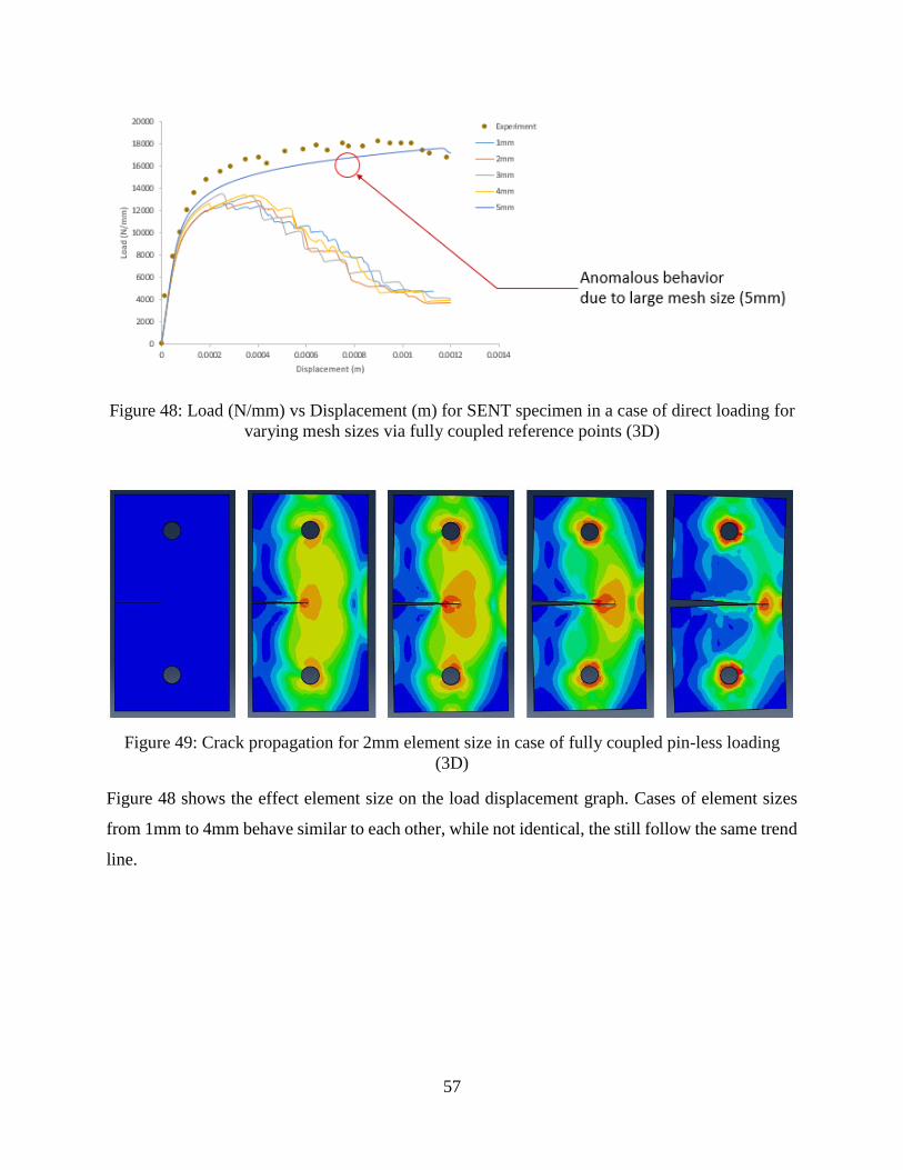
57
Figure 48: Load (N/mm) vs Displacement (m) for SENT specimen in a case of direct loading for
varying mesh sizes via fully coupled reference points (3D)
Figure 49: Crack propagation for 2mm element size in case of fully coupled pin-less loading
(3D)
Figure 48 shows the effect element size on the load displacement graph. Cases of element sizes
from 1mm to 4mm behave similar to each other, while not identical, the still follow the same trend
line.
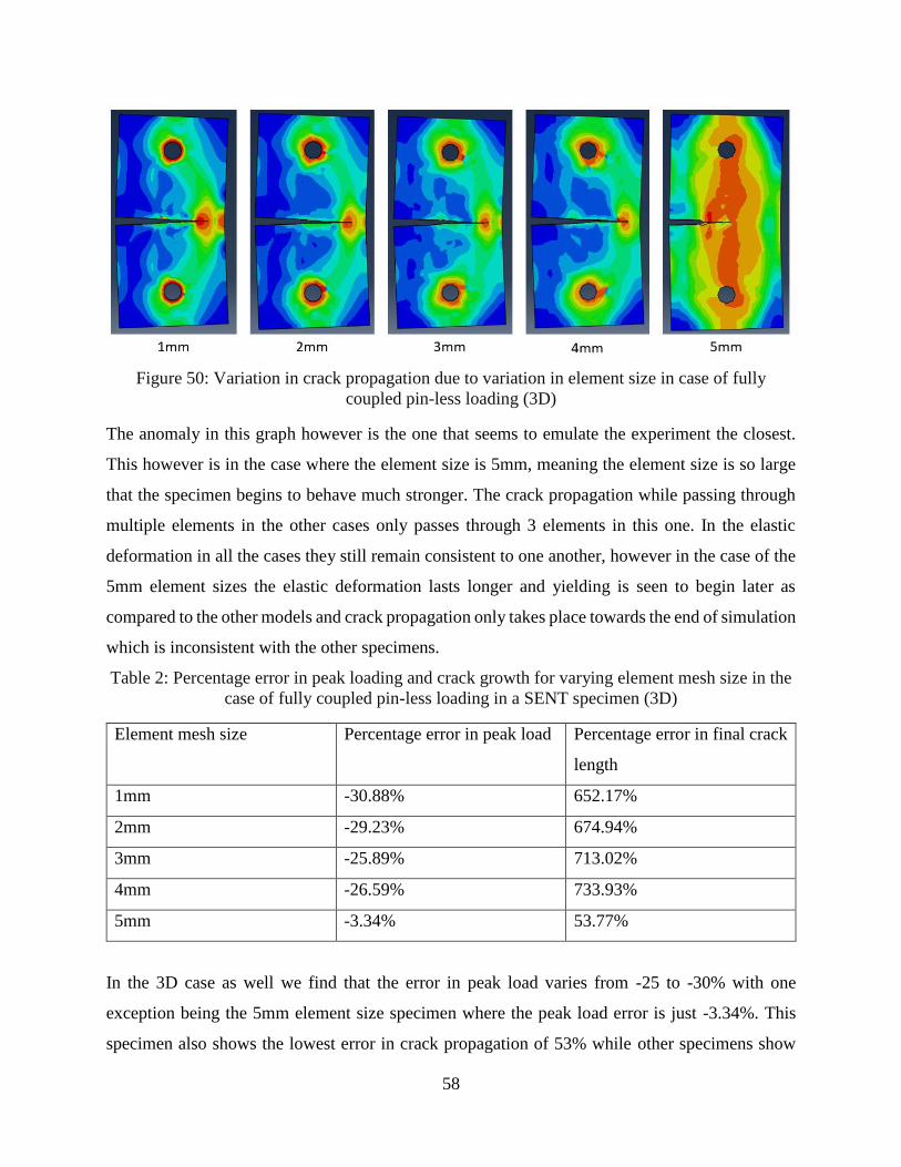
58
Figure 50: Variation in crack propagation due to variation in element size in case of fully
coupled pin-less loading (3D)
The anomaly in this graph however is the one that seems to emulate the experiment the closest.
This however is in the case where the element size is 5mm, meaning the element size is so large
that the specimen begins to behave much stronger. The crack propagation while passing through
multiple elements in the other cases only passes through 3 elements in this one. In the elastic
deformation in all the cases they still remain consistent to one another, however in the case of the
5mm element sizes the elastic deformation lasts longer and yielding is seen to begin later as
compared to the other models and crack propagation only takes place towards the end of simulation
which is inconsistent with the other specimens.
Table 2: Percentage error in peak loading and crack growth for varying element mesh size in the
case of fully coupled pin-less loading in a SENT specimen (3D)
Element mesh size Percentage error in peak load Percentage error in final crack
length
1mm -30.88% 652.17%
2mm -29.23% 674.94%
3mm -25.89% 713.02%
4mm -26.59% 733.93%
5mm -3.34% 53.77%
In the 3D case as well we find that the error in peak load varies from -25 to -30% with one
exception being the 5mm element size specimen where the peak load error is just -3.34%. This
specimen also shows the lowest error in crack propagation of 53% while other specimens show
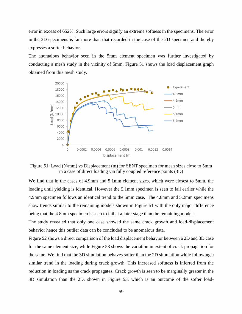
59
error in excess of 652%. Such large errors signify an extreme softness in the specimens. The error
in the 3D specimens is far more than that recorded in the case of the 2D specimen and thereby
expresses a softer behavior.
The anomalous behavior seen in the 5mm element specimen was further investigated by
conducting a mesh study in the vicinity of 5mm. Figure 51 shows the load displacement graph
obtained from this mesh study.
Figure 51: Load (N/mm) vs Displacement (m) for SENT specimen for mesh sizes close to 5mm
in a case of direct loading via fully coupled reference points (3D)
We find that in the cases of 4.9mm and 5.1mm element sizes, which were closest to 5mm, the
loading until yielding is identical. However the 5.1mm specimen is seen to fail earlier while the
4.9mm specimen follows an identical trend to the 5mm case. The 4.8mm and 5.2mm specimens
show trends similar to the remaining models shown in Figure 51 with the only major difference
being that the 4.8mm specimen is seen to fail at a later stage than the remaining models.
The study revealed that only one case showed the same crack growth and load-displacement
behavior hence this outlier data can be concluded to be anomalous data.
Figure 52 shows a direct comparison of the load displacement behavior between a 2D and 3D case
for the same element size, while Figure 53 shows the variation in extent of crack propagation for
the same. We find that the 3D simulation behaves softer than the 2D simulation while following a
similar trend in the loading during crack growth. This increased softness is inferred from the
reduction in loading as the crack propagates. Crack growth is seen to be marginally greater in the
3D simulation than the 2D, shown in Figure 53, which is an outcome of the softer load-
0 0.0002 0.0004 0.0006 0.0008 0.001 0.0012 0.0014
0
2000
4000
6000
8000
10000
12000
14000
16000
18000
20000
Displacement (m)
Load
(N
/mm
)
Experiment
4.8mm
4.9mm
5mm
5.1mm
5.2mm
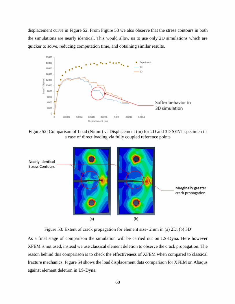
60
displacement curve in Figure 52. From Figure 53 we also observe that the stress contours in both
the simulations are nearly identical. This would allow us to use only 2D simulations which are
quicker to solve, reducing computation time, and obtaining similar results.
Figure 52: Comparison of Load (N/mm) vs Displacement (m) for 2D and 3D SENT specimen in
a case of direct loading via fully coupled reference points
Figure 53: Extent of crack propagation for element size- 2mm in (a) 2D, (b) 3D
As a final stage of comparison the simulation will be carried out on LS-Dyna. Here however
XFEM is not used, instead we use classical element deletion to observe the crack propagation. The
reason behind this comparison is to check the effectiveness of XFEM when compared to classical
fracture mechanics. Figure 54 shows the load displacement data comparison for XFEM on Abaqus
against element deletion in LS-Dyna.
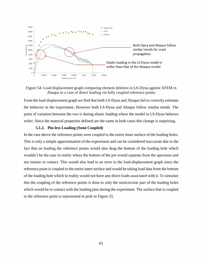
61
Figure 54: Load displacement graph comparing element deletion in LS-Dyna against XFEM in
Abaqus in a case of direct loading via fully coupled reference points
From the load displacement graph we find that both LS-Dyna and Abaqus fail to correctly estimate
the behavior in the experiment. However both LS-Dyna and Abaqus follow similar trends. The
point of variation between the two is during elastic loading where the model in LS-Dyna behaves
softer. Since the material properties defined are the same in both cases this change is surprising.
5.1.2. Pin-less Loading (Semi Coupled)
In the case above the reference points were coupled to the entire inner surface of the loading holes.
This is only a simple approximation of the experiment and can be considered inaccurate due to the
fact that on loading the reference points would also drag the bottom of the loading hole which
wouldn’t be the case in reality where the bottom of the pin would separate from the specimen and
not remain in contact. This would also lead to an error in the load-displacement graph since the
reference point is coupled to the entire inner surface and would be taking load data from the bottom
of the loading hole which in reality would not have any direct loads associated with it. To simulate
this the coupling of the reference points is done to only the semicircular part of the loading holes
which would be in contact with the loading pins during the experiment. The surface that is coupled
to the reference point is represented in pink in Figure 55.
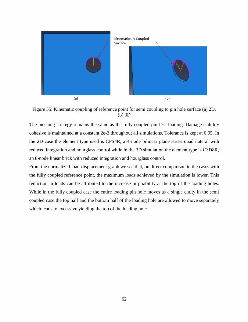
62
Figure 55: Kinematic coupling of reference point for semi coupling to pin hole surface (a) 2D,
(b) 3D
The meshing strategy remains the same as the fully coupled pin-less loading. Damage stability
cohesive is maintained at a constant 2e-3 throughout all simulations. Tolerance is kept at 0.05. In
the 2D case the element type used is CPS4R, a 4-node bilinear plane stress quadrilateral with
reduced integration and hourglass control while in the 3D simulation the element type is C3D8R,
an 8-node linear brick with reduced integration and hourglass control.
From the normalized load-displacement graph we see that, on direct comparison to the cases with
the fully coupled reference point, the maximum loads achieved by the simulation is lower. This
reduction in loads can be attributed to the increase in pliability at the top of the loading holes.
While in the fully coupled case the entire loading pin hole moves as a single entity in the semi
coupled case the top half and the bottom half of the loading hole are allowed to move separately
which leads to excessive yielding the top of the loading hole.
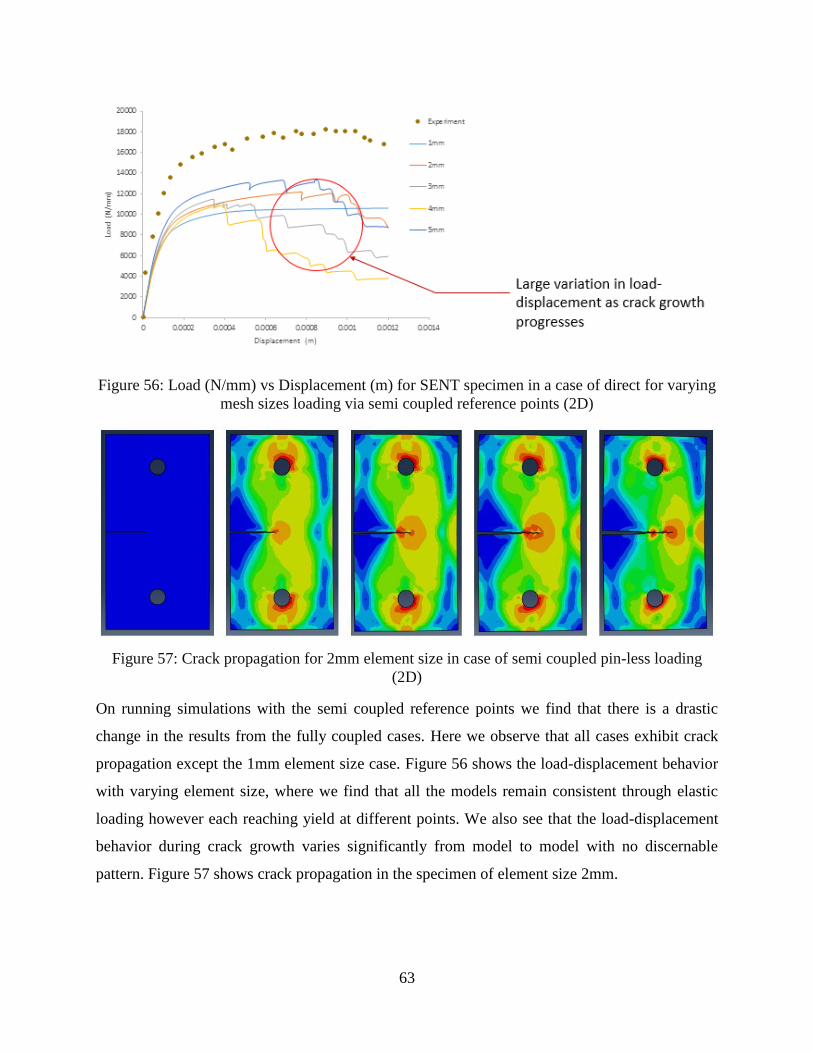
63
Figure 56: Load (N/mm) vs Displacement (m) for SENT specimen in a case of direct for varying
mesh sizes loading via semi coupled reference points (2D)
Figure 57: Crack propagation for 2mm element size in case of semi coupled pin-less loading
(2D)
On running simulations with the semi coupled reference points we find that there is a drastic
change in the results from the fully coupled cases. Here we observe that all cases exhibit crack
propagation except the 1mm element size case. Figure 56 shows the load-displacement behavior
with varying element size, where we find that all the models remain consistent through elastic
loading however each reaching yield at different points. We also see that the load-displacement
behavior during crack growth varies significantly from model to model with no discernable
pattern. Figure 57 shows crack propagation in the specimen of element size 2mm.
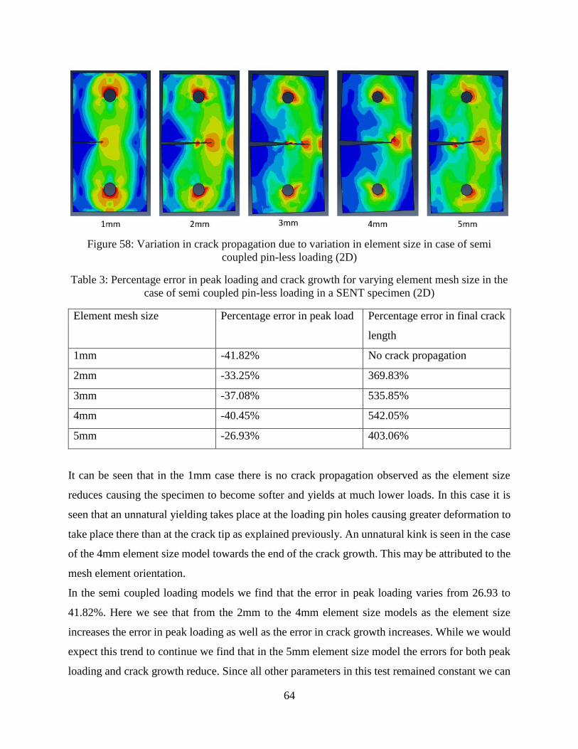
64
Figure 58: Variation in crack propagation due to variation in element size in case of semi
coupled pin-less loading (2D)
Table 3: Percentage error in peak loading and crack growth for varying element mesh size in the
case of semi coupled pin-less loading in a SENT specimen (2D)
Element mesh size Percentage error in peak load Percentage error in final crack
length
1mm -41.82% No crack propagation
2mm -33.25% 369.83%
3mm -37.08% 535.85%
4mm -40.45% 542.05%
5mm -26.93% 403.06%
It can be seen that in the 1mm case there is no crack propagation observed as the element size
reduces causing the specimen to become softer and yields at much lower loads. In this case it is
seen that an unnatural yielding takes place at the loading pin holes causing greater deformation to
take place there than at the crack tip as explained previously. An unnatural kink is seen in the case
of the 4mm element size model towards the end of the crack growth. This may be attributed to the
mesh element orientation.
In the semi coupled loading models we find that the error in peak loading varies from 26.93 to
41.82%. Here we see that from the 2mm to the 4mm element size models as the element size
increases the error in peak loading as well as the error in crack growth increases. While we would
expect this trend to continue we find that in the 5mm element size model the errors for both peak
loading and crack growth reduce. Since all other parameters in this test remained constant we can
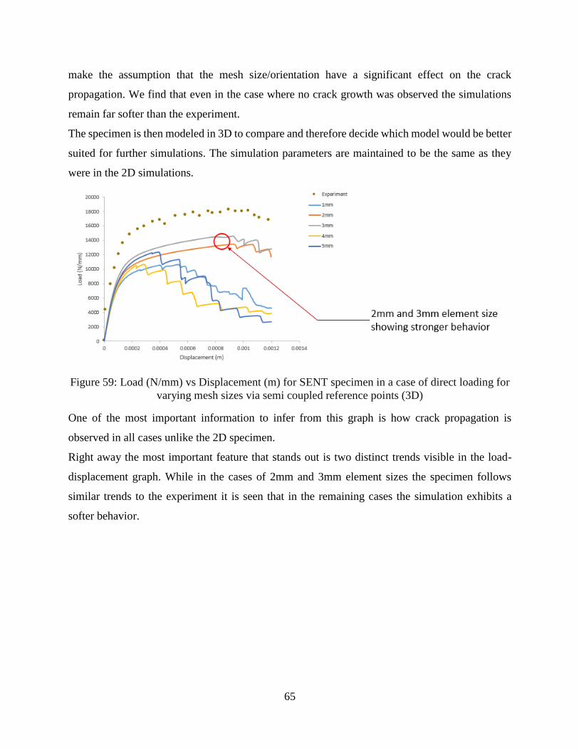
65
make the assumption that the mesh size/orientation have a significant effect on the crack
propagation. We find that even in the case where no crack growth was observed the simulations
remain far softer than the experiment.
The specimen is then modeled in 3D to compare and therefore decide which model would be better
suited for further simulations. The simulation parameters are maintained to be the same as they
were in the 2D simulations.
Figure 59: Load (N/mm) vs Displacement (m) for SENT specimen in a case of direct loading for
varying mesh sizes via semi coupled reference points (3D)
One of the most important information to infer from this graph is how crack propagation is
observed in all cases unlike the 2D specimen.
Right away the most important feature that stands out is two distinct trends visible in the load-
displacement graph. While in the cases of 2mm and 3mm element sizes the specimen follows
similar trends to the experiment it is seen that in the remaining cases the simulation exhibits a
softer behavior.
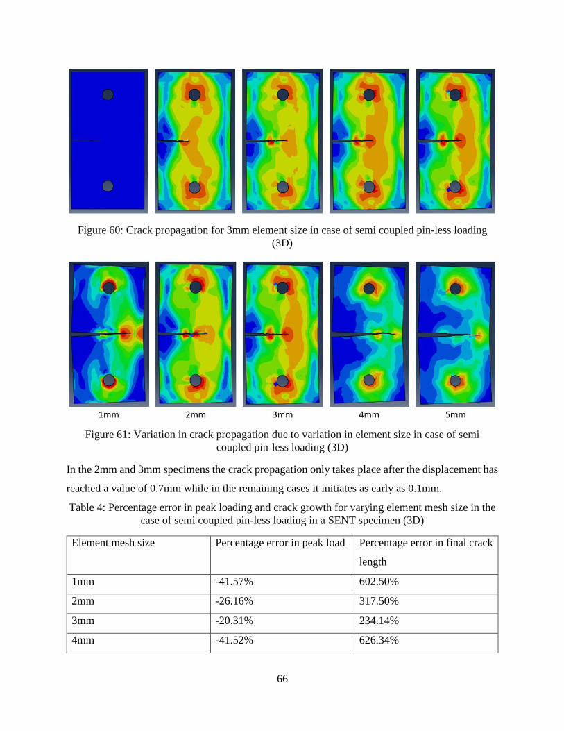
66
Figure 60: Crack propagation for 3mm element size in case of semi coupled pin-less loading
(3D)
Figure 61: Variation in crack propagation due to variation in element size in case of semi
coupled pin-less loading (3D)
In the 2mm and 3mm specimens the crack propagation only takes place after the displacement has
reached a value of 0.7mm while in the remaining cases it initiates as early as 0.1mm.
Table 4: Percentage error in peak loading and crack growth for varying element mesh size in the
case of semi coupled pin-less loading in a SENT specimen (3D)
Element mesh size Percentage error in peak load Percentage error in final crack
length
1mm -41.57% 602.50%
2mm -26.16% 317.50%
3mm -20.31% 234.14%
4mm -41.52% 626.34%
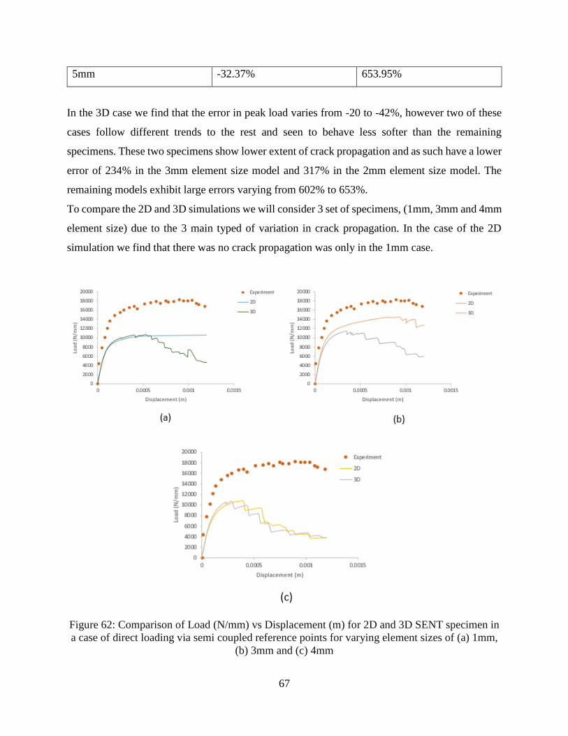
67
5mm -32.37% 653.95%
In the 3D case we find that the error in peak load varies from -20 to -42%, however two of these
cases follow different trends to the rest and seen to behave less softer than the remaining
specimens. These two specimens show lower extent of crack propagation and as such have a lower
error of 234% in the 3mm element size model and 317% in the 2mm element size model. The
remaining models exhibit large errors varying from 602% to 653%.
To compare the 2D and 3D simulations we will consider 3 set of specimens, (1mm, 3mm and 4mm
element size) due to the 3 main typed of variation in crack propagation. In the case of the 2D
simulation we find that there was no crack propagation was only in the 1mm case.
Figure 62: Comparison of Load (N/mm) vs Displacement (m) for 2D and 3D SENT specimen in
a case of direct loading via semi coupled reference points for varying element sizes of (a) 1mm,
(b) 3mm and (c) 4mm
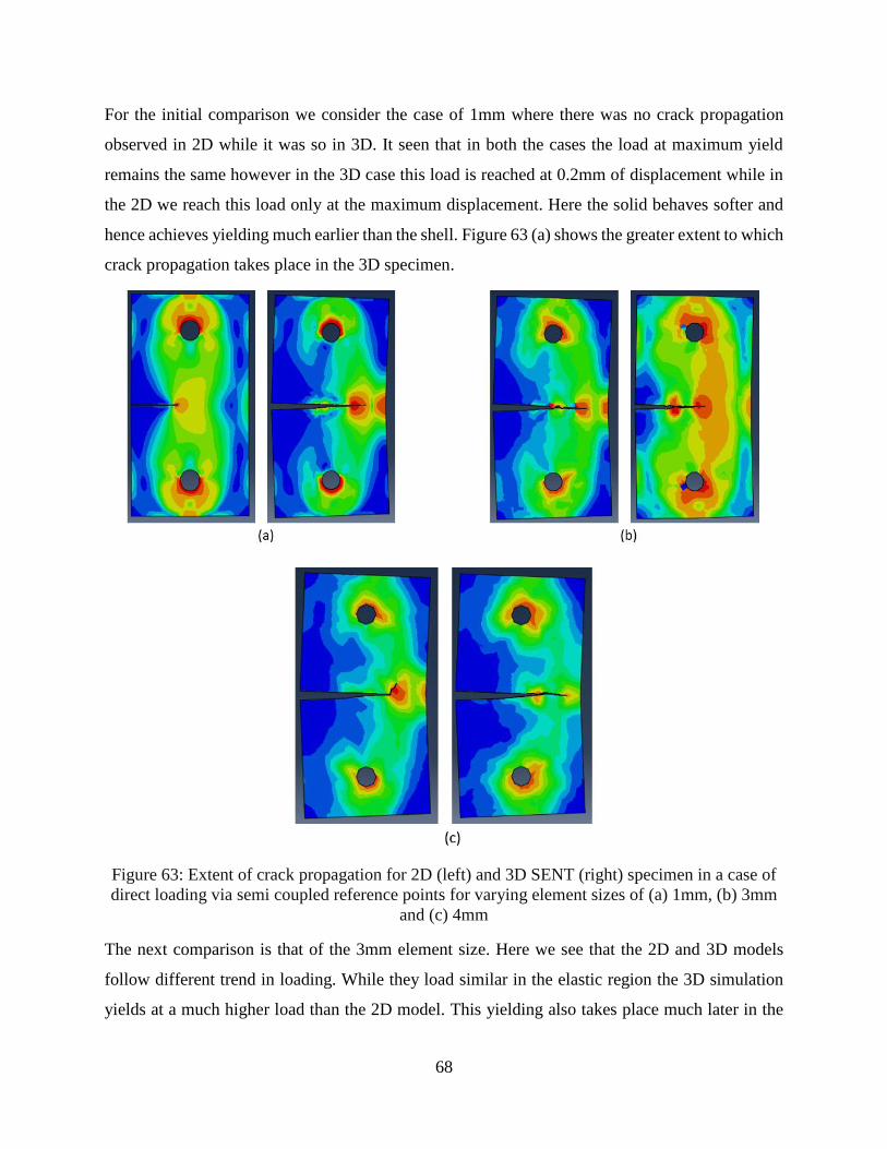
68
For the initial comparison we consider the case of 1mm where there was no crack propagation
observed in 2D while it was so in 3D. It seen that in both the cases the load at maximum yield
remains the same however in the 3D case this load is reached at 0.2mm of displacement while in
the 2D we reach this load only at the maximum displacement. Here the solid behaves softer and
hence achieves yielding much earlier than the shell. Figure 63 (a) shows the greater extent to which
crack propagation takes place in the 3D specimen.
Figure 63: Extent of crack propagation for 2D (left) and 3D SENT (right) specimen in a case of
direct loading via semi coupled reference points for varying element sizes of (a) 1mm, (b) 3mm
and (c) 4mm
The next comparison is that of the 3mm element size. Here we see that the 2D and 3D models
follow different trend in loading. While they load similar in the elastic region the 3D simulation
yields at a much higher load than the 2D model. This yielding also takes place much later in the
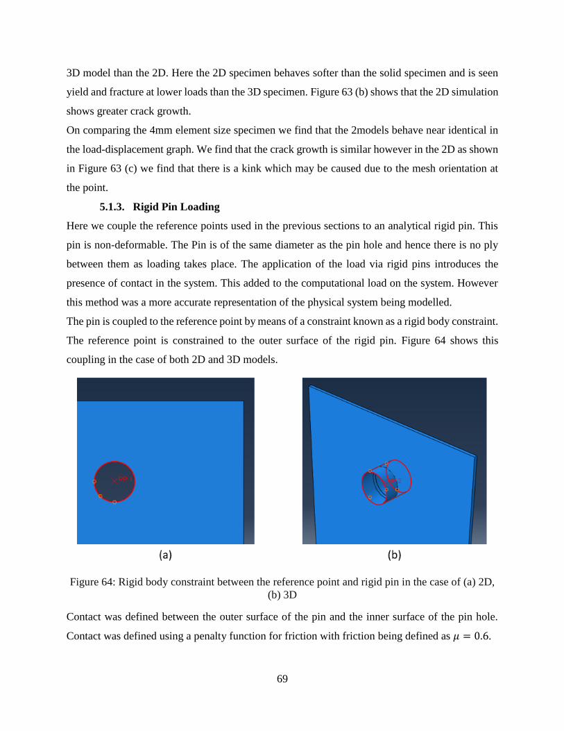
69
3D model than the 2D. Here the 2D specimen behaves softer than the solid specimen and is seen
yield and fracture at lower loads than the 3D specimen. Figure 63 (b) shows that the 2D simulation
shows greater crack growth.
On comparing the 4mm element size specimen we find that the 2models behave near identical in
the load-displacement graph. We find that the crack growth is similar however in the 2D as shown
in Figure 63 (c) we find that there is a kink which may be caused due to the mesh orientation at
the point.
5.1.3. Rigid Pin Loading
Here we couple the reference points used in the previous sections to an analytical rigid pin. This
pin is non-deformable. The Pin is of the same diameter as the pin hole and hence there is no ply
between them as loading takes place. The application of the load via rigid pins introduces the
presence of contact in the system. This added to the computational load on the system. However
this method was a more accurate representation of the physical system being modelled.
The pin is coupled to the reference point by means of a constraint known as a rigid body constraint.
The reference point is constrained to the outer surface of the rigid pin. Figure 64 shows this
coupling in the case of both 2D and 3D models.
Figure 64: Rigid body constraint between the reference point and rigid pin in the case of (a) 2D,
(b) 3D
Contact was defined between the outer surface of the pin and the inner surface of the pin hole.
Contact was defined using a penalty function for friction with friction being defined as 𝜇 = 0.6.
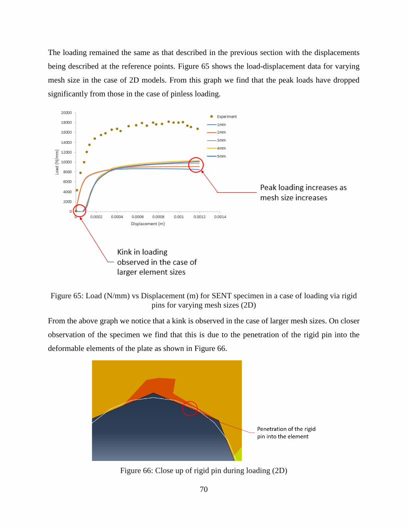
70
The loading remained the same as that described in the previous section with the displacements
being described at the reference points. Figure 65 shows the load-displacement data for varying
mesh size in the case of 2D models. From this graph we find that the peak loads have dropped
significantly from those in the case of pinless loading.
Figure 65: Load (N/mm) vs Displacement (m) for SENT specimen in a case of loading via rigid
pins for varying mesh sizes (2D)
From the above graph we notice that a kink is observed in the case of larger mesh sizes. On closer
observation of the specimen we find that this is due to the penetration of the rigid pin into the
deformable elements of the plate as shown in Figure 66.
Figure 66: Close up of rigid pin during loading (2D)
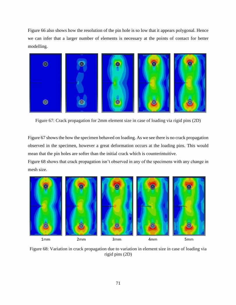
71
Figure 66 also shows how the resolution of the pin hole is so low that it appears polygonal. Hence
we can infer that a larger number of elements is necessary at the points of contact for better
modelling.
Figure 67: Crack propagation for 2mm element size in case of loading via rigid pins (2D)
Figure 67 shows the how the specimen behaved on loading. As we see there is no crack propagation
observed in the specimen, however a great deformation occurs at the loading pins. This would
mean that the pin holes are softer than the initial crack which is counterintuitive.
Figure 68 shows that crack propagation isn’t observed in any of the specimens with any change in
mesh size.
Figure 68: Variation in crack propagation due to variation in element size in case of loading via
rigid pins (2D)
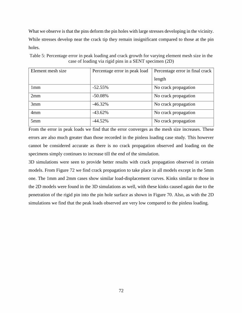
72
What we observe is that the pins deform the pin holes with large stresses developing in the vicinity.
While stresses develop near the crack tip they remain insignificant compared to those at the pin
holes.
Table 5: Percentage error in peak loading and crack growth for varying element mesh size in the
case of loading via rigid pins in a SENT specimen (2D)
Element mesh size Percentage error in peak load Percentage error in final crack
length
1mm -52.55% No crack propagation
2mm -50.08% No crack propagation
3mm -46.32% No crack propagation
4mm -43.62% No crack propagation
5mm -44.52% No crack propagation
From the error in peak loads we find that the error converges as the mesh size increases. These
errors are also much greater than those recorded in the pinless loading case study. This however
cannot be considered accurate as there is no crack propagation observed and loading on the
specimens simply continues to increase till the end of the simulation.
3D simulations were seen to provide better results with crack propagation observed in certain
models. From Figure 72 we find crack propagation to take place in all models except in the 5mm
one. The 1mm and 2mm cases show similar load-displacement curves. Kinks similar to those in
the 2D models were found in the 3D simulations as well, with these kinks caused again due to the
penetration of the rigid pin into the pin hole surface as shown in Figure 70. Also, as with the 2D
simulations we find that the peak loads observed are very low compared to the pinless loading.
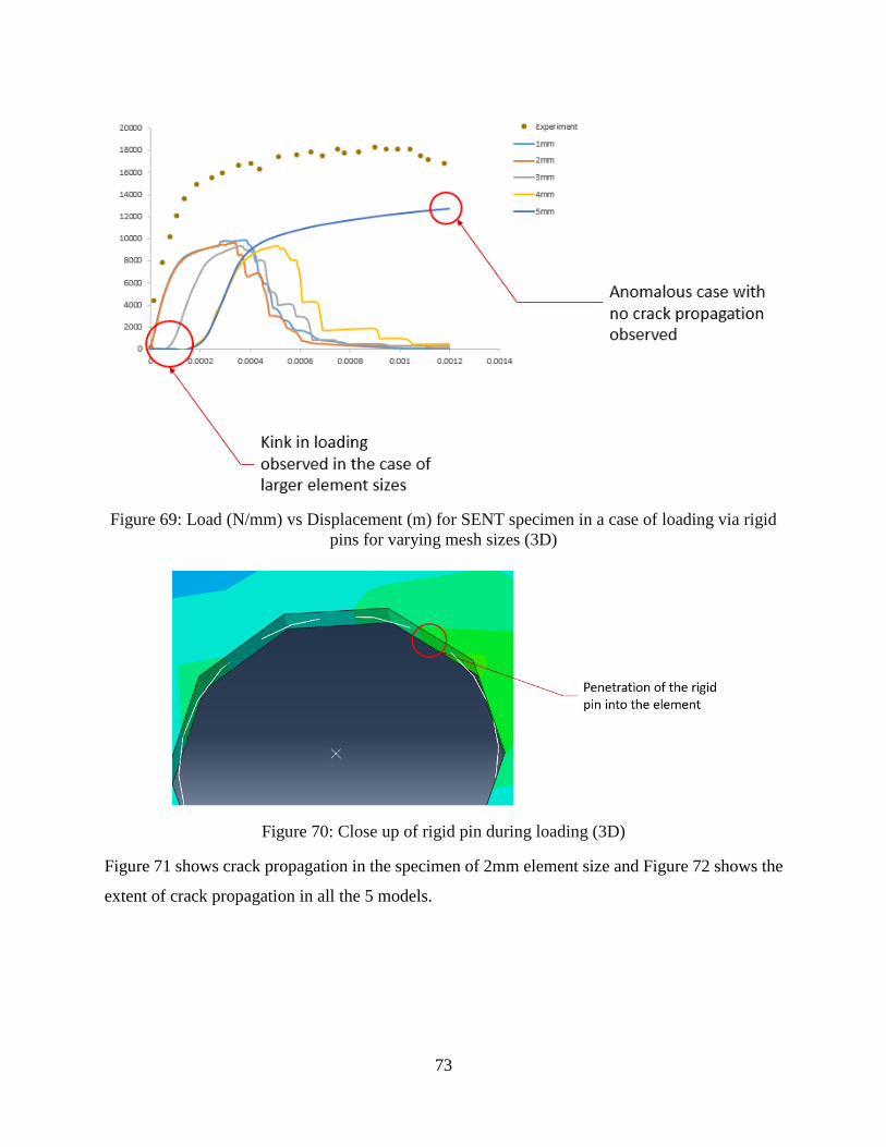
73
Figure 69: Load (N/mm) vs Displacement (m) for SENT specimen in a case of loading via rigid
pins for varying mesh sizes (3D)
Figure 70: Close up of rigid pin during loading (3D)
Figure 71 shows crack propagation in the specimen of 2mm element size and Figure 72 shows the
extent of crack propagation in all the 5 models.
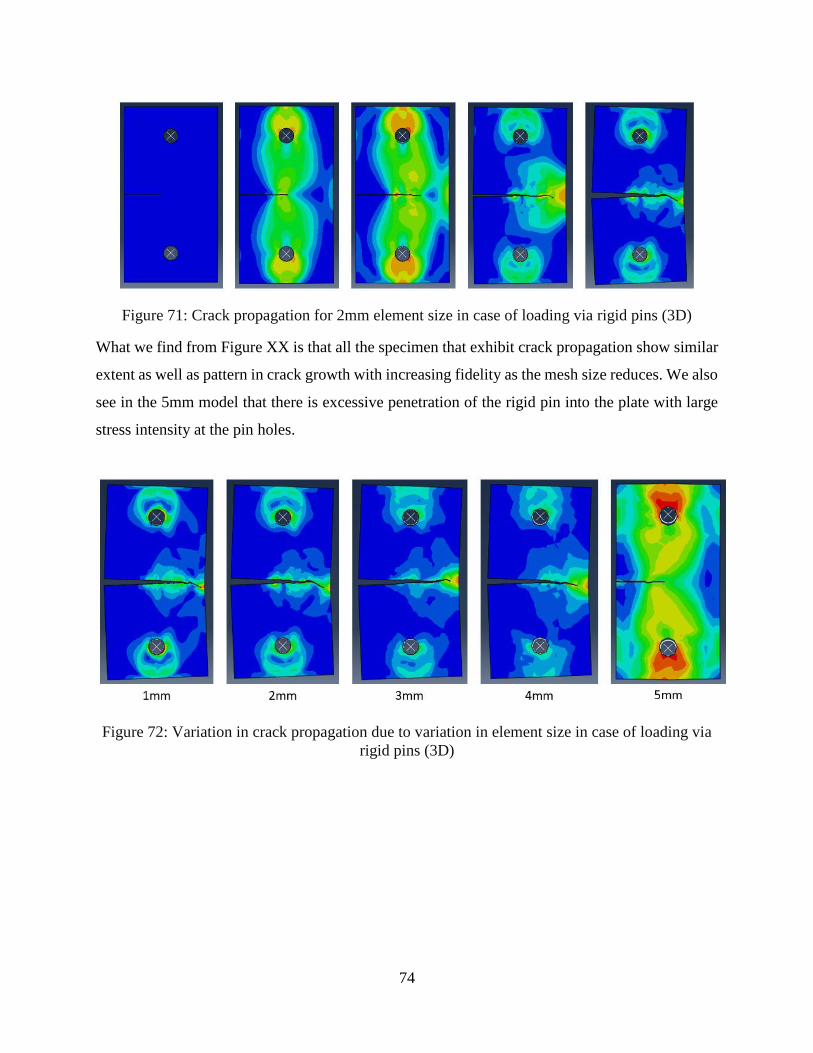
74
Figure 71: Crack propagation for 2mm element size in case of loading via rigid pins (3D)
What we find from Figure XX is that all the specimen that exhibit crack propagation show similar
extent as well as pattern in crack growth with increasing fidelity as the mesh size reduces. We also
see in the 5mm model that there is excessive penetration of the rigid pin into the plate with large
stress intensity at the pin holes.
Figure 72: Variation in crack propagation due to variation in element size in case of loading via
rigid pins (3D)
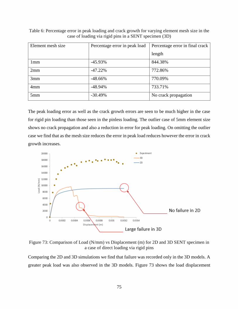
75
Table 6: Percentage error in peak loading and crack growth for varying element mesh size in the
case of loading via rigid pins in a SENT specimen (3D)
Element mesh size Percentage error in peak load Percentage error in final crack
length
1mm -45.93% 844.38%
2mm -47.22% 772.86%
3mm -48.66% 770.09%
4mm -48.94% 733.71%
5mm -30.49% No crack propagation
The peak loading error as well as the crack growth errors are seen to be much higher in the case
for rigid pin loading than those seen in the pinless loading. The outlier case of 5mm element size
shows no crack propagation and also a reduction in error for peak loading. On omitting the outlier
case we find that as the mesh size reduces the error in peak load reduces however the error in crack
growth increases.
Figure 73: Comparison of Load (N/mm) vs Displacement (m) for 2D and 3D SENT specimen in
a case of direct loading via rigid pins
Comparing the 2D and 3D simulations we find that failure was recorded only in the 3D models. A
greater peak load was also observed in the 3D models. Figure 73 shows the load displacement
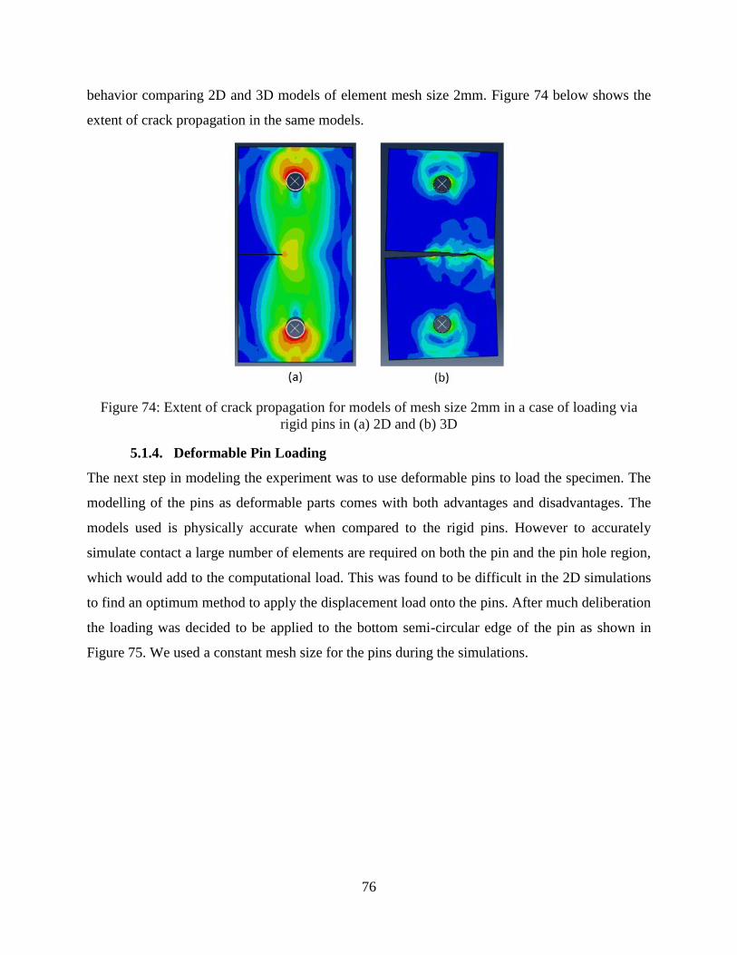
76
behavior comparing 2D and 3D models of element mesh size 2mm. Figure 74 below shows the
extent of crack propagation in the same models.
Figure 74: Extent of crack propagation for models of mesh size 2mm in a case of loading via
rigid pins in (a) 2D and (b) 3D
5.1.4. Deformable Pin Loading
The next step in modeling the experiment was to use deformable pins to load the specimen. The
modelling of the pins as deformable parts comes with both advantages and disadvantages. The
models used is physically accurate when compared to the rigid pins. However to accurately
simulate contact a large number of elements are required on both the pin and the pin hole region,
which would add to the computational load. This was found to be difficult in the 2D simulations
to find an optimum method to apply the displacement load onto the pins. After much deliberation
the loading was decided to be applied to the bottom semi-circular edge of the pin as shown in
Figure 75. We used a constant mesh size for the pins during the simulations.
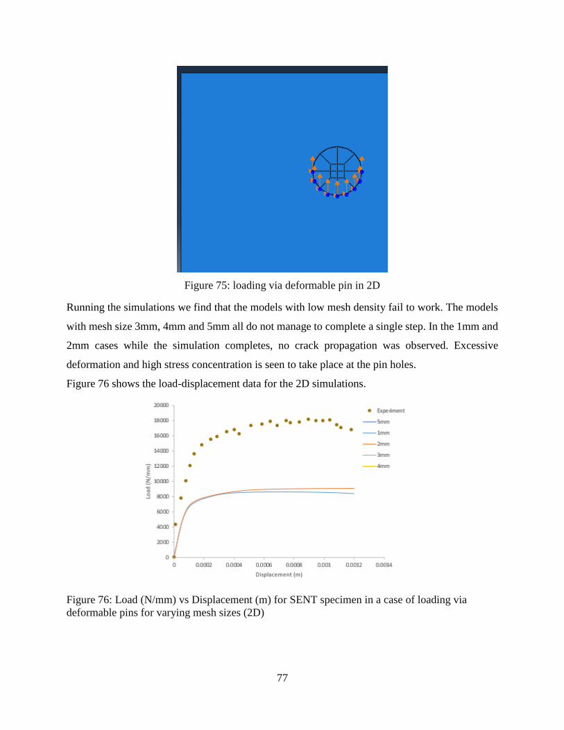
77
Figure 75: loading via deformable pin in 2D
Running the simulations we find that the models with low mesh density fail to work. The models
with mesh size 3mm, 4mm and 5mm all do not manage to complete a single step. In the 1mm and
2mm cases while the simulation completes, no crack propagation was observed. Excessive
deformation and high stress concentration is seen to take place at the pin holes.
Figure 76 shows the load-displacement data for the 2D simulations.
Figure 76: Load (N/mm) vs Displacement (m) for SENT specimen in a case of loading via
deformable pins for varying mesh sizes (2D)
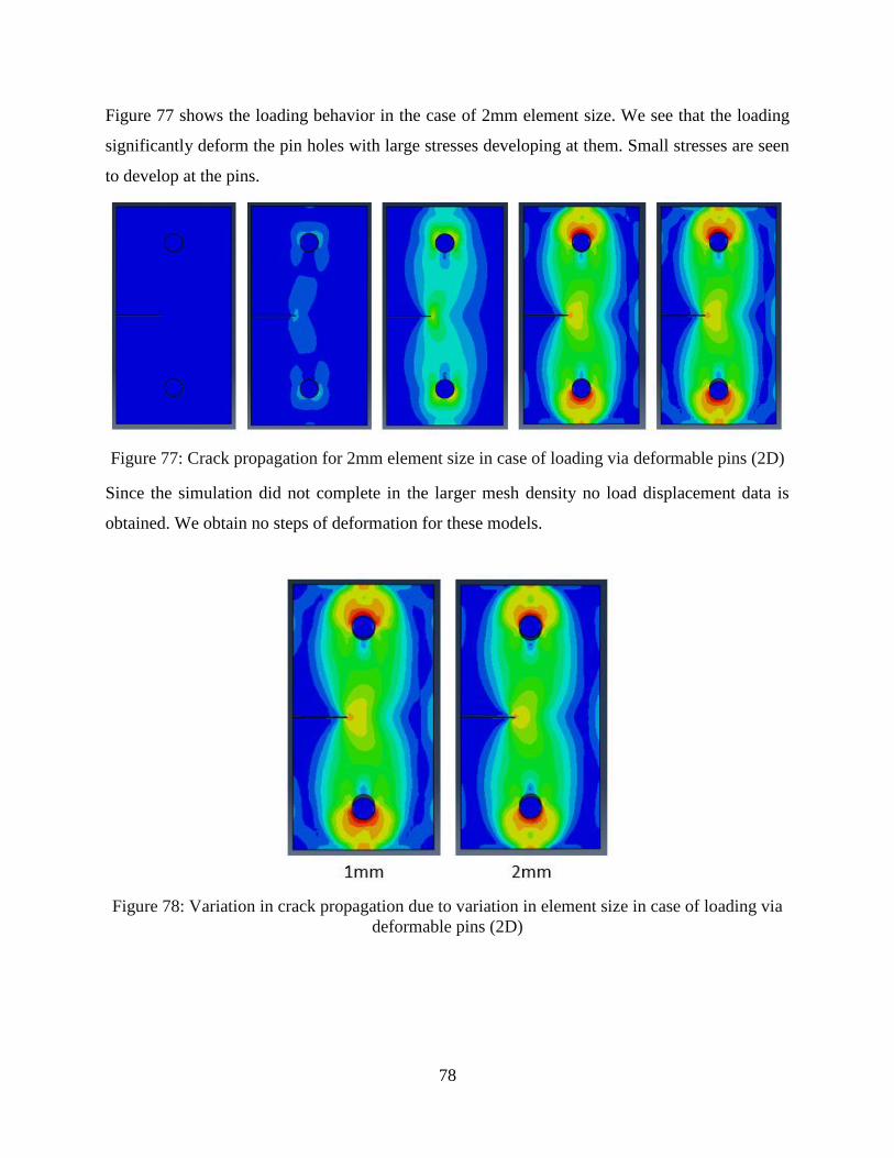
78
Figure 77 shows the loading behavior in the case of 2mm element size. We see that the loading
significantly deform the pin holes with large stresses developing at them. Small stresses are seen
to develop at the pins.
Figure 77: Crack propagation for 2mm element size in case of loading via deformable pins (2D)
Since the simulation did not complete in the larger mesh density no load displacement data is
obtained. We obtain no steps of deformation for these models.
Figure 78: Variation in crack propagation due to variation in element size in case of loading via
deformable pins (2D)
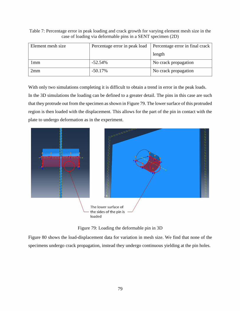
79
Table 7: Percentage error in peak loading and crack growth for varying element mesh size in the
case of loading via deformable pins in a SENT specimen (2D)
Element mesh size Percentage error in peak load Percentage error in final crack
length
1mm -52.54% No crack propagation
2mm -50.17% No crack propagation
With only two simulations completing it is difficult to obtain a trend in error in the peak loads.
In the 3D simulations the loading can be defined to a greater detail. The pins in this case are such
that they protrude out from the specimen as shown in Figure 79. The lower surface of this protruded
region is then loaded with the displacement. This allows for the part of the pin in contact with the
plate to undergo deformation as in the experiment.
Figure 79: Loading the deformable pin in 3D
Figure 80 shows the load-displacement data for variation in mesh size. We find that none of the
specimens undergo crack propagation, instead they undergo continuous yielding at the pin holes.
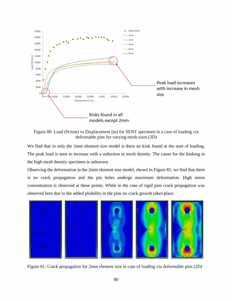
80
Figure 80: Load (N/mm) vs Displacement (m) for SENT specimen in a case of loading via
deformable pins for varying mesh sizes (3D)
We find that in only the 2mm element size model is there no kink found at the start of loading.
The peak load is seen to increase with a reduction in mesh density. The cause for the kinking in
the high mesh density specimen is unknown.
Observing the deformation in the 2mm element size model, shown in Figure 81, we find that there
is no crack propagation and the pin holes undergo maximum deformation. High stress
concentration is observed at these points. While in the case of rigid pins crack propagation was
observed here due to the added pliability in the pins no crack growth takes place.
Figure 81: Crack propagation for 2mm element size in case of loading via deformable pins (2D)
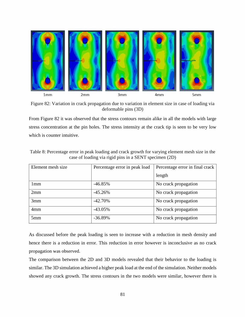
81
Figure 82: Variation in crack propagation due to variation in element size in case of loading via
deformable pins (3D)
From Figure 82 it was observed that the stress contours remain alike in all the models with large
stress concentration at the pin holes. The stress intensity at the crack tip is seen to be very low
which is counter intuitive.
Table 8: Percentage error in peak loading and crack growth for varying element mesh size in the
case of loading via rigid pins in a SENT specimen (2D)
Element mesh size Percentage error in peak load Percentage error in final crack
length
1mm -46.85% No crack propagation
2mm -45.26% No crack propagation
3mm -42.70% No crack propagation
4mm -43.05% No crack propagation
5mm -36.89% No crack propagation
As discussed before the peak loading is seen to increase with a reduction in mesh density and
hence there is a reduction in error. This reduction in error however is inconclusive as no crack
propagation was observed.
The comparison between the 2D and 3D models revealed that their behavior to the loading is
similar. The 3D simulation achieved a higher peak load at the end of the simulation. Neither models
showed any crack growth. The stress contours in the two models were similar, however there is
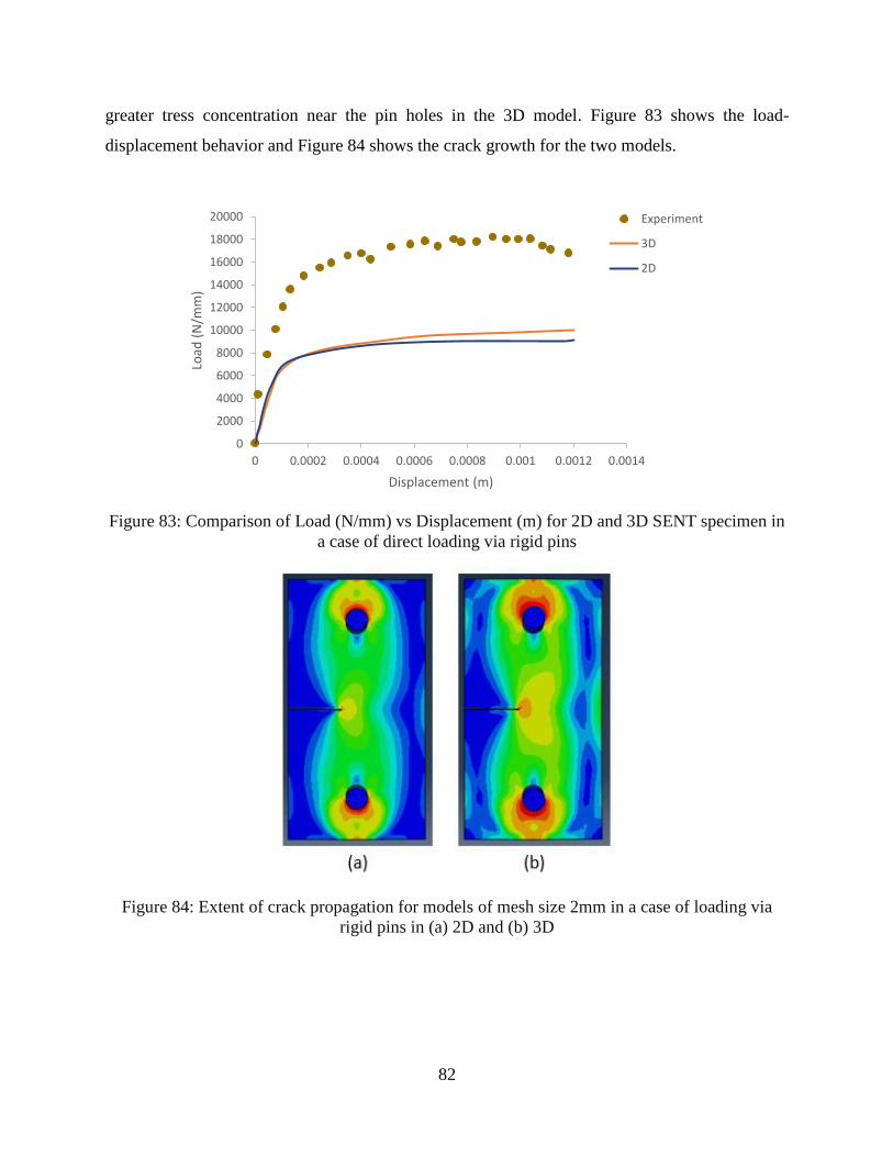
82
greater tress concentration near the pin holes in the 3D model. Figure 83 shows the load-
displacement behavior and Figure 84 shows the crack growth for the two models.
Figure 83: Comparison of Load (N/mm) vs Displacement (m) for 2D and 3D SENT specimen in
a case of direct loading via rigid pins
Figure 84: Extent of crack propagation for models of mesh size 2mm in a case of loading via
rigid pins in (a) 2D and (b) 3D
0 0.0002 0.0004 0.0006 0.0008 0.001 0.0012 0.0014
0
2000
4000
6000
8000
10000
12000
14000
16000
18000
20000
Displacement (m)
Load
(N
/mm
)
Experiment
3D
2D
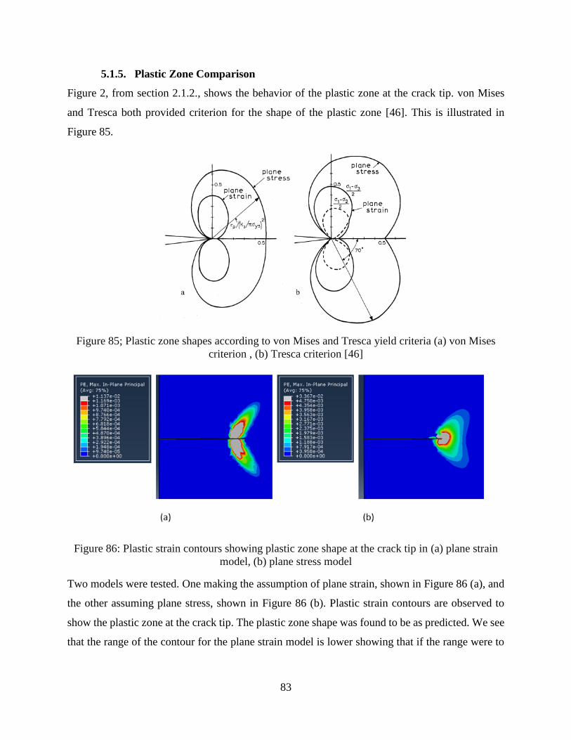
83
5.1.5. Plastic Zone Comparison
Figure 2, from section 2.1.2., shows the behavior of the plastic zone at the crack tip. von Mises
and Tresca both provided criterion for the shape of the plastic zone [46]. This is illustrated in
Figure 85.
Figure 85; Plastic zone shapes according to von Mises and Tresca yield criteria (a) von Mises
criterion , (b) Tresca criterion [46]
Figure 86: Plastic strain contours showing plastic zone shape at the crack tip in (a) plane strain
model, (b) plane stress model
Two models were tested. One making the assumption of plane strain, shown in Figure 86 (a), and
the other assuming plane stress, shown in Figure 86 (b). Plastic strain contours are observed to
show the plastic zone at the crack tip. The plastic zone shape was found to be as predicted. We see
that the range of the contour for the plane strain model is lower showing that if the range were to
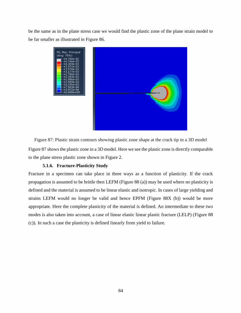
84
be the same as in the plane stress case we would find the plastic zone of the plane strain model to
be far smaller as illustrated in Figure 86.
Figure 87: Plastic strain contours showing plastic zone shape at the crack tip in a 3D model
Figure 87 shows the plastic zone in a 3D model. Here we see the plastic zone is directly comparable
to the plane stress plastic zone shown in Figure 2.
5.1.6. Fracture-Plasticity Study
Fracture in a specimen can take place in three ways as a function of plasticity. If the crack
propagation is assumed to be brittle then LEFM (Figure 88 (a)) may be used where no plasticity is
defined and the material is assumed to be linear elastic and isotropic. In cases of large yielding and
strains LEFM would no longer be valid and hence EPFM (Figure 88X (b)) would be more
appropriate. Here the complete plasticity of the material is defined. An intermediate to these two
modes is also taken into account, a case of linear elastic linear plastic fracture (LELP) (Figure 88
(c)). In such a case the plasticity is defined linearly from yield to failure.
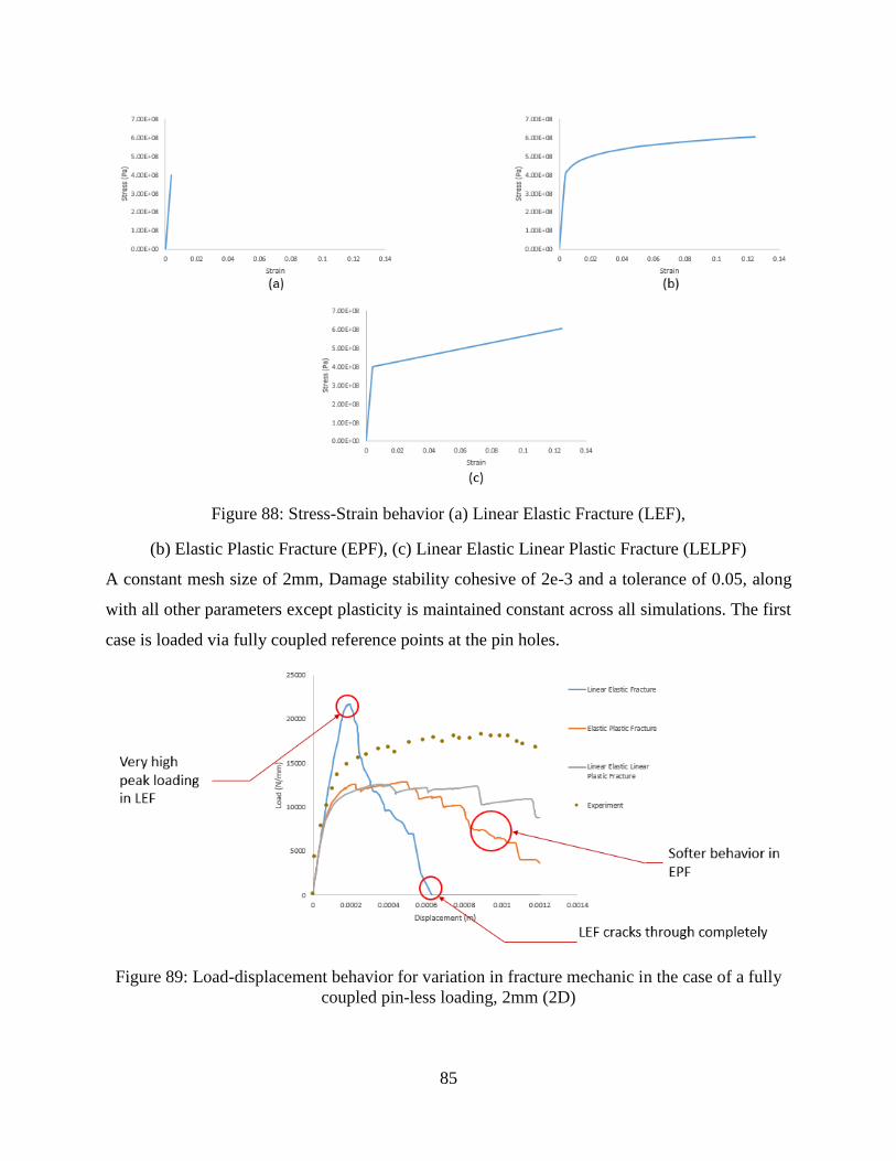
85
Figure 88: Stress-Strain behavior (a) Linear Elastic Fracture (LEF),
(b) Elastic Plastic Fracture (EPF), (c) Linear Elastic Linear Plastic Fracture (LELPF)
A constant mesh size of 2mm, Damage stability cohesive of 2e-3 and a tolerance of 0.05, along
with all other parameters except plasticity is maintained constant across all simulations. The first
case is loaded via fully coupled reference points at the pin holes.
Figure 89: Load-displacement behavior for variation in fracture mechanic in the case of a fully
coupled pin-less loading, 2mm (2D)
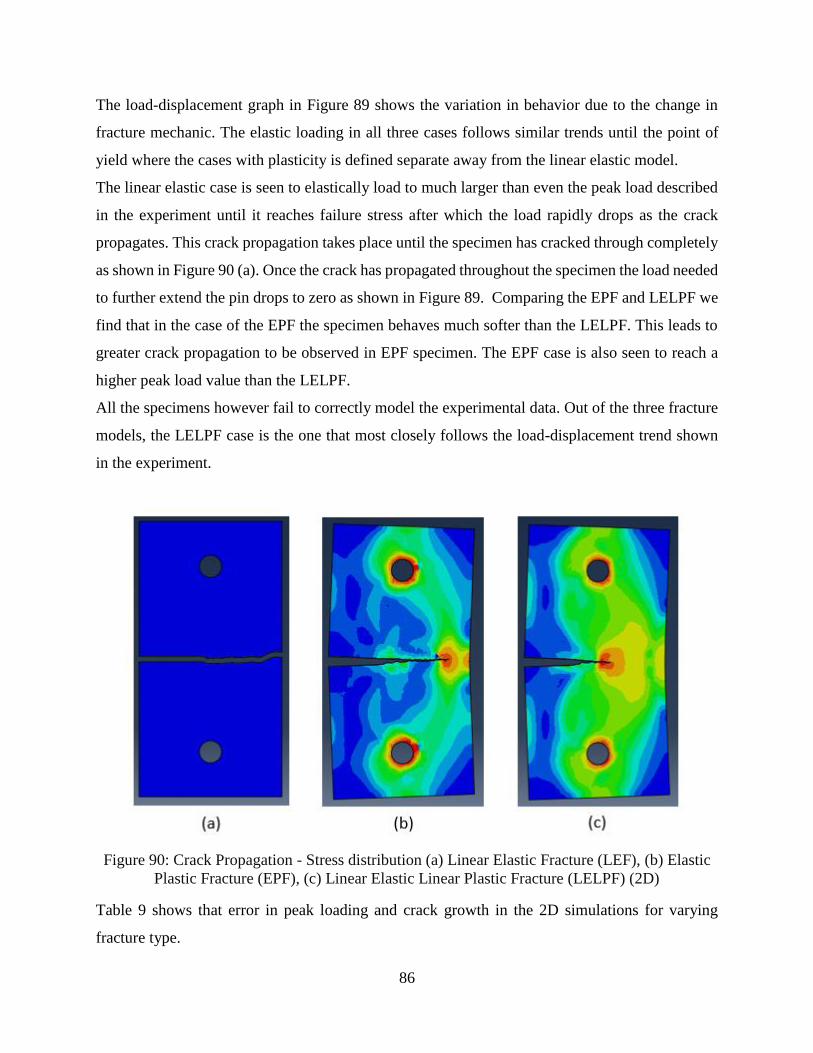
86
The load-displacement graph in Figure 89 shows the variation in behavior due to the change in
fracture mechanic. The elastic loading in all three cases follows similar trends until the point of
yield where the cases with plasticity is defined separate away from the linear elastic model.
The linear elastic case is seen to elastically load to much larger than even the peak load described
in the experiment until it reaches failure stress after which the load rapidly drops as the crack
propagates. This crack propagation takes place until the specimen has cracked through completely
as shown in Figure 90 (a). Once the crack has propagated throughout the specimen the load needed
to further extend the pin drops to zero as shown in Figure 89. Comparing the EPF and LELPF we
find that in the case of the EPF the specimen behaves much softer than the LELPF. This leads to
greater crack propagation to be observed in EPF specimen. The EPF case is also seen to reach a
higher peak load value than the LELPF.
All the specimens however fail to correctly model the experimental data. Out of the three fracture
models, the LELPF case is the one that most closely follows the load-displacement trend shown
in the experiment.
Figure 90: Crack Propagation - Stress distribution (a) Linear Elastic Fracture (LEF), (b) Elastic
Plastic Fracture (EPF), (c) Linear Elastic Linear Plastic Fracture (LELPF) (2D)
Table 9 shows that error in peak loading and crack growth in the 2D simulations for varying
fracture type.
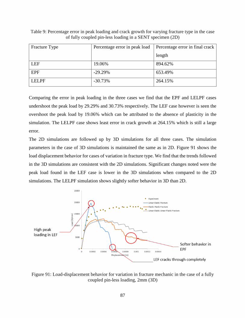
87
Table 9: Percentage error in peak loading and crack growth for varying fracture type in the case
of fully coupled pin-less loading in a SENT specimen (2D)
Fracture Type Percentage error in peak load Percentage error in final crack
length
LEF 19.06% 894.62%
EPF -29.29% 653.49%
LELPF -30.73% 264.15%
Comparing the error in peak loading in the three cases we find that the EPF and LELPF cases
undershoot the peak load by 29.29% and 30.73% respectively. The LEF case however is seen the
overshoot the peak load by 19.06% which can be attributed to the absence of plasticity in the
simulation. The LELPF case shows least error in crack growth at 264.15% which is still a large
error.
The 2D simulations are followed up by 3D simulations for all three cases. The simulation
parameters in the case of 3D simulations is maintained the same as in 2D. Figure 91 shows the
load displacement behavior for cases of variation in fracture type. We find that the trends followed
in the 3D simulations are consistent with the 2D simulations. Significant changes noted were the
peak load found in the LEF case is lower in the 3D simulations when compared to the 2D
simulations. The LELPF simulation shows slightly softer behavior in 3D than 2D.
Figure 91: Load-displacement behavior for variation in fracture mechanic in the case of a fully
coupled pin-less loading, 2mm (3D)
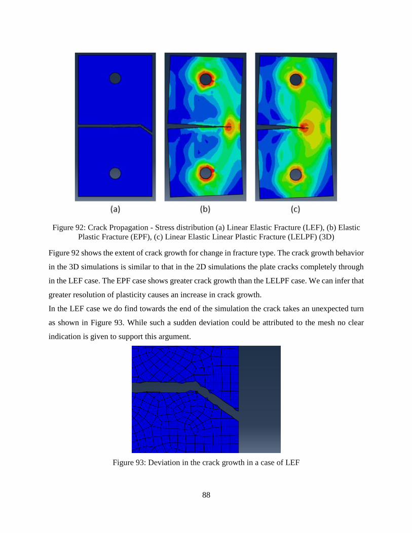
88
Figure 92: Crack Propagation - Stress distribution (a) Linear Elastic Fracture (LEF), (b) Elastic
Plastic Fracture (EPF), (c) Linear Elastic Linear Plastic Fracture (LELPF) (3D)
Figure 92 shows the extent of crack growth for change in fracture type. The crack growth behavior
in the 3D simulations is similar to that in the 2D simulations the plate cracks completely through
in the LEF case. The EPF case shows greater crack growth than the LELPF case. We can infer that
greater resolution of plasticity causes an increase in crack growth.
In the LEF case we do find towards the end of the simulation the crack takes an unexpected turn
as shown in Figure 93. While such a sudden deviation could be attributed to the mesh no clear
indication is given to support this argument.
Figure 93: Deviation in the crack growth in a case of LEF
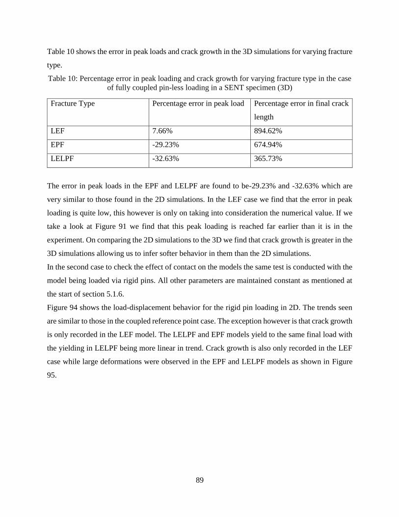
89
Table 10 shows the error in peak loads and crack growth in the 3D simulations for varying fracture
type.
Table 10: Percentage error in peak loading and crack growth for varying fracture type in the case
of fully coupled pin-less loading in a SENT specimen (3D)
Fracture Type Percentage error in peak load Percentage error in final crack
length
LEF 7.66% 894.62%
EPF -29.23% 674.94%
LELPF -32.63% 365.73%
The error in peak loads in the EPF and LELPF are found to be-29.23% and -32.63% which are
very similar to those found in the 2D simulations. In the LEF case we find that the error in peak
loading is quite low, this however is only on taking into consideration the numerical value. If we
take a look at Figure 91 we find that this peak loading is reached far earlier than it is in the
experiment. On comparing the 2D simulations to the 3D we find that crack growth is greater in the
3D simulations allowing us to infer softer behavior in them than the 2D simulations.
In the second case to check the effect of contact on the models the same test is conducted with the
model being loaded via rigid pins. All other parameters are maintained constant as mentioned at
the start of section 5.1.6.
Figure 94 shows the load-displacement behavior for the rigid pin loading in 2D. The trends seen
are similar to those in the coupled reference point case. The exception however is that crack growth
is only recorded in the LEF model. The LELPF and EPF models yield to the same final load with
the yielding in LELPF being more linear in trend. Crack growth is also only recorded in the LEF
case while large deformations were observed in the EPF and LELPF models as shown in Figure
95.
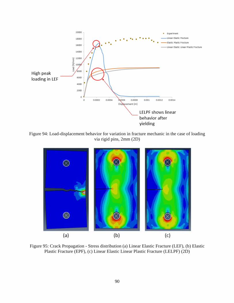
90
Figure 94: Load-displacement behavior for variation in fracture mechanic in the case of loading
via rigid pins, 2mm (2D)
Figure 95: Crack Propagation - Stress distribution (a) Linear Elastic Fracture (LEF), (b) Elastic
Plastic Fracture (EPF), (c) Linear Elastic Linear Plastic Fracture (LELPF) (2D)
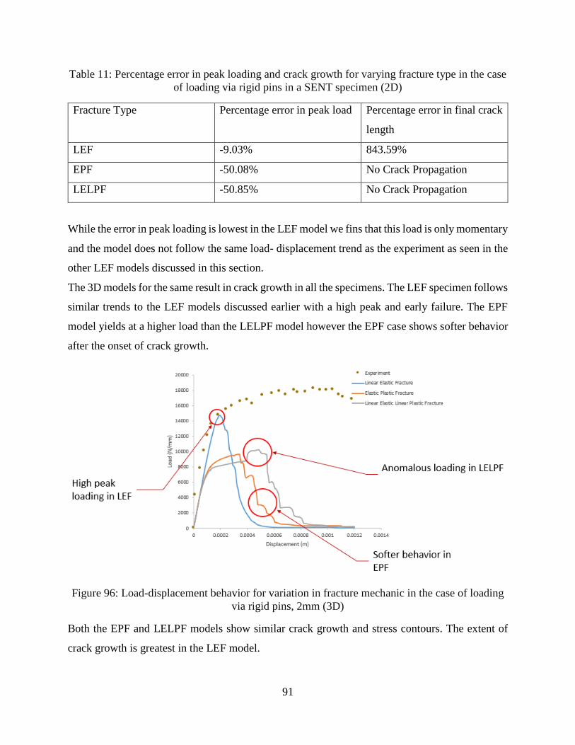
91
Table 11: Percentage error in peak loading and crack growth for varying fracture type in the case
of loading via rigid pins in a SENT specimen (2D)
Fracture Type Percentage error in peak load Percentage error in final crack
length
LEF -9.03% 843.59%
EPF -50.08% No Crack Propagation
LELPF -50.85% No Crack Propagation
While the error in peak loading is lowest in the LEF model we fins that this load is only momentary
and the model does not follow the same load- displacement trend as the experiment as seen in the
other LEF models discussed in this section.
The 3D models for the same result in crack growth in all the specimens. The LEF specimen follows
similar trends to the LEF models discussed earlier with a high peak and early failure. The EPF
model yields at a higher load than the LELPF model however the EPF case shows softer behavior
after the onset of crack growth.
Figure 96: Load-displacement behavior for variation in fracture mechanic in the case of loading
via rigid pins, 2mm (3D)
Both the EPF and LELPF models show similar crack growth and stress contours. The extent of
crack growth is greatest in the LEF model.
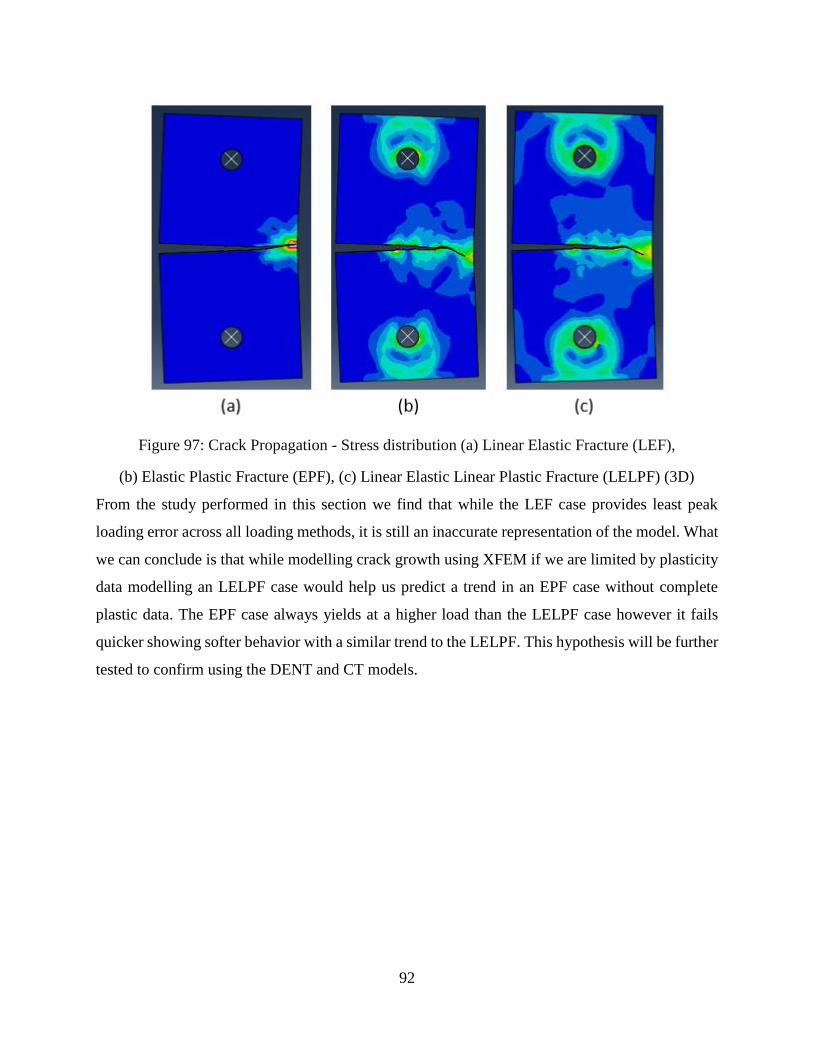
92
Figure 97: Crack Propagation - Stress distribution (a) Linear Elastic Fracture (LEF),
(b) Elastic Plastic Fracture (EPF), (c) Linear Elastic Linear Plastic Fracture (LELPF) (3D)
From the study performed in this section we find that while the LEF case provides least peak
loading error across all loading methods, it is still an inaccurate representation of the model. What
we can conclude is that while modelling crack growth using XFEM if we are limited by plasticity
data modelling an LELPF case would help us predict a trend in an EPF case without complete
plastic data. The EPF case always yields at a higher load than the LELPF case however it fails
quicker showing softer behavior with a similar trend to the LELPF. This hypothesis will be further
tested to confirm using the DENT and CT models.
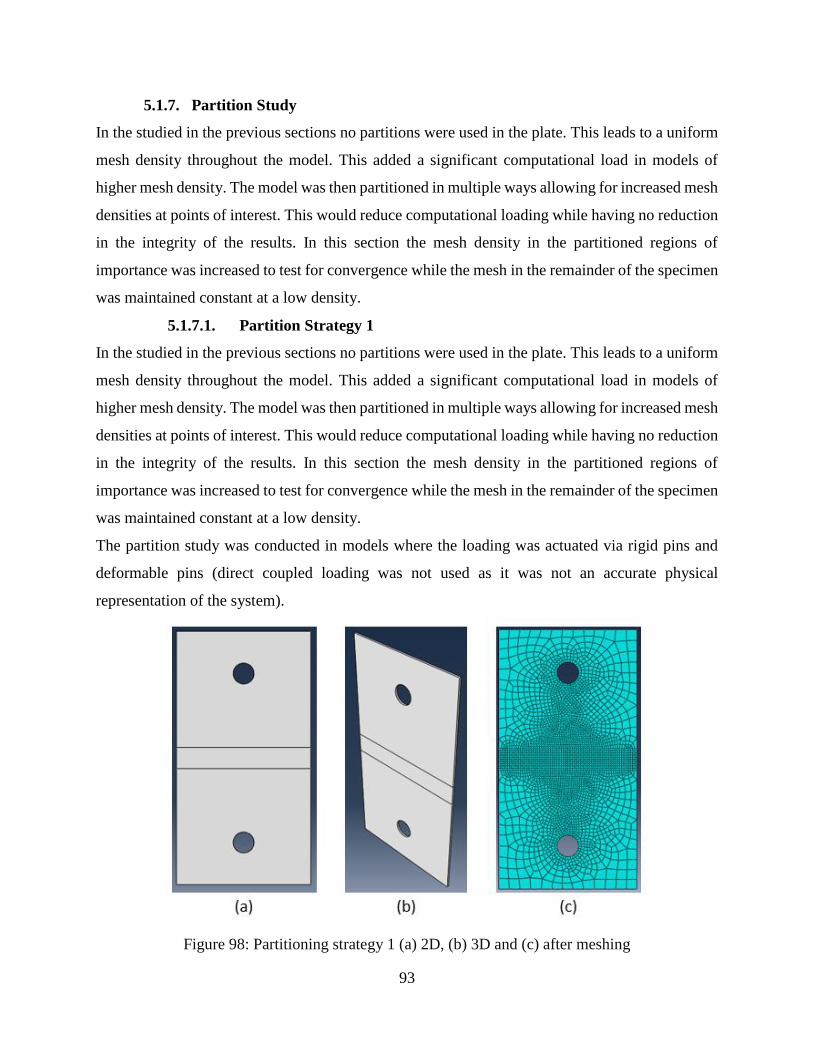
93
5.1.7. Partition Study
In the studied in the previous sections no partitions were used in the plate. This leads to a uniform
mesh density throughout the model. This added a significant computational load in models of
higher mesh density. The model was then partitioned in multiple ways allowing for increased mesh
densities at points of interest. This would reduce computational loading while having no reduction
in the integrity of the results. In this section the mesh density in the partitioned regions of
importance was increased to test for convergence while the mesh in the remainder of the specimen
was maintained constant at a low density.
5.1.7.1. Partition Strategy 1
In the studied in the previous sections no partitions were used in the plate. This leads to a uniform
mesh density throughout the model. This added a significant computational load in models of
higher mesh density. The model was then partitioned in multiple ways allowing for increased mesh
densities at points of interest. This would reduce computational loading while having no reduction
in the integrity of the results. In this section the mesh density in the partitioned regions of
importance was increased to test for convergence while the mesh in the remainder of the specimen
was maintained constant at a low density.
The partition study was conducted in models where the loading was actuated via rigid pins and
deformable pins (direct coupled loading was not used as it was not an accurate physical
representation of the system).
Figure 98: Partitioning strategy 1 (a) 2D, (b) 3D and (c) after meshing
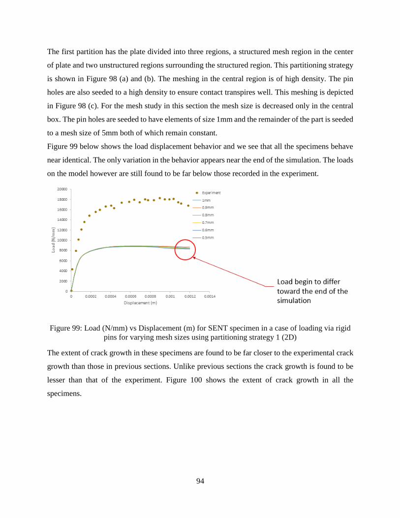
94
The first partition has the plate divided into three regions, a structured mesh region in the center
of plate and two unstructured regions surrounding the structured region. This partitioning strategy
is shown in Figure 98 (a) and (b). The meshing in the central region is of high density. The pin
holes are also seeded to a high density to ensure contact transpires well. This meshing is depicted
in Figure 98 (c). For the mesh study in this section the mesh size is decreased only in the central
box. The pin holes are seeded to have elements of size 1mm and the remainder of the part is seeded
to a mesh size of 5mm both of which remain constant.
Figure 99 below shows the load displacement behavior and we see that all the specimens behave
near identical. The only variation in the behavior appears near the end of the simulation. The loads
on the model however are still found to be far below those recorded in the experiment.
Figure 99: Load (N/mm) vs Displacement (m) for SENT specimen in a case of loading via rigid
pins for varying mesh sizes using partitioning strategy 1 (2D)
The extent of crack growth in these specimens are found to be far closer to the experimental crack
growth than those in previous sections. Unlike previous sections the crack growth is found to be
lesser than that of the experiment. Figure 100 shows the extent of crack growth in all the
specimens.
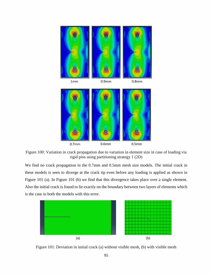
95
Figure 100: Variation in crack propagation due to variation in element size in case of loading via
rigid pins using partitioning strategy 1 (2D)
We find no crack propagation in the 0.7mm and 0.5mm mesh size models. The initial crack in
these models is seen to diverge at the crack tip even before any loading is applied as shown in
Figure 101 (a). In Figure 101 (b) we find that this divergence takes place over a single element.
Also the initial crack is found to lie exactly on the boundary between two layers of elements which
is the case in both the models with this error.
Figure 101: Deviation in initial crack (a) without visible mesh, (b) with visible mesh
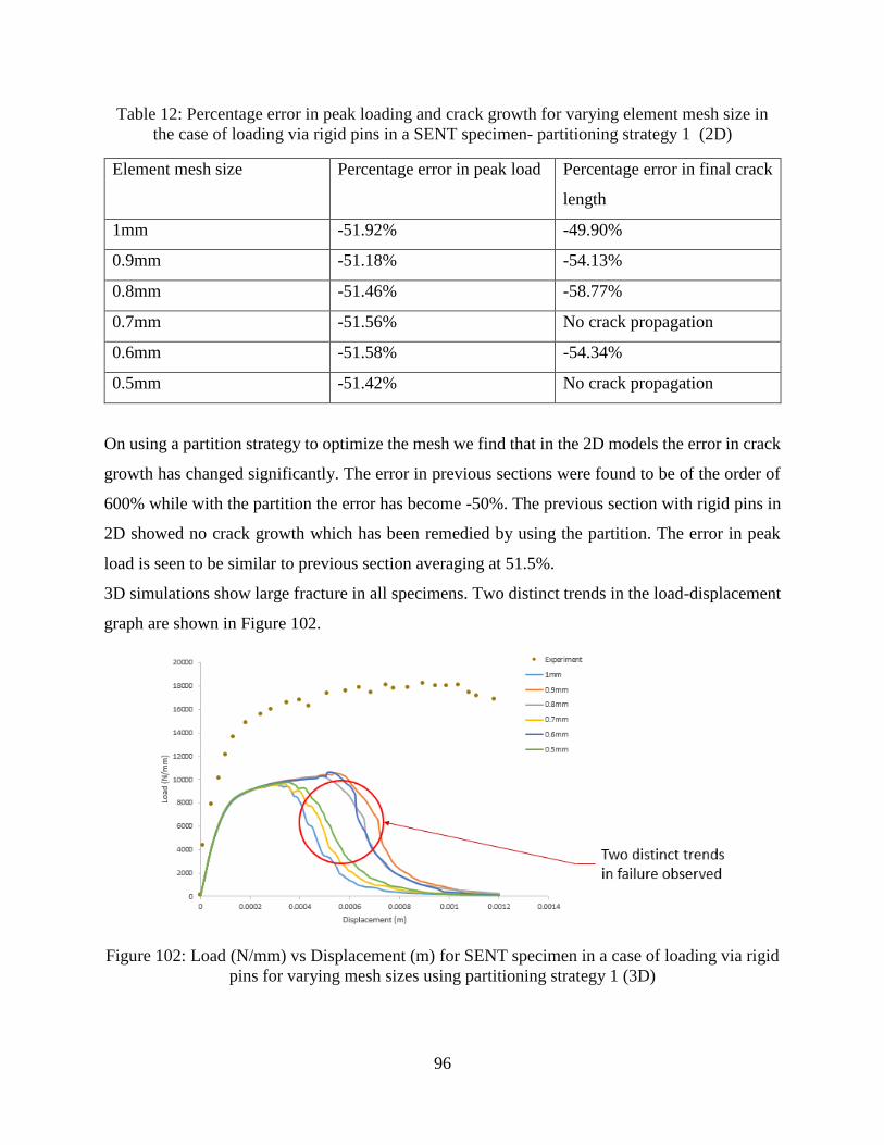
96
Table 12: Percentage error in peak loading and crack growth for varying element mesh size in
the case of loading via rigid pins in a SENT specimen- partitioning strategy 1 (2D)
Element mesh size Percentage error in peak load Percentage error in final crack
length
1mm -51.92% -49.90%
0.9mm -51.18% -54.13%
0.8mm -51.46% -58.77%
0.7mm -51.56% No crack propagation
0.6mm -51.58% -54.34%
0.5mm -51.42% No crack propagation
On using a partition strategy to optimize the mesh we find that in the 2D models the error in crack
growth has changed significantly. The error in previous sections were found to be of the order of
600% while with the partition the error has become -50%. The previous section with rigid pins in
2D showed no crack growth which has been remedied by using the partition. The error in peak
load is seen to be similar to previous section averaging at 51.5%.
3D simulations show large fracture in all specimens. Two distinct trends in the load-displacement
graph are shown in Figure 102.
Figure 102: Load (N/mm) vs Displacement (m) for SENT specimen in a case of loading via rigid
pins for varying mesh sizes using partitioning strategy 1 (3D)
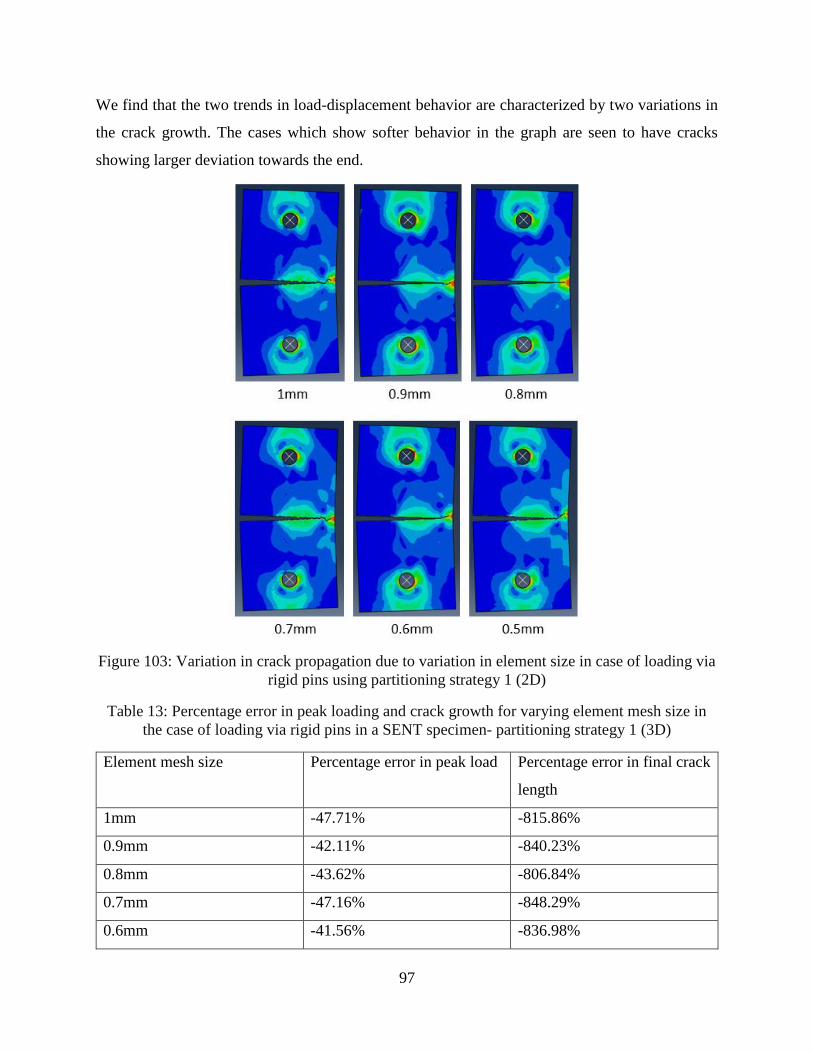
97
We find that the two trends in load-displacement behavior are characterized by two variations in
the crack growth. The cases which show softer behavior in the graph are seen to have cracks
showing larger deviation towards the end.
Figure 103: Variation in crack propagation due to variation in element size in case of loading via
rigid pins using partitioning strategy 1 (2D)
Table 13: Percentage error in peak loading and crack growth for varying element mesh size in
the case of loading via rigid pins in a SENT specimen- partitioning strategy 1 (3D)
Element mesh size Percentage error in peak load Percentage error in final crack
length
1mm -47.71% -815.86%
0.9mm -42.11% -840.23%
0.8mm -43.62% -806.84%
0.7mm -47.16% -848.29%
0.6mm -41.56% -836.98%
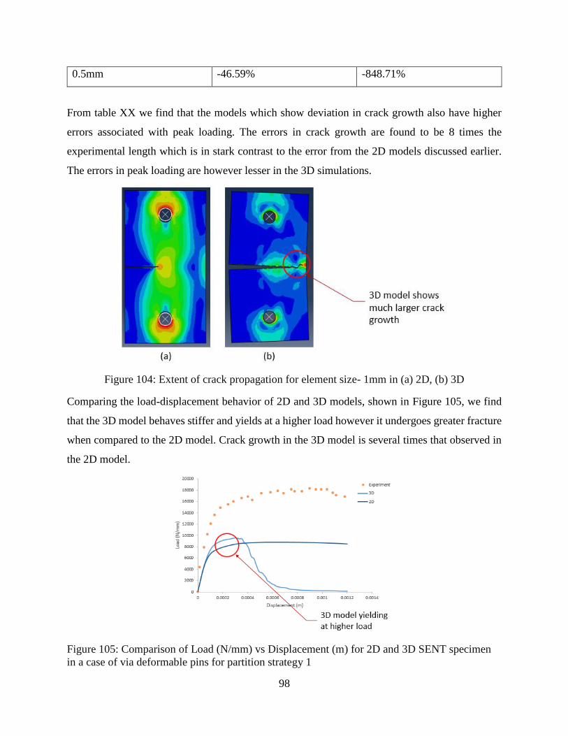
98
0.5mm -46.59% -848.71%
From table XX we find that the models which show deviation in crack growth also have higher
errors associated with peak loading. The errors in crack growth are found to be 8 times the
experimental length which is in stark contrast to the error from the 2D models discussed earlier.
The errors in peak loading are however lesser in the 3D simulations.
Figure 104: Extent of crack propagation for element size- 1mm in (a) 2D, (b) 3D
Comparing the load-displacement behavior of 2D and 3D models, shown in Figure 105, we find
that the 3D model behaves stiffer and yields at a higher load however it undergoes greater fracture
when compared to the 2D model. Crack growth in the 3D model is several times that observed in
the 2D model.
Figure 105: Comparison of Load (N/mm) vs Displacement (m) for 2D and 3D SENT specimen
in a case of via deformable pins for partition strategy 1
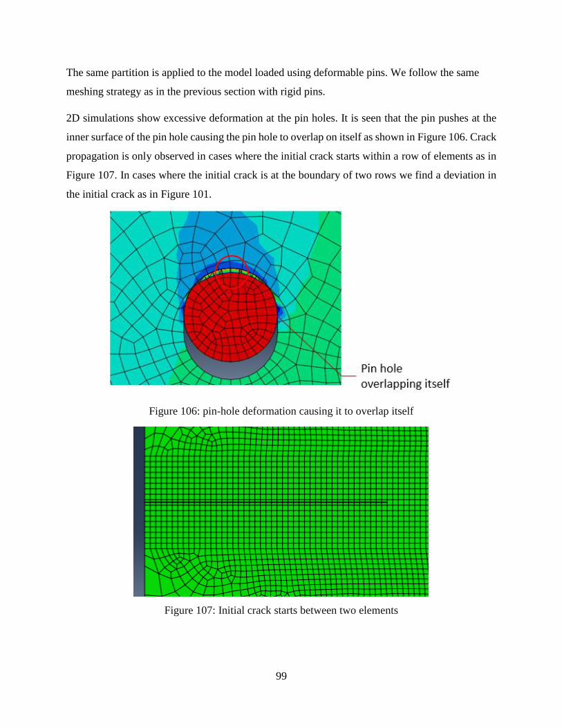
99
The same partition is applied to the model loaded using deformable pins. We follow the same
meshing strategy as in the previous section with rigid pins.
2D simulations show excessive deformation at the pin holes. It is seen that the pin pushes at the
inner surface of the pin hole causing the pin hole to overlap on itself as shown in Figure 106. Crack
propagation is only observed in cases where the initial crack starts within a row of elements as in
Figure 107. In cases where the initial crack is at the boundary of two rows we find a deviation in
the initial crack as in Figure 101.
Figure 106: pin-hole deformation causing it to overlap itself
Figure 107: Initial crack starts between two elements
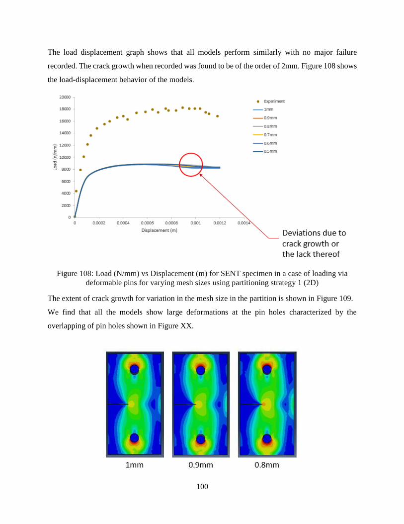
100
The load displacement graph shows that all models perform similarly with no major failure
recorded. The crack growth when recorded was found to be of the order of 2mm. Figure 108 shows
the load-displacement behavior of the models.
Figure 108: Load (N/mm) vs Displacement (m) for SENT specimen in a case of loading via
deformable pins for varying mesh sizes using partitioning strategy 1 (2D)
The extent of crack growth for variation in the mesh size in the partition is shown in Figure 109.
We find that all the models show large deformations at the pin holes characterized by the
overlapping of pin holes shown in Figure XX.
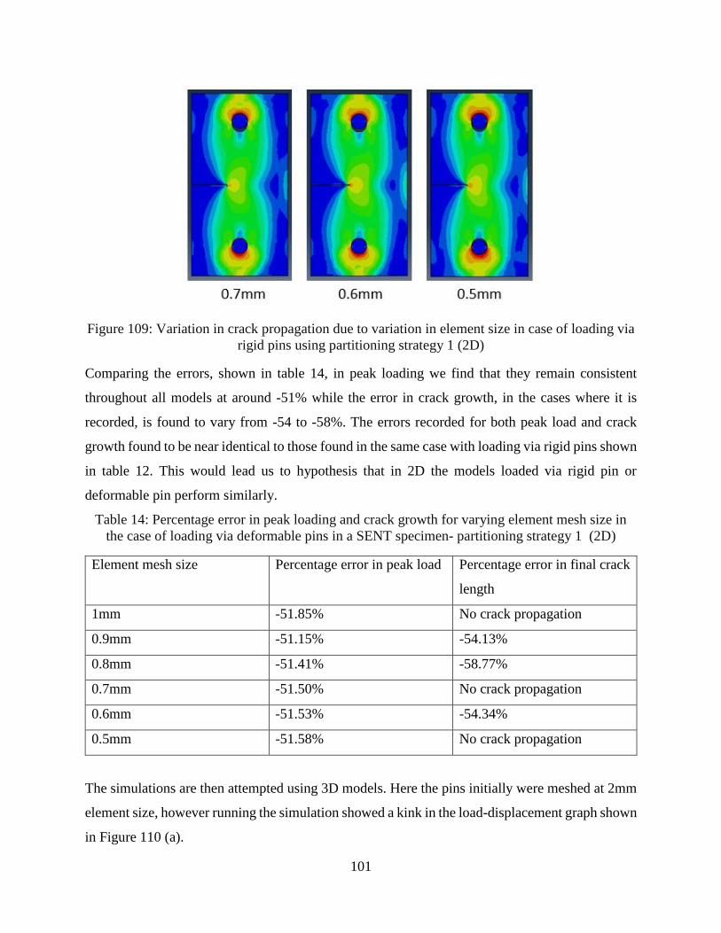
101
Figure 109: Variation in crack propagation due to variation in element size in case of loading via
rigid pins using partitioning strategy 1 (2D)
Comparing the errors, shown in table 14, in peak loading we find that they remain consistent
throughout all models at around -51% while the error in crack growth, in the cases where it is
recorded, is found to vary from -54 to -58%. The errors recorded for both peak load and crack
growth found to be near identical to those found in the same case with loading via rigid pins shown
in table 12. This would lead us to hypothesis that in 2D the models loaded via rigid pin or
deformable pin perform similarly.
Table 14: Percentage error in peak loading and crack growth for varying element mesh size in
the case of loading via deformable pins in a SENT specimen- partitioning strategy 1 (2D)
Element mesh size Percentage error in peak load Percentage error in final crack
length
1mm -51.85% No crack propagation
0.9mm -51.15% -54.13%
0.8mm -51.41% -58.77%
0.7mm -51.50% No crack propagation
0.6mm -51.53% -54.34%
0.5mm -51.58% No crack propagation
The simulations are then attempted using 3D models. Here the pins initially were meshed at 2mm
element size, however running the simulation showed a kink in the load-displacement graph shown
in Figure 110 (a).
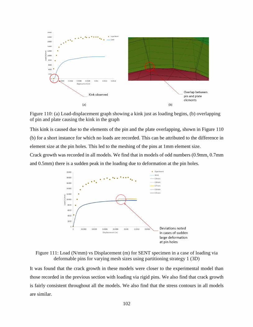
102
Figure 110: (a) Load-displacement graph showing a kink just as loading begins, (b) overlapping
of pin and plate causing the kink in the graph
This kink is caused due to the elements of the pin and the plate overlapping, shown in Figure 110
(b) for a short instance for which no loads are recorded. This can be attributed to the difference in
element size at the pin holes. This led to the meshing of the pins at 1mm element size.
Crack growth was recorded in all models. We find that in models of odd numbers (0.9mm, 0.7mm
and 0.5mm) there is a sudden peak in the loading due to deformation at the pin holes.
Figure 111: Load (N/mm) vs Displacement (m) for SENT specimen in a case of loading via
deformable pins for varying mesh sizes using partitioning strategy 1 (3D)
It was found that the crack growth in these models were closer to the experimental model than
those recorded in the previous section with loading via rigid pins. We also find that crack growth
is fairly consistent throughout all the models. We also find that the stress contours in all models
are similar.
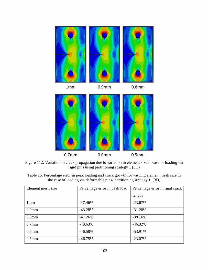
103
Figure 112: Variation in crack propagation due to variation in element size in case of loading via
rigid pins using partitioning strategy 1 (3D)
Table 15: Percentage error in peak loading and crack growth for varying element mesh size in
the case of loading via deformable pins- partitioning strategy 1 (3D)
Element mesh size Percentage error in peak load Percentage error in final crack
length
1mm -47.46% -23.67%
0.9mm -43.28% -31.20%
0.8mm -47.26% -38.16%
0.7mm -43.63% -46.32%
0.6mm -46.58% -53.91%
0.5mm -46.75% -23.07%
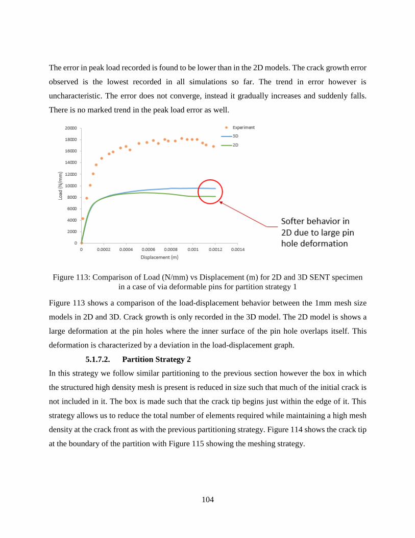
104
The error in peak load recorded is found to be lower than in the 2D models. The crack growth error
observed is the lowest recorded in all simulations so far. The trend in error however is
uncharacteristic. The error does not converge, instead it gradually increases and suddenly falls.
There is no marked trend in the peak load error as well.
Figure 113: Comparison of Load (N/mm) vs Displacement (m) for 2D and 3D SENT specimen
in a case of via deformable pins for partition strategy 1
Figure 113 shows a comparison of the load-displacement behavior between the 1mm mesh size
models in 2D and 3D. Crack growth is only recorded in the 3D model. The 2D model is shows a
large deformation at the pin holes where the inner surface of the pin hole overlaps itself. This
deformation is characterized by a deviation in the load-displacement graph.
5.1.7.2. Partition Strategy 2
In this strategy we follow similar partitioning to the previous section however the box in which
the structured high density mesh is present is reduced in size such that much of the initial crack is
not included in it. The box is made such that the crack tip begins just within the edge of it. This
strategy allows us to reduce the total number of elements required while maintaining a high mesh
density at the crack front as with the previous partitioning strategy. Figure 114 shows the crack tip
at the boundary of the partition with Figure 115 showing the meshing strategy.
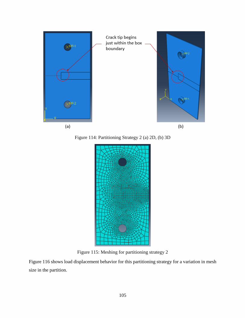
105
Figure 114: Partitioning Strategy 2 (a) 2D, (b) 3D
Figure 115: Meshing for partitioning strategy 2
Figure 116 shows load displacement behavior for this partitioning strategy for a variation in mesh
size in the partition.
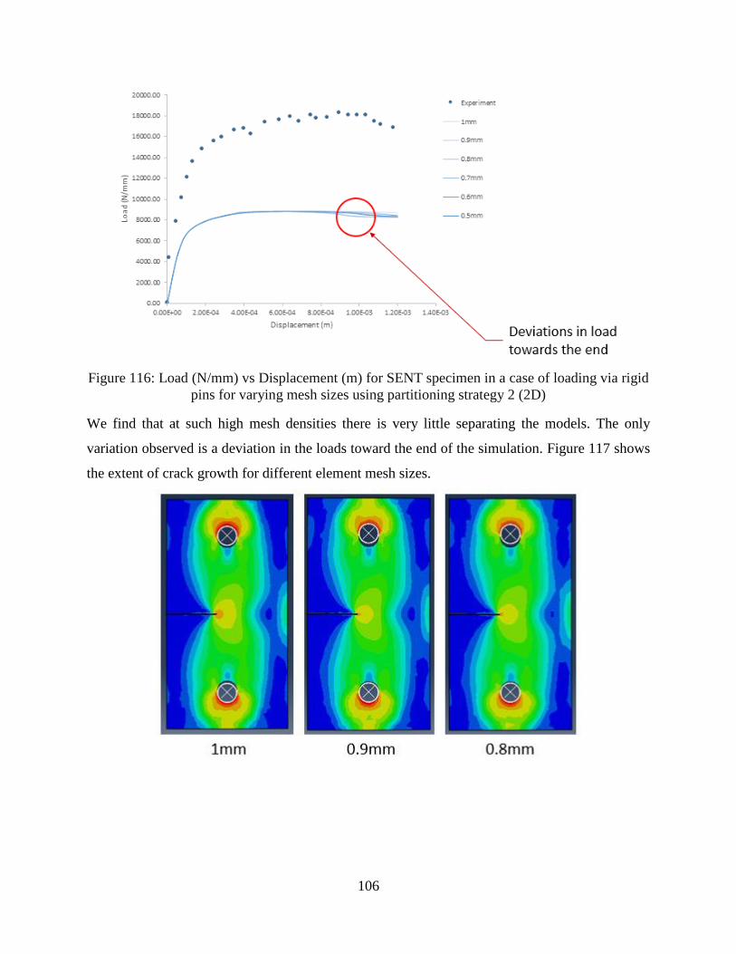
106
Figure 116: Load (N/mm) vs Displacement (m) for SENT specimen in a case of loading via rigid
pins for varying mesh sizes using partitioning strategy 2 (2D)
We find that at such high mesh densities there is very little separating the models. The only
variation observed is a deviation in the loads toward the end of the simulation. Figure 117 shows
the extent of crack growth for different element mesh sizes.
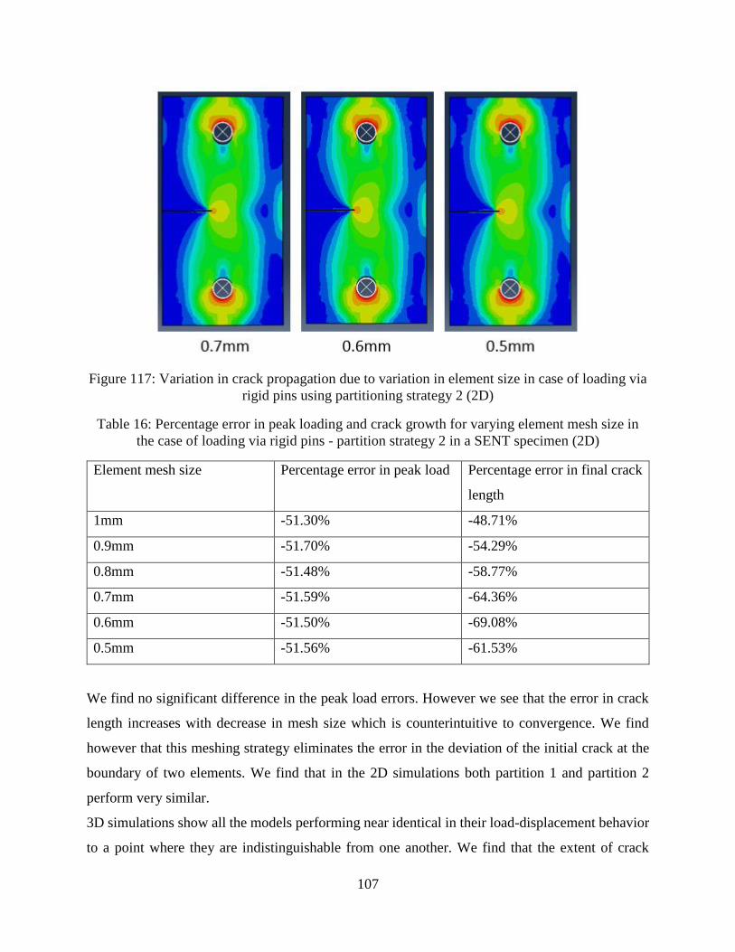
107
Figure 117: Variation in crack propagation due to variation in element size in case of loading via
rigid pins using partitioning strategy 2 (2D)
Table 16: Percentage error in peak loading and crack growth for varying element mesh size in
the case of loading via rigid pins - partition strategy 2 in a SENT specimen (2D)
Element mesh size Percentage error in peak load Percentage error in final crack
length
1mm -51.30% -48.71%
0.9mm -51.70% -54.29%
0.8mm -51.48% -58.77%
0.7mm -51.59% -64.36%
0.6mm -51.50% -69.08%
0.5mm -51.56% -61.53%
We find no significant difference in the peak load errors. However we see that the error in crack
length increases with decrease in mesh size which is counterintuitive to convergence. We find
however that this meshing strategy eliminates the error in the deviation of the initial crack at the
boundary of two elements. We find that in the 2D simulations both partition 1 and partition 2
perform very similar.
3D simulations show all the models performing near identical in their load-displacement behavior
to a point where they are indistinguishable from one another. We find that the extent of crack
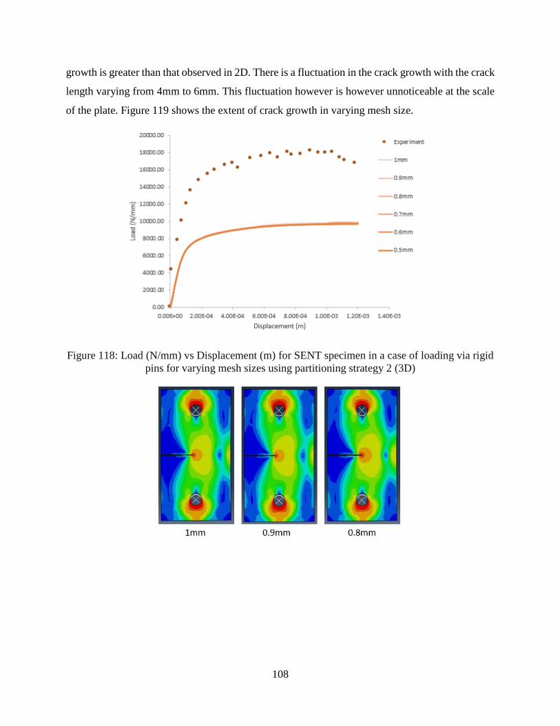
108
growth is greater than that observed in 2D. There is a fluctuation in the crack growth with the crack
length varying from 4mm to 6mm. This fluctuation however is however unnoticeable at the scale
of the plate. Figure 119 shows the extent of crack growth in varying mesh size.
Figure 118: Load (N/mm) vs Displacement (m) for SENT specimen in a case of loading via rigid
pins for varying mesh sizes using partitioning strategy 2 (3D)
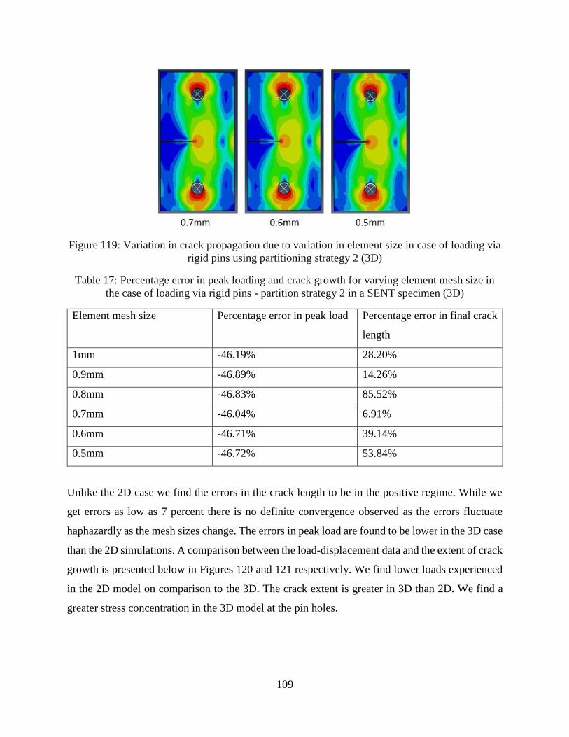
109
Figure 119: Variation in crack propagation due to variation in element size in case of loading via
rigid pins using partitioning strategy 2 (3D)
Table 17: Percentage error in peak loading and crack growth for varying element mesh size in
the case of loading via rigid pins - partition strategy 2 in a SENT specimen (3D)
Element mesh size Percentage error in peak load Percentage error in final crack
length
1mm -46.19% 28.20%
0.9mm -46.89% 14.26%
0.8mm -46.83% 85.52%
0.7mm -46.04% 6.91%
0.6mm -46.71% 39.14%
0.5mm -46.72% 53.84%
Unlike the 2D case we find the errors in the crack length to be in the positive regime. While we
get errors as low as 7 percent there is no definite convergence observed as the errors fluctuate
haphazardly as the mesh sizes change. The errors in peak load are found to be lower in the 3D case
than the 2D simulations. A comparison between the load-displacement data and the extent of crack
growth is presented below in Figures 120 and 121 respectively. We find lower loads experienced
in the 2D model on comparison to the 3D. The crack extent is greater in 3D than 2D. We find a
greater stress concentration in the 3D model at the pin holes.
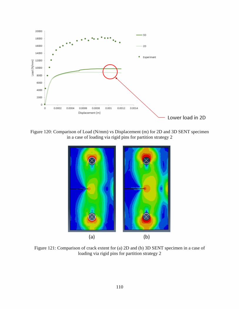
110
Figure 120: Comparison of Load (N/mm) vs Displacement (m) for 2D and 3D SENT specimen
in a case of loading via rigid pins for partition strategy 2
Figure 121: Comparison of crack extent for (a) 2D and (b) 3D SENT specimen in a case of
loading via rigid pins for partition strategy 2
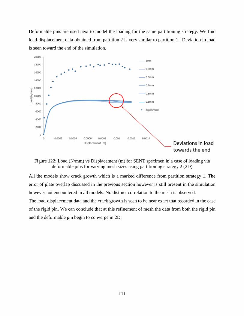
111
Deformable pins are used next to model the loading for the same partitioning strategy. We find
load-displacement data obtained from partition 2 is very similar to partition 1. Deviation in load
is seen toward the end of the simulation.
Figure 122: Load (N/mm) vs Displacement (m) for SENT specimen in a case of loading via
deformable pins for varying mesh sizes using partitioning strategy 2 (2D)
All the models show crack growth which is a marked difference from partition strategy 1. The
error of plate overlap discussed in the previous section however is still present in the simulation
however not encountered in all models. No distinct correlation to the mesh is observed.
The load-displacement data and the crack growth is seen to be near exact that recorded in the case
of the rigid pin. We can conclude that at this refinement of mesh the data from both the rigid pin
and the deformable pin begin to converge in 2D.
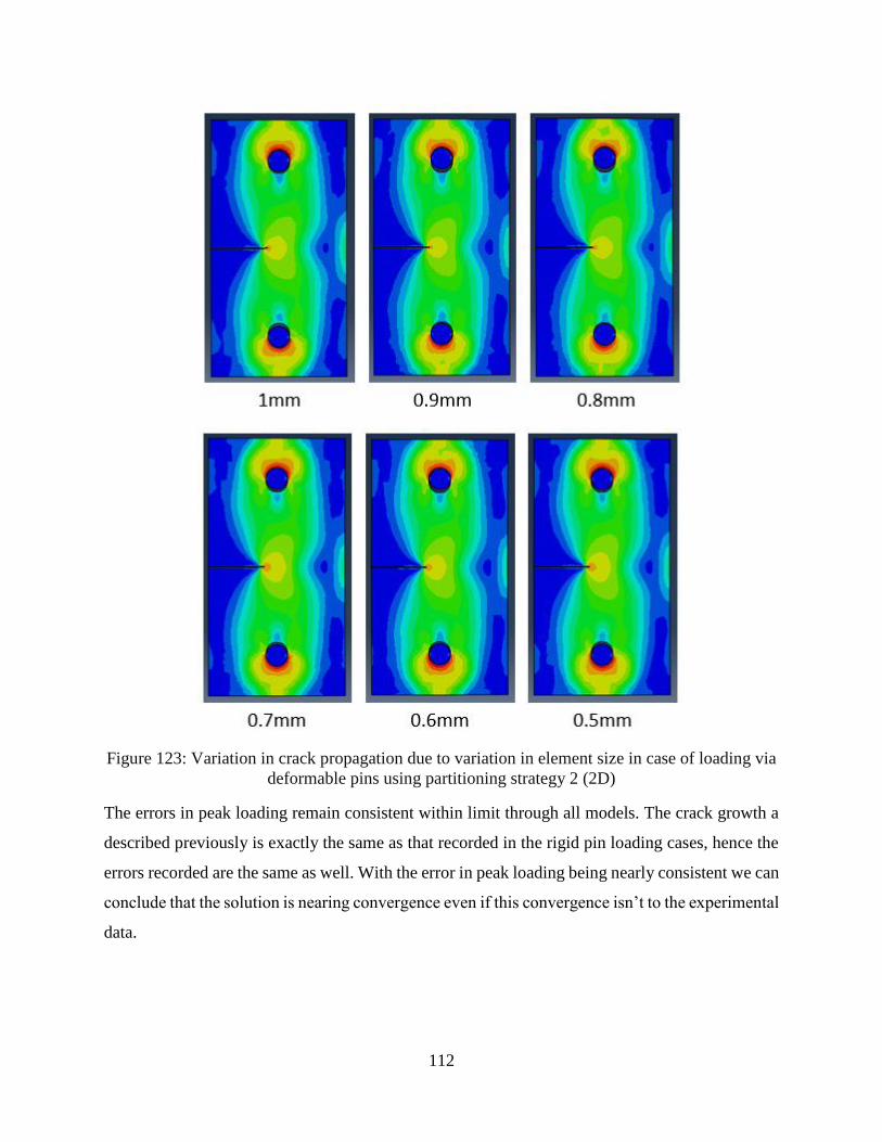
112
Figure 123: Variation in crack propagation due to variation in element size in case of loading via
deformable pins using partitioning strategy 2 (2D)
The errors in peak loading remain consistent within limit through all models. The crack growth a
described previously is exactly the same as that recorded in the rigid pin loading cases, hence the
errors recorded are the same as well. With the error in peak loading being nearly consistent we can
conclude that the solution is nearing convergence even if this convergence isn’t to the experimental
data.
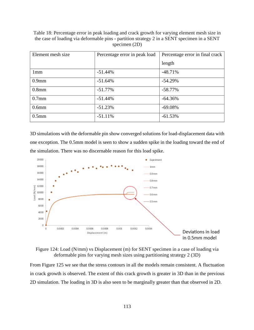
113
Table 18: Percentage error in peak loading and crack growth for varying element mesh size in
the case of loading via deformable pins - partition strategy 2 in a SENT specimen in a SENT
specimen (2D)
Element mesh size Percentage error in peak load Percentage error in final crack
length
1mm -51.44% -48.71%
0.9mm -51.64% -54.29%
0.8mm -51.77% -58.77%
0.7mm -51.44% -64.36%
0.6mm -51.23% -69.08%
0.5mm -51.11% -61.53%
3D simulations with the deformable pin show converged solutions for load-displacement data with
one exception. The 0.5mm model is seen to show a sudden spike in the loading toward the end of
the simulation. There was no discernable reason for this load spike.
Figure 124: Load (N/mm) vs Displacement (m) for SENT specimen in a case of loading via
deformable pins for varying mesh sizes using partitioning strategy 2 (3D)
From Figure 125 we see that the stress contours in all the models remain consistent. A fluctuation
in crack growth is observed. The extent of this crack growth is greater in 3D than in the previous
2D simulation. The loading in 3D is also seen to be marginally greater than that observed in 2D.
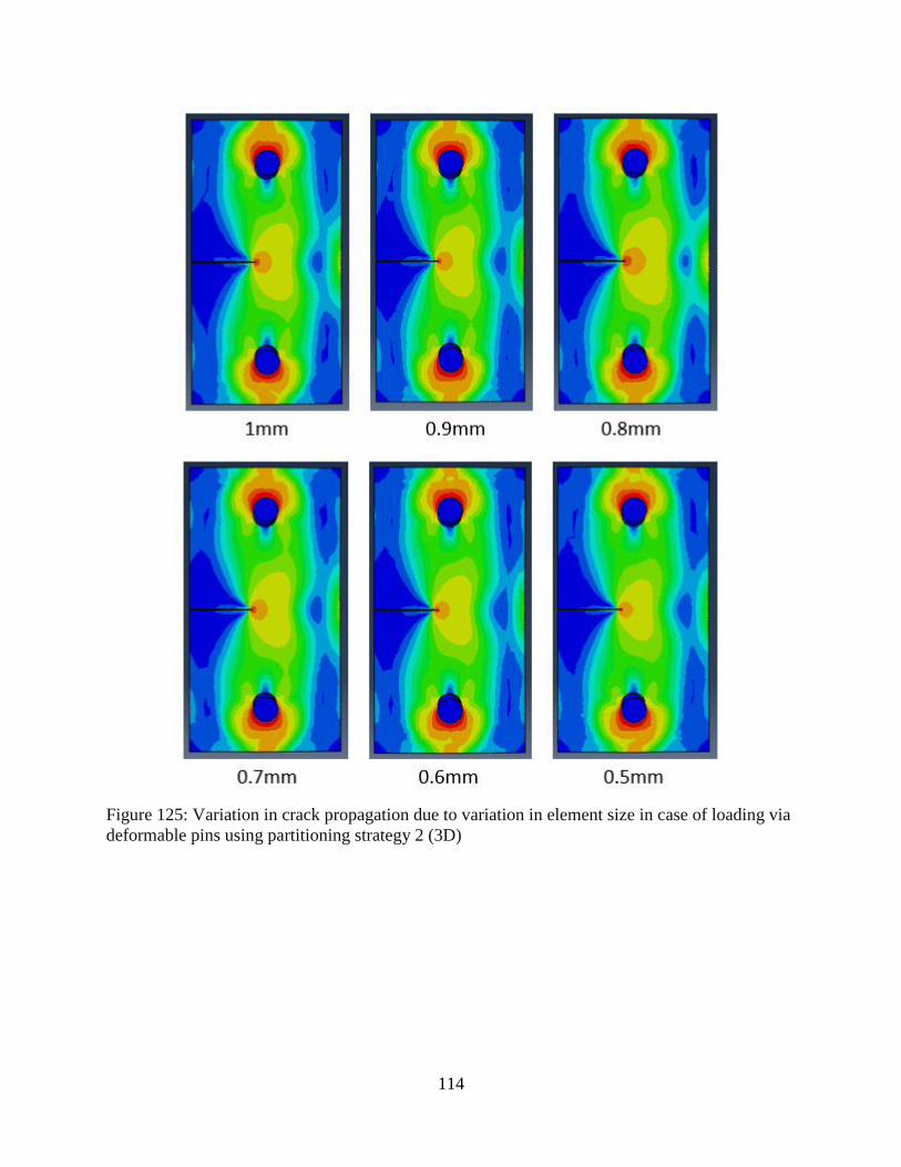
114
Figure 125: Variation in crack propagation due to variation in element size in case of loading via
deformable pins using partitioning strategy 2 (3D)
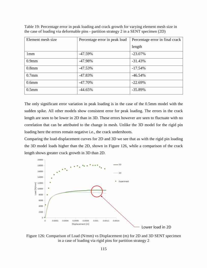
115
Table 19: Percentage error in peak loading and crack growth for varying element mesh size in
the case of loading via deformable pins - partition strategy 2 in a SENT specimen (2D)
Element mesh size Percentage error in peak load Percentage error in final crack
length
1mm -47.59% -23.07%
0.9mm -47.98% -31.43%
0.8mm -47.53% -17.54%
0.7mm -47.83% -46.54%
0.6mm -47.70% -22.69%
0.5mm -44.65% -35.89%
The only significant error variation in peak loading is in the case of the 0.5mm model with the
sudden spike. All other models show consistent error for peak loading. The errors in the crack
length are seen to be lower in 2D than in 3D. These errors however are seen to fluctuate with no
correlation that can be attributed to the change in mesh. Unlike the 3D model for the rigid pin
loading here the errors remain negative i.e., the crack undershoots.
Comparing the load-displacement curves for 2D and 3D we see that as with the rigid pin loading
the 3D model loads higher than the 2D, shown in Figure 126, while a comparison of the crack
length shows greater crack growth in 3D than 2D.
Figure 126: Comparison of Load (N/mm) vs Displacement (m) for 2D and 3D SENT specimen
in a case of loading via rigid pins for partition strategy 2
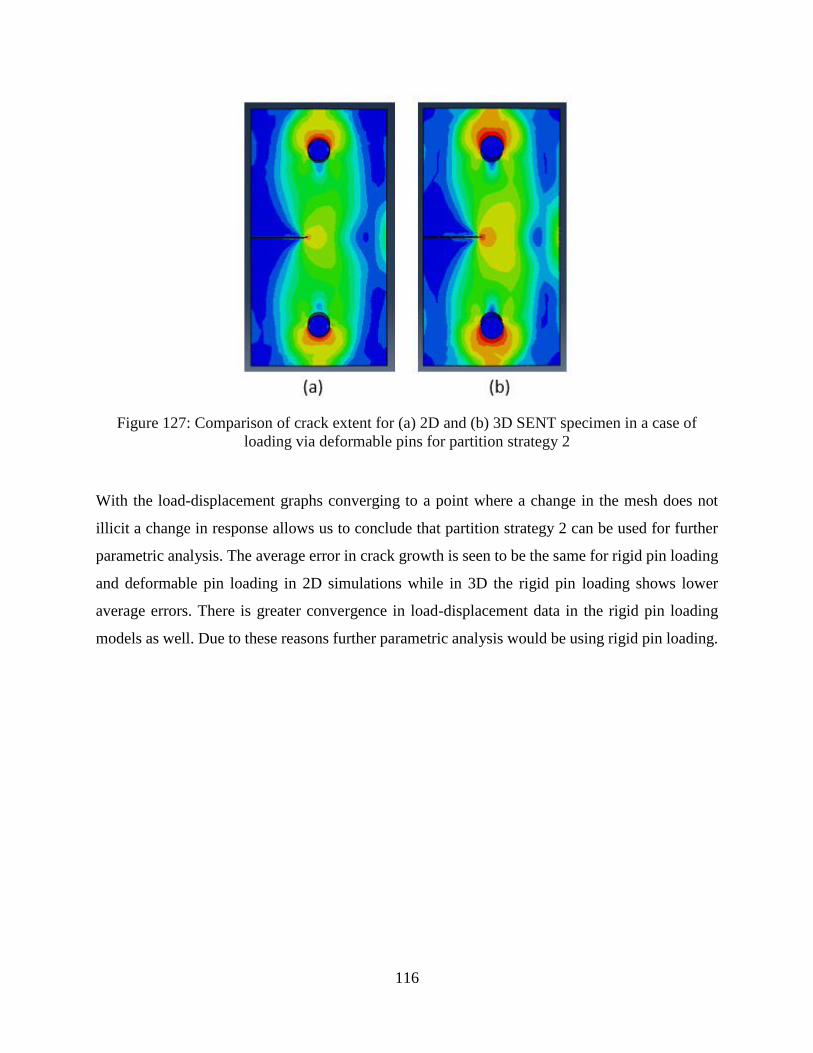
116
Figure 127: Comparison of crack extent for (a) 2D and (b) 3D SENT specimen in a case of
loading via deformable pins for partition strategy 2
With the load-displacement graphs converging to a point where a change in the mesh does not
illicit a change in response allows us to conclude that partition strategy 2 can be used for further
parametric analysis. The average error in crack growth is seen to be the same for rigid pin loading
and deformable pin loading in 2D simulations while in 3D the rigid pin loading shows lower
average errors. There is greater convergence in load-displacement data in the rigid pin loading
models as well. Due to these reasons further parametric analysis would be using rigid pin loading.
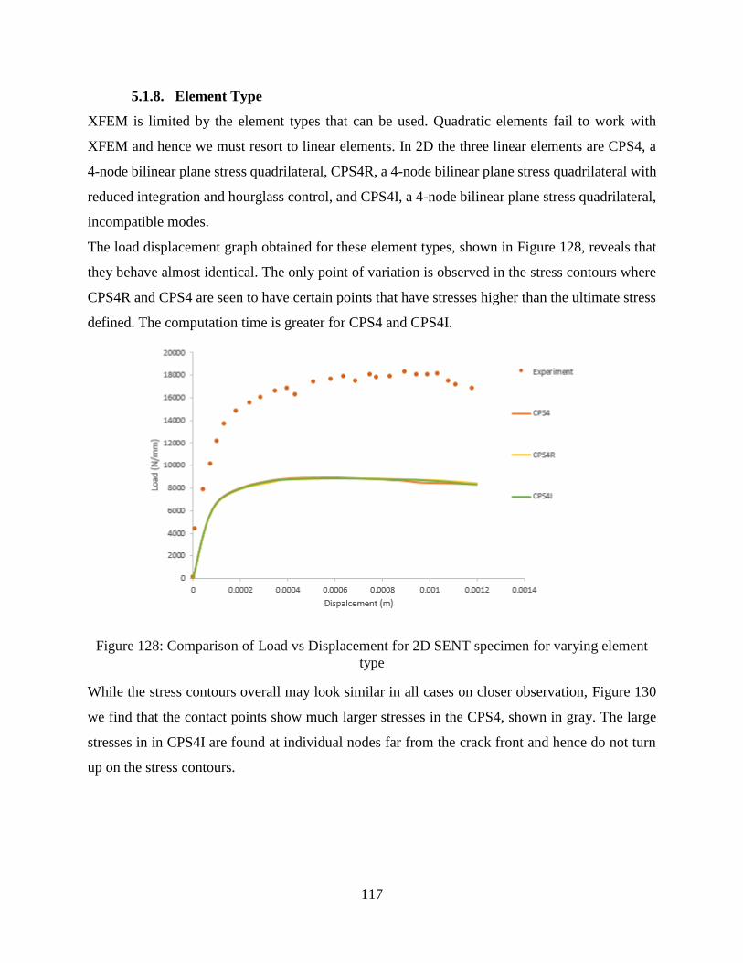
117
5.1.8. Element Type
XFEM is limited by the element types that can be used. Quadratic elements fail to work with
XFEM and hence we must resort to linear elements. In 2D the three linear elements are CPS4, a
4-node bilinear plane stress quadrilateral, CPS4R, a 4-node bilinear plane stress quadrilateral with
reduced integration and hourglass control, and CPS4I, a 4-node bilinear plane stress quadrilateral,
incompatible modes.
The load displacement graph obtained for these element types, shown in Figure 128, reveals that
they behave almost identical. The only point of variation is observed in the stress contours where
CPS4R and CPS4 are seen to have certain points that have stresses higher than the ultimate stress
defined. The computation time is greater for CPS4 and CPS4I.
Figure 128: Comparison of Load vs Displacement for 2D SENT specimen for varying element
type
While the stress contours overall may look similar in all cases on closer observation, Figure 130
we find that the contact points show much larger stresses in the CPS4, shown in gray. The large
stresses in in CPS4I are found at individual nodes far from the crack front and hence do not turn
up on the stress contours.
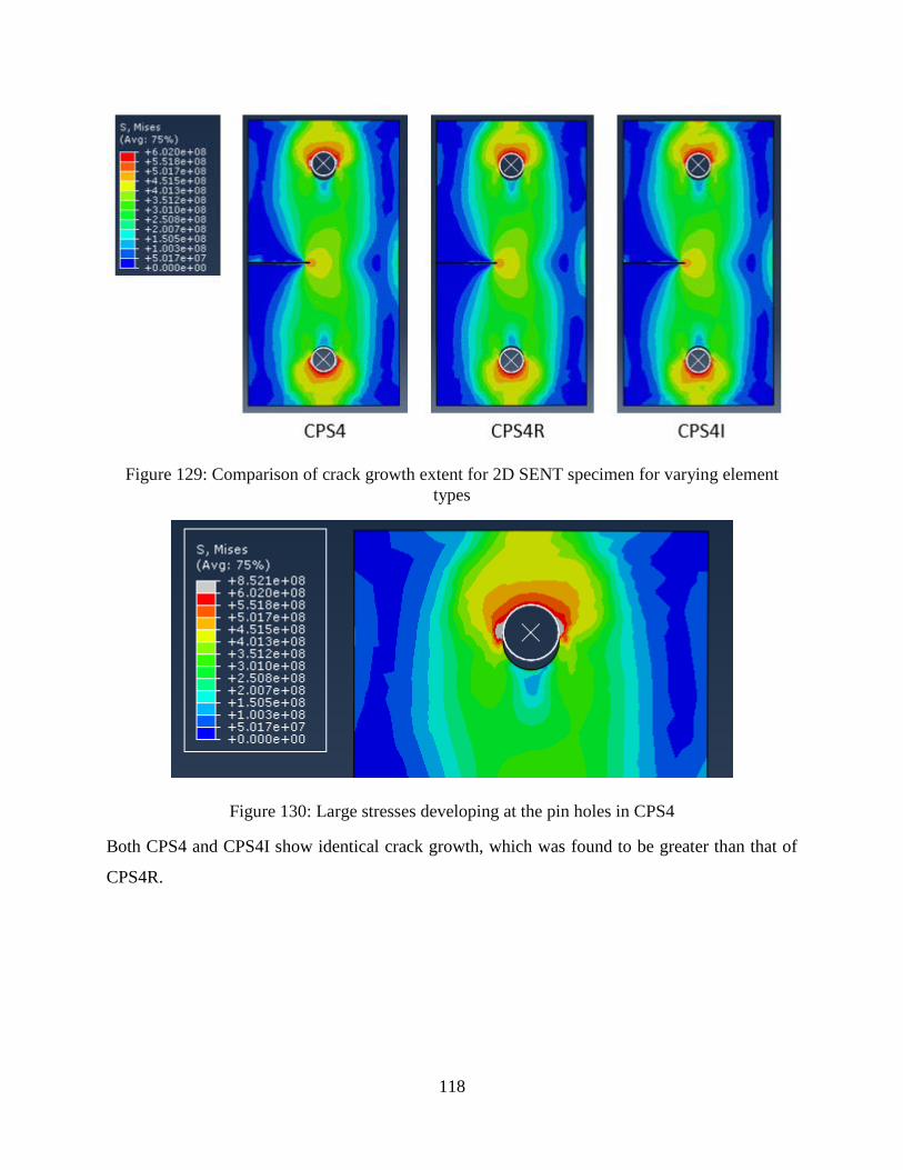
118
Figure 129: Comparison of crack growth extent for 2D SENT specimen for varying element
types
Figure 130: Large stresses developing at the pin holes in CPS4
Both CPS4 and CPS4I show identical crack growth, which was found to be greater than that of
CPS4R.
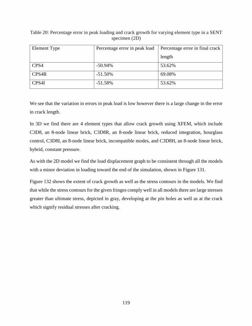
119
Table 20: Percentage error in peak loading and crack growth for varying element type in a SENT
specimen (2D)
Element Type Percentage error in peak load Percentage error in final crack
length
CPS4 -50.94% 53.62%
CPS4R -51.50% 69.08%
CPS4I -51.58% 53.62%
We see that the variation in errors in peak load is low however there is a large change in the error
in crack length.
In 3D we find there are 4 element types that allow crack growth using XFEM, which include
C3D8, an 8-node linear brick, C3D8R, an 8-node linear brick, reduced integration, hourglass
control, C3D8I, an 8-node linear brick, incompatible modes, and C3D8H, an 8-node linear brick,
hybrid, constant pressure.
As with the 2D model we find the load displacement graph to be consistent through all the models
with a minor deviation in loading toward the end of the simulation, shown in Figure 131.
Figure 132 shows the extent of crack growth as well as the stress contours in the models. We find
that while the stress contours for the given fringes comply well in all models there are large stresses
greater than ultimate stress, depicted in gray, developing at the pin holes as well as at the crack
which signify residual stresses after cracking.
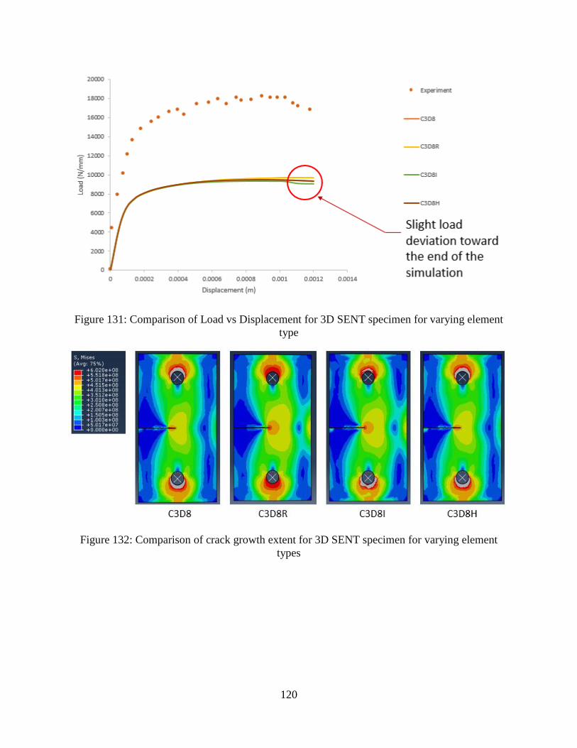
120
Figure 131: Comparison of Load vs Displacement for 3D SENT specimen for varying element
type
Figure 132: Comparison of crack growth extent for 3D SENT specimen for varying element
types
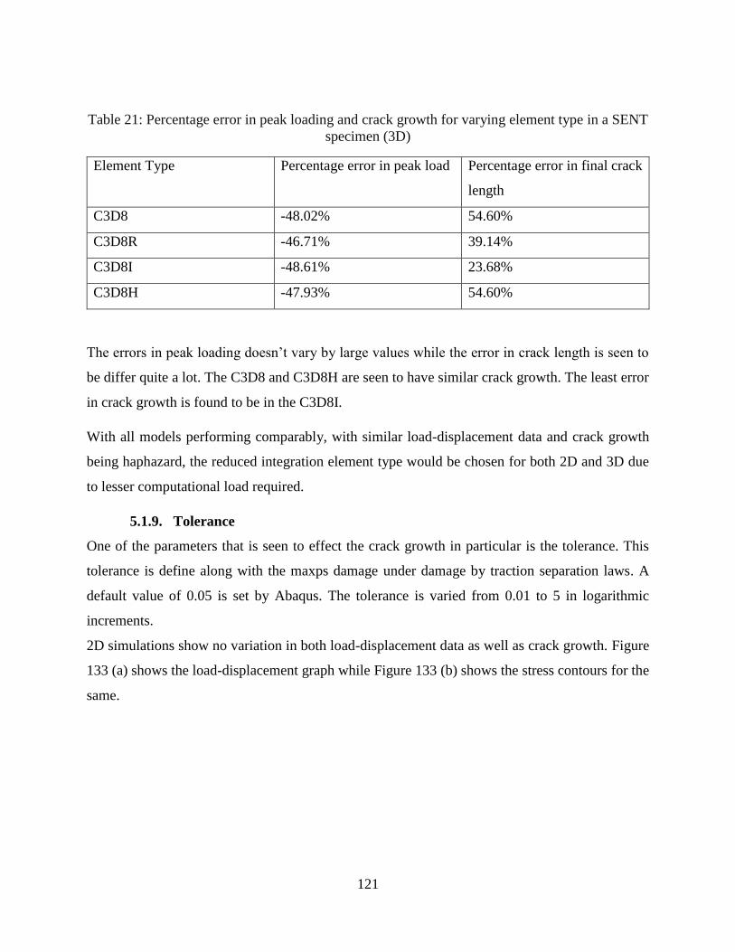
121
Table 21: Percentage error in peak loading and crack growth for varying element type in a SENT
specimen (3D)
Element Type Percentage error in peak load Percentage error in final crack
length
C3D8 -48.02% 54.60%
C3D8R -46.71% 39.14%
C3D8I -48.61% 23.68%
C3D8H -47.93% 54.60%
The errors in peak loading doesn’t vary by large values while the error in crack length is seen to
be differ quite a lot. The C3D8 and C3D8H are seen to have similar crack growth. The least error
in crack growth is found to be in the C3D8I.
With all models performing comparably, with similar load-displacement data and crack growth
being haphazard, the reduced integration element type would be chosen for both 2D and 3D due
to lesser computational load required.
5.1.9. Tolerance
One of the parameters that is seen to effect the crack growth in particular is the tolerance. This
tolerance is define along with the maxps damage under damage by traction separation laws. A
default value of 0.05 is set by Abaqus. The tolerance is varied from 0.01 to 5 in logarithmic
increments.
2D simulations show no variation in both load-displacement data as well as crack growth. Figure
133 (a) shows the load-displacement graph while Figure 133 (b) shows the stress contours for the
same.
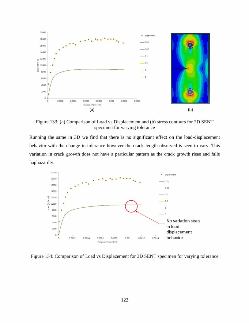
122
Figure 133: (a) Comparison of Load vs Displacement and (b) stress contours for 2D SENT
specimen for varying tolerance
Running the same in 3D we find that there is no significant effect on the load-displacement
behavior with the change in tolerance however the crack length observed is seen to vary. This
variation in crack growth does not have a particular pattern as the crack growth rises and falls
haphazardly.
Figure 134: Comparison of Load vs Displacement for 3D SENT specimen for varying tolerance
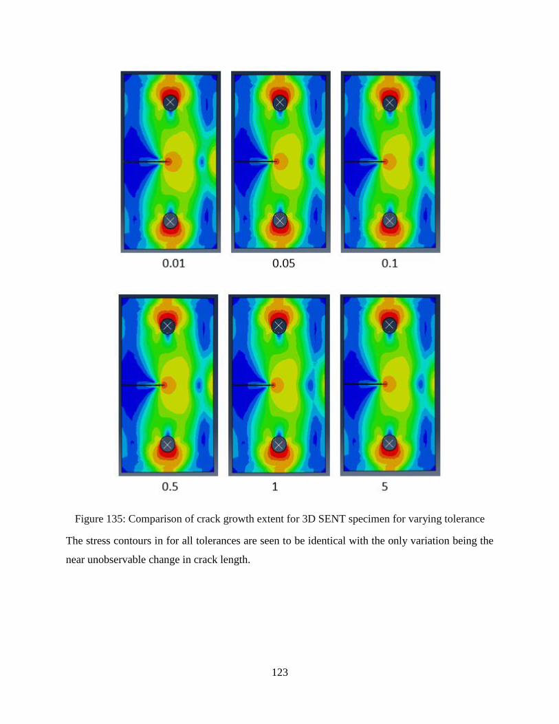
123
Figure 135: Comparison of crack growth extent for 3D SENT specimen for varying tolerance
The stress contours in for all tolerances are seen to be identical with the only variation being the
near unobservable change in crack length.
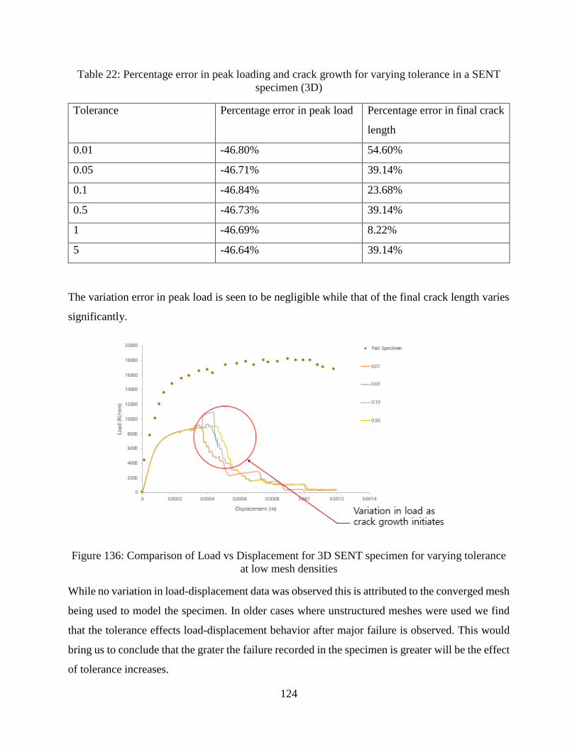
124
Table 22: Percentage error in peak loading and crack growth for varying tolerance in a SENT
specimen (3D)
Tolerance Percentage error in peak load Percentage error in final crack
length
0.01 -46.80% 54.60%
0.05 -46.71% 39.14%
0.1 -46.84% 23.68%
0.5 -46.73% 39.14%
1 -46.69% 8.22%
5 -46.64% 39.14%
The variation error in peak load is seen to be negligible while that of the final crack length varies
significantly.
Figure 136: Comparison of Load vs Displacement for 3D SENT specimen for varying tolerance
at low mesh densities
While no variation in load-displacement data was observed this is attributed to the converged mesh
being used to model the specimen. In older cases where unstructured meshes were used we find
that the tolerance effects load-displacement behavior after major failure is observed. This would
bring us to conclude that the grater the failure recorded in the specimen is greater will be the effect
of tolerance increases.
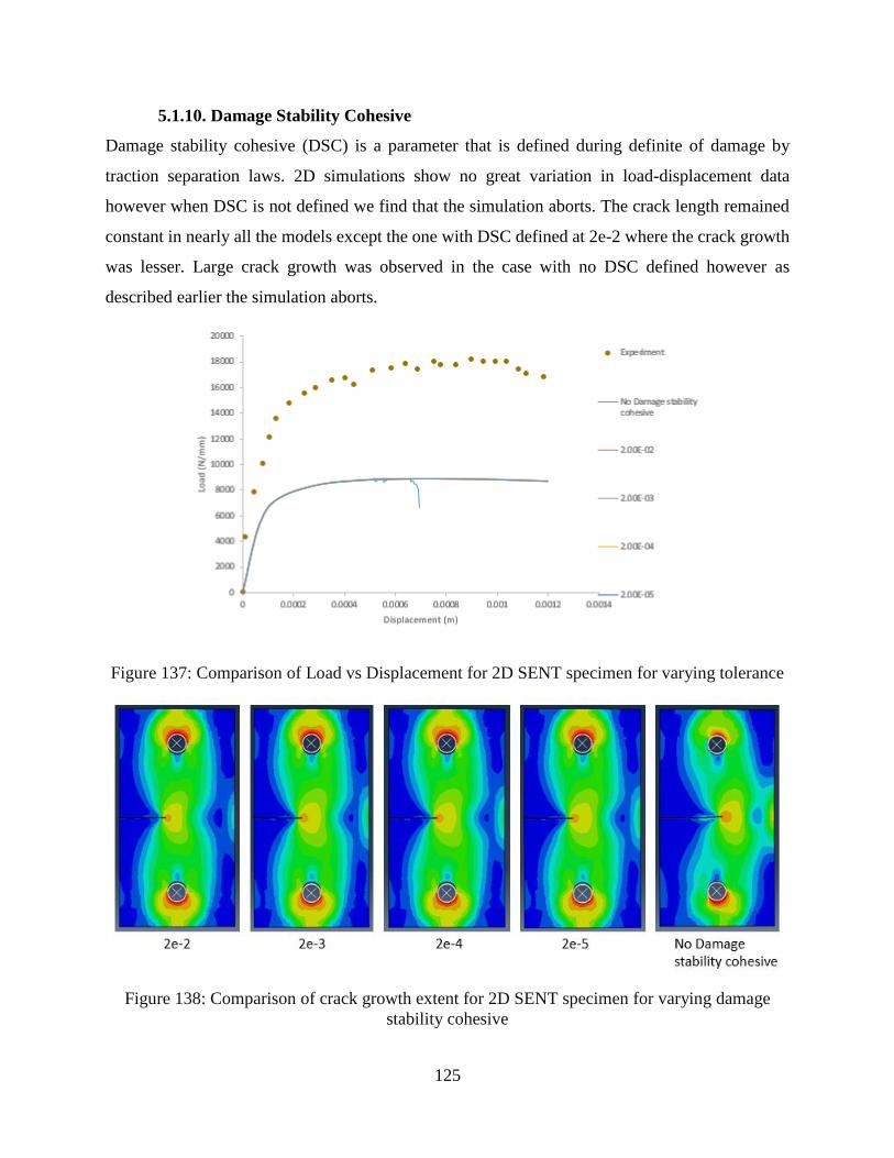
125
5.1.10. Damage Stability Cohesive
Damage stability cohesive (DSC) is a parameter that is defined during definite of damage by
traction separation laws. 2D simulations show no great variation in load-displacement data
however when DSC is not defined we find that the simulation aborts. The crack length remained
constant in nearly all the models except the one with DSC defined at 2e-2 where the crack growth
was lesser. Large crack growth was observed in the case with no DSC defined however as
described earlier the simulation aborts.
Figure 137: Comparison of Load vs Displacement for 2D SENT specimen for varying tolerance
Figure 138: Comparison of crack growth extent for 2D SENT specimen for varying damage
stability cohesive
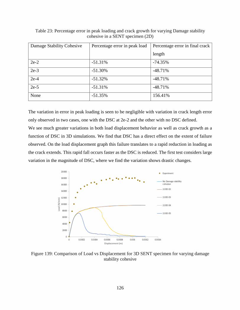
126
Table 23: Percentage error in peak loading and crack growth for varying Damage stability
cohesive in a SENT specimen (2D)
Damage Stability Cohesive Percentage error in peak load Percentage error in final crack
length
2e-2 -51.31% -74.35%
2e-3 -51.30% -48.71%
2e-4 -51.32% -48.71%
2e-5 -51.31% -48.71%
None -51.35% 156.41%
The variation in error in peak loading is seen to be negligible with variation in crack length error
only observed in two cases, one with the DSC at 2e-2 and the other with no DSC defined.
We see much greater variations in both load displacement behavior as well as crack growth as a
function of DSC in 3D simulations. We find that DSC has a direct effect on the extent of failure
observed. On the load displacement graph this failure translates to a rapid reduction in loading as
the crack extends. This rapid fall occurs faster as the DSC is reduced. The first test considers large
variation in the magnitude of DSC, where we find the variation shows drastic changes.
Figure 139: Comparison of Load vs Displacement for 3D SENT specimen for varying damage
stability cohesive
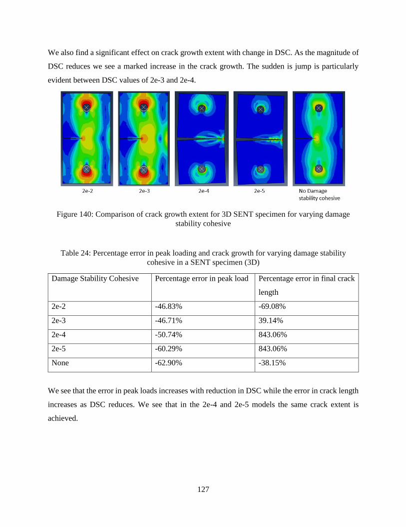
127
We also find a significant effect on crack growth extent with change in DSC. As the magnitude of
DSC reduces we see a marked increase in the crack growth. The sudden is jump is particularly
evident between DSC values of 2e-3 and 2e-4.
Figure 140: Comparison of crack growth extent for 3D SENT specimen for varying damage
stability cohesive
Table 24: Percentage error in peak loading and crack growth for varying damage stability
cohesive in a SENT specimen (3D)
Damage Stability Cohesive Percentage error in peak load Percentage error in final crack
length
2e-2 -46.83% -69.08%
2e-3 -46.71% 39.14%
2e-4 -50.74% 843.06%
2e-5 -60.29% 843.06%
None -62.90% -38.15%
We see that the error in peak loads increases with reduction in DSC while the error in crack length
increases as DSC reduces. We see that in the 2e-4 and 2e-5 models the same crack extent is
achieved.
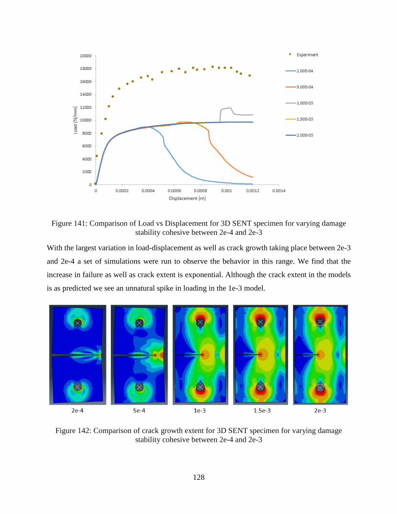
128
Figure 141: Comparison of Load vs Displacement for 3D SENT specimen for varying damage
stability cohesive between 2e-4 and 2e-3
With the largest variation in load-displacement as well as crack growth taking place between 2e-3
and 2e-4 a set of simulations were run to observe the behavior in this range. We find that the
increase in failure as well as crack extent is exponential. Although the crack extent in the models
is as predicted we see an unnatural spike in loading in the 1e-3 model.
Figure 142: Comparison of crack growth extent for 3D SENT specimen for varying damage
stability cohesive between 2e-4 and 2e-3
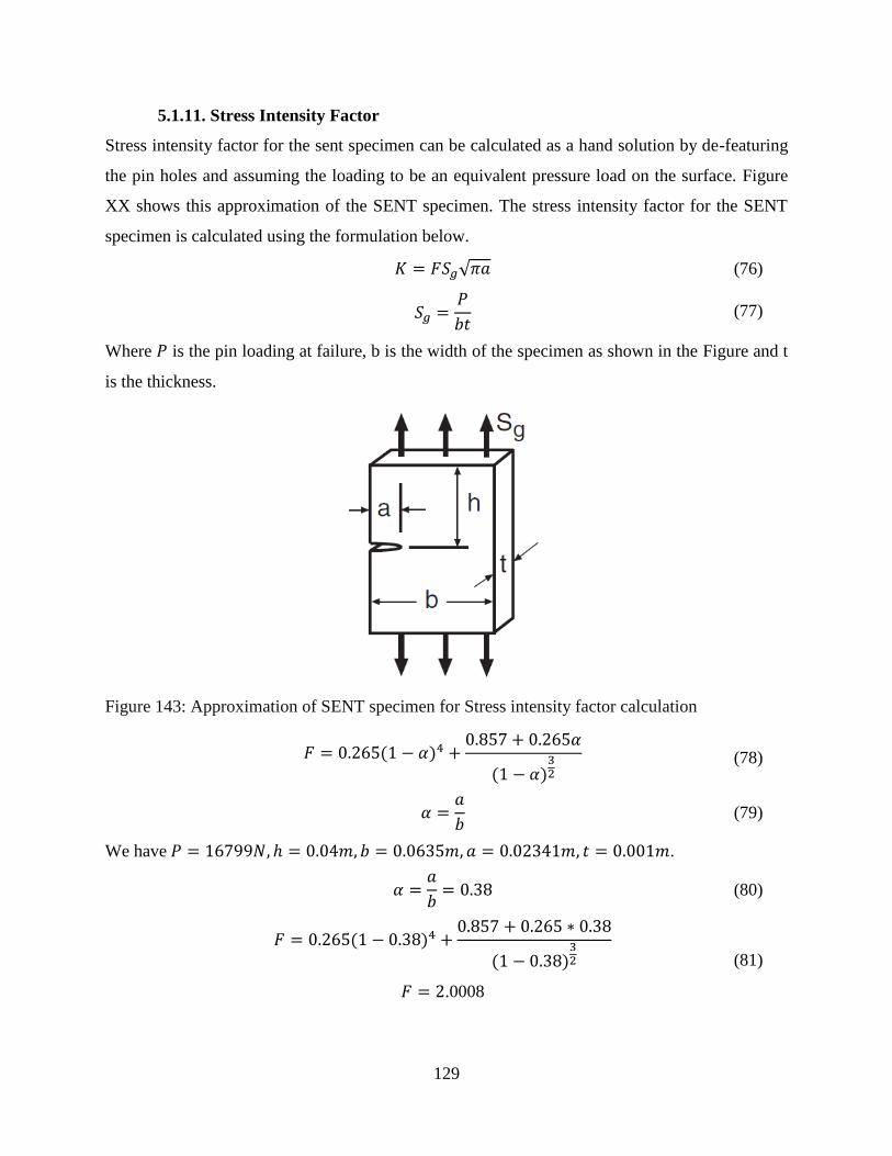
129
5.1.11. Stress Intensity Factor
Stress intensity factor for the sent specimen can be calculated as a hand solution by de-featuring
the pin holes and assuming the loading to be an equivalent pressure load on the surface. Figure
XX shows this approximation of the SENT specimen. The stress intensity factor for the SENT
specimen is calculated using the formulation below.
𝐾 = 𝐹𝑆𝑔√𝜋𝑎 (76)
𝑆𝑔 =𝑃
𝑏𝑡 (77)
Where 𝑃 is the pin loading at failure, b is the width of the specimen as shown in the Figure and t
is the thickness.
Figure 143: Approximation of SENT specimen for Stress intensity factor calculation
𝐹 = 0.265(1 − 𝛼)4 +0.857 + 0.265𝛼
(1 − 𝛼)32
(78)
𝛼 =𝑎
𝑏 (79)
We have 𝑃 = 16799𝑁, ℎ = 0.04𝑚, 𝑏 = 0.0635𝑚, 𝑎 = 0.02341𝑚, 𝑡 = 0.001𝑚.
𝛼 =𝑎
𝑏= 0.38 (80)
𝐹 = 0.265(1 − 0.38)4 +0.857 + 0.265 ∗ 0.38
(1 − 0.38)32
𝐹 = 2.0008
(81)

130
𝐾 = 2.0008 ∗
16799
0.0635 ∗ 0.001√𝜋 ∗ 0.02413
𝐾 = 1.4567 𝑒8 𝑀𝑃𝑎√𝑚
(82)
Stress intensity factor is obtained in using XFEM in Abaqus by assuming the crack to be a
stationary crack and requesting a history output for stress intensity factor. From the requested
history output we obtain K to be 1.4607 𝑒8 𝑀𝑃𝑎√𝑚 which is at a 0.3% error.
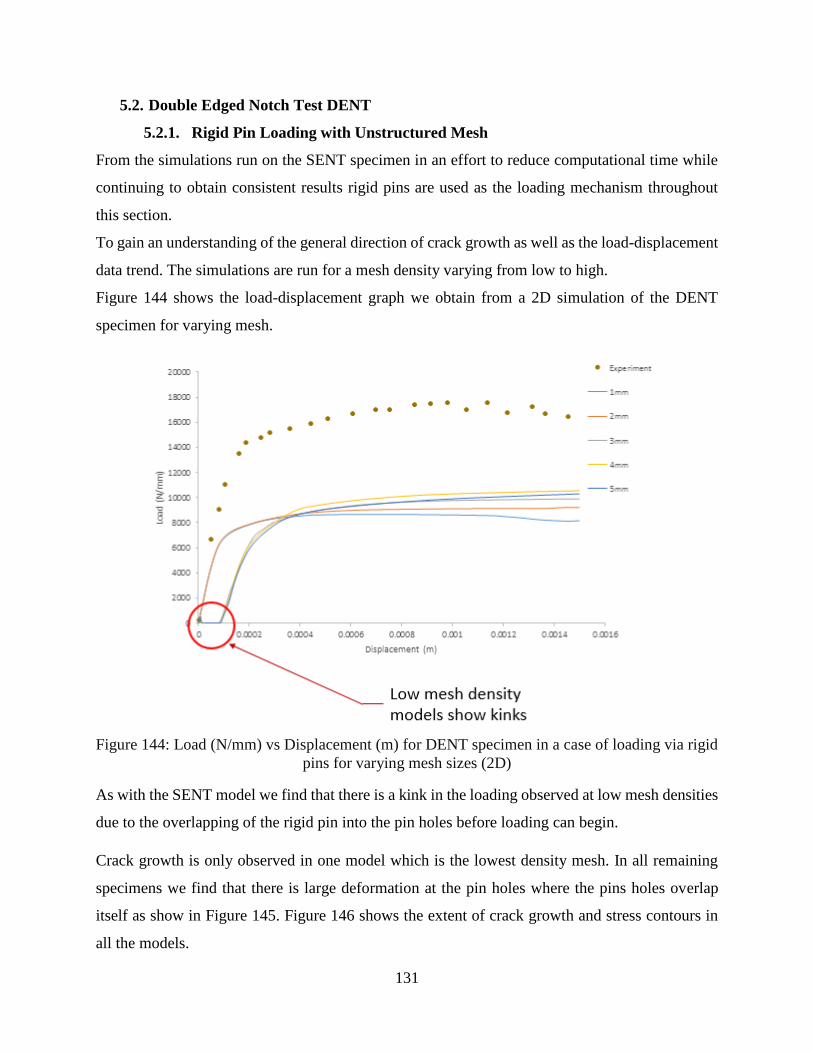
131
5.2. Double Edged Notch Test DENT
5.2.1. Rigid Pin Loading with Unstructured Mesh
From the simulations run on the SENT specimen in an effort to reduce computational time while
continuing to obtain consistent results rigid pins are used as the loading mechanism throughout
this section.
To gain an understanding of the general direction of crack growth as well as the load-displacement
data trend. The simulations are run for a mesh density varying from low to high.
Figure 144 shows the load-displacement graph we obtain from a 2D simulation of the DENT
specimen for varying mesh.
Figure 144: Load (N/mm) vs Displacement (m) for DENT specimen in a case of loading via rigid
pins for varying mesh sizes (2D)
As with the SENT model we find that there is a kink in the loading observed at low mesh densities
due to the overlapping of the rigid pin into the pin holes before loading can begin.
Crack growth is only observed in one model which is the lowest density mesh. In all remaining
specimens we find that there is large deformation at the pin holes where the pins holes overlap
itself as show in Figure 145. Figure 146 shows the extent of crack growth and stress contours in
all the models.
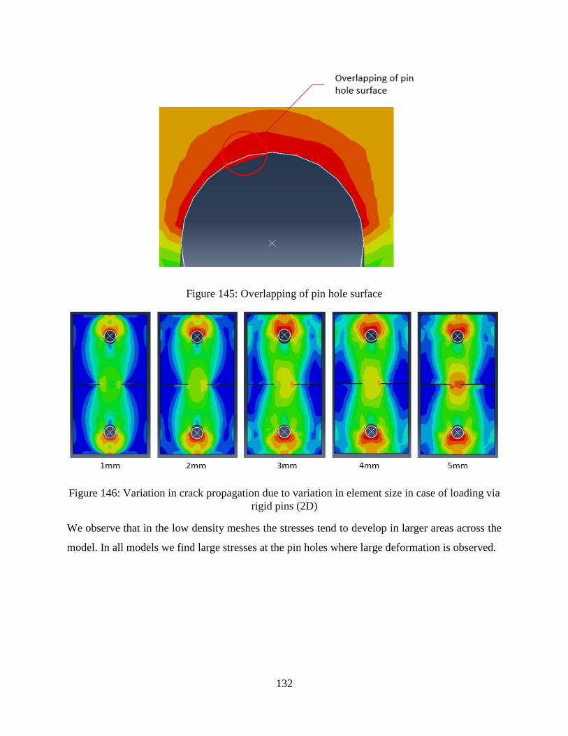
132
Figure 145: Overlapping of pin hole surface
Figure 146: Variation in crack propagation due to variation in element size in case of loading via
rigid pins (2D)
We observe that in the low density meshes the stresses tend to develop in larger areas across the
model. In all models we find large stresses at the pin holes where large deformation is observed.
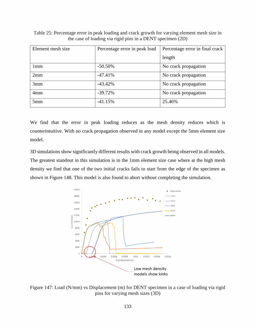
133
Table 25: Percentage error in peak loading and crack growth for varying element mesh size in
the case of loading via rigid pins in a DENT specimen (2D)
Element mesh size Percentage error in peak load Percentage error in final crack
length
1mm -50.50% No crack propagation
2mm -47.41% No crack propagation
3mm -43.42% No crack propagation
4mm -39.72% No crack propagation
5mm -41.15% 25.46%
We find that the error in peak loading reduces as the mesh density reduces which is
counterintuitive. With no crack propagation observed in any model except the 5mm element size
model.
3D simulations show significantly different results with crack growth being observed in all models.
The greatest standout in this simulation is in the 1mm element size case where at the high mesh
density we find that one of the two initial cracks fails to start from the edge of the specimen as
shown in Figure 148. This model is also found to abort without completing the simulation.
Figure 147: Load (N/mm) vs Displacement (m) for DENT specimen in a case of loading via rigid
pins for varying mesh sizes (3D)
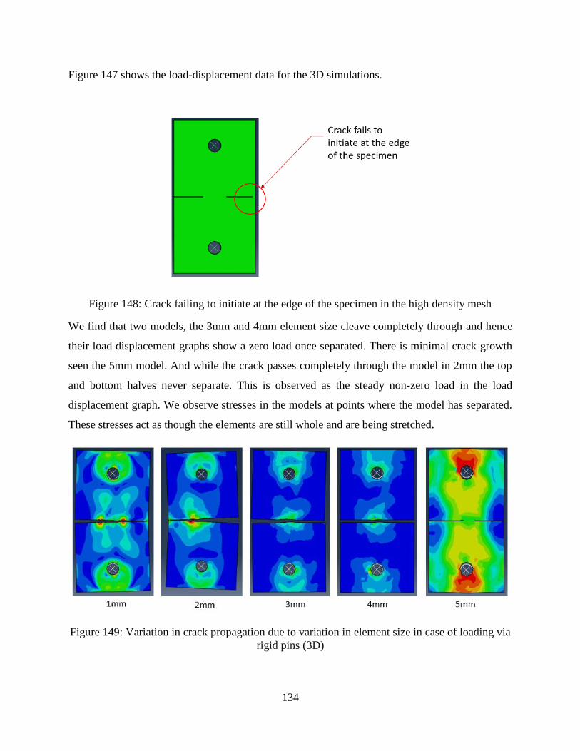
134
Figure 147 shows the load-displacement data for the 3D simulations.
Figure 148: Crack failing to initiate at the edge of the specimen in the high density mesh
We find that two models, the 3mm and 4mm element size cleave completely through and hence
their load displacement graphs show a zero load once separated. There is minimal crack growth
seen the 5mm model. And while the crack passes completely through the model in 2mm the top
and bottom halves never separate. This is observed as the steady non-zero load in the load
displacement graph. We observe stresses in the models at points where the model has separated.
These stresses act as though the elements are still whole and are being stretched.
Figure 149: Variation in crack propagation due to variation in element size in case of loading via
rigid pins (3D)
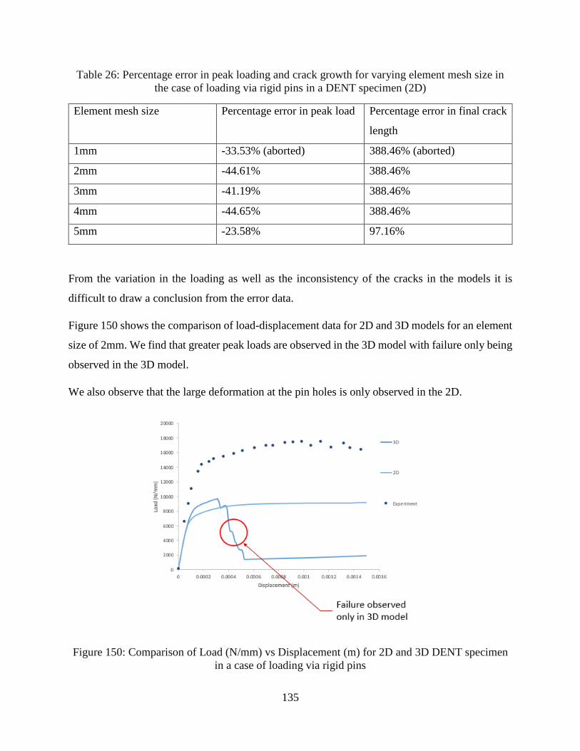
135
Table 26: Percentage error in peak loading and crack growth for varying element mesh size in
the case of loading via rigid pins in a DENT specimen (2D)
Element mesh size Percentage error in peak load Percentage error in final crack
length
1mm -33.53% (aborted) 388.46% (aborted)
2mm -44.61% 388.46%
3mm -41.19% 388.46%
4mm -44.65% 388.46%
5mm -23.58% 97.16%
From the variation in the loading as well as the inconsistency of the cracks in the models it is
difficult to draw a conclusion from the error data.
Figure 150 shows the comparison of load-displacement data for 2D and 3D models for an element
size of 2mm. We find that greater peak loads are observed in the 3D model with failure only being
observed in the 3D model.
We also observe that the large deformation at the pin holes is only observed in the 2D.
Figure 150: Comparison of Load (N/mm) vs Displacement (m) for 2D and 3D DENT specimen
in a case of loading via rigid pins
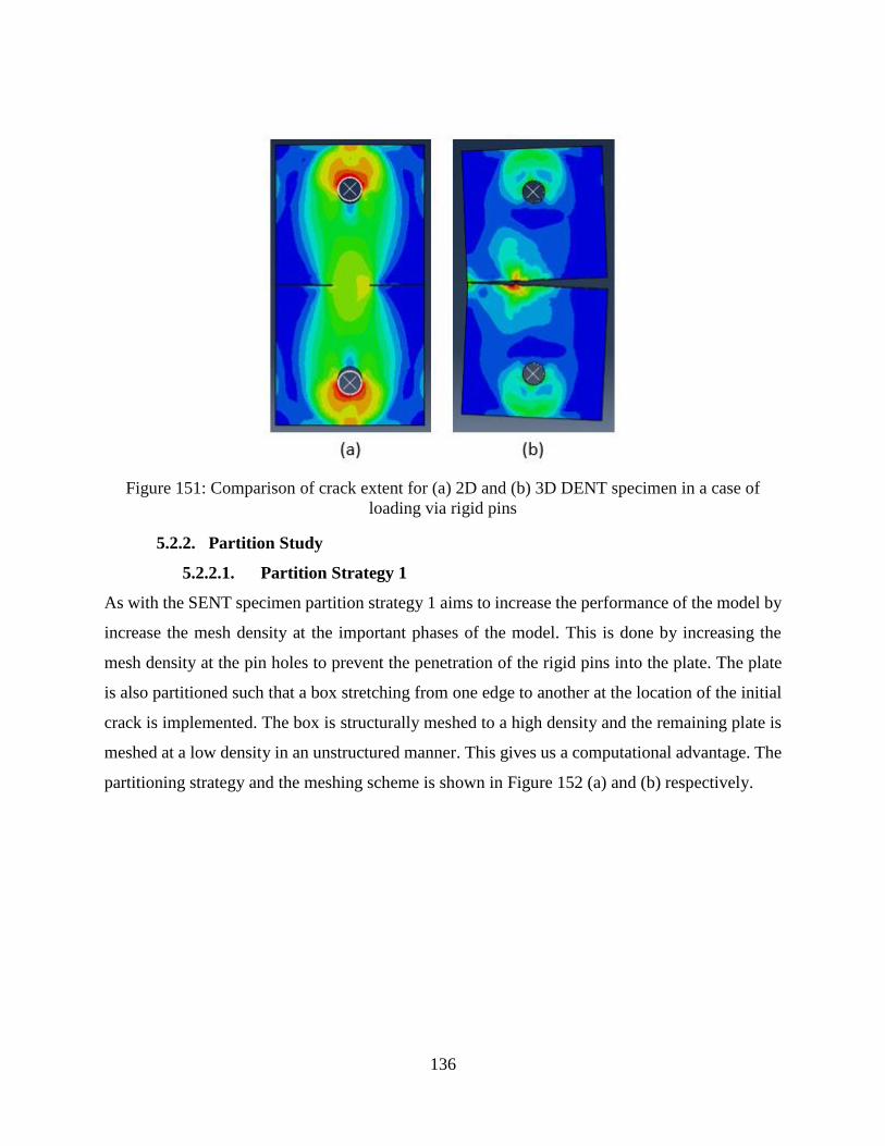
136
Figure 151: Comparison of crack extent for (a) 2D and (b) 3D DENT specimen in a case of
loading via rigid pins
5.2.2. Partition Study
5.2.2.1. Partition Strategy 1
As with the SENT specimen partition strategy 1 aims to increase the performance of the model by
increase the mesh density at the important phases of the model. This is done by increasing the
mesh density at the pin holes to prevent the penetration of the rigid pins into the plate. The plate
is also partitioned such that a box stretching from one edge to another at the location of the initial
crack is implemented. The box is structurally meshed to a high density and the remaining plate is
meshed at a low density in an unstructured manner. This gives us a computational advantage. The
partitioning strategy and the meshing scheme is shown in Figure 152 (a) and (b) respectively.
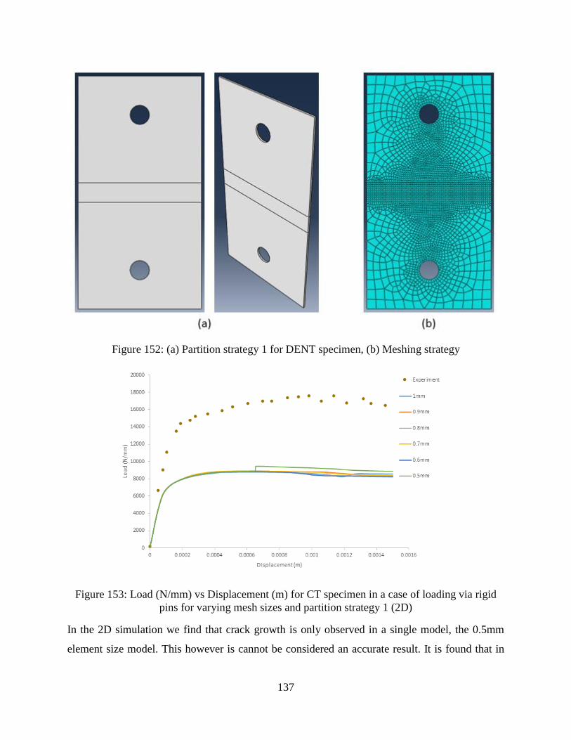
137
Figure 152: (a) Partition strategy 1 for DENT specimen, (b) Meshing strategy
Figure 153: Load (N/mm) vs Displacement (m) for CT specimen in a case of loading via rigid
pins for varying mesh sizes and partition strategy 1 (2D)
In the 2D simulation we find that crack growth is only observed in a single model, the 0.5mm
element size model. This however is cannot be considered an accurate result. It is found that in
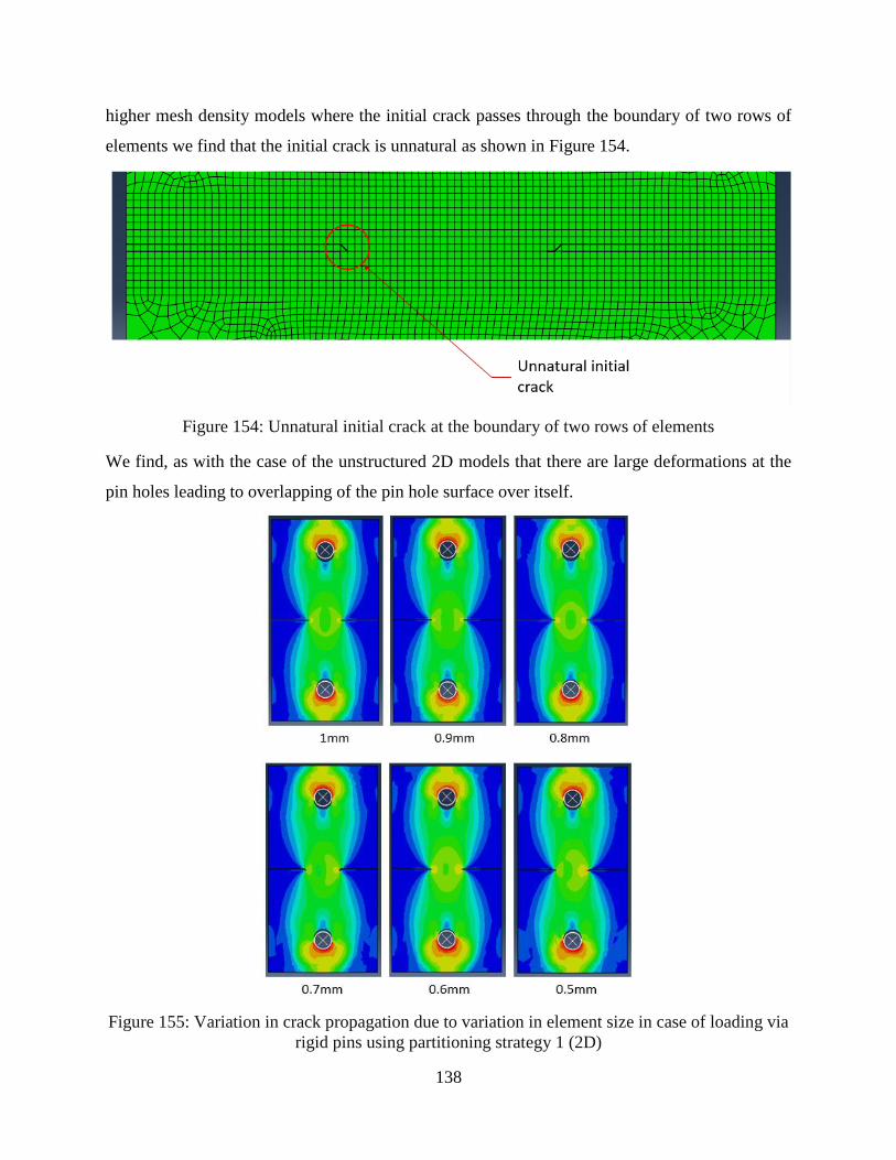
138
higher mesh density models where the initial crack passes through the boundary of two rows of
elements we find that the initial crack is unnatural as shown in Figure 154.
Figure 154: Unnatural initial crack at the boundary of two rows of elements
We find, as with the case of the unstructured 2D models that there are large deformations at the
pin holes leading to overlapping of the pin hole surface over itself.
Figure 155: Variation in crack propagation due to variation in element size in case of loading via
rigid pins using partitioning strategy 1 (2D)
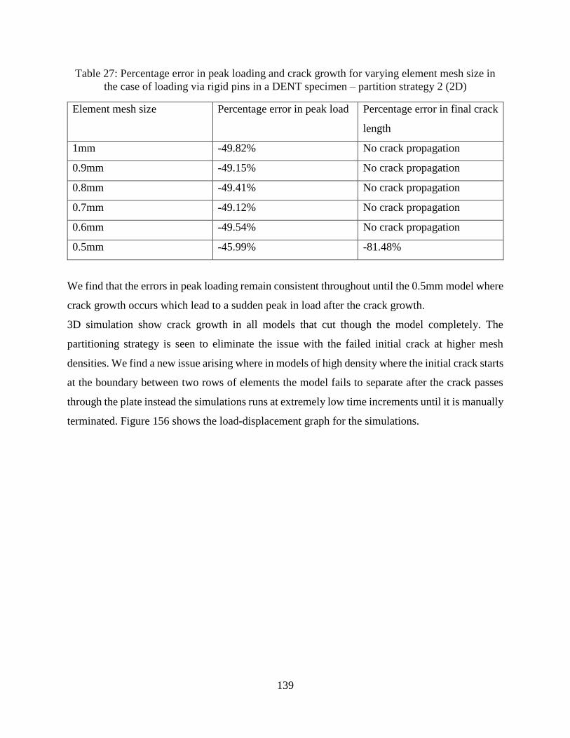
139
Table 27: Percentage error in peak loading and crack growth for varying element mesh size in
the case of loading via rigid pins in a DENT specimen – partition strategy 2 (2D)
Element mesh size Percentage error in peak load Percentage error in final crack
length
1mm -49.82% No crack propagation
0.9mm -49.15% No crack propagation
0.8mm -49.41% No crack propagation
0.7mm -49.12% No crack propagation
0.6mm -49.54% No crack propagation
0.5mm -45.99% -81.48%
We find that the errors in peak loading remain consistent throughout until the 0.5mm model where
crack growth occurs which lead to a sudden peak in load after the crack growth.
3D simulation show crack growth in all models that cut though the model completely. The
partitioning strategy is seen to eliminate the issue with the failed initial crack at higher mesh
densities. We find a new issue arising where in models of high density where the initial crack starts
at the boundary between two rows of elements the model fails to separate after the crack passes
through the plate instead the simulations runs at extremely low time increments until it is manually
terminated. Figure 156 shows the load-displacement graph for the simulations.
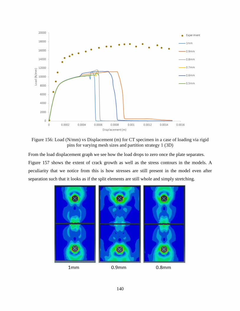
140
Figure 156: Load (N/mm) vs Displacement (m) for CT specimen in a case of loading via rigid
pins for varying mesh sizes and partition strategy 1 (3D)
From the load displacement graph we see how the load drops to zero once the plate separates.
Figure 157 shows the extent of crack growth as well as the stress contours in the models. A
peculiarity that we notice from this is how stresses are still present in the model even after
separation such that it looks as if the split elements are still whole and simply stretching.
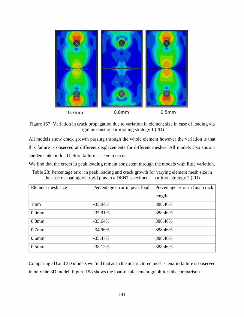
141
Figure 157: Variation in crack propagation due to variation in element size in case of loading via
rigid pins using partitioning strategy 1 (2D)
All models show crack growth passing through the whole element however the variation is that
this failure is observed at different displacements for different meshes. All models also show a
sudden spike in load before failure is seen to occur.
We find that the errors in peak loading remain consistent through the models with little variation.
Table 28: Percentage error in peak loading and crack growth for varying element mesh size in
the case of loading via rigid pins in a DENT specimen – partition strategy 2 (2D)
Element mesh size Percentage error in peak load Percentage error in final crack
length
1mm -35.94% 388.46%
0.9mm -35.91% 388.46%
0.8mm -33.64% 388.46%
0.7mm -34.96% 388.46%
0.6mm -35.47% 388.46%
0.5mm -38.12% 388.46%
Comparing 2D and 3D models we find that as in the unstructured mesh scenario failure is observed
in only the 3D model. Figure 158 shows the load-displacement graph for this comparison.
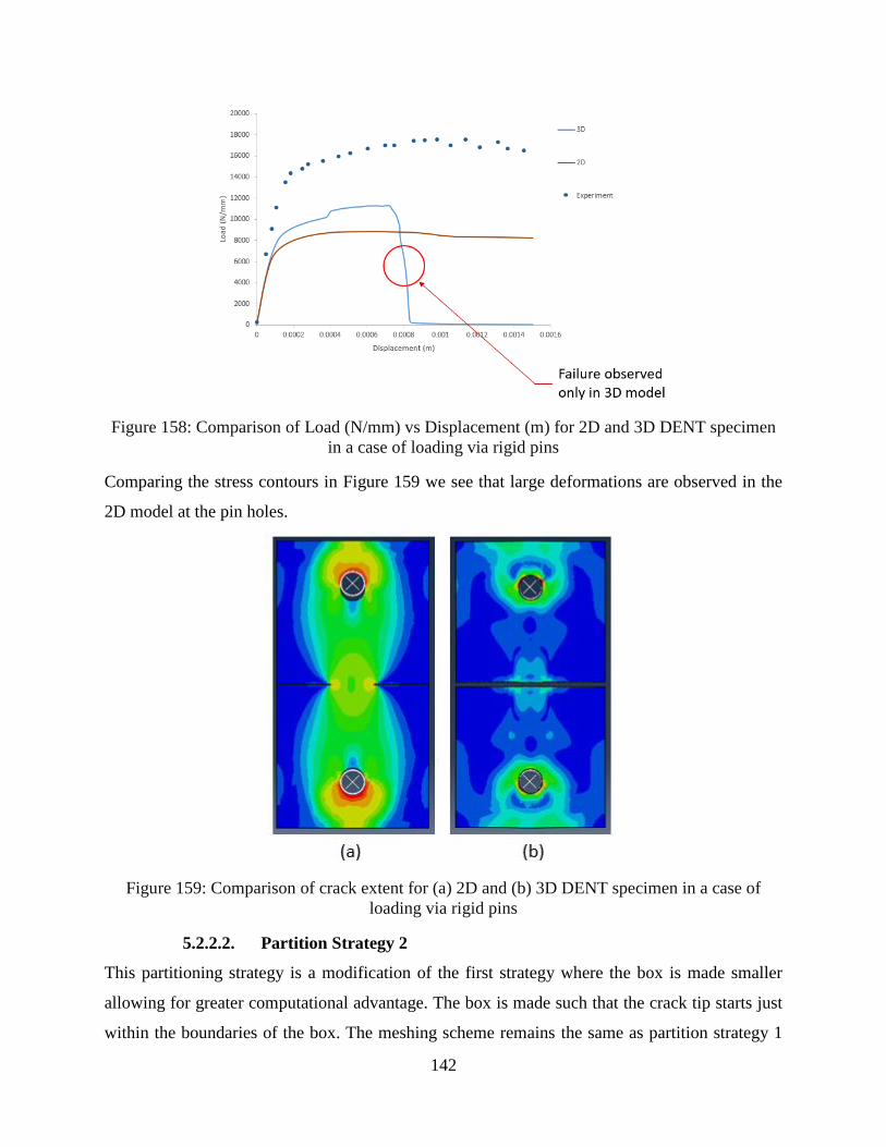
142
Figure 158: Comparison of Load (N/mm) vs Displacement (m) for 2D and 3D DENT specimen
in a case of loading via rigid pins
Comparing the stress contours in Figure 159 we see that large deformations are observed in the
2D model at the pin holes.
Figure 159: Comparison of crack extent for (a) 2D and (b) 3D DENT specimen in a case of
loading via rigid pins
5.2.2.2. Partition Strategy 2
This partitioning strategy is a modification of the first strategy where the box is made smaller
allowing for greater computational advantage. The box is made such that the crack tip starts just
within the boundaries of the box. The meshing scheme remains the same as partition strategy 1
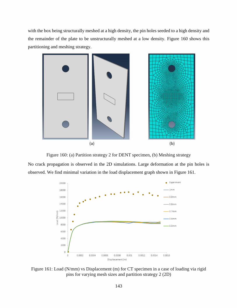
143
with the box being structurally meshed at a high density, the pin holes seeded to a high density and
the remainder of the plate to be unstructurally meshed at a low density. Figure 160 shows this
partitioning and meshing strategy.
Figure 160: (a) Partition strategy 2 for DENT specimen, (b) Meshing strategy
No crack propagation is observed in the 2D simulations. Large deformation at the pin holes is
observed. We find minimal variation in the load displacement graph shown in Figure 161.
Figure 161: Load (N/mm) vs Displacement (m) for CT specimen in a case of loading via rigid
pins for varying mesh sizes and partition strategy 2 (2D)
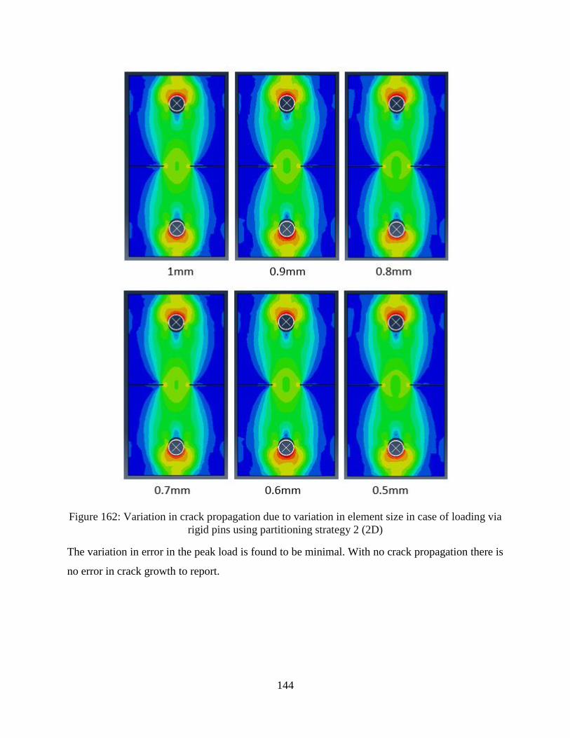
144
Figure 162: Variation in crack propagation due to variation in element size in case of loading via
rigid pins using partitioning strategy 2 (2D)
The variation in error in the peak load is found to be minimal. With no crack propagation there is
no error in crack growth to report.
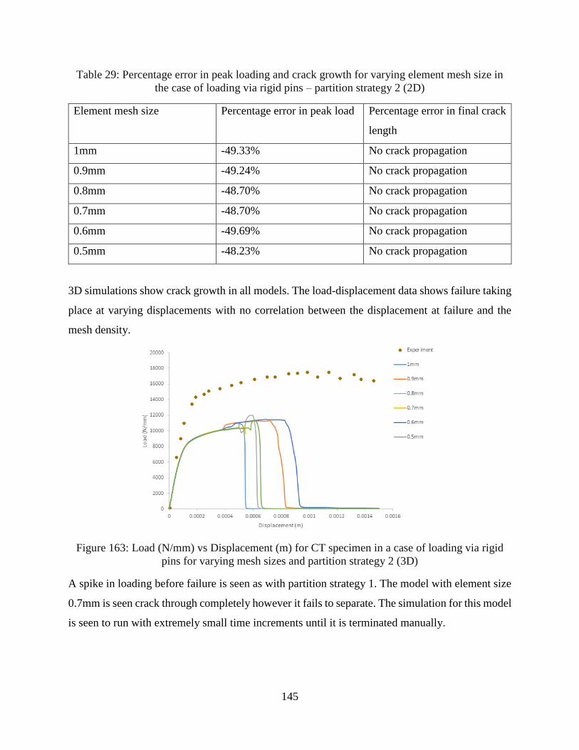
145
Table 29: Percentage error in peak loading and crack growth for varying element mesh size in
the case of loading via rigid pins – partition strategy 2 (2D)
Element mesh size Percentage error in peak load Percentage error in final crack
length
1mm -49.33% No crack propagation
0.9mm -49.24% No crack propagation
0.8mm -48.70% No crack propagation
0.7mm -48.70% No crack propagation
0.6mm -49.69% No crack propagation
0.5mm -48.23% No crack propagation
3D simulations show crack growth in all models. The load-displacement data shows failure taking
place at varying displacements with no correlation between the displacement at failure and the
mesh density.
Figure 163: Load (N/mm) vs Displacement (m) for CT specimen in a case of loading via rigid
pins for varying mesh sizes and partition strategy 2 (3D)
A spike in loading before failure is seen as with partition strategy 1. The model with element size
0.7mm is seen crack through completely however it fails to separate. The simulation for this model
is seen to run with extremely small time increments until it is terminated manually.
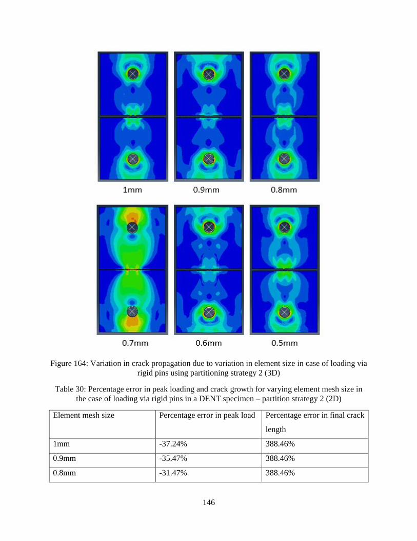
146
Figure 164: Variation in crack propagation due to variation in element size in case of loading via
rigid pins using partitioning strategy 2 (3D)
Table 30: Percentage error in peak loading and crack growth for varying element mesh size in
the case of loading via rigid pins in a DENT specimen – partition strategy 2 (2D)
Element mesh size Percentage error in peak load Percentage error in final crack
length
1mm -37.24% 388.46%
0.9mm -35.47% 388.46%
0.8mm -31.47% 388.46%
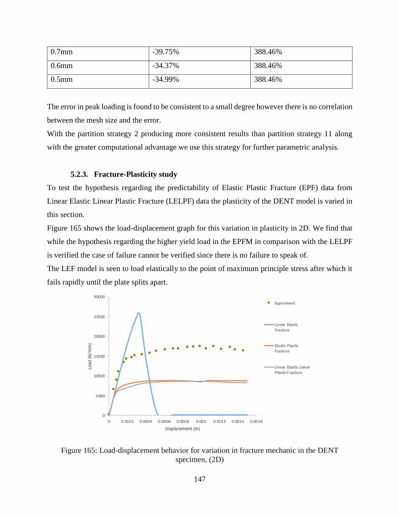
147
0.7mm -39.75% 388.46%
0.6mm -34.37% 388.46%
0.5mm -34.99% 388.46%
The error in peak loading is found to be consistent to a small degree however there is no correlation
between the mesh size and the error.
With the partition strategy 2 producing more consistent results than partition strategy 11 along
with the greater computational advantage we use this strategy for further parametric analysis.
5.2.3. Fracture-Plasticity study
To test the hypothesis regarding the predictability of Elastic Plastic Fracture (EPF) data from
Linear Elastic Linear Plastic Fracture (LELPF) data the plasticity of the DENT model is varied in
this section.
Figure 165 shows the load-displacement graph for this variation in plasticity in 2D. We find that
while the hypothesis regarding the higher yield load in the EPFM in comparison with the LELPF
is verified the case of failure cannot be verified since there is no failure to speak of.
The LEF model is seen to load elastically to the point of maximum principle stress after which it
fails rapidly until the plate splits apart.
Figure 165: Load-displacement behavior for variation in fracture mechanic in the DENT
specimen, (2D)
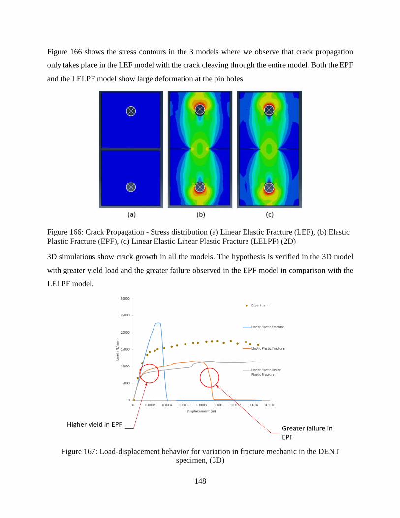
148
Figure 166 shows the stress contours in the 3 models where we observe that crack propagation
only takes place in the LEF model with the crack cleaving through the entire model. Both the EPF
and the LELPF model show large deformation at the pin holes
Figure 166: Crack Propagation - Stress distribution (a) Linear Elastic Fracture (LEF), (b) Elastic
Plastic Fracture (EPF), (c) Linear Elastic Linear Plastic Fracture (LELPF) (2D)
3D simulations show crack growth in all the models. The hypothesis is verified in the 3D model
with greater yield load and the greater failure observed in the EPF model in comparison with the
LELPF model.
Figure 167: Load-displacement behavior for variation in fracture mechanic in the DENT
specimen, (3D)
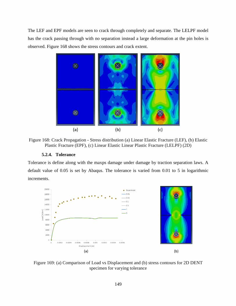
149
The LEF and EPF models are seen to crack through completely and separate. The LELPF model
has the crack passing through with no separation instead a large deformation at the pin holes is
observed. Figure 168 shows the stress contours and crack extent.
Figure 168: Crack Propagation - Stress distribution (a) Linear Elastic Fracture (LEF), (b) Elastic
Plastic Fracture (EPF), (c) Linear Elastic Linear Plastic Fracture (LELPF) (2D)
5.2.4. Tolerance
Tolerance is define along with the maxps damage under damage by traction separation laws. A
default value of 0.05 is set by Abaqus. The tolerance is varied from 0.01 to 5 in logarithmic
increments.
Figure 169: (a) Comparison of Load vs Displacement and (b) stress contours for 2D DENT
specimen for varying tolerance
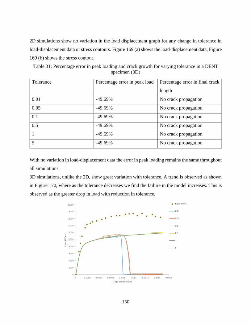
150
2D simulations show no variation in the load displacement graph for any change in tolerance in
load-displacement data or stress contours. Figure 169 (a) shows the load-displacement data, Figure
169 (b) shows the stress contour.
Table 31: Percentage error in peak loading and crack growth for varying tolerance in a DENT
specimen (3D)
Tolerance Percentage error in peak load Percentage error in final crack
length
0.01 -49.69% No crack propagation
0.05 -49.69% No crack propagation
0.1 -49.69% No crack propagation
0.5 -49.69% No crack propagation
1 -49.69% No crack propagation
5 -49.69% No crack propagation
With no variation in load-displacement data the error in peak loading remains the same throughout
all simulations.
3D simulations, unlike the 2D, show great variation with tolerance. A trend is observed as shown
in Figure 170, where as the tolerance decreases we find the failure in the model increases. This is
observed as the greater drop in load with reduction in tolerance.
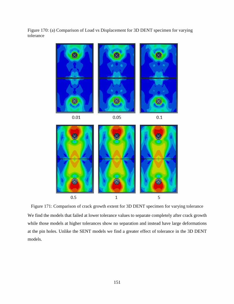
151
Figure 170: (a) Comparison of Load vs Displacement for 3D DENT specimen for varying
tolerance
Figure 171: Comparison of crack growth extent for 3D DENT specimen for varying tolerance
We find the models that failed at lower tolerance values to separate completely after crack growth
while those models at higher tolerances show no separation and instead have large deformations
at the pin holes. Unlike the SENT models we find a greater effect of tolerance in the 3D DENT
models.

152
Table 32: Percentage error in peak loading and crack growth for varying tolerance in a DENT
specimen (3D)
Tolerance Percentage error in peak load Percentage error in final crack
length
0.01 -33.48% 388.46%
0.05 -34.37% 388.46%
0.1 -35.94% 388.46%
0.5 -30.53% 388.46%
1 -31.91% 388.46%
5 -31.91% 388.46%
No large variation in peak loads is observed with change in tolerance in the 3D model.
5.2.5. Damage Stability Cohesive
In 2D simulations we find no variation in load-displacement data or stress contours with any
change in damage stability cohesive. No crack growth is observed in any model. Figure 172 (a)
shows the load-displacement data, Figure 172 (b) shows the stress contour.
Figure 172: (a) Comparison of Load vs Displacement and (b) stress contours for 2D DENT
specimen for varying Damage Stability Cohesive
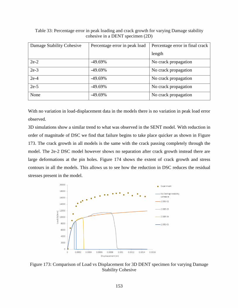
153
Table 33: Percentage error in peak loading and crack growth for varying Damage stability
cohesive in a DENT specimen (2D)
Damage Stability Cohesive Percentage error in peak load Percentage error in final crack
length
2e-2 -49.69% No crack propagation
2e-3 -49.69% No crack propagation
2e-4 -49.69% No crack propagation
2e-5 -49.69% No crack propagation
None -49.69% No crack propagation
With no variation in load-displacement data in the models there is no variation in peak load error
observed.
3D simulations show a similar trend to what was observed in the SENT model. With reduction in
order of magnitude of DSC we find that failure begins to take place quicker as shown in Figure
173. The crack growth in all models is the same with the crack passing completely through the
model. The 2e-2 DSC model however shows no separation after crack growth instead there are
large deformations at the pin holes. Figure 174 shows the extent of crack growth and stress
contours in all the models. This allows us to see how the reduction in DSC reduces the residual
stresses present in the model.
Figure 173: Comparison of Load vs Displacement for 3D DENT specimen for varying Damage
Stability Cohesive
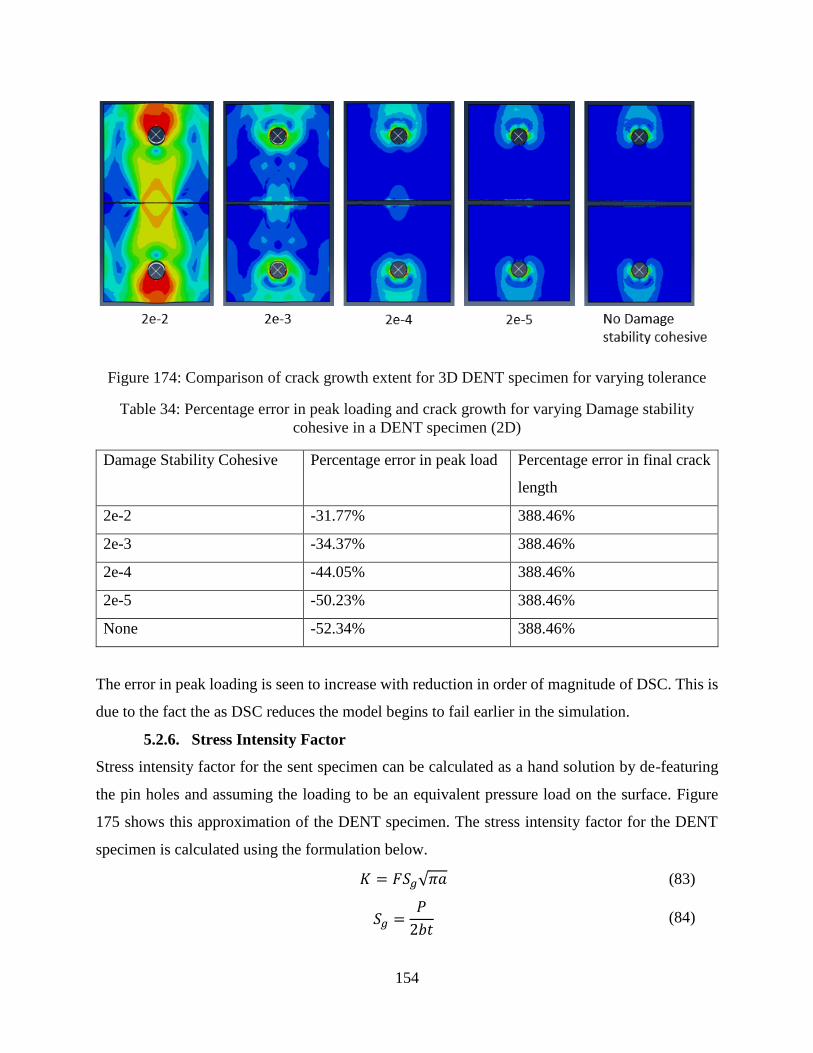
154
Figure 174: Comparison of crack growth extent for 3D DENT specimen for varying tolerance
Table 34: Percentage error in peak loading and crack growth for varying Damage stability
cohesive in a DENT specimen (2D)
Damage Stability Cohesive Percentage error in peak load Percentage error in final crack
length
2e-2 -31.77% 388.46%
2e-3 -34.37% 388.46%
2e-4 -44.05% 388.46%
2e-5 -50.23% 388.46%
None -52.34% 388.46%
The error in peak loading is seen to increase with reduction in order of magnitude of DSC. This is
due to the fact the as DSC reduces the model begins to fail earlier in the simulation.
5.2.6. Stress Intensity Factor
Stress intensity factor for the sent specimen can be calculated as a hand solution by de-featuring
the pin holes and assuming the loading to be an equivalent pressure load on the surface. Figure
175 shows this approximation of the DENT specimen. The stress intensity factor for the DENT
specimen is calculated using the formulation below.
𝐾 = 𝐹𝑆𝑔√𝜋𝑎 (83)
𝑆𝑔 =𝑃
2𝑏𝑡 (84)
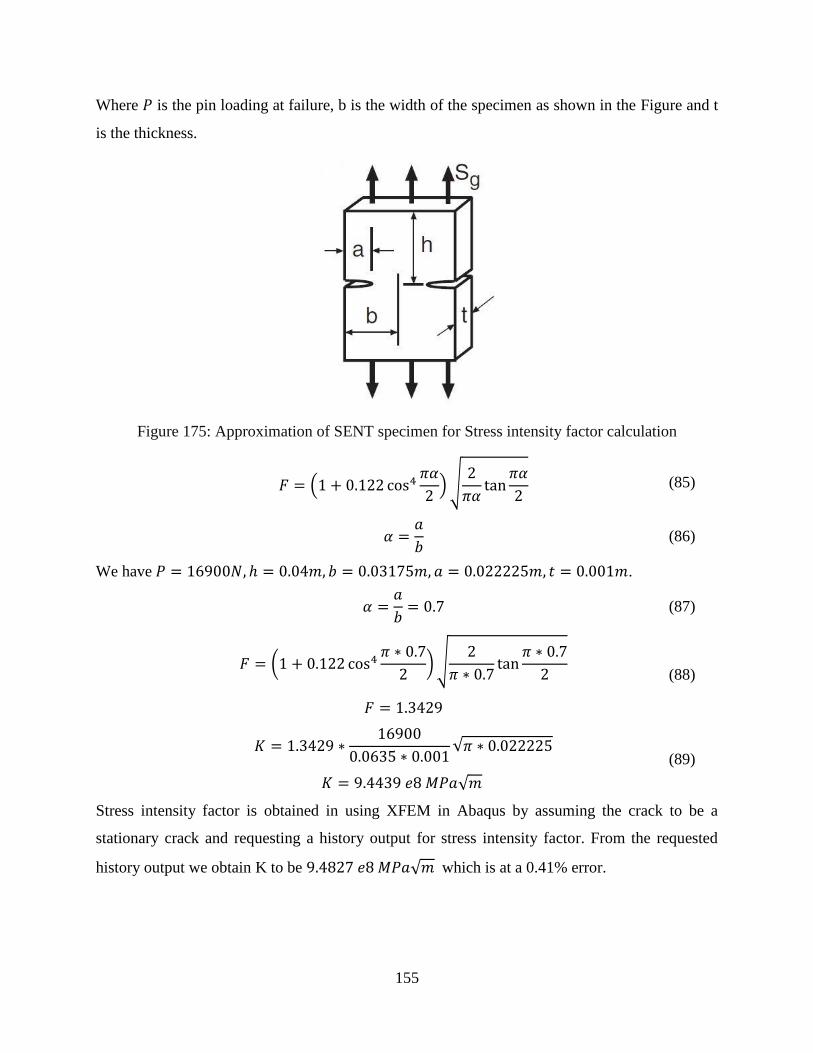
155
Where 𝑃 is the pin loading at failure, b is the width of the specimen as shown in the Figure and t
is the thickness.
Figure 175: Approximation of SENT specimen for Stress intensity factor calculation
𝐹 = (1 + 0.122 cos4𝜋𝛼
2)√
2
𝜋𝛼tan
𝜋𝛼
2 (85)
𝛼 =𝑎
𝑏 (86)
We have 𝑃 = 16900𝑁, ℎ = 0.04𝑚, 𝑏 = 0.03175𝑚, 𝑎 = 0.022225𝑚, 𝑡 = 0.001𝑚.
𝛼 =𝑎
𝑏= 0.7 (87)
𝐹 = (1 + 0.122 cos4
𝜋 ∗ 0.7
2)√
2
𝜋 ∗ 0.7tan
𝜋 ∗ 0.7
2
𝐹 = 1.3429
(88)
𝐾 = 1.3429 ∗
16900
0.0635 ∗ 0.001√𝜋 ∗ 0.022225
𝐾 = 9.4439 𝑒8 𝑀𝑃𝑎√𝑚
(89)
Stress intensity factor is obtained in using XFEM in Abaqus by assuming the crack to be a
stationary crack and requesting a history output for stress intensity factor. From the requested
history output we obtain K to be 9.4827 𝑒8 𝑀𝑃𝑎√𝑚 which is at a 0.41% error.
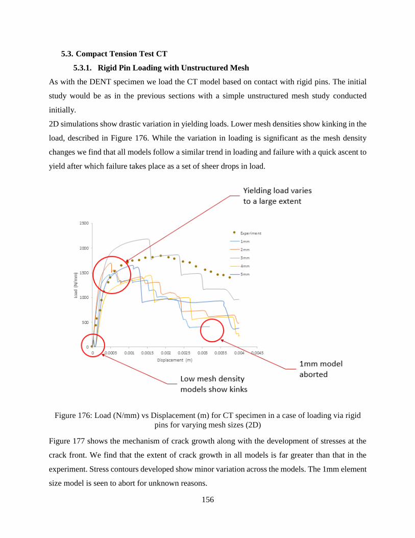
156
5.3. Compact Tension Test CT
5.3.1. Rigid Pin Loading with Unstructured Mesh
As with the DENT specimen we load the CT model based on contact with rigid pins. The initial
study would be as in the previous sections with a simple unstructured mesh study conducted
initially.
2D simulations show drastic variation in yielding loads. Lower mesh densities show kinking in the
load, described in Figure 176. While the variation in loading is significant as the mesh density
changes we find that all models follow a similar trend in loading and failure with a quick ascent to
yield after which failure takes place as a set of sheer drops in load.
Figure 176: Load (N/mm) vs Displacement (m) for CT specimen in a case of loading via rigid
pins for varying mesh sizes (2D)
Figure 177 shows the mechanism of crack growth along with the development of stresses at the
crack front. We find that the extent of crack growth in all models is far greater than that in the
experiment. Stress contours developed show minor variation across the models. The 1mm element
size model is seen to abort for unknown reasons.
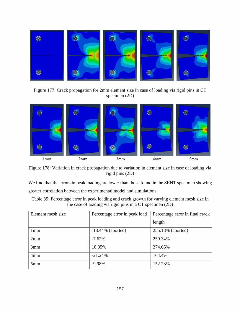
157
Figure 177: Crack propagation for 2mm element size in case of loading via rigid pins in CT
specimen (2D)
Figure 178: Variation in crack propagation due to variation in element size in case of loading via
rigid pins (2D)
We find that the errors in peak loading are lower than those found in the SENT specimen showing
greater correlation between the experimental model and simulations.
Table 35: Percentage error in peak loading and crack growth for varying element mesh size in
the case of loading via rigid pins in a CT specimen (2D)
Element mesh size Percentage error in peak load Percentage error in final crack
length
1mm -18.44% (aborted) 255.18% (aborted)
2mm -7.62% 259.34%
3mm 18.85% 274.66%
4mm -21.24% 164.4%
5mm -9.98% 152.23%
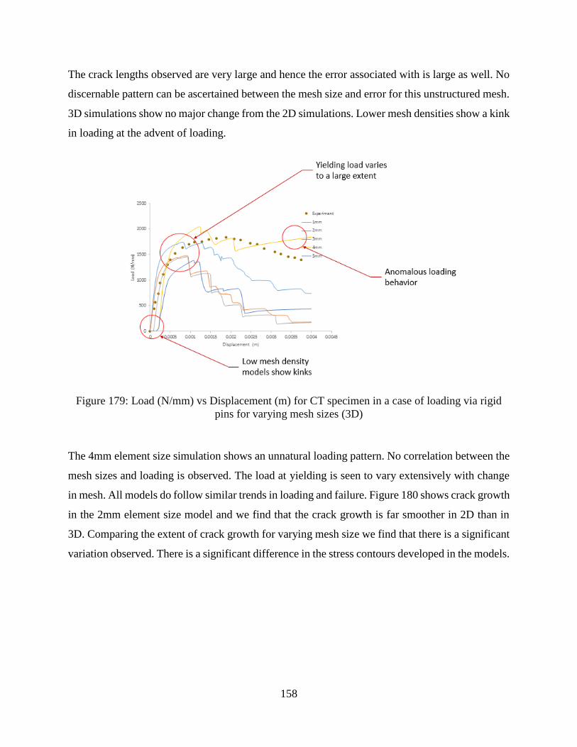
158
The crack lengths observed are very large and hence the error associated with is large as well. No
discernable pattern can be ascertained between the mesh size and error for this unstructured mesh.
3D simulations show no major change from the 2D simulations. Lower mesh densities show a kink
in loading at the advent of loading.
Figure 179: Load (N/mm) vs Displacement (m) for CT specimen in a case of loading via rigid
pins for varying mesh sizes (3D)
The 4mm element size simulation shows an unnatural loading pattern. No correlation between the
mesh sizes and loading is observed. The load at yielding is seen to vary extensively with change
in mesh. All models do follow similar trends in loading and failure. Figure 180 shows crack growth
in the 2mm element size model and we find that the crack growth is far smoother in 2D than in
3D. Comparing the extent of crack growth for varying mesh size we find that there is a significant
variation observed. There is a significant difference in the stress contours developed in the models.
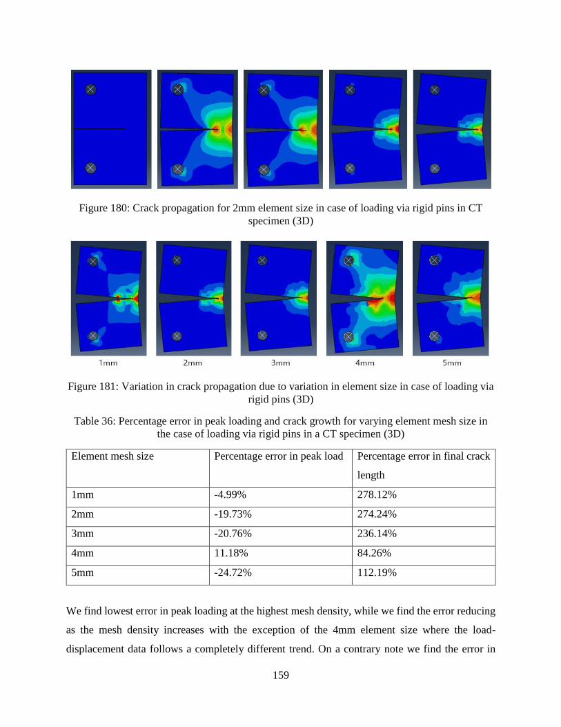
159
Figure 180: Crack propagation for 2mm element size in case of loading via rigid pins in CT
specimen (3D)
Figure 181: Variation in crack propagation due to variation in element size in case of loading via
rigid pins (3D)
Table 36: Percentage error in peak loading and crack growth for varying element mesh size in
the case of loading via rigid pins in a CT specimen (3D)
Element mesh size Percentage error in peak load Percentage error in final crack
length
1mm -4.99% 278.12%
2mm -19.73% 274.24%
3mm -20.76% 236.14%
4mm 11.18% 84.26%
5mm -24.72% 112.19%
We find lowest error in peak loading at the highest mesh density, while we find the error reducing
as the mesh density increases with the exception of the 4mm element size where the load-
displacement data follows a completely different trend. On a contrary note we find the error in
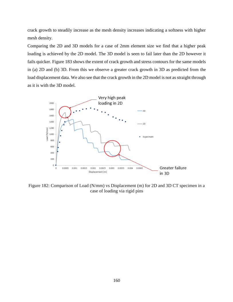
160
crack growth to steadily increase as the mesh density increases indicating a softness with higher
mesh density.
Comparing the 2D and 3D models for a case of 2mm element size we find that a higher peak
loading is achieved by the 2D model. The 3D model is seen to fail later than the 2D however it
fails quicker. Figure 183 shows the extent of crack growth and stress contours for the same models
in (a) 2D and (b) 3D. From this we observe a greater crack growth in 3D as predicted from the
load displacement data. We also see that the crack growth in the 2D model is not as straight through
as it is with the 3D model.
Figure 182: Comparison of Load (N/mm) vs Displacement (m) for 2D and 3D CT specimen in a
case of loading via rigid pins
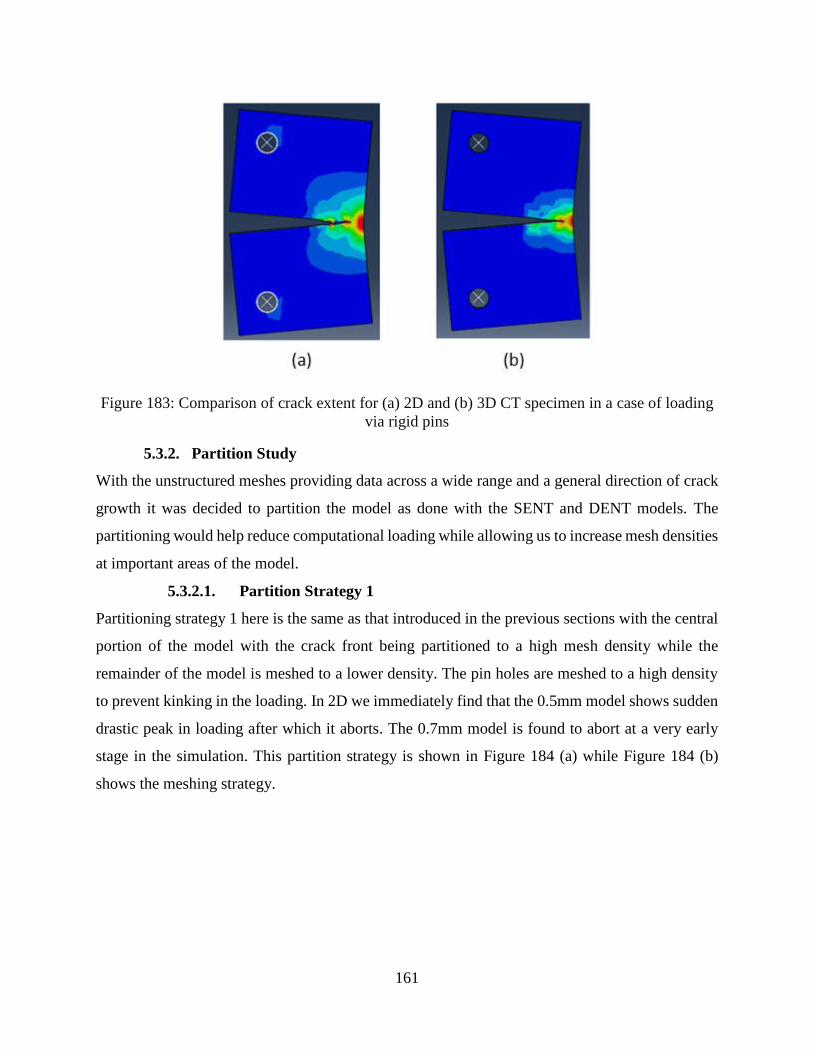
161
Figure 183: Comparison of crack extent for (a) 2D and (b) 3D CT specimen in a case of loading
via rigid pins
5.3.2. Partition Study
With the unstructured meshes providing data across a wide range and a general direction of crack
growth it was decided to partition the model as done with the SENT and DENT models. The
partitioning would help reduce computational loading while allowing us to increase mesh densities
at important areas of the model.
5.3.2.1. Partition Strategy 1
Partitioning strategy 1 here is the same as that introduced in the previous sections with the central
portion of the model with the crack front being partitioned to a high mesh density while the
remainder of the model is meshed to a lower density. The pin holes are meshed to a high density
to prevent kinking in the loading. In 2D we immediately find that the 0.5mm model shows sudden
drastic peak in loading after which it aborts. The 0.7mm model is found to abort at a very early
stage in the simulation. This partition strategy is shown in Figure 184 (a) while Figure 184 (b)
shows the meshing strategy.
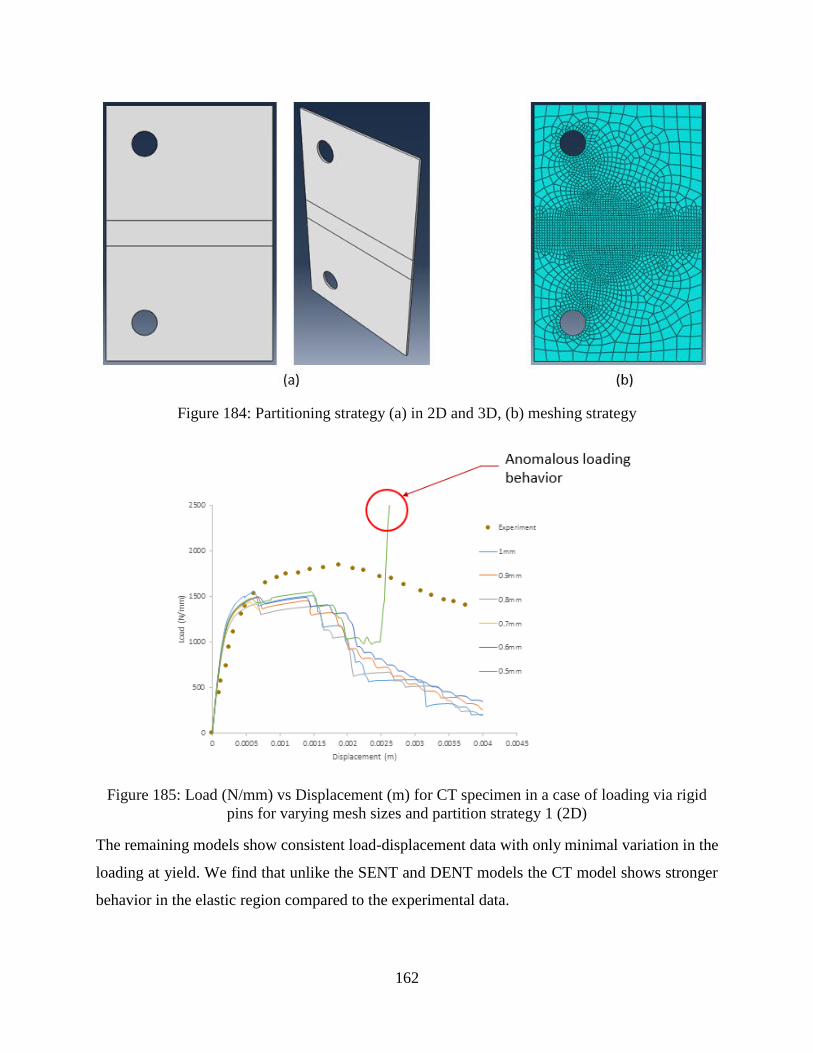
162
Figure 184: Partitioning strategy (a) in 2D and 3D, (b) meshing strategy
Figure 185: Load (N/mm) vs Displacement (m) for CT specimen in a case of loading via rigid
pins for varying mesh sizes and partition strategy 1 (2D)
The remaining models show consistent load-displacement data with only minimal variation in the
loading at yield. We find that unlike the SENT and DENT models the CT model shows stronger
behavior in the elastic region compared to the experimental data.
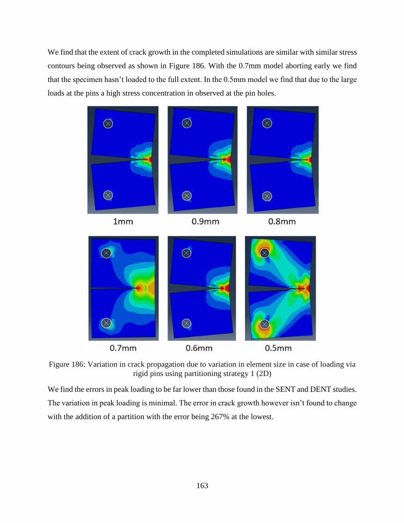
163
We find that the extent of crack growth in the completed simulations are similar with similar stress
contours being observed as shown in Figure 186. With the 0.7mm model aborting early we find
that the specimen hasn’t loaded to the full extent. In the 0.5mm model we find that due to the large
loads at the pins a high stress concentration in observed at the pin holes.
Figure 186: Variation in crack propagation due to variation in element size in case of loading via
rigid pins using partitioning strategy 1 (2D)
We find the errors in peak loading to be far lower than those found in the SENT and DENT studies.
The variation in peak loading is minimal. The error in crack growth however isn’t found to change
with the addition of a partition with the error being 267% at the lowest.
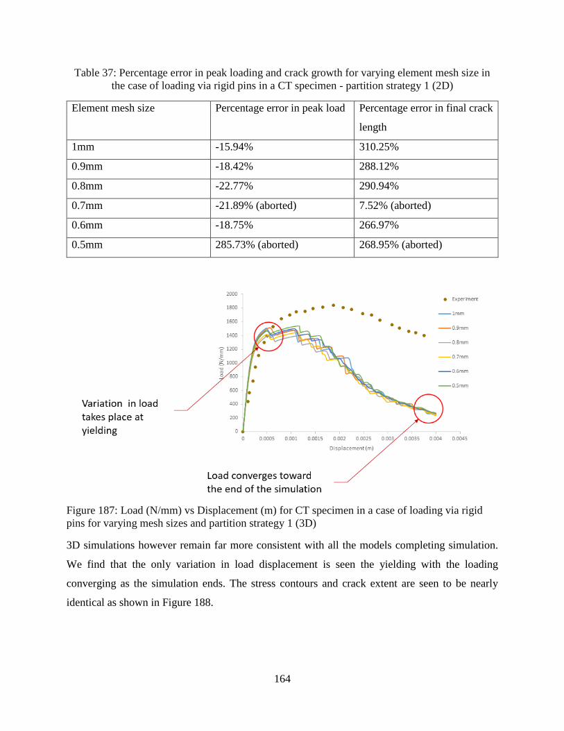
164
Table 37: Percentage error in peak loading and crack growth for varying element mesh size in
the case of loading via rigid pins in a CT specimen - partition strategy 1 (2D)
Element mesh size Percentage error in peak load Percentage error in final crack
length
1mm -15.94% 310.25%
0.9mm -18.42% 288.12%
0.8mm -22.77% 290.94%
0.7mm -21.89% (aborted) 7.52% (aborted)
0.6mm -18.75% 266.97%
0.5mm 285.73% (aborted) 268.95% (aborted)
Figure 187: Load (N/mm) vs Displacement (m) for CT specimen in a case of loading via rigid
pins for varying mesh sizes and partition strategy 1 (3D)
3D simulations however remain far more consistent with all the models completing simulation.
We find that the only variation in load displacement is seen the yielding with the loading
converging as the simulation ends. The stress contours and crack extent are seen to be nearly
identical as shown in Figure 188.
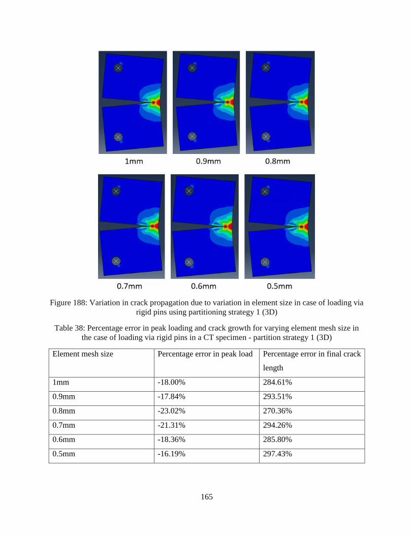
165
Figure 188: Variation in crack propagation due to variation in element size in case of loading via
rigid pins using partitioning strategy 1 (3D)
Table 38: Percentage error in peak loading and crack growth for varying element mesh size in
the case of loading via rigid pins in a CT specimen - partition strategy 1 (3D)
Element mesh size Percentage error in peak load Percentage error in final crack
length
1mm -18.00% 284.61%
0.9mm -17.84% 293.51%
0.8mm -23.02% 270.36%
0.7mm -21.31% 294.26%
0.6mm -18.36% 285.80%
0.5mm -16.19% 297.43%
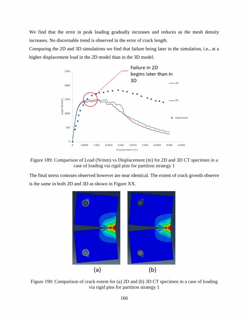
166
We find that the error in peak loading gradually increases and reduces as the mesh density
increases. No discernable trend is observed in the error of crack length.
Comparing the 2D and 3D simulations we find that failure being later in the simulation, i.e., at a
higher displacement load in the 2D model than in the 3D model.
Figure 189: Comparison of Load (N/mm) vs Displacement (m) for 2D and 3D CT specimen in a
case of loading via rigid pins for partition strategy 1
The final stress contours observed however are near identical. The extent of crack growth observe
is the same in both 2D and 3D as shown in Figure XX.
Figure 190: Comparison of crack extent for (a) 2D and (b) 3D CT specimen in a case of loading
via rigid pins for partition strategy 1
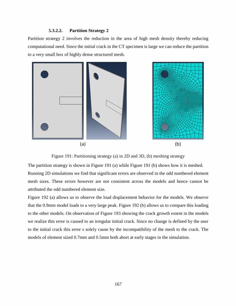
167
5.3.2.2. Partition Strategy 2
Partition strategy 2 involves the reduction in the area of high mesh density thereby reducing
computational need. Since the initial crack in the CT specimen is large we can reduce the partition
to a very small box of highly dense structured mesh.
Figure 191: Partitioning strategy (a) in 2D and 3D, (b) meshing strategy
The partition strategy is shown in Figure 191 (a) while Figure 191 (b) shows how it is meshed.
Running 2D simulations we find that significant errors are observed in the odd numbered element
mesh sizes. These errors however are not consistent across the models and hence cannot be
attributed the odd numbered element size.
Figure 192 (a) allows us to observe the load displacement behavior for the models. We observe
that the 0.9mm model loads to a very large peak. Figure 192 (b) allows us to compare this loading
to the other models. On observation of Figure 193 showing the crack growth extent in the models
we realize this error is caused to an irregular initial crack. Since no change is defined by the user
to the initial crack this error s solely cause by the incompatibility of the mesh to the crack. The
models of element sized 0.7mm and 0.5mm both abort at early stages in the simulation.
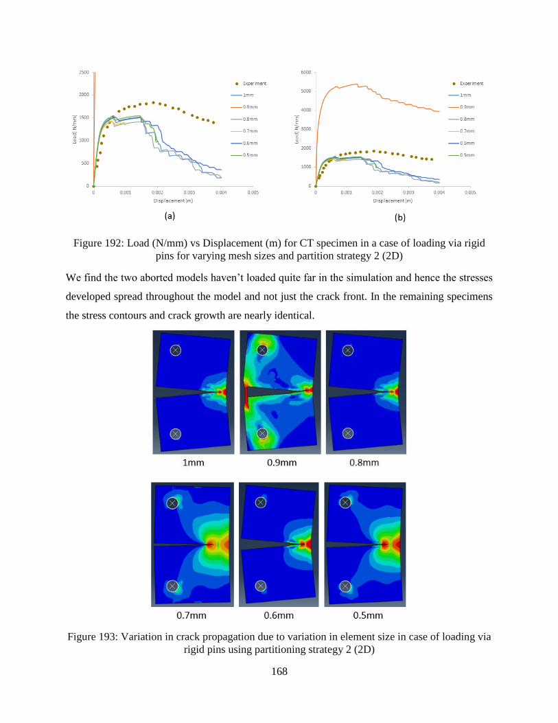
168
Figure 192: Load (N/mm) vs Displacement (m) for CT specimen in a case of loading via rigid
pins for varying mesh sizes and partition strategy 2 (2D)
We find the two aborted models haven’t loaded quite far in the simulation and hence the stresses
developed spread throughout the model and not just the crack front. In the remaining specimens
the stress contours and crack growth are nearly identical.
Figure 193: Variation in crack propagation due to variation in element size in case of loading via
rigid pins using partitioning strategy 2 (2D)
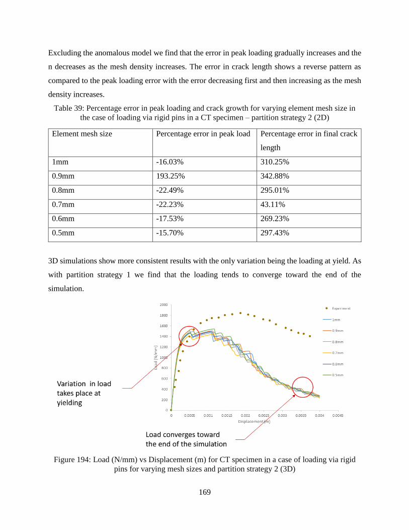
169
Excluding the anomalous model we find that the error in peak loading gradually increases and the
n decreases as the mesh density increases. The error in crack length shows a reverse pattern as
compared to the peak loading error with the error decreasing first and then increasing as the mesh
density increases.
Table 39: Percentage error in peak loading and crack growth for varying element mesh size in
the case of loading via rigid pins in a CT specimen – partition strategy 2 (2D)
Element mesh size Percentage error in peak load Percentage error in final crack
length
1mm -16.03% 310.25%
0.9mm 193.25% 342.88%
0.8mm -22.49% 295.01%
0.7mm -22.23% 43.11%
0.6mm -17.53% 269.23%
0.5mm -15.70% 297.43%
3D simulations show more consistent results with the only variation being the loading at yield. As
with partition strategy 1 we find that the loading tends to converge toward the end of the
simulation.
Figure 194: Load (N/mm) vs Displacement (m) for CT specimen in a case of loading via rigid
pins for varying mesh sizes and partition strategy 2 (3D)
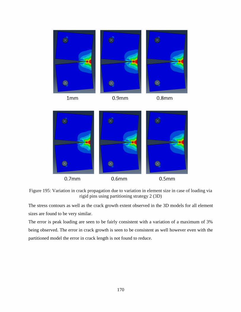
170
Figure 195: Variation in crack propagation due to variation in element size in case of loading via
rigid pins using partitioning strategy 2 (3D)
The stress contours as well as the crack growth extent observed in the 3D models for all element
sizes are found to be very similar.
The error is peak loading are seen to be fairly consistent with a variation of a maximum of 3%
being observed. The error in crack growth is seen to be consistent as well however even with the
partitioned model the error in crack length is not found to reduce.
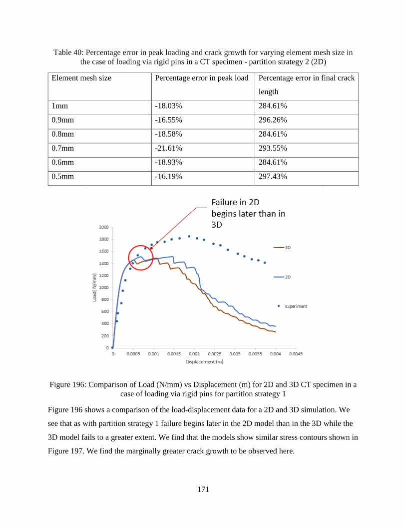
171
Table 40: Percentage error in peak loading and crack growth for varying element mesh size in
the case of loading via rigid pins in a CT specimen - partition strategy 2 (2D)
Element mesh size Percentage error in peak load Percentage error in final crack
length
1mm -18.03% 284.61%
0.9mm -16.55% 296.26%
0.8mm -18.58% 284.61%
0.7mm -21.61% 293.55%
0.6mm -18.93% 284.61%
0.5mm -16.19% 297.43%
Figure 196: Comparison of Load (N/mm) vs Displacement (m) for 2D and 3D CT specimen in a
case of loading via rigid pins for partition strategy 1
Figure 196 shows a comparison of the load-displacement data for a 2D and 3D simulation. We
see that as with partition strategy 1 failure begins later in the 2D model than in the 3D while the
3D model fails to a greater extent. We find that the models show similar stress contours shown in
Figure 197. We find the marginally greater crack growth to be observed here.
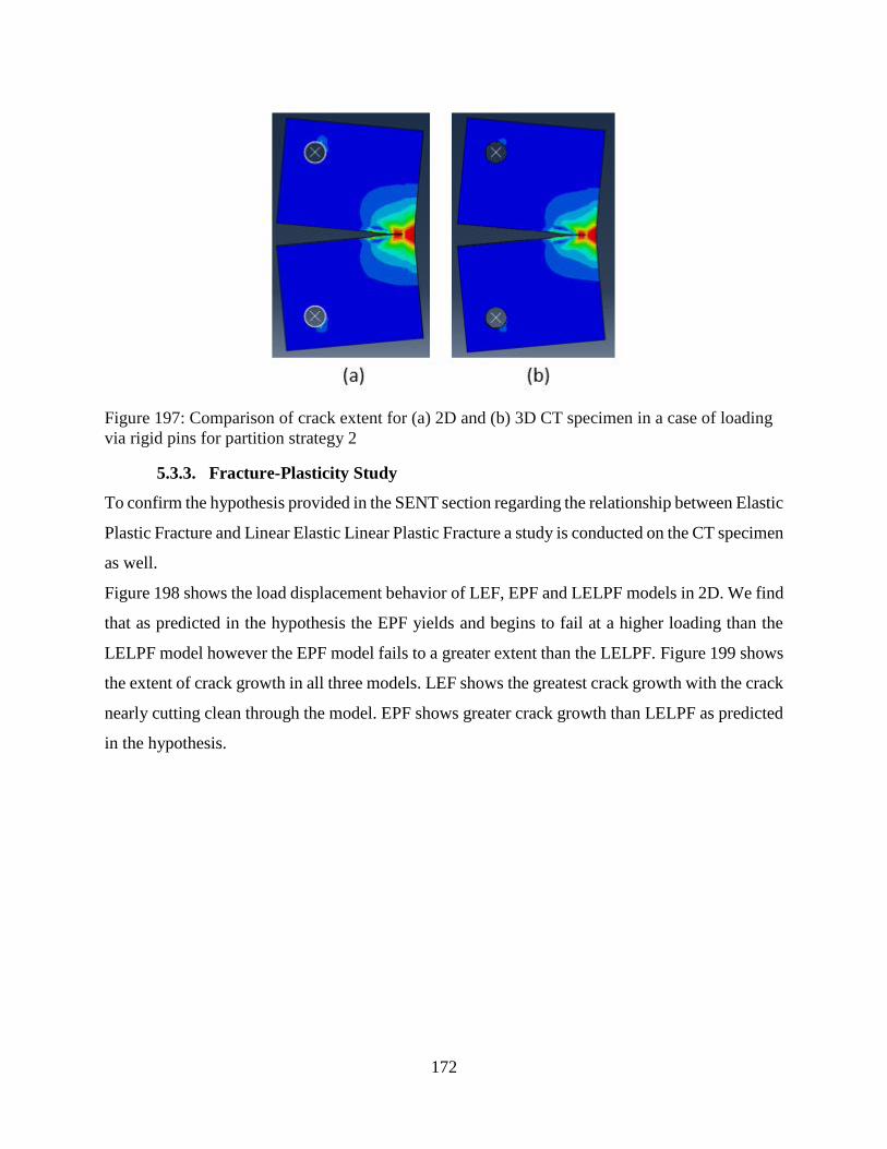
172
Figure 197: Comparison of crack extent for (a) 2D and (b) 3D CT specimen in a case of loading
via rigid pins for partition strategy 2
5.3.3. Fracture-Plasticity Study
To confirm the hypothesis provided in the SENT section regarding the relationship between Elastic
Plastic Fracture and Linear Elastic Linear Plastic Fracture a study is conducted on the CT specimen
as well.
Figure 198 shows the load displacement behavior of LEF, EPF and LELPF models in 2D. We find
that as predicted in the hypothesis the EPF yields and begins to fail at a higher loading than the
LELPF model however the EPF model fails to a greater extent than the LELPF. Figure 199 shows
the extent of crack growth in all three models. LEF shows the greatest crack growth with the crack
nearly cutting clean through the model. EPF shows greater crack growth than LELPF as predicted
in the hypothesis.
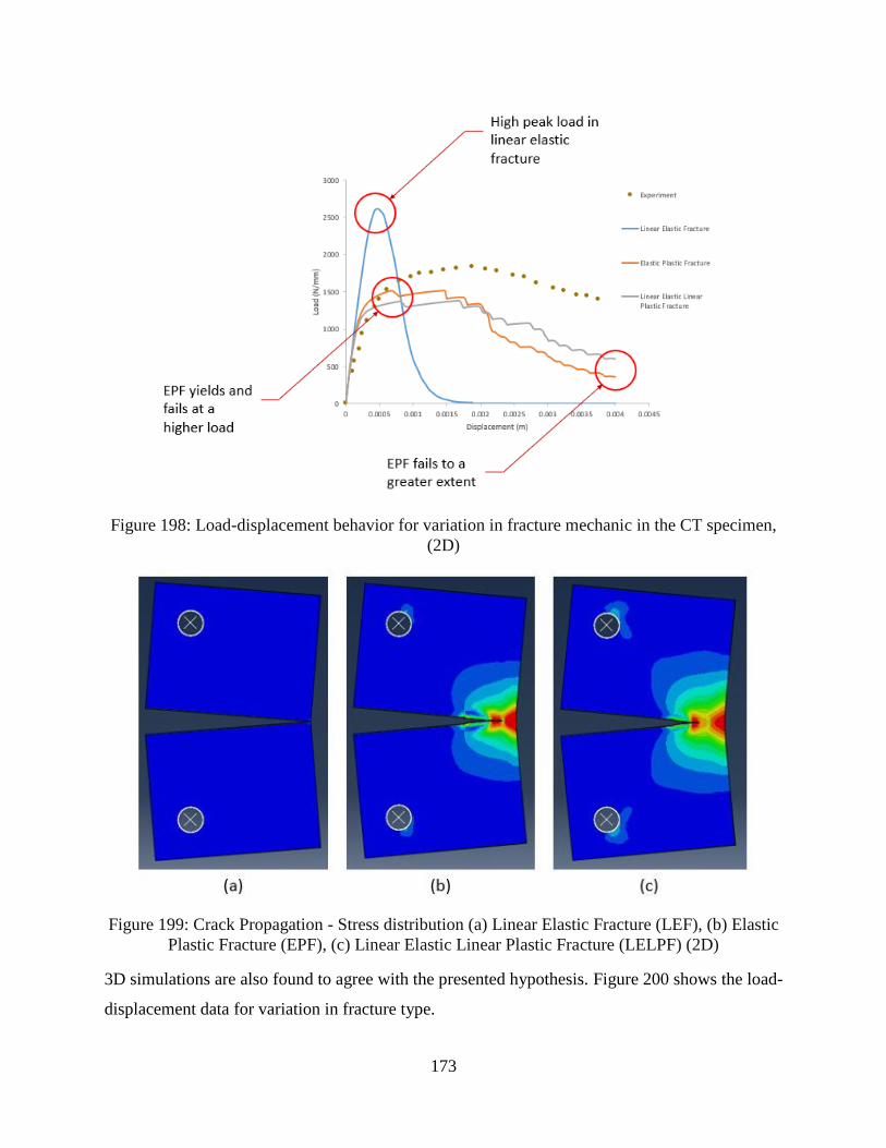
173
Figure 198: Load-displacement behavior for variation in fracture mechanic in the CT specimen,
(2D)
Figure 199: Crack Propagation - Stress distribution (a) Linear Elastic Fracture (LEF), (b) Elastic
Plastic Fracture (EPF), (c) Linear Elastic Linear Plastic Fracture (LELPF) (2D)
3D simulations are also found to agree with the presented hypothesis. Figure 200 shows the load-
displacement data for variation in fracture type.
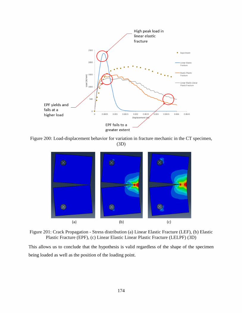
174
Figure 200: Load-displacement behavior for variation in fracture mechanic in the CT specimen,
(3D)
Figure 201: Crack Propagation - Stress distribution (a) Linear Elastic Fracture (LEF), (b) Elastic
Plastic Fracture (EPF), (c) Linear Elastic Linear Plastic Fracture (LELPF) (3D)
This allows us to conclude that the hypothesis is valid regardless of the shape of the specimen
being loaded as well as the position of the loading point.
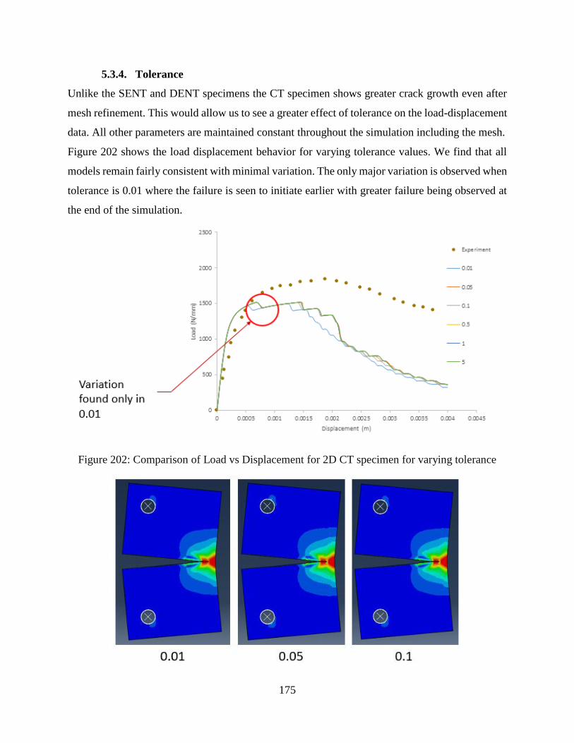
175
5.3.4. Tolerance
Unlike the SENT and DENT specimens the CT specimen shows greater crack growth even after
mesh refinement. This would allow us to see a greater effect of tolerance on the load-displacement
data. All other parameters are maintained constant throughout the simulation including the mesh.
Figure 202 shows the load displacement behavior for varying tolerance values. We find that all
models remain fairly consistent with minimal variation. The only major variation is observed when
tolerance is 0.01 where the failure is seen to initiate earlier with greater failure being observed at
the end of the simulation.
Figure 202: Comparison of Load vs Displacement for 2D CT specimen for varying tolerance
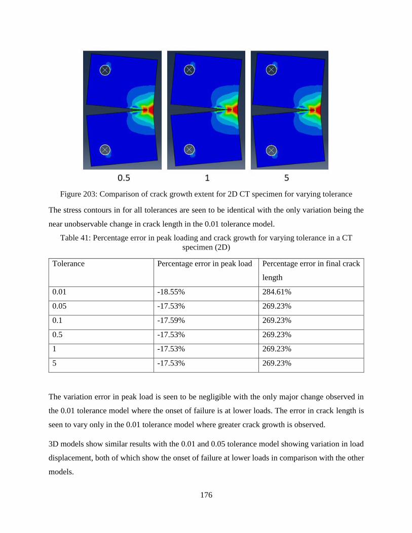
176
Figure 203: Comparison of crack growth extent for 2D CT specimen for varying tolerance
The stress contours in for all tolerances are seen to be identical with the only variation being the
near unobservable change in crack length in the 0.01 tolerance model.
Table 41: Percentage error in peak loading and crack growth for varying tolerance in a CT
specimen (2D)
Tolerance Percentage error in peak load Percentage error in final crack
length
0.01 -18.55% 284.61%
0.05 -17.53% 269.23%
0.1 -17.59% 269.23%
0.5 -17.53% 269.23%
1 -17.53% 269.23%
5 -17.53% 269.23%
The variation error in peak load is seen to be negligible with the only major change observed in
the 0.01 tolerance model where the onset of failure is at lower loads. The error in crack length is
seen to vary only in the 0.01 tolerance model where greater crack growth is observed.
3D models show similar results with the 0.01 and 0.05 tolerance model showing variation in load
displacement, both of which show the onset of failure at lower loads in comparison with the other
models.
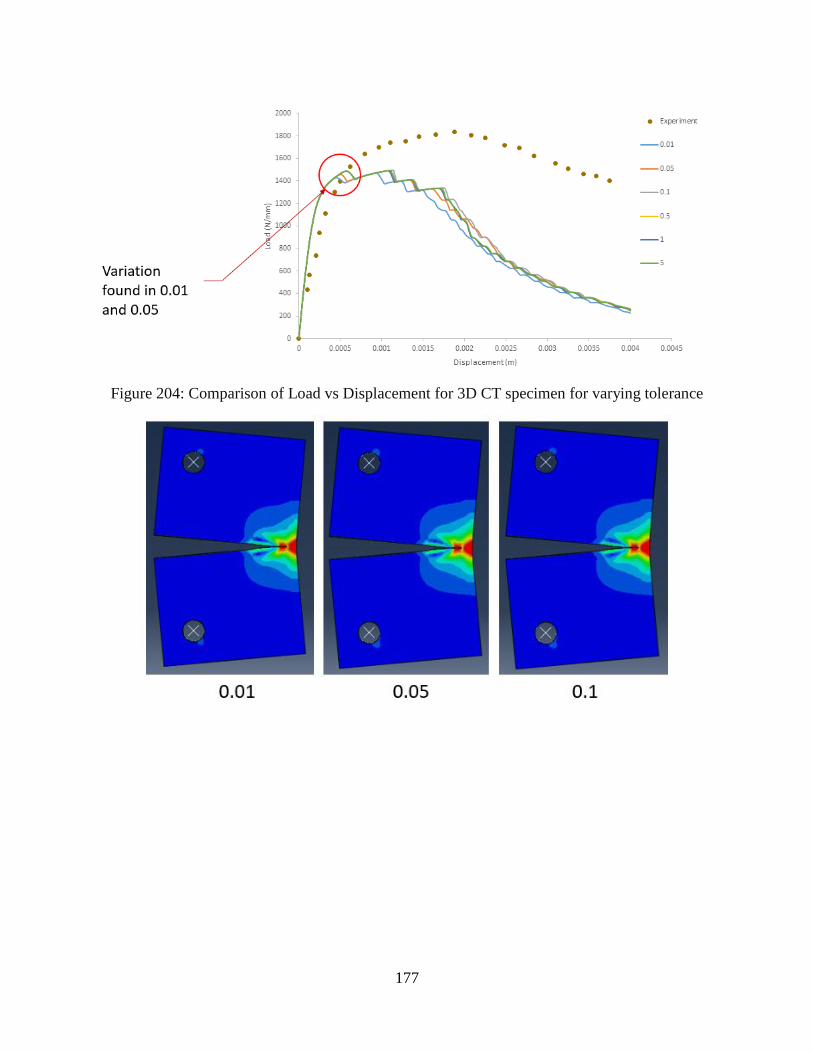
177
Figure 204: Comparison of Load vs Displacement for 3D CT specimen for varying tolerance
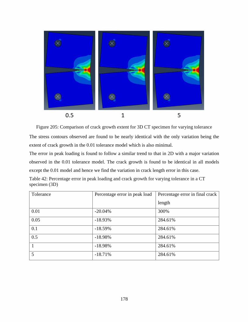
178
Figure 205: Comparison of crack growth extent for 3D CT specimen for varying tolerance
The stress contours observed are found to be nearly identical with the only variation being the
extent of crack growth in the 0.01 tolerance model which is also minimal.
The error in peak loading is found to follow a similar trend to that in 2D with a major variation
observed in the 0.01 tolerance model. The crack growth is found to be identical in all models
except the 0.01 model and hence we find the variation in crack length error in this case.
Table 42: Percentage error in peak loading and crack growth for varying tolerance in a CT
specimen (3D)
Tolerance Percentage error in peak load Percentage error in final crack
length
0.01 -20.04% 300%
0.05 -18.93% 284.61%
0.1 -18.59% 284.61%
0.5 -18.98% 284.61%
1 -18.98% 284.61%
5 -18.71% 284.61%
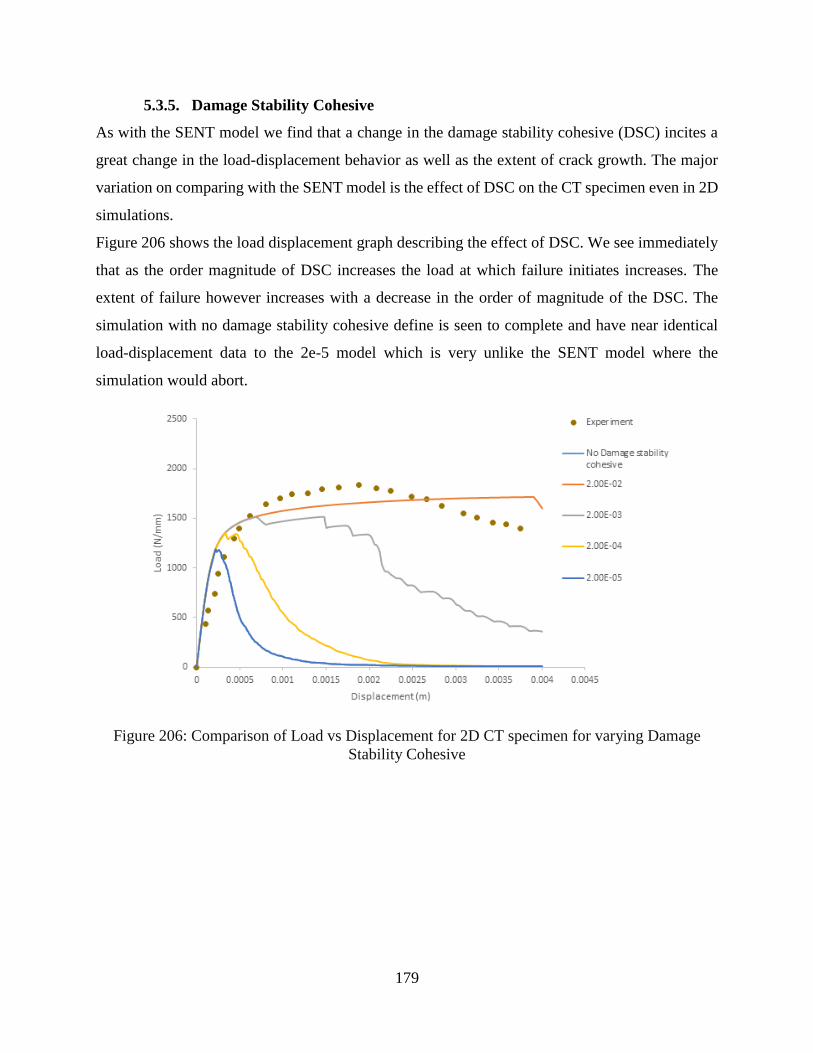
179
5.3.5. Damage Stability Cohesive
As with the SENT model we find that a change in the damage stability cohesive (DSC) incites a
great change in the load-displacement behavior as well as the extent of crack growth. The major
variation on comparing with the SENT model is the effect of DSC on the CT specimen even in 2D
simulations.
Figure 206 shows the load displacement graph describing the effect of DSC. We see immediately
that as the order magnitude of DSC increases the load at which failure initiates increases. The
extent of failure however increases with a decrease in the order of magnitude of the DSC. The
simulation with no damage stability cohesive define is seen to complete and have near identical
load-displacement data to the 2e-5 model which is very unlike the SENT model where the
simulation would abort.
Figure 206: Comparison of Load vs Displacement for 2D CT specimen for varying Damage
Stability Cohesive
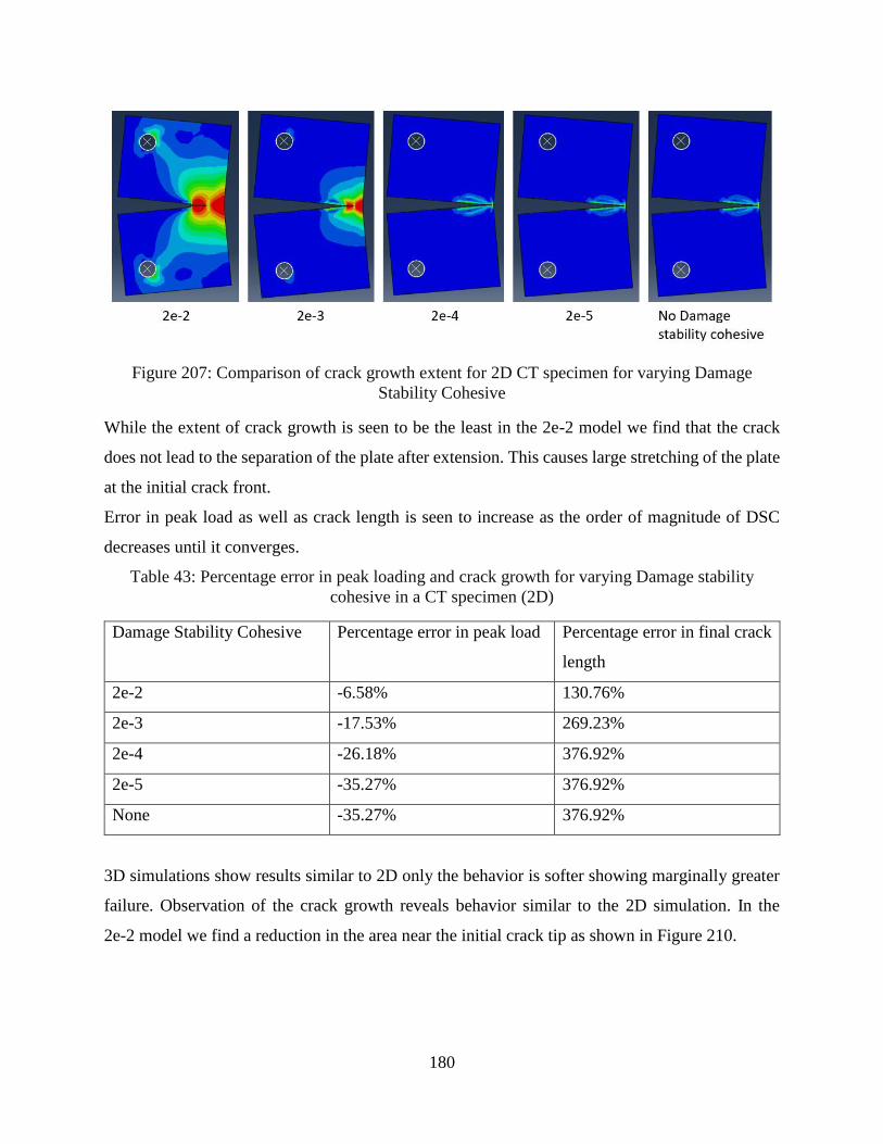
180
Figure 207: Comparison of crack growth extent for 2D CT specimen for varying Damage
Stability Cohesive
While the extent of crack growth is seen to be the least in the 2e-2 model we find that the crack
does not lead to the separation of the plate after extension. This causes large stretching of the plate
at the initial crack front.
Error in peak load as well as crack length is seen to increase as the order of magnitude of DSC
decreases until it converges.
Table 43: Percentage error in peak loading and crack growth for varying Damage stability
cohesive in a CT specimen (2D)
Damage Stability Cohesive Percentage error in peak load Percentage error in final crack
length
2e-2 -6.58% 130.76%
2e-3 -17.53% 269.23%
2e-4 -26.18% 376.92%
2e-5 -35.27% 376.92%
None -35.27% 376.92%
3D simulations show results similar to 2D only the behavior is softer showing marginally greater
failure. Observation of the crack growth reveals behavior similar to the 2D simulation. In the
2e-2 model we find a reduction in the area near the initial crack tip as shown in Figure 210.
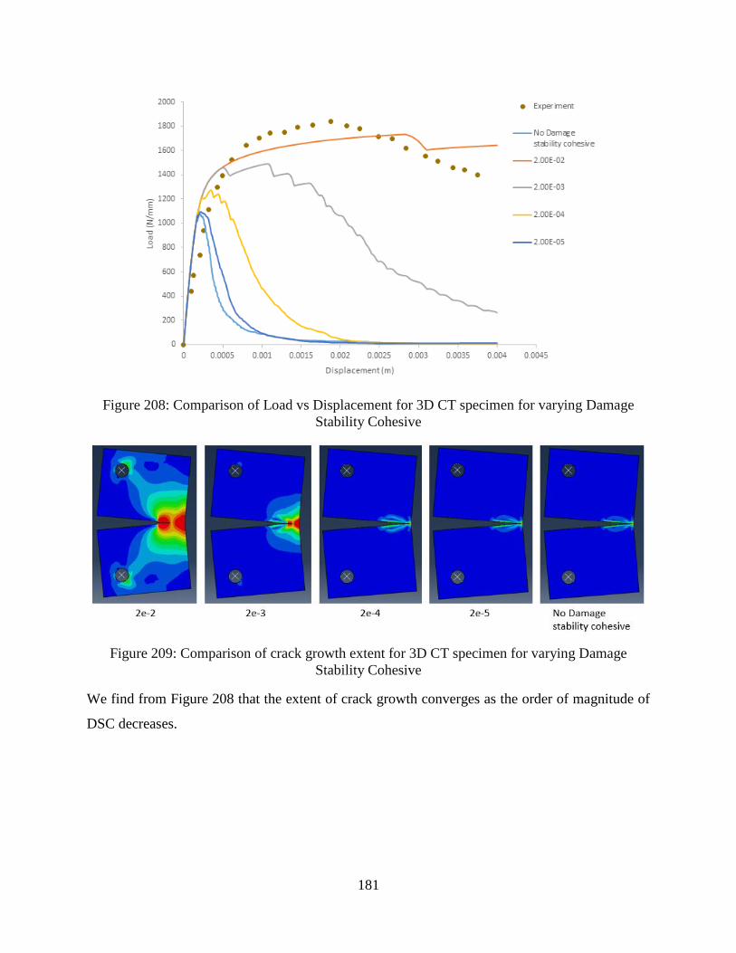
181
Figure 208: Comparison of Load vs Displacement for 3D CT specimen for varying Damage
Stability Cohesive
Figure 209: Comparison of crack growth extent for 3D CT specimen for varying Damage
Stability Cohesive
We find from Figure 208 that the extent of crack growth converges as the order of magnitude of
DSC decreases.
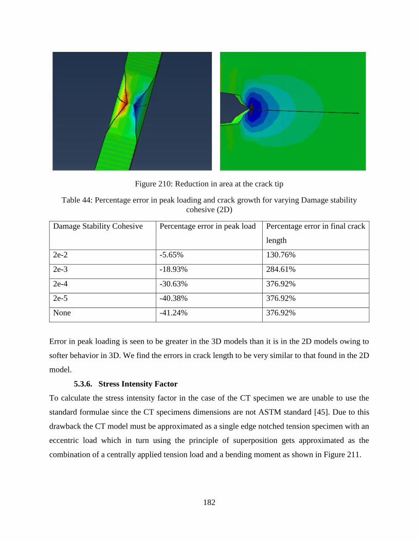
182
Figure 210: Reduction in area at the crack tip
Table 44: Percentage error in peak loading and crack growth for varying Damage stability
cohesive (2D)
Damage Stability Cohesive Percentage error in peak load Percentage error in final crack
length
2e-2 -5.65% 130.76%
2e-3 -18.93% 284.61%
2e-4 -30.63% 376.92%
2e-5 -40.38% 376.92%
None -41.24% 376.92%
Error in peak loading is seen to be greater in the 3D models than it is in the 2D models owing to
softer behavior in 3D. We find the errors in crack length to be very similar to that found in the 2D
model.
5.3.6. Stress Intensity Factor
To calculate the stress intensity factor in the case of the CT specimen we are unable to use the
standard formulae since the CT specimens dimensions are not ASTM standard [45]. Due to this
drawback the CT model must be approximated as a single edge notched tension specimen with an
eccentric load which in turn using the principle of superposition gets approximated as the
combination of a centrally applied tension load and a bending moment as shown in Figure 211.
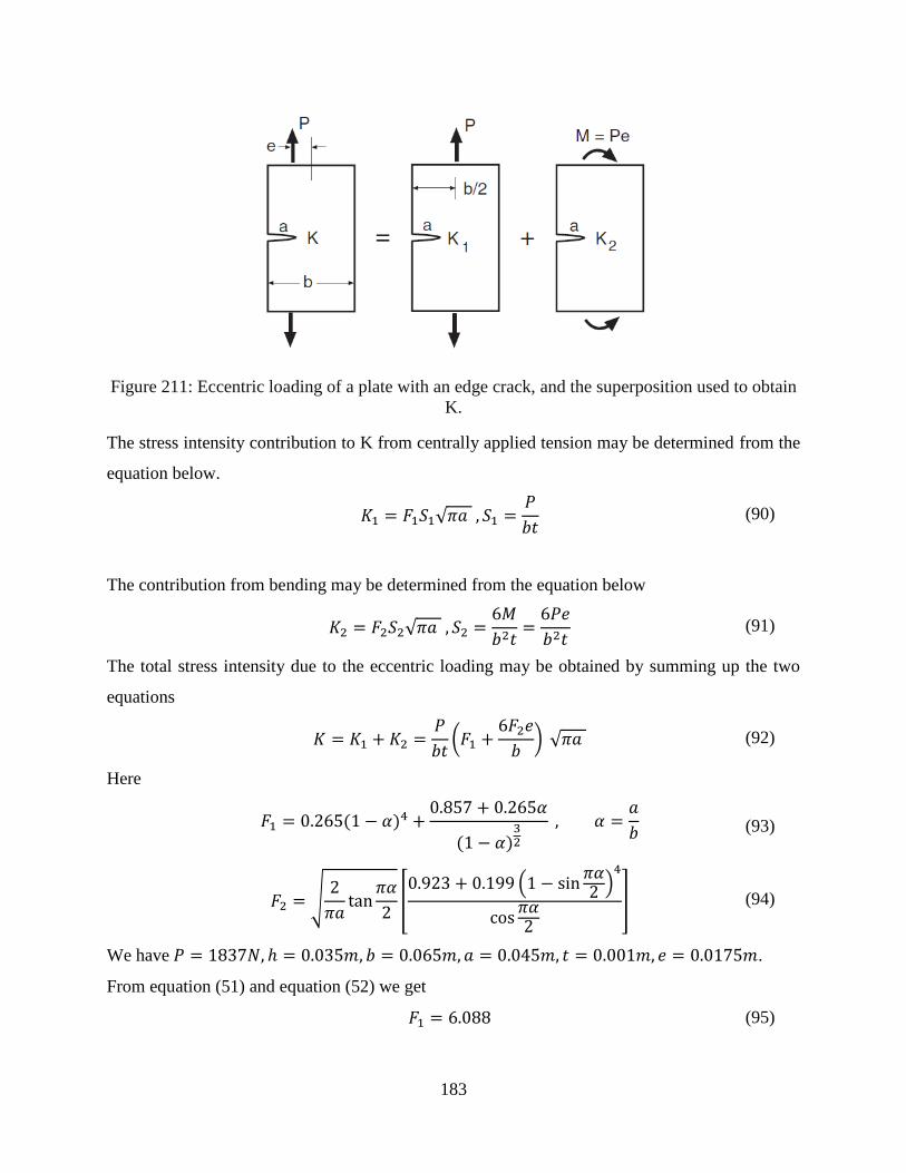
183
Figure 211: Eccentric loading of a plate with an edge crack, and the superposition used to obtain
K.
The stress intensity contribution to K from centrally applied tension may be determined from the
equation below.
𝐾1 = 𝐹1𝑆1√𝜋𝑎 , 𝑆1 =𝑃
𝑏𝑡 (90)
The contribution from bending may be determined from the equation below
𝐾2 = 𝐹2𝑆2√𝜋𝑎 , 𝑆2 =6𝑀
𝑏2𝑡=
6𝑃𝑒
𝑏2𝑡 (91)
The total stress intensity due to the eccentric loading may be obtained by summing up the two
equations
𝐾 = 𝐾1 + 𝐾2 =𝑃
𝑏𝑡(𝐹1 +
6𝐹2𝑒
𝑏) √𝜋𝑎 (92)
Here
𝐹1 = 0.265(1 − 𝛼)4 +0.857 + 0.265𝛼
(1 − 𝛼)32
, 𝛼 =𝑎
𝑏 (93)
𝐹2 = √2
𝜋𝑎tan
𝜋𝛼
2[0.923 + 0.199 (1 − sin
𝜋𝛼2 )
4
cos𝜋𝛼2
] (94)
We have 𝑃 = 1837𝑁, ℎ = 0.035𝑚, 𝑏 = 0.065𝑚, 𝑎 = 0.045𝑚, 𝑡 = 0.001𝑚, 𝑒 = 0.0175𝑚.
From equation (51) and equation (52) we get
𝐹1 = 6.088 (95)
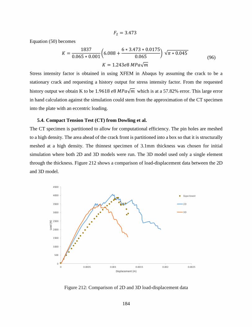
184
𝐹2 = 3.473
Equation (50) becomes
𝐾 =
1837
0.065 ∗ 0.001(6.088 +
6 ∗ 3.473 ∗ 0.0175
0.065) √𝜋 ∗ 0.045
𝐾 = 1.243𝑒8 𝑀𝑃𝑎√𝑚
(96)
Stress intensity factor is obtained in using XFEM in Abaqus by assuming the crack to be a
stationary crack and requesting a history output for stress intensity factor. From the requested
history output we obtain K to be 1.9618 𝑒8 𝑀𝑃𝑎√𝑚 which is at a 57.82% error. This large error
in hand calculation against the simulation could stem from the approximation of the CT specimen
into the plate with an eccentric loading.
5.4. Compact Tension Test (CT) from Dowling et al.
The CT specimen is partitioned to allow for computational efficiency. The pin holes are meshed
to a high density. The area ahead of the crack front is partitioned into a box so that it is structurally
meshed at a high density. The thinnest specimen of 3.1mm thickness was chosen for initial
simulation where both 2D and 3D models were run. The 3D model used only a single element
through the thickness. Figure 212 shows a comparison of load-displacement data between the 2D
and 3D model.
Figure 212: Comparison of 2D and 3D load-displacement data
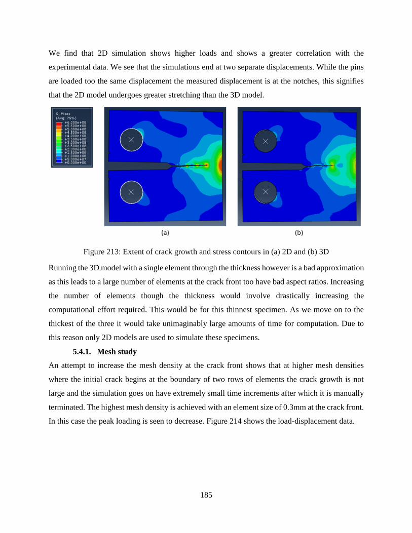
185
We find that 2D simulation shows higher loads and shows a greater correlation with the
experimental data. We see that the simulations end at two separate displacements. While the pins
are loaded too the same displacement the measured displacement is at the notches, this signifies
that the 2D model undergoes greater stretching than the 3D model.
Figure 213: Extent of crack growth and stress contours in (a) 2D and (b) 3D
Running the 3D model with a single element through the thickness however is a bad approximation
as this leads to a large number of elements at the crack front too have bad aspect ratios. Increasing
the number of elements though the thickness would involve drastically increasing the
computational effort required. This would be for this thinnest specimen. As we move on to the
thickest of the three it would take unimaginably large amounts of time for computation. Due to
this reason only 2D models are used to simulate these specimens.
5.4.1. Mesh study
An attempt to increase the mesh density at the crack front shows that at higher mesh densities
where the initial crack begins at the boundary of two rows of elements the crack growth is not
large and the simulation goes on have extremely small time increments after which it is manually
terminated. The highest mesh density is achieved with an element size of 0.3mm at the crack front.
In this case the peak loading is seen to decrease. Figure 214 shows the load-displacement data.
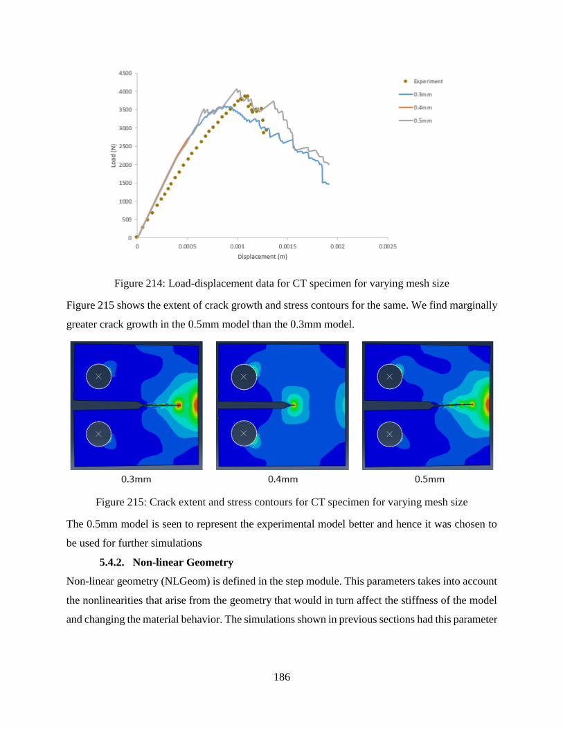
186
Figure 214: Load-displacement data for CT specimen for varying mesh size
Figure 215 shows the extent of crack growth and stress contours for the same. We find marginally
greater crack growth in the 0.5mm model than the 0.3mm model.
Figure 215: Crack extent and stress contours for CT specimen for varying mesh size
The 0.5mm model is seen to represent the experimental model better and hence it was chosen to
be used for further simulations
5.4.2. Non-linear Geometry
Non-linear geometry (NLGeom) is defined in the step module. This parameters takes into account
the nonlinearities that arise from the geometry that would in turn affect the stiffness of the model
and changing the material behavior. The simulations shown in previous sections had this parameter
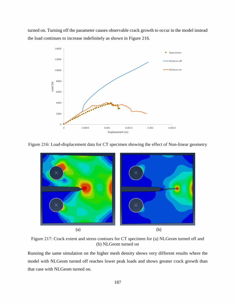
187
turned on. Turning off the parameter causes observable crack growth to occur in the model instead
the load continues to increase indefinitely as shown in Figure 216.
Figure 216: Load-displacement data for CT specimen showing the effect of Non-linear geometry
Figure 217: Crack extent and stress contours for CT specimen for (a) NLGeom turned off and
(b) NLGeom turned on
Running the same simulation on the higher mesh density shows very different results where the
model with NLGeom turned off reaches lower peak loads and shows greater crack growth than
that case with NLGeom turned on.
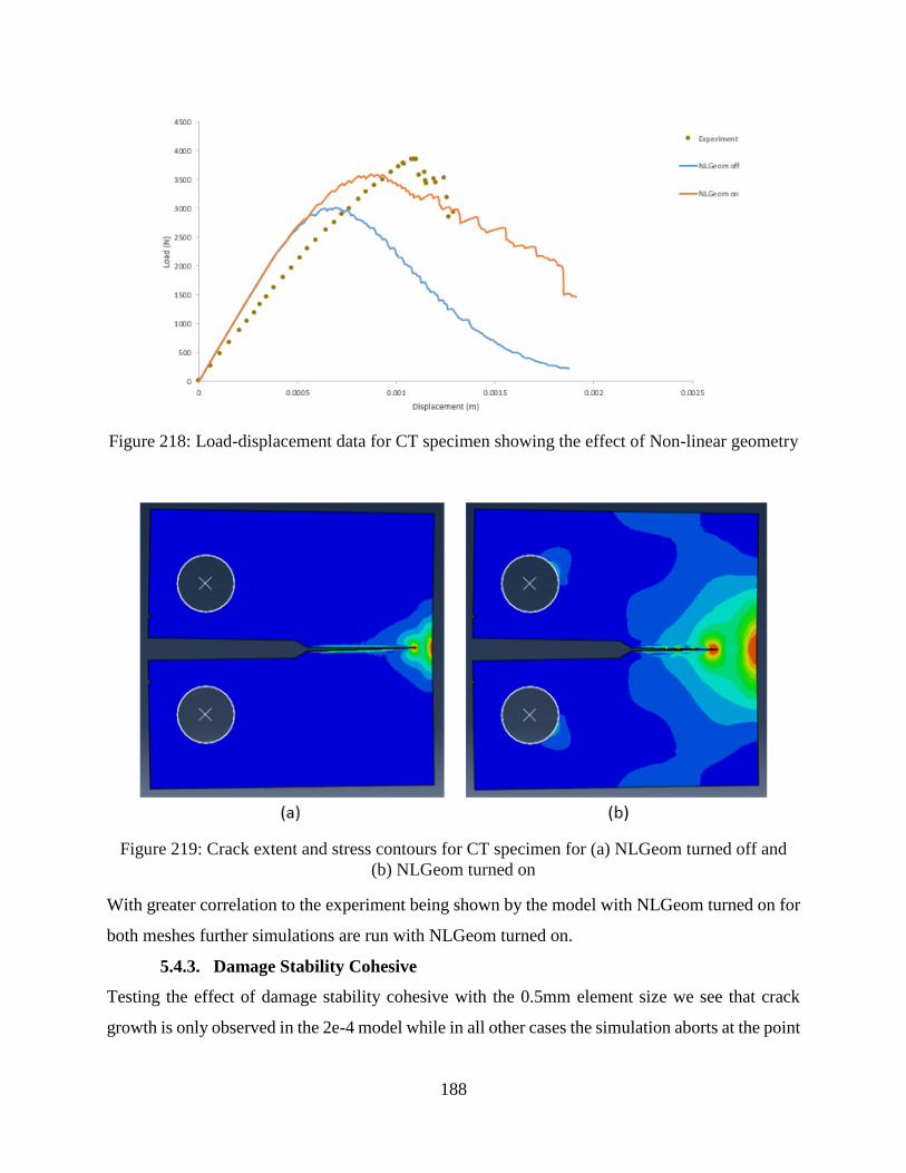
188
Figure 218: Load-displacement data for CT specimen showing the effect of Non-linear geometry
Figure 219: Crack extent and stress contours for CT specimen for (a) NLGeom turned off and
(b) NLGeom turned on
With greater correlation to the experiment being shown by the model with NLGeom turned on for
both meshes further simulations are run with NLGeom turned on.
5.4.3. Damage Stability Cohesive
Testing the effect of damage stability cohesive with the 0.5mm element size we see that crack
growth is only observed in the 2e-4 model while in all other cases the simulation aborts at the point
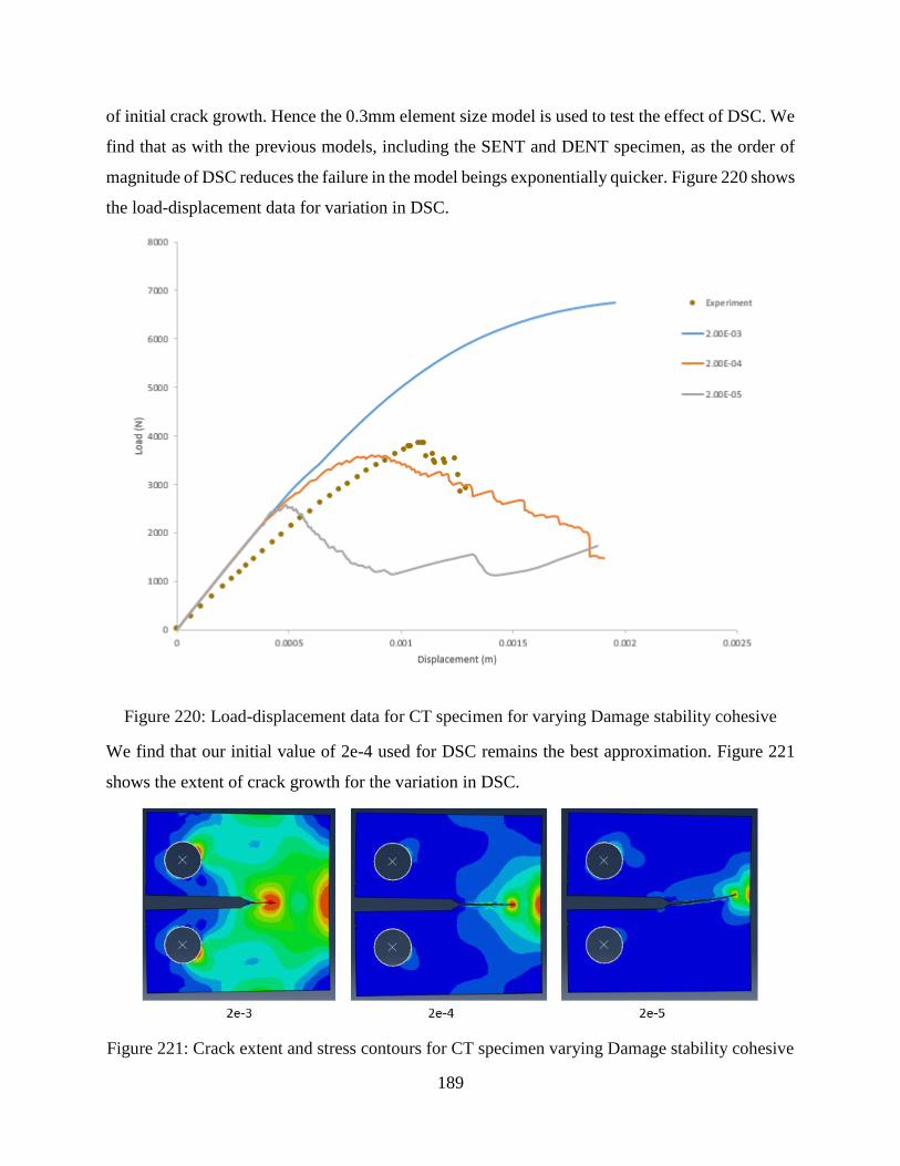
189
of initial crack growth. Hence the 0.3mm element size model is used to test the effect of DSC. We
find that as with the previous models, including the SENT and DENT specimen, as the order of
magnitude of DSC reduces the failure in the model beings exponentially quicker. Figure 220 shows
the load-displacement data for variation in DSC.
Figure 220: Load-displacement data for CT specimen for varying Damage stability cohesive
We find that our initial value of 2e-4 used for DSC remains the best approximation. Figure 221
shows the extent of crack growth for the variation in DSC.
Figure 221: Crack extent and stress contours for CT specimen varying Damage stability cohesive
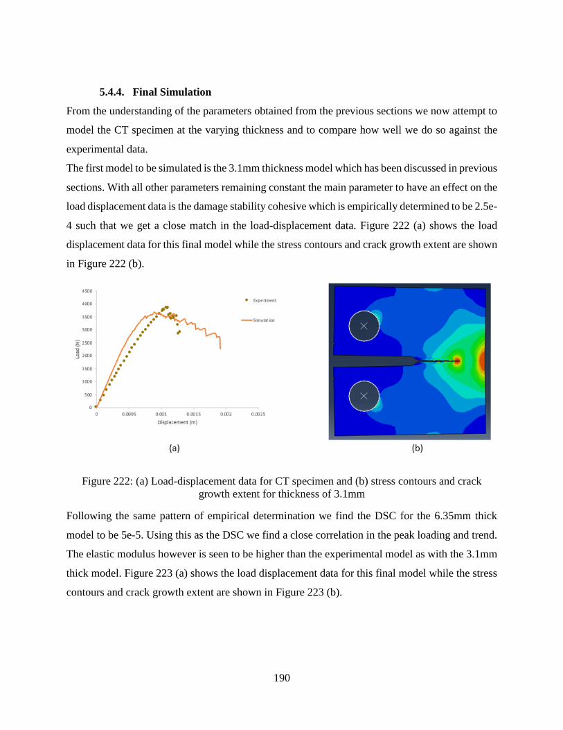
190
5.4.4. Final Simulation
From the understanding of the parameters obtained from the previous sections we now attempt to
model the CT specimen at the varying thickness and to compare how well we do so against the
experimental data.
The first model to be simulated is the 3.1mm thickness model which has been discussed in previous
sections. With all other parameters remaining constant the main parameter to have an effect on the
load displacement data is the damage stability cohesive which is empirically determined to be 2.5e-
4 such that we get a close match in the load-displacement data. Figure 222 (a) shows the load
displacement data for this final model while the stress contours and crack growth extent are shown
in Figure 222 (b).
Figure 222: (a) Load-displacement data for CT specimen and (b) stress contours and crack
growth extent for thickness of 3.1mm
Following the same pattern of empirical determination we find the DSC for the 6.35mm thick
model to be 5e-5. Using this as the DSC we find a close correlation in the peak loading and trend.
The elastic modulus however is seen to be higher than the experimental model as with the 3.1mm
thick model. Figure 223 (a) shows the load displacement data for this final model while the stress
contours and crack growth extent are shown in Figure 223 (b).
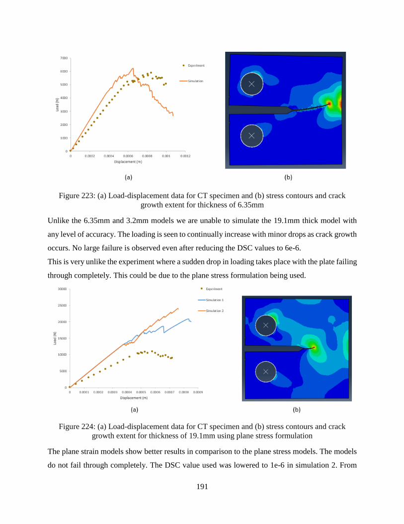
191
Figure 223: (a) Load-displacement data for CT specimen and (b) stress contours and crack
growth extent for thickness of 6.35mm
Unlike the 6.35mm and 3.2mm models we are unable to simulate the 19.1mm thick model with
any level of accuracy. The loading is seen to continually increase with minor drops as crack growth
occurs. No large failure is observed even after reducing the DSC values to 6e-6.
This is very unlike the experiment where a sudden drop in loading takes place with the plate failing
through completely. This could be due to the plane stress formulation being used.
Figure 224: (a) Load-displacement data for CT specimen and (b) stress contours and crack
growth extent for thickness of 19.1mm using plane stress formulation
The plane strain models show better results in comparison to the plane stress models. The models
do not fail through completely. The DSC value used was lowered to 1e-6 in simulation 2. From
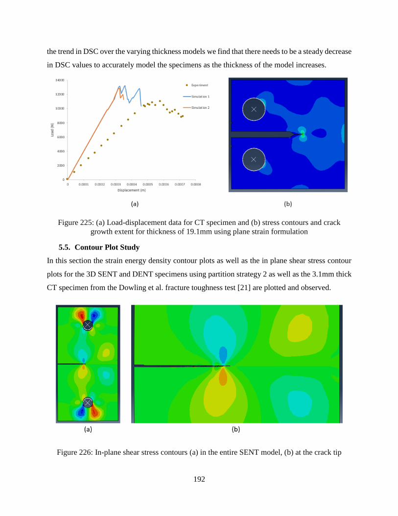
192
the trend in DSC over the varying thickness models we find that there needs to be a steady decrease
in DSC values to accurately model the specimens as the thickness of the model increases.
Figure 225: (a) Load-displacement data for CT specimen and (b) stress contours and crack
growth extent for thickness of 19.1mm using plane strain formulation
5.5. Contour Plot Study
In this section the strain energy density contour plots as well as the in plane shear stress contour
plots for the 3D SENT and DENT specimens using partition strategy 2 as well as the 3.1mm thick
CT specimen from the Dowling et al. fracture toughness test [21] are plotted and observed.
Figure 226: In-plane shear stress contours (a) in the entire SENT model, (b) at the crack tip
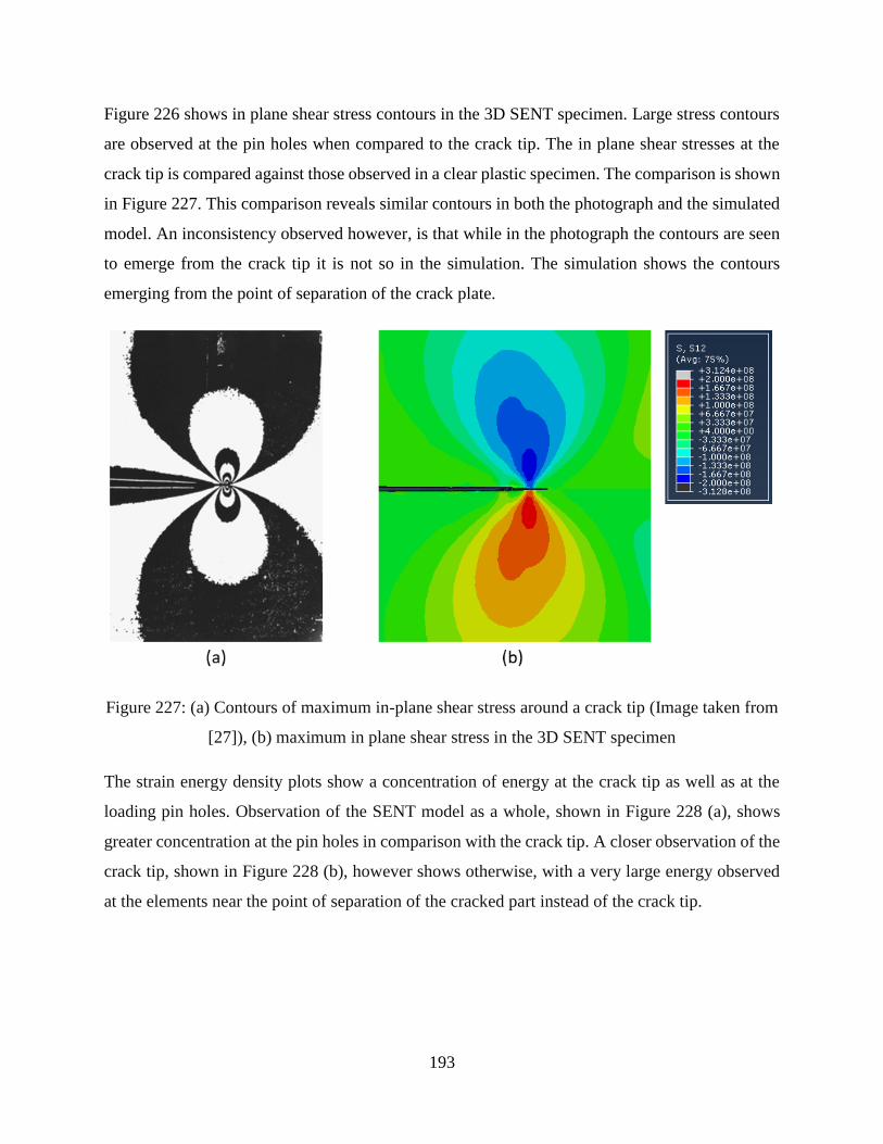
193
Figure 226 shows in plane shear stress contours in the 3D SENT specimen. Large stress contours
are observed at the pin holes when compared to the crack tip. The in plane shear stresses at the
crack tip is compared against those observed in a clear plastic specimen. The comparison is shown
in Figure 227. This comparison reveals similar contours in both the photograph and the simulated
model. An inconsistency observed however, is that while in the photograph the contours are seen
to emerge from the crack tip it is not so in the simulation. The simulation shows the contours
emerging from the point of separation of the crack plate.
Figure 227: (a) Contours of maximum in-plane shear stress around a crack tip (Image taken from
[27]), (b) maximum in plane shear stress in the 3D SENT specimen
The strain energy density plots show a concentration of energy at the crack tip as well as at the
loading pin holes. Observation of the SENT model as a whole, shown in Figure 228 (a), shows
greater concentration at the pin holes in comparison with the crack tip. A closer observation of the
crack tip, shown in Figure 228 (b), however shows otherwise, with a very large energy observed
at the elements near the point of separation of the cracked part instead of the crack tip.
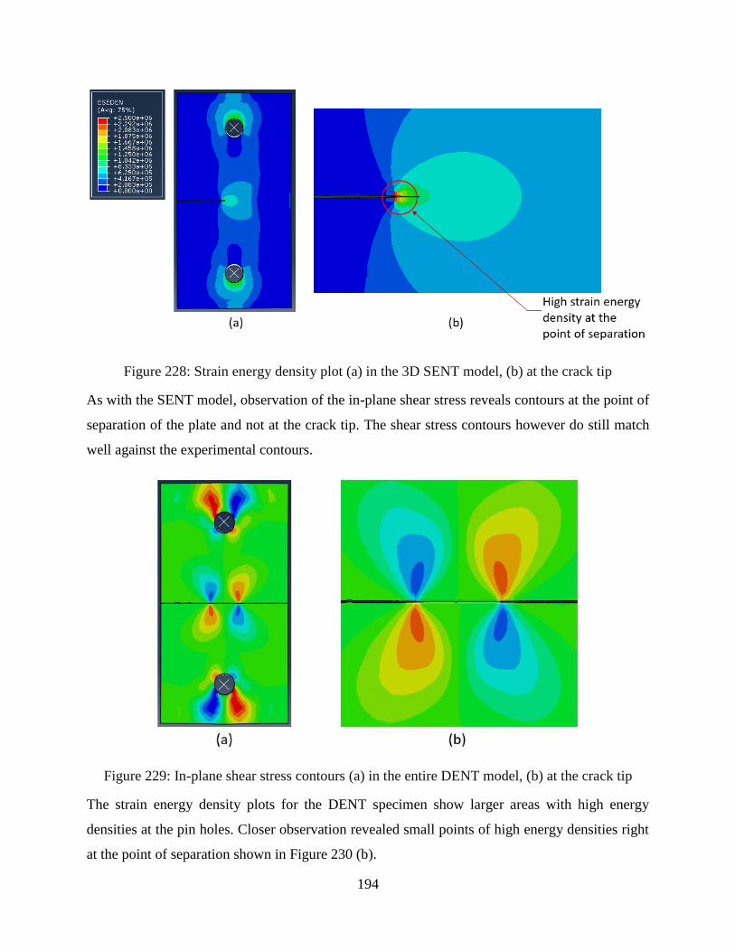
194
Figure 228: Strain energy density plot (a) in the 3D SENT model, (b) at the crack tip
As with the SENT model, observation of the in-plane shear stress reveals contours at the point of
separation of the plate and not at the crack tip. The shear stress contours however do still match
well against the experimental contours.
Figure 229: In-plane shear stress contours (a) in the entire DENT model, (b) at the crack tip
The strain energy density plots for the DENT specimen show larger areas with high energy
densities at the pin holes. Closer observation revealed small points of high energy densities right
at the point of separation shown in Figure 230 (b).
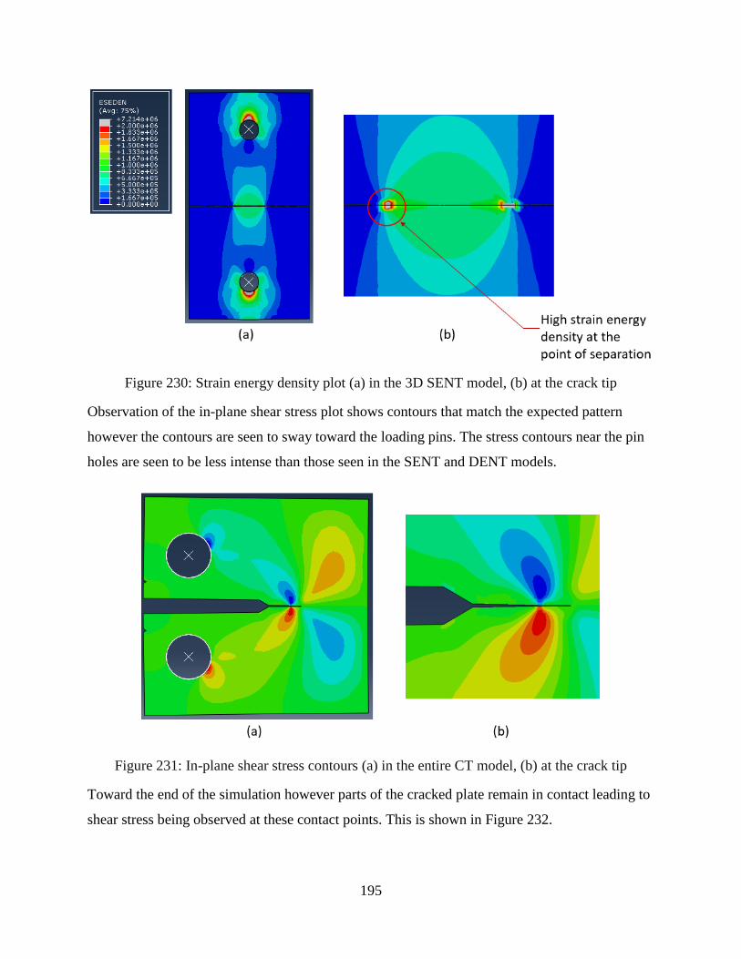
195
Figure 230: Strain energy density plot (a) in the 3D SENT model, (b) at the crack tip
Observation of the in-plane shear stress plot shows contours that match the expected pattern
however the contours are seen to sway toward the loading pins. The stress contours near the pin
holes are seen to be less intense than those seen in the SENT and DENT models.
Figure 231: In-plane shear stress contours (a) in the entire CT model, (b) at the crack tip
Toward the end of the simulation however parts of the cracked plate remain in contact leading to
shear stress being observed at these contact points. This is shown in Figure 232.
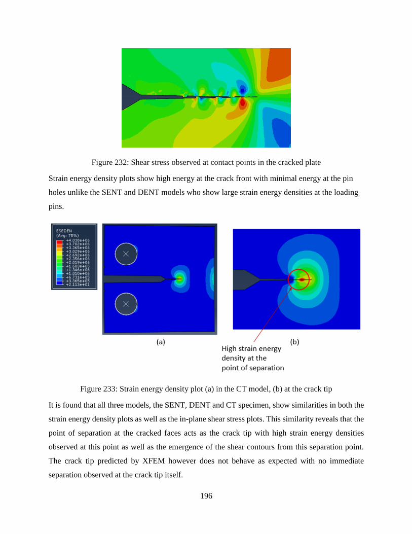
196
Figure 232: Shear stress observed at contact points in the cracked plate
Strain energy density plots show high energy at the crack front with minimal energy at the pin
holes unlike the SENT and DENT models who show large strain energy densities at the loading
pins.
Figure 233: Strain energy density plot (a) in the CT model, (b) at the crack tip
It is found that all three models, the SENT, DENT and CT specimen, show similarities in both the
strain energy density plots as well as the in-plane shear stress plots. This similarity reveals that the
point of separation at the cracked faces acts as the crack tip with high strain energy densities
observed at this point as well as the emergence of the shear contours from this separation point.
The crack tip predicted by XFEM however does not behave as expected with no immediate
separation observed at the crack tip itself.
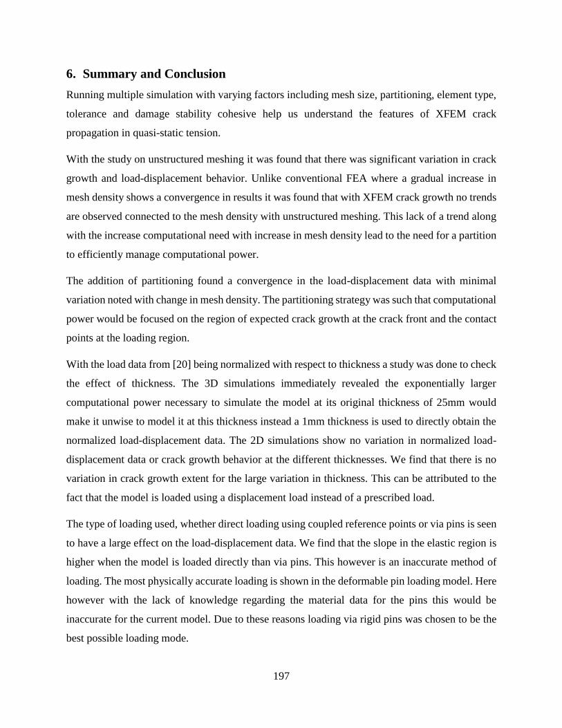
197
6. Summary and Conclusion
Running multiple simulation with varying factors including mesh size, partitioning, element type,
tolerance and damage stability cohesive help us understand the features of XFEM crack
propagation in quasi-static tension.
With the study on unstructured meshing it was found that there was significant variation in crack
growth and load-displacement behavior. Unlike conventional FEA where a gradual increase in
mesh density shows a convergence in results it was found that with XFEM crack growth no trends
are observed connected to the mesh density with unstructured meshing. This lack of a trend along
with the increase computational need with increase in mesh density lead to the need for a partition
to efficiently manage computational power.
The addition of partitioning found a convergence in the load-displacement data with minimal
variation noted with change in mesh density. The partitioning strategy was such that computational
power would be focused on the region of expected crack growth at the crack front and the contact
points at the loading region.
With the load data from [20] being normalized with respect to thickness a study was done to check
the effect of thickness. The 3D simulations immediately revealed the exponentially larger
computational power necessary to simulate the model at its original thickness of 25mm would
make it unwise to model it at this thickness instead a 1mm thickness is used to directly obtain the
normalized load-displacement data. The 2D simulations show no variation in normalized load-
displacement data or crack growth behavior at the different thicknesses. We find that there is no
variation in crack growth extent for the large variation in thickness. This can be attributed to the
fact that the model is loaded using a displacement load instead of a prescribed load.
The type of loading used, whether direct loading using coupled reference points or via pins is seen
to have a large effect on the load-displacement data. We find that the slope in the elastic region is
higher when the model is loaded directly than via pins. This however is an inaccurate method of
loading. The most physically accurate loading is shown in the deformable pin loading model. Here
however with the lack of knowledge regarding the material data for the pins this would be
inaccurate for the current model. Due to these reasons loading via rigid pins was chosen to be the
best possible loading mode.
198
A hypothesis regarding the load displacement behavior is made based on the plasticity of the
material defined. The hypothesis made states that for two models having the same parameters in
all aspects except the plasticity, the model having elastic plastic fracture is found to yield at a
higher load and fail earlier than a model with linear-elastic linear plastic fracture. This hypothesis
is seen to hold across all the models thereby confirming it.
The next parameter that was studied is the tolerance. The tolerance is found to be a necessary
parameter to allow for crack growth in the model. While no major effect is noticed in the SENT
and CT models based on the tolerance the DENT model shows a large variation with tolerance. It
is found that as the tolerance reduces the failure in the model increases, the tolerance is also seen
to affect how early failure is initiated in the model. This effect is seen to a small extent in the CT
model where at the lowest tolerance we do see failure occurring earlier than the remaining models.
Damage stability cohesive (DSC) is a parameter that is seen to affect all models in the same pattern.
The order of magnitude of DSC is seen to directly affect the extent of failure in the model as well
as how early failure initiates in the model. As the order of magnitude of the DSC reduces we find
that failure in the model initiates quicker and the extent of failure is greater. This parameter as well
as the tolerance only effects the load displacement behavior after yield. None of the tested
parameters are seen to have any effect on the load displacement behavior in the elastic region. In
the SENT and the DENT model we find that the simulation shows a lower elastic modulus while
in the CT models both the [20] as well as the [21] models we find that the elastic modulus is seen
to be higher.
Based on the understanding obtained from CT specimens, specimens provided in [21] are modeled.
It is found that by varying the DSC it is possible to make the model fail at the same load as the
experiment however we are unable to change the behavior in the elastic region without directly
varying the material properties. In the experimental setup the load displacement data is abruptly
stopped at the point where the crack causes the entire specimen to fail and split apart. In
comparison it was found that the simulated model never fails through completely for the same
extensometer displacement. Comparing the behavior of all the models it is found that the CT
specimens provided in [20] and [21] are the most accurately modelled. While there is still a
discrepancy in the elastic region it is possible sufficiently modify behavior in the plastic region to
get a close match to the experimental results.
199
Studies on the strain energy density plots and the in-plane shear stress show unexpected behavior
in the contours. Large strain energy densities are observed point of separation of the crack while
it is expected to be at the crack tip. The in-plane shear stresses also reveal contours that are
experimentally observed at the crack tip are being projected at the point of separation instead.
These observations remain consistent through all the models that are simulated. From these
observations it can be inferred that the point of separation of the plate as the crack passes through
acts effectively as the crack tip.
Certain models in the simulation show a trend in loading where upon reaching a peak load it
plateaus out while other models show a drop in load after reaching the peak. This is caused due to
the partitioning of the plate which leads to a more converged mesh which in turn shows a plateau
in the loading. This is also only seen in the SENT and DENT specimen whereas in the CT specimen
we see that even on mesh refinement there is no such plateaus observed. This effect in the loading
graph is a function of the shape and loading type on the specimen.
7. Contributions and Future work
Attempts were made to understand the features of XFEM. Lack of experimental details to create
fully representative models existed in all the models, however we gain an understanding of how
XFEM causes the simulations to behave. An understanding into the need for partitioning and
structural meshing to converge solutions based on XFEM is made. The variation in an
unstructured, unpartitioned mesh is found to be excessive for varying mesh sizes with larger
computational requirements at higher mesh densities. An increased mesh density at the crack front,
preferably a structured mesh with a high mesh density at contact points is found to be the optimal
meshing strategy for XFEM crack growth. A dependence on type of loading mechanism is observe
with loading via pins showing lower elastic modulus than in a case with directly coupled loading.
Normalized loading data can be used to reduce computational efficiency by reducing the thickness
of the model to unity. This reduction in thickness provides the same normalized load-displacement
data with minimal variation. The downside to using a unity thickness model in 3D is that we lose
resolution of crack growth through the thickness.
The hypothesis provided regarding the load-displacement behavior in elastic plastic fracture and
linear elastic linear plastic fracture would allow us to make an approximate prediction of the

200
behavior of a Ramberg-Osgood model based on its behavior using linear elastic linear plastic
fracture. The plastic zone predictions based on von Mises criterion and Tresca criterion are
confirmed at the crack front in the XFEM simulations.
Tolerance is seen to affect the crack growth in the models at lower magnitudes with the failure
increasing as the magnitude of tolerance reduces. The damage stability cohesive is seen to have a
much more visible effect on the model with similar effects to tolerance. As the DSC reduces in
order of magnitude the failure of the model is seen to increase drastically. This parameter helps us
significantly to model failure accurately with respect to the experimental model. XFEM however
is seen to have a major drawback in the elastic region with no parameter other than the material
properties having an effect on the load-displacement data in the elastic region. It is found that in
the SENT and DENT specimens the elastic modulus appears lower than the experimental data
while in the CT models, both in the [20] model as well as the [21] model, the appearance of a
higher elastic modulus is observed.
A deeper study into the underlying formulation of XFEM in Abaqus could be conducted. This
would help us gain a better understanding into the reason for inaccuracy during loading in the
elastic region. Subsequently, similar study could be conducted on more complicated specimens to
verify the applicability of the XFEM formulation for a wide range of scenarios. Persistent residual
stresses observed in the XFEM solutions even after separation of the top and bottom halves of the
DENT model further demand an in depth study to be conducted to discover the reasons for this
inaccuracy.
201
References
[1] R. Claudio, R. Baptista, V. Infante and C. Branco, "Life Prediction Using Finite Elements in
Complex Geometries," 8AS Jorndas De Fractura, pp. 203-211, 2002.
[2] American Society for Testing and Materials, "Annual Book of ASTM Standards," ASTM, 2003.
[3] A. Hrennikoff, "Solution of problems of elasticity by the framework method," Journal of applied
mechanics, p. 169–175, 1941.
[4] R. Courant, "Variational methods for the solution of problems of equilibrium and vibrations,"
Bulletin of the American Mathematical Society, p. 1–23, 1943.
[5] L. N. Trefethen and D. Bau, III, Numerical Linear Algebra, SIAM, 1997.
[6] S. Binnamangala and J. Bayandor, "Numerical Analysis of Dynamically Loaded Advanced
Stiffened Aerospace Composite Structures with Bonded/Fastened Joints," in 49th AIAA Aerospace
Sciences Meeting including the New Horizons Forum and Aerospace Exposition, Orlando, 2011.
[7] T. L. Anderson, Fracture Mechanics: Fundamentals and Applications, Boca Raton: CRC Press,
2005.
[8] N. Moës, J. Dolbow and T. Belytschko, "A finite element method for crack growth without
remeshing," International Journal for Numerical Methods in Engineering, vol. 46, no. 1, p. 131–
150, 1999.
[9] Z. Zhuang, Z. L. Cheng and J. Liao, Extended Finite Element Analysis, Beijing: Tsinghua
University Press, 2014.
[10] P. Behroozinia, R. Mirzaeifar and J. Bayandor, "Numerical Investigation of Scale Factor in
Composites Applying Extended Finite Element Method," in AIAA Modeling and Simulation
Technologies Conference , San Diego, 2016.
[11] G. Vigueras, F. Sket, C. Samaniego, L. Wu, L. Noels, D. Tjahjanto, E. Casoni, G. Houzeaux, A.
Makradi, J. M. Molina-Aldareguia, M. Vázquez and A. Jérusalem, "An XFEM/CZM
implementation for massively parallel simulations of composites fracture," Composite Structures,
vol. 125, pp. 542-557, 2015.
[12] A. C. Orifici, R. S. Thomson, R. Degenhardt, C. Bisagni and J. Bayandor, "Development of a finite-
element analysis methodology for the propagation of delaminations in composite structures,"
Mechanics of Composite Materials, vol. 43, no. 1, pp. 9-28, 2007.
[13] S. Shah, J. Bayandor, F. Abdi and A. Najafi, "Micro Mechanics based Prognosis of Progressive
Dynamic Damage in Advanced Aerospace Composite Structures," in International Congress of the
Aeronautical Sciences, 2010.
202
[14] T. Nagashima and H. Suemasu, "X-FEM analyses of a thin-walled composite shell structure with a
delamination," Computers & Structures, vol. 88, no. 9-10, pp. 549-557, 2010.
[15] H. W. Wang, H. W. Zhou, H. W. Ji and X. C. Zhang, "Application of extended finite element
method in damage progress simulation of fiber reinforced composites," Materials & Design, vol.
55, pp. 191-196, 2014.
[16] G. Yi, T. Yu, T. Quoc Bui, C. Ma and S. Hirose, "SIFs evaluation of sharp V-notched fracture by
XFEM and strain energy approach," Theoretical and Applied Fracture Mechanics, vol. 89, pp. 35-
44, 2017.
[17] J.-Y. Wu and F.-B. Li, "An improved stable XFEM (Is-XFEM) with a novel enrichment function
for the computational modeling of cohesive cracks," Computer Methods in Applied Mechanics and
Engineering, vol. 295, pp. 77-107, 2015.
[18] L. Wen and R. Tian, "Improved XFEM: Accurate and robust dynamic crack growth simulation,"
Computer Methods in Applied Mechanics and Engineering, vol. 308, pp. 256-285, 2016.
[19] Dassault Systemes, Abaqus 6.12 Online Documentation, Providence, Rhode Island,, 2012.
[20] L. Xia, C. Shih and J. W. Hutchinson, "A computational approach to ductile crack growth under
large scale yielding conditions," Journal of the Mechanics and Physics of Solids, vol. 43, no. 3, pp.
389-413, 1995.
[21] N. Dowling, D. Reed, K. Tontodonato and M. McCord, "Fracture Toughness test," Blacksburg,
2013.
[22] S. Timoshenko and J. N. Goodier, Theory of Elasticity, Stanford: McGraw-Hill, 1951.
[23] A. A. Griffith, "The phenomena of rupture and flow in solids," Philosophical Transactions of the
Royal Society of London, vol. A, no. 221, p. 163–198, 1921.
[24] "Wikipedia," [Online]. Available: https://en.wikipedia.org/wiki/Fracture_mechanics.
[25] E. Orowan, "Fracture and Strength of Solids," Reports On Progress in Physics, vol. 12, pp. 185-
232, 1949.
[26] G. R. Irwin, "Analysis of stresses and strains near the end of a crack traversing a plate," Journal of
Applied Mechanics, vol. 24, pp. 361-364, 1957.
[27] N. E. Dowling, Mechanical Behaviour of Materials, Fourth ed., Pearson, 2013.
[28] efunda, "efunda," 2017. [Online]. Available:
http://www.efunda.com/formulae/solid_mechanics/fracture_mechanics/fm_epfm_CTOD.cfm.
[29] G. R. Irwin and J. A. Kies, "Critical energy rate analysis of fracture strength," Welding Journal
Research Supplement, vol. 33, p. 193s–198s, 1954.
[30] ASTM Special Committee on Fracture Testing of High, ASTM Bulletin, pp. 29-40, 1960.
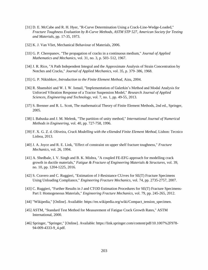
203
[31] D. E. McCabe and R. H. Hyer, "R-Curve Determination Using a Crack-Line-Wedge-Loaded,"
Fracture Toughness Evaluation by R-Curve Methods, ASTM STP 527, American Society for Testing
and Materials, pp. 17-35, 1973.
[32] K. J. Van Vliet, Mechanical Behaviour of Materials, 2006.
[33] G. P. Cherepanov, "The propagation of cracks in a continuous medium," Journal of Applied
Mathematics and Mechanics, vol. 31, no. 3, p. 503–512, 1967.
[34] J. R. Rice, "A Path Independent Integral and the Approximate Analysis of Strain Concentration by
Notches and Cracks," Journal of Applied Mechanics, vol. 35, p. 379–386, 1968.
[35] G. P. Nikishkov, Introduction to the Finite Element Method, Aizu, 2004.
[36] R. Shamshiri and W. I. W. Ismail, "Implementation of Galerkin’s Method and Modal Analysis for
Unforced Vibration Response of a Tractor Suspension Model," Research Journal of Applied
Sciences, Engineering and Technology, vol. 7, no. 1, pp. 49-55, 2013.
[37] S. Brenner and R. L. Scott, The mathematical Theory of Finite Element Methods, 2nd ed., Springer,
2005.
[38] I. Babuska and J. M. Melenk, "The partition of unity method," International Journal of Numerical
Methods in Engineering, vol. 40, pp. 727-758, 1996.
[39] F. X. G. Z. d. Oliveira, Crack Modelling with the eXtended Finite Element Method, Lisbon: Tecnico
Lisboa, 2013.
[40] J. A. Joyce and R. E. Link, "Effect of constraint on upper shelf fracture toughness," Fracture
Mechanics, vol. 26, 1994.
[41] A. Shedbale, I. V. Singh and B. K. Mishra, "A coupled FE-EFG approach for modelling crack
growth in ductile materials," Fatigue & Fracture of Engineering Materials & Structures, vol. 39,
no. 10, pp. 1204-1225, 2016.
[42] S. Cravero and C. Ruggieri, "Estimation of J-Resistance CUrves for SE(T) Fracture Specimens
Using Unloading Compliance," Engineering Fracture Mechanics, vol. 74, pp. 2735-2757, 2007.
[43] C. Ruggieri, "Further Results in J and CTOD Estimation Procedures for SE(T) Fracture Specimens-
Part I: Homogeneous Materials," Engineering Fracture Mechanics, vol. 79, pp. 245-265, 2012.
[44] "Wikipedia," [Online]. Available: https://en.wikipedia.org/wiki/Compact_tension_specimen.
[45] ASTM, "Standard Test Method for Measurement of Fatigue Crack Growth Rates," ASTM
International, 2000.
[46] Springer, "Springer," [Online]. Available: https://link.springer.com/content/pdf/10.1007%2F978-
94-009-4333-9_4.pdf.
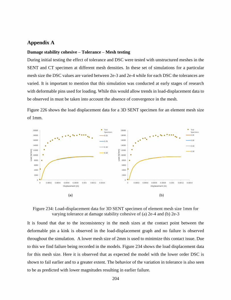
204
Appendix A
Damage stability cohesive – Tolerance – Mesh testing
During initial testing the effect of tolerance and DSC were tested with unstructured meshes in the
SENT and CT specimen at different mesh densities. In these set of simulations for a particular
mesh size the DSC values are varied between 2e-3 and 2e-4 while for each DSC the tolerances are
varied. It is important to mention that this simulation was conducted at early stages of research
with deformable pins used for loading. While this would allow trends in load-displacement data to
be observed in must be taken into account the absence of convergence in the mesh.
Figure 226 shows the load displacement data for a 3D SENT specimen for an element mesh size
of 1mm.
Figure 234: Load-displacement data for 3D SENT specimen of element mesh size 1mm for
varying tolerance at damage stability cohesive of (a) 2e-4 and (b) 2e-3
It is found that due to the inconsistency in the mesh sizes at the contact point between the
deformable pin a kink is observed in the load-displacement graph and no failure is observed
throughout the simulation. A lower mesh size of 2mm is used to minimize this contact issue. Due
to this we find failure being recorded in the models. Figure 234 shows the load displacement data
for this mesh size. Here it is observed that as expected the model with the lower order DSC is
shown to fail earlier and to a greater extent. The behavior of the variation in tolerance is also seen
to be as predicted with lower magnitudes resulting in earlier failure.
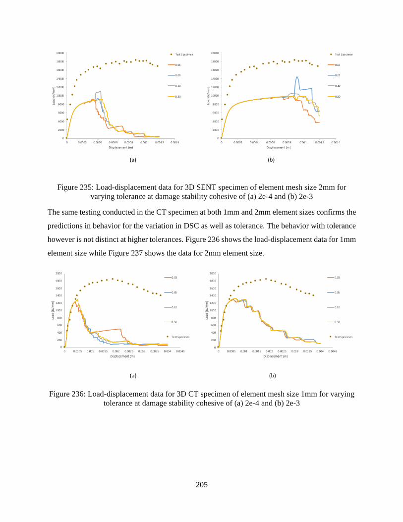
205
Figure 235: Load-displacement data for 3D SENT specimen of element mesh size 2mm for
varying tolerance at damage stability cohesive of (a) 2e-4 and (b) 2e-3
The same testing conducted in the CT specimen at both 1mm and 2mm element sizes confirms the
predictions in behavior for the variation in DSC as well as tolerance. The behavior with tolerance
however is not distinct at higher tolerances. Figure 236 shows the load-displacement data for 1mm
element size while Figure 237 shows the data for 2mm element size.
Figure 236: Load-displacement data for 3D CT specimen of element mesh size 1mm for varying
tolerance at damage stability cohesive of (a) 2e-4 and (b) 2e-3
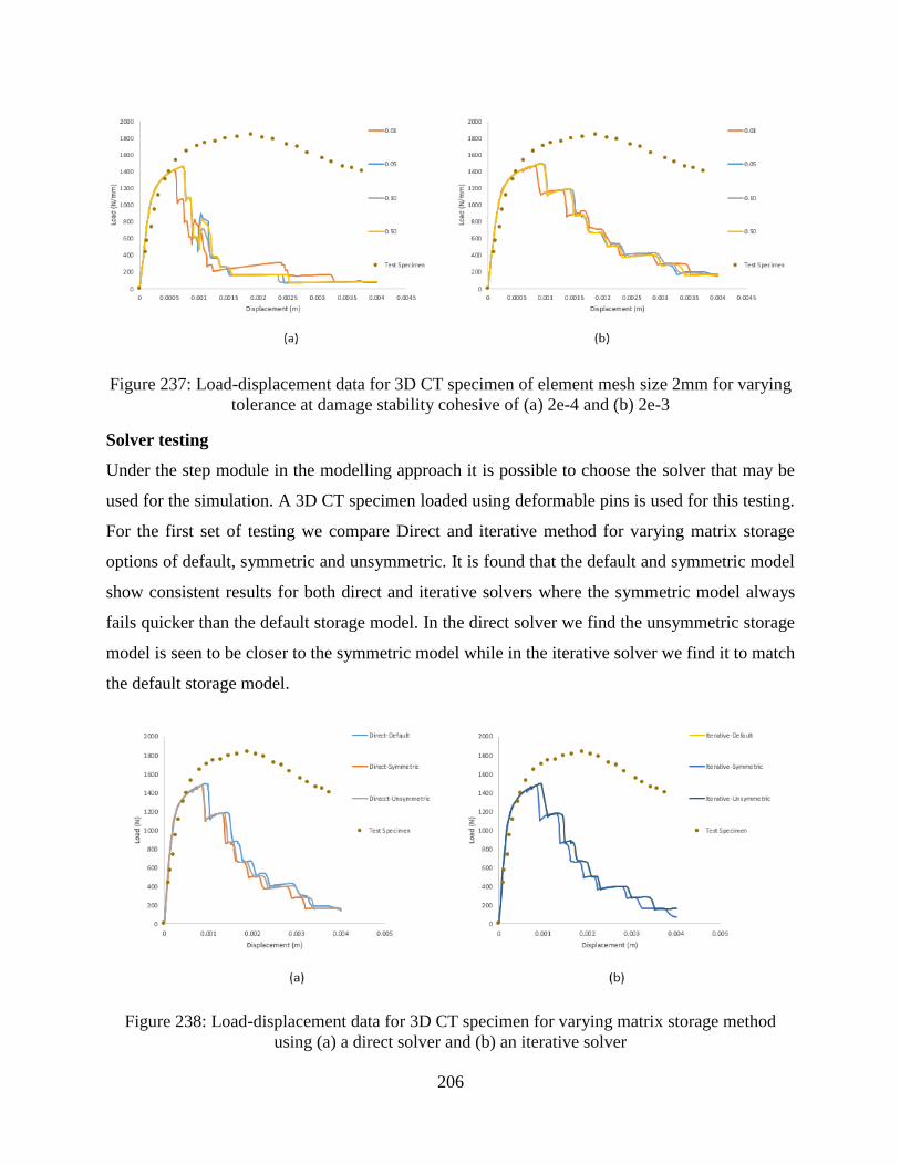
206
Figure 237: Load-displacement data for 3D CT specimen of element mesh size 2mm for varying
tolerance at damage stability cohesive of (a) 2e-4 and (b) 2e-3
Solver testing
Under the step module in the modelling approach it is possible to choose the solver that may be
used for the simulation. A 3D CT specimen loaded using deformable pins is used for this testing.
For the first set of testing we compare Direct and iterative method for varying matrix storage
options of default, symmetric and unsymmetric. It is found that the default and symmetric model
show consistent results for both direct and iterative solvers where the symmetric model always
fails quicker than the default storage model. In the direct solver we find the unsymmetric storage
model is seen to be closer to the symmetric model while in the iterative solver we find it to match
the default storage model.
Figure 238: Load-displacement data for 3D CT specimen for varying matrix storage method
using (a) a direct solver and (b) an iterative solver
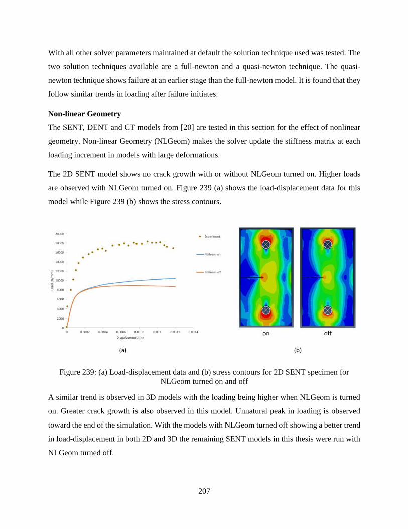
207
With all other solver parameters maintained at default the solution technique used was tested. The
two solution techniques available are a full-newton and a quasi-newton technique. The quasi-
newton technique shows failure at an earlier stage than the full-newton model. It is found that they
follow similar trends in loading after failure initiates.
Non-linear Geometry
The SENT, DENT and CT models from [20] are tested in this section for the effect of nonlinear
geometry. Non-linear Geometry (NLGeom) makes the solver update the stiffness matrix at each
loading increment in models with large deformations.
The 2D SENT model shows no crack growth with or without NLGeom turned on. Higher loads
are observed with NLGeom turned on. Figure 239 (a) shows the load-displacement data for this
model while Figure 239 (b) shows the stress contours.
Figure 239: (a) Load-displacement data and (b) stress contours for 2D SENT specimen for
NLGeom turned on and off
A similar trend is observed in 3D models with the loading being higher when NLGeom is turned
on. Greater crack growth is also observed in this model. Unnatural peak in loading is observed
toward the end of the simulation. With the models with NLGeom turned off showing a better trend
in load-displacement in both 2D and 3D the remaining SENT models in this thesis were run with
NLGeom turned off.
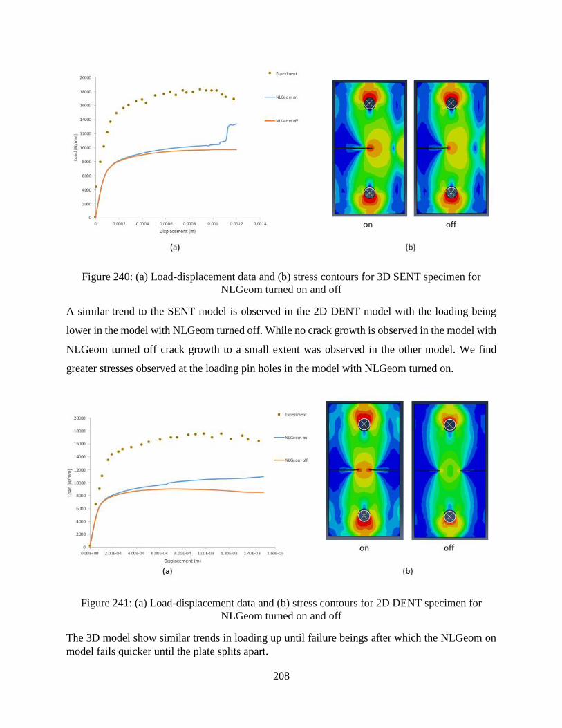
208
Figure 240: (a) Load-displacement data and (b) stress contours for 3D SENT specimen for
NLGeom turned on and off
A similar trend to the SENT model is observed in the 2D DENT model with the loading being
lower in the model with NLGeom turned off. While no crack growth is observed in the model with
NLGeom turned off crack growth to a small extent was observed in the other model. We find
greater stresses observed at the loading pin holes in the model with NLGeom turned on.
Figure 241: (a) Load-displacement data and (b) stress contours for 2D DENT specimen for
NLGeom turned on and off
The 3D model show similar trends in loading up until failure beings after which the NLGeom on
model fails quicker until the plate splits apart.
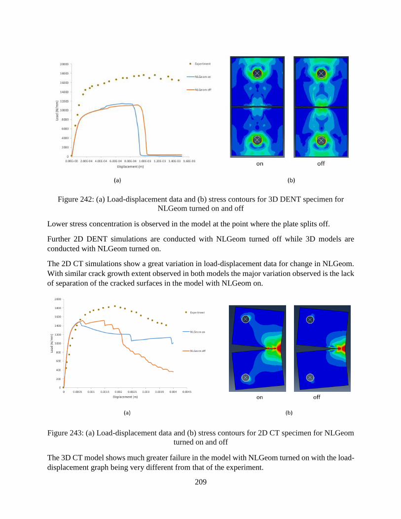
209
Figure 242: (a) Load-displacement data and (b) stress contours for 3D DENT specimen for
NLGeom turned on and off
Lower stress concentration is observed in the model at the point where the plate splits off.
Further 2D DENT simulations are conducted with NLGeom turned off while 3D models are
conducted with NLGeom turned on.
The 2D CT simulations show a great variation in load-displacement data for change in NLGeom.
With similar crack growth extent observed in both models the major variation observed is the lack
of separation of the cracked surfaces in the model with NLGeom on.
Figure 243: (a) Load-displacement data and (b) stress contours for 2D CT specimen for NLGeom
turned on and off
The 3D CT model shows much greater failure in the model with NLGeom turned on with the load-
displacement graph being very different from that of the experiment.
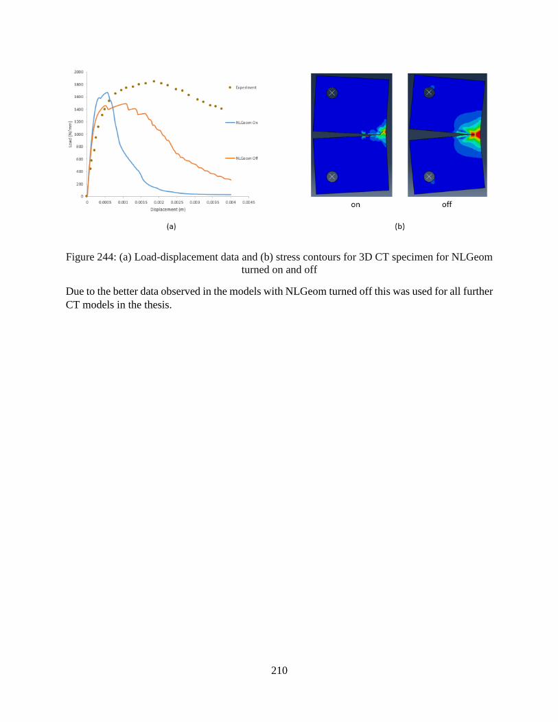
210
Figure 244: (a) Load-displacement data and (b) stress contours for 3D CT specimen for NLGeom
turned on and off
Due to the better data observed in the models with NLGeom turned off this was used for all further
CT models in the thesis.