Crack propagation with the XFEM and a hybrid explicit ... · PDF fileCrack propagation with the XFEM and a hybrid explicit-implicit crack description T.P. Fries and M. Baydoun May,

Crack propagation with the XFEM and a hybrid

explicit-implicit crack description

T.P. Fries and M. Baydoun

May, 2011

Abstract

A method for two and three dimensional crack propagation is presented which

combines the advantages of explicit and implicit crack descriptions. An implicit de-

scription in the frame of the level-set method is advantageous for the simulation within

the extended finite element method (XFEM). The XFEM has proven its potential in

fracture mechanics as it provides accurate solutions without any remeshing during the

crack simulation. On the other hand, an explicit representation of the crack, e.g. by

means of a polyhedron, enables a simple update of the crack during the propagation.

A key aspect in the proposed method is the introduction of three level-set functions

that are computed exactly from the explicit representation. These functions imply a

coordinate system at the crack front and serve as a basis for the enrichment. Fur-

thermore, a simple model for the crack propagation is presented. One of the biggest

achievements of the proposed method is that two and three-dimensional crack simu-

lations are treated in a consistent manner. That is, the extension from two to three

dimensions is truly straightforward.

2 CONTENTS

Contents

1 Introduction 4

2 XFEM approximations in fracture mechanics 7

3 Explicit description of cracks 8

3.1 Explicit description of cracks in two dimensions . . . . . . . . . . . . . . . 8

3.1.1 Definition of the crack path . . . . . . . . . . . . . . . . . . . . . . 8

3.1.2 Normal vectors on the crack path . . . . . . . . . . . . . . . . . . . 9

3.1.3 Definition of the crack tip(s) . . . . . . . . . . . . . . . . . . . . . . 9

3.1.4 Coordinate system at the crack tip(s) . . . . . . . . . . . . . . . . . 10

3.1.5 Extension of the crack path . . . . . . . . . . . . . . . . . . . . . . 10

3.1.6 Limitations . . . . . . . . . . . . . . . . . . . . . . . . . . . . . . . 11

3.2 Explicit description of cracks in three dimensions . . . . . . . . . . . . . . 11

3.2.1 Definition of the crack surface . . . . . . . . . . . . . . . . . . . . . 11

3.2.2 Normal vectors on the crack surface . . . . . . . . . . . . . . . . . . 12

3.2.3 Definition of the crack front . . . . . . . . . . . . . . . . . . . . . . 12

3.2.4 Coordinate system at the crack front . . . . . . . . . . . . . . . . . 13

3.2.5 Extension of the crack surface . . . . . . . . . . . . . . . . . . . . . 14

3.2.6 Limitations . . . . . . . . . . . . . . . . . . . . . . . . . . . . . . . 14

4 Definition of level-set functions 15

4.1 The level-set functions in two dimensions . . . . . . . . . . . . . . . . . . . 16

4.2 The level-set functions in three dimensions . . . . . . . . . . . . . . . . . . 17

4.3 Discretization of the level-set functions . . . . . . . . . . . . . . . . . . . . 19

CONTENTS 3

5 Coordinate systems implied by the level-set functions 21

5.1 The coordinate system (r, θ) . . . . . . . . . . . . . . . . . . . . . . . . . . 21

5.2 The coordinate system (a, b) . . . . . . . . . . . . . . . . . . . . . . . . . . 22

5.3 The set of enriched nodes . . . . . . . . . . . . . . . . . . . . . . . . . . . 23

5.4 The enrichment functions . . . . . . . . . . . . . . . . . . . . . . . . . . . 25

6 Crack propagation 27

6.1 The crack increment . . . . . . . . . . . . . . . . . . . . . . . . . . . . . . 28

6.2 Update of the crack path/surface . . . . . . . . . . . . . . . . . . . . . . . 31

6.3 Update of the extended crack path/surface . . . . . . . . . . . . . . . . . . 31

7 Numerical results 32

7.1 Crack propagation in two dimensions . . . . . . . . . . . . . . . . . . . . . 33

7.1.1 Tension and shearing in a unit-square specimen . . . . . . . . . . . 33

7.1.2 Asymmetric bending of a beam . . . . . . . . . . . . . . . . . . . . 35

7.1.3 Splitting test case of a circular domain . . . . . . . . . . . . . . . . 36

7.1.4 One edge crack in a specimen with holes . . . . . . . . . . . . . . . 39

7.1.5 Two cracks in a specimen with holes . . . . . . . . . . . . . . . . . 41

7.2 Crack propagation in three dimensions . . . . . . . . . . . . . . . . . . . . 42

7.2.1 Pseudo-three-dimensional bending beam . . . . . . . . . . . . . . . 42

7.2.2 Prismatic beam under torsion . . . . . . . . . . . . . . . . . . . . . 44

7.2.3 Plate under impact . . . . . . . . . . . . . . . . . . . . . . . . . . . 44

8 Conclusions 46

References 48

4 Introduction

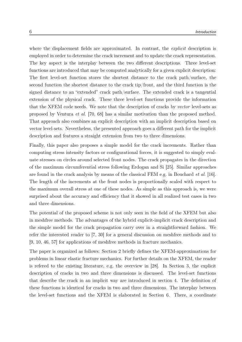
1 Introduction

The extended finite element method (XFEM) enables the accurate approximation of fields

that involve jumps, kinks, singularities, and other non-smooth features within elements

[6, 49, 28]. This is achieved by adding additional terms—the enrichments—to classical

finite element approximations. These terms enable the approximation to capture the non-

smooth features independently of the mesh. The XFEM has shown its full potential for

applications in fracture mechanics, see e.g. Karihaloo [45]. Applications with cracks involve

discontinuities across the crack surface and singularities (or general steep gradients) at the

crack front. In the classical FEM, a suitable mesh has to be provided and maintained which

accounts for these features [1, 42]; this is particularly difficult for crack propagation in three

dimensions. The XFEM, however, can treat these type of problems on fixed meshes and

considers for crack propagation by a dynamic enrichment of the approximation. For recent

developments in the XFEM, the reader is refered to the special issue in [31]; an overview

on the XFEM is given in Fries and Belytschko [28].

In the context of the XFEM, the location of the non-smooth features are often defined

implicitly by means of the level-set method, see e.g. Osher et al. [52, 51] and Bloomenthal

et al. [14]. The extension of the level-set method to the description of crack paths in two

dimensions was proposed by Stolarska et al. [63, 62], see also Belytschko et al. [11, 12].

For crack surfaces in three dimensions with the level-set method, see Sukumar et al. [65],

Moës et al. [50], and Gravouil et al. [36]. The level-set method complements the XFEM

extremely well as it provides the information where to enrich and how. For cracks, one

enrichment is typically needed at the crack surface and additional enrichments at the crack

front. Both information, where the crack surface and front are, may be extracted directly

from the level-set functions. The discontinuous enrichment function that captures the

jump in the displacement field across the crack surface depends directly on the level-set

function that stores the (signed) distance to the surface. The enrichment functions that

capture the high gradients at the crack front depend on the level-set functions indirectly:

there, the level-set functions imply a coordinate system in which the enrichment functions

are evaluated. It is thus seen that the level-set method has important advantages in the

context of the XFEM; we wish to maintain these advantages in the approach proposed

herein.

On the other hand, the XFEM is only one step in the simulation of crack propagation

which leads to an accurate approximation of the displacement, stress, and strain fields.

5

The next step involves a characterization of the situation at the crack tip from which

the crack increment is deduced. One may, for example, compute stress intensity factors

[43, 72], configurational forces [26, 38], the J-integral [20, 61], local maximum stress and

strain measures [25, 48], etc. Based on this information, the direction and length of the

increment at the crack tip (in two dimensions) or at selected points on the crack front (in

three dimensions) can be modeled. The third and last step involves an update of the crack

description such that the increments are considered appropriately.

Current approaches often try to maintain a purely implicit crack description. Then, real-

izing a propagation step requires a model for the update of the level-set functions. Such

models are rather less intuitive as they often introduce virtual velocity fields and solve

advection-type equations, see e.g. [36, 64, 53]. Furthermore, the procedure is rather error-

prone and the desired increment may not be adequately represented by a change in the

level-set values; this is also noted in [55, 59, 64] where additional structured (finer) grids

for the solution of the level-set equations are suggested. Especially for small increments

that possibly take place within one element we found that accurate updates of the level-set

values at the nodes are difficult. Finally, one also has to take the implementation and

execution time for the solution of the level-set model into account; the extension from two

dimensions to three dimensions is not trivial. We conclude, that the update of the level-

set functions is not simple and may introduce additional inaccuracies in a purely implicit

description.

In contrast, an explicit crack description by means of straight line segments in two dimen-

sions or flat triangles in three dimensions is easily able to consider for any desired crack

increment. An additional advantage of this approach is that the discretization of the crack

path/surface is decoupled from the mesh of the domain. A model is needed that defines

the direction and length of the increments but the resulting update of the crack description

is straightforward and can be done exactly. We note that purely explicit descriptions of

the crack geometry in two dimensions have been used e.g. in Moës et al. [49] and Daux et

al. [22]. In Duarte et al. [23] and Sukumar et al. [66], crack surfaces in three-dimensions

are described explicitly. However, for purely explicit descriptions, the coupling with the

XFEM is not readily achieved. For example, the definition of the enrichments requires to

determine the intersection of the parametrized lines/surfaces with the mesh which is not

an easy task, see [66] for computational details.

The aim of this work is to combine the advantages of both alternatives for the crack

description. The implicit description, i.e. the level-set method, is used in the XFEM-step

6 Introduction

where the displacement fields are approximated. In contrast, the explicit description is

employed in order to determine the crack increment and to update the crack representation.

The key aspect is the interplay between the two different descriptions. Three level-set

functions are introduced that may be computed analytically for a given explicit description:

The first level-set function stores the shortest distance to the crack path/surface, the

second function the shortest distance to the crack tip/front, and the third function is the

signed distance to an “extended” crack path/surface. The extended crack is a tangential

extension of the physical crack. These three level-set functions provide the information

that the XFEM code needs. We note that the description of cracks by vector level-sets as

proposed by Ventura et al. [70, 68] has a similar motivation than the proposed method.

That approach also combines an explicit description with an implicit description based on

vector level-sets. Nevertheless, the presented approach goes a different path for the implicit

description and features a straight extension from two to three dimensions.

Finally, this paper also proposes a simple model for the crack increments. Rather than

computing stress intensity factors or configurational forces, it is suggested to simply eval-

uate stresses on circles around selected front nodes. The crack propagates in the direction

of the maximum circumferential stress following Erdogan and Si [25]. Similar approaches

are found in the crack analysis by means of the classical FEM e.g. in Bouchard et al. [16].

The length of the increments at the front nodes is proportionally scaled with respect to

the maximum overall stress at one of these nodes. As simple as this approach is, we were

surprised about the accuracy and efficiency that it showed in all realized test cases in two

and three dimensions.

The potential of the proposed scheme is not only seen in the field of the XFEM but also

in meshfree methods. The advantages of the hybrid explicit-implicit crack description and

the simple model for the crack propagation carry over in a straightforward fashion. We

refer the interested reader to [7, 30] for a general discussion on meshfree methods and to

[9, 10, 46, 57] for applications of meshfree methods in fracture mechanics.

The paper is organized as follows: Section 2 briefly defines the XFEM-approximations for

problems in linear elastic fracture mechanics. For further details on the XFEM, the reader

is refered to the existing literature, e.g. the overview in [28]. In Section 3, the explicit

description of cracks in two and three dimensions is discussed. The level-set functions

that describe the crack in an implicit way are introduced in section 4. The definition of

these functions is identical for cracks in two and three dimensions. The interplay between

the level-set functions and the XFEM is elaborated in Section 6. There, a coordinate

7

system that is implied by the level-set functions is introduced, the enrichment functions

are defined, and the enriched nodes in the domain are specified. Numerical results in two

and three dimensions are presented in Section 7. All results are in excellent agreement to

numerical and experimental solutions found in the literature. Finally, Section 8 concludes

this paper.

2 XFEM approximations in fracture mechanics

We shortly recall the enriched approximation of the displacements that is frequently used

in the XFEM for applications in linear elastic fracture mechanics. Let Ω ∈ Rd be the

d-dimensional domain and Γc ∈ Rd−1 is an existing crack path in two dimensions or crack

surface in three dimensions. In mathematical terms one may call the crack path/surface

a hypersurface or manifold. The standard version of the XFEM-approximation uh (x) is

then given as [49]

uh (x) =∑

i∈I

N i (x)ui +∑

i∈I⋆step

N i (x)ψstep (x)ai + (2.1)

4∑

j=1

∑

i∈I⋆tip

N i (x)ψjtip (r, θ) b

ji .

The first term on the right hand side is a classical FEM-approximation composed by finite

element shape functions N i (x) and nodal unknowns ui. Two additional enrichments are

present: The first is based on the enrichment function ψstep (x) and takes the disconti-

nuity in the displacement fields across the crack path/surface into account. The second

enrichment based on the four enrichment functions ψjtip (r, θ), j = 1, 2, 3, 4, considers for

the singular stresses and strains at the crack tip/front. The enrichments are realized at the

nodes in I⋆step and I⋆tip, respectively. At these nodes, additional nodal degrees of freedom

ai and bji are introduced into the approximation. It is justified to use the same enrich-

ment functions at the crack tip/front in two and three dimensions, respectively, as the

asymptotic fields near the crack front are two-dimensional in nature. These enrichment

functions are based on a polar coordinate system (r, θ) with θ being the tangent plane at

the tip/front and r being the distance from the tip/front. More details on the definitions of

the enrichment functions, the nodal subsets I⋆step and I⋆tip and the coordinate system (r, θ)

follow later.

8 Explicit description of cracks

It is noted that a number of modifications of the standard XFEM-approximation have

been proposed. For example, one may “shift” the approximation [11], employ a special

treatment in partly enriched elements (blending elements) [21, 34, 47, 67], use the corrected

or weighted XFEM [27, 69], the combination of XFEM with h- and p-refinement [19, 29],

etc. For an overview on alternatives see [28]. In this work, the emphasis is on a new

treatment of the crack path/surface that may be combined with any of the proposed

versions of XFEM-approximations.

Furthermore, we also refer to [28] for a discussion of additional issues that may appear in

the frame of the XFEM. Among these are the quadrature of the weak form, treatment of

interface and boundary conditions, error estimation, the conditioning of the system matrix,

and implementational aspects.


We call the description of cracks explicit if, in two dimensions, the crack path is dis-

cretized by a polygon (straight line segments) and, in three dimensions, the crack surface

is described by a polyhedron (here, flat triangles). Furthermore, a definition of the crack

tip/front is needed. These information are based on the coordinates of the nodes (on the

crack path/surface) and their connectivity. With this, one may obtain other geometric

quantities of interest such as normal vectors, a coordinate system at the crack tip/front,

and a tangential extension of the crack path/surface.

3.1 Explicit description of cracks in two dimensions

3.1.1 Definition of the crack path

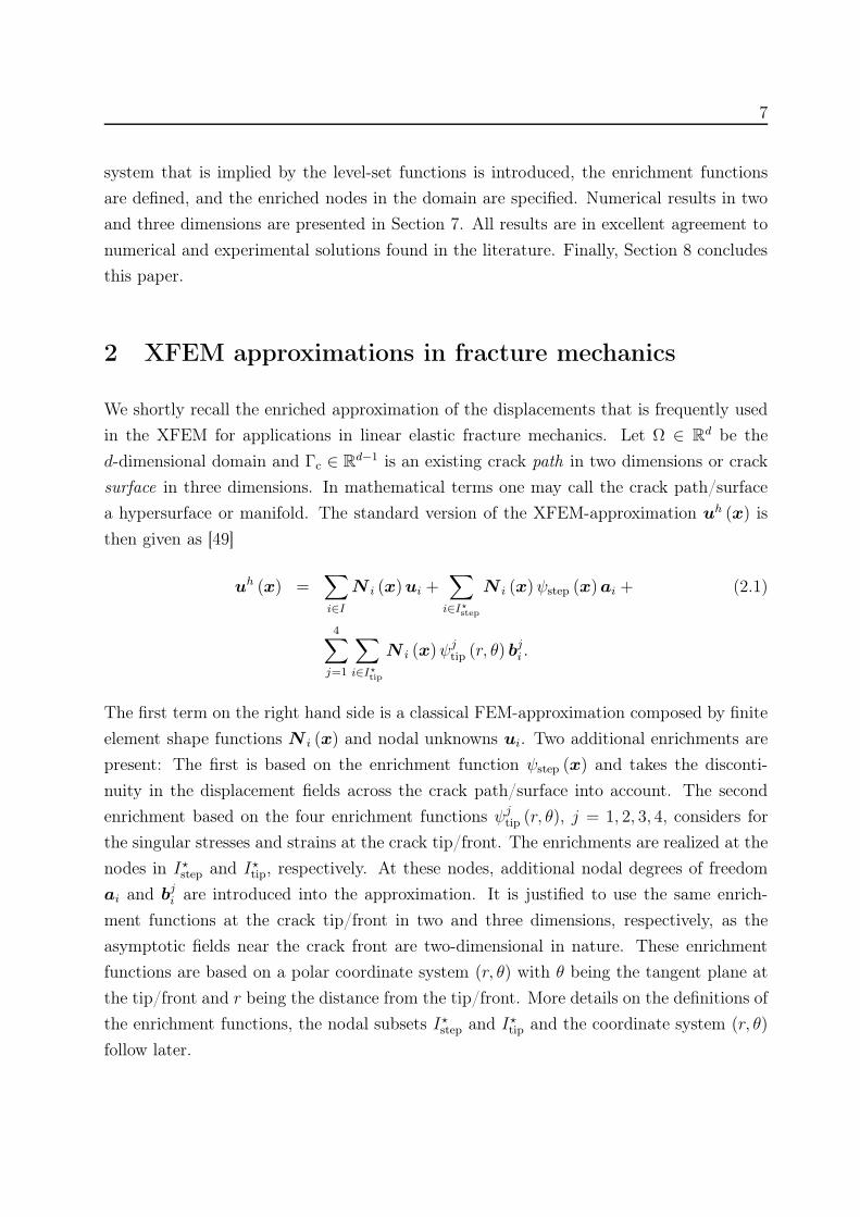
The crack path in two dimensions is discretized by a polygon with nsegm segments, see

Figure 1. The polygon is defined by a set of nodes P i ∈ R2, with i ∈ 1, . . . , nnodes, that

are related by a connectivity matrix C of dimensions nsegm × 2. Each component Cij of C

refers to one of the nodes and hence, 1 ≤ Cij ≤ nnodes.

3.1 Explicit description of cracks in two dimensions 9

Figure 1: A crack path in 2d is described by a polygon. The figure also shows the nodes,the crack tips, and the normal vectors of the segments.

3.1.2 Normal vectors on the crack path

It is useful to associate a normal vector n⋆k to each segment k ∈ 1, . . . , nsegm of the

polygon. Assume that segment k is between the nodes P A = [xA, yA] and P B = [xB, yB],

then

n⋆k =

[

n⋆k,x

n⋆k,y

]

=

[

−(yB − yA)

xB − xA

]

/l, (3.1)

where l =√

(xB − xA)2 + (yB − yA)2 is the length of the segment.

It is noted that the direction of the normal vector is implied by the order of the nodes in

the connectivity matrix. We have assumed here that P A refers to the node in the first

column of C and PB to the second.

3.1.3 Definition of the crack tip(s)

The polygon that describes the crack path is open, hence, it is bounded by two tips. All

inner nodes share two segments and only the two tip nodes are associated with one segment

each. With this criterion, it is simple to automatically extract the tip nodes. However, in

many applications, the crack path is not completely immersed in the domain. For example,

edge cracks in two dimensions have only one crack tip although the corresponding polygon

has two tips. Clearly, all tip nodes that are outside the domain or on the domain boundary

are no (active) crack tips.


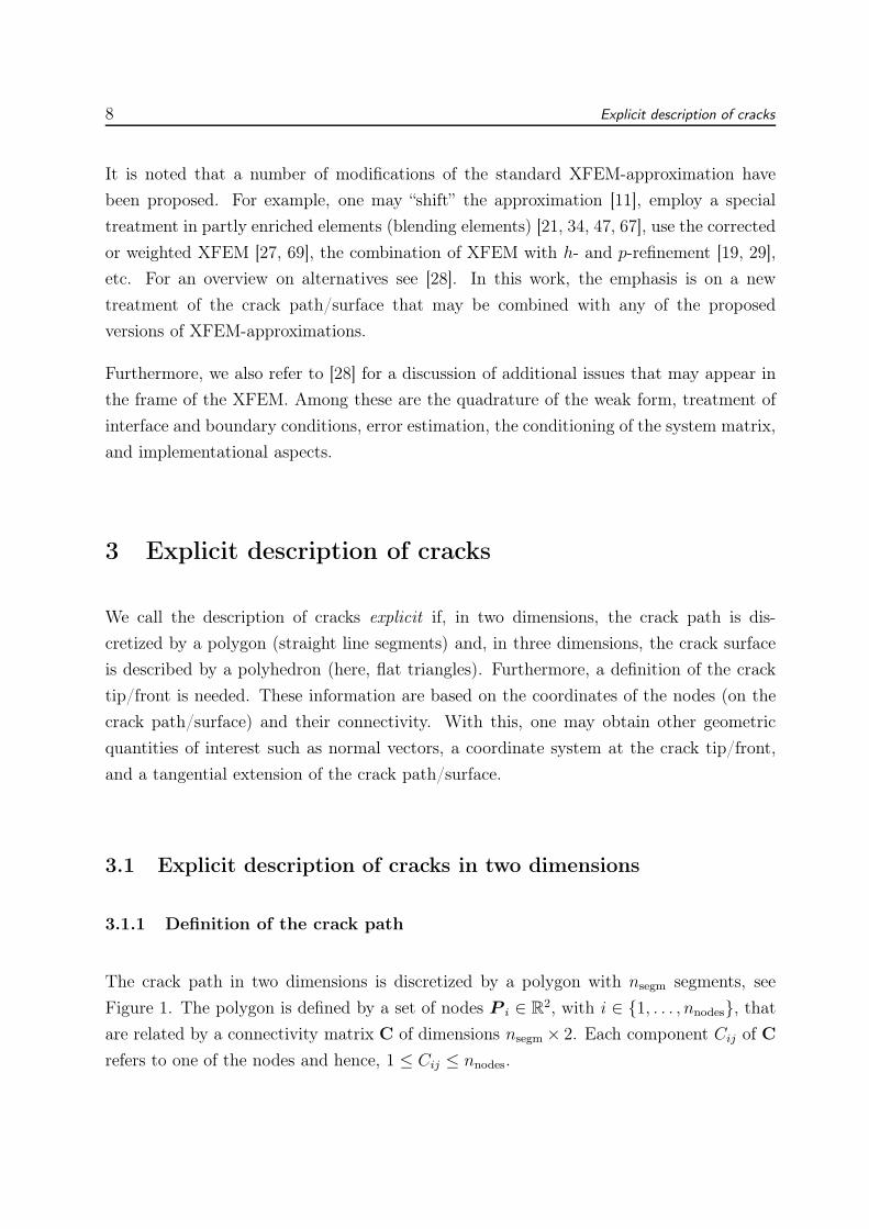
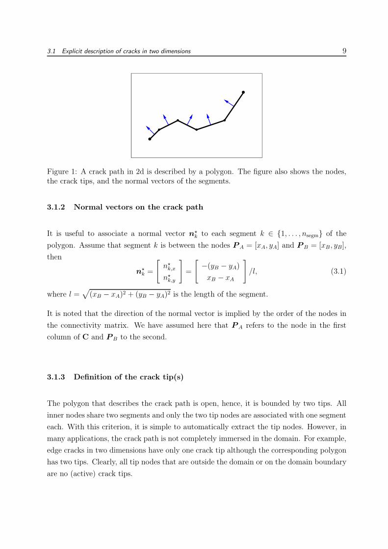
3.1.4 Coordinate system at the crack tip(s)

As discussed in section 3.1.2, normal vectors are easily computed for each of the segments

of the polygon that describes the crack. We are now interested in a coordinate system right

at the tip nodes spanned by the normal and tangential vector, n and t (we omit an index

for the corresponding tip node for brevity). Because the tip nodes belong to one segment

only, one may simply use the normal vector of that segment, n = n⋆k with k being the first

or last segment of the polygon. The tangent vector is easily extracted from the direction of

the first and last segments, respectively, and points outside of the crack path. See Figure

2(a) for a visualization.

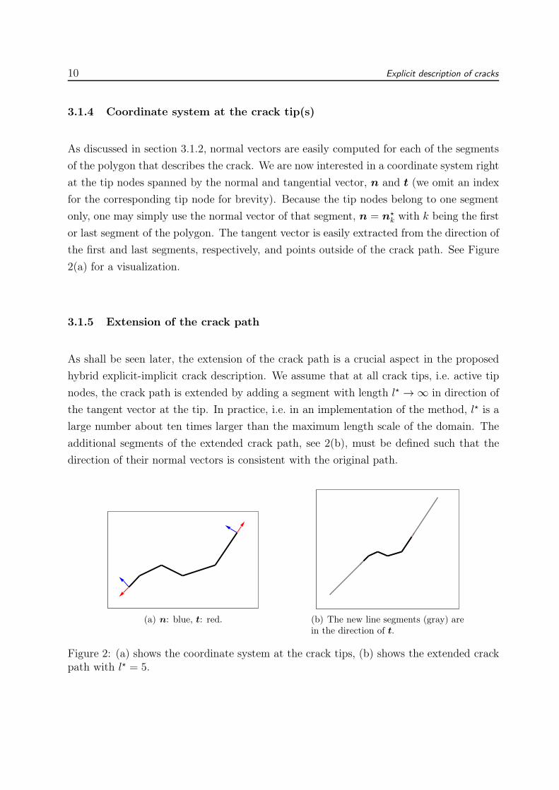
3.1.5 Extension of the crack path

As shall be seen later, the extension of the crack path is a crucial aspect in the proposed

hybrid explicit-implicit crack description. We assume that at all crack tips, i.e. active tip

nodes, the crack path is extended by adding a segment with length l⋆ → ∞ in direction of

the tangent vector at the tip. In practice, i.e. in an implementation of the method, l⋆ is a

large number about ten times larger than the maximum length scale of the domain. The

additional segments of the extended crack path, see 2(b), must be defined such that the

direction of their normal vectors is consistent with the original path.

(a) n: blue, t: red. (b) The new line segments (gray) arein the direction of t.

Figure 2: (a) shows the coordinate system at the crack tips, (b) shows the extended crackpath with l⋆ = 5.

3.2 Explicit description of cracks in three dimensions 11

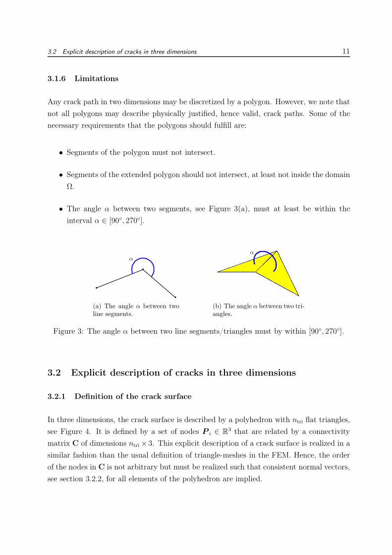
3.1.6 Limitations

Any crack path in two dimensions may be discretized by a polygon. However, we note that

not all polygons may describe physically justified, hence valid, crack paths. Some of the

necessary requirements that the polygons should fulfill are:

• Segments of the polygon must not intersect.

• Segments of the extended polygon should not intersect, at least not inside the domain

Ω.

• The angle α between two segments, see Figure 3(a), must at least be within the

interval α ∈ [90, 270].

(a) The angle α between twoline segments.

(b) The angle α between two tri-angles.

Figure 3: The angle α between two line segments/triangles must by within [90, 270].

3.2 Explicit description of cracks in three dimensions

3.2.1 Definition of the crack surface

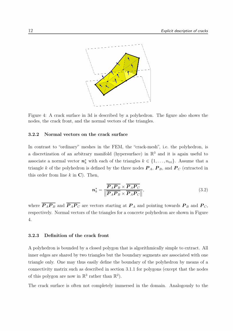
In three dimensions, the crack surface is described by a polyhedron with ntri flat triangles,

see Figure 4. It is defined by a set of nodes P i ∈ R3 that are related by a connectivity

matrix C of dimensions ntri × 3. This explicit description of a crack surface is realized in a

similar fashion than the usual definition of triangle-meshes in the FEM. Hence, the order

of the nodes in C is not arbitrary but must be realized such that consistent normal vectors,

see section 3.2.2, for all elements of the polyhedron are implied.


Figure 4: A crack surface in 3d is described by a polyhedron. The figure also shows thenodes, the crack front, and the normal vectors of the triangles.

3.2.2 Normal vectors on the crack surface

In contrast to “ordinary” meshes in the FEM, the “crack-mesh”, i.e. the polyhedron, is

a discretization of an arbitrary manifold (hypersurface) in R3 and it is again useful to

associate a normal vector n⋆k with each of the triangles k ∈ 1, . . . , ntri. Assume that a

triangle k of the polyhedron is defined by the three nodes P A, P B, and P C (extracted in

this order from line k in C). Then,

n⋆k =

P AP B × P AP C∥

∥P AP B × P AP C

∥

∥

, (3.2)

where P AP B and P AP C are vectors starting at P A and pointing towards P B and P C ,

respectively. Normal vectors of the triangles for a concrete polyhedron are shown in Figure

4.

3.2.3 Definition of the crack front

A polyhedron is bounded by a closed polygon that is algorithmically simple to extract. All

inner edges are shared by two triangles but the boundary segments are associated with one

triangle only. One may thus easily define the boundary of the polyhedron by means of a

connectivity matrix such as described in section 3.1.1 for polygons (except that the nodes

of this polygon are now in R3 rather than R

2).

The crack surface is often not completely immersed in the domain. Analogously to the

3.2 Explicit description of cracks in three dimensions 13

two-dimensional situation, it is a necessary ingredient of the crack description to define

which part of the polygon actually represents the active crack front. For this purpose, one

must carefully restrict the automatically constructed boundary, i.e. the polygon, to the

computational domain.

3.2.4 Coordinate system at the crack front

As discussed above, normal vectors are easily computed for each of the elements of the

polyhedron that describes the crack. On the other hand, right at the nodes and along

the edges, the normal vectors are discontinuous. The situation is similar to discontinuous

stress and strain fields resulting from C0-continuous approximations of the displacement

fields. However, one may still obtain smooth fields by averaging.

Let us assume we are interested in the normal vector of node m on the crack front. This

node is shared by nt triangles, each with a normal vector n⋆k and an area Ak. Then an

averaged normal vector at node m is given by

nm =n′

m

‖n′m‖

with n′m =

∑nt

i=1Ai · n⋆i

∑nt

i=1Ai

. (3.3)

This normal vector could, in fact, be evaluated at all nodes of the polyhedron. However,

it is only needed at the nodes on the crack front. The next step is the computation of a

tangent vector to the front and a similar averaging is employed. Assume that node m is

shared by ns front segments (ns is either 1 or 2), and the direction of each segment k is

given by q⋆k, ‖q⋆

k‖ = 1, and its length by lk. Then, the tangent vector at the front node m

is computed as

qm =q′m

‖q′m‖

with q′m =

∑ns

i=1 li · q⋆i

∑ns

i=1 li. (3.4)

We note that nm and qm are not necessarily orthogonal but at least linearly independent.

As such, we are now ready to define a vector tm for each node m on the crack front which

can be interpreted as a tangential extension of the crack surface that is normal to the crack

front,

tm = qm × nm. (3.5)

Mathematically, it is in general not possible to find a vector tm that is within the plane of

all triangles that share node m. The resulting coordinate systems at the front nodes are

shown in Figure 5(a).


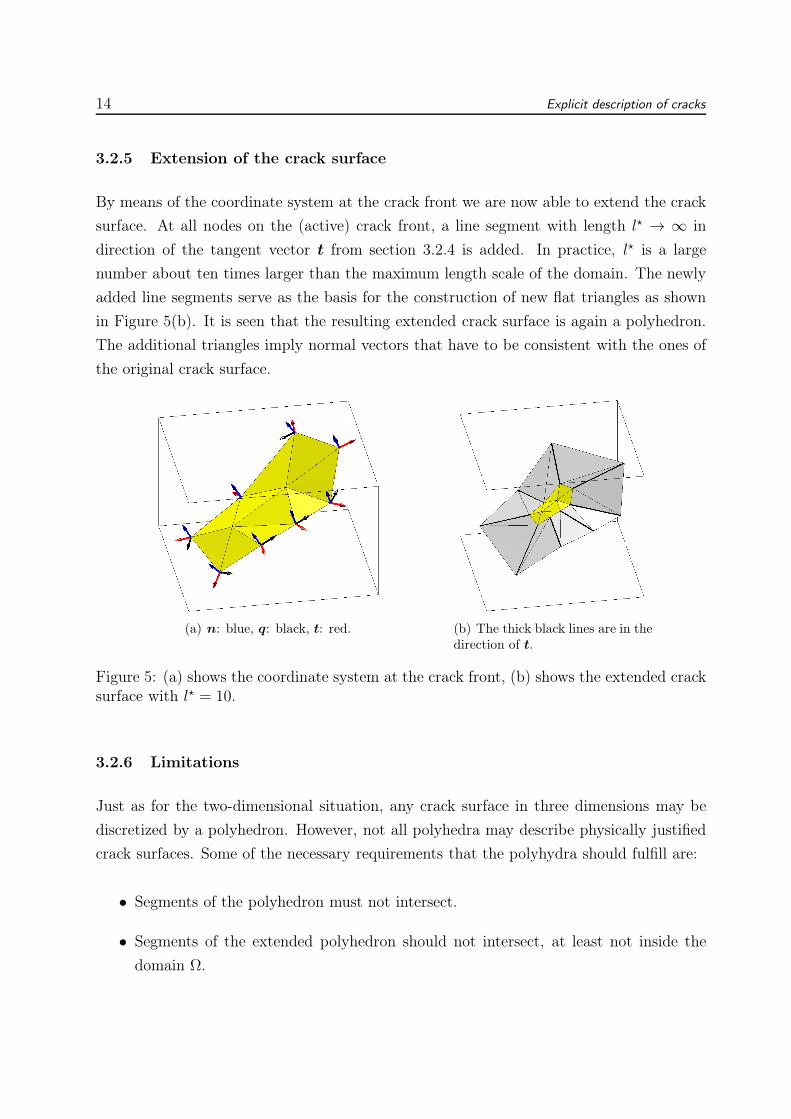
3.2.5 Extension of the crack surface

By means of the coordinate system at the crack front we are now able to extend the crack

surface. At all nodes on the (active) crack front, a line segment with length l⋆ → ∞ in

direction of the tangent vector t from section 3.2.4 is added. In practice, l⋆ is a large

number about ten times larger than the maximum length scale of the domain. The newly

added line segments serve as the basis for the construction of new flat triangles as shown

in Figure 5(b). It is seen that the resulting extended crack surface is again a polyhedron.

The additional triangles imply normal vectors that have to be consistent with the ones of

the original crack surface.

(a) n: blue, q: black, t: red. (b) The thick black lines are in thedirection of t.

Figure 5: (a) shows the coordinate system at the crack front, (b) shows the extended cracksurface with l⋆ = 10.

3.2.6 Limitations

Just as for the two-dimensional situation, any crack surface in three dimensions may be

discretized by a polyhedron. However, not all polyhedra may describe physically justified

crack surfaces. Some of the necessary requirements that the polyhydra should fulfill are:

• Segments of the polyhedron must not intersect.

• Segments of the extended polyhedron should not intersect, at least not inside the

domain Ω.

15

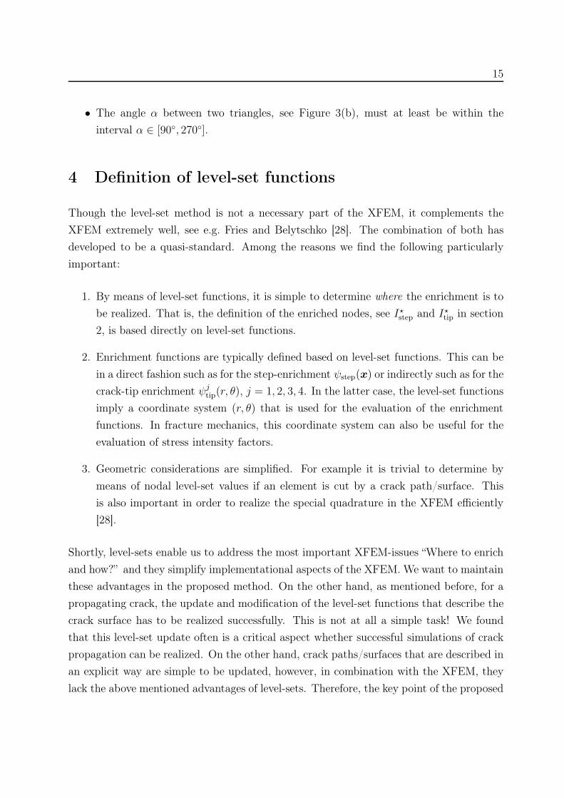
• The angle α between two triangles, see Figure 3(b), must at least be within the

interval α ∈ [90, 270].

4 Definition of level-set functions

Though the level-set method is not a necessary part of the XFEM, it complements the

XFEM extremely well, see e.g. Fries and Belytschko [28]. The combination of both has

developed to be a quasi-standard. Among the reasons we find the following particularly

important:

1. By means of level-set functions, it is simple to determine where the enrichment is to

be realized. That is, the definition of the enriched nodes, see I⋆step and I⋆tip in section

2, is based directly on level-set functions.

2. Enrichment functions are typically defined based on level-set functions. This can be

in a direct fashion such as for the step-enrichment ψstep(x) or indirectly such as for the

crack-tip enrichment ψjtip(r, θ), j = 1, 2, 3, 4. In the latter case, the level-set functions

imply a coordinate system (r, θ) that is used for the evaluation of the enrichment

functions. In fracture mechanics, this coordinate system can also be useful for the

evaluation of stress intensity factors.

3. Geometric considerations are simplified. For example it is trivial to determine by

means of nodal level-set values if an element is cut by a crack path/surface. This

is also important in order to realize the special quadrature in the XFEM efficiently

[28].

Shortly, level-sets enable us to address the most important XFEM-issues “Where to enrich

and how?” and they simplify implementational aspects of the XFEM. We want to maintain

these advantages in the proposed method. On the other hand, as mentioned before, for a

propagating crack, the update and modification of the level-set functions that describe the

crack surface has to be realized successfully. This is not at all a simple task! We found

that this level-set update often is a critical aspect whether successful simulations of crack

propagation can be realized. On the other hand, crack paths/surfaces that are described in

an explicit way are simple to be updated, however, in combination with the XFEM, they

lack the above mentioned advantages of level-sets. Therefore, the key point of the proposed


method is the combination of explicit crack descriptions with the implicit description by

level-sets.

In contrast to the standard treatment of cracks with level-sets as proposed by Stolarska in

[63] or the treatment based on vector level-sets as discussed in Ventura et al. [70, 68], we

suggest the use of three level-set functions. The advantage is that these level-set functions

extend from two to three dimensions in a straightforward manner and are readily computed

for a given, explicit crack description. We note that this is not the case for the standard

description by two (orthogonal) level-set functions as proposed in [63].

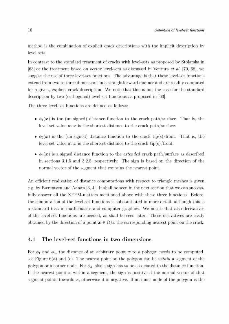
The three level-set functions are defined as follows:

• φ1(x) is the (un-signed) distance function to the crack path/surface. That is, the

level-set value at x is the shortest distance to the crack path/surface.

• φ2(x) is the (un-signed) distance function to the crack tip(s)/front. That is, the

level-set value at x is the shortest distance to the crack tip(s)/front.

• φ3(x) is a signed distance function to the extended crack path/surface as described

in sections 3.1.5 and 3.2.5, respectively. The sign is based on the direction of the

normal vector of the segment that contains the nearest point.

An efficient realization of distance computations with respect to triangle meshes is given

e.g. by Bærentzen and Aanæs [3, 4]. It shall be seen in the next section that we can success-

fully answer all the XFEM-matters mentioned above with these three functions. Before,

the computation of the level-set functions is substantiated in more detail, although this is

a standard task in mathematics and computer graphics. We notice that also derivatives

of the level-set functions are needed, as shall be seen later. These derivatives are easily

obtained by the direction of a point x ∈ Ω to the corresponding nearest point on the crack.

4.1 The level-set functions in two dimensions

For φ1 and φ3, the distance of an arbitrary point x to a polygon needs to be computed,

see Figure 6(a) and (c). The nearest point on the polygon can be within a segment of the

polygon or a corner node. For φ3, also a sign has to be associated to the distance function.

If the nearest point is within a segment, the sign is positive if the normal vector of that

segment points towards x, otherwise it is negative. If an inner node of the polygon is the

4.2 The level-set functions in three dimensions 17

nearest point, then two segments share this node. The normal vectors of both segments

must either point towards x or not, leading to a positive or negative sign, respectively.

No sign could be determined if one of the two normal vectors points towards x and the

other not. This can only be the case if the angle α between two segments is not within

[90, 270], see section 3.1.6. For a crack path, such a situation is unphysical; hence, this

does not pose a restriction of the proposed method.

For the computation of φ2, the distance of an arbitrary point x to the crack tip(s) needs

to be computed. Such a computation is particularly simple. A graphical representation of

φ2 is seen in Figure 6(b).

(a) φ1(x) (b) φ2(x)

(c) φ3(x)

Figure 6: The three level-set functions in two dimensions.

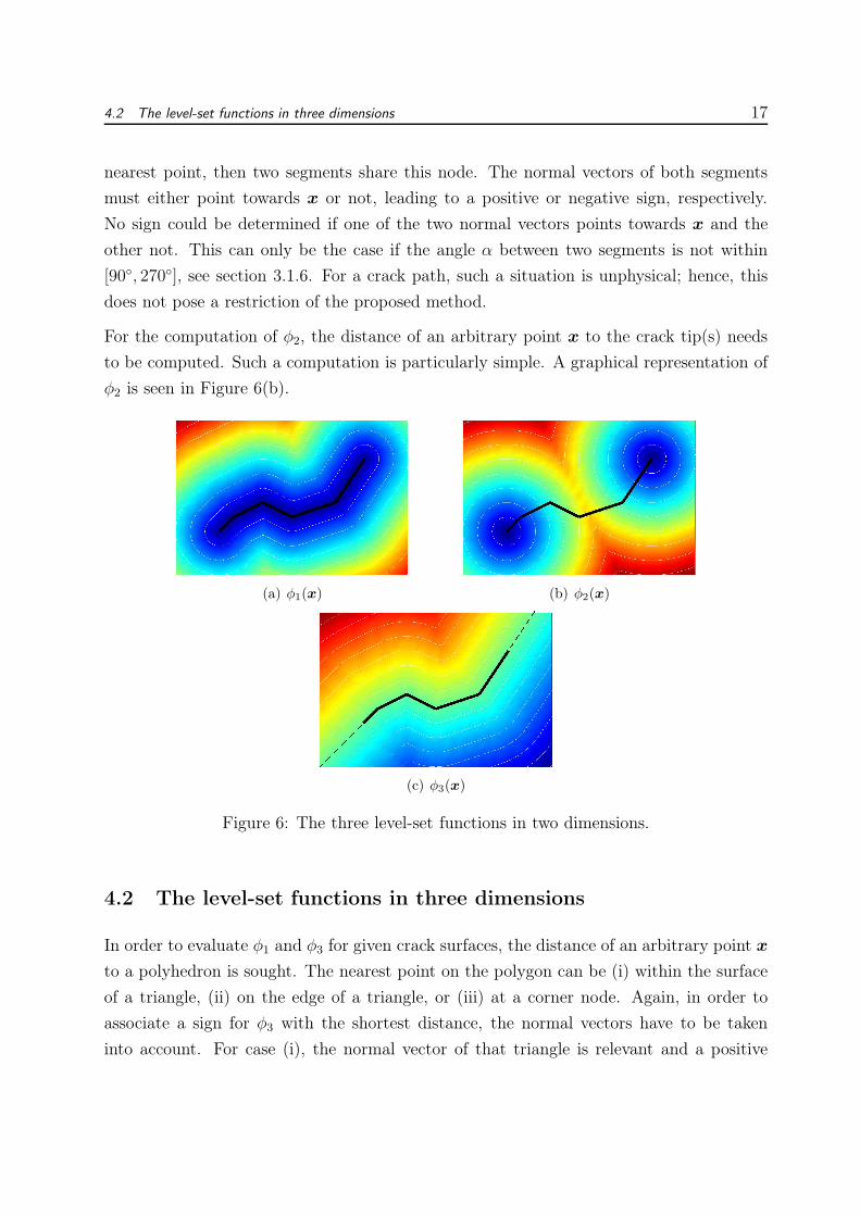
4.2 The level-set functions in three dimensions

In order to evaluate φ1 and φ3 for given crack surfaces, the distance of an arbitrary point x

to a polyhedron is sought. The nearest point on the polygon can be (i) within the surface

of a triangle, (ii) on the edge of a triangle, or (iii) at a corner node. Again, in order to

associate a sign for φ3 with the shortest distance, the normal vectors have to be taken

into account. For case (i), the normal vector of that triangle is relevant and a positive


sign results if this vector points towards x. For case (ii), the edge is possibly shared by

two triangles and the direction of their normal vectors must coincide at x. In case of (iii),

the normal vectors of all triangles that share the nearest node must coincide at x. These

requirements again impose certain conditions on the angles between the triangles; however,

this does not pose a restriction of the method for crack applications. A visualization of the

level-sets φ1 and φ3 by means of isosurfaces is given in Figures 7 and 9. These isosurfaces

refer to the polyhedron shown in Figure 4.

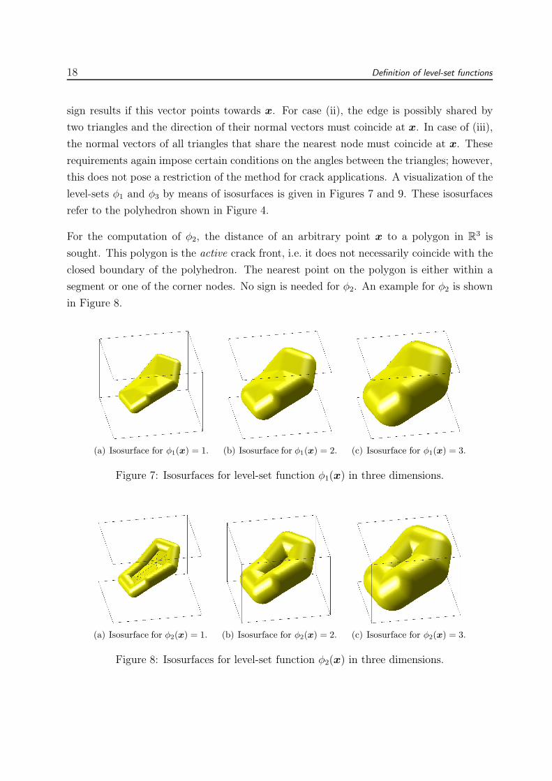
For the computation of φ2, the distance of an arbitrary point x to a polygon in R3 is

sought. This polygon is the active crack front, i.e. it does not necessarily coincide with the

closed boundary of the polyhedron. The nearest point on the polygon is either within a

segment or one of the corner nodes. No sign is needed for φ2. An example for φ2 is shown

in Figure 8.

(a) Isosurface for φ1(x) = 1. (b) Isosurface for φ1(x) = 2. (c) Isosurface for φ1(x) = 3.

Figure 7: Isosurfaces for level-set function φ1(x) in three dimensions.

(a) Isosurface for φ2(x) = 1. (b) Isosurface for φ2(x) = 2. (c) Isosurface for φ2(x) = 3.


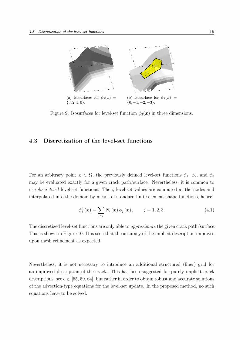
4.3 Discretization of the level-set functions 19

(a) Isosurfaces for φ3(x) =3, 2, 1, 0.

(b) Isosurface for φ3(x) =0,−1,−2,−3.


4.3 Discretization of the level-set functions

For an arbitrary point x ∈ Ω, the previously defined level-set functions φ1, φ2, and φ3

may be evaluated exactly for a given crack path/surface. Nevertheless, it is common to

use discretized level-set functions. Then, level-set values are computed at the nodes and

interpolated into the domain by means of standard finite element shape functions, hence,

φhj (x) =

∑

i∈I

Ni (x)φj (x) , j = 1, 2, 3. (4.1)

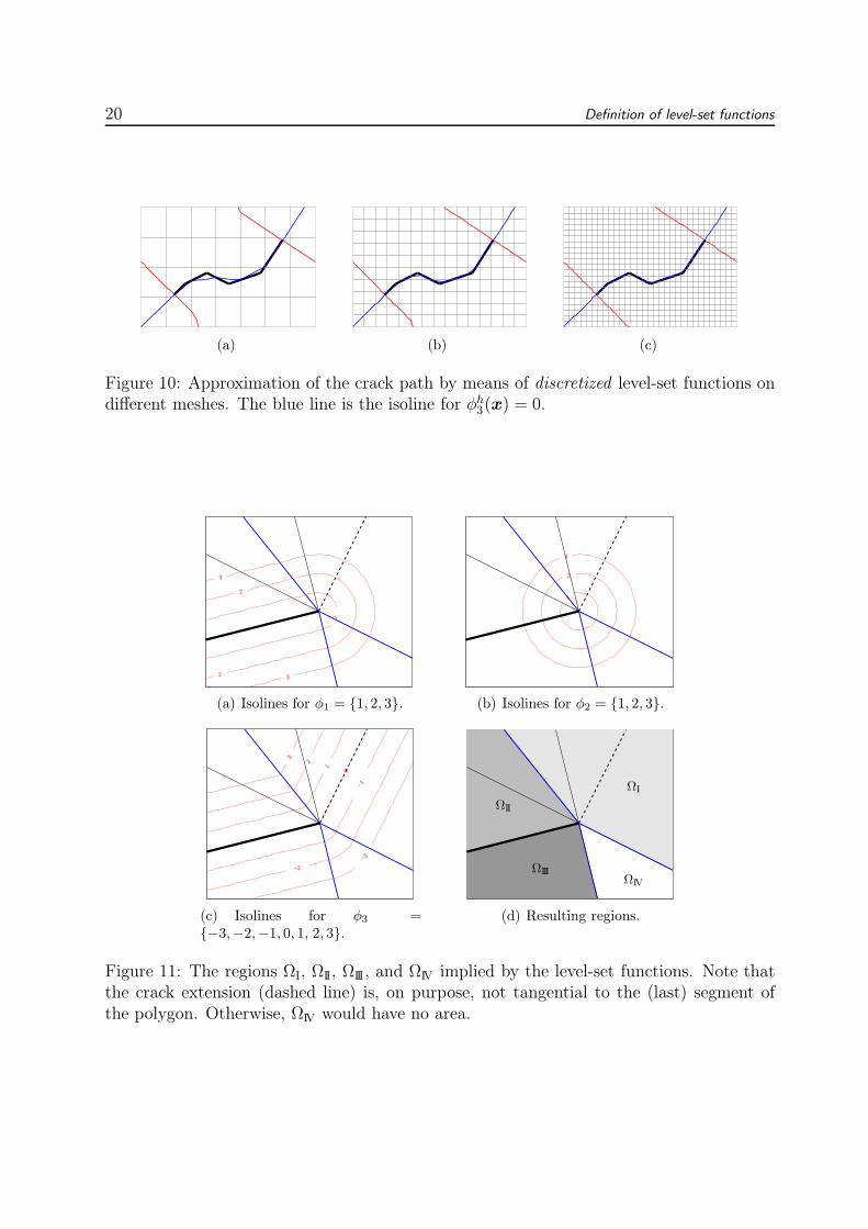
The discretized level-set functions are only able to approximate the given crack path/surface.

This is shown in Figure 10. It is seen that the accuracy of the implicit description improves

upon mesh refinement as expected.

Nevertheless, it is not necessary to introduce an additional structured (finer) grid for

an improved description of the crack. This has been suggested for purely implicit crack

descriptions, see e.g. [55, 59, 64], but rather in order to obtain robust and accurate solutions

of the advection-type equations for the level-set update. In the proposed method, no such

equations have to be solved.


(a) (b) (c)

Figure 10: Approximation of the crack path by means of discretized level-set functions ondifferent meshes. The blue line is the isoline for φh

3(x) = 0.

1

2

2 3

3

(a) Isolines for φ1 = 1, 2, 3.

1

2

3

(b) Isolines for φ2 = 1, 2, 3.

−3

−2

−1

0

1

2

3

(c) Isolines for φ3 =−3,−2,−1, 0, 1, 2, 3.

(d) Resulting regions.

Figure 11: The regions ΩI, ΩII, ΩIII, and ΩIV implied by the level-set functions. Note thatthe crack extension (dashed line) is, on purpose, not tangential to the (last) segment ofthe polygon. Otherwise, ΩIV would have no area.

21

5 Coordinate systems implied by the level-set functions

5.1 The coordinate system (r, θ)

Let us now define a coordinate system (r, θ) based on the three level-set functions defined

above. The definition of r is straightforward

r (x) = φ2 (x) . (5.1)

For the definition of θ it is useful to define

θ⋆ (x) = sin−1 φ3 (x)

φ2 (x), (5.2)

and to decompose the domain into several regions

ΩI = x : φ1 6= |φ3| , (5.3)

ΩII = x : φ1 = |φ3| , φ2 6= |φ3| , φ3 > 0 , (5.4)

ΩIII = x : φ1 = |φ3| , φ2 6= |φ3| , φ3 ≤ 0 , (5.5)

ΩIV = x : φ1 = |φ3| , φ2 = |φ3| . (5.6)

Then, we define θ as

θ (x) =

θ⋆ (x) ∀x ∈ ΩI,

π − θ⋆ (x) ∀x ∈ ΩII,

−π − θ⋆ (x) ∀x ∈ ΩIII,

θ⋆ (x) = ±π2

∀x ∈ ΩIV.

(5.7)

The regions ΩI, ΩII, ΩIII, and ΩIV are shown in Figure 11. It is important to note that, in

this figure, the extension of the polygon is, on purpose, not in the direction of the tangent

vector at the tip node. The reason is that in three dimensions, the tangent vector is in

general anyway not tangential to all neighboring triangles, as discussed in Section 3.2.4.

This would only be the case for planar crack surfaces, but the situation considered here is

more general. Only in two dimensions, one can ensure a “perfect” extension of the crack

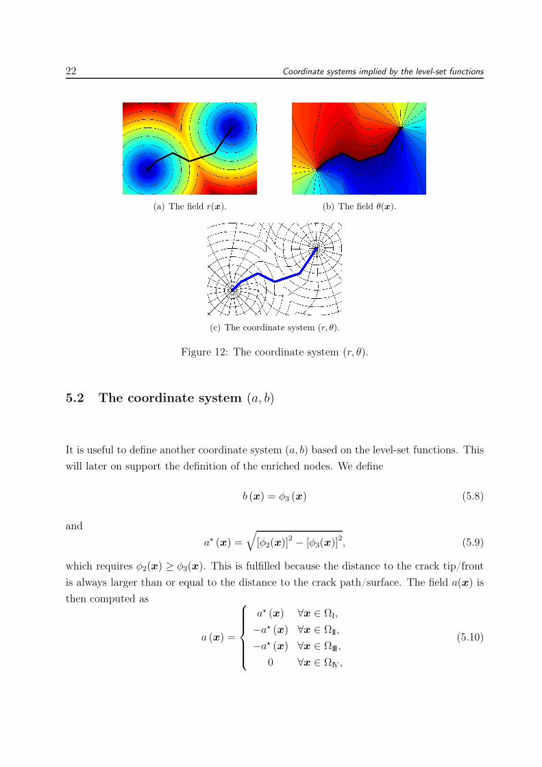
path. In the region ΩIV, the angle θ = ±π/2. Visualizations of r (x), θ (x) and the resulting

coordinate system are shown in Figure 12(a) to (c).


(a) The field r(x). (b) The field θ(x).

(c) The coordinate system (r, θ).

Figure 12: The coordinate system (r, θ).

5.2 The coordinate system (a, b)

It is useful to define another coordinate system (a, b) based on the level-set functions. This

will later on support the definition of the enriched nodes. We define

b (x) = φ3 (x) (5.8)

and

a⋆ (x) =

√

[φ2(x)]2 − [φ3(x)]

2, (5.9)

which requires φ2(x) ≥ φ3(x). This is fulfilled because the distance to the crack tip/front

is always larger than or equal to the distance to the crack path/surface. The field a(x) is

then computed as

a (x) =

a⋆ (x) ∀x ∈ ΩI,

−a⋆ (x) ∀x ∈ ΩII,

−a⋆ (x) ∀x ∈ ΩIII,

0 ∀x ∈ ΩIV,

(5.10)

5.3 The set of enriched nodes 23

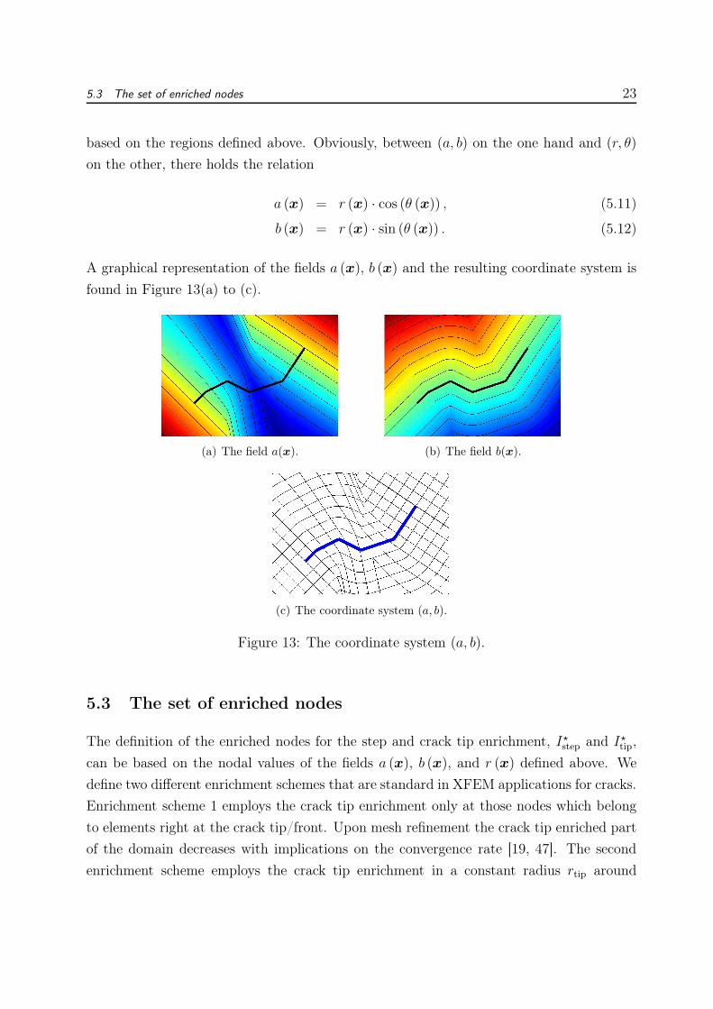
based on the regions defined above. Obviously, between (a, b) on the one hand and (r, θ)

on the other, there holds the relation

a (x) = r (x) · cos (θ (x)) , (5.11)

b (x) = r (x) · sin (θ (x)) . (5.12)

A graphical representation of the fields a (x), b (x) and the resulting coordinate system is

found in Figure 13(a) to (c).

(a) The field a(x). (b) The field b(x).

(c) The coordinate system (a, b).

Figure 13: The coordinate system (a, b).

5.3 The set of enriched nodes

The definition of the enriched nodes for the step and crack tip enrichment, I⋆step and I⋆tip,

can be based on the nodal values of the fields a (x), b (x), and r (x) defined above. We

define two different enrichment schemes that are standard in XFEM applications for cracks.

Enrichment scheme 1 employs the crack tip enrichment only at those nodes which belong

to elements right at the crack tip/front. Upon mesh refinement the crack tip enriched part

of the domain decreases with implications on the convergence rate [19, 47]. The second

enrichment scheme employs the crack tip enrichment in a constant radius rtip around


the crack tip/front. This part of the domain remains constant upon mesh refinement,

however, with negative implications on the conditioning of the system matrix [47]. In both

enrichment schemes, all nodes that belong to elements cut by the crack path/surface and

do not belong to the crack tip enriched nodes are enriched with the step enrichment.

Formally, we start the definition of I⋆step and I⋆tip, by introducing element sets. The domain

Ω is discretized by nel (two or three-dimensional) elements. Let Ielk be the element nodes

of element k. We define

N 1tip =

k ∈

1, . . . , nel

: mini∈Iel

k

(a (xi)) ·maxi∈Iel

k

(a (xi)) < 0 and (5.13)

mini∈Iel

k

(b (xi)) ·maxi∈Iel

k

(b (xi)) < 0

N 2tip =

k ∈

1, . . . , nel

: mini∈Iel

k

(r (xi)) ≤ rtip

⋃

N 1tip (5.14)

In Equation (5.14), the union with N 1tip on the right hand side ensures that N 2

tip is also not

empty for extremely small rtip. Furthermore,

N jstep =

k ∈

1, . . . , nel

: maxi∈Iel

k

(a (xi)) < 0 and (5.15)

mini∈Iel

k

(b (xi)) ·maxi∈Iel

k

(b (xi)) < 0

\ N jtip, j = 1, 2. (5.16)

This definition ensures that no elements in N jstep appear also in N j

tip.

We note that in cases where some of the requirements on the explicit description of the crack

are not met, see Section 3, it can be useful to ensure the validity of the sets defined above.

Then, accurate results can be obtained even if not all requirements are met; an example

is the test case presented in Section 7.1.5. The additional check is based on the maximum

element length h of each element; we define hk as the maximum element diagonal of element

k. Then, from N 1tip, one should exclude all elements for which maxi∈Iel

k(r (xi)) > hk, and

from N jstep all elements for which maxi∈Iel

k(φ1 (xi)) > hk.

The set of enriched nodes I⋆tip follows as the union of all elements nodes in N jtip, with

5.4 The enrichment functions 25

j = 1, 2 depending on the chosen enrichment scheme, hence

I⋆tip =⋃

k∈Njtip

Ielk , with j = 1 or 2. (5.17)

The set of step-enriched nodes I⋆step is then defined as

I⋆step =

⋃

k∈Njstep

Ielk

\ I⋆tip, with j = 1 or 2. (5.18)

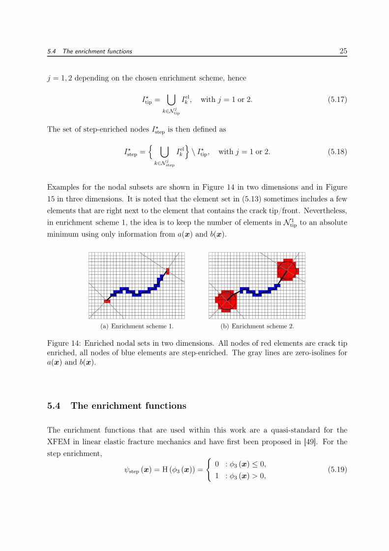
Examples for the nodal subsets are shown in Figure 14 in two dimensions and in Figure

15 in three dimensions. It is noted that the element set in (5.13) sometimes includes a few

elements that are right next to the element that contains the crack tip/front. Nevertheless,

in enrichment scheme 1, the idea is to keep the number of elements in N 1tip to an absolute

minimum using only information from a(x) and b(x).

(a) Enrichment scheme 1. (b) Enrichment scheme 2.

Figure 14: Enriched nodal sets in two dimensions. All nodes of red elements are crack tipenriched, all nodes of blue elements are step-enriched. The gray lines are zero-isolines fora(x) and b(x).

5.4 The enrichment functions

The enrichment functions that are used within this work are a quasi-standard for the

XFEM in linear elastic fracture mechanics and have first been proposed in [49]. For the

step enrichment,

ψstep (x) = H (φ3 (x)) =

0 : φ3 (x) ≤ 0,

1 : φ3 (x) > 0,(5.19)


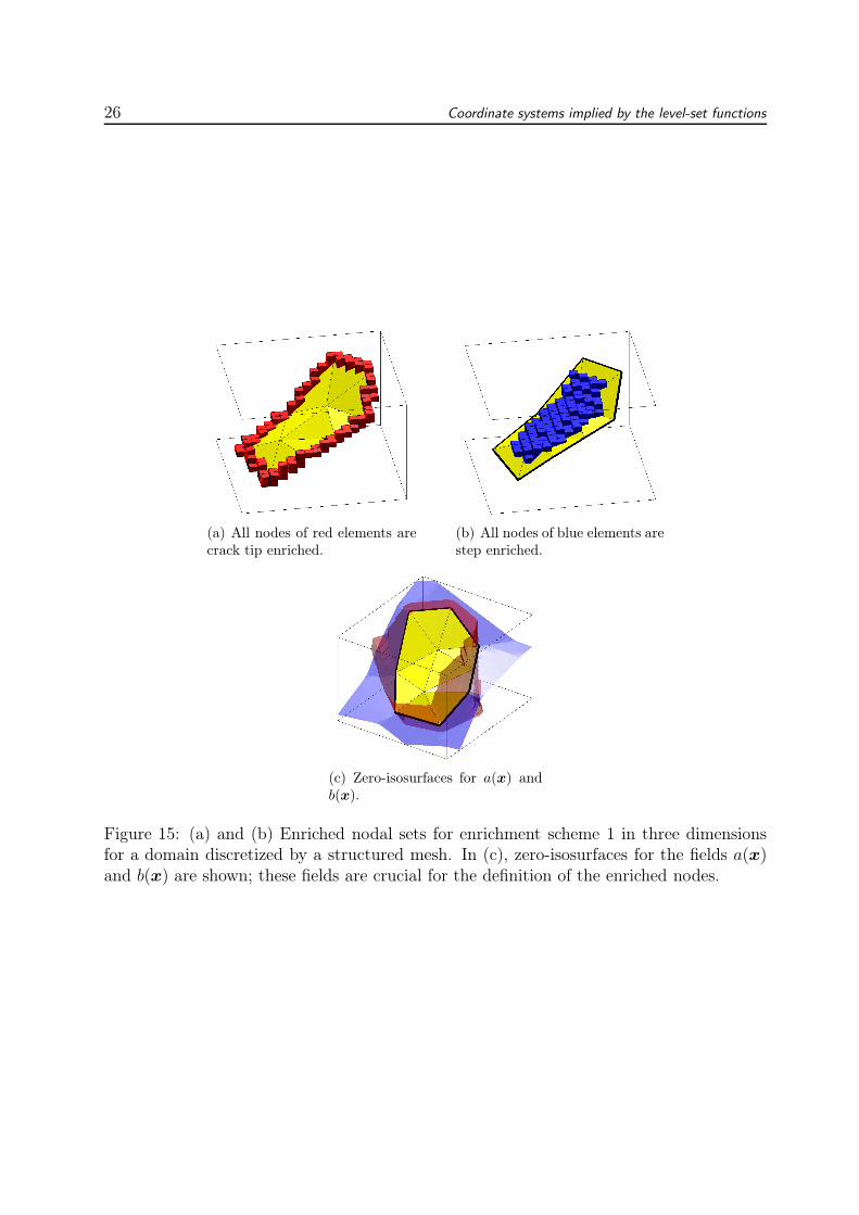
(a) All nodes of red elements arecrack tip enriched.

(b) All nodes of blue elements arestep enriched.

(c) Zero-isosurfaces for a(x) andb(x).

Figure 15: (a) and (b) Enriched nodal sets for enrichment scheme 1 in three dimensionsfor a domain discretized by a structured mesh. In (c), zero-isosurfaces for the fields a(x)and b(x) are shown; these fields are crucial for the definition of the enriched nodes.

27

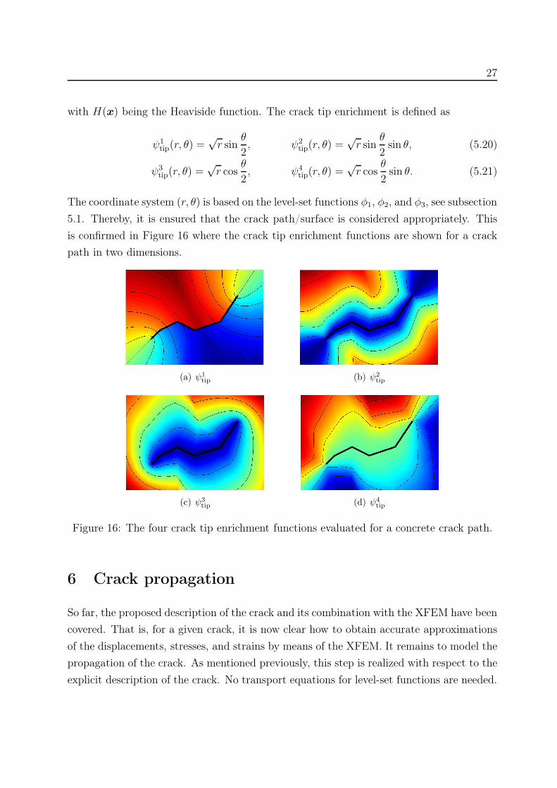
with H(x) being the Heaviside function. The crack tip enrichment is defined as

ψ1tip(r, θ) =

√r sin

θ

2, ψ2

tip(r, θ) =√r sin

θ

2sin θ, (5.20)

ψ3tip(r, θ) =

√r cos

θ

2, ψ4

tip(r, θ) =√r cos

θ

2sin θ. (5.21)

The coordinate system (r, θ) is based on the level-set functions φ1, φ2, and φ3, see subsection

5.1. Thereby, it is ensured that the crack path/surface is considered appropriately. This

is confirmed in Figure 16 where the crack tip enrichment functions are shown for a crack

path in two dimensions.

(a) ψ1tip (b) ψ2

tip

(c) ψ3tip (d) ψ4

tip

Figure 16: The four crack tip enrichment functions evaluated for a concrete crack path.

6 Crack propagation

So far, the proposed description of the crack and its combination with the XFEM have been

covered. That is, for a given crack, it is now clear how to obtain accurate approximations

of the displacements, stresses, and strains by means of the XFEM. It remains to model the

propagation of the crack. As mentioned previously, this step is realized with respect to the

explicit description of the crack. No transport equations for level-set functions are needed.

28 Crack propagation

Each crack increment is defined by the motion of the crack front. It is natural to define

where to go and how far for each of the nodes on the crack front. Other discrete positions on

the crack front (such as the center of each line segment on the front) could be chosen as well

but, in this work, we move the front nodes. The movement may be modeled by a number

of different approaches and we do not see a major contribution of this paper in this aspect.

One could, for example, base the crack propagation on stress intensity factors [43, 72],

the J-integral [20, 61], configurational forces [26, 38] etc. We note that stress intensity

factors are frequently used in two dimensions, however, they sometimes pose difficulties

and uncertainties in three dimensions as noted e.g. in [58, 71]. The combination of the

proposed treatment of the crack within the XFEM on the one hand and configurational

forces on the other hand was particularly successful and will be reported in a forthcoming

publication. In this work, however, we reduce ourselves to a very simple yet effective

approach for the modeling of the propagation.

6.1 The crack increment

Based on Erdogan and Sih [25], the approach presented here assumes that the crack grows

in the direction of the maximum circumferential (hoop) stress. For each of the front nodes,

stresses are evaluated at nc discrete points on a circle with radius rc around this node. This

“stress circle” is placed in the plane spanned by n and t at that front node, see Subsection

3.1.4 and 3.2.4. Furthermore, an angle θc is associated with respect to each of the discrete

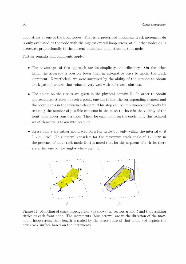
points, with θc = 0 in the direction of t. The situation is shown in Figure 17(a).

As shall be confirmed in the numerical results below, it is useful to relate the radius

rc of the circle with the (maximum) crack increment da. Reasonable choices are often

0.1 · da ≤ rc ≤ da. Clearly, valid ranges for rc are bounded from below by the element size

h at the crack tip/front (it is reasonable to assume that rc should be at least larger than

0.5 · h) and from above by the region where the fields are dominated by the crack modes.

We do not find these bounds to be very restrictive, i.e. it is not difficult to specify suitable

values for the radius.

In order to obtain the hoop stress for each of the nc discrete points on the circle, the stress

tensor σxyz with respect to the Cartesian coordinate system (obtained from the XFEM

approximation) is mapped into the rotated front coordinate system defined by n, t, and

q at that node, leading to σntq. We neglect the components in the direction q tangent to

6.1 The crack increment 29

the crack front in order to obtain σnt =

[

σnn σnt

σnt σtt

]

; in two dimensions, this tensor is

immediately obtained as q is not present. This step is justified as long as the influence of

the third crack mode (shearing mode) is negligible.

Finally, the hoop stress at the current point on the circle is given by

σθθ = σnn sin2(θc) + σtt cos

2(θc)− σnt sin(2 · θc). (6.1)

It is simple to find the propagation angle θincr where the hoop stress is maximum. The

direction where the node on the crack front is moving is then uniquely defined by this angle

θincr in the plane spanned by n and t. We call this criterion “max(σθθ)”-criterion.

It is important to note that in C0-continuous approximations, the stress fields are discon-

tinuous over the element boundaries. Consequently, there are possibly awkward jumps in

the stress profiles on the circles. It is thus recommended to first obtain smooth stress fields

in a post-processing step from the XFEM-solution. Then, by means of the nodal values of

these smoothed stress fields, it is a pure interpolation problem to obtain the stress for a

given point x ∈ Ω. That is, one does not have to evaluate the stresses directly via the ex-

tended approximation (2.1) which would be discontinuous over the element boundaries. All

results presented later are obtained by means of smoothed stress fields and interpolation.

This smoothing step justifies the introduction of a second criterion, that has the same

physical motivation than the “max(σθθ)”-criterion. In addition to the hoop stresses σθθ, see

Equation (6.1), we evaluate the shear stress

σrθ = sin(θc) cos(θc) (σnn − σtt) + σnt cos(2 · θc) (6.2)

at each of the points on the stress circles. Then, the angle θincr is computed for which

σrθ = 0. There is possibly more than one angle for which σrθ = 0. Then, all these angles

are extracted and the one with the largest σθθ is chosen. We call this approach “σrθ = 0”-

criterion. For example in the context of models where the direction is based on computed

stress intensity factors, the two criteria coincide. However, in the context of the proposed

model, the two approaches yield similar yet not identical angles. In fact, it shall be seen

that the “σrθ = 0”-criterion is superior when compared to the “max(σθθ)”-criterion.

In three dimensions, once θincr is computed for each of the nodes on the crack front (by one

of the two approaches), the length of each crack increment is scaled by the maximum overall

30 Crack propagation

hoop stress at one of the front nodes. That is, a prescribed maximum crack increment da

is only evaluated at the node with the highest overall hoop stress, at all other nodes da is

decreased proportionally to the current maximum hoop stress at that node.

Further remarks and comments apply:

• The advantages of this approach are its simplicity and efficiency. On the other

hand, the accuracy is possibly lower than in alternative ways to model the crack

increment. Nevertheless, we were surprised by the ability of the method to obtain

crack paths/surfaces that coincide very well with reference solutions.

• The points on the circles are given in the physical domain Ω. In order to obtain

approximated stresses at such a point, one has to find the corresponding element and

the coordinates in the reference element. This step can be implemented efficiently by

reducing the number of possible elements in the mesh to those in the vicinity of the

front node under consideration. Then, for each point on the circle, only this reduced

set of elements is taken into account.

• Stress points are rather not placed on a full circle but only within the interval θc ∈[−75,+75]. This interval considers for the maximum crack angle of ±70.529 in

the presence of only crack mode II. It is noted that for this segment of a circle, there

are either one or two angles where σrθ = 0.

(a) (b)

Figure 17: Modeling of crack propagation: (a) shows the vectors n and t and the resultingcircles at each front node. The increments (blue arrows) are in the direction of the max-imum hoop stress; their length is scaled by the stress state at that node. (b) depicts thenew crack surface based on the increments.

6.2 Update of the crack path/surface 31

6.2 Update of the crack path/surface

Once the movement of each node on the crack front is defined, the crack path/surface needs

to be updated. In two dimensions, this is realized by adding line segments at the crack

tips. In three dimensions, flat triangles are constructed such that the nodal increments

are considered for appropriately, see Figure 17(b). In terms of the implementation, this

step requires the definition of new nodes P i and an update of the connectivity matrix C,

cf. Section 3. Furthermore, the definition of the crack tip(s)/front has to be updated.

In Figure 17(b), the displacement of each front node is shown by a blue arrow whose

length varies depending on the stress state at that node. In order to obtain the new crack

surface, the gray triangles are added to the yellow triangles of the previous crack surface.

The normal vectors of all triangles of the polyhedron must point to the same side of the

surface. Furthermore, the crack front of the previous surface (blue polygon) needs to be

updated (black polygon).

6.3 Update of the extended crack path/surface

The extended crack path/surface includes the physical crack path/surface plus its tangen-

tial extension, see Sections 3.1.5 and 3.2.5. It is needed for the definition of the third

level set function φ3 and, thereby, determines the zero-isosurface of the coordinates θ (x)

and b (x). As mentioned previously, the definition of a tangential extension is simple and

unique for a polygon. However, for polyhedra, different alternatives are possible and the

tangent vector at a front node is, in general, not in the plane of all triangles that share

that node.

Starting point is the new crack path/surface that has been computed by the previous crack

path/surface and the increments at each tip/front node. The first alternative for a new,

extended crack path/surface is to use the same increments (a second time but now) at the

new crack front. That is, the tangential vectors t at the tip/front nodes point in the same

direction than the crack increments at the node. The length of the vectors is different as

t is normalized and multiplied by the scalar l⋆ ≫ 1. This alternative is depicted in Figure

18(a).

The second alternative is to define an extended crack path/surface following Section 3

irrespective of the increments. The resulting extended crack surface is seen in Figure

18(b). In two dimensions, both approaches coincide.

32 Numerical results

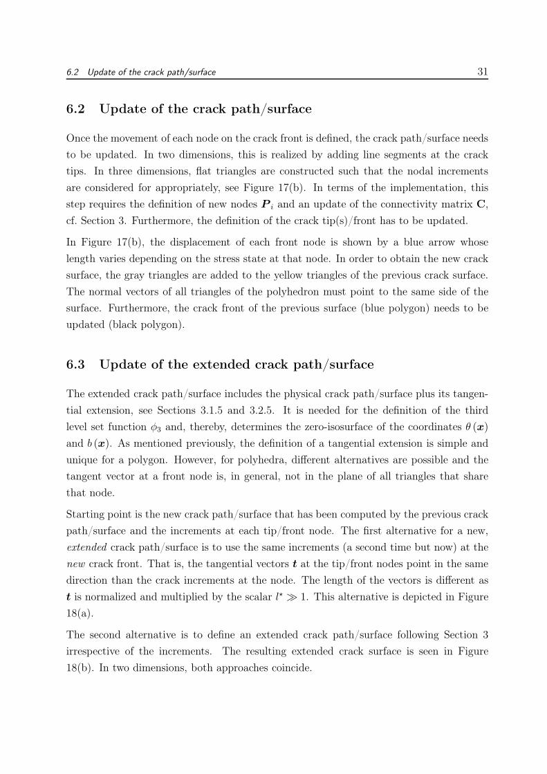
(a) Approach 1. (b) Approach 2.

Figure 18: New extended crack surfaces by the two different approaches. The yellowtriangles constitute the previous crack surface. The new crack surface that considers theincrements of different length (blue arrows) at each node also includes the gray triangles.The extended new surface is based on normalized tangential vectors multiplied by the scalarl⋆ = 3 (black arrows) and involves also the orange triangles. In practice, l⋆ is larger andensures that the extended crack surface completely intersects the domain.

It is noted that, in general, the two approaches yield very similar results, compare 18(a) and

(b). We found, however, that the second approach is more robust in situations where the

crack increments have very different lengths at the crack front. In particular, for increments

that are close to zero one may obtain a useful new crack surface but the extended new

crack surface through approach 1 may be less satisfactory. Approach 2 has typically a

smoothing influence on the extended crack surface and is, therefore, recommended.

7 Numerical results

Test cases in linear elastic fracture mechanics (LEFM) are presented in two and three

dimensions. LEFM is suitable for the simulation of crack growth in brittle materials; only

quasi-static crack growth is considered in this work. The governing equations of linear

elasticity are given in a numerous number of basic engineering books [8, 41] and are omitted

here for brevity. It is noted that our interest in this work is only in the crack propagation

based on the method presented above; no stress intensity factors, energy release rates,

fracture toughness, models for crack initiation, etc. are needed. Furthermore, we mention

that the method has also proven its usefulness for cohesive cracks. Then, one may not

want to employ the crack-tip enrichments of section 5.4 but the scheme proposed herein

is still useful in order to avoid the implementation of additional models for the level-set

7.1 Crack propagation in two dimensions 33

update, see e.g. [36, 64].

In the two-dimensional test-cases, it is shown that the proposed description of the cracks is

valid for edge cracks, immersed cracks, and also multiple cracks. Furthermore, the model

for the crack propagation is investigated with respect to tension, bending, and shearing.

Thereafter, the extension to three dimensions is realized. One test case is a pseudo-3d-

problem and results are compared with the two-dimensional situation. Thereafter, two

additional test cases are considered that do not allow for a simplification to two dimensions.

7.1 Crack propagation in two dimensions

7.1.1 Tension and shearing in a unit-square specimen

0.5 0.5

1

0.50.5

1

α

α

x

y

(a) Dimensions and supports. (b) Mesh.

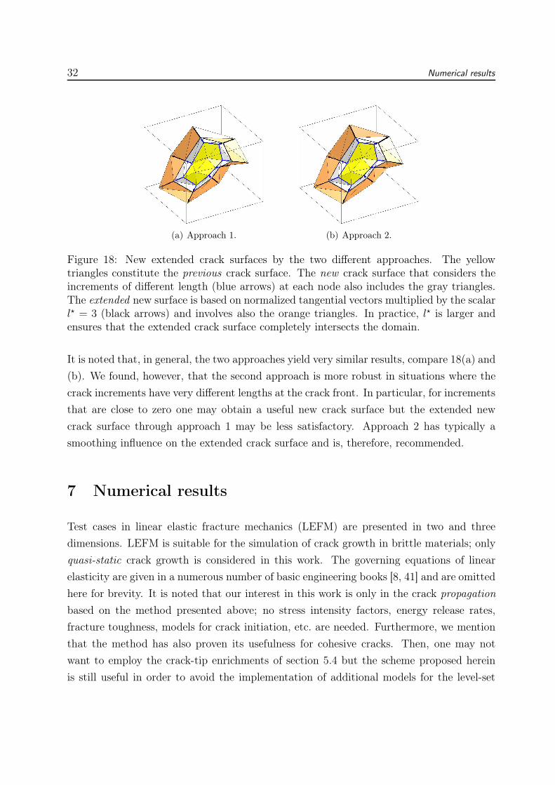
Figure 19: Test case with one edge crack in a unit-square specimen.

The first test case considers a unit-square domain with an initial edge crack that goes

from the center of the domain horizontally to the left side of the domain, see Figure

19(a). Similar settings are studied e.g. in [17]. Asymmetric boundary conditions for the

displacement are prescribed on the upper and lower side of the domain. The displacements

are specified by an angle α. For α = 90, the load is dominated by tension. For α = 0 or

180, the boundary conditions imply a shear loading. In all situations, Young’s modulus

is E = 3 · 107, Poisson’s ratio ν = 0.3, and plane strain conditions are adopted.

The domain is discretized by a structured mesh, see Figure 19(b). The initial crack is not

meshed explicitly but given as one segment of the polygon. Only the right node of the


segment represents the (active) crack tip. The left point of the segment does not have to

be part of the domain but could be placed further to the left. Each propagation step adds

one segment to the crack.

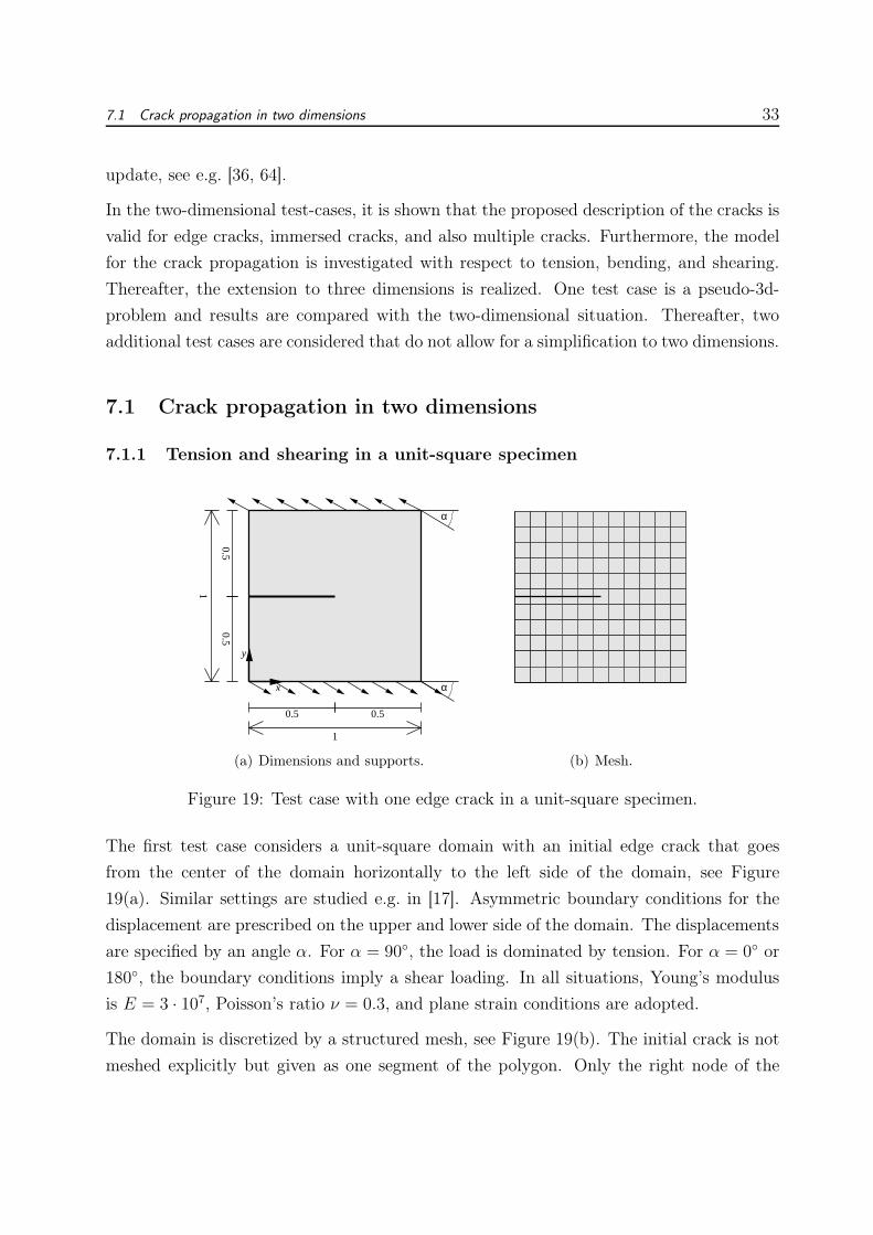
In the first part of the study we use α = 30 and systematically vary the radius of the

stress circle rc, the size of the crack increment da, and number of elements. Figure 20(a)

shows the crack paths for different rc = 0.05, 0.025, 0.01, 0.005, 0.001 and a constant

increment of da = 0.025 and 41 × 41 elements. It is seen that for the whole range of rc,

very similar paths are obtained. In Figure 20(b), paths are shown for different increments,

da = 0.05, 0.025, 0.0125, 0.00625, a constant rc = 0.01 and 41 × 41 elements. Again,

the paths are very similar. Finally, Figure 20(c) depicts results for an increasing number

of elements per dimension, 11, 21, 41, 81, and keeps rc = 0.00625 and da = 0.00625

constant. It is seen that the method allows to specify the domain discretization and the

crack discretization with great flexibility. For the last setting, the increment is so small

that about 80 steps are needed until the domain is almost cut, nevertheless, only 11× 11

elements are used. Also the opposite statement is true: One may, in general, obtain stable

and useful results for very fine meshes but with coarse increments. Obviously, for an

“optimal” convergence, the mesh and crack discretization should be coupled so that fine

meshes and small increments come together. We conclude, that for this test case, accurate

results are found for a large variety of radii rc, increments da, and number of elements. It

shall be seen later that more complex test cases are more restrictive with respect to the

choice of these parameters.

(a) Variation of rc. (b) Variation of da. (c) Variation of the elementnumber.

Figure 20: Resulting crack paths for α = 30.

In the second part of the study, the influence of the complete range of angles 0 ≤ α ≤ 180

of the prescribed displacements on the upper and lower wall on the crack path is studied.

Therefore, we use rc = 0.025, da = 0.025, and 81× 81 elements. The results are shown in


α = 0°, 180°α = 15°, 165°α = 30°, 180°α = 45°, 135°α = 60°, 120°α = 75°, 105°α = 90°

(a)

−70−60

−50

−40

−30

−20

−10

0

10

20

3040

50

60

70

(b) Detail.

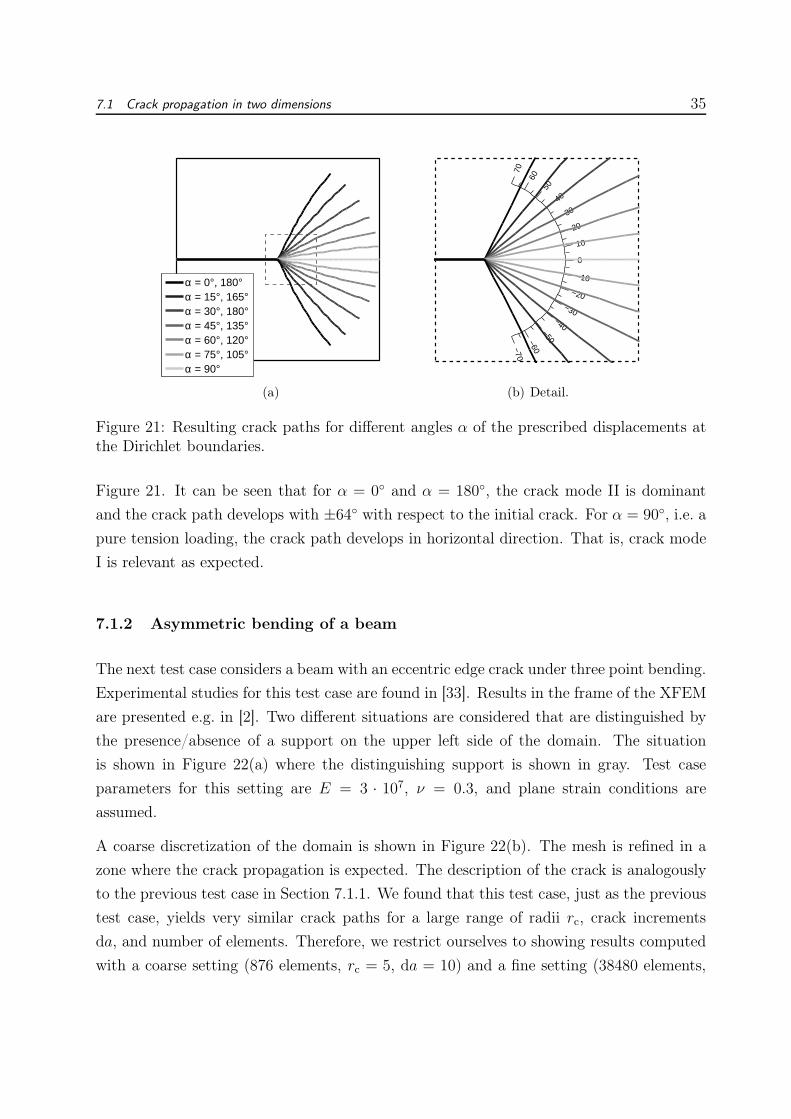
Figure 21: Resulting crack paths for different angles α of the prescribed displacements atthe Dirichlet boundaries.

Figure 21. It can be seen that for α = 0 and α = 180, the crack mode II is dominant

and the crack path develops with ±64 with respect to the initial crack. For α = 90, i.e. a

pure tension loading, the crack path develops in horizontal direction. That is, crack mode

I is relevant as expected.

7.1.2 Asymmetric bending of a beam

The next test case considers a beam with an eccentric edge crack under three point bending.

Experimental studies for this test case are found in [33]. Results in the frame of the XFEM

are presented e.g. in [2]. Two different situations are considered that are distinguished by

the presence/absence of a support on the upper left side of the domain. The situation

is shown in Figure 22(a) where the distinguishing support is shown in gray. Test case

parameters for this setting are E = 3 · 107, ν = 0.3, and plane strain conditions are

assumed.

A coarse discretization of the domain is shown in Figure 22(b). The mesh is refined in a

zone where the crack propagation is expected. The description of the crack is analogously

to the previous test case in Section 7.1.1. We found that this test case, just as the previous

test case, yields very similar crack paths for a large range of radii rc, crack increments

da, and number of elements. Therefore, we restrict ourselves to showing results computed

with a coarse setting (876 elements, rc = 5, da = 10) and a fine setting (38480 elements,


rc = 0.5, da = 1.0). More systematic studies on these parameters are shown below for

more complex test cases.

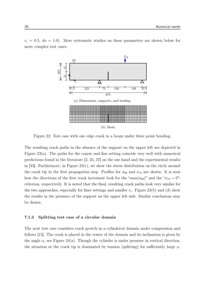
F

37.5 225 75 150 150 37.5

675

7575

150

x

y

(a) Dimensions, supports, and loading.

(b) Mesh.

Figure 22: Test case with one edge crack in a beam under three point bending.

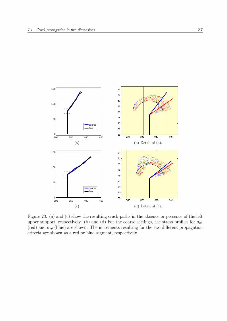
The resulting crack paths in the absence of the support on the upper left are depicted in

Figure 23(a). The paths for the coarse and fine setting coincide very well with numerical

predictions found in the literature [2, 25, 37] on the one hand and the experimental results

in [33]. Furthermore, in Figure 23(c), we show the stress distribution on the circle around

the crack tip in the first propagation step. Profiles for σθθ and σrθ are shown. It is seen

how the directions of the first crack increment look for the “max(σθθ)” and the “σrθ = 0”-

criterion, respectively. It is noted that the final, resulting crack paths look very similar for

the two approaches, especially for finer settings and smaller rc. Figure 23(b) and (d) show

the results in the presence of the support on the upper left side. Similar conclusions may

be drawn.

7.1.3 Splitting test case of a circular domain

The next test case considers crack growth in a cylindrical domain under compression and

follows [15]. The crack is placed in the center of the domain and its inclination is given by

the angle α, see Figure 24(a). Though the cylinder is under pressure in vertical direction,

the situation at the crack tip is dominated by tension (splitting) for sufficiently large α.


300 350 400 4500

50

100

150

coarsefine

(a) (b) Detail of (a).

300 350 400 4500

50

100

150

coarsefine

(c) (d) Detail of (c).

Figure 23: (a) and (c) show the resulting crack paths in the absence or presence of the leftupper support, respectively. (b) and (d) For the coarse settings, the stress profiles for σθθ(red) and σrθ (blue) are shown. The increments resulting for the two different propagationcriteria are shown as a red or blue segment, respectively.


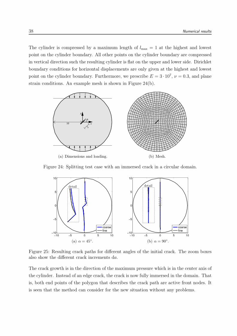
The cylinder is compressed by a maximum length of lmax = 1 at the highest and lowest

point on the cylinder boundary. All other points on the cylinder boundary are compressed

in vertical direction such the resulting cylinder is flat on the upper and lower side. Dirichlet

boundary conditions for horizontal displacements are only given at the highest and lowest

point on the cylinder boundary. Furthermore, we prescribe E = 3 · 107, ν = 0.3, and plane

strain conditions. An example mesh is shown in Figure 24(b).

10

2

αx

y

(a) Dimensions and loading. (b) Mesh.

Figure 24: Splitting test case with an immersed crack in a circular domain.

(a) α = 45. (b) α = 90.

Figure 25: Resulting crack paths for different angles of the initial crack. The zoom boxesalso show the different crack increments da.

The crack growth is in the direction of the maximum pressure which is in the center axis of

the cylinder. Instead of an edge crack, the crack is now fully immersed in the domain. That

is, both end points of the polygon that describes the crack path are active front nodes. It

is seen that the method can consider for the new situation without any problems.


Also this test case is not very restrictive on the choice of the parameters rc and da. There-

fore, only a coarse setting with 2352 elements, rc = 0.5, da = 1 and a fine setting with

37632 elements, rc = 0.0625, da = 0.125 are compared. Resulting crack paths for two dif-

ferent angles of α are seen in Figure 25. Again, coarse and fine settings yield very similar

results which are in very good agreement to the results presented e.g. in [15].

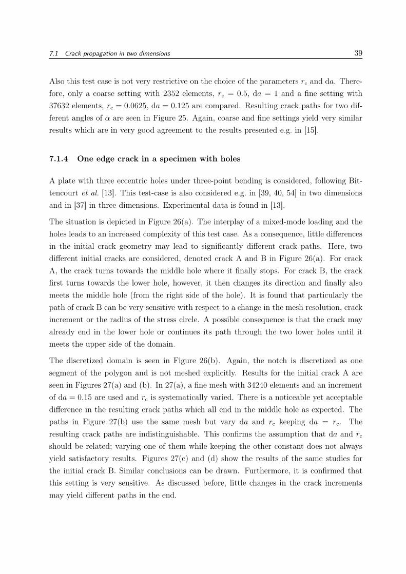
7.1.4 One edge crack in a specimen with holes

A plate with three eccentric holes under three-point bending is considered, following Bit-

tencourt et al. [13]. This test-case is also considered e.g. in [39, 40, 54] in two dimensions

and in [37] in three dimensions. Experimental data is found in [13].

The situation is depicted in Figure 26(a). The interplay of a mixed-mode loading and the

holes leads to an increased complexity of this test case. As a consequence, little differences

in the initial crack geometry may lead to significantly different crack paths. Here, two

different initial cracks are considered, denoted crack A and B in Figure 26(a). For crack

A, the crack turns towards the middle hole where it finally stops. For crack B, the crack

first turns towards the lower hole, however, it then changes its direction and finally also

meets the middle hole (from the right side of the hole). It is found that particularly the

path of crack B can be very sensitive with respect to a change in the mesh resolution, crack

increment or the radius of the stress circle. A possible consequence is that the crack may

already end in the lower hole or continues its path through the two lower holes until it

meets the upper side of the domain.

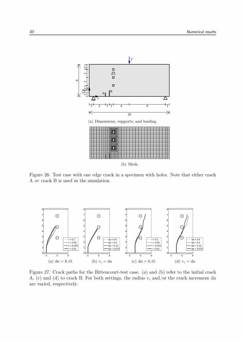
The discretized domain is seen in Figure 26(b). Again, the notch is discretized as one

segment of the polygon and is not meshed explicitly. Results for the initial crack A are

seen in Figures 27(a) and (b). In 27(a), a fine mesh with 34240 elements and an increment

of da = 0.15 are used and rc is systematically varied. There is a noticeable yet acceptable

difference in the resulting crack paths which all end in the middle hole as expected. The

paths in Figure 27(b) use the same mesh but vary da and rc keeping da = rc. The

resulting crack paths are indistinguishable. This confirms the assumption that da and rc

should be related; varying one of them while keeping the other constant does not always

yield satisfactory results. Figures 27(c) and (d) show the results of the same studies for

the initial crack B. Similar conclusions can be drawn. Furthermore, it is confirmed that

this setting is very sensitive. As discussed before, little changes in the crack increments

may yield different paths in the end.


F

0.5

1 3 1 1 4 9 1

20

1.252

21.250.5 1

8

AB

x

y

(a) Dimensions, supports, and loading.

(b) Mesh.

Figure 26: Test case with one edge crack in a specimen with holes. Note that either crackA or crack B is used in the simulation.

4 6 80

1

2

3

4

5

6

7

8

r = 0.1r = 0.05r = 0.025r = 0.01

(a) da = 0.15

4 6 80

1

2

3

4

5

6

7

8

da = 0.6da = 0.3da = 0.15da = 0.075

(b) rc = da

4 6 80

1

2

3

4

5

6

7

8

r = 0.1r = 0.05r = 0.025r = 0.01

(c) da = 0.15

4 6 80

1

2

3

4

5

6

7

8

da = 0.6da = 0.3da = 0.15da = 0.075

(d) rc = da

Figure 27: Crack paths for the Bittencourt-test case. (a) and (b) refer to the initial crackA, (c) and (d) to crack B. For both settings, the radius rc and/or the crack increment daare varied, respectively.


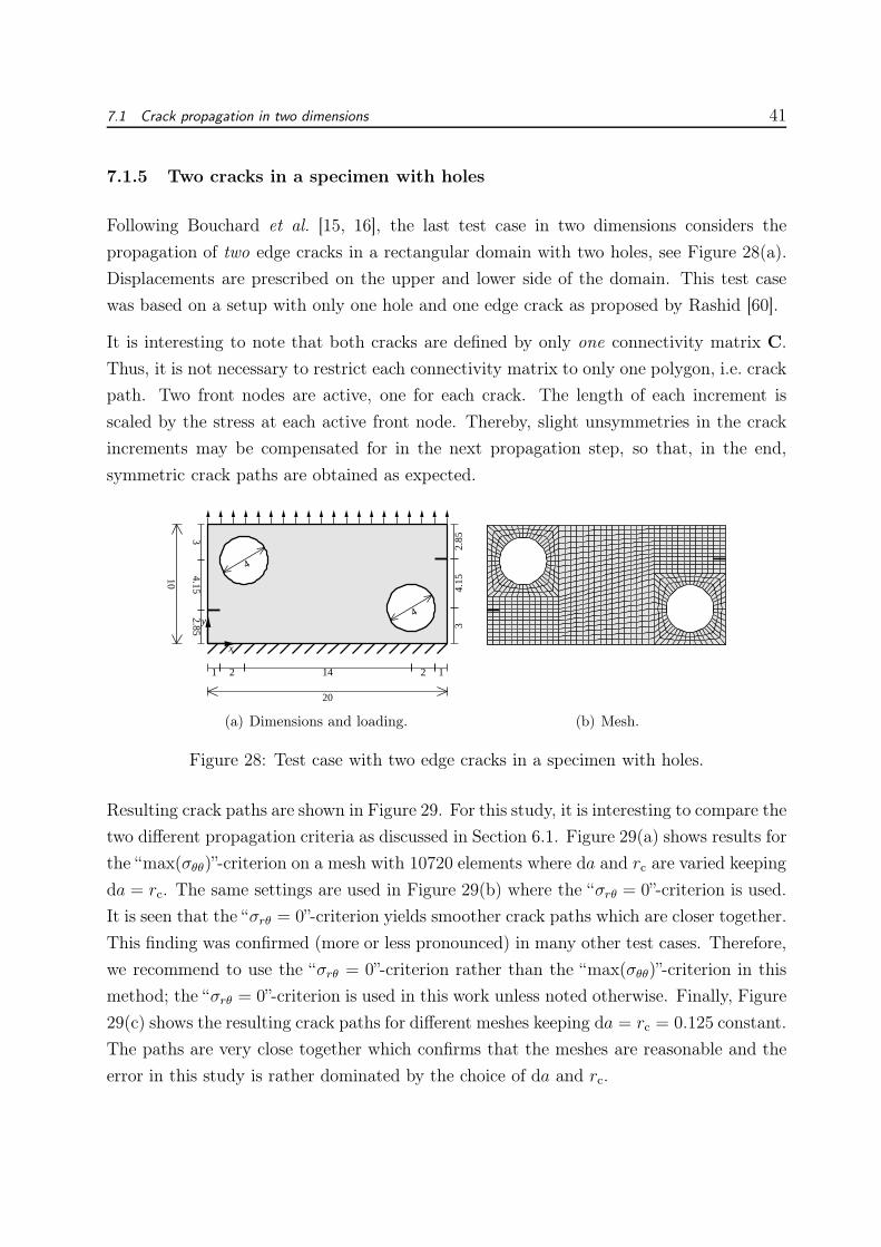
7.1.5 Two cracks in a specimen with holes

Following Bouchard et al. [15, 16], the last test case in two dimensions considers the

propagation of two edge cracks in a rectangular domain with two holes, see Figure 28(a).

Displacements are prescribed on the upper and lower side of the domain. This test case

was based on a setup with only one hole and one edge crack as proposed by Rashid [60].

It is interesting to note that both cracks are defined by only one connectivity matrix C.

Thus, it is not necessary to restrict each connectivity matrix to only one polygon, i.e. crack

path. Two front nodes are active, one for each crack. The length of each increment is

scaled by the stress at each active front node. Thereby, slight unsymmetries in the crack

increments may be compensated for in the next propagation step, so that, in the end,

symmetric crack paths are obtained as expected.

1 2 14 2 1

203

4.152.85 3

4.15

2.85

10

4

4

x

y

(a) Dimensions and loading. (b) Mesh.

Figure 28: Test case with two edge cracks in a specimen with holes.

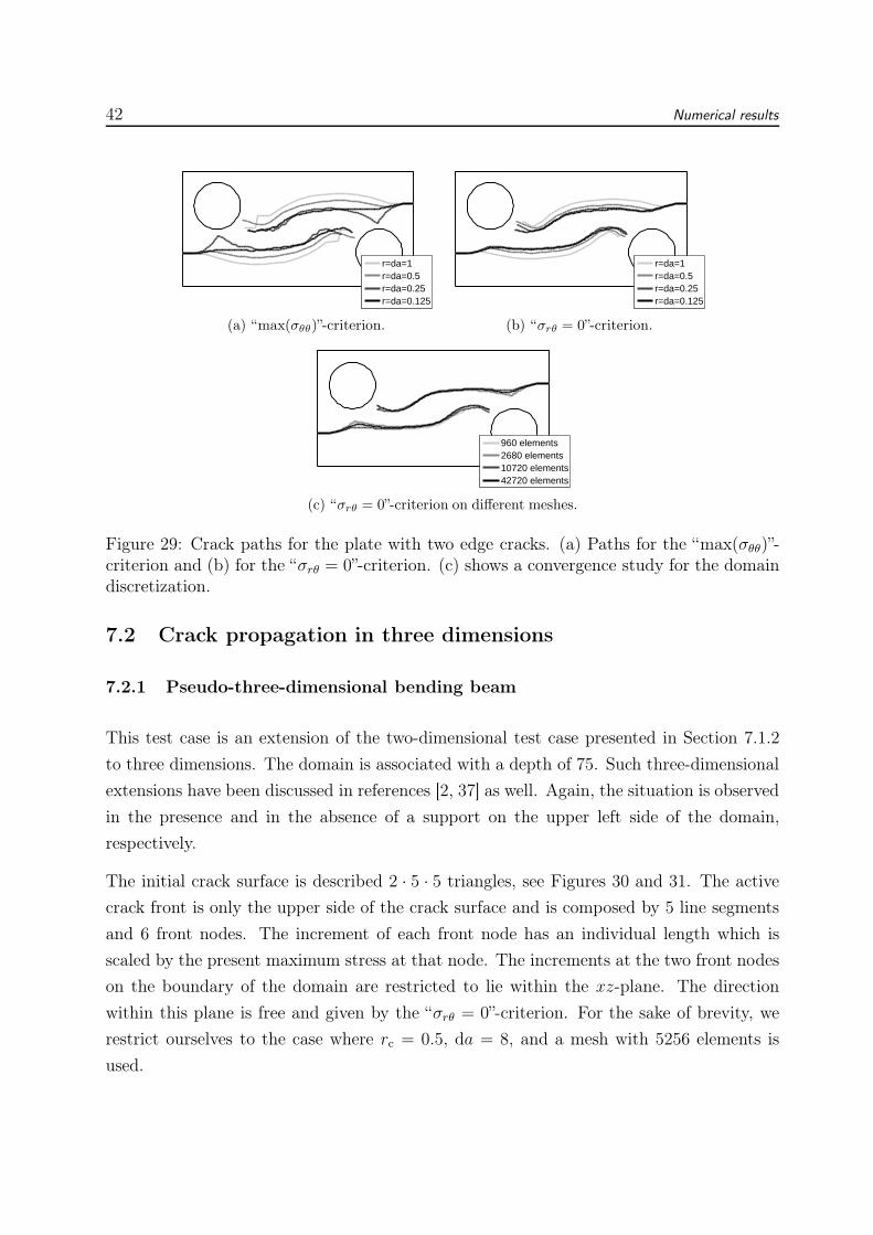
Resulting crack paths are shown in Figure 29. For this study, it is interesting to compare the

two different propagation criteria as discussed in Section 6.1. Figure 29(a) shows results for

the “max(σθθ)”-criterion on a mesh with 10720 elements where da and rc are varied keeping

da = rc. The same settings are used in Figure 29(b) where the “σrθ = 0”-criterion is used.

It is seen that the “σrθ = 0”-criterion yields smoother crack paths which are closer together.

This finding was confirmed (more or less pronounced) in many other test cases. Therefore,

we recommend to use the “σrθ = 0”-criterion rather than the “max(σθθ)”-criterion in this

method; the “σrθ = 0”-criterion is used in this work unless noted otherwise. Finally, Figure

29(c) shows the resulting crack paths for different meshes keeping da = rc = 0.125 constant.

The paths are very close together which confirms that the meshes are reasonable and the

error in this study is rather dominated by the choice of da and rc.


r=da=1r=da=0.5r=da=0.25r=da=0.125

(a) “max(σθθ)”-criterion.

r=da=1r=da=0.5r=da=0.25r=da=0.125

(b) “σrθ = 0”-criterion.

960 elements2680 elements10720 elements42720 elements

(c) “σrθ = 0”-criterion on different meshes.

Figure 29: Crack paths for the plate with two edge cracks. (a) Paths for the “max(σθθ)”-criterion and (b) for the “σrθ = 0”-criterion. (c) shows a convergence study for the domaindiscretization.

7.2 Crack propagation in three dimensions

7.2.1 Pseudo-three-dimensional bending beam

This test case is an extension of the two-dimensional test case presented in Section 7.1.2

to three dimensions. The domain is associated with a depth of 75. Such three-dimensional

extensions have been discussed in references [2, 37] as well. Again, the situation is observed

in the presence and in the absence of a support on the upper left side of the domain,

respectively.

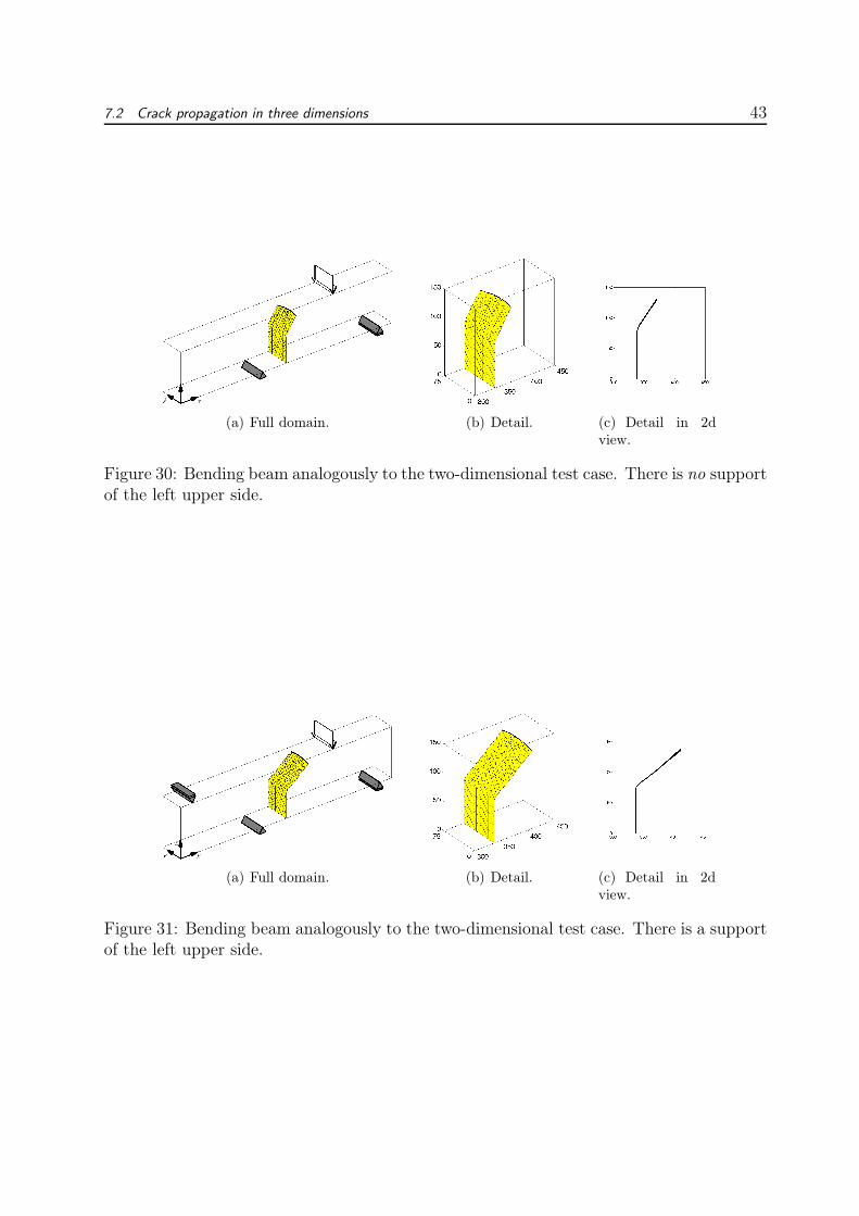
The initial crack surface is described 2 · 5 · 5 triangles, see Figures 30 and 31. The active

crack front is only the upper side of the crack surface and is composed by 5 line segments

and 6 front nodes. The increment of each front node has an individual length which is

scaled by the present maximum stress at that node. The increments at the two front nodes

on the boundary of the domain are restricted to lie within the xz-plane. The direction

within this plane is free and given by the “σrθ = 0”-criterion. For the sake of brevity, we

restrict ourselves to the case where rc = 0.5, da = 8, and a mesh with 5256 elements is

used.

7.2 Crack propagation in three dimensions 43

(a) Full domain. (b) Detail. (c) Detail in 2dview.

Figure 30: Bending beam analogously to the two-dimensional test case. There is no supportof the left upper side.

(a) Full domain. (b) Detail. (c) Detail in 2dview.

Figure 31: Bending beam analogously to the two-dimensional test case. There is a supportof the left upper side.


Results for the case where no support on the upper left side is present, are shown in Figure

30. The front view of the crack surface in Figure 30(c) shows that a perfect match with the

two-dimensional solution is obtained, cf. Figure 23, and that the whole surface stays flat

in y-direction as expected. Figure 31 confirms these finding in the presence of a support

on the upper left side.

7.2.2 Prismatic beam under torsion

Following the experimental studies by Brokenshire [18], a beam with a skew crack is sub-

jected to torsion. Simulations in the frame of the XFEM are presented by Gasser and

Holzapfel [32] and Gürses and Miehe [37]. A sketch of the situation is seen in Figure 32.

It is seen that a full three-dimensional study of this test case is required as no reduction

to two dimensions is possible.

The initial crack surface is described 2 · 15 · 15 triangles resulting in 15 line segments along

the crack front. In this case, all inner nodes on the crack front may freely move. It is

recalled that in each step, the movement is limited to the plane spanned by the normal

and tangential vector at that node. But from one iteration step to the next, the plane can

reorient so that the final motion of a front node is, in this sense, free. Only the movement of

the outer front nodes is restricted to the yz-plane which coincides with the outer boundary

of the beam. For this test case, we choose E = 3 · 107 and ν = 0.3 for the inner part

of the beam. The two prismatic bodies at the two ends of the beams are assumed to be

rigid bodies. The beam is fixed at three of the tips of the prismatic bodies. A rotation of

α = 10 in the yz-plane is applied around the left back tip node.

Results for a mesh with 12840 elements, rc = 1, and da = 5 are shown in Figure 33. It is

seen that the crack surface develops in a complex motion which is also found in [32, 37].

It is noted that the crack front is very smooth compared to other studies. Furthermore,

the angle of the surface at the two sides of the beam is larger than those in other studies,

see Figure 33(c).

7.2.3 Plate under impact

The final test case considered in this work is motivated from the Kalthoff experiment in

[44]. Numerical studies using the classical FEM are found in Batra and Ravinsankar [5],

meshfree methods are employed in Rabczuk et al. [56], and XFEM-results are presented in

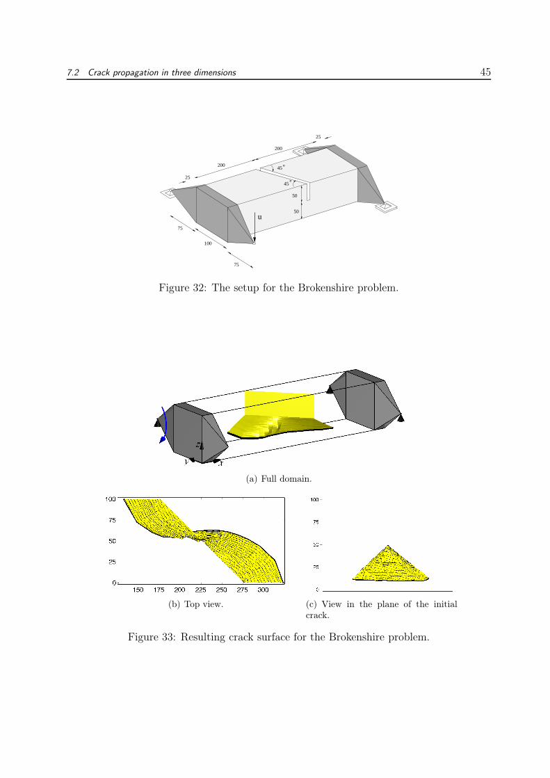
7.2 Crack propagation in three dimensions 45

u

50

50

75

75

100

200

200

25

25

45°

45°

Figure 32: The setup for the Brokenshire problem.

(a) Full domain.

(b) Top view. (c) View in the plane of the initialcrack.

Figure 33: Resulting crack surface for the Brokenshire problem.

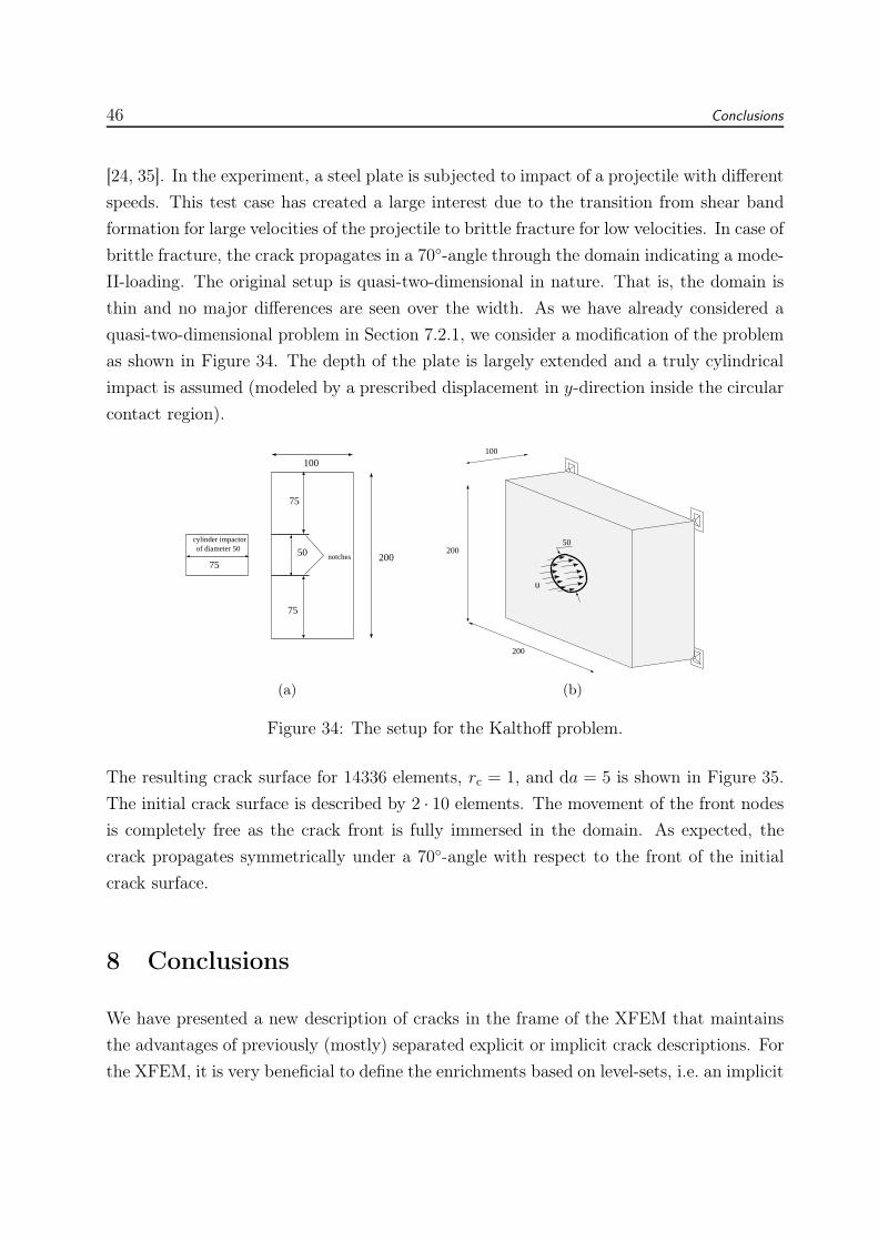
46 Conclusions

[24, 35]. In the experiment, a steel plate is subjected to impact of a projectile with different

speeds. This test case has created a large interest due to the transition from shear band

formation for large velocities of the projectile to brittle fracture for low velocities. In case of

brittle fracture, the crack propagates in a 70-angle through the domain indicating a mode-

II-loading. The original setup is quasi-two-dimensional in nature. That is, the domain is

thin and no major differences are seen over the width. As we have already considered a

quasi-two-dimensional problem in Section 7.2.1, we consider a modification of the problem

as shown in Figure 34. The depth of the plate is largely extended and a truly cylindrical

impact is assumed (modeled by a prescribed displacement in y-direction inside the circular

contact region).

notches50

100

200

75

75

75

cylinder impactorof diameter 50

(a)

200

200

100

50

u

(b)

Figure 34: The setup for the Kalthoff problem.

The resulting crack surface for 14336 elements, rc = 1, and da = 5 is shown in Figure 35.

The initial crack surface is described by 2 · 10 elements. The movement of the front nodes

is completely free as the crack front is fully immersed in the domain. As expected, the

crack propagates symmetrically under a 70-angle with respect to the front of the initial

crack surface.

8 Conclusions

We have presented a new description of cracks in the frame of the XFEM that maintains

the advantages of previously (mostly) separated explicit or implicit crack descriptions. For

the XFEM, it is very beneficial to define the enrichments based on level-sets, i.e. an implicit

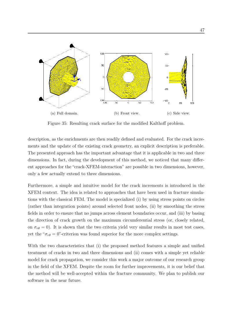
47

(a) Full domain. (b) Front view. (c) Side view.

Figure 35: Resulting crack surface for the modified Kalthoff problem.

description, as the enrichments are then readily defined and evaluated. For the crack incre-

ments and the update of the existing crack geometry, an explicit description is preferable.

The presented approach has the important advantage that it is applicable in two and three

dimensions. In fact, during the development of this method, we noticed that many differ-

ent approaches for the “crack-XFEM-interaction” are possible in two dimensions, however,

only a few actually extend to three dimensions.

Furthermore, a simple and intuitive model for the crack increments is introduced in the

XFEM context. The idea is related to approaches that have been used in fracture simula-

tions with the classical FEM. The model is specialized (i) by using stress points on circles

(rather than integration points) around selected front nodes, (ii) by smoothing the stress

fields in order to ensure that no jumps across element boundaries occur, and (iii) by basing

the direction of crack growth on the maximum circumferential stress (or, closely related,

on σrθ = 0). It is shown that the two criteria yield very similar results in most test cases,

yet the “σrθ = 0”-criterion was found superior for the more complex settings.

With the two characteristics that (i) the proposed method features a simple and unified

treatment of cracks in two and three dimensions and (ii) comes with a simple yet reliable

model for crack propagation, we consider this work a major outcome of our research group

in the field of the XFEM. Despite the room for further improvements, it is our belief that

the method will be well-accepted within the fracture community. We plan to publish our

software in the near future.

48 REFERENCES

Acknowledgements

The support of the German Research Foundation (DFG) in the frame of the Emmy-

Noether-research group “Numerical methods for discontinuities in continuum mechanics”

is gratefully acknowledged.

References

[1] Anderson, T.L.: Fracture Mechanics: Fundamentals and Applications. CRC Press,

Boca Raton, 2005.

[2] Areias, P.M.A.; Belytschko, T.: Analysis of three-dimensional crack initiation and

propagation using the extended finite element method. Internat. J. Numer. Methods

Engrg., 63, 760 – 788, 2005.

[3] Bærentzen, J.A.: Robust Generation of Signed Distance Fields from Triangle Meshes.

Volume Graphics, 11, 167 – 175, 2005.

[4] Bærentzen, J.A.; Aanæs, H.: Signed distance computation using the angle weighted

pseudo-normal. Transactions on Visualization and Computer Graphics, 11, 243 – 253,

2005.

[5] Batra, R.C.; Ravinsankar, M.V.S.: Three-dimensional numerical simulation of the

Kalthoff experiment. Int. J. of Fracture, 105, 161 – 186, 2000.

[6] Belytschko, T.; Black, T.: Elastic crack growth in finite elements with minimal remesh-

ing. Internat. J. Numer. Methods Engrg., 45, 601 – 620, 1999.

[7] Belytschko, T.; Krongauz, Y.; Organ, D.; Fleming, M.; Krysl, P.: Meshless Methods:

An Overview and Recent Developments. Comp. Methods Appl. Mech. Engrg., 139, 3

– 47, 1996.

[8] Belytschko, T.; Liu, W.K.; Moran, B.: Nonlinear Finite Elements for Continua and

Structures. John Wiley & Sons, Chichester, 2000.

[9] Belytschko, T.; Lu, Y.Y.; Gu, L.: Crack propagation by element-free Galerkin meth-

ods. Engrg. Fract. Mech., 51, 295 – 315, 1995.

REFERENCES 49

[10] Belytschko, T.; Lu, Y.Y.; Gu, L.; Tabbara, M.: Element-free Galerkin methods for

static and dynamic fracture. Int. J. Solids Struct., 32, 2547 – 2570, 1995.

[11] Belytschko, T.; Moës, N.; Usui, S.; Parimi, C.: Arbitrary discontinuities in finite

elements. Internat. J. Numer. Methods Engrg., 50, 993 – 1013, 2001.

[12] Belytschko, T.; Parimi, C.; Moës, N.; Sukumar, N.; Usui, S.: Structured extended

finite element methods for solids defined by implicit surfaces. Internat. J. Numer.

Methods Engrg., 56, 609 – 635, 2003.

[13] Bittencourt, T.N.; Wawrzynek, P.A.; Ingraffea, A.R.; Sousa, J.L.: Quasi-automatic

simulation of crack propagation for 2D LEFM problems. Engineering Fracture Me-

chanics, 55, 321 – 334, 1996.

[14] Bloomenthal, J.; Bajaj, C.; Blinn, J.; Cani-Gascuel, M.P.; Rockwood, A.; Wyvill,

B.; Wyvill, G.: Introduction to Implicit Surfaces. Morgan Kaufmann Publishers, San

Francisco, 1997.

[15] Bouchard, Pierre Olivier: Contribution á la modélisation numérique en mécanique de

la rupture et structures multimatériaux. Phd thesis, Ecole Nationale Supérieure des

Mines de Paris, France, 2000.

[16] Bouchard, P.O.; Bay, F.; Chastel, Y.: Numerical modelling of crack propagation:

automatic remeshing and comparison of different criteria. Comp. Methods Appl. Mech.

Engrg., 192, 3887 – 3908, 2003.

[17] Bourdin, B.: Une formulation variationnelle en mécanique de la rupture, théorie et

mise en oeuvre numérique. Phd thesis, Université Paris Nord, France, 1998.

[18] Brokenshire, D.R.: Torsional fracture tests. Phd thesis, Cardiff University, UK, 2007.

[19] Cheng, K.W.; Fries, T.P.: Higher-order XFEM for curved strong and weak disconti-

nuities. Internat. J. Numer. Methods Engrg., 82, 564 – 590, 2010.

[20] Cherepanov, G.P.: The propagation of cracks in a continuous medium. J. of Applied

Mechanincs and Mathematics, 31, 503 – 512, 1967.

[21] Chessa, J.; Wang, H.; Belytschko, T.: On the construction of blending elements for

local partition of unity enriched finite elements. Internat. J. Numer. Methods Engrg.,

57, 1015 – 1038, 2003.

50 REFERENCES

[22] Daux, C.; Moës, N.; Dolbow, J.; Sukumar, N.; Belytschko, T.: Arbitrary branched

and intersecting cracks with the extended finite element method. Internat. J. Numer.

Methods Engrg., 48, 1741 – 1760, 2000.

[23] Duarte, C.A.; Hamzeh, O.N.; Liszka, T.J.; Tworzydlo, W.W.: A generalized finite

element method for the simulation of three-dimensional dynamic crack propagation.

Comp. Methods Appl. Mech. Engrg., 190, 2227 – 2262, 2001.

[24] Elguedj, T.; Gravouil, A.; Maigre, H.: An explicit dynamics extended finite element

method. Part 1: Mass lumping for arbitrary enrichment functions. Comp. Methods

Appl. Mech. Engrg., 198, 2297 – 2317, 2009.

[25] Erdogan, F.; Sih, G.: On the crack extension in plates under plane loading and

transverse shear. Journal of Basic Engineering, 85, 519 – 527, 1963.

[26] Eshelby, J.D.: The force on an elastic singularity. Philosophical transactions of the

Royal Society of London, 244, 27 – 112, 1951.

[27] Fries, T.P.: A corrected XFEM approximation without problems in blending elements.

Internat. J. Numer. Methods Engrg., 75, 503 – 532, 2008.

[28] Fries, T.P.; Belytschko, T.: The extended/generalized finite element method: An

overview of the method and its applications. Internat. J. Numer. Methods Engrg., 84,

253 – 304, 2010.

[29] Fries, T.P.; Byfut, A.; Alizada, A.; Cheng, K.W.; Schröder, A.: Hanging nodes and

XFEM. Internat. J. Numer. Methods Engrg., 86, 404 – 430, 2011.

[30] Fries, T.P.; Matthies, H.G.: Classification and Overview of Meshfree Methods.

Informatikbericht-Nr. 2003-03, Technical University Braunschweig, (http://opus.tu-

bs.de/opus/volltexte/2003/418/), Brunswick, 2003.

[31] Fries, T.P.; Moës, N.; (editors), A. Zilian: The extended finite element method, special

issue. Internat. J. Numer. Methods Engrg., 86, 403 – 666, 2011.

[32] Gasser, T.C; Holzapfel, G.A.: Modeling 3D crack propagation in unreinforced concrete

using PUFEM. Comp. Methods Appl. Mech. Engrg., 194, 2859 – 2896, 2005.

[33] Glávez, J.C.; Elices, M.; Guinea, G.V.; Planas, J.: Fracture of concrete under propo-

tional and nonproportional loading. Int. J. of Fracture, 94, 267 – 284, 1998.

REFERENCES 51

[34] Gracie, R.; Wang, H.; Belytschko, T.: Blending in the extended finite element method

by discontinuous Galerkin and assumed strain methods. Internat. J. Numer. Methods

Engrg., 74, 1645 – 1669, 2008.

[35] Gravouil, A.; Elguedj, T.; Maigre, H.: An explicit dynamics extended finite element

method. Part 2: Element-by-element stable-explicit/explicit dynamic scheme. Comp.

Methods Appl. Mech. Engrg., 198, 2318 – 2328, 2009.

[36] Gravouil, A.; Moës, N.; Belytschko, T.: Non-planar 3D crack growth by the extended

finite element and level sets, part II: level set update. Internat. J. Numer. Methods

Engrg., 53, 2569 – 2586, 2002.

[37] Gürses, E.; Miehe, C.: A computational framework of three-dimensional

configurational-force-driven brittle crack propagation. Comp. Methods Appl. Mech.

Engrg., 198, 1413 – 1428, 2009.

[38] Gurtin, M.E.: The nature of configurational forces. Archive for Rational Mechanics

and Analysis, 131, 67 – 100, 1995.

[39] Häusler, S.M.; Lindhorst, K.; Horst, P.: Combination of the material force concept

and the extended finite element method for mixed mode crack simulations. Internat.

J. Numer. Methods Engrg., 85, 1522 – 1542, 2011.

[40] Heintz, P.: On the numerical modelling of quasi static crack growth in linear elastic

fracture mechanics. Internat. J. Numer. Methods Engrg., 65, 174 – 189, 2006.

[41] Hughes, T.J.R.: The Finite Element Method: Linear Static and Dynamic Finite Ele-

ment Analysis. Prentice-Hall, Englewood Cliffs, NJ, 1987.

[42] Ingraffea, A.R.: Computational Fracture Mechanics. In Encyclopedia of Computa-

tional Mechanics. (E. Stein, R. de Borst, T.J.R. Hughes, Ed.), Vol. 2, John Wiley &

Sons, Chichester, 2007.

[43] Irwin, G.R.: Analysis of stresses and strains near the end of a crack traversing a plate.

J. Appl. Mech., ASME, 24, 361 – 364, 1957.

[44] Kalthoff, J.F.; Winkler, S.: Failure mode transition at high rates of shear loading.

Impact Loading and Dynamic Behavior of Materials, 1, 185 – 195, 1987.

52 REFERENCES

[45] Karihaloo, B.L.; Xiao, Q.Z.: Modelling of stationary and growing cracks in FE frame-

work without remeshing: a state-of-the-art review. Computers & Structures, 81, 119

– 129, 2003.

[46] Krysl, P.; Belytschko, T.: The element free Galerkin method for dynamic propagation

of arbitrary 3-D cracks. Internat. J. Numer. Methods Engrg., 44, 767 – 800, 1999.

[47] Laborde, P.; Pommier, J.; Renard, Y.; Salaün, M.: High-order extended finite element

method for cracked domains. Internat. J. Numer. Methods Engrg., 64, 354 – 381, 2005.

[48] Maiti, S.K.; Smith, R.A.: Comparison of the criteria for mixed mode brittle fracture

based on the preinstability stress–strain field. Part II: pure shear and uniaxial loading.

Int. J. of Fracture, 24, 5 – 22, 1984.

[49] Moës, N.; Dolbow, J.; Belytschko, T.: A finite element method for crack growth

without remeshing. Internat. J. Numer. Methods Engrg., 46, 131 – 150, 1999.

[50] Moës, N.; Gravouil, A.; Belytschko, T.: Non-planar 3D crack growth by the extended

finite element and level sets, part I: mechanical model. Internat. J. Numer. Methods

Engrg., 53, 2549 – 2568, 2002.

[51] Osher, S.; Fedkiw, R.P.: Level set methods: an overview and some recent results. J.

Comput. Phys., 169, 463 – 502, 2001.

[52] Osher, S.; Fedkiw, R.P.: Level Set Methods and Dynamic Implicit Surfaces. Springer,

Berlin, 2003.

[53] Osher, S.; Sethian, J.A.: Fronts propagating with curvature-dependent speed: Al-

gorithms based on Hamilton-Jacobi formulations. J. Comput. Phys., 79, 12 – 49,

1988.

[54] Phongthanapanich, S.; Dechaumphai, P.: Adaptive Delauny triangulation with object-

oriented programming for crack propagation analysis. Finite Elem. Anal. Des., 40,

1753 – 1771, 2004.

[55] Prabel, B.; Combescure, A.; Gravouil, A.; Marie, S.: Level set X-FEM non-matching

meshes: application to dynamic crack propagation in elastic-plastic media. Internat.

J. Numer. Methods Engrg., 69, 1553 – 1569, 2007.

REFERENCES 53

[56] Rabczuk, T.; Areias, P.M.A.; Belytschko, T.: A simplified mesh-free method for shear

bands with cohesive surfaces. Internat. J. Numer. Methods Engrg., 69, 993 – 1021,

2007.

[57] Rabczuk, T.; Belytschko, T.: A three-dimensional large deformation meshfree method

for arbitrary evolving cracks. Comp. Methods Appl. Mech. Engrg., 196, 2777 – 2799,

2007.

[58] Rabczuk, T.; Bordas, S.; Zi, G.: On three-dimensional modelling of crack

growth using partition of unity methods. Computers & Structures, DOI:

10.1016/j.compstruc.2008.08.010, 2009.

[59] Rannou, J.; Gravouil, A.; Baïetto-Dubourg, M.C.: A local multigrid X-FEM strategy

for 3-D crack propagation. Internat. J. Numer. Methods Engrg., 77, 581 – 600, 2009.

[60] Rashid, M.M.: The arbitrary local mesh replacement method: An alternative to

remeshing for crack propagation analysis. Comp. Methods Appl. Mech. Engrg., 154,

133 – 150, 1998.

[61] Rice, J.R.: A path independent integral and the approximate analysis of strain con-

centration by notches and cracks. J. Appl. Mech., ASME, 35, 379 – 386, 1968.

[62] Stolarska, M.; Chopp, D.L.: Modeling thermal fatigue cracking in integrated circuits

by level sets and the extended finite element method. Int. J. Engrg. Sci., 41, 2381 –

2410, 2003.

[63] Stolarska, M.; Chopp, D.L.; Moës, N.; Belytschko, T.: Modelling crack growth by

level sets in the extended finite element method. Internat. J. Numer. Methods Engrg.,

51, 943 – 960, 2001.

[64] Sukumar, N.; Chopp, D.L.; Béchet, E.; Moës, N.: Three-dimensional non-planar crack

growth by a coupled extended finite element and fast marching method. Internat. J.

Numer. Methods Engrg., 76, 727 – 748, 2008.

[65] Sukumar, N.; Chopp, D.L.; Moran, B.: Extended finite element method and fast

marching method for three-dimensional fatigue crack propagation. Eng. Fract. Mech.,

70, 29 – 48, 2003.

54 REFERENCES

[66] Sukumar, N.; Moës, N.; Moran, B.; Belytschko, T.: Extended finite element method

for three-dimensional crack modelling. Internat. J. Numer. Methods Engrg., 48, 1549

– 1570, 2000.

[67] Tarancón, J.E.; Vercher, A.; Giner, E.; Fuenmayor, F. J.: Enhanced blending elements

for XFEM applied to linear elastic fracture mechanics. Internat. J. Numer. Methods

Engrg., 77, 126 – 148, 2009.

[68] Ventura, G.; Budyn, E.; Belytschko, T.: Vector level sets for description of propagating

cracks in finite elements. Internat. J. Numer. Methods Engrg., 58, 1571 – 1592, 2003.

[69] Ventura, G.; Gracie, R.; Belytschko, T.: Fast integration and weight function blending

in the extended finite element method. Internat. J. Numer. Methods Engrg., 77, 1 –

29, 2009.

[70] Ventura, G.; Xu, J.X.; Belytschko, T.: A vector level set method and new discontinuity

approximations for crack growth by EFG. Internat. J. Numer. Methods Engrg., 54,

923 – 944, 2002.

[71] Wyart, Eric: Three–dimensional crack analysis in aeronautical structures using the

substructured finite element/extended finite element method. Phd thesis, Université

Catholique de Louvain, Belgique, 2007.

[72] Yau, J.F.; Wang, S.S.; Corten, H.T.: A mixed mode crack analysis of isotropic solids

using conservation laws of elasticity. J. Appl. Mech., ASME, 47, 335 – 341, 1980.

Documents

Crack propagation with the XFEM and a hybrid explicit ... · PDF fileCrack propagation with the XFEM and a hybrid explicit-implicit crack description T.P. Fries and M. Baydoun May,