MNRAS 000, 1–13 (2017) Preprint 5 December 2017 Compiled using MNRAS LATEX style file v3.0

Mixing and Overshooting in Surface Convection Zones ofDA White Dwarfs: First Results from ANTARES

F. Kupka,1,2,3? F. Zaussinger,4 and M.H. Montgomery5,61Wolfgang Pauli Institute, c/o Faculty of Mathematics, Univ. of Vienna, Oskar-Morgenstern-Platz 1, A-1090 Wien, Austria2Faculty of Mathematics, Univ. of Vienna, Oskar-Morgenstern-Platz 1, A-1090 Wien, Austria3Institute for Astrophysics, Faculty of Physics, Univ. Gottingen, Friedrich-Hund-Platz 1, D-37077 Gottingen, Germany4Dept. of Aerodynamics and Fluid Mechanics, Brandenburg University of Technology Cottbus-Senftenberg, Germany5Department of Astronomy and McDonald Observatory, University of Texas at Austin, Austin, TX, 78712, USA6Center for Astrophysical Plasma Properties, University of Texas at Austin, Austin, TX, 78712, USA

Accepted XXX. Received YYY; in original form ZZZ

ABSTRACT

We present results of a large, high resolution 3D hydrodynamical simulation ofthe surface layers of a DA white dwarf (WD) with Teff = 11800 K and log(g) = 8 usingthe ANTARES code, the widest and deepest such simulation to date. Our simulationsare in good agreement with previous calculations in the Schwarzschild-unstable regionand in the overshooting region immediately beneath it. Farther below, in the wave-dominated region, we find that the rms horizontal velocities decay with depth morerapidly than the vertical ones. Since mixing requires both vertical and horizontaldisplacements, this could have consequences for the size of the region that is wellmixed by convection, if this trend is found to hold for deeper layers. We discuss howthe size of the mixed region affects the calculated settling times and inferred steady-state accretion rates for WDs with metals observed in their atmospheres.

Key words: convection – stars: atmospheres – stars: interiors – white dwarfs

1 INTRODUCTION

Siedentopf (1933) first suggested that the surface layers ofwhite dwarfs should be convective. This insight still holdstoday: white dwarfs of type DA, characterised by a surfacecomposed of (nearly) pure hydrogen, have convection zonesdue to the partial ionization of hydrogen for effective tem-peratures Teff . 14000 K at a surface gravity of log(g) = 8.Theoretical calculations confirming this qualitative pictureinclude envelope and evolutionary models of white dwarfs(e.g., van Horn 1970; Fontaine & van Horn 1976) as well asnumerical, hydrodynamical simulations of limited regions ofthe stellar surface (“box-in-a-star” calculations) in 2D (twospatial dimensions, Freytag et al. 1996) and more recentlyin 3D (three spatial dimensions, Tremblay et al. 2011, 2013,2015). Such 2D and 3D simulations also allow the determina-tion of mixing below the convective zone, similar to non-localReynolds stress models (Montgomery & Kupka 2004).

In this work, we address the question of overshootingand mixing induced by this surface convection zone of DAwhite dwarfs (DA WDs) in the context of accretion and dif-fusion processes. A sizable fraction (∼ 25%) of DA WDs

? E-mail: friedrich.kupka@univie.ac.at

show evidence of metal lines in their spectra (Gianninaset al. 2014). Since the theoretical gravitational settling times(from days to thousands of years, Koester & Wilken 2006;Koester 2009) are much shorter than the evolutionary times,this is taken to be evidence of ongoing or recent accretion. Inorder for charge neutrality to be maintained by a plasma ina gravitational field, a weak electric field is set up; this elec-tric field leads to a settling velocity of the trace amounts ofmetals in a predominantly hydrogen background (Arcoragi& Fontaine 1980). Since the velocities in the convection zoneare much larger than the computed settling velocities, theconvective region acts as a single zone, and the settling timefor the surface abundances is determined by the settling timeat the point beneath the convection zone at which the ve-locities from the convection zone produce negligible mixingcompared to gravitational settling (see Dupuis et al. 1992).

With the advent of detailed 3D numerical simulationsof stellar convection zones, it becomes possible to compute,in principle, the amount of mass mixed in the “thin” sur-face convection zones of DA WDs. These convection zonesare just a few km deep and contain a very small fractionof the total stellar mass; for DA WDs with log(g) = 8 andTeff ∼ 11500 K, Tremblay et al. (2015) derive the mass of theconvection zone to be ∼ 10−14 of the total stellar mass.

c© 2017 The Authors

arX

iv:1

712.

0064

1v1

[as

tro-

ph.S

R]

2 D

ec 2

017

2 F. Kupka et al.

We analyse a 3D numerical simulation calculated withANTARES (Muthsam et al. 2010) that differs from previ-ous work by considering a computational box much widerand much deeper such that a larger fraction of the stellarenvelope mixed by convective overshooting is contained in-side it. We discuss models for the extent of overshootingunderneath convection zones in this class of objects, in par-ticular the so-called exponential overshooting suggested firstin Freytag et al. (1996) in the context of A-type stars andproposed by Herwig (2000) to be applied to a much largervariety of objects (for white dwarfs cf. Tremblay et al. 2015).The simulation data are then used to infer the extent of theconvectively mixed region and to investigate the effect thismixing has on the inferred settling and accretion rates ofmetals in DA WDs.

In Sect. 2 we describe model parameters and proce-dures of relaxation and statistical evaluation for our numer-ical simulation. Its mean thermal structure and the velocityfields are evaluated in Sect. 3. We analyse these data withrespect to convective mixing and calculate the mixed massin Sect. 4, followed by a discussion and an outlook in Sect. 5.

2 NUMERICAL SIMULATION

Since surface convection zones of DA WDs are very shallowcompared to the stellar radius, we can use a box-in-a-staransatz and confine our numerical simulation to a small vol-ume located at the stellar surface. As the stellar photosphereis optically thin we need to solve the radiative transfer equa-tion to compute the radiative flux in the upper part of thesimulation volume. Since the DA WDs are strongly strat-ified with high enough velocities to produce shock fronts(cf. the root mean square velocities published by Trem-blay et al. 2013, 2015), the fully compressible conservationlaws of radiation hydrodynamics have to be solved numer-ically. This calculation is performed with the ANTARESsoftware suite which has been utilised for various astro- andgeophysical applications. The main purpose of the code isthe simulation of the solar surface convection zone (Muth-sam et al. 2010; Grimm-Strele et al. 2015b). However, sev-eral add-ons extended the code for convection simulations ofother types of stars, as e.g. A-stars (Kupka et al. 2009) orCepheids (Mundprecht et al. 2013). Stellar interior simula-tions concerning semi-convection have been investigated byZaussinger & Spruit (2013) for the fully compressible and in-compressible formulation, and subsequently for the generalMach number regime by Happenhofer et al. (2013).

We first describe our setup for the simulation codeANTARES (Muthsam et al. 2010) which we use to solvethe governing radiation hydrodynamic equations on a three-dimensional rectangular Cartesian grid (x-coordinate verti-cal, y and z ones horizontal). The radiative heating and cool-ing of gas is modelled by computing the radiative heat ex-change rate Qrad from solving the radiative transfer equationby a short characteristics method in the grey approxima-tion. Below an optical depth of τ ≈ 150, i.e., for the lower75% of the simulated region, the diffusion approximationis used instead. The equation of state for the pure hydro-gen WD is given by a tabulation from the OPAL database(Rogers et al. 1996) for Z = 0. Rosseland opacities κross forpairs of (ρ,T) points (density and temperature, respectively)

Figure 1. Temperature field for a horizontal cut where the hori-

zontally averaged temperature 〈T 〉 ≈ Teff, at 912 m below the topof the simulation box, for a snapshot of our 3D simulation.

are given by Iglesias & Rogers (1996). Fluid can leave andenter through the top vertical layer located in the upperphotosphere (Grimm-Strele et al. 2015a). The lower verti-cal boundary is located deeply inside the radiative regionand is thus assumed to be closed with vertically stress-free conditions for the horizontal velocities and a radiativeflux Frad = Ftotal = Finput ≡ σT 4

eff entering the box such thatTeff = 11800 K. Periodic boundary conditions are assumedalong horizontal directions. We applied only small initialdensity fluctuations directly inside the convectively unsta-ble zone to trigger convection to minimise relaxation timeparticularly of the lower radiative zone. The high mixingrate of the downdrafts rapidly damps initial patterns andguarantees statistically unbiased data. The ANTARES codeis parallelised in a hybrid way in MPI and OpenMPI, andwe have used up to 576 cores for this simulation.

Our starting model has Teff = 11800 K, a gravitationalacceleration of log(g) = 8, and a pure hydrogen composi-tion. Vertical extent and numerical resolution are deter-mined by the effective height of the convective zone in-cluding the overshooting region and by requiring a well-resolved thermal structure. The horizontal directions scalewith an aspect ratio of 2.2 and allow for & 6–8 granulesin each direction. A vertical resolution of ∼ 15 grid cellsper pressure scale height Hp ensures an average change ofpressure . 7%. For a total vertical extent of ∼ 16.8Hp,252 cells are used vertically while 522× 522 cells are usedhorizontally, with grid spacings ∆x = 29.42m vertically and∆y = ∆z = 31.19m horizontally. The simulated box thus hasa volume of 7.384× 16.28× 16.28km3 and consists of about6.8 ·107 grid cells. A snapshot from this simulation is shownin Fig. 1.

We use the time a sound wave requires to travel fromtop to bottom as a unit here, whence τscrt = 0.236sec. The

MNRAS 000, 1–13 (2017)

Mixing and overshooting in DA white dwarfs 3

simulation has been run for 92scrt, i.e., 21.7sec, resulting in2TB of data. This includes t2D = 30scrt of initial relaxationof the mean structure by a 2D simulation with otherwiseidentical extent, resolution, and physical parameters. The2D simulation was started from a 1D model computed withthe Warsaw envelope code (Paczynski 1969, 1970; Pamyat-nykh 1999) and saves relaxation time for the mean stratifi-cation in the overshooting zone which cannot be accuratelyguessed from our 1D model. The transfer from 2D to 3D wasestablished by horizontally averaging a snapshot of the 2Dsimulation to generate a new, ‘pre-relaxed 1D model’ whichwas then used as initial condition for the 3D simulation. Thetime t2D was chosen to ensure zero total vertical momentumat a time where strong vortices in the overshooting zonehave not yet developed. The pre-relaxed 1D model was thenperturbed again as described above. The statistical analysisis based on snapshots of density, momentum, internal en-ergy, radiative flux, and pressure made each 0.1scrt. Furtherquantities of interest can be calculated in post-processing,e.g., mean values (horizontally and also in time), variance,skewness, kurtosis, and cross correlations of various fields.The statistical analysis has been performed from averagesover the last tstat ∼ 22scrt of the simulation.

3 MEAN STRUCTURE, RELAXATION, ANDVELOCITIES

3.1 Mean structure

In Fig. 2 we compare ∇ad −∇ of the simulation averageswith results from a 1D stellar model with ML2 convectionmodel (Bohm & Cassinelli 1971) using α = 0.67, where α

has been adjusted to provide the best fit to the final state ofthe 3D simulation. We observe that the simulation averagesand the 1D model merge towards the interior, below layerswhere log(1−Mr/M?) & −13.5. Above that layer differencesin the gradients occur due to overshooting modifying thestratification, i.e. where −13.5 & log(1−Mr/M?) &−15. Thesuperadiabatic feature at log(1−Mr/M?)≈−16.4 is slightlybroader and shallower in the simulation than it is for thestellar model. Differences further above it are due to the dif-ferent treatment of radiative transfer and the upper bound-ary conditions in the simulation and the 1D model.

In Fig. 3 we compare the contributions of radiative, con-vective, and kinetic energy fluxes in the vertical direction tothe total (vertical) energy flux. The Schwarzschild unstableregion ranges from 0.8 km down to 2 km (as measured fromthe top of the simulation box). This is followed by a largeovershooting region with non-zero convective and kinetic en-ergy fluxes. The latter essentially vanish around 4 km.

3.2 Relaxation

We discuss in more detail the relaxation process during our3D simulation and the accuracy which we can expect for ourstatistical data averaged over tstat. Already from the total en-ergy flux depicted in Fig. 3, which is obtained from averagingthe horizontal average of Ftotal over tstat, we can expect thesimulation to be quite close to thermal relaxation, since thedeviations of Ftotal from Finput are about 4% or less. In Kupka

�19�18�17�16�15�14�13�12

log (1�Mr/M?)

�0.3

�0.2

�0.1

0.0

0.1

0.2

rad�r

ANTARES

ML2/↵ = 0.67

0.250.501234567vertical depth in [km] from top of model

Figure 2. Adiabatic minus average temperature gradient fromthe numerical simulation (ANTARES) and a 1D model based on

the ML2 mixing length model with an α–parameter of 0.67.

-0.4

-0.2

0

0.2

0.4

0.6

0.8

1

1.2

1.4

0 1 2 3 4 5 6 7 8

fluxe

s in

uni

ts o

f Fin

put=σ

T eff4

vertical depth in [km] from top of model

DA white dwarf, Finput for Teff=11800 K, log(g)=8

total fluxFrad

FconvFkin

Figure 3. Radiative, convective, and kinetic energy fluxes, de-

noted as Frad, Fconv, and Fkin, as well as their sum Ftotal, each nor-malised relative to the input flux of the 1D starting model, plotted

against depth measured from the top of the simulation box.

& Muthsam (2017) it is explained in detail why we can ex-pect a simulation to require thermal relaxation only for theupper part of the simulation domain, if it is started froman initial condition where the lower part of the computa-tional domain — located more closely to the stellar interior— is already in a (nearly) relaxed state. This is possibleif the lower part is either stratified quasi-adiabatically asin simulations of solar granulation or radiatively as in thepresent case, since both can easily and sufficiently accuratelybe guessed from a 1D model. Indeed, for the solar case fastrelaxation from various initial conditions, all quasi-adiabaticfor the solar interior, was demonstrated with ANTARES byGrimm-Strele et al. (2015a) (see their Fig. 9 and 10).

However, there is a region in the DA white dwarf consid-ered here, for which the thermal structure cannot be easilyguessed from a 1D model: the region of overshooting belowthe convection zone. There, Frad is up to 20% larger than

MNRAS 000, 1–13 (2017)

4 F. Kupka et al.

the total flux (see Fig. 3). These layers require thermal re-laxation and thus enforce a minimum relaxation time muchlarger than in surface convection simulations of stars witha lower boundary placed inside a quasi-adiabatic convectionzone such as that one of our Sun (cf. Kupka & Muthsam2017).

In many cases of astrophysical interest the thermal re-laxation time associated with a certain layer of a star isapproximately equal to the Kelvin-Helmholtz time scale forthat layer (cf. Chap. 2.3.4 in Kupka & Muthsam 2017 andalso Chap. 5 and 6 in Kippenhahn & Weigert 1994, alsofor discussions of limitations of applicability of this approx-imation): ttherm(x) ≈ tKH(x). The latter is obtained from in-

tegrating tKH(x) ≡ −3(∫ b

a pρ−1dMs)/Lr, where a is the massnear the surface of the star (or the simulation box, here ≈ 0)and b is the mass contained above that layer at depth x,i.e., Ms. We recall that p and ρ are pressure and density,whereas Lr = 4πr2Ftotal is the local luminosity. It is straight-forward to adopt this to a box-in-a-star configuration withplane parallel geometry and obtain a practical definition fortKH(x), namely: tKH(x) ≡ 〈3(

∫ x0 p(x′)dx′)/Ftotal 〉h,t, where the

integration occurs over vertical location x′, with 0 6 x′ 6 x,and the result is averaged horizontally and in time — or ahorizontally averaged pressure is time averaged, as we havedone here. In Fig. 4 we plot this calculation of tKH(x) forour simulation as a function of depth along with the acous-tic time tac(x), i.e., the time a sound wave requires to travelfrom the top of a simulation box to a particular layer atthe vertical point x. In addition, we display the convectivetime scale tconv(x), which is likewise obtained from integrat-ing the inverse of the time and horizontally averaged rootmean square of the fluctuating part of the vertical velocity,i.e., the square root of w2

rms = 〈(w−〈w〉h)2〉h,t = 〈w′2〉h,t, fromtop down to x. Clearly, τscrt = tac(xbottom). Now before statis-tics can be collected (i.e., ahead of averaging results overthe statistical sampling time tstat), the time integration hasto be first performed long enough such that initial perturba-tions both of the thermal mean structure (given by p, T , ρ)and the velocity field no longer influence the result and thisis just the relaxation time scale trelax. Following the discus-sion on thermal relaxation in Kippenhahn & Weigert (1994)and on relaxation of hydrodynamical simulations of stel-lar convection in Kupka & Muthsam (2017) we can expecttrelax = max(tKH(x1), tconv(x2)), i.e., the maximum of tKH(x1),evaluated at a layer x1 below which the stratification is es-sentially in thermal equilibrium already from the beginning,and of tconv(x2), where x2 is evaluated close to the bottomof the simulation domain (or at the bottom in case of openboundary conditions). We find Ftotal ≈ Frad below x1 = 4 kmthroughout most of our simulation. Precisely, their differ-ence drops strictly monotonically from ∼ 0.8% at 4 km to. 0.1% at 5.5 km, and . 0.01% at 7 km. In the same region,Ftotal differs from Finput on average by . 1.5% and at most by< 2.3%. We choose x2 slightly above xbottom to avoid the layerswhere w2

rms → 0. We conclude that tKH(x1) ≈ 25 s ≈ 106τscrtand tconv(x2)≈ tconv(x = 7km)≈ 30 s≈ 127τscrt. So we expectthe relaxation of the thermal stratification and the velocityfield to require up to roughly 130τscrt.

To show the degree of thermal relaxation and the simu-lation time required to achieve it we evaluate Frad at the topof the simulation box to plot it against model age measuredin tscrt = t/τscrt where t is the model age in seconds. We note

0.1

1

10

100

1000

0 1 2 3 4 5 6 7 8

time

scal

es [s

ec]

vertical depth in [km] from top of model

DA white dwarf, Finput for Teff=11800 K, log(g)=8

tconvtactKH

Figure 4. Integral time scales of interest for relaxation computed

here as a function of model depth: the convective turnover time

tconv, acoustic time tac, and Kelvin-Helmholtz time tKH.

1

1.05

1.1

1.15

1.2

30 40 50 60 70 80 90 100 110 120

F rad

at t

op, s

cale

d as

Fra

d/(σ

T4 eff)

simulation time in tscrt starting from tscrt=30

DA white dwarf, Finput for Teff=11800 K, log(g)=8

Frad at top for tscrt=[70,92]Frad at top for tscrt=[50,70]Frad at top for tscrt=[30,50]

Figure 5. Thermal relaxation is shown here by the time evolu-

tion of the emerging radiative flux at the top of the simulation,normalised by the input flux, plotted as a function of model age

tscrt, and grouped into three consecutive sets of data.

that until tscrt = 30 the simulation has been evolved in 2Dand has then been reset through horizontally averaging thatstate to provide the initial condition of the 3D simulation,as described in Sect. 2. For a thermally relaxed model weexpect Frad(xtop) ≈ Finput. In Fig. 5 we see the result for oursimulation from the beginning of the 3D setting. During thefirst 20 scrt there is obviously some major readjustment go-ing on until a convergence of Frad(xtop)→Finput sets in which is

roughly proportional to tscrt−1/2 during the time over which

we have performed the simulation (halving the flux differ-ence with respect to Finput requires to continue the simulationfor twice the amount of time). We have decided to also dropthe next segment of 20 scrt for statistical evaluation andbegin with the computation of tstat at tscrt ≈ 70.

Averaged over the time interval of tstat, we find an emerg-ing radiative flux Frad(xtop)/Finput ≈ 1.03845, when normaliz-ing it relative to Finput. This corresponds to a Teff of 11912 Kand may be compared with an equivalent of 12197 K ob-tained when averaging over the first 10scrt of the 3D simu-

MNRAS 000, 1–13 (2017)

Mixing and overshooting in DA white dwarfs 5

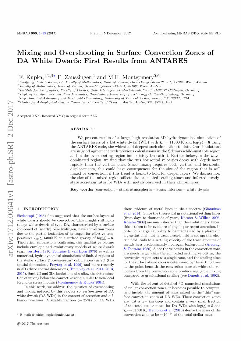
lation, at the beginning of relaxation. For the average overthe last 5scrt of tstat we find Frad(xtop)/Finput to have droppedalready below 1.035, whence Teff ≈ 11900 K. From the timedependence seen in Fig. 5 we expect that a doubling of sim-ulation time from tscrt = 30 onwards, i.e., up to tscrt ≈ 154,would allow halving the residual flux difference to less than2% and thus Teff . 11850 K, in agreement with the relaxationestimate discussed above for tKH (see Fig. 4). We note thatfrom an observer’s point of view we might use the emittedsurface flux, i.e. a Teff of 11912 K, to characterize the simu-lation when averaging it from a tscrt of 70 to 92. However, forthe present discussion we prefer to use the input flux at thebottom (equivalent to Teff = 11800 K) for scaling the results,since this value is fixed throughout the simulation.

The differences between surface and input radiative fluxwhich are expected to remain at that value of tscrt are par-tially caused by the initial stratification of the lower regionnot being in perfect thermal equilibrium, in particular withrespect to its interaction with layers further above. But thereare also systematic differences introduced by numerical in-accuracies of the radiative transfer solver (cf. the little in dipin Ftotal around a depth of 1 km in Fig. 3 — we point out herethat this quantity is not often shown in publications on nu-merical simulations of stellar surface convection, but whenit is, similar features are found for layers near the stellarsurface). Other sources of systematic differences of similarorder or smaller occur when comparing grey with non-greyradiative transfer (cf. Grimm-Strele et al. 2015a and alsoTremblay et al. 2011), or they originate from the detailedimplementation of the input boundary condition as well asfrom differences between the numerical approximation andassumed microphysics of the 1D starting model in compar-ison with the numerical simulation. Although one could tryto “remove” residual flux differences originating from thesesources by longer relaxation, it makes neither physical normathematical sense to do so: the systematic and numericalerrors they contribute to are already roughly equal to theflux difference caused by an “incomplete relaxation” of theorder of 2% of the total flux. For the same reason it is alsonot important whether we estimate tKH(x) by averaging overtstat, as we have done, or calculate it from the initial conditionto guide the simulation. An estimate of the numerical errorsdue to resolution on the mean temperature profile as ob-tained from numerical simulations of solar granulation withANTARES has been made by Grimm-Strele et al. (2015b):the accumulated error over several sound crossing times —for a relative resolution roughly comparable to the one usedin the present work — was found in the range of a fraction ofone percent, with maximum errors up to a few percent. Theerror calculated that way is chiefly due to finite resolution inthe numerical simulation and since the relative resolutions,maximum Mach numbers, etc., are roughly comparable toour present case, we should expect relative (numerical) er-rors of similar size also for the present simulation. Moreover,from Fig. 5 we can see the impact of oscillations present inthe simulations: they lead to a variation in Frad(xtop)/Finputof ±0.5% over τscrt (we discuss those further below).

It is thus of little practical use to extend the presentsimulation over a longer interval in time. If at all, one mayconsider tscrt → 150, since beyond this value the systematicerrors become dominant. But as we show here, also for suf-ficiently accurate statistics of the velocity field time integra-

0.01

0.1

1

0 1 2 3 4 5 6 7 8

rms

velo

city

in [k

m s

-1]

vertical depth in [km] from top of model

DA white dwarf, Finput for Teff=11800 K, log(g)=8

urms, tscrt: [30,40]urms, tscrt: [30,50]urms, tscrt: [40,60]urms, tscrt: [50,70]urms, tscrt: [60,80]urms, tscrt: [70,92]

Figure 6. Relaxation of the root mean square average of the

fluctuation of the u-component of horizontal velocity around its

horizontal mean, urms, displayed as a function of depth and timeaveraged over a sequence of intervals distinguished by model age

tscrt.

tion beyond tscrt ≈ 92 is not necessary. Fig. 6 provides an ex-ample for the rapid convergence of the velocity field towardsa statistically stationary state well within our estimate oftconv(x2) discussed along Fig. 4. We find halving of the rela-tive error of the horizontally and time averaged root meansquare of the fluctuation of the u-component of horizontalvelocity, urms, relative to its instantaneous horizontal meanfor each consecutive interval of 10 scrt, i.e., ∝ tscrt

−2. As canbe estimated from the mere 12% increase through most ofthe layers of the simulation when progressing from a tscrt inthe interval [60,80] to [70,92], i.e. the range of tstat, quadraticconvergence is found for nearly the entire simulation du-ration of tscrt. This is fast enough such that the differencebetween these two averagings is already the entire expectedgrowth if the computation were continued beyond a tscrt ofabout 150. Fig. 6 thus also provides an error estimate forurms with respect to its relaxation.

For the surface layers this error is even much smallerand clearly it converges rapidly throughout the entire sim-ulation box. This similarly holds for the siblings of urms,i.e., vrms and wrms, which characterise the second horizontaland the vertical component of the flow. Also skewness andkurtosis of velocity and temperature fields, i.e., higher-orderstatistical correlations that we discuss below in Sect. 4.2,converge fast but for a limited region dominated by singleevents which is explained there in more detail. We can hencesafely use velocity and temperature statistics averaged overtscrt in the following discussion. From a physical point ofview this fast convergence of the statistics for the velocityfield irrespectively of the less accurate convergence of theemerging radiative flux is not surprising: the velocity fieldsare generated by convective processes occurring in the up-per part of the simulation box (with very short relaxationtimes). All what is left is a small drift as a function of time,which does not affect the functional form, physical processes,and even the level of accuracy we expect from the velocityrelated quantities that we discuss below. The independenceof the residual error in the velocity field from the degree of

MNRAS 000, 1–13 (2017)

6 F. Kupka et al.

0.01

0.1

1

10

0 1 2 3 4 5 6 7 8

rms

velo

city

in [k

m s

-1] a

nd a

niso

tropy

ratio

vertical depth in [km] from top of model

DA white dwarf, Finput for Teff=11800 K, log(g)=8

wrmsurmsvrms

Φ=<u2+v2+w2>/<w2>linear fit of Φ in [4.45,5.85]

Figure 7. Vertical rms velocity, wrms, and its horizontal counter-

parts, urms and vrms, perfectly agreeing, on a logarithmic scale. Thedimensionless anisotropy ratio Φ is also plotted together with its

linear fit computed for the interval from 4.45 km to 5.85 km.

thermal relaxation is also corroborated by the completelydifferent convergence rates, ∝ tscrt

−2 for urms and ∝ tscrt−1/2

for the total (radiative) flux at the surface. We expect thefaster convergence rate of velocities to change to the smallerone of thermal relaxation once tscrt & tconv(x2)/τscrt ≈ 127. Asdiscussed in the context of thermal relaxation, at this pointin time evolution the model intrinsic errors dominate overthe residual error, and the accuracy reached for urms and re-lated quantities at tscrt ∈ [70,92] is already adequately small.Thus, our simulation data obtained over tstat are both basedon a sufficiently well relaxed simulation and have statisticalerrors small enough to be useful subsequently.

3.3 Velocities

As the vertical and horizontal velocity fields are reasonablywell converged in the convection zone and in the overshoot-ing region underneath, we can analyse the time and horizon-tally averaged root mean square of their fluctuating compo-nents, i.e., wrms for the vertical velocity, and likewise urmsand vrms for the two horizontal components. In Fig. 7 weplot them on a logarithmic scale. From local maxima of∼ 5.7 kms−1 near the top of the convective zone they gradu-ally drop towards its bottom. Where Fconv changes sign (seeFig. 3), urms and vrms have reached ∼ 1.8 kms−1 while wrmsis still ∼ 2.8 kms−1, but has begun to decay much faster, aprocess occurring for urms and vrms again from around 3.2 kmonwards. The horizontal velocity components begin to domi-nate the total kinetic energy and Φ = (w2

rms +u2rms +v2

rms)/w2rms

exceeds a value of 2 with a local maximum around 3.5 km.There, a rapid, exponential decay sets in. It is slightly largerfor urms and vrms. For wrms the decay slows down around 4 km,where Fconv begins to vanish (−1% . Fconv/Finput . 0%). Thedecay of urms and vrms continues to be rapid down to about4.2 km and Φ < 2. The simulation can be used for an accu-rate study of even deeper layers where the lower boundaryis still sufficiently away to avoid direct interference. We findthat velocities decay at a slower rate than in the “overshoot-ing zone proper”. Interestingly, urms and vrms continue to de-

-8

-7

-6

-5

-4

-3

-2

-1

0

1

2

-2 -1 0 1 2 3 4

ln v

z,rm

s, ln

wrm

s

ln P

DA white dwarf, Finput for Teff=11800 K, log(g)=8

ln wrms ln urms ln vrms

exponential decay with Hp

Figure 8. Logarithm of wrms, urms, and vrms, as functions of thelogarithm of total pressure, relative to a reference velocity and

pressure. The exponential decay hypothesis for wrms as function

of pressure scale height is indicated.

0

1

2

3

4

5

6

7

8

9

10

3.8 4 4.2 4.4 4.6 4.8 5 5.2

rms

velo

city

in [k

m s

-1]

horizontally averaged log(T) of model, [T] in K

DA white dwarf, Finput for Teff=11800 K, log(g)=8

wrmsurmsvrms

Φ=<u2+v2+w2>/<w2>linear fit of wrms in [4.68:4.78]

Figure 9. Φ as well as wrms, urms, and vrms as functions of logTalongside a linear fit of wrms in the overshooting region (see text).

cay more rapidly than wrms: over an extended region fromabout 4.45 km to 5.85 km Φ features a nearly linear decreasewith depth which ceases only once the influence of the lower(closed) boundary condition becomes notable. Fig. 7 high-lights this relation by a linear least squares fit of Φ for thatregion. Note that the logarithmic scale in that figure wouldactually suggest an exponential fit for Φ while a plot in lin-ear scale motivates the linear model function chosen. Thissmall difference is caused by a very low e-folding scale: in thiscase an actually exponential function can be approximatedby a linear function over an extended range. We return to acomparison between both models in Sect. 4.3.2.

In Fig. 8 we plot the logarithm of wrms as well as urmsand vrms as functions of ln P, normalised relative to the ve-locity and the total pressure at the layer where Fconv changessign (at 2.785 km in Fig. 3). We also plot a line to indicatean exponential decay of the vertical velocity field with Hp,as proposed in Tremblay et al. (2015) to occur for DA WDs.We cannot identify a unique exponential scaling law for wrms

MNRAS 000, 1–13 (2017)

Mixing and overshooting in DA white dwarfs 7

in regions where Fconv < 0. For the layers where ∆ lnP is be-tween 0 and 1.5 (|Fconv/Finput| > 1%), the decay rate is firstabout 1Hp, then becomes twice as steep (0.5Hp), then settlesat a quarter of that rate (2Hp). Similar holds for urms andvrms with a shift in location and different decay rates partic-ularly for ∆ lnP& 1.5. No simple polynomial law can describethis dependency either (Canuto & Dubovikov 1997 deriveda polynomial decay as function of distance from the convec-tion zone if the dissipation rate of turbulent kinetic energywere computed from its local limit expression, cf. Fig. 7).

In turn, wrms depends linearly on logT from 2.73 km,where Fconv & 0, down to about 3.73 km, where Fconv/Finput ≈−2% (see Fig. 9). The linear fit of wrms as a function of logTfinds wrms to become zero where Fconv/Finput ≈ −0.87%, al-though this occurs below the domain of its validity. There,logT ≈ 4.80 at a depth of ≈ 3.97 km. Inside the fit region,∆ lnP increases from −0.07 to 1.04. A linear decay of wrmsas a function of logT for exactly the same part of the over-shooting region has been reported by Montgomery & Kupka(2004) for hotter DA WDs with Teff & 12200 K when solvingthe Reynolds stress model of Canuto & Dubovikov (1998).Note that the same scaling could also be inferred from Fig. 4of Tremblay et al. (2015) for their models with a Teff of12100 K, 12500 K, and, roughly, also 13000 K for “zone 3”(cf. their Table 1). As hydrogen is fully ionised in that zoneand Ftotal ≈ Frad, both T and Hp scale linearly with depth,thus our Fig. 9 and Fig. 1 of Montgomery & Kupka (2004)imply the same (non-) linear decay of wrms with T and Hp,albeit (cf. Fig. 8) this also only holds for a limited region.

4 ANALYSIS

4.1 The temperature field and overshooting

One may characterise an overshooting zone with respect tothe sign of the convective flux, the superadiabatic gradient(or alternatively the gradients of entropy or potential tem-perature), the flux of (turbulent) kinetic energy, the massflux, or the local maxima and minima of these quantities.Assuming a nearly adiabatic temperature gradient for casesof convection at low radiative loss rates (high Peclet number)Zahn (1991) distinguished a separation of the Schwarzschildunstable convection zone proper (Fconv > 0, ∇ > ∇ad, with|∇−∇ad|/∇ad � 1), from the zone of subadiabatic penetra-tion (Fconv < 0, ∇ < ∇ad, while again |∇−∇ad|/∇ad � 1),and the thermal boundary layer (Fconv < 0, ∇ < ∇ad, but|∇−∇ad|/∇ad→ O(1)), until eventually Fconv ≈ 0 (stable, ra-diative region, no longer mixed by convection). This caseof penetrative convection he distinguished from the case ofovershooting for which a more narrow definition was sug-gested: there, large radiative losses prevent altering the tem-perature gradient towards the adiabatic one in regions whereFconv < 0.

For the DA white dwarf we consider in the present case,it follows from Fig. 3 that radiative losses everywhere inthe overshooting region are large (low Peclet number). So itmakes sense to distinguish, as in Freytag et al. (1996), thefollowing regions. First of all, the convection zone properwith its Schwarzschild boundary (Fconv > 0, ∇ > ∇ad) andthen an overshooting region where plumes gradually heat upthat do not yet experience negative net buoyancy (and which

we call countergradient region, Fconv > 0, ∇ < ∇ad). The layerat which the change of sign in Fconv occurs is termed “fluxboundary” by some authors, for example, in Tremblay et al.(2015). From there onwards throughout where Fconv < 0 and∇ < ∇ad, plumes penetrate into a region of counterbuoyancy.We call this the plume-dominated region in the following.One might also consider the local minimum of Fconv to markthe region where the thermal boundary layer begins, as inZahn (1991), although this has a less important role, as wesee in the following figures. Finally, motion can persist be-yond where Fconv→ 0 and ∇ < ∇ad, which we further belowcall the wave-dominated region. The reasons for this namingbecome evident from the following figures.

In Fig. 10a, well inside the convection zone, the networkof intergranular lanes is still clearly visible, similar to thestellar surface depicted in Fig. 1, although the temperaturecontrast between maximum and minimum values has be-come larger and more skewed (low temperature regions covera smaller area). At the Schwarzschild boundary, Fig. 10b, thegranular structure is still recognizable, but the intergranular“network” of downflows is no longer connected; rather, it ischaracterised by plumes, chiefly grouped together near cor-ner points where several granules meet each other in layersinside the convection zone. The now isolated, cold down-flow columns maintain their identity (Fig. 10c), althoughthey gradually lose the contrast between them and theirenvironment, until the “flux boundary” is reached, whereFconv changes sign (Fig. 10d). Below this level the structurerapidly changes: the temperature contrast is drastically re-duced over a small distance, from 3 : 2 at the flux boundaryaround 2.75 km to just 7 : 6 at 3.00 km (Fig. 10e). Nowthe plumes have reverted their role: they are hotter thantheir environment. This structure is maintained throughoutthe entire plume-dominated region (Fig. 10e–g). The con-trast drops only gently (down to 9 : 8), but more impor-tantly, the number of plumes per area and the area each ofthem covers rapidly decrease. Indeed, at 4.00 km we see justone strong plume left in comparison with some three dozenat 3.00 km. As we know through Fig. 3, around 4.00 km,Fconv/Ftotal→ 0 (essentially), and a new pattern becomes vis-ible. This pattern remains throughout the wave-dominatedregion depicted in Fig. 10h–i, with the small contrast be-tween maximum and minimum temperature slowly decreas-ing from 2.2% to 1.5%. This continues further into the wave–dominated region (e.g., to a contrast of 1.2% at 5.50 km, notshown in Fig. 10), although the visible structures have nolonger the trivial vertical correlation which is easily found forthe layers further above. We remark here that the flow pat-terns — which allow an easy distinction between the convec-tively unstable, the counter–gradient, the plume–dominatedand the wave–dominated region — are present already attscrt = 35. They are not related to the patterns of initial relax-ation, say at tscrt = 30.1, where the wave–dominated region isstill mostly unperturbed (∆T < 1K at 5.00 km) and the pat-tern visible in the plume–dominated region has very little,if any, relation to what can be seen in the wave–dominatedregion 5 scrt later. We conclude that the patterns observedin Fig. 10 are intrinsic to the flow, but not to the initial per-turbation chosen to start it, either in the wave–dominatedregion, or in any layer further above. We skip a similarlydetailed discussion of the velocity field and instead demon-strate how skewness and kurtosis capture many of the sta-

MNRAS 000, 1–13 (2017)

8 F. Kupka et al.

Figure 10. Horizontal cuts of temperature as a function of depth at time tscrt = 92. The top row displays snapshots at depths of 1.50 km,

2.00 km and 2.50 km (Fig. 10a–c) as measured from the top of the simulation box. The middle row continues this series for depths of2.75 km, 3.00 km and 3.50 km (Fig. 10d–f). The bottom row displays the cuts for depths of 4.00 km, 4.50 km and 5.00 km (Fig. 10g–i). Note that the temperature scale changes for each snapshot and the ratio between maximum and minimum value peaks near theSchwarzschild stability boundary around 2.00 km. Clearly inside the plume-dominated region it is already smaller and drops only gently

from 3.00 km to 4.00 km. There is again a drastic drop in scale for layers inside the wave-dominated region.

tistical and topological properties of the velocity and tem-perature field.

4.2 Skewness and kurtosis of velocity fields andtemperature

In Fig. 11 we display the skewness of fluctuations of thetemperature field, Sθ , and the vertical (w) and horizontal

components of the velocity field, Sw, Su, and Sv, aroundtheir horizontal mean, averaged over each layer and intime (over tstat), plotted as a function of depth. The neg-ative values of Sθ = 〈(T − 〈T 〉h)3〉h,t/(〈(T − 〈T 〉h)2〉h,t)3/2 =

〈T ′3〉h,t/(〈T ′2〉h,t)3/2 within the convectively unstable zone in-dicate that locally low values of T cover a smaller surfacearea and hence have to deviate further from the horizon-tal mean value than locally high values, in perfect agree-

MNRAS 000, 1–13 (2017)

Mixing and overshooting in DA white dwarfs 9

-5

-4

-3

-2

-1

0

1

2

3

0 1 2 3 4 5 6 7 8

skew

ness

vertical depth in [km] from top of model

DA white dwarf, Finput for Teff=11800 K, log(g)=8

SwSuSvSθ

Figure 11. Skewness of fluctuations of the temperature field, Sθ ,and the components of the velocity field, Sw,Su,Sv, around their

horizontal mean, averaged over each layer and in time (over tstat),plotted as a function of depth.

ment with Fig. 10a. Within the countergradient region thisbecomes even more pronounced due to the fast columns ofdownflows generated by the strongest remnants of the down-flow network (cf. Fig. 10c). The situation becomes reversedaround the flux boundary (Fig. 10d) and the plumes, whichcover a smaller area than the upflow, are now hotter thantheir environment (Fig. 10e–f). Hence, Sθ > 0 in that re-gion with a pronounced global maximum where Sw has itsglobal minimum. Eventually, in the wave-dominated region,Sθ → 0 which demonstrates that the temperature distribu-tion is symmetric around its horizontal mean in those layers.In comparison, Sw, which is defined analogously to Sθ , but forthe vertical velocity field, also demonstrates that the down-flows cover a more narrow area than the upflows (due toconservation of mass and momentum), whence Sw < 0 in theconvection zone. The distribution becomes more and moreskewed once the network of downflows has transformed intoa set of plumes where only the fastest and hottest one canpenetrate sufficiently deep (cf. Fig. 10f and note its locationclose to the global extrema of Sw and Sθ ). Once the plumesdisappear in number, Sw→ 0 and remains near that value forthe entire wave-dominated region. Since the simulation has(or, rather, should have) no preferred symmetry of velocitiesinto any of the horizontal directions, we expect Su ≈ 0 andSv≈ 0 throughout the simulation and this is also an indicatorfor the degree of convergence of the statistical results. Wefind this confirmed by Fig. 11 with one exception: around4 km, both Su and Sv deviate from 0 and this can be un-derstood as resulting from the statistics depending on veryfew events with large impact, i.e., on a few plumes manag-ing to penetrate deep enough (Fig. 10g), leading eventuallyto sidewards flow by conservation of mass. Many more suchevents are required to obtain a converged statistical resultwithin tstat in that region at the given horizontal extent ofour simulation.

In Fig. 12 we display the kurtosis of fluctuations ofthe temperature field, Kθ , and the vertical and horizon-tal components of the velocity field, Kw, Ku, and Kv, com-puted in analogy to skewness except that now Kθ = 〈(T −

0

20

40

60

80

100

120

0 1 2 3 4 5 6 7 8

kurto

sis

vertical depth in [km] from top of model

DA white dwarf, Finput for Teff=11800 K, log(g)=8

KwKuKvKθ

Figure 12. Kurtosis of fluctuations of the temperature field, Kθ ,and the components of the velocity field, Kw,Ku,Kv, around their

horizontal mean, averaged over each layer and in time (over tstat),

plotted as a function of depth (full range of kurtosis shown).

1

2

3

4

5

6

7

8

9

10

0 1 2 3 4 5 6 7 8

kurto

sis

vertical depth in [km] from top of model

DA white dwarf, Finput for Teff=11800 K, log(g)=8

KwKuKvKθ

Figure 13. Kurtosis of fluctuations of the temperature field, Kθ ,

and the components of the velocity field, Kw,Ku,Kv, around theirhorizontal mean, averaged over each layer and in time (over tstat),

plotted as a function of depth (values truncated above 10).

〈T 〉h)4〉h,t/(〈(T − 〈T 〉h)2〉h,t)2 = 〈T ′4〉h,t/(〈T ′2〉h,t)2, and like-wise for the components of the velocity field. The kurtosisprovides a measure of the strength and importance of devia-tions of a fluctuation from a given root mean square average.For a mathematically meaningful distribution, K > 1. For aGaussian distribution, K = 3 in addition to S = 0. These arenecessary though not sufficient conditions for Gaussianity.As one can read from Fig. 12 the plumes lead to extremevalues of Kw, especially where a few, isolated plumes domi-nate the distribution (around 4 km). In comparison, for Kθ

the flux boundary with its reversion from cold to hot plumesleads to a local minimum in that region (around 3 km). Forthe Sun or other main sequence stars (Kupka & Robinson2007; Kupka 2009) the network of downflows with its embed-ded granules leads to global minima of Kθ and Kw at the su-peradiabatic peak and we find this also for our simulation ofa DA white dwarf (neglecting the top of the simulation box)

MNRAS 000, 1–13 (2017)

10 F. Kupka et al.

(see Fig. 13). Likewise, for both Kθ and Kw the plumes inthe overshooting region lead to very large values of K whichcharacterises their large deviation from the root mean squarevalues of fluctuations of vertical velocity and temperature.In the wave-dominated region eventually K→ 3 for each ofthe four fields depicted in Fig. 13. Along with their values ofS≈ 0 this demonstrates their different nature in comparisonwith the plume-dominated region further above. We notethat the plumes also lead to very large values of Ku and Kvsince they lead to locally very large velocities (the precisevalues at Fig. 12 around 4 km are less certain again due tothe limited statistics of a small number of plumes).

4.3 Properties of the velocity field and mixing

4.3.1 Analysis of the velocity field and best fit functions

With the statistical and topological properties of the veloc-ity and temperature field in mind we now turn to a moredetailed characterization of overshooting and its associatedroot mean square velocity fields.

We find an exponential decay of wrms only in a verygeneral sense. As we have shown in Sect. 3.3, in the plume–dominated region down to the deepest layer where stillFconv/Finput < −1%, the assumption of a linear dependenceof wrms on logT allows an accurate fit. Indeed, its root meansquare deviation normalised to the data range is just . 1.2%over a range of ∼ 1.1Hp (Fig. 9). If the fit is made with Tas an independent variable over the same depth region, oneeven obtains a marginally lower fit error (by 0.07%). Thesmallness of the difference between the two is due to thelimited region in logT over which the fit occurs. We expectthat from the viewpoint of a physical interpretation, the lin-ear fit in T is physically more relevant. Now if we insteadaim at finding the best exponential fit of the velocity fieldwhich at least partially includes the plume–dominated re-gion and is of identical extent (∼ 1.1Hp), we have to shiftthe ∆ lnP range (see Fig. 8) to the region from 0.35 to 1.45to obtain a root mean square deviation normalised to datarange of . 1.6% for ∆ lnwrms. This is larger by 1/3 comparedto the linear fit in T . Moreover, as discussed in Sect. 3.3, thefit in logT (or T ) occurs over exactly the plume–dominatedregion, except for the lowermost part, which is dominated byrare events (single plumes) and even for this region the fit ofwrms versus logT is at least good for deriving a lower limit forthe region which can be assumed to be very well mixed byovershooting (down to ∼ 4 km or log(1−Mr/M?) ∼ −13.9).In comparison, the clearly poorer exponential fit begins onlyaround 3.08 km and ends around 4.14 km. Thus, it starts al-ready right inside the plume-dominated region and includesthe physically very different region where plumes have es-sentially disappeared. It is hence both less accurate and hasa less obvious physical motivation.

As mentioned already in the discussion of Fig. 8 inSect. 3.3, one could attempt fitting also the transition re-gions from the plume–dominated to the counter–gradient re-gion and from the plume–dominated to the wave–dominatedregion by exponential fits with different decays. However,these hold for even smaller depth ranges and we see lit-tle physical motivation for them beyond providing decentmathematical fits. A “compromise exponential fit” for both

transition regions and the plume–dominated region yields aclearly poorer result than any of the more localised fits.

We hence suggest that the best approximation for theplume–dominated region is that of an approximately lineardecay of rms velocities with depth, as it is also found fromthe Reynolds stress model as used by Montgomery & Kupka(2004). We emphasise that this statement is restricted tothe case of overshooting zones with strong, hot plumes thatare subject to high radiative losses. Clearly, this does notinclude the case where convection zones have a marginalFconv/Finput already inside the convective zone itself (i.e., forTeff & 13000 K) and to understand the complex variation ofovershooting with parameters such as Teff and log(g), whichwas studied by Tremblay et al. (2015), requires a grid ofmodels, as has indeed been used by these authors.

4.3.2 The wave–dominated region

How is the region underneath the plume–dominated regiondifferent from layers further above it? In previous literatureon overshooting inside stars, little attention appears to havebeen paid to the horizontal velocity field. As Fig. 7 demon-strates, after a transition region of ∼ 0.5 km below the verywell mixed region, we find a nearly linear decay of horizontalkinetic energy relative to vertical one (see the behaviour ofΦ in Fig. 9 and Fig. 7). This is remarkable, since horizontalvelocities are expected to increase relative to vertical ones,if the flow approaches a closed, stress-free vertical boundary.Φ decreases linearly over 1.15 pressure scale heights with anerror of . 1.9%. We note that an exponential decay at op-timised decay rate is slightly better (. 1.4%). If optimisedfits of exponential decay are individually made for wrms, urms,and vrms, residual errors are in the range of 0.5%–0.9%. Thus,although the decay of the root mean square velocity fieldsand the quantity Φ is exponential to very high accuracy,we can use the linear decay of Φ observed in the simulatedregion as a lower estimate for the extent of mixing.

We emphasise that the clear identification of this expo-nential decay for the case of overshooting with strong, hotplumes (i.e., at the Teff of our simulation target) requiresthe extra extent of ∼ 1Hp in comparison with earlier work(Tremblay et al. 2011, 2013, 2015 and even more so Freytaget al. 1996). This allows a clear separation of the impact ofthe lower boundary condition on the velocity fields, espe-cially on the horizontal components, where this is more pro-nounced (Fig. 7). The detailed analyses of exponential decayof velocities underneath the convection zone have focussedmore on hotter DA white dwarfs in earlier work, for whichconveniently a sufficiently deep simulation is more easilyachieved, because the equivalence of a plume-dominated re-gion cannot exist in their case, as |Fconv|/Finput . 1% for thesestars even inside their convectively unstable zone. Thus, thetotal number of pressure scale heights needed in a simula-tion to model the wave-dominated region such that at leastthe upper part of it is not affected by the lower boundarycondition is smaller.

Since in our case, only underneath about 6 km, at stilla pressure scale height distance from the lower boundarycondition, the latter begins to notably influence the flow, weconclude the decay of horizontal relative to vertical veloci-ties, which is visible in each of Fig. 7–9, to be real. Belowabout 4 km (where Frad→ Ftotal), the flow gradually changes

MNRAS 000, 1–13 (2017)

Mixing and overshooting in DA white dwarfs 11

16 17 18 19 20 21 22

time (sec)

�1.0

�0.5

0.0

0.5

1.0

�Fra

d/�T

4 e↵

(%)

Antaresfit (P=0.263 s)

0 2 4 6 8 10 12 14

Frequency (hz)

0.00

0.05

0.10

0.15

0.20

0.25

0.30

0.35

Am

plitu

de

(%)

Figure 14. Pressure oscillation mode in our numerical simula-tion, whose period is close to the sound crossing time. In the

upper panel we show the fractional variation of the radiative flux

emerging at the top of the simulation domain after division bya polynomial fit to remove the trend due to thermal relaxation

(blue, solid curve); the dotted (red) curve shows the sinusoidal fit

to these data. The lower panel gives the Fourier transform of thenormalized flux variations, which indicates a mode with a period

of 0.263 s and an amplitude of ∼ 0.3%.

into a slow, chiefly vertical, and thus a more wave-like mo-tion. Independently from the limitations of even the presentsimulation, it is clear that a lack of horizontal flow preventsmixing. Thus, the mixing in this region is much less efficientthan in the layers of notable convective energy flux, and theeffective diffusivities and mixing time scales are expected todiffer by a very large amount, since a wave-like motion ismuch less efficient in entraining fluid in comparison to anoverturning flow.

In the region between 4.45 km and 5.85 km the fluctua-tions of density and temperature decay rapidly (. 3 ·10−3 oftheir horizontal mean). Skewness and kurtosis, as depictedin Fig. 11–13 of the velocity and temperature fluctuations,yield S = 0±0.06 and K = 3±0.2 for all layers below 4.85 km(at 3.5 km we find K� 3, |S|> 1). This excludes a flow witha granulation pattern or thin plumes embedded in gentlymoving upflows, as is proven by Fig. 10. The componentsand magnitude of vorticity of u drop faster than wrms, urms,and vrms in that region. No indications for “extreme events”have appeared during tstat.

We also observe a stable oscillation, a vertical, globalpressure mode without interior node, which is easily vis-ible for the horizontally averaged, vertical mean velocity.It has a frequency of νosc = 3.7959Hz and thus a period ofPosc = 0.26344s. Its amplitude is ∼ 30 ms−1 at ∼ 5.85 kmwhere wrms∼ 105 ms−1. It can also be identified in the emerg-ing radiative flux even though in this case it is subject to per-turbations by local events (shock fronts, etc.) and drift dueto thermal relaxation (discussed in the context of Fig. 5). Af-

ter removing the latter from Frad(x = 0km, t) by a polynomialfit, it is easy to extract the dominant mode frequency, as isdemonstrated in Fig. 14. Once excited, this oscillation can-not be removed from the simulation by artificial damping,if that were attempted (we have done a number of experi-ments with 2D simulations to corroborate that), so evidentlythe convection zone in the simulation is able to feed themode energetically at a sufficiently high rate against damp-ing mechanisms (due to radiative losses, viscosity, etc.) tosupport this very stable amplitude. The mode is also presentthroughout the convection zone and even has its maximumamplitude right there where it provides just a small fractionof the kinetic energy of the flow.

The oscillation with a frequency of νosc can also be iden-tified when tracing hot or cold structures in Fig. 10h–i, inwrms, or in Frad (see Fig. 5). Thus, the flow taking place inthe region below 4 km is a combination of global waves andlocal, transient features. Its properties with respect to skew-ness, kurtosis, vorticity, the clear presence of a global verticalmode with a significant contribution (∼ 10%) to the kineticenergy in that region, and the decrease of Φ (and thus thefaster decrease of horizontal in comparison with vertical ve-locities) justifies its naming as wave–dominated region. Butthese properties are at variance with efficient mixing andwe thus expect the mixing processes in the two regions, theovershooting zone proper and the wave–dominated region,to differ physically and in their efficiency.

Now one might use the velocity field found in the nu-merical simulation, as has been done before (Freytag et al.1996, Tremblay et al. 2015, e.g.), and derive a depth be-low which diffusion velocities dominate and in this sensedefine an extent of the mixed region. We have to point outhere a major caveat of this procedure: just as simulationsof solar surface convection, which have open lower verticalboundaries, the solid, slip boundaries used for simulationswith a radiative region at the bottom also reflect verticalwaves. Thus, while fluid can leave or enter the domain onlyin the former case, both types of boundary conditions con-serve momentum inside the box and create a reflecting layerfor vertical waves at the bottom of the simulation box. Forboth cases waves in a real star should have smaller maxi-mum amplitudes due to the simple fact that the mode masscontained in the simulation box is much smaller. Ampli-tudes of p-mode oscillations hence have to be scaled by modemass (Stein & Nordlund 2001) to be compared to observa-tions (or models of the entire star). Although the theoreticalexplanation of waves excited in the overshooting zone pro-posed by Freytag et al. (1996) is based on g−-modes ratherthan p-modes, we expect the former also to be altered (to-wards exhibiting a much lower equilibrium amplitude) dueto the fact that in a real star such waves connect to a muchlarger mass. Hence, we expect that the velocities obtainedfor the wave–dominated region are systematically overesti-mated compared to a model of a full star. A determinationof the mixed region by means of wrms then leads to an evenmore pronounced overestimation. Consequently, as an upperlimit of the mixed region one should rather use urms and vrmsor an exponential fit of Φ.

Having the inevitable overestimations by this procedurein mind and without a suitable method of scaling of the ve-locity fields yet at hands, we may also consider the linear fitof Φ which at least provides a lower estimate for mixing due

MNRAS 000, 1–13 (2017)

12 F. Kupka et al.

to the processes in the wave–dominated region, if the veloci-ties of the numerical simulation in that part are taken at facevalue. Indeed, if we extrapolate the linear fit of Φ, it wouldreach a value of 1 at ∼ 7.67 km, some 5.67 km below thelower boundary of where ∇ > ∇ad still holds. This hopefullyprovides a safe, lower limit for the extent of the well mixedregion; it corresponds to a mass of log(1−Mr/M?) ∼ −12.7in our stellar model.

4.3.3 Mixing and accretion

For the case of steady-state accretion of metals, the ob-served surface abundance results from a competition be-tween the accretion rate onto the surface and the settlingrate of the metals at the base of the mixed region. Using thepublished values of Koester (2009, Tables 1 and 4), we canestimate the effect that mixing beneath the formally con-vective region has on the settling rates for trace amountsof metals in a hydrogen atmosphere white dwarf. If we as-sume that mixing only occurs in the region defined by theSchwarzschild criterion, the base of the mixed region wouldbe at log(1−Mr/M?)∼−15.2; interpolating in Tables 1 and 4of Koester yields a settling time for carbon of τ−15.2∼ 0.14yr.On the other hand, if we assume the base of the mixed regionis at log(1−Mr/M?)∼−13.9, corresponding to the depth ofpenetration of the plumes, then we find the settling time ofcarbon is τ−13.9 ∼ 1.4yr. Finally, if we take the base of themixed region to be log(1−Mr/M?) ∼ −12.7 (where Φ = 1 isextrapolated from the ANTARES simulation), then we ob-tain a settling time for carbon of τ−12.7 ∼ 12yr. The ratioof this settling time to that assuming mixing only in theSchwarzschild unstable region is ∼ 87. For the elements Na,Mg, Si, Ca, and Fe, we find similar ratios for the enhance-ment of their settling times, in the range of 50–97. Thus,including the mixing in the overshooting region has a verylarge effect on the computed settling times of metals in WDenvelopes.

In a similar vein, we would like to examine the ef-fect that a larger mixed region has on the inferred accre-tion rates, assuming steady-state accretion. From Eq. 6 ofKoester (2009), XCZ = τCZMX (MCZ)−1, where XCZ is the massfraction of element X in the convection zone, τCZ is the set-tling time at the base of the mixed region, MX is the massaccretion rate of element X , and MCZ is the mass of themixed region. If we assume that XCZ is fixed by the obser-vations, then MX ∝ MCZ/τCZ. Using log(1−Mr/M?) ∼ −15.2and −13.9 for the extent of the mixed region with and with-out overshooting, respectively, we find that including theovershooting region enhances the inferred accretion rates byfactors of 1.6–2.5 for the set of metals previously considered.If instead we take the depth of the overshooting region tobe at log(1−Mr/M?)∼−12.7, then we find that the inferredaccretion rates are enhanced by factors 3.2–6.3 for the sameset of metals with respect to the no-overshooting case.

We point out here that the total mixed mass obtainedfrom the linear fit of Φ with the requirement Φ → 1 isroughly 300 times larger than that contained in and abovethe Schwarzschild-unstable region. This number is similarto suggestions by Freytag et al. (1996), Koester (2009), andwithin the (much larger) range suggested by Tremblay et al.(2015).

5 DISCUSSION AND OUTLOOK

We have highlighted here that estimates for the extent ofthe mixed region underneath the surface convection zoneof DA white dwarfs at intermediate effective temperatures(Teff ≈ 11800 K) as obtained from (3D) hydrodynamical sim-ulations have to be revisited from a new perspective. Thishas become possible thanks to the larger (3D) simulationdomain and the simulation being performed over a sufficientamount in time. The larger horizontal extent reduces arti-facts by the periodic boundary conditions and allows a bet-ter sampling of statistical data due to a larger number of re-alizations. The larger vertical extent allows for the first timea clear identification of exponential decay of the velocityfield, as a function of depth, underneath a region dominatedby plumes. In the latter, exponential fits lack both accuracy,since the decay rate itself would have to be a function ofdepth, and also a physical basis, since the upper parts of theovershooting zone are completely dominated by plumes andtheir dynamics instead of waves (even though the latter areof course also present in that part of the simulation domain).In the plume–dominated region (once Fconv < 0) we find a lin-ear decay with depth to provide a more accurate model andin this sense the simulations agree qualitatively and, roughly,quantitatively with solutions of Reynolds stress models forsomewhat hotter objects (cf. Montgomery & Kupka 2004).The wave–dominated region, for which we confirm exponen-tial decay of the vertical root mean square velocity, is notmodelled by the Reynolds stress approach (as the time de-pendent mean velocity was assumed to be zero, so it can-not be included in the model used by Montgomery & Kupka2004). Viewing our results at a more coarse level we also con-firm some basic findings of earlier studies (especially fromFreytag et al. 1996 and Tremblay et al. 2011, 2013, 2015)performed with different simulation codes and with smallerdomain sizes.

Contrary to earlier work we stress here that the hori-zontal velocities, which decay more rapidly than the verticalones in the wave–dominated region, provide an indicationfor a less efficient mixing. We also point out that the ampli-tudes due to waves obtained from this class of simulationsshould be expected to be systematically too large. Thus,while the convective mixing due to overshooting up to andincluding the plume–dominated region is on safe ground, itsextension into the wave–dominated region is much less cer-tain and certainly subject to gross overestimation. We thusprovide a linear extrapolation based on horizontal velocitieswhich might be used as a more conservative estimate of theextent of the convectively mixed region.

We emphasise here that our results have been obtainedfor the case of a DA white dwarf with a large amount of con-vective flux inside the unstable zone which features strong,long-lived plumes penetrating into the stably-stratified re-gion. Further studies should clarify the dependencies of theseresults on Teff and log(g), and, with respect to the wave-dominated region, on simulation depth and time.

Finally, we show that the extent of the mixed regioncan have a large effect on the computed settling times andaccretion rates of metals in WDs also when using our moreconservative estimates of the extent of mixing due to over-shooting. While we think there is merit in the prescriptionwe have adopted for defining the extent of the mixing region,

MNRAS 000, 1–13 (2017)

Mixing and overshooting in DA white dwarfs 13

it is probably a lower limit compared to results which assumemixing velocities to decrease exponentially with depth. Moreprecise estimates of this kind clearly require further work,not only from the viewpoint of simulations, but also withrespect to some theoretical aspects such as mixing efficiencyof the encountered types of flows and characterizations ofthe effect of limited simulation domain sizes.

ACKNOWLEDGEMENTS

F. Kupka gratefully acknowledges support through AustrianScience Fund (FWF) projects P25229 and P29172. Parallelsimulations have been performed at the Northern GermanNetwork for High-Performance Computing (project numberbbi00008) and the Heraklit cluster at the BTU Cottbus-Senftenberg. M. H. Montgomery gratefully acknowledgessupport from the United States Department of Energy undergrant DE-SC0010623 and the National Science Foundationunder grant AST-1312983.

REFERENCES

Arcoragi J. P., Fontaine G., 1980, ApJ, 242, 1208

Bohm K. H., Cassinelli J., 1971, A&A, 12, 21

Canuto V. M., Dubovikov M., 1997, Astrophys. Jour., 484, L161

Canuto V. M., Dubovikov M., 1998, Astrophys. Jour., 493, 834

Dupuis J., Fontaine G., Pelletier C., Wesemael F., 1992, ApJS,

82, 505

Fontaine G., van Horn H. M., 1976, ApJS, 31, 467

Freytag B., Ludwig H.-G., Steffen M., 1996, Astron. Astrophys.,313, 497

Gianninas A., Dufour P., Kilic M., Brown W. R., Bergeron P.,

Hermes J. J., 2014, ApJ, 794, 35

Grimm-Strele H., Kupka F., Low-Baselli B., Mundprecht E.,Zaussinger F., Schiansky P., 2015a, New Astron., 34, 278

Grimm-Strele H., Kupka F., Muthsam H., 2015b, Comp. Phys.

Comm., 188, 7

Happenhofer N., Grimm-Strele H., F. K., Low-Baselli B., Muth-sam B., 2013, Journal of Computational Physics, 236, 96

Herwig F., 2000, Astron. Astrophys., 360, 952

Iglesias C., Rogers F., 1996, Astrophys. Jour., 464, 943

Kippenhahn R., Weigert A., 1994, Stellar Structure and Evo-

lution, 3rd corr. edn. Astronomy and Astrophysics Library,Springer, Berlin; New York

Koester D., 2009, A&A, 498, 517

Koester D., Wilken D., 2006, A&A, 453, 1051

Kupka F., 2009, Mem. della Soc. Astron. Ital., 80, 701

Kupka F., Muthsam H., 2017, Living Rev. in Comp. Astrophys.,3:1, 159 pp.

Kupka F., Robinson F. J., 2007, Mon. Not. R. Astron. Soc., 374,305

Kupka F., Ballot J., Muthsam H. J., 2009, Communications inAsteroseismology, 160, 30

Montgomery M. H., Kupka F., 2004, Mon. Not. Roy. Astron. Soc.,

350, 267

Mundprecht E., Muthsam H. J., Kupka F., 2013, Monthly Noticesof the Royal Astronomical Society, 435, 3191

Muthsam H., Kupka F., Low-Baselli B., Obertscheider C., Langer

M., Lenz P., 2010, New Astron., 15, 460

Paczynski B., 1969, Acta Astron., 19, 1

Paczynski B., 1970, Acta Astron., 20, 47

Pamyatnykh A. A., 1999, Acta Astronomica, 49, 119

Rogers F., Swenson F., Iglesias C., 1996, Astrophys. Jour., 456,902

Siedentopf H., 1933, Astron. Nachr., 247, 297

Stein R. F., Nordlund A., 2001, ApJ, 546, 585

Tremblay P.-E., Ludwig H.-G., Steffen M., Bergeron P., FreytagB., 2011, Astron. Astrophys., 531, L19 (5 pp.)

Tremblay P.-E., Ludwig H.-G., Steffen M., Freytag B., 2013, As-

tron. Astrophys., 552, A13 (13 pp.)Tremblay P.-E., Ludwig H.-G., Freytag B., Fontaine G., Steffen

M., Brassard P., 2015, Astrophys. Jour., 799, 142 (14 pp.)

Zahn J.-P., 1991, Astron. Astrophys., 252, 179Zaussinger F., Spruit H. C., 2013, Astron. Astrophys., 554, A119

van Horn H. M., 1970, ApJ, 160, L53

This paper has been typeset from a TEX/LATEX file prepared bythe author.

MNRAS 000, 1–13 (2017)