The Dornbusch overshooting model - Universitetet i · PDF fileIntroductionThe long-runThe dynamics Some extensions The Dornbusch overshooting model 4330 Lecture 8 Ragnar Nymoen Department

Introduction The long-run The dynamics Some extensions

The Dornbusch overshooting model4330 Lecture 8

Ragnar Nymoen

Department of Economics, University of Oslo

12 March 2012

The Dornbusch overshooting model Department of Economics, University of Oslo


References I

I Lecture 7:I Portfolio model of the FEX market extended by money.Important concepts:

I monetary policy regimesI degree of sterilization

I Monetary model of E with endogenous expectationsformation

I not trivial to anchor expectations about a nominal variableI M targeting is the nominal anchor in that model.

I R-VI with regressive expectations has the same properties asthe monetary model– in the case where a monetary expansionis expected to be temporary



References II

I In this lecture, the link is again to Regime-VI of the portfoliomodel, as we extend the monetary model to the real side ofthe economy

I In Lecture 9 and 10 we will return to the discussion of theother regimes extended to the real economy.

I Model is dubbed Mundel-Fleming-Tobin modelI Short-run analysis first OEM 6.1-6.5I Then dynamics, OEM 6.7 and 6.8

I for this lecture, the relevant “model section” in OR is Ch 9.2.



Motivation I

I Bretton-Woods system of fixed rates collapsed in 1971I Major countries began floating (USA, Japan, Germany, UK)I Volatility of exchange rates became higher than anticipated byeconomists

These events and observations invited modelling:

I Led to an extension of the monetary model to the “real side”I Home and foreign goods are imperfect substitutes in final use.I Price of home goods does not jump (short run nominal pricerigidity)



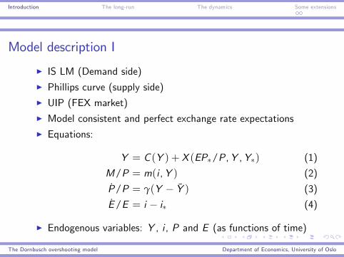
Model description I

I IS LM (Demand side)I Phillips curve (supply side)I UIP (FEX market)I Model consistent and perfect exchange rate expectationsI Equations:

Y = C (Y ) + X (EP∗/P,Y ,Y∗) (1)

M/P = m(i ,Y ) (2)

P/P = γ(Y − Y ) (3)

E/E = i − i∗ (4)

I Endogenous variables: Y , i , P and E (as functions of time)



Model description II

I Exogenous variables: Y∗, P∗, i∗, MI Initial condition: P(0) = P0

Because this is a more complex dynamic model, it is useful to lookat the long-run solution first, assuming that the long-run solutioncorresponds to a stable steady-state of the dynamic model.

I This simplifies the analysis of the long-run effects ofexogenous changes (which we are interested in).

I But the relevance of the answers hinges on the assumedstability, so have to come back to the stability issue.



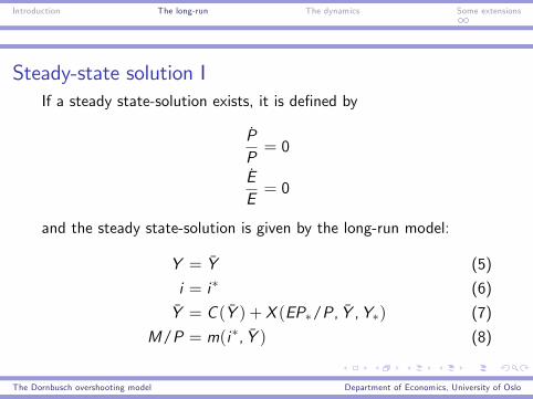
Steady-state solution IIf a steady state-solution exists, it is defined by

PP= 0

EE= 0

and the steady state-solution is given by the long-run model:

Y = Y (5)

i = i∗ (6)

Y = C (Y ) + X (EP∗/P, Y ,Y∗) (7)

M/P = m(i∗, Y ) (8)



Steady-state solution II

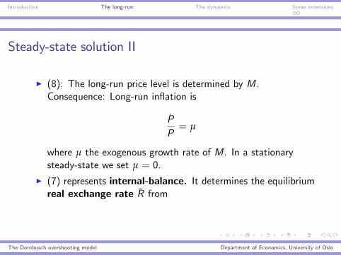
I (8): The long-run price level is determined by M.Consequence: Long-run inflation is

PP= µ

where µ the exogenous growth rate of M. In a stationarysteady-state we set µ = 0.

I (7) represents internal-balance. It determines the equilibriumreal exchange rate R from



Steady-state solution III

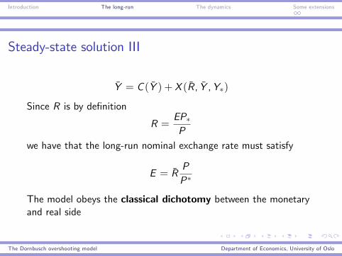
Y = C (Y ) + X (R, Y ,Y∗)

Since R is by definition

R =EP∗P

we have that the long-run nominal exchange rate must satisfy

E = RPP∗

The model obeys the classical dichotomy between the monetaryand real side



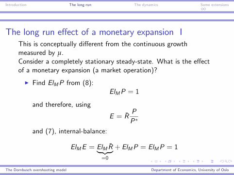
The long run effect of a monetary expansion IThis is conceptually different from the continuous growthmeasured by µ.Consider a completely stationary steady-state. What is the effectof a monetary expansion (a market operation)?

I Find ElMP from (8):ElMP = 1

and therefore, using

E = RPP∗

and (7), internal-balance:

ElME = ElM R︸︷︷︸=0

+ ElMP = ElMP = 1



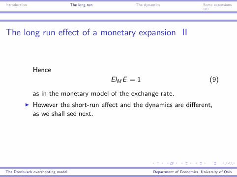
The long run effect of a monetary expansion II

HenceElME = 1 (9)

as in the monetary model of the exchange rate.

I However the short-run effect and the dynamics are different,as we shall see next.



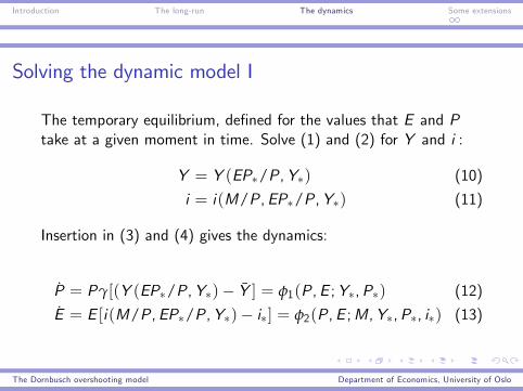
Solving the dynamic model I

The temporary equilibrium, defined for the values that E and Ptake at a given moment in time. Solve (1) and (2) for Y and i :

Y = Y (EP∗/P,Y∗) (10)

i = i(M/P,EP∗/P,Y∗) (11)

Insertion in (3) and (4) gives the dynamics:

P = Pγ[(Y (EP∗/P,Y∗)− Y ] = φ1(P,E ;Y∗,P∗) (12)

E = E [i(M/P,EP∗/P,Y∗)− i∗] = φ2(P,E ;M,Y∗,P∗, i∗) (13)



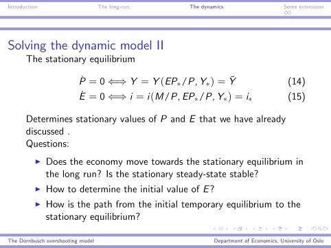
Solving the dynamic model IIThe stationary equilibrium

P = 0⇐⇒ Y = Y (EP∗/P,Y∗) = Y (14)

E = 0⇐⇒ i = i(M/P,EP∗/P,Y∗) = i∗ (15)

Determines stationary values of P and E that we have alreadydiscussed .Questions:

I Does the economy move towards the stationary equilibrium inthe long run? Is the stationary steady-state stable?

I How to determine the initial value of E?I How is the path from the initial temporary equilibrium to thestationary equilibrium?



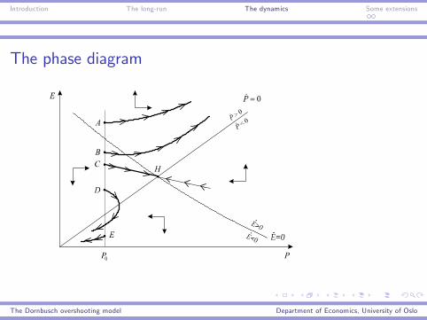
The phase diagram



Deriving the phase-diagram for P and E I

I Internal-balance: The P = 0-locus

P = 0⇐⇒ Y = Y (EP∗/P,Y∗) = Y

I Y depends on ratio P/E . To keep Y constant at Y , E mustincrease proportionally with P.

I P above P = 0 means Y low, P declining

I The E = 0-locus

E = 0⇐⇒ i(M/P,EP∗/P,Y∗) = i∗

∂E∂P |E=0

=iM/P

MP + iRRiRR

PE, iM/P < 0, iR > 0



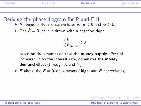
Deriving the phase-diagram for P and E III Ambiguous slope since we have iM/P < 0 and iR > 0.I The E = 0-locus is drawn with a negative slope

∂E∂P |E=0

< 0

based on the assumption that the money supply effect ofincreased P on the interest rate, dominates the moneydemand effect (through R and Y ).

I E above the E = 0-locus means i high, and E depreciating



Deriving the phase-diagram for P and E III

I In the phase-diagram, the arrows point away from E = 0 andtowards P = 0.

I H is stationary equilibrium

I Starting point anywhere on P0-line

I A, B accelerating inflation forever

I D, E accelerating deflation until i = 0

I C saddle path leading to stationary equilibrium



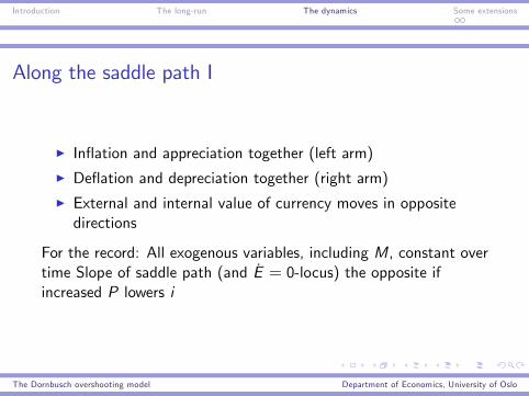
Along the saddle path I

I Inflation and appreciation together (left arm)

I Deflation and depreciation together (right arm)

I External and internal value of currency moves in oppositedirections

For the record: All exogenous variables, including M, constant overtime Slope of saddle path (and E = 0-locus) the opposite ifincreased P lowers i



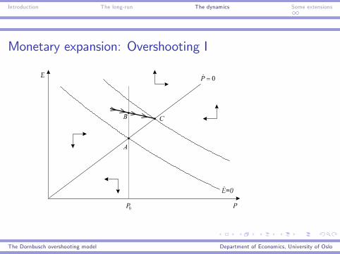
Monetary expansion: Overshooting I



I Starting from AI Locus for internal balance unaffectedI Locus for E = 0 shifts upwardsI Same price level, lower interest rate, higher E needed to keepmoney market in equilibrium

I C new stationary equilibrium

I Look for saddle path leading to CI Immediate depreciation from A to BI Gradual appreciation from B to CI Along with gradual inflation and i < i∗



The short-run effect overshooting the long-run effect I

I Occurs because P is a predetermined variable that changegradually over time (not a jump variable)

I Also happens in response to shocks to money demand orforeign interest rates

I Increases the short-run effect on output of monetarydisturbances

I May explain the high volatility of floating ratesI Empirical evidence mixedI May occur in other flexible prices too?



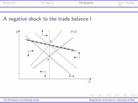
A negative shock to the trade balance I



I Real-depreciation needed to keep Y at Y constant

I P = 0-locus shifts up

I Same depreciation keeps i = i∗(by keeping money demandconstant)

I E = 0-locus shifts up equally

I Nominal exchange rate jumps from A to B

I No dynamic adjustment process in this case



Summary of results and caveat I

I A floating exchange rate insulates against demand shocksfrom abroad

I A floating exchange rate also stops domestic demand shocksfrom having output effects

Caution!

I Studied only permanent shocksI Less damping of temporary shocks (see Ch 6.4)I Less damping if money supply deflated by index containingforeign goods

I Structural change may meet real obstacles



Extending the analysis I

I Can be solved for any time paths for the exogenous variables.

I (Log)linearization necessary for closed-form solutions. (OR Ch9))

I As in monetary model, the present exchange rate depends onthe whole future of the exogenous variables.

I Phillips-curve witthout expectations is problematic in aninflationary environment.



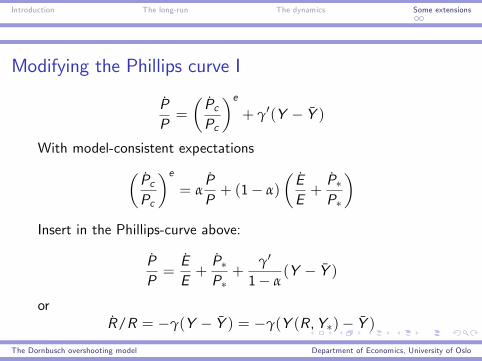
Modifying the Phillips curve I

PP=

(PcPc

)e+ γ′(Y − Y )

With model-consistent expectations(PcPc

)e= α

PP+ (1− α)

(EE+P∗P∗

)Insert in the Phillips-curve above:

PP=EE+P∗P∗+

γ′

1− α(Y − Y )

orR/R = −γ(Y − Y ) = −γ(Y (R,Y∗)− Y )



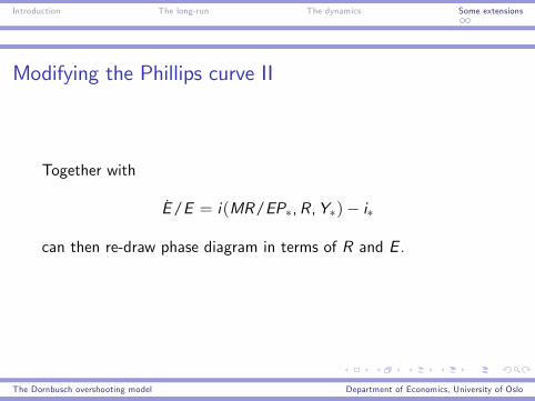
Modifying the Phillips curve II

Together with

E/E = i(MR/EP∗,R,Y∗)− i∗

can then re-draw phase diagram in terms of R and E .



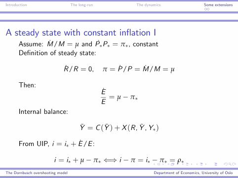
A steady state with constant inflation IAssume: M/M = µ and P∗P∗ = π∗, constantDefinition of steady state:

R/R = 0, π = P/P = M/M = µ

Then:EE= µ− π∗

Internal balance:

Y = C (Y ) + X (R, Y ,Y∗)

From UIP, i = i∗ + E/E :

i = i∗ + µ− π∗ ⇐⇒ i − π = i∗ − π∗ = ρ∗



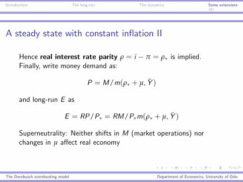
A steady state with constant inflation II

Hence real interest rate parity ρ = i − π = ρ∗ is implied.Finally, write money demand as:

P = M/m(ρ∗ + µ, Y )

and long-run E as

E = RP/P∗ = RM/P∗m(ρ∗ + µ, Y )

Superneutrality: Neither shifts in M (market operations) norchanges in µ affect real economy



Wider implications

Fixed versus floating exchange rates IAssuming (close to) perfect capital mobility in both cases

I Floating dampens the output effects of demand shocksI Floating speeds up the demand response to shocks topotential output

I Fixed rate insulates the real economy from monetary shocksI Fixed rates dampen the output response to pure cost-pushshocks

I Shocks from exchange rate expectations / risk premium -difference can go either way

I fixed - main impact through interest rateI floating - main impact through exchange rateI effects have opposite sign



Wider implications

Fixed versus floating exchange rates II

Fixed versus floating exchange rates:Does one regime lead to more noise than the other?

I Different credibility of fixed M and fixed E?

I Floating exchange rates require good forecasting abilities

Floating with inflation target is different from floating with moneysupply target.


Documents

The Dornbusch overshooting model - Universitetet i · PDF fileIntroductionThe long-runThe dynamics Some extensions The Dornbusch overshooting model 4330 Lecture 8 Ragnar Nymoen Department