Productivity Overshooting: The Dynamic Impactof Trade Opening with Heterogeneous Firms�

Thomas Chaneyy

University of Chicago and NBER

June, 2005

Abstract

In this paper, I build a dynamic model of trade with heterogeneous �rms which extendsthe work of Melitz (2003). As countries open up to trade, they will experience a productivityovershooting. Aggregate productivity increases in the long run, but it increases even more soin the short run. When trade opens up, there are too many �rms, inherited from the autarkyera. The most productive foreign �rms enter the domestic market. Competition is �erce. Theleast productive �rms that are no more pro�table are forced to stop production. Not only dothe most productive �rms increase their size because they export, but the least productive�rms stop producing altogether. Aggregate productivity soars. As time goes by, �rms start toexit because of age. Competition softens. Some less productive �rms resume production. Thispulls down aggregate productivity. The slower the exit of �rms, the larger this overshootingphenomenon. This model also predicts that the price compression that accompanies tradeopening may be dampened in the long run. It also predicts that inequalities should increaseat the time when a country opens up to trade, and then gradually recede in the long run.

�I am grateful to Marc Melitz, Xavier Gabaix and Daron Acemo�glu for their constant encouragements and theiradvice. All remaining errors are mine. First draft: June 2005.

yContact: Department of Economics, The University of Chicago, Chicago, IL 60637. Email:tchaney@uchicago.edu.

1

1 Introduction

There are strong empirical evidences that trade opening induces massive reallocations of the

factors of production, not only between sectors, but also between individual �rms within a given

sector. In a series of papers, Bernard and Jensen (1999, 2001a, 2001b, 2002) acknowledge the

importance of those reallocations between �rms, and the importance of heterogeneity between

�rms with regard to exports. Bernard, Eaton, Jensen and Kortum (2003) show that di¤erences

in productivity among �rms may explain the patterns of international trade. Exporters are

more productive, larger, and more capital intensive than non exporters. Using a panel of French

�rms, Eaton, Kortum and Kramarz (2004a, 2004b) document the large di¤erences in size and

productivity between exporters and non exporters, and between multiple countries exporters and

single country exporters. The reallocation of the factors of production from low productivity

�rms towards high productivity exporters when trade is opened up accounts for large variations

in aggregate volatility.

There is little understanding of the transitional dynamics following trade opening. Empirically,

we do observe that the short run impact of trade opening is much larger than the long run impact.

The exit of �rms in import competing sectors following a trade liberalization is typically large,

but short lived. Many adjustments that are typical of trade liberalization episodes seem to be

stronger in the short run than in the long run.

I build a dynamic model of international trade with heterogeneous �rms that helps explain the

dynamics of productivity after a country opens up to trade. As countries open up to trade, they

will experience a productivity overshooting. Aggregate productivity increases in the long run,

but it increases even more so in the short run. When trade opens up, there are too many �rms,

inherited from the autarky era. The most productive foreign �rms enter the domestic market.

Competition is �erce. The least productive �rms that are no more pro�table are forced to stop

production. Not only do the most productive �rms increase their size because they export, but

the least productive �rms stop producing altogether. Aggregate productivity soars. As time goes

by, �rms start to exit because of age. The competitive situation improves. Some less productive

�rms resume production. This pulls down aggregate productivity. The slower the exit of �rms,

and the more competitive the economy, the larger this overshooting phenomenon. This model

also predicts that the price compression that accompanies trade opening may be dampened in the

long run. It also predicts that inequalities should increase at the time when a country opens up

2

to trade, and then gradually recede in the long run.

This model extends the pioneering work on trade with heterogeneous �rms of Marc Melitz

(2003). Melitz describes the long run impact of trade opening. He only considers the steady state

properties of such a model with heterogeneous �rms. By considering the transitional dynamics,

I am able to see how di¤erences between the mass of �rms in the short run and in the long run

may lead to a non monotonic response of aggregate productivity along the transition towards

the new steady state. Hopenhaym (1992) also describes the reallocation of production between

�rms in an dynamic model, but considers only long run predictions. Eaton and Kortum (2002)

develop a model of international trade with heterogeneous �rms which extends the framework

of Dornbusch, Fischer and Samuelson (1977) to a multi country setting. They only describe the

steady state properties of this model.

The model most closely related to this is Ghironi and Melitz (2005). They analyze the tran-

sitional dynamic in a model of trade with heterogeneous �rms. They �nd that �rm heterogeneity

may explain systematic departures from purchasing power parity, and provides microfoundations

for the Harrod-Balassa-Samuelson e¤ect. In their model, they impose by assumption that no �rm

will be forced to exit their domestic market when trade is opened up. The only dynamic comes

from the entry and exit of �rms into the export market, and the exogenous natural death among

�rms. In addition, Ghironi and Melitz have to rely on numerical simulations to derive dynamics.

I adopt a di¤erent formalization that allows me to account for the large exit of �rms at times

of trade liberalizations. I am able to describe analytically the transition towards a steady state

where some �rms are allowed to resume production.

The mechanism generating productivity overshooting is intimately related to the overshooting

model of Rudiger Dornbusch (1976). Technically, it takes more time for the number of �rms to

adjust than for the relative size of �rms. This is what explains the di¤erence between short run

and long run adjustments. In the short run, the number of �rms cannot adjust discretely beyond

a certain point. It only evolves sluggishly, as �rms start dying. Therefore, in the short run, the

relative size of �rms must adjust in order to clear the labor market. The size of less productive

�rms shrinks whereas that of more productive �rms increases. This shift of mass towards the

most productive �rms explains the large increase of aggregate productivity in the short run. As

time goes by, the number of �rms gradually adjusts, and the size of less productive �rms increases

faster than that of more productive ones. Aggregate productivity falls towards its long run steady

state.

3

The remainder of the paper is organized as follows. Section 2 introduces a simple dynamic

model of trade with heterogeneous �rms. Section 3 describes the transitional dynamics when

trade is opened up. Section 4 concludes.

2 A simple model of trade with heterogeneous �rms

I build up a simple model of trade with heterogeneous �rms based on Melitz (2003). For simplicity,

I use similar notations as the ones used by Melitz, and I add new ones only when necessary.

The world is comprised of two identical countries, home and foreign. I will only consider

symmetric equilibria.1 Each country is populated with a mass L of workers. Those workers

produce goods, earn wages and dividends, and consume. For simplicity, I assume that all workers

own a single share in a mutual fund. The mutual fund owns all domestic �rms, collects all

their pro�ts, invests in new �rms when optimal, and redistributes all remaining pro�ts to the

workers. There are no international capital markets.2 Perfect competition on the labor market,

and identical ownership in the mutual fund allow me to consider that everything is as if all

decisions were undertaken by a representative consumer.

2.1 Demand

Each worker is endowed with one unit of labor that she supplies inelastically. I normalize wages

(equal across countries) to one, and express all prices in terms of wages. Workers share the same

intertemporal utility. They consume a CES aggregate of di¤erentiated goods in each period. If

they consume a quantity qt (') of variety ' in period t, and all varieties in the set �t, they derive

a utility, U0 � E0�P+1

t=0 �tCt�,with Ct =

�R'2� qt (')

��1� d'

� ���1. The elasticity of substitution

between any two varieties is constant and equal to �, � is a subjective discount factor. For

simplicity, I will consider the limiting case where � !�<1

1, so that everything is as if � = 1,

but the intertemporal utility is still well de�ned. The price Pt of one unit of the composite

good C depends on the price of each variety: Pt =�R'2�t pt (')

1�� d'� 11��, where �t is the

endogenous set of available goods. Given those isoelastic preferences, the representative consumer

will spend a fraction of its income on each di¤erentiated variety. How much of each variety she

1This assumption, as in Melitz (2003) simpli�es the analysis greatly, since it prevents relative wages fromadjusting.

2Note that the symmetry assumption makes international �nancial markets irrelevant.

4

consumes depends on the price of this variety relative to the price of others. The information

about the price of all other varieties is summed up in the price of the composite consumption

good Pt. If total expenditure on di¤erentiated goods is Rt, the representative consumer spends

rt (') = Rt (pt (') =Pt)1�� on variety '.

2.2 Production and trade

Labor is the only factor of production. Production is done under increasing returns to scale. Each

�rm must pay an overhead cost each period. This �xed per period cost is identical for all �rms.

Firms are heterogeneous in terms of productivity. The marginal cost of production is constant

for each �rm, but di¤ers across �rms. Each �rm draws a random labor productivity shock ',

meaning that the unit labor requirement is equal to 1='. For simplicity, the productivity of a

�rm is �xed upon entry, and does not evolve over the life-span of the �rm. The cost of producing

q units of goods for a �rm with productivity ' is c (') = f + q='.

When trade is allowed between the two countries, there are two types of trade barriers: a

�xed cost and a variable cost. In order to enter the foreign market, a �rm must pay a �xed cost

fx. For simplicity, I assume that this �xed cost is paid each period. Having a sunk entry cost

into the foreign market in addition to a �xed per period cost would not change the dynamics

fundamentally. It would only slow down the adjustments of trade �ows following the opening to

trade between the two countries.3 The variable trade cost is a traditional "iceberg" transportation

cost. If 1 unit of good is shipped between the two countries, only a fraction 1=� arrives. The

larger � , the more expensive transportation.

Each �rm is a monopolist for its own variety. If it does export, it is allowed to charge di¤erent

prices in each market. Given the production technology, and the technology of transportation

for international trade, and given that demand is isoelastic, �rms will charge a constant mark-up

over marginal cost. A �rm with productivity ', if it does survive, will charge a price pd (') on

the domestic market; if it does export, it will charge a price px (') on the foreign market:

pd (') =1

�'and px (') =

�

�'(1)

with 1� =

���1 > 1 the mark-up charged by each �rm.

3Outside of steady state, and unlike in Melitz (2003), it does matter whether the �xed cost of exporting is paidonce and for all or at the beginning of each period. Those two formulations won�t be equivalent anymore. I assumethe cost is paid each period, which simpli�es greatly the computation of the transitional dynamics. I believe resultswould not change qualitatively if I opted for the other formulation.

5

I de�ne the distribution of �rm productivity at time t by �t (�), with all �rms above produc-

tivity '�t selling on the domestic market, and all �rms with a productivity above '�x;t exporting.

Both the sequence of �t�s and of f'�; '�xgt�s will be determined in equilibrium. Plugging the prices

set by each individual �rm from Eq. 1 into the price index, aggregate prices at time t are de�ned

by,

(�Pt)1�� =

+1Z'�t

'��1�t (') d'+

+1Z'�x;t

�'�

���1�t (') d' (2)

I can therefore compute quantities sold by each �rm, both at home and abroad, pro�ts earned

by �rms, and from these pro�ts, I know the set of �rms that are able to survive, and the set

of �rms that are able to export.4 At time t, a �rm with productivity ', if it does produce at

all, produces for the domestic market a quantity qd;t (') = RtPt(Pt�')

�, so that its total domestic

sales are rd;t (') = Rt (Pt�')��1, and the total pro�ts it earns from selling domestically are

�d;t (') =rd;t(')� � f . If this �rm is able to export, it produces for the foreign market a quantity

qx;t (')f:o:b: =RtPt

�Pt�'�

��(or including the shipping cost, qx;t (')c:i:f: =

�RtPt

�Pt�'�

��), so that its

total foreign sales are rx;t (') = Rt

�Pt�'�

���1, and the total pro�ts it earns from exporting are

�x;t (') =rx;t(')� � fx.

Assumption 1 In any period, a �rm may decide not to produce any quantity. In such a case, it

does not have to incur the overhead cost. In other words, a �rm that wants to survive does not

have to earn negative pro�ts in order to stay in business.5

As in Melitz, I can de�ne thresholds for domestic production, and for exports. No �rm will

produce quantities if it means earning non positive pro�ts, and no �rm will export if it means

earning non positive pro�ts from exporting. I de�ne '�t as the productivity of the least productive

�rm earning non negative pro�ts from domestic sales: �d;t ('�t ) = 0. By the same token, '�x;t is the

productivity of the least productive �rm earning non negative pro�ts from exporting: �x ('�x) = 0.

I solve for the thresholds '�t and '�x;t. The conditions de�ning those threshold are the zero cuto¤

4Note that I use the productivity ' as the identity of a �rm. Literally, there is zero mass of �rms with aproductivity exactly equal to '. In this continuum setting, we can say that the number of �rms with a productivity' is equal to � (') d', the density at '. So potentially, there are "more than one" single �rm with such a productivity.Formally, each of these �rms has a di¤erent identity (each of them produces a unique di¤erentiated variety). Howeverthey all behave in exactly the same way. They are indistinguishable from their actions. Hence I can safely abuselanguage and identify a �rm by its productivity, '.

5This assumptions insures that the distribution of productivity among surviving �rms is stationary. It greatlysimpli�es the description of the dynamic adjustments after opening to trade. I discuss relaxing this assumption(and forcing �rms to pay overhead costs each period in order to stay in business) in appendix A.

6

pro�t conditions (domestic and foreign):

'���1t =�f

Rt� (�Pt)1�� (ZCPt)

'���1x;t =�fxRt

���Pt�

�1��=

����1

fxf

�� '���1t (ZCPx;t)

Any �rm with a productivity below '�t will not produce for the domestic market, and no �rm

with a productivity below the threshold '�x;t will export.6 From those productivity thresholds, I

can de�ne the probability of exporting, conditional on survival: px;t =P('>'�x;t)P ('>'�t )

.

2.3 Entry and exit of �rms

The distribution of �rms at any point in time is the result of a history of entry and exit of �rms.

Entry is done in the following way. An entrepreneur may decide to start up a �rm. In order

to do so, she must pay a sunk entry cost fe. Once this cost is paid, she receives a productivity

shock ', drawn from a random distribution with c.d.f. g (�) and p.d.f. G (�) de�ned over the

support ['min;+1).7 Any �rm that does not expect to earn positive pro�ts in the future exits.

In addition, all surviving �rms have an exogenous probability � of dying each period.

I assume free entry. If a �rm with productivity ' earns total pro�ts �t (') in period t (domestic

pro�ts, which may be equal to zero at some points in time, plus, for some �rms, export pro�ts),

then the free entry condition at date t states that if there are �rms that enter at time t, the value

of entering, ve;t, must equal the cost of entering, fe,

ve;t =

+1Z'min

+1Xs=t

(1� �)s�t �s (')!g (') d' � fe (FEt)

If fe >R +11

�P+1s=t (� (1� �))

s�t �s (')��t (') d', no �rm enters. Free entry prevents the

other strict inequality from ever happening. Condition FEt holds with equality as long as a

strictly positive number of �rms do enter. Note that it will be crucial to de�ne the pro�t function

�t (�). This function is potentially complex along the transition following opening to trade. Firms6 I assume that fx

f���1 > 1. Trade barriers are always su¢ ciently high so that only a subset of �rms export:

'�t < '�x;t. If this condition were violated, then '�t = '�x;t. All active �rms would export, and all results would

carry through.7The only condition on the distribution of productivity shocks is that the (� � 1)th moment of G is de�ned, or

that the integralR +1'min

'��1g (') d' converges. This property ensures that the total size of the economy is �nite.The choice of 'min is purely arbitrary. The assumption that the support for this distribution is unbounded fromabove simpli�es notations greatly, but it is only a notational assumption. It is perfectly admissible within thismodel that there is zero mass above a certain threshold 'max (g (') = 0; 8' > 'max).

7

may not earn any pro�t over some period of time, and then start earning positive pro�ts. After

some point in time, they may even start earning some extra pro�ts from exporting.

The free entry condition and the general equilibrium will determine how many �rms enter

each period. Call Me;t the number of new entrants at time t. I must now impose that the labor

market clears. Labor is used for investment (to cover the sunk entry cost of new entrants), and

for production. The labor allocated to production is used both to pay for the �xed costs (�xed

overhead cost for domestic production plus �xed trade barrier if the �rm exports), and to cover

the variable cost of production. The total labor used for investment8 is fe�Me;t. If the there is a

total massMt of �rms operating at time t, and a fraction px;t of those �rms are exporters, the total

workforce used to cover overhead costs is (f + px:tfx) �Mt. Since each �rm charges a constant

mark-up over marginal cost, it can easily be proven that if total expenditures on di¤erentiated

goods is Rt, the total workforce used for producing di¤erentiated goods (variable cost only) is

�Rt. The labor market clearing condition at each point in time during the transition requires,

L = fe �Me;t + (f + px:tfx)�Mt + �Rt (LMCt)

I will see in the next two sections how the free entry condition characterizes the autarky and

trade steady states. I will then see how entry of new �rms take place along the transition from

the autarky steady state to a new trade steady state.

2.4 Autarky steady state

In this section and the next, I recall Melitz (2003) computation of the steady state of this economy,

both under autarky, and under trade. I will denote the autarky steady state by the time subscript

t = �1, and the trade steady state by the time subscript t = +1.

In a steady state, there is as much entry as exit. All �rm with a productivity below '��1

exit immediately upon receiving their productivity draw. Labor market clearing insures that

total expenditure on di¤erentiated goods is exactly equal to L. All pro�ts are used to invest into

starting up new �rms, so that the mutual fund�s �nances are balanced. So in the autarky steady

state, (LMC�1), R�1 = L.

Following Melitz (2003), I can de�ne a special average productivity among active �rms:

~' ('�) � R +1

'� '��1g (') d'R +1'� g (') d'

! 1��1

8 It is possible that at some point in time, there is no entry, so that Me;t = 0.

8

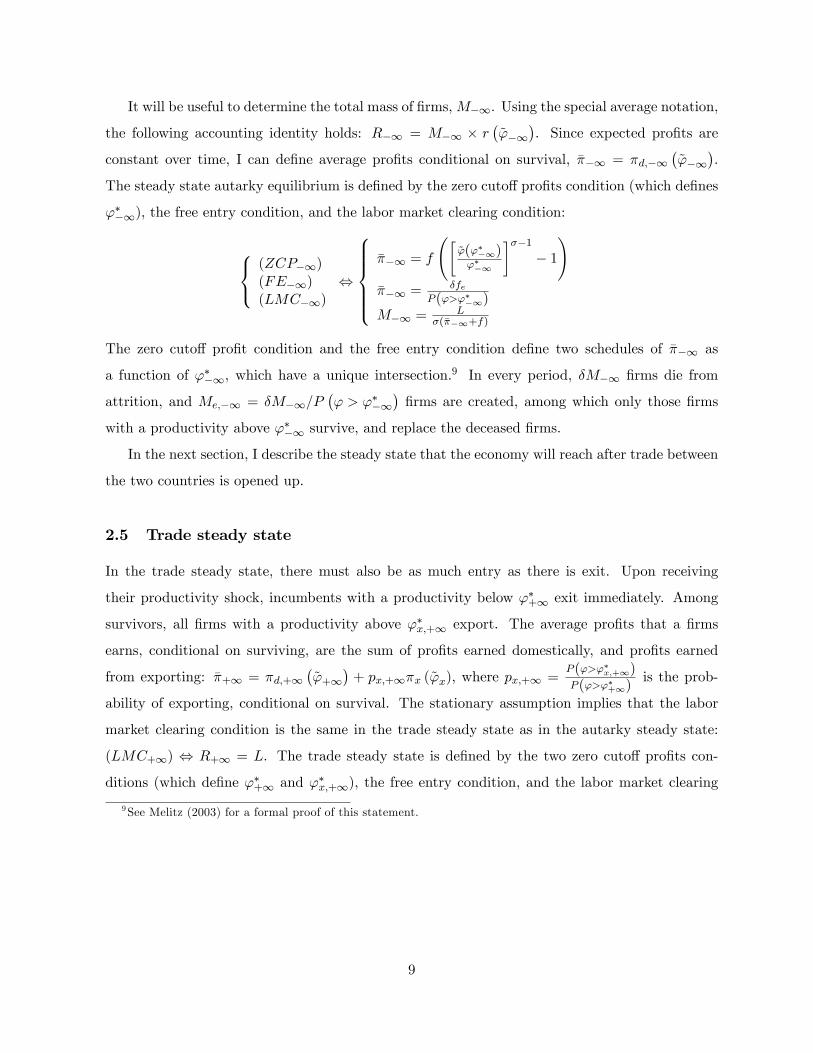
It will be useful to determine the total mass of �rms,M�1. Using the special average notation,

the following accounting identity holds: R�1 = M�1 � r�~'�1

�. Since expected pro�ts are

constant over time, I can de�ne average pro�ts conditional on survival, ���1 = �d;�1�~'�1

�.

The steady state autarky equilibrium is de�ned by the zero cuto¤ pro�ts condition (which de�nes

'��1), the free entry condition, and the labor market clearing condition:

8<:(ZCP�1)(FE�1)(LMC�1)

,

8>>>><>>>>:���1 = f

�~'('��1)'��1

���1� 1!

���1 = �feP('>'��1)

M�1 = L�(���1+f)

The zero cuto¤ pro�t condition and the free entry condition de�ne two schedules of ���1 as

a function of '��1, which have a unique intersection.9 In every period, �M�1 �rms die from

attrition, and Me;�1 = �M�1=P�' > '��1

��rms are created, among which only those �rms

with a productivity above '��1 survive, and replace the deceased �rms.

In the next section, I describe the steady state that the economy will reach after trade between

the two countries is opened up.

2.5 Trade steady state

In the trade steady state, there must also be as much entry as there is exit. Upon receiving

their productivity shock, incumbents with a productivity below '�+1 exit immediately. Among

survivors, all �rms with a productivity above '�x;+1 export. The average pro�ts that a �rms

earns, conditional on surviving, are the sum of pro�ts earned domestically, and pro�ts earned

from exporting: ��+1 = �d;+1�~'+1

�+ px;+1�x (~'x), where px;+1 =

P('>'�x;+1)P('>'�+1)

is the prob-

ability of exporting, conditional on survival. The stationary assumption implies that the labor

market clearing condition is the same in the trade steady state as in the autarky steady state:

(LMC+1) , R+1 = L. The trade steady state is de�ned by the two zero cuto¤ pro�ts con-

ditions (which de�ne '�+1 and '�x;+1), the free entry condition, and the labor market clearing

9See Melitz (2003) for a formal proof of this statement.

9

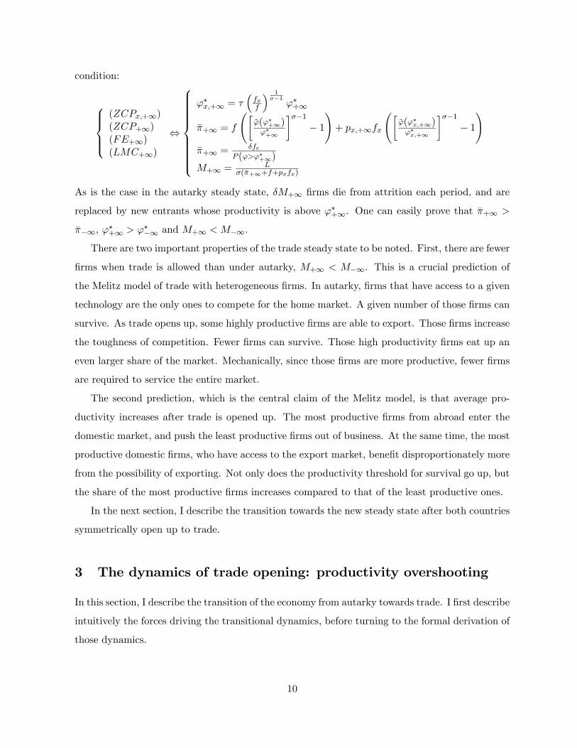
condition:

8>><>>:(ZCPx;+1)(ZCP+1)(FE+1)(LMC+1)

,

8>>>>>>>><>>>>>>>>:

'�x;+1 = ��fxf

� 1��1

'�+1

��+1 = f

�~'('�+1)'�+1

���1� 1!+ px;+1fx

�~'('�x;+1)'�x;+1

���1� 1!

��+1 = �feP('>'�+1)

M+1 = L�(��+1+f+pxfx)

As is the case in the autarky steady state, �M+1 �rms die from attrition each period, and are

replaced by new entrants whose productivity is above '�+1. One can easily prove that ��+1 >

���1, '�+1 > '��1 and M+1 < M�1.

There are two important properties of the trade steady state to be noted. First, there are fewer

�rms when trade is allowed than under autarky, M+1 < M�1. This is a crucial prediction of

the Melitz model of trade with heterogeneous �rms. In autarky, �rms that have access to a given

technology are the only ones to compete for the home market. A given number of those �rms can

survive. As trade opens up, some highly productive �rms are able to export. Those �rms increase

the toughness of competition. Fewer �rms can survive. Those high productivity �rms eat up an

even larger share of the market. Mechanically, since those �rms are more productive, fewer �rms

are required to service the entire market.

The second prediction, which is the central claim of the Melitz model, is that average pro-

ductivity increases after trade is opened up. The most productive �rms from abroad enter the

domestic market, and push the least productive �rms out of business. At the same time, the most

productive domestic �rms, who have access to the export market, bene�t disproportionately more

from the possibility of exporting. Not only does the productivity threshold for survival go up, but

the share of the most productive �rms increases compared to that of the least productive ones.

In the next section, I describe the transition towards the new steady state after both countries

symmetrically open up to trade.

3 The dynamics of trade opening: productivity overshooting

In this section, I describe the transition of the economy from autarky towards trade. I �rst describe

intuitively the forces driving the transitional dynamics, before turning to the formal derivation of

those dynamics.

10

If �rms are heterogeneous in terms of productivity, only a subset of �rms, the most productive,

are able to overcome trade barriers. The presence of these high productivity exporters, along with

the upward shift in average productivity, implies that fewer �rms can survive under trade than

under autarky. In a sense, in the autarky steady state, domestic �rms are alone to satisfy the

entire domestic demand, and many �rms must operate. When trade is opened up, there are "too

many" �rms. So during the transition, the mass of �rms must shrink.

There is a fundamental asymmetry between the creation and destruction of �rms, due to the

presence of sunk entry costs. Because I have assumed free entry, as soon as there is some potential

for pro�ts, there will always be some �rms entering. Exit on the other hand may take time. If the

mass of �rms at every level of productivity must shrink in order to reach the new steady state,

because high productivity �rms only die at a slow pace, the transition will be slow. Because

existing �rms have already paid the sunk entry cost, they are far less vulnerable than potential

entrants. They will exit if and only if they do not expect to earn any positive pro�ts at any point

in the future.

At the moment when trade is opened up, the most productive foreign �rms start exporting.

They eat up part of the domestic demand, and push many low productivity �rms out of business.

The least productive among those �rms will never be able to generate positive pro�ts ever again

in this globalized world, and exit immediately. Competition is at its �ercest right at the time

when trade is opened up. So upon opening to trade, there is a spike of destruction of �rms. This

implies a large increase in average productivity: only the most productive �rms can survive in

this new environment.

Because the world has inherited an "overcrowded" economy, there won�t be any entry of �rms

for some period of time. During this transitional period, the natural death eats up the total mass

of �rms. Competition gradually softens. Firms with a low productivity that had been on hold

until then can start producing again. Exporting becomes easier as the mass of �rms shrinks. The

mass of �rms gradually shifts towards less productive �rms that can more easily survive now.

Eventually, when the mass of �rms has shrunk su¢ ciently, the new trade steady state is

reached, with a lower average productivity than at the time of trade opening. Once this state is

reached, entry starts again. One important property of this model is that the dynamics towards

the trade steady state only take a �nite amount of time. This crucially depends on assumption

1, which guaranties a stationary distribution of �rm productivity.

In the next three sections, I derive formally the transitional dynamics, and their properties.

11

3.1 Transitional dynamics

Before opening to trade, the economy was in an autarky steady state, de�ned in section 2.4. Trade

opens up at time t = 0. The opening is unexpected. Because of the dynamic nature of the model,

there may be multiple rational expectations equilibria. I will only consider a class of dynamic

equilibria, those that converge towards a steady state.

It will be useful to de�ne the following alternative measure of the mass of �rms: ~Mt =

Mt=P (' > '�t ). This measure corresponds to the mass of �rms per unit of density at each level of

productivity. It also corresponds to an ideal notion of the total number of �rms, which includes

those �rms that cannot survive (with a productivity below '�t ). Depending on the value of this

alternative measure of mass in the trade steady state, there are two possible scenarii for the

transition path. If ~M+1 � ~M�1, the transition will be immediate. The economy jumps to the

new trade steady state within one period. If ~M+1 < ~M�1 on the other hand, the transition

towards the new steady state takes a �nite time.

The reason for this is simple. If there are more �rms per level of productivity in the trade

steady state than in the autarky steady state ( ~M+1 � ~M�1), competition is softer after trade is

opened than it will be in the steady state, average pro�ts are higher than in the steady state. I

know that in the trade steady state, the discounted stream of pro�ts is exactly equal to the sunk

entry cost. Hence the appeal of extra pro�ts will attract an in�ux of new �rms, in order to restore

the free entry condition (FEt) with equality. Those �rms are spread all over the distribution

of productivity, so that the mass of �rms at each level of productivity jumps immediately to its

steady state level.

If on the other hand, there are fewer �rms per level of productivity in the trade steady state

than in the autarky steady state ( ~M+1 < ~M�1), competition is tougher after trade openes than

it will be in the new steady state, average pro�ts are lower. Since in the steady state, pro�ts are

just enough to cover the sunk entry cost, lower average pro�ts implies that no �rm will enter as

long as ~Mt � ~M+1. The natural death process gradually erodes the mass of �rms, until the mass

per level of productivity reaches its steady state level. From that point onward, the economy is

in the trade steady state, and entry resumes in order to o¤set death from attrition.

I now turn to the formal proof of these statements.First, I de�ne the criterion for fast or

slow convergence towards the steady state. This criterion depends on whether the economy is

overcrowded after trade is opened up or not.

12

Criterion 2 (Overcrowding)

~M+1 < ~M�1

Remarks: If criterion 2 is met, there are more �rms at every level of productivity in the autarky

steady state than in the trade steady state (the economy is "overcrowded"), then the convergence

towards the new steady state will take some �nite amount of time, and there is overshooting in

productivity. If criterion 2 is not met, then the economy immediately adjusts to its new trade

steady state. See appendix B for the full functional form of this criterion.

Proposition 3 If criterion 2 is not satis�ed, that is if ~M+1 � ~M�1, there is an in�ux of �rms

upon trade opening: Me;0 =�~M+1 � ~M�1

�+ � ~M�1. From period t = 1 onward, the economy

is in the trade steady state de�ned in section 2.5. The productivity thresholds immediately jump

to their steady state values, '�0 = '�+1, and '

�x;0 = '

�x;+1.

Proof. It is su¢ cient to prove that when trade is allowed and Me;t = 0, ~Mt < ~M+1 )

P (' > '�t ) ��t > P�' > '�+1

���+1.

Assume, as proven in appendix B, that this property holds.

If ~M0 = ~M+1, the economy has already reached its new steady state, and no further adjust-

ment occurs.10

If the mass of �rms per level of productivity were strictly lower than its trade steady state

value, ~M0 < ~M+1, total expected pro�ts would be larger than the sunk entry cost:

ve;0 =Xt�0

(1� �)t � P (' > '�0) ��t

> ve;+1 =Xt�0

(1� �)t � P�' > '�+1

���+1 = fe

Free entry prevents the occurence of such an imbalance. So there will be a net entry of new

�rms that increases the mass of �rms to its steady state level. In order to reach the trade steady

state mass of �rms, those �rms destroyed by attrition must be replaced by new entrants: � ~M�1

must enter. In addition, the ideal mass of �rms�~M�must be increased to ~M+1, from ~M�1. So

the total number of entrants isMe;0 =�~M+1 � ~M�1

�+� ~M�1. From t = 1 onward, we are in the

trade steady state, and new �rms enter only to replace attrition deaths: Me;t =Me;+1 = � ~M+1.

Along this path, expected pro�ts and survival thresholds are constant, P (' > '�0) ��0 = ::: =

P�' > '�+1

���+1, so that the free entry condition (FEt) is satis�ed with equality for all t � 0.

10This will be the case with Pareto distributed productivity shocks.

13

Proposition 4 If criterion 2 is satis�ed, that is if ~M+1 < ~M�1, there a �nite length of time

T � 0 during which no �rm enters. At time t = T , the trade steady state de�ned in section 2.5 is

reached. T is uniquely de�ned as the minimum integer such that ~MT � ~M+1.

Proof. Assume, as proven in appendix B, that whenMe;t = 0, ~Mt > ~M+1 ) P (' > '�t ) ��t <

P�' > '�+1

���+1.

I need to prove that 8><>:Me;0 =Me;1 = ::: =Me;T�1 = 0

Me;T =�~M+1 � ~MT�1

�+ � ~MT�1

Me;T+1 = ::: =Me;+1 = � ~M+1

9>=>;is a rational expectations equilibrium. To do so, I prove that if �rms expect that the economy

will follow this path, indeed their entry decisions will follow these patterns.

As long as no entry takes place, the mass of �rms evolves according to the following law of

motion,

~Mt = (1� �) ~Mt�1 (Mt)

or ~Mt = (1� �)t ~M�1. The mass of �rms steadily declines. De�ne T as the minimum integer

such that ~MT � ~M+1. Since ~M�1 > ~M+1 > 0, since ~Mt is strictly decreasing in t and converges

towards zero, T is uniquely de�ned.11 By de�nition of T , I know that ~M0 > ::: > ~MT�1 > ~M+1 �~MT :

I now prove recursively that:

"at t = T�1, no �rm enters if agents expect the equilibrium path to be followed after t = T�1"

"at t = T�2, no �rm enters if agents expect the equilibrium path to be followed after t = T�2"

"..."

"at t = 0, no �rm enters if agents expect the equilibrium path to be followed after t = 0"

From ~MT�1 > ~M+1 ) P (' > '�t ) ��t < P�' > '�+1

���+1, I know that P

�' > '�T�1

���T�1 <

P�' > '�+1

���+1. If agents expect the equilibrium path to be followed after t = T � 1, from the

free entry condition in the trade steady state (ve;+1 = fe), I know that,

ve;T�1 =Xt�T�1

(1� �)t P (' > '�t ) ��t

= P�' > '�T�1

���T�1 + (1� �) ve;+1 < fe

11 I consider the interesting case where T > 0. If T = 0, the adjustment to the new steady state is immediate. Itis always possible to change the unit of observation for time, and hence to reduce � su¢ ciently so that T > 0:

14

So if agents expect the equilibrium path to be followed after t = T �1, no �rm enters at t = T �1:

By the same reasoning, if agents expect the equilibrium path to be followed after t = T � 2,

P�' > '�T�2

���T�2 < P

�' > '�+1

���+1, and no �rm enters at t = T � 2.

No �rm enters until t = T , and from that point onward, the economy is in steady state.

Along the transition, the equilibrium will be determined by the zero cuto¤ pro�t conditions,

the labor market clearing condition, and the law of motion for the mass of �rms. Once the steady

state is reached, the law of motion of the mass of �rms is replaced by the free entry condition:

0 � t < T

8>><>>:(ZCPt)(ZCPx;t)(Mt)

(LMCt)

t � T

8>><>>:(ZCPx;+1)(ZCP+1)(FE+1)(LMC+1)

As can be guessed from the description of the dynamic evolution of average pro�ts and the

mass of �rms, the productivity threshold jumps upon opening to trade, and then gradually falls

towards its steady state level. I describe this phenomenon of productivity overshooting in the

next section.

3.2 Productivity overshooting

In this section, I will only consider the interesting case where transitional dynamics are not

collapsed into one single period.

As trade opens up, there are too many �rms. Competition is �erce, pro�ts are low. Many

�rms are forced to stop producing, since they could not even cover their overhead costs. Only the

most productive �rms are still active, and the most productive among them are exporters. As

time goes by, since no �rm enters during the transition, �rms at every level of productivity start

dying. For the survivors, the situation gradually improves. This means that some �rms can start

exporting. Those new exporters experience a discrete increase in the volume of their sales, and

their employment. As the productivity threshold for exports falls, mass is shifted towards those

less productive exporters. At the same time, some �rms that had stopped producing altogether

15

resume their production. Some of the varieties that had disappeared when the most productive

foreign exporters had entered start being produced again. The threshold for domestic sales falls.

Aggregate productivity, measured as a size-weighted average of productivities across �rms,

falls down for two reasons. First, those �rms that resume production have a low productivity,

and they pull down average productivity. At the same time, the mass of sales is shifted gradually

away from the high productivity exporters towards the new lower productivity exporters. So as

more and more �rms die, aggregate productivity falls as well. Eventually, the economy reaches

its steady state when productivity stays constant.

Following trade opening, aggregate productivity increases in the long run. This is the main

prediction of the Melitz model. I predict that in the short run, productivity will increase more

than in the long run. This rapid increase in productivity followed by a gradual deterioration

of productivity is what I call productivity overshooting. The forces driving this overshooting

in productivity are very similar in spirit to the forces driving exchange rate overshooting in

Dornbusch (1976). In that model, the reason why exchange rate overshoots is because exchange

rates can adjust much faster than domestic prices. In this model, productivity overshoots because

it takes time for �rms that are already here to die. Because those existing �rms will not die

right away, something else must adjust in the meantime to o¤set the imbalances created by the

sudden entry of foreign exporters. This is done through a temporary reduction in the share of

low productivity �rms. Some of these less productive �rms stop producing altogether for some

time (until su¢ ciently many high productivity �rms have died, and the situation has su¢ ciently

improved). Some other �rms do not stop producing, but they reduce their production relative to

higher productivity �rms (which start exporting). This adjustment, the reduction in the share

of less productive �rms, can happen much faster than forcing existing �rms out. So in the short

run, this will be the only variable of adjustment. In a sense, one could say that the extensive

margin of productivity (how many levels of productivity can be active) can adjust much faster

than the intensive margin of productivity (how many �rms there are at each level of productivity).

This reduction in the share of less productive �rms in the short run will cause productivity to

increase substantially. In the longer run, as �rms die and the mass of �rms shrinks, this increase

in aggregate productivity is dampened. The death of �rms allows for the share of less productive

�rms to increase again, partially o¤setting the short run productivity gains.

Note that some �rms will exit de�nitively at the time when trade is opened up. Those are the

�rms that will not survive, even once the new steady state is reached. If criterion 2 does not hold,

16

there will actually be no overshooting, and productivity directly jumps to its steady state level.

This is because I do allow for immediate exit of �rms when trade is opened up. Firms have to pay

a �xed overhead production cost each period, and therefore some �rms, after trade is opened up,

know that they will never be pro�table again, and exit immediately. If I remove the assumption

of a �xed overhead cost, as is done in a similar setting by Ghironi and Melitz (2005), adjustments

will be even more sluggish, and productivity overshooting will be larger. In such a setting, the

prediction that the total mass of �rms must be reduced still holds. There is no possibility of

discretely adjusting this mass, so the adjustment will take much more time than in the current

model. I believe however that the prediction that opening up to trade will have a sudden negative

impact on the least productive domestic �rms is a plausible feature. It is interesting to see that

even when some �rms exit, transition towards the new steady state may still take some time, and

we may observe a phenomenon of productivity overshooting.

I will not go into the details of computing the average productivity of �rms (weighted by

the size of sales, or by employment) in the economy along the transition. I will only prove that

along the transition, as the mass of �rms shrinks, the productivity threshold for survival falls. It is

intuitive to see that as the productivity threshold falls towards its new steady state level, aggregate

productivity also falls. The following proposition proves formally the productivity overshooting

triggered by trade opening.

Proposition 5 (Overshooting) When the transition is not instantanuous, there is overshooting

in productivity,

'�0 > '�1 > ::: > '

�T = ::: = '

�+1 > '��1

Proof. We already know from Melitz (2003) that productivity is higher in the trade steady

state than in the autarky steady state: '�+1 > '��1

If criterion 2 is met, I know that the mass of �rms per level of productivity, ~Mt, will gradually

fall from its autarky level, towards its trade steady state level (at a constant rate (1� �)):

~M�1 > ~M0 > ~M1 > ::: > ~MT = ::: = ~M+1

See appendix B for a proof that ~Mt > ~Ms ) '�t > '�s:

It is important for this overshooting phenomenon to happen that the opening to trade is

unexpected. Looking at the transitional dynamics from an ex ante point of view, we can see

17

further justi�cations for this overshooting in productivity. There are too many �rms at the time

when trade is opened up. The pro�tability conditions worsen in such a way that no �rm has

any incentive to enter during the transition towards the new steady state. This implies that

entrepreneurs who started up their company before the opening to trade had formed the wrong

expectations regarding their future expected stream of pro�ts. Average realized pro�ts will fall

below their expected level for some time. Had those entrepreneurs known in advance about this

opening to trade, they would not have started up their company.12 This means that there was

overinvestment in autarky.

In other words, the "technology" of production has improved, in an ex ante expectation sense,

because there has been overinvestment in improving the available technology (creation of too many

�rms). This is why less investment (payments to start up new �rms) is required each period in the

trade steady state than in the autarky steady state. Since the economy had overinvested while in

autarky, it is natural that the opening to trade creates a temporary spike in productivity. This is

only temporary. As the economy converges towards its new steady state, there is disinvestment

(no creation of new �rms while old ones die). Thanks to the available "better technology" o¤ered

by trade, the aggregate productivity in the new steady state is higher than in autarky. But it is

lower than during the transitional period, which was a time of abundance of "capital".

3.3 Price compression and inequality

As trade opens up, the dynamics of productivity are parallel to movements in prices and in-

equalities. Such a model with heterogeneous �rms is perfectly �t for describing the impact of

trade opening on aggregate prices as well as inequalities (between �rms, in the absence of any

formalization of wage bargaining).

As trade opens up, prices are driven down by the entry of high productivity foreign exporters.

Literally speaking, since the model imposes that mark-ups are constant, no single �rm changes

the price it sets. However, low productivity/ high price �rms exit, and since the share of high

productivity/ low price �rms increases, aggregate prices fall when trade is opened up. This

fall in aggregate prices is exactly symmetrical to average productivity increases. In this model,

productivity is directly a mirror image of prices. This fall in aggregate prices happens in the long

run.12 I describe qualitatively what happens when the opening to trade is announced in advance in appendix C.

18

But exactly in the same way as there is overshooting in productivity, there will be "overcom-

pression" of prices in the short run. In the short run, only the most productive �rms are active.

So prices are pushed down substantially. As �rms exit, and as competition softens along the

transition path towards the new steady state, less productive �rms resume production. Those

�rms charge a higher price than their competitors. So average prices will "undershoot", in the

sense that there is a sudden drop of prices in the short run, and a gradual price increase in the

medium run.

Melitz (2003) points out that in the presence of �rm heterogeneity, inequalities between �rms

increase. This is due to the fact that more productive �rms bene�t from trade, whereas the

situation of less productive �rms worsens. So inequalities increase in the long run. But once

again, inequalities increase more in the short run than in the long run. There is overshooting in

inequalities. In the short run, only the very best �rms bene�t from the access to foreign markets,

whereas many less productive �rms have to incur a temporary loss in pro�ts (which goes all the

way to zero pro�ts for some time for �rms with a productivity '�+1 < ' < '�0). In the short run,

inequalities soar. In the medium run, as some �rms exit, inequalities among survivors recede,

until the new steady state is reached. Inequalities will always be higher in a trade regime than in

autarky, but less so in the long run than in the short run. It takes some time for the economy to

adapt to the new regime.

4 Conclusion

In this paper, I have shown that when a country opens up to trade, it will experience an sudden

increase in productivity, followed by a gradual reduction towards a steady state. Opening up to

trade does lead to a permanent increase of productivity, but there is an even larger increase in

the short run. I call this phenomenon productivity overshooting. The reason for this productivity

overshooting is simple. Because trade allows are more e¢ cient allocation of factors of produc-

tion, there will be fewer �rms in a globalized world than in a world composed of countries in

autarky. After countries open up to trade, the number of �rms will have to fall. However, in the

presence of sunk entry costs, such a reduction in the number of �rms takes time. In the short

run, competition is �erce, and many �rms cannot pro�tably produce. Only the most productive

�rms are active. Aggregate productivity soars. As the number of �rms gradually falls (as existing

�rms age), competition softens, and low productivity �rms are able to resume production. Ag-

19

gregate productivity gradually falls as the world economy converges towards its new steady state.

Along with this productivity overshooting, I expect to observe price compression in the short run,

followed by a gradual increase in aggregate prices, as well as an overshooting in inequalities.

References

[1] Bernard, Andrew B.; Jonathan Eaton; J. Bradford Jensen and Sam Kortum, 2003, "Plants

and Productivity in International Trade," American Economic Review, v. 93, pp. 1268-1290.

[2] Bernard, Andrew B. and J. Bradford Jensen, 1999, "Exceptional exporter performance:

cause, e¤ect, or both?", Journal of International Economics, v. 47, pp. 1�25.

[3] Bernard, Andrew B. and J. Bradford Jensen, 2001a, "Why Some Firms Export," The Review

of Economics and Statistics, v. 86 no. 2.

[4] Bernard, Andrew B. and J. Bradford Jensen, 2001b, "Who Dies? International Trade, Market

Structure, and Industrial Restructuring," NBER Working Paper # 8327 .

[5] Bernard, Andrew B. and J. Bradford Jensen, 2002, "Entry, Expansion, and Intensity in the

US Export Boom, 1987-1992," Review of International Economics, forthcoming.

[6] Dornbusch, Rudiger, 1976, "Expectations and Exchange Rate Dynamics," Journal of Political

Economy, v. 84, pp. 1161-76.

[7] Dornbusch, Rudiger; S. Fischer, and Paul A. Samuelson, "Comparative Advantage, Trade,

and Payments in a Ricardian Model with a continuum of Goods," American Economic Re-

view, vol. 67, pp. 823-839.

[8] Eaton, Jonathan; Sam Kortum, 2002, "Technology, Geography, and Trade," Econometrica,

vol. 70 no. 5 (September 2002), pp. 1741-1779.

[9] Eaton, Jonathan; Sam Kortum, and Francis Kramarz, 2004, "An Anatomy of International

Trade: Evidence from French Firms," American Economics Review, Papers and Proceedings,

forthcoming.

[10] Eaton, Jonathan; Sam Kortum, and Francis Kramarz, 2004, "Dissecting Trade: Firms, In-

dustries, and Export Destinations," NBER Working Paper 10344.

20

[11] Ghironi, Fabio, and Marc J. Melitz, 2005, "International Trade and Macroeconomic Dynamics

with Heterogeneous Firms." Working Paper.

[12] Helpman, Elhanan; Marc Melitz and Yona Rubinstein, 2004, "Trading Partners and Trading

Volumes," Working Paper.

[13] Hopenhaym, Hugo, 1992, "Entry, Exit, and Firm Dynamics in Long Run Equilibrium,"

Econometrica, v.60, pp. 621-653.

[14] Krugman, Paul. 1980. �Scale Economies, Product Di¤erentiation, and the Pattern of Trade.�

American Economic Review, vol. 70, pp. 950� 959.

[15] Melitz, Marc, 2003, "The Impact of Trade on Aggregate Industry Productivity and Intra-

Industry Reallocations," Econometrica, v. 71 no. 6 (November 2003), pp. 1695-1725.

21

Appendix

A Non stationary productivity distribution and dynamic adjust-ments

Absent assumption 1, the distribution of productivity among �rms during the transition may be

non stationary.

The reason is the following. When trade opens up, the productivity threshold for domestic

sales soars. In this paper, I have described what happens when existing �rms have the option of

not producing at all during some period, without going out of business (that is without having

to pay the sunk entry cost, get a productivity draw from a lottery, all over again). Therefore,

the exit decision was simple. All �rms with a productivity above '�+1 stay in business. because

they know that in the long run (once the trade steady state is reached), they will be able to

generate some strictly positive pro�ts. However, some of these �rms have to stay idle for some

time. If those �rms had to pay a �xed cost each period in order to stay in business, they would

have to gauge the cost of staying in business (a given number of periods with negative pro�ts),

against the expected bene�ts from staying in business (expected positive pro�ts starting up in

the future). The least productive among those �rms will exit. It is easy to prove that there is a

range of productivity�'�+1; �'0

�over which �rms exit immediately.

Let us now move along the transition. Firms die (there were too many �rms to start with),

the productivity threshold for domestic sales goes down. Eventually, this threshold goes down

below �'0. Then, with each new cohort of entrants, some �rms with a productivity below �'0 will

survive. But until that point, there were no �rms with such a low productivity, whereas there is

a strictly positive number of �rms with a productivity above �'0 that have survived. Because of

the nature of the technology, there will be as many new �rms with ' > �'0 as �rms with ' < �'0

created (up to some relative probability). But since to start with, the stock of �rms with ' > �'0

is strictly positive, and there are no �rms with ' < �'0 , there is an imbalance. The distribution

of productivity among existing �rms is no longer given by g (�) � (Constant). The distribution

is tilted towards high productivity �rms. There are disproportionately many �rms with a high

productivity. Those are the �rms that survived the opening to trade.

In such a con�guration, the steady state cannot be reached in a �nite number of periods. The

disequilibrium of the distribution towards high productivity �rms gradually fades away, as those

old �rms who survived since the time when trade was opened for the �rst time die, and are replace

22

with new cohorts.

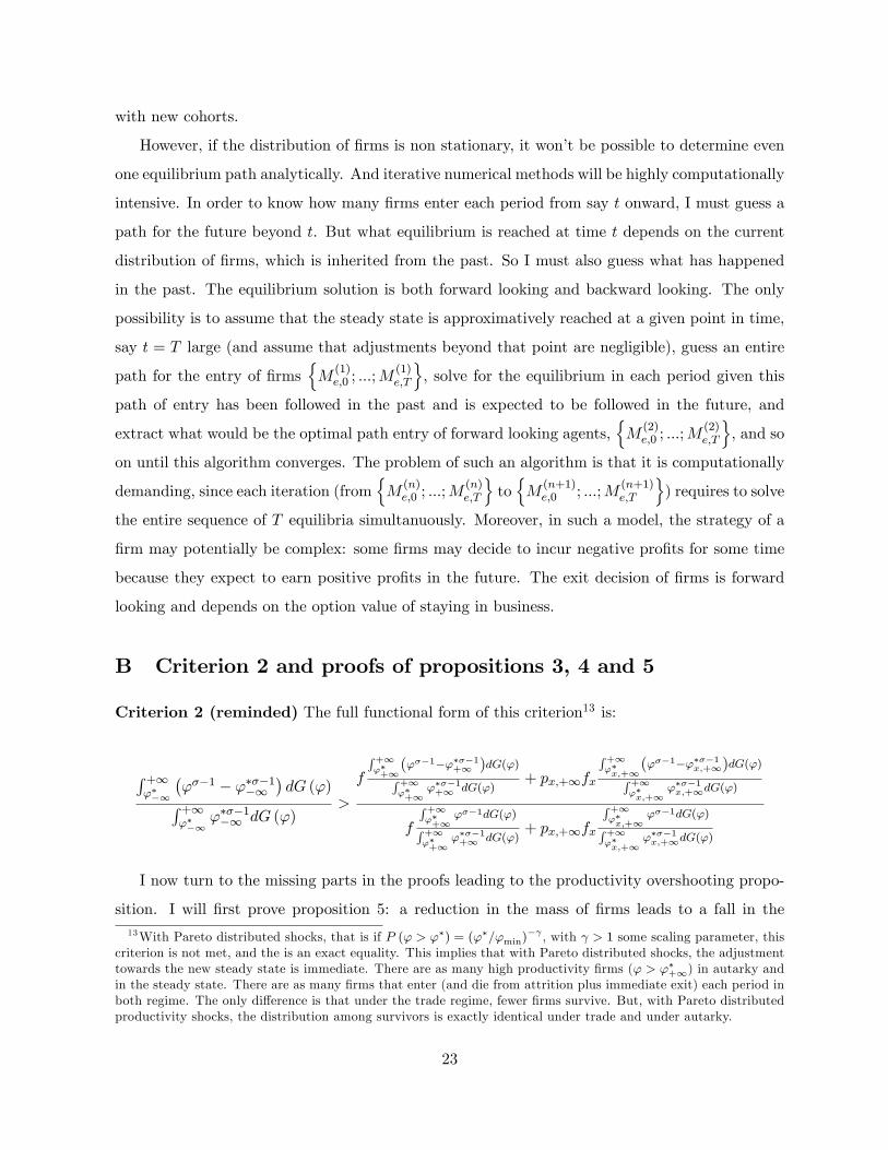
However, if the distribution of �rms is non stationary, it won�t be possible to determine even

one equilibrium path analytically. And iterative numerical methods will be highly computationally

intensive. In order to know how many �rms enter each period from say t onward, I must guess a

path for the future beyond t. But what equilibrium is reached at time t depends on the current

distribution of �rms, which is inherited from the past. So I must also guess what has happened

in the past. The equilibrium solution is both forward looking and backward looking. The only

possibility is to assume that the steady state is approximatively reached at a given point in time,

say t = T large (and assume that adjustments beyond that point are negligible), guess an entire

path for the entry of �rmsnM(1)e;0 ; :::;M

(1)e;T

o, solve for the equilibrium in each period given this

path of entry has been followed in the past and is expected to be followed in the future, and

extract what would be the optimal path entry of forward looking agents,nM(2)e;0 ; :::;M

(2)e;T

o, and so

on until this algorithm converges. The problem of such an algorithm is that it is computationally

demanding, since each iteration (fromnM(n)e;0 ; :::;M

(n)e;T

otonM(n+1)e;0 ; :::;M

(n+1)e;T

o) requires to solve

the entire sequence of T equilibria simultanuously. Moreover, in such a model, the strategy of a

�rm may potentially be complex: some �rms may decide to incur negative pro�ts for some time

because they expect to earn positive pro�ts in the future. The exit decision of �rms is forward

looking and depends on the option value of staying in business.

B Criterion 2 and proofs of propositions 3, 4 and 5

Criterion 2 (reminded) The full functional form of this criterion13 is:

R +1'��1

�'��1 � '���1�1

�dG (')R +1

'��1'���1�1 dG (')

>

f

R+1'�+1

('��1�'���1+1 )dG(')R+1'�+1

'���1+1 dG(')+ px;+1fx

R+1'�x;+1

('��1�'���1x;+1)dG(')R+1'�x;+1

'���1x;+1dG(')

f

R+1'�+1

'��1dG(')R+1'�+1

'���1+1 dG(')+ px;+1fx

R+1'�x;+1

'��1dG(')R+1'�x;+1

'���1x;+1dG(')

I now turn to the missing parts in the proofs leading to the productivity overshooting propo-

sition. I will �rst prove proposition 5: a reduction in the mass of �rms leads to a fall in the13With Pareto distributed shocks, that is if P (' > '�) = ('�='min)

� , with > 1 some scaling parameter, thiscriterion is not met, and the is an exact equality. This implies that with Pareto distributed shocks, the adjustmenttowards the new steady state is immediate. There are as many high productivity �rms (' > '�+1) in autarky andin the steady state. There are as many �rms that enter (and die from attrition plus immediate exit) each period inboth regime. The only di¤erence is that under the trade regime, fewer �rms survive. But, with Pareto distributedproductivity shocks, the distribution among survivors is exactly identical under trade and under autarky.

23

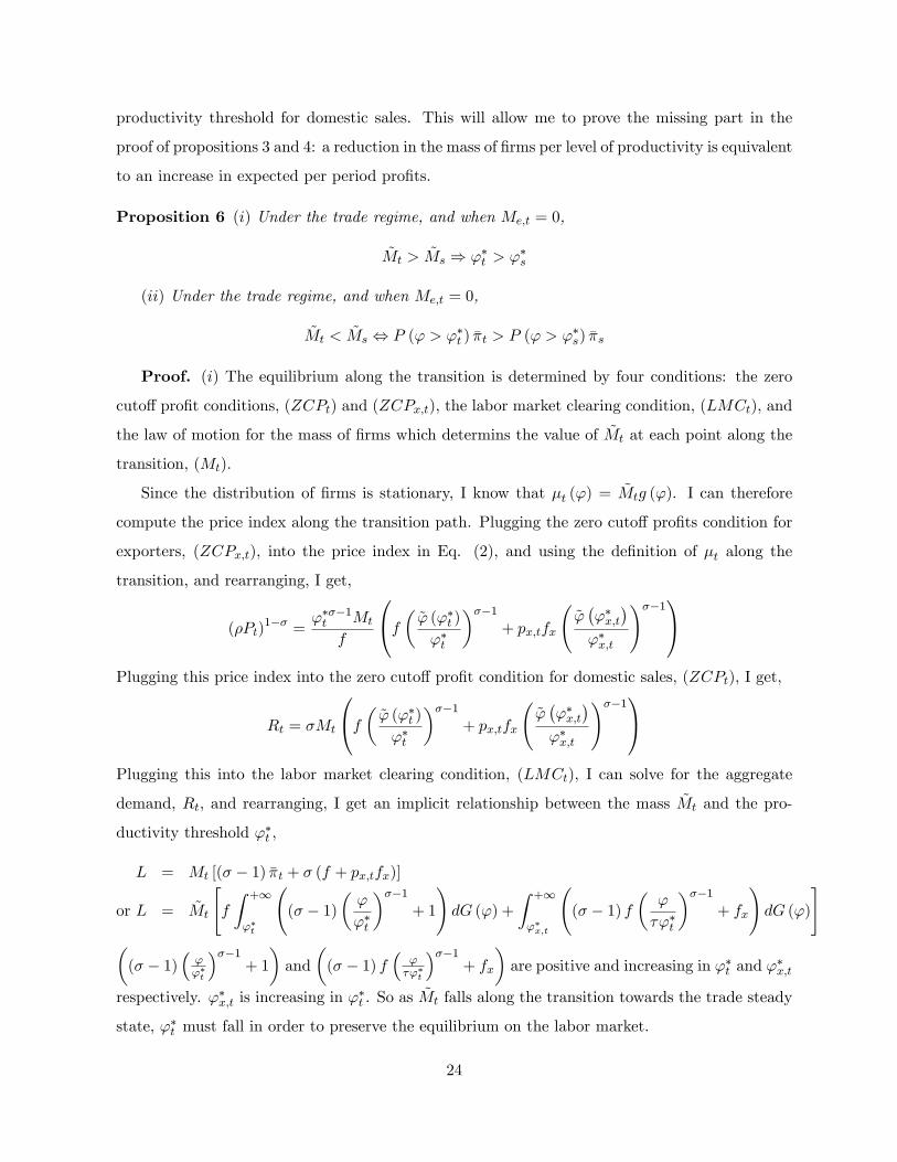
productivity threshold for domestic sales. This will allow me to prove the missing part in the

proof of propositions 3 and 4: a reduction in the mass of �rms per level of productivity is equivalent

to an increase in expected per period pro�ts.

Proposition 6 (i) Under the trade regime, and when Me;t = 0,

~Mt > ~Ms ) '�t > '�s

(ii) Under the trade regime, and when Me;t = 0,

~Mt < ~Ms , P (' > '�t ) ��t > P (' > '�s) ��s

Proof. (i) The equilibrium along the transition is determined by four conditions: the zero

cuto¤ pro�t conditions, (ZCPt) and (ZCPx;t), the labor market clearing condition, (LMCt), and

the law of motion for the mass of �rms which determins the value of ~Mt at each point along the

transition, (Mt).

Since the distribution of �rms is stationary, I know that �t (') = ~Mtg ('). I can therefore

compute the price index along the transition path. Plugging the zero cuto¤ pro�ts condition for

exporters, (ZCPx;t), into the price index in Eq. (2), and using the de�nition of �t along the

transition, and rearranging, I get,

(�Pt)1�� =

'���1t Mt

f

0@f � ~' ('�t )'�t

���1+ px;tfx

~'�'�x;t

�'�x;t

!��11APlugging this price index into the zero cuto¤ pro�t condition for domestic sales, (ZCPt), I get,

Rt = �Mt

0@f � ~' ('�t )'�t

���1+ px;tfx

~'�'�x;t

�'�x;t

!��11APlugging this into the labor market clearing condition, (LMCt), I can solve for the aggregate

demand, Rt, and rearranging, I get an implicit relationship between the mass ~Mt and the pro-

ductivity threshold '�t ,

L = Mt [(� � 1) ��t + � (f + px;tfx)]

or L = ~Mt

"f

Z +1

'�t

(� � 1)

�'

'�t

���1+ 1

!dG (') +

Z +1

'�x;t

(� � 1) f

�'

�'�t

���1+ fx

!dG (')

#�(� � 1)

�''�t

���1+ 1

�and

�(� � 1) f

�'�'�t

���1+ fx

�are positive and increasing in '�t and '

�x;t

respectively. '�x;t is increasing in '�t . So as ~Mt falls along the transition towards the trade steady

state, '�t must fall in order to preserve the equilibrium on the labor market.

24

So I have proven that along the transition, '�t increases as the mass of �rms ~Mt falls.

(ii) I will now prove that as '�t increases, P (' > '�t ) ��t decreases.

Plugging the zero cuto¤ pro�t conditions (ZCPt) and (ZCPx;t) into the formula for average

pro�ts, I get:

��t = f

�~'t'�t

���11

!+ px;tfx

0@ ~'x;t'�x;t

!��1� 1

1AMultiplying by the probability of survival, I get,

P (' > '�t ) ��t = f

Z +1

'�t

"�'

'�t

���1� 1#dG (') + fx

Z +1

'�x;t

24 '

'�x;t

!��1� 1

35 dG (')Since

��''�t

���1� 1�and

��''�x;t

���1� 1�are non negative and decreasing in '�t and '

�x;t respec-

tively, and since '�x;t is increasing in '�t , P (' > '

�t ) ��t is decreasing in '

�t .

C Expected opening to trade

If the opening to trade is announced in advance, productivity overshooting will be dampened.

Indeed, the very reason why there is overshooting in productivity is because the economy has

overaccumulated capital while in autarky, in the sense that too many �rms have been started.

The number of �rms must go down to its steady state level, and the absence of entry during

the transition explains why some less productive �rms have to temporarily stop their production,

and therefore why aggregate productivity overshoots in the short run. If the opening to trade is

expected, the economy will start disinveting in advance. Fewer �rms are created each period, so

that new �rms are not su¢ cient to replace exit each period. There is net exit of �rms even before

trade is opened up. This is because rational expectation agents do know that their investment

(creation of a new �rm) would not be worthwhile at least for some time. The speed at which

the economy disinvests obviously depends on the rate at which existing �rms die (the coe¢ cient

�), the impatience of entrepreneurs (the discount factor �), as well as the horizon at which trade

will be opened up. However, unless trade opening has been su¢ ciently early, there will still be

a period of productivity overshooting. There are too many of those �rms that had been created

before trade opening were announced, and those �rms will have to disappear.

We do observe that even those trade agreements that have been have been negotiated long in

advance, still have a large impact at the time when they are implemented.

25