Limited Participation and Consumption-Saving Puzzles:A Simple Explanation

Hong Liu and Guofu Zhou∗

This version: April, 2006(currently under revision)

∗Both authors are from Washington University in St Louis. Hong Liu, (314) 935–5883,liuh@wustl.edu; Guofu Zhou, (314) 935–6384, zhou@wustl.edu. We thank Jian Cai, John Campbell,Phil Dybvig, Michael Faulkender, Cam Harvey, Juhani Linnainmaa, Mark Loewenstein, Costis Ski-adas, Rong Wang, Kangzhen Xie, and seminar participants at Washington University in St. Louisfor helpful comments.

1

Limited Participation and Consumption-Saving Puzzles:

A Simple Explanation

Abstract

In this paper, we show that the existence of a large negative wealth shock and

the lack of insurance against such a shock can potentially explain both the limited

stock market participation puzzle and the consumption-saving puzzle that are widely

documented in the literature. This result holds for a general class of investor prefer-

ences and stock market characteristics, no matter how unlikely such a wealth shock is.

This explanation for limited participation does not require nonstandard preferences,

or transaction costs, or positive income beta with short-sale constraints, nor does it

require income growth or demographic structure shifting to explain low consumption

and high saving. We show that the availability of insurance can dramatically increase

stock market participation and current consumption and significantly decrease saving.

Journal of Economic Literature Classification Numbers: D11, D91, G11, C61.

Keywords: Limited participation, Insurance, Saving, Consumption

1. Introduction

As Campbell states in his 2006 presidential address: “Textbook financial theory im-

plies that all households, no matter how risk averse, should hold some equities if the

equity premium is positive.” However, less than 50% households in the U.S. partic-

ipate in the stock market and far less in many other countries (Mankiw and Zeldes

(1991), Haliassos and Bertaut (1995), Heaton and Lucas (2000), Guiso, Haliassos,

and Jappelli, 2003). As shown by Basak and Cuoco (1998), Cao, Hirshleifer and

Zhang (2005), and Huang and Wang (2006), limited participation has significant

impact on equilibrium risk premium, diversification discount, liquidity, and market

crashes. Several explanations have been proposed for this limited participation puz-

zle. Dow and Werlang (1992), Ang, Bekaert, and Liu (2005), Epstein and Schnei-

der (2005), and Cao, Wang, and Zhang (2005) show that nonparticipation can be

optimal if an investor has nonstandard preferences such as ambiguity or disappoint-

ment aversion. There are only few explanations based on traditional rational models.

Vissing-Jrgensen (2002) suggests that the decision to not invest in the stock market

can be optimal for about half of the non-participating individuals if they face modest

transactions costs. Cochrane (2005) challenges this explanation by pointing out that

“people who do not invest at all choose not to do so in the face of trivial fixed costs.”

Linnainmaa (2005) shows that the combination of learning and short-sale constraints

can generate non-participation for those investors whose income has a positive cor-

relation with the stock market. Consistent with these models, Campbell concludes

in his presidential address that “Thus to explain limited participation in the equity

market, we need either nonstandard preferences or fixed costs, which may be either

one-time-only entry costs or ongoing participation costs.”

There is also a growing literature on the low consumption-high-saving puzzle in

1

developing countries (e.g., Cao and Modigliani (2004)). For example, China’s per

capita income ranks below 100th in the world, but its saving rate has been among

the highest worldwide in recent decades. Cao and Modigliani (2004) offers an expla-

nation based on income growth, demographic structure, and inflation. It becomes

an important and challenging goal for these countries to lower saving and increase

consumption.

The first contribution of this paper is to provide a new rational explanation of

limited participation puzzle and the low-consumption-high-saving puzzle. In contrast

to the existing literature, our explanation of the limited participation puzzle does not

require nonstandard preferences, or fixed costs, or positive income beta with short-

sale constraints, nor does it require income growth or demographic structure shifting

to justify the low consumption and high saving. Specifically, in a simple two-period

consumption, saving, and investment model, we show that if a negative wealth shock

state, where the investor needs all of his current wealth to finance his subsistence

level consumption, exists with a positive (but possibly very small) probability, then a

rational investor does not participate in the stock market at all. This result holds for

general standard preferences, general stock market characteristics, and general wealth

processes. The large negative wealth shock may be due to bad health shocks such

as long term disability, diagnosis of severe diseases, unemployment risk, or bequest

requirement in the event of death. The basic intuition behind this main result is

that the investor has to save almost all of his initial wealth to hedge against this

negative wealth shock. He will not buy any stocks for the fear that their value may

go down when the wealth shock occurs. He will not short any stocks either, because

stock prices may go up when the negative shock happens. As a result, he will not

participate in the stock market at all, even if the risk premium is high. More generally,

2

our model suggests that in the presence of such a negative wealth shock, investors

will invest significantly less than what is predicted by a model that ignores such a

negative wealth shock and thus can also potentially help explain the equity premium

puzzle.

In addition, with this threat of negative wealth shock, current consumption will

be minimum and the investor will save almost all of his current wealth for the fu-

ture. This is because the investor needs almost all of his current wealth to absorb the

negative wealth shock and to maintain the subsistence level consumption if such a

shock occurs. Our model can thus help explain the low-consumption-high-saving puz-

zle widely documented for developing countries such as China, where large negative

wealth shocks are especially likely.

The second contribution is to propose insurance development as a solution to

the limited participation puzzle and the low-consumption-high-saving puzzle. The

role of insurance does not seem to have received much attention in the asset pricing

literature. Our model suggests that insurance coverage has a profound impact on

an investor’s portfolio decisions. In particular, we show that if there is an insur-

ance market for hedging the wealth shock, an investor may participate much more

in the stock market, consume much more, and save much less. Intuitively, when the

probability of the negative wealth shock is small, buying insurance is typically inex-

pensive. Since insurance provides an effective hedge against this shock, the investor

can afford to increase current consumption, invest more, and save less. Our numerical

analysis suggests that in some cases, he may even consume almost all of his current

wealth and save virtually nothing if his normal future wealth is high. Therefore, the

availability of insurance can dramatically change an investor’s consumption, saving,

and investment decisions. Our model suggests that insurance coverage is critical for

3

understanding household finance and thus asset pricing in general. Consistent with

this prediction, Qiu (2006) finds that, controlling for other relevant factors, “insured

households are more likely to own stocks and to invest a larger proportion of their

financial assets in stocks than uninsured households do.” In addition, Goldman and

Maestas (2005) find that better health insurance coverage is associated with greater

risky asset investment, while Chen et al. (2005) examine the joint determination of

life insurance and asset allocation.

Our model suggests that the low consumption and high saving phenomenon ob-

served in countries like China can be caused by the presence of significant negative

wealth shocks and the lack of insurance against these shocks. On the other hand,

the high consumption and low saving in countries like the U.S. may be due to the

much greater availability of various insurance programs.1 Our explanation for the low

saving rate in the U.S. thus compliments that of Shiller (2004) who attributes it to

the wealth effect of rising housing prices.

Our model is closely related to the extensive literature on precautionary saving

against background risk. For example, Kimball (1993) demonstrates that with the

standard risk aversion, in the presence of the zero-mean background risk, an investor

will invest less in the risky asset and save more. Koo (1991) and Guiso, Jappelli and

Terlizzese (1996) show that as the background risk of income increases, an investor

decreases risky asset investment. Our model seems to be the first to link background

risk to limited participation and the first to recognize a potential large negative wealth

shock as an important background risk for portfolio choice and asset pricing in ad-

dition to consumption and saving. Our model shows that no matter how small this

background risk is (in the sense that the probability of such a negative wealth shock

1The saving rate in the U.S. is less than 3%, which arguably drops below zero recently. See, e.g.,U.S. Economic Accounts, US Department of Commerce, Feb., 2006

4

can be arbitrarily small), it can prevent an investor from investing any amount of

cash into risky assets.

The rest of the paper is organized as follows. We describe the model in Section

2. Insurance market is then introduced in Section 3. We then present a graphical

illustration of a case with constant relative risk aversion preference (CRRA) in Section

4. Conclusions are offered in the final Section 5. Proofs are provided in the Appendix.

2. The Model

For simplicity, we consider a two-period model. An investor derives utility from

intertemporal consumption (c0, c1), which represents respectively consumption today

and consumption next period. The investor has an initial wealth of W0. His wealth

endowment next period will be W̃1, where with a possibly small probability ε > 0,

W̃1 = −D, which represents a negative wealth shock, and with probability 1 − ε,

W̃1 = W ≥ 0, which represents normal future wealth and may be interpreted as the

present value of labor income.

At the beginning of the period, the investor can consume, save, or invest in an risky

asset (stock). The initial stock price S0 is normalized to 1 and the next period stock

price is S̃1, where S̃1 = u > 1 with probability p, and S̃1 = d < 1 with probability

1 − p. We assume that the stock process is independent of the investor’s income

process.2 For simplicity, we assume further that the interest rate is zero.3 Then the

investor’s problem is to choose consumption c0, saving α, and stock investment θ to

2A minor modification of our main arguments applies to the case where these two processes arecorrelated.

3A nonzero interest rate would not change our main results.

5

solve

maxc0,α,θ

U(c0) + δE[U(c1)], (1)

subject to the budget constraints

α = W0 − c0 − θ, (2)

c0 = α + θS̃1 + W̃1, (3)

where

U(c) =

{u(c) if c ≥ c,

−∞ otherwise,(4)

where u(c) is strictly increasing and strictly concave for c ≥ c.4 δ is the subjective

time discount rate and c is the subsistence level of consumption.

In the above standard set-up, we make the following nonstandard assumption:

Assumption A The magnitude of the negative wealth shock

D = W0 − 2c > 0. (5)

This is the key assumption of this paper.5 Under this assumption, with a positive,

but possibly arbitrarily small, probability ε, the investor will need all his initial wealth

to maintain the subsistence level of consumptions in both periods. There are several

reasons why a shock of this magnitude may occur. Let us focus the case of the

4Following the usual convention, we assume that if u(c) = −∞, then the investor would stillchoose to prevent consumption from falling below c, even though he is indifferent at c. This ispurely for expositional simplicity, since a slight modification of the preference would suffice to avoidthis indifference.

5Assuming D takes exactly one value is for simplicity. The main results still obtain even whenthere are many states with different levels of wealth shocks as long as one of them is of the magnitudeof W0 − 2c.

6

U.S. investors. According to year 2000 census, the median net worth in the U.S.

is $55,000, and $13,473 if excluding home equity.6 This level of wealth is clearly

not nearly enough to finance large and unanticipated expenses. There are several

scenarios in which such large and unanticipated expenses may arise. First, it may

occur due to severe health shocks. For example, sudden long term disability and a

diagnosis of a terminal condition may require large expenses that can far exceed the

existing wealth level of an investor. If the investor has health insurance, the problem

may be less severe, but certainly not eliminated. The fact that there are over 45

million Americans who had no health insurance in 20047 certainly makes the problem

an important issue as they represent about one quarter of the population.

Second, an investor may desire to leave a bequest to his family if he deceases next

period. The probability for such an event is clearly positive, and the desired bequest

level often exceeds what the investor has. In practice, this high level of bequest is often

achieved through life insurance. While we do not have the participation rate for life

insurance, it will unlikely be higher than the participation rate for health insurance.

Third, unemployment risk is significant and can be devastating to the working class.

In the event of unemployment, the unemployed needs a large sum of wealth to main-

tain a minimum standard of living for the uncertain duration of unemployment. The

required wealth can also far exceed his current wealth. For example, Gruber (2002)

provides evidence that using their current wealth, “almost one-third of workers cant

even replace 10% of their income loss” due to unemployment. In short, the assump-

tion of a large negative wealth shock, with possibly tiny but nonzero probability, is a

6Source: Table B and Figure 7 of Net Worth and Asset Ownership of Households: 1998 and2000, an publication issued by the U.S. Census Bureau in 2003.

7See, e.g., Kaiser Commission On Medicaid And The Uninsured, a 2006 publication of the KaiserFamily Foundation.

7

realistic constraint on typical household investment decisions.8

On the optimal portfolio choice, we have

Proposition 1 Under Assumption A, the investor does not participate in the stock

market, i.e., θ∗ = 0. In addition, the investor only consumes the minimum and saves

the rest, i.e., c∗0 = c and α∗ = W0 − c.

Proof. See Appendix.

Proposition 1 says that, in the presence of the wealth shock state, the investor will

not participate in the stock market at all. This result depends neither on the proba-

bility of the negative wealth shock state (as long as it is positive), nor the magnitude

of the stock risk premium. Intuitively, longing or shorting in the stock always involves

risk. Since any loss in the stock investment would incur an infinite utility loss if the

bad wealth shock occurs, the investor optimally chooses not to participate in the stock

market today. This result holds for a general class of preferences, wealth profiles, and

stock market characteristics. In contrast to the existing studies such as Dow and

Werlang (1992), Ang, Bekaert, and Liu (2005), Epstein and Schneider (2005), Cao,

Wang, and Zhang (2005), Vissing-Jrgensen (2002) and Linnainmaa (2005), we do not

need any behavioral assumptions or any market frictions such as transaction costs or

short-sale constraints or any labor income correlation with the stock market to justify

the stock market nonparticipation.

Proposition 1 also shows that the presence of the negative wealth shock state, no

matter how small the likelihood is, can cause extremely low current consumption and

8Even for investors in the upper percentiles of the wealth distribution, the existence of such anegative wealth shock, though might not be as bad as in Assumption A, can still significantly reducetheir stock investment. Although beyond the scope of this paper, this is likely to reduce the tradingcosts required for non-participation in the Vissing-Jrgensen (2002) model.

8

extremely high saving. In particular, the investor will only consume the minimum

amount of the subsistence level today and save the rest of his wealth to hedge against

the possible bad wealth shock in the future.

It is worth noting that the nonparticipation and an extremely high saving rate

arise no matter how high the investor’s wealth in other states is. This implies that

as long as the wealth shock in one state of the world is bad enough, even the wealthy

people will not participate in the stock market and saves almost all of his wealth for

the future. This prediction is consistent with the empirical finding that even wealthy

people have a low participation rate in the stock market (Heaton and Lucas (1997)).

3. Consumption, saving, and investment with in-

surance coverage

A natural and important question is then how a country like China can increase stock

market participation, increase current consumption, and decrease saving, in order

to achieve sustained economic growth. In this section, we offer a simple solution:

Develop insurance industry.9

Suppose now that the investor can purchase an insurance against the negative

wealth shock state and the insurance premium per dollar coverage is equal to λ. Let

I be the dollar amount the investor chooses to insure. Since most insurance programs

are compensatory in the sense that insurance claim payment usually does not exceed

9Empirically, “there is a positive correlation between a country’s level of development and insur-ance coverage.” (See p. 7 of Trade and Development Aspects of Insurance Services and RegulatoryFramework, United Nations Publications, 2005)

9

the full coverage of an damage, we assume that the investor cannot overinsure, i.e.,

I ≤ D. (6)

Then the investor solves:

maxc0,s,θ,I

U(c0) + δE[U(c1)],

subject to the budget constraints

α = w − c0 − θ − λI, (7)

c0 = α + θS̃1 + W̃1 + I1{W1=−D}, (8)

and (6).

In contrast to Problem (1), the investor now can hedge against the negative wealth

shock state using insurance. For simplicity, we assume in what follows that the

insurance premium is fair, i.e., λ = ε.10 Then, on the investor’s optimal level of

insurance, we have

Proposition 2 Suppose λ = ε. Then there exists a ε > 0 such that ∀ ε < ε, full

insurance is optimal, i.e., I∗ = D.

Proof. See Appendix.

The intuition for the proposition is that if the cost of insurance per dollar coverage

is not too high, the investor will pay the small cost of insurance to protect fully

against the wealth shock, irrespective of his wealth level and risk aversion. Because

of the high demand for insurance, there are social welfare gains for making insurance

10The results will not alter qualitatively as long as the premium rate is not too unfair.

10

products available in the economy. Note that there are two channels to ensure that

the investor’s consumption level next period, c1, will be above the subsistence level

c. The first is saving and the second is insurance. When the insurance is relatively

inexpensive (e.g., ε and thus λ are small), the investor buys full coverage to ensure

the subsistent level consumption c even without saving. Saving is an inefficient way

of hedging, especially when the wealth shock state is a small probability event and

normal future wealth is high (i.e., W − 1 is large). This is because saving reduces

current consumption and can transfer it to states where marginal utility consumption

is low (i.e. wealth is high). In contrast, insurance transfers current consumption only

to the states where marginal utility of consumption is high. The tradeoff between

saving and insurance in general will be examined in the next section.

On stock market participation, we have

Proposition 3 If the insurance is available and if the stock has nonzero risk pre-

mium, we have θ∗ 6= 0.

Proof. See Appendix.

This proposition suggests that with insurance, as long as the risk premium is

nonzero, an investor will optimally participate in the stock market, no matter how

poor he is. This result suggests that developing an insurance market can potentially

help raise the stock market participation and lower the risk premium. In practice,

the insurance coverage and costs vary. The implication of the proposition is that

participation rate in the stock market depends on the participation rate in the in-

surance markets. Our model thus predicts that participation rate in the insurance

markets is positively correlated to that in the stock market. This prediction is con-

sistent with the recent empirical findings of Qiu (2006). In particular, Qiu (2006)

11

finds that insured households ar more likely to own stocks and they tend to invest

a larger proportion of their financial assets in stocks than uninsured households do.

Our model provides an explanation of his finding. Our model suggests that the in-

teractions among insurance, consumption, saving, and portfolio choice can be a new

line of promising research.

With insurance, we expect that the investor will increase his current consumption

since he no longer has to save a lot to protect himself against the bad wealth shock.

Indeed, the following proposition confirms this intuition.

Proposition 4 ∀ c ≤ c0 < W0 − c, there exist W̄ , ε such that ∀W > W̄, ε < ε, we

have c∗0 > c0.

Proof. See Appendix.

This proposition says that if the investor’s future wealth is high enough and the

probability of bad wealth shock is low enough, then the investor will consume almost

all of his initial wealth. So the saving rate would dramatically drop and consump-

tion would significantly rise in the presence of insurance. Many developing countries

face high saving rate and low consumption problems. They adopt various policies

attempting to stimulate consumption and lower saving rate. For example, the Chi-

nese government in recent years lowered its interest rates substantially to dissuade

people from saving. Our model suggests that without insurance, no matter how low

the interest rates are, an investor will save almost all of his wealth for the protection

against the possible bad wealth shock in the future. With insurance, however, the

investor will consume much more and save much less than otherwise, if the probability

of large negative wealth shock is small.

The analysis above also suggests an important policy implication from our model:

12

developing countries may better achieve their goal of deceasing saving rate and in-

creasing consumption by developing their insurance industry. While it is difficult to

analyze the relation between savings and insurance in developing countries due to lack

of data, it is interesting to examine whether there exists a positive relation between

them for the developed countries. For 13 OECD countries where the annual data is

consistently available from 1994 to 2003,11 we run a simple regression of the saving

rates measured as the percent of household savings to disposal household income on

insurance penetration measured as the percent of premiums to GDP. Table 1 reports

the results. The betas, slopes of the regression, are all negative except Denmark

which has a insignificant positive value of 1.56. The adjusted R2 are high for most

of the countries. The results seem to suggest strongly that, as insurance industries

develop in each country, the saving rates decrease overtime, as our model implies.

4. Numerical Analysis

In this section, to obtain further insights, we solve numerically an example where

an investor has a CRRA preference and graphically illustrate the implications of our

model. The CRRA utility function is:

U(c) =

{c1−γ

1−γif c > 0,

−∞ otherwise,

In our analysis below, we use the following default parameter specification: γ = 2,

p = 0.999, ε = 0.1%, u = 2, d = 0, W0 = 1, W1 = 2, D = W0, and λ = ε. A brief

discussion of some of the default parameter value is in order. We set ε to be low so

that the negative wealth shock is a small probability event. We set p to be high to

11Source: OECD Statistics Books, OECD Publications, 2005.

13

Table 1: Savings and Insurance

The table reports the slope, its t-statistic and the adjusted R2 of the regression ofsaving rates measured as the percent of household savings to its disposal income oninsurance penetration measured as the percent of premiums to GDP,

Savingst = ι + β × Insurancet + εt, t = 1, . . . , T,

where T = 10 is the available sample size. The data is annual from 1994 to 2003.

Country β t-statistic Adjusted R2

Austria -1.96 (-1.35) 0.19Belgium -1.49 (-6.01) 0.82Canada -0.95 (-2.56) 0.45Denmark 1.56 (1.81) 0.29Finland -2.22 (-3.04) 0.54France -0.06 (-0.14) 0.00Germany -0.50 (-1.38) 0.19Italy -2.28 (-5.15) 0.77Netherlands -2.68 (-3.57) 0.61Spain -6.81 (-3.57) 0.62Switzerland -0.58 (-0.62) 0.05United Kingdom -0.87 (-6.28) 0.83United States -0.11 (-0.24) 0.01

14

emphasize the fact that even a small downside risk in the stock market may deter

participation, in the absence of insurance. We set the normal future wealth W1 to

be 2 to illustrate that high norma wealth does not change our main results. We pick

u = 2 to show that high risk premium does not change our main results either (recall

that the interest rate is set to be 0 for simplicity).

It is interesting, as shown by Figure 1, that with low enough insurance coverage,

the investor will almost invest nothing in the stock market.12 After the coverage in-

creases to a threshold, the participation starts to rise sharply. However, if the investor

can insure more than the full coverage, then stock investment starts to decline. This

is because with the overinsurance, the marginal utility of consumption in the bad

wealth shock state decreases and the investor starts to decrease his stock investment

to increase his current consumption.

Figures 2 and 3 show that as insurance coverage increases the consumption rate

increases and the saving rate decreases. When the investor is fully insured, he con-

sumes almost all of his initial wealth and saves nothing. In addition, Figure 3 shows

that saving rate is largely determined by the insurance coverage. When the investor

is underinsured, he saves enough to make up the difference. These findings suggest

that insurance may be critical and effective for increasing consumption and decreas-

ing saving. These three figures also show that a higher probability of the negative

wealth shock leads to a lower stock investment, a lower consumption rate, and a

higher saving rate, as expected.

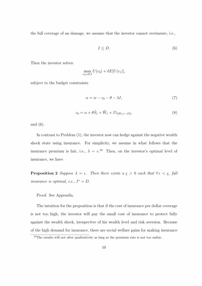
In the standard portfolio choice models, as risk aversion increases, the fraction

of wealth invested in stock decreases (e.g., Merton (1971), Cochrane (2001), Liu and

Loewenstein (2002), Liu (2004)). Interestingly, as Figure 4 shows that while this is

12In this analysis, we allow the investor to overinsure to examine the effect of overinsurance.

15

0.2 0.4 0.6 0.8 1 1.2 1.4

0.025

0.05

0.075

0.1

0.125

0.15

Insurance Coverage

I

e=0.1%

e=1%

Fraction of wealth in stock

Figure 1: The fraction of wealth invested in the stock against insurancecoverage available for parameters: p = 0.999, W1 = 2, u = 2, d = 0, W0 = 1,D = W0, and λ = ε.

0.2 0.4 0.6 0.8 1 1.2 1.4

0.2

0.4

0.6

0.8

1

Insurance Coverage

I

Consumption Rate

e=0.1%

e=1%

Figure 2: The consumption rate against insurance coverage available forparameters: p = 0.999, W1 = 2, u = 2, d = 0, W0 = 1, D = W0, and λ = ε.

16

0.2 0.4 0.6 0.8 1 1.2 1.4

0.2

0.4

0.6

0.8

Insurance Coverage

I

Saving Rate

e=1%

e=0.1%

Figure 3: The saving rate against insurance coverage available for param-eters: p = 0.999, W1 = 2, u = 2, d = 0, W0 = 1, D = W0, and λ = ε.

true for those who have low normal future wealth (i.e., W1 is small), it is in general

incorrect for those who have a high normal future wealth. In particular, for those who

have very high normal future wealth (W1 = 4), the opposite is true. Intuitively, the

investor faces two types of risks: Stock investment losses and bad wealth shocks. Risk

aversion coefficient thus has two opposite effects on the stock investment. On the one

hand, the investor has tendency to invest more in the stock as risk aversion decreases.

However, this would imply a decrease in the current consumption (recall that saving

rate is largely determined by insurance coverage). On the other hand, as the risk

aversion decreases, the investor is less concerned about the bad wealth shock, and

thus would like to consume more today. This tends to decrease the stock investment

today. The net effect depends on the relative marginal utility of consumption today

and tomorrow and the magnitude of the risk aversion. When the normal future

wealth is high, the marginal utility of consumption tomorrow is relatively small, and

therefore, as risk aversion decreases, the investor decreases his investment to increase

consumption, as shown in Figure 5.

17

1 2 3 4 5

0.1

0.2

0.3

0.4

0.5

0.6

Fraction of wealth in stock

Risk Aversion

g

W1=0

W1=2

W1=4

Figure 4: The fraction of wealth invested in the stock against risk aversionfor parameters: p = 0.999, ε = 0.1%, u = 2, d = 0, W0 = 1, D = W0, and λ = ε.

Figure 6 shows that, as the risk aversion coefficient increases, the investor saves

more. Intuitively, as risk aversion increases, the investor becomes more concerned

about both stock investment losses and bad wealth shock and therefore invests and

consumes less today and saves more for the future.

Figure 7 shows how the stock investment changes with normal future wealth W1.

It shows that as the investor’s normal future wealth increases, he invests less in stock

today. This drop in the stock investment is due to the decrease of the marginal utility

of future consumption, which makes the current consumption more valuable, and thus

the investor invests less in order to consume more today, as shown in Figure 8. Figure

9 shows that the saving rate stays almost constant. As we show before in Figure 3,

saving rate is largely determined by insurance coverage. As before, lower coverage

lowers stock investment, consumption, and increases saving rate.

18

1 2 3 4 5 0.3

0.4

0.5

0.6

0.7

0.8

0.9

1

Consumption Rate

Risk Aversion

W1=0

W1 =4

W1

=2

g

Figure 5: The fraction of wealth consumed against risk aversion for pa-rameters: p = 0.999, ε = 0.1%, u = 2, d = 0, W0 = 1, D = W0, and λ = ε.

1 2 3 4 5

0.05

0.1

0.15

0.2

W1=0

W1=2

W1=4

Risk Aversion

g

Saving Rate

Figure 6: The saving rate as a fraction of current wealth against riskaversion for parameters: p = 0.999, ε = 0.1%, u = 2, d = 0, W0 = 1, D = W0,and λ = ε.

19

0.5 1 1.5 2

0.05

0.1

0.15

0.2

0.25

0.3

Future normal wealth

W1

I=1

I=0.7

5

Fraction of wealth in stock

Figure 7: The fraction of wealth invested in the stock against normalfuture wealth for parameters: γ = 2, p = 0.999, ε = 0.1%, u = 2, d = 0,W0 = 1, D = W0, and λ = ε.

0.5 1 1.5 2

0.65

0.7

0.75

0.8

0.85

0.9

0.95

Future normal wealth

W1

Consumption Rate

I=0.75

I=1

Figure 8: The consumption rate against normal future wealth for param-eters: γ = 2, p = 0.999, ε = 0.1%, u = 2, d = 0, W0 = 1, D = W0, andλ = ε.

20

0.5 1 1.5 2

0.05

0.1

0.15

0.2

0.25

Future normal wealth

Saving Rate

I=1

I=0.75

W1

Figure 9: The saving rate as a fraction of current wealth against normalfuture wealth for parameters: p = 0.999, ε = 0.1%, u = 2, d = 0, W0 = 1,D = W0, and λ = ε.

5. Conclusions

We provide an alternative explanation of the limited stock market participation and

the low-consumption-high-saving puzzles: the existence of significant negative wealth

shock and the lack of sufficient insurance. We show that no matter how unlikely the

negative wealth shock is, in the absence of insurance, it is rational for investors to not

participate in the stock market at all, to consume a minimum amount, and to save

almost all of his wealth. However, once insurance is available at a reasonable cost, we

find that investors will in general participate more in the stock market, consume more,

and save less. Our model suggests that developing a better insurance industry can

be a solution to the limited participation, low consumption, and high saving issues in

countries like China.

There is little research devoted to insurance and asset pricing. Further theoretical

and empirical work are necessary for understanding how insurance affect investors’

21

life-cycle consumption, saving, and investment decisions.

22

Appendix

In this appendix, we provide all the proofs.

Proof of Proposition 1. The investor’s problem can be written as

maxc0,θ

U(c0) + δ[p(1− ε)U(W0 − c0 − θ + θu + W1)

+(1− p)(1− ε)U(W0 − c0 − θ + θd + W1)

+pεU(W0 − c0 − θ + θu−D)

+(1− p)εU(W0 − c0 − θ + θd−D)]. (9)

Suppose w > 0, then we have

W0 − c0 − θ + θd−D ≤ W0 − c0 − θ + θd− (W0 − 2c)

≤ c− θ + θd

< c.

So the fourth term in (9) is −∞ and other terms less than +∞. Therefore, we must

have α∗ ≤ 0. Similar argument on the third term leads to the conclusion that α∗ ≥ 0.

Thus we must have w∗ = 0. Given that α∗ = 0, and U(c) = −∞ for any c < c, we

must have c∗0 = c. ¤

Proof of Proposition 2. Taking the first derivative of the objective function

with respect to I, we have

δ[p(1− ε)εU ′(W0 − c0 − εI − θ + θu + W1) (10)

23

+(1− p)(1− ε)εU ′(W0 − c0 − εI − θ + θd + W1) (11)

+pε(1− ε)U ′(W0 − c0 − εI − θ + θu + I −D) (12)

+(1− p)(1− ε)εU ′(W0 − c0 − εI − θ + θd + I −D)], (13)

which is always greater than 0 because the third (fourth) term is always greater than

the first (second) term, due to the strict concavity of the utility function and I ≤ D.

In addition, I = D is feasible for small enough ε because Assumption A guarantees

that at ε = 0 “buying” full insurance is feasible. Therefore, we must have I∗ = D. ¤

Proof of Proposition 3. Taking the first derivative of the objective function

in (9) with respect to θ and evaluating it at ε = 0, we have

(p u + (1− p) d− 1)[U ′(W0 − c0 − λI + W1) + U ′(W0 − c0 − λI + I −D)],

which is always positive (negative) if (p u + (1 − p) d − 1) > (<)0 for any optimal

choice of c0 = c∗0 and I = I∗, since the utility function is strictly increasing. This

implies that θ∗ 6= 0 as long as the risk premium (p u+(1− p) d− 1) is not zero (recall

that we set interest rate to zero for notational simplicity). ¤

Proof of Proposition 4. As W1 approaches ∞ and ε approaches 0, the first

derivative of the objective function in (9) with respect to c0 approaches U ′(c0) > 0.

This implies that c∗0 must approach W0 and hence greater than any c̄ < W0. ¤

24

References

Basak, S., and D. Cuoco, 1998, An equilibrium model with restricted stock market

participation, Review of Financial Studies 11, 309–341.

Campbell, J. Y., 2006, Household finance, forthcoming, Journal of Finance.

Cao, H., T. Wang, and H. H. Zhang, 2005, Model uncertainty, limited market par-

ticipation, and asset prices, Review of Financial Studies 18, 1219–1251.

Cao, H., D. Hirshleifer and H. H. Zhang, 2005, Diversification and capital gains taxes

with multiple risky assets, Working Paper, Cheung Kong Graduate School of

Business.

Cao, S. L., and F. Modigliani, 2004, The Chinese saving puzzle and the life-cycle

hypothesis, Journal of Economic Literature 42, 145–170.

Chen, P., R. Ibbotson, M. Milevsky, and K. Zhu, 2005, Human capital, asset allo-

cation, and life insurance, forthcoming, Financial Analysts Journal.

Cochrane, J. H., 2001, Asset Pricing, Princeton University Press, NJ.

Cochrane, J. H., 2005, Financial markets and the real economy, Working Paper,

University of Chicago.

Dow, J., and S. Werlang, 1992, Uncertainty aversion, risk aversion and the optimal

choice of portfolio, Econometrica 60, 197–204.

Epstein, L., and M. Schneider, 2005, Learning under ambiguity, Working Paper,

University of Rochester.

25

Goldman, D. P., and N. Maestas, 2005, Medical expenditure risk and household

portfolio choice, Rand Working Paper.

Gruber, J., 2002, The wealth of the unemployed, Industrial and Labor Relations

Review 55, 79–94.

Guiso, L., M. Haliassos, and T. Jappelli, 2003, Household stockholding in Europe:

Where do we stand and where do we go? Economic Policy 18, 117–164.

Guiso, L., T. Jappelli and D. Terlizzese, 1996, Income risk, borrowing constraints

and portfolio choice, American Economic Review 86, 158–72.

Haliassos, M., and C. Bertaut, 1995, Why do so few hold stocks?, Economic Journal

105, 1110–1129.

Heaton, J., and D. Lucas, 1997, Market frictions, savings behavior and portfolio

choice, Macroeconomic Dynamics 1, 76–101.

Heaton, J., and D. Lucas, 2000, Portfolio choice and asset prices: The importance

of entrepreneurial risk, Journal of Finance 55, 1163–1198.

Huang, J., and J. Wang, 2006, Market liquidity and asset prices under costly par-

ticipation, Working Paper, MIT.

Kimball, M.S., 1993, Standard risk aversion, Econometrica 60, 589–611.

Koo, H.K., 1991, Consumption and portfolio choice with uninsured income risk,

Mimeo, Princeton University.

Linnainmaa, J., 2005, Learning and stock market participation, Working Paper,

UCLA.

26

Liu, H., 2004, Optimal consumption and investment with transaction costs and

multiple risky assets, Journal of Finance 59, 289–338.

Liu, H., and M. Loewenstein, 2002, Optimal portfolio selection with transaction

costs and finite horizons, Review of Financial Studies 15, 805–835.

Mankiw, N. G., and S. P. Zeldes, 1991, The consumption of stockholders and non-

stockholders, Journal of Financial Economics 29, 97–112.

Qiu, J. P., 2006, Precautionary saving and health insurance: A portfolio choice

perspective, Working Paper, Wilfrid Laurier University.

Shiller, R.J., 2004, Household reaction to changes in housing wealth, Working Paper,

Yale University.

Vissing-Jrgensen, A., 2002, Towards an explanation of household portfolio choice

heterogeneity: Nonfinancial income and participation cost structures, Working

Paper, NBER.

27