Embed Size (px)
Citation preview
Consumption, Saving, and Investment
Topic 3
1 Macroeconomics 309 - Lecture 3
Macroeconomics 309 - Lecture 32
Goals for Today’s Class – Start Modeling Aggregate Demand (AD)
What drives business investment decisions?
Does investment theory accurately match the data? What is the role of inventory?
What drives household consumption?
Does consumption theory accurately match the data? What theories of consumption seem to match the data? What role can the government play in shaping spending? Should a distinction be made between unexpected and expected changes and
permanent and temporary changes in income? What is the link between consumption and savings?
Macroeconomics 309 - Lecture 33
Part I: Investment
Macroeconomics 309 - Lecture 34
An Introduction to Investment
Second major component of spending
Includes purchase and construction of capital goods (fixed capital); inventories; residential structures.
Two reasons why studying investment is important:
1. It matters more for business cycle fluctuations. Much more volatile than consumption (accounts for 1/6 of GDP but more than ½ of decline in spending in a recession).
2. Determines long-run productive capacity of an economy (output is higher if capital stock is higher).
Macroeconomics 309 - Lecture 35
Desired Capital Stock
Firms optimize the amount of capital to have (just like they optimize the amount of labor to hire).
Remember from Topic 2: For the optimal amount of labor, firms equate the MPN with the real wage (cost of an additional unit of labor).
For the optimal amount of capital, firms equate the MPK (per period benefit of one more unit of capital) with the per period cost of an additional unit of capital.
How does capital evolve: Kt+1 = (1-δ) Kt + It
• i.e. Capital is increased tomorrow by investing today (less depreciation).• So the desired capital stock is determined by future MPK and expected user cost of
capital
What is the cost of an additional unit of capital (user cost of capital)?
Macroeconomics 309 - Lecture 36
User Cost of Capital
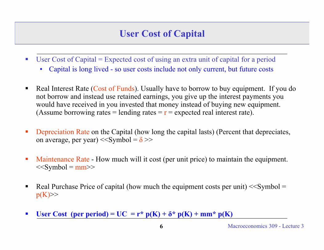
User Cost of Capital = Expected cost of using an extra unit of capital for a period• Capital is long lived - so user costs include not only current, but future costs
Real Interest Rate (Cost of Funds). Usually have to borrow to buy equipment. If you do not borrow and instead use retained earnings, you give up the interest payments you would have received in you invested that money instead of buying new equipment. (Assume borrowing rates = lending rates = r = expected real interest rate).
Depreciation Rate on the Capital (how long the capital lasts) (Percent that depreciates, on average, per year) <<Symbol = δ >>
Maintenance Rate - How much will it cost (per unit price) to maintain the equipment. <<Symbol = mm>>
Real Purchase Price of capital (how much the equipment costs per unit) <<Symbol = p(K)>>
User Cost (per period) = UC = r* p(K) + δ* p(K) + mm* p(K)
Macroeconomics 309 - Lecture 37
Desired Capital Stock (Cont.)
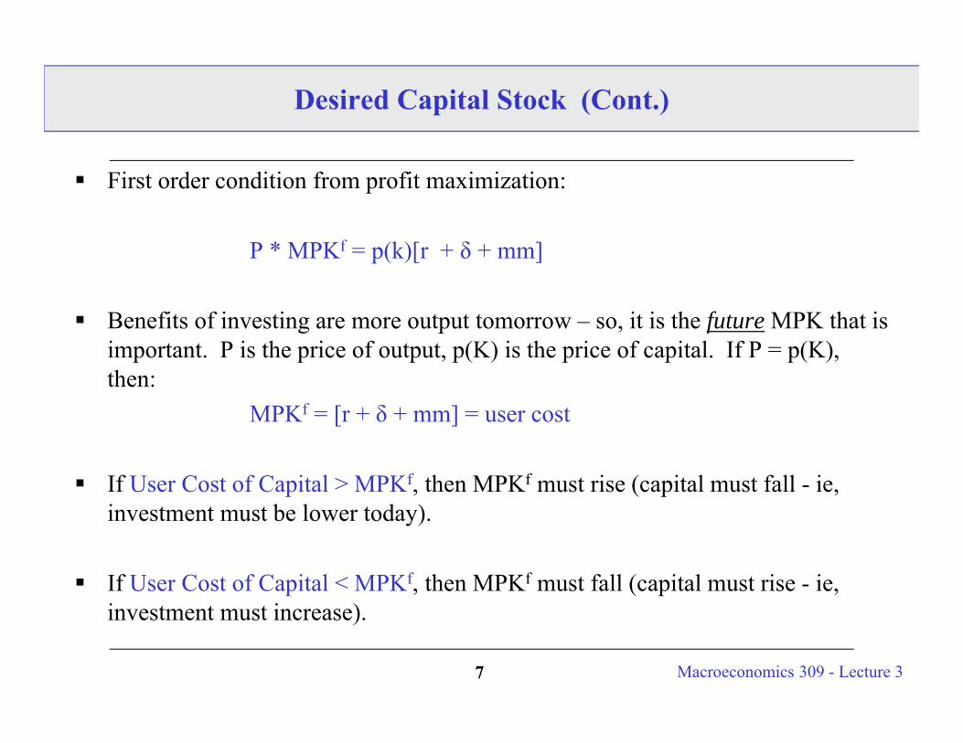
First order condition from profit maximization:
P * MPKf = p(k)[r + δ + mm]
Benefits of investing are more output tomorrow – so, it is the future MPK that is important. P is the price of output, p(K) is the price of capital. If P = p(K), then:
MPKf = [r + δ + mm] = user cost
If User Cost of Capital > MPKf, then MPKf must rise (capital must fall - ie, investment must be lower today).
If User Cost of Capital < MPKf, then MPKf must fall (capital must rise - ie, investment must increase).
Macroeconomics 309 - Lecture 38
The Desired Capital Stock
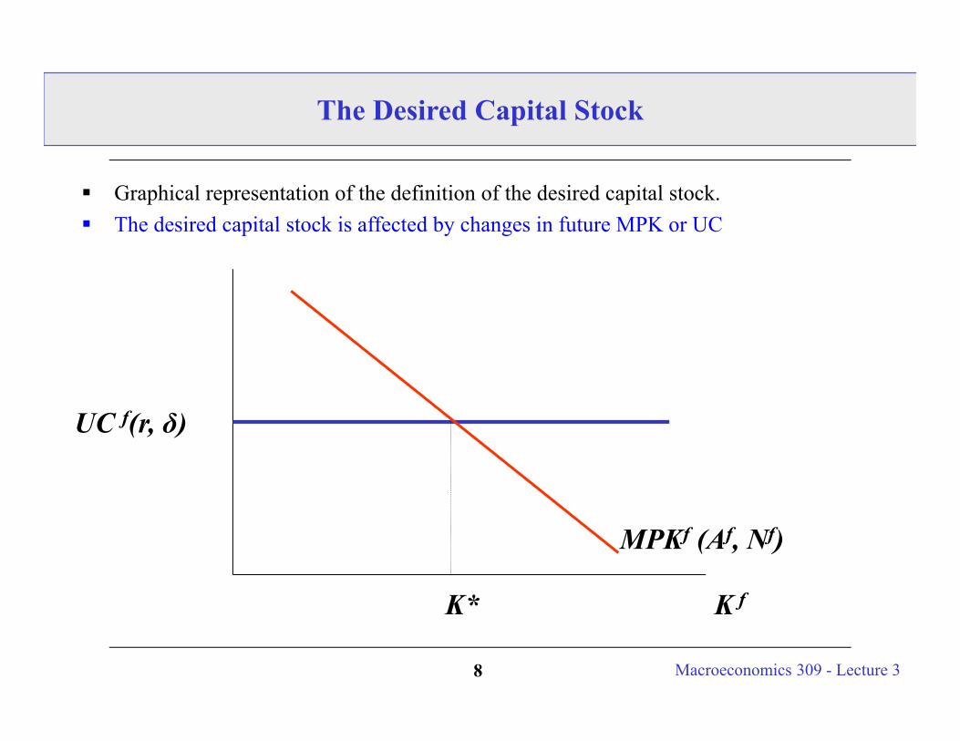
Graphical representation of the definition of the desired capital stock. The desired capital stock is affected by changes in future MPK or UC
UC f(r, δ)
MPKf (Af, Nf)
K fK*
Macroeconomics 309 - Lecture 39
Changes in the Desired Capital Stock: Af increases
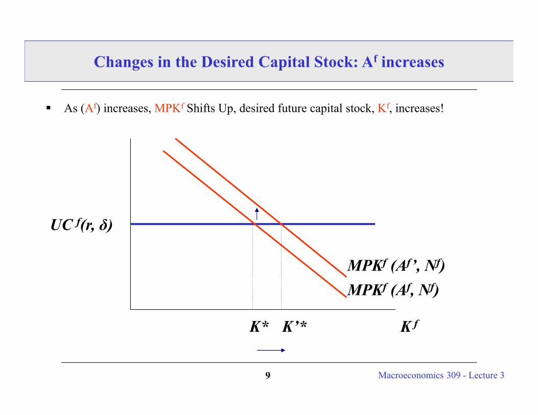
As (Af) increases, MPKf Shifts Up, desired future capital stock, Kf, increases!
UC f(r, δ)
MPKf (Af, Nf)
K fK* K’*
MPKf (Af’, Nf)
Macroeconomics 309 - Lecture 310
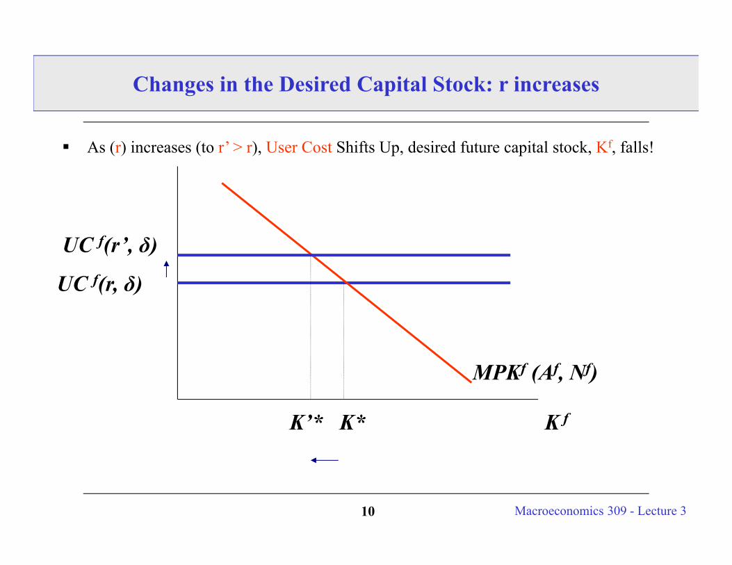
Changes in the Desired Capital Stock: r increases
As (r) increases (to r’ > r), User Cost Shifts Up, desired future capital stock, Kf, falls!
UC f(r, δ)
MPKf (Af, Nf)
K fK*
UC f(r’, δ)
K’*
Macroeconomics 33040 - Lecture 311
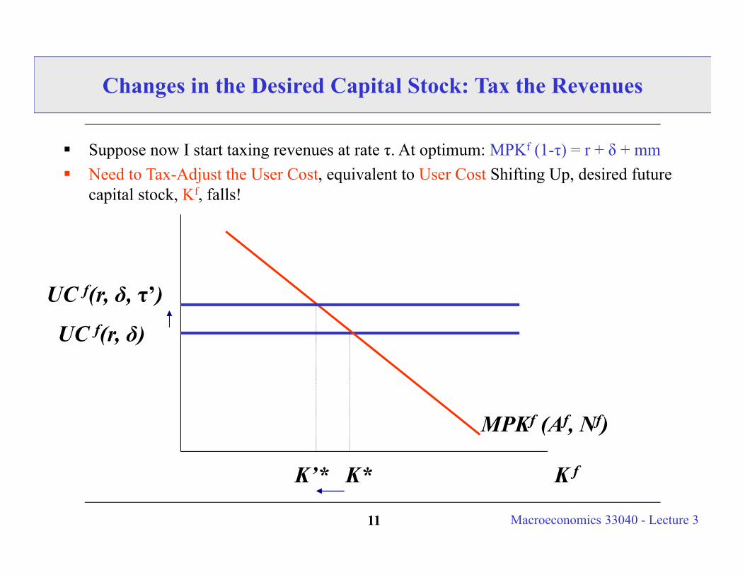
Changes in the Desired Capital Stock: Tax the Revenues
Suppose now I start taxing revenues at rate τ. At optimum: MPKf (1-τ) = r + δ + mm Need to Tax-Adjust the User Cost, equivalent to User Cost Shifting Up, desired future
capital stock, Kf, falls!
UC f(r, δ)
MPKf (Af, Nf)
K fK*
UC f(r, δ, τ’)
K’*
Macroeconomics 309 - Lecture 312
Reaching the Desired Capital Stock: Investment
Rationale: Investment decisions today have effects on the capital stock tomorrow. It takes time to build, install, train workers, etc. This is especially true with large expenditures (buildings, structures, assembly lines, etc).
Recall how capital evolves: Kt+1 = (1-δ) Kt + It
• i.e. Capital is increased tomorrow by investing today (less depreciation).• Gross investment is It; Depreciation is δKt; Net investment is Kt+1-Kt• Net Investment = Gross Investment - Depreciation
If K* is the desired capital stock then K* = (1-δ) Kt + It
A change in K* produces a change in It. The relationship is 1-to-1. Investment is the means to achieve the optimal capital stock.
Macroeconomics 309 - Lecture 313
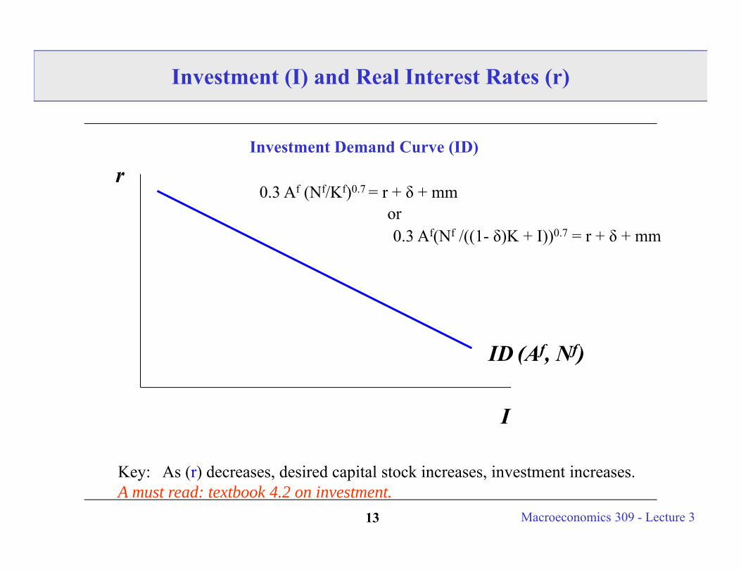
Investment (I) and Real Interest Rates (r)
Investment Demand Curve (ID)
ID (Af, Nf)
Key: As (r) decreases, desired capital stock increases, investment increases.A must read: textbook 4.2 on investment.
0.3 Af (Nf/Kf)0.7 = r + δ + mmor0.3 Af(Nf /((1- δ)K + I))0.7 = r + δ + mm
r
I
Macroeconomics 309 - Lecture 314
Investment: Some Caveats on the Process
Investment takes time to plan.
Investment tends to be ‘irreversible’ (costly to change if you over/under invest).
Investment returns are uncertain (returns are in the future - which is unknown).• As economic uncertainty increases, investment decisions can become delayed.
Firms - like individuals - are forward looking. If interest rates fall today, I may not invest today because I believe interest rates can be even lower tomorrow.
Firms - like individuals - may be liquidity constrained. (The role of banks in the economy may be important). Liquidity constrained means that the firm is unable to have access to financial markets – or they have access, but the cost of funds is prohibitive!
Tax policy can affect investment decisions (investment tax credit…)
Correlation between A and Af (if A changes today and it is only temporary and it was unexpected, then no effect on investment)
Macroeconomics 309 - Lecture 315
Other Components of Investment
We have focused on business fixed investment so far.
But Aggregate Investment also includes:
• Inventories (unsold goods, unfinished goods, raw materials)
• Residential Structures (new houses, condos, apartment complexes).
Same principles apply for the decision of how much inventories to keep or condos to build (i.e. equalize marginal benefit and marginal cost).
Macroeconomics 309 - Lecture 316
Investment: The Role of Inventories
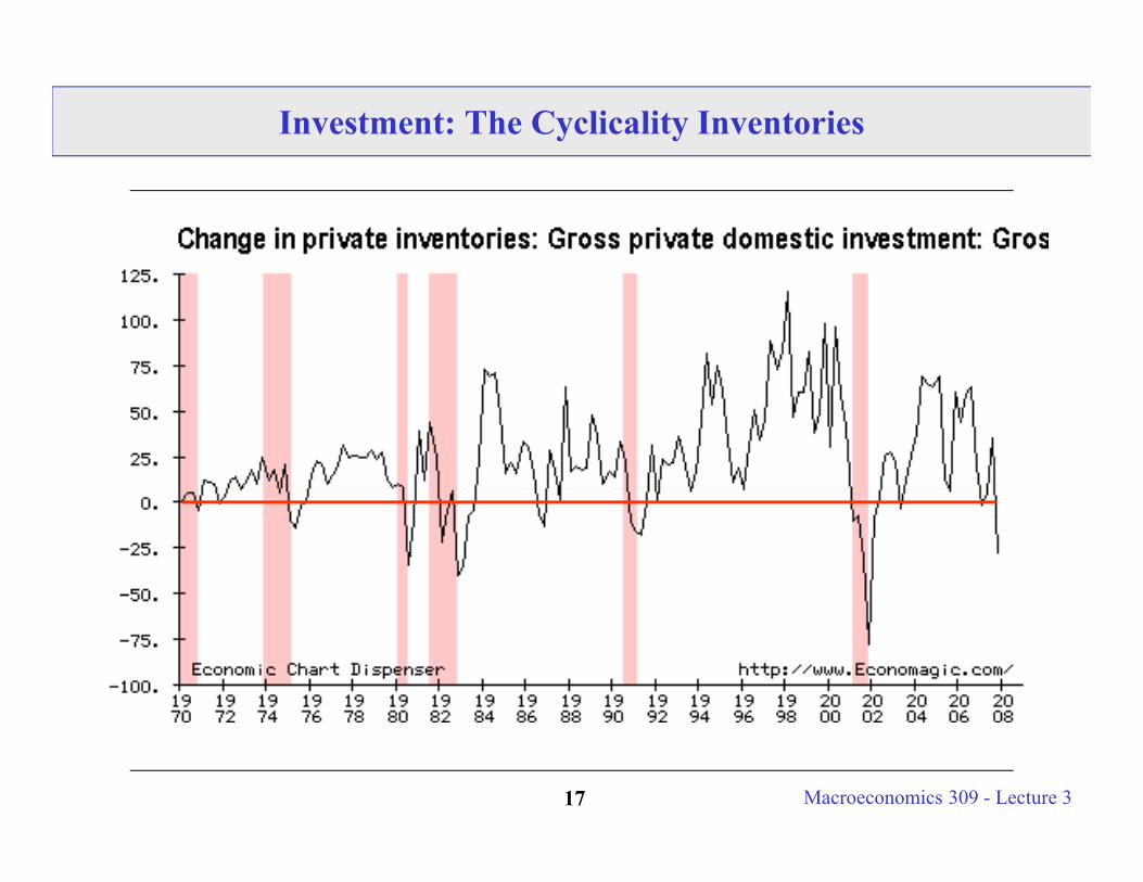
Investment is highly procyclical! (remember procyclical means – when Y increases I increases (and vice versa)).
Inventories are the most volatile (and procyclical) component of GDP.
Can inventories be a signal of future economic activity?
• Yes, can predict recessions (a rapid rise in inventories - unplanned inventories)
• Yes, can predict expansions (a smooth rise in inventories - planned inventories).
Macroeconomics 309 - Lecture 317
Investment: The Cyclicality Inventories
Macroeconomics 309 - Lecture 318
Part II: Consumption
Macroeconomics 309 - Lecture 319
An Introduction to Consumption
Major component of spending (70% of GDP).
Includes purchase of goods and services by individuals.
Two reasons why studying consumption is important:
1. It is the largest component of demand for goods and services;
2. Deciding how much to consume is linked to how much to save.
Cd = desired consumption; Sd = desired saving.
Assume income is all disposable (Yd = Y), Y - Cd - G = Sd
Macroeconomics 309 - Lecture 320
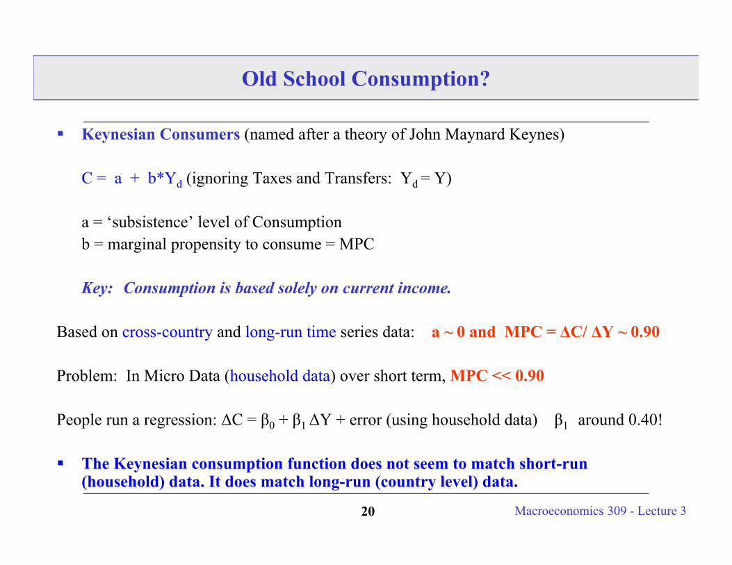
Old School Consumption?
Keynesian Consumers (named after a theory of John Maynard Keynes)
C = a + b*Yd (ignoring Taxes and Transfers: Yd = Y)
a = ‘subsistence’ level of Consumptionb = marginal propensity to consume = MPC
Key: Consumption is based solely on current income.
Based on cross-country and long-run time series data: a ~ 0 and MPC = ΔC/ ΔY ~ 0.90
Problem: In Micro Data (household data) over short term, MPC << 0.90
People run a regression: ΔC = β0 + β1 ΔY + error (using household data) β1 around 0.40!
The Keynesian consumption function does not seem to match short-run (household) data. It does match long-run (country level) data.
Macroeconomics 309 - Lecture 321
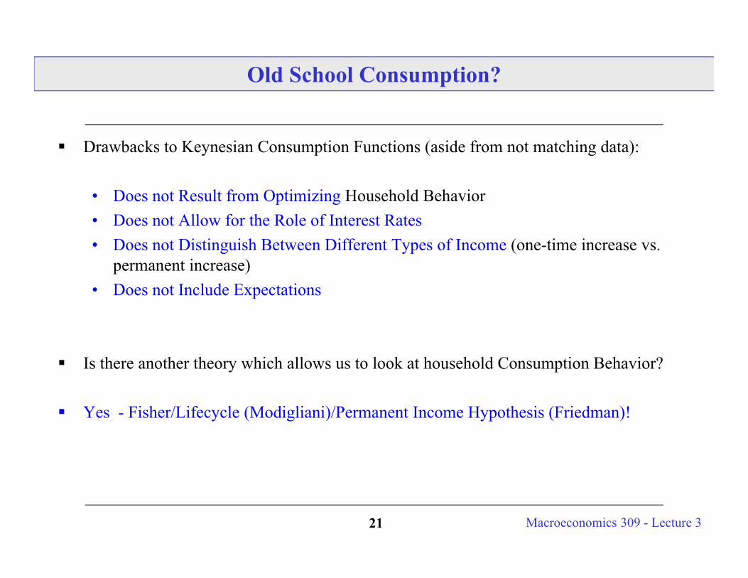
Old School Consumption?
Drawbacks to Keynesian Consumption Functions (aside from not matching data):
• Does not Result from Optimizing Household Behavior• Does not Allow for the Role of Interest Rates• Does not Distinguish Between Different Types of Income (one-time increase vs.
permanent increase) • Does not Include Expectations
Is there another theory which allows us to look at household Consumption Behavior?
Yes - Fisher/Lifecycle (Modigliani)/Permanent Income Hypothesis (Friedman)!
Macroeconomics 309 - Lecture 322
A Model of Consumption: Fisher’s Model
Fisher’s Model of Consumption allows us to look at Individual/Household Consumption Behavior.
Based on the intuition that in your consumption-saving decision you face a trade off.
Consuming more today means less saving today. Less saving today means that your resources for future consumption tomorrow are going to be lower.
Call r the real interest rate (given).
The intertemporal price of 1 extra unit of consumption today is -(1+r) less units of consumption tomorrow.
If we understand this simple point we are already half way through!
Macroeconomics 309 - Lecture 323
Set up of the Fisher’s Model of Consumption
Study the decision of an individual that lives 2 periods. (may think of them as working age and retirement).
r given.
Current and future income given, wealth given (exogenous).
Define: y = current income i.e.current wage yf = future income i.e. future wage a = initial assets i.e. wealth c = current consumption cf = future consumption
Objective: determining the choice of (c, cf)
Macroeconomics 309 - Lecture 324
Relationship between current and future resources
We call the relationship between current and future resources the (intertemporal) budget constraint.
Key: The amount of c chosen will determine the amount available for cf
y + a – c are the leftover resources that you carry to period 2 (the future).
Particularly if you put those resources in a bank you will get (y + a – c)(1 + r)
Assume that at period 2 you consume everything. It’s the last period.
We have cf = (y + a – c)(1 + r) + yf
This is the budget constraint. Let’s look at it in the (c, cf) space
Macroeconomics 309 - Lecture 325
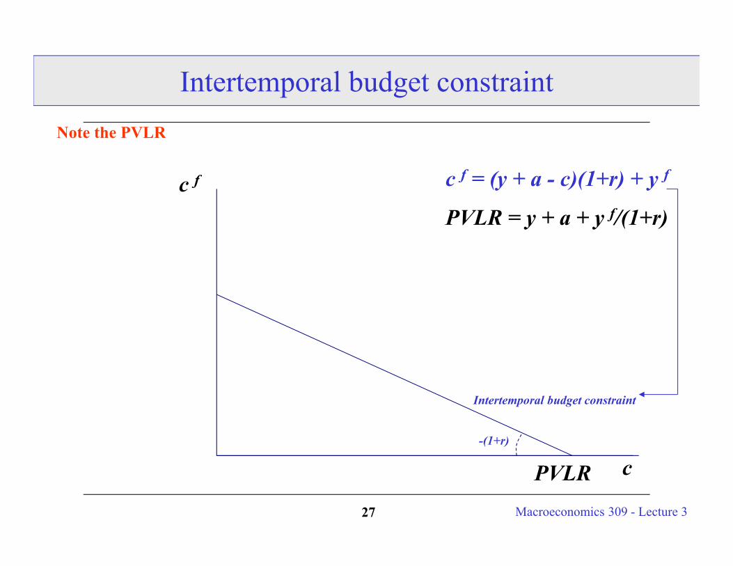
Intertemporal budget constraint
c f
-(1+r)
c
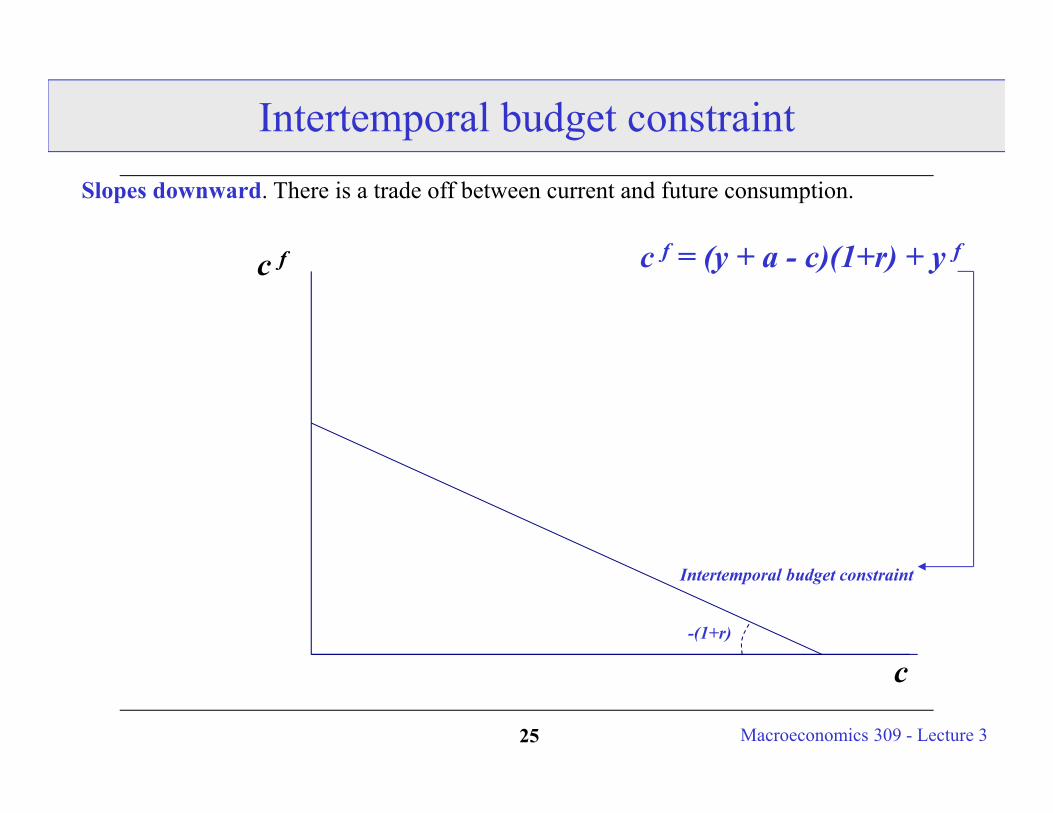
c f = (y + a - c)(1+r) + y f
Intertemporal budget constraint
Slopes downward. There is a trade off between current and future consumption.
Macroeconomics 309 - Lecture 326
Present value of lifetime resources (PVLR)
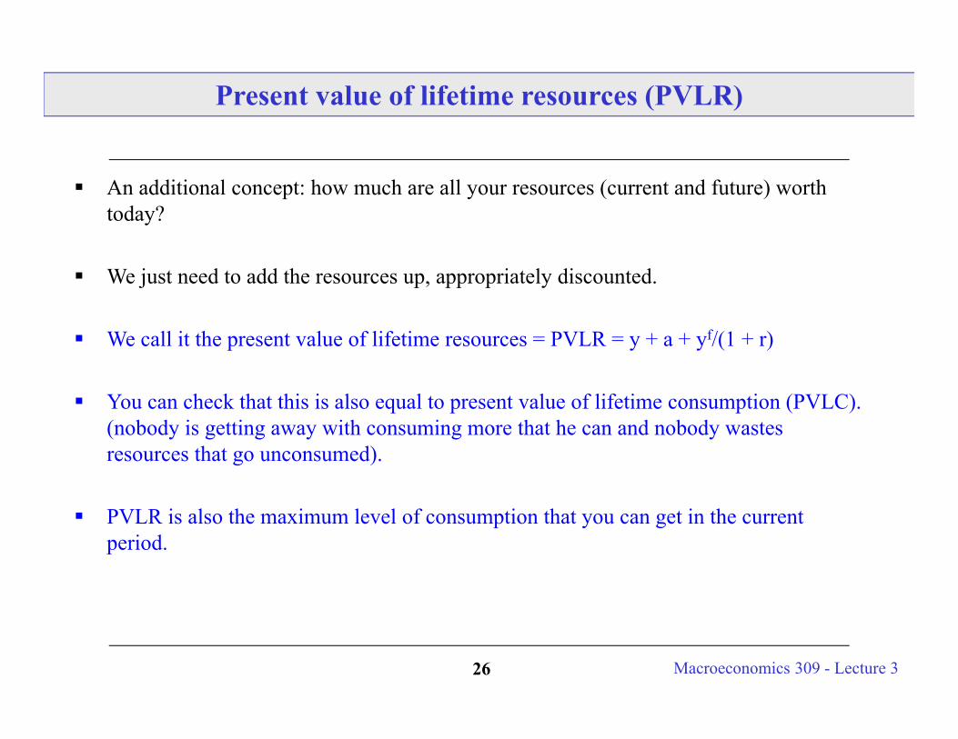
An additional concept: how much are all your resources (current and future) worth today?
We just need to add the resources up, appropriately discounted.
We call it the present value of lifetime resources = PVLR = y + a + yf/(1 + r)
You can check that this is also equal to present value of lifetime consumption (PVLC). (nobody is getting away with consuming more that he can and nobody wastes resources that go unconsumed).
PVLR is also the maximum level of consumption that you can get in the current period.
Macroeconomics 309 - Lecture 327
Intertemporal budget constraint
c f
-(1+r)
c
c f = (y + a - c)(1+r) + y f
Intertemporal budget constraint
Note the PVLR
PVLR
PVLR = y + a + y f/(1+r)
Macroeconomics 309 - Lecture 328
Last piece: Individual preferences
Our individual consumer, Giorgio, has utility U(c, cf),
Ignore their dependence on leisure for this example - makes it simpler.
(Realistically) Giorgio likes consumption (both in the present and future)
Assume c, cf are normal goods (if your income increases you want to consume more).
(Realistically) Giorgio likes if the level of consumption (c, cf) remains smooth over time (consumption smoothing, more on this later). No large drops or jumps.
So has regular indifference curves (curves representing the (c, cf) pairs that yield the same utility).

Macroeconomics 309 - Lecture 329
An Indifference Curve for Standard Preferences
c f
c
Indifference Curve (same utility on each curve)
Utility increases moving outwards
Macroeconomics 309 - Lecture 330
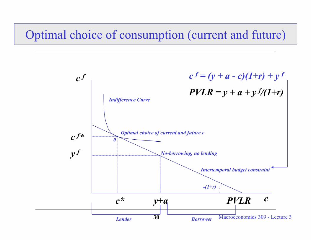
Optimal choice of consumption (current and future)
c*
c f* 0
c f
y+a
y f No-borrowing, no lending
PVLR
PVLR = y + a + y f/(1+r)
-(1+r)
c
c f = (y + a - c)(1+r) + y f
Indifference Curve
Intertemporal budget constraint
Optimal choice of current and future c
BorrowerLender
Macroeconomics 309 - Lecture 331
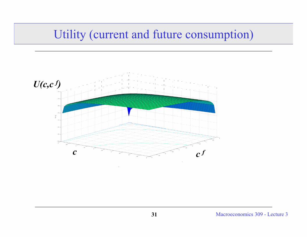
c fc
U(c,c f)
Utility (current and future consumption)
Macroeconomics 309 - Lecture 332
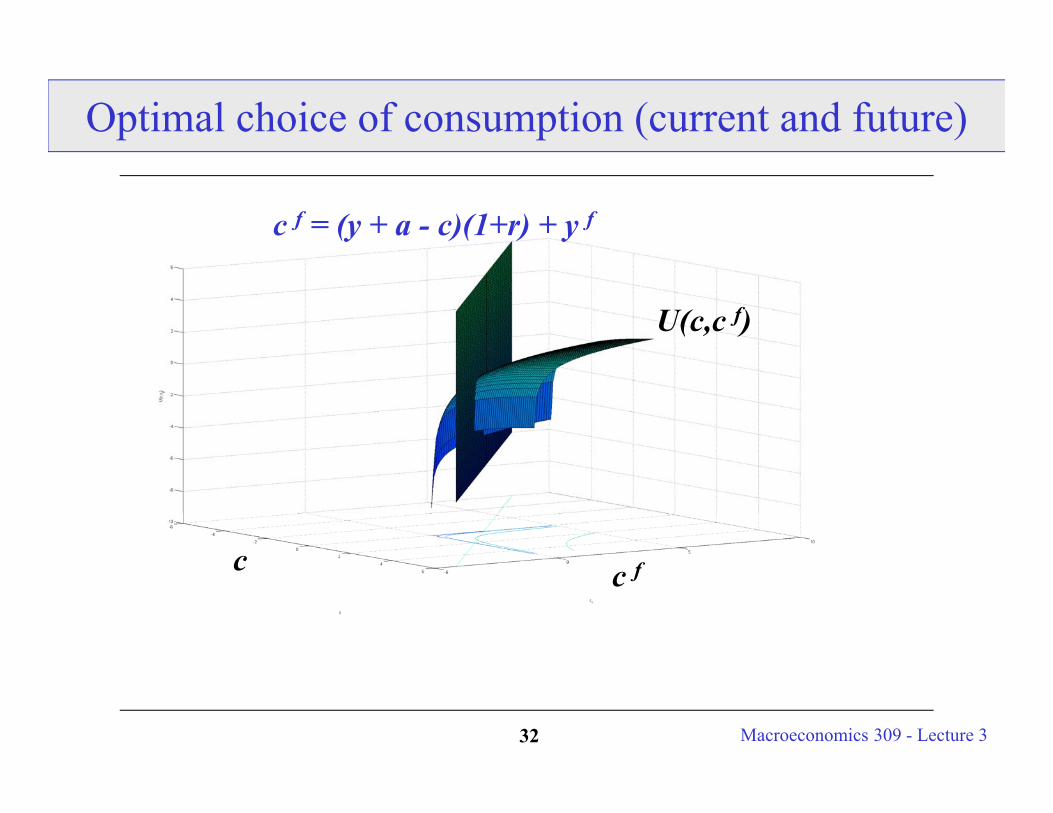
c f = (y + a - c)(1+r) + y f
c fc
U(c,c f)
Optimal choice of consumption (current and future)
Macroeconomics 309 - Lecture 333
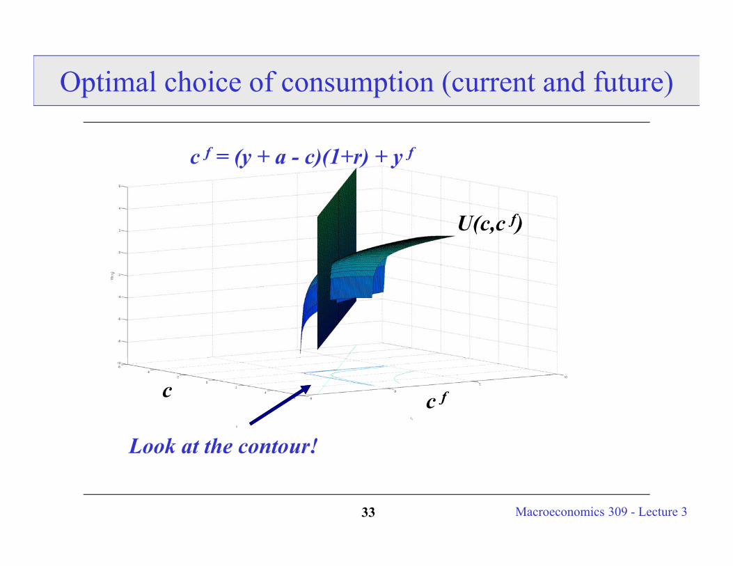
c f = (y + a - c)(1+r) + y f
c fc
U(c,c f)
Optimal choice of consumption (current and future)
Look at the contour!
Macroeconomics 309 - Lecture 334
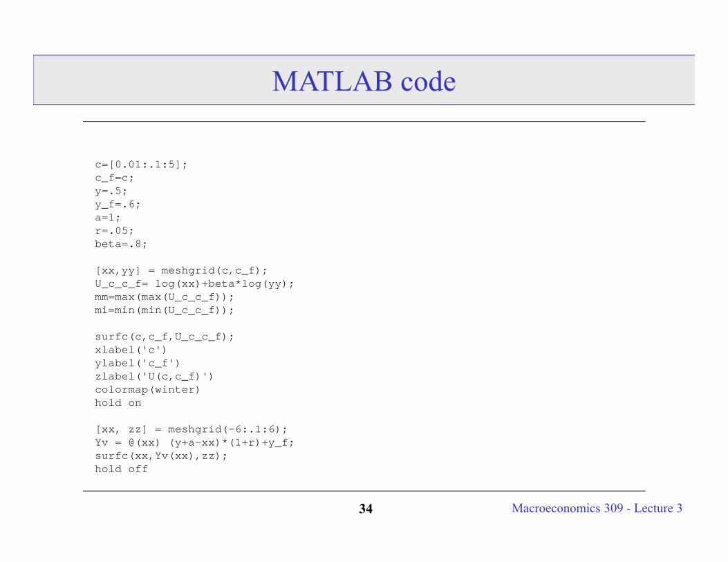
c=[0.01:.1:5];c_f=c;y=.5;y_f=.6;a=1;r=.05;beta=.8;
[xx,yy] = meshgrid(c,c_f);U_c_c_f= log(xx)+beta*log(yy);mm=max(max(U_c_c_f));mi=min(min(U_c_c_f));
surfc(c,c_f,U_c_c_f);xlabel('c')ylabel('c_f')zlabel('U(c,c_f)')colormap(winter)hold on
[xx, zz] = meshgrid(-6:.1:6);Yv = @(xx) (y+a-xx)*(1+r)+y_f;surfc(xx,Yv(xx),zz);hold off
MATLAB code
Macroeconomics 309 - Lecture 335
Fisher’s Model of Consumption
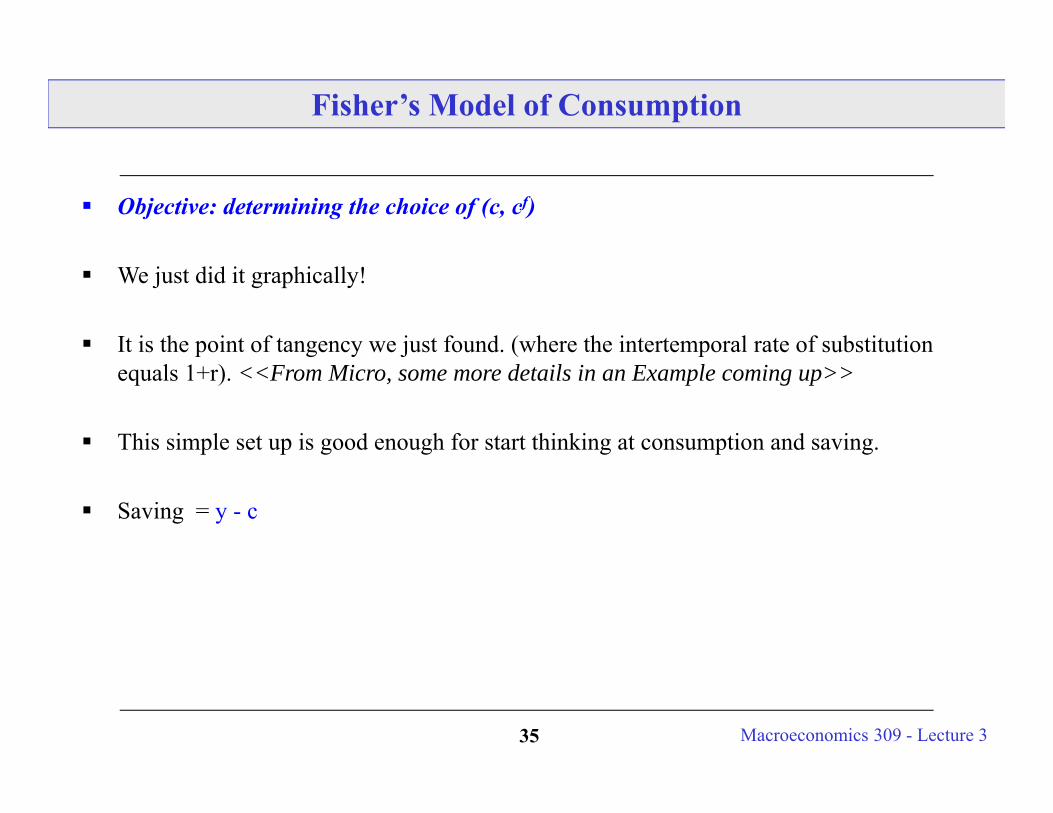
Objective: determining the choice of (c, cf)
We just did it graphically!
It is the point of tangency we just found. (where the intertemporal rate of substitution equals 1+r). <<From Micro, some more details in an Example coming up>>
This simple set up is good enough for start thinking at consumption and saving.
Saving = y - c
Macroeconomics 309 - Lecture 336
Permanent Income Hypothesis (PIH)
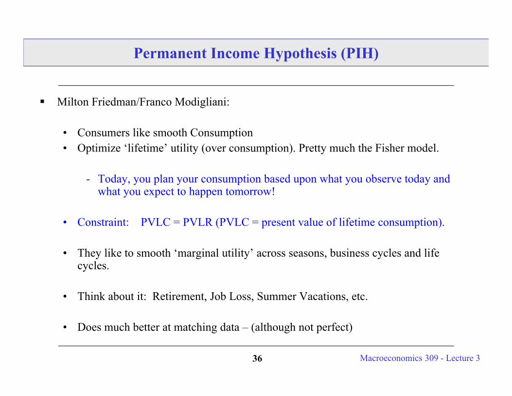
Milton Friedman/Franco Modigliani:
• Consumers like smooth Consumption• Optimize ‘lifetime’ utility (over consumption). Pretty much the Fisher model.
- Today, you plan your consumption based upon what you observe today and what you expect to happen tomorrow!
• Constraint: PVLC = PVLR (PVLC = present value of lifetime consumption).
• They like to smooth ‘marginal utility’ across seasons, business cycles and life cycles.
• Think about it: Retirement, Job Loss, Summer Vacations, etc.
• Does much better at matching data – (although not perfect)
Macroeconomics 309 - Lecture 337
From Micro: An Example of Solving the Model
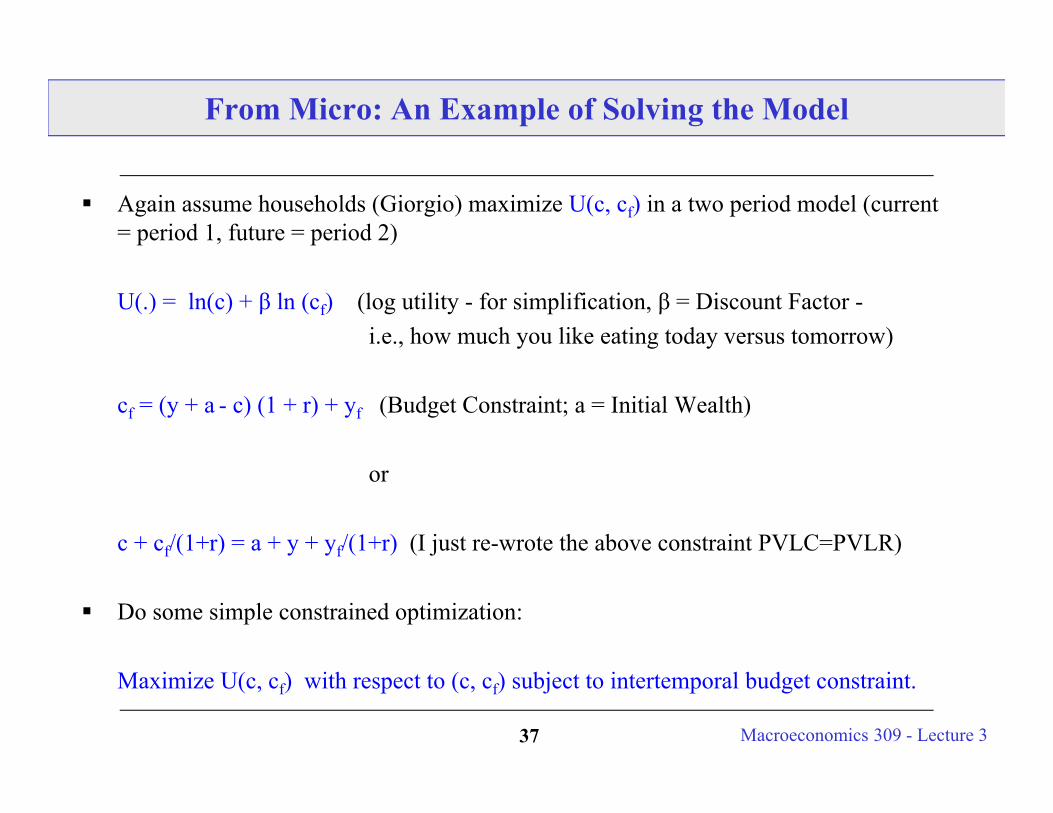
Again assume households (Giorgio) maximize U(c, cf) in a two period model (current = period 1, future = period 2)
U(.) = ln(c) + β ln (cf) (log utility - for simplification, β = Discount Factor -i.e., how much you like eating today versus tomorrow)
cf = (y + a - c) (1 + r) + yf (Budget Constraint; a = Initial Wealth)
or
c + cf/(1+r) = a + y + yf/(1+r) (I just re-wrote the above constraint PVLC=PVLR)
Do some simple constrained optimization:
Maximize U(c, cf) with respect to (c, cf) subject to intertemporal budget constraint.
Macroeconomics 309 - Lecture 338
An Example (Cont.)
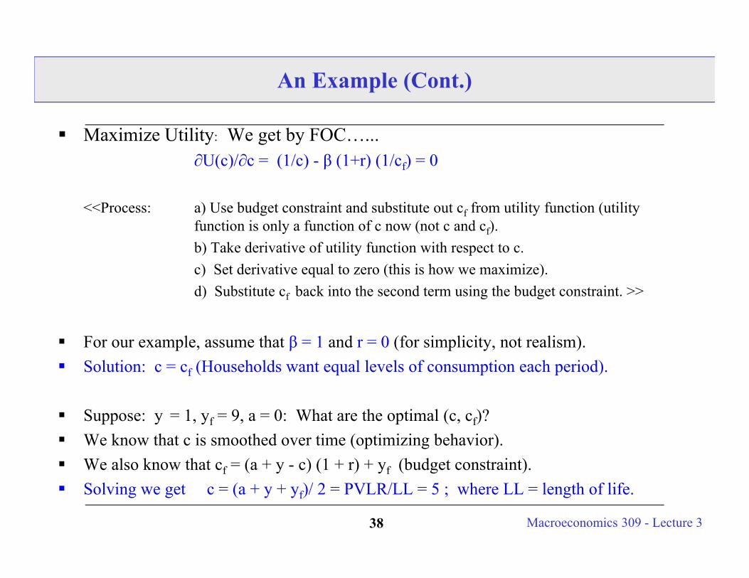
Maximize Utility: We get by FOC…...∂U(c)/∂c = (1/c) - β (1+r) (1/cf) = 0
<<Process: a) Use budget constraint and substitute out cf from utility function (utility function is only a function of c now (not c and cf).b) Take derivative of utility function with respect to c. c) Set derivative equal to zero (this is how we maximize).d) Substitute cf back into the second term using the budget constraint. >>
For our example, assume that β = 1 and r = 0 (for simplicity, not realism). Solution: c = cf (Households want equal levels of consumption each period).
Suppose: y = 1, yf = 9, a = 0: What are the optimal (c, cf)? We know that c is smoothed over time (optimizing behavior). We also know that cf = (a + y - c) (1 + r) + yf (budget constraint). Solving we get c = (a + y + yf)/ 2 = PVLR/LL = 5 ; where LL = length of life.

Macroeconomics 309 - Lecture 339
An Example (Cont.)
Period 1 2
Income 1 9Consumption 5 5Savings -4 4
Note: Expected Income Increases are already included in Today’s consumption plan:
• Only news today (about today or the future) affect our consumption plan!!• The fact that income rises from 1 to 9 between periods 1 and 2 is already included
in my consumption plan!!
Unexpected News about income, life spans, etc. WILL effect consumption decisions.
Macroeconomics 309 - Lecture 340
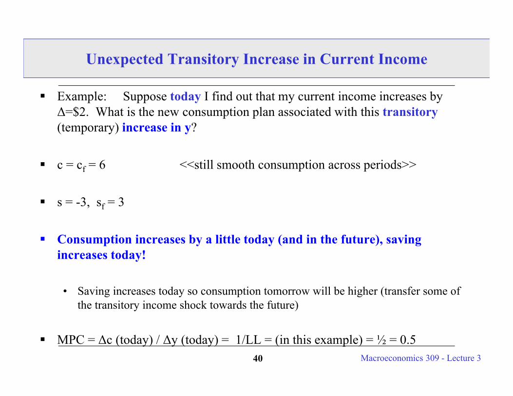
Unexpected Transitory Increase in Current Income
Example: Suppose today I find out that my current income increases by Δ=$2. What is the new consumption plan associated with this transitory(temporary) increase in y?
c = cf = 6 <<still smooth consumption across periods>>
s = -3, sf = 3
Consumption increases by a little today (and in the future), saving increases today!
• Saving increases today so consumption tomorrow will be higher (transfer some of the transitory income shock towards the future)
MPC = Δc (today) / Δy (today) = 1/LL = (in this example) = ½ = 0.5
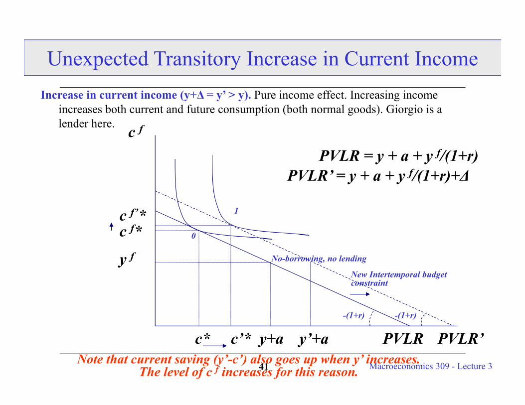
Macroeconomics 309 - Lecture 341
Unexpected Transitory Increase in Current IncomeIncrease in current income (y+Δ = y’ > y). Pure income effect. Increasing income
increases both current and future consumption (both normal goods). Giorgio is a lender here.
c*
c f* 0
c f
y+a
y f No-borrowing, no lending
PVLR
PVLR = y + a + y f/(1+r)
-(1+r) -(1+r)
PVLR’
New Intertemporal budget constraint
y’+ac’*
c f’*
Note that current saving (y’-c’) also goes up when y’ increases. The level of c f increases for this reason.
PVLR’ = y + a + y f/(1+r)+Δ
1
Macroeconomics 309 - Lecture 342
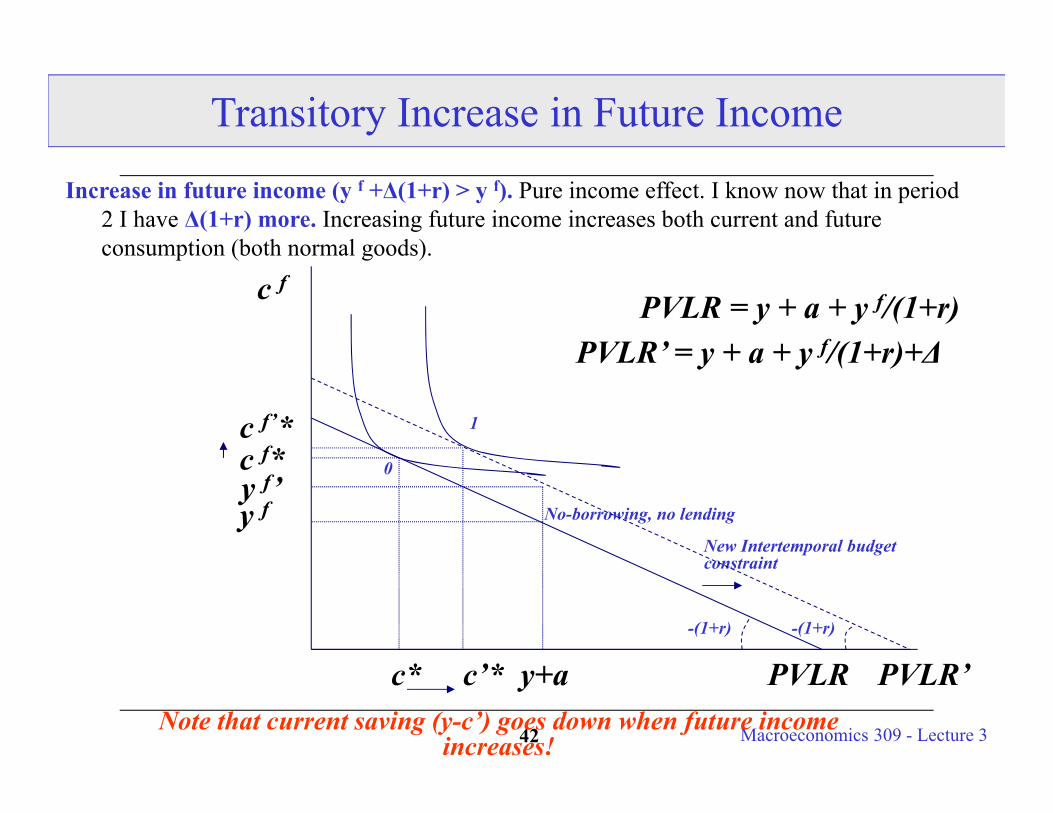
Transitory Increase in Future Income
Increase in future income (y f +Δ(1+r) > y f). Pure income effect. I know now that in period 2 I have Δ(1+r) more. Increasing future income increases both current and future consumption (both normal goods).
c*
c f* 0
c f
y+a
y f No-borrowing, no lending
PVLR
PVLR = y + a + y f/(1+r)
-(1+r) -(1+r)
PVLR’
New Intertemporal budget constraint
c’*
c f’*
Note that current saving (y-c’) goes down when future income increases!
PVLR’ = y + a + y f/(1+r)+Δ
y f’
1
Macroeconomics 309 - Lecture 343
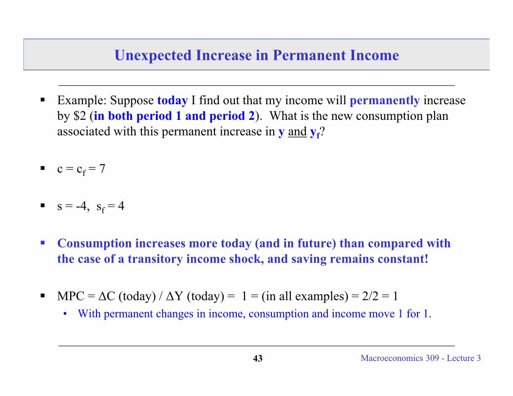
Unexpected Increase in Permanent Income
Example: Suppose today I find out that my income will permanently increase by $2 (in both period 1 and period 2). What is the new consumption plan associated with this permanent increase in y and yf?
c = cf = 7
s = -4, sf = 4
Consumption increases more today (and in future) than compared with the case of a transitory income shock, and saving remains constant!
MPC = ΔC (today) / ΔY (today) = 1 = (in all examples) = 2/2 = 1 • With permanent changes in income, consumption and income move 1 for 1.
Macroeconomics 309 - Lecture 344
Unexpected Increase in Wealth
Example: Suppose today I find out that my wealth increased by $2 prior to period 1 (a one-time unexpected stock market gain). What is the new consumption plan associated with this unexpected increase in a?
c= (a + y + yf)/ 2 = cf = 6
s = -5 (= y - c), sf = 3 (increase in PVLR due to wealth = 2)
Consumption increases today (and in future), and saving falls.
One time increases in wealth are identical to one time (transitory) changes in current income. Different effect on saving though.
Macroeconomics 309 - Lecture 345
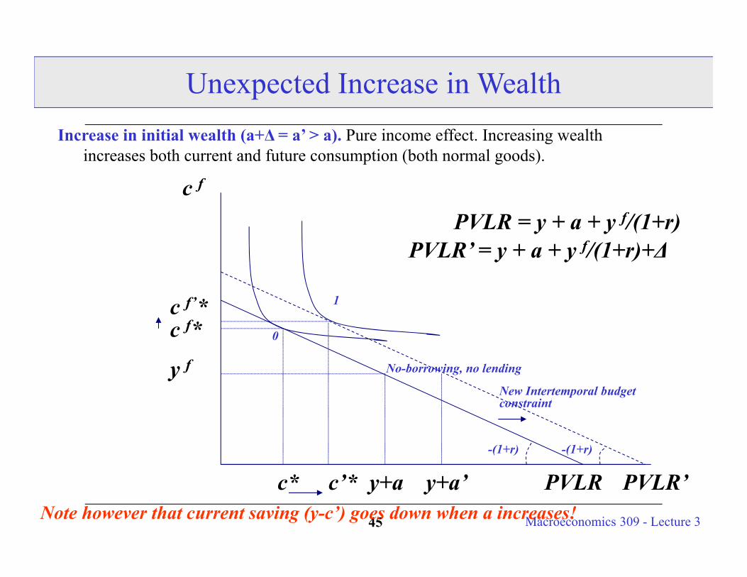
Unexpected Increase in Wealth Increase in initial wealth (a+Δ = a’ > a). Pure income effect. Increasing wealth
increases both current and future consumption (both normal goods).
c*
c f* 0
c f
y+a
y f No-borrowing, no lending
PVLR
PVLR = y + a + y f/(1+r)
-(1+r) -(1+r)
PVLR’
New Intertemporal budget constraint
y+a’c’*
c f’*
Note however that current saving (y-c’) goes down when a increases!
PVLR’ = y + a + y f/(1+r)+Δ
1
Macroeconomics 309 - Lecture 346
Some Evidence Consistent with PIH Behavior
Business Cycles are likely to be associated with temporary shocks to income.
• We find consumption to be more stable than income over the business cycle.• And the saving rate is generally procyclical.• So, C does not move 1-for-1 with Y.
Micro Studies find the MPC out of income changes to be much less than 0.9 (c does not track y one for one).
Micro Studies find a MPC out of changes in wealth of about 0.05. (Unexpected capital gains in housing/securities are like one time increases in income).
Household consumption responds more to permanent shocks to income than to temporary shocks.
Macroeconomics 309 - Lecture 347
However…
In contrast to the predictions of the PIH, consumption does vary too much with temporary income changes.
• Suppose a household earns $60,000 (on average) over 40 working years.• Total earnings over working years = $2.4 million (do not worry about discounting)• Suppose in a recession, that household loses their job for 1 year and because of transfers
(unemployment insurance, severance?) only earns $20,000 that year.• That household’s lifetime income only declined by 0.166% (less than one fifth of one
percent) …. ($40,000/$2.4 million) because of recession.• Being unemployed --- even for one full year out of a lifetime --- does not effect lifetime
income all that much!• According to the PIH, consumption should not respond that much….(household should
spread that $40,000 over 40 years. Consumption should, at most, decline only $1,000/year). • If you prepared for the possibility of job loss, consumption really shouldn’t change at all
(just draw down savings).
If this the PIH theory is true, consumption of the economy should not respond that much during recessions ((i) recessions have little effect on our lifetime incomes and (ii) we should prepare for recessions and as a result, have savings to buffer our low income).
Macroeconomics 309 - Lecture 348
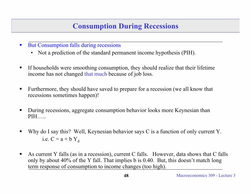
Consumption During Recessions
But Consumption falls during recessions• Not a prediction of the standard permanent income hypothesis (PIH).
If households were smoothing consumption, they should realize that their lifetime income has not changed that much because of job loss.
Furthermore, they should have saved to prepare for a recession (we all know that recessions sometimes happen)!
During recessions, aggregate consumption behavior looks more Keynesian than PIH…..
Why do I say this? Well, Keynesian behavior says C is a function of only current Y.i.e. C = a + b Yd
As current Y falls (as in a recession), current C falls. However, data shows that C falls only by about 40% of the Y fall. That implies b is 0.40. But, this doesn’t match long term response of consumption to income changes (too high).
Macroeconomics 309 - Lecture 349
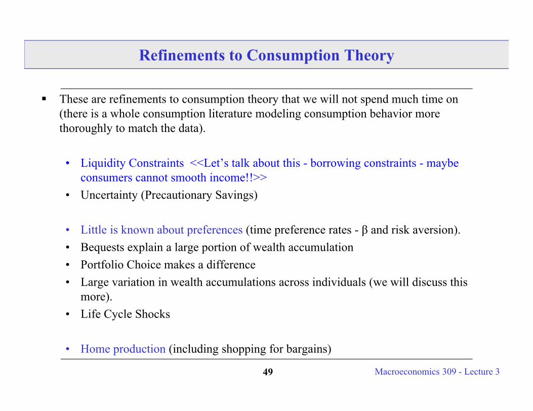
Refinements to Consumption Theory
These are refinements to consumption theory that we will not spend much time on (there is a whole consumption literature modeling consumption behavior more thoroughly to match the data).
• Liquidity Constraints <<Let’s talk about this - borrowing constraints - maybe consumers cannot smooth income!!>>
• Uncertainty (Precautionary Savings)
• Little is known about preferences (time preference rates - β and risk aversion).• Bequests explain a large portion of wealth accumulation• Portfolio Choice makes a difference• Large variation in wealth accumulations across individuals (we will discuss this
more).• Life Cycle Shocks
• Home production (including shopping for bargains)
Macroeconomics 309 - Lecture 350
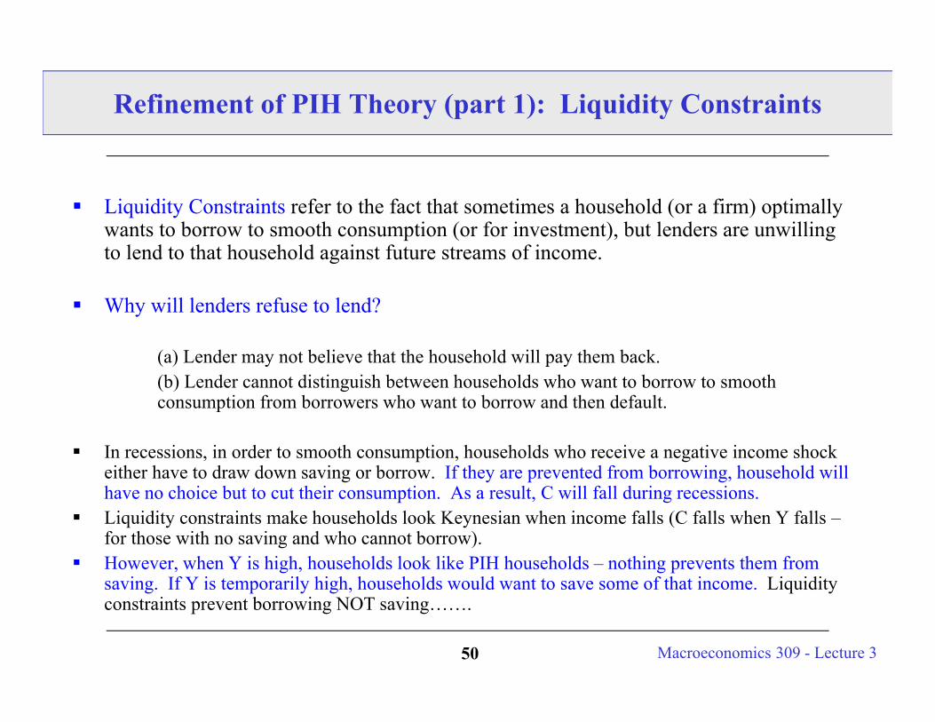
Refinement of PIH Theory (part 1): Liquidity Constraints
Liquidity Constraints refer to the fact that sometimes a household (or a firm) optimally wants to borrow to smooth consumption (or for investment), but lenders are unwilling to lend to that household against future streams of income.
Why will lenders refuse to lend?
(a) Lender may not believe that the household will pay them back.(b) Lender cannot distinguish between households who want to borrow to smooth consumption from borrowers who want to borrow and then default.
In recessions, in order to smooth consumption, households who receive a negative income shock either have to draw down saving or borrow. If they are prevented from borrowing, household will have no choice but to cut their consumption. As a result, C will fall during recessions.
Liquidity constraints make households look Keynesian when income falls (C falls when Y falls –for those with no saving and who cannot borrow).
However, when Y is high, households look like PIH households – nothing prevents them from saving. If Y is temporarily high, households would want to save some of that income. Liquidity constraints prevent borrowing NOT saving…….
Macroeconomics 309 - Lecture 351 Macroeconomics 33040 - Lecture 351
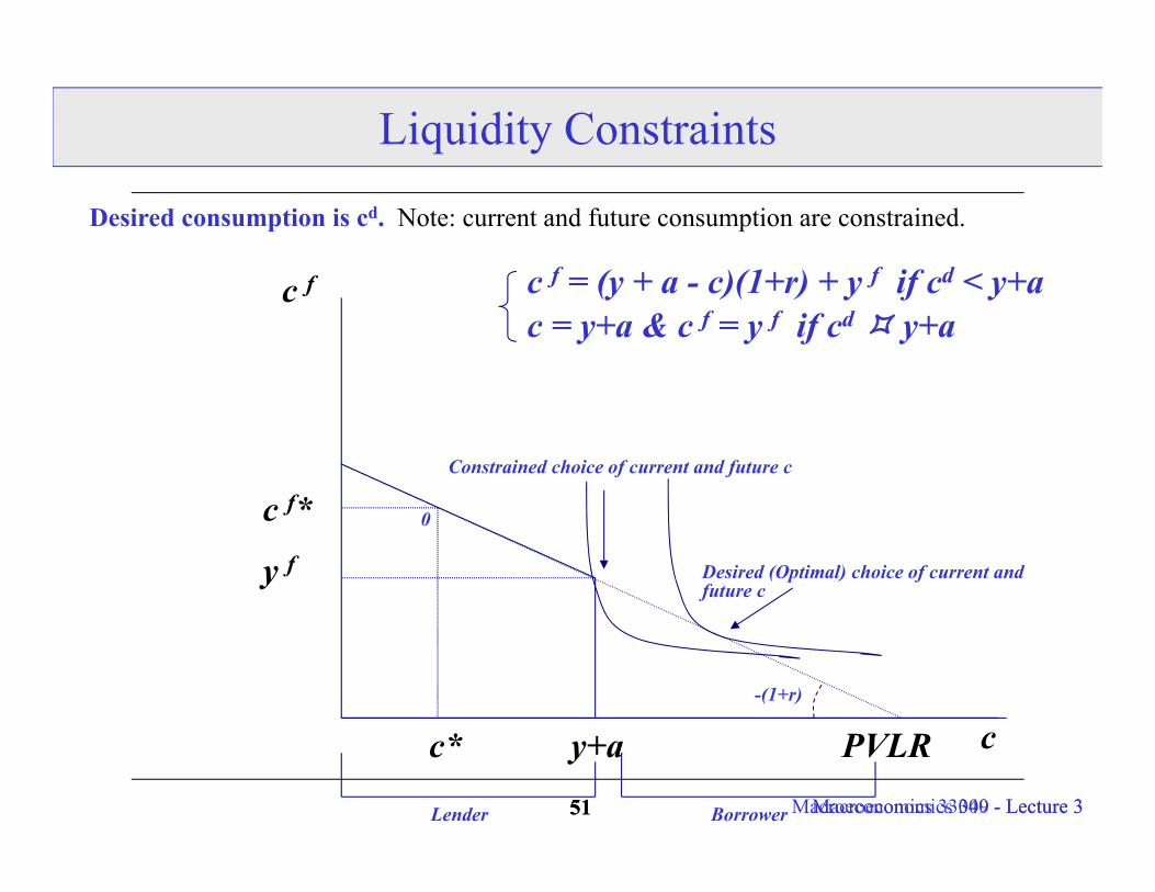
Liquidity Constraints
c*
c f* 0
c f
y+a
y f
PVLR-(1+r)
c
c f = (y + a - c)(1+r) + y f if cd < y+a
Constrained choice of current and future c
BorrowerLender
Desired (Optimal) choice of current and future c
c = y+a & c f = y f if cd y+a
Desired consumption is cd. Note: current and future consumption are constrained.
Macroeconomics 309 - Lecture 352
Refinement of PIH Theory (part 2): Grasshoppers and Ants
Perhaps the economy is made up of both Keynesian and PIH consumers:It was wintertime, the ants’ store of grain had got wet and they were laying it out to dry. A hungry grasshopper asked them to give it something to eat. ‘Why did you not gather food in the summer like us?’ the ants asked. ‘I hadn’t time’, it replied. ‘I was too busy making sweet music.’ The ants laughed at the grasshopper. ‘Very well’, they said. ‘Since you piped in the summer, now dance in the winter’. – An Aesop Fable
Fable is a a story about consumption (eating), saving (storing food) and retirement (winter)…..
Suppose the population is made up of both economic grasshoppers (Keynesian consumers) and ants (PIH consumers).
The ants in the parable were forward looking (like PIH theory suggests – they know retirement is coming and prepare for it).
The grasshoppers eat their current income and do little saving. They behave as if retirement does not exist. When retirement comes, they do not have enough recourses to sustain their consumption. <<we can also think of winter as a recession…the grasshoppers do not prepare for recessions>>
As a result, the consumption of grasshoppers will respond to predictable changes in income (recessions, retirement, etc.)
Macroeconomics 309 - Lecture 353
Grasshoppers and Ants: Evidence
About 20% of households behave according to Keynesian theories (increasing consumption with income without regard for future states of the world).
A full 1/3 of the baby boom generation is ‘ill prepared’ to sustain consumption through retirement (Bill Gale, Brookings).
Over 20% of households do not own a checking/saving account (over 50% of African American Households) - (40% have less than $5k in liquid assets).
Observe ‘Grasshopper’ behavior among households in the population (consumption responds to both predictable income increases and predictable income declines). These same households are ill prepared for retirement.
Pseudo-Keynesian behavior important for policy!• Keynesian’s will have large current response to temporary tax cuts.• PIH households (who are not liquidity constrained) will have very small response
to temporary tax cuts.
Macroeconomics 309 - Lecture 354 Macroeconomics 33040 - Lecture 354
Refinement of PIH Theory (part 3): Home Production
We measure consumption (as with most macro variables) in dollars. Expenditure may not be a good measure of consumption when the value of time changes.
When the value of time is low (unemployment – like in recessions) or retirement, individuals can take action to reduce their expenditure (holding consumption constant).
• Clip coupons• Search for bargains across stores• Make your lunch at home instead of buying it at a cafeteria.
If home production/search is important, we would expect EXPENDITURE to fall during a recession. However, CONSUMPTION may remain unchanged!
Strong evidence for the home production/search theory of consumption expenditures. The decline in expenditure during recessions does not mean people are consuming less.
Macroeconomics 309 - Lecture 355
Consumption and Interest Rates
So far we have focused at changes in income and wealth.
Now let’s analyze what are the consequences of changes in prices.
1+the real interest rate is the price of today’s consumption relative to future consumption. You forgo 1+r dollars of future consumption to consume 1 dollar today.
An increase in the real interest rate produces an increase of the price of today’s consumption relative to future consumption.
Macroeconomics 309 - Lecture 356
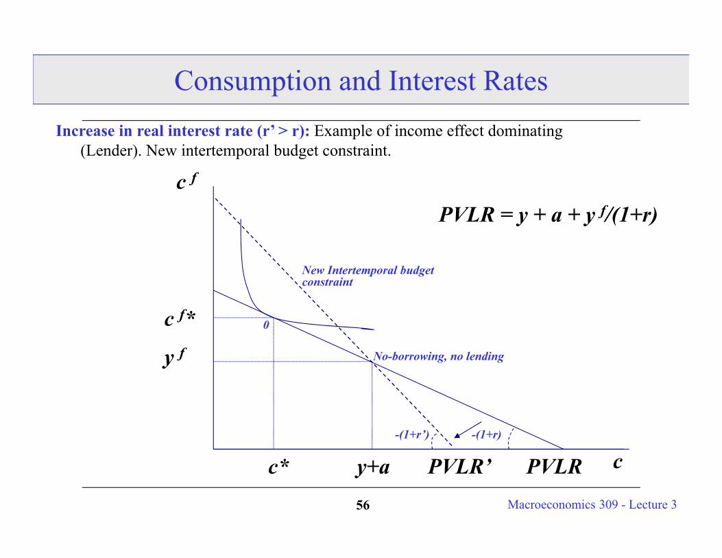
Consumption and Interest RatesIncrease in real interest rate (r’ > r): Example of income effect dominating
(Lender). New intertemporal budget constraint.
c*
c f* 0
c f
y+a
y f No-borrowing, no lending
PVLR
PVLR = y + a + y f/(1+r)
-(1+r)-(1+r’)
cPVLR’
New Intertemporal budget constraint
Macroeconomics 309 - Lecture 357
Substitution and Income Effects: Intuition
Assume current and future consumption are normal goods.
1+the real interest rate is the price of today’s consumption relative to future consumption: You forgo 1+r dollars of future consumption to consume 1 dollar today.
Increase in the real interest rate => Increase of the price of today’s consumption relative to future consumption.
The fact that you shift away from current consumption (i.e. you increase your saving) as a consequence of this change in price is the substitution effect. Cheaper future consumption produces an incentive to consume less today and save more.
But an increase in r also affects income (hence an income effect):1. An increase in the real interest rate increases interest receipts for a lender. This
produces an incentive to consume more today and save less.2. An increase in the real interest rate increases interest payments for a borrower.
This produces an incentive to consume less today and save more.
Macroeconomics 33040 - Lecture 358
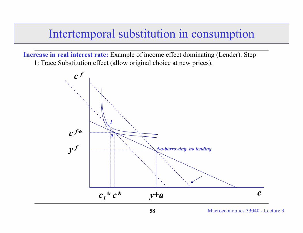
Intertemporal substitution in consumption Increase in real interest rate: Example of income effect dominating (Lender). Step
1: Trace Substitution effect (allow original choice at new prices).
c*
c f*1
0
c1*
c f
y+a
y f No-borrowing, no lending
c
Macroeconomics 33040 - Lecture 359
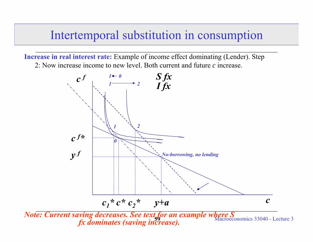
Intertemporal substitution in consumption Increase in real interest rate: Example of income effect dominating (Lender). Step
2: Now increase income to new level. Both current and future c increase.
cc*
c f*
S fxI fx
1
0
2
011 2
c2*c1*
c f
y+a
y f No-borrowing, no lending
Note: Current saving decreases. See text for an example where S fx dominates (saving increase).
Macroeconomics 33040 - Lecture 360
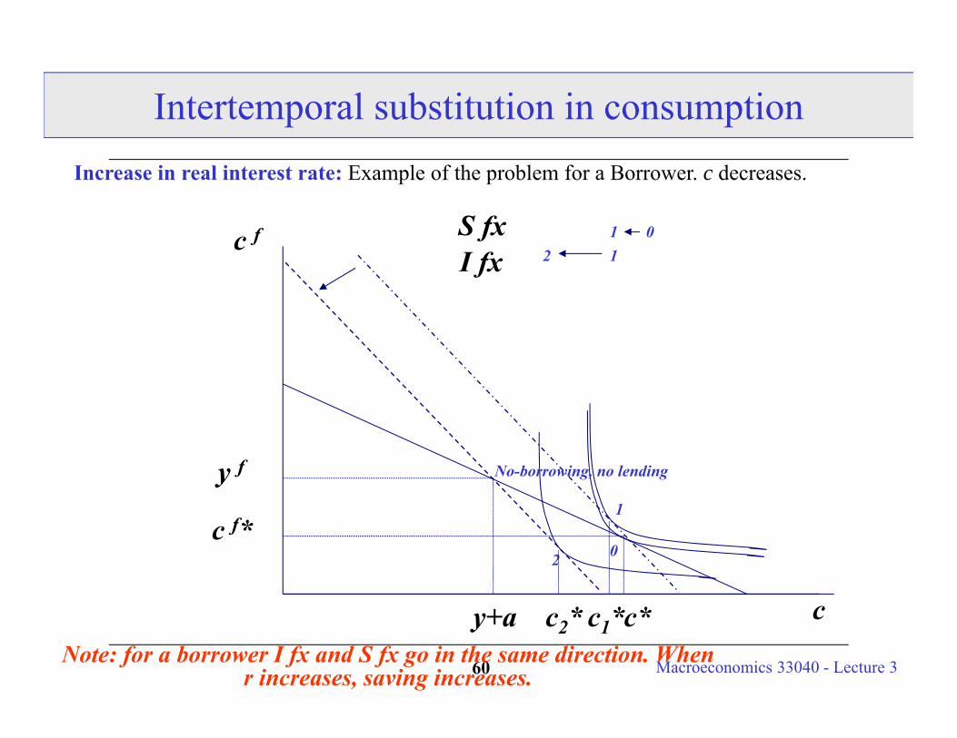
Intertemporal substitution in consumption Increase in real interest rate: Example of the problem for a Borrower. c decreases.
cc*
c f*
S fxI fx
1
02
0112
c2* c1*
c f
y+a
y f No-borrowing, no lending
Note: for a borrower I fx and S fx go in the same direction. When r increases, saving increases.
Macroeconomics 309 - Lecture 361
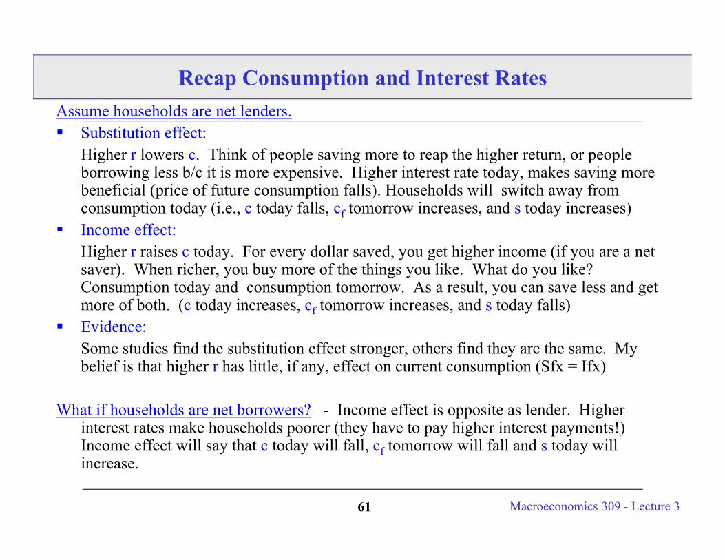
Recap Consumption and Interest RatesAssume households are net lenders. Substitution effect:
Higher r lowers c. Think of people saving more to reap the higher return, or people borrowing less b/c it is more expensive. Higher interest rate today, makes saving more beneficial (price of future consumption falls). Households will switch away from consumption today (i.e., c today falls, cf tomorrow increases, and s today increases)
Income effect:Higher r raises c today. For every dollar saved, you get higher income (if you are a net saver). When richer, you buy more of the things you like. What do you like? Consumption today and consumption tomorrow. As a result, you can save less and get more of both. (c today increases, cf tomorrow increases, and s today falls)
Evidence:Some studies find the substitution effect stronger, others find they are the same. My belief is that higher r has little, if any, effect on current consumption (Sfx = Ifx)
What if households are net borrowers? - Income effect is opposite as lender. Higher interest rates make households poorer (they have to pay higher interest payments!) Income effect will say that c today will fall, cf tomorrow will fall and s today will increase.
Macroeconomics 309 - Lecture 362
Full Recap of the Fisher/PIH model
Assume current and future consumption are normal goods.
An increase in current income increases current and future consumption and increases saving.
An increase in future income or wealth increases current and future consumption but decreases saving.
An increase in the real interest rate decreases current consumption but increases future consumption and saving for a lender, if the substitution effect dominates.
An increase in the real interest rate increases current and future consumption but decreases saving for a lender, if the income effect dominates.
An increase in the real interest rate decreases current consumption and increases saving for a borrower. May increase or decrease future consumption.
Macroeconomics 33040 - Lecture 363
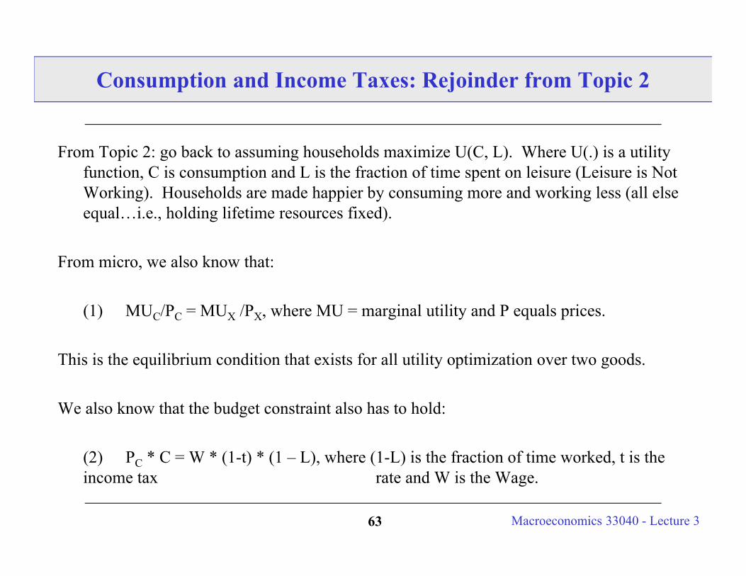
Consumption and Income Taxes: Rejoinder from Topic 2
From Topic 2: go back to assuming households maximize U(C, L). Where U(.) is a utility function, C is consumption and L is the fraction of time spent on leisure (Leisure is Not Working). Households are made happier by consuming more and working less (all else equal…i.e., holding lifetime resources fixed).
From micro, we also know that:
(1) MUC/PC = MUX /PX, where MU = marginal utility and P equals prices.
This is the equilibrium condition that exists for all utility optimization over two goods.
We also know that the budget constraint also has to hold:
(2) PC * C = W * (1-t) * (1 – L), where (1-L) is the fraction of time worked, t is the income tax rate and W is the Wage.
Macroeconomics 33040 - Lecture 364
Consumption and Income Taxes (continued)
Suppose income taxes fall….. What has to happen to consumption and leisure???? Income Effect (Equation 2 on previous slide)When income taxes fall – equation 2 says that, all else equal, households will be richer [i.e.,
(W(1-t)) will increase].When households are richer, they will buy more of the things they like.What do households like?........ C and L.
So, according to income effect, C and L will increase when income taxes fall.Substitution Effect (Equation 1 on previous slide)When income taxes fall, equation 1 says that, all else equal, after tax wages will increase
[i.e., (W(1-t) will increase].As the price of leisure increases, MUx must increase AND/OR MUC must fall. As X falls, MUX increases (law of diminishing marginal utility of X).As C increases, MUX must fall
So, according to substitution effect, C will increase and L will fall when income taxes fall.
Putting two effects together: Effect on L is ambiguous. C will definitely increase!
Macroeconomics 309 - Lecture 365
Summary: What effects consumption
Current Income (Both PIH and Keynesian Theories) Expectations of Future Income (Only PIH theory)
Wealth Temporary vs. Permanent Changes Tax Policy Interest rates (slightly)
Preferences
The magnitude of the results depend on whether consumers follow Keynesian or PIH consumption rules and whether or not liquidity constraints exist!!!!
In our Government Policy Lecture, we will talk about Social Security Systems and Consumer’s Expectations of Tax Changes
Macroeconomics 309 - Lecture 366
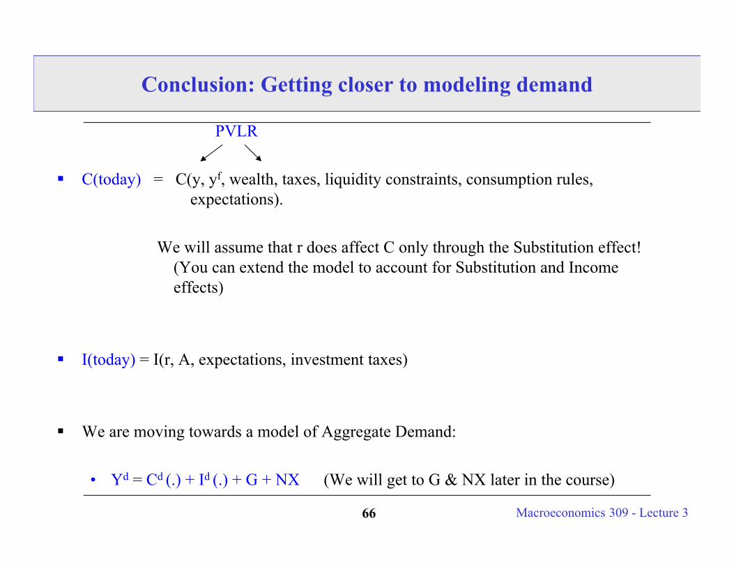
Conclusion: Getting closer to modeling demand
PVLR
C(today) = C(y, yf, wealth, taxes, liquidity constraints, consumption rules, expectations).
We will assume that r does affect C only through the Substitution effect! (You can extend the model to account for Substitution and Income effects)
I(today) = I(r, A, expectations, investment taxes)
We are moving towards a model of Aggregate Demand:
• Yd = Cd (.) + Id (.) + G + NX (We will get to G & NX later in the course)