Embed Size (px)
Citation preview

NBER WORKING PAPER SERIES
PRECAUTIONARY SAVING AND CONSUMPTION SMOOTHING ACROSS TIMEAND POSSIBILITIES
Miles KimballPhilippe Weil
Working Paper 3976http://www.nber.org/papers/w3976
NATIONAL BUREAU OF ECONOMIC RESEARCH1050 Massachusetts Avenue
Cambridge, MA 02138January 1992
We gratefully acknowledge support from the National Science Foundation. Part of this research wasfunded by National Institute of Aging Grants P01-AG10179 and 5 P01 AG026571-03. Our researchassistant, Thomas Bishop, caught many small errors and made excellent suggestions for tighteningup the text. We thank an anonymous referee for useful comments and suggestions. The views expressedherein are those of the author(s) and do not necessarily reflect the views of the National Bureau ofEconomic Research.
© 1992 by Miles Kimball and Philippe Weil. All rights reserved. Short sections of text, not to exceedtwo paragraphs, may be quoted without explicit permission provided that full credit, including © notice,is given to the source.
Precautionary Saving and Consumption Smoothing Across Time and PossibilitiesMiles Kimball and Philippe WeilNBER Working Paper No. 3976January 1992, Revised July 2008JEL No. E21,D11
ABSTRACT
This paper examines how aversion to risk and aversion to intertemporal substitution determine thestrength of the precautionary saving motive in a two-period model with Selden/Kreps-Porteus preferences.For small risks, we derive a measure of the strength of the precautionary saving motive which generalizesthe concept of "prudence" introduced by Kimball (1990b). For large risks, we show that decreasingabsolute risk aversion guarantees that the precautionary saving motive is stronger than risk aversion,regardless of the elasticity of intertemporal substitution. Holding risk preferences fixed, the extentto which the precautionary saving motive is stronger than risk aversion increases with the elasticityof intertemporal substitution. We derive sufficient conditions for a change in risk preferences aloneto increase the strength of the precautionary saving motive and for the strength of the precautionarysaving motive to decline with wealth. Within the class of constant elasticity of intertemporal substitution,constant-relative risk aversion utility functions, these conditions are also necessary.
Miles KimballDepartment of EconomicsUniversity of MichiganAnn Arbor, MI 48109-1220and [email protected]
Philippe WeilDirector, Universite Libre de BruxellesECARES50, Avenue Roosevelt CP 114B-1050 Brussels BELGIUMand [email protected]

1 Introduction
Because it does not distinguish between aversion to risk and aversion to intertemporal sub-
stitution, the traditional theory of precautionary saving based on intertemporal expected
utility maximization is a framework within which one cannot ask questions that are funda-
mental to the understanding of consumption in the face of labor income risk. For instance,
how does the strength of the precautionary saving motive vary as the elasticity of intertem-
poral substitution changes, holding risk aversion constant? Or, how does the strength of
the precautionary saving motive vary as risk aversion changes, holding the elasticity of
intertemporal substitution constant?
Moreover, one might wonder whether some of the results from an intertemporal ex-
pected utility framework continue to hold once one distinguishes between aversion to risk
and resistance to intertemporal substitution. For instance, does decreasing absolute risk
aversion imply that the precautionary saving motive is stronger than risk aversion regard-
less of the elasticity of intertemporal substitution? And under what conditions does the
precautionary saving motive decline with wealth?
To make sense of these questions, and to gain a better grasp on the channels through
which precautionary saving may affect the economy,1 we adopt a representation of pref-
erences based on the Selden and Kreps-Porteus axiomatization, which separates attitudes
towards risk and attitudes towards intertemporal substitution.2
The existing literature on the theory of precautionary saving under Selden/Kreps-
Porteus preferences is not very extensive. Barsky (1986) addresses some of the aspects
of this theory in relation to rate-of-return risks in a two-period setup, Weil (1993) analyzes
a parametric infinite-horizon model with mixed isoelastic/constant absolute risk aversion
1 There has been a considerable resurgence of interest in precautionary saving in the last twenty-two years.For some early papers in this period, see for instance Barsky, Mankiw, and Zeldes (1986), Skinner (1988),Kimball and Mankiw (1989), Zeldes (1989), Caballero (1990), Kimball (1990b), and Weil (1993). The subse-quent citation patterns of these early papers indicate continuing interest in precautionary saving.
2See, for instance, Selden (1978), Selden (1979), Kreps and Porteus (1978), Hall (1988), Epstein and Zin(1989), Farmer (1990), Weil (1990), and Hansen, Sargent, and Tallarini (1999).

preferences (which do not allow one to look at the consequences of decreasing absolute risk
aversion), but there has not been as yet any systematic treatment of precautionary saving
under Selden/Kreps-Porteus preferences.
Under intertemporal expected utility maximization, the strength of the precautionary
saving motive is not an independent quantity, but is linked to other aspects of risk pref-
erences. In that case, the absolute prudence −v′′′/v′′ of a von-Neumann Morgenstern
second-period utility function v measures the strength of the precautionary saving motive
(see Kimball (1990b)]), and there is an identity linking prudence to risk aversion under
additively time- and state-separable utility:
−v′′′(x)
v′′(x)= a(x)−
a′(x)
a(x), (1.1)
where
a(x) = −v′′(x)
v′(x)(1.2)
is the Arrow-Pratt measure of absolute risk aversion. Similarly, the coefficient of relative
prudence −x v′′′(x)/v′′(x) satisfies
−x v′′′(x)
v′′(x)= γ(x) + ǫ(x), (1.3)
where
γ(x) =−x v′′(x)
v′(x)= xa(x) (1.4)
is relative risk aversion, and
ǫ(x) =−xa′(x)
a(x)(1.5)
is the elasticity of absolute risk tolerance,3 which approximates the wealth elasticity of risky
investment.
The purpose of this paper is to determine what links exist—in the more general
3Absolute risk tolerance is defined as the reciprocal of absolute risk aversion: 1/a(x).
2
Selden/Kreps-Porteus framework that allows for risk preferences and intertemporal sub-
stitution to be varied independently from each other—between the strength of the precau-
tionary saving motive, risk aversion, and intertemporal substitution.
In Section 2, we set up the model. In Section 3 we derive a local measure of the
precautionary saving motive for small risks. Section 4 deals with large risks: it performs
various comparative statics experiments to provide answers to the questions we asked in
our first two paragraphs. The conclusion discusses the implications of our main results.
2 Setup
This section describes our basic model, and characterizes optimal consumption and saving
decisions.
2.1 The model
We use essentially the same two-period model of the consumption-saving decision as in
Kimball (1990b), except for departing from the assumption of intertemporal expected util-
ity maximization.4 We assume that the agent can freely borrow and lend at a fixed risk-free
rate, and that the constraint that an agent cannot borrow against more than the minimum
value of human wealth is not binding at the end of the first period. Since the interest rate
is exogenously given, all magnitudes can be represented in present-value terms— so that,
without loss of generality, the real risk-free rate can be assumed to be zero. We also assume
that labor supply is inelastic, so that labor income can be treated like manna from heaven.
Finally, we assume that preferences are additively time-separable.
4Because there is enough to be said about the two-period case, we leave comprehensive treatment of themulti-period case to future research. ? follows up our research by studying the multi-period case computa-tionally. The results derived by Weil (1993) and van der Ploeg (1993) for particular multi-period parametricversions of Kreps-Porteus preferences suggest that the two-period results of this paper have natural general-izations to multi-period settings. In the case of intertemporal expected utility maximization, Kimball (1990a)extends two-period results about precautionary saving effects decreasing with wealth to multi-period settings.As in that paper, characterization of the multiperiod case must rely on the tools developed in the two-periodcase. In addition, the two-period model highlights what cannot possibly be proven for the multiperiod case.
3

The preferences of our agent can be represented in two equivalent ways. First, there is
the Selden ordinal certainty equivalence representation,
u(c1) + U(v−1(E v(c2))) = u(c1) + U(M(c2)),
where c1 and c2 are first- and second-period consumption, u is the first-period utility func-
tion, U is the second-period utility function for the certainty equivalent of random second-
period consumption (computed according to the atemporal von Neumann-Morgenstern
utility function v),5 E is an expectation conditional on all information available during
the first period, and M is the certainty equivalent operator associated with v:
M(c2) = v−1(E v(c2)).
According to this representation, the utility our consumer derives from the consumption
lottery (c1, c2) is the sum of the felicity provided by c1 and the felicity provided by the
certainty equivalent M(c2) of c2. Obviously, v plays no role, and M is an identity, under
certainty. These functions thus capture pure risk preferences.
Second, there is the Kreps-Porteus representation,
u(c1) +φ(E v(c2)),
where nonlinearity of the function φ indicates departure from intertemporal expected util-
ity maximization. This formulation expresses total utility as the nonlinear aggregate of
current felicity and expected future felicity.6
These two representations are equivalent as long as v is a continuous, monotonically
increasing function, so that M(c2) is well defined whenever E v(c2) is well defined. The
5Since U is a general function, any time discounting can be embedded in the functional form of U .6Thus, when we refer in this paper to the Kreps-Porteus representation or to Kreps-Porteus preferences,
we point to the specific form of the aggregator function between current and future consumption proposed byKreps and Porteus (1978) in their multi-period axiomatization.
4

link between the two representations is that
φ(ν) = U(v−1(ν)). (2.1)
Thus, as can be seen by straightforward differentiation, φ is concave if −U ′′/U ′ ≥ −v′′/v′,
while φ is convex if −U ′′/U ′ ≤ −v′′/v′. We will mainly use the Selden representation—
which is more intuitive—but, when more convenient mathematically, we use the Kreps-
Porteus representation.
2.2 Optimal consumption and saving
Our consumer solves the following problem:
maxx
u(w − x) + U(M(x + y)), (2.2)
where w is the sum of initial wealth, first-period income, and the mean of second-period
income, x is “saving” out of this whole sum, and y is the deviation of second-period income
from its mean.
The first-order condition for the optimal level of saving x is
u′(w − x) = U ′(M(x + y))M ′(x + y), (2.3)
where M ′ is defined by
M ′(x + y) =∂
∂ xM(x + y). (2.4)
To guarantee that the solution to (2.3) is uniquely determined, we would like the
marginal utility of saving,
U ′(M(x + y))M ′(x + y),
to be a decreasing function of x .7 In the main body of the paper, we will simply assume7Throughout the paper, verbal characterizations of gradients (increasing, decreasing) or inequalities
5
that this condition holds; it is equivalent to the reasonable assumption that first-period
consumption is a normal good. Appendix A gives a deeper treatment, proving that the
marginal utility of saving is decreasing under plausible restrictions on preferences.
Equation (2.3) and the assumption of a decreasing marginal utility of saving imply that
the uncertainty represented by y will cause additional saving if
U ′(M(x + y))M ′(x + y)> U ′(x), (2.5)
that is, if the risk y raises the marginal utility of saving.
As in Kimball (1990b), we can study the strength of precautionary saving effects by
looking at the size of the precautionary premium θ ∗ needed to compensate for the effect of
the risk y on the marginal utility of saving. The precautionary premium θ ∗ is the solution
to the equation
U ′(M(x + θ ∗+ y))M ′(x + θ ∗ + y) = U ′(x), (2.6)
or equivalently, using the Kreps-Porteus representation of preferences, the solution to the
equation
φ′[E v(x + θ ∗+ y)]E v′(x + θ ∗ + y) = φ′[v(x)]v′(x). (2.7)
To be more specific, θ ∗ is the compensating Kreps-Porteus precautionary premium. It gen-
eralizes the compensating von Neumann-Morgenstern precautionary premium ψ∗ that is
defined8 as the solution to
E v′(x +ψ∗+ y) = v′(x). (2.8)
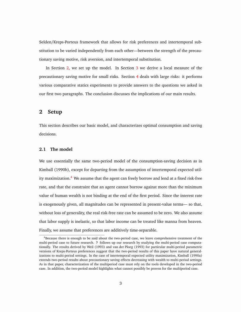
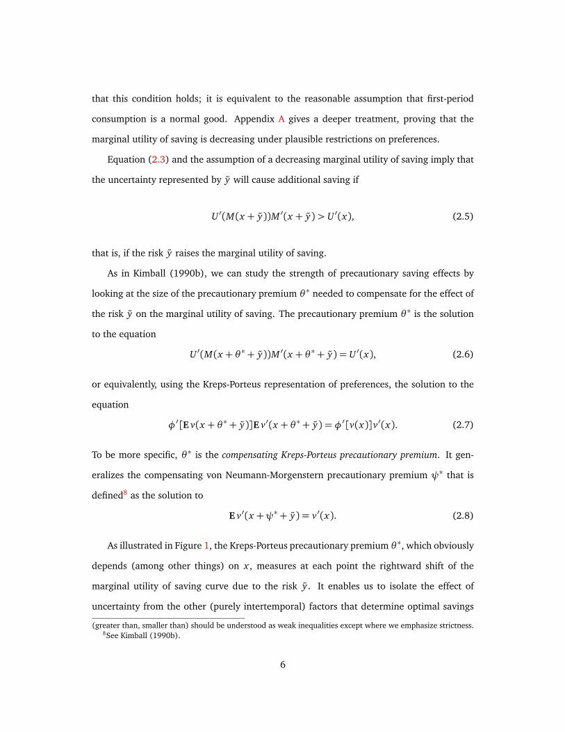
As illustrated in Figure 1, the Kreps-Porteus precautionary premium θ ∗, which obviously
depends (among other things) on x , measures at each point the rightward shift of the
marginal utility of saving curve due to the risk y . It enables us to isolate the effect of
uncertainty from the other (purely intertemporal) factors that determine optimal savings
(greater than, smaller than) should be understood as weak inequalities except where we emphasize strictness.8See Kimball (1990b).
6

x0 x0
θ ∗(x0)
u′(w − x)
U ′[M(x + y)]M ′(x + y)
U ′(x)
Figure 1: Precautionary saving
under certainty.
Also, as shown in Kimball (1990b), Appendix B, the compensating precautionary pre-
mium θ ∗ is the rightward shift of the consumption function due to y . The closely related
equivalent precautionary premium9 θ gives the leftward shift of the consumption function
due to eliminating the risk y . Hence, the extra consumption due to eliminating y , or equiv-
alently the reduced consumption and increased saving due to the presence of y is equal to∫ w
w−θc′(ω, 0)dω, where c′(w, 0) is the marginal propensity to consume out of wealth in the
absence of uncertainty. If the marginal propensity to consume is constant in the absence of
uncertainty, the increment to saving from y will be directly proportional to the size of the
equivalent precautionary premium.
9The equivalent Kreps-Porteus precautionary premium is the solution to the equation U ′[M(x + y)]M ′(x +
y) = U ′[x − θ (x)] according to the Selden representation of preferences, or to φ′[E v(x + y)]E v′(x + y) =
φ′[v(x−θ )]v′(x−θ ) according to the Kreps-Porteus representation. Kimball (1990b), Appendix A shows thatcomparative statics of the compensating precautionary premium carry over to the equivalent precautionarypremium.
7

3 Small risks: a local measure of the strength of the precaution-
ary saving motive
In appendix B, we prove that, for a small risk y with mean zero and variance σ2,
θ ∗(x) = a(x)[1+ s(x)ǫ(x)]σ2
2+ o(σ2), (3.1)
where
s(x) =−U ′(x)
xU ′′(x)(3.2)
denotes the elasticity of intertemporal substitution for the second period utility function
U(x),10 o(σ2) collects terms going to zero faster than σ2, a(x) is the absolute risk aversion
of v defined in (1.2), and ǫ(x) denotes the elasticity of absolute risk tolerance defined in
(1.5).
Therefore, the local counterpart for Kreps-Porteus preferences to the concept of absolute
prudence defined for intertemporal expected utility preferences by Kimball (1990b) is
a(x)[1+ s(x)ǫ(x)].
Similarly, the local counterpart for Kreps-Porteus preferences to relative prudence is
P (x) = γ(x)[1+ s(x)ǫ(x)], (3.3)
where γ(x) = xa(x) is relative risk aversion as above. Therefore, in the more general
framework of Kreps-Porteus preferences, the strength of the precautionary saving motive is
determined both by attitudes towards risk and attitudes towards intertemporal substitution.
Three important special cases should be noted:
10In our definition, the elasticity of intertemporal substitution s(x) is therefore the elasticity of the ratio ofconsumption between periods to the gross real interest rate holding first-period consumption constant.
8
• For intertemporal expected utility maximization, s(x) = 1/γ(x), so that P (x) =
γ(x) + ǫ(x)—which is the expression given in (1.3).
• For constant relative risk aversion, γ(x) = γ and ǫ(x) = 1, so thatP (x) = γ[1+s(x)].
• For constant relative risk aversion γ(x) = γ, and constant (but in general distinct)
elasticity of intertemporal substitution11 s(x) = s, and P (x) = γ[1+ s].
From (3.3), the local condition for positive precautionary saving is simply
ǫ(x)≥ −1
s(x), (3.4)
or, by calculating ǫ(x) from (1.5) and moving one piece to the right-hand side of the
equation:−x v′′′(x)
v′′(x)≥ γ(x)−ρ(x), (3.5)
where
ρ(x) = 1/s(x)
denotes the resistance to intertemporal substitution. The right-hand side of (3.5) is zero un-
der intertemporal expected utility maximization, in which case (3.5) reduces to the familiar
condition v′′′(x)≥ 0.
Intriguingly, equation (3.5) shows that when one departs from intertemporal expected
utility maximization, quadratic risk preferences do not in general lead to the absence of
precautionary saving effects that goes under the name of “certainty equivalence.”
Though the local measure P (x) cannot be used directly to establish global results,
equation (3.1) does suggests several principles which are valid globally, as the next section
shows. First, if one holds the outer intertemporal utility function U fixed, a change in risk
preferences v which raises both risk aversion and its rate of decline tends to strengthen
the precautionary saving motive. Second, decreasing absolute risk aversion (which implies
11 This special case characterizes the framework used by Selden (1979).
9
ǫ(x) ≥ 0) guarantees that the precautionary saving motive is stronger than risk aversion.
Third, if one holds risk preferences constant, raising the elasticity of intertemporal substitu-
tion s(x) and lowering the resistance to intertemporal substitution ρ(x) = 1/s(x), widens
the gap between the strength of the precautionary saving motive and risk aversion. In par-
ticular, when absolute risk aversion is decreasing, lowering the resistance to intertemporal
substitution from the intertemporal utility maximizing level, so that ρ(x) falls below γ(x),
makes the precautionary saving motive stronger than it is under intertemporal expected
utility maximization. Conversely, a resistance to intertemporal substitution ρ(x) greater
than relative risk aversion γ(x) makes the precautionary saving motive weaker than under
intertemporal expected utility maximization.12
4 Large risks
4.1 Precautionary saving and decreasing absolute risk aversion
In the case of intertemporal expected utility maximization, Drèze and Modigliani (1972)
prove that decreasing absolute risk aversion leads to a precautionary saving motive stronger
than risk aversion. Kimball (1997) shows that there is a fundamental economic logic behind
this result: decreasing absolute risk aversion means that greater saving makes it more
desirable to take on a compensated risk. But the other side of such a complementarity
between saving and a compensated risk is that a compensated risk makes saving more
attractive.
This argument follows not from any model-specific features but rather from the logic
of complementarity itself. To understand this claim, consider an arbitrary, concave indirect
utility function of saving and the presence or absence of a compensated risk: J(x ,λ), where
12There are several further minor but interesting propositions suggested by (3.1) which are valid globally.First, constant absolute risk aversion implies that ε = 0, so that the precautionary saving motive and risk aver-sion are of exactly equal strength, regardless of intertemporal substitution. Second, two easy sets of sufficientconditions for a positive precautionary saving motive that are valid globally are (a) decreasing absolute riskaversion or (b) v′′′(·)≥ 0 and ρ(x)≥ γ(x).
10

x is saving and λ is 1 in the presence of the compensated risk y + π∗ and zero in its
absence.13 The definition of a compensated risk insures that
J(x , 1)− J(x , 0) = 0,
i.e., that the consumer is indifferent to the presence or absence of the risk y +π∗.
In the most fundamental sense (i.e., independently of any particular model), the prop-
erty of decreasing absolute risk aversion means that a risk to which an agent is indifferent
at one level of saved wealth will become desirable at a slightly higher level of saved wealth.
Thus,∂
∂ x[J(x , 1)− J(x , 0)] = Jx(x , 1)− Jx(x , 0)≥ 0
if absolute risk aversion is decreasing. But this implies that if the first-order condition for
optimal saving is satisfied in the absence of the compensated risk—i.e., if Jx(x , 0) = 0, then
Jx(x , 1)≥ 0,
implying that a compensated risk makes the agent want to save more. In other words, the
risk premium needed to compensate the agent for the risk he or she is bearing does not
eliminate the total effect of the (compensated) risk on saving. This is what we mean when
we say that the precautionary saving motive is stronger than risk aversion.14
We now examine more formally how this general logic manifests itself in the specific
framework we are studying.
13In the Kreps-Porteus model, for instance, J(x ,λ) = u(w − x) + U[M(x + λ( y +π∗))]. See equation (4.1)below for a precise definition of the compensating risk premium π∗.
14Note that while a nonnegative precautionary saving motive is equivalent to supermodularity between sav-ing and mean zero risks, U(M(x + δ + ε) + U(M(x))− U(M(x + δ))− U(M(x + ε)) ≥ 0, where δ > 0 andEε = 0, the line of reasoning connecting decreasing absolute risk aversion and a precautionary saving motivestronger than risk aversion uses the more subtle symmetry of a single-crossing property in two arguments thatboth have a zero marginal effect on the objective function at a joint crossing point. Supermodularity betweensaving and y +π∗ typically does not hold, since y +π∗ is likely to be strictly desirable at high levels of x andstrictly undesirable at low levels of x .
11

4.1.1 Intertemporal expected utility maximization: a reminder
Under intertemporal expected utility maximization, decreasing absolute risk aversion im-
plies that if π∗ is the compensating risk premium for y , which satisfies
E v(x +π∗+ y) = v(x), (4.1)
then
E v(x +δ+π∗+ y)≥ v(x +δ) (4.2)
for any δ ≥ 0.15 Equation (4.1) and inequality (4.2) together imply that the derivative of
the left-hand side of (4.2) at δ = 0 must be greater than the derivative of the right-hand
side of (4.2) at δ = 0:
E v′(x +π∗+ y)≥ v′(x). (4.3)
Equation (2.8) defining the compensating von Neumann-Morgenstern precautionary pre-
mium ψ∗ differs from (4.3) only by having ψ∗ in place of π∗ and by holding with equal-
ity. Therefore, since v′ is a decreasing function, ψ∗ ≥ π∗. In words, (4.3) says that a
risk compensated by π∗, so that the agent is indifferent to the combination π∗ + y , still
raises expected marginal utility. Therefore, the von Neumann-Morgenstern precautionary
premium ψ∗— which brings expected marginal utility back down to what it was under
certainty—must be greater than π∗.
4.1.2 Kreps-Porteus preferences
The same economic logic applies to the Kreps-Porteus case. Any property that ensures that
extra saving makes compensated risks more attractive guarantees that extra compensated
risk makes saving more desirable. Formally, decreasing absolute risk aversion guarantees
15In other words, the risk premium π∗ that compensates for the effect of the risk y on utility when wealth isx more than compensates for the effect of risk y when wealth is x +δ.
12

that M ′(·)≥ 1, since differentiating the identity
M(x +π∗(x) + y)≡ x (4.4)
yields
(1+π∗′(x))M ′(x +π∗(x) + y) = 1. (4.5)
Decreasing absolute risk aversion implies that π∗′(x) ≤ 0. (Monotonicity of v implies that
1+π∗′(x)≥ 0.) Thus,
U ′(M(x +π∗+ y))M ′(x +π∗+ y) = U ′(x)M ′(x +π∗+ y)≥ U ′(x), (4.6)
where the equality on the left follows from (4.4),16 and the inequality on the right follows
from M ′(·) ≥ 1. Combined with the assumption of a decreasing marginal utility of saving,
(4.6) implies θ ∗ ≥ π∗. We have thus proved:
Proposition 1 Assuming a decreasing marginal utility of saving, if risk preferences v exhibit
decreasing absolute risk aversion, then the Kreps-Porteus precautionary premium is always
greater than the risk premium (θ ∗ ≥ π∗).
Remark. By reversing the direction of the appropriate inequalities above, one can see that
globally increasing absolute risk aversion guarantees that θ ∗ ≤ π∗, just as globally decreas-
ing absolute risk aversion guarantees that θ ∗ ≥ π∗. If absolute risk aversion is constant, both
inequalities must hold, implying that θ ∗(x) ≡ π∗(x) ≡ constant,17 regardless of the form of
the intertemporal utility function U .
16Note that the risk premium π∗ is the same as it would be under intertemporal expected utility maximiza-tion.
17Weil (1993) exploits the fact that θ ∗(x) ≡ π∗(x) under constant absolute risk aversion to solve a multi-period saving problem with Kreps-Porteus utility.
13

4.1.3 Patent increases in risk
Proposition 1 can be extended to patent increases in risk, which, as defined by Kimball
(1993), are increases in risk for which the risk premium increases with risk aversion, at
least when a utility function with decreasing absolute risk aversion is involved. The set of
patent increases in risk includes increases in the scale of a risk coupled with any change of
location, and the addition of any independent risk, but does not include all mean-preserving
spreads.18
The compensating risk premium Π∗(x) for the difference between two risks Y and y is
defined by
E v(x +Π∗(x) + Y ) = E v(x + y), (4.7)
or equivalently, by
M(x +Π∗(x) + Y ) = M(x + y). (4.8)
If Y is a patently greater risk than y , then decreasing absolute risk aversion guarantees that
Π∗(x) is a decreasing function of x . (Given decreasing absolute risk aversion, reducing x
increases risk aversion and therefore increases Π∗ by the definition of a patently greater
risk.) Differentiating equation (4.8) with respect to x , one finds that
M ′(x + y) = [1+Π∗′(x)]M ′(x +Π∗(x) + Y )
≤ M ′(x +Π∗(x) + Y ), (4.9)
where the inequality on the second line follows from Π∗′(x)≤ 0. In combination, equations
18As noted in Kimball (1993), “. . . the results of Pratt (1988) make it clear that X is patently more riskythan x if X can be obtained from x by adding to x a random variable ν that is positively related to x in thesense of having a distribution conditional on x which improves according to third-order stochastic dominancefor higher realizations of x . This sufficient condition for patently greater risk includes as polar special cases νperfectly correlated with x—which makes the movement from x to X a simple change of location and increasein scale—and ν statistically independent of x .”
14

(4.8) and (4.9) imply that
U ′(M(x +Π∗(x) + Y ))M ′(x +Π∗(x) + Y )≥ U ′(M(x + y))M ′(x + y). (4.10)
Defining the compensating Kreps-Porteus precautionary premium Θ∗(x) for the difference
between the two risks Y and y by
U ′(M(x +Θ∗(x) + Y ))M ′(x +Θ∗(x) + Y ) = U ′(M(x + y))M ′(x + y), (4.11)
a decreasing marginal utility of saving implies that Θ∗(x)≥ Π∗(x).
Proposition 2 (extension of Proposition 1) Assuming a decreasing marginal utility of sav-
ing, if risk preferences v exhibits decreasing absolute risk aversion and Y is patently riskier
than y, then the Kreps-Porteus precautionary premium for the difference between Y and y is
always greater than the risk premium for the difference between Y and y—i.e., Θ∗ ≥ Π∗.
Proof: See above. �
4.2 Comparative statics
We now examine how the strength of the precautionary saving motive is affected by
changes in intertemporal substitution, risk aversion, and wealth.
4.2.1 Intertemporal substitution
Before analyzing the effect of intertemporal substitution on the size of the precautionary
premium in general, it is instructive to examine how departures from intertemporal ex-
pected utility maximization affect the precautionary premium:
Proposition 3 Assuming a decreasing marginal utility of saving for the Kreps-Porteus utility
function u(c1) +φ(E v(c2)), if the von Neumann-Morgenstern precautionary premium ψ∗ is
15

greater than the risk premium π∗ (as it will be if absolute risk aversion is decreasing), then
the Kreps-Porteus precautionary premium θ ∗ ≤ ψ∗ when the function φ(·) is concave, but
θ ∗ ≥ψ∗ when φ(·) is convex. If ψ∗ ≤ π∗ (as it will be if absolute risk aversion is increasing),
then θ ∗ ≥ψ∗ when φ(·) is concave, but θ ∗ ≤ψ∗ when φ(·) is convex.
Proof: Assume first that ψ∗ ≥ π∗ and φ(·) is concave. Then
φ′(E v(x +ψ∗ + y))E v′(x +ψ∗ + y) = φ′(E v(x +ψ∗ + y))v′(x)
≤ φ′(v(x))v′(x). (4.12)
The equality on the first line follows from the definition of ψ∗, and the inequality on the second line follows
from ψ∗ ≥ π∗, the monotonicity of v and the concavity of φ(·), which makes φ′(·) a decreasing function.
Together with a decreasing marginal utility of saving, (4.12) implies that
θ ∗ ≤ψ∗. (4.13)
Either the convexity of φ(·) or the inequality ψ∗ ≤ π∗ would reverse the direction of the inequalities in both
(4.12) and (4.13), while convexity of φ(·) and ψ∗ ≤ π∗ together leave the direction of the inequalities un-
changed. �
The results of Proposition 3 are summarized in Table 1.19
φ concave φ convex
(ρ > γ) (ρ < γ)
v DARA π∗ ≤ θ ∗ ≤ψ∗ π∗ ≤ψ∗ ≤ θ ∗
v IARA ψ∗ ≤ θ ∗ ≤ π∗ θ ∗ ≤ψ∗ ≤ π∗
Table 1: Summary of Proposition 3
Concavity of φ brings the Kreps-Porteus precautionary premium θ ∗ closer than the von
Neumann-Morgenstern precautionary premium ψ∗ to the risk premium π∗. Convexity of
φ pushes θ ∗ further than ψ∗ from π∗. For example, for quadratic utility—which exhibits
19 The comparisons between π∗ and θ ∗ follow from Proposition 1.
16
IARA and for which ψ∗ = 0— the precautionary premium θ ∗ is positive if φ is concave and
negative if φ is convex.
Since concavity of φ is equivalent to the elasticity of intertemporal substitution s(x)
below relative risk tolerance 1/γ(x), and convexity of φ is equivalent to the elasticity of
intertemporal substitution s(x) above relative risk tolerance 1/γ(x), one can see that the
pattern is one of greater intertemporal substitution increasing the distance between the risk
premium π∗ and the Kreps-Porteus precautionary premium θ ∗.
Proposition 4 indicates that, holding risk preferences fixed, higher intertemporal sub-
stitution (or equivalently, a lower resistance to intertemporal substitution) leads quite gen-
erally to a Kreps-Porteus precautionary premium that is further from the risk premium:
Proposition 4 If, for two Kreps-Porteus utility functions ui(c1)+Ui(M(c2)), i = 1,2, with the
same risk preferences,
(a) the optimal amount of saving under certainty is the same,
(b) the marginal utility of saving is decreasing for both utility functions, and
(c) U2 has greater resistance to intertemporal substitution than U1—that is,−U ′′2 (x)
U ′2(x)≥−U ′′1 (x)
U ′1(x)
for all x,
then |θ ∗2 − π∗| ≤ |θ ∗1 − π
∗|, where θi is the Kreps-Porteus precautionary premium for utility
function i and π∗ is the risk premium for both utility functions. Also, θ ∗2 − π∗ and θ ∗1 − π
∗
have the same sign.
Proof: See Appendix C. �
The conditions of the proof apply, for instance, when
ui(c1) + Ui(M(c2)) =c
1−ρi
1
1−ρi
+[M(c2)]
1−ρi
1−ρi
17

with ρi > 0, i.e., when the elasticity of intertemporal substitution is constant, and the sub-
jective discount rate equals the interest rate (which we have assumed to be zero). In that
case, the optimal amount of saving under certainty does not depend on ρi , as there is per-
fect consumption smoothing (condition a of proposition 4). Mild conditions on M , spelled
out in Appendix A, guarantee that the marginal utility of saving is decreasing (condition
b of proposition 4). The utility function U2 displays greater resistance to intertemporal
substitution than U1 if ρ2 > ρ1 (condition c).
Remark. Using the machinery for the proof of Proposition 4, Appendix C also provides
graphical intuition for why intertemporal substitution, risk aversion and the rate of decline
of risk aversion matter in the way they do for the strength of the precautionary saving
motive.
4.2.2 Risk aversion
Next, we examine how the strength of the precautionary saving motive is affected by
changes in risk aversion.
Given two inner interpossibility functions v1 and v2, define
Mi(x + y) = v−1i (E vi(x + y)) (4.14)
for i = 1,2, and define θ ∗1 and θ ∗2 by appropriately subscripted versions of (2.6). Then one
can state the following lemma:
Lemma 1 Assuming a decreasing marginal utility of saving and a concave intertemporal util-
ity function U that is held fixed when risk preferences are altered, if
U ′(M2(ξ+ y))M ′2(ξ+ y)≥ U ′(M1(ξ+ y))M ′1(ξ+ y)
for all ξ, then θ ∗2 (x)≥ θ∗1 (x).
18

Proof: Letting ξ= x + θ ∗1 (x),
U ′(M2(x+θ∗1 (x) + y))M ′2(x + θ
∗1 (x) + y)
≥ U ′(M1(x + θ∗1 (x) + y))M ′1(x + θ
∗1 (x) + y)
= U ′(x). (4.15)
Thus, the Kreps-Porteus precautionary premium θ ∗1 for the first set of risk preferences is insufficient under the
second set of risk preferences to bring the marginal utility of saving back down to U ′(x). By the assumption of
a decreasing marginal utility of saving, this means that θ ∗2 must be greater than θ ∗1 to bring the marginal utility
of saving all the way back down to U ′(x). �
This lemma has an obvious corollary:
Corollary 1 Assuming a decreasing marginal utility of saving and a concave outer intertem-
poral utility function U that is held fixed when risk preferences are altered, if M2(ξ+ y) ≤
M1(ξ+ y) and M ′2(ξ+ y)≥ M ′1(ξ+ y) at ξ= x + θ ∗1 (x), then θ ∗2 (x)≥ θ∗1 (x).
The corollary is less helpful than one might hope because it is not easy to find suitable
conditions to guarantee that M ′2 ≥ M ′1. To see why it is not easy, consider the case of a two-
point risk and two different interpossibility functions that both go from infinite positive risk
aversion at zero, to zero risk aversion at infinity. Then, at zero, both certainty equivalents
will converge to the lower outcome of the two-point risk, while at infinity, both certainty
equivalents will converge to the mean value of the two-point risk. Since the certainty
equivalents start and end at the same values, unless M2 and M1 are identical functions the
difference in their slope, M ′2 − M ′1, must change sign at least once, so one cannot always
have M ′2 ≥ M ′1. There is, though, at least one case in which it is easy to establish that
M ′2 ≥ M ′1: when v1 has increasing (or constant) absolute risk aversion, so that M ′1 ≤ 1,
while v2 has decreasing (or constant) absolute risk aversion, so that M ′2 ≥ 1. This result is
equivalent to Proposition 3 and Table 1.
We do get clear results covering one important class of utility functions: the constant
19

elasticity of intertemporal substitution, constant relative risk aversion (CEIS-CRRA) class.
The next proposition focuses on the effect of risk aversion on the strength of the pre-
cautionary saving motive. Within the CEIS-CRRA class, it takes care of the case where the
resistance to intertemporal substitution (the reciprocal of the elasticity of intertemporal
substitution) is greater than risk aversion.
Proposition 5 Suppose two Kreps-Porteus utility functions share the same intertemporal func-
tion U but have different inner interpossibility functions v1 and v2. If
(a) the resistance to intertemporal substitution is greater than the risk aversion of v1 (that is,
U is an increasing, concave transformation of v1),
(b) v2 is globally more risk averse than v1 (that is, −v′′2 (x)/v′2(x) ≥ −v′′1 (x)/v
′1(x) for all
x),
(c) v2 is globally more prudent than v1 (that is, −v′′′2 (x)/v′′2 (x)≥ −v′′′1 (x)/v
′′1 (x) for all x),
(d) v2 has decreasing absolute risk aversion, and
(e) both Kreps-Porteus utility functions have a decreasing marginal utility of saving,
then the Kreps-Porteus precautionary premium given v2 is greater than the Kreps-Porteus pre-
cautionary premium given v1.
Proof: See Appendix D. �
Within the CEIS-CRRA class, all the conditions of Proposition 5 are satisfied when v2 is
more risk averse than v1 and U also has greater curvature than v1.
A second proposition about the effect of greater risk aversion on the strength of the
precautionary saving motive takes care of the case within the CEIS-CRRA class where the
elasticity of intertemporal substitution is less than one:
Proposition 6 Suppose two Kreps-Porteus utility functions share the same outer intertemporal
function U but have different inner interpossibility functions v1 and v2. If
20
(a) the resistance to intertemporal substitution is greater than 1 (that is, U(x) is an increas-
ing, concave transformation of ln(x)),
(b) v2 is globally more risk averse than v1 (that is, −v′′2 (c)/v′2(c)≥ −v′′1 (c)/v
′1(c) for all c),
(c) v1 has constant or increasing relative risk aversion
(d) v2 has constant or decreasing relative risk aversion, and
(e) both Kreps-Porteus utility functions have a decreasing marginal utility of saving,
then the Kreps-Porteus precautionary premium given v2 is greater than the Kreps-Porteus pre-
cautionary premium given v1.
Proof: See Appendix E. �
Within the CEIS-CRRA class, all the conditions of Proposition 6 are satisfied when v2
is more risk averse than v1 and the elasticity of intertemporal substitution is less than or
equal to one.
Empirically, there is strong evidence that the elasticity of intertemporal substitution is
no larger than one, so this proposition takes care of all the empirically relevant cases within
the CEIS-CRRA class.20
In Proposition 6, as in Proposition 5, an assumption is needed that insures that the
absolute risk aversion of v2 decreases fast enough relative to the absolute risk aversion
of v1. In Proposition 5, the assumption of greater prudence for v2 plays that role. In
Proposition 6, the assumption that v2 has constant or decreasing relative risk aversion,
while v1 has constant or increasing relative risk aversion plays that role.
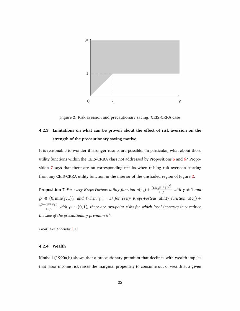
Together, Propositions 5 and 6 guarantee that if a CEIS-CRRA utility function has values
of γ and ρ in the shaded region of Figure 2, while the second function has parameter values
directly to the right (whether or not in the shaded region), the precautionary premium will
be greater for the second utility function.
20See for example Hall (1988) and Barsky, Juster, Kimball, and Shapiro (1997).
21
γ
ρ
0 1
1
Figure 2: Risk aversion and precautionary saving: CEIS-CRRA case
4.2.3 Limitations on what can be proven about the effect of risk aversion on the
strength of the precautionary saving motive
It is reasonable to wonder if stronger results are possible. In particular, what about those
utility functions within the CEIS-CRRA class not addressed by Propositions 5 and 6? Propo-
sition 7 says that there are no corresponding results when raising risk aversion starting
from any CEIS-CRRA utility function in the interior of the unshaded region of Figure 2.
Proposition 7 For every Kreps-Porteus utility function u(c1) +[E (c2)
1−γ]1−ρ1−γ
1−ρwith γ 6= 1 and
ρ ∈ (0,min{γ, 1}), and (when γ = 1) for every Kreps-Porteus utility function u(c1) +
e(1−ρ)[E ln(c2)]
1−ρwith ρ ∈ (0,1), there are two-point risks for which local increases in γ reduce
the size of the precautionary premium θ ∗.
Proof: See Appendix F. �
4.2.4 Wealth
Kimball (1990a,b) shows that a precautionary premium that declines with wealth implies
that labor income risk raises the marginal propensity to consume out of wealth at a given
22

level of first-period consumption. As can be seen from studying Figure 1, this connection
between a decreasing precautionary premium and the marginal propensity to consume
holds for Kreps-Porteus preferences as well. In the two-period case with intertemporal ex-
pected utility maximization, decreasing absolute prudence is necessary and sufficient for a
decreasing precautionary premium. Section 3 points to a necessary condition for a decreas-
ing precautionary premium that is sufficient only for small risks: d
d xa(x)[1+s(x)ε(x)]≤ 0.
This subsection identifies conditions for a decreasing precautionary premium that are suf-
ficient both for both small and large risks.
Given a decreasing marginal utility of saving, define Q(w) by the identity
U ′(Q(w))≡ U ′(M(w))M ′(w). (4.16)
Then
Q(x + θ ∗(x) + y)≡ x ,
and
[1+ θ ∗′
(x)]Q′(x + θ ∗(x) + y) = 1.
As a consequence, the precautionary premium is decreasing in x if and only if Q′(w) ≥ 1
with w = x + θ ∗(x , y) + y .
Differentiation of (4.16) yields
U ′′(Q(w))Q′(w) = U ′′(M(w))[M ′(w)]2+ U ′(M(w))M ′′(w).
Changing signs and dividing by the square of (4.16), we find
�
−U ′′(Q)
[U ′(Q)]2
�
Q′ =
�
−U ′′(M)
[U ′(M)]2
�
+
�
1
U ′(M)
��
−M ′′
[M ′]2
�
, (4.17)
23
with the argument w suppressed for clarity.
Appendix A shows, following Hardy, Littlewood, and Polya (1952, pp. 85-88), that con-
cave absolute risk tolerance of v is sufficient to guarantee that the certainty equivalent
function M is concave. Since CRRA, exponential and quadratic utility—with or without
a shifted origin—yield linear absolute risk tolerance, weakly concave absolute risk toler-
ance holds for an important set of inner interpossibility functions v. This result makes the
following proposition very useful:
Proposition 8 Given the Kreps-Porteus utility function u(c1) + U(v−1(E v(c2))) with U and
v increasing and concave, if
(a) absolute risk aversion is decreasing,
(b) the certainty-equivalent function M for the inner interpossibility function v is concave,
and
(c) −U ′′(x)
[U ′(x)]2is (weakly) increasing,
then the precautionary premium is decreasing in wealth.
Proof: First, as shown in Appendix A, if both M(w) and U(x) are increasing and concave, then the marginal
utility of saving is decreasing. Second, decreasing absolute risk aversion guarantees not only that M ′ ≥ 1, but
also, by (4.16), that Q(w)≤ M(w). Since − U ′′(x)
[U ′(x)]2is increasing,
−U ′′(Q)
[U ′(Q)]2≤ −
U ′′(M)
[U ′(M)]2.
Therefore,
�
−U ′′(Q)
[U ′(Q)]2
�
≤
�
−U ′′(M)
[U ′(M)]2
�
+
�
1
U ′(M)
��
−M ′′
[M ′]2
�
,
implying by (4.17) that Q′ ≥ 1. �
Remark. If the elasticity of intertemporal substitution is constant, condition (c), which
requires − U ′′(x)
[U ′(x)]2to be increasing, is equivalent to ρ ≥ 1, or to an elasticity of intertem-
24

poral substitution s less than or equal to 1. More generally, this condition is equivalent to
s′(x)≤1−s(x)
x, where s(x) = −
U ′(x)
xU ′′(x).
For the effect of greater risk aversion on the precautionary premium, Section 4.2.2
provides results that cover the CEIS-CRRA case not only for ρ ≥ 1, but also for ρ ≥ γ.
We can do the same for the effect of wealth on the precautionary premium. Proposition 9
shows that if the precautionary premium is decreasing for a utility function at any point in
Figure 2, the precautionary premium will also be decreasing at any utility function directly
above it on Figure 2, up to the point where ρ = 1. Proposition 10 combines this result
with the fact that the precautionary premium is decreasing for the CRRA intertemporal
expected utility case ρ = γ to demonstrate that within the CEIS-CRRA class, ρ ≥ γ is
enough to guarantee a decreasing precautionary premium, even if ρ < 1.
Proposition 9 Suppose two Kreps-Porteus utility functions share the same inner interpossibil-
ity function v but have different increasing, concave intertemporal functions U1 and U2 and
associated precautionary certainty equivalence functions Q1(w) and Q2(w). If
(a) v has decreasing absolute risk aversion,
(b) Q′1(w)≥ 1 so that the precautionary premium for the first utility function is decreasing,
(c) −U ′′2 (x)
U ′2(x)≥ −
U ′′1 (x)
U ′1(x), or equivalently U2 has a greater resistance to intertemporal substitution
than U1,
(d) 2U ′′2 (x)
U ′2(x)−
U ′′′2 (x)
U ′′2 (x)≤ 2
U ′′1 (x)
U ′1(x)−
U ′′′1 (x)
U ′′1 (x), and
(e) either 2U ′′1 (x)
U ′1(x)−
U ′′′1 (x)
U ′′1 (x)or 2
U ′′2 (x)
U ′2(x)−
U ′′′2 (x)
U ′′2 (x)is a decreasing function,
then Q′2(w)≥ 1, so that the precautionary premium for the second utility function is decreasing
at the corresponding point.
Proof: See Appendix G. �
25

Remark. When the elasticity of intertemporal substitution s and its reciprocal ρ are con-
stant, condition (c) boils down to ρ2
x≥
ρ1
x, condition (d) boils down to 1−ρ2
x≤
1−ρ1
x,
and condition (e) boils down to 1−ρi
xbeing a decreasing function for one of the functions,
which is guaranteed if either ρi ≤ 1. Thus, for the CEIS-CRRA utility functions, Proposition
9 applies in exactly the region where Proposition 8 cannot be used.
The foregoing proposition has an obvious corollary. Set U1(x) = v(x) and denote
U2(x) = U(x):
Proposition 10 (corollary to Proposition 9) Suppose a Kreps-Porteus utility function satis-
fies the conditions
(a) the inner interpossibility function v is increasing, concave, has decreasing absolute risk
aversion and decreasing absolute prudence,
(b) −U ′′(x)
U ′(x)≥ −
v′′(x)
v′(x), or equivalently ρ(x)≥ γ(x),
(c) 2 U ′′(x)
U ′(x)−
U ′′′(x)
U ′′(x)≤ 2 v′′(x)
v′(x)−
v′′′(x)
v′′(x), and
(d) either 2 v′′(x)
v′(x)−
v′′′(x)
v′′(x)or 2 U ′′(x)
U ′(x)−
U ′′′(x)
U ′′(x)is a decreasing function,
then the precautionary premium θ ∗(x) is decreasing.
The condition that v has decreasing absolute prudence is needed to guarantee that Q′1 ≥ 1
with U1 = v.
Within the CEIS-CRRA class, the conditions of Proposition 10 are all guaranteed when
1 > ρ > γ. Propositions 8 and 10 taken together thus establish that the precautionary pre-
mium is decreasing for large risks for any set of parameters in the shaded region of Figure
2. This is the same region in which greater risk aversion increases the size of the precau-
tionary premium. Conversely, Proposition 11 demonstrates that one cannot guarantee a
decreasing precautionary premium for any of the utility functions in the interior of the un-
shaded region in Figure 2. Thus, the utility functions in the unshaded region—those with
26
a resistance to intertemporal substitution below one and below relative risk aversion—are
badly behaved in relation to both the effect of risk aversion and the effect of wealth on the
strength of the precautionary saving motive:
Proposition 11 For every Kreps-Porteus utility function u(c1) +[E (c
1−γ2 )]
1−ρ1−γ
1−ρwith γ 6= 1
and ρ ∈ (0,min{γ, 1}), and (when γ = 1) for every Kreps-Porteus utility function u(c1) +
e(1−ρ)[E ln(c2)]
1−ρwith ρ ∈ (0,1), there are two-point risks for which increases in wealth raise the
size of the precautionary premium θ ∗.
Proof: See Appendix H. �
5 Conclusion
We have made considerable progress in understanding the determinants of the strength of
the precautionary saving motive under Kreps-Porteus preferences in the two-period case.
Perhaps one of the more surprising results is that greater risk aversion tends to increase
the strength of the precautionary saving motive, while greater resistance to intertemporal
substitution reduces the strength of the precautionary saving motive in the typical case
of decreasing absolute risk aversion. Thus, distinguishing between risk aversion and the
resistance to intertemporal substitution is very important in discussing the determinants
of the strength of the precautionary saving motive, since these two parameters—which
are forced to be equal under intertemporal expected utility maximization—have opposite
effects when allowed to vary separately.
Our results also bear on judgments about the likely empirical magnitude of the precau-
tionary saving motive. Remember that we show in Section 3 that, for preferences exhibiting
a constant elasticity of intertemporal substitution and constant relative risk aversion, the
local measure (in relative terms) of the strength of the precautionary saving motive is
P = γ(1+ s) = γ(1+ρ−1),
27

γ= 2 γ= 6 γ= 18ρ = 2 3 9 27ρ = 6 2.33 7 21ρ = 18 2.11 6.33 19
Table 2: The local coefficient of relative prudence P = γ(1 + ρ−1) for isoelastic Kreps-Porteus preferences
where γ is the coefficient of relative risk aversion, s is the elasticity of intertemporal substi-
tution, and ρ = 1/s is the resistance to intertemporal substitution.
To give some idea of what this formula means in practice, Table 2 shows the implied
value of the coefficient of relative prudence,P , for γ and ρ both ranging over the three rep-
resentative “low,” “medium,” and “high” values 2, 6 and 18. The words “low,” “medium,”
and “high,” are in quotation marks because the values of both γ and ρ and what values
would count as “low,” “medium” and “high,” in relation to the data are hugely contro-
versial. For instance, economist A might find γ = 2 intuitively reasonable, while being
convinced by consumption Euler equation evidence like that of Hall (1988) that the elas-
ticity of intertemporal substitution s is very small, with s about .055 and thus ρ = 18. By
contrast, economist B might find the value ρ = 2, and the higher implied s = .5, intuitively
more reasonable in relation to what is needed to explain business cycles, but might be con-
vinced by the evidence behind the equity premium puzzle that relative risk aversion should
be at least γ= 18.
If they do not know how to relax the von Neumann-Morgenstern restriction ρ = γ,
these economists with quite divergent views and data about risk aversion and intertempo-
ral substitution might be compelled to compromise on some intermediate value ρ = γ = 6
(taken here for computational simplicity to be the geometric mean of 2 and 18 for both γ
and ρ). This would lead them to agree on a precautionary saving motive strength given
by the relative prudence of 7. This agreement is artificial as, freed by Kreps-Porteus pref-
erences from the restriction ρ = γ, economists A and B would strongly disagree about the
strength of the precautionary saving motive. Economist A would expect a very strong pre-
28
cautionary saving motive with P = 27, while Economist B would expect a much weaker
precautionary saving motive with P = 2.11. In addition, they also would differ widely on
the implied magnitude of the equilibrium equity premium and real interest rate implied by
their model.21
The dramatic quantitative differences illustrated in this example underline the impor-
tance of refining the empirical evidence for the magnitude of risk aversion, and of obtain-
ing distinct estimates of the resistance to intertemporal substitution.22 Kreps-Porteus pref-
erences provide the conceptual foundation of this further empirical research program. In
turn, understanding the precautionary saving effects of Kreps-Porteus preferences is central
to a sound theoretical and empirical understanding of consumption and saving behavior.
21See, for instance, the computations in ?.22One of the key practical implications of distinguishing between risk aversion and the resistance to in-
tertemporal substitution is that, without the restriction that they be equal, there is only half as much empiricalevidence on the value of each as one might otherwise think.
29
Appendix A Conditions guaranteeing a decreasing marginal
utility of saving
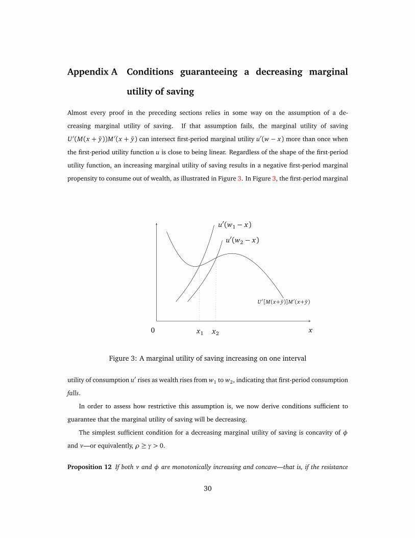
Almost every proof in the preceding sections relies in some way on the assumption of a de-
creasing marginal utility of saving. If that assumption fails, the marginal utility of saving
U ′(M(x + y))M ′(x + y) can intersect first-period marginal utility u′(w − x) more than once when
the first-period utility function u is close to being linear. Regardless of the shape of the first-period
utility function, an increasing marginal utility of saving results in a negative first-period marginal
propensity to consume out of wealth, as illustrated in Figure 3. In Figure 3, the first-period marginal
x0 x1
u′(w1− x)
u′(w2− x)
x2
U ′[M(x+ y)]M ′(x+ y)
Figure 3: A marginal utility of saving increasing on one interval
utility of consumption u′ rises as wealth rises from w1 to w2, indicating that first-period consumption
falls.
In order to assess how restrictive this assumption is, we now derive conditions sufficient to
guarantee that the marginal utility of saving will be decreasing.
The simplest sufficient condition for a decreasing marginal utility of saving is concavity of φ
and v—or equivalently, ρ ≥ γ > 0.
Proposition 12 If both v and φ are monotonically increasing and concave—that is, if the resistance
30

to intertemporal substitution is greater than risk aversion, which in turn is positive—then the marginal
utility of saving is decreasing.
Proof: Concavity of both v and φ guarantees that both factors of the Kreps-Porteus representation of the
marginal utility of saving, φ′(E v(x + y))E v′(x + y), decrease as x increases. �
Alternatively, concavity of both the outer intertemporal function U and of the certainty equiva-
lent function M is enough to guarantee a decreasing marginal utility of saving:
Proposition 13 If both the outer intertemporal utility function U and the certainty equivalent function
M(x + y) are increasing and concave in x, then the marginal utility of saving is decreasing.
Proof: Concavity of both U and M guarantees that both factors of the Selden representation of the marginal
utility of saving, U ′(M(x + y))M ′(x + y), decrease as x increases. �
This result becomes very useful in conjunction with Proposition 14 below (adapted from
Hardy, Littlewood, and Polya’s classic book Inequalities) that the certainty equivalent function M is
always concave for risk preference function function v with concave absolute risk tolerance, which
includes any v in the hyperbolic absolute risk aversion class, including quadratic, exponential, linear,
and constant relative risk aversion utility functions, which all have linear absolute risk tolerance.23
Proposition 14 If v′(x) > 0, v′′(x) < 0, and −v′(x)
v′′(x)is a concave function of x, then M(ξ+ y) =
v−1(E v(ξ+ y)) is a concave function of ξ.
Proof: As noted above, this proof is adapted from Hardy, Littlewood, and Polya (1952). Write ξ + y = w.
Differentiating the identity
23Utility functions in the hyperbolic absolute risk aversion class are those that can be expressed in the form
v(x) =γ
1−γ
§�
x−b
γ
�1−γ− 1ª
together with the logarithmic limit as γ→ 1 and the exponential limit as γ→∞
with b
γ→−a. As pointed out by an anonymous referee, outside of the constant relative risk aversion class, an
increasing concave utility function must either have a subsistence level of consumption or strictly increasingrelative risk aversion above a certain level in order to have globally concave absolute risk tolerance. Wedo not view either a subsistence level of consumption or some level of increasing relative risk aversion asinherently unreasonable, but it is good to be aware of this constraint. Suppose t(x) = 1/a(x) is well definedand strictly positive on the strictly positive reals. If t ′(x∗) < 0 for some x∗, then concave t(·) would forcet(x) < 0 for large enough x . Also, t ′(x) ≤ t(x)/x is necessary in order to rule out t(x) < 0 for small x .t ′(x) ≤ t(x)/x is equivalent to (weakly) increasing relative risk aversion. Furthermore, concave t(·) impliesthat if t ′(x∗)< t(x∗)/x∗ for any x∗, then t ′(x)< t(x)/x for all x > x∗ as well. Thus, strictly increasing relativerisk aversion at any point implies strictly increasing relative risk aversion above that point as well.
31
v(M(w))≡ E v(w)
yields
v′(M(w))M ′(w) = E v′(w) (A.1)
and
v′(M(w))M ′′(w) + v′′(M(w))[M ′(w)]2 = E v′′(w). (A.2)
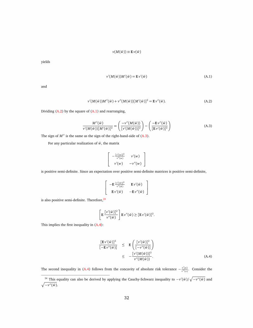
Dividing (A.2) by the square of (A.1) and rearranging,
M ′′(w)
v′(M(w))[M ′(w)]2=
�
−v′′(M(w))
[v′(M(w))]2
�
−
�
−E v′′(w)
[E v′(w)]2
�
(A.3)
The sign of M ′′ is the same as the sign of the right-hand-side of (A.3).
For any particular realization of w, the matrix
−[v′(w)]2
v′′(w)v′(w)
v′(w) −v′′(w)
is positive semi-definite. Since an expectation over positive semi-definite matrices is positive semi-definite,
−E[v′(w)]2
v′′(w)E v′(w)
E v′(w) −E v′′(w)
is also positive semi-definite. Therefore,24
�
E[v′(w)]2
v′′(w)
�
E v′′(w)≥ [E v′(w)]2.
This implies the first inequality in (A.4):
[E v′(w)]2
[−E v′′(w)]≤ E
�
[v′(w)]2
[−v′′(w)]
�
≤ −[v′(M(w))]2
v′′(M(w)). (A.4)
The second inequality in (A.4) follows from the concavity of absolute risk tolerance − v′(x)
v′′(x). Consider the
24 This equality can also be derived by applying the Cauchy-Schwarz inequality to −v′(w)/p
−v′′(w) andp
−v′′(w).
32

function ℓ(z) defined by
ℓ(z)≡ −[v′(v−1(z))]2
v′′(v−1(z)).
Its first derivative is
ℓ′(z)≡v′′′(v−1(z))v′(v−1(z))
[v′′(v−1(z))]2− 2.
For comparison,
∂
∂ x
�
−v′(x)
v′′(x)
�
≡v′′′(x)v′(x)
[v′′(x)]2− 1.
Let z = v(x). Since dz
d x> 0, ℓ′(z) is decreasing if and only if ∂
∂ x
�
−v′(x)
v′′(x)
�
is decreasing. Therefore, ℓ(z) is
concave as a function of z if and only if absolute risk tolerance −v′(x)
v′′(x)is concave as a function of x . In turn,
concavity of ℓ implies
E
�
[v′(w)]2
[−v′′(w)]
�
= Eℓ(v(w))≤ ℓ(E v(w)) = −[v′(M(w))]2
v′′(M(w)).
Inequality (A.4) and equation (A.3) prove that M is concave. �
As for the converse of Proposition 13, a necessary condition on v for U ′(M(x + y))M ′(x + y)
to be decreasing for any concave U (that is, regardless of the size of the resistance to intertemporal
substitution) is for M to be concave.
Only a partial converse is available for Proposition 14. For small risks, the necessary and suffi-
cient condition for M to be concave is for absolute risk aversion−v′′(x)
v′(x)to be convex. (See equation
(B.2).) This is a weaker condition than the concavity of absolute risk tolerance that guarantees con-
cavity of M for large risks, so this does not provide a full converse to Proposition 14. Still, it does
indicate how to find cases where M is convex, which have the potential to violate the assumption
of a decreasing marginal utility of saving for a low enough resistance to intertemporal substitution.
Hardy, Littlewood, and Polya (1952, pp. 85-88) look at a more general result than Proposition 14
(in our notation, they are interested in M( y + xz) being concave in x for any random variable z),
so their converse does not apply.
33
Appendix B Local approximation of section 3
Define the equivalent Kreps-Porteus precautionary premium θ , expressed as a function of x , as the
solution to the equation
U ′[M(x + y)]M ′(x + y) = U ′[x − θ (x)]. (B.1)
It is easiest to find the small-risk approximation for the equivalent Kreps-Porteus precautionary
premium θ first, and then the small risk approximation for the compensating Kreps-Porteus pre-
cautionary premium θ ∗. For a small risk y with mean zero and variance σ2, Pratt (1964) shows
that
M(x + y) = x − a(x)σ2
2+ o(σ2). (B.2)
As long as M ′′(·) is bounded in the neighborhood of x , (B.2) can be differentiated to obtain
M ′(x + y) = 1− a′(x)σ2
2+ o(σ2). (B.3)
Finally, substituting from (B.2) and (B.3) into (B.1), and doing a Taylor expansion of U(x − θ )
around x ,
U ′[M(x + y)]M ′(x + y) = [U ′(x)− U ′′(x)a(x)σ2
2+ o(σ2)] [1− a′(x)
σ2
2+ o(σ2)]
= U ′(x)− [U ′′(x)a(x) + U ′(x)a′(x)]σ2
2+ o(σ2)
= U ′(x)− U ′′(x)θ (x) + o(θ (x)). (B.4)
Using the last equality, we conclude that
θ (x) =
�
a(x) +U ′(x)
U ′′(x)a′(x)
�
σ2
2+ o(σ2). (B.5)
Inspecting (2.6) and (B.1) and then using (B.5) makes it clear that
θ ∗(x) = θ (x + θ ∗(x))
=
�
a(x + θ ∗(x)) +U ′(x + θ ∗(x))
U ′′(x + θ ∗(x))a′(x + θ ∗(x))
�
σ2
2+ o(σ2)
=
�
a(x) +U ′(x)
U ′′(x)a′(x)
�
σ2
2+ o(σ2), (B.6)
34

as long as a′ and U ′
U ′′are continuous at x . Using (3.2), (B.6) can be rewritten as
θ ∗(x) = a(x)[1+ s(x)ǫ(x)]σ2
2+ o(σ2), (B.7)
which establishes (3.1) in the text.
Appendix C Proof of Proposition 4
The optimal amount of saving for the two utility functions is the same under certainty only if there
is an x0 for which
u′i(w − x0) = U ′
i(x0) i = 1,2. (C.1)
Define the normalized marginal utility of saving functions f1 and f2 by
fi(x) =U ′
i(M(x + y))M ′(x + y)
U ′i(x0)
. (C.2)
For either utility function, the normalized marginal utility of saving fi equals 1 when x = x0 +
θ ∗i(x0). Therefore, f1 and f2 can be used to establish comparative statics for the Kreps-Porteus
precautionary premium θ ∗.
Equation (C.1) says that f1 and f2 meet at x = x0 +π∗(x0), since
U ′i(M(x0 +π
∗(x0) + y))M ′(x0 +π∗(x0) + y)
U ′i(x0)
=U ′
i(x0)M ′(x0 +π
∗(x0) + y)
U ′i(x0)
= M ′(x0 +π∗(x0) + y) (C.3)
for i = 1,2. Since the identity M(x +π∗(x) + y)≡ x can be differentiated to obtain
[1+π∗′(x0)]M′(x0 +π
∗(x0) + y) = 1, (C.4)
both f1(x0 +π∗(x0)) and f2(x0 +π
∗(x0)) are greater than 1 if π′(x0) ≤ 0 and both are less than 1
if π∗′(x0)≥ 0.
35

The ratio between f2 and f1 simplifies as follows:
f2(x)
f1(x)=
U ′2(M(x + y))
U ′1(M(x + y))
U ′1(x0)
U ′2(x0). (C.5)
The condition−U ′′2 (x)
U ′2(x)≥−U ′′1 (x)
U ′1(x)implies that the ratio
U ′2(x)
U ′1(x)is a decreasing function of x since
d
d xln
�
U ′2(x)
U ′1(x)
�
=U ′′2 (x)
U ′2(x)−
U ′′1 (x)
U ′1(x)≤ 0. (C.6)
Since M(x + y) is an increasing function of x , this means that f2(x)
f1(x)is a decreasing function of x .
Therefore, f2(x)≥ f1(x) for x ≤ x0 +π∗(x0) and f2(x)≤ f1(x) for x ≥ x0 +π
∗(x0).
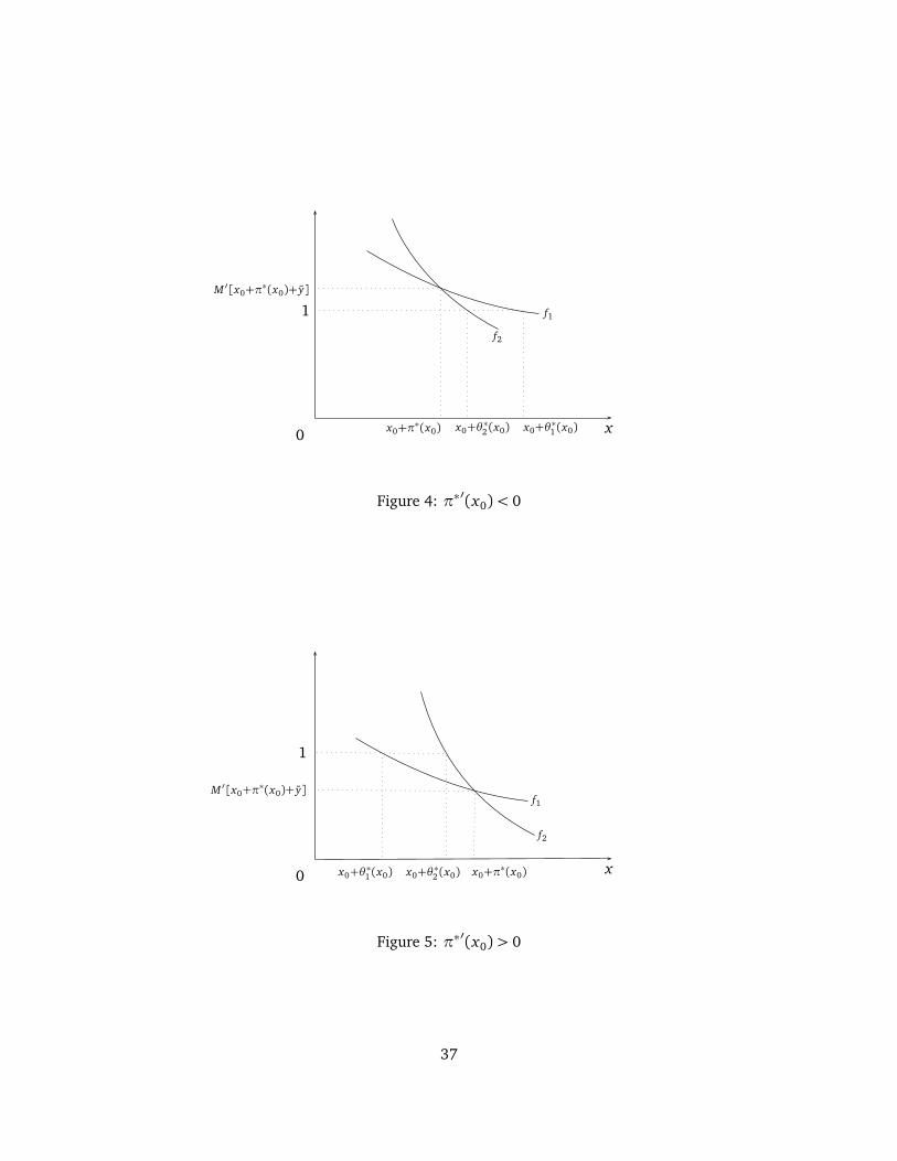
We are now in a position to draw an instructive graph of f1 and f2. Figures 4 and 5 depict the
two main cases. Decreasing marginal utility of saving means that fi is decreasing for both utility
functions. If π∗′(x0) ≤ 0, then f2 and f1 are both above 1 at x = x0 +π∗(x0) and f2 must hit 1 first
as x moves to the right from x0 +π∗(x0) since f2 is below f1 to the right of x0 +π
∗(x0). Therefore
x0 + θ∗2 (x0)≤ x0 + θ
∗1 (x0) and θ ∗2 (x0)≤ θ
∗1 (x0).
If π∗′(x0) ≥ 0, then f2 and f1 are both below 1 at x = x0 + π∗(x0) and f2 must hit 1 first
as x moves to the left from x0 + π∗(x0) since f2 is above f1 to the left of x0 + π
∗(x0). Therefore
x0 + θ∗2 (x0)≥ x0 + θ
∗1 (x0) and θ ∗2 (x0)≥ θ
∗1 (x0).
If one or the other of fi(x) never hits 1, these inequalities remain valid if one writes θ ∗i(x0) =
+∞ when fi(x) > 1 for all x , and θ ∗i(x0) = −∞ when fi(x) < 1 for all x . In all of these cases,
θ1(x0) and θ2(x0) are on the same side of π∗(x0) and |θ ∗2 (x0)−π∗(x0)| ≤ |θ
∗1 (x0)−π
∗(x0)|.
Figures 4 and 5 can be used to illustrate not only the effects of changing the elasticity of in-
tertemporal substitution but also the effects of changing the level and rate of decline of risk aver-
sion. Let us begin by presenting what would be a satisfying intuitive story except that it neglects
one effect. Focusing on the point (x0 + π∗(x0), M ′(x0 + π
∗(x0) + y)) at which the curves f1 and
f2 intersect, increases in risk aversion move this point to the right by increasing π∗, more quickly
declining risk aversion tends to move this point upward by increasing M ′, while increases in the
elasticity of intertemporal substitution swivel the curve describing f counterclockwise around this
point (increases in the resistance to intertemporal substitution swivel the curve clockwise around
this point.) The effects of each change on the strength of the precautionary saving motive can be
seen in the horizontal movement of the intersection with the dashed line f (x) = 1. The message
36
x0 x0+π∗(x0)
1
M ′[x0+π∗(x0)+ y]
x0+θ∗2 (x0) x0+θ
∗1 (x0)
f1
f2
Figure 4: π∗′(x0)< 0
x0 x0+π∗(x0)
1
M ′[x0+π∗(x0)+ y]
x0+θ∗2 (x0)x0+θ
∗1 (x0)
f1
f2
Figure 5: π∗′(x0)> 0
37

of equation (3.3) about the determinants of the strength of the precautionary saving motive under
Kreps-Porteus preferences is clearly confirmed by such an exercise. The fly in the ointment is the
one neglected effect: like the rate of change of risk aversion, changes in the level of risk aversion
can affect M ′ and so move the (x0 +π∗(x0), M ′(x0 +π
∗(x0) + y)) point vertically as well as hori-
zontally. This vertical movement can be either up or down in response to an increase in the level of
risk aversion. The subtleties of section 4.2.2 stem from this complication.
Appendix D Proof of Proposition 5
By Lemma 1, together with the assumption of a decreasing marginal utility of saving, it is enough
to show that U ′(M2)M′2 > U ′(M1)M
′1. Write w = x +θ1+ y . Take the derivative of both sides of the
identity
v(Mi(w))≡ E v(w)
with respect to the addition of nonstochastic constants to get
v′(Mi(w))M′i(w) = E v′(w).
Also define Ni(w) by
v′(Ni(w)) = E v′(w),
so that
M ′i(w) =
v′i(Ni(w))
v′i(Mi(w))
.
Suppressing the arguments for Mi , M ′i
and Ni , we find that
38
U ′(M2)M′2
U ′(M1)M′1
=
U ′(M2)
�
v′2(N2)
v′2(M2)
�
U ′(M1)
�
v′1(N1)
v′1(M1)
�
=
�
U ′(M2)
v′1(M2)
�
�
U ′(M1)
v′1(M1)
�
�
v′2(N2)
v′1(N2)
�
�
v′2(M2)
v′1(M2)
�
¨
v′1(N2)
v′1(N1)
«
≥ 1.
First,
�
U ′(M2)
v′1(M2)
�
�
U ′(M1)
v′1(M1)
� ≥ 1
because resistance to intertemporal substitution greater than risk aversion means that ln(U ′) de-
clines more quickly than ln(v′1), making U ′
v′1a decreasing function, while v2 being more risk averse
than v1 guarantees that M2(w)≤ M1(w). Second,
�
v′2(N2)
v′1(N2)
�
�
v′2(M2)
v′1(M2)
� ≥ 1
because v2 being more risk averse than v1 makesv′2v′1
a decreasing function, and the decreasing
absolute risk aversion of v2 guarantees that N2(w)≤ M2(w). Third,
v′1(N2)
v′1(N1)≥ 1
because v2 being more prudent than v1 guarantees that N2(w)≤ N1(w).
Appendix E Proof of Proposition 6
Using a slightly different rearrangement than in Appendix D,
39
U ′(M2)M′2
U ′(M1)M′1
=
U ′(M2)
�
E v′2(w)
v′2(M2)
�
U ′(M1)
�
E v′1(w)
v′1(M1)
�
=
¨
M2U ′(M2)
M1U ′(M1)
«
�
E wv′1(w)
E v′1(w)
�
�
E wv′2(w)
E v′2(w)
�
�
E wv′2(w)
M2 v′2(M2)
�
�
E wv′1(w)
M1 v′1(M1)
�
≥ 1.
Having the resistance to intertemporal substitution greater than one (or equivalently, the elasticity
of intertemporal substitution less than one) implies that xU ′(x) is a decreasing function. Combined
with v2 being more risk averse than v1, so that M2 ≤ M1, this guarantees that
M2U ′(M2)
M1U ′(M1)≥ 1.
Next, v2 being more risk averse than v1 implies that the function
j(w) =v′1(w)
EW v′1(W )−
v′2(w)
EW v′2(W )
is single-crossing upwards. Let w0 be the crossing point. Then, when W has a distribution that is
identical to, but independent from w, E j(w) = 0 and so
Ew w
�
v′1(w)
EW v′1(W )−
v′2(w)
EW v′2(W )
�
= Ew(w − w0)
�
v′1(w)
EW v′1(W )−
v′2(w)
EW v′2(W )
�
≥ 0.
This implies that
�
E wv′1(w)
E v′1(w)
�
�
E wv′2(w)
E v′2(w)
� ≥ 1.
Finally, defining the functions gi(·) by
x v′i(x)≡ gi(vi(x)), (E.1)
the constant or decreasing relative risk aversion of v2 implies that g2 is convex, while the constant
40

or increasing relative risk aversion of v1 implies that g1 is concave. To show this, differentiate (E.1)
and divide by v′i
to get
1−
�
−x v′′
i(x)
v′i(x)
�
= g ′i(vi(x)). (E.2)
Thus, g ′1 is decreasing (making g1 concave) because relative risk aversion−x v′′1 (x)
v′1(x)is increasing and
g ′2 is increasing (making g2 convex) because−x v′′2 (x)
v′2(x)is decreasing.
The convexity of g2 implies
E wv′2(w) = E g2(v2(w))≥ g2(E v2(w)) = g2(v2(M2(w))) = M2(w)v′(M2(w)).
The concavity of g1 implies
E wv′1(w) = E g1(v1(w))≤ g1(E v1(w)) = g1(v1(M1(w))) = M1(w)v′(M1(w)).
As a result,
�
E wv′2(w)
M2 v′2(M2)
�
�
E wv′1(w)
M1 v′1(M1)
� ≥ 1,
completing the proof.
Appendix F Proof of Proposition 7
Substituting in for M ′ as in the previous appendix, and for the particular functional form used in
Proposition 7, we have
U ′(M(w))M ′(w) = U ′(M(w))E v′(w)
v′(M(w))
= [M(w;γ)]γ−ρE w−γ.
We need to show that the derivative of this expression with respect to γ can be negative. Fortunately,
M(w;γ) is continuously differentiable with respect to γ, even across the γ = 1 boundary. Consider
the two-point risk equal to ε < 1 with probability p and ζ > 1 with probability 1− p. When γ 6= 1,
41

calculate
∂
∂ γln[M(w;γ)γ−ρE w−γ] =
∂
∂ γ
�γ−ρ
1− γln(pε1−γ + (1− p)ζ1−γ) (F.1)
+ ln(pε−γ + (1− p)ζ−γ)�
=1−ρ
(1− γ)2ln(pε1−γ + (1− p)ζ1−γ)
+
�
γ−ρ
1− γ
��
− ln(ε)pε1−γ − ln(ζ)(1− p)ζ1−γ
pε1−γ + (1− p)ζ1−γ
�
+[− ln(ε)pε−γ − ln(ζ)(1− p)ζ−γ]
pε−γ + (1− p)ζ−γ.
For given ε, choose p and ζ so that
pε1−γ = q
and
(1− p)ζ1−γ = 1− q.
That is,
p = qεγ−1 (F.2)
and
ζ =
�
1− q
1− qεγ−1
� 11−γ
. (F.3)
When γ < 1, Equation (F.2) requires ε to be in (q1/(1−γ), 1) to keep p in (0,1). When γ > 1, Equation
(F.2) allows ε to be anywhere in (0,1). As γ→ 1, (F.2) and (F.3) limit into p = q and ζ= ε−q/(1−q).
For all values of γ, the choice in (F.2) and (F.3) makes M(w;γ) = 1. When γ 6= 1, it allows (F.1)
to be written in terms of ε as follows:
42

∂ ln[M(w;γ)γ−ρE w−γ]
∂ γ=
�
γ−ρ
1− γ
�
[−q ln(ε)− (1− q) ln(ζ)]
+[−q ln(ε)ε−1 − (1− q) ln(ζ)ζ−1]
qε−1 + (1− q)ζ−1
(F.4)
Case 1: γ > 1. Choose q ∈�
γ−1γ−ρ
, 1�
. This is possible because ρ < 1 < γ in this case. Consider
the limit as ε→ 0, with p given by (F.2) and ζ given by (F.3). With γ > 1,
limε→0ζ= (1− q)
11−γ ,
and
limε→0
∂ ln[M(w;γ)γ−ρE w−γ]
∂ γ= limε→0
�
qγ−ρ
γ− 1− 1
�
ln(ε)− (1− q) ln(1− q)γ−ρ
(γ− 1)2= −∞.
Therefore, there are values of ε small enough that the derivative of the marginal utility of saving
with respect to γ is negative, which in turn implies a precautionary premium that decreases with γ
over some range.
Case 2: γ < 1. In this case, choose q = .5 and consider the limit as ε→ 2−1/(1−γ) from above.
Then ζ→∞ and
limε→(2−1/(1−γ))
+
∂ ln[M(w;γ)γ−ρE w−γ]
∂ γ= limε→(2−1/(1−γ))
+
(2− γ−ρ) ln(2)
2(1− γ)2−(γ−ρ) ln(ζ)
2(1− γ)=−∞.
Again, this implies that for values of ε close enough above 2−1/(1−γ), the precautionary premium is
decreasing in γ.
Case 3: γ= 1. To deal with this case, let the two-point risk be ε with probability .5 and ζ= ε−1
with probability .5. Then the derivative of the logarithm of the marginal utility of saving is
43
∂
∂ γln[M(w;γ)γ−ρE w−γ] = ln(M(w,γ)) (F.5)
+(γ−ρ)
¨
ln(.5ε1−γ + .5εγ−1)
(1− γ)2
+ln(ε)[εγ−1 − ε1−γ]
(1− γ)[εγ−1 + ε1−γ]
«
+ ln(ε)εγ − ε−γ
εγ + ε−γ
The logarithmic derivative of the marginal utility of saving with respect to γ has a well-defined limit
as γ→ 1 from either side of 1. Using the fact that limγ→1 M(w,γ) = 1 and a messy application of
L’Hopital’s rule, the limit as γ→ 1 of the expression on the right-hand-side of (F.5) is
− ln(ε)
�
1− ε2
1+ ε2
�
− .5(1−ρ)[ln(ε)]2
Clearly, for small enough ε, the marginal utility of saving—and therefore the precautionary
premium—is decreasing in γ on both sides of γ= 1.
Appendix G Proof of Proposition 9
For each utility function Ui , define
hi(λ) =−
�
U ′′i(U ′−1
i(λU ′
i(M(w))))
λ2U ′i(M(w))
�
.
Using the fact that U ′i(Q i) = U ′
i(M)M ′, observe that the counterpart of equation (4.17) for each
utility function can be rewritten, after multiplying through by U ′i(M(w)), as
hi(M′)Q′
i= hi(1)−
M ′′
[M ′]2,
or
hi(M′)(Q′
i− 1) =−
M ′′
[M ′]2− [hi(M
′)− hi(1)]. (G.1)
44

The fact that Ui is increasing and concave guarantees that hi is positive. Therefore, condition (a) in
Proposition 9, Q′1 ≥ 1, is equivalent to the right-hand-side of (G.1) being positive, or
h1(M′)− h1(1)≤−
M ′′
[M ′]2.
We need to find conditions under which this inequality implies that
h2(M′)− h2(1)≤ −
M ′′
[M ′]2(G.2)
as well.
One approach is to try to establish that h′2(λ)≤ 0 and that M ′′ ≤ 0, so that
h2(M′)− h2(1)≤ 0≤ −
M ′′
[M ′]2.
This is exactly what Proposition 8 does. The other approach—the essence of Proposition 9—is to
establish that h′2(λ)≤ h′1(λ) for λ ≥ 1, so that, given M ′ ≥ 1 (a consequence of decreasing absolute
risk aversion),
h2(M′)− h2(1)≤ h1(M
′)− h1(1)≤−M ′′
[M ′]2. (G.3)
Straightforward differentiation yields
h′i(λ) =
1
λ2
¨
2U ′′
i(U ′−1
i(λU ′
i(M)))
λU ′i(M)
−U ′′′
i(U ′−1
i(λU ′
i(M)))
U ′′i(U ′−1
i(λU ′
i(M(w))))
«
.
Defining
qi(λ) = U ′−1i(λU ′
i(M)),
one can write
Q i = qi(M′)
and
45
h′i(λ) =
1
λ2
¨
2U ′′
i(qi(λ))
U ′i(qi(λ))
−U ′′′
i(qi(λ))
U ′′i(qi(λ))
«
. (G.4)
If − U ′′
[U ′]2is increasing, as assumed in Proposition 8, then h′(λ)≤ 0.
The assumption that −U ′′2 (x)
U ′2(x)≥−
U ′′1 (x)
U ′1(x)(condition (c) in Proposition 9) implies that
U ′2(x)
U ′2(M)≥
U ′1(x)
U ′1(M).
for any x ≤ M . Therefore, for any λ≥ 1,
q2(λ) = U ′−12 (λU ′2(M))≥ U ′−1
1 (λU ′1(M)) = q1(λ).
If 2U ′′2 (x)
U ′2(x)−
U ′′′2 (x)
U ′′2 (x)is decreasing (condition (e) in Proposition 9) then
h′2(λ) =1
λ2
¨
2U ′′2 (q2(λ))
U ′2(q2(λ))−
U ′′′2 (q2(λ))
U ′′2 (q2(λ))
«
≤1
λ2
¨
2U ′′2 (q1(λ))
U ′2(q1(λ)−
U ′′′2 (q1(λ))
U ′′2 (q1(λ))
«
≤1
λ2
¨
2U ′′1 (q1(λ))
U ′1(q1(λ)−
U ′′′1 (q1(λ))
U ′′1 (q1(λ))
«
= h′1(λ).
Alternatively, if 2U ′′1 (x)
U ′1(x)−
U ′′′1 (x)
U ′′1 (x)is decreasing (condition (e) in Proposition 9) then
h′2(λ) =1
λ2
¨
2U ′′2 (q2(λ))
U ′2(q2(λ)−
U ′′′2 (q2(λ))
U ′′2 (q2(λ))
«
≤1
λ2
¨
2U ′′1 (q2(λ))
U ′1(q2(λ)−
U ′′′1 (q2(λ))
U ′′1 (q2(λ))
«
≤1
λ2
¨
2U ′′1 (q1(λ))
U ′1(q1(λ)−
U ′′′1 (q1(λ))
U ′′1 (q1(λ))
«
= h′1(λ).
Both cases use condition (d) in Proposition 9: the assumption that 2U ′′2 (x)
U ′2(x)−
U ′′′2 (x)
U ′′2 (x)≤ 2
U ′′1 (x)
U ′1(x)−
U ′′′1 (x)
U ′′1 (x).
46
Appendix H Proof of Proposition 11
Substituting U(x) = x1−ρ
1−ρinto the identity U ′(Q) = U ′(M)M ′ and solving for Q,
Q = M[M ′]−1/ρ.
Differentiating with respect to addition of a nonstochastic constant,
Q′(w) =
�
1−M(w)M ′′(w)
ρ[M ′(w)]2
�
[M ′(w)]1−(1/ρ). (H.1)
Using equation (A.1), we have
M ′ =E v′(w)
v′(M)= MγE w−γ. (H.2)
Differentiating (A.2) and combining the resulting equation with (A.2) itself yields
M M ′′
[M ′]2= M v′(M)
�
E v′′(w)
[E v′(w)]2−
v′′(M)
[v′(M)]2
�
(H.3)
= γ− γM1−γ E w−γ−1
[E w−γ]2.
Substituting into (H.1), we find that
Q′(w) = Mγ−
γ
ρ [E w−γ]1−ρ−1
�
1−γ
ρ
�
+γ
ρM
1− γρ [E w−γ−1][E w−γ]−1−ρ−1
. (H.4)
As in the proof of Proposition 7 in Appendix F, we focus on two-point risks equal to ε < 1 with
probability p and ζ > 1 with probability 1− p that satisfy M(w) = 1. Combining this choice with
(H.4) yields
Q′ =γ
ρ[pε−γ−1 + (1− p)ζ−γ−1][pε−γ + (1− p)ζ−γ]−1−ρ−1
(H.5)
−(γ−ρ)
ρ[pε−γ + (1− p)ζ−γ]1−ρ
−1.
In this case, however, let
p = εγ+α−1
47

where α ∈ (max{0,1− γ}, 1−ρ). Note that the condition ρ < max{1,γ} is exactly what is needed
to guarantee that this set is nonempty. To redeem the pledge that M(w) = 1, ζ must be given by
ζ =
�
1− εα
1− εγ+α−1
�1
1−γ
,
which limits into
ζ = ε−εα
1−εα
when γ→ 1.
Having α ∈ (max{0,1− γ}, 1−ρ)guarantees that, as ε→ 0+,
p = εγ+α−1→ 0,
pε1−γ = εα→ 0,
ζ→ 1,
and, consequently, that
Q′→ 0.
Since [1 + θ ∗′
(x)]Q′ = 1, this implies not only that θ ∗ can be increasing, but also the stronger
result that θ ∗′
(x) can be made as large a positive number as desired. Intuitively, the relatively high
elasticity of intertemporal substitution yields a strong Drèze-Modigliani substitution effect and the
consumer can “afford” more of the extra precautionary saving beyond risk aversion (and for these
parameters, even beyond prudence) as the consumer moves up from a desperately impoverished
situation.
48

References
BARSKY, R. B. (1986): “Why don’t the prices of stocks and bonds move together?” American Economic
Review.
BARSKY, R. B., F. T. JUSTER, M. S. KIMBALL, AND M. D. SHAPIRO (1997): “Preference Parameters
and Behavioral Heterogeneity: An Experimental Approach in the Health and Retirement Study,”
Quarterly Journal of Economics, 112, 537–579.
BARSKY, R. B., N. G. MANKIW, AND S. P. ZELDES (1986): “Ricardian Consumers with Keynesian Propen-
sities,” American Economic Review, 76, 676–691.
CABALLERO, R. (1990): “Consumption Puzzles and Precautionary Savings,” Journal of Monetary Eco-
nomics, 25, 113–136.
DRÈZE, J. H. AND F. MODIGLIANI (1972): “Consumption Decisions under Uncertainty,” Journal of
Economic Theory, 5, 308–335.
EPSTEIN, L. AND S. ZIN (1989): “Substitution, Risk Aversion, and the Temporal Behaviour of Con-
sumption and Asset Returns I: Theoretical Framework,” Econometrica, 57, 937–969.
FARMER, R. (1990): “RINCE Preferences,” Quarterly Journal of Economics, CV, 43–60.
HALL, R. (1988): “Intertemporal Substitution in Consumption,” Journal of Political Economy, 96,
339–357.
HANSEN, L. P., T. J. SARGENT, AND T. D. J. TALLARINI (1999): “Robust Permanent Income and Pricing,”
Review of Economic Studies, 66, 873–907.
HARDY, G. H., J. E. LITTLEWOOD, AND G. POLYA (1952): Inequalities, Cambridge University Press, 2nd
ed.
KIMBALL, M. S. (1990a): “Precautionary Savings and the Marginal Propensity to Consume,” Working
Paper 3403, NBER.
——— (1990b): “Precautionary Savings in the Small and in the Large,” Econometrica, 58, 53–73.
——— (1993): “Standard Risk Aversion,” Econometrica, 61, 589–611.
49
——— (1997): “Precautionary Motives for Holding Assets,” in The New Palgrave Dictionary of Money
and Finance, New York, N.Y.: Grove’s Dictionaries Inc.
KIMBALL, M. S. AND N. G. MANKIW (1989): “Precautionary Savings and the Timing of Taxes,” Journal
of Political Economy, 97, 863–879.
KREPS, D. AND E. PORTEUS (1978): “Temporal Resolution of Uncertainty and Dynamic Choice The-
ory,” Econometrica, 46, 185–200.
PRATT, J. W. (1964): “Risk Aversion in the Small and in the Large,” Econometrica, 32, 122–136.
——— (1988): “Aversion to One Risk in the Presence of Others,” Journal of Risk and Uncertainty, 1,
395–413.
SELDEN, L. (1978): “A New Representation of Preferences over ‘Certain x Uncertain’ Consumption
Pairs: The ‘Ordinal Certainty Equivalent’ Hypothesis,” Econometrica, 46, 1045–1060.
——— (1979): “An OCE Analysis of the Effect of Uncertainty on Saving under Risk Independence,”
Review of Economic Studies, 73–82.
SKINNER, J. (1988): “Risky Income, Life-Cycle Consumption and Precautionary Savings,” Journal of
Monetary Economics, 22, 237–255.
VAN DER PLOEG, F. (1993): “A Closed-Form Solution for a Model of Precautionary Saving,” Review of
Economic Studies, 60, 385–395.
WEIL, P. (1990): “Non-Expected Utility in Macroeconomics,” Quarterly Journal of Economics, CV,
29–42.
——— (1993): “Precautionary Savings and the Permanent Income Hypothesis,” Review of Economic
Studies, 60, 367–384.
ZELDES, S. (1989): “Optimal Consumption with Stochastic Income,” Quarterly Journal of Economics,
CIV, 275–298.
50