Embed Size (px)
Citation preview
Chapter 4
Consumption, Saving, and Investment

Copyright ©2014 Pearson Education, Inc. All rights reserved. 4-2
Chapter Outline
• Consumption and Saving• Investment• Goods Market Equilibrium
Copyright ©2014 Pearson Education, Inc. All rights reserved. 4-3
Consumption and Saving
• The importance of consumption and saving– Desired consumption: consumption amount
desired by households– Desired national saving: level of national saving
when consumption is at its desired level:Sd = Y – Cd – G
(4.1)
Copyright ©2014 Pearson Education, Inc. All rights reserved. 4-4
Consumption and Saving
• The consumption and saving decision of an individual– A person can consume less than current income
(saving is positive)– A person can consume more than current
income (saving is negative)
Copyright ©2014 Pearson Education, Inc. All rights reserved. 4-5
Consumption and Saving
• The consumption and saving decision of an individual– Trade-off between current consumption and
future consumption• The price of 1 unit of current consumption is 1 + r units
of future consumption, where r is the real interest rate• Consumption-smoothing motive: the desire to have a
relatively even pattern of consumption over time
Copyright ©2014 Pearson Education, Inc. All rights reserved. 4-6
Consumption and Saving
• Effect of changes in current income– Increase in current income: both consumption
and saving increase (vice versa for decrease in current income)
– Marginal propensity to consume (MPC) = fraction of additional current income consumed in current period; between 0 and 1
– Aggregate level: When current income (Y) rises, Cd rises, but not by as much as Y, so Sd rises
Copyright ©2014 Pearson Education, Inc. All rights reserved. 4-7
Consumption and Saving
• Effect of changes in expected future income– Higher expected future income leads to more
consumption today, so saving falls
Copyright ©2014 Pearson Education, Inc. All rights reserved. 4-8
Consumption and Saving
• Application: consumer sentiment and forecasts of consumer spending– Do consumer sentiment indexes help economists
forecast consumer spending?– Data do not seem to give much warning before
recessions (Fig. 4.1)
Copyright ©2014 Pearson Education, Inc. All rights reserved. 4-9
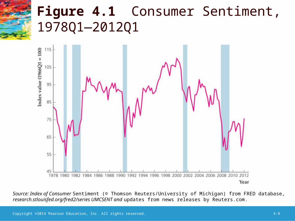
Source: Index of Consumer Sentiment (© Thomson Reuters/University of Michigan) from FRED database, research.stlouisfed.org/fred2/series UMCSENT and updates from news releases by Reuters.com.
Figure 4.1 Consumer Sentiment, 1978Q1—2012Q1
Copyright ©2014 Pearson Education, Inc. All rights reserved. 4-10
Consumption and Saving
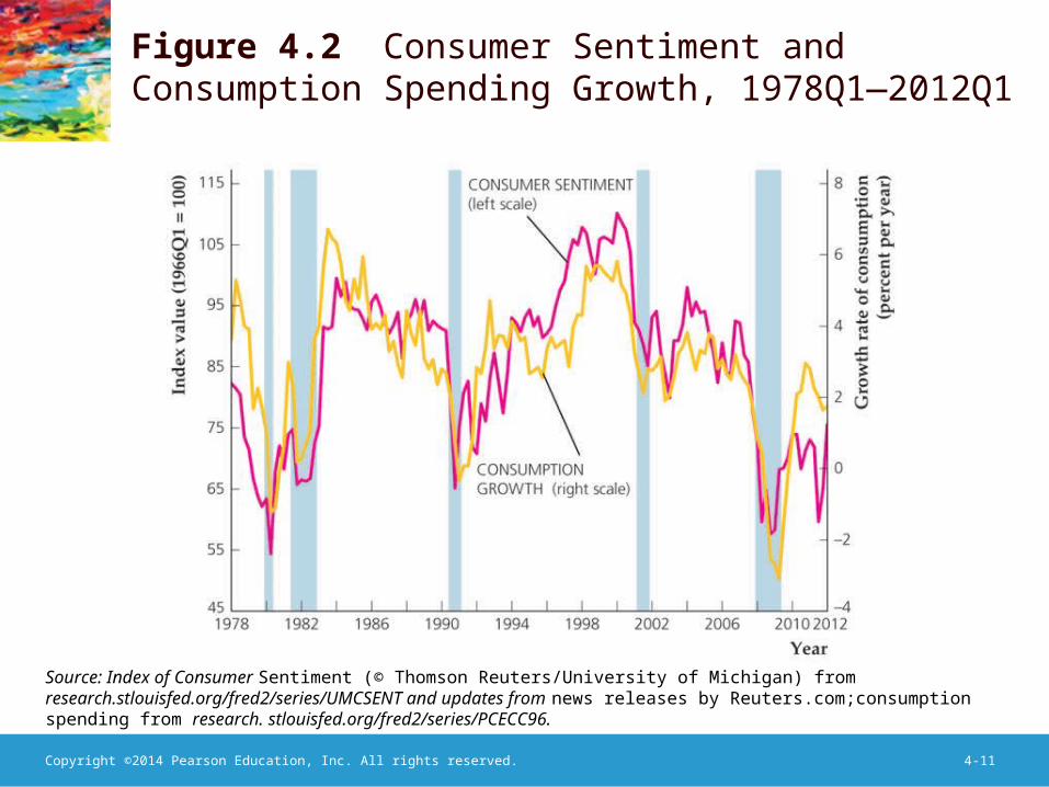
• Application: consumer sentiment and forecasts of consumer spending– Data on consumer spending are correlated with
data on consumer confidence (Fig. 4.2)
Copyright ©2014 Pearson Education, Inc. All rights reserved. 4-11
Source: Index of Consumer Sentiment (© Thomson Reuters/University of Michigan) from research.stlouisfed.org/fred2/series/UMCSENT and updates from news releases by Reuters.com;consumption spending from research. stlouisfed.org/fred2/series/PCECC96.
Figure 4.2 Consumer Sentiment and Consumption Spending Growth, 1978Q1—2012Q1
Copyright ©2014 Pearson Education, Inc. All rights reserved. 4-12
Consumption and Saving
• Application: consumer sentiment and forecasts of consumer spending– Data on consumer spending are correlated with
data on consumer confidence (Fig. 4.2)– But formal statistical analysis shows that data on
consumer confidence do not improve forecasts of consumer spending based on real-time data
Copyright ©2014 Pearson Education, Inc. All rights reserved. 4-13
Consumption and Saving
• Effect of changes in wealth– Increase in wealth raises current consumption,
so lowers current saving
Copyright ©2014 Pearson Education, Inc. All rights reserved. 4-14
Consumption and Saving
• Effect of changes in real interest rate– Increased real interest rate has two opposing
effects• Substitution effect: Positive effect on saving, since rate
of return is higher; greater reward for saving elicits more saving
• Income effect– For a saver: Negative effect on saving, since it takes less
saving to obtain a given amount in the future (target saving)
– For a borrower: Positive effect on saving, since the higher real interest rate means a loss of wealth
• Empirical studies have mixed results; probably a slight increase in aggregate saving
Copyright ©2014 Pearson Education, Inc. All rights reserved. 4-15
Consumption and Saving
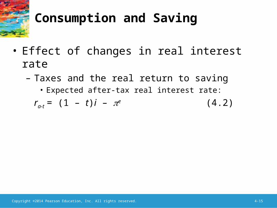
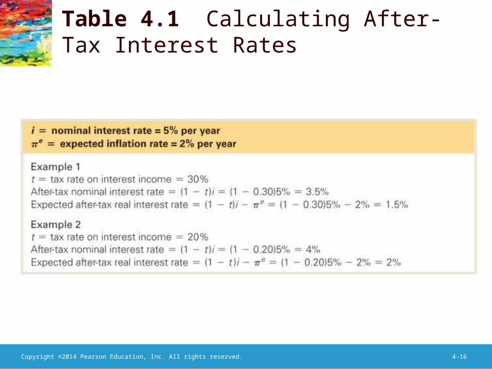
• Effect of changes in real interest rate– Taxes and the real return to saving
• Expected after-tax real interest rate:
ra-t = (1 – t)i – e (4.2)
Copyright ©2014 Pearson Education, Inc. All rights reserved. 4-16
Table 4.1 Calculating After-Tax Interest Rates
Copyright ©2014 Pearson Education, Inc. All rights reserved. 4-17
Consumption and Saving
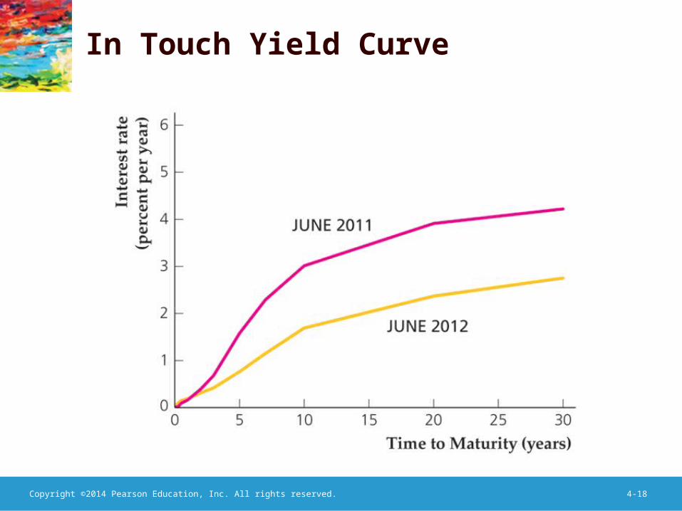
• In touch with data and research: interest rates– Discusses different interest rates, default risk,
term structure (yield curve), and tax status– Since interest rates often move together, we
frequently refer to “the” interest rate – Yield curve: relationship between life of a bond
and the interest rate it pays
Copyright ©2014 Pearson Education, Inc. All rights reserved. 4-18
In Touch Yield Curve
Copyright ©2014 Pearson Education, Inc. All rights reserved. 4-19
Consumption and Saving
• Fiscal policy– Affects desired consumption through changes in
current and expected future income– Directly affects desired national saving,
Sd = Y – Cd – G
Copyright ©2014 Pearson Education, Inc. All rights reserved. 4-20
Consumption and Saving
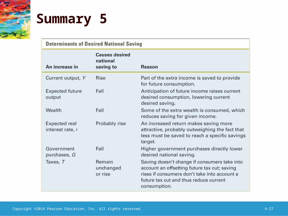
• Fiscal policy– Government purchases (temporary increase)
• Higher G financed by higher current taxes reduces after-tax income, lowering desired consumption
• Even true if financed by higher future taxes, if people realize how future incomes are affected
• Since Cd declines less than G rises, national saving (Sd = Y – Cd – G) declines
• So government purchases reduce both desired consumption and desired national saving
Copyright ©2014 Pearson Education, Inc. All rights reserved. 4-21
Consumption and Saving
• Fiscal policy– Taxes
• Lump-sum tax cut today, financed by higher future taxes
• Decline in future income may offset increase in current income; desired consumption could rise or fall
Copyright ©2014 Pearson Education, Inc. All rights reserved. 4-22
Consumption and Saving
• Fiscal policy– Taxes
• Ricardian equivalence proposition– If future income loss exactly offsets current income gain,
no change in consumption– Tax change affects only the timing of taxes, not their
ultimate amount (present value)– In practice, people may not see that future taxes will rise
if taxes are cut today; then a tax cut leads to increased desired consumption and reduced desired national saving
Copyright ©2014 Pearson Education, Inc. All rights reserved. 4-23
Consumption and Saving
• Application: How consumers respond to tax rebates– The government provided tax rebates in recessions of
2001 and 2007-2009, hoping to stimulate the economy– Research by Shapiro and Slemrod suggests that
consumers did not increase spending much in 2001, when the government provided a similar tax rebate
– New research by Agarwal, Liu, and Souleles finds that even though consumers originally saved much of the tax rebate, later they increased spending and increased their credit-card debt
Copyright ©2014 Pearson Education, Inc. All rights reserved. 4-24
Consumption and Saving
• Application: How consumers respond to tax rebates– The new research comes from credit-card
payments, purchases, and debt over time– People getting the tax rebates initially made
additional payments on their credit cards, paying down their balances; but after nine months they had increased their purchases and had more credit-card debt than before the tax rebate
Copyright ©2014 Pearson Education, Inc. All rights reserved. 4-25
Consumption and Saving
• Application: How consumers respond to tax rebates– Younger people, who were more likely to face
binding borrowing constraints, increased their purchases on credit cards the most of any group in response to the tax rebate
– People with high credit limits also tended to pay off more of their balances and spent less, as they were less likely to face binding borrowing constraints and behaved more in the manner suggested by Ricardian equivalence
Copyright ©2014 Pearson Education, Inc. All rights reserved. 4-26
Consumption and Saving
• Application: How consumers respond to tax rebates– New evidence on the tax rebates in 2008 and
2009 was provided in a research paper by Parker et al.
• Consumers spent 50%-90% of the tax rebates• Inconsistent with Ricardian equivalence
Copyright ©2014 Pearson Education, Inc. All rights reserved. 4-27
Summary 5
Copyright ©2014 Pearson Education, Inc. All rights reserved. 4-28
Investment
• Why is investment important?– Investment fluctuates sharply over the business
cycle, so we need to understand investment to understand the business cycle
– Investment plays a crucial role in economic growth
Copyright ©2014 Pearson Education, Inc. All rights reserved. 4-29
Investment
• The desired capital stock– Desired capital stock is the amount of capital
that allows firms to earn the largest expected profit
– Desired capital stock depends on costs and benefits of additional capital
– Since investment becomes capital stock with a lag, the benefit of investment is the future marginal product of capital (MPKf)
Copyright ©2014 Pearson Education, Inc. All rights reserved. 4-30
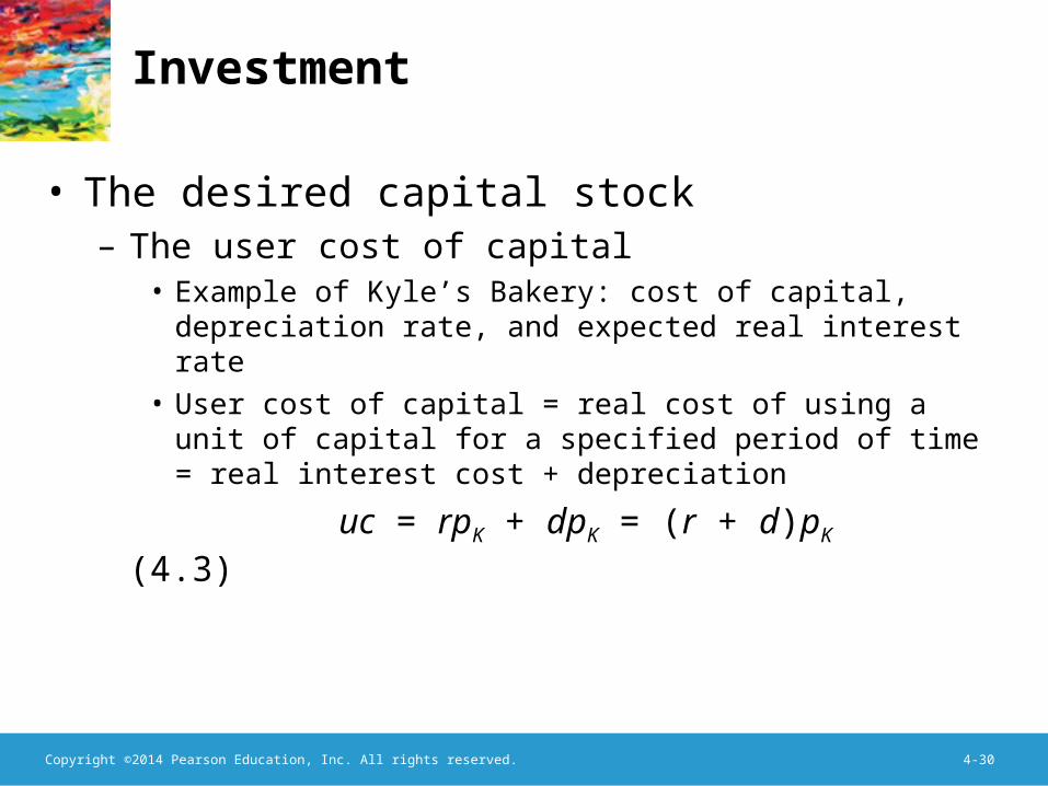
Investment
• The desired capital stock– The user cost of capital
• Example of Kyle’s Bakery: cost of capital, depreciation rate, and expected real interest rate
• User cost of capital = real cost of using a unit of capital for a specified period of time = real interest cost + depreciation
uc = rpK + dpK = (r + d)pK (4.3)
Copyright ©2014 Pearson Education, Inc. All rights reserved. 4-31
Investment
• The desired capital stock– Determining the desired capital stock (Fig. 4.3)
Copyright ©2014 Pearson Education, Inc. All rights reserved. 4-32
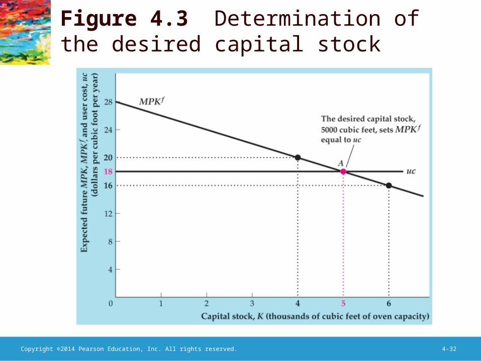
Figure 4.3 Determination of the desired capital stock
Copyright ©2014 Pearson Education, Inc. All rights reserved. 4-33
Investment
• The desired capital stock– Desired capital stock is the level of capital stock
at which MPKf = uc– MPKf falls as K rises due to diminishing marginal
productivity– uc doesn’t vary with K, so is a horizontal line
Copyright ©2014 Pearson Education, Inc. All rights reserved. 4-34
Investment
• The desired capital stock– If MPKf > uc, profits rise as K is added (marginal
benefits > marginal costs)– If MPKf uc, profits rise as K is reduced
(marginal benefits < marginal costs)– Profits are maximized where MPKf = uc
Copyright ©2014 Pearson Education, Inc. All rights reserved. 4-35
Investment
• Changes in the desired capital stock– Factors that shift the MPKf curve or change the
user cost of capital cause the desired capital stock to change
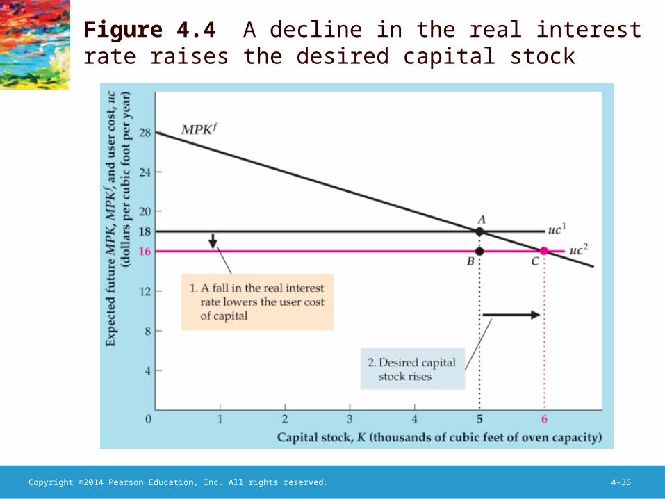
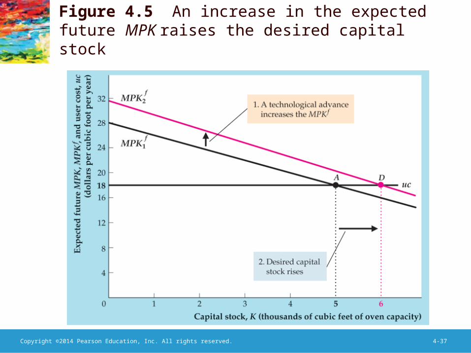
– These factors are changes in the real interest rate, depreciation rate, price of capital, or technological changes that affect the MPKf (Fig. 4.4 shows effect of change in uc; Fig. 4.5 shows effect of change in MPKf)
Copyright ©2014 Pearson Education, Inc. All rights reserved. 4-36
Figure 4.4 A decline in the real interest rate raises the desired capital stock
Copyright ©2014 Pearson Education, Inc. All rights reserved. 4-37
Figure 4.5 An increase in the expected future MPK raises the desired capital stock
Copyright ©2014 Pearson Education, Inc. All rights reserved. 4-38
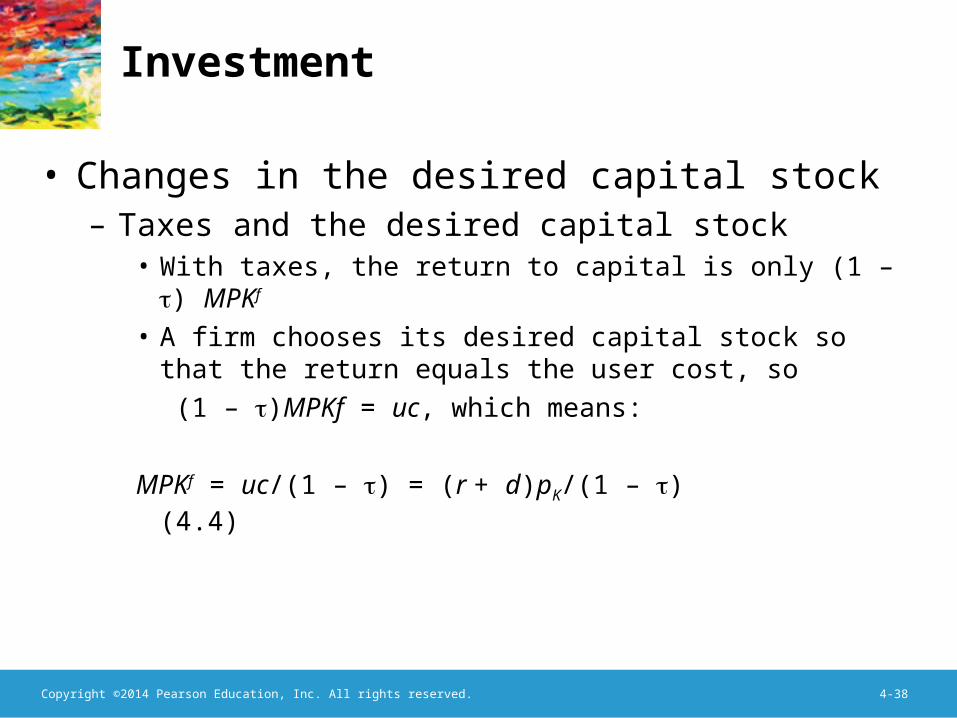
Investment
• Changes in the desired capital stock– Taxes and the desired capital stock
• With taxes, the return to capital is only (1 – ) MPKf
• A firm chooses its desired capital stock so that the return equals the user cost, so (1 – )MPKf = uc, which means:
MPKf = uc/(1 – ) = (r + d)pK/(1 – ) (4.4)
Copyright ©2014 Pearson Education, Inc. All rights reserved. 4-39
Investment
• Changes in the desired capital stock– Taxes and the desired capital stock
• Tax-adjusted user cost of capital is uc/(1 – )• An increase in τ raises the tax-adjusted user cost and
reduces the desired capital stock
Copyright ©2014 Pearson Education, Inc. All rights reserved. 4-40
Investment
• Changes in the desired capital stock– Taxes and the desired capital stock
• In reality, there are complications to the tax-adjusted user cost
– We assumed that firm revenues were taxed» In reality, profits, not revenues, are taxed» So depreciation allowances reduce the tax paid by
firms, because they reduce profits– Investment tax credits reduce taxes when firms make
new investments
Copyright ©2014 Pearson Education, Inc. All rights reserved. 4-41
Investment
• Changes in the desired capital stock– Taxes and the desired capital stock
• In reality, there are complications to the tax-adjusted user cost
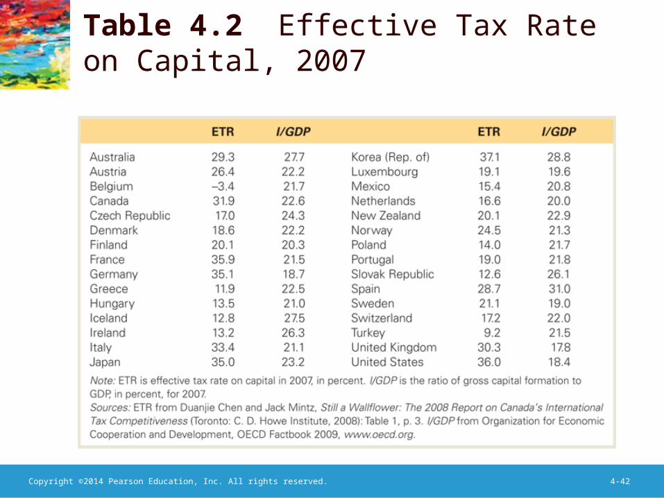
– Summary measure: the effective tax rate—the tax rate on firm revenue that would have the same effect on the desired capital stock as do the actual provisions of the tax code
– Table 4.2 shows effective tax rates for many different countries
Copyright ©2014 Pearson Education, Inc. All rights reserved. 4-42
Table 4.2 Effective Tax Rate on Capital, 2007
Copyright ©2014 Pearson Education, Inc. All rights reserved. 4-43
Investment
• Application: measuring the effects of taxes on investment– Do changes in the tax rate have a significant
effect on investment? – A 1994 study by Cummins, Hubbard, and
Hassett found that after major tax reforms, investment responded strongly; elasticity about –0.66 (of investment to user cost of capital)
Copyright ©2014 Pearson Education, Inc. All rights reserved. 4-44
Investment
• From the desired capital stock to investment– The capital stock changes from two opposing
channels• New capital increases the capital stock; this is gross
investment• The capital stock depreciates, which reduces the
capital stock
Copyright ©2014 Pearson Education, Inc. All rights reserved. 4-45
Investment
• From the desired capital stock to investment– Net investment = gross investment (I) minus
depreciation: Kt+1 – Kt = It – dKt (4.5)
where net investment equals the change in the capital stock
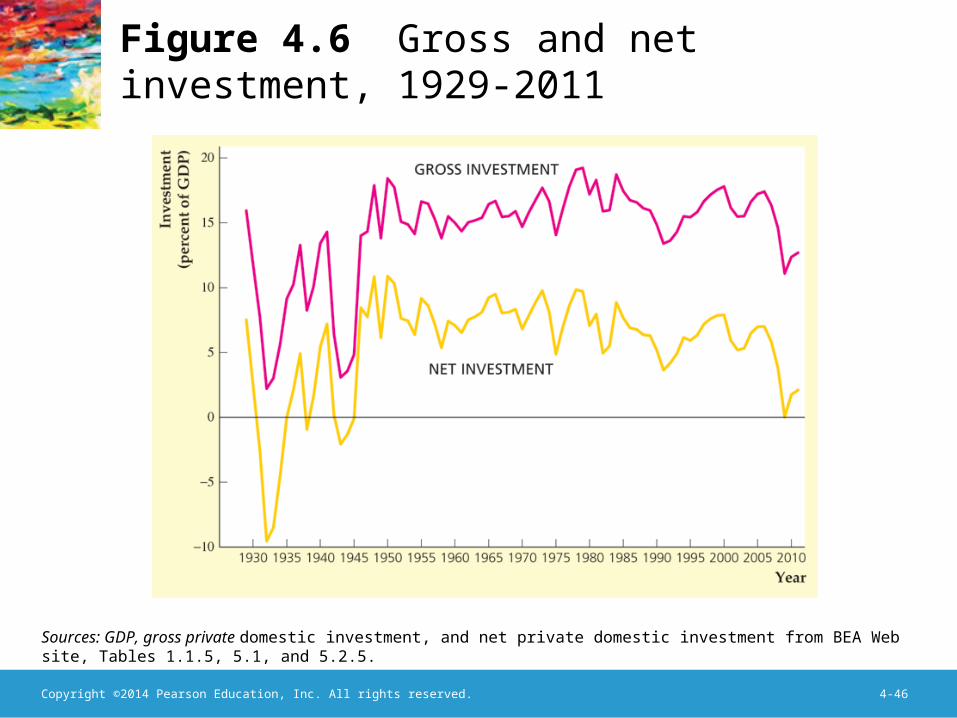
– Fig. 4.6 shows gross and net investment for the United States
Copyright ©2014 Pearson Education, Inc. All rights reserved. 4-46
Figure 4.6 Gross and net investment, 1929-2011
Sources: GDP, gross private domestic investment, and net private domestic investment from BEA Web site, Tables 1.1.5, 5.1, and 5.2.5.
Copyright ©2014 Pearson Education, Inc. All rights reserved. 4-47
Investment
• From the desired capital stock to investment– Rewriting (4.5) gives It = Kt+1 – Kt + dKt
– If firms can change their capital stocks in one period, then the desired capital stock (K*) = Kt+1
– So It = K* – Kt + dKt (4.6)
Copyright ©2014 Pearson Education, Inc. All rights reserved. 4-48
Investment
• From the desired capital stock to investment– Thus investment has two parts
• Desired net increase in the capital stock over the year (K* – Kt)
• Investment needed to replace depreciated capital (dKt)
Copyright ©2014 Pearson Education, Inc. All rights reserved. 4-49
Investment
• From the desired capital stock to investment– Lags and investment
• Some capital can be constructed easily, but other capital may take years to put in place
• So investment needed to reach the desired capital stock may be spread out over several years
Copyright ©2014 Pearson Education, Inc. All rights reserved. 4-50
Investment
• In touch with data and research: investment and the stock market– Firms change investment in the same direction
as the stock market: Tobin’s q theory of investment
– If market value > replacement cost, then firm should invest more
– Tobin’s q = capital’s market value divided by its replacement cost
• If q < 1, don’t invest• If q > 1, invest more
Copyright ©2014 Pearson Education, Inc. All rights reserved. 4-51
Investment
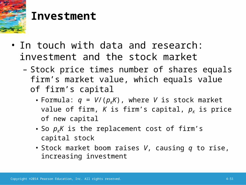
• In touch with data and research: investment and the stock market– Stock price times number of shares equals firm’s
market value, which equals value of firm’s capital
• Formula: q = V/(pKK), where V is stock market value of firm, K is firm’s capital, pK is price of new capital
• So pKK is the replacement cost of firm’s capital stock
• Stock market boom raises V, causing q to rise, increasing investment
Copyright ©2014 Pearson Education, Inc. All rights reserved. 4-52
Investment
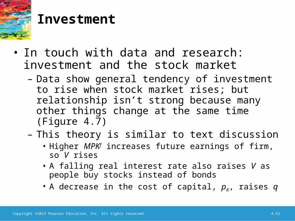
• In touch with data and research: investment and the stock market– Data show general tendency of investment to
rise when stock market rises; but relationship isn’t strong because many other things change at the same time (Figure 4.7)
– This theory is similar to text discussion• Higher MPKf increases future earnings of firm, so V
rises• A falling real interest rate also raises V as people buy
stocks instead of bonds• A decrease in the cost of capital, pK, raises q
Copyright ©2014 Pearson Education, Inc. All rights reserved. 4-53
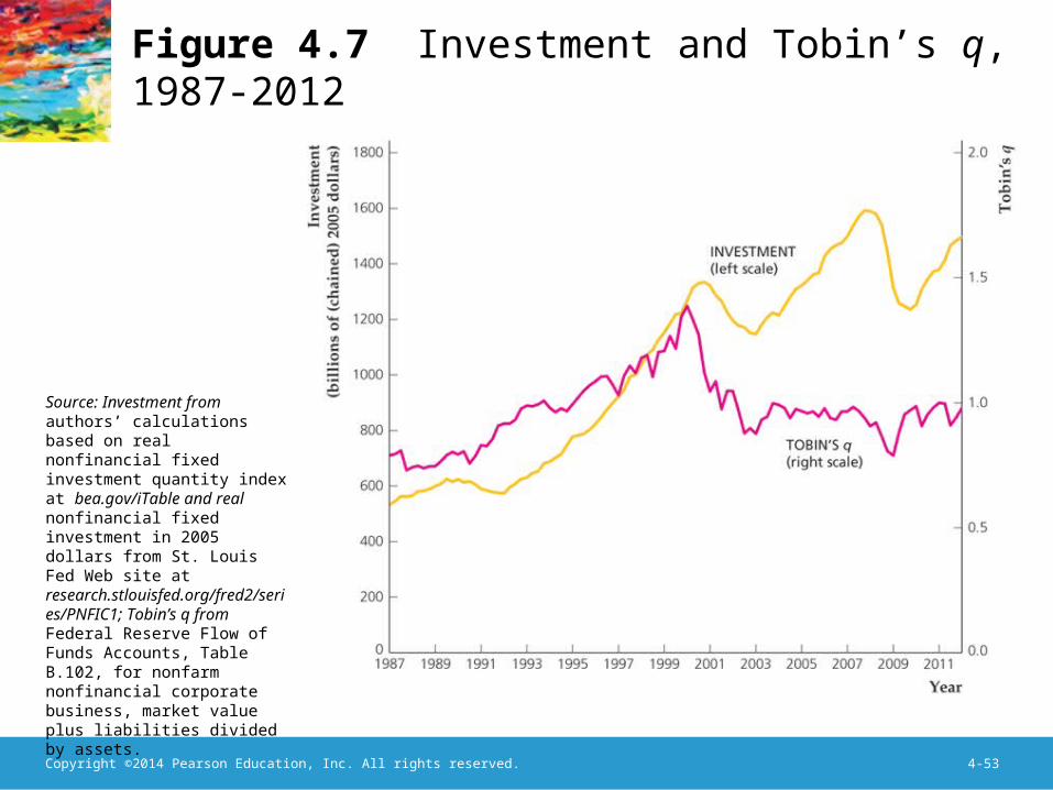
Figure 4.7 Investment and Tobin’s q, 1987-2012
Source: Investment from authors’ calculations based on real nonfinancial fixed investment quantity index at bea.gov/iTable and real nonfinancial fixed investment in 2005 dollars from St. Louis Fed Web site at research.stlouisfed.org/fred2/series/PNFIC1; Tobin’s q from Federal Reserve Flow of Funds Accounts, Table B.102, for nonfarm nonfinancial corporate business, market value plus liabilities divided by assets.

Copyright ©2014 Pearson Education, Inc. All rights reserved. 4-54
Investment
• Investment in inventories and housing– Marginal product of capital and user cost also
apply, as with equipment and structures
Copyright ©2014 Pearson Education, Inc. All rights reserved. 4-55
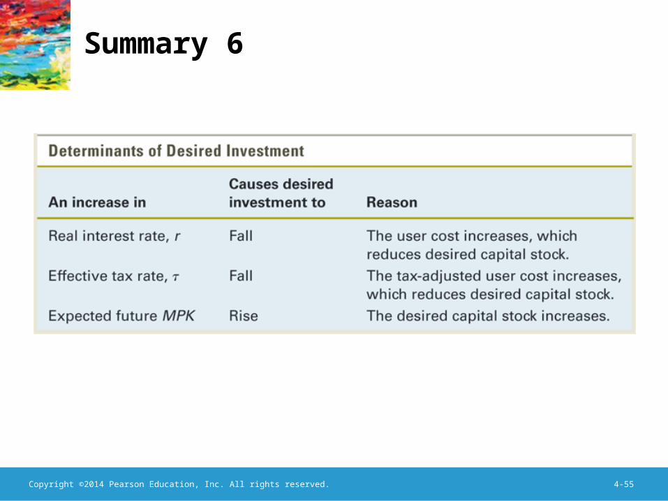
Summary 6
Copyright ©2014 Pearson Education, Inc. All rights reserved. 4-56
Goods Market Equilibrium
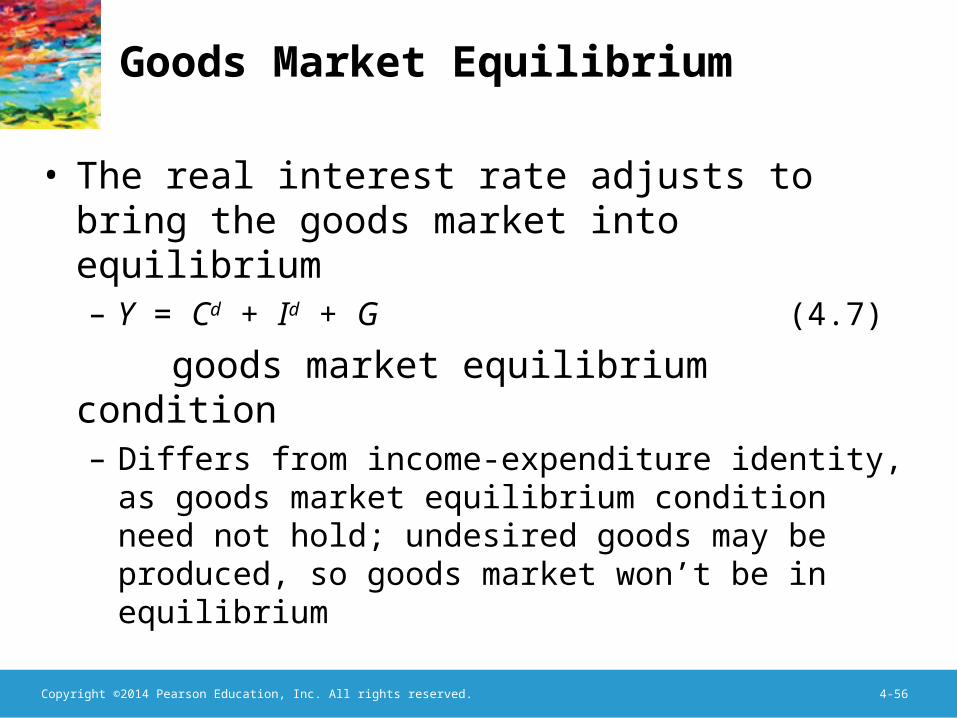
• The real interest rate adjusts to bring the goods market into equilibrium– Y = Cd + Id + G (4.7)
goods market equilibrium condition– Differs from income-expenditure identity, as
goods market equilibrium condition need not hold; undesired goods may be produced, so goods market won’t be in equilibrium
Copyright ©2014 Pearson Education, Inc. All rights reserved. 4-57
Goods Market Equilibrium
• Alternative representation: since• Sd = Y – Cd – G, • Sd = Id (4.8)
Copyright ©2014 Pearson Education, Inc. All rights reserved. 4-58
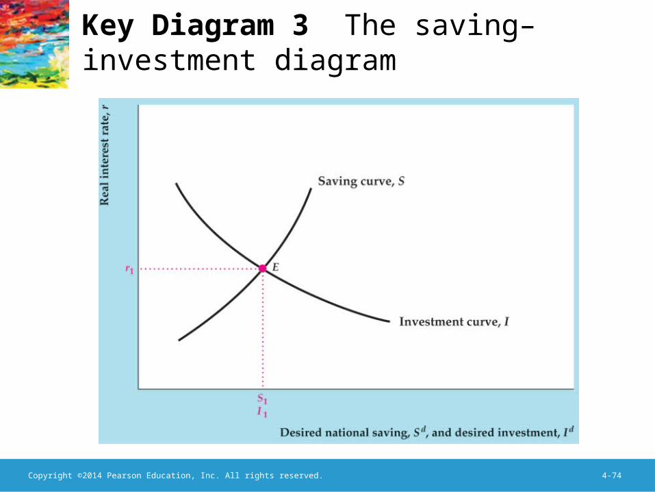
Goods Market Equilibrium
• The saving-investment diagram • Plot Sd vs. Id (Key Diagram 3; text Fig. 4.8)
Copyright ©2014 Pearson Education, Inc. All rights reserved. 4-59
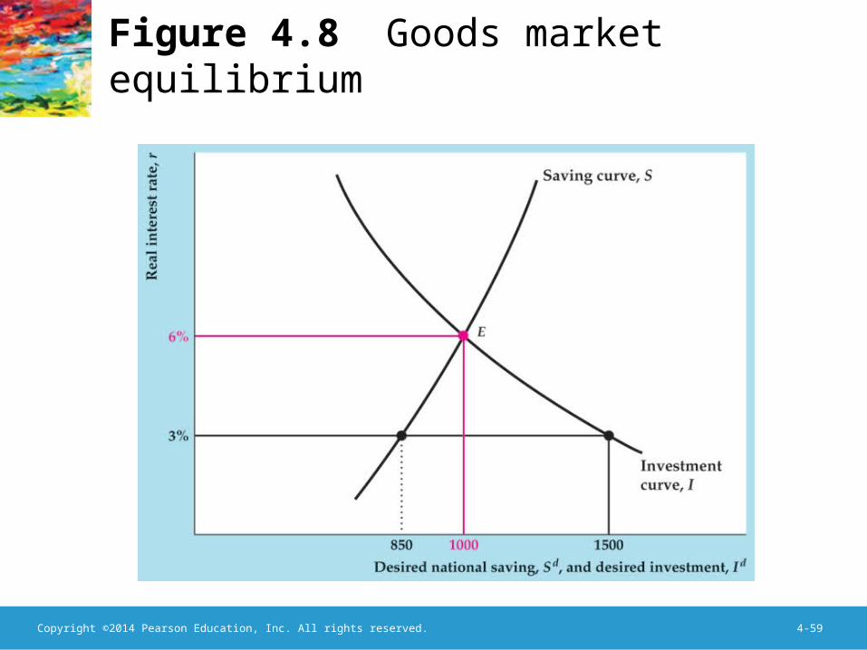
Figure 4.8 Goods market equilibrium
Copyright ©2014 Pearson Education, Inc. All rights reserved. 4-60
Goods Market Equilibrium
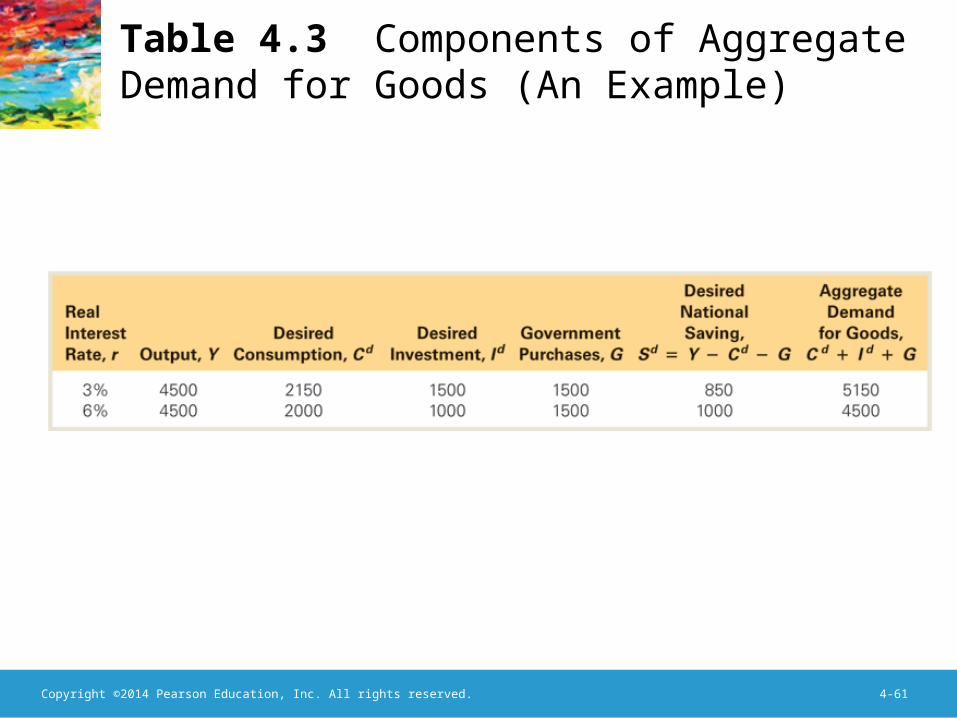
• The saving-investment diagram – Equilibrium where Sd = Id
– How to reach equilibrium? Adjustment of r– See text example (Table 4.3)
Copyright ©2014 Pearson Education, Inc. All rights reserved. 4-61
Table 4.3 Components of Aggregate Demand for Goods (An Example)
Copyright ©2014 Pearson Education, Inc. All rights reserved. 4-62
Goods Market Equilibrium
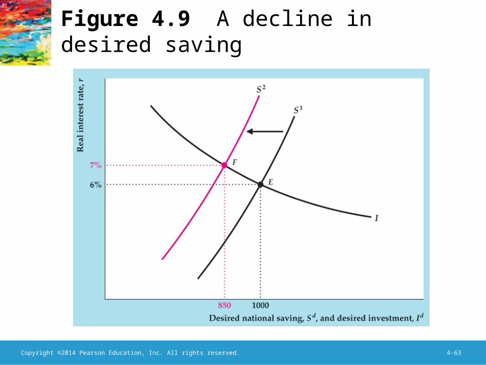
• Shifts of the saving curve– Saving curve shifts right due to a rise in current
output, a fall in expected future output, a fall in wealth, a fall in government purchases, a rise in taxes (unless Ricardian equivalence holds, in which case tax changes have no effect)
– Example: Temporary increase in government purchases shifts S left
– Result of lower savings: higher r, causing crowding out of I (Fig. 4.8)
Copyright ©2014 Pearson Education, Inc. All rights reserved. 4-63
Figure 4.9 A decline in desired saving
Copyright ©2014 Pearson Education, Inc. All rights reserved. 4-64
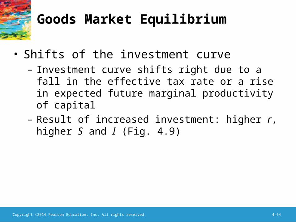
Goods Market Equilibrium
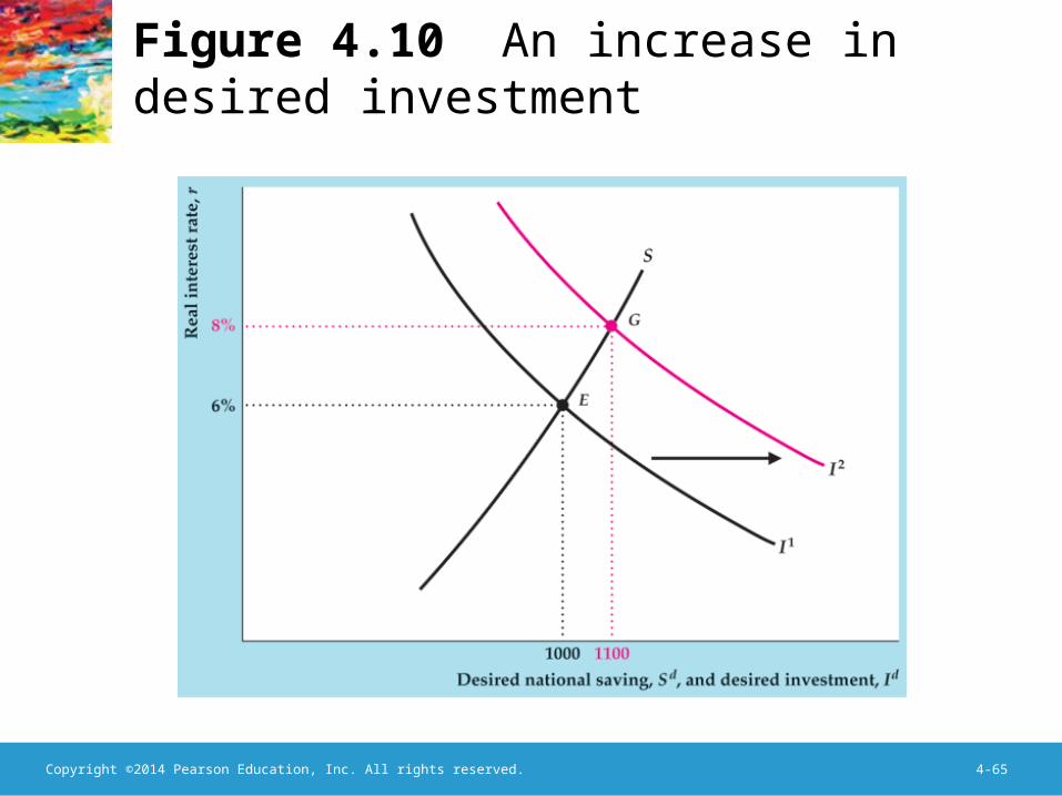
• Shifts of the investment curve– Investment curve shifts right due to a fall in the
effective tax rate or a rise in expected future marginal productivity of capital
– Result of increased investment: higher r, higher S and I (Fig. 4.9)
Copyright ©2014 Pearson Education, Inc. All rights reserved. 4-65
Figure 4.10 An increase in desired investment
Copyright ©2014 Pearson Education, Inc. All rights reserved. 4-66
Goods Market Equilibrium
• Application: Macroeconomic consequences of the boom and bust in stock prices– Sharp changes in stock prices affect
consumption spending (a wealth effect) and capital investment (via Tobin’s q)
– Data in Fig. 4.11
Copyright ©2014 Pearson Education, Inc. All rights reserved. 4-67
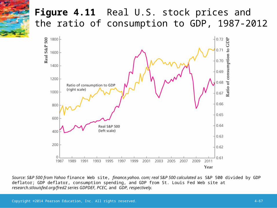
Figure 4.11 Real U.S. stock prices and the ratio of consumption to GDP, 1987-2012
Source: S&P 500 from Yahoo finance Web site, finance.yahoo. com; real S&P 500 calculated as S&P 500 divided by GDP deflator; GDP deflator, consumption spending, and GDP from St. Louis Fed Web site at research.stlouisfed.org/fred2 series GDPDEF, PCEC, and GDP, respectively.
Copyright ©2014 Pearson Education, Inc. All rights reserved. 4-68
Goods Market Equilibrium
• The boom and bust in stock prices– Consumption and the 1987 crash
• When the stock market crashed in 1987, wealth declined by about $1 trillion
• Consumption fell somewhat less than might be expected, and it wasn’t enough to cause a recession
• There was a temporary decline in confidence about the future, but it was quickly reversed
• The small response may have been because there had been a large run-up in stock prices between December 1986 and August 1987, so the crash mostly erased this run-up
Copyright ©2014 Pearson Education, Inc. All rights reserved. 4-69
Goods Market Equilibrium
• The boom and bust in stock prices– Consumption and the rise in stock market wealth
in the 1990s• Stock prices more than tripled in real terms • But consumption was not strongly affected by the
runup in stock prices
Copyright ©2014 Pearson Education, Inc. All rights reserved. 4-70
Goods Market Equilibrium
• The boom and bust in stock prices– Consumption and the decline in stock prices in
the early 2000s• In the early 2000s, wealth in stocks declined by about
$5 trillion• But consumption spending increased as a share of GDP
in that period
Copyright ©2014 Pearson Education, Inc. All rights reserved. 4-71
Goods Market Equilibrium
• The boom and bust in stock prices– Investment and the declines in the stock market
in the 2000s• Investment and Tobin’s q were correlated in 2000 and
2008, when the stock market fell sharply• Investment tended to lag the decline in the stock
market, reflecting lags in the process of making investment decisions
Copyright ©2014 Pearson Education, Inc. All rights reserved. 4-72
Goods Market Equilibrium
• The boom and bust in stock prices– The financial crisis of 2008
• Stock prices plunged in fall 2008 and early 2009, and home prices fell sharply as well, leading to a large decline in household net wealth
• Despite the decline in wealth, the ratio of consumption to GDP did not decline much
Copyright ©2014 Pearson Education, Inc. All rights reserved. 4-73
Goods Market Equilibrium
• The boom and bust in stock prices– Investment and Tobin’s q
• Investment and Tobin’s q were not closely correlated following the 1987 crash in stock prices
• But the relationship has been tighter in the 1990s and early 2000s, as theory suggests (Fig. 4.11)
Copyright ©2014 Pearson Education, Inc. All rights reserved. 4-74
Key Diagram 3 The saving–investment diagram