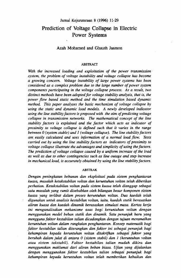
Jurnal Kejuruteraan 8 (1996) 11-29

Prediction of Voltage Collapse in Electric Power Systems

Azah Mohamed and Ghauth Jasmon

ABSTRACT

With the increased loading and exploitation of the power transmISSIOn system. the problem of voltage instability and voltage collapse hos become a growing concern. Voltage instability of large power systems hos been considered as a complex problem due to the large number of power system components participating in the voltage collapse process. As a result, two distinct methods have been adopted for voltage stability anolysis. thot is. the power flow based static method and the time simulation based dynamic method. This paper analyses the basic mechonism of voltage col/apse by using the static and dynomic load models. A newly developed indicator using the line stability factors is proposed with the aim of predicting voltage collapse in transmission networks. The mathematical concept of the line stability factors is explained and the factor which acts as indicator of proximity to voltage col/apse is defined such that it varies in the range between 0 (system stable) and J (voltage col/apse). The line stability factors are. easily calculated and uses information of a normal load flow. Tests carried out by using the line stability factors as indicators of proximity to voltage col/apse illustrate the advantages and simplicity of using the factors. The prediction of voltage col/apse caused by a uniform increase of the load as well as due to other contingencies such as line outage and step increase in mechanical/oad. is accurately obtained by using the line stability factors.

ABSTRAK

Dengan peningkatan bebanan dan eksploitasi pada sistem penghontaran kuasa. masalah ketakstabilan voltan dan keruntuhan voltan telah diberikan perhatian. Ketakstabilan voltan pada sistem kuasa telah dianggap sebagai satu masalah yang rumit disebabkan oleh bilangan besar kamponen sistem kuasa yang terlwat dalam proses keruntuhon voltan. Dua kaedah telah digunakan untuk analisis kestabilan voltan, iaitu, kaedah statik berasaskan aliran kuasa dan kaedah dinomik berasaskan simulasi masa. Kertas kerja in; menganalisakan mekanisme asas bag; keruntuhan voltan dengan menggunokan model beban statik dan dinamik. Satu penunjuk baru yang mengguno faktor kestabilan talian dicadangkan dengan tujuan meramalkan keruntuhan voltan dalam rangkaian penghontaran. Konsep matematik bagi faktor kestabilan talian diterangkan dan faktor ini sebagai penunjuk bagi kehampiran kepada keruntuhan voltan ditakrifkan sebagai faktor yang berubah dalam julat di antara 0 (sistem stabil) dan J (keruntuhan voltan atau sistem takstabil). Faktor kestabilan talian mudah dikira dan menggunakan maklumat dari aliran beban biasa. Ujian yang dijalankan dengan menggunokan faktor kestabilan talian sebagai penunjuk bag; kehampiran kepada keruntuhon voltan telah memberikan kebaikan dan

12

mudahnya penggunaan faktor itu. Ramalan keruntuhan voltan yang disebabkan oleh peningkatan beban, putusan tatian dan juga pertambahan beban mekanik, lelah diperolehi dengan menggunakan faklor. keslabilan latian.

INTRODUCfION

Several recent power system blackouts were related to voltage collapse, which is characterised by a slow decline in voltage magnitude at load buses which may fmally spread out in the network causing a final rapid decline in voltage magnitude. Voltage collapse is generally dttributed to a lack of reactive power support, increased loading of transmission lines and increase in load demands. As power systems are operating during period of high demand and under stressed conditions, the voltage stability margins are severely reduced. Consequently the study of voltage stability and voltage collapse become a major concern for the secure operation of power systems.

Most of the literature on voltage stability studies have presented methods that are categorised as either static or dynamic methods (Mercede et al. 1988; Chow et aI. 1990; Srivastava et al. 1993; IEEE Service Center 1990). The static method implies that a 'steady-static power flow model has been used, while, the dynamic method implies the use of a model characterised by non-linear differential equations. The majority of research on voltage stability has previously been concentrated on the static aspects (Jiranuchit & Thomas 1988; Lof et aI. 1991; Kessel & F1avitsh 1986; Jamura et aI. 1983; Dc Marco & Overbye 1989; Overbye & Dc Marco 1991) in which a number of performance indices intended to measure the severity of the voltage collapse problem have been proposed. Among them, the minimum singular value in Tiranuchit & Thomas (1988) and Lof et al. (1991) and the voltage stability index based on the load flow feasibility in Kessel & Clavilsh (1986) provide some quantitative measure of proximity to voltage collapse. The performance index proposed in Tamura et aI. (1983) is based on the angular distance between the current stable equilibrium point and the closest unstable equilibrium point in a Euclidean sense. The performance index proposed in De Marco & Overbye (1989) and Overbye & De Marco (1991) measures the energy distance between the current stable equilibrium point and the closest unstable eqUilibrium point using an energy function.

The need tu study and analyse the dynamic aspects of voltage stability has become important because of the influence of the dynamic characteristics of loads, generator field excitation system and the tap changing transformer on voltage stability. Sekine & Ohtsuki (1990) used induction motor model as a dynamic load model to study the dynamic phenomena of voltage collapse. Medani et aI. (1987) established that instability of tap changer dynamics can lead to voltage collapse. Begoric & Phadke (1990) model the system dynamics as the swing dynamic of the generators to illustrate the dynamic simulation of voltage collapse.

This paper presents the phenomena of voltage collapse in a power system by considering both the static and the dynamic aspects. A new voltage collapse, indicatur using the line stability factors is also presented,

13

with the aim of predicting proximity to static and dynamic voltage collapse in interconnected power systems. The line stability factors has been tested on standard test-systems and these factors have shown the distinct advantage of reduced computation and of using normal load flow information.

POWER SYSTEM MODEL

The static load model and the dynamic models for generators, loads and tap­changing transformers are used in this analysis.

MODEL OF INTERCONNECTED POWER SYSTEM

A power system network consisting of generators and loads connected by transmission lines and transformers are considered. The network. is represeDled by power flow network equations, which are expressed in terms of node voltages and admittance as follows:

N N Pk + {L(Gkjej - Bkjij)ek + L(Gkjij + Bkjej)Al = 0

j=1 j=1 (1)

N N Ch + {L(Gkjej - Bkjij)A - .L(Gkjij + ~jej)ekl = 0

)=1 )=1 (2)

STATIC LOAD MODEL

The static load model considered in the analysis is the composite load model which is a combination of constant power, constant current and constant impedance loads. The load real and reactive powers are expressed as function of voltage as follows:

P = p. + P,V + Py'

Q = Q. + Q,V + Q,V'

where,

PI' Q • ... P,V, Q,V .. . P,V', Q. V' .. .

constant power loads constant current loads

constant impedance loads

DYNAMIC MODELS

(3)

(4)

The important devices considered in the dynamic voltage stability analysis are the induction motor loads, the transformer tap changer and the generator field excitation system.

Indnction Motor Load Model The induction motor model adopted is similar to the model used in Sekine & Ohtsuki (1990) in which its equivalent circuit is shown in Figure 1.

14

rmfs

lim

FIGURE I. Equivalent circuit of the induction motor

The electrical input pnwers (i.e. active and reactive powers) to the induction motor are given by these equations:

p. rmls

(e2 + /2) = (rmls)2 + xm2 (5)

Q. xm

(02 + /2) = (rmls)2 + xm2 (6)

where rm, xm resistance and reactance of the equivalent circuit of the induction motor.

s slip of induction motor

The relationship between the electric pnwer injected into the motor and the mechanical load is given by the following equation:

(7)

The dynamic equation of the induction motor is a differential equation described as a function of slip as follows:

ds = ._1_( Pm _ P) dt «l>m' l-s '

where «l>: moment of inertia of induction motor m = 2m, f: frequency of the pnwer system

(8)

Transformer Tap-Cbanger Dynamics The dynamics of the transformer with a transformer tap ratio of l:n is modeled by,

dn

dt = ..!.. (Y. - V') T 0

• (9)

where T, is a IiJiIe cOnstant, V. is the reference voltage and V' is the load voltage.

15

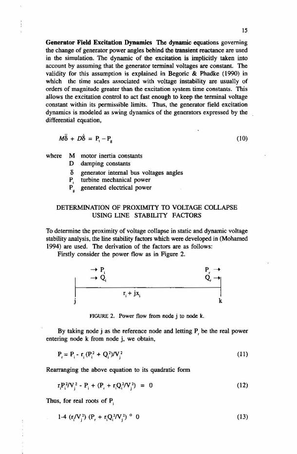
Generator Field Excitation Dynamics The dynamic equations governing the change of generator power angles behind the transient reactance are used in the simulation. The dynamic of the excitation is implicitly taken into account by assuming that the generator terminal voltages are constant. The validity for this assumption is explained in Begoric & Phadke (1990) in which the time scales associated with voltage instability are usually of orders of magnitude greater than the excitation system time constants . This allows the excitation control to act fast enougb to keep the terminal voltage constant within its permissible limits. Thus, the generator field excitation dynamics is modeled as swing dynamics of the generators expressed by the differential equation,

Mii + D~ = P, - P, (10)

where M motor inettia constants D damping constants

B generator internal bus voltages angles P, turbine mechanical power P generated electrical power •

DETERMINATION OF PROXIMITY TO VOLTAGE COLLAPSE USING LINE STABILITY FACTORS

To determine the proximity of voltage collapse in static and dynamic voltage stability analysis, the line stability factors which were developed in (Mohamed 1994) are used. The derivation of the factors are as follows:

Firstl y consider the power flow as in Figure 2.

j k

FIGURE 2. Power flow from node j to node k.

By taking node j as the reference node and letting P, be the real power entering node k from node j, we obtain,

P = P _ r. (P' + (l')N' r I I ( '<i. J

(11)

Rearranging the above equation to its quadratic form

(12)

Thus, for real roots of P;

1-4 (rN.') (P + r.Q.'N .' ) 0 0 I J r I I J

(13)

16

It should be noted that voltage collapse will have already occurred if this condition is not satisfied. By considering the reactive power flow in the same manner as the real power flow, we can derive the reactive power flow condition as:

(14)

By considering the power flow from node k to node j, similarly we can obtain for real roots of P ,.

1-4(r/y,') (-Pi+ri Q,'N,') ~ 0 (15)

and for real roots of Qr ,

1-4(x/y,') (-Qi + Xi P,'N,') ~ 0 (16)

From the above conditions, we obtain four stability limits henceforth called the line stability factors designated as follows:

LPP = 4 (r/y;') (P, + ri Q.'N;') (17)

LQP = 4 (x/y;') (Q, + Xi Pi'N;') (18)

LPN = 4 (r/y,') (-Pi + r, Q,'N,') (19)

LQN = 4 (xiN,') (-Qi + xiP,'N,') (20)

The above four important line stability factors are calculated for all the lines in the system and the line with the highest stability factor value (Le. value closest to 1.0) indicate the proximity to voltage collapse. Thus, the line stability factor can be used as an indicator of proximity to voltage collapse.

SIMULATION OF PROXIMITY TO VOLTAGE COLLAPSE

Both static and dynamic simulations are carried out in the analysis. Proximity to voltage collapse is determined by using load increase or power system state change due a disturbance such as line outage.

STATIC SIMULATION OF VOLTAGE COLLAPSE

In the static simulation, several load flow solutions are obtained by increasing the constant P-Q loads until load flow diverges. At this point, the system is said to collapse with loads of maximum power. The load flow solution very close to the point of voltage collapse is then obtained. The proximity to voltage collapse from a system-wide perspective is determined by using the line stability factors.

17

DYNAMIC SIMULATION OF VOLTAGE COLLAPSE

To detennine the proximity to voltage collapse using time domain simulations, the following approach is used.

1. Solve the base case load flow for a given load level using constant p. Q and induction motor loads.

2. Simulate a disturbance which can be due to a step increase in constant P-Q load or mechanical load, line outage and switching out of shunt capacitors. Consider a disturbance that can simulate the proximity to voltage collapse.

3. Solve the differential equations of the induction motor, tap-changing transformer and the generator field excitation system, at time t, using the Runge-KUlla method.

4. Calculate the system condition at time t by solving the load flow equations.

5. Calculate the active and reactive powers injected to the induction motor, the transformer tap ratio and the generator internal bus angle.

6. Increment the time, t = t + At and repeat the procedure i.e. go to step (3).

TEST RESULTS AND DISCUSSION

The test results of the static and dynamic voltage stability analyses are shown to illustrate the static and dynamic voltage collapse phenomena and the use of line stability factors as indicators of promixity to voltage collapse.

TEST SYSTEMS DESCRIPTION

Two test systems are considered. The first is the 24-bus power system model shown in Figure 3. The system consists of eleven generator buses and thirteen load buses in which the line and bus data for generation and load of the system are given in Appendix A. The second system is the 4-bus power system shown in Figure 4, in which the system is similar to the system used in Sekine & Ohtsuki (1990). The bus, line and machine data of the system are given in Appendix B in which all the per unit values have been referred to 100 MVA base. The 24-bus system is used in the static voltage stability analysis whereas the 4-bus system is used in the dynamic analysis.

STATIC ANALYSIS

In the static simulation of voltage collapse, several load flow solutions are obtained by increasing the constant P-Q loads until load flow diverges. At this point, the system collapses with maximum power of constant P~Q loads. The load flow solution very close to the point of voltage collapse from a system - wide perspective is determined by using the line stability factors.

For the static simulation of voltage collapse in the 24-bus system, the constant P-Q load at bus 14 has been increased to the point of proximity to voltage collapse i.e. when the load at bus 14 becomes (4.1 + 3.1) per unit MVA.

,

••

..

1IUV

FIGURE 3. One-line diagram of 24-bus power system

Bus Bus 2

jO.033 T

'l." JO.O~

1M: Induclion molor FIGURE 4. One-line diagram of 4~bus power system

19

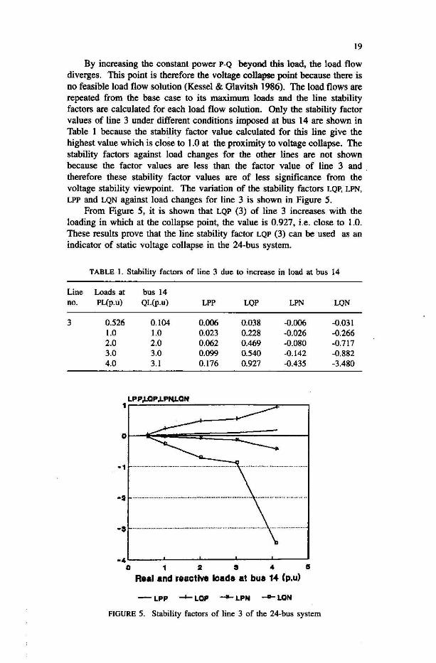
By increasing the constant power P-Q beyond this load, the load flow diverges. This point is therefore the voltage collapse point because there is no feasible load flow solution (Kessel & Glavitsh 1986). The load flows are repeated from the base case to its maximum loads and the line stability factors are calculated for each load flow solution. Only the stability factor values of line 3 under different conditions imposed at bus 14 are shown in Table I because the stability factor value calculated for this line give the highest value whicb is cloSe to 1.0 at the proximity to voltage collapse. The stability factors against load changes for the other lines are not sbown because the factor values are less than the factor value of line 3 and . therefore these stability factor values are of less significance from the voltage stability viewpoint. The variation of the stability factors LQP, LPN. LPP and LQN against load cbanges for line 3 is shown in Figure 5.

From Figure 5, it is shown that LQP (3) of line 3 increases with the loading in which at the collapse point, the value is 0.927, i.e. close to 1.0. These results prove that the line stability factor LQP (3) can be used as an indicator of static voltage collapse in the 24-bus system.

TABLE-I. Stability factors of line 3 due to increase in load at bus 14

Line Loads at bus 14 no. PL(p.u) QL(p.u) LPP LQP LPN LQN

3 0.526 0.104 0.006 0.038 -0.006 -0.031 1.0 1.0 0.023 0.228 -0.026 -0.266 2.0 2.0 0.062 0.469 -0.080 -0.717 3.0 3.0 0.099 0.540 -0.142 -0.882 4.0 3.1 0.176 0.927 -0.435 -3.480

1~LP~P~~~P~~~P~~=O=N~ ____________ ~~ __ -,

-1 ........................................................... .

-I ................................................................................................. ..

-, ............. " .. " .. " .......................... " ........................ ..

_4 L _-'-__ "--_-'-__ -'--_-..J o 1 1 , 4 5

Real and re.ctIve load. at bue 1-4- (p,u)

- LPP ....... LOP --- LPN -- LON

FIGURE 5. Stability factors of line 3 of the 24-bus system

20

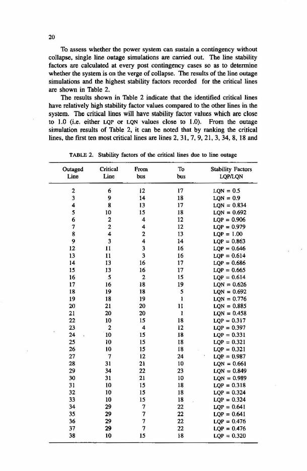
To assess whether the power system can sustain a contingency without collapse, single line outage simulations are carried out. The line stability factors are calculated at every post contingency cases so as to determine whether the system is on the verge of collapse. The results of the line outage simulations and the highest stability factors recorded for the critical lines are shown in Table 2.

The results shown in Table 2 indicate that the identified critical lines have relatively high stability factor values compared to the other lines in the system. The critical lines will have stability factor values which are close to 1.0 (i.e. either LQP or LQN values close to 1.0). From the outage simulation results of Table 2, it can be noted that by ranking the critical lines, the flrst ten most critical lines are lines 2, 31, 7, 9, 21, 3, 34, 8,18 and

TABLE 2. Stability factors of !he critical lines due to line outage

Outaged Critical From To Stability Factors Line Line bus bus LQP/LQN

2 6 12 17 LQN = 0.5 3 9 14 18 LQN = 0.9 4 8 13 17 LQN = 0.834 5 \0 15 18 LQN = 0.692 6 2 4 12 LQP = 0.906 7 2 4 12 LQP = 0.979 8 4 2 13 LQP = 1.00 9 3 4 14 LQP = 0.863

12 II 3 16 LQP = 0.646 13 II 3 16 LQP = 0.614 14 13 16 17 LQP = 0.686 15 13 16 \7 LQP = 0.665 16 5 2 15 LQP = 0.614 17 16 18 19 LQN = 0.626 18 19 18 5 LQN = 0.692 19 18 19 1 LQN = 0.776 20 21 20 II LQN = 0.885 21 20 20 1 LQN = 0.458 22 \0 15 18 LQP = 0.3\7 23 2 4 12 LQP = 0.397 24 \0 15 18 LQP = 0.331 25 \0 15 18 LQP = 0.321 26 \0 15 18 LQP = 0.321 27 7 12 24 LQP = 0.987 28 31 21 \0 LQN = 0.661 29 34 22 23 LQN = 0.849 30 31 21 \0 LQN = 0.989 31 10 15 18 LQP = 0.318 32 10 15 18 LQP = 0.324 33 10 15 18 LQP = 0.324 34 29 7 22 LQP = 0.641 35 29 7 22 LQP = 0.641 36 29 7 22 LQP = 0.476 37 29 7 22 LQP = 0.476 38 10 15 18 LQP = 0.320

21

10. The results prove that voltage collapse can also be caused by line outages and that the collapse originates at the critical lines.

DYNAMIC ANALYSIS

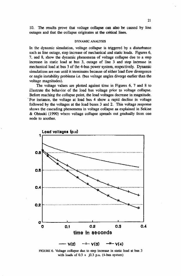
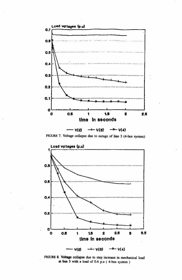
In the dynamic simulation, voltage collapse is triggered by a disturbance such as line outage, step increase of mechanical and static loads. Figures 6, 7, and 8, show the dynamic phenomena of voltage collapse due to a step increase in static load at bus 3, outage of line 3 and step increase in mechanical load at bus 3 of the 4-bus power system, respectively. Dynamic simulations are run until it terminates because of either load flow divergence or angle instability problems i.e. (bus voltage angles diverge earlier than the voltage magnitudes).

The voltage values are plotted against time in Figures 6, 7 and 8 to illustrate the behavior of the load bus voltage prior to voltage collapse. Before reaching the collapse point, the load voltages decrease in magnitude.

'For instance, the voltage at load bus 4 show a rapid decline in voltage followed by the voltages at the load buses 3 and 2. This voltage response shows the cascading phenomena in voltage collapse as explained in Sekine & Ohtsuki (1990) where voltage collapse spreads out gradually from one node to another.

Load voltaQal (p.u) 1r-----~~----------------------.

oL-______ ~ ______ _L ______ ~~ ____ __J

o 0.1 0.2 O.S 0.4 time in seconds

-V(2)

FIGURE 6. Voltage collapse due to step increase in static load at bus 3 with loads of 0.3 + jO.3 p.u. (4-bus system)

0.7 ;L~O._d __ ~~I~~~'~~~'~~ ____________________ --,

0.8 .. .... .. ............. .. .

0.5

0.4 \\ ....... .

0.3t-.. .\.~ ................................................................. .

.... 0.2t-······· ......................................... ... ............. .. ... .. .......................... .

0.1 t-................... . ............................................. .:;;: .................. .. ..... .

oL---~~--~-----L----~ __ --J

o 0.5 1 1.5 1/ 1/.11

time In aeeends

-- V(2) -I- VISl -- V(4)

FIGURE 7. Voltage collapse due to outage of lin. 3 (4-bus system)

1~LO~.=d~VO~II=.~g~ •• ~~~~~) ______________________ ,

..............................

oL-__ ~ __ ~ __ ~ __ ~ __ ~ __ L-~ o 0.5 1 1.S 1/ 2.5 :iI.S

time In aeconds

-- VII) -I- viS) -- V(4)

FIGURE 8. V<!kIge collapse due to step increase in mechanical load at bus 3 with • load of 0.6 p.u ( 4-bus system)

23

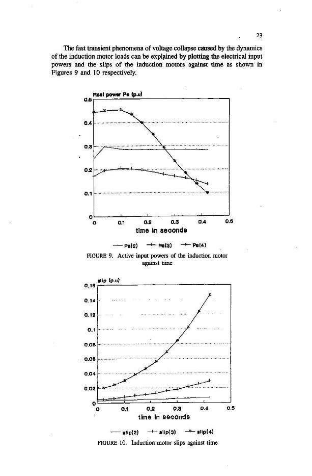
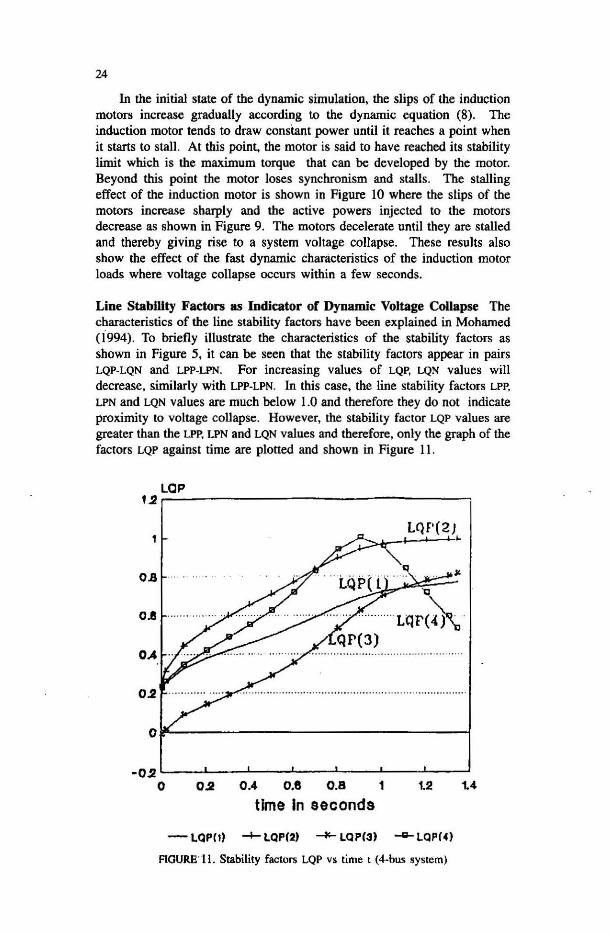
The fast transieni phenomena of voltage collapse cansed by the dynamics of the induction motor loads can be expl,uned by plotting the electrical input powers and the slips of the induction motors against time as shown in Figures 9 and 10 respectively.

Roal _ Pa Ip.u) o~~~~--~~--------------------,

0.4

o.S

0.2

0.1 .................................... .

oL---~----~--~----~--~ o 0.1 0.2 0.3 0.4 0.5

tIme In seconds

- Pa(2) --+- Pe(S) --- Pe(4)

FIGURE 9. Active input powers of the induction motor against time

• _1~;P~~~.u~) __________________________ --, O.lftr· 0.14 .

0.12

0.1

O.OB O.Oft 0.04

O.O:~==:±~~;~~~~===:;:=-__ J o 0.1 0.2 0.3 0.4 O.S

time in aeconds

- .1;P(2) --+- ."p(s) --- '''p(4)

FIGURE 1 O. Induction motor slips against time

24

In the initial state of the dynamic simulation, the slips of the induction motors increase gradually according to the dynamic equation (8). The induction motor tends to draw constant power until it reaches a point when it starts to stall. At this point, the motor is said to have reached its stability limit which is the maximum torque that can be developed by the motor. Beyond this point the motor loses synchronism and stalls. The stalling effect of the induction motor is shown in Figure 10 where the slips of the motors increase sbarply and the active powers injected to the motors decrease as shown in Figure 9. The motors decelerate until they are stalled and thereby giving rise to a system voltage collapse. These results also show the effect of the fast dynamic characteristics of the induction motor loads where voltage collapse occurs within a few seconds.

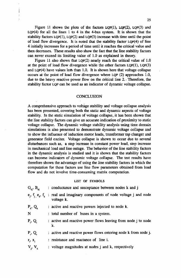
Line StablUty Factors as Indicator of Dynamic Voltage Collapse The characteristics of the line stability factors have been explained in Mohamed (i994). To briefly illustrate the characteristics of the stability factors as shown in Figure 5, it can be seen that the stability factors appear in pairs LQP-LQN and LPP-LPN. For increasing values of LQP, LQN values will decrease, similarly with LPP-LPN. In this case, the line stability factors LPP. LPN and LQN values are much below 1.0 and therefore they do not indicate proximity to voltage collapse. However, the stability factor LQP values are greater than the LPP. LPN and LQN values and therefore, only the graph of the factors LQP against time are plotted and shown in Figure II .

lap 1~r-------------------------------'

lQf'(2) I ' ! ...

0.8 'c

0.8 ············Lqr(~\,· 0.4

O~

O~--------------------------------;

_0~L-__ ~ __ -L __ ~ ____ ~ __ -L __ ~ __ ~

o 0..2 0.4 0.8 0.8 1 12 1.4

time In seconds

-- LQP") -+- LQP(2) -+- LQP(3) ....... LQP(4)

FlGURE·11. Stability factors LQP vs time t (4-bus system)

25

Figure 11 shows the plots of the factors LQP(l), LQp(2), LQP(3) and LQP( 4) for aU the lines I to 4 in the 4-bus system. It is shown that the stability factors LQP(I), LQP(2) and LQP(3) increase with time until the point of load flow divergence. It is noted that the stability factor LQP(4) of line 4 initially increases for a period of time until it reaches the critical value and then decreases. These results also show the fact that the line stability factors can never exceed its limiting value of 1.0 as explained in theory.

Figure 11 also shows that LQP(2) nearly reach the critical value of 1.0 at the point of load flow divergence while the other factors LQP(I). LQP(3) and LQP(4) have values le!lS than 1.0. It is shown here that voltage coUapse occurs at the point of load flow divergence where LQP (2) approaches 1.0, due to the heavy reactive power flow on the critical line 2 .. Therefore, the stability factor LQP can be used as an indicator of dynamic voltage coUapse.

CONCLUSION

A comprehensive approach to voltage stability and voltage coUapse analysis has been presented, covering both the static and dynamic aspects of voltage stability. In the static simulation of voltage collapse, it has been shown that the line stability factors can give an accurate indication of proximity to static voltage collapse. The dynamic voltage stability analysis using time domain simulations is also presented to demonstrate dynamic voltage collapse and to show the influence of induction motor loads, transformer tap changer and generator field exciter. Voltage coUapse is shown to occur due to several disturbances such as, a step increase in constant power load, step increase in mechanical load and line outage. The behavior of the line stability factors in the dynamic analysis is studied and it is shown that the stability factors can become indicators of dynamic voltage collapse. The test results have therefore shown the advantage of using the line stability factors in which the computation for these factors use line flow parameters obtained from load flow and do not involve time-consuming matrix computation.

LIST OF SYMBOLS

G'j' B'j conductance and susceptance between nodes k and j

e, f ek, fk real and imaginary components of node voltage j and node

J J. voltage k.

P" Qk active and reactive powers injected to node k.

N total number of buses in a system.

P;, Q; active and reactive power flows leaving from node j to node k.

Pc' Q, active and reactive power flows entering node k from node j.

ri, Xi resistance and reactance of line i.

Vj, V, voltage magnitudes at nodes j and k, respectively

26

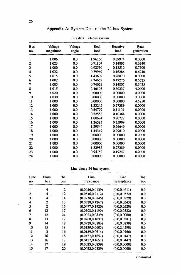
Appendix A: System Data of the 24-bus System

Bus data: 24-bus system

Bus Voltage Voltage Real Reactive Real DO. magnitude angle load load generation

I 1.006 0.0 1.96166 0.39974 0.0000 2 1.023 0.0 0.71804 0.14805 0.6240 3 1.000 0.0 0.92530 0.18510 0.7500 • 4 1.022 0.0 0.79949 0.16286 0.6240 5 1.015 0.0 1.43609 0.28870 0.0000 6 1.002 0.0 2.34659 0.47276 0.6625 7 1.005 0.0 0.74025 0.14805 0.5425 8 1.015 0.0 2.46503 0.50337 4.0000 9 1.020 0.0 0.00000 0.00000 4.0000 10 1.030 0.0 0.00000 0.00000 3.0000 11 1.000 0.0 0.00000 0.00000 4.5850 12 1.000 0.0 l.3~245 0.27389 0.0000 13 1.000 0.0 0.54779 0.11104 0.0000 14 1.000 0.0 0.52558 0.10364 0.0000 IS 1.000 0.0 1.00674 0.20727 0.0000 16 1.000 0.0 1.26583 0.25909 0.0000 17 1.000 0.0 1.29544 0.26649 0.0000 18 1.000 0.0 1.44349 0.29610 0.0000 19 1.000 0.0 0.00000 0.00000 0.0000 20 1.000 0.0 0.00000 0.00000 0.0000 21 1.000 0.0 0.00000 0.00000 0.0000 22 1.000 0.0 1.33985 0.27389 0.0000 23 1.000 0.0 0.94752 0.19247 0.0000 24 1.000 0.0 0.00000 0.00000 0.0000

Line data : 24-bus system

Line From To Line Line Tap no. bus bus impedance susceptance ratio

I 4 2 (0.0026,0.0139) (0.0,0.4611) 0.0 2 4 12 (0.0546,0.2112) (0.0,0.0572) 0.0 3 4 14 (0.0218,0.0845) (0.0,0.0229) 0.0 4 2 13 (0.0328,0.1261) (0.0,0.0343) 0.0 5 2 15 (0.0497,0.1920) (0.0.0.0520) 0.0 6 12 17 (0.0308,0.1190) (0.0,0.0322) 0.0 1 12 24 (0.0023,0.0839) (0.0,0.0000) 0.0 8 13 17 (0.0268,0.1031) (0.0,0.0281 ) 0.0 9 14 18 (0.0228,0.0883) (0.0,0.0239) 0.0 10 15 18 (0.0139,0.0605) (0.0,2.4590) 0.0 11 3 16 (0.0159,0.0614) (0.0,0.0166) 0.0 12 16 18 (0.0427,0.165 I) (0.0,0.0447) 0.0 13 16 17 (0.0427,0.1651) (0.0,0.0447) 0.0 14 11 19 (0.0023,0.0839) (0.0,0.0000) 0.0 15 17 20 (0.0023,0.0839) (0.0,0.0000) 0.0

Continued

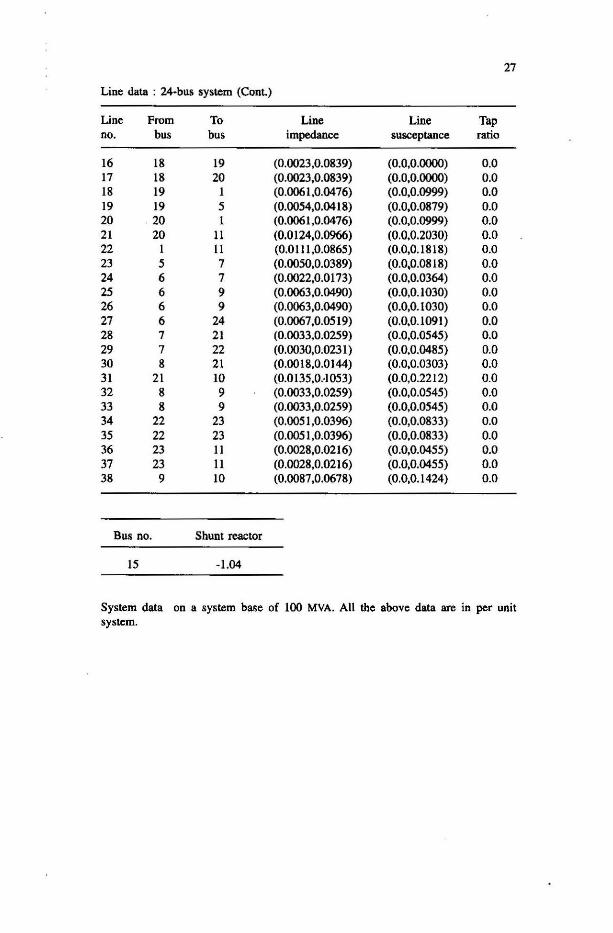
27

Line data: 24·bus system (Cont.)

Line From To Line Line Tap no. bus bus impedance susceptance ratio

16 18 19 (0.0023,0.0839) (0.0,0.0000) 0.0 17 18 20 (0.0023,0.0839) (0.0,0.0000) 0.0 18 19 1 (0.0061,0.0476) (0.0,0.0999) 0.0 19 19 5 (0.0054,0.0418) (0.0,0.0879) 0.0 20 20 1 (0.0061 ,0.0476) (0.0,0.0999) 0.0 21 20 11 (0,0124,0.0966) (0.0,0.2030) 0.0 22 1 11 (0.0111,0.0865) (0.0,0.1818) 0.0 23 5 7 (0.0050,0.0389) (0.0,0.0818) 0.0 24 6 7 (0.0022,0.0173) (0.0,0.0364) 0.0 25 6 9 (0.0063,0.0490) (0.0,0.1030) 0.0 26 6 9 (0.0063,0.0490) (0.0,0.1030) 0.0 27 6 24 (0.0067,0.0519) (0.0,0.1091 ) 0.0 28 7 21 (0.0033,0.0259) (0.0,0.0545) 0.0 29 7 22 (0.0030,0.0231) (0.0,0.0485) 0.0 30 8 21 (0.0018,0.0144) (0.0,0.0303) 0.0 31 21 10 (0.0135,0 .. 1053) (0.0,0.2212) 0.0 32 8 9 (0.0033,0.0259) (0.0,0.0545) 0.0 33 8 9 (0.0033,0.0259) (0.0,0.0545) 0.0 34 22 23 (0.0051 ,0.0396) (0.0,0.0833) 0.0 35 22 23 (0.0051,0.0396) (0.0.0.0833) 0.0 36 23 11 (0.0028,0.0216) (0.0,0.0455) 0.0 37 23 11 (0.0028,0.0216) (0.0,0.0455) 0.0 38 9 10 (0.0087,0.0678) (0.0,0.1424) 0.0

Bus no. Shunt reactor

15 -1.04

System data OD a system base of 100 MVA. All the above data are in per unit system.

28

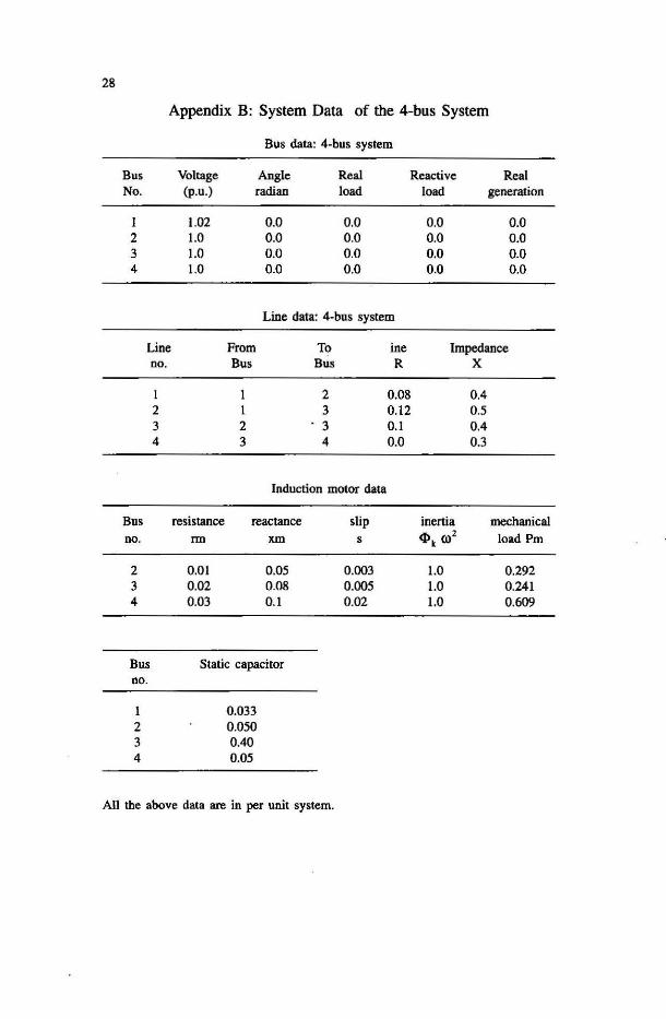
Appendix B: System Data of the 4-bus System

Bus data: 4·bus system

Bus Voltage Angle Real Reactive Real No. (p.u.) radian load load generation

I 1.02 0.0 0.0 0.0 0.0 2 1.0 0.0 0.0 0.0 0.0 3 1.0 0.0 0.0 0.0 0.0 4 1.0 0.0 0.0 0.0 0.0

Line data: 4·bus system

Line From To ine Impedance no. Bus Bus R X

1 2 0.08 0.4 2 I 3 0.12 0.5 3 2 3 0.1 0.4 4 3 4 0.0 0.3

Induction motor data

Bus resistance reactance slip inenia mechanical no. rm xm s cI> ro' , load Pm

2 om 0.05 0.003 1.0 0.292 3 0.02 0.08 0.005 1.0 0.241 4 0.03 0.1 0.02 1.0 0.609

Bus Static capacitor no.

I 0.033 2 0.050 3 0.40 4 0.05

All the above data are in per unit system.

29

REFERENCES

Mercede, F., Chow, J.C., Yon, H. & Fischl, R. 1988. A Fnunework to Predict Vollage Collapse in Power Systems. IEEE Trans. on Power ~ystems 3(4): 1807-1811.

Chow, J.C .. Fishcbl, R & Yan, H. 1990. On the Evaluation of Voltage Collapse Criteria. IEEE Trans. on Power Systems. 5(2): 612 . 619.

Srivastava, K.M., Srivastava, S.C. & Kalra, K. 1993. Voltage Instability in Power System - An Overview and Key Issues. ISEDEM. Third International Symposium on Electrical Distribution and Energy Management. Singapore, 676-683.

IEEE Publications 90th 0358-2-PWRS. 1990. Voltage Stability of Power Systems: Concepts, Analytical Tools & Industry Experience. New Jersey: IEEE Service Centre.

Tiranuchit, A. & Thomas, RJ. 1988. A Posturing Strategy Against .Voltage Instabilities in Electric Power Systems. IEEE Trans. on Power Systems. 3: 87 - 93.

Lof, P.A., Smed, Andersson, T.G. & Hill, D.J. 1991. Fast Calculation of a Voltage Stability Index. IEEFJPES Winter Meeting WM 203-0 PWRS.

Kessel, P. & Glavitsb, H. 1986. Estimating the Voltage Stability of a Power System. IEEE Trans. on Power Delivery PWRD-J, 3: 346-352.

Tamura, Y., Mori, H. & Iwamoto, S. 1983. Relationship between Voltage Stability and Multiple Load Row Solutions in Electric Power Systems. IEEE Trans. on Power Apparatus and Systems PAS-I02, 5:1115-1125.

DeMarco, C.L. & Overbye, TJ. 1989. An Energy Bascd Security Measure for Assessing Vulnerability to Voltage Collapse. IEEFJPES 1989 Summer Meeting SM 712-1.

Overbye, TJ. & DeMarco, C.L. 1991. Voltage Security Enchancement Using an Energy Based Sensitivity. IEEE Trans. on Power Systems 6: 1196-1202.

Sekinc, Y. & Ohtsuki, H. 1990. Cascaded Voltage Collapse. IEEE Trans. on Power Systems 50): 250-256.

Medani, J. lllic-Spong, M. & Christensen, J. 1987. Discrete Models of Slow Voltage Dynamics for Under Load Tap Changing Transformer Coordination. IEEE Trans. on Power System PWRS-2, 4: 873-880.

Begovic & Phaelke. 1990. Dynamic Simulation of Voltage Collapse. IEEE Trans. on Power Systems 5(4): 1529-1534.

Mohamed, A. 1994. New Techniques for power system voltage stability studies. PhD. Thesis, University of Malaya.

Azah Mohamed Department of Eleetricai, Electronic and Systems Engineering Faculty of Engineering Universiti Kebangsaan Malaysia

. 43600 UKM Bangi Selangor D.E. , Malaysia

Ghauth Jasmon Depanment of Electrical Engineering Faculty of Engineering Universiti Malaya 59100 Kuala Lumpur Malaysia