FAKULTI KEJURUTERAAN ELEKTRONIK & KEJURUTERAAN KOMPUTER ...myweb.utem.edu.my/myweb/amat/downloads/BEKG2323/Chapter7.pdf · fakulti kejuruteraan elektronik & kejuruteraan komputer

FFAAKKUULLTTII KKEEJJUURRUUTTEERRAAAANN EELLEEKKTTRROONNIIKK && KKEEJJUURRUUTTEERRAAAANN KKOOMMPPUUTTEERR SUBJECT : CONTROL PRINCIPLES BEKG 2323

GROUP : DATE : PAGE : - 1 -

CHAPTER 7 : BODE PLOTS AND GAIN ADJUSTMENTS

COMPENSATION

Objectives

Students should be able to:

Draw the bode plots for first order and second order system.

Determine the stability through the bode plots.

Use the bode plots to find a suitable gain to meet the stability

specifications.

Design the gain adjustment compensator to meet the frequency

response specifications.

6.1 INTRODUCTION

Frequency response methods, discovered by Nyquist and Bode in the

1930s. Frequency response yields a new vantage point from which to

view feedback control system. This technique has distinct advantage in

the following situations:

1. When modeling transfer function from physical data.

2. When finding the stability of nonlinear systems.

3. In settling ambiguities when sketching a root locus.



6.2 PLOTTING FREQUENCY RESPONSE

In this section, we learn a method to draw the frequency response

using the bode plot technique. GG jMjG can be plotted in

several ways; two of them are

1. as a function of frequency, with separate magnitude and phase

plots.

The magnitude can be plotted in decibels (dB) vs log ,

where dB = 20 log M.

The phase curve is plotted as phase angle vs log .

The motivation for these plots is shown in next section.

2. as a polar plot, where the phasor length is the magnitude and the

phasor angle is the phase.

Based on the s-plane concept

Magnitude response at particular freq is the product of

the vector length from the zeroes of G(s) divided by the

product of vector lengths from the poles of G(s) drawn

to points on the imaginary axis.

Phase response is the sum of angles from the zeroes of

G(s) minus the sum of the angles from the poles of G(s)

drawn to points on the imaginary axis.



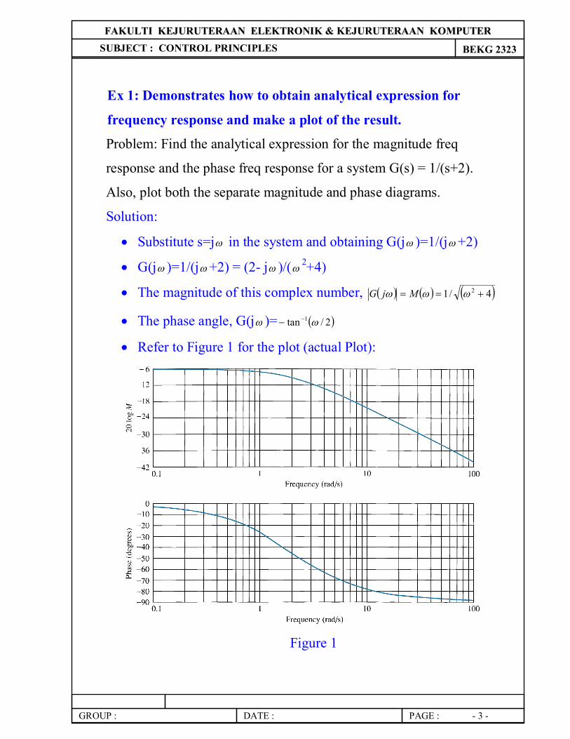
Ex 1: Demonstrates how to obtain analytical expression for

frequency response and make a plot of the result.

Problem: Find the analytical expression for the magnitude freq

response and the phase freq response for a system G(s) = 1/(s+2).

Also, plot both the separate magnitude and phase diagrams.

Solution:

Substitute s=j in the system and obtaining G(j )=1/(j+2)

G(j )=1/(j+2) = (2- j )/( 2+4)

The magnitude of this complex number, 4/1 2 MjG

The phase angle, G(j )= 2/tan 1

Refer to Figure 1 for the plot (actual Plot):

Figure 1



7.3 Asymptotic Approximations: Bode Plots

The log-magnitude and phase freq response curves as functions of log

are called Bode plots or Bode diagrams.

Sketching the bode plots can be simplified because they can be

approximated as sequence of straight lines.

Consider the following transfer function:

n

mn

pspspsszszszsKsG

........

21

21

Then, the magnitude frequency response is the product of the

magnitude freq response of each term, or

jsn

m

k

pspspss

zszszsKjG

)(...)()(

...)()(

21

21

Thus, if we know the magnitude response of each pole and zero term,

we can find the total magnitude response. The process can be

simplified by working with the logarithm of the magnitude since the

zero terms’ magnitude responses would be added and the pole terms’

magnitude responses subtracted, rather than, respectively, multiplied

or divided, to yield the logarithm of the total magnitude response.

Converting the magnitude response into dB, we obtain

15.10...log20log20...

log20)(log20log20)(log20

1

21

jsm pss

zszsKjG

Thus, if we knew the response of each term, the algebraic sum would

yield the total response in dB. Further, if we could make an

approximation of each term that would consist only of straight lines,

graphic addition of terms would be greatly simplified.



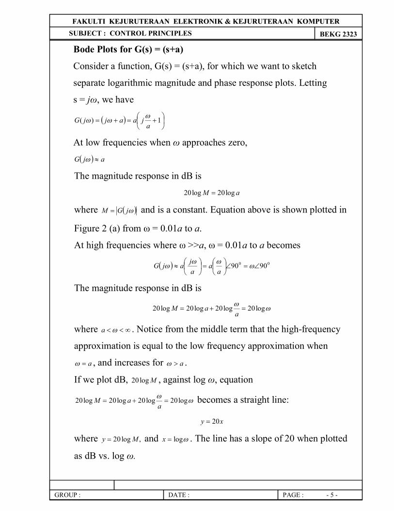
Bode Plots for G(s) = (s+a)

Consider a function, G(s) = (s+a), for which we want to sketch

separate logarithmic magnitude and phase response plots. Letting

s = jω, we have

1)(

ajaajjG

At low frequencies when ω approaches zero,

ajG

The magnitude response in dB is

aM log20log20

where jGM and is a constant. Equation above is shown plotted in

Figure 2 (a) from ω = 0.01a to a.

At high frequencies where ω >>a, ω = 0.01a to a becomes

00 9090

aa

ajajG

The magnitude response in dB is

log20log20log20log20 a

aM

where a . Notice from the middle term that the high-frequency

approximation is equal to the low frequency approximation when

a , and increases for a .

If we plot dB, Mlog20 , against log ω, equation

log20log20log20log20 a

aM becomes a straight line:

xy 20

where ,log20 My and logx . The line has a slope of 20 when plotted

as dB vs. log ω.



Figure 2 (a) & (b)

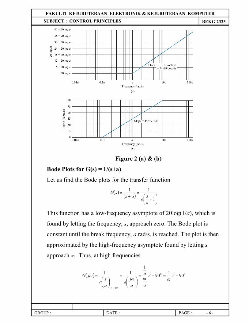
Bode Plots for G(s) = 1/(s+a)

Let us find the Bode plots for the transfer function

1

11

asaas

sG

This function has a low-frequency asymptote of 20log(1/a), which is

found by letting the frequency, s, approach zero. The Bode plot is

constant until the break frequency, a rad/s, is reached. The plot is then

approximated by the high-frequency asymptote found by letting s

approach . Thus, at high frequencies

00 90190

111

a

a

aja

asa

jG

js



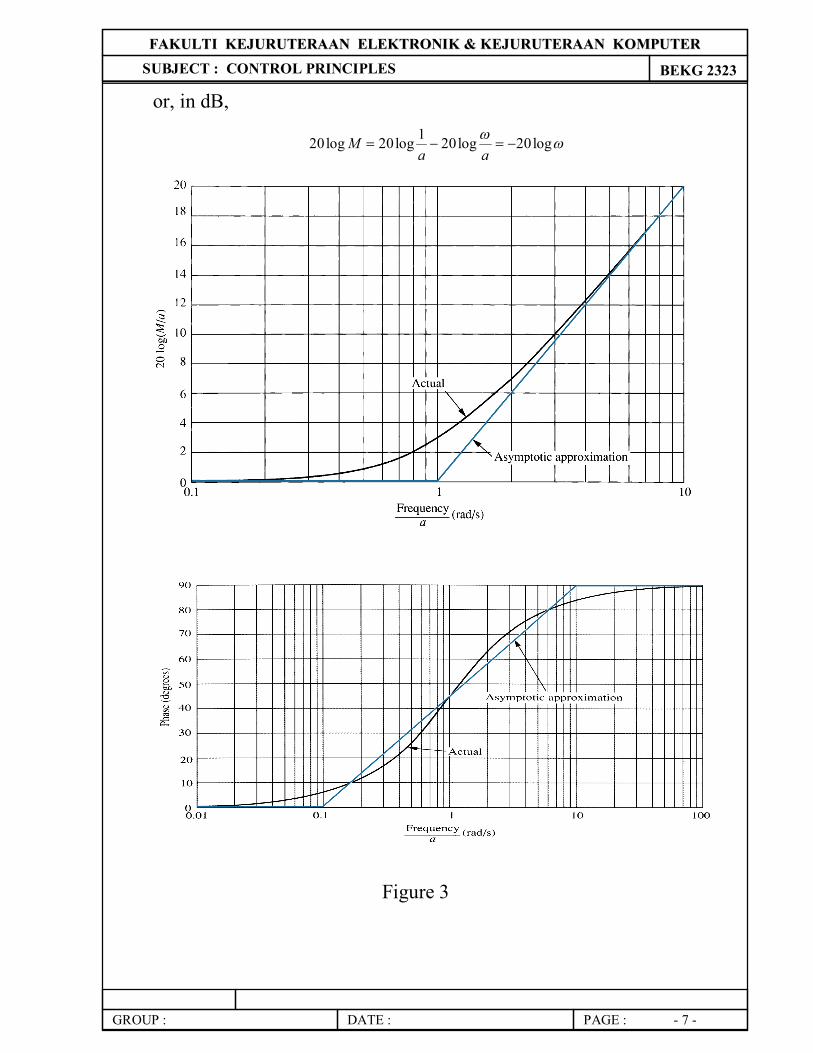
or, in dB,

log20log201log20log20 aa

M

Figure 3



Notice from the middle term that the high-frequency approximation

equals the low-frequency approximation when a , and decreases for

a . This result is similar to equation log20log20log20log20 a

aM ,

except the slope is negative rather than positive. The Bode log-

magnitude diagram will decrease at a rate of 20 dB/decade rather than

increase at a rate of 20 dB/decade after the break frequency.

The phase plot is the negative of the previous example sine the

function is the inverse. The phase begins at 00 and reaches -900 at high

frequencies, going through -450 at the break frequency. Both the Bode

normalized and scaled log-magnitude and phase plot are shown in

Figure 4 (d).

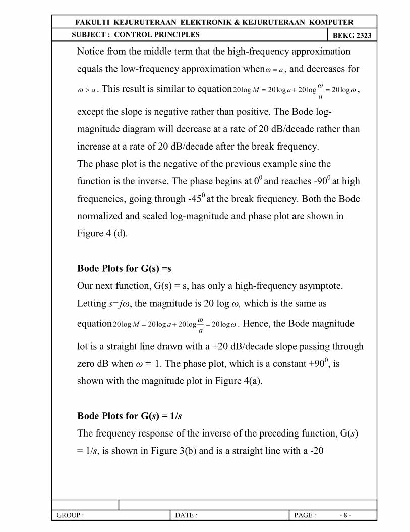
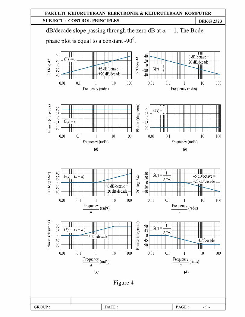
Bode Plots for G(s) =s

Our next function, G(s) = s, has only a high-frequency asymptote.

Letting s=jω, the magnitude is 20 log ω, which is the same as

equation log20log20log20log20 a

aM . Hence, the Bode magnitude

lot is a straight line drawn with a +20 dB/decade slope passing through

zero dB when ω = 1. The phase plot, which is a constant +900, is

shown with the magnitude plot in Figure 4(a).

Bode Plots for G(s) = 1/s

The frequency response of the inverse of the preceding function, G(s)

= 1/s, is shown in Figure 3(b) and is a straight line with a -20



dB/decade slope passing through the zero dB at ω = 1. The Bode

phase plot is equal to a constant -900.

Figure 4



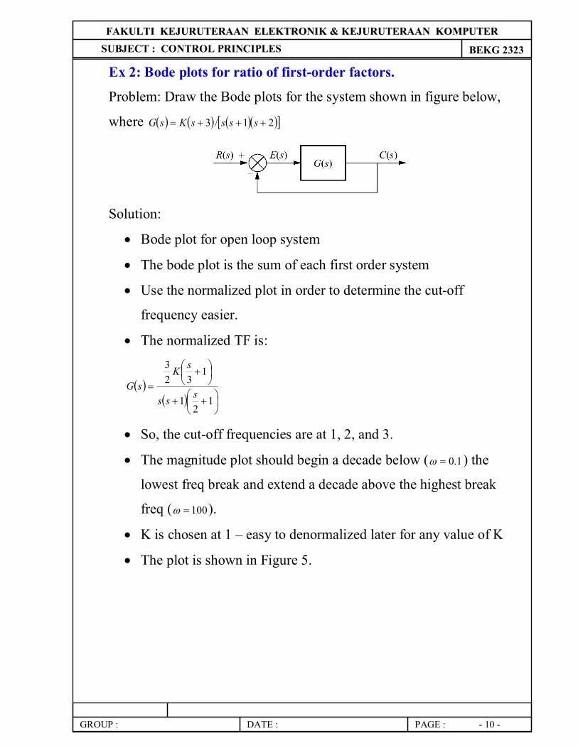
Ex 2: Bode plots for ratio of first-order factors.

Problem: Draw the Bode plots for the system shown in figure below,

where 21/3 ssssKsG

Solution:

Bode plot for open loop system

The bode plot is the sum of each first order system

Use the normalized plot in order to determine the cut-off

frequency easier.

The normalized TF is:

1

21

132

3

sss

sKsG

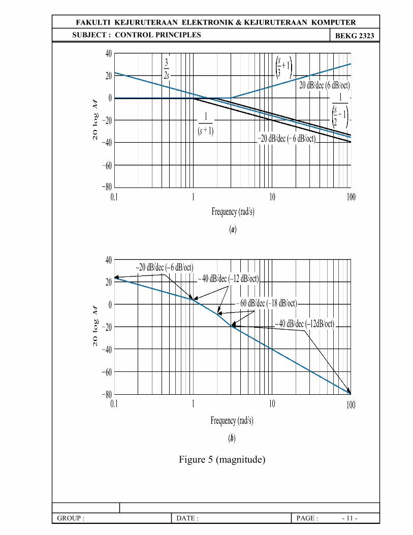
So, the cut-off frequencies are at 1, 2, and 3.

The magnitude plot should begin a decade below ( 1.0 ) the

lowest freq break and extend a decade above the highest break

freq ( 100 ).

K is chosen at 1 – easy to denormalized later for any value of K

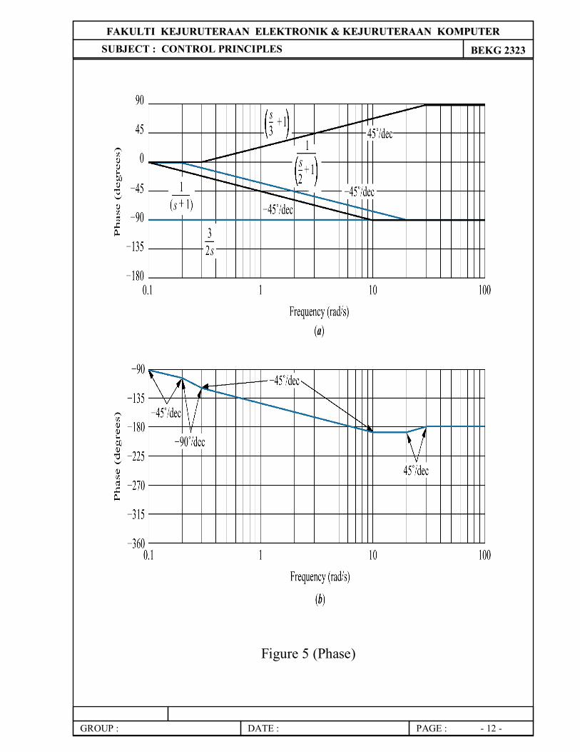
The plot is shown in Figure 5.



Figure 5 (magnitude)



Figure 5 (Phase)



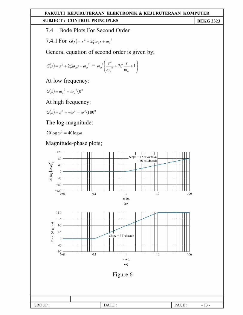
7.4 Bode Plots For Second Order

7.4.1 For 22 2 nnsssG

General equation of second order is given by;

22 2 nn sssG =

122

22

nnn

ss

At low frequency:

022 0 nnsG

At high frequency: 0222 180 ssG

The log-magnitude:

log40log20 2

Magnitude-phase plots;

Figure 6



7.4.2 For 22 2/1 nn sssG

Magnitude-phase plots:

Reverse of the plots in section 7.4.1.

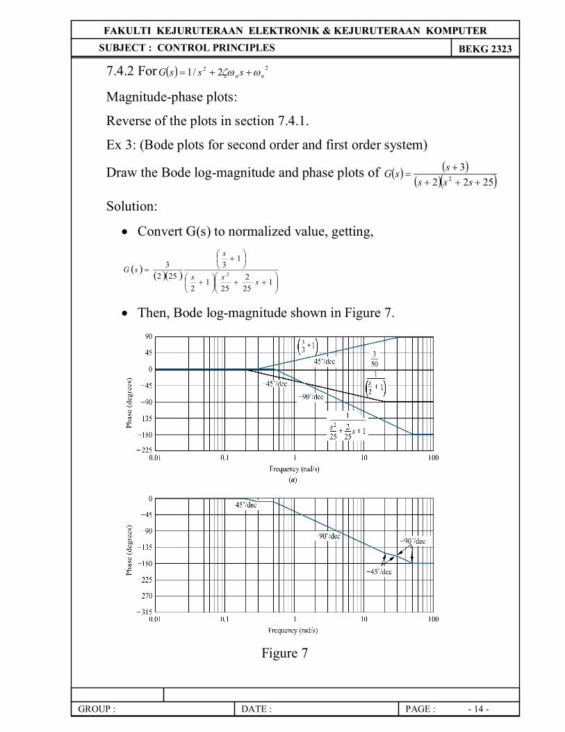
Ex 3: (Bode plots for second order and first order system)

Draw the Bode log-magnitude and phase plots of 2522

32

sss

ssG

Solution:

Convert G(s) to normalized value, getting,

1

252

251

2

13

2523

2

sss

s

sG

Then, Bode log-magnitude shown in Figure 7.

Figure 7



7.5 Stability, Gain Margin, and Phase Margin via Bode Plots

7.5.1 Determining Stability

The specification below should be get in order to ensure the stability

of the system using Bode Plots

The closed loop system will be stable if the frequency response

has a gain less than unity when phase is 1800.

Ex 4:

Use Bode Plots to determine the range of K within which the unity

feedback system is stable. Let 542

sssKsG

Solution:

Convert G(s) to normalized value, yields,

1

51

41

2

140 sssKsG

Choose K = 40 in order to start the plots at 0db

Break frequency at 2, 4, and 5

Lowest frequency, 01.0 ; Highest frequency, 100

Plots,



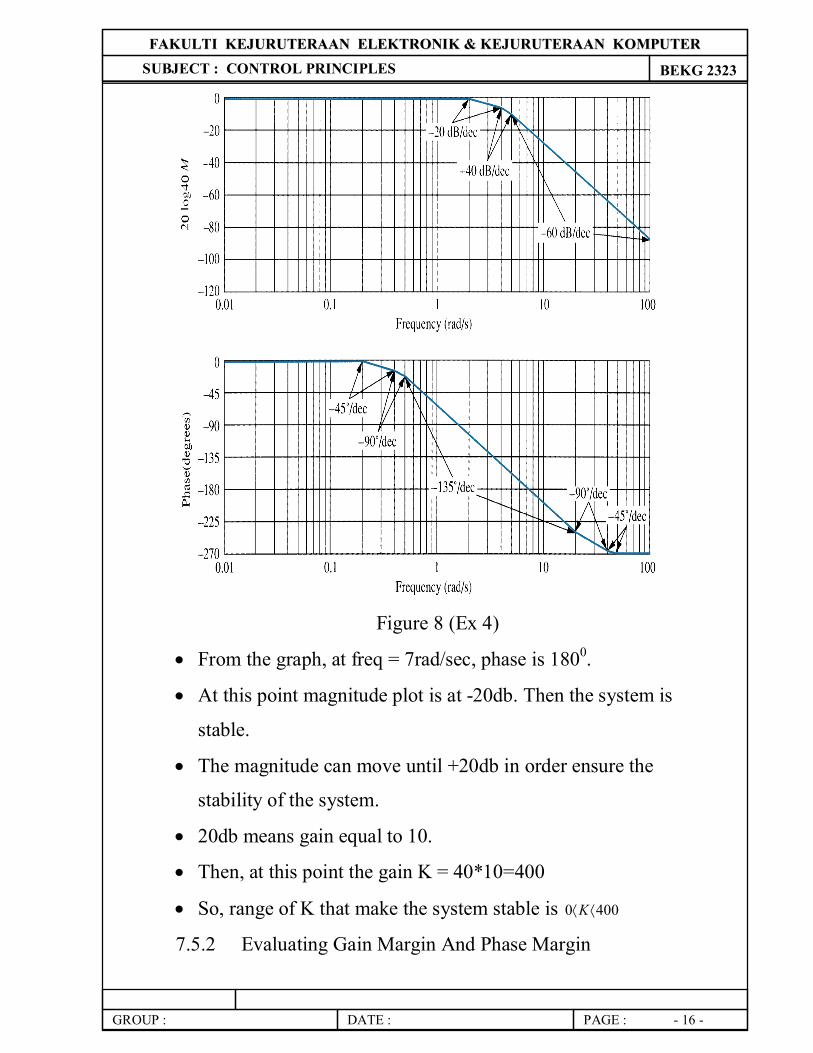
Figure 8 (Ex 4)

From the graph, at freq = 7rad/sec, phase is 1800.

At this point magnitude plot is at -20db. Then the system is

stable.

The magnitude can move until +20db in order ensure the

stability of the system.

20db means gain equal to 10.

Then, at this point the gain K = 40*10=400

So, range of K that make the system stable is 4000 K

7.5.2 Evaluating Gain Margin And Phase Margin



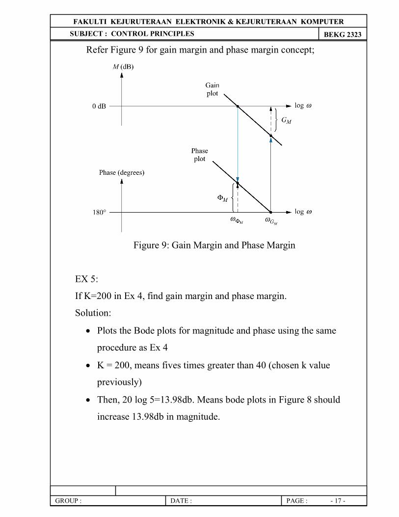
Refer Figure 9 for gain margin and phase margin concept;

Figure 9: Gain Margin and Phase Margin

EX 5:

If K=200 in Ex 4, find gain margin and phase margin.

Solution:

Plots the Bode plots for magnitude and phase using the same

procedure as Ex 4

K = 200, means fives times greater than 40 (chosen k value

previously)

Then, 20 log 5=13.98db. Means bode plots in Figure 8 should

increase 13.98db in magnitude.



Therefore, to find gain margin look at phase plot and the freq

when phase is 180o. At this freq, determine from the magnitude

plot how much the gain can be increased before reaching 0dB.

From Figure 8, the phase angle is 180o at approximately 7 rad/s.

On the magnitude plot, the gain is -20 dB + 13.98 dB = -6.02 dB.

Thus, the gain margin is 6.02 dB.

For phase margin, refer freq at magnitude plot where the gain is

0 dB. At this freq, look on the phase plot to find the difference

between the phase and 180o. The difference is phase margin.

From Figure 8, remember that the magnitude plot is 13.98 dB

lower than actual plot, the 0 dB crossing (-13.98 dB for the

normalized plot shown in Figure 8) occurs at 5.5 rad/s.

At this freq, the phase angle is -165o. Thus, the phase margin is

-165-(-180) = 15o

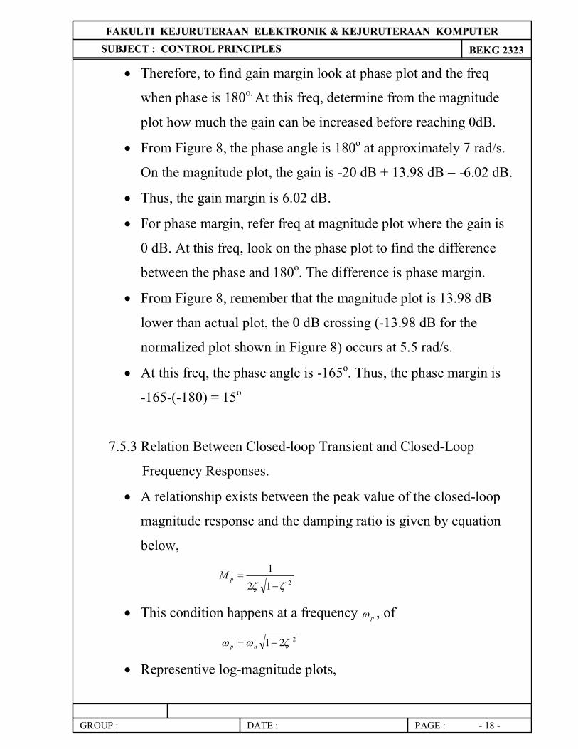
7.5.3 Relation Between Closed-loop Transient and Closed-Loop

Frequency Responses.

A relationship exists between the peak value of the closed-loop

magnitude response and the damping ratio is given by equation

below,

212

1

pM

This condition happens at a frequency p , of

221 np

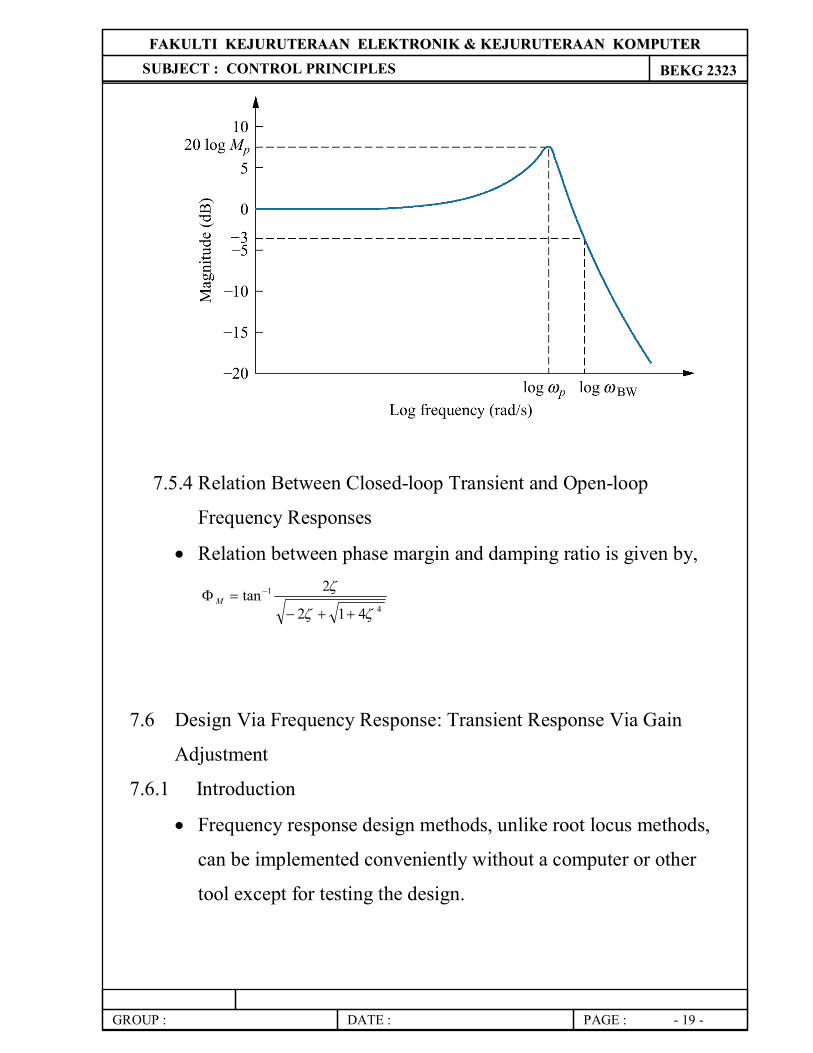
Representive log-magnitude plots,



7.5.4 Relation Between Closed-loop Transient and Open-loop

Frequency Responses

Relation between phase margin and damping ratio is given by,

4

1

412

2tan

M

7.6 Design Via Frequency Response: Transient Response Via Gain

Adjustment

7.6.1 Introduction

Frequency response design methods, unlike root locus methods,

can be implemented conveniently without a computer or other

tool except for testing the design.



The bode plots can be designed easily using asymptotic

approximations and gain can be read from there.

7.6.2 Gain Adjustment

From previous discussion the phase margin is relates to the

damping ratio (equivalently percent overshoot).

Thus, any varying in phase margin will result on varying the

percent overshoot.

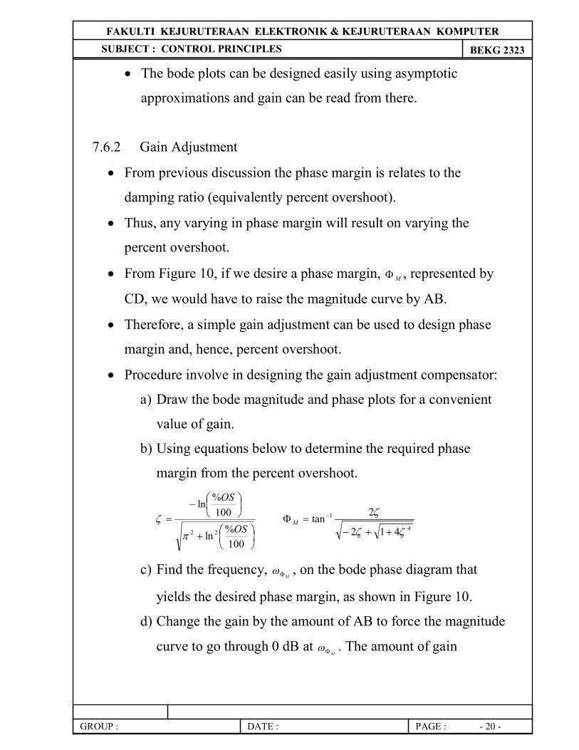
From Figure 10, if we desire a phase margin, M , represented by

CD, we would have to raise the magnitude curve by AB.

Therefore, a simple gain adjustment can be used to design phase

margin and, hence, percent overshoot.

Procedure involve in designing the gain adjustment compensator:

a) Draw the bode magnitude and phase plots for a convenient

value of gain.

b) Using equations below to determine the required phase

margin from the percent overshoot.

100%ln

100%ln

22 OS

OS

4

1

412

2tan

M

c) Find the frequency, M , on the bode phase diagram that

yields the desired phase margin, as shown in Figure 10.

d) Change the gain by the amount of AB to force the magnitude

curve to go through 0 dB at M . The amount of gain



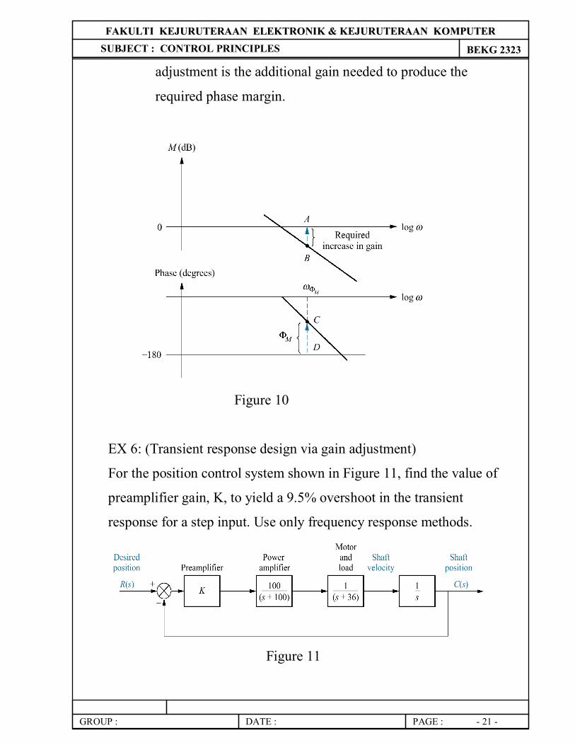
adjustment is the additional gain needed to produce the

required phase margin.

Figure 10

EX 6: (Transient response design via gain adjustment)

For the position control system shown in Figure 11, find the value of

preamplifier gain, K, to yield a 9.5% overshoot in the transient

response for a step input. Use only frequency response methods.

Figure 11



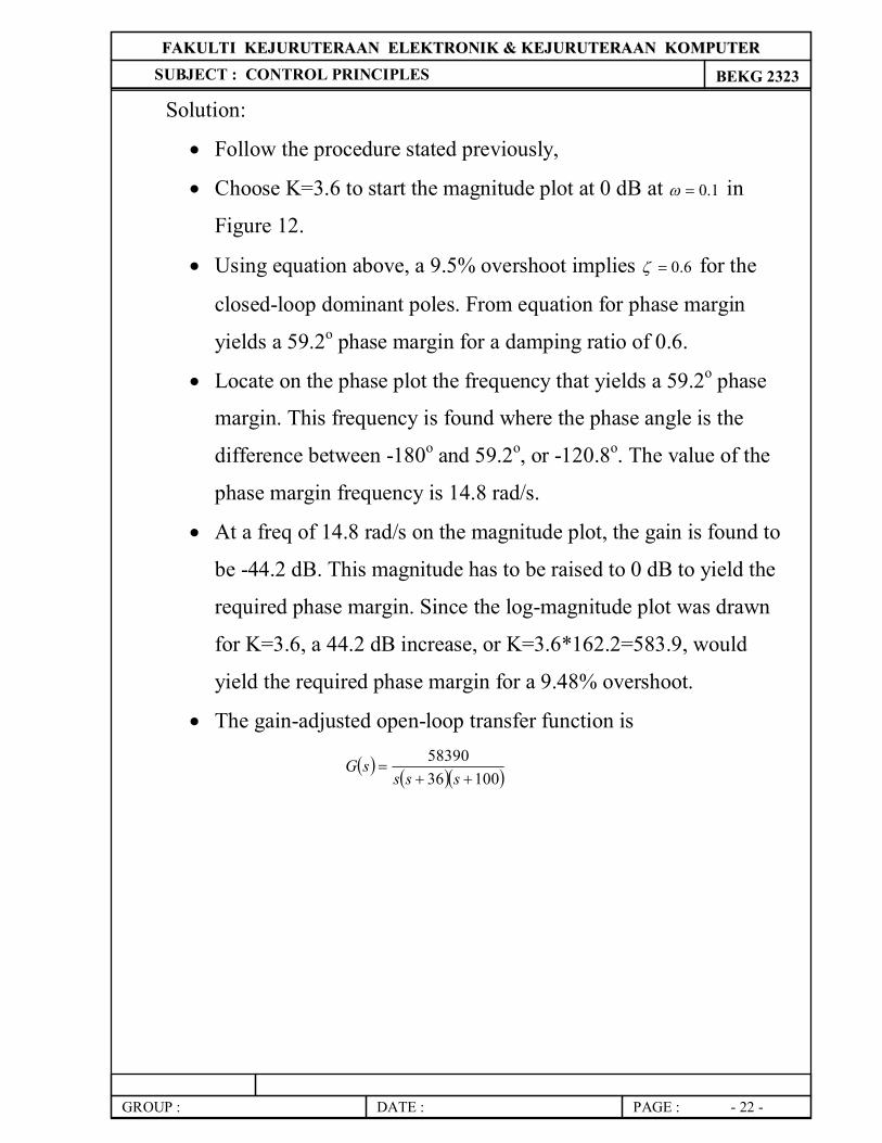
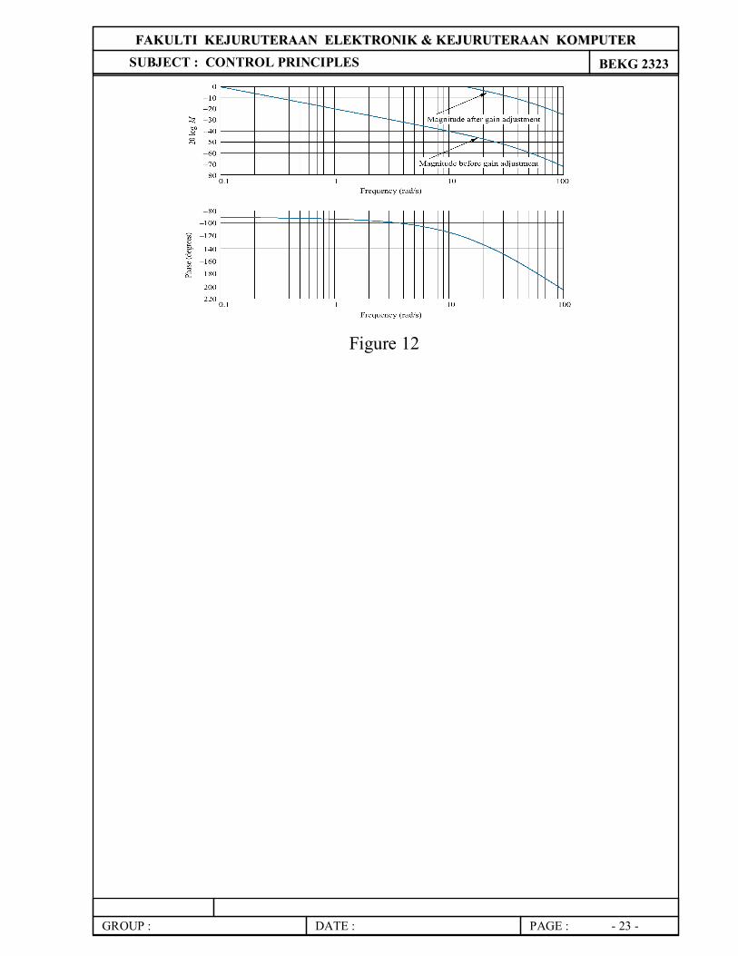
Solution:

Follow the procedure stated previously,

Choose K=3.6 to start the magnitude plot at 0 dB at 1.0 in

Figure 12.

Using equation above, a 9.5% overshoot implies 6.0 for the

closed-loop dominant poles. From equation for phase margin

yields a 59.2o phase margin for a damping ratio of 0.6.

Locate on the phase plot the frequency that yields a 59.2o phase

margin. This frequency is found where the phase angle is the

difference between -180o and 59.2o, or -120.8o. The value of the

phase margin frequency is 14.8 rad/s.

At a freq of 14.8 rad/s on the magnitude plot, the gain is found to

be -44.2 dB. This magnitude has to be raised to 0 dB to yield the

required phase margin. Since the log-magnitude plot was drawn

for K=3.6, a 44.2 dB increase, or K=3.6*162.2=583.9, would

yield the required phase margin for a 9.48% overshoot.

The gain-adjusted open-loop transfer function is

1003658390

ssssG



Figure 12

Documents

FAKULTI KEJURUTERAAN ELEKTRONIK & KEJURUTERAAN KOMPUTER ...myweb.utem.edu.my/myweb/amat/downloads/BEKG2323/Chapter7.pdf · fakulti kejuruteraan elektronik & kejuruteraan komputer