Embed Size (px)
Citation preview
Future Demand and Energy Outlook(2009 – 2029)
Future Demand and Energy Outlook (2009 – 2029)
Table of Contents
Executive Summary 1
1.0 Introduction 3
2.0 Economic Outlook 4
2.1 Alberta’s GDP Growth 4
2.2 Alberta’s Population Growth 6
2.3 Oilsands Production Growth 7
3.0 Methodology 9
3.1 AESO Methodology Diagram 10
3.2 Industrial (without Oilsands) Customer Sector 11
3.3 Oilsands Customer Sector 13
3.4 Commercial Customer Sector 15
3.5 Residential Customer Sector 17
3.6 Farm Customer Sector 19
3.7 Historical Growth and Decrease in 10 Ten Industrial Sites 21
4.0 Forecast Results 24
4.1 Provincial Results – AIL Forecast 25
4.2 Provincial Results – AIES Forecast with Behind-the-Fence (BTF) Load Estimation 27
4.3 Provincial Results – Demand Tariff Service (DTS) Energy 29
4.4 Forecast Results for Bulk Planning Purposes 29
4.5 Forecast Results for Regional Planning Purposes 32
5.0 Other Load Forecasting Considerations 36
5.1 Demand Responsive Load and Conservation 36
5.2 Composition of Load 38
5.3 Distributed Generation 39
5.4 Environmental Costs 39
5.5 Challenges on the Horizon 40
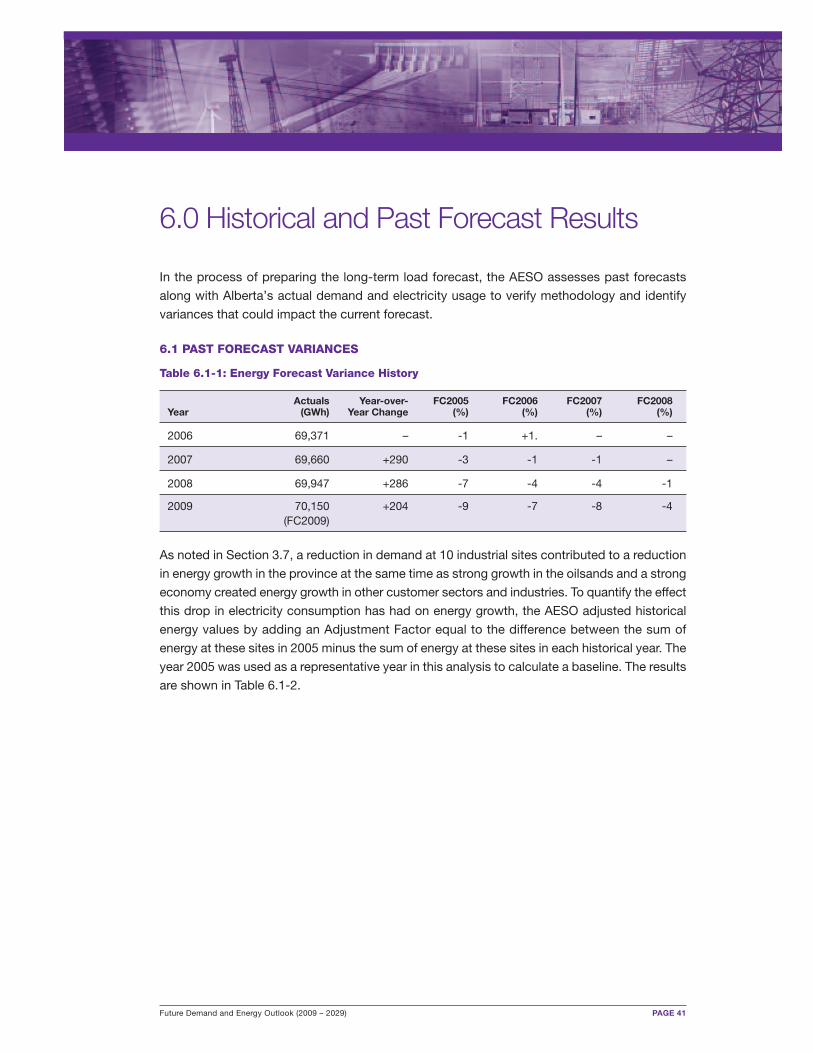
6.0 Historical and Past Forecast Results 41
6.1 Past Forecast Variances 41
Future Demand and Energy Outlook (2009 – 2029)
Appendix A: Confidence Band Intervals for the Future Demand and Energy Outlook (2009 – 2029) 43
Executive Summary 43
1.0 Introduction 44
2.0 Monte Carlo Analysis 45
2.1 Industrial (without Oilsands) Customer Sector 46
2.2 Oilsands Customer Sector 47
2.3 Commercial Customer Sector 48
2.4 Residential Customer Sector 49
2.5 Farm Customer Sector 50
3.0 Total Energy and Peak Demand 51
3.1 Monte Carlo Results 51
List of Reference Documents 56
Glossary 57
Figures
Figure 2.1-1: Changes in GDP 5
Figure 2.2-1: Population Growth in Alberta 6
Figure 2.2-2: Alberta Population 6
Figure 2.3-1: Oilsands Bitumen Production Forecast 8
Figure 2.3-2: Synthetic Crude Oil Production Forecast 8
Figure 3.0-1: Customer Sector as Percentage of Total Energy (2008) 9
Figure 3.1-1: AESO Load Forecast Methodology Flow Diagram 10
Figure 3.2-1: Historical Industrial (without Oilsands) Energy 11
Figure 3.2-2: Industrial End Use as Percentage of Total Industrial (2006) 12
Figure 3.2-3: Industrial (without Oilsands) Energy Intensity 12
Figure 3.2-4: Industrial (without Oilsands) Energy Forecast 13
Figure 3.3-1: Oilsands Energy Intensity 14
Figure 3.3-2: Oilsands Energy Forecast 14
Figure 3.4-1: Historical Commercial Energy Usage 15
Figure 3.4-2: Commercial Energy and Alberta GDP 15
Figure 3.4-3: Commercial Energy Intensity 16
Figure 3.4-4: Commercial Energy Forecast 16
Figure 3.5-1: Historical Residential Energy Use 17
Figure 3.5-2: Residential Energy Use Per Capita 18
Figure 3.5-3: Residential Energy Forecast 18
Figure 3.6-1: Historical Farm Energy 19
Future Demand and Energy Outlook (2009 – 2029)
Figure 3.6-2: Agricultural Land in Alberta 20
Figure 3.6-3: Farm Energy Forecast 20
Figure 3.7-1: Historical Energy of 10 Industrial Firms 22
Figure 3.7-2: Historical AIL Energy with Adjustment Factor 22
Figure 3.7-3: Historical and Forecast AIL Energy Growth 23
Figure 3.7-4: Alberta GDP Growth Forecasts 23
Figure 4.4-1: Region Demand at Time of Winter AIL Peak Demand 30
Figure 4.4-2: Region Demand at Time of Summer AIL Peak Demand 31
Figure 4.5-1: Grouping of Areas for Regional Planning Purposes 33
Appendix: Figure 2.1-1: Industrial (without Oilsands) Sector Confidence Intervals 46
Appendix: Figure 2.2-1: Oilsands Sector Confidence Intervals 47
Appendix: Figure 2.3-1: Commercial Sector Confidence Intervals 48
Appendix: Figure 2.4-1: Residential Sector Confidence Intervals 49
Appendix: Figure 2.5-1: Farm Sector Confidence Intervals 50
Appendix: Figure 3.1-1: AIL Energy Confidence Intervals 51
Appendix: Figure 3.1-2: AIL Winter Peak Demand Confidence Intervals 52
Tables
Table 3.3-1: Energy Intensities 13
Table 4.0-1: Alberta Energy Sales to AIL Energy (GWh) 24
Table 4.1-1: AIL Winter Peak Demand 25
Table 4.1-2: AIL Summer Peak Demand 25
Table 4.1-3: AIL Annual Energy 26
Table 4.2-1: AIES Winter Peak Demand 27
Table 4.2-2: AIES Summer Peak Demand 27
Table 4.2-3: AIES Annual Energy 28
Table 4.3-1: DTS Annual Energy 29
Table 4.5-1: Coincident Peak Demand (MW) for South Region 34
Table 4.5-2: Coincident Peak Demand (MW) for Calgary Region 34
Table 4.5-3: Coincident Peak Demand (MW) for Central Region 34
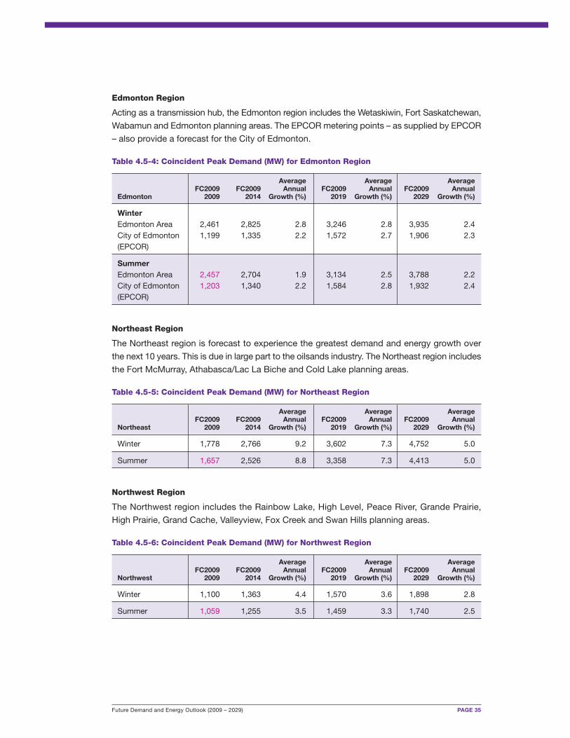
Table 4.5-4: Coincident Peak Demand (MW) for Edmonton Region 35
Table 4.5-5: Coincident Peak Demand (MW) for Northeast Region 35
Table 4.5-6: Coincident Peak Demand (MW) for Northwest Region 35
Table 6.1-1: Energy Forecast Variance History 41
Table 6.1-2: Historical Energy with Adjustments for 10 Industrial Sites’ Reduction in Load 42
Table 6.1-3: Peak Forecast Variance History 42
Appendix: Table 3.1-1: AIL Energy Confidence Intervals 54
Appendix: Table 3.1-2: AIL Winter Peak Demand Confidence Intervals 55
Future Demand and Energy Outlook (2009 – 2029) PAGE 1
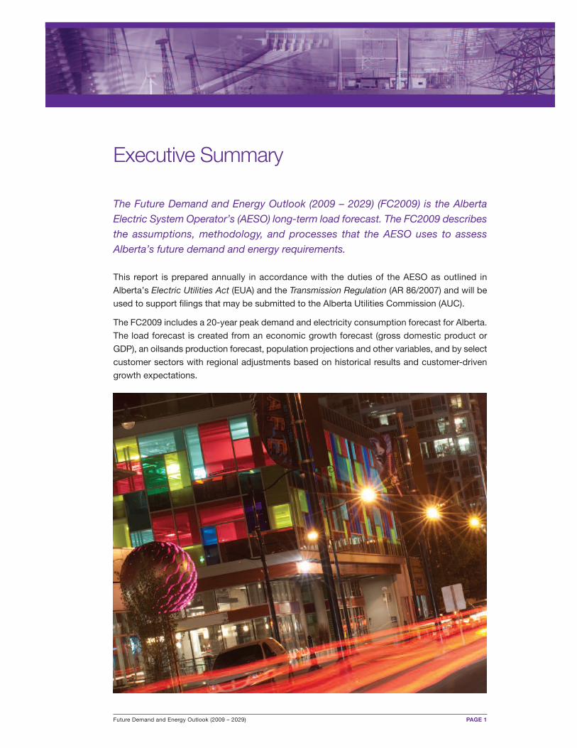
Executive Summary
The Future Demand and Energy Outlook (2009 – 2029) (FC2009) is the AlbertaElectric System Operator’s (AESO) long-term load forecast. The FC2009 describesthe assumptions, methodology, and processes that the AESO uses to assessAlberta’s future demand and energy requirements.
This report is prepared annually in accordance with the duties of the AESO as outlined in
Alberta’s Electric Utilities Act (EUA) and the Transmission Regulation (AR 86/2007) and will be
used to support filings that may be submitted to the Alberta Utilities Commission (AUC).
The FC2009 includes a 20-year peak demand and electricity consumption forecast for Alberta.
The load forecast is created from an economic growth forecast (gross domestic product or
GDP), an oilsands production forecast, population projections and other variables, and by select
customer sectors with regional adjustments based on historical results and customer-driven
growth expectations.
PAGE 2 Future Demand and Energy Outlook (2009 – 2029)
In the past five years (2003 – 2008) Alberta internal load (AIL) peak demand has grown by an
average of 206 megawatts (MW) (1.5 per cent) per year from 8,967 MW to 9,806 MW (an overall
increase of 9.4 per cent). AIL is the sum of all electricity sales (residential, commercial, industrial
and farm), losses (both transmission and distribution) and behind-the-fence load (BTF). Electricity
consumption has grown by an average of 2.2 per cent per year from 62,716 gigawatt hours
(GWh) to 69,947 GWh for the same period.
Historical energy growth in the last three years has been driven by oilsands projects and a
booming oil and gas industry. However, over the past three years, the forestry, pulp and paper,
and chemical industries have been negatively impacted by rising labour and other costs and
lowered demand. As a result, a small number of industrial sites have either shut down or
drastically reduced production, which has impacted overall energy and demand growth. The
AESO has evaluated and researched the size and impact of these closures or reductions and
determined that in the long term they are not material to the forecast. For this outlook, the AESO
has not selected specific sites where shutdowns or reductions in load may occur in the future
unless a specific customer request has been made.
The AESO forecasts AIL peak demand to grow by an average 3.3 per cent per year for the period
from 2009 to 2029. Electricity consumption (energy) is also expected to grow by 3.2 per cent
per year for the same period. The primary driver of this growth is related to growth in the oilsands
and associated development.
The global financial meltdown of late 2008 and the subsequent worldwide economic recession
have negatively affected economic growth in Alberta. However, it is expected that Alberta’s
economy will recover and return to growth in 2010. Overall, long-run fundamentals remain
robust with investments and developments in the oilsands expected to help drive strong
economic growth over the next decade.
In addition to reporting the detailed forecast results, this report includes a summary of the
AESO’s load forecasting methodology. The energy and demand forecast is prepared based on
an examination of five sectors: industrial without oilsands, oilsands, commercial, residential
and farm. The results are organized by the AESO’s five bulk transmission planning regions and
six regional transmission planning regions.
The FC2009 concludes with a discussion of the challenges faced in preparing a load forecast
for Alberta.
Future Demand and Energy Outlook (2009 – 2029) PAGE 3
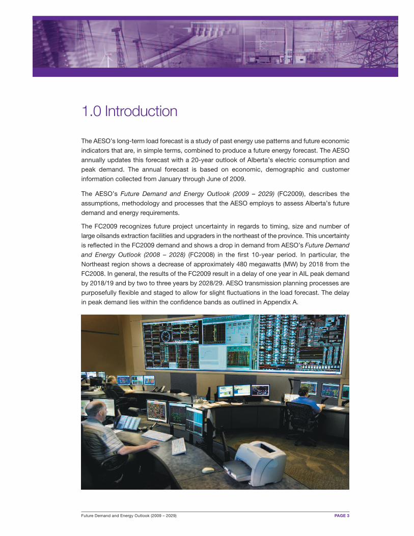
1.0 Introduction
The AESO’s long-term load forecast is a study of past energy use patterns and future economic
indicators that are, in simple terms, combined to produce a future energy forecast. The AESO
annually updates this forecast with a 20-year outlook of Alberta’s electric consumption and
peak demand. The annual forecast is based on economic, demographic and customer
information collected from January through June of 2009.
The AESO’s Future Demand and Energy Outlook (2009 – 2029) (FC2009), describes the
assumptions, methodology and processes that the AESO employs to assess Alberta’s future
demand and energy requirements.
The FC2009 recognizes future project uncertainty in regards to timing, size and number of
large oilsands extraction facilities and upgraders in the northeast of the province. This uncertainty
is reflected in the FC2009 demand and shows a drop in demand from AESO’s Future Demand
and Energy Outlook (2008 – 2028) (FC2008) in the first 10-year period. In particular, the
Northeast region shows a decrease of approximately 480 megawatts (MW) by 2018 from the
FC2008. In general, the results of the FC2009 result in a delay of one year in AIL peak demand
by 2018/19 and by two to three years by 2028/29. AESO transmission planning processes are
purposefully flexible and staged to allow for slight fluctuations in the load forecast. The delay
in peak demand lies within the confidence bands as outlined in Appendix A.
2.0 Economic Outlook
The foundation for the AESO’s electricity demand and energy forecast is Alberta’s economic
outlook, which continues to be strong according to The Conference Board of Canada’s long-term
economic forecast (Provincial Outlook Long-term Forecast 2009, published in April 2009). As well,
estimates of investment and growth in the oilsands sector will continue to power Alberta’s
economy in the next 15 years according to the Canadian Association of Petroleum Producers
(CAPP) (Crude Oil Forecast, Markets & Pipeline Expansions - June 2009; Moderate Forecast).
The AESO’s economic outlook is developed by reviewing and using information and analysis
from The Conference Board of Canada, CAPP and Statistics Canada.
The key factor driving the Alberta economy continues to be investment in the development of
oilsands, which is largely driven by oil demand and world crude oil prices. This investment
creates jobs and economic activity that, in general, will lead to a continuation of increases in
annual electricity use.
2.1 ALBERTA’S GDP GROWTH
Gross domestic product (GDP), a measure of economic activity, is a function of consumer
spending, private and public investment, and exports and imports. Declining crude oil and
natural gas prices resulting from the world recession have negatively impacted the energy-
dependent Alberta economy. Consequently, the province entered into a recession and
experienced negative economic growth in 2009.
However, it is generally expected the Alberta economy will begin to rebound in 2010 followed
by several years of strong growth. This strong growth is expected to be primarily driven by
investments in the oilsands sector. Increasing world demand for crude oil, especially from
emerging countries, combined with difficulty in increasing supply from traditional oil exporting
regions is likely to increase demand for oilsands bitumen. Oilsands investment will spur
additional economic activity in supporting industries and will generally benefit the province’s
economy. In addition, job creation will encourage immigration to Alberta.
Economic growth, as measured by provincial GDP, is expected to be strong in the coming
decade despite an expected economic contraction in 2009. GDP growth from 2010 to 2020 is
expected to range from 2.1 to 5.5 per cent annually. According to The Conference Board of
Canada’s Provincial Outlook Spring 2009, GDP is forecast to decline by 2.4 per cent in 2009
and increase by 2.9 per cent in 2010.
PAGE 4 Future Demand and Energy Outlook (2009 – 2029)
Future Demand and Energy Outlook (2009 – 2029) PAGE 5
Long-run economic growth in Alberta will be somewhat tempered by labour constraints and
increasing construction and materials costs, as well as increasing living costs and under-
developed infrastructure.
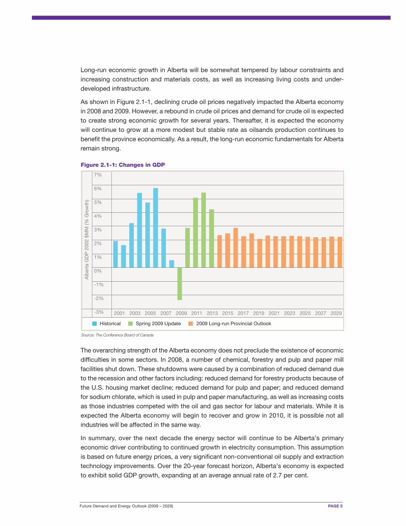
As shown in Figure 2.1-1, declining crude oil prices negatively impacted the Alberta economy
in 2008 and 2009. However, a rebound in crude oil prices and demand for crude oil is expected
to create strong economic growth for several years. Thereafter, it is expected the economy
will continue to grow at a more modest but stable rate as oilsands production continues to
benefit the province economically. As a result, the long-run economic fundamentals for Alberta
remain strong.
The overarching strength of the Alberta economy does not preclude the existence of economic
difficulties in some sectors. In 2008, a number of chemical, forestry and pulp and paper mill
facilities shut down. These shutdowns were caused by a combination of reduced demand due
to the recession and other factors including: reduced demand for forestry products because of
the U.S. housing market decline; reduced demand for pulp and paper; and reduced demand
for sodium chlorate, which is used in pulp and paper manufacturing, as well as increasing costs
as those industries competed with the oil and gas sector for labour and materials. While it is
expected the Alberta economy will begin to recover and grow in 2010, it is possible not all
industries will be affected in the same way.
In summary, over the next decade the energy sector will continue to be Alberta’s primary
economic driver contributing to continued growth in electricity consumption. This assumption
is based on future energy prices, a very significant non-conventional oil supply and extraction
technology improvements. Over the 20-year forecast horizon, Alberta’s economy is expected
to exhibit solid GDP growth, expanding at an average annual rate of 2.7 per cent.
7%
6%
5%
4%
3%
2%
1%
0%
-1%
-2%
-3%
Source: The Conference Board of Canada
2001
Alb
erta
GD
P 2
002
$MM
(% G
row
th)
Historical
2003 2005 2007 2009 2011 2013 2015 2017 2019 2021 2023 2025 2027 2029
Spring 2009 Update 2009 Long-run Provincial Outlook
Figure 2.1-1: Changes in GDP
PAGE 6 Future Demand and Energy Outlook (2009 – 2029)
2.2 ALBERTA’S POPULATION GROWTH
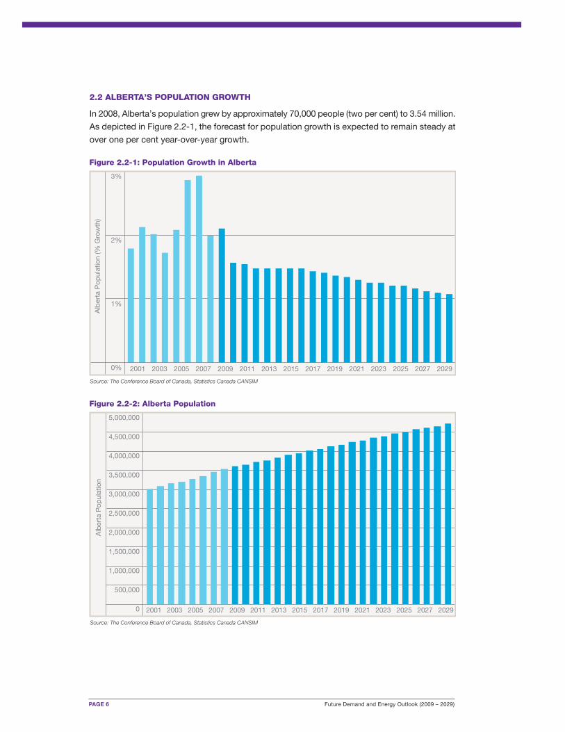
In 2008, Alberta’s population grew by approximately 70,000 people (two per cent) to 3.54 million.
As depicted in Figure 2.2-1, the forecast for population growth is expected to remain steady at
over one per cent year-over-year growth.
3%
2%
1%
0%
Source: The Conference Board of Canada, Statistics Canada CANSIM
2001 2003 2005 2007 2009 2011 2013 2015 2017 2019 2021 2023 2025 2027 2029
Figure 2.2-1: Population Growth in Alberta
Alb
erta
Pop
ulat
ion
(% G
row
th)
5,000,000
4,500,000
4,000,000
3,500,000
3,000,000
2,500,000
2,000,000
1,500,000
1,000,000
500,000
0
Source: The Conference Board of Canada, Statistics Canada CANSIM
2001 2003 2005 2007 2009 2011 2013 2015 2017 2019 2021 2023 2025 2027 2029
Figure 2.2-2: Alberta Population
Alb
erta
Pop
ulat
ion
Future Demand and Energy Outlook (2009 – 2029) PAGE 7
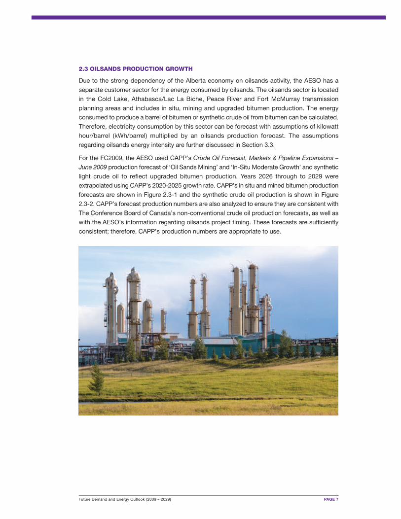
2.3 OILSANDS PRODUCTION GROWTH
Due to the strong dependency of the Alberta economy on oilsands activity, the AESO has a
separate customer sector for the energy consumed by oilsands. The oilsands sector is located
in the Cold Lake, Athabasca/Lac La Biche, Peace River and Fort McMurray transmission
planning areas and includes in situ, mining and upgraded bitumen production. The energy
consumed to produce a barrel of bitumen or synthetic crude oil from bitumen can be calculated.
Therefore, electricity consumption by this sector can be forecast with assumptions of kilowatt
hour/barrel (kWh/barrel) multiplied by an oilsands production forecast. The assumptions
regarding oilsands energy intensity are further discussed in Section 3.3.
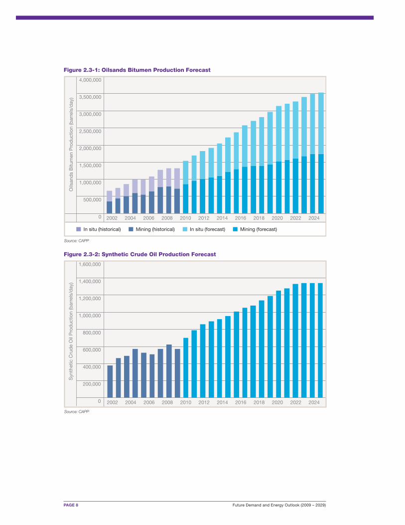
For the FC2009, the AESO used CAPP’s Crude Oil Forecast, Markets & Pipeline Expansions –
June 2009 production forecast of ‘Oil Sands Mining’ and ‘In-Situ Moderate Growth’ and synthetic
light crude oil to reflect upgraded bitumen production. Years 2026 through to 2029 were
extrapolated using CAPP’s 2020-2025 growth rate. CAPP’s in situ and mined bitumen production
forecasts are shown in Figure 2.3-1 and the synthetic crude oil production is shown in Figure
2.3-2. CAPP’s forecast production numbers are also analyzed to ensure they are consistent with
The Conference Board of Canada’s non-conventional crude oil production forecasts, as well as
with the AESO’s information regarding oilsands project timing. These forecasts are sufficiently
consistent; therefore, CAPP’s production numbers are appropriate to use.
PAGE 8 Future Demand and Energy Outlook (2009 – 2029)
4,000,000
3,500,000
3,000,000
2,500,000
2,000,000
1,500,000
1,000,000
500,000
0
Source: CAPP
2002 2004 2006 2008 2010 2012 2014 2016 2018 2020 2022 2024
In situ (historical) Mining (historical) In situ (forecast) Mining (forecast)
Figure 2.3-1: Oilsands Bitumen Production ForecastO
ilsan
ds
Bitu
men
Pro
duc
tion
(bar
rels
/day
)
1,600,000
1,400,000
1,200,000
1,000,000
800,000
600,000
400,000
200,000
0
Source: CAPP
Syn
thet
ic C
rud
e O
il P
rod
uctio
n (b
arre
ls/d
ay)
2002 2004 2006 2008 2010 2012 2014 2016 2018 2020 2022 2024
Figure 2.3-2: Synthetic Crude Oil Production Forecast
Future Demand and Energy Outlook (2009 – 2029) PAGE 9
3.0 Methodology
The AESO primarily uses an econometric approach to estimating future demand and electricity
usage. This methodology provides a consistent approach to load forecasting through the use
of a combination of fitted statistical models, historical data, third-party economic forecasts and
customer-specific information.
The long-term load forecast is developed by considering the five categories listed below:
� Industrial without Oilsands
� Oilsands
� Commercial
� Residential
� Farm
A high-level overview of the AESO’s long-term load forecasting methodology is found in
Figure 3.1-1 and details for each sector are discussed in the sections that follow.
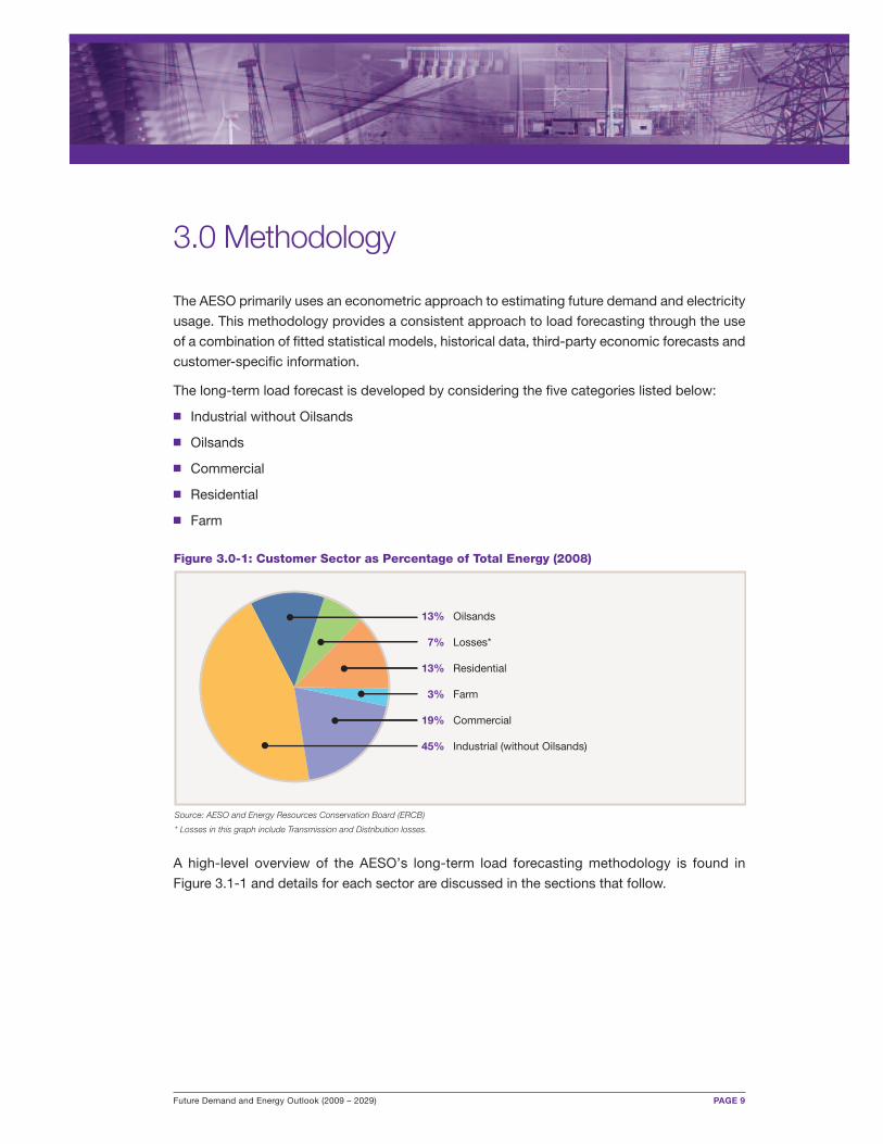
Figure 3.0-1: Customer Sector as Percentage of Total Energy (2008)
13% Oilsands
7% Losses*
13% Residential
3% Farm
19% Commercial
45% Industrial (without Oilsands)
Source: AESO and Energy Resources Conservation Board (ERCB)
* Losses in this graph include Transmission and Distribution losses.
PAGE 10 Future Demand and Energy Outlook (2009 – 2029)
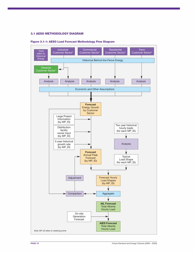
3.1 AESO METHODOLOGY DIAGRAM
Figure 3.1-1: AESO Load Forecast Methodology Flow Diagram
Note: MP_ID refers to metering points
Industrial Customer Sector*
* Note:refers toHistoricalEnergy
Commercial Customer Sector*
Residential Customer Sector*
Farm Customer Sector*
Historical Behind-the-Fence Energy
Oilsands Customer Sector*
Analysis Analysis Analysis Analysis Analysis
Economic and Other Assumptions
ForecastAnnual PeakForecast(by MP_ID)
Analysis
Two year historicalhourly loads
(for each MP_ID)
Large ProjectInformation(by MP_ID)
Distributionfacility
owner input(by MP_ID)
5-year historical growth rate(by MP_ID)
AIES ForecastTotal AlbertaHourly Load
AIL ForecastTotal AlbertaHourly Load
On-siteGenerationForecast
Aggregate
Forecast HourlyLoad Shapes(by MP_ID)
Typical Load Shape
(for each MP_ID)
ForecastEnergy Growthby Customer
Sector
Adjustment
Comparison
Future Demand and Energy Outlook (2009 – 2029) PAGE 11
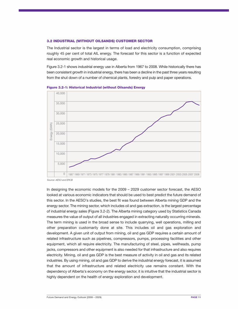
3.2 INDUSTRIAL (WITHOUT OILSANDS) CUSTOMER SECTOR
The Industrial sector is the largest in terms of load and electricity consumption, comprising
roughly 45 per cent of total AIL energy. The forecast for this sector is a function of expected
real economic growth and historical usage.
Figure 3.2-1 shows industrial energy use in Alberta from 1967 to 2008. While historically there has
been consistent growth in industrial energy, there has been a decline in the past three years resulting
from the shut down of a number of chemical plants, forestry and pulp and paper operations.
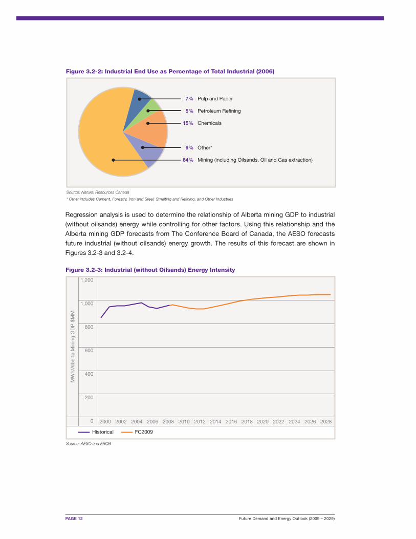
In designing the economic models for the 2009 – 2029 customer sector forecast, the AESO
looked at various economic indicators that should be used to best predict the future demand of
this sector. In the AESO’s studies, the best fit was found between Alberta mining GDP and the
energy sector. The mining sector, which includes oil and gas extraction, is the largest percentage
of industrial energy sales (Figure 3.2-2). The Alberta mining category used by Statistics Canada
measures the value of output of all industries engaged in extracting naturally occurring minerals.
The term mining is used in the broad sense to include quarrying, well operations, milling and
other preparation customarily done at site. This includes oil and gas exploration and
development. A given unit of output from mining, oil and gas GDP requires a certain amount of
related infrastructure such as pipelines, compressors, pumps, processing facilities and other
equipment, which all require electricity. The manufacturing of steel, pipes, wellheads, pump
jacks, compressors and other equipment is also needed for that infrastructure and also requires
electricity. Mining, oil and gas GDP is the best measure of activity in oil and gas and its related
industries. By using mining, oil and gas GDP to derive the industrial energy forecast, it is assumed
that the amount of infrastructure and related electricity use remains constant. With the
dependency of Alberta’s economy on the energy sector, it is intuitive that the industrial sector is
highly dependent on the health of energy exploration and development.
40,000
35,000
30,000
25,000
20,000
15,000
10,000
5,000
0
Source: AESO and ERCB
1967 1969 1971 1973 1975 1977 1979 1981 1983 1985 1987 1989 1991 1993 1995 1997 1999 2001 2003 2005 2007 2008
Ene
rgy
(GW
h)
Figure 3.2-1: Historical Industrial (without Oilsands) Energy
PAGE 12 Future Demand and Energy Outlook (2009 – 2029)
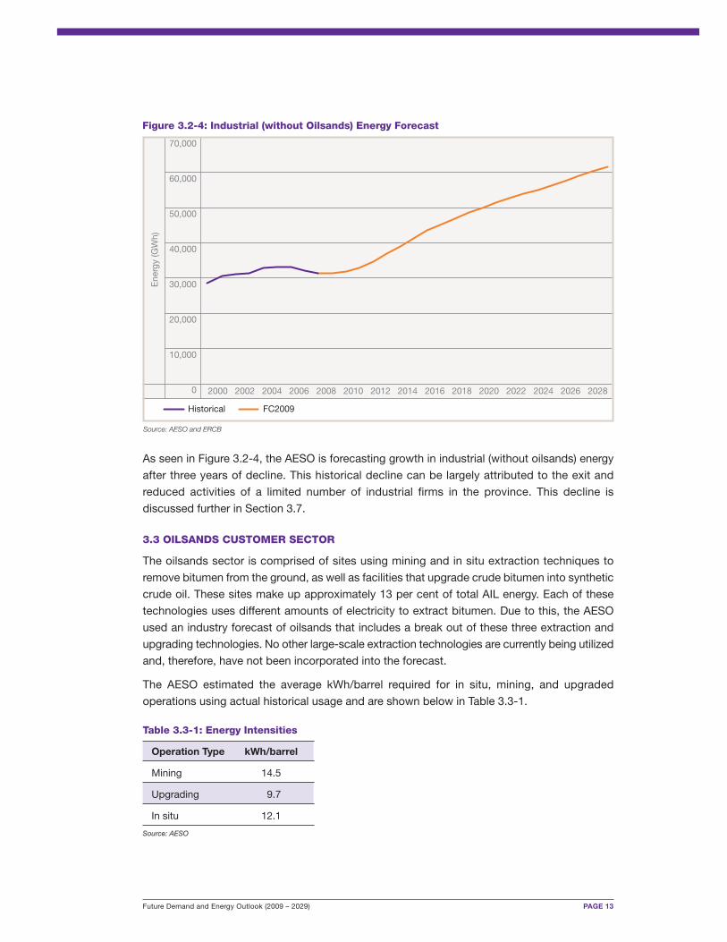
Regression analysis is used to determine the relationship of Alberta mining GDP to industrial
(without oilsands) energy while controlling for other factors. Using this relationship and the
Alberta mining GDP forecasts from The Conference Board of Canada, the AESO forecasts
future industrial (without oilsands) energy growth. The results of this forecast are shown in
Figures 3.2-3 and 3.2-4.
Figure 3.2-2: Industrial End Use as Percentage of Total Industrial (2006)
7% Pulp and Paper
5% Petroleum Refining
15% Chemicals
9% Other*
64% Mining (including Oilsands, Oil and Gas extraction)
Source: Natural Resources Canada
* Other includes Cement, Forestry, Iron and Steel, Smelting and Refining, and Other Industries
1,200
1,000
800
600
400
200
0
Source: AESO and ERCB
2000 2002 2004 2006 2008 2010 2012 2014 2016 2018 2020 2022 2024 2026 2028
FC2009
MW
h/A
lber
ta M
inin
g G
DP
$M
M
Figure 3.2-3: Industrial (without Oilsands) Energy Intensity
Historical
Future Demand and Energy Outlook (2009 – 2029) PAGE 13
70,000
60,000
50,000
40,000
30,000
20,000
10,000
0
Source: AESO and ERCB
2000 2002 2004 2006 2008 2010 2012 2014 2016 2018 2020 2022 2024 2026 2028
FC2009
Ene
rgy
(GW
h)
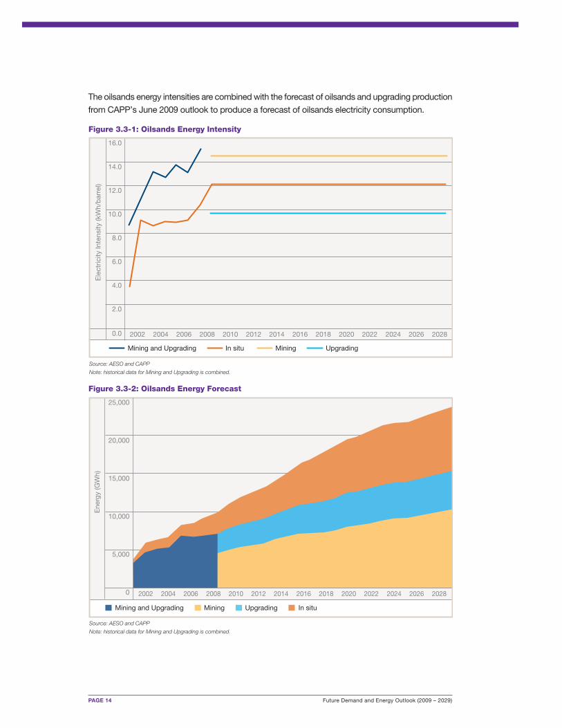
Figure 3.2-4: Industrial (without Oilsands) Energy Forecast
Historical
As seen in Figure 3.2-4, the AESO is forecasting growth in industrial (without oilsands) energy
after three years of decline. This historical decline can be largely attributed to the exit and
reduced activities of a limited number of industrial firms in the province. This decline is
discussed further in Section 3.7.
3.3 OILSANDS CUSTOMER SECTOR
The oilsands sector is comprised of sites using mining and in situ extraction techniques to
remove bitumen from the ground, as well as facilities that upgrade crude bitumen into synthetic
crude oil. These sites make up approximately 13 per cent of total AIL energy. Each of these
technologies uses different amounts of electricity to extract bitumen. Due to this, the AESO
used an industry forecast of oilsands that includes a break out of these three extraction and
upgrading technologies. No other large-scale extraction technologies are currently being utilized
and, therefore, have not been incorporated into the forecast.
The AESO estimated the average kWh/barrel required for in situ, mining, and upgraded
operations using actual historical usage and are shown below in Table 3.3-1.
Table 3.3-1: Energy Intensities
Operation Type kWh/barrel
Mining 14.5
Upgrading 9.7
In situ 12.1
Source: AESO
PAGE 14 Future Demand and Energy Outlook (2009 – 2029)
The oilsands energy intensities are combined with the forecast of oilsands and upgrading production
from CAPP’s June 2009 outlook to produce a forecast of oilsands electricity consumption.
16.0
14.0
12.0
10.0
8.0
6.0
4.0
2.0
0.0
Source: AESO and CAPP
Note: historical data for Mining and Upgrading is combined.
Mining and Upgrading
Ele
ctric
ity In
tens
ity (k
Wh/
bar
rel)
Figure 3.3-1: Oilsands Energy Intensity
In situ Mining Upgrading
2002 2004 2006 2008 2010 2012 2014 2016 2018 2020 2022 2024 2026 2028
25,000
20,000
15,000
10,000
5,000
0
Source: AESO and CAPP
Note: historical data for Mining and Upgrading is combined.
2002 2004 2006 2008 2010 2012 2014 2016 2018 2020 2022 2024 2026 2028
Figure 3.3-2: Oilsands Energy Forecast
Ene
rgy
(GW
h)
Mining and Upgrading In situMining Upgrading
Future Demand and Energy Outlook (2009 – 2029) PAGE 15
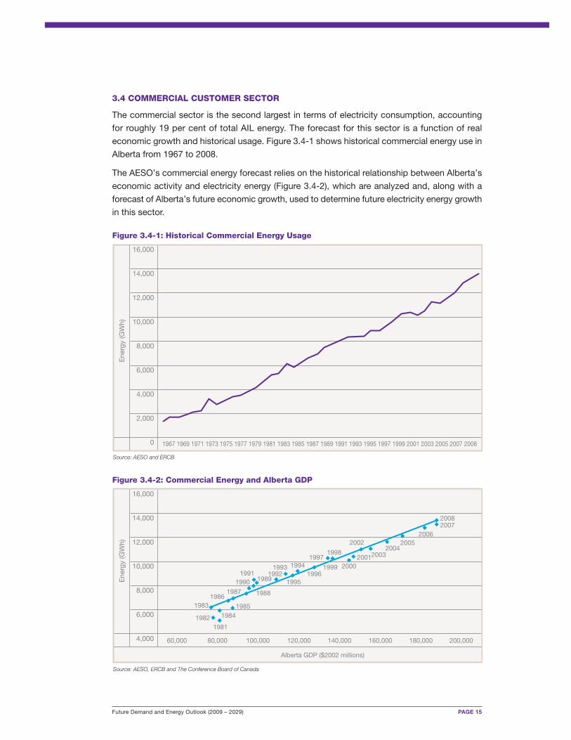
3.4 COMMERCIAL CUSTOMER SECTOR
The commercial sector is the second largest in terms of electricity consumption, accounting
for roughly 19 per cent of total AIL energy. The forecast for this sector is a function of real
economic growth and historical usage. Figure 3.4-1 shows historical commercial energy use in
Alberta from 1967 to 2008.
The AESO’s commercial energy forecast relies on the historical relationship between Alberta’s
economic activity and electricity energy (Figure 3.4-2), which are analyzed and, along with a
forecast of Alberta’s future economic growth, used to determine future electricity energy growth
in this sector.
16,000
14,000
12,000
10,000
8,000
6,000
4,000
2,000
0
Source: AESO and ERCB
1967 1969 1971 1973 1975 1977 1979 1981 1983 1985 1987 1989 1991 1993 1995 1997 1999 2001 2003 2005 2007 2008
Figure 3.4-1: Historical Commercial Energy Usage
Ene
rgy
(GW
h)
16,000
14,000
12,000
10,000
8,000
6,000
4,000
20082007
20062005
20042003
2002
20012000
1995
19941996
199319921991
1990
1986
1984
1983
1987 1988
1989
1985
19811982
19971998
1999
Source: AESO, ERCB and The Conference Board of Canada
80,00060,000
Alberta GDP ($2002 millions)
200,000100,000 120,000 140,000 160,000 180,000
Figure 3.4-2: Commercial Energy and Alberta GDP
Ene
rgy
(GW
h)
PAGE 16 Future Demand and Energy Outlook (2009 – 2029)
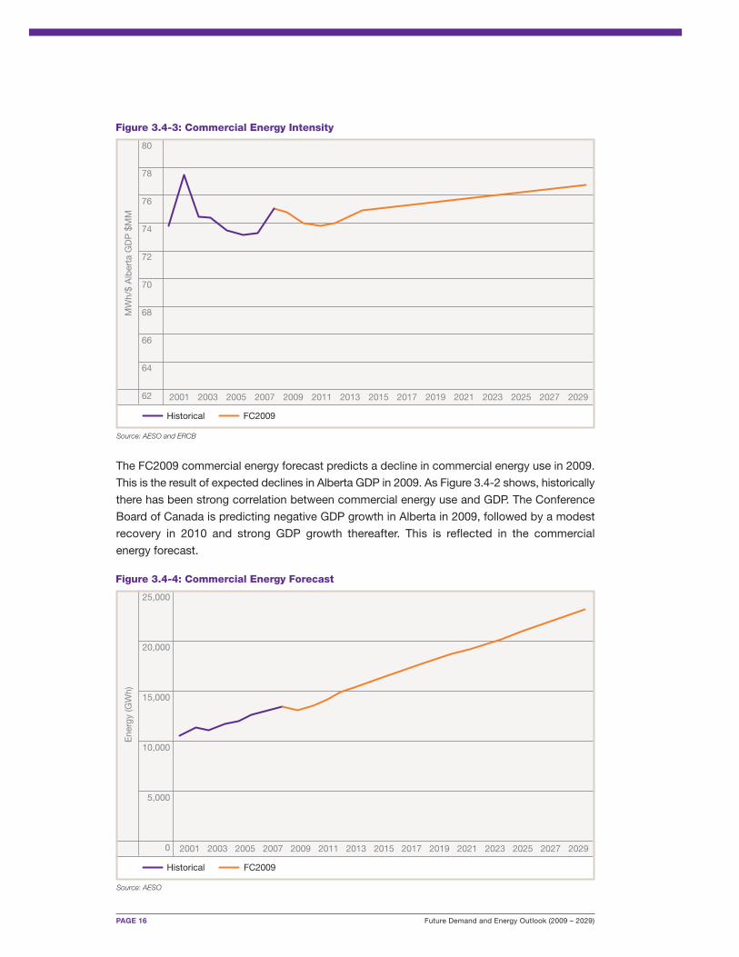
The FC2009 commercial energy forecast predicts a decline in commercial energy use in 2009.
This is the result of expected declines in Alberta GDP in 2009. As Figure 3.4-2 shows, historically
there has been strong correlation between commercial energy use and GDP. The Conference
Board of Canada is predicting negative GDP growth in Alberta in 2009, followed by a modest
recovery in 2010 and strong GDP growth thereafter. This is reflected in the commercial
energy forecast.
80
78
76
74
72
70
68
66
64
62
Source: AESO and ERCB
FC2009
MW
h/$
Alb
erta
GD
P $
MM
Figure 3.4-3: Commercial Energy Intensity
Historical
2001 2003 2005 2007 2009 2011 2013 2015 2017 2019 2021 2023 2025 2027 2029
25,000
20,000
15,000
10,000
5,000
0
Source: AESO
FC2009
Ene
rgy
(GW
h)
Figure 3.4-4: Commercial Energy Forecast
Historical
2001 2003 2005 2007 2009 2011 2013 2015 2017 2019 2021 2023 2025 2027 2029
Future Demand and Energy Outlook (2009 – 2029) PAGE 17
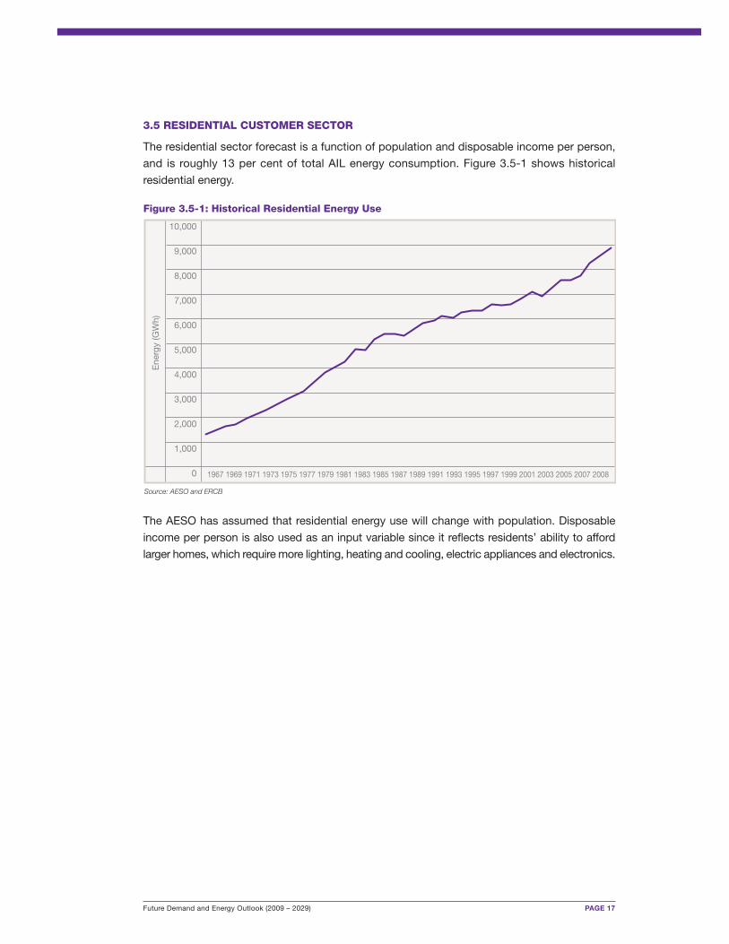
3.5 RESIDENTIAL CUSTOMER SECTOR
The residential sector forecast is a function of population and disposable income per person,
and is roughly 13 per cent of total AIL energy consumption. Figure 3.5-1 shows historical
residential energy.
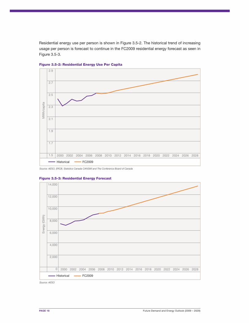
The AESO has assumed that residential energy use will change with population. Disposable
income per person is also used as an input variable since it reflects residents’ ability to afford
larger homes, which require more lighting, heating and cooling, electric appliances and electronics.
10,000
9,000
8,000
7,000
6,000
5,000
4,000
3,000
2,000
1,000
0
Source: AESO and ERCB
1967 1969 1971 1973 1975 1977 1979 1981 1983 1985 1987 1989 1991 1993 1995 1997 1999 2001 2003 2005 2007 2008
Figure 3.5-1: Historical Residential Energy Use
Ene
rgy
(GW
h)
PAGE 18 Future Demand and Energy Outlook (2009 – 2029)
2.9
2.7
2.5
2.3
2.1
1.9
1.7
1.5
Source: AESO, ERCB, Statistics Canada CANSIM and The Conference Board of Canada
MW
h/ca
pita
Figure 3.5-2: Residential Energy Use Per Capita
2002 20042000 2006 2008 2010 2012 2014 2016 2018 2020 2022 2024 2026 2028
FC2009Historical
14,000
12,000
10,000
8,000
6,000
4,000
2,000
0
Source: AESO
Ene
rgy
(GW
h)
Figure 3.5-3: Residential Energy Forecast
2002 20042000 2006 2008 2010 2012 2014 2016 2018 2020 2022 2024 2026 2028
FC2009Historical
Residential energy use per person is shown in Figure 3.5-2. The historical trend of increasing
usage per person is forecast to continue in the FC2009 residential energy forecast as seen in
Figure 3.5-3.
Future Demand and Energy Outlook (2009 – 2029) PAGE 19
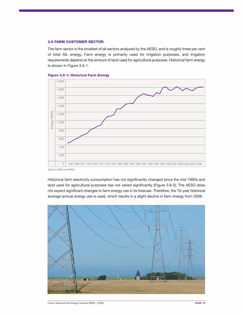
3.6 FARM CUSTOMER SECTOR
The farm sector is the smallest of all sectors analyzed by the AESO, and is roughly three per cent
of total AIL energy. Farm energy is primarily used for irrigation purposes, and irrigation
requirements depend on the amount of land used for agricultural purposes. Historical farm energy
is shown in Figure 3.6-1.
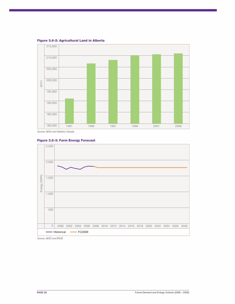
Historical farm electricity consumption has not significantly changed since the mid 1990s and
land used for agricultural purposes has not varied significantly (Figure 3.6-2). The AESO does
not expect significant changes to farm energy use in its forecast. Therefore, the 10-year historical
average annual energy use is used, which results in a slight decline in farm energy from 2008.
2,000
1,800
1,600
1,400
1,200
1,000
800
600
400
200
0
Source: AESO and ERCB
1967 1969 1971 1973 1975 1977 1979 1981 1983 1985 1987 1989 1991 1993 1995 1997 1999 2001 2003 2005 2007 2008
Figure 3.6-1: Historical Farm Energy
Ene
rgy
(GW
h)
PAGE 20 Future Demand and Energy Outlook (2009 – 2029)
215,000
210,000
205,000
200,000
195,000
190,000
185,000
180,000
Source: AESO and Statistics Canada
1981 1986 1991 1996 2001 2006
Figure 3.6-2: Agricultural Land in Alberta(k
m2)
2,500
2,000
1,500
1,000
500
0
Source: AESO and ERCB
Ene
rgy
(GW
h)
Figure 3.6-3: Farm Energy Forecast
2002 20042000 2006 2008 2010 2012 2014 2016 2018 2020 2022 2024 2026 2028
FC2009Historical
Future Demand and Energy Outlook (2009 – 2029) PAGE 21
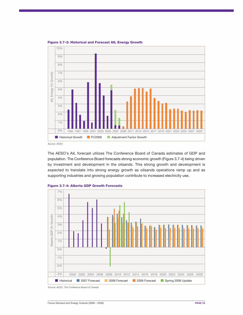
3.7 HISTORICAL GROWTH AND DECREASE IN 10 INDUSTRIAL SITES
AIL energy use over the past five years grew at an annualized rate of 1.5 per cent. However,
the AESO is forecasting energy growth to average 4.4 per cent annually over the period from
2009 to 2014 and 3.2 per cent over the period from 2009 to 2029. This difference in growth rates
can be explained through a combination of factors.
Over the past five years, Alberta has been characterized by strong economic growth as a result
of a booming oil and gas industry caused by high commodity prices. However, as the oil and
gas industry boomed, other industries in the province did not. Specifically, the pulp and paper,
forestry, and chemical industries suffered due to higher costs and lower demand. All three
industries faced higher labour and materials costs. The rapidly growing oil and gas industry
created low unemployment in Alberta, causing upward pressure on wages, especially for skilled
workers. Demand by the oil and gas industry for materials such as steel and cement also
increased, resulting in higher costs for all industries.
While costs rose, the pulp and paper, forestry, and chemical industries also faced decreased
demand for their products. Demand for pulp and paper declined as a result of the decline of
newsprint. Demand for Alberta forestry products has also declined since the U.S. housing
market peaked in early 2006 and subsequently decreased. Demand for sodium chlorate, which
is used to bleach pulp and paper, has also declined.
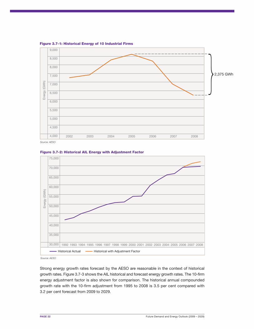
Figure 3.7-1 shows the combined electricity consumption of 10 industrial firms which operate
or operated in Alberta in the forestry, pulp and paper, and chemical industries. These firms have
either shut down or ramped down operations since 2005, resulting in decreased energy use.
Analysis indicates they had decreased energy use by 2,375 GWh per year in 2008 compared
to 2005 levels. This adjustment factor of 2,375 GWh could have increased AIL energy in 2008
by 3.4 per cent (see Table 6.1-2). Assuming this decrease of 2,375 GWh had not occurred
between 2005 and 2008 by these 10 industrial firms, AIL energy would have had a five-year
average annual growth rate of 2.9 per cent instead of 2.2 per cent.
It is not possible to predict how or when a given firm may choose to shut down or ramp down
operations. However, a recent rebound in pulp and paper prices and a recovering U.S. housing
market, combined with an expected overall economic recovery, suggest it is less likely
companies will shut down or ramp down operations in the foreseeable future. In addition, the
small portion of pulp and paper, forestry, and chemical companies as a fraction of industrial
energy use suggests there is minimal potential additional loss from further shut down or ramp
down of these industries.
PAGE 22 Future Demand and Energy Outlook (2009 – 2029)
Strong energy growth rates forecast by the AESO are reasonable in the context of historical
growth rates. Figure 3.7-3 shows the AIL historical and forecast energy growth rates. The 10-firm
energy adjustment factor is also shown for comparison. The historical annual compounded
growth rate with the 10-firm adjustment from 1995 to 2008 is 3.5 per cent compared with
3.2 per cent forecast from 2009 to 2029.
9,000
8,500
8,000
7,500
7,000
6,500
6,000
5,500
5,000
4,500
4,000
2,375 GWh
Source: AESO
Ene
rgy
(GW
h)Figure 3.7-1: Historical Energy of 10 Industrial Firms
2003 20042002 2005 2006 2007 2008
75,000
70,000
65,000
60,000
55,000
50,000
45,000
40,000
35,000
30,000
Source: AESO
Ene
rgy
(GW
h)
Figure 3.7-2: Historical AIL Energy with Adjustment Factor
1993 19941992 1995 1996 1997 1998 1999 2001 20022000 2003 2004 2005 2006 2007 2008
Historical Actual Historical with Adjustment Factor
Future Demand and Energy Outlook (2009 – 2029) PAGE 23
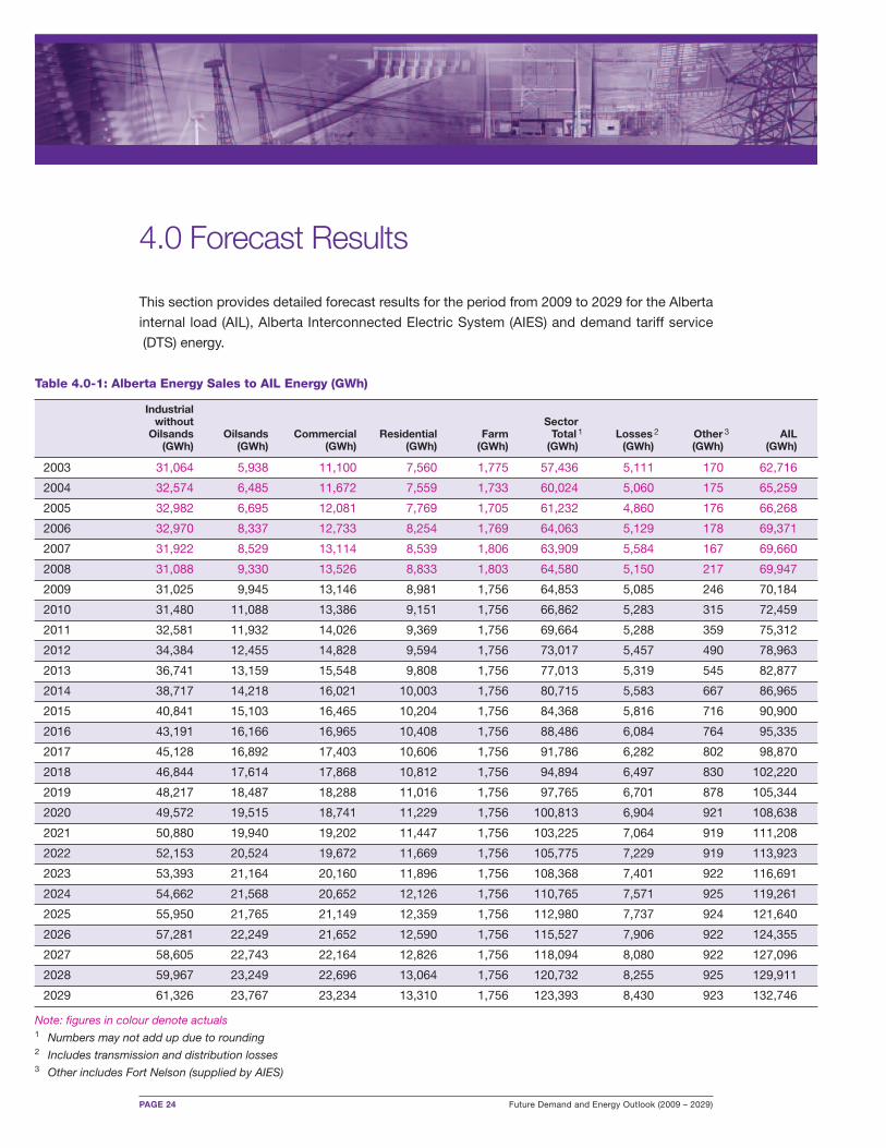
The AESO’s AIL forecast utilizes The Conference Board of Canada estimates of GDP and
population. The Conference Board forecasts strong economic growth (Figure 3.7-4) being driven
by investment and development in the oilsands. This strong growth and development is
expected to translate into strong energy growth as oilsands operations ramp up and as
supporting industries and growing population contribute to increased electricity use.
10%
9%
8%
7%
6%
5%
4%
3%
2%
1%
0%
Source: AESO
AIL
Ene
rgy
(% G
row
th)
Figure 3.7-3: Historical and Forecast AIL Energy Growth
1997 19991995 2001 2003 2005 2007 2009 2013 20152011 2017 2019 2021 2023 2025 2027 2029
FC2009 Adjustment Factor GrowthHistorical Growth
7%
6%
5%
4%
3%
2%
1%
0%
-1%
-2%
-3%
Source: AESO, The Conference Board of Canada
Alb
erta
GD
P (%
Gro
wth
)
Figure 3.7-4: Alberta GDP Growth Forecasts
2000 2002 2004 2006 2008 2012 20142010 2016 2018 2020 2022 2024 2026 2028
2007 Forecast 2008 Forecast 2009 Forecast Spring 2009 UpdateHistorical
PAGE 24 Future Demand and Energy Outlook (2009 – 2029)
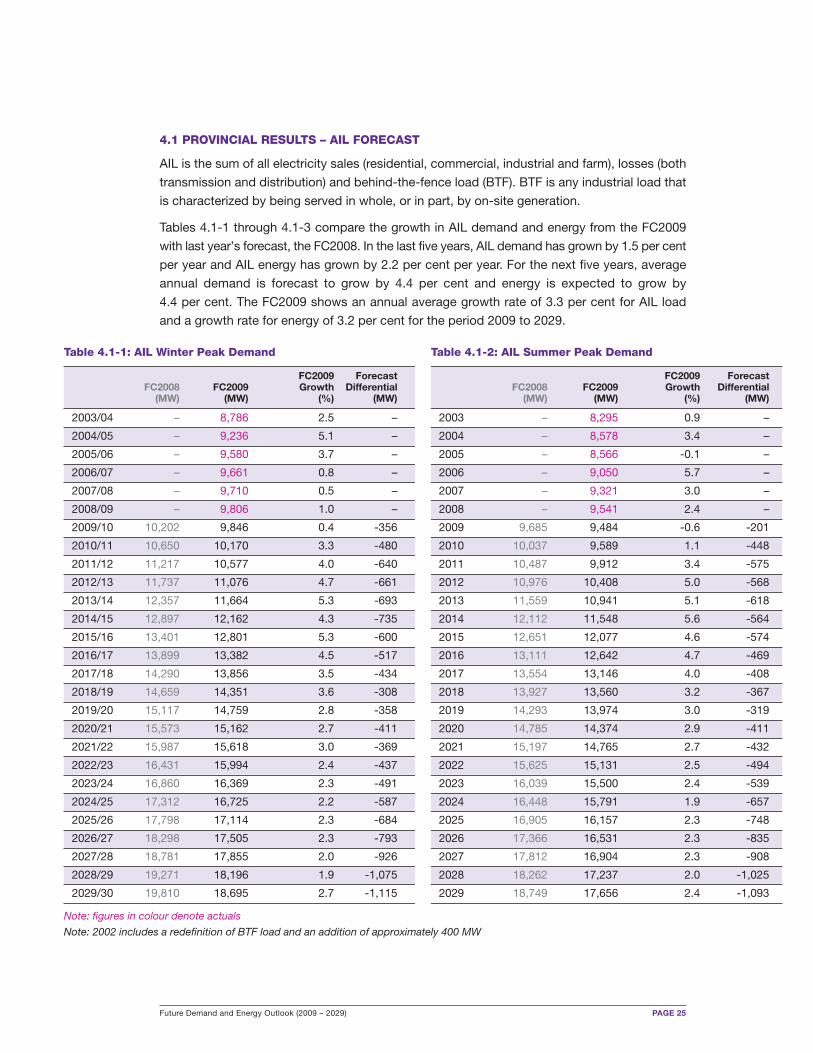
4.0 Forecast Results
This section provides detailed forecast results for the period from 2009 to 2029 for the Alberta
internal load (AIL), Alberta Interconnected Electric System (AIES) and demand tariff service
(DTS) energy.
Table 4.0-1: Alberta Energy Sales to AIL Energy (GWh)
Industrial without SectorOilsands Oilsands Commercial Residential Farm Total 1 Losses 2 Other 3 AIL(GWh) (GWh) (GWh) (GWh) (GWh) (GWh) (GWh) (GWh) (GWh)
2003 31,064 5,938 11,100 7,560 1,775 57,436 5,111 170 62,716
2004 32,574 6,485 11,672 7,559 1,733 60,024 5,060 175 65,259
2005 32,982 6,695 12,081 7,769 1,705 61,232 4,860 176 66,268
2006 32,970 8,337 12,733 8,254 1,769 64,063 5,129 178 69,371
2007 31,922 8,529 13,114 8,539 1,806 63,909 5,584 167 69,660
2008 31,088 9,330 13,526 8,833 1,803 64,580 5,150 217 69,947
2009 31,025 9,945 13,146 8,981 1,756 64,853 5,085 246 70,184
2010 31,480 11,088 13,386 9,151 1,756 66,862 5,283 315 72,459
2011 32,581 11,932 14,026 9,369 1,756 69,664 5,288 359 75,312
2012 34,384 12,455 14,828 9,594 1,756 73,017 5,457 490 78,963
2013 36,741 13,159 15,548 9,808 1,756 77,013 5,319 545 82,877
2014 38,717 14,218 16,021 10,003 1,756 80,715 5,583 667 86,965
2015 40,841 15,103 16,465 10,204 1,756 84,368 5,816 716 90,900
2016 43,191 16,166 16,965 10,408 1,756 88,486 6,084 764 95,335
2017 45,128 16,892 17,403 10,606 1,756 91,786 6,282 802 98,870
2018 46,844 17,614 17,868 10,812 1,756 94,894 6,497 830 102,220
2019 48,217 18,487 18,288 11,016 1,756 97,765 6,701 878 105,344
2020 49,572 19,515 18,741 11,229 1,756 100,813 6,904 921 108,638
2021 50,880 19,940 19,202 11,447 1,756 103,225 7,064 919 111,208
2022 52,153 20,524 19,672 11,669 1,756 105,775 7,229 919 113,923
2023 53,393 21,164 20,160 11,896 1,756 108,368 7,401 922 116,691
2024 54,662 21,568 20,652 12,126 1,756 110,765 7,571 925 119,261
2025 55,950 21,765 21,149 12,359 1,756 112,980 7,737 924 121,640
2026 57,281 22,249 21,652 12,590 1,756 115,527 7,906 922 124,355
2027 58,605 22,743 22,164 12,826 1,756 118,094 8,080 922 127,096
2028 59,967 23,249 22,696 13,064 1,756 120,732 8,255 925 129,911
2029 61,326 23,767 23,234 13,310 1,756 123,393 8,430 923 132,746
Note: figures in colour denote actuals1 Numbers may not add up due to rounding2 Includes transmission and distribution losses 3 Other includes Fort Nelson (supplied by AIES)
Future Demand and Energy Outlook (2009 – 2029) PAGE 25
4.1 PROVINCIAL RESULTS – AIL FORECAST
AIL is the sum of all electricity sales (residential, commercial, industrial and farm), losses (both
transmission and distribution) and behind-the-fence load (BTF). BTF is any industrial load that
is characterized by being served in whole, or in part, by on-site generation.
Tables 4.1-1 through 4.1-3 compare the growth in AIL demand and energy from the FC2009
with last year’s forecast, the FC2008. In the last five years, AIL demand has grown by 1.5 per cent
per year and AIL energy has grown by 2.2 per cent per year. For the next five years, average
annual demand is forecast to grow by 4.4 per cent and energy is expected to grow by
4.4 per cent. The FC2009 shows an annual average growth rate of 3.3 per cent for AIL load
and a growth rate for energy of 3.2 per cent for the period 2009 to 2029.
Table 4.1-1: AIL Winter Peak Demand Table 4.1-2: AIL Summer Peak Demand
FC2009 Forecast FC2009 ForecastFC2008 FC2009 Growth Differential FC2008 FC2009 Growth Differential(MW) (MW) (%) (MW) (MW) (MW) (%) (MW)
2003/04 – 8,786 2.5 – 2003 – 8,295 0.9 –
2004/05 – 9,236 5.1 – 2004 – 8,578 3.4 –
2005/06 – 9,580 3.7 – 2005 – 8,566 -0.1 –
2006/07 – 9,661 0.8 – 2006 – 9,050 5.7 –
2007/08 – 9,710 0.5 – 2007 – 9,321 3.0 –
2008/09 – 9,806 1.0 – 2008 – 9,541 2.4 –
2009/10 10,202 9,846 0.4 -356 2009 9,685 9,484 -0.6 -201
2010/11 10,650 10,170 3.3 -480 2010 10,037 9,589 1.1 -448
2011/12 11,217 10,577 4.0 -640 2011 10,487 9,912 3.4 -575
2012/13 11,737 11,076 4.7 -661 2012 10,976 10,408 5.0 -568
2013/14 12,357 11,664 5.3 -693 2013 11,559 10,941 5.1 -618
2014/15 12,897 12,162 4.3 -735 2014 12,112 11,548 5.6 -564
2015/16 13,401 12,801 5.3 -600 2015 12,651 12,077 4.6 -574
2016/17 13,899 13,382 4.5 -517 2016 13,111 12,642 4.7 -469
2017/18 14,290 13,856 3.5 -434 2017 13,554 13,146 4.0 -408
2018/19 14,659 14,351 3.6 -308 2018 13,927 13,560 3.2 -367
2019/20 15,117 14,759 2.8 -358 2019 14,293 13,974 3.0 -319
2020/21 15,573 15,162 2.7 -411 2020 14,785 14,374 2.9 -411
2021/22 15,987 15,618 3.0 -369 2021 15,197 14,765 2.7 -432
2022/23 16,431 15,994 2.4 -437 2022 15,625 15,131 2.5 -494
2023/24 16,860 16,369 2.3 -491 2023 16,039 15,500 2.4 -539
2024/25 17,312 16,725 2.2 -587 2024 16,448 15,791 1.9 -657
2025/26 17,798 17,114 2.3 -684 2025 16,905 16,157 2.3 -748
2026/27 18,298 17,505 2.3 -793 2026 17,366 16,531 2.3 -835
2027/28 18,781 17,855 2.0 -926 2027 17,812 16,904 2.3 -908
2028/29 19,271 18,196 1.9 -1,075 2028 18,262 17,237 2.0 -1,025
2029/30 19,810 18,695 2.7 -1,115 2029 18,749 17,656 2.4 -1,093
Note: figures in colour denote actuals
Note: 2002 includes a redefinition of BTF load and an addition of approximately 400 MW
PAGE 26 Future Demand and Energy Outlook (2009 – 2029)
Table 4.1-3: AIL Annual Energy
ForecastFC2008 FC2009 FC2009 Differential Load(GWh) (GWh) Growth (%) (GWh) Factor (%)
2003 – 62,716 5.5 – 79.8
2004 – 65,259 4.1 – 82.9
2005 – 66,268 1.5 – 81.9
2006 – 69,371 4.7 – 82.7
2007 – 69,660 0.4 – 82.3
2008 – 69,947 0.4 – 82.2
2009 73,062 70,184 0.3 -2,878 81.7
2010 75,727 72,459 3.2 -3,268 84.0
2011 79,146 75,312 3.9 -3,834 84.5
2012 83,485 78,963 4.8 -4,522 85.0
2013 87,678 82,877 5.0 -4,801 85.4
2014 92,106 86,965 4.9 -5,141 85.1
2015 96,448 90,900 4.5 -5,548 85.3
2016 100,487 95,335 4.9 -5,152 84.8
2017 103,841 98,870 3.7 -4,971 84.3
2018 106,775 102,220 3.4 -4,555 84.2
2019 109,562 105,344 3.1 -4,218 83.8
2020 113,652 108,638 3.1 -5,014 83.8
2021 116,626 111,208 2.4 -5,418 83.7
2022 119,804 113,923 2.4 -5,881 83.3
2023 123,028 116,691 2.4 -6,337 83.3
2024 126,376 119,261 2.2 -7,115 82.9
2025 129,601 121,640 2.0 -7,961 83.0
2026 133,049 124,355 2.2 -8,694 82.9
2027 136,584 127,096 2.2 -9,488 82.9
2028 140,265 129,911 2.2 -10,354 82.8
2029 143,760 132,746 2.2 -11,014 83.3
Note: figures in colour denote actuals
Note: 2002 includes a redefinition of BTF load and an addition of approximately 400 MW
Future Demand and Energy Outlook (2009 – 2029) PAGE 27
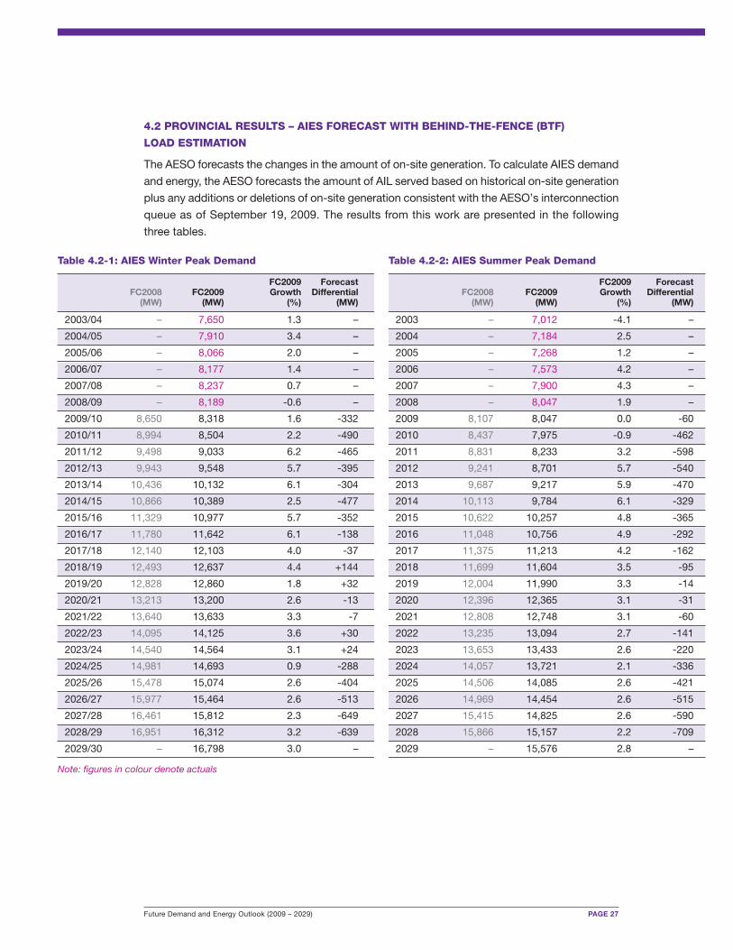
4.2 PROVINCIAL RESULTS – AIES FORECAST WITH BEHIND-THE-FENCE (BTF)
LOAD ESTIMATION
The AESO forecasts the changes in the amount of on-site generation. To calculate AIES demand
and energy, the AESO forecasts the amount of AIL served based on historical on-site generation
plus any additions or deletions of on-site generation consistent with the AESO’s interconnection
queue as of September 19, 2009. The results from this work are presented in the following
three tables.
Table 4.2-1: AIES Winter Peak Demand Table 4.2-2: AIES Summer Peak Demand
FC2009 Forecast FC2009 ForecastFC2008 FC2009 Growth Differential FC2008 FC2009 Growth Differential(MW) (MW) (%) (MW) (MW) (MW) (%) (MW)
2003/04 – 7,650 1.3 – 2003 – 7,012 -4.1 –
2004/05 – 7,910 3.4 – 2004 – 7,184 2.5 –
2005/06 – 8,066 2.0 – 2005 – 7,268 1.2 –
2006/07 – 8,177 1.4 – 2006 – 7,573 4.2 –
2007/08 – 8,237 0.7 – 2007 – 7,900 4.3 –
2008/09 – 8,189 -0.6 – 2008 – 8,047 1.9 –
2009/10 8,650 8,318 1.6 -332 2009 8,107 8,047 0.0 -60
2010/11 8,994 8,504 2.2 -490 2010 8,437 7,975 -0.9 -462
2011/12 9,498 9,033 6.2 -465 2011 8,831 8,233 3.2 -598
2012/13 9,943 9,548 5.7 -395 2012 9,241 8,701 5.7 -540
2013/14 10,436 10,132 6.1 -304 2013 9,687 9,217 5.9 -470
2014/15 10,866 10,389 2.5 -477 2014 10,113 9,784 6.1 -329
2015/16 11,329 10,977 5.7 -352 2015 10,622 10,257 4.8 -365
2016/17 11,780 11,642 6.1 -138 2016 11,048 10,756 4.9 -292
2017/18 12,140 12,103 4.0 -37 2017 11,375 11,213 4.2 -162
2018/19 12,493 12,637 4.4 +144 2018 11,699 11,604 3.5 -95
2019/20 12,828 12,860 1.8 +32 2019 12,004 11,990 3.3 -14
2020/21 13,213 13,200 2.6 -13 2020 12,396 12,365 3.1 -31
2021/22 13,640 13,633 3.3 -7 2021 12,808 12,748 3.1 -60
2022/23 14,095 14,125 3.6 +30 2022 13,235 13,094 2.7 -141
2023/24 14,540 14,564 3.1 +24 2023 13,653 13,433 2.6 -220
2024/25 14,981 14,693 0.9 -288 2024 14,057 13,721 2.1 -336
2025/26 15,478 15,074 2.6 -404 2025 14,506 14,085 2.6 -421
2026/27 15,977 15,464 2.6 -513 2026 14,969 14,454 2.6 -515
2027/28 16,461 15,812 2.3 -649 2027 15,415 14,825 2.6 -590
2028/29 16,951 16,312 3.2 -639 2028 15,866 15,157 2.2 -709
2029/30 – 16,798 3.0 – 2029 – 15,576 2.8 –
Note: figures in colour denote actuals
PAGE 28 Future Demand and Energy Outlook (2009 – 2029)
Table 4.2-3: AIES Annual Energy
FC2009 Forecast FC2008 FC2009 Growth Differential Load(GWh) (GWh) (%) (GWh) Factor (%)
2003 – 53,169 -0.9 – 79.3
2004 – 54,669 2.8 – 78.7
2005 – 55,697 1.9 – 78.8
2006 – 57,433 3.1 – 80.2
2007 – 57,701 0.5 – 80.0
2008 – 57,934 0.4 – 80.5
2009 60,105 58,115 0.3 -1,990 79.8
2010 62,364 59,430 2.3 -2,934 79.8
2011 65,368 61,716 3.8 -3,652 78.0
2012 69,139 65,132 5.5 -4,007 77.7
2013 72,648 68,792 5.6 -3,856 77.5
2014 76,020 72,512 5.4 -3,508 79.7
2015 79,833 75,984 4.8 -3,849 79.0
2016 83,521 79,927 5.2 -3,594 78.2
2017 86,293 83,163 4.0 -3,130 78.4
2018 88,531 86,334 3.8 -2,197 78.0
2019 90,809 89,232 3.4 -1,577 79.2
2020 93,794 92,269 3.4 -1,525 79.6
2021 96,722 94,812 2.8 -1,910 79.4
2022 99,830 97,381 2.7 -2,449 78.7
2023 103,009 99,887 2.6 -3,122 78.3
2024 106,226 102,329 2.4 3,897 79.3
2025 109,462 104,716 2.3 -4,746 79.3
2026 112,916 107,368 2.5 -5,548 79.3
2027 116,447 110,090 2.5 -6,357 79.5
2028 120,051 112,853 2.5 -7,198 78.8
2029 – 115,715 2.5 – 78.6
Note: figures in colour denote actuals
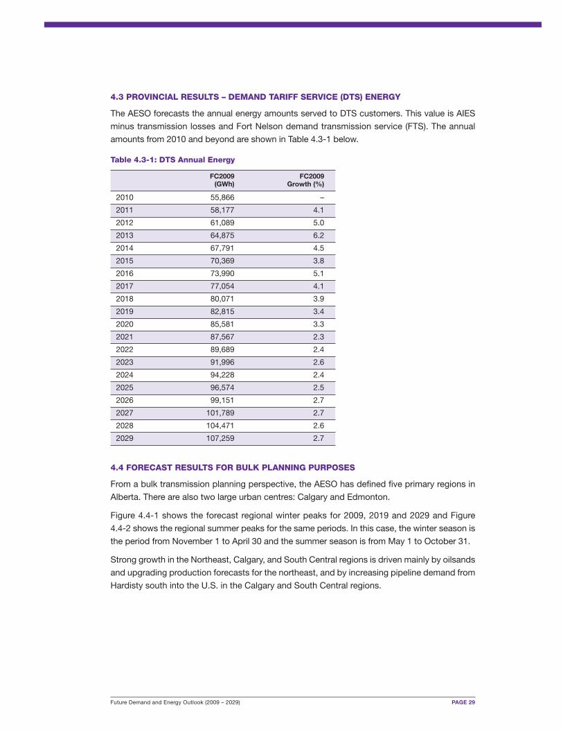
Future Demand and Energy Outlook (2009 – 2029) PAGE 29
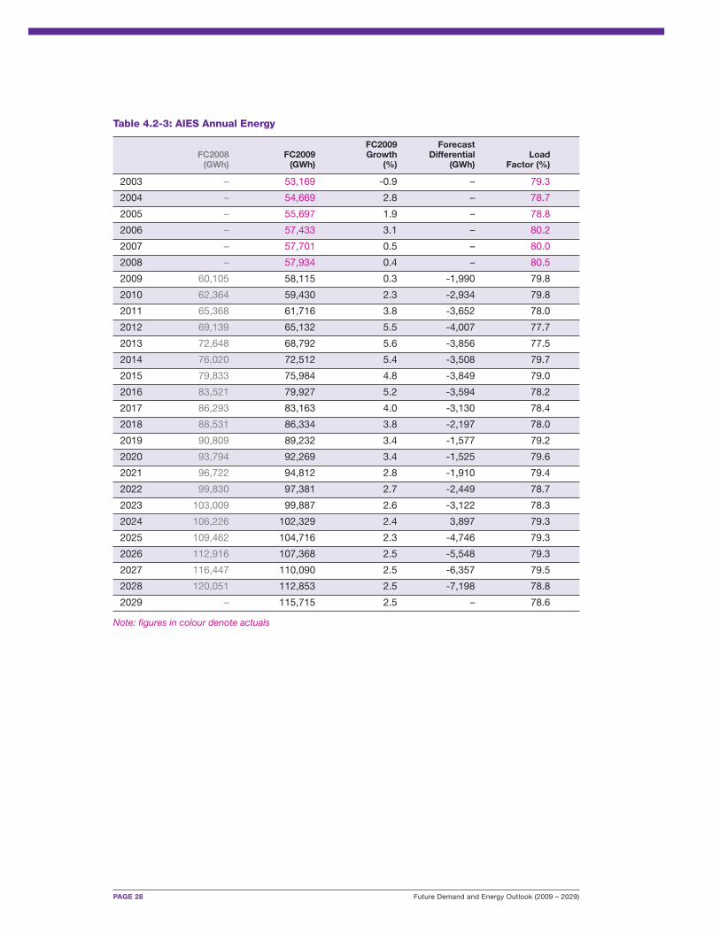
4.3 PROVINCIAL RESULTS – DEMAND TARIFF SERVICE (DTS) ENERGY
The AESO forecasts the annual energy amounts served to DTS customers. This value is AIES
minus transmission losses and Fort Nelson demand transmission service (FTS). The annual
amounts from 2010 and beyond are shown in Table 4.3-1 below.
Table 4.3-1: DTS Annual Energy
FC2009 FC2009(GWh) Growth (%)
2010 55,866 –
2011 58,177 4.1
2012 61,089 5.0
2013 64,875 6.2
2014 67,791 4.5
2015 70,369 3.8
2016 73,990 5.1
2017 77,054 4.1
2018 80,071 3.9
2019 82,815 3.4
2020 85,581 3.3
2021 87,567 2.3
2022 89,689 2.4
2023 91,996 2.6
2024 94,228 2.4
2025 96,574 2.5
2026 99,151 2.7
2027 101,789 2.7
2028 104,471 2.6
2029 107,259 2.7
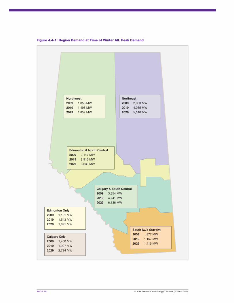
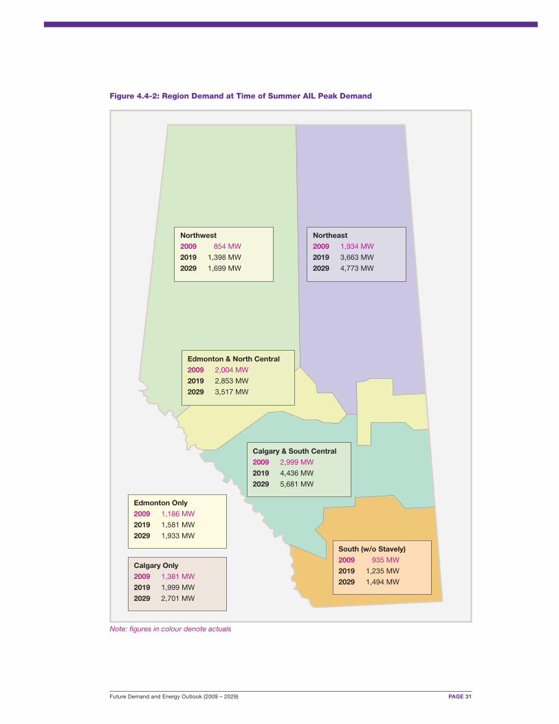
4.4 FORECAST RESULTS FOR BULK PLANNING PURPOSES
From a bulk transmission planning perspective, the AESO has defined five primary regions in
Alberta. There are also two large urban centres: Calgary and Edmonton.
Figure 4.4-1 shows the forecast regional winter peaks for 2009, 2019 and 2029 and Figure
4.4-2 shows the regional summer peaks for the same periods. In this case, the winter season is
the period from November 1 to April 30 and the summer season is from May 1 to October 31.
Strong growth in the Northeast, Calgary, and South Central regions is driven mainly by oilsands
and upgrading production forecasts for the northeast, and by increasing pipeline demand from
Hardisty south into the U.S. in the Calgary and South Central regions.
PAGE 30 Future Demand and Energy Outlook (2009 – 2029)
Figure 4.4-1: Region Demand at Time of Winter AIL Peak Demand
Northwest
2009 1,058 MW
2019 1,498 MW
2029 1,852 MW
Northeast
2009 2,063 MW
2019 4,035 MW
2029 5,140 MW
Edmonton & North Central
2009 2,147 MW
2019 2,916 MW
2029 3,630 MW
Calgary & South Central
2009 3,354 MW
2019 4,741 MW
2029 6,136 MW
Edmonton Only
2009 1,151 MW
2019 1,543 MW
2029 1,891 MW
South (w/o Stavely)
2009 877 MW
2019 1,157 MW
2029 1,415 MW
Calgary Only
2009 1,450 MW
2019 1,997 MW
2029 2,724 MW
Future Demand and Energy Outlook (2009 – 2029) PAGE 31
Figure 4.4-2: Region Demand at Time of Summer AIL Peak Demand
Northwest
2009 854 MW
2019 1,398 MW
2029 1,699 MW
Northeast
2009 1,934 MW
2019 3,663 MW
2029 4,773 MW
Edmonton & North Central
2009 2,004 MW
2019 2,853 MW
2029 3,517 MW
Calgary & South Central
2009 2,999 MW
2019 4,436 MW
2029 5,681 MW
Edmonton Only
2009 1,186 MW
2019 1,581 MW
2029 1,933 MW
South (w/o Stavely)
2009 935 MW
2019 1,235 MW
2029 1,494 MW
Calgary Only
2009 1,381 MW
2019 1,999 MW
2029 2,701 MW
Note: figures in colour denote actuals
PAGE 32 Future Demand and Energy Outlook (2009 – 2029)
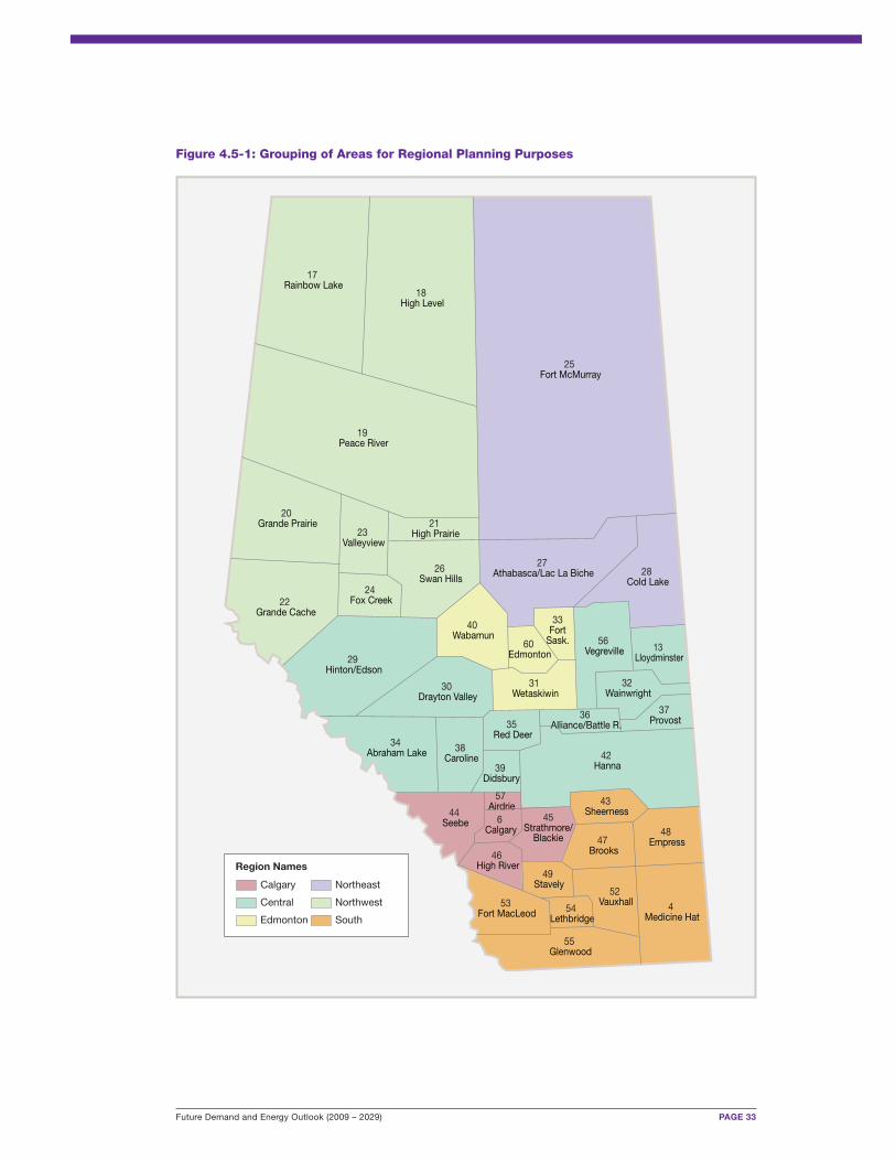
4.5 FORECAST RESULTS FOR REGIONAL PLANNING PURPOSES
The Province of Alberta covers over 661,100 square kilometres. This represents approximately
seven per cent of Canada’s total land mass. Given the considerable size of the province, it is
reasonable to expect the geography, economics and climate will vary from one region to another.
This geographical diversity is apparent in the AESO’s load forecast as seen in the tables that
follow. Figure 4.5-1 shows the province divided into areas. These areas can be added together
to explore electric power needs unique to that particular region.
For regional planning purposes, areas have been grouped to represent six regions: South,
Calgary, Central, Edmonton, Northeast and Northwest.
The following tables show regional peak demand coincident for both the summer and winter
seasons. The FC2009 results are compared to the forecast numbers for 2014, 2019 and 2029.
Future Demand and Energy Outlook (2009 – 2029) PAGE 33
Figure 4.5-1: Grouping of Areas for Regional Planning Purposes
25 Fort McMurray
19 Peace River
18 High Level
42 Hanna
17 Rainbow Lake
29 Hinton/Edson
22 Grande Cache
28 Cold Lake
20 Grande Prairie
26 Swan Hills
44 Seebe
4 Medicine Hat
55 Glenwood
34 Abraham Lake
56 Vegreville
40 Wabamun
27 Athabasca/Lac La Biche
48 Empress
30 Drayton Valley
47 Brooks
38 Caroline
52 Vauxhall
31 Wetaskiwin
53 Fort MacLeod
24 Fox Creek
32 Wainwright
35 Red Deer
49 Stavely
43 Sheerness
21 High Prairie23
Valleyview
37 Provost
13 Lloydminster
39 Didsbury
46 High River
60 Edmonton
6 Calgary
33Fort
Sask.
45Strathmore/
Blackie
54 Lethbridge
36 Alliance/Battle R.
57 Airdrie
Calgary
Central
Edmonton
Northeast
Northwest
South
Region Names
PAGE 34 Future Demand and Energy Outlook (2009 – 2029)
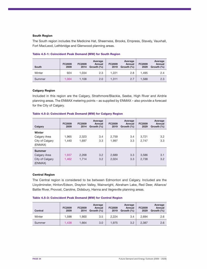
South Region
The South region includes the Medicine Hat, Sheerness, Brooks, Empress, Stavely, Vauxhall,
Fort MacLeod, Lethbridge and Glenwood planning areas.
Table 4.5-1: Coincident Peak Demand (MW) for South Region
Average Average AverageFC2009 FC2009 Annual FC2009 Annual FC2009 Annual
South 2009 2014 Growth (%) 2019 Growth (%) 2029 Growth (%)
Winter 924 1,034 2.3 1,221 2.8 1,495 2.4
Summer 1,004 1,108 2.0 1,311 2.7 1,588 2.3
Calgary Region
Included in this region are the Calgary, Strathmore/Blackie, Seebe, High River and Airdrie
planning areas. The ENMAX metering points – as supplied by ENMAX – also provide a forecast
for the City of Calgary.
Table 4.5-2: Coincident Peak Demand (MW) for Calgary Region
Average Average AverageFC2009 FC2009 Annual FC2009 Annual FC2009 Annual
Calgary 2009 2014 Growth (%) 2019 Growth (%) 2029 Growth (%)
WinterCalgary Area 1,965 2,323 3.4 2,759 3.4 3,721 3.2City of Calgary 1,440 1,697 3.3 1,997 3.3 2,747 3.3(ENMAX)
SummerCalgary Area 1,937 2,268 3.2 2,689 3.3 3,586 3.1City of Calgary 1,462 1,714 3.2 2,024 3.3 2,738 3.2(ENMAX)
Central Region
The Central region is considered to be between Edmonton and Calgary. Included are the
Lloydminster, Hinton/Edson, Drayton Valley, Wainwright, Abraham Lake, Red Deer, Alliance/
Battle River, Provost, Caroline, Didsbury, Hanna and Vegreville planning areas.
Table 4.5-3: Coincident Peak Demand (MW) for Central Region
Average Average AverageFC2009 FC2009 Annual FC2009 Annual FC2009 Annual
Central 2009 2014 Growth (%) 2019 Growth (%) 2029 Growth (%)
Winter 1,598 1,900 3.5 2,224 3.4 2,694 2.6
Summer 1,438 1,664 3.0 1,975 3.2 2,387 2.6
Future Demand and Energy Outlook (2009 – 2029) PAGE 35
Edmonton Region
Acting as a transmission hub, the Edmonton region includes the Wetaskiwin, Fort Saskatchewan,
Wabamun and Edmonton planning areas. The EPCOR metering points – as supplied by EPCOR
– also provide a forecast for the City of Edmonton.
Table 4.5-4: Coincident Peak Demand (MW) for Edmonton Region
Average Average AverageFC2009 FC2009 Annual FC2009 Annual FC2009 Annual
Edmonton 2009 2014 Growth (%) 2019 Growth (%) 2029 Growth (%)
WinterEdmonton Area 2,461 2,825 2.8 3,246 2.8 3,935 2.4City of Edmonton 1,199 1,335 2.2 1,572 2.7 1,906 2.3(EPCOR)
SummerEdmonton Area 2,457 2,704 1.9 3,134 2.5 3,788 2.2City of Edmonton 1,203 1,340 2.2 1,584 2.8 1,932 2.4(EPCOR)
Northeast Region
The Northeast region is forecast to experience the greatest demand and energy growth over
the next 10 years. This is due in large part to the oilsands industry. The Northeast region includes
the Fort McMurray, Athabasca/Lac La Biche and Cold Lake planning areas.
Table 4.5-5: Coincident Peak Demand (MW) for Northeast Region
Average Average AverageFC2009 FC2009 Annual FC2009 Annual FC2009 Annual
Northeast 2009 2014 Growth (%) 2019 Growth (%) 2029 Growth (%)
Winter 1,778 2,766 9.2 3,602 7.3 4,752 5.0
Summer 1,657 2,526 8.8 3,358 7.3 4,413 5.0
Northwest Region
The Northwest region includes the Rainbow Lake, High Level, Peace River, Grande Prairie,
High Prairie, Grand Cache, Valleyview, Fox Creek and Swan Hills planning areas.
Table 4.5-6: Coincident Peak Demand (MW) for Northwest Region
Average Average AverageFC2009 FC2009 Annual FC2009 Annual FC2009 Annual
Northwest 2009 2014 Growth (%) 2019 Growth (%) 2029 Growth (%)
Winter 1,100 1,363 4.4 1,570 3.6 1,898 2.8
Summer 1,059 1,255 3.5 1,459 3.3 1,740 2.5
PAGE 36 Future Demand and Energy Outlook (2009 – 2029)
5.0 Other Load Forecasting Considerations
In addition to the uncertainty associated with economic and demographic variables, there are
other significant challenges in developing a long-term load forecast for Alberta. Many of these
are addressed implicitly by the AESO’s load forecasting models. Although the factors discussed
below are not explicitly included in the load forecasting models, they are examined by the AESO
on a regular basis to inform the load forecasting process.
5.1 DEMAND RESPONSIVE LOAD AND CONSERVATION
The potential impact of conservation and efficiency (that will drive or be driven by the
advancement of new technologies), and demand responsive load programs represents an
additional source of uncertainty and challenge for the AESO’s load forecast. In general, these
can be programs that encourage conservation and efficiency, or programs that allow consumers
to respond to market signals and voluntarily reduce electricity consumption based on market
prices. Another change affecting the forecast relates to the direction given by the system
controller to facility owners during unexpected events such as supply shortfall in the form of
operational policy and procedures. With such programs, there is potential to reduce or shift the
timing of Alberta system peaks and energy requirements.
Current Alberta market design relies primarily on price signals to provide consumer incentives
for economically efficient electricity consumption and production decisions. Price responsive
load has been seen primarily from industrial customers that have flexible production such that
they can turn down operations and respond to high market prices. Depending on the market
price, the amount of price responsive load has ranged from 175 to 300 MW.
Future Demand and Energy Outlook (2009 – 2029) PAGE 37
The AESO has implemented a combination of demand response programs to assist in managing
or preventing emergency system operating conditions. These include:
� Voluntary load curtailment protocol (VLCP) – a demand response program based on
a pre-arranged contract.
� Demand opportunity service (DOS) – an opportunity transmission service with
regulated rates for each level of interruption (seven minutes and one hour).
� Frequency load shed service (FLSS) – load shed instantaneously during system events.
� Supplemental operating reserves (SUP) – Ancillary service available to arrest
frequency decline but not required to respond directly to frequency deviations.
This can be a load or generator service.
The net impact of these programs is captured in the AESO’s long-term load forecast modelling
processes. The forecasting models, which are based upon historical values, reflect the historical
effect of these programs. As a result, forecasted energy and peak demand values implicitly
include the effect of demand response programs.
There is a major emphasis on energy efficiency and conservation programs in various North
American jurisdictions, which are encompassed by the term demand side management (DSM).
DSM generally refers to activities that occur on the demand side of the meter, and are
implemented by the customer directly or by load serving entities. DSM initiatives are aimed at
achieving energy savings as a result of conservation, energy efficiency and load displacement
programs. A substantial portion of these energy savings has resulted from appliance and
building standards. Another major portion of savings are utility programs mandated by
governments and regulators, including efficiency services in the form of energy audits, financial
incentive, load-shifting activities and rate design.
Several jurisdictions are implementing very aggressive DSM programs including California, the
U.S. Pacific Northwest and B.C. For example, BC Hydro is required to acquire 50 per cent of
its incremental resource needs through conservation (DSM) by 2020. The approach adopted to
load forecasting in these jurisdictions typically involves a detailed assessment of the impact of
DSM programs and price effects on electricity demand. These analytical requirements
characteristically necessitate an extremely detailed end-use approach to demand forecasting.
To date, load-serving entities or retailers in Alberta have not developed price responsive,
efficiency or conservation programs in the same way as other jurisdictions, especially those
that rely on the traditional integrated utility model. Consequently, reduction in demand
opportunities from this sector to date have been negligible. The potential impacts of demand
response and DSM-type programs are not explicitly included in the AESO’s load-forecasting
models, given that such programs are not widespread and future programs are unknown at this
time. The AESO will continue to evaluate appropriate programs related to DSM.
PAGE 38 Future Demand and Energy Outlook (2009 – 2029)
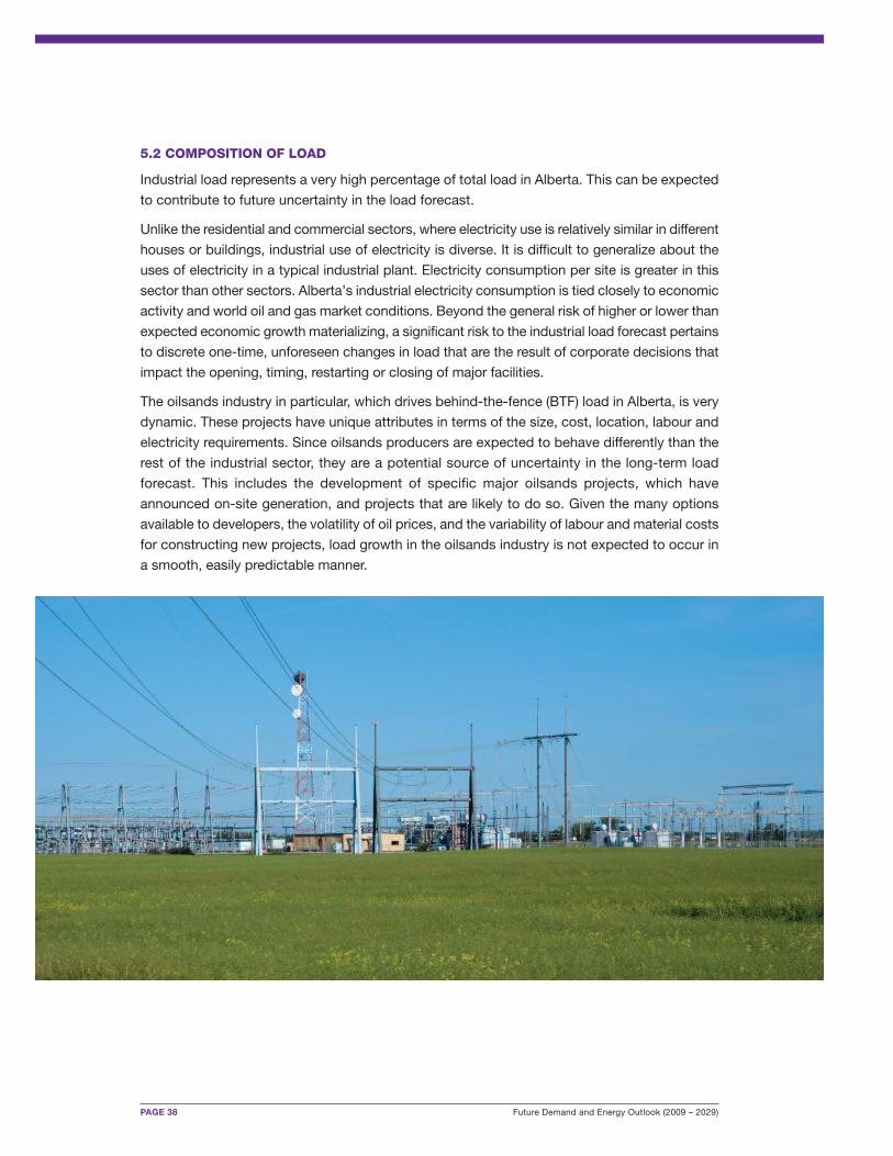
5.2 COMPOSITION OF LOAD
Industrial load represents a very high percentage of total load in Alberta. This can be expected
to contribute to future uncertainty in the load forecast.
Unlike the residential and commercial sectors, where electricity use is relatively similar in different
houses or buildings, industrial use of electricity is diverse. It is difficult to generalize about the
uses of electricity in a typical industrial plant. Electricity consumption per site is greater in this
sector than other sectors. Alberta’s industrial electricity consumption is tied closely to economic
activity and world oil and gas market conditions. Beyond the general risk of higher or lower than
expected economic growth materializing, a significant risk to the industrial load forecast pertains
to discrete one-time, unforeseen changes in load that are the result of corporate decisions that
impact the opening, timing, restarting or closing of major facilities.
The oilsands industry in particular, which drives behind-the-fence (BTF) load in Alberta, is very
dynamic. These projects have unique attributes in terms of the size, cost, location, labour and
electricity requirements. Since oilsands producers are expected to behave differently than the
rest of the industrial sector, they are a potential source of uncertainty in the long-term load
forecast. This includes the development of specific major oilsands projects, which have
announced on-site generation, and projects that are likely to do so. Given the many options
available to developers, the volatility of oil prices, and the variability of labour and material costs
for constructing new projects, load growth in the oilsands industry is not expected to occur in
a smooth, easily predictable manner.
Future Demand and Energy Outlook (2009 – 2029) PAGE 39
5.3 DISTRIBUTED GENERATION
Distributed generation involves the installation of small-scale power sources at or near a customer’s
site to provide an alternative to, or an enhancement of, the traditional electric power system.
For generation smaller than 150 kW, modelling and forecasting of this generation and the load
that it offsets is not specifically tracked. Advanced Metering Infrastructure (AMI) and smart grid
could facilitate specific tracking of micro and other generation. It is assumed that the impact of
any potential drop in load caused by distributed generation will be captured through trends
seen in the econometric modelling of electricity consumption by sector. Major shifts can be
addressed as they are identified.
5.4 ENVIRONMENTAL COSTS
The costs of meeting environmental requirements are expected to rise across North America,
particularly for large greenhouse gas (GHG) emitters. While this may have an impact on the
in-service dates for some oilsands and upgrader projects, at this time there is no basis for
assuming these costs will significantly slow expansion in Alberta’s energy producing sectors.
Because it is unlikely that reduction in GHG emissions will occur without cost, future climate
control policy is a risk of uncertain magnitude and timing to the load forecast. Load forecasting
models used in other jurisdictions generally tend to use a fuel carbon content tax as a proxy
for the cost of mandated GHG reductions, whatever the means of implementation.
It can be expected that any costs associated with meeting environmental requirements for
electricity generation facilities in the future will ultimately be reflected in electricity prices. As
previously discussed, the AESO’s load-forecasting models do not explicitly include the influence
of electricity prices on electricity demand. However, any changes in demand patterns are
captured through the modelling process that accounts for historic trends that capture various
econometric drivers.

PAGE 40 Future Demand and Energy Outlook (2009 – 2029)
5.5 CHALLENGES ON THE HORIZON
This year a number of future challenges have been identified:
� New DSM initiatives, including demand response programs.
� New technology with different electricity intensities.
� New environmental regulations around GHG.
� New vehicle technology, including plug-in electric cars.
Each of these challenges will be explored in the coming year to determine their significance
with respect to the fundamental relationships that form the basis of the AESO’s Future Demand
and Energy Outlook (2009 – 2029).
Future Demand and Energy Outlook (2009 – 2029) PAGE 41
6.0 Historical and Past Forecast Results
In the process of preparing the long-term load forecast, the AESO assesses past forecasts
along with Alberta’s actual demand and electricity usage to verify methodology and identify
variances that could impact the current forecast.
6.1 PAST FORECAST VARIANCES
Table 6.1-1: Energy Forecast Variance History
Actuals Year-over- FC2005 FC2006 FC2007 FC2008Year (GWh) Year Change (%) (%) (%) (%)
2006 69,371 – -1 +1. – –
2007 69,660 +290 -3 -1 -1 –
2008 69,947 +286 -7 -4 -4 -1
2009 70,150 +204 -9 -7 -8 -4(FC2009)
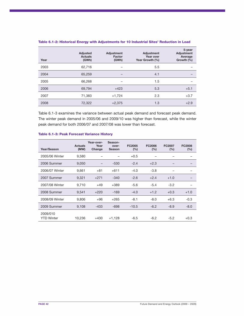
As noted in Section 3.7, a reduction in demand at 10 industrial sites contributed to a reduction
in energy growth in the province at the same time as strong growth in the oilsands and a strong
economy created energy growth in other customer sectors and industries. To quantify the effect
this drop in electricity consumption has had on energy growth, the AESO adjusted historical
energy values by adding an Adjustment Factor equal to the difference between the sum of
energy at these sites in 2005 minus the sum of energy at these sites in each historical year. The
year 2005 was used as a representative year in this analysis to calculate a baseline. The results
are shown in Table 6.1-2.
PAGE 42 Future Demand and Energy Outlook (2009 – 2029)
Table 6.1-2: Historical Energy with Adjustments for 10 Industrial Sites’ Reduction in Load
5-yearAdjusted Adjustment Adjustment AdjustmentActuals Factor Year over Average
Year (GWh) (GWh) Year Growth (%) Growth (%)
2003 62,716 – 5.5 –
2004 65,259 – 4.1 –
2005 66,268 – 1.5 –
2006 69,794 +423 5.3 +5.1
2007 71,383 +1,724 2.3 +3.7
2008 72,322 +2,375 1.3 +2.9
Table 6.1-3 examines the variance between actual peak demand and forecast peak demand.
The winter peak demand in 2005/06 and 2009/10 was higher than forecast, while the winter
peak demand for both 2006/07 and 2007/08 was lower than forecast.
Table 6.1-3: Peak Forecast Variance History
Year-over- Season-Actuals Year over- FC2005 FC2006 FC2007 FC2008
Year/Season (MW) Change Season (%) (%) (%) (%)
2005/06 Winter 9,580 – – +0.5 – – –
2006 Summer 9,050 – -530 -2.4 +2.3 – –
2006/07 Winter 9,661 +81 +611 -4.0 -3.8 – –
2007 Summer 9,321 +271 -340 -2.6 +2.4 +1.0 –
2007/08 Winter 9,710 +49 +389 -5.6 -5.4 -3.2 –
2008 Summer 9,541 +220 -169 -4.0 +1.2 +0.3 +1.0
2008/09 Winter 9,806 +96 +265 -8.1 -8.0 +6.3 -0.3
2009 Summer 9,108 -433 -698 -10.5 -6.2 -8.9 -8.0
2009/010 YTD Winter 10,236 +430 +1,128 -6.5 -6.2 -5.2 +0.3
Future Demand and Energy Outlook (2009 – 2029) PAGE 43
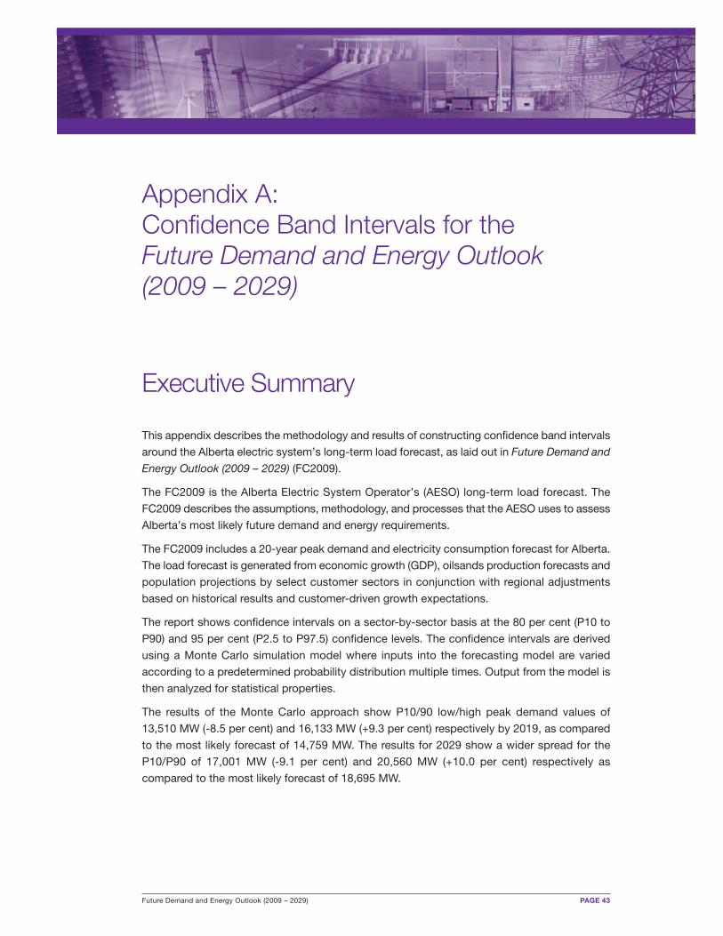
Appendix A: Confidence Band Intervals for the Future Demand and Energy Outlook(2009 – 2029)
Executive Summary
This appendix describes the methodology and results of constructing confidence band intervals
around the Alberta electric system’s long-term load forecast, as laid out in Future Demand and
Energy Outlook (2009 – 2029) (FC2009).
The FC2009 is the Alberta Electric System Operator’s (AESO) long-term load forecast. The
FC2009 describes the assumptions, methodology, and processes that the AESO uses to assess
Alberta’s most likely future demand and energy requirements.
The FC2009 includes a 20-year peak demand and electricity consumption forecast for Alberta.
The load forecast is generated from economic growth (GDP), oilsands production forecasts and
population projections by select customer sectors in conjunction with regional adjustments
based on historical results and customer-driven growth expectations.
The report shows confidence intervals on a sector-by-sector basis at the 80 per cent (P10 to
P90) and 95 per cent (P2.5 to P97.5) confidence levels. The confidence intervals are derived
using a Monte Carlo simulation model where inputs into the forecasting model are varied
according to a predetermined probability distribution multiple times. Output from the model is
then analyzed for statistical properties.
The results of the Monte Carlo approach show P10/90 low/high peak demand values of
13,510 MW (-8.5 per cent) and 16,133 MW (+9.3 per cent) respectively by 2019, as compared
to the most likely forecast of 14,759 MW. The results for 2029 show a wider spread for the
P10/P90 of 17,001 MW (-9.1 per cent) and 20,560 MW (+10.0 per cent) respectively as
compared to the most likely forecast of 18,695 MW.
PAGE 44 Future Demand and Energy Outlook (2009 – 2029)
1.0 Introduction
The AESO’s long-term load forecast is a study of past energy use patterns and future economic
indicators that are combined to produce a future energy forecast. The AESO annually updates
this energy forecast with a 20-year outlook of Alberta’s electric consumption and peak demand.
The estimates of future electricity market needs are one of the drivers the AESO uses in
analyzing and planning the timely development of the transmission system. The annual forecast
is based on economic, demographic and customer information collected from January through
June of 2009.
The FC2009 describes the assumptions, methodology and processes that the AESO employs
to assess Alberta’s most likely future demand and energy requirements.
Along with its long-term load forecast, the AESO requires high and low confidence bands that
reflect a reasonable expected range of the forecast. Potential sources of error exist with any
forecast and it is important to recognize and attempt to measure the potential effect that any
error may have on the forecast. The assumptions used and the underlying methodology of
forecasting are explained to justify why the confidence bands represent a relatively likely forecast.
Forecasts cannot precisely predict the future. Variation in the key factors that drive electrical
usage may deviate actual demand from forecast demand in any given year. To account for this,
the AESO reports its energy and demand forecast as a baseline or most likely outcome, as well
as a range of possible outcomes based on probabilities around the base case. For planning
and analytical purposes, it is useful to have an estimate not only of the most likely case but
also of the distribution of probabilities around the forecast.
The AESO developed upper and lower confidence bands around the 2009 load forecast for
each sector. The P2.5/P97.5 confidence band corresponds to a 95 per cent confidence interval.
This means there is a 95 per cent chance that the actual energy demand will fall within this
interval and there is a five per cent chance actual demand will fall outside this interval. Similarly,
the P10/P90 confidence band corresponds to an 80 per cent confidence interval for which there
is an 80 per cent chance that the forecast will fall within its bands.
A Monte Carlo simulation method was used to calculate confidence band intervals for each
sector as well as for total Alberta internal load (AIL) and peak demand. Monte Carlo simulations
vary the inputs into the forecasting models according to a calculated probability distribution
based on historical data. Output results from the model are then analyzed for their statistical
properties to determine the confidence intervals. This method of determining confidence bands
has the advantage of varying all the factors that affect electricity use and demand according
to their historical tendencies multiple times so actual variation in the forecast can be measured
and analyzed.
Future Demand and Energy Outlook (2009 – 2029) PAGE 45
2.0 Monte Carlo Analysis
Monte Carlo simulations were performed individually on all five sector models as well as on an
aggregated model, which combines all the sectors together. Within the models there are
econometrically forecasted coefficients as well as externally-forecast values of input variables.
All variables are allowed to vary according to defined probability distributions that are based on
historical data wherever possible. It should be noted that in many instances historical data was
not available, or was not adequate to produce a reasonable probability distribution estimate. In
these instances, the AESO formulated its own estimate of probability distribution using the
forecast values plus a reasonable assessment of potential variation for those forecast values.
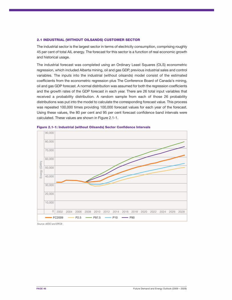
PAGE 46 Future Demand and Energy Outlook (2009 – 2029)
90,000
80,000
70,000
60,000
50,000
40,000
30,000
20,000
10,000
0
Source: AESO and ERCB
Ene
rgy
(GW
h)
Figure 2.1-1: Industrial (without Oilsands) Sector Confidence Intervals
FC2009 P2.5 P97.5 P10 P90
2002 2004 2006 2008 2010 2012 2014 2016 2018 2020 2022 2024 2026 2028
2.1 INDUSTRIAL (WITHOUT OILSANDS) CUSTOMER SECTOR
The industrial sector is the largest sector in terms of electricity consumption, comprising roughly
45 per cent of total AIL energy. The forecast for this sector is a function of real economic growth
and historical usage.
The industrial forecast was completed using an Ordinary Least Squares (OLS) econometric
regression, which included Alberta mining, oil and gas GDP, previous industrial sales and control
variables. The inputs into the industrial (without oilsands) model consist of the estimated
coefficients from the econometric regression plus The Conference Board of Canada’s mining,
oil and gas GDP forecast. A normal distribution was assumed for both the regression coefficients
and the growth rates of the GDP forecast in each year. There are 26 total input variables that
received a probability distribution. A random sample from each of those 26 probability
distributions was put into the model to calculate the corresponding forecast value. This process
was repeated 100,000 times providing 100,000 forecast values for each year of the forecast.
Using these values, the 80 per cent and 95 per cent forecast confidence band intervals were
calculated. These values are shown in Figure 2.1-1.
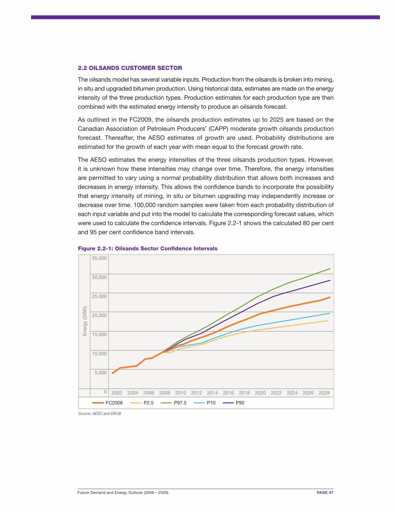
Future Demand and Energy Outlook (2009 – 2029) PAGE 47
2.2 OILSANDS CUSTOMER SECTOR
The oilsands model has several variable inputs. Production from the oilsands is broken into mining,
in situ and upgraded bitumen production. Using historical data, estimates are made on the energy
intensity of the three production types. Production estimates for each production type are then
combined with the estimated energy intensity to produce an oilsands forecast.
As outlined in the FC2009, the oilsands production estimates up to 2025 are based on the
Canadian Association of Petroleum Producers’ (CAPP) moderate growth oilsands production
forecast. Thereafter, the AESO estimates of growth are used. Probability distributions are
estimated for the growth of each year with mean equal to the forecast growth rate.
The AESO estimates the energy intensities of the three oilsands production types. However,
it is unknown how these intensities may change over time. Therefore, the energy intensities
are permitted to vary using a normal probability distribution that allows both increases and
decreases in energy intensity. This allows the confidence bands to incorporate the possibility
that energy intensity of mining, in situ or bitumen upgrading may independently increase or
decrease over time. 100,000 random samples were taken from each probability distribution of
each input variable and put into the model to calculate the corresponding forecast values, which
were used to calculate the confidence intervals. Figure 2.2-1 shows the calculated 80 per cent
and 95 per cent confidence band intervals.
35,000
30,000
25,000
20,000
15,000
10,000
5,000
0
Source: AESO and ERCB
Ene
rgy
(GW
h)
Figure 2.2-1: Oilsands Sector Confidence Intervals
FC2008 P2.5 P97.5 P10 P90
2002 2004 2006 2008 2010 2012 2014 2016 2018 2020 2022 2024 2026 2028
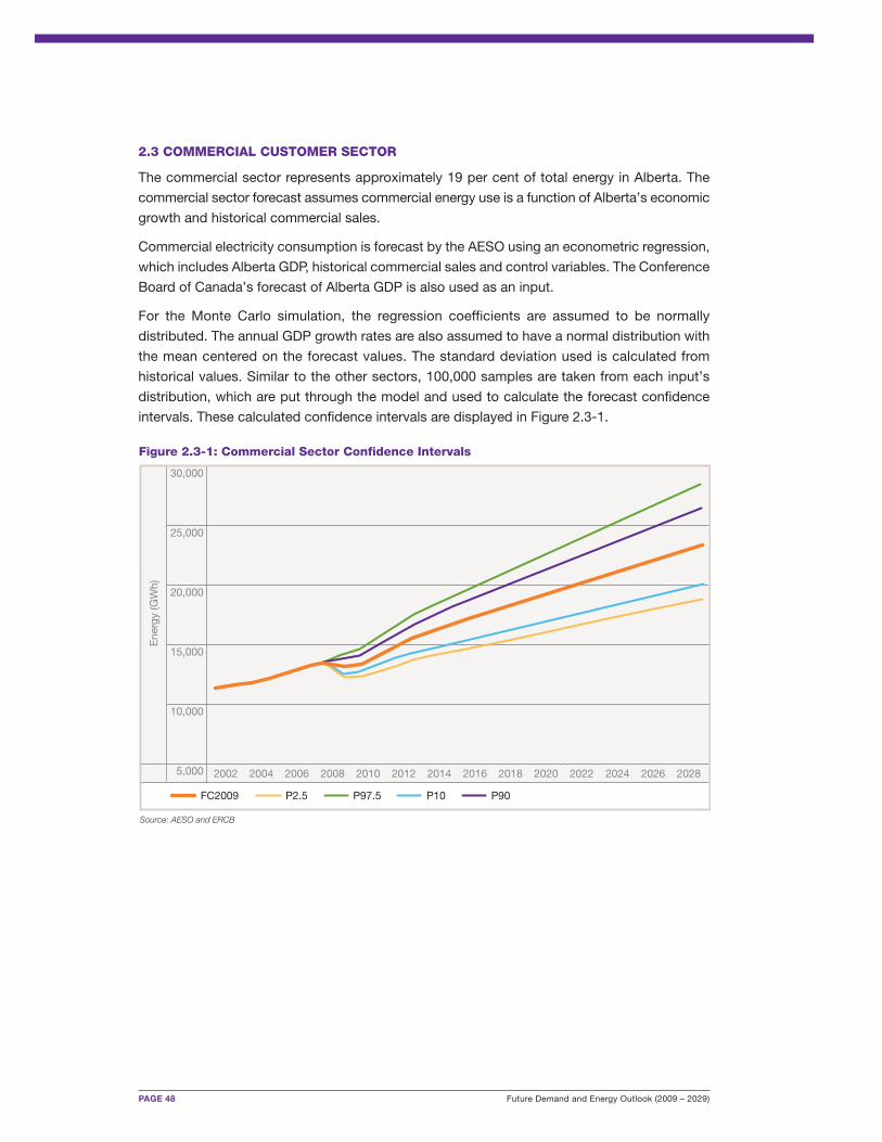
PAGE 48 Future Demand and Energy Outlook (2009 – 2029)
2.3 COMMERCIAL CUSTOMER SECTOR
The commercial sector represents approximately 19 per cent of total energy in Alberta. The
commercial sector forecast assumes commercial energy use is a function of Alberta’s economic
growth and historical commercial sales.
Commercial electricity consumption is forecast by the AESO using an econometric regression,
which includes Alberta GDP, historical commercial sales and control variables. The Conference
Board of Canada’s forecast of Alberta GDP is also used as an input.
For the Monte Carlo simulation, the regression coefficients are assumed to be normally
distributed. The annual GDP growth rates are also assumed to have a normal distribution with
the mean centered on the forecast values. The standard deviation used is calculated from
historical values. Similar to the other sectors, 100,000 samples are taken from each input’s
distribution, which are put through the model and used to calculate the forecast confidence
intervals. These calculated confidence intervals are displayed in Figure 2.3-1.
30,000
25,000
20,000
15,000
10,000
5,000
Source: AESO and ERCB
Ene
rgy
(GW
h)
Figure 2.3-1: Commercial Sector Confidence Intervals
FC2009 P2.5 P97.5 P10 P90
2002 2004 2006 2008 2010 2012 2014 2016 2018 2020 2022 2024 2026 2028
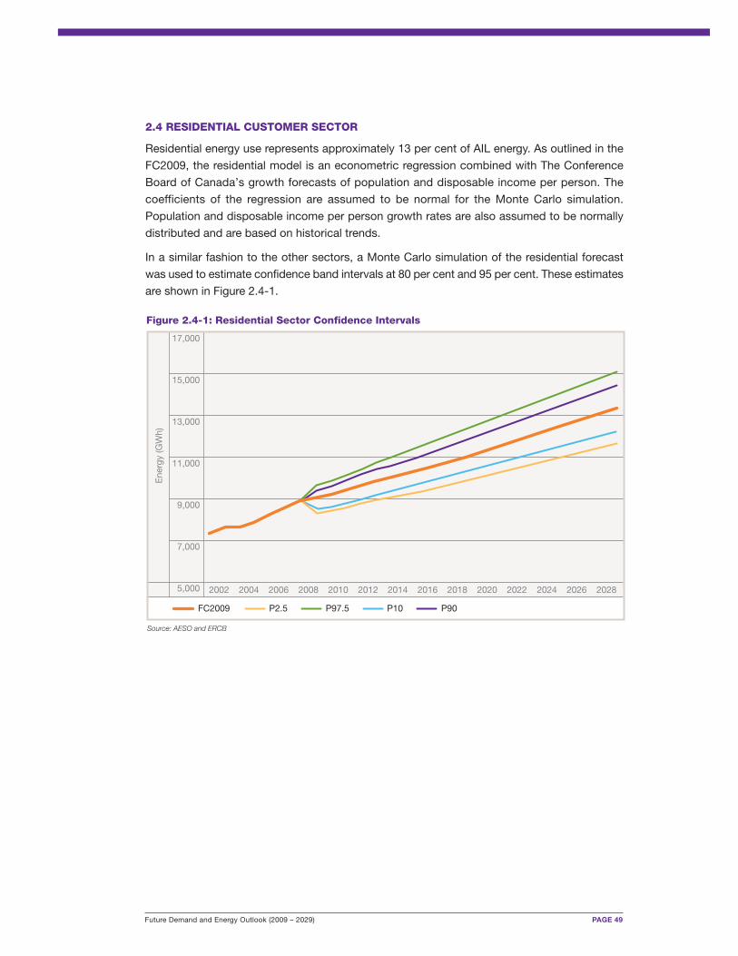
Future Demand and Energy Outlook (2009 – 2029) PAGE 49
2.4 RESIDENTIAL CUSTOMER SECTOR
Residential energy use represents approximately 13 per cent of AIL energy. As outlined in the
FC2009, the residential model is an econometric regression combined with The Conference
Board of Canada’s growth forecasts of population and disposable income per person. The
coefficients of the regression are assumed to be normal for the Monte Carlo simulation.
Population and disposable income per person growth rates are also assumed to be normally
distributed and are based on historical trends.
In a similar fashion to the other sectors, a Monte Carlo simulation of the residential forecast
was used to estimate confidence band intervals at 80 per cent and 95 per cent. These estimates
are shown in Figure 2.4-1.
17,000
15,000
13,000
11,000
9,000
7,000
5,000
Source: AESO and ERCB
Ene
rgy
(GW
h)
Figure 2.4-1: Residential Sector Confidence Intervals
FC2009 P2.5 P97.5 P10 P90
2002 2004 2006 2008 2010 2012 2014 2016 2018 2020 2022 2024 2026 2028
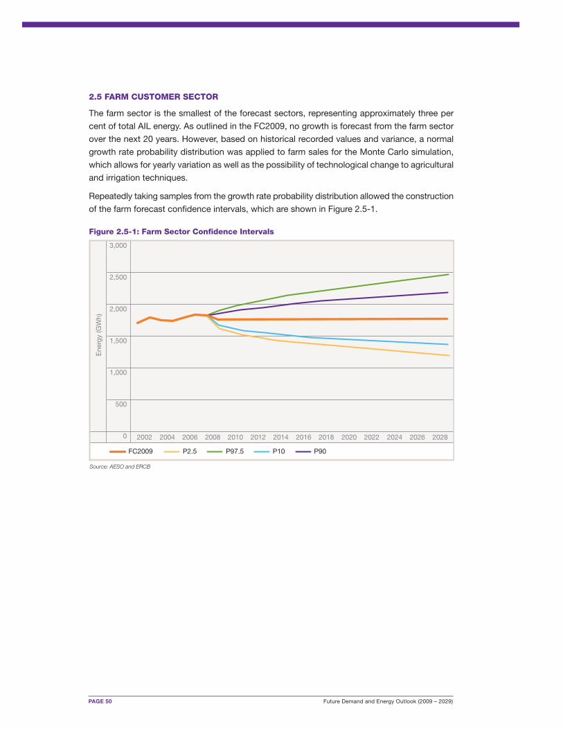
PAGE 50 Future Demand and Energy Outlook (2009 – 2029)
2.5 FARM CUSTOMER SECTOR
The farm sector is the smallest of the forecast sectors, representing approximately three per
cent of total AIL energy. As outlined in the FC2009, no growth is forecast from the farm sector
over the next 20 years. However, based on historical recorded values and variance, a normal
growth rate probability distribution was applied to farm sales for the Monte Carlo simulation,
which allows for yearly variation as well as the possibility of technological change to agricultural
and irrigation techniques.
Repeatedly taking samples from the growth rate probability distribution allowed the construction
of the farm forecast confidence intervals, which are shown in Figure 2.5-1.
3,000
2,500
2,000
1,500
1,000
500
0
Source: AESO and ERCB
Ene
rgy
(GW
h)
Figure 2.5-1: Farm Sector Confidence Intervals
FC2009 P2.5 P97.5 P10 P90
2002 2004 2006 2008 2010 2012 2014 2016 2018 2020 2022 2024 2026 2028
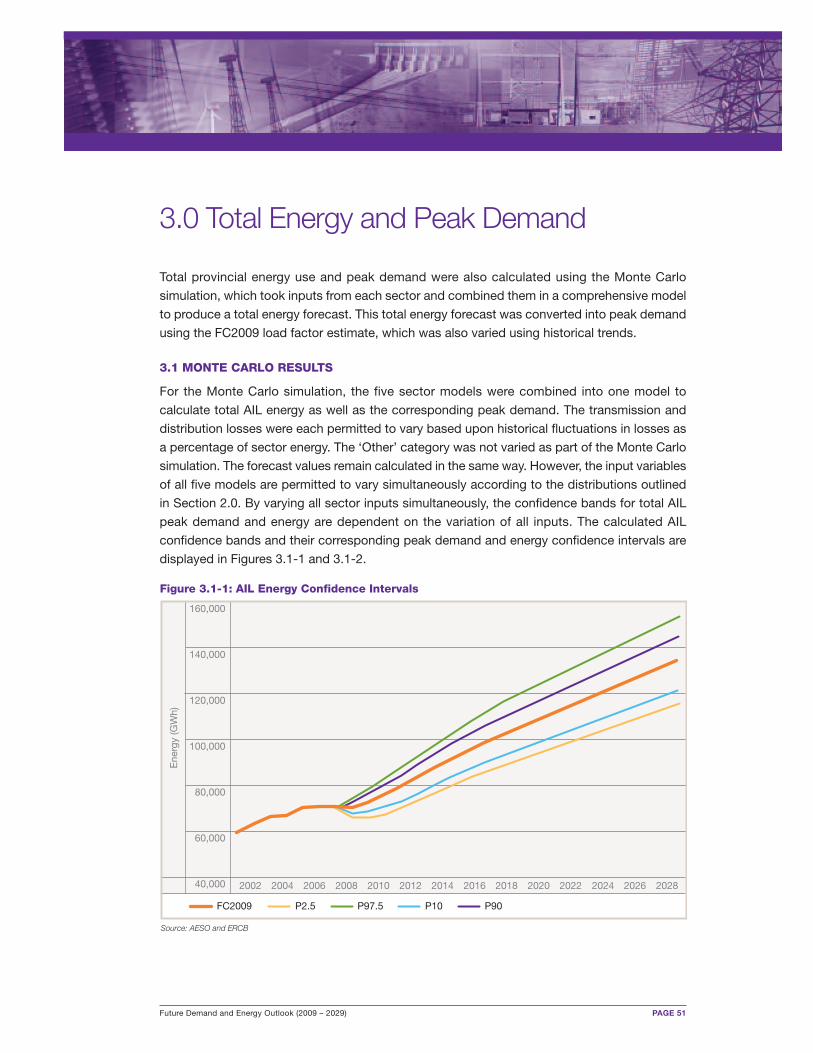
Future Demand and Energy Outlook (2009 – 2029) PAGE 51
3.0 Total Energy and Peak Demand
Total provincial energy use and peak demand were also calculated using the Monte Carlo
simulation, which took inputs from each sector and combined them in a comprehensive model
to produce a total energy forecast. This total energy forecast was converted into peak demand
using the FC2009 load factor estimate, which was also varied using historical trends.
3.1 MONTE CARLO RESULTS
For the Monte Carlo simulation, the five sector models were combined into one model to
calculate total AIL energy as well as the corresponding peak demand. The transmission and
distribution losses were each permitted to vary based upon historical fluctuations in losses as
a percentage of sector energy. The ‘Other’ category was not varied as part of the Monte Carlo
simulation. The forecast values remain calculated in the same way. However, the input variables
of all five models are permitted to vary simultaneously according to the distributions outlined
in Section 2.0. By varying all sector inputs simultaneously, the confidence bands for total AIL
peak demand and energy are dependent on the variation of all inputs. The calculated AIL
confidence bands and their corresponding peak demand and energy confidence intervals are
displayed in Figures 3.1-1 and 3.1-2.
160,000
140,000
120,000
100,000
80,000
60,000
40,000
Source: AESO and ERCB
Ene
rgy
(GW
h)
Figure 3.1-1: AIL Energy Confidence Intervals
FC2009 P2.5 P97.5 P10 P90
2002 2004 2006 2008 2010 2012 2014 2016 2018 2020 2022 2024 2026 2028
PAGE 52 Future Demand and Energy Outlook (2009 – 2029)
Tables 3.1-1 and 3.1-2 report the confidence interval results from the Monte Carlo simulation
on AIL energy and peak demand respectively. The results of the Monte Carlo approach
show P10/90 low/high peak demand values of 13,510 MW (-8.5 per cent) and 16,133 MW
(+9.3 per cent) respectively by 2019 as compared to the most likely forecast of 14,759 MW.
The results for 2029 show a wider spread for the P10/P90 of 17,001 MW (-9.1 per cent) and
20,560 MW (+10.0 per cent) respectively as compared to the most likely forecast of 18,695 MW.
24,000
22,000
20,000
18,000
16,000
14,000
12,000
10,000
8,000
6,000
Source: AESO and ERCB
Pea
k D
eman
d (M
W)
Figure 3.1-2: AIL Winter Peak Demand Confidence Intervals
FC2009 P2.5 P97.5 P10 P90
2002 2004 2006 2008 2010 2012 2014 2016 2018 2020 2022 2024 2026 2028
Future Demand and Energy Outlook (2009 – 2029) PAGE 53
Additional analysis indicates that by 2029, the largest source of variation in the AIL energy
forecast will come from the industrial sector. Specifically, the coefficient on the mining, oil and
gas GDP contributes most to overall variation. While statistically significant, the coefficient had
a relatively high standard error resulting both from fairly low degrees of freedom (because of a
relatively low number of annual observations) and from a recent historical divergence of
industrial energy use and mining, oil and gas GDP. As discussed in the FC2009, the decrease
in industrial energy use resulted from the exit and decrease in activity of several non-oil and
gas-related firms that are not part of mining, oil and gas GDP.
Going forward, it is expected that industrial energy use will continue to increase with mining,
oil and gas GDP since the majority of industrial energy use is by the oil and gas sector. However,
because of the recent industrial decline, certainty surrounding the coefficient on mining, oil and
gas GDP is less assured. This creates additional variation in the industrial (without oilsands)
sector confidence bands. Since the industrial (without oilsands) sector is the largest component
of AIL energy, it also creates the largest source of variation in the total AIL energy forecast
confidence bands. Given the difficulty to predict the exit or decrease in activity of industrial
firms, this higher variation seen in the industrial sector seems appropriate.
PAGE 54 Future Demand and Energy Outlook (2009 – 2029)
Table 3.1-1: AIL Energy Confidence Intervals
FC2009 P97.5 P90 P10 P2.5(GWh) (GWh) (GWh) (GWh) (GWh)
2009 70,184 74,391 72,903 67,426 66,001
2010 72,459 78,845 76,573 68,466 66,423
2011 75,312 83,270 80,438 70,451 67,961
2012 78,963 88,164 84,866 73,416 70,577
2013 82,877 93,101 89,459 76,738 73,632
2014 86,965 98,221 94,160 80,289 76,922
2015 90,900 103,019 98,638 83,779 80,190
2016 95,335 108,284 103,556 87,740 83,877
2017 98,870 112,585 107,593 90,867 86,827
2018 102,220 116,613 111,369 93,831 89,642
2019 105,344 120,318 114,887 96,640 92,260
2020 108,638 124,304 118,598 99,619 95,059
2021 111,208 127,305 121,479 101,866 97,144
2022 113,923 130,567 124,516 104,264 99,478
2023 116,691 133,939 127,608 106,731 101,722
2024 119,261 136,845 130,501 109,051 103,890
2025 121,640 139,811 133,207 111,164 105,845
2026 124,355 143,038 136,247 113,528 108,115
2027 127,096 146,394 139,288 115,957 110,401
2028 129,911 149,609 142,463 118,451 112,687
2029 132,746 153,145 145,620 120,979 115,096
Future Demand and Energy Outlook (2009 – 2029) PAGE 55
Table 3.1-2: AIL Winter Peak Demand Confidence Intervals
FC2009 P97.5 P90 P10 P2.5MW MW MW MW MW
2009/10 9,846 10,519 10,284 9,422 9,201
2010/11 10,170 11,124 10,788 9,579 9,281
2011/12 10,577 11,746 11,328 9,866 9,503
2012/13 11,076 12,418 11,938 10,270 9,870
2013/14 11,664 13,155 12,620 10,776 10,329
2014/15 12,162 13,782 13,200 11,201 10,718
2015/16 12,801 14,553 13,923 11,774 11,260
2016/17 13,382 15,254 14,576 12,288 11,730
2017/18 13,856 15,828 15,113 12,704 12,132
2018/19 14,351 16,419 15,671 13,146 12,537
2019/20 14,759 16,923 16,133 13,510 12,883
2020/21 15,162 17,394 16,590 13,872 13,221
2021/22 15,618 17,944 17,098 14,271 13,588
2022/23 15,994 18,397 17,520 14,607 13,911
2023/24 16,369 18,838 17,942 14,943 14,225
2024/25 16,725 19,254 18,341 15,259 14,532
2025/26 17,114 19,741 18,782 15,600 14,848
2026/27 17,505 20,203 19,221 15,957 15,173
2027/28 17,855 20,638 19,608 16,257 15,465
2028/29 18,196 21,032 19,999 16,561 15,747
2029/30 18,695 21,625 20,560 17,001 16,156
PAGE 56 Future Demand and Energy Outlook (2009 – 2029)
List of Reference Documents
Alberta Employment, Immigration, and Industry (December 2008)
Monthly Economic Review
Energy Resources and Conservation Board
Alberta’s Energy Reserves 2009 and Supply/Demand Outlook 2009 – 2018 (ST98-2009)
Energy Resources and Conservation Board
Table 11: Electric Energy Distribution Sales and Number of Customers
Canadian Association of Petroleum Producers (June 2009)
Crude Oil Forecast, Markets and Pipeline Expansions
The Conference Board of Canada (2009)
Provincial Outlook Long-term Economic Forecast: 2009
The Conference Board of Canada (2009)
Provincial Outlook Spring 2009
National Energy Board (June 2006)
Canada’s Oil Sands – Opportunities and Challenges to 2015: An Update. (Review only)
Statistics Canada (December 2008)
Retail Sales by Industry (monthly)
Statistics Canada (March 2009)
Alberta Gross Domestic Product at Basic Prices by Industry (annual)
Statistics Canada (March 2009)
Alberta Population (annual)
Future Demand and Energy Outlook (2009 – 2029) PAGE 57
Glossary
Alberta Interconnected Electric System (AIES): the system of interconnected transmission
power lines and generators.
Alberta internal load (AIL): the total electricity consumption including behind-the-fence, the
City of Medicine Hat and losses (transmission and distribution).
Behind-the-fence load (BTF): industrial load characterized by being served in whole, or inpart, by on-site generation.
Bulk transmission system: the integrated system of transmission lines and substations that
delivers electric power from major generating stations to load centers. The bulk system, which
generally includes the 240 kV and 500 kV transmission lines and substations, also delivers/
receives power to and from adjacent power systems.
Capacity: amount of electric power delivered or required for a generator, turbine, transformer,
transmission circuit, substation or system as rated by the manufacturer.
Customer sectors: used to classify types of load. For the purposes of this report, five sectorswere used: industrial (without oilsands), oilsands, residential, commercial and farm.
Demand (coincident demand): a maximum electricity load in a given period of time for a
defined area with the units kW (kilowatt) or MW (megawatt).
Demand responsive load or price responsive load: large commercial and industrial
customers with flexibility in their operations that enables them to reduce load or demand in
response to market price signals or other directions from a system controller.
Demand side management (DSM): generally refers to activities that occur on the demand
side of the meter that are implemented by the customer directly or by load serving entities.
Energy: electricity consumption over a given period of time for a defined area with the units kWh
(kilowatt hour), MWh (megawatt hour) or GWh (gigawatt hour).
Gigawatt hour (GWh): one billion watt hours.
PAGE 58 Future Demand and Energy Outlook (2009 – 2029)
Gross domestic product (GDP): one of the measures of national income and output for a given
country’s economy. GDP is defined as the total market value of all final goods and services
produced within the country in a given period of time (usually a calendar year). It is also
considered the sum of a value added at every stage of production (the intermediate stages) of
all final goods and services produced within a country in a given period of time, and it is given
a monetary value.
Load factor: ratio of average power demand (load) to peak load during a specified period of
time; sometimes expressed as a per cent.
Megawatt (MW): one million Watts.
Metering point identifier (MP_ID): defined point of connection on the transmission provider’s
system where capacity and/or energy are made available to the end user.
Seasonal coincident peak: a coincident peak measured within a specific period of time defined
as a season; typically summer and winter are used but fall and spring can be included as well.
Substation/switching station: a facility where equipment is used to tie together two or more
electric circuits through switches (circuit breakers). The switches are selectively arranged to
permit a circuit to be disconnected or to change the electric connection between the circuits.
Transmission losses: energy that is lost through the process of transmitting electrical energy.
Transmission system (electric): an interconnected group of electric transmission lines and
associated equipment for moving or transferring electric energy in bulk between points of supply
and points at which it is transformed for delivery over the distribution system lines to consumers,
or is delivered to other electric systems.
Alberta Electric System Operator
Calgary Place2500, 300-5th Avenue SWCalgary, Alberta T2P 0L4
t 403-539-2450f 403-539-2949www.aeso.ca REV 0210