Embed Size (px)
Citation preview
Experimental and Analytical Investigations of Rectangular Tuned Liquid Dampers (TLDs)
By
Hadi Malekghasemi
A thesis submitted in conformity with the requirements for the degree of Master of Applied Science
Department of Civil Engineering University of Toronto
© Copyright by Hadi Malekghasemi 2011
ii
Experimental and Analytical Investigations of
Rectangular Tuned Liquid Dampers (TLDs)
Hadi Malekghasemi
Master of Applied Science
Department of Civil Engineering University of Toronto
2011
Abstract
A TLD (tuned liquid damper) is a passive control devise on top of a
structure that dissipates the input excitation energy through the liquid
boundary layer friction, the free surface contamination, and wave
breaking. In order to design an efficient TLD, using an appropriate model
to illustrate the liquid behaviour as well as knowing optimum TLD
parameters is of crucial importance.
In this study the accuracy of the existing models which are able to capture
the liquid motion behaviour are investigated and the effective range of
important TLD parameters are introduced through real-time hybrid shaking
table tests.

iii
Acknowledgments
It is with immense gratitude that I acknowledge the support and help of my
supervisor Dr. Oya Mercan, whose encouragement, supervision and
guidance from the preliminary to the concluding part of my research
enabled me to develop an understanding of the subject. Besides my
supervisor, I would like to thank the other member of my thesis committee:
Dr. Oh-Sung Kwon for his continued interest and encouragement.
I would like to extend my thanks to Dr. Constantin Christopoulos who
provided the shaking table for the research experiments and my colleague
Ali Ashasi Sorkhabi who helped during the experimental part of the study.
Lastly, and most importantly, I wish to thank my parents without whom I
would never reach this stage of my life. They bore me, raised me,
supported me, taught me, and loved me. To them I dedicate this thesis.
iv
Table of Contents
Chapter 1 Introduction ........................................................................... 1
1.1 Seismic Protection Systems .......................................................... 1
1.1.1 Conventional Systems ........................................................... 2
1.1.2 Isolation Systems .................................................................. 2
1.1.3 Supplemental Damping Systems ........................................... 2
1.1.3.1 Active Systems .............................................................. 2
1.1.3.2 Semi-Active Systems .................................................... 3
1.1.3.3 Passive Mechanism ...................................................... 3
1.2 Tuned Liquid Damper ................................................................... 5
1.2.1 History ................................................................................... 5
1.2.2 Tuned Liquid Column Dampers ............................................. 6
1.2.3 Tuned Sloshing Damper ........................................................ 7
1.2.4 Active TLDs ........................................................................... 8
1.2.5 TLDs in Practice .................................................................... 9
1.3 Scopes of This Study and Outline of the Thesis ........................... 9
Chapter 2 Literature Review ................................................................ 11
Chapter 3 Analytical Models ................................................................ 22
3.1 Solving Liquid Equations of Motion ............................................. 23
3.1.1 Sun’s Model ......................................................................... 24
v
3.2 Equivalent TMD Models .............................................................. 30
3.2.1 Yu’s Model ........................................................................... 30
3.3 Sloped Bottom Shape ................................................................. 37
3.3.1 Xin’s Model .......................................................................... 37
Chapter 4 Experimental Results and Analysis ..................................... 41
4.1 Testing Method ........................................................................... 41
4.2 Test Setup .................................................................................. 41
4.3 TLD Subjected to Predefined Displacement History .................... 44
4.4 TLD-Structure Subjected to Sinusoidal Force ............................. 47
4.5 Mass Ratio .................................................................................. 53
4.6 Damping Ratio ............................................................................. 56
4.7 TLD-Structure Subjected to Ground Motions .............................. 58
Chapter 5 Summary and Conclusion .................................................... 68
Chapter 6 Refrences ............................................................................. 72
Appendix A Solution of the Basic Equations for Sun’s Model .............. 79
A.1 Non-dimeesionalization of Basic Equations ................................ 79
A.2 Discretization of Basic Equations ................................................ 79
A.3 Runge-Kutta-Gill Method ............................................................. 82
Appendix B Matlab Codes and Simulink .............................................. 85
B.1 Simulink for Xin’s Model ............................................................. 85
B.1.1 The Embedded function ....................................................... 85
B.2 Matlab Code for Sun’s Model ...................................................... 86

vi
B.3 Matlab Code for Yu’s Model ....................................................... 93
Appendix C List of Symbols and Acronyms ......................................... 95
vii
List of Tables
Chapter 1
3.1 Seismic Protection Systems .............................................................. 1
3.2 Types of Passive Dampers ............................................................... 4
Chapter 4
4.1 Parameters for Experiments Introduced in Chapter 4.4 .................. 47
4.2 Parameters for Experiments Introduced in Chapter 4.5 .................. 53
4.3 Parameters for Experiments Introduced in Chapter 4.6 .................. 56
viii
List of Figures
Chapter 3
3.1 Dimensions of the Rectangular TLD .............................................. 25
3.2 Schematic of SDOF System with a TLD Attached to It .................. 29
3.3 Schematic of the a) TLD and b) Equivalent NSD Model ................ 31
3.4 Displacement Time History to Calculate A ..................................... 34
3.5 2-DOF System a) Structure with TLD b) Structure with NSD Model ................................................................................................. 36
3.6 Schematic for Determining the NSD Parameters ........................... 36
3.7 Equivalent Flat-Bottom Tank .......................................................... 38
Chapter 4
4.1 Schematic of the Hybrid Testing Method ....................................... 42
4.2 Experimental Setup ....................................................................... 43
4.3 Hysteresis Loops for Different β Values ........................................ 45
4.4a Destructive Interface of Sloshing and Inertia Forces at β=1.5 ....... 46
4.4b Constructive Interface of Sloshing and Inertia Forces at β=1.2 ..... 46
4.5 Structural Displacement and Acceleration with and Without TLD .. 48
4.6 Structural Displacement and Acceleration Reduction .................... 49
4.7 Comparison Between Experimental Results and Analytical Predictions for F=3N .......................................................................... 50
4.8 Comparison Between Experimental Results and Analytical Predictions for F=5N .......................................................................... 51
ix
4.9 Comparison Between Experimental Results and Analytical Predictions for F=8N . ........................................................................ 52
4.10 The Effect of Mass Ratio on TLD-Structure Behaviour .................. 54
4.11 Acceleration and Displacement Reduction for Different Mass Ratios ................................................................................................. 54
4.12a Displacement Increase Due to Undesirable TLD Forces for 5% Mass Ratio ......................................................................................... 55
4.12b Displacement Time History for 3% Mass Ratio ............................. 56
4.13 The Effect of Damping Ratio on TLD-Structure Behaviour ............ 57
4.14 Acceleration and Displacement Reduction for Different Damping Ratios ................................................................................................. 58
4.15 Structural Response with and Without TLD under El Centro Earthquake ......................................................................................... 59
4.16 Structural Response with and Without TLD under Kobe Earthquake ......................................................................................... 60
4.17 Structural Response with and Without TLD under Northridge Earthquake ......................................................................................... 60
4.18 Hybrid Test Results and Sun’s Model Predictions under El Centro Earthquake ......................................................................................... 61
4.19 Hybrid Test Results and Sun’s Model Predictions under Kobe Earthquake ......................................................................................... 62
4.20 Hybrid Test Results and Sun’s Model Predictions under Northridge Earthquake ....................................................................... 62
4.21 Hybrid Test Results and Yu’s Model Predictions under El Centro Earthquake TLD ................................................................................. 63
4.22 Hybrid Test Results and Yu’s Model Predictions under Kobe Earthquake ......................................................................................... 64
4.23 Hybrid Test Results and Yu’s Model Predictions under Northridge Earthquake ......................................................................................... 64
x
4.24 Hybrid Test Results and Xin’s Model Predictions under El Centro Earthquake ......................................................................................... 65
4.25 Hybrid Test Results and Xin’s Model Predictions under Kobe Earthquak ........................................................................................... 66
4.26 Hybrid Test Results and Xin’s Model Predictions under Northridge Earthquake ....................................................................... 66
Appendix A
A.1 Schematic of Discretized Tank with Respect to x .......................... 81
Appendix B
B.1 Simulink for Xin’s Model ................................................................ 85
1
Chapter 1
1. Introduction
Increasing demand in constructing flexible high rise buildings that have
relatively low damping properties has attracted attention to find efficient
and economical ways to reduce the structural motion under dynamic loads
(e.g. due to wind or earthquake). Various systems are proposed to
increase structural resistance against lateral loads. Following is a
summary of common seismic protection systems.
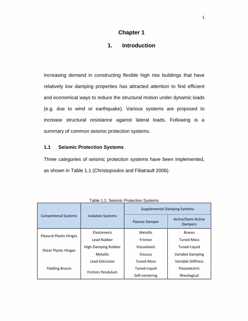
1.1 Seismic Protection Systems
Three categories of seismic protection systems have been implemented,
as shown in Table 1.1 (Christopoulos and Filiatrault 2006).
Table 1.1: Seismic Protection Systems
Conventional Systems Isolation Systems
Supplemental Damping Systems
Passive Damper Active/Semi-Active Dampers
Flexural Plastic Hinges Elastomeric Metallic Braces
Lead Rubber Friction Tuned-Mass
Shear Plastic Hinges High-Damping Rubber Viscoelastic Tuned-Liquid
Metallic Viscous Variable Damping
Yielding Braces
Lead-Extrusion Tuned-Mass Variable Stiffness
Friction Pendulum Tuned-Liquid Piezoelectric
Self-centering Rheological
2
1.1.1 Conventional Systems
These systems are based on traditional concepts and use stable inelastic
hysteresis to dissipate energy. This mechanism can be reached by plastic
hinging of columns, beams or walls, during axial behaviour of brace
elements by yielding in tension or buckling in compression or through
shear hinging of steel members.
1.1.2 Isolation Systems
Isolation systems are usually employed between the foundation and base
elements of the buildings and between the deck and the piers of bridges.
These systems are designed to have less amount of lateral stiffness
relative to the main structure in order to absorb more of the earthquake
energy. A supplemental damping system could be attached to the isolation
system to reduce the displacement of the isolated structure as a whole.
1.1.3 Supplemental Damping Systems
Supplemental damping system can be categorized in three groups as
passive, active and semi-active systems. These dampers are activated by
the movement of structure and decrease the structural displacements by
dissipating energy via different mechanisms.
1.1.3.1 Active Systems. Active systems monitor the structural behaviour,
and after processing the information, in a short time, generate a set of
forces to modify the current state of the structure. Generally, an active
control system is made of three components: a monitoring system that is
3
able to perceive the state of the structure and record the data using an
electronic data acquisition system; a control system that decides the
reaction forces to be applied to the structure based on the output data
from monitoring system and; an actuating system that applies the physical
forces to the structure. To accomplish all these, an active control system
needs continuous external power source. The loss of power that might be
experienced during a catastrophic event may render these systems
ineffective.
1.1.3.2 Semi-Active Systems. Semi-active systems are similar to active
systems except that compared to active ones they need less amount of
external power. Instead of exerting additional forces to the structural
systems, semi-active systems control the vibrations by modifying
structural properties (for example damping modification by controlling the
geometry of orifices in a fluid damper). The need for external power
source has also limited the application of semi-active systems.
1.1.3.3 Passive Mechanism. Passive systems dissipate part of the
structural seismic input energy without any need for external power
source. Their properties are constant during the seismic motion of the
structure and cannot be modified. Passive control devices have been
shown to work efficiently; they are robust and cost-effective. As such, they
are widely used in civil engineering structures. The main categories of the
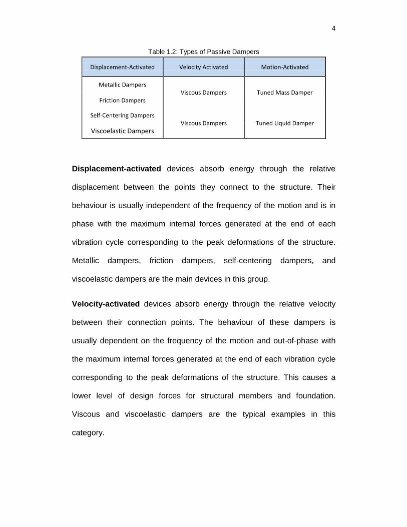
passive energy dissipation systems can be seen in Table 1.2
(Christopoulos and Filiatrault 2006).
4
Table 1.2: Types of Passive Dampers
Displacement-Activated Velocity Activated Motion-Activated
Metallic Dampers Viscous Dampers Tuned Mass Damper
Friction Dampers
Self-Centering Dampers Viscous Dampers Tuned Liquid Damper
Viscoelastic Dampers
Displacement-activated devices absorb energy through the relative
displacement between the points they connect to the structure. Their
behaviour is usually independent of the frequency of the motion and is in
phase with the maximum internal forces generated at the end of each
vibration cycle corresponding to the peak deformations of the structure.
Metallic dampers, friction dampers, self-centering dampers, and
viscoelastic dampers are the main devices in this group.
Velocity-activated devices absorb energy through the relative velocity
between their connection points. The behaviour of these dampers is
usually dependent on the frequency of the motion and out-of-phase with
the maximum internal forces generated at the end of each vibration cycle
corresponding to the peak deformations of the structure. This causes a
lower level of design forces for structural members and foundation.
Viscous and viscoelastic dampers are the typical examples in this
category.
5
Motion-activated dampers are secondary devices that absorb structural
energy through their motion. They are tuned to resonate with the main
structure, but, out-of-phase from it. These dampers absorb the input
energy of the structure and dissipate it by introducing extra forces to the
structure; therefore, they let less amount of energy to be experienced by
the structure. Tuned mass dampers (TMDs) and tuned liquid dampers
(TLDs) are the examples in this category.
1.2 Tuned Liquid Damper
1.2.1 History
Since 1950s liquid dampers have been used to stabilize marine vessels or
to control wobbling motion of satellites. In the late 1970s TLD has started
to be used in civil engineering to reduce structural motion; Vandiver and
Mitome (1979) used TLD to reduce the wind vibration of a platform. Also,
Mei (1978) and Yamamoto et al. (1982) looked into structure-wave
interactions using numerical methods. In the early 1980s important
parameters such as liquid height, mass, frequency, and damping for a
TLD attached to offshore platforms were studied by Lee and Reddy
(1982). Bauer (1984) introduced a rectangular tank full of two immiscible
liquids to a building structure. Kareem and Sun (1987), Sato (1987),
Toshiyuki and Tanaka, and Modi and Welt (1987) were among the first
researchers who suggested using TLD in civil structures.
6
Tuned liquid dampers (TLDs) can be implemented as an active or passive
device and are divided into two main categories: tuned sloshing dampers
(TSD) and tuned liquid column dampers (TLCDs).
1.2.2 Tuned Liquid Column Dampers
Tuned liquid column dampers (TLCD) combine the effect of liquid motion
in a tube, which results in a restoring force using the gravity effect of the
liquid, and the damping effect caused by loss of hydraulic pressure (Sakai
et al. 1989).
Some advantages of TLCD are: (i) it can have any arbitrary shape which
helps it to be fitted in an existing structure; (ii) its behaviour is quite well
understood; (iii) the TLCD damping can be controlled by adjusting the
orifice opening; (iv) the TLCD frequency can be modified by adjusting the
liquid column in the tube. A Double Tuned Liquid Column Damper
(DTLCD) is made of two TLCDs in two directions of motion (Kim et al.
2006).Thereby DTLCD acts in more than one direction eliminating the
limitation of regular unidirectional TLDC.
1.2.3 Tuned Sloshing Damper
A tuned sloshing damper (TSD) dissipates energy through the liquid
boundary layer friction, the free surface contamination, and wave breaking
(due to the horizontal component of the liquid velocity related to the wave
motion, wave crests descend as the amplitude increases; at this point
simple linear models are not able to describe the liquid behaviour). A TSD
7
can act as a shallow or deep water damper. It is considered that waves in
the range of ½>h/L>1/20 to 1/25 are shallow water waves, where h is
water depth and L is wave length (Sun et al. 1992). Recent studies
(Banerji et al. 2000; Seto 1996) show that a ratio equal to or less than 0.15
introduces more amount of damping corresponding to more energy
dissipation. Under high amplitude excitations, shallow water TSDs
dissipate a large amount of energy due to its nonlinear behaviour
corresponding to wave breaking (Sun et al. 1992). On another hand, a
linear behaviour can be observed for the deep water case even under high
excitations (Kim et al. 2006).
The liquid frequency plays an important role in the TLD behaviour. Earlier
experimental studies (Sun et al. 1992) have shown that the optimum value
of the liquid frequency is a value near the excitation frequency where the
liquid is in resonance with the tank motion. Therefore, tuning the TLD
frequency to the natural frequency of the structure will provide significant
amount of energy dissipation. Mass ratio (the ratio of the mass of water to
that of the whole structural levels) is another significant parameter that
affects the behavior of TLD-structure system. It is shown that with a
relatively small mass ratio (e.g. 4%), without contributing significantly to
the overall inertia of the system, effective structural response reduction
can be obtained (Banerji et al. 2000).
In comparison with other passive dampers TLD has some advantages
including: (i) Easy and cost-effective installation; (ii) Ease of tuning by
8
changing the liquid level or the tank dimensions; (iii) Ability to act as a
bidirectional damper; (iv) Effective even under small-amplitude vibrations
(Sun et al. 1992); (v) Can be used as the building water storage for fire
emergencies etc.
On the other hand, TLD has some issues such as: (i) Complex behavior
due to the highly non-linear sloshing motion of the liquid (ii) Damping
introduced by the liquid itself may not be enough for some applications. To
remedy this, screens (Tait 2008; Tait et al. 2007; Kaneko and Ishikawa
1999), effective tank shapes ( Deng and Tait 2009; Xin et al. 2009; Ueda
et al. 1992), and triangular sticks at the bottom of the tank (You et al.
2007) have been introduced to increase the damping. (iii) Inefficiency
during pulse-type ground motions (Xin et. Al 2009; Banerji et al. 2000),
when the water motion does not get a chance to dissipate enough energy;
(iv) The phenomenon of beating (Ikeda and Ibrahim 2005) where a
fraction of the energy absorbed by TLD returns back to the structure after
the excitation stops. A sloped bottom shape using density variable liquid
has been proposed to help solve the last two problems (Xin et al. 2009).
1.2.4 Active TLDs
TLDs have also been investigated as active/semiactive devices by
employing magnetic fluid (Abe et al. 1998; Wakahara et al. 1992), or
through use of propellers (Chen and Ko 2003).
9
1.2.5 TLDs in Practice
TLD has been employed in several civil engineering structures. The
Nagasaki Airport Tower (NAT) was the first TLD installation on an actual
ground structure in 1987 (Tamura et l 1995). In the other case, which is
quite similar to that of the NAT, a TLD was installed in June 1987 on
Yokohama Marine Tower (YMT) where the TLD is made of 39 cylindrical
multilayered vessels of acryl, with a height of 0.50 m and a diameter of
0.49 m (Tamura et l 1995). Another application of the TLD to a high-rise
hotel was the Shin Yokohama Prince (SYP) Hotel in Yokohama, where the
design parameters which affect the TLD behaviour were investigated
(Tamura et l 1995; Wakahara et al. 1992). Tuned Liquid Dampers have
also been implemented on bridges such as: Ikuchi Bridge and Sakitama
Bridges in Japan (Kaneko and Ishikawa 1999).
1.3 Scope of This Study and Outline of the Thesis
This study focuses on sloshing type of tuned liquid dampers. As
commonly done in the literature the abbreviation TLD is employed here for
this type of dampers and water is considered as the liquid inside the TLD.
To enable efficient use of TLDs in suppressing the structural vibrations
several models with different levels of complexity have been proposed in
the literature. On the other hand, in order to design an effective TLD, its
influential parameters such as frequency and mass must be tuned in a
way to significantly reduce the structural response. The main aim of this
10
study is to check the accuracy of selected models under different
conditions (i.e., different levels of excitation frequency, amplitude etc.) and
investigate the effect of selected TLD parameters that affect their
response using real-time hybrid pseudo-dynamic testing method.
Chapters 1 and 2 provide background information and a through literature
review, respectively.
Various existing analytical models are considered in Chapter 3 and among
them three models are selected and explained in detail. The procedure of
implementation of the recommended models is also presented in this
chapter.
In Chapter 4 a series of real-time hybrid pseudo-dynamic tests are carried
out; and based on the test results, the accuracy of each selected model is
investigated. Also the effect of important TLD parameters on the response
reduction efficiency are explored.
Chapter 5 provides the summary and conclusions of this study.
Appendix A illustrates the procedure of solving the basic equations of
Sun’s Model.
Appendix B shows the MATLAB codes and Simulink model provided to
solve the suggested models in Chapter 3.
11
Chapter 2
2. Literature Review
Since the early 1980s TLD has been investigated by many researchers.
Lee et al. (1982) studied effective TLD parameters including liquid height,
mass, frequency, and damping for a TLD attached to offshore platforms.
Bauer (1984) was among the first researchers who applied TLDs to
ground civil engineering structures by introducing a rectangular tank full of
two immiscible liquids to decrease structural vibration. Wakahara et al.
(1992) and Tamamura et al. (1995) showed the effectiveness of TLDs
installed in real structures such as Nagasaki airport tower, Yokohama
Marine tower, and Shin Yokohama Prince (SYP) hotel to reduce the
structural vibration.
Shimizu and Hayama (1986) presented a numerical model to solve for
Navier-Stokes and continuity equation based on shallow water wave
theory. They descritized the main equations and solved them numerically.
Sun et al. (1992) suggested a nonlinear model that utilizes the shallow
water wave theory and solves Navier-Stokes and continuity equations
together. Furthermore, they introduced two empirical coefficients to
account for the effect of wave breaking which is a significant deficiency in
many other models. Modi and Seto (1997) also proposed a numerical
12
study considering non-linear behaviour of the TLD. It includes the effects
of wave dispersion as well as boundary-layers at the walls, floating particle
interactions at the free surface, and wave-breaking. However, the analysis
does not account for the impact dynamics of the wave striking the tank
wall. Furthermore, at lower liquid heights, corresponding to wave breaking
occurrence, the numerical analysis is not very accurate and a large
discrepancy exists between numerical and experimental results.
Sun et al. (1995) calibrated equivalent mass, stiffness, and damping of
TLD using a tuned mass damper (TMD) analogy from experimental data
of rectangular, circular, and annular tanks subjected to harmonic base
excitation.
Yu (1999) introduced a model based on an equivalent tuned mass damper
with non-linear stiffness and damping calculated from an energy matching
procedure. It is shown that the model is able to capture the TLD behaviour
under large amplitude excitations and during wave breaking.
Gardarsson et al. (2001) investigated the performance of a sloped-bottom
TLD with an angle of 30° to the tank base. It is shown that despite the
hardening spring behaviour of a rectangular TLD, the sloped-bottom one
behaves as a softening spring. Also, it is observed that more liquid mass
participates in sloshing force in the slopped-bottom case leading to more
energy dissipation.
13
Reed et al. (1998) investigated the TLD behaviour under large amplitude
excitations through experiments and compared the results with a
numerical model based on non-linear shallow water wave equations. It
was observed that the TLD frequency response increases as the
amplitude of excitation increases and TLD behaves as a hardening spring.
Also, it was captured that to achieve the most robust system, TLD
frequency should be tuned to a value less than structural response
frequency; so, the actual non-linear TLD frequency matches the structural
response.
Olson and Reed (2001) investigated the sloped-bottom TLDs using non-
linear stiffness and damping model developed by Yu (1999). The softening
spring behaviour of the sloped-bottom system was confirmed. Also, it is
concluded that the sloped-bottom tank should be tuned slightly higher than
the fundamental frequency of the structure to introduce the most effective
damping.
Xin et al. (2009) proposed a density variable TLD with sloping bottom and
experimentally investigated it on a ¼ -scale, three-story structure. The
density-variable control system had been observed to be more effective
and more robust than a corresponding flat bottom, plane water TLD in
decreasing story drift and floor acceleration of the structure.
Yamamoto and Kawahara (1999) used arbitrary Lagrangian-Eulerian
(ALE) form of Navier-Stokes equations to predict the liquid motion.
14
Improved-balancing-tensor-diffusivity and fractional–steps methods were
employed to discritize and solve the Navier-Stokes equations in space and
Newmark’s β method was used in time domain to predict the TLD-
structural interaction response. However the model did not verified with
experiments.
Siddique and Hamed (2005) presented a new numerical model to solve
Navier-Stokes and continuity equations. They mapped irregular, time-
dependent, unknown physical domain onto a rectangular computational
domain where the mapping function is unknown and is determined during
the solution. It is indicated that the algorithm can accurately predict the
sloshing motion of the liquid undergoing large interfacial deformations.
However, it is unable to predict the deformations in the case of surface
discontinuity such as existing of screens or when wave breaking occurs.
Kareem et al. (2009) presented a model for TLD using sloshing-slamming
(S2) analogy, which consist of a combination of the dynamic features of
liquid sloshing and slamming impact and is able to capture the behaviour
for both low and high amplitudes of excitations. However, experimental
results do not have a good agreement with the proposed model.
Li et al. (2002) solved continuity and momentum fluid equations for
shallow liquid using finite element method. They simplified the three-
dimensional problem into a one-dimensional problem that simplifies the
15
computation procedure. However the model was not verified with
experiments.
Frandsen (2005) developed a fully nonlinear 2-D σ-transformed finite
difference model based on inviscid flow equations in rectangular tanks.
Results were presented for small to steep non-breaking waves at a range
of tank depth to length ratios representing deep to near shallow water
cases. However, the model is not able to capture damping effects of liquid
and the shallow water wave behaviour.
Warnitchai and Pinkaew (1998) proposed a mathematical model of TLDs
that includes the non-linear effects of flow-dampening devices.
Experimental investigations with a wire mesh screen device were carried
out. With the introduction of the flow dampening device an increase in
sloshing damping and the non-linear characteristic of the damping was
observed; and the slight reduction in sloshing frequency agreed well with
the model predictions.
Kaneko and Ishikawa (1999) proposed an analytical model that is able to
account for the effect of submerged nets on the TLD behaviour based on
shallow water wave theory. It is shown that the optimal damping factor can
be achieved by nets and the structural vibration will reduce more in
presence of nets.
Tait (2008) developed an equivalent linear mechanical model that
accounts for the energy dissipated by the damping screens for both
16
sinusoidal and random excitation. The model is validated using
experimental tests and a preliminary design procedure is suggested for a
TLD equipped with damping screens.
Cassolato et al. (2010) proposed inclined slat screens to increase the TLD
damping ratio. They calculated the pressure-loss coefficient for inclined
screens and estimated the energy dissipated by the screens. A model to
predict the fluid steady-state response was also developed. It was
observed that a TLD equipped with adjustable inclined screens could
introduce a constant damping ratio over a range of excitation amplitudes.
It was also captured that increasing the screen angle decreases the TLD
damping ratio.
Li and Wang (2004) suggested multiple TLDs to reduce multi-modal
responses of tall buildings and high-rise structures to earthquake ground
motion excitations. TLDs were tuned to the first several natural periods of
structure. It was shown both theoretically and experimentally that having
the same mass as a single TLD, multi-TLDs are more effective to reduce
structural motion up to 40%. Koh et al. (1995) also investigated multiple
liquid dampers tuned to several modal frequencies of the structure. It was
shown that multiple TLDs provide a better vibration control than TLDs
tuned to a particular modal frequency. Furthermore, they captured the
TLD dependency on the nature of excitation and the significant effect of
the TLD’s position on the vibration response.
17
Tait et al. (2005, 2007) conducted a study on 2D TLDs behaviour. They
subjected the TLD to both 1D and 2D horizontal excitations. The sloshing
response of the water in the tank was characterized by the free surface
motion, the resulting base shear force, and evaluation of the energy
dissipated by the sloshing water. Results showed a decoupled behaviour
for the 2D TLD which allows rectangular tanks to be used as 2D TLDs and
simultaneously reduce the dynamic response of a structure in two
perpendicular modes of vibration.
Tait and Deng (2009) introduced models of triangular-bottom, sloped-
bottom, parabolic-bottom, and flat-bottom tanks using the linear long wave
theory. The energy dissipated by damping screens and the equivalent
mechanical properties including effective mass, natural frequency, and
damping ratio of the TLDs were compared for different tank geometries. It
was shown that the normalized effective mass ratio (the liquid mass that
participates in sloshing) for a parabolic-bottom tank and a sloped-bottom
tank with a sloping angle of 20 deg are larger than the normalized
effective mass ratio of triangular-bottom and flat-bottom tanks. Idir et al.
(2009) derived the natural frequency of the water sloshing wave for
various tank bottom shapes from the equivalent flat bottom tank using the
linear wave theory. The frequency formula was shown to be accurate at
weak excitations, particularly for V and arc bottom-shaped tanks.
Banerji et al. (2000) studied the effectiveness of the important TLD
parameters based on the model introduced by Sun et al. (1992). The
18
optimum value of depth, mass and frequency ratios standing for the depth
of water to the length of tank, the mass of water to the mass of the
structure and the frequency of tank to the structural frequency were found
via experiments. Subsequently, a practical TLD design procedure is
suggested to control the seismic response of structures. Chang and Gu
(1999) conducted a theoretical and experimental study to achieve optimal
TLD properties installed on the top of a tall building and subjected to
vortex excitations (that is a special case of wind excitation). A series of
wind tunnel experiments corresponds to different TLD geometries were
performed. They proposed a TLD frequency ranges between 0.9 and 1.0
of that of the building model and a mass ratio of 2.3%.
Samanta and Banerjy (2010) theoritically modified TLD configuration
where the TLD rests on an elevated platform that is connected to the top
of the building through a rigid rod with a flexible rotational spring at its
bottom. Since for particular values of rotational spring flexibility the
rotational acceleration of the rod is in phase with the top structural
acceleration, the TLD was subjected to larger amplitude acceleration than
the traditional fixed bottom one and its efficiency was increased.
Modi and Akinturk (2002) focused on the installation of two-dimensional
wedge-shaped obstacles to amplify TLD energy dissipation efficiency. The
optimum obstacles’ geometry was determined through a parametric free
vibration study. It was shown that the damping factor can be increased by
approximately 19.8% in the optimum condition.
19
Abe et al. (1998) presented an active TLD which consists of magnetic fluid
activated by electromagnets. A rule-based control law of active dynamic
vibration absorbers was employed due to nonlinear behaviour of sloshing.
It was observed that active TLD is more effective to reduce structural
vibration and at the same time less sensitive to the error in tuning.
Ikeda (2010) investigated the influence of the two rectangular tanks
configuration on a two-storey structure response. In one case, one tank
was installed at the top and another at the second story, the second case
was putting one tank at the top and the last one was installing both tanks
at the top. He concluded that multiple tanks are less effective in reducing
structural response.
Ikeda (2003) investigated the TLD nonlinear behaviour attached to a linear
structure subjected to a vertical harmonic excitation. He observed that by
selecting an optimal liquid level, a liquid tank can be used as a damper to
suppress vertical sinusoidal excitations.
Ikeda and Ibrahim (2005) studied the nonlinear random interaction of an
elastic structure with liquid sloshing dynamics in a cylindrical tank
subjected to a vertical narrow-band random excitation. Four regimes of
liquid surface motion were observed and uni-modal sloshing modeling
found to reasonably investigate the structure-TLD interaction. Biswall et al.
(2003, 2004) investigated the effects of annular baffles on cylindrical TLD
20
behaviour. It was captured that the sloshing frequencies of liquid in the
flexible-tank–baffle system are lower than those of the rigid system.
Tait et al. (2005) performed a range of experimental studies to investigate
the TLD behaviour in terms of the free surface motion, the resulting base
shear forces, and the energy dissipated by a TLD with slat screens based
on a linear (Fediw et al. 1995) and non-linear (kaneko and Ishikawa 1999)
model. It is observed that the non-linear model is able to accurately
describe the response while the linear model is an appropriate tool for an
initial estimate of the energy dissipating characteristics of a TLD.
Furthermore, larger liquid depth to tank length values and using multiple
screens had been investigated based on experimental results. Also, a
method is presented to determine the loss coefficient of screens.
Lieping et al. (2008) suggested using Distributed tuned liquid dampers
(DTLDs) to fill the empty space inside the pipes or boxes of cast-in-situ
hollow reinforced concrete (RC) floor slabs to increase structural damping
ratio.
Lee et al. (2007) performed a real-time hybrid pseudodynamic (PSD) test
to evaluate the TLD performance. In this method the structure was
modeled in a computer and the tank was tested physically. They
compared results with the conventional shaking table test and indicated
that the performance of the TLD can be accurately evaluated using the
21
real-time hybrid shaking table testing method RHSTTM without the
physical structural model.
22
Chapter 3
3. Analytical Models
In this chapter selected models that are considered in this study are
introduced. Since the liquid behaviour is highly nonlinear, considering
nonlinearity is of crucial importance. Also, using shallow water in tanks
leads to the wave breaking occurrence under various excitation amplitude
and frequency combinations where the liquid surface is no longer
continuous. Therefore, the models presented in this chapter were selected
with the nonlinearity and wave breaking in mind for rectangular tanks filled
with water. Additionally, there are some researchers who considered
slopped bottom shape tanks (Olson and Reed 2001; Xin et al. 2009;
Gardarsson et al. 2001) and introduced models that are able to account
for slopped bottom shapes, one of these models is also included in this
study.
There are two common approaches that have been used to model the
liquid-tank behaviour. In the first one the dynamic equations of motion are
solved, whereas in the second approach the properties of the liquid
damper are presented by equivalent mass, stiffness and damping ratio
essentially modeling the TLD as an equivalent TMD (Tuned Mass
Damper).
23
3.1 Solving Liquid Equations of Motion
Several researchers have investigated the liquid behaviour based on
solving the liquid equations of motion. The assumptions they made along
with numerical methods they used to solve the liquid equations of motion
have a significant effect on their prediction. Ohyama and Fujji (1989) were
among the first who introduced a numerical model for the TLD. Using
potential flow theory their model was able to take care of nonlinearity;
however, computational time was the main problem with this model (Sun
et al. 1992). Kaneko and Ishikawa (1999) used an integrating scheme to
solve continuity and Navier-Stokes equations without any consideration for
wave breaking. Zang et al. (2000) used a linearized form of Navier-Stokes
equations. Fediew et al. (1995) assumed that the derivative and higher
orders of the velocity and wave height can be neglected due to small
values of velocity and wave height; however, this assumption works for
weak excitations or when the frequency of excitation is away from that of
the TLD (Lepelletier and Raichlen 1988). Ramaswamy et al. (1986) solved
nonlinear Navier-Stokes equations using Lagrangian description of fluid
motion and finite element method. The model has some physical problems
involving sloshing dynamics of inviscid and viscous fluids. Although the
model is based on nonlinear equations, but, considering only small
amplitude excitations, they assumed a linear behaviour of the liquid
sloshing. Yamamoto and Kawahara (1999) used arbitrary Lagrangian-
Eulerian (ALE) form of Navier-Stokes equations to predict the liquid
24
motion. The model tends to be unstable in the case of large amplitude
sloshing. To solve the instability problem a smoothing factor is considered
and the accuracy is highly dependent to the value of this factor that varies
from zero to one with no clear outline for the selection. Siddique and
Hamed (2005) presented a new numerical model to solve Navier-Stokes
and continuity equations. Although it is indicated that the algorithm can
accurately predict the sloshing motion of the liquid under large excitations,
the model is unable to predict the deformations in the case of surface
discontinuity where screen exist or wave breaking occurs. Frandsen
(2005) developed a fully nonlinear 2-D σ-transformed finite difference
model based on inviscid flow equations in rectangular tanks. The model
was not able to capture damping effects of liquid and shallow water wave
behaviour.
3.1.1 Sun’s Model
Sun et al. (1992) introduced a model to solve nonlinear Navier-Stokes and
continuity equations. A combination of boundary layer theory and shallow
water wave theory is employed and resulting equations were solved using
numerical methods. An important aspect of this model is that it considers
wave breaking under large excitations by means of two emprical
coefficients. In what follows, a summary of this model will be provided.
The rigid rectangular tank shown in figure 3.1 with the length 2𝑎𝑎, width 𝑏𝑏
and the undisturbed water level ℎ is subjected to a lateral displacement 𝑥𝑥𝑠𝑠.
The liquid motion is assumed to develop only in the 𝑥𝑥 − 𝑧𝑧 plane. It is also
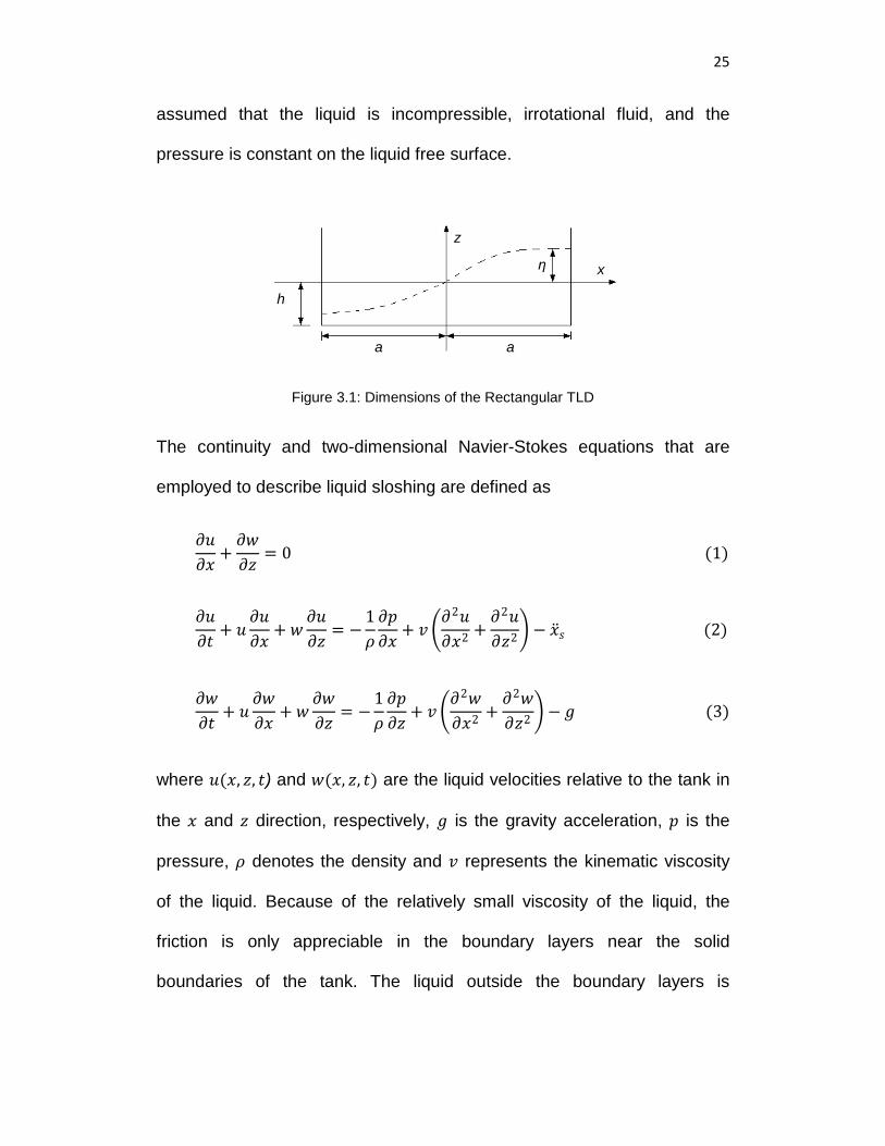
25
assumed that the liquid is incompressible, irrotational fluid, and the
pressure is constant on the liquid free surface.
Figure 3.1: Dimensions of the Rectangular TLD
The continuity and two-dimensional Navier-Stokes equations that are
employed to describe liquid sloshing are defined as
𝜕𝜕𝜕𝜕𝜕𝜕𝑥𝑥
+𝜕𝜕𝜕𝜕𝜕𝜕𝑧𝑧
= 0 (1)
𝜕𝜕𝜕𝜕𝜕𝜕𝜕𝜕
+ 𝜕𝜕𝜕𝜕𝜕𝜕𝜕𝜕𝑥𝑥
+ 𝜕𝜕𝜕𝜕𝜕𝜕𝜕𝜕𝑧𝑧
= −1𝜌𝜌𝜕𝜕𝑝𝑝𝜕𝜕𝑥𝑥
+ 𝑣𝑣 �𝜕𝜕2𝜕𝜕𝜕𝜕𝑥𝑥2 +
𝜕𝜕2𝜕𝜕𝜕𝜕𝑧𝑧2� − ��𝑥𝑠𝑠 (2)
𝜕𝜕𝜕𝜕𝜕𝜕𝜕𝜕
+ 𝜕𝜕𝜕𝜕𝜕𝜕𝜕𝜕𝑥𝑥
+ 𝜕𝜕𝜕𝜕𝜕𝜕𝜕𝜕𝑧𝑧
= −1𝜌𝜌𝜕𝜕𝑝𝑝𝜕𝜕𝑧𝑧
+ 𝑣𝑣 �𝜕𝜕2𝜕𝜕𝜕𝜕𝑥𝑥2 +
𝜕𝜕2𝜕𝜕𝜕𝜕𝑧𝑧2 � − 𝑔𝑔 (3)
where 𝜕𝜕(𝑥𝑥, 𝑧𝑧, 𝜕𝜕) and 𝜕𝜕(𝑥𝑥, 𝑧𝑧, 𝜕𝜕) are the liquid velocities relative to the tank in
the 𝑥𝑥 and 𝑧𝑧 direction, respectively, 𝑔𝑔 is the gravity acceleration, 𝑝𝑝 is the
pressure, 𝜌𝜌 denotes the density and 𝑣𝑣 represents the kinematic viscosity
of the liquid. Because of the relatively small viscosity of the liquid, the
friction is only appreciable in the boundary layers near the solid
boundaries of the tank. The liquid outside the boundary layers is
h
x η
a a
z
26
considered as potential flow and the velocity potential can be expressed
as (Sun 1991)
𝛷𝛷(𝑥𝑥, 𝑧𝑧, 𝜕𝜕) = −𝑔𝑔𝑔𝑔2𝜔𝜔
cosh�𝑘𝑘(ℎ + 𝑧𝑧)�cosh(𝑘𝑘ℎ) cos(𝑘𝑘𝑥𝑥 − 𝜔𝜔𝜕𝜕) (4 − 1)
where 𝑘𝑘 is wave number and H is defined as (Sun 1991)
𝑔𝑔 =2𝜂𝜂
sin(𝑘𝑘𝑥𝑥 − 𝜔𝜔𝜕𝜕) (4 − 2)
Based on the shallow water wave theory, potential 𝛷𝛷 is assumed as
(Shimisu and Hayama 1986)
𝛷𝛷(𝑥𝑥, 𝑧𝑧, 𝜕𝜕) = ��𝛷(𝑥𝑥, 𝜕𝜕). cosh�𝑘𝑘(ℎ + 𝑧𝑧)� (4 − 3)
The boundary conditions are described as
𝜕𝜕 = 0 on the end walls (𝑥𝑥 = ±𝑎𝑎); 𝜕𝜕 = 0 on the bottom (𝑧𝑧 = −ℎ); 𝜕𝜕 = 𝜕𝜕𝜂𝜂𝜕𝜕𝜕𝜕
+
𝜕𝜕 𝜕𝜕𝜂𝜂𝜕𝜕𝑥𝑥
on the free surface (𝑧𝑧 = ℎ); and 𝑝𝑝 = 𝑝𝑝0 = constant on the free surface
(𝑧𝑧 = ℎ)
where 𝜂𝜂(𝑥𝑥, 𝜕𝜕) is the free surface elevation.
��𝛷(𝑥𝑥, 𝜕𝜕) in equation (4-3) can be determined by the boundary conditions.
Then, using equation (4-3), 𝜕𝜕 and its differentials are expressed in terms
of 𝜕𝜕. Since the liquid depth is shallow, the governing equations are
integrated with respect to z from bottom to free surface to obtain:
27
𝜕𝜕𝜂𝜂𝜕𝜕𝜕𝜕
+ ℎσ𝜕𝜕(𝜙𝜙𝜕𝜕)𝜕𝜕𝑥𝑥
= 0 (5)
𝜕𝜕𝜕𝜕𝜕𝜕𝜕𝜕
+ �1 − 𝑇𝑇𝑔𝑔2�𝜕𝜕𝜕𝜕𝜕𝜕𝜕𝜕𝑥𝑥
+ 𝐶𝐶𝑓𝑓𝑓𝑓 2𝑔𝑔𝜕𝜕𝜂𝜂𝜕𝜕𝑥𝑥
+ 𝑔𝑔ℎ𝜎𝜎𝜙𝜙𝜕𝜕2𝜂𝜂𝜕𝜕𝑥𝑥2
𝜕𝜕𝜂𝜂𝜕𝜕𝑥𝑥
= −𝐶𝐶𝑑𝑑𝑎𝑎𝜆𝜆𝜕𝜕 − ��𝑥𝑠𝑠 (6)
Where 𝜎𝜎 = tanh(𝑘𝑘ℎ) /𝑘𝑘ℎ,𝜙𝜙 = tanh�𝑘𝑘(ℎ + 𝜂𝜂)� /tanh(𝑘𝑘ℎ),𝑇𝑇𝑔𝑔 = tanh(𝑘𝑘(ℎ +
𝜂𝜂)), 𝜕𝜕 and 𝜂𝜂 are the independent variables of these equations. 𝜆𝜆 in
equation (6) is a damping coefficient accounting for the effects of bottom,
side wall and free surface, and is determined as (Sun et al. 1989):
𝜆𝜆 =1
(𝜂𝜂 + ℎ)8
3𝜋𝜋�𝜔𝜔𝑙𝑙𝑣𝑣 �1 + �
2ℎ𝑏𝑏� + 𝑆𝑆� (7)
In which S stands for a surface contaminating factor and a value of one
corresponding to fully contaminated surface is used in this model (Sun et.
Al 1992). 𝜔𝜔𝑙𝑙 is the fundamental linear sloshing frequency of the liquid and
can be found as (Sun 1991)
𝜔𝜔𝑙𝑙 = �𝜋𝜋𝑔𝑔2𝑎𝑎
tanh �𝜋𝜋ℎ2𝑎𝑎� (8)
𝐶𝐶𝑓𝑓𝑓𝑓 and 𝐶𝐶𝑑𝑑𝑎𝑎 in equation (6) are employed to account for wave breaking
when (𝜂𝜂 > ℎ). These coefficients are initially equal to a unit value, and
when wave breaking occurs, 𝐶𝐶𝑓𝑓𝑓𝑓 takes a constant value equal to 1.05 as
suggested by Sun et al. (1992). 𝐶𝐶𝑑𝑑𝑎𝑎 depends on 𝑥𝑥𝑠𝑠 𝑚𝑚𝑎𝑎𝑥𝑥 that is the
maximum displacement experienced by the structure at the location of the
TLD, when there is no TLD attached; and it can be found as
𝐶𝐶𝑑𝑑𝑎𝑎 = 0.57�ℎ2𝜕𝜕𝑙𝑙
2𝑎𝑎𝑥𝑥𝑠𝑠 𝑚𝑚𝑎𝑎𝑥𝑥 (9)
28
Equations (5) and (6) are discretized in space by finite difference method
and solved simultaneously using Runge-Kutta-Gill method to find u and η.
Knowing η the force introduced at the walls of the TLD can be described
as [29]:
𝐹𝐹 =𝜌𝜌𝑔𝑔𝑏𝑏
2[(𝜂𝜂𝑛𝑛 + ℎ)2 − (𝜂𝜂0 + ℎ)2] (10)
where 𝜂𝜂𝑛𝑛 and 𝜂𝜂0 are the free surface elevations at the right and left tank
walls, respectively.
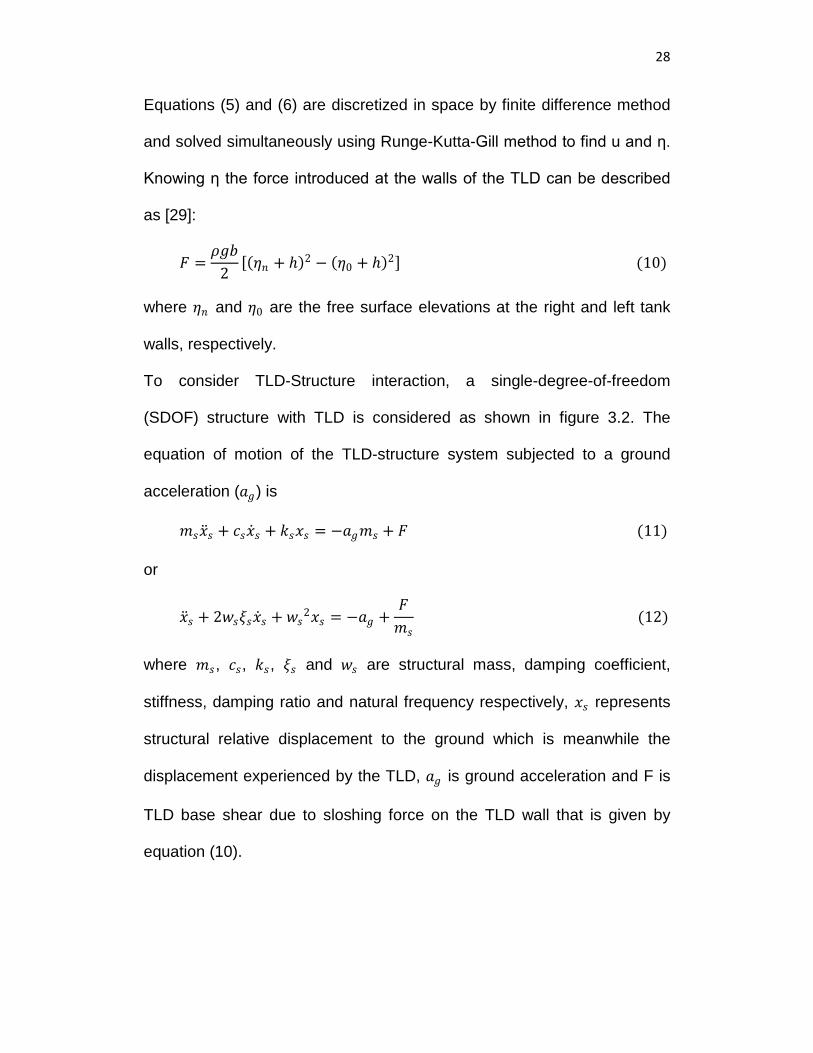
To consider TLD-Structure interaction, a single-degree-of-freedom
(SDOF) structure with TLD is considered as shown in figure 3.2. The
equation of motion of the TLD-structure system subjected to a ground
acceleration (𝑎𝑎𝑔𝑔) is
𝑚𝑚𝑠𝑠��𝑥𝑠𝑠 + 𝑐𝑐𝑠𝑠��𝑥𝑠𝑠 + 𝑘𝑘𝑠𝑠𝑥𝑥𝑠𝑠 = −𝑎𝑎𝑔𝑔𝑚𝑚𝑠𝑠 + 𝐹𝐹 (11)
or
��𝑥𝑠𝑠 + 2𝜕𝜕𝑠𝑠𝜉𝜉𝑠𝑠��𝑥𝑠𝑠 + 𝜕𝜕𝑠𝑠2𝑥𝑥𝑠𝑠 = −𝑎𝑎𝑔𝑔 +𝐹𝐹𝑚𝑚𝑠𝑠
(12)
where 𝑚𝑚𝑠𝑠, 𝑐𝑐𝑠𝑠, 𝑘𝑘𝑠𝑠, 𝜉𝜉𝑠𝑠 and 𝜕𝜕𝑠𝑠 are structural mass, damping coefficient,
stiffness, damping ratio and natural frequency respectively, 𝑥𝑥𝑠𝑠 represents
structural relative displacement to the ground which is meanwhile the
displacement experienced by the TLD, 𝑎𝑎𝑔𝑔 is ground acceleration and F is
TLD base shear due to sloshing force on the TLD wall that is given by
equation (10).
29
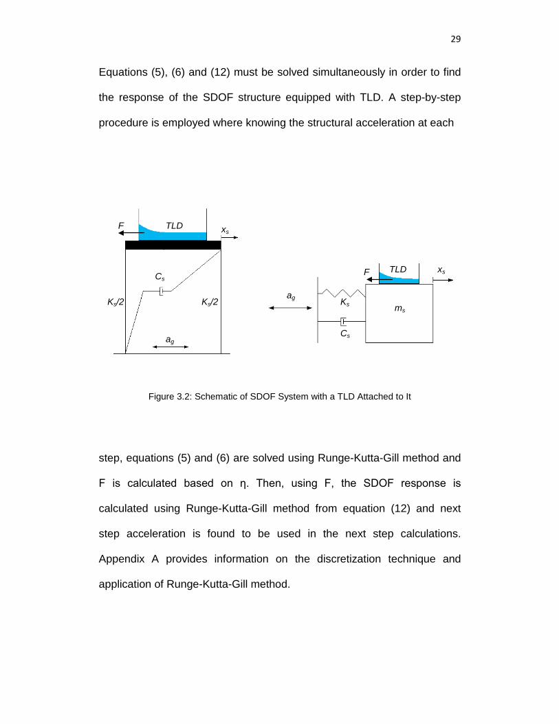
Equations (5), (6) and (12) must be solved simultaneously in order to find
the response of the SDOF structure equipped with TLD. A step-by-step
procedure is employed where knowing the structural acceleration at each
Figure 3.2: Schematic of SDOF System with a TLD Attached to It
step, equations (5) and (6) are solved using Runge-Kutta-Gill method and
F is calculated based on η. Then, using F, the SDOF response is
calculated using Runge-Kutta-Gill method from equation (12) and next
step acceleration is found to be used in the next step calculations.
Appendix A provides information on the discretization technique and
application of Runge-Kutta-Gill method.
F TLD xs
ag
F TLD
Ks
Cs
ms
xs Cs
ms Ks/2 Ks/2
ag
30
3.2 Equivalent TMD Models
Another approach to investigate TLD behaviour is replacing the TLD by its
equivalent TMD and finding the effective TMD properties such as stiffness,
damping ratio, and mass that can properly describe TLD characteristics.
These equivalent properties are found through experimental procedures.
Sun et al. (1995) found equivalent TMD properties base on nonlinear
Navier-Stokes equations and shallow water wave theory. However,
theexperimental cases presented in this study are limited. Casciati et al.
(2003) proposed a linear model which can interpret frustum-conical TLDs
behaviour for small excitations. The model is not able to capture high
amplitude excitations and instability problems occur near resonance. Tait
(2008) developed an equivalent linear mechanical model that accounts for
the energy dissipated by the damping screens for both sinusoidal and
random excitation.
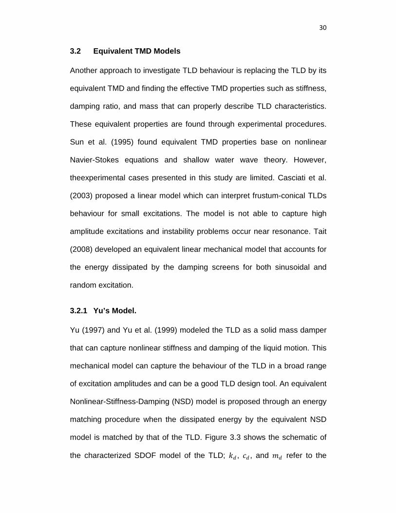
3.2.1 Yu’s Model.
Yu (1997) and Yu et al. (1999) modeled the TLD as a solid mass damper
that can capture nonlinear stiffness and damping of the liquid motion. This
mechanical model can capture the behaviour of the TLD in a broad range
of excitation amplitudes and can be a good TLD design tool. An equivalent
Nonlinear-Stiffness-Damping (NSD) model is proposed through an energy
matching procedure when the dissipated energy by the equivalent NSD
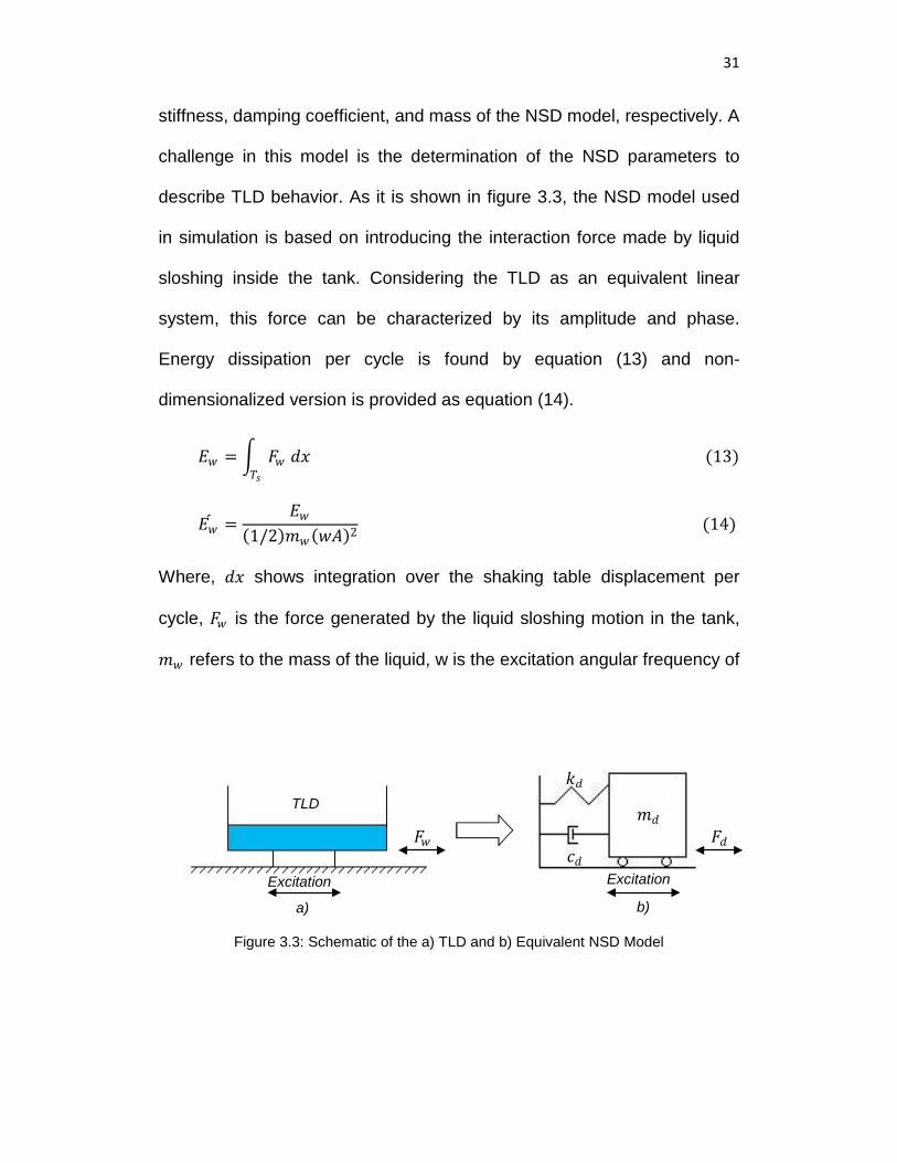
model is matched by that of the TLD. Figure 3.3 shows the schematic of
the characterized SDOF model of the TLD; 𝑘𝑘𝑑𝑑 , 𝑐𝑐𝑑𝑑 , and 𝑚𝑚𝑑𝑑 refer to the
31
stiffness, damping coefficient, and mass of the NSD model, respectively. A
challenge in this model is the determination of the NSD parameters to
describe TLD behavior. As it is shown in figure 3.3, the NSD model used
in simulation is based on introducing the interaction force made by liquid
sloshing inside the tank. Considering the TLD as an equivalent linear
system, this force can be characterized by its amplitude and phase.
Energy dissipation per cycle is found by equation (13) and non-
dimensionalized version is provided as equation (14).
𝐸𝐸𝜕𝜕 = � 𝐹𝐹𝜕𝜕 𝑑𝑑𝑥𝑥𝑇𝑇𝑠𝑠
(13)
𝐸𝐸��𝜕 =𝐸𝐸𝜕𝜕
(1/2)𝑚𝑚𝜕𝜕(𝜕𝜕𝑤𝑤)2 (14)
Where, 𝑑𝑑𝑥𝑥 shows integration over the shaking table displacement per
cycle, 𝐹𝐹𝜕𝜕 is the force generated by the liquid sloshing motion in the tank,
𝑚𝑚𝜕𝜕 refers to the mass of the liquid, w is the excitation angular frequency of
Figure 3.3: Schematic of the a) TLD and b) Equivalent NSD Model
Excitation
𝑐𝑐𝑑𝑑
𝑘𝑘𝑑𝑑
𝑚𝑚𝑑𝑑
𝐹𝐹𝑑𝑑
a)
𝐹𝐹𝜕𝜕
TLD
Excitation
b)
32
the shaking table (equation (8)), A is the amplitude of the sinusoidal
excitation and the denominator of (14) is the maximum kinetic energy of
the water mass treated as a solid mass.
Non-dimensional energy dissipation of the NSD model 𝐸𝐸��𝑑 is determined
based on NSD model behaviour when it is subjected to harmonic base
excitation with frequency ratio β. The non-dimensionalized amplitude ���𝐹𝑑𝑑�,
and phase 𝜙𝜙 that describe the interaction force of the NSD model and are
calculated as
���𝐹𝑑𝑑� =��1 + �4𝜉𝜉𝑑𝑑
2 − 1�𝛽𝛽2�2
+ 4𝜉𝜉𝑑𝑑2𝛽𝛽6
1 + �4𝜉𝜉𝑑𝑑2 − 2�𝛽𝛽2 + 𝛽𝛽4
(15)
𝜙𝜙 = 𝜕𝜕𝑎𝑎𝑛𝑛−1 �2𝜉𝜉𝑑𝑑𝛽𝛽3
−1 + �1 − 4𝜉𝜉𝑑𝑑2�𝛽𝛽2
� (16)
where 𝛽𝛽 = 𝑓𝑓𝑒𝑒 𝑓𝑓𝑑𝑑⁄ is the excitation frequency ratio, 𝑓𝑓𝑒𝑒 is the excitation
frequency, 𝑓𝑓𝑑𝑑 = (1/2π)�𝑘𝑘𝑑𝑑 𝑚𝑚𝑑𝑑⁄ is the natural frequency of the NSD,
𝜉𝜉𝑑𝑑 = 𝑐𝑐𝑑𝑑 𝑐𝑐𝑐𝑐𝑓𝑓⁄ is the damping ratio of the NSD model, 𝑐𝑐𝑐𝑐𝑓𝑓 = 2𝑚𝑚𝑑𝑑𝜕𝜕𝑑𝑑 is the
critical damping coefficient, 𝜕𝜕𝑑𝑑 = 2𝜋𝜋𝑓𝑓𝑑𝑑 is the linear fundamental natural
angular frequency, and 𝑚𝑚𝑑𝑑 , 𝑘𝑘𝑑𝑑 and 𝑐𝑐𝑑𝑑 are the mass, stiffness and
damping coefficients of the NSD model, respectively.
The non-dimensional energy dissipation of the NSD model at each
excitation frequency is defined as:
𝐸𝐸��𝑑 = 2𝜋𝜋���𝐹𝑑𝑑�𝑠𝑠𝑠𝑠𝑛𝑛𝜙𝜙 (17)
𝐸𝐸��𝑑 is fitted to 𝐸𝐸��𝜕 over high-frequency dissipation range of the frequency
using least-squares method. In this procedure 𝑚𝑚𝑑𝑑 = 𝑚𝑚𝜕𝜕 , and assuming
33
initial values for 𝜉𝜉𝑑𝑑 and 𝑓𝑓𝑑𝑑 , the stiffness and damping coefficients are
determined. The results are analyzed through two ratios; the first is
frequency shift ratio as defined by:
𝜉𝜉 =𝑓𝑓𝑑𝑑𝑓𝑓𝜕𝜕
(18)
where 𝑓𝑓𝜕𝜕 stands for the linear fundamental frequency of the liquid and is
defined as:
𝑓𝑓𝜕𝜕 =1
2𝜋𝜋�𝜋𝜋𝑔𝑔
2𝑎𝑎tanh �
𝜋𝜋ℎ2𝑎𝑎� (19)
where h is the undisturbed height of the water and a is the half length of
the tank. The second ratio is the stiffness hardening ratio 𝜅𝜅 that is defined
as
𝜅𝜅 =𝑘𝑘𝑑𝑑 𝑘𝑘𝜕𝜕
(20)
where 𝑘𝑘𝜕𝜕 = 𝑚𝑚𝜕𝜕(2𝜋𝜋𝑓𝑓𝜕𝜕)2
The above matching scheme is applied to a set of experimental tests in
order to evaluate the equivalent stiffness and damping ratio for the NSD
model. The equivalent stiffness and damping ratio are investigated as a
function of the wave height, water depth, amplitude of excitation and the
tank size. Non-dimensional value of the amplitude was found to be the
most suitable parameter to describe the stiffness and damping ratio. This
value is described as:
ᴧ =𝑤𝑤
2𝑎𝑎 (21)
34
where 𝑤𝑤 is the amplitude of excitation and a is the half length of the tank in
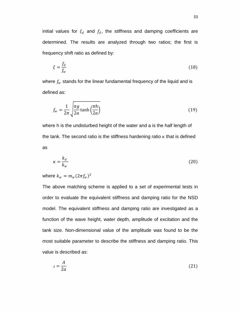
the direction of motion. To calculate 𝑤𝑤, as it is shown in figure 3.4, each
time the displacement curve crosses the time axis, the maximum
displacement during the previous half cycle xmax, i-1 is calculated and the
absolute value of that is considered as 𝑤𝑤 for the ith half cycle in order to
find ᴧ.
Figure 3.4: Displacement Time History to Calculate 𝑤𝑤
After finding the corresponding values of 𝜉𝜉 and κ from equations (18) and
(20), they are plotted versus ᴧ and the best-fitted curve is found in order to
find the equations for damping ratio and stiffness hardening ratio. Yu
(1997) and Yu et al. (1999) obtained the damping ratio as
𝜉𝜉𝑑𝑑 = 0.5 ᴧ0.35 (22)
As stiffness hardening ratio changes considerably before ᴧ = 0.03
(corresponding to weak wave breaking) and then starts to grow up sharply
after ᴧ = 0.03 (corresponding to strong wave breaking), Yu (1997) and Yu
et al. (1999) obtained the equation for 𝜅𝜅 is obtained as
x
time
i-1
Tank Displacement
xmax, i
xmax, i-1
i
35
𝜅𝜅 = 1.075 ᴧ0.007 ᴧ ≤ 0.03 weak wave breaking (23)
𝜅𝜅 = 2.52 ᴧ0.25 ᴧ ≤ 0.03 strong wave breaking (24)
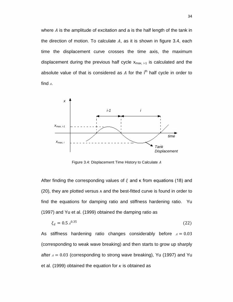
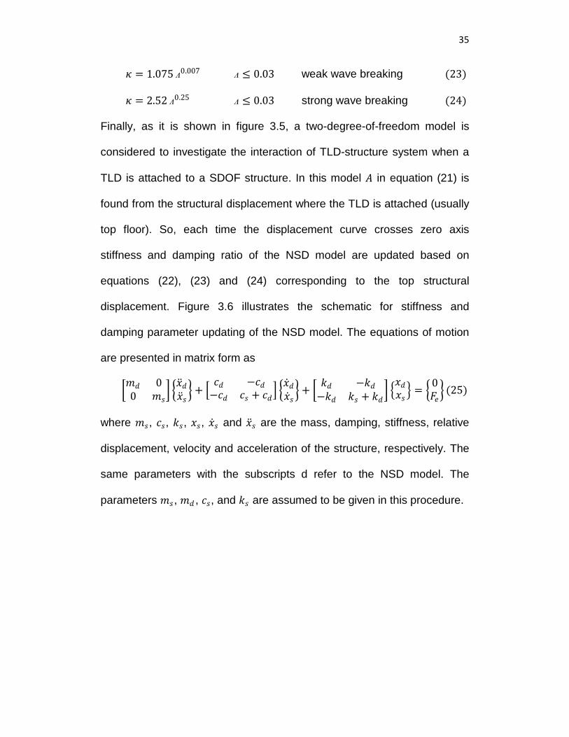
Finally, as it is shown in figure 3.5, a two-degree-of-freedom model is
considered to investigate the interaction of TLD-structure system when a
TLD is attached to a SDOF structure. In this model 𝑤𝑤 in equation (21) is
found from the structural displacement where the TLD is attached (usually
top floor). So, each time the displacement curve crosses zero axis
stiffness and damping ratio of the NSD model are updated based on
equations (22), (23) and (24) corresponding to the top structural
displacement. Figure 3.6 illustrates the schematic for stiffness and
damping parameter updating of the NSD model. The equations of motion
are presented in matrix form as
�𝑚𝑚𝑑𝑑 00 𝑚𝑚𝑠𝑠
� ���𝑥𝑑𝑑��𝑥𝑠𝑠� + �
𝑐𝑐𝑑𝑑 −𝑐𝑐𝑑𝑑−𝑐𝑐𝑑𝑑 𝑐𝑐𝑠𝑠 + 𝑐𝑐𝑑𝑑� �
��𝑥𝑑𝑑��𝑥𝑠𝑠� + � 𝑘𝑘𝑑𝑑 −𝑘𝑘𝑑𝑑
−𝑘𝑘𝑑𝑑 𝑘𝑘𝑠𝑠 + 𝑘𝑘𝑑𝑑� �𝑥𝑥𝑑𝑑𝑥𝑥𝑠𝑠 � = �0
𝐹𝐹𝑒𝑒� (25)
where 𝑚𝑚𝑠𝑠, 𝑐𝑐𝑠𝑠, 𝑘𝑘𝑠𝑠, 𝑥𝑥𝑠𝑠, ��𝑥𝑠𝑠 and ��𝑥𝑠𝑠 are the mass, damping, stiffness, relative
displacement, velocity and acceleration of the structure, respectively. The
same parameters with the subscripts d refer to the NSD model. The
parameters 𝑚𝑚𝑠𝑠, 𝑚𝑚𝑑𝑑 , 𝑐𝑐𝑠𝑠, and 𝑘𝑘𝑠𝑠 are assumed to be given in this procedure.
36
Figure 3.5: 2-DOF System: a) Structure with TLD b) Structure with NSD Model
Figure 3.6: Schematic for Determining the NSD Parameters
Given Constants: 𝑚𝑚𝑠𝑠 , 𝑘𝑘𝑠𝑠 , 𝑐𝑐𝑠𝑠 ,𝑚𝑚𝑑𝑑
Given Function: 𝐹𝐹𝑒𝑒
Initial Conditions: 𝑠𝑠 = 1, 𝑥𝑥𝑠𝑠 , 𝑥𝑥��𝑠
Get 𝐹𝐹𝑒𝑒 ,𝑠𝑠
𝑥𝑥𝑠𝑠
Equation (25)
Zero-Crossing
Yes
No
Calculate 𝑐𝑐𝑑𝑑 and 𝑘𝑘𝑑𝑑
Equations (22), (23) and (24)
Find 𝑤𝑤
End
Stop
Yes
No 𝑠𝑠 = 𝑠𝑠 + 1
a) b)
37
3.3 Sloped Bottom Models
There are studies on the effect of changing the tank bottom shape from
rectangular to sloped bottom pattern. Gardarsson et al. (2001)
investigated the performance of a sloped-bottom TLD with an angle of 30°
to the tank base. It is observed that more liquid mass participates in
sloshing force in the slopped-bottom case leading to more energy
dissipation. Olson and Reed (2001) investigated the sloped-bottom TLDs
using non-linear stiffness and damping model developed by Yu (1999). It
is shown that the sloped-bottom tank should be tuned slightly higher than
the fundamental frequency of the structure to introduce the most effective
damping. Tait and Deng (2009) showed that the normalized effective
mass ratio for a sloped-bottom tank with a sloping angle of 20° is larger
than the normalized effective mass ratio of flat-bottom tanks.
3.3.1 Xin’s Model
Xin (2006) and Xin et al. (2009) proposed a model that is capable to
investigate sloping-bottom TLD based on the linearized shallow water
wave equation (Gardarsson 1997), using the velocity potential function
and wave height equation suggested by Wang (1996) and liquid damping
introduced by Sun et al. (1995) and Sun (1991). As it is shown in figure
3.7, an equivalent flat-bottom TLD model is proposed to simulate the
sloping-bottom tank. The total contact area between water and the tank for
the sloped-bottom case and the equivalent flat-bottom tank is kept equal
(the length 𝐿𝐿′ of the equivalent flat-bottom tank is equal to the total length
38
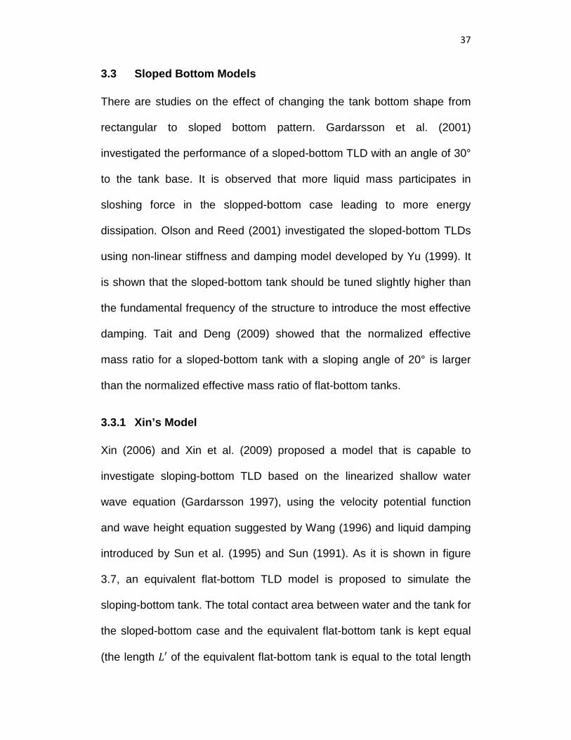
of the sloping bottom). The maximum water depth 𝑔𝑔′ remains the same
when the equivalent width of the flat-bottom tank 𝐵𝐵′ is decreased in order
to keep the total volume 𝑉𝑉𝜕𝜕 of the sloshing water the same as that of the
sloped-bottom tank. 𝐵𝐵′ is defined as (Xin 2006):
𝐵𝐵′ =𝑉𝑉𝜕𝜕𝑔𝑔′ 𝐿𝐿′
(26)
The horizontal control force 𝐹𝐹𝑗𝑗 (𝜕𝜕) applied to the 𝑗𝑗𝜕𝜕ℎ floor of the building
structure by a sloping-bottom TLD is equal to the resultant of the fluid
dynamic pressures on the left and right walls of the flat-bottom TLD tank;
and is expressed as (Xin et al. 2009)
𝐹𝐹𝑗𝑗 (𝜕𝜕) = −𝜌𝜌𝑉𝑉𝜕𝜕 ���𝑋𝑗𝑗 (𝜕𝜕) + ��𝑥𝑔𝑔(𝜕𝜕) + ��𝑦(𝜕𝜕)8𝐿𝐿′
𝜋𝜋3𝑔𝑔′ 𝜕𝜕𝑎𝑎𝑛𝑛ℎ𝜋𝜋𝑔𝑔′
𝐿𝐿′� (27)
Figure 3.7: Equivalent Flat-Bottom Tank
where 𝜌𝜌 is the water density, ��𝑋𝑗𝑗 (𝜕𝜕) represents the relative acceleration on
the 𝑗𝑗𝜕𝜕ℎ building floor with respect to the base of the building, ��𝑥𝑔𝑔(𝜕𝜕) refers to
the ground acceleration at the base of the building, and ��𝑦(𝜕𝜕) is the first
modal acceleration of water sloshing. The modal response of water
sloshing can be determined as
��𝑦(𝜕𝜕) + 2𝜉𝜉𝜕𝜕���𝑦(𝜕𝜕) + 𝜕𝜕� 2𝑦𝑦(𝜕𝜕) = −��𝑋𝑗𝑗 (𝜕𝜕) − ��𝑥𝑔𝑔(𝜕𝜕) (28)
𝑧𝑧
𝑥𝑥 𝑥𝑥
𝑧𝑧
𝐿𝐿′
𝑔𝑔′ = 𝑔𝑔𝑚𝑚𝑎𝑎𝑥𝑥
𝐿𝐿
𝑔𝑔𝑚𝑚𝑎𝑎𝑥𝑥
39
where
𝜉𝜉 =√2𝜕𝜕�𝑣𝑣 �1 + 2𝑔𝑔′
𝐵𝐵′ + 𝑆𝑆� 𝐿𝐿′
4𝜋𝜋𝑔𝑔′�𝑔𝑔𝑔𝑔′ (29)
and
𝜕𝜕� 2 =𝜋𝜋𝑔𝑔𝐿𝐿′
tanh�𝜋𝜋𝑔𝑔′
𝐿𝐿′� (30)
in which 𝑣𝑣 refers to the kinematic viscosity of the liquid and S (=1.0 )) is
the surface contamination factor ((Sun et. Al 1992)).
In order to consider TLD-structure interaction, the structural response to
the ground motion and force 𝐹𝐹𝑗𝑗 (𝜕𝜕) is written in the matrix form as
𝑀𝑀��𝑋 + 𝐶𝐶��𝑋 + 𝐾𝐾𝑋𝑋 = −𝑀𝑀𝑀𝑀��𝑥𝑔𝑔(𝜕𝜕) + 𝑀𝑀𝑓𝑓𝐹𝐹𝑗𝑗 (𝜕𝜕) (31)
Where M, C, and K are the mass, damping coefficient, and stiffness
matrices of the structure; ��𝑋, ��𝑋 , and 𝑋𝑋 represent the relative acceleration,
velocity, and displacement vectors with respect to the base of the building;
𝑀𝑀 is the earthquake influence vector with unity for all elements; and 𝑀𝑀𝑓𝑓 is
the TLD influence vector with zero elements except for the element
corresponding to the 𝑗𝑗𝜕𝜕ℎ floor of the building where the TLD is attached
that is unity.
Knowing the initial condition, equation (28) is solved and the tank
acceleration is calculated and used in equation (27) to find the interface
force. Having the interface force and using equation (31) structural
displacement and acceleration are found for next step calculations.
40
In this study, since the experiments were done for a rectangular tank,
these equations are solved for the equivalent rectangular tank in order to
investigate this model’s accuracy. The Simulink used to solve these
equations is presented in Appendix B.
41
Chapter 4
4. Experimental Results and Analysis
4.1 Testing Method
In this study the real-time hybrid Pseudodynamic (PSD) testing method
has been employed to investigate the TLD behaviour under a range of
structural parameters and load cases. Hybrid PSD testing method
combines computer simulation with physical by testing part of the structure
physically (experimental substructure) coupled with a numerical model of
the remainder of the structure (analytical substructure). When the
experimental substructure has load rate dependent vibration
characteristics as in the case of TLD, the hybrid PSD test needs to be
performed dynamically in real-time. By employing real-time hybrid PSD
test in this study, the structure-TLD interaction has been investigated by
only physically testing the TLD as the experimental substructure and a
wide range of TLD-structure system properties were easily investigated by
modifying the parameters of the structure as the analytical substructure.
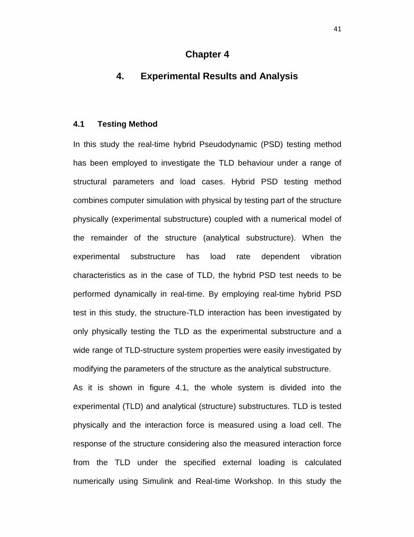
As it is shown in figure 4.1, the whole system is divided into the
experimental (TLD) and analytical (structure) substructures. TLD is tested
physically and the interaction force is measured using a load cell. The
response of the structure considering also the measured interaction force
from the TLD under the specified external loading is calculated
numerically using Simulink and Real-time Workshop. In this study the
42
analytical substructure is modeled as a single degree of freedom
oscillator. The displacement command generated by the Simulink model is
imposed on the shaker. The software/hardware communication and
synchronization issues are taken care of by using the WinCon/Simulink
interface.
Figure 4.1: Schematic of the Hybrid Testing Method
4.2 Test Setup
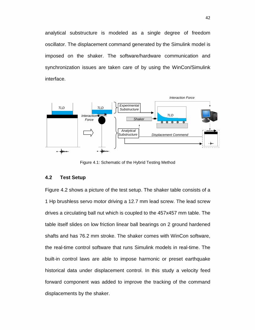
Figure 4.2 shows a picture of the test setup. The shaker table consists of a
1 Hp brushless servo motor driving a 12.7 mm lead screw. The lead screw
drives a circulating ball nut which is coupled to the 457x457 mm table. The
table itself slides on low friction linear ball bearings on 2 ground hardened
shafts and has 76.2 mm stroke. The shaker comes with WinCon software,
the real-time control software that runs Simulink models in real-time. The
built-in control laws are able to impose harmonic or preset earthquake
historical data under displacement control. In this study a velocity feed
forward component was added to improve the tracking of the command
displacements by the shaker.
Experimental Substructure
Analytical Substructure
Interaction Force
Displacement Commend
TLD
TLD TLD
Shaker Interaction
Force
43
The load cell is a 22.2 N (5 lb) load cell that can carry compression and
tension loads. The tank is made of plexi-glass that has dimensions of 464
mm (length), 305 mm (width). A water height of 40 mm which corresponds
to 0.667 Hz of sloshing frequency of the tank (based on equation (8)) was
selected there the weight of the TLD was 5.64 kg.
Figure 4.2: Experimental Setup
As it is shown in figures 4.1 and 4.2, the tank is placed on greased ball
bearings to eliminate friction. Special attention was given to keep the tank
in the perfectly horizontal position. Only a few degrees out of horizontal
position was observed to introduce large amount of error in the measured
44
restoring force. Two rollers are also placed at the two sides of the tank in
order to keep its movement in one direction.
4.3 TLD Subjected to Predefined Displacement History
This section summarizes the results where the TLD was subjected to
displacement histories with amplitude of 20 mm and various frequencies
to cover a range of β from 0.5 to 1.5. The frequency ratio β, as previously
defined, is the ratio of the frequency of loading to the sloshing frequency
of the tank. By considering the energy dissipated in each case (see figure
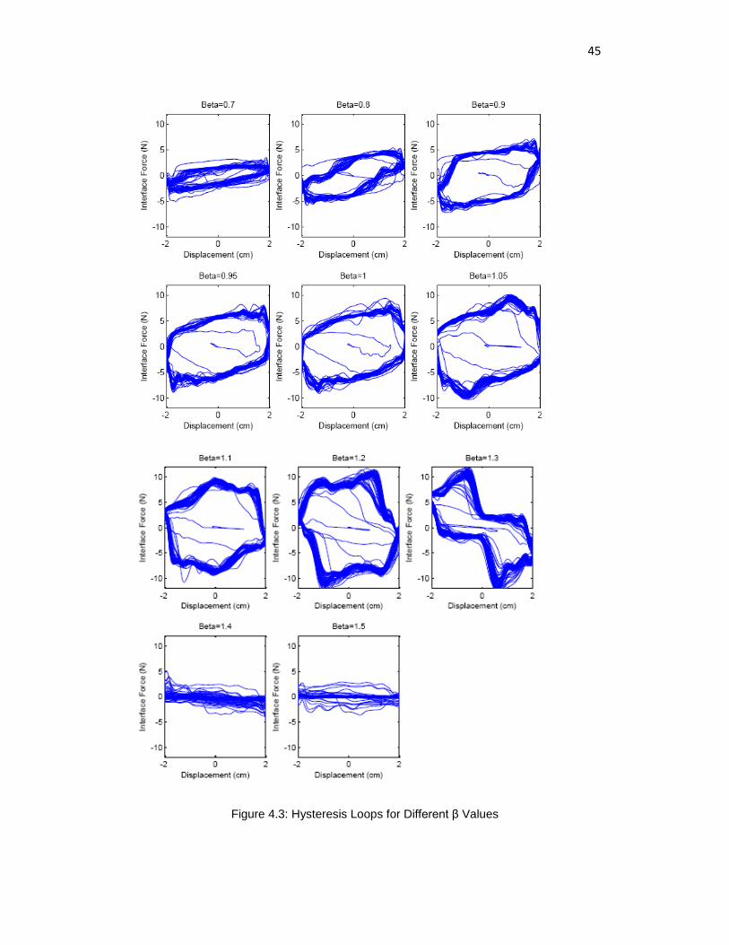
4.3), the effective value for β was obtained. As can be seen in figure 4.3
energy dissipated by the TLD increases until β<1.2, and starts to decrease
for values of β>1.2, rendering β=1.2 as the effective frequency in terms of
energy dissipation.
To shed some light into the TLD energy dissipation behavior, another set
of experiments were performed. In these tests, the water inside the TLD
was replaced with an equivalent solid mass while the TLD was imposed to
the same predefined displacement histories. The measured restoring
forces in these tests correspond to the inertia component of the interface
force. By subtracting the inertia component from the interface force, the
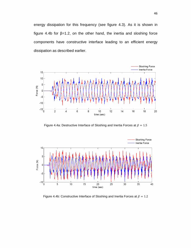
sloshing force was calculated for each frequency ratio. Figure 4.4a shows
the inertia and sloshing force components of the interface force for β=1.5.
It can be seen that these components have a destructive interface where
they almost cancel each other resulting in very little if not nonexistent
45
Figure 4.3: Hysteresis Loops for Different β Values
46
energy dissipation for this frequency (see figure 4.3). As it is shown in
figure 4.4b for β=1.2, on the other hand, the inertia and sloshing force
components have constructive interface leading to an efficient energy
dissipation as described earlier.
Figure 4.4a: Destructive Interface of Sloshing and Inertia Forces at 𝛽𝛽 = 1.5
Figure 4.4b: Constructive Interface of Sloshing and Inertia Forces at 𝛽𝛽 = 1.2
47
4.4 TLD-Structure Subjected to Sinusoidal Force
In this section, using real-time hybrid PSD method, the TLD-structure
system was investigated under a series of sinusoidal force. To be able to
observe weak and strong wave breaking behavior, three different force
amplitudes (i.e., 3 N, 5 N, and 8 N) were used while the forcing frequency
adjusted to be the same as the structural frequency (see table 4.1). In
addition to the forcing function amplitude, a range of structure to TLD
sloshing frequency ratio (α) from 0.5 to 1.5 was considered in the hybrid
simulations. The TLD properties were kept unchanged; to obtain the
aforementioned range of α, the structural stiffness in the analytical
substructure was adjusted. The mass of the structure and the structural
damping ratio remained unchanged (see table 4.1).
Table 4.1: Parameters for experiments introduced in Chapter 4.4
Structural Mass (m)
Structural Stiffness
(k)
Structural Damping
Coefficient (c)
Structural Damping Ratio (ξ)
Structural Frequency
(f)
Sinusoidal Force
Amplitude
Sinusoidal Force
Frequency
564 kg (1% Mass Ratio)
Adjusted to Change f
Adjusted to Keep ξ
Constant 0.20% Adjusted to
Change α 3N, 5N, and 8 N Equal to f
Structural displacements in the form of deformations relate to the damage
of the structural members during seismic events. On the other hand,
nonstructural components (ceiling- wall attachments, furniture etc) may
experience considerable inertial forces due to floor accelerations. Figure
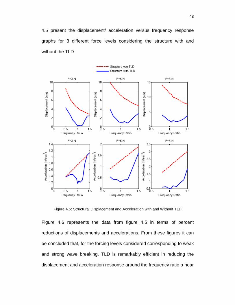
48
4.5 present the displacement/ acceleration versus frequency response
graphs for 3 different force levels considering the structure with and
without the TLD.
Figure 4.5: Structural Displacement and Acceleration with and Without TLD
Figure 4.6 represents the data from figure 4.5 in terms of percent
reductions of displacements and accelerations. From these figures it can
be concluded that, for the forcing levels considered corresponding to weak
and strong wave breaking, TLD is remarkably efficient in reducing the
displacement and acceleration response around the frequency ratio α near
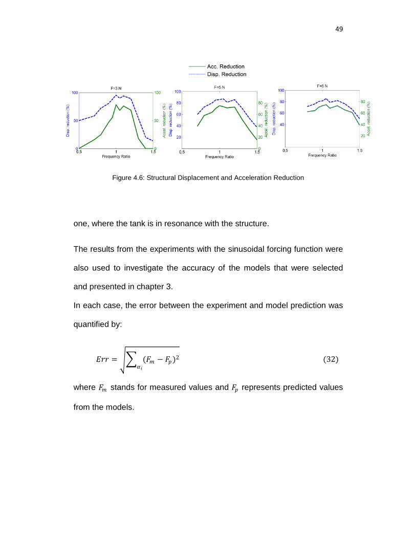
49
Figure 4.6: Structural Displacement and Acceleration Reduction
one, where the tank is in resonance with the structure.
The results from the experiments with the sinusoidal forcing function were
also used to investigate the accuracy of the models that were selected
and presented in chapter 3.
In each case, the error between the experiment and model prediction was
quantified by:
𝐸𝐸𝑓𝑓𝑓𝑓 = �� (𝐹𝐹𝑚𝑚 − 𝐹𝐹𝑝𝑝)2𝛼𝛼𝑠𝑠
(32)
where 𝐹𝐹𝑚𝑚 stands for measured values and 𝐹𝐹𝑝𝑝 represents predicted values
from the models.
50
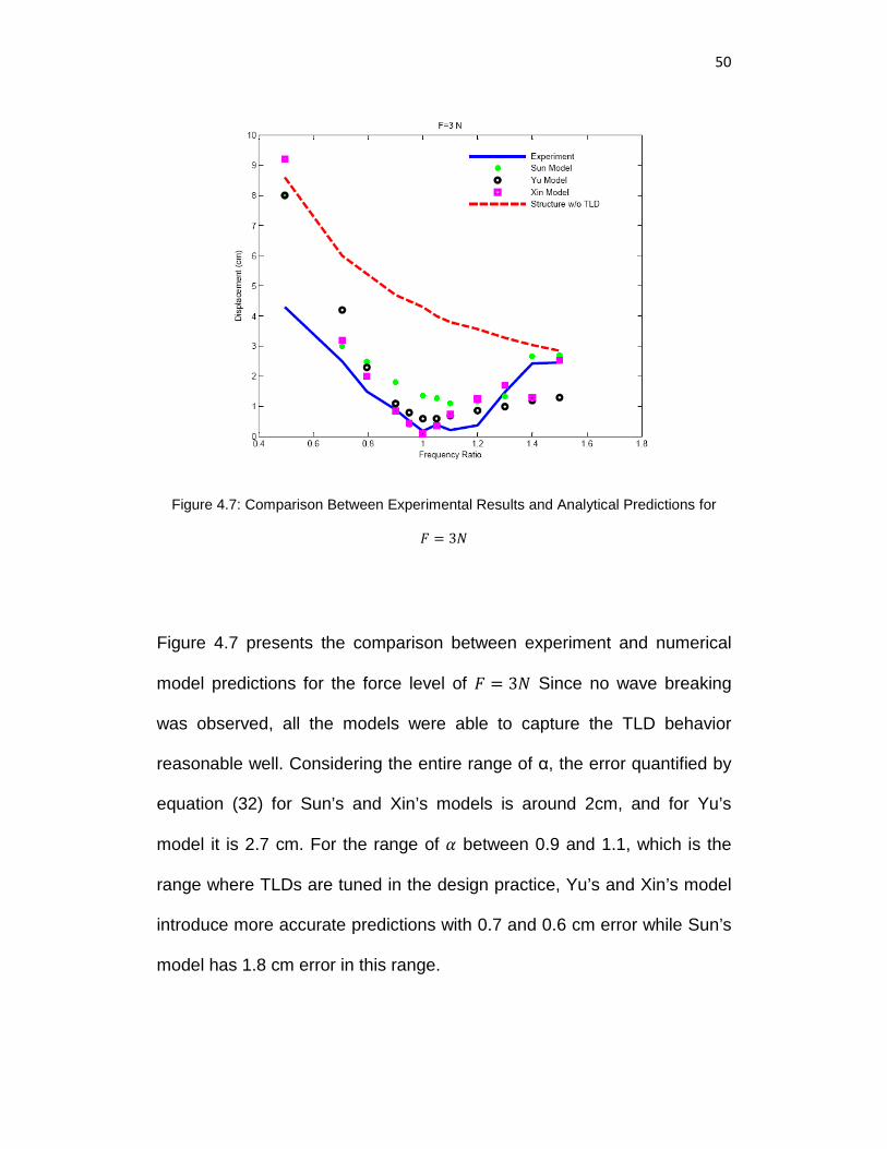
Figure 4.7: Comparison Between Experimental Results and Analytical Predictions for
𝐹𝐹 = 3𝑁𝑁
Figure 4.7 presents the comparison between experiment and numerical
model predictions for the force level of 𝐹𝐹 = 3𝑁𝑁 Since no wave breaking
was observed, all the models were able to capture the TLD behavior
reasonable well. Considering the entire range of α, the error quantified by
equation (32) for Sun’s and Xin’s models is around 2cm, and for Yu’s
model it is 2.7 cm. For the range of 𝛼𝛼 between 0.9 and 1.1, which is the
range where TLDs are tuned in the design practice, Yu’s and Xin’s model
introduce more accurate predictions with 0.7 and 0.6 cm error while Sun’s
model has 1.8 cm error in this range.
51
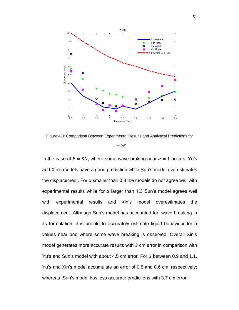
Figure 4.8: Comparison Between Experimental Results and Analytical Predictions for
𝐹𝐹 = 5𝑁𝑁
In the case of 𝐹𝐹 = 5𝑁𝑁, where some wave braking near 𝛼𝛼 = 1 occurs, Yu’s
and Xin’s models have a good prediction while Sun’s model overestimates
the displacement. For α smaller than 0.8 the models do not agree well with
experimental results while for α larger than 1.3 Sun’s model agrees well
with experimental results and Xin’s model overestimates the
displacement. Although Sun’s model has accounted for wave breaking in
its formulation, it is unable to accurately estimate liquid behaviour for α
values near one where some wave breaking is observed. Overall Xin’s
model generates more accurate results with 3 cm error in comparison with
Yu’s and Sun’s model with about 4.5 cm error. For 𝛼𝛼 between 0.9 and 1.1,
Yu’s and Xin’s model accumulate an error of 0.8 and 0.6 cm, respectively;
whereas Sun’s model has less accurate predictions with 3.7 cm error.
52
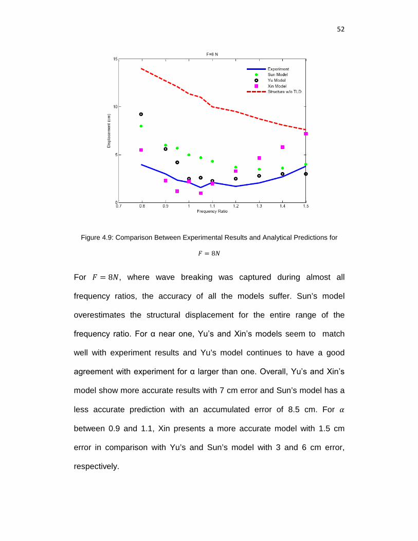
Figure 4.9: Comparison Between Experimental Results and Analytical Predictions for
𝐹𝐹 = 8𝑁𝑁
For 𝐹𝐹 = 8𝑁𝑁, where wave breaking was captured during almost all
frequency ratios, the accuracy of all the models suffer. Sun’s model
overestimates the structural displacement for the entire range of the
frequency ratio. For α near one, Yu’s and Xin’s models seem to match
well with experiment results and Yu’s model continues to have a good
agreement with experiment for α larger than one. Overall, Yu’s and Xin’s
model show more accurate results with 7 cm error and Sun’s model has a
less accurate prediction with an accumulated error of 8.5 cm. For 𝛼𝛼
between 0.9 and 1.1, Xin presents a more accurate model with 1.5 cm
error in comparison with Yu’s and Sun’s model with 3 and 6 cm error,
respectively.
53
Considering all three load cases and the ranges of the frequency ratios,
Yu’s model provides reasonable predictions in both weak and strong wave
breaking and in a broad range of frequency ratios. Xin’s model presents
good results near 𝛼𝛼 = 1 and overestimates the displacement for α larger
than 1.2. Sun’s model can predict the TLD behaviour in the absence of
wave breaking, i.e. 𝐹𝐹 = 3𝑁𝑁, however overestimates the displacements in
the case of wave breaking.
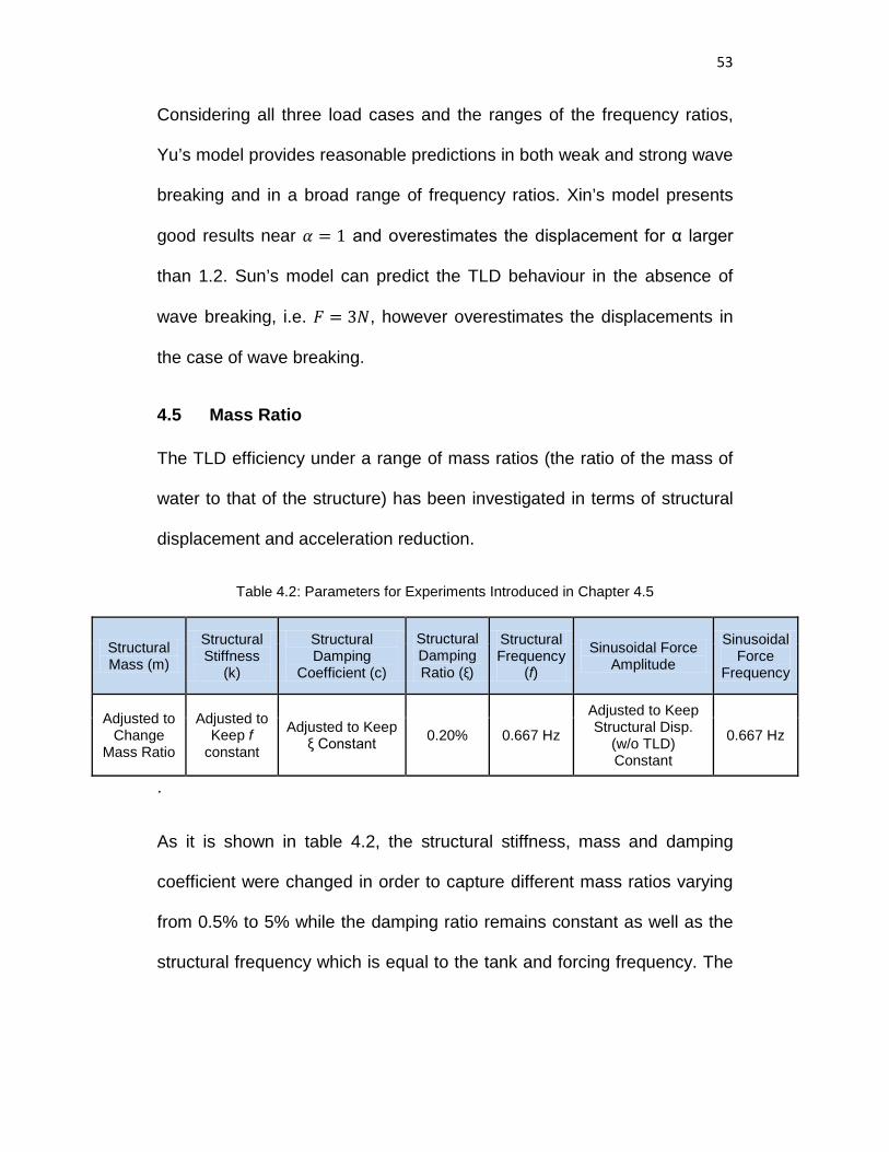
4.5 Mass Ratio
The TLD efficiency under a range of mass ratios (the ratio of the mass of
water to that of the structure) has been investigated in terms of structural
displacement and acceleration reduction.
Table 4.2: Parameters for Experiments Introduced in Chapter 4.5
Structural Mass (m)
Structural Stiffness
(k)
Structural Damping
Coefficient (c)
Structural Damping Ratio (ξ)
Structural Frequency
(f)
Sinusoidal Force Amplitude
Sinusoidal Force
Frequency
Adjusted to Change
Mass Ratio
Adjusted to Keep f
constant
Adjusted to Keep ξ Constant 0.20% 0.667 Hz
Adjusted to Keep Structural Disp.
(w/o TLD) Constant
0.667 Hz
.
As it is shown in table 4.2, the structural stiffness, mass and damping
coefficient were changed in order to capture different mass ratios varying
from 0.5% to 5% while the damping ratio remains constant as well as the
structural frequency which is equal to the tank and forcing frequency. The
54
amplitude of the applied sinusoidal force has been also changed in a way
to reach to the same steady state amplitude in the absence of TLD.
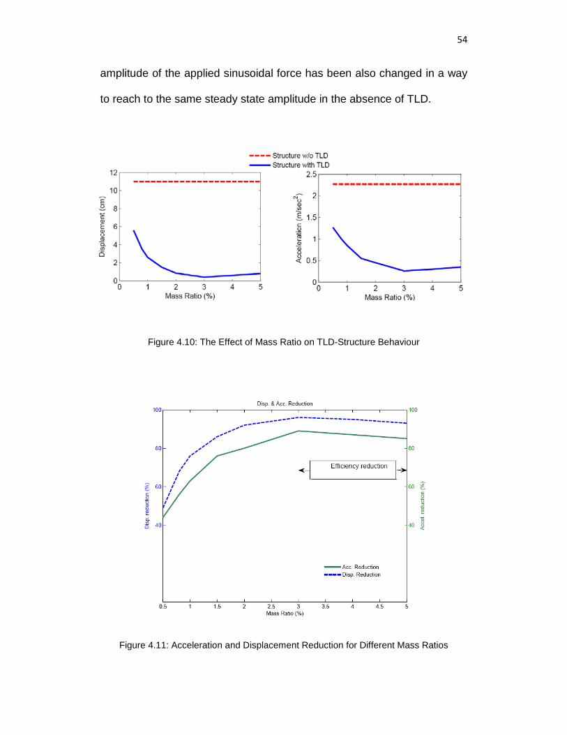
Figure 4.10: The Effect of Mass Ratio on TLD-Structure Behaviour
Figure 4.11: Acceleration and Displacement Reduction for Different Mass Ratios
55
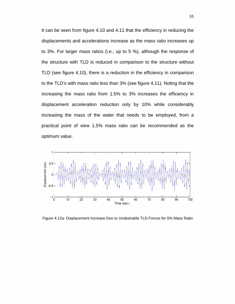
It can be seen from figure 4.10 and 4.11 that the efficiency in reducing the
displacements and accelerations increase as the mass ratio increases up
to 3%. For larger mass ratios (i.e., up to 5 %), although the response of
the structure with TLD is reduced in comparison to the structure without
TLD (see figure 4.10), there is a reduction in the efficiency in comparison
to the TLD’s with mass ratio less than 3% (see figure 4.11). Noting that the
increasing the mass ratio from 1.5% to 3% increases the efficiency in
displacement acceleration reduction only by 10% while considerably
increasing the mass of the water that needs to be employed, from a
practical point of view 1.5% mass ratio can be recommended as the
optimum value.
Figure 4.12a: Displacement Increase Due to Undesirable TLD Forces for 5% Mass Ratio
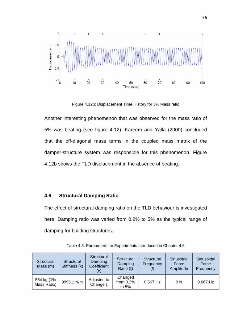
56
Figure 4.12b: Displacement Time History for 3% Mass ratio
Another interesting phenomenon that was observed for the mass ratio of
5% was beating (see figure 4.12). Kareem and Yalla (2000) concluded
that the off-diagonal mass terms in the coupled mass matrix of the
damper-structure system was responsible for this phenomenon. Figure
4.12b shows the TLD displacement in the absence of beating.
4.6 Structural Damping Ratio
The effect of structural damping ratio on the TLD behaviour is investigated
here. Damping ratio was varied from 0.2% to 5% as the typical range of
damping for building structures.
Table 4.3: Parameters for Experiments Introduced in Chapter 4.6
Structural Mass (m)
Structural Stiffness (k)
Structural Damping
Coefficient (c)
Structural Damping Ratio (ξ)
Structural Frequency
(f)
Sinusoidal Force
Amplitude
Sinusoidal Force
Frequency
564 kg (1% Mass Ratio) 9995.1 N/m Adjusted to
Change ξ
Changed from 0.2%
to 5% 0.667 Hz 9 N 0.667 Hz
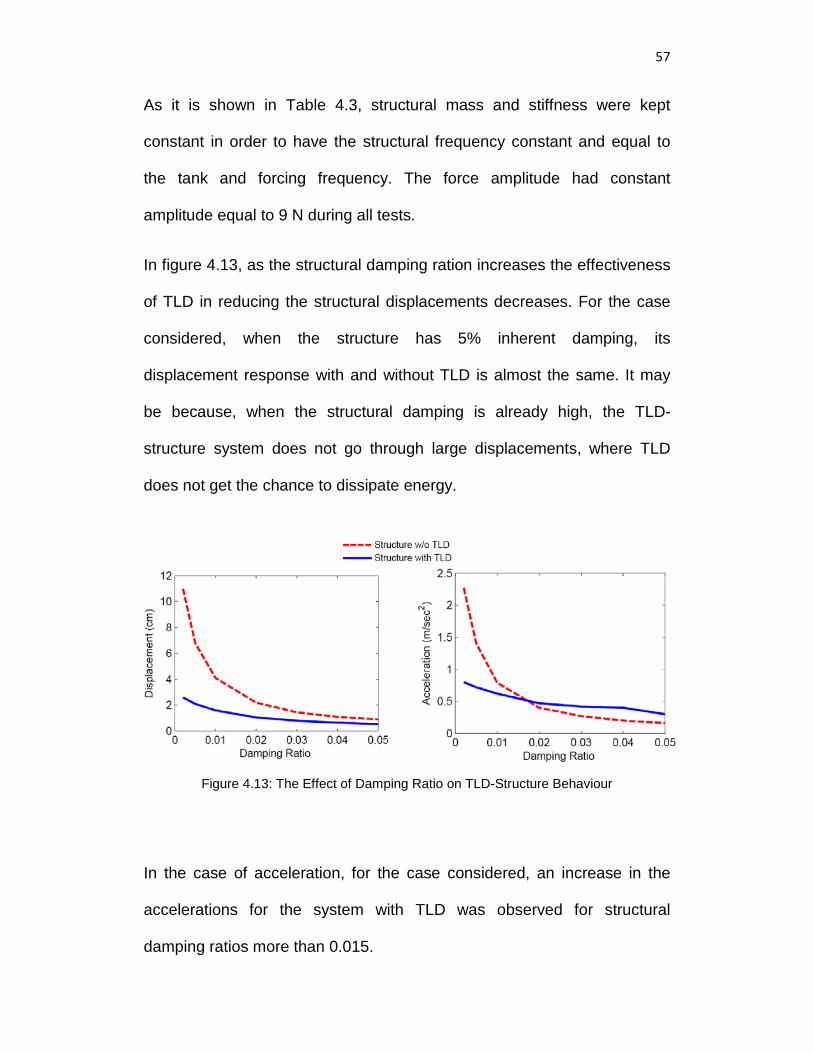
57
As it is shown in Table 4.3, structural mass and stiffness were kept
constant in order to have the structural frequency constant and equal to
the tank and forcing frequency. The force amplitude had constant
amplitude equal to 9 N during all tests.
In figure 4.13, as the structural damping ration increases the effectiveness
of TLD in reducing the structural displacements decreases. For the case
considered, when the structure has 5% inherent damping, its
displacement response with and without TLD is almost the same. It may
be because, when the structural damping is already high, the TLD-
structure system does not go through large displacements, where TLD
does not get the chance to dissipate energy.
Figure 4.13: The Effect of Damping Ratio on TLD-Structure Behaviour
In the case of acceleration, for the case considered, an increase in the
accelerations for the system with TLD was observed for structural
damping ratios more than 0.015.
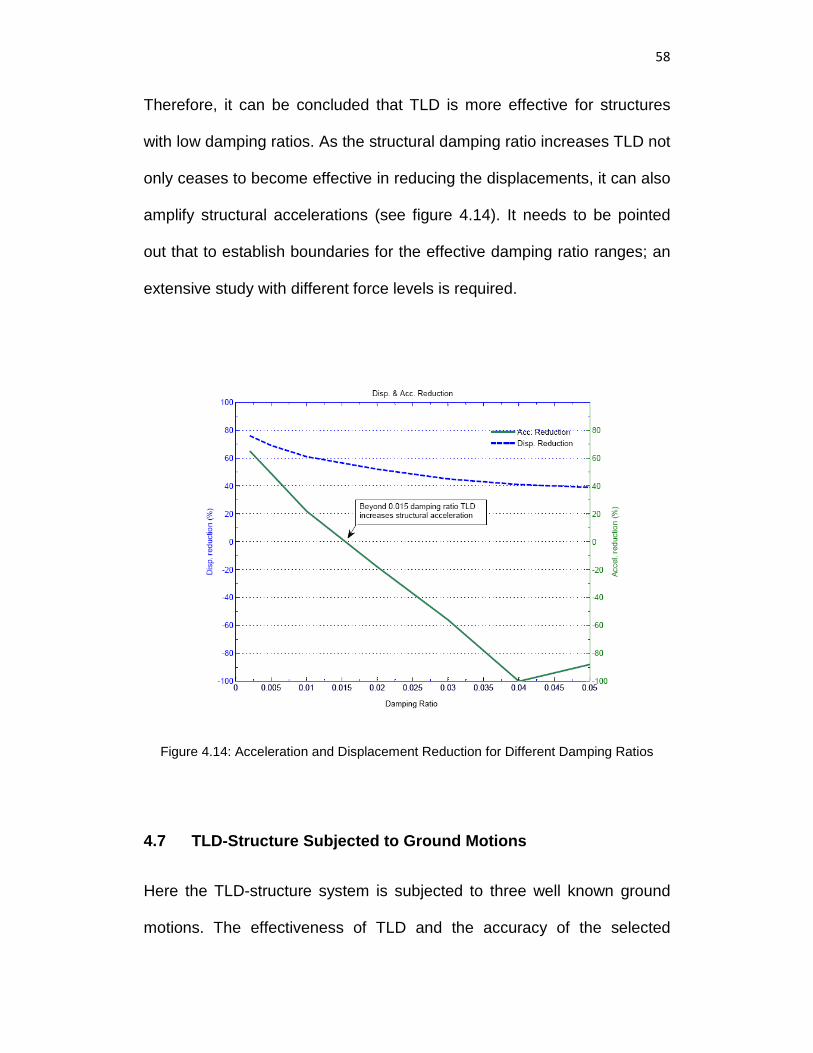
58
Therefore, it can be concluded that TLD is more effective for structures
with low damping ratios. As the structural damping ratio increases TLD not
only ceases to become effective in reducing the displacements, it can also
amplify structural accelerations (see figure 4.14). It needs to be pointed
out that to establish boundaries for the effective damping ratio ranges; an
extensive study with different force levels is required.
Figure 4.14: Acceleration and Displacement Reduction for Different Damping Ratios
4.7 TLD-Structure Subjected to Ground Motions
Here the TLD-structure system is subjected to three well known ground
motions. The effectiveness of TLD and the accuracy of the selected
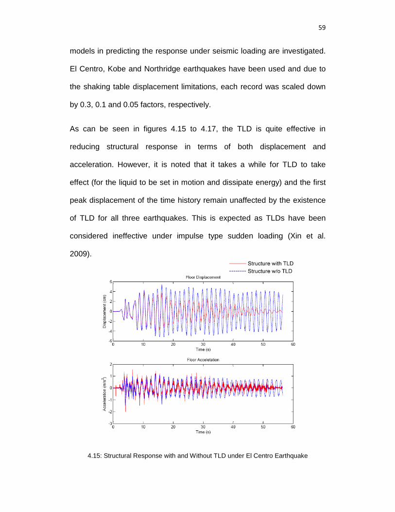
59
models in predicting the response under seismic loading are investigated.
El Centro, Kobe and Northridge earthquakes have been used and due to
the shaking table displacement limitations, each record was scaled down
by 0.3, 0.1 and 0.05 factors, respectively.
As can be seen in figures 4.15 to 4.17, the TLD is quite effective in
reducing structural response in terms of both displacement and
acceleration. However, it is noted that it takes a while for TLD to take
effect (for the liquid to be set in motion and dissipate energy) and the first
peak displacement of the time history remain unaffected by the existence
of TLD for all three earthquakes. This is expected as TLDs have been
considered ineffective under impulse type sudden loading (Xin et al.
2009).
4.15: Structural Response with and Without TLD under El Centro Earthquake
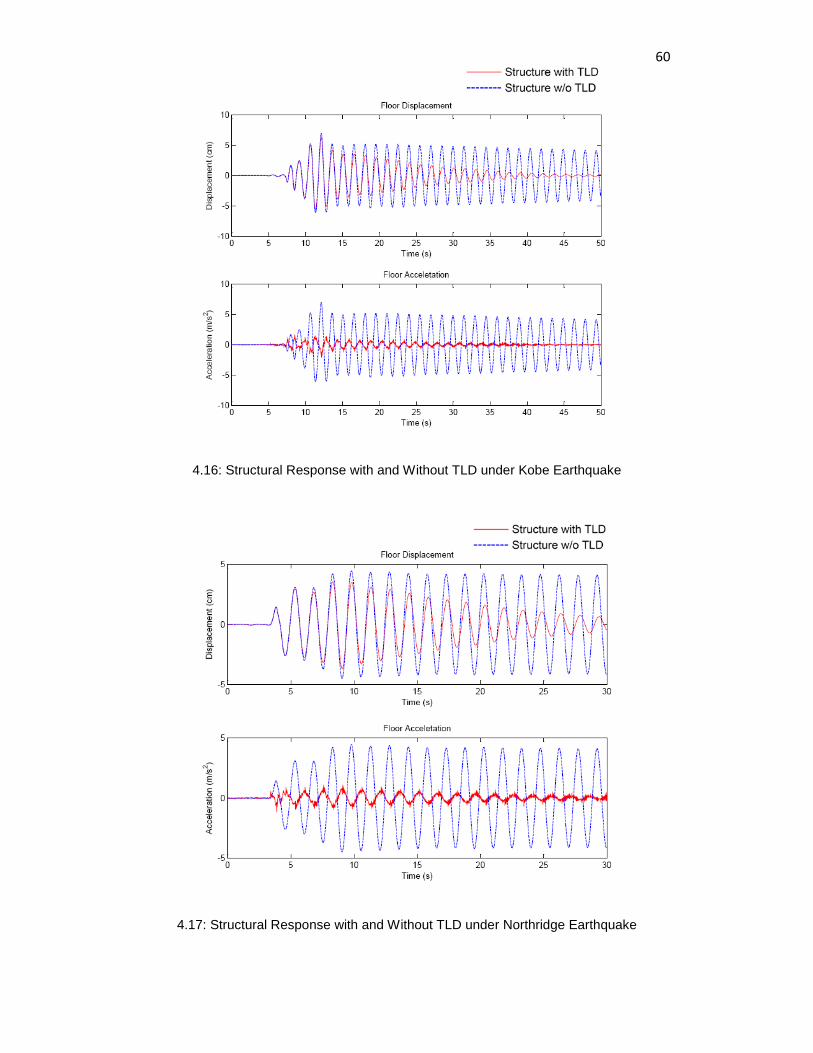
60
4.16: Structural Response with and Without TLD under Kobe Earthquake
4.17: Structural Response with and Without TLD under Northridge Earthquake
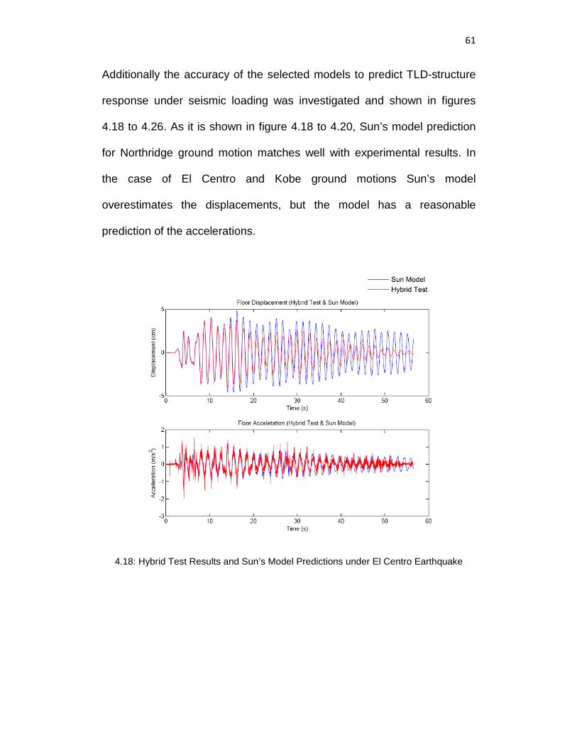
61
Additionally the accuracy of the selected models to predict TLD-structure
response under seismic loading was investigated and shown in figures
4.18 to 4.26. As it is shown in figure 4.18 to 4.20, Sun’s model prediction
for Northridge ground motion matches well with experimental results. In
the case of El Centro and Kobe ground motions Sun’s model
overestimates the displacements, but the model has a reasonable
prediction of the accelerations.
4.18: Hybrid Test Results and Sun’s Model Predictions under El Centro Earthquake
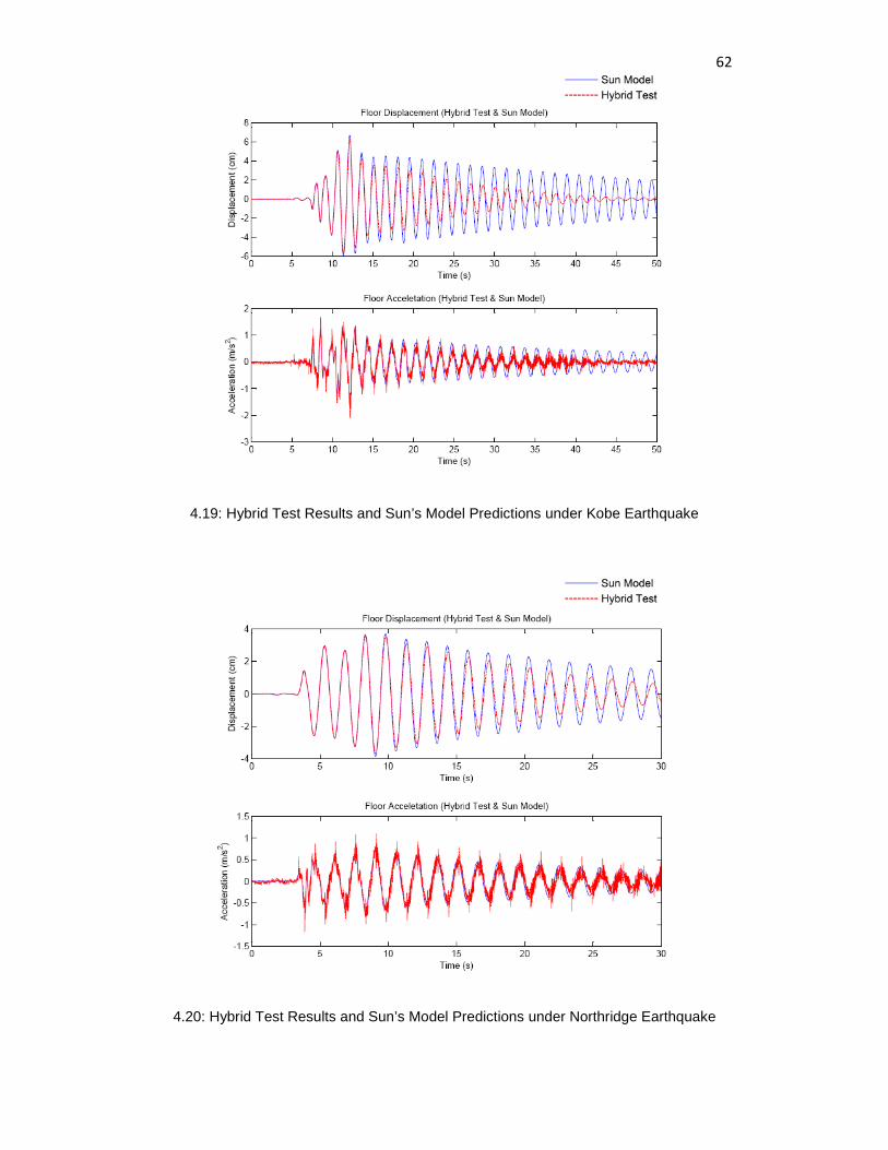
62
4.19: Hybrid Test Results and Sun’s Model Predictions under Kobe Earthquake
4.20: Hybrid Test Results and Sun’s Model Predictions under Northridge Earthquake
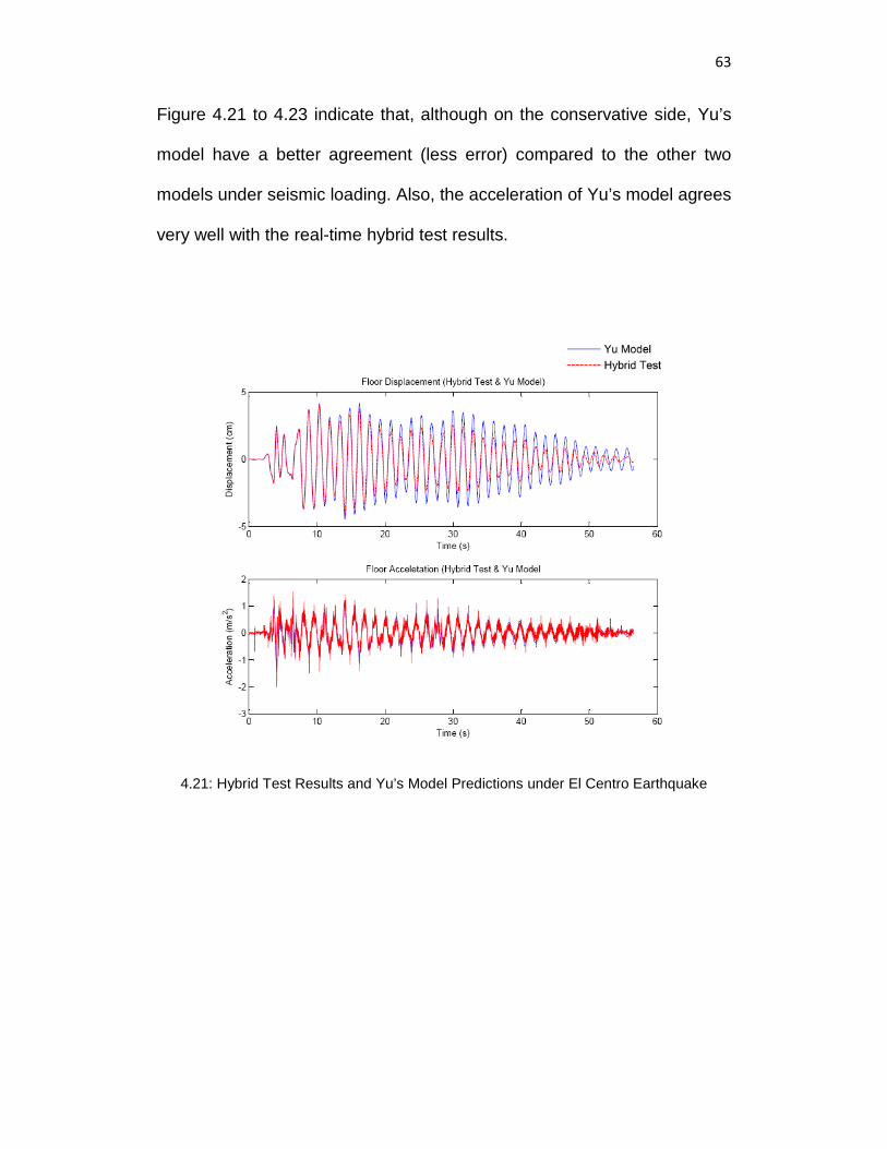
63
Figure 4.21 to 4.23 indicate that, although on the conservative side, Yu’s
model have a better agreement (less error) compared to the other two
models under seismic loading. Also, the acceleration of Yu’s model agrees
very well with the real-time hybrid test results.
4.21: Hybrid Test Results and Yu’s Model Predictions under El Centro Earthquake
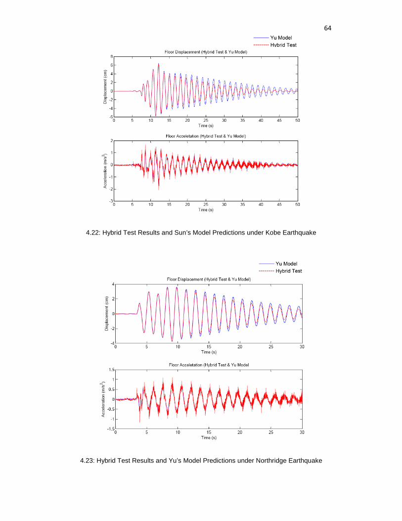
64
4.22: Hybrid Test Results and Sun’s Model Predictions under Kobe Earthquake
4.23: Hybrid Test Results and Yu’s Model Predictions under Northridge Earthquake
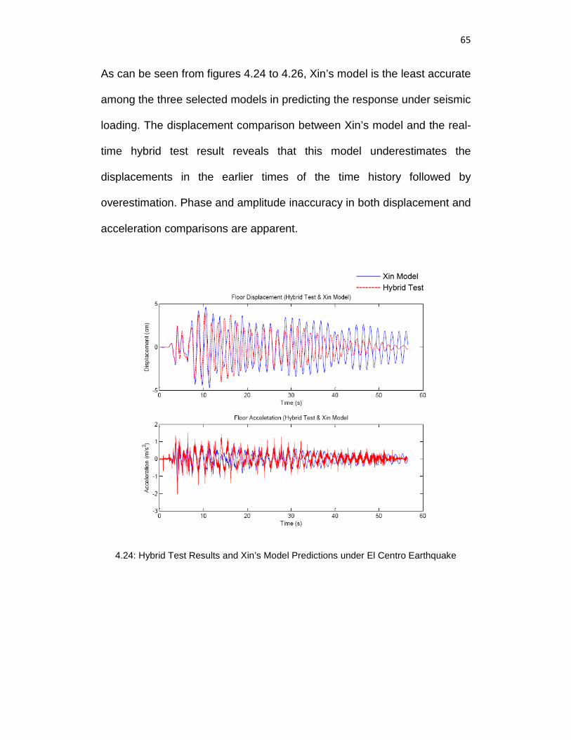
65
As can be seen from figures 4.24 to 4.26, Xin’s model is the least accurate
among the three selected models in predicting the response under seismic
loading. The displacement comparison between Xin’s model and the real-
time hybrid test result reveals that this model underestimates the
displacements in the earlier times of the time history followed by
overestimation. Phase and amplitude inaccuracy in both displacement and
acceleration comparisons are apparent.
4.24: Hybrid Test Results and Xin’s Model Predictions under El Centro Earthquake
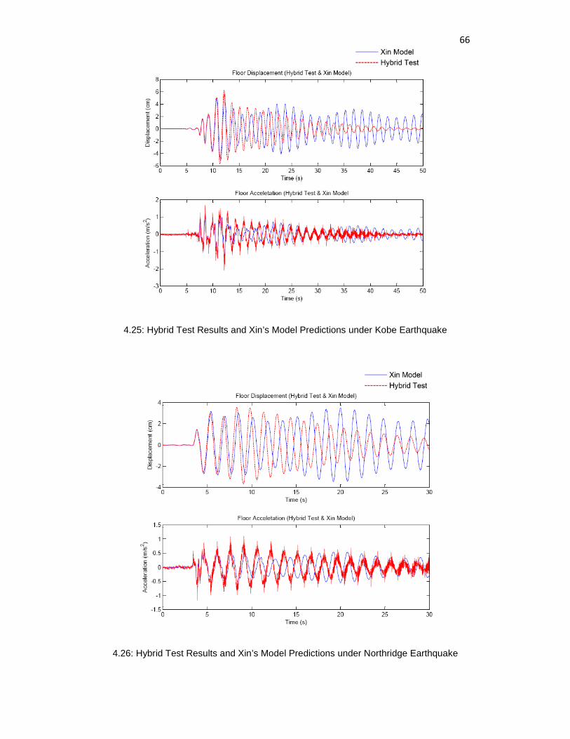
66
4.25: Hybrid Test Results and Xin’s Model Predictions under Kobe Earthquake
4.26: Hybrid Test Results and Xin’s Model Predictions under Northridge Earthquake
67
Investigating the accuracy of the three selected models in comparison to
the real-time hybrid testing results, Yu’s model was found to be more
accurate model in both displacement and acceleration prediction. Sun’s
model has also reasonable enough answers especially in the case of low
amplitude ground accelerations and Xin’s model has the least accuracy
among the three models under seismic loading.
68
Chapter 5
5. Summary and Conclusions
In this study a series of experiments have been conducted with a TLD to
investigate the effects of some of the design parameters of the TLD-
structure system and also to check the accuracy of selected analytical
models in predicting TLD response. These models have been compared
against experimental data when they were first published. Unlike these
studies which provided the comparisons for only a few selected cases, this
study considers a broad range of frequency ration, load amplitude and
types; which also enabled the investigation for determination of effective
frequency ratio, mass ratio, and structural damping ratio. A part of the
experiments were conducted by imposing predefined sinusoidal
displacements to the TLD by using a shake table. The TLD-structure
interaction was investigated by employing real-time hybrid PSD testing
method where the structure was modeled analytically and the TLD was
tested physically in coupled experiment-simulation mode.
Frequency Ratio. Subjecting the TLD to predefined displacement with
various frequencies, it is observed that to design an effective TLD, the
ratio of the structural frequency to that of the TLD should be between 1
and 1.2 when large amount of energy dissipation can be obtained. For
larger frequency ratios frequency ratios, as the inertia and sloshing
69
components of the TLD interface force start canceling each other, the TLD
was observed to be ineffective in dissipating the energy.
Mass Ratio. Looking at the percent displacement and acceleration
reducition for the experiments where the mass ratio (the ratio of the mass
of water to that of the structure) inceases; it has been observed 3% mass
ratio provides the most reduction. Noticing that there is only 10% increase
in TLD efficiency when mass ratio increases from 1.5% to 3%; and
considering practical (space related) issues a mass ratio of 1.5% is
suggested in this study. For mass ratios larger than 3%, beating
phenomenon was observed in the TLD behavior and the efficieny
suffered.
Damping Ratio. It was shown that the TLD is more effective for structures
with low damping ratios where both structural displacements and
accelerations decrease with the introduction of TLD. However, as the
structural damping ratio increases the accelerations start to be amplified
with the introduction of TLD. A dedicated study with several load cases
and different system properties need to be conducted to determine the
boundary of the effective structural damping ratio.
Load Cases. It is observed that for lightly damped structures the TLD is
effective to reduce both structural displacement and acceleration during
harmonic and ground motion displacements. Other common kind of
passive dampers such as hysteretic, viscous, viscoelastic and self-
70
centering systems are usually designed to control structural displacement
and end up amplifying the acceleration response of the structure. It is a
desirable property of TLDs that they are able to reduce both
displacements and accelerations when designed properly.
It is also observed that at the very starting time of the earthquakes the
TLD has not any effect on the structural displacement reduction since the
tank is not set in motion yet.
Accuracy of the Selected Models. The accuracy of three selected
models under different conditions (i.e., different type of loading, levels of
excitation frequency, amplitude of excitation and frequency ratios) were
checked and the following observation were made:
Subjecting TLD-structure system to three sinusoidal loads in the ranges of
both weak and strong wave breaking and calculating accumulative error
between the model predictions and experimental data for each model,
Yu’s model was found introduce reasonable predictions in both weak and
strong wave breaking and in a broad range of frequency ratios. Xin’s
model also presented acceptable results specially near frequency ratio
equal to one and overestimated the displacement for frequency ratios
larger than 1.2. Sun’s model could accurately predict the TLD behaviour in
the absence of wave breaking, and overestimated the displacements
when wave breaking occurred.
71
In the case of three ground motions considered (El Centro, Kobe and
Northridge), Yu was observed to be more accurate in both displacement
and acceleration predictions. Having some overestimations, Sun’s model
had also reasonable enough predictions especially in the case of low
amplitude ground accelerations and Xin’s model predicted structural
response with some inaccuracy in the response amplitude and phase.
From the results of this study, it can be concluded that properly designed
TLD is an effective damper to reduce both structural displacement and
acceleration in the case of ground accelerations and harmonic loads. It is
also economical in comparison with other common kind of dampers.
Investigating the analytical models, it can be concluded that more
accurate models that are able to have a better consideration for wave
breaking occurrence during high amplitude of excitations are required.
Also a more comprehensive experimental/analytical study is necessary to
understand the behavior of TLD under higher mode and structural
nonlinearity effects.
72
Chapter 6
6. References
Abe, M., Fujino, Y., and Kimura, Sh., “Active Tuned Liquid Damper (TLD) with Magnetic Fluid”, Part of the SPIE Corrfrreric€r on Smart Stnuct,mres sad lnteqratecl Systems, Sari Dieqo, California, March (1998), 620 SPIE Vol 3329 • 0277-78f5X/98/S1O Oh
Banerji, P., Murudi, M., Shah, A. H., and Popplewell, N., “Tuned liquid
dampers for controlling earthquake response of structures”, Earthquake Engineering and Structural Dynamics (2000), Vol. 29, pp. 587-602.
Bauer, H. F., “Oscillations of Immiscible Liquids in a Rectangular
Container”, Journal of Sound and Vibration (1984), Vol. 93(l), pp. 117-133.
Biswal, K.C., Bhattacharyya, S.K., and Sinha, P.K, “Free-Vibration
Analysis of Liquid-Filled Tank with Baffles, Journal of Sound and Vibration” (2003), Vol. 259(1), pp. 177-192.
Biswal, K.C., Bhattacharyya, S.K., and Sinha, P.K., “Dynamic response
analysis of a liquid-filled cylindrical tank with annular baffle”, Journal of Sound and Vibration (2004), Vol. 274, pp. 13–37.
Casciati, Fabio, De Stefano, Alessandro, Matta, Emiliano, “Simulating a
conical tuned liquid damper”, Simulation Modelling Practice and Theory (2003), Vol. 11, pp. 353–370.
Cassolato, M. R., Love, J. S., and Tait, M. J., “Modelling of a Tuned Liquid
Damper with Inclined Damping Screens”, Structural Control and Health Monitoring (2010), John Wiley & Sons, Ltd.
Chang, C.C., and Gu, M., “Suppression of Vortex-Excited Vibration of Tall
Buildings using Tuned Liquid Damper”, Journal of Wind Engineering and Industrial Aerodynamic 83 (1999), pp. 225-237.
Chen, Y., and Ko, C., “Active Tuned Liquid Column Damper with
Propellers”, Earthquake Engineering and Structural Dynamics (2003), Vol. 32, pp. 1627–1638
73
Christopoulos, C., and Filiatrault, A., “Principles of Passive Supplemental
Damping and Seismic Isolation”, IUSS Press, Pavia – Italy (2006). Deng, X., and Tait, M.J., “Theoretical Modeling of TLD with Different Tank
Geometries Using Linear Long Wave Theory”, Journal of Vibration and Acoustics (2009), Vol. 131 / 041014-1.
Fediw, A.A., Isyumov, N., Vickery, B.J., “Performance of a tuned sloshing
water damper”, Journal of Wind Engineering and Industrial Aerodynamics (1995), Vol. 57, pp. 237–247.
Frandsen, J.B., “Numerical Predictions of Tuned Liquid Tank Structural
Systems”, Journal of Fluids and Structures (2005), Vol. 20, pp. 309–329.
Gardarsson, S. M., “Shallow-water Sloshing”, PhD. Thesis, University of
Washington, Seattle, 1997. Gardarsson, S., Yeh, H., and Reed, D., “Behaviour of Sloped-Bottom
Tuned Liquid Dampers”, Journal of Engineering Mechanics (2001), Vol. 127, No. 3.
Idir, Meziane, Ding, Xiaohua, and Chen, Genda, “Fundamental Frequency
of Water Sloshing Waves in a Sloped-Bottom Tank as Tuned Liquid Damper”, ASCE (2009).
Ikeda, Takashi, “Nonlinear Parametric Vibrations of an Elastic Structure
with a Rectangular Liquid Tank”, Nonlinear Dynamics (2003), Vol. 33, pp. 43–70.
Ikeda, Takashi, and Ibrahim, R.A., “Nonlinear random responses of a
structure parametrically coupled with liquid sloshing in a cylindrical tank”, Journal of Sound and Vibration (2005), Vol. 284, pp. 75–102.
Ikeda, T., “Non-Linear Dynamic Responses of Elastic Two-Story
Structures with Partially Filled Liquid Tanks, International Journal of Non-Linear Mechanics 45 (2010), pp. 263–278.
Kaneko, S., Ishikawa, M., “Modeling of Tuned Liquid Damper With
Submerged Nets”, Applied Mechanics International Mechanical Engineering Congress & Exposition (1999).
Kareem, A., and Sun, W.-J., “Stochastic Response of Structures with
Fluid-Containing Appendages”, Journal of Sound and Vibration (1987), Vol. 119, No. 3.
74
Kareem, A., Yalla, S., and McCullough, M., “Sloshing-Slamming Dynamics
– S2 – Analogy for uned Liquid Dampers”, Vibro-Impact Dynamics of Ocean Systems (2009), LNACM 44, pp. 123–133.
Kim, Y., You, K., Cho, J., and Hong, D., “The Vibration Performance
Experiment of Tuned Liquid Damper and Tuned Liquid Column Damper”. Journal of Mechanical Science and Technology (2006), Vol. 20, No.6, pp. 795-805.
Koh, C. G., Mahatma, S., and Wang, C. M., “Reduction of structural
vibrations by multiple-mode liquid dampers”, Engineering Structures (1995), Vol. 17, No. 2.
Lee, S. C., and Reddy, D. V., “Frequency Tuning of Offshore Platform by
Liquid Sloshing”, Applied Ocean Research (1982), Vol. 4, pp. 226–231. Lee, Sung-Kyung, Park, Eun Churn, Min, Kyung-Won, Lee, Sang-Hyun,
Chung, Lan, and Park, Ji-Hun, “Real-time Hybrid Shaking Table Testing Method for the Performance Evaluation of a Tuned Liquid Damper Controlling Seismic Response of Building Structures”, Journal of Sound and Vibration (2007), Vol. 302, pp. 596–612.
Lepelletier, TG, Raichlen, F., “Nonlinear oscillations in rectangular tanks”,
J Eng Mech (1988), Vol. 114, pp. 1–23. Lieping, Y., Xinzheng, L., Zhe, Q., and Jianqun, H., “Distributed TLDs in
RC floors and their vibration reduction efficiency”, Earthquake Engineering and Engineering Vibration (2008), Vol. 7, pp. 107-112.
Li, H., and Wang Y., “Theoretical and Experimental Studies on Reduction
foe Multi-Modal Seismic Response of High-Rise Structure by Tuned Liquid Dampers”, Journal of Vibration and Control (2004), Vol. 10, 1041.
Li, S.J., Li, G.Q., Tang, J., and Li, Q.S., “Shallow Rectangular TLD for
Structural Control Implementation”, Applied Acoustics 63 (2002), pp. 1125–1135.
Mei, C. C., “Numerical Methods in Water-Wave Diffraction and Radiation”,
Ann. Rev. Fluid Mech. (1978), Vol. 10, pp. 393-416. Modi, V. J., and Welt, F., “Damping of Wind Induced Oscillations Through
Liquid Sloshing”, Preprint Vol. 5, Seventh International Conference on Wind Engineering (1987), Aachen, W. Germany, July 6-10.
75
Modi, V.J., and Seto, M.L., “Suppression of Flow-Induced Oscillations using Sloshing Liquid Dampers: Analysis and Experiments”, Journal of Wind Engineering and Industrial Aerodynamics 67& 68 (1997), pp. 611-625.
Modi, V.J., and Akinturk, A., “An Efficient Liquid Sloshing Damper for
Control of Wind-Induced Instabilities”, Journal of Wind Engineering and Industrial Aerodynamics 90 (2002), pp. 1907–1918
Ohyama. T., and Fujii, K., “A Boundary Element Analysis for Two-
dimentional Nonlinear Sloshing Problem”, Journal of Structural Engineering (1989), Vol. 35A, pp. 575-584, (In Japanese).
Olson, D. E., Reed, D. A., “A nonlinear numerical model for sloped-bottom
tuned liquid dampers”, Earthquake Engineering and Structural Dynamics (2001), Vol. 30, pp. 731-743.
Ramaswamy, B., Kawahara, M., Nakayama, T., “Lagrangian finite element
method for the analysis of two-dimensional sloshing problems”, Int J Numer Methods Fluids (1986), Vol. 6, pp. 659–70.
Reed D., Yu J., Yeh, H., and Gardarsson S., “Investigation of tuned liquid
dampers under Large amplitude excitation”, Journal of Engineering Mechanics (1998), Vol. 124, No. 4, pp. 405-413.
Sakai F., Takaeda S., and Tamaki T., “Tuned Liquid Column Damper –
New type device for suppression of building vibrations”, Proc. of International Conference on High-rise Buildings (1989), Vol. 2, Nanjing, China.
Samanta, A., and Banerji, P., “Structural Vibration Control using Modified
Tuned Liquid Dampers”, The IES Journal Part A: Civil & Structural Engineering (2010), Vol. 3, No. 1, pp. 14–27.
Sato, T., Japan Journal of Wind Engineering (1987), Vol. 32, pp. 67-68. Seto ML., “An investigation on the suppression of fluid induced vibrations
of bluff bodies”, Ph.D. Thesis, The University of British Columbia, Canada, 1996.
Shimisu T., and Hayama, S., “Nonlinear Response of Sloshing Based on
the Shallow water Wave Theory”, The Japan Society of Mechanical Engineers (1986), No. 86-0385A.
Siddique, M.R., and Hamed M.S., “A Nonlinear Numerical Model for
Sloshing Motion in Tuned Liquid Dampers, International Journal for
76
Numerical Methods in Heat & Fluid Flow (2005), Vol. 15 No. 3, pp. 306-324.
Sun, Li Min, Fujino, Yozo, Pacheco, Benito M., and Isobe, Masahiko,
“Nonlinear Waves and Dynamic Pressure in Rectangular Tuned Liquid Damper (TLD)”, Structural Engineering/Earthquake Engineering (1989), Vol.6. No. 2, pp. 251s-262s.
Sun, Li Min, “Semi-Analytical modeling of Tuned Liquid Damper (TLD)
with Emphesis on Damping of Liquid Sloshing”, PhD Thesis, University of Tokyo, Japan, 1991.
Sun, L. M., Fujino, Y., Pacheco, M., and Chaiseri, P., “Modelling of Tuned
Liquid Damper (TLD)”, Journal of Wind Engineering and Industrial Aerodynamics (1992), pp. 41-44.
Sun, L. M., Fujino, Y., Chaiseri, P., and Pacheco, M., “The Properties of
Tuned Liquid Dampers Using a TMD Analogy”, Earthquake Engineering and Structural Dynamics (1995), VOL. 24, pp. 967-976.
Tait, M. J., El Damatty, A. A., and Isyumov, N., “An Investigation of Tuned
Liquid Dampers Equipped with Damping Screens under 2D Excitation”, Earthquake Engineering and Structural Dynamics (2005), Vol. 34, pp. 719–735.
Tait, M.J., El Damatty, A.A., Isyumov, N., and Siddique, M.R., “Numerical
Flow Models to Simulate Tuned Liquid Dampers (TLD) with Slat Screens”, Journal of Fluids and Structures (2005), Vol. 20, pp. 1007–1023.
Tait, M. J., Isyumov, N., and El Damatty, A. A., “Effectiveness of a 2D TLD
and Its Numerical Modeling”, Journal of Structural Engineering (2007), Vol. 133, No. 2, pp. 251–263.
Tait, M.J., “Modelling and preliminary design of a structure-TLD system”,
Engineering Structures (2008), Vol. 30, 2644–2655. Tamura, Y., Fujii, K., Ohtsuki, T., Wakahara, T., and Kohsaka, R.,
“Effectiveness of tuned liquid dampers under wind excitation”, Engineering Structures (1995), Vol. 17, No. 9, pp. 609-621.
Toshiyuki, N., and Tanaka, Y., ‘‘Study on a vibration damper system using
hydra-dynamic force of sloshing’’, In summarize of Technical Papers of Annual Meeting Architectural Institute of Japan, pp. 563–570.
77
Ueda T., Nakagaki R., and Koshida K., “Supression of wind induced vibration by dynamic dampers in tower-like structures”, Journal of Wind Engineering and Industrial Aerodynamics (1992), 41-44, pp. 1907-1918.
Vandiver, J. K., and Mitome, S., ‘‘Effect of liquid storage tanks on the
dynamic response of offshore platform,’’ Applied Ocean Research 1 (1979), pp. 67–74.
Wakahara, T., Ohyama, T., and Fujii, K., “Suppression of Wind-Induced
Vibration of a Tall Building using Tuned Liquid Damper”, Journal of Wind Engineering and Industrial Aerodynamics (1992), 41-4.4, pp. 1895-1906.
Wang, Z., “High-rise Structure Vibration Control”, Tongji University (1996),
(in Chinese) Warnitchai, P., and Pinkaew, T., “Modelling rectangular Dampening of
liquid sloshing in tanks with flowdevices”, Engineering Structures (1998), Vol. 20, No 7, pp. 593-600.
Xin, Yuxiang , “Seismic Performance of Mass-Variable Tuned Liquid
Dampers With Particles Fluidization In Building Application”, PhD Thesis, University of Missouri-Rolla, United States, 2006.
Xin, Yuxiang, Chen, Genda, and Menglin, Lou, “Seismic response control
with density-variable tuned liquid dampers”, Earthquake Engineering and Engineering Vibration (2009), Vol. 8, pp. 537-546.
Yalla, S. K., Kareem, A., “Beat phenomenon in combined structure-liquid
damper systems”, Engineering Structures 23 (2001), pp. 622–630. Yamamoto, T., Yoshida A., and Ijima, T., “Dynamics of Elastically Moored
Floating Objects”, In: C.L. Kirk, Editor, Dynamics Analysis of Offshore Structures, CML, Southampton (1982).
Yamamoto, K., and Kawahara, M., “Structural oscillation control using
tuned liquid damper”, Comput Struct (1999), Vol. 71, pp. 435–46. You, K., Kim, Y. M., Yang, C. M., and Hong, D. P., “Increasing Damping
Ratios in a Tuned Liquid Damper using Damping Bars”, Key Engineering Materials Vols. 353-358 (2007), pp 2652-2655.
Yu, Jin-Kyu, “Nonlinear Characteristics of Tuned Liquid Dampers”, PhD
Thesis, University of Washington, United States, 1997.
78
Yu, Jin-Kyu, Wakahara, Toshihiro, and Reed, Dorothy A., “A Non-linear Numerical Model of the Tuned Liquid Damper”, Earthquake Engineering and Structural Dynamics (1999), Vol. 28, pp. 671-686.
Zang, Y., Xue, S., Kurita, S., “A boundary element method and spectral
analysis model for small-amplitude viscous fluid sloshing in couple with structural vibrations”, Int J Numer Methods Fluids (2000); Vol. 32, pp. 79–96.
79
Appendix A
A. Solution of the Basic Equations for Sun’s Model
A.1 Non-dimensionalization of Basic Equations
In order to solve equations (5) and (6) they are non-dimensionalized using
the following dimensionless variables:
��𝑥 = 𝑥𝑥𝑎𝑎
; ��𝑧 = 𝑧𝑧ℎ
; ��𝜂 = 𝜂𝜂ℎ
; 𝜀𝜀 = ℎ𝑎𝑎
; ��𝜕 = 𝜕𝜕𝐶𝐶0
; ��𝜕 = 𝜕𝜕𝜕𝜕0
; ��𝑘 = 𝑘𝑘𝑎𝑎; ��𝑥��𝑠 = 𝜕𝜕02
𝑎𝑎��𝑥𝑠𝑠; ��𝜔 = 𝜔𝜔𝜕𝜕0
where 𝐶𝐶0 = �𝑔𝑔ℎ is the wave velocity and 𝜕𝜕0 = 𝑎𝑎 𝐶𝐶0⁄ .
Multiplying equation (5) by 𝜕𝜕0 ℎ⁄ and equation (6) by 𝜕𝜕0 𝐶𝐶0⁄ the non-
dimenionalized basic equations (without considering wave breaking
effects) are obtained as
𝜕𝜕��𝜂𝜕𝜕��𝜕
+ σ𝜕𝜕(𝜙𝜙��𝜕)𝜕𝜕��𝑥
= 0 (𝑤𝑤 − 1)
𝜕𝜕��𝜕𝜕𝜕��𝜕
+ �1 − 𝑇𝑇𝑔𝑔2���𝜕𝜕𝜕��𝜕𝜕𝜕��𝑥
+𝜕𝜕��𝜂𝜕𝜕��𝑥
+ 𝜎𝜎𝜙𝜙𝜀𝜀2 𝜕𝜕2��𝜂𝜕𝜕��𝑥2
𝜕𝜕��𝜂𝜕𝜕��𝑥
= −��𝜆��𝜕 − ��𝑥𝑠𝑠 (𝑤𝑤 − 2)
where ��𝜕 = 0 at the end walls and the dimensionless damping coefficient is
��𝜆 =1
(��𝜂 + 1)8
3𝜋𝜋𝜀𝜀𝐶𝐶0�𝜕𝜕𝑙𝑙𝑣𝑣 �1 + �
2ℎ𝑏𝑏� + 𝑆𝑆� (𝑤𝑤 − 3)
A.2 Discretization of Basic Equations
Equations (A-1) and (A-2) are discretized with respect to 𝑥𝑥 into 𝑛𝑛 divisions.
Then, using finite difference approximation and based on backward Tailor
series new equations are obtained. Finally, by employing Runge-Kutta-Gill
80
method the equations are solved in the time domain in order to find
dimensionless values of 𝜕𝜕 and 𝜂𝜂.
The value of 𝑛𝑛 is suggested as [64]
𝑛𝑛 =𝜋𝜋
[2𝑎𝑎𝑓𝑓𝑐𝑐𝑐𝑐𝑎𝑎𝑠𝑠�𝜕𝜕𝑎𝑎𝑛𝑛ℎ (𝜋𝜋𝜀𝜀) 2tanh(𝜋𝜋𝜀𝜀 2)⁄⁄ ] (𝑤𝑤 − 4)
Considering first mode of liquid sloshing, dimensionless wave number is
found as ��𝑘 = 𝜋𝜋 2⁄ .
Equations (A-1) and (A-2) can be written in the following form:
𝜕𝜕��𝜂𝜕𝜕��𝜕
+ σ𝜕𝜕(𝜙𝜙��𝜕)𝜕𝜕��𝑥
= 0 (𝑤𝑤 − 5)
𝜕𝜕��𝜕𝜕𝜕��𝜕
+ 𝑔𝑔𝜕𝜕𝐾𝐾𝜕𝜕��𝑥
+𝜕𝜕��𝜂𝜕𝜕��𝑥
+ 𝐶𝐶𝜕𝜕𝑀𝑀𝜕𝜕��𝑥
= −��𝜆��𝜕 − ��𝑥𝑠𝑠 (𝑤𝑤 − 6)
where 𝑔𝑔 = (1/2)�1 − 𝑇𝑇𝑔𝑔2�; 𝐾𝐾 = ��𝜕2; 𝐶𝐶 = 𝜎𝜎𝜙𝜙𝜀𝜀2; and 𝑀𝑀 = (1 2)(𝜕𝜕��𝜂 𝜕𝜕��𝑥⁄ )2⁄
Then, equations (A-5) and (A-6) are discritized in x using backward Tailor
series and obtained as
𝜕𝜕��𝜂𝜕𝜕��𝜕
= −σ(𝜙𝜙𝑠𝑠+1��𝜕𝑠𝑠+1 − 𝜙𝜙𝑠𝑠��𝜕𝑠𝑠)
𝛥𝛥��𝑥= σ
(𝜙𝜙𝑠𝑠��𝜕𝑠𝑠 − 𝜙𝜙𝑠𝑠+1��𝜕𝑠𝑠+1)𝛥𝛥��𝑥
,
𝑠𝑠 = 1~𝑛𝑛 − 1 (𝑤𝑤 − 7)
𝜕𝜕��𝜂𝜕𝜕��𝜕
= −σ(𝜙𝜙1��𝜕1 − 𝜙𝜙0��𝜕0)
𝛥𝛥𝑥𝑥/2= −2σ
(𝜙𝜙1��𝜕1)𝛥𝛥��𝑥
, 𝑠𝑠 = 0 (𝑤𝑤 − 8)
𝜕𝜕��𝜂𝜕𝜕��𝜕
= −σ(𝜙𝜙𝑛𝑛+1��𝜕𝑛𝑛+1 − 𝜙𝜙𝑛𝑛��𝜕𝑛𝑛)
𝛥𝛥��𝑥/2= 2σ
(𝜙𝜙𝑛𝑛��𝜕𝑛𝑛)𝛥𝛥��𝑥
, 𝑠𝑠 = 𝑛𝑛 (𝑤𝑤 − 9)
𝜕𝜕��𝜕𝜕𝜕��𝜕
= �1𝛥𝛥��𝑥� (��𝜂𝑠𝑠−1 − ��𝜂𝑠𝑠 + 𝑔𝑔𝑠𝑠(𝐾𝐾𝑠𝑠−1 − 𝐾𝐾𝑠𝑠) + 𝐶𝐶𝑠𝑠(𝑀𝑀𝑠𝑠−1 − 𝑀𝑀𝑠𝑠) − ��𝜆��𝜕 − ��𝑥𝑠𝑠 , 𝑠𝑠
= 1~𝑛𝑛 (𝑤𝑤 − 10)
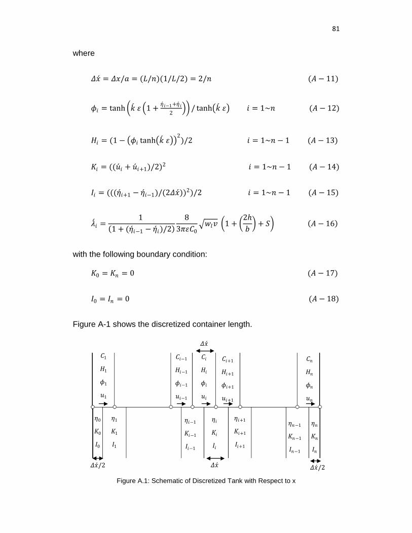
81
where
𝛥𝛥��𝑥 = 𝛥𝛥𝑥𝑥/𝑎𝑎 = (𝐿𝐿/𝑛𝑛)(1/𝐿𝐿/2) = 2/𝑛𝑛 (𝑤𝑤 − 11)
𝜙𝜙𝑠𝑠 = tanh ���𝑘 𝜀𝜀 �1 + ��𝜂 𝑠𝑠−1+��𝜂 𝑠𝑠2
�� / tanh���𝑘 𝜀𝜀� 𝑠𝑠 = 1~𝑛𝑛 (𝑤𝑤 − 12)
𝑔𝑔𝑠𝑠 = (1 − �𝜙𝜙𝑠𝑠 tanh���𝑘 𝜀𝜀��2
)/2 𝑠𝑠 = 1~𝑛𝑛 − 1 (𝑤𝑤 − 13)
𝐾𝐾𝑠𝑠 = ((��𝜕𝑠𝑠 + ��𝜕𝑠𝑠+1)/2)2 𝑠𝑠 = 1~𝑛𝑛 − 1 (𝑤𝑤 − 14)
𝑀𝑀𝑠𝑠 = (((��𝜂𝑠𝑠+1 − ��𝜂𝑠𝑠−1)/(2𝛥𝛥��𝑥))2)/2 𝑠𝑠 = 1~𝑛𝑛 − 1 (𝑤𝑤 − 15)
��𝜆𝑠𝑠 =1
(1 + (��𝜂𝑠𝑠−1 − ��𝜂𝑠𝑠)/2)8
3𝜋𝜋𝜀𝜀𝐶𝐶0�𝜕𝜕𝑙𝑙𝑣𝑣 �1 + �
2ℎ𝑏𝑏� + 𝑆𝑆� (𝑤𝑤 − 16)
with the following boundary condition:
𝐾𝐾0 = 𝐾𝐾𝑛𝑛 = 0 (𝑤𝑤 − 17)
𝑀𝑀0 = 𝑀𝑀𝑛𝑛 = 0 (𝑤𝑤 − 18)
Figure A-1 shows the discretized container length.
Figure A.1: Schematic of Discretized Tank with Respect to x
𝐶𝐶1
𝑔𝑔1
𝜙𝜙1
𝜕𝜕1
𝜂𝜂𝑛𝑛
𝐾𝐾𝑛𝑛
𝑀𝑀𝑛𝑛
𝐶𝐶𝑛𝑛
𝑔𝑔𝑛𝑛
𝜙𝜙𝑛𝑛
𝜕𝜕𝑛𝑛
𝐶𝐶𝑠𝑠−1
𝑔𝑔𝑠𝑠−1
𝜙𝜙𝑠𝑠−1
𝜕𝜕𝑠𝑠−1
𝐶𝐶𝑠𝑠+1
𝑔𝑔𝑠𝑠+1
𝜙𝜙𝑠𝑠+1
𝜕𝜕𝑠𝑠+1
𝐶𝐶𝑠𝑠
𝑔𝑔𝑠𝑠
𝜙𝜙𝑠𝑠
𝜕𝜕𝑠𝑠
𝜂𝜂0
𝐾𝐾0
𝑀𝑀0
𝜂𝜂𝑠𝑠
𝐾𝐾𝑠𝑠
𝑀𝑀𝑠𝑠
𝜂𝜂𝑠𝑠+1
𝐾𝐾𝑠𝑠+1
𝑀𝑀𝑠𝑠+1
𝜂𝜂𝑠𝑠−1
𝐾𝐾𝑠𝑠−1
𝑀𝑀𝑠𝑠−1
𝜂𝜂𝑛𝑛−1
𝐾𝐾𝑛𝑛−1
𝑀𝑀𝑛𝑛−1
𝜂𝜂1
𝐾𝐾1
𝑀𝑀1
𝛥𝛥��𝑥/2 𝛥𝛥��𝑥/2 𝛥𝛥��𝑥
𝛥𝛥��𝑥
82
Then, the descritized equations are solved with Runge-Kutta-Gill method
in time.
A.3 Runge-Kutaa-Gill Method
The equations (A-7) to (A-10) can be defined in the vector form as
𝜕𝜕𝜂𝜂𝜕𝜕��𝜕
= 𝑓𝑓(𝜕𝜕, 𝜂𝜂,𝜕𝜕) (𝑤𝑤 − 19)
𝜕𝜕𝜕𝜕𝜕𝜕��𝜕
= 𝑔𝑔(𝜕𝜕, 𝜂𝜂,𝜕𝜕) (𝑤𝑤 − 20)
where
𝜂𝜂 = (��𝜂0, ��𝜂1, … , ��𝜂𝑠𝑠 , … , ��𝜂𝑛𝑛) (𝑤𝑤 − 21)
𝜕𝜕 = (��𝜕0, ��𝜕1, … , ��𝜕𝑠𝑠 , … , ��𝜕𝑛𝑛) (𝑤𝑤 − 22)
and initial conditions are
𝜂𝜂0 = 0 (𝑤𝑤 − 23)
𝜕𝜕0 = 0 (𝑤𝑤 − 24)
where the subscribe denotes the time step.
The 4th order Runge-Kutta-Gill method is employed as
𝜂𝜂𝑚𝑚+1 = 𝜂𝜂𝑚𝑚 + 𝛥𝛥𝜕𝜕6
(𝐾𝐾1 + (2 −�2) 𝐾𝐾2 + (2 + �2) 𝐾𝐾3 + 𝐾𝐾4) (𝑤𝑤 − 25)
𝜕𝜕𝑚𝑚+1 = 𝜕𝜕𝑚𝑚 + 𝛥𝛥𝜕𝜕6
(𝐿𝐿1 + (2 −�2) 𝐿𝐿2 + (2 + �2) 𝐿𝐿3 + 𝐿𝐿4) (𝑤𝑤 − 26)
where 𝛥𝛥𝜕𝜕 is the time increment and
𝐾𝐾1 = 𝑓𝑓(𝜕𝜕𝑚𝑚 , 𝜂𝜂𝑚𝑚 ,𝜕𝜕𝑚𝑚 ) (𝑤𝑤 − 27)
83
𝐿𝐿1 = 𝑔𝑔(𝜕𝜕𝑚𝑚 , 𝜂𝜂𝑚𝑚 ,𝜕𝜕𝑚𝑚 ) (𝑤𝑤 − 28)
𝐾𝐾2 = 𝑓𝑓 �𝜕𝜕𝑚𝑚 + 𝛥𝛥𝜕𝜕2
, 𝜂𝜂𝑚𝑚 + 𝛥𝛥𝜕𝜕2𝐾𝐾1,𝜕𝜕𝑚𝑚 + 𝛥𝛥𝜕𝜕
2𝐿𝐿1� (𝑤𝑤 − 29)
𝐿𝐿2 = 𝑔𝑔 �𝜕𝜕𝑚𝑚 + 𝛥𝛥𝜕𝜕2
, 𝜂𝜂𝑚𝑚 + 𝛥𝛥𝜕𝜕2𝐾𝐾1,𝜕𝜕𝑚𝑚 + 𝛥𝛥𝜕𝜕
2𝐿𝐿1� (𝑤𝑤 − 30)
𝐾𝐾3 = 𝑓𝑓 �𝜕𝜕𝑚𝑚 + 𝛥𝛥𝜕𝜕2
, 𝜂𝜂𝑚𝑚 + √2−12
𝛥𝛥𝜕𝜕𝐾𝐾1 + (1 − √22
)𝛥𝛥𝜕𝜕𝐾𝐾2,𝜕𝜕𝑚𝑚 + √2−12
𝛥𝛥𝜕𝜕𝐿𝐿1 + (1 −
√22
)𝛥𝛥𝜕𝜕𝐿𝐿2� (𝑤𝑤 − 31)
𝐿𝐿3 = 𝑔𝑔 �𝜕𝜕𝑚𝑚 + 𝛥𝛥𝜕𝜕2
, 𝜂𝜂𝑚𝑚 + √2−12
𝛥𝛥𝜕𝜕𝐾𝐾1 + (1 − √22
)𝛥𝛥𝜕𝜕𝐾𝐾2,𝜕𝜕𝑚𝑚 + √2−12
𝛥𝛥𝜕𝜕𝐿𝐿1 + (1 −
√22
)𝛥𝛥𝜕𝜕𝐿𝐿2� (𝑤𝑤 − 32)
𝐾𝐾4 = 𝑓𝑓 �𝜕𝜕𝑚𝑚 + 𝛥𝛥𝜕𝜕2
, 𝜂𝜂𝑚𝑚 + √22𝛥𝛥𝜕𝜕𝐾𝐾2 + �1 + √2
2� 𝛥𝛥𝜕𝜕𝐾𝐾3,𝜕𝜕𝑚𝑚 − √2
2𝛥𝛥𝜕𝜕𝐿𝐿2 + (1 +
√22
)𝛥𝛥𝜕𝜕𝐿𝐿3� (𝑤𝑤 − 33)
𝐿𝐿4 = 𝑔𝑔 �𝜕𝜕𝑚𝑚 + 𝛥𝛥𝜕𝜕2
, 𝜂𝜂𝑚𝑚 + √22𝛥𝛥𝜕𝜕𝐾𝐾2 + �1 + √2
2�𝛥𝛥𝜕𝜕𝐾𝐾3,𝜕𝜕𝑚𝑚 − √2
2𝛥𝛥𝜕𝜕𝐿𝐿2 + (1 +
√22
)𝛥𝛥𝜕𝜕𝐿𝐿3� (𝑤𝑤 − 34)
K and L values corresponding to wave height slope and liquid velocity
slope are calculated based on equations (A-7) to (A-10) for each division
(i.e. for 𝑠𝑠 = 0~𝑛𝑛) in each time step. Then, using equations (A-25) and (A-
26) wave height and velocity are calculated for the next time step. Finally,
the interaction force at each time step is calculated using equation (10)
and used in equation (12) to find the structural acceleration for the next
time step.
84
Knowing the initial conditions ((A-23) and (A-24)), the interaction force can
be calculated from equation (10) as zero. Then, using equation (12), the
next time step structural acceleration is calculated using Ruge-Kutta-Gill
method and used for interaction force calculations.
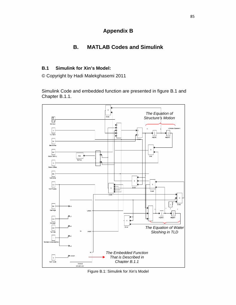
85
Appendix B
B. MATLAB Codes and Simulink
B.1 Simulink for Xin’s Model: © Copyright by Hadi Malekghasemi 2011 Simulink Code and embedded function are presented in figure B.1 and Chapter B.1.1.
Figure B.1: Simulink for Xin’s Model
The Equation of Water Sloshing in TLD
The Equation of Structure’s Motion
The Embedded Function That is Described in
Chapter B.1.1
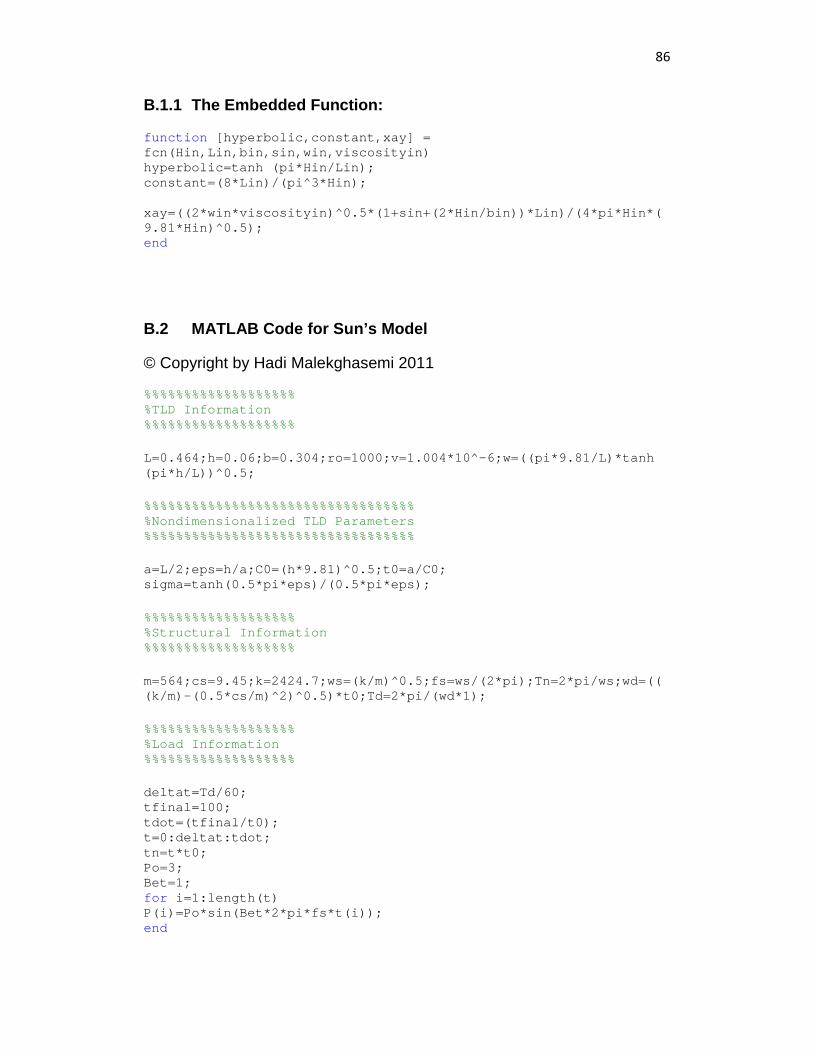
86
B.1.1 The Embedded Function:
function [hyperbolic,constant,xay] = fcn(Hin,Lin,bin,sin,win,viscosityin) hyperbolic=tanh (pi*Hin/Lin); constant=(8*Lin)/(pi^3*Hin); xay=((2*win*viscosityin)^0.5*(1+sin+(2*Hin/bin))*Lin)/(4*pi*Hin*(9.81*Hin)^0.5); end
B.2 MATLAB Code for Sun’s Model
© Copyright by Hadi Malekghasemi 2011 %%%%%%%%%%%%%%%%%%% %TLD Information %%%%%%%%%%%%%%%%%%% L=0.464;h=0.06;b=0.304;ro=1000;v=1.004*10^-6;w=((pi*9.81/L)*tanh (pi*h/L))^0.5; %%%%%%%%%%%%%%%%%%%%%%%%%%%%%%%%%% %Nondimensionalized TLD Parameters %%%%%%%%%%%%%%%%%%%%%%%%%%%%%%%%%% a=L/2;eps=h/a;C0=(h*9.81)^0.5;t0=a/C0; sigma=tanh(0.5*pi*eps)/(0.5*pi*eps); %%%%%%%%%%%%%%%%%%% %Structural Information %%%%%%%%%%%%%%%%%%% m=564;cs=9.45;k=2424.7;ws=(k/m)^0.5;fs=ws/(2*pi);Tn=2*pi/ws;wd=(((k/m)-(0.5*cs/m)^2)^0.5)*t0;Td=2*pi/(wd*1); %%%%%%%%%%%%%%%%%%% %Load Information %%%%%%%%%%%%%%%%%%% deltat=Td/60; tfinal=100; tdot=(tfinal/t0); t=0:deltat:tdot; tn=t*t0; Po=3; Bet=1; for i=1:length(t) P(i)=Po*sin(Bet*2*pi*fs*t(i)); end
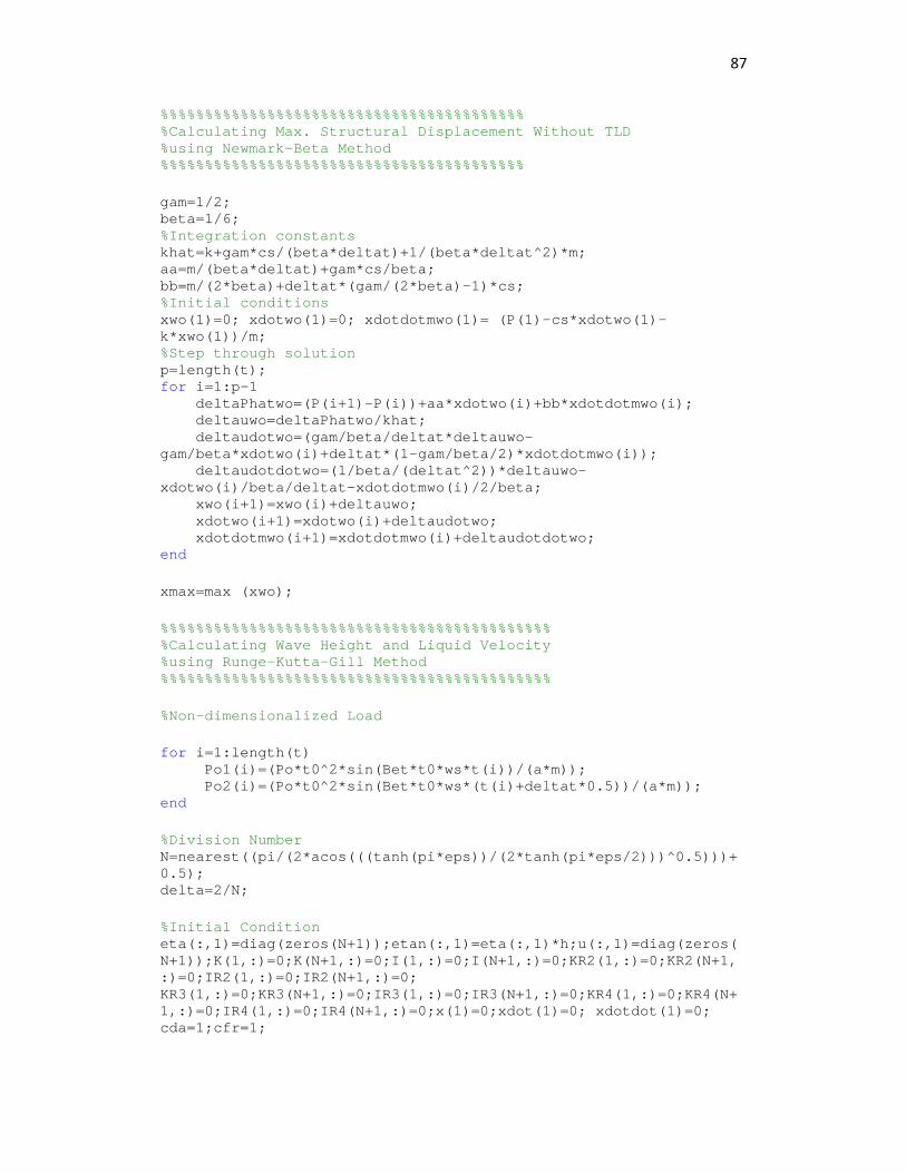
87
%%%%%%%%%%%%%%%%%%%%%%%%%%%%%%%%%%%%%%%%% %Calculating Max. Structural Displacement Without TLD %using Newmark-Beta Method %%%%%%%%%%%%%%%%%%%%%%%%%%%%%%%%%%%%%%%%% gam=1/2; beta=1/6; %Integration constants khat=k+gam*cs/(beta*deltat)+1/(beta*deltat^2)*m; aa=m/(beta*deltat)+gam*cs/beta; bb=m/(2*beta)+deltat*(gam/(2*beta)-1)*cs; %Initial conditions xwo(1)=0; xdotwo(1)=0; xdotdotmwo(1)= (P(1)-cs*xdotwo(1)-k*xwo(1))/m; %Step through solution p=length(t); for i=1:p-1 deltaPhatwo=(P(i+1)-P(i))+aa*xdotwo(i)+bb*xdotdotmwo(i); deltauwo=deltaPhatwo/khat; deltaudotwo=(gam/beta/deltat*deltauwo-gam/beta*xdotwo(i)+deltat*(1-gam/beta/2)*xdotdotmwo(i)); deltaudotdotwo=(1/beta/(deltat^2))*deltauwo-xdotwo(i)/beta/deltat-xdotdotmwo(i)/2/beta; xwo(i+1)=xwo(i)+deltauwo; xdotwo(i+1)=xdotwo(i)+deltaudotwo; xdotdotmwo(i+1)=xdotdotmwo(i)+deltaudotdotwo; end xmax=max (xwo); %%%%%%%%%%%%%%%%%%%%%%%%%%%%%%%%%%%%%%%%%%%% %Calculating Wave Height and Liquid Velocity %using Runge-Kutta-Gill Method %%%%%%%%%%%%%%%%%%%%%%%%%%%%%%%%%%%%%%%%%%%% %Non-dimensionalized Load for i=1:length(t) Po1(i)=(Po*t0^2*sin(Bet*t0*ws*t(i))/(a*m)); Po2(i)=(Po*t0^2*sin(Bet*t0*ws*(t(i)+deltat*0.5))/(a*m)); end %Division Number N=nearest((pi/(2*acos(((tanh(pi*eps))/(2*tanh(pi*eps/2)))^0.5)))+0.5); delta=2/N; %Initial Condition eta(:,1)=diag(zeros(N+1));etan(:,1)=eta(:,1)*h;u(:,1)=diag(zeros(N+1));K(1,:)=0;K(N+1,:)=0;I(1,:)=0;I(N+1,:)=0;KR2(1,:)=0;KR2(N+1,:)=0;IR2(1,:)=0;IR2(N+1,:)=0; KR3(1,:)=0;KR3(N+1,:)=0;IR3(1,:)=0;IR3(N+1,:)=0;KR4(1,:)=0;KR4(N+1,:)=0;IR4(1,:)=0;IR4(N+1,:)=0;x(1)=0;xdot(1)=0; xdotdot(1)=0; cda=1;cfr=1;
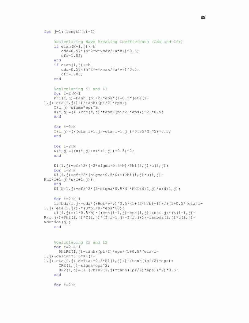
88
for j=1:(length(t)-1) %calculating Wave Breaking Coefficients (Cda and Cfr) if etan(N+1,j)>=h cda=0.57*(h^2*w*xmax/(a*v))^0.5; cfr=1.05; end if etan(1,j)>=h cda=0.57*(h^2*w*xmax/(a*v))^0.5; cfr=1.05; end %calculating K1 and L1 for i=2:N+1 Phi(i,j)=tanh((pi/2)*eps*(1+0.5*(eta(i-1,j)+eta(i,j))))/tanh((pi/2)*eps); C(i,j)=sigma*eps^2; H(i,j)=(1-(Phi(i,j)*tanh((pi/2)*eps))^2)*0.5; end for i=2:N I(i,j)=(((eta(i+1,j)-eta(i-1,j))*0.25*N)^2)*0.5; end for i=2:N K(i,j)=((u(i,j)+u(i+1,j))*0.5)^2; end K1(1,j)=cfr^2*(-2*sigma*0.5*N)*Phi(2,j)*u(2,j); for i=2:N K1(i,j)=cfr^2*(sigma*0.5*N)*(Phi(i,j)*u(i,j)-Phi(i+1,j)*u(i+1,j)); end K1(N+1,j)=cfr^2*(2*sigma*0.5*N)*Phi(N+1,j)*u(N+1,j); for i=2:N+1 lambda(i,j)=cda*((Bet*w*v)^0.5*(1+(2*h/b)+1))/((1+0.5*(eta(i-1,j)-eta(i,j)))*(3*pi/8)*eps*C0); L1(i,j)=(1*0.5*N)*((eta(i-1,j)-eta(i,j))+H(i,j)*(K(i-1,j)-K(i,j))+Phi(i,j)*C(i,j)*(I(i-1,j)-I(i,j)))-lambda(i,j)*u(i,j)-xdotdot(j); end %calculating K2 and L2 for i=2:N+1 PhiR2(i,j)=tanh((pi/2)*eps*(1+0.5*(eta(i-1,j)+deltat*0.5*K1(i-1,j)+eta(i,j)+deltat*0.5*K1(i,j))))/tanh((pi/2)*eps); CR2(i,j)=sigma*eps^2; HR2(i,j)=(1-(PhiR2(i,j)*tanh((pi/2)*eps))^2)*0.5; end for i=2:N
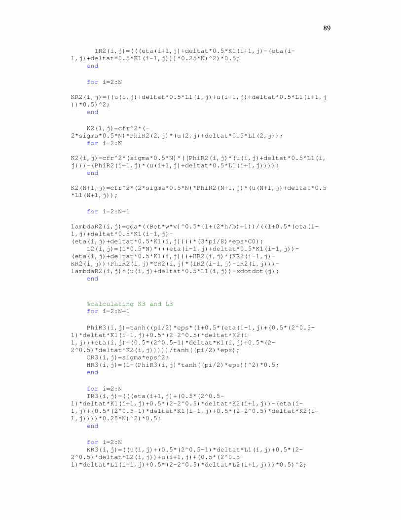
89
IR2(i,j)=(((eta(i+1,j)+deltat*0.5*K1(i+1,j)-(eta(i-1,j)+deltat*0.5*K1(i-1,j)))*0.25*N)^2)*0.5; end for i=2:N KR2(i,j)=((u(i,j)+deltat*0.5*L1(i,j)+u(i+1,j)+deltat*0.5*L1(i+1,j))*0.5)^2; end K2(1,j)=cfr^2*(-2*sigma*0.5*N)*PhiR2(2,j)*(u(2,j)+deltat*0.5*L1(2,j)); for i=2:N K2(i,j)=cfr^2*(sigma*0.5*N)*((PhiR2(i,j)*(u(i,j)+deltat*0.5*L1(i,j)))-(PhiR2(i+1,j)*(u(i+1,j)+deltat*0.5*L1(i+1,j)))); end K2(N+1,j)=cfr^2*(2*sigma*0.5*N)*PhiR2(N+1,j)*(u(N+1,j)+deltat*0.5*L1(N+1,j)); for i=2:N+1 lambdaR2(i,j)=cda*((Bet*w*v)^0.5*(1+(2*h/b)+1))/((1+0.5*(eta(i-1,j)+deltat*0.5*K1(i-1,j)-(eta(i,j)+deltat*0.5*K1(i,j))))*(3*pi/8)*eps*C0); L2(i,j)=(1*0.5*N)*(((eta(i-1,j)+deltat*0.5*K1(i-1,j))-(eta(i,j)+deltat*0.5*K1(i,j)))+HR2(i,j)*(KR2(i-1,j)-KR2(i,j))+PhiR2(i,j)*CR2(i,j)*(IR2(i-1,j)-IR2(i,j)))-lambdaR2(i,j)*(u(i,j)+deltat*0.5*L1(i,j))-xdotdot(j); end %calculating K3 and L3 for i=2:N+1 PhiR3(i,j)=tanh((pi/2)*eps*(1+0.5*(eta(i-1,j)+(0.5*(2^0.5-1)*deltat*K1(i-1,j)+0.5*(2-2^0.5)*deltat*K2(i-1,j))+eta(i,j)+(0.5*(2^0.5-1)*deltat*K1(i,j)+0.5*(2-2^0.5)*deltat*K2(i,j)))))/tanh((pi/2)*eps); CR3(i,j)=sigma*eps^2; HR3(i,j)=(1-(PhiR3(i,j)*tanh((pi/2)*eps))^2)*0.5; end for i=2:N IR3(i,j)=(((eta(i+1,j)+(0.5*(2^0.5-1)*deltat*K1(i+1,j)+0.5*(2-2^0.5)*deltat*K2(i+1,j))-(eta(i-1,j)+(0.5*(2^0.5-1)*deltat*K1(i-1,j)+0.5*(2-2^0.5)*deltat*K2(i-1,j))))*0.25*N)^2)*0.5; end for i=2:N KR3(i,j)=((u(i,j)+(0.5*(2^0.5-1)*deltat*L1(i,j)+0.5*(2-2^0.5)*deltat*L2(i,j))+u(i+1,j)+(0.5*(2^0.5-1)*deltat*L1(i+1,j)+0.5*(2-2^0.5)*deltat*L2(i+1,j)))*0.5)^2;
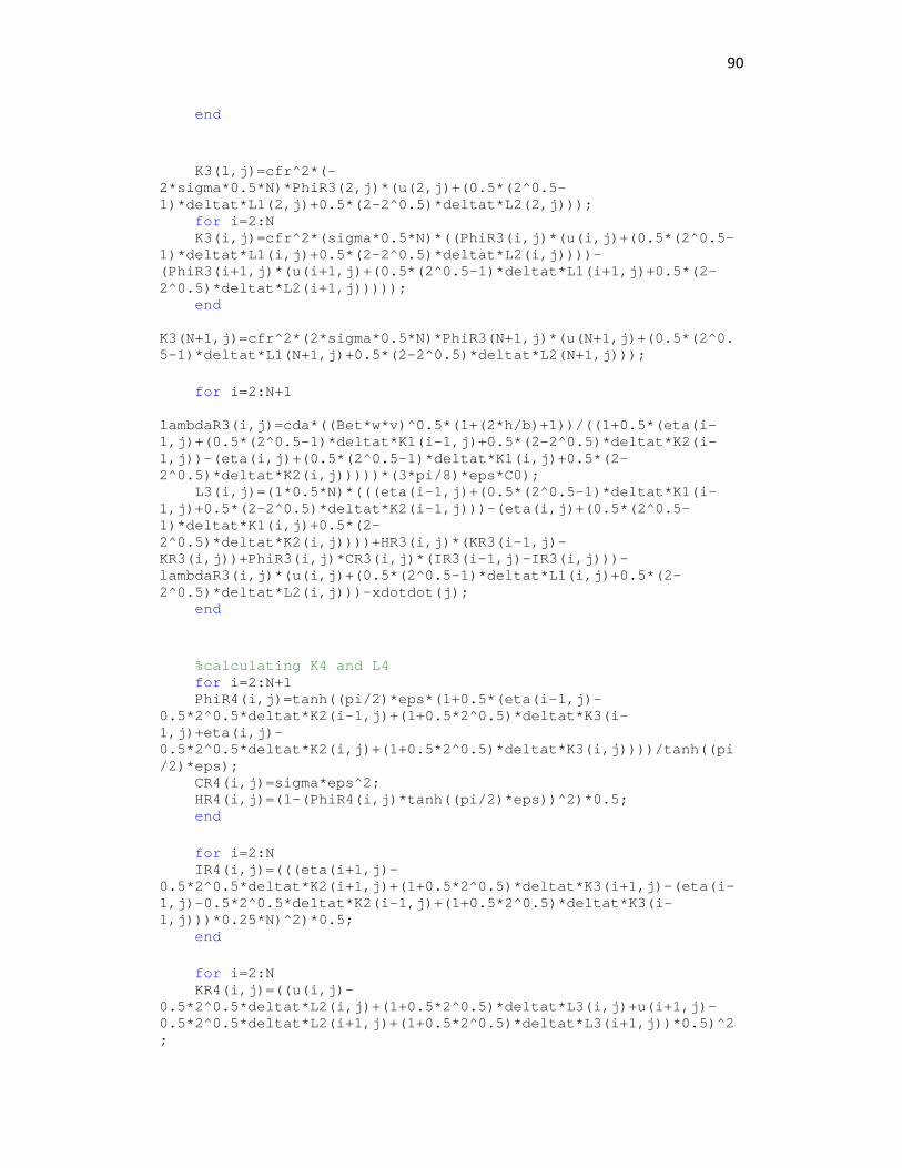
90
end K3(1,j)=cfr^2*(-2*sigma*0.5*N)*PhiR3(2,j)*(u(2,j)+(0.5*(2^0.5-1)*deltat*L1(2,j)+0.5*(2-2^0.5)*deltat*L2(2,j))); for i=2:N K3(i,j)=cfr^2*(sigma*0.5*N)*((PhiR3(i,j)*(u(i,j)+(0.5*(2^0.5-1)*deltat*L1(i,j)+0.5*(2-2^0.5)*deltat*L2(i,j))))-(PhiR3(i+1,j)*(u(i+1,j)+(0.5*(2^0.5-1)*deltat*L1(i+1,j)+0.5*(2-2^0.5)*deltat*L2(i+1,j))))); end K3(N+1,j)=cfr^2*(2*sigma*0.5*N)*PhiR3(N+1,j)*(u(N+1,j)+(0.5*(2^0.5-1)*deltat*L1(N+1,j)+0.5*(2-2^0.5)*deltat*L2(N+1,j))); for i=2:N+1 lambdaR3(i,j)=cda*((Bet*w*v)^0.5*(1+(2*h/b)+1))/((1+0.5*(eta(i-1,j)+(0.5*(2^0.5-1)*deltat*K1(i-1,j)+0.5*(2-2^0.5)*deltat*K2(i-1,j))-(eta(i,j)+(0.5*(2^0.5-1)*deltat*K1(i,j)+0.5*(2-2^0.5)*deltat*K2(i,j)))))*(3*pi/8)*eps*C0); L3(i,j)=(1*0.5*N)*(((eta(i-1,j)+(0.5*(2^0.5-1)*deltat*K1(i-1,j)+0.5*(2-2^0.5)*deltat*K2(i-1,j)))-(eta(i,j)+(0.5*(2^0.5-1)*deltat*K1(i,j)+0.5*(2-2^0.5)*deltat*K2(i,j))))+HR3(i,j)*(KR3(i-1,j)-KR3(i,j))+PhiR3(i,j)*CR3(i,j)*(IR3(i-1,j)-IR3(i,j)))-lambdaR3(i,j)*(u(i,j)+(0.5*(2^0.5-1)*deltat*L1(i,j)+0.5*(2-2^0.5)*deltat*L2(i,j)))-xdotdot(j); end %calculating K4 and L4 for i=2:N+1 PhiR4(i,j)=tanh((pi/2)*eps*(1+0.5*(eta(i-1,j)-0.5*2^0.5*deltat*K2(i-1,j)+(1+0.5*2^0.5)*deltat*K3(i-1,j)+eta(i,j)-0.5*2^0.5*deltat*K2(i,j)+(1+0.5*2^0.5)*deltat*K3(i,j))))/tanh((pi/2)*eps); CR4(i,j)=sigma*eps^2; HR4(i,j)=(1-(PhiR4(i,j)*tanh((pi/2)*eps))^2)*0.5; end for i=2:N IR4(i,j)=(((eta(i+1,j)-0.5*2^0.5*deltat*K2(i+1,j)+(1+0.5*2^0.5)*deltat*K3(i+1,j)-(eta(i-1,j)-0.5*2^0.5*deltat*K2(i-1,j)+(1+0.5*2^0.5)*deltat*K3(i-1,j)))*0.25*N)^2)*0.5; end for i=2:N KR4(i,j)=((u(i,j)-0.5*2^0.5*deltat*L2(i,j)+(1+0.5*2^0.5)*deltat*L3(i,j)+u(i+1,j)-0.5*2^0.5*deltat*L2(i+1,j)+(1+0.5*2^0.5)*deltat*L3(i+1,j))*0.5)^2;
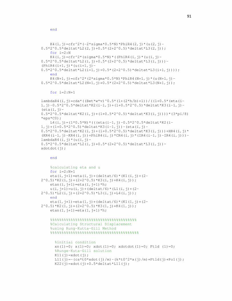
91
end K4(1,j)=cfr^2*(-2*sigma*0.5*N)*PhiR4(2,j)*(u(2,j)-0.5*2^0.5*deltat*L2(2,j)+0.5*(2+2^0.5)*deltat*L3(2,j)); for i=2:N K4(i,j)=cfr^2*(sigma*0.5*N)*((PhiR4(i,j)*(u(i,j)-0.5*2^0.5*deltat*L2(i,j)+0.5*(2+2^0.5)*deltat*L3(i,j)))-(PhiR4(i+1,j)*(u(i+1,j)-0.5*2^0.5*deltat*L2(i+1,j)+0.5*(2+2^0.5)*deltat*L3(i+1,j)))); end K4(N+1,j)=cfr^2*(2*sigma*0.5*N)*PhiR4(N+1,j)*(u(N+1,j)-0.5*2^0.5*deltat*L2(N+1,j)+0.5*(2+2^0.5)*deltat*L3(N+1,j)); for i=2:N+1 lambdaR4(i,j)=cda*((Bet*w*v)^0.5*(1+(2*h/b)+1))/((1+0.5*(eta(i-1,j)-0.5*2^0.5*deltat*K2(i-1,j)+(1+0.5*2^0.5)*deltat*K3(i-1,j)-(eta(i,j)-0.5*2^0.5*deltat*K2(i,j)+(1+0.5*2^0.5)*deltat*K3(i,j))))*(3*pi/8)*eps*C0); L4(i,j)=(1*0.5*N)*(((eta(i-1,j)-0.5*2^0.5*deltat*K2(i-1,j)+(1+0.5*2^0.5)*deltat*K3(i-1,j))-(eta(i,j)-0.5*2^0.5*deltat*K2(i,j)+(1+0.5*2^0.5)*deltat*K3(i,j)))+HR4(i,j)*(KR4(i-1,j)-KR4(i,j))+PhiR4(i,j)*CR4(i,j)*(IR4(i-1,j)-IR4(i,j)))-lambdaR4(i,j)*(u(i,j)-0.5*2^0.5*deltat*L2(i,j)+0.5*(2+2^0.5)*deltat*L3(i,j))-xdotdot(j); end %calculating eta and u for i=2:N+1 eta(i,j+1)=eta(i,j)+(deltat/6)*(K1(i,j)+(2-2^0.5)*K2(i,j)+(2+2^0.5)*K3(i,j)+K4(i,j)); etan(i,j+1)=eta(i,j+1)*h; u(i,j+1)=u(i,j)+(deltat/6)*(L1(i,j)+(2-2^0.5)*L2(i,j)+(2+2^0.5)*L3(i,j)+L4(i,j)); end eta(1,j+1)=eta(1,j)+(deltat/6)*(K1(1,j)+(2-2^0.5)*K2(1,j)+(2+2^0.5)*K3(1,j)+K4(1,j)); etan(1,j+1)=eta(1,j+1)*h; %%%%%%%%%%%%%%%%%%%%%%%%%%%%%%%%%%%%%% %Calculating Structural Displacement %using Rung-Kutta-Gill Method %%%%%%%%%%%%%%%%%%%%%%%%%%%%%%%%%%%%%%% %initial condition xn(1)=0; x(1)=0; xdot(1)=0; xdotdot(1)=0; Ftld (1)=0; %Runge-Kuta-Gill solution K11(j)=xdot(j); L11(j)=-(cs*t0*xdot(j)/m)-(k*t0^2*x(j)/m)+Ftld(j)+Po1(j); K22(j)=xdot(j)+0.5*deltat*L11(j);
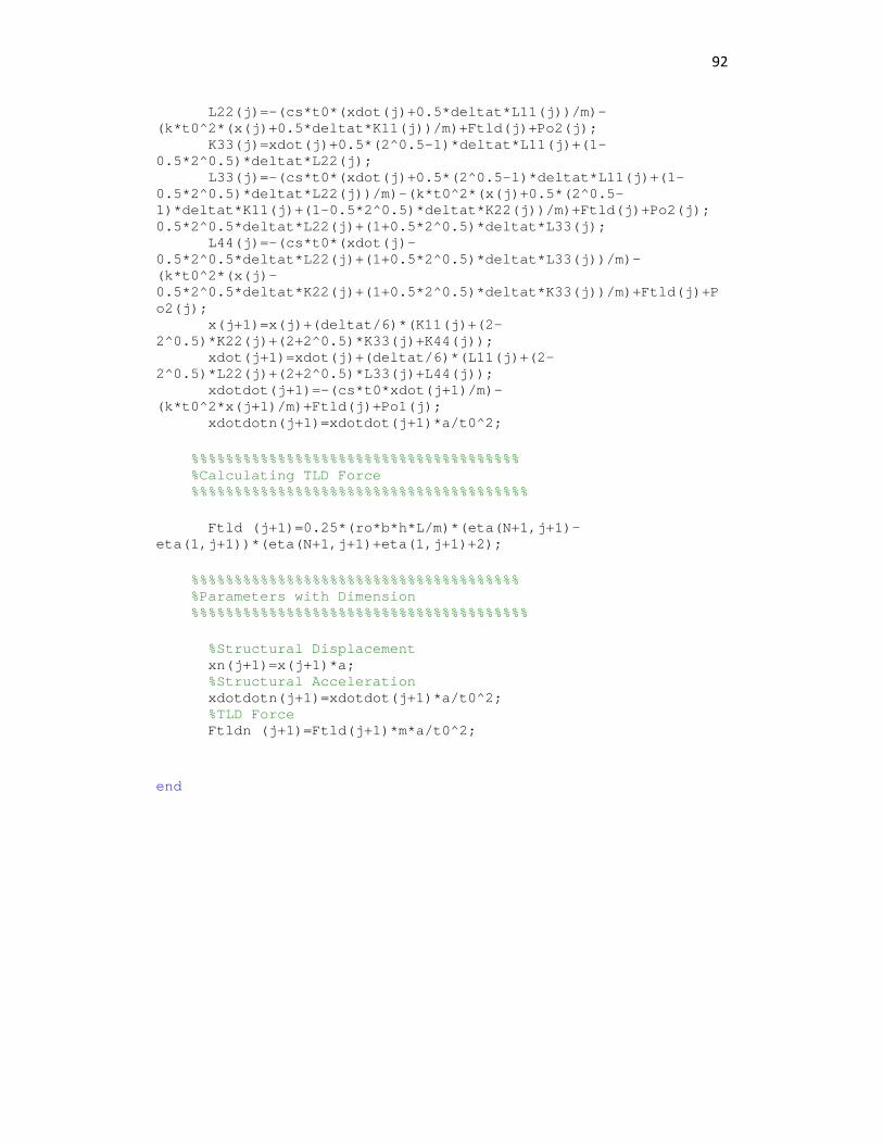
92
L22(j)=-(cs*t0*(xdot(j)+0.5*deltat*L11(j))/m)-(k*t0^2*(x(j)+0.5*deltat*K11(j))/m)+Ftld(j)+Po2(j); K33(j)=xdot(j)+0.5*(2^0.5-1)*deltat*L11(j)+(1-0.5*2^0.5)*deltat*L22(j); L33(j)=-(cs*t0*(xdot(j)+0.5*(2^0.5-1)*deltat*L11(j)+(1-0.5*2^0.5)*deltat*L22(j))/m)-(k*t0^2*(x(j)+0.5*(2^0.5-1)*deltat*K11(j)+(1-0.5*2^0.5)*deltat*K22(j))/m)+Ftld(j)+Po2(j); 0.5*2^0.5*deltat*L22(j)+(1+0.5*2^0.5)*deltat*L33(j); L44(j)=-(cs*t0*(xdot(j)-0.5*2^0.5*deltat*L22(j)+(1+0.5*2^0.5)*deltat*L33(j))/m)-(k*t0^2*(x(j)-0.5*2^0.5*deltat*K22(j)+(1+0.5*2^0.5)*deltat*K33(j))/m)+Ftld(j)+Po2(j); x(j+1)=x(j)+(deltat/6)*(K11(j)+(2-2^0.5)*K22(j)+(2+2^0.5)*K33(j)+K44(j)); xdot(j+1)=xdot(j)+(deltat/6)*(L11(j)+(2-2^0.5)*L22(j)+(2+2^0.5)*L33(j)+L44(j)); xdotdot(j+1)=-(cs*t0*xdot(j+1)/m)-(k*t0^2*x(j+1)/m)+Ftld(j)+Po1(j); xdotdotn(j+1)=xdotdot(j+1)*a/t0^2; %%%%%%%%%%%%%%%%%%%%%%%%%%%%%%%%%%%%%% %Calculating TLD Force %%%%%%%%%%%%%%%%%%%%%%%%%%%%%%%%%%%%%%% Ftld (j+1)=0.25*(ro*b*h*L/m)*(eta(N+1,j+1)-eta(1,j+1))*(eta(N+1,j+1)+eta(1,j+1)+2); %%%%%%%%%%%%%%%%%%%%%%%%%%%%%%%%%%%%%% %Parameters with Dimension %%%%%%%%%%%%%%%%%%%%%%%%%%%%%%%%%%%%%%% %Structural Displacement xn(j+1)=x(j+1)*a; %Structural Acceleration xdotdotn(j+1)=xdotdot(j+1)*a/t0^2; %TLD Force Ftldn (j+1)=Ftld(j+1)*m*a/t0^2; end
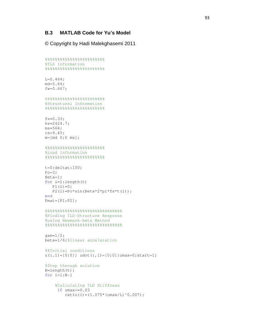
93
B.3 MATLAB Code for Yu’s Model
© Copyright by Hadi Malekghasemi 2011
%%%%%%%%%%%%%%%%%%%%%%%% %TLD Information %%%%%%%%%%%%%%%%%%%%%%%% L=0.464; md=5.64; fw=0.667; %%%%%%%%%%%%%%%%%%%%%%%% %Structural Information %%%%%%%%%%%%%%%%%%%%%%%% fs=0.33; ks=2424.7; ms=564; cs=9.45; m=[md 0;0 ms]; %%%%%%%%%%%%%%%%%%%%%%%% %Load Information %%%%%%%%%%%%%%%%%%%%%%%% t=0:deltat:100; Po=3; Beta=1; for i=1:length(t) P1(i)=0; P2(i)=Po*sin(Beta*2*pi*fs*t(i)); end Pmat=[P1;P2]; %%%%%%%%%%%%%%%%%%%%%%%%%%%%%%% %Finding TLD-Structure Response %using Newmark-beta Method %%%%%%%%%%%%%%%%%%%%%%%%%%%%%%% gam=1/2; beta=1/6;%linear acceleration %%Initial conditions u(:,1)=[0;0]; udot(:,1)=[0;0];umax=0;start=1; %Step through solution N=length(t); for i=1:N-1 %Calculating TLD Stiffness if umax<=0.03 ratio(i)=(1.075*(umax/L)^0.007);
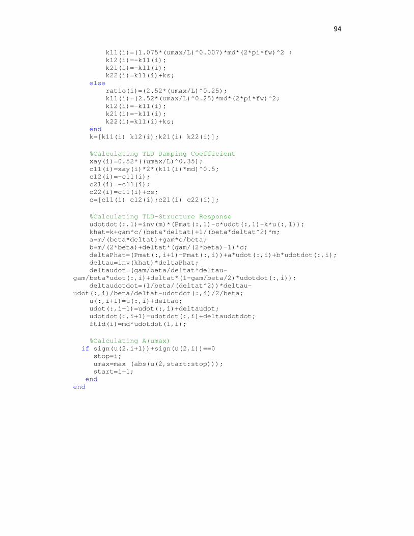
94
k11(i)=(1.075*(umax/L)^0.007)*md*(2*pi*fw)^2 ; k12(i)=-k11(i); k21(i)=-k11(i); k22(i)=k11(i)+ks; else ratio(i)=(2.52*(umax/L)^0.25); k11(i)=(2.52*(umax/L)^0.25)*md*(2*pi*fw)^2; k12(i)=-k11(i); k21(i)=-k11(i); k22(i)=k11(i)+ks; end k=[k11(i) k12(i);k21(i) k22(i)]; %Calculating TLD Damping Coefficient xay(i)=0.52*((umax/L)^0.35); c11(i)=xay(i)*2*(k11(i)*md)^0.5; c12(i)=-c11(i); c21(i)=-c11(i); c22(i)=c11(i)+cs; c=[c11(i) c12(i);c21(i) c22(i)]; %Calculating TLD-Structure Response udotdot(:,1)=inv(m)*(Pmat(:,1)-c*udot(:,1)-k*u(:,1)); khat=k+gam*c/(beta*deltat)+1/(beta*deltat^2)*m; a=m/(beta*deltat)+gam*c/beta; b=m/(2*beta)+deltat*(gam/(2*beta)-1)*c; deltaPhat=(Pmat(:,i+1)-Pmat(:,i))+a*udot(:,i)+b*udotdot(:,i); deltau=inv(khat)*deltaPhat; deltaudot=(gam/beta/deltat*deltau-gam/beta*udot(:,i)+deltat*(1-gam/beta/2)*udotdot(:,i)); deltaudotdot=(1/beta/(deltat^2))*deltau-udot(:,i)/beta/deltat-udotdot(:,i)/2/beta; u(:,i+1)=u(:,i)+deltau; udot(:,i+1)=udot(:,i)+deltaudot; udotdot(:,i+1)=udotdot(:,i)+deltaudotdot; ftld(i)=md*udotdot(1,i); %Calculating A(umax) if sign(u(2,i+1))+sign(u(2,i))==0 stop=i; umax=max (abs(u(2,start:stop))); start=i+1; end end

95
Appendix C
C. List of Symbols and Acronyms
h: undisturbed water depth
L: wave length
a: half length of the tank
b: tank width
u: liquid velocities in the x direction
w: liquid velocities in the z direction
g: gravity acceleration
p: pressure
ρ: liquid density
v: kinematic viscosity of the liquid
Φ: potential function
k: wave number
η: free surface elevation
ηn : free surface elevations at the right tank wall
η0: free surface elevations at the left tank wall
λ: damping coefficient
ωl: fundamental frequency of the liquid
S: surface contaminating factor
ms : structural mass
cs : structural damping coefficient
96
ks : structural stiffness
ξs : structural damping ratio
ws : structural natural frequency
xs : relative displacement of the structure
xs : relative velocity of the structure
xs : relative acceleration of the structure
ag: ground acceleration
F: TLD base shear
kd : stiffness of the NSD model
cd : damping coefficient of the NSD model
md : mass of the NSD model
Ew : energy dissipation per cycle
Ew : non-dimensionalized energy dissipation per cycle
Fw : Liquid sloshing motion force
mw : mass of the liquid
w: excitation angular frequency
A: amplitude of the sinusoidal excitation
Ed : non-dimensional energy dissipation of the NSD model
�Fd�: non-dimensionalized amplitude of the interaction force of the NSD
model
ϕ: phase of the interaction force of the NSD model
β: excitation frequency ratio
fe : excitation frequency
fd : natural frequency of the NSD model
97
ξd : damping ratio of the NSD model
ccr : critical damping coefficient
wd : linear fundamental natural angular frequency of the NSD model
ξ: frequency shift ratio
fw : linear fundamental frequency of the liquid
κ: stiffness hardening ratio
ᴧ: non-dimensional value of the amplitude
L′: equivalent length of the flat-bottom tank
B′: equivalent width of the flat-bottom tank
H′: maximum water depth of the equivalent flat-bottom tank
Vw : total volume of the water
y: first modal acceleration of water sloshing


![ANALYTICAL INVESTIGATIONS ON PROPERTIES OF REACTANTS [H2 - AIR] AND PRODUCTS AT DIFFERENT EQUIVALENCE RATIO](https://img.pdfslide.us/doc/110x75/577cc5891a28aba7119cb87d/analytical-investigations-on-properties-of-reactants-h2-air-and-products.jpg)