Analytical and experimental investigations of dual-plane PIV

Downloaded From: http://spiedigitallibrary.org/ on 09/13/2013 Terms of Use: http://spiedl.org/terms

Analytical and experimental investigations of dual-plane PIV

M. Raffel I, J . Westerweel2, C. Willert 1, M . Gharib 3, J. Kompenhans 1

1 DLR, Institut fitr Stromungsmechanik (CQV), BunsenstraSe 10, D-37073 Gottingen, Germany

2 Delft University of Technology, Aero and Hydrodynamics, Rotterdamseweg 145, 2628 AL Delft, the Netherlands

3 CAL TECH, Graduate Aeronautical Laboratory (CQV), Pasadena CA 91125, California, USA

ABSTRACT In its 'classical' form particle image velocimetry (PIV) extracts two components of the flow velocity vector by measuring the displacement of tracer particles within a double-pulsed laser light sheet. The method described in this paper is based on the additional recording of a third exposure of the tracer particles in a parallel light sheet, which is slightly displaced with respect to the first one. The particle images resulting from these three exposures are stored on separate frames. The locations of the correlation peaks, as obtained by cross-correlation methods, are used to determine the projections of the velocity vectors onto the plane between both light sheets. In the manner described below, the amplitudes of these peaks are used to obtain information about the velocity component perpendicular to the light sheet planes. The mathematical background of this method is described in the paper. Numerical simulations show the influence of the main parameters (e.g . light sheet thickness, light sheet displacement and out-of-plane component) on the resolution and reliability of the new method. Two different recording procedures and their results will be shown to demonstrate the ease of operation when applying this technique to liquid flows.

KEYWORDS particle image velocimetry, dual-plane correlation, scanning light sheet, three-dimensional flow measurements

1. INTRODUCTION In PIV the velocity vector field is usually determined by subdividing the recordings into interrogation windows and employing particle tracking algorithms or statistical evaluation techniques, such as histogram-analysis, analysis of Young's fringes or other correlation methods. The correlation methods are widely used, as they can easily be implemented into fast, reliable and fully automatic evaluation systems. Their theory is well known and described by various authors (e.g. Adrian (1988), Keane and Adrian (1990, 1992), Hinsch (1993), Westerweel (1993)). The method described in this paper is based on the spatial cross-correlation of particle images stored on separate frames of each exposure as described by Willert and Gharib ( 1991 ). It is expanded by the analysis of the heights of the peaks in the correlation plane. This value depends on the portion of paired particle images, which itself depends on the outof-plane velocity component, but also on other parameters. To circumvent problems with these other influences (e.g. background light, varying image size and number ,loss of pairs due to in-plane motion), images from a displaced light sheet plane, parallel to the first are also recorded for peak height normalization. In the following this concept will be referred to as 'dual-plane correlation technique' or 'dual-plane PIV'. The recording of images of particles within a parallel light sheet on a third frame offers the following advantages: (1) the influence of the loss of image pairs due to the in-plane velocity on the out-of-plane velocity estimation can be reduced by normalization; (2) the directional ambiguity of the out-of-plane velocity component can be removed; (3) a larger out-of-plane velocity component can be tolerated compared to conventional PIV; and (4) a higher signal-to-noise ratio for the out-of-plane velocity estimation can be achieved. These aspects become clearer through the descrition of the ensemble averages in PIV evaluation in section 2 . Additionally, the influence of finite numbers of particle images will be shown by numerical simulations in section 3.

2. PROOF OF CONCEPT The dual-plane correlation technique considers three images lo(x,y), l1(x,y), and l2(x,y) of tracer particles suspended in a fluid recorded at t0, tb and t2 respectively, with: trto, = t2-t1, = l:l.t. The particles are illuminated by light sheets

0-8 7 94-7 905-2/95/$6.00 SP/E Vol. 2546 I 75


that are parallel to the image plane.The intensity proftles in the direction perpendicular to the image plane (Z) are represented by lo(Z), I 1(Z), and J2(Z) respectively. The shape of these profiles is assumed to be identical for all three exposures; the locations of the centers along the Z-direction for lc;(Z), and IJ(Z) are equal (Zo and Z1 respectively), whereas the center of J2(Z) is shifted over a distance Z2-Z 1 , i.e.1:

lo(Z) = I 1(Z) = I(Z) and (1)

The tracer particles suspended in the fluid can be described by:

G(X,t) = L 5[ X- Xn(t)] (2) n

where 5(X) is the Dirac 5-function, and xn (t) is the location of the tracer particle with index n at time t. The

coordinates X and Y of the vector X= (X,Y,Z,) are parallel to the image coordinates x andy respectively; the Z

coordinate is perpendicular to the image plane. (Note that the integral of G(X,r) over a volume V yields the number

of particles in V). The realizations for the images Io(x,y), lt(x,y), -and l2(x,y) correspond to G(X,t) at to, tb and t2

respectively, or:

(3)

The displacement vector D is considered uniform and constant over each time intervalllt. 2 Hence,

(4)

The image Iifx ,y), and the tracer pattern G; (X) are related by:

I ;(x,y) =I, ·t(x,y)® g;(x,y) (5)

where ® denotes the (two-dimensional) convolution integral, and where lz is the maximum of I(Z), t(x,y) the normalized intensity distribution of a single particle image, and g,{x,y) the projection of G;(X), weighted by l,{Z)

onto the image plane, i.e.:

8;(x,y) =..!. J f;(Z)G;(x I M,y I M,Z)dz I,

(6)

where M is the magnificationl. (Note that the integral of g,{x,y) over an area A yields the (non-integer) number of particle images in A.)

The particles are distributed randomly over the fluid. It is therefore more convenient to deal with the images and tracer particles in terms of random fields. The cross-covariance of Jo(x,y), and lt(x,y) taken over the ensemble of all realizations for Xn(t0 ) for all n is defined as:

(7)

1 In a later expansion of this technique an additional shift between z0 and Z 1 can be introduced to allow out-of-plane velocity components in both directions (see section 5). 2Tbis condition is usually satisfied locally. 3 A parallel projection instead of a perspective projection is assumed here.

76 I SPIE Vol. 2546


where { ... ) denotes the ensemble averaging; vice versa for the cross-covariance of I 1(x,y), and l2(x,y).

The cross-covariance of G0 (X) with G1(X) taken over the ensemble of all realizations for Xn (t0 ) for all n is defined as:

(8)

cf. (7); vice versa for the cross-covariance of G1(X) , and G2(X). If the tracer particles are ideal and distributed

homogeneously over the fluid, and the displacement i5 is uniform and constant, then:

(9)

where C is the number density of the tracer particles, and S is the three-dimensional separation vector. (Note that

C = (G;(X)).>

Substitution of (5) in (7), using (6), and substituting the relations (1) and (9) yields (detailed derivation see Westerweel (1993)):

R1•1, (r, s) = R1olo (r - MDx ,s - MDr )· F0 (Dz)

R1,1, (r,s) = Rr.1• (r-MDx ,s-MDy)-F0 (Dz -Z2 + Z1)

J I (Z )I (Z+Dz)dZ E(D ) =~~---~----o z J {J(z )}2 dZ

(10)

with:

(11)

where Riolo (r ,s) is the ensemble auto-covariance of I o(x ,y) and i5 = (Dx,Dr ,Dz)· Note that R~o1, (r,s) and R1,1, (r,s)

are identical to Riolo (r ,s) shifted over the in-plane displacement and scaled by the out-of-plane correlation. Taking

the ratio of R, 1 (r, s) and R11 (r, s) yields (for brevity of notation the coordinates rands were omitted): -<1 I I 2

(12)

This is the solution for determining Dz for an arbitrary intensity profile of the light sheets and a given shift Z2-Z1 . In fact, this equation can be seen as a kind of lookup table; note that there is only a solution for Dz where F o(Z) is 'uniquely invertible'.4

Since most CW-lasers offer a sufficient beam-pointing stability, their intensity profiles can easily be determined to find the exact relation between the out-of-plane velocity and the aoss-covariance values. When using solid state pulse laser systems- as for example Nd:YAG laser systems - a pulse-to-pulse beam-pointing stability of up to 20% of the beam diameter has to be taken into account. In this case, the intensity profile should be determined simultaneously e .g . by using a beam splitter and a video array. However to keep explanation and computation simple we assumed a light sheet with a top-hat intensity profile, i .e .

I (Z) = {/ z IZI s: ~ /2 0 elsewhere

we.have: (13)

41his implies that we can only use one half ofF o(Z). In other words, for accurate measurement of w it needs to be away from regions where the inverse ofFo(Z) is steep. This implies that we cannot accurately measure small win a Gaussian light sheet.

SPIE Vol. 2546 I 77


IZI ~IlZ elsewhere

where .1Z is the width of the light sheet. Now substitute (14) in (12) and solve the equation for 0 ~ D2 ~ Z2 - 21:

Dz = !lZ R1,1, / R~. -1+(22 -21)/ llZ

RI,I2 I R~. + 1

Substitution of D2 = wAt, where w is the out-of-plane velocity and Oz=l -(Z2-Z1)1!lZyields:

cf. Raffel et.al. (1995).

3. SIMULATIONS

(14)

(15)

(16)

When using the same software as for the dual frame cross-correlation analysis, and therefore the same peak-flnding algorithm for both evaluations, both displacements need to be valid for reconstruction of the out-of-plane velocity component. The valid data yield for an image frame pair is proportional to the image density reduced by the in-plane loss of pairs and the out-of-plane loss of pairs N1 F1 F 0 · Wherein F o = (1 - !Dlil !lZ) is the out-of-plane loss of pairs for the flrst and second image frames, and F 0 = (Oz + !D7ll!:lZ) the out-of-plane loss of pairs for the second and third image frames. Note that reducing /Dz/ will improve the valid data yield for the first and second image frames, but at the same time reduce the valid data yield for the second and third image frames. Therefore it is necessary to determine the optimum situation in which the data yield for each corresponding correlation pair is maximal. Also, it is necessary to determine for which set of parameters the measurement errors are minimal. For this purpose a number of simulations were carried out. The parameter sets that were simulated are listed in table 1. The total number of parameter combinations is equal to 349; for each combination a triplet of digital image frames is generated. For simplification the in-plane displacement was assumed to have only a X -component.

0.0 0.2 0.4 0.6 0.8 15 20 0.0 0.1 0.2 0.4 0.0 0.1 0.2 0.3 0.4 0.5 0.6 0.7 0.8 0.9 1.0

Table 1 Overview of the parameter sets that were simulated.

For each simulation a set of random particle locations is generated within a rectangular volume, where the number density of the particles matched a given image density (N1). Each particle was assigned a 'brightness value,' determined by its location within the light sheet; subsequently, a 512 by 512 pixels digital image frame is computed for the given particle locations and their assigned brightness values. A Gaussian intensity distribution with an e-2_ width of 1.2 pixels is assumed for each particle image; the actual pixel value is found by integration of a twodimensional Gaussian intensity distribution over the area of each pixel (integrals of a Gaussian distribution can be expressed conveniently as error functions). For the second and third image the particle locations are uniformly translated over a predefined displacement prior to computing the image frame. For the first and second images the location of the light sheet remains unchanged, whereas for the third image the location of the light sheet is adjusted according to the value for the image overlap (Oz). i .e.: (1-0z) !:lZ. The light sheet intensity profile is uniform within a width !lZ and is equal to 1; the diameter of an interrogation area (in simulation units) is also taken equal to 1. For each triplet, the firSt and second images and the second and third images are analyzed using the cross-correlation method. This yields two data sets that consist of the location of the displacement-correlation peak and its height for each interrogation position. Each interrogation is done over areas of 32 by 32 pixels with a 50% overlap between adjacent interrogation areas. So, the total number of interrogations per image is 961 (of which only 256 are truly independent). Despite the high image density, there remains a finite probability for the occurrence of spurious displacements. To detect spurious vectors, each displacement vector is compared to the known displacement, and all

78 I SPIE Vol. 2546


vectors that deviate by more than 0.5 pixel from the true value are discarded from the data set. (Only for simulated data - where the actual displacement is known - it is possible to use such a strict selection criterion). The remaining data from the two data sets are used to reconstruct the out-of-plane component of the displacement.

3.1. RESULTS OF SIMULATION The success rate (or valid data yield), denoted as r, depends on the image density (NJ). the in-plane displacement (Dx). and the out-of-plane displacement (Dz). Ifr is plotted against the product of N1 F1 F o (Keane & Adrian 1990) then all data practically collapses onto a single curve, as shown in Figure 1. 11lis curve corresponds to the probability curve for the presence of at least four particle images per interrogation area, given that the number of particle images has a Poisson distribution (Westerweel1993).

1.0

0.8

0.6

'-0.4 [

I o.2 r g I

r 0.0

0 5 10

~ ::: ~-· 0.4 ~~ ; · ~ =0.0

-o.z 0 ·-· 0.4

•2 • ~0.6

o.o f/ o-o 0.8

-0.4 -0.2 0

15 20 NIF,Fo

N1 = 15 F, = 1. 0

0., . 0.4 Dz I t::.Z- (1-0 2 ) I 2

Fig. I: The valid data yield (r) as a function of the ef!etive number of particle images (Nl F1 F o). The solid line represents the probability for having at least four particle images.

Fig. 2: The valid data yield of the reconstructed displacements rr rec> as a function of the out-ofplane displacement (D7) with respect to the center of the overlap region of the light-sheets (05 (1-0z) A Z) for different values ol 0 z with F1 = 1 and N1 = 15.

The fraction where both interrogations were valid is given by the product of the valid data yield for the first and second images (r 01) and the valid data yield for the second and third images (r ~:z>; the correlation coefficient between the total combined valid data yield and the product of r 01 and r 12 is equal to 0.99994. Figure 2 shows the valid data yield of the reconstructed displacement vectors as a function of the out-of-plane displacement (Dz) with respect to the center of the light-sheet overlap region (i.e. 05 ( 1-0z) tu:). This graph only shows the results from the simulations with F1 = 1 (i.e. DxlllX = 0.0) and N1 = 15; the results for other values of F1 and N1 are similar. A substantial valid data yield (i.e. r > 0.75) is only found for:

/Dzll:l Z - 05 (1 -0z) A Z/ < 0.25. (17)

SPIE Vol. 2546 I 79


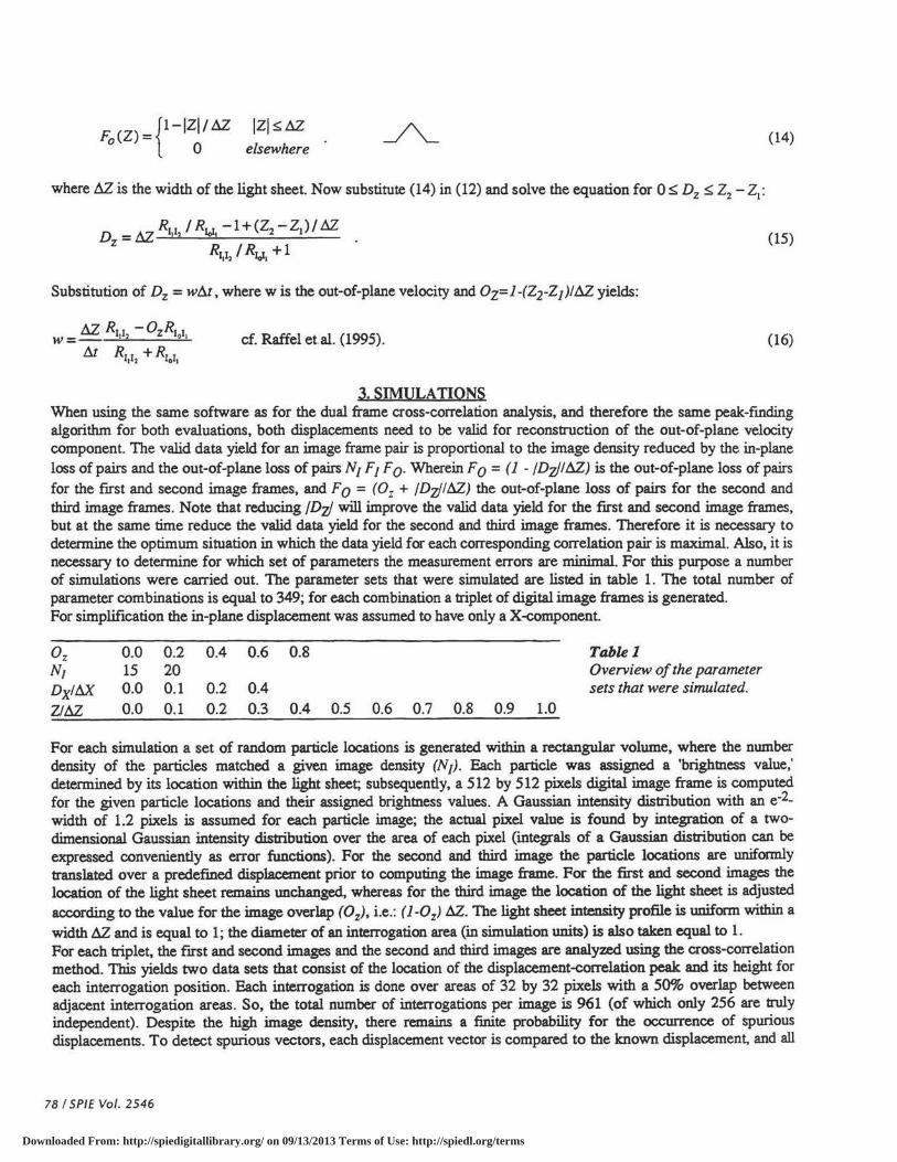
In Figure 3 the results for the RMS error for the in-plane displacement as a function of the out-of-plane displacement are plotted for different in-plane displacements with Oz = 0.0. (Graphs for other values of Oz show the same qualitative behavior.) 1b.is graph shows that the RMS error for the measured in-plane displacement is lowest for Dx = 0, which complies with earlier results by Willert & Gbarib (1991) and Westerweel (1993). Also note how the error becomes almost zero for Dzl tlZ = 0.5; this will be discussed further below. Since we are dealing with crosscorrelation analysis of pairs of single-exposure image frames it is always possible to shift the interrogation images in the two image frames with respect to each other in such a manner that the effec~ve particle-image displacement is equal to zero. We therefore consider only the case for Dx = 0 in the remainder ~of the discussion of the simulation results.

f '

Dx i 6X = .... o.o

N1 = 15 Oz = 0. 0

0.0 .._. _ __.. __ ___.___.. ___ ____.

o.o 0.2 0.4 o.6 o.s 1.0 Dz I 6Z

0.2 r-, ---------~ ' • r •

~ 0.1 I : -.. • I I

N t . ! Q 0 !-- •···-1-···e---t-··1·-·---; ;::._ t Oz = : • ' eN t • o.o • • I ~ -0.1 ~ : ~~ = I

r • o.6 , t 0 0.8 :

-0.2 -0.4 -0.2 0.0 0.1 0.4

~ =1.0

Dz I 62 - (1- Oz ) I 2

Fig. 3: The results for the RMS error for the in-plane displacement as a function of the out-of-plane displacement for different in-plane displacements with N1 = 15 and Oz = 0.0.

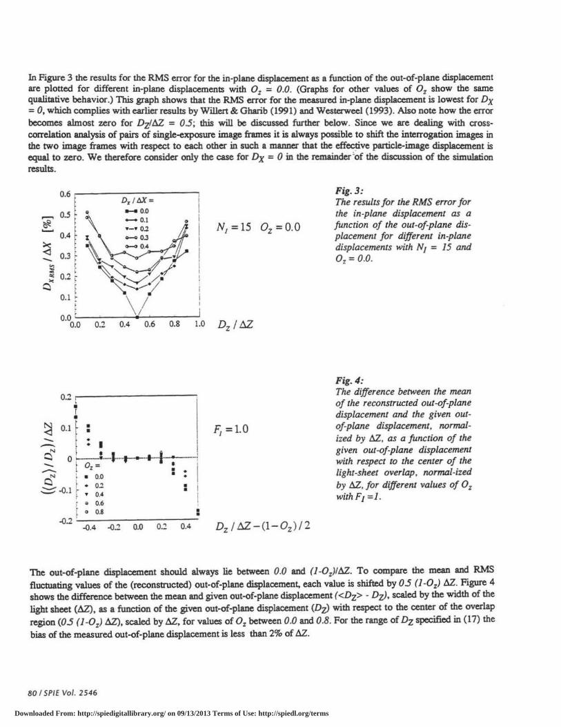
Fig. 4: The difference between the mean of the reconstructed out-of-plane displacement and the given outof-plane displacement, normalized by tlZ. as a function of the given out-of-plane displacement with respect to the center of the light-sheet overlap, normal-ized by tlZ, for different values of 0 z withF1 =I .

The out-of-plane displacement should always lie between 0.0 and {1 -0z)lllZ. To compare the mean and RMS fluctuating values of the (reconstructed) out-of-plane displacement, each value is shifted by 0.5 ( 1-0 z) llZ. Figure 4 shows the difference between the mean and given out-of-plane displacement ( <Dz> - Dz). scaled by the width of the light sheet (tlZ), as a function of the given out-of-plane displacement (Dz) with respect to the center of the overlap

region (0 .5 (1-0 z) tlZ), scaled by tlZ, for values of 0 z between 0.0 and 0.8. For the range of Dz specified in ( 17) the

bias of the measured out-of-plane displacement is less than 2% of llZ.

80 I SPIE Vol. 2546


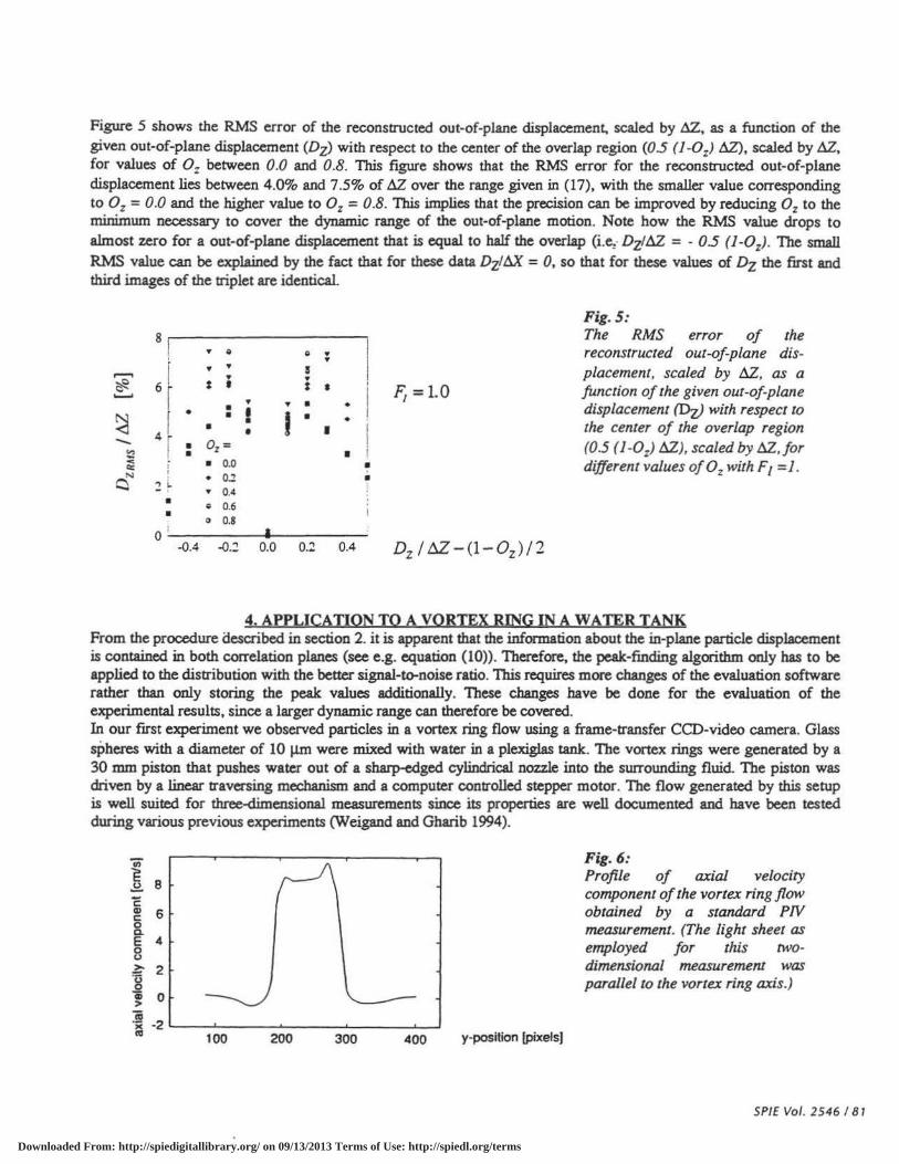
Figure 5 shows the RMS error of the reconstructed out-of-plane displacement, scaled by llZ, as a function of the given out-of-plane displacement (Dz) with respect to the center of the overlap region (OS ( 1-0z) AZ), scaled by AZ, for values of Oz between 0.0 and 0.8. This figure shows that the RMS error for the reconstructed out-of-plane displacement lies between 4.0% and 7.5% of AZ over the range given in (17), with the smaller value corresponding to Oz = 0.0 and the higher value to Oz = 0.8. This implies that the precision can be improved by reducing Oz to the minimum necessary to cover the dynamic range of the out-of-plane motion. Note how the RMS value drops to almost zero for a out-of-plane displacement that is equal to half the overlap (i.e: Dzl AZ = - 0 S ( 1-0 z). The small

RMS value can be explained by the fact that for these data Dzll!.X = 0, so that for these values of Dz the first and third images of the triplet are identical.

Fig. 5:

81 The RMS error of the • g 0 •

I reconstructed out-of-plane dis-

6 f • • • I placement, scaled by AZ, as a r--. • •

~ : • : • I

~ =1.0 junction of the given out-of-plane ~ I • • • • displacement {Dz) with respect to • • I ! ~ 4[ • I • • • • • I I the center of the overlap region - I • Oz= (0.5 {1-0z) AZ), scaled by AZ.jor ~ l • • i < • 0.0 different values of 0 z with F 1 = 1 . co: I • N I

0.2 • Q :! ~ • • 0.4

• ~ 0.6 • 0.8 I)

0 ; -0.4 -0.:! 0.0 0.2 0.4 Dz I DZ -(1-0z)/2

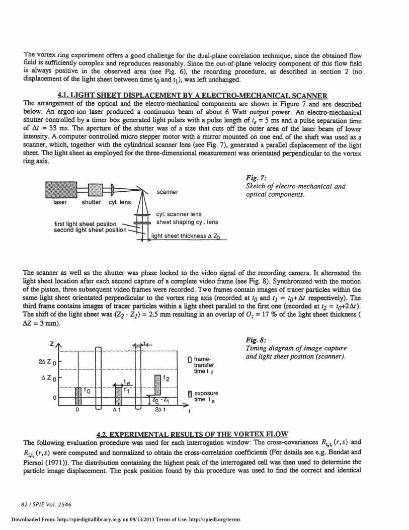
4. APPLICATION TO A VORTEX RING IN A WATER TANK From the procedure aescribed in section 2. it is apparent that the information about the in-plane particle displacement is contained in both correlation planes (see e.g. equation (10)). Therefore, the peak-finding algorithm only has to be applied to the distribution with the better signal-~noise ratio. This requires more changes of the evaluation software rather than only storing the peak values additionally. These changes have be done for the evaluation of the experimental results, since a larger dynamic range can therefore be covered. In our first experiment we observed particles in a vortex ring flow using a frame-transfer CCD-video camera. Glass sPheres with a diameter of 10 ~ were mixed with water in a plexiglas tank. The vortex rings were generated by a 30 mm piston that pushes water out of a sharp-edged cylindrical nozzle into the surrounding fluid. The piston was driven by a linear traversing mechanism and a computer controlled stepper motor. The flow generated by this setup is well suited for three-dimensional measurements since its properties are well documented and have been tested during various previous experiments (Weigand and Gharib 1994).

y-position (pixels)

Fig. 6: Profile of axial velocity component of the vortex ring flow obtained by a standard PJV measurement. (The light sheet as employed for this twodimensional measurement was parallel to the vortex ring axis.)

SPIE Vol. 2546 I 8 7


The vortex ring experiment offers a good challenge for the dual-plane correlation technique. since the obtained flow field is sufficiently complex and reproduces reasonably. Since the out-of-plane velocity component of this flow field is always positive in the observed area (see Fig. 6), the recording procedure. as described in section 2 (no displacement of the light sheet between time to and t1), was left unchanged.

4.1. LIGHT SHEET DISPLACEMENT BY A ELECTRO-MECHANICAL SCANNER The arrangement of the optical and the electro-mechanical components are shown in Figure 7 and are described below. An argon-ion laser produced a continuous beam of about 6 Watt ouq)ut power. An electro-mechanical shutter controlled by a timer box generated light pulses with a pulse length of te = 5 ms and a pulse separation time of & = 33 ms. The aperture of the shutter was of a size that cuts off the outer area of the laser beam of lower intensity. A computer controlled micro stepper motor with a mirror mounted on one end of the shaft was used as a scanner. which, together with the cylindrical scanner lens (see Fig. 7), generated a parallel displacement of the light sheet. The light sheet as employed for the three-dimensional measurement was orientated perpendicular to the vortex ring axis.

first light sheet positon second light sheet position

scanner

cyl. scanner lens sheet shaping cyl. lens

sheet thickness 1!.

Fig. 7: Sketch of electro-mechanical and optical components.

The scanner as well as the shutter was phase locked to the video signal of the recording camera. It alternated the light sheet location after each second capture of a complete video frame (see Fig. 8). Synchronized with the motion of the piston. three subsequent video frames were recorded. Two frames contain images of tracer particles within the same light sheet orientated perpendicular to the vortex ring axis (recorded at to and r1 = to+& respectively). The third frame contains images of tracer particles within a light sheet parallel to the first one (recorded at t2 = to+2&). The shift of the light sheet was (Z2 - Z 1) = 2.5 nun resulting in an overlap of 0 z = 17 % of the light sheet thickness ( llZ = 3 nun).

Q frame· transfer timet f

[J exposure tJme te

Fig. 8: Timing diagram of image capture and light sheer position (scanner).

4.2. EXPERIMENTAL RESULTS OF THE VORTEX FLOW The following evaluation procedure was used for each interrogation window: The cross-covariances R~.,1, (r, s) and

R1,1, (r,s) were computed and normalized to obtain the cross-correlation coefficients (For details see e.g. Bendat and

Piersol (1971)). The distribution containing the highest peak of the interrogated cell was then used to determine the particle image displacement. The peak position found by this procedure was used to find the correct and identical

82 I SPIE Vo l. 2546


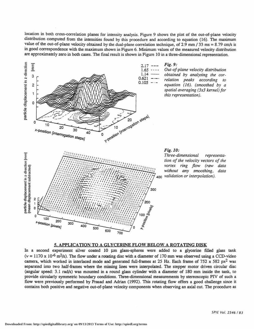
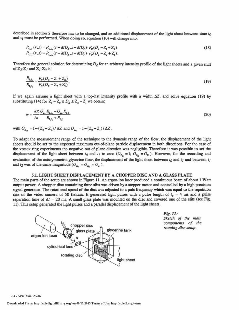
location in both cross-correlation planes for intensity analysis. Figure 9 shows the plot of the out-of-plane velocity distribution computed from the intensities found by this procedure and according to equation (16). The maximum value of the out-of-plane velocity obtained by the dual-plane correlation technique, of 2.9 nun I 33 ms = 8 .79 crn/s is in good correspondence with the maximum shown in Figure 6. Minimum values of the measured velocity distribution are approximately zero in both cases. The fmal result is shown in Figure 10 in a three-dimensional representation.

20 X~~ 30

on ftnten..... . 40 --· "'liation steps)

2.11 1.65 l.l4

0.621 0.105

Fig. 9: Out-of-plane velocity distribution obtained by analysing the correlation peaks according to equation (16). (smoothed by a spatial averaging (3x3 kernel) for this representation).

Fig.JO: Three-dimensional representation of the velocity vectors of the vortex ring flow (raw data without any smoothing , data validation or interpolation).

5. APPLICATION TO A GLYCERINE FWW BEWW A ROTATING DISK In a second experiment silver coated 10 J.1.m glass-spheres were added to a glycerine filled glass tank (v = 1170 x 10-6 m2/s). The flow under a rotating disc with a diameter of 170 mm was observed using a CCD-video camera, which worked in interlaced mode and generated full-frames at 25 Hz. Each frame of 752 x 582 px2 was separated into two half-frames where the missing lines were interpolated. The stepper motor driven circular disc (angular speed: 3.1 rad/s) was mounted in a round glass cylinder with a diameter of 180 nun inside the tank, to provide circularly symmetric boundary conditions. Three-dimensional measurements by stereoscopic PIV of such a flow were previously performed by Prasad and Adrian (1992). This rotating flow offers a good challenge since it contains both positive and negative out-of-plane velocity components when observing an axial cut. The procedure as

SPIE Vol . 2546 I 83


described in section 2 therefore has to be changed, and an additional displacement of the light sheet between time to and t1 must be performed. When doing so, equation (10) will change into:

R1•1, (r,s)= R"'lo (r-MDx,s-MDy)· F0 (Dz -21 +20 )

R1,12 (r,s) = R1010 (r-MDx,s-MDy)· F0 (Dz - 22 +21).

(18)

Therefore the general solution for determining Dz for an arbitrary intensity profile of the light sheets and a given shift of z2-z 1 and z rZo is:

(19)

If we again assume a light sheet with a top-hat intensity profile with a width llZ, and solve equation (19) by substituting (14) for 21 -20 ~ Dz ~ 22 -21 we obtain:

tu, 0 R -0 R W = z,. 1,12 Z.1 1011

t::J Rl I + R, I I 2 .ao I

(20)

To adapt the measurement range of the technique to the dynamic range of the flow, the displacement of the light sheets should be set to the expected maximum out-of-plane particle displacement in both directions. For the case of the vortex ring experiments the negative out-of-plane direction was negligible. Therefore it was possible to set the displacement of the light sheet between to and t1 to zero (Oz., = 1; Oz.. = Oz ). However, for the recording and

evaluation of the axissymmetric glycerine flow, the displacement of the light sheet between to and t1 and between t1 and t2 was of the same magnitude (Oz., = Oz,, = Oz ).

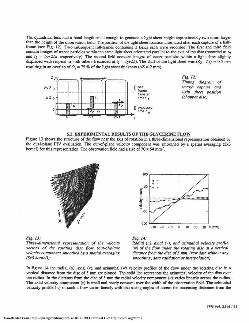
5.1. LIGHT SHEET DISPLACEMENT BY A CHOPPER DISC AND A GLASS PLATE The main parts of the setup are shown in Figure 11. An argon-ion laser produced a continuous beam of about 1 Watt output power. A chopper disc containing three slits was driven by a stepper motor and controlled by a high precision signal generator. The rotational speed of the disc was adjusted to a puis frequency which was equal to the repetition rate of the video camera of 50 fields/s. It generated light pulses with a pulse length of te = 4 ms and a pulse separation time of t::J = 20 ms. A small glass plate was mounted on the disc and covered one of the slits (see Fig. 11). This setup generated the light pulses and a parallel displacement of the light sheets.

84 I SPIE Vol. 2546

Fig.ll: Sketch of the main components of the rotating disc setup.


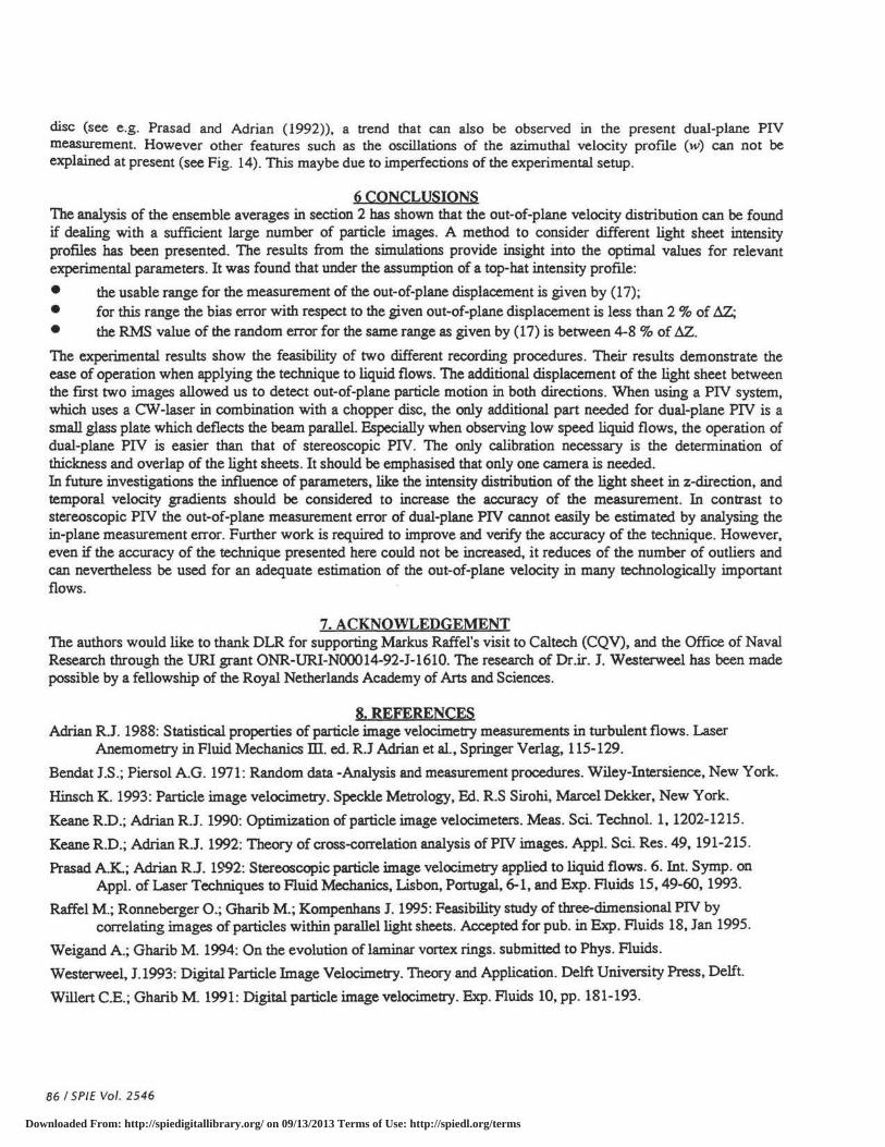
The cylindrical lens had a focal length small enough to generate a light sheet height approximately two times larger than the height of the observation field . The position of the light sheet location alternated after each capture of a halfframe (see Fig. 12). Two subsequent full-frames containing 2 fields each were recorded. The first and third field contain images of tracer particles within the same light sheet orientated parallel to the axis of the disc (recorded at to and t2 = to+2At respectively). The second field contains images of tracer particles within a light sheet slightly displaced with respect to both others (recorded at r1 = to+!lt). The shift of the light sheet was (Z2 - z1) = 0.5 mm resulting in an overlap of 0 z = 75 % of the light sheet thickness (~ = 2 mm).

0 half frametransfer timet f

Fig. 12: Timing diagram of image capture and light sheet position (chopper disc)

5.2. EXPERIMENTAL RESULTS OF THE GLYCERINE FLOW Figure 13 shows the structure of the flow near the axis of rotation in a three-dimensional representation obtained by the dual-plane PIV evaluation. The out-of-plane velocity component was smoothed by a spatial averaging (3x3 kernel) for this representation. The observation field had a size of 70 x 54 mm2.

Fig.13: Three-dimensional representation of the velocity vectors of the rotating disc flow (out-of-plane velocity component smoothed by a spatial averaging (3x3 kernel)).

-30 -20 -10 0 10 20 30 x (mm]

Fig.14: Radial (u) , axial (v), and azimuthal velocity profile (w) of the flow under the rotating disc at a vertical distance from the disc of 5 mm. (raw data without any smoothing, data validation or interpolation).

In figure 14 the radial (u), axial (v), and azimuthal (w) velocity profiles of the flow under the rotating disc in a vertical distance from the disc of 5 mm are plotted. The solid line represents the azimuthal velocity of the disc over the radius. In the distance from the disc of 5 mm the radial velocity component (u) varies linearly across the radius. The axial velocity component (v) is small and nearly constant over the width of the observation field. The azimuthal velocity profile (w) of such a flow varies linearly with decreasing angles of ascent for increasing distances from the

SPIE Vol. 2546 I 85


disc (see e.g. Prasad and Adrian (1992)), a trend that can also be observed in the present dual-plane PIV measurement. However other features such as the oscillations of the azimuthal velocity proflle (w) can not be explained at present (see Fig. 14). This maybe due to imperfections of the experimental setup.

6 CONCLUSIONS The analysis of the ensemble averages in section 2 bas shown that the out-of-plane velocity distribution can be found if dealing with a sufficient large number of particle images. A method to consider different light sheet intensity profiles has been presented. The results from the simulations provide insight into the optimal values for relevant experimental parameters. It was found that under the assumption of a top-hat intensity profile:

• the usable range for the measurement of the out-of-plane displacement is given by (17); • for this range the bias error with respect to the given out-of-plane displacement is less than 2 % of .6.Z; • the RMS value of the random error for the same range as given by ( 17) is between 4-8 % of ta.. The experimental results show the feasibility of two different recording procedures. Their results demonstrate the ease of operation when applying the technique to liquid flows. The additional displacement of the light sheet between the first two images allowed us to detect out-of-plane particle motion in both directions. When using a PIV system, which uses a CW-laser in combination with a chopper disc, the only additional part needed for dual-plane PIV is a small glass plate which deflects the beam parallel. Especially when observing low speed liquid flows, the operation of dual-plane PIV is easier than that of stereoscopic PIV. The only calibration necessary is the detennination of thickness and overlap of the light sheets. It should be emphasised that only one camera is needed. In future investigations the influence of parameters, like the intensity distribution of the light sheet in z-direction, and temporal velocity gradients should be considered to increase the accuracy of the measurement. In contrast to stereoscopic PIV the out-of-plane measurement error of dual-plane PIV cannot easily be estimated by analysing the in-plane measurement error. Further work is required to improve and verify the accuracy of the technique. However, even if the accuracy of the technique presented here could not be increased, it reduces of the number of outliers and can nevertheless be used for an adequate estimation of the out-of-plane velocity in many technologically important flows.

7. ACKNOWLEDGEMENT The authors would like to thank DLR for supporting Markus Raffel's visit to Caltech (CQV), and the Office of Naval Research through the URI grant ONR-URI-N00014-92-J-1610. The research of Dr.ir. J. Westerweel has been made possible by a fellowship of the Royal Netherlands Academy of Arts and Sciences.

8. REFERENCES Adrian R.J. 1988: Statistical properties of particle image velocimetry measurements in turbulent flows. Laser

Anemometry in Fluid Mechanics ill. ed. R.J Adrian et al., Springer Verlag, 115-129.

Bendat J.S.; Piersol A.G. 1971: Random data -Analysis and measurement procedures. Wiley-Intersience, New York.

Hinsch K. 1993: Particle image velocimetry. Speckle Metrology, Ed. R.S Sirohi, Marcel Dekker, New York.

Keane R.D.; Adrian R.J. 1990: Optimization of particle image velocimeters. Meas. Sci. Techno!. 1, 1202-1215.

Keane R.D.; Adrian R.J. 1992: Theory of cross-correlation analysis of PIV images. Appl. Sci. Res. 49, 191-215.

Prasad A.K.; Adrian R.J. 1992: Stereoscopic particle image velocimetry applied to liquid flows. 6. Int. Symp. on Appl. of Laser Techniques to Fluid Mechanics, Lisbon, Portugal, 6-1, and Exp. Fluids 15,49-60, 1993.

Raffel M.; Ronneberger 0.; Gharib M; Kompenhans J. 1995: Feasibility study of three-dimensional PIV by correlating images of particles within parallel light sheets. Accepted for pub. in Exp. Fluids 18, Jan 1995.

Weigand A.; Gharib M. 1994: On the evolution of laminar vortex rings. submitted to Phys. Fluids.

Westerweel, 1.1993: Digital Particle Image Velocimetry. Theory and Application. Delft University Press. Delft.

Willert C.E.; Gharib M. 1991: Digital particle image velocimetry. Exp. Fluids 10, pp. 181-193.

86 I SP/E Vol. 2546

Documents

Analytical and experimental investigations of dual-plane PIV