PROGRAM ON THE GLOBAL

DEMOGRAPHY OF AGING

Working Paper Series

Estimating Household Permanent Income from Ownership of

Physical Assets

June Y. T. Po, Jocelyn E. Finlay, Mark B. Brewster, David Canning

November 2012

PGDA Working Paper No. 97

http://www.hsph.harvard.edu/pgda/working.htm

The views expressed in this paper are those of the author(s) and not necessarily those of the Harvard Initiative for

Global Health. The Program on the Global Demography of Aging receives funding from the National Institute on

Aging, Grant No. 1 P30 AG024409-06.

ESTIMATING HOUSEHOLD PERMANENT INCOME FROM OWNERSHIP OF PHYSICAL ASSETS

June Y.T. Po

Jocelyn E. Finlay

Mark B. Brewster

David Canning

Center for Population & Development Studies

Harvard University

April 2012

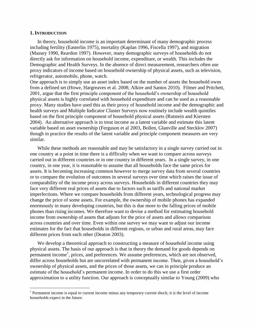
1. INTRODUCTION

In theory, household income is an important determinant of many demographic process

including fertility (Easterlin 1975), mortality (Kaplan 1996, Fiscella 1997), and migration

(Massey 1990, Reardon 1997). However, many demographic surveys of households do not

directly ask for information on household income, expenditure, or wealth. This includes the

Demographic and Health Surveys. In the absence of direct measurement, researchers often use

proxy indicators of income based on household ownership of physical assets, such as television,

refrigerator, automobile, phone, watch.

One approach is to simply use an asset index based on the number of assets the household owns

from a defined set (Howe, Hargreaves et al. 2008; Alkire and Santos 2010). Filmer and Pritchett,

2001, argue that the first principle component of the household’s ownership of household

physical assets is highly correlated with household expenditure and can be used as a reasonable

proxy. Many studies have used this as their proxy of household income and the demographic and

health surveys and Multiple Indicator Cluster Surveys now routinely include wealth quintiles

based on the first principle component of household physical assets (Rutstein and Kiersten

2004). An alternative approach is to treat income as a latent variable and estimate this latent

variable based on asset ownership (Ferguson et al 2003, Bollen, Glanville and Stecklov 2007)

though in practice the results of the latent variable and principle component measures are very

similar.

While these methods are reasonable and may be satisfactory in a single survey carried out in

one country at a point in time there is a difficulty when we want to compare across surveys

carried out in different countries or in one country in different years. In a single survey, in one

country, in one year, it is reasonable to assume that all households face the same prices for

assets. It is becoming increasing common however to merge survey data from several countries

or to compare the evolution of outcomes in several surveys over time which raises the issue of

comparability of the income proxy across surveys. Households in different countries they may

face very different real prices of assets due to factors such as tariffs and national market

imperfections. Where we compare households from different years, technological progress may

change the price of some assets. For example, the ownership of mobile phones has expanded

enormously in many developing countries, but this is due more to the falling prices of mobile

phones than rising incomes. We therefore want to devise a method for estimating household

income from ownership of assets that adjusts for the price of assets and allows comparison

across countries and over time. Even within one survey we may want to adjust our income

estimates for the fact that households in different regions, or urban and rural areas, may face

different prices from each other (Deaton 2003).

We develop a theoretical approach to constructing a measure of household income using

physical assets. The basis of our approach is that in theory the demand for goods depends on

permanent income1, prices, and preferences. We assume preferences, which are not observed,

differ across households but are uncorrelated with permanent income. Then, given a household’s

ownership of physical assets, and the prices of those assets, we can in principle produce an

estimate of the household’s permanent income. In order to do this we use a first order

approximation to a utility function. Our approach is conceptually similar to Young (2009) who

1 Permanent income is equal to current income minus any temporary current shock; it is the level of income

households expect in the future.

produces estimates of the growth rate of the standard of living in Sub-Saharan Africa that

combine estimates of health, education, consumption, and time use, where the consumption

component is proxied by asset ownership allowing for price changes over time. We show that in

a single survey, in which prices faced by all households are the same, we can estimate a measure

of household income as a common household random effect that affects the demand for each

good. The latent variable, or common factor approach, produces estimates that are highly

correlated with first principle component in practice. It follows that for a single survey in which

households all face the same prices for assets our approach is very similar to existing methods.

The advantage of using our approach become evident when we consider comparisons across

surveys that take place in different countries or in different years since we allow for differences

in the price of assets faced by different households. A second advantage of our latent variable

approach is that it allows for different surveys to have information on different sets of physical

assets (so long as there is at least one asset in common). All asset information present in each

survey can be used. In addition, if a household has missing data for an asset its income can still

be estimated from the data on asset ownership that we do have. Having information on a

restricted set of assets for some observations still allows us to estimate income for these

households though the precision of the estimate will be reduced.

The estimates of household income produced by our methods may be used in subsequent

regression analysis by researchers who wish to allow for the effect of household income on other

outcomes. Our estimates give the expected value of household income given the observed prices

and ownership of household physical assets. However our estimates contain parameter

uncertainty, and noise, and therefore should not be used in the same way as direct observation.

Using the income estimate directly will tend to lead to underestimation of the effect of income. A

simple parametric bootstrap can be used to generate a number of potential values of household

income drawn from the underlying distribution of income conditional on prices and asset

ownership. These multiple draws of potential values for household income can be used in

subsequent regression analysis in the same way as data generated for missing observations

through multiple imputation (Rubin 1987).

The paper is structured as follows. In section 2 we describe our theory-based estimation

approach and show how our method can be used to construct estimates of income that are

comparable over time and across countries. In section 3 we compare our income estimates for a

single survey with those from principle component analysis and with reported household income

and expenditure using surveys that contain both ownership of physical assets and data on income

and expenditure. In section 4 we estimate average national income for countries using survey

data on ownership of physical assets adjusting for country specific asset prices and compare our

estimates with the standard approach using national income accounts. We show how to generate

multiple estimates of income using our method that can be used in subsequent regression

analysis in section 5. In section 6, we discuss the limitations of our approach and possible future

developments. Section 7 concludes.

2. THEORY

Consider household i, in a survey k that takes place in county in a particular year. There are

n assets indexed by 1,....,j n whose ownership is determined by questions in at least one

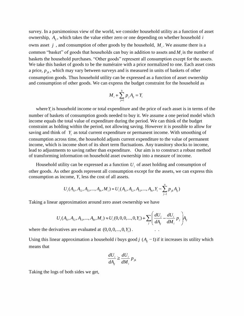
survey. In a parsimonious view of the world, we consider household utility as a function of asset

ownership, ijA , which takes the value either zero or one depending on whether household i

owns asset j , and consumption of other goods by the household, iM . We assume there is a

common “basket” of goods that households can buy in addition to assets andiM is the number of

baskets the household purchases. “Other goods” represent all consumption except for the assets.

We take this basket of goods to be the numéraire with a price normalized to one. Each asset costs

a price,jkp , which may vary between surveys and is measured in units of baskets of other

consumption goods. Thus household utility can be expressed as a function of asset ownership

and consumption of other goods. We can express the budget constraint for the household as

1

h

i j ij i

j

M p A Y

whereiY is household income or total expenditure and the price of each asset is in terms of the

number of baskets of consumption goods needed to buy it. We assume a one period model which

income equals the total value of expenditure during the period. We can think of the budget

constraint as holding within the period, not allowing saving. However it is possible to allow for

saving and think of iY as total current expenditure or permanent income. With smoothing of

consumption across time, the household adjusts current expenditure to the value of permanent

income, which is income short of its short term fluctuations. Any transitory shocks to income,

lead to adjustments to saving rather than expenditure. Our aim is to construct a robust method

of transforming information on household asset ownership into a measure of income.

Household utility can be expressed as a function iU of asset holding and consumption of

other goods. As other goods represent all consumption except for the assets, we can express this

consumption as income, Y, less the cost of all assets.

1 2 3 1 2 3

1

( , , ,..., , ) ( , , ,..., , )n

i i i i ih i i i i i ih i jk ij

j

U A A A A M U A A A A Y p A

Taking a linear approximation around zero asset ownership we have

1 2 3( , , ,..., , ) (0,0,0,...,0, ) i ii i i i ih i i i j ij

j ij i

dU dUU A A A A M U Y p A

dA dM

where the derivatives are evaluated at (0,0,0,...,0, )iY . . .

Using this linear approximation a household i buys good j ( 1)ijA if it increases its utility which

means that

i ijk

ij i

dU dUp

dA dM

Taking the logs of both sides we get,

log log logi ijk

ij i

dU dUp

dA dM

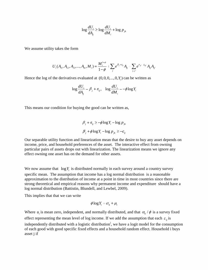
We assume utility takes the form

' '

1

1 2 3 '

, '

( , , ,..., , )1

j ij jj ijjii i i i in i ij ij ij

j j j

MU A A A A M e A e A A

Hence the log of the derivatives evaluated at (0,0,0,...,0, )iY can be written as

log , log logi ij ij i

ij i

dU dUY

dA dM

This means our condition for buying the good can be written as,

log logj ij i jkY p

log logj i jk ijY p

Our separable utility function and linearization mean that the desire to buy any asset depends on

income, price, and household preferences of the asset. The interactive effect from owning

particular pairs of assets drops out with linearization. The linearization means we ignore any

effect owning one asset has on the demand for other assets.

We now assume that log iY is distributed normally in each survey around a country survey

specific mean. The assumption that income has a log normal distribution is a reasonable

approximation to the distribution of income at a point in time in most countries since there are

strong theoretical and empirical reasons why permanent income and expenditure should have a

log normal distribution (Battistin, Blundell, and Lewbel, 2009).

This implies that that we can write

log i k iY

Where iu is mean zero, independent, and normally distributed, and that /k is a survey fixed

effect representing the mean level of log income. If we add the assumption that each ij is

independently distributed with a logistic distributioni, we have a logit model for the consumption

of each good with good specific fixed effects and a household random effect. Household i buys

asset j if

logk j jk i ijp

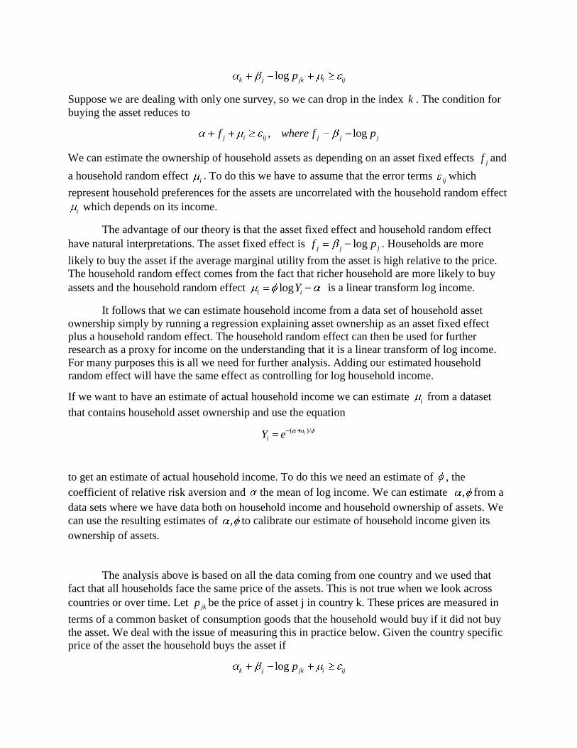
Suppose we are dealing with only one survey, so we can drop in the index k . The condition for

buying the asset reduces to

, logj i ij j j jf where f p

We can estimate the ownership of household assets as depending on an asset fixed effects jf and

a household random effect i. To do this we have to assume that the error terms

ijwhich

represent household preferences for the assets are uncorrelated with the household random effect

i which depends on its income.

The advantage of our theory is that the asset fixed effect and household random effect

have natural interpretations. The asset fixed effect is logj j jf p . Households are more

likely to buy the asset if the average marginal utility from the asset is high relative to the price.

The household random effect comes from the fact that richer household are more likely to buy

assets and the household random effect logi iY is a linear transform log income.

It follows that we can estimate household income from a data set of household asset

ownership simply by running a regression explaining asset ownership as an asset fixed effect

plus a household random effect. The household random effect can then be used for further

research as a proxy for income on the understanding that it is a linear transform of log income.

For many purposes this is all we need for further analysis. Adding our estimated household

random effect will have the same effect as controlling for log household income.

If we want to have an estimate of actual household income we can estimate i from a dataset

that contains household asset ownership and use the equation

( )/iu

iY e

to get an estimate of actual household income. To do this we need an estimate of , the

coefficient of relative risk aversion and the mean of log income. We can estimate , from a

data sets where we have data both on household income and household ownership of assets. We

can use the resulting estimates of , to calibrate our estimate of household income given its

ownership of assets.

The analysis above is based on all the data coming from one country and we used that

fact that all households face the same price of the assets. This is not true when we look across

countries or over time. Let jkp be the price of asset j in country k. These prices are measured in

terms of a common basket of consumption goods that the household would buy if it did not buy

the asset. We deal with the issue of measuring this in practice below. Given the country specific

price of the asset the household buys the asset if

logk j jk i ijp

Note that we keep jthe same across countries and time. This means the asset is on average

equally desirable in different countries and at different times. In one country we assumed that log

income was normally distributed around a country mean. When we have several countries we

assume that log income is normally distributed around a country mean in each country but the

country means can vary across countries. We can estimate this equation by regressing asset

ownership on a country fixed effect, an asset fixed effect, and a household random effect, and

allowing for the effect of asset prices jkp in each country, with a coefficient on the price effect

that is constrained to be minus one. We can then use the estimated values k i

as a proxy for

household income for household i in survey k. Note that in estimating this equation across

surveys the fixed effects on survey and assets are collinear. We therefore drop one of the survey

fixed effects, say 0on survey the baseline zero. This is not a problem if we wish only to have a

proxy for income since again we have that k i

is a linear transformation of log household

income. If we want to have an actual estimate for household income we need to calculate

0( )/k iu

iY e

We can do this by calibrating the link between the latent household variable and income from

the baseline survey to give estimates of 0 , and then use these estimates to give estimates of

household income across all our surveys. This means that if we want actual estimates of

household income we need to have a baseline survey in which we have both income and asset

data. Using this to calibrate 0 , we can then generate estimates of income in all the other

surveys using only their asset data.

Prices

To calculate the price of an asset in a survey we use data from the World Bank’s

International Comparison Program. This gives prices for categories of goods in local currency

units. It also estimates the cost in local currency units of a common basket of goods based on the

average consumption bundle bought worldwide. Let jkP be the price of the asset j in the country

at the time of the survey k measured local currency units. The International Comparison

Program takes pains to try to measure prices of the same or comparable goods across countries to

avoid quality differences. Let kP be the price in local currency units of the common basket of

goods as defined by the International Comparison Program in the same country at the same time.

Then we have that the real price of asset j in survey k is

/jk jk kp P P

For example, comparing Egypt and Colombia using the pjk for motorcycle and mobile phone:

pmotorcycle,Egypt = 4.52 is interpreted as 4.52 units of global basket of goods which can be purchased

with an amount equivalent to 1 motorcycle in Egypt. Similarly, pphone,Egypt =2.51 indicates about

2.51 units of global basket of goods can be purchased with the same amount it takes to purchase

a phone in Egypt. From this, we infer that a motorcycle in Egypt is more expensive than a phone.

When we compare Egypt to Colombia, we calculated pmotorcycle,Egypt=4.52 and

pmotorcycle,Colombia=3.72. We infer that an individual in Egypt who purchases a motorcycle would

forgo more units of global basket of goods compared to an individual in Colombia.

A common problem in this type of analysis is that the common basket of goods should be

representative of what people in each setting actually buy. If the goods consumed in the two

settings are very different the common basket may not be representative of either and resulting

estimates of income based on common basket of goods may be misleading (Deaton 1975).

Statistical Analysis

To estimate permanent incomes, we employ a multilevel logit model of the following form:

logit(Pr( 1)) logijk k j jk iA p

)1(

where ijkA is a binary indicator for holding an asset j in household i within survey k. Note that

the number of observations in this regression is the number of surveys, times the numbers of

households, times the number of assets. That is, we have a separate observation for each asset. If

we are estimating with only one survey and can assume priced faced by each household are the

same this reduces to

logit(Pr( 1))ij j iA

Where j is an asset fixed effect and i is household income. We calibrate the model in four

different economic contexts: Tanzania 2004, Peru 1994, South Africa 1994 and Egypt 1988,

2005 using data from Living Standard Measurement Surveys (LSMS) in each country that

include information on household income and expenditure, and household assets. We treat each

survey independently and compare our estimates of household income based on assets with the

reported information on income and expenditure.

All available household assets except bicycle in the individual LSMS surveys were used in

the generation of household wealth estimate. Our model implies that ownership of each asset

should increase on average with income. Preliminary studies showed that ownership of all other

assets increased with income and expenditure. However, bicycle ownership first rises with

income and then falls. It may be that car and bicycle ownership are strong substitutes. When

households own a car the benefits of a bicycle become very small. This will appear in the

interactive term between asset owned in our utility function but is ignored by our linearization.

To properly model bicycle ownership we would require at least a second order approximation to

the utility function that allowed for these interactive effects. We therefore propose that assets

such as bicycles whose ownership does not increase with income be dropped from the analysis

when our linear approximation to the utility function is used.

The estimates are compared with reported household income and expenditure. South Africa

1994 was further used in regressions between household expenditure and the estimated wealth

index, along with other socio-demographic covariates such as cluster-level electricity access,

urban rural location, household highest education level, household size, percentage of children

(<15 years old) and percentage of adult females. DHS Egypt survey 1988 and 2005 were used to

demonstrate temporal comparison within a country. Seven asset types were used to generate the

household wealth estimate. Mean wealth index percentiles were compared across the survey

years to explore trends in household wealth. Cross-country comparison of absolute wealth index

uses households from 225 DHS and MICS surveys of 117 low- and middle-income countries

completed as early as 1990 and as late as 2008.

Data Sources

Household level Data

The household level data sources for the empirical analysis are from the Demographic and

Health Surveys (DHS), Multiple Indicator Cluster Surveys (MICS), and the Living Standards

Measurement Study Surveys (LSMS). Each of these surveys contains data on fertility behavior

and household health and socio-economic status. Table 1 shows the distribution of the surveys

over time and across regions. Our sample consists of households from 225 surveys of 117 low-

and middle-income countries completed as early as 1990 and as late as 2008.

The DHS is a nationally representative, cluster randomized household survey initiated in the

late 1980s by the US Agency for International Development. The DHS contains household

characteristics. And gives a particular focus on women aged 15-49 and children, but also

information on men aged 15-54 or 59 in more recent surveys. The surveys have a common

design, with some variation in specific questions across countries and a wider range of variables

available in recent waves. The survey is an ongoing initiative, and has come to span 73

developing countries with up to five survey waves in each country. There are 181 standardized

(recoded) and publicly available country surveys. We have merged these surveys into a single

dataset for statistical analysis.

The Multiple Indicator Cluster Surveys (MICS), published by UNICEF, is a household

survey carried out in a range of countries in 1998 designed to complement the DHS. The MICS

focus on childhood health, and nutritional status, with additional data on standards of living

based on household ownership of assets and housing construction. In our study, we used MICS

Wave 3, which includes 44 surveys from 44 countries.

The Living Standards Measurement Study (LSMS) has the advantage of having detailed

information on household income and expenditure, as well as individual earnings. It is used in

our study to help elucidate the relationships between our wealth estimate and self-reported,

cross-sectional income and expenditure. From 1985 to present, there are 32 participating

countries, with multiple survey waves in 17 countries and panel datasets for 9 countries. We will

use these data to validate and demonstrate application of our household income estimates.

Country level Data

Country level data include country-specific prices of assets from the World Bank’s

International Comparison Program (ICP) and international indices from the Multi-Dimensional

Poverty Index (MPI) and Human Development Indicator (HDI), as well as real GDP per capita

estimates from the Penn World Tables (PWT).

The ICP provided country-specific, internationally comparable price levels and purchasing

power parities (PPPs) from 2005. The PPPs are derived from global program of national surveys

that priced nearly 1000 products and services from 146 economies. The country-specific PPPs

and expenditures are further divided into 129 basic headings of similar goods or services such as

“major household appliances”, “small electric household appliances”, “motor cars”, “telephone

and telefax equipment”, “jewelry, clocks and watches”.

The Penn World Table (PWT) displays a set of national accounts economic time series

covering many countries. Its expenditure entries are denominated in a common set of prices in a

common currency so that real quantity comparisons can be made, both between countries and

over time. It also provides information about relative prices within and between countries, as

well as demographic data and capital stock estimates. PWT uses ICP benchmark comparisons as

a basis for estimating PPPs for non-benchmark countries and extrapolates backward and forward

in time. The PWT 6.3 covers 190 countries and territories, 1950-2009, 2005 as reference year.

The Human Development Index (HDI), published by United Nations Development

Programme (UNDP), provides a composite score based on three dimensions: 1. Life expectancy,

2. Education: mean years of schooling for adults and expected years of schooling of children 3.

Living standards: gross national income per capita. The HDI uses the logarithm of income, to

reflect the diminishing importance of income with increasing gross national income. The scores

for the three HDI dimension indices are then aggregated into a composite index using geometric

mean. The index covers 195 countries over 30 years.

Life expectancy at birth is provided by the UN Department of Economic and Social Affairs;

mean years of schooling by Barro and Lee (2010); expected years of schooling by the UNESCO

Institute for Statistics; and GNI per capita by the World Bank and the International Monetary

Fund. For few countries, mean years of schooling are estimated from nationally representative

household surveys such as the WFS and DHS.

The Multidimensional Poverty Index (MPI) is a new international measure of poverty

developed by the Oxford Poverty and Human Development Initiative (OPHI) and the UNDP

Human Development Report in 2010. It covers 104 developing countries. The MPI uses 10

dichotomized depravation indicators: nutrition, child mortality, year of schooling, school

enrollment, and standard of living: cooking fuel, sanitation, drinking water, electricity, floor and

asset ownership. The data is based on three sources: DHS, MICS and the World Health Survey.

MPI is reported to be robust, where 95% of country comparisons do not change if the poverty

cutoff ranges from 20% to 40% of the dimensions. MPI is also robust to weight variations. (MPI,

2010)

3. HOUSEHOLD INCOME WITHIN COUNTRY: COMPARISON WITH PRINCIPLE COMPONENT

ANALYSIS

The approach used in this study offers an avenue to determine household level income from a

list of asset holdings. The household level and the macro-cross country results allow us to

discuss this methodological approach compared to existing methods and interpret the results with

theoretical basis.

Household Level Validation of Income Estimates

While the aim is to estimate a measure of household income that is comparable across

countries, we will check our functional form for the utility of other goods and estimate

correlation and the coefficient of relative risk aversion, , using data from surveys that contain

both income and asset holdings. Examples of this are the three LSMS three countries selected for

household level validation: Peru, Tanzania and South Africa.

Looking at the correlation between the generated income estimates and self-reported

household annual income and expenditure in the three surveys, we find that the correlation with

income are consistently lower than with expenditure. Many households reported zero income in

the past 12 months from the LSMS surveys. This dramatically reduce the sample size when we

take the natural log of income in our model, i.e.in Tanzania LSMS 1994, sample size reduced by

over 50% (Table 4).

Our correlation of wealth estimate and household annual expenditure are 0.75, 0.70, 0.68,

and with household annual income are 0.70, 0.40, 0.59 for South Africa, Tanzania and Peru,

respectively. Compared to method of principal component analysis (PCA), the correlations with

expenditure are similar in all three countries (Table 4). An important aspect of our income

estimation model is the resulting constant coefficient of relative risk aversion. This coefficient

enables extrapolation of household level income and expenditure from historical surveys that had

data on asset holding but may not contain income or expenditure data. The coefficient, ρ, linearly

transforms log of reported income or expenditure to income estimate. The coefficient is based on

the Arrow-Pratt measure of relative risk-aversion where the utility function changes from risk-

averse to risk-loving as income changes. For income, the coefficient lies below 1.0; for

expenditure, the coefficient lies close to 1.0 for all households (Table 5).

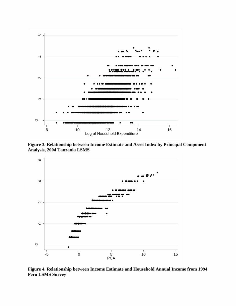
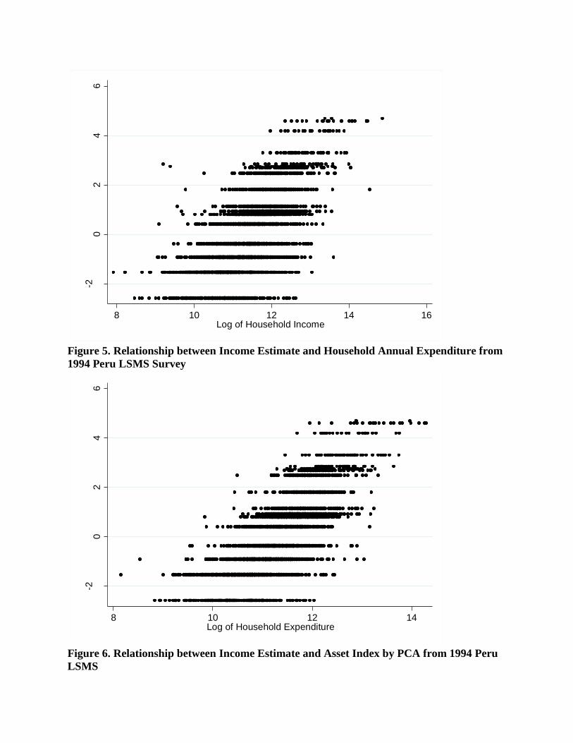
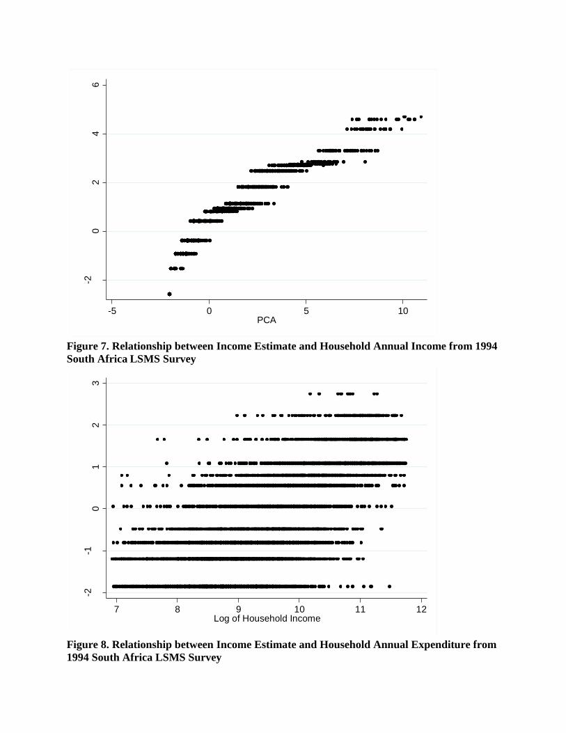
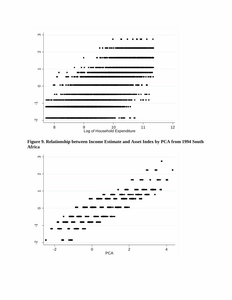
Figure 1 to 9 depict graphically the relationship between income estimate and reported

income, expenditure and asset index from PCA in three countries. Each household represent a

data point in the graph. The lower the income estimate, the poorer the households were

according to the index generated by this approach. In South Africa, income estimate is linearly

associated with household reported income and expenditure. Each income estimate value from

the developed index corresponds to a range spanning approximately 104 South African Rand

(ZAR) of composite household income and household expenditure. The range begins to widen as

households are positioned poorer on the estimation. This trend is more pronounced in Peru,

where the range of household reported income and expenditure corresponding to income

estimate gradually increase toward the poorer end of the spectrum. In 1994 Peru LSMS, the

maximum range in the lowest end of the income estimate span 105

Peruvian Nuevo Sol (PEN) in

household reported income and expenditure. In Tanzania, the estimate exhibited a less defined

linear association with household reported income and expenditure. The graphs exhibit bottom

heavy association similar to South Africa and Peru. Furthermore, the income estimate is discrete

in the index due to finite combination of asset holdings in the households, whereas reported

income and expenditure are continuous variables.

Income Estimates across Time: DHS Egypt 1988 and 2005

Egypt from DHS was selected as it satisfied the criteria of having multiple survey years in

the standard DHS and survey years close to available benchmark price data from Penn World

Table. Comparable benchmark data from 1985 and 2005 were used to adjust for asset-specific

prices in generation of the income estimate. There were 9,803 households surveyed in Egypt

1988 and 21,965 in 2005. The mean income estimate for households surveyed in 1988 were

similar to ones in 2005 in the richest and middle tertiles. In the poorest tertile, the mean income

estimate increased from -1.21 (SD 0.60) to -1.07 (SD 0.72) from 1988 to 2005. Figure 10

indicates a decrease in percent of households at -1 on the income estimate and increase in percent

of households with middle income estimates. We note that the absolute minimum income

estimate for households is lower in 2005 than in 1988 even though more percentage of

households scored below 0 on the income estimate in 1988.

4. HOUSEHOLD INCOME ACROSS COUNTRIES: COMPARISONS WITH INTERNATIONAL INDICES

There were 2,291,362 total households across 117 countries from 1985 – 2008 included from

181 DHS and 44 MICS Wave 3. The seven assets holdings considered include television,

refrigerator, motorcycle or scooter, car or truck, mobile phone, non-mobile phone, and watch.

Table 7 shows the percentage of households reporting asset holdings averaged across countries

by survey year. 47.0% of all households reported owning a TV, 34.1% owning a refrigerator,

8.9% own a motorcycle, 13.2% a car or truck, 22.5% a mobile phone, 19.3% a non-mobile phone

and 10.7% a watch. There were considerable missing data from households for two assets:

57.8% of households had missing data on non-mobile phone and 83.9% on watch.

Stratified by survey year, we note that higher percent of households surveyed from 2001-2005

reported owning assets compared to households surveyed before 2001. We estimated the

household income estimate which has a distribution around the mean of 0.0243 with a standard

deviation of 0.6313, a minimum of -1.9139 and maximum of 3.4954.

We selected the most recent surveys from 84 countries in the DHS and MICS3 and correlated

their average household income estimate with Real Gross Domestic Income, the international

dollar (I$) terms of trade adjusted GDP (Figure 11). The correlation is 0.64. We observe that

countries with relatively higher GDP generally have a higher mean income measure and

countries with relatively lower GDP have a lower mean income measure. The correlation is not

high, that is, countries that reported similar GDP levels could have a mean income measure that

differs by 2 to 3 units cross our income estimate.

The independent variable is taken from the constant price Real Gross Domestic Income

adjusted for Terms of trade changes in the Penn World Table 6.3

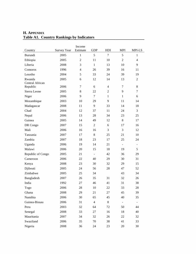
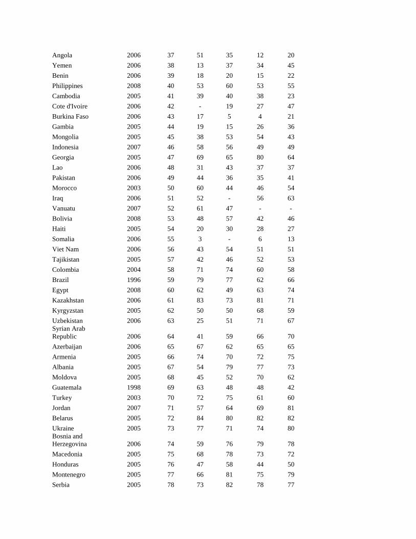
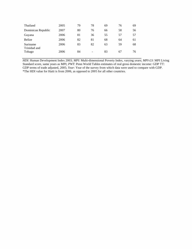
Table A1 displays the country rankings for income estimate and four other indicators: the

HDI, MPI, MPI Living Standard score (MPI-LS), and PWT. In the ranking a 1 indicates poorest

by the particular measure, and higher numbers indicate higher degree of income by the measure.

In our initial results, we find a high, though not perfect, degree of similarity between our global

ranking and country ranks from other metrics. The correlations between the values of income

index and the values of GDP per household, HDI, MPI, MPI-LS, are 0.63, 0.65, 0.74, 0.83, 0.84

and 0.89, respectively. The lowest correlation is found with the measure of country GDP

adjusted for household consumption, while the highest is found with the MPI-LS, which was

derived from similar data.

5. HOUSEHOLD INCOME USED IN SUBSEQUENT REGRESSION ANALYSES

We performed sensitivity analysis by stratifying cluster-level electricity access in order to

explore bias in using durable electrical goods as asset types. Clusters with high level of access to

electricity are defined by more than 5% households reporting use of electricity for lighting. In

correlating our income estimate and income or expenditure, households that are in clusters with

high level of access to electricity are similar to all households together, but clusters with low

level of electricity access had much lower correlation coefficients.

Reported income and expenditure exhibit different correlation patterns with the income

estimate when stratified by electricity access. Compared with the correlation between income

estimate and reported income in all households, correlation based on households in clusters with

high level of electricity access was slightly increased. The increased correlation is

understandable since our income estimate is generated by ownership of durable electrical goods

such as TV and refrigerator. Conversely, households in clusters with low access to electricity

have much lower correlation between reported income and income estimate. This correlation

pattern of income estimate with reported income was found both in Tanzania and South Africa.

All clusters in Peru had over 50% of households reporting access to electricity. Hence

households in Peru were not stratified by cluster-level electricity access (Table 4).

The pattern was not apparent when correlating with expenditure. In Tanzania, all households

and households in cluster with high electricity access and low electricity access had very similar

level of correlation (r = 0.69). In South Africa, correlation in households in cluster with low

electricity access have lower correlation (r = 0.43) than households in clusters with high

electricity access (r = 0.76) and all households (r = 0.78).

Similar patterns from cluster-level electricity stratification were found in coefficient of

relative risk aversion. The coefficients generated from households in clusters with high

electricity access are greater than coefficient generated from households in clusters with low

electricity access for household income and expenditure (Table 9)

Our income estimate significantly associates with the log of household expenditure (p= <

0.001, R2 = 0.566). When we incorporate additional socio-demographic variables such as

electricity, education level and household composition, the association improved 11% (R2 =

0.631). The R2 ratio exceeds 0.89 and a joint F-test on all independent variables except income

estimate rejected the null hypothesis that none of the socio-demographic variables together have

predictive power (F = 199.07, p< 0.001).

6. DISCUSSION

There are five major findings from this study. First, the income estimate generated from

household asset holdings correlates closely with household expenditure within each country

study and is comparable to the correlations between asset index generated from PCA and

expenditure. Secondly, we generate from the income estimate in LSMS the corresponding

coefficient of relative risk aversion. From this coefficient, we are able to extrapolate household

income and expenditure based on short list of asset holding data. The method allow for

interpretation of the household random effect as the marginal utility of money. Thirdly, we

demonstrated a shift in household income within a country through comparison across time.

Moreover, cross-country comparison with established indices such as the trade and consumption

adjusted GDP illustrated a high correlation at the country-aggregate level. We found that our

index rank similarly with other indices such as the Multi-dimensional Poverty Index and the

Human Development Index. Lastly, we incorporated socio-demographic factors along with our

income estimate to explore a more complex model associated with household income and

expenditure. We found that the income estimate accounts for over 89% of variance in household

expenditure and the additional socio-demographic factors increase the association by

approximately 11%. From our methods and results, we will discuss similarities and differences

found across the country studies, corroboration and contradictions with other wealth indicators,

the strengths and limitations of our approach and the usability and application for other

researchers.

Income Estimate at the Household Level

Generating the income estimate in Peru, Tanzania and South Africa illustrated some

overarching characteristics. Overall, Peru and Tanzania had a lower correlation with household

income than South Africa. Correlation with expenditure across the three countries are above 0.6,

where South Africa has the highest correlation of the three. There is variation across countries in

the performance of the income estimate. Correlation with expenditure is consistently higher than

with income in the three countries. The household annual income and expenditure from each

country survey were constructed differently from various components of income and expenditure

sources. There is evidence that income, expenditure measure constructed from component

sources allow respondents to provide a more accurate amount earned and spent in the past 12

months including sources that may not be traditionally considered as income, such as remittance

or crop sales and expenditure such as seasonal religious offerings. (Smeeding and Weinberg,

2001)

Stratification based on cluster access to electricity captures wealth gradient within the same

neighborhood while adjusting for bias to ownership of electrical durable goods. The small

percentage of households that reported having access to electricity may own a private generator.

When stratified by high or low electricity access, correlation of the asset-based wealth index and

household income and expenditure dramatically decreased in clusters with low access to

electricity. This difference in correlation suggests that the wealth index is a much stronger proxy

for household wealth in areas where household access to electricity and is a weaker proxy in

remote areas where access to electricity is very low. Although this difference exist, other

commonly used methods in determining household wealth, such as the principal components

analysis, is predominantly used regardless of electricity access.

Comparison with Principal Components Analysis

Filmer and Pritchett (2001) incorporated asset ownership and household characteristics in

creating an asset index as a proxy of long-term household welfare. They used statistically

procedure of principal components to determine the weights for an index of the asset variables.

They tested reliability of the PCA method in the context of India states. The results showed

internal coherence, robustness in assets included and comparability to state-level poverty status.

One of the drawbacks that they noted was also between urban and rural comparisons. When used

only eight asset ownership variables, they had a 0.79 correlation coefficient in the classification

of the poorest 40%, compared to when using their full model, where they included eight asset

ownership, drinking water source, toilet type, housing characteristics and land acre ownership.

Our income estimates from LSMS South Africa, Peru and Tanzania correlate highly with the

asset index using the PCA method (Table 4) Principal Components Analysis is predominately

used when investigating questions within a region or a country, where the list of assets is fixed

for all surveys. When comparing across survey years and across multiple countries or regions,

the proposed income estimation provides an additional avenue to approach such research

questions.

Income Estimate Across Survey Years

Generating a proxy for wealth across time was demonstrated in DHS Egypt survey year 1988

and 2005. We aimed to use price data to adjust for asset ownership preferences. According to the

wealth index, we found that the poorest tertile has an increase in household wealth from 1988 to

2005, whereas, no significant changes were found in the middle and rich tertile. Similar pattern

across time was found when we did not control for prices of assets. When price data is

unavailable, the results suggest that the proposed wealth estimate maintains its robustness.

Income Estimate Across Countries

Results of wealth index generated across countries using data from DHS and MICS were

comparable to international indices such as the Penn World Table, Multidimensional Poverty

Index and Human Development Index. Since MPI uses WFS, DHS data sources similar to ones

used in the current study, it is expected that the MPI Living Standard score correlates very

closely with our index. The correlation with log of trade adjusted GDP suggests that in general,

the mean income estimate of each country is comparable with national GDP. At the same time,

there are countries with similar ranking on the estimate but ranges by 104 in the real gross

domestic income. Conversely, we see countries reported similar GDP levels would be ranked

within a large range across the estimate. This correlation pattern indicates that at the mean

country level, the income estimate should be interpreted descriptively with caution as a proxy for

countries welfare or poverty level.

Incorporation of Socio-Demographic Factors

At the household level, our income estimate performs well, accounting for 58% of the

variance of the log of household expenditure in LSMS South Africa 1994. Adding socio-

demographic variables improved the regression fit by 11%. This amounts to an R2 ratio of 0.89,

suggesting that the estimates generated from the asset holdings provide a reliable proxy for

household expenditure and long-term welfare.

Strengths and Limitations

Our income estimation has a number of strengths as well as limitations. Firstly, the

estimation is methodologically based on economic consumption theory. It uses a household

utility function with a simple form of marginal utility for each person. The theoretical basis

enables clear interpretation of the random effects as the marginal utility of money generated from

our analysis. This allows researchers to probe deeper regarding wealth and wealth in relation to

household consumption patterns. The theoretical framework also enables us to find the

coefficient of relative risk aversion. This coefficient leads us to our second advantage of the

income estimation. The coefficient developed from LSMS or other survey data which contains

both asset holding and income or expenditure measures can be used in another comparable

population to extrapolate income or expenditure values from household asset data only. This

provides a way to build reliable income measures from current data that lack detailed

expenditure or income measures; to create panel or longitudinal datasets with historical data.

Across countries, we demonstrated using our income estimate as an absolute wealth

index by using a common set of household durable goods and adjusting price of assets across

countries. The short list of asset types produced robust definition of wealth at the household level

across countries. Furthermore, the method used in generating the household wealth allows

missing data of asset holdings to exist. Households that had data, regardless of owning the asset

or not, in at least one asset type would have a random effects wealth estimate generated from it.

This is advantageous over PCA since the household is not excluded due to missing data unless

all asset holding data are missing.

A household income estimate at the micro-level and comparable across countries will expand

the type of international comparison studies which can be applied to poverty surveillance in a

neighboring regions, comparing the link between economic wellbeing and healthy aging.

Moreover, the income estimate in relation to household consumption improves rigorous studies

on household consumption, for example, income shocks from retirement pension plans and

consumption smoothing as aging adult transition out of the labor market.

While applying this theoretically-based method, we are cognizant of its assumptions and

limitations. We performed sensitivity analysis for two countries: Tanzania and South Africa. We

used composite measure of income and expenditure to correlate with our income estimate.

Although composite measure of income is a more reliable measure than a single self-reported

amount of household income, many households reported zero income in the past 12 months in

the LSMS surveys. This dramatically reduces the sample size when we take the natural log of

income in our model. In Tanzania LSMS 1994, sample size reduced by over 50%. Other studies

have noted that expenditure is a more reliable measure of standard of living and wealth across

life span (Morris, Carletto et al, 2000). It also leads to questions concerning debt, or negative

income, subsistence production of food and measurement error. This data limitation leads us to

rely more on the expenditure measure provided.

We stratified clusters into high and low access to electricity defined by at least 5% household

reported using electricity as an energy source for lighting. We found that our index correlates

with income much better in cluster with high electricity access than low electricity access. In

clusters with low electricity access, there is a 40 – 50% decrease in correlation, to 0.25 – 0.32.

This pattern was also present in correlation with expenditure in South Africa. We wanted to test

if the list of household durables would bias the income ranking of household with electricity

access as a confounder. Since many of the asset types used in generating the income estimates

require electrical energy source (besides battery or gasoline powered items), one major limitation

is that the index does not adequately capture income in areas with low electricity access. We

considered land, livestock and non-electrical agricultural tools as potential asset types. These

were not used because our theoretical framework applies to consumption items rather than

production items typical of land, livestock and tools. Although we aim to select household

consumer goods for consumption rather than production, there are items which are ambiguously

categorized. Automobiles may be transportation mean to work place. Mobile phones have been

shown as a crucial technological asset to allow farmers and producers of other goods to find a

market that have better commodity offers and bids (Mukhebi, 2007) Moreover it is difficult to

define goods such as bicycle as a normal good. Bicycle can be a mode of transportation when a

household cannot afford motorcycle or cars, but can also be owned by wealthy households for

leisure activities. The Indian Human Development Survey adopts a consumption per capita score

where ownership of a typically more expensive good (e.g. motor cycle or car) would recode the

household as owning a less expensive good (e.g. bicycle) as well. They found that without the

modification, less expensive items did not scale well; a household might not own some items

because they are too affluent or too poor. Our approach is not a summation scale of asset

ownership, but the index is generated through price adjusted, constant preference utility function.

One minor limitation would be these asset types must exist technologically before surveys can

collect data on household ownership of these assets. One example in Peru 1994 LSMS used

microwave as one of its household assets. When linking with historical data, common asset items

should be used.

Across countries, we used a short list of seven asset types that are majority cultural invariant

such as TV, refrigerator, motorcycle, mobile phones, etc. Considerable missing data from

households for “non-mobile phone” and “watch” is a limitation. Earlier survey waves may have

less comprehensive list of assets than later years and training of surveyors may have improved in

subsequent waves of data collection. The prices for each asset are based on PPP from ICP report

in 2005. Not all seven assets have its own distinct product categories, as we had access to only

basic heading prices such as “major household appliances (electric or not)”, “telephone and

telefax equipment” and ‘jewelry, clocks and watches”, “motor cars”, “motor cycle”. Finer details

in price data would improve income differentiation among households. Furthermore, as seen

from the sensitivity analysis, the residual, ε, is not independent and identically distributed.

Countries with large regional differences in culture and consumption patterns are also assumed

to have similar preferences in asset ownership with αk as a country fixed effect. These

assumptions are necessary to simplify household consumption behavior in our model, while

capturing the diverse income and expenditure levels across countries and across time. Generating

an absolute income estimate from all households in all countries and survey waves within the

DHS and MICS is computationally intensive. Moreover, each time a new country survey is

added to the panel dataset, the corresponding income estimate for the original set of households

would change, incorporating the newly added data.

7. USABILITY AND FUTURE DIRECTIONS

We applied our theoretically-based approach in three different sources of micro-level data:

DHS, MICS, LSMS. The model included price and country fixed effects when comparing across

countries but excluded them when analyzing within country. We aim to bolster our

understanding of this method by repeating the correlation analysis in other LSMS country

surveys as well as datasets that contain detailed asset holding, composite income and expenditure

data. Furthermore, correlation with household education attainment used similarly by Young

(2005) as a proxy for income in DHS would test the robustness of this index as a standard of

living measure. Beyond validating this novel approach, we aim to device a new global poverty

count used on the measure of wealth. We aim to compare this poverty count with other

international indices such as the MPI which includes asset holdings, education, housing quality

as well as other measures to denote deprecation in standard of living. Furthermore, the

internationally comparable income estimate can be used to measure inequality comparable to the

Gini coefficient at the regional, national and global level. A reliable measure of income at the

household level would provide valuable information of only poverty distribution and patterns,

but also on inequality of economic wellbeing, keeping in mind that it is only a part of the goal of

improving quality of life in societies.

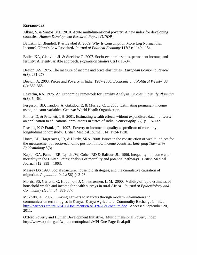
REFERENCES

Alkire, S, & Santos, ME. 2010. Acute multidimensional poverty: A new index for developing

countries. Human Development Research Papers (UNDP).

Battistin, E, Blundell, R & Lewbel A. 2009. Why Is Consumption More Log Normal than

Income? Gibrat's Law Revisited. Journal of Political Economy 117(6): 1140-1154.

Bollen KA, Glanville JL & Stecklov G. 2007. Socio-economic status, permanent income, and

fertility: A latent-variable approach. Population Studies 61(1): 15-34.

Deaton, AS. 1975. The measure of income and price elasticities. European Economic Review

6(3): 261-273.

Deaton, A. 2003. Prices and Poverty in India, 1987-2000. Economic and Political Weekly 38

(4): 362-368.

Easterlin, RA. 1975. An Economic Framework for Fertility Analysis. Studies in Family Planning

6(3): 54-63.

Ferguson, BD, Tandon, A, Gakidou, E, & Murray, CJL. 2003. Estimating permanent income

using indicator variables. Geneva: World Heatlh Organization.

Filmer, D, & Pritchett, LH. 2001. Estimating wealth effects without expenditure data – or tears:

an application to educational enrollments in states of India. Demography 38(1): 115-132.

Fiscella, K & Franks, P. 1997. Poverty or income inequality as predictor of mortality:

longitudinal cohort study. British Medical Journal 314: 1724-1728.

Howe, LD, Hargreaves, JR, & Huttly, SRA. 2008. Issues in the construction of wealth indices for

the measurement of socio-economic position in low income countries. Emerging Themes in

Epidemiology 5(3).

Kaplan GA, Pamuk, ER, Lynch JW, Cohen RD & Balfour, JL. 1996. Inequality in income and

mortality in the United States: analysis of mortality and potential pathways. British Medical

Journal 312: 999 – 1003.

Massey DS 1990. Social structure, household strategies, and the cumulative causation of

migration. Population Index 56(1): 3-26.

Morris, SS, Carletto, C, Hoddinott, J, Christiaensen, LJM. 2000. Validity of rapid estimates of

household wealth and income for health surveys in rural Africa. Journal of Epidemiology and

Community Health 54: 381-387.

Mukhebi, A. 2007. Linking Farmers to Markets through modern information and

communication technologies in Kenya. Kenya Agricultural Commodity Exchange Limited.

http://partners.cta.int/KACE/Documents/KACE%20eBrochure.doc. Accessed September 20,

2011.

Oxford Poverty and Human Development Initiative. Multidimensional Poverty Index

http://www.ophi.org.uk/wp-content/uploads/MPI-One-Page-final.pdf

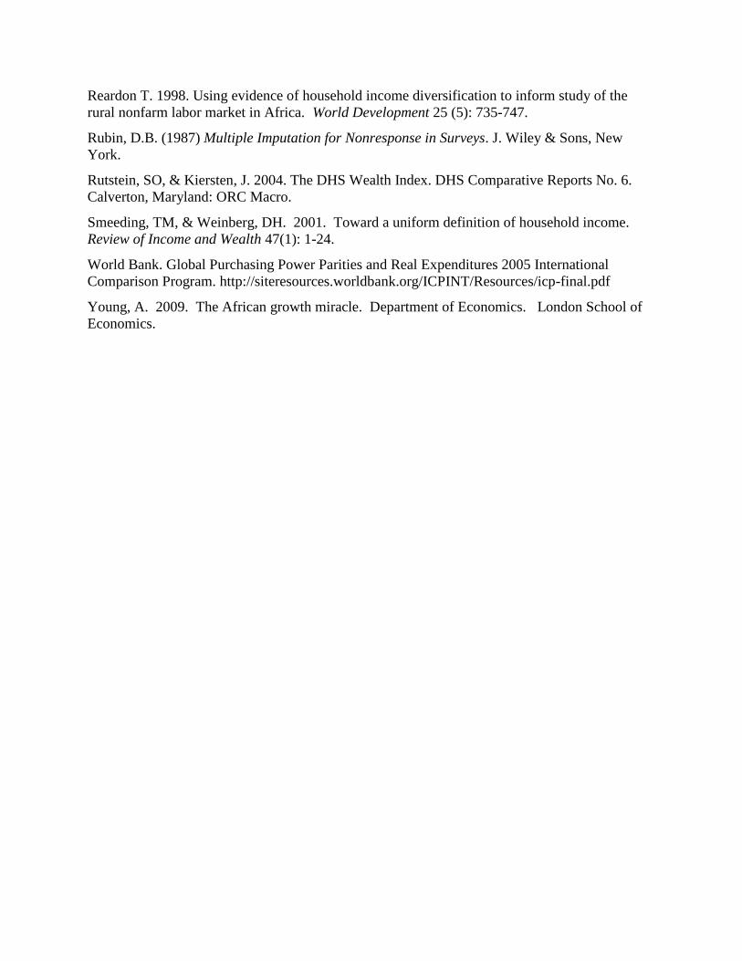
Reardon T. 1998. Using evidence of household income diversification to inform study of the

rural nonfarm labor market in Africa. World Development 25 (5): 735-747.

Rubin, D.B. (1987) Multiple Imputation for Nonresponse in Surveys. J. Wiley & Sons, New

York.

Rutstein, SO, & Kiersten, J. 2004. The DHS Wealth Index. DHS Comparative Reports No. 6.

Calverton, Maryland: ORC Macro.

Smeeding, TM, & Weinberg, DH. 2001. Toward a uniform definition of household income.

Review of Income and Wealth 47(1): 1-24.

World Bank. Global Purchasing Power Parities and Real Expenditures 2005 International

Comparison Program. http://siteresources.worldbank.org/ICPINT/Resources/icp-final.pdf

Young, A. 2009. The African growth miracle. Department of Economics. London School of

Economics.

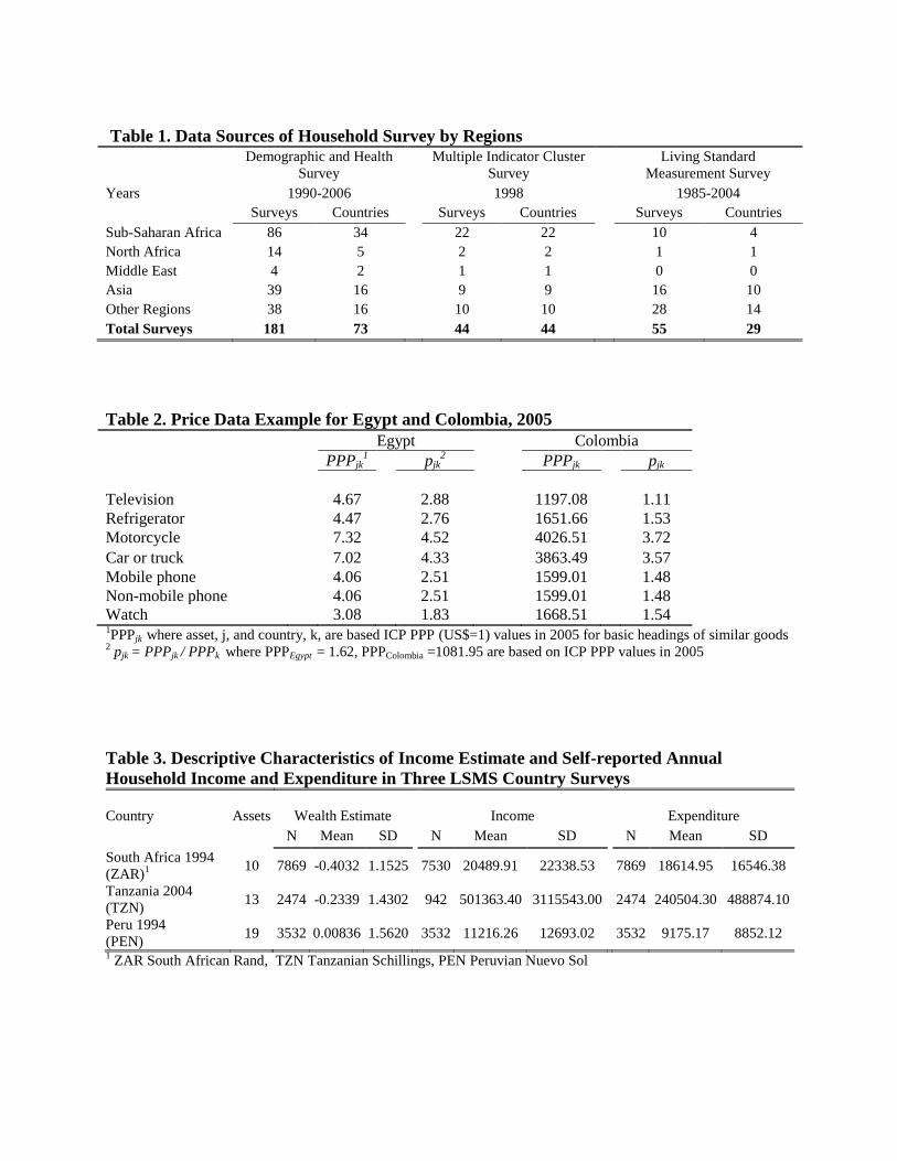
Table 1. Data Sources of Household Survey by Regions Demographic and Health

Survey

Multiple Indicator Cluster

Survey

Living Standard

Measurement Survey

Years 1990-2006 1998 1985-2004

Surveys Countries Surveys Countries Surveys Countries

Sub-Saharan Africa 86 34 22 22 10 4

North Africa 14 5 2 2 1 1

Middle East 4 2 1 1 0 0

Asia 39 16 9 9 16 10

Other Regions 38 16 10 10 28 14

Total Surveys 181 73 44 44 55 29

Table 2. Price Data Example for Egypt and Colombia, 2005

Egypt Colombia

PPPjk1

pjk2

PPPjk

pjk

Television

4.67 2.88 1197.08 1.11

Refrigerator

4.47 2.76 1651.66 1.53

Motorcycle 7.32 4.52 4026.51 3.72

Car or truck 7.02 4.33 3863.49 3.57

Mobile phone 4.06 2.51 1599.01 1.48

Non-mobile phone 4.06 2.51 1599.01 1.48

Watch 3.08 1.83 1668.51 1.54 1PPPjk where asset, j, and country, k, are based ICP PPP (US$=1) values in 2005 for basic headings of similar goods

2 pjk = PPPjk / PPPk where PPPEgypt = 1.62, PPPColombia =1081.95 are based on ICP PPP values in 2005

Table 3. Descriptive Characteristics of Income Estimate and Self-reported Annual

Household Income and Expenditure in Three LSMS Country Surveys

Country Assets Wealth Estimate

Income

Expenditure

N Mean SD N Mean SD N Mean SD

South Africa 1994

(ZAR)1

10 7869 -0.4032 1.1525 7530 20489.91 22338.53 7869 18614.95 16546.38

Tanzania 2004

(TZN) 13 2474 -0.2339 1.4302 942 501363.40 3115543.00 2474 240504.30 488874.10

Peru 1994

(PEN) 19 3532 0.00836 1.5620 3532 11216.26 12693.02 3532 9175.17 8852.12

1 ZAR South African Rand, TZN Tanzanian Schillings, PEN Peruvian Nuevo Sol

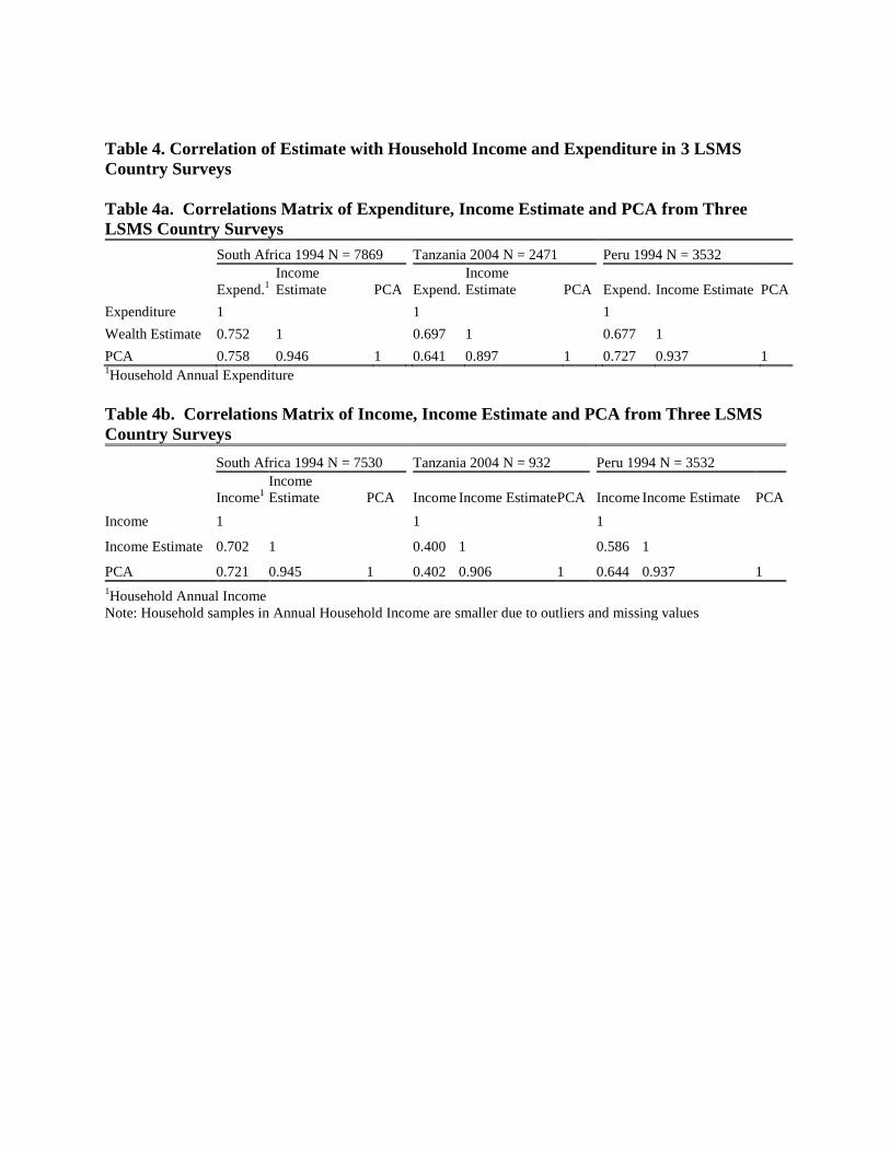
Table 4. Correlation of Estimate with Household Income and Expenditure in 3 LSMS

Country Surveys

Table 4a. Correlations Matrix of Expenditure, Income Estimate and PCA from Three

LSMS Country Surveys

South Africa 1994 N = 7869 Tanzania 2004 N = 2471 Peru 1994 N = 3532

Expend.1

Income

Estimate PCA

Expend.

Income

Estimate PCA

Expend. Income Estimate PCA

Expenditure 1 1 1

Wealth Estimate 0.752 1 0.697 1 0.677 1

PCA 0.758 0.946 1 0.641 0.897 1 0.727 0.937 1 1Household Annual Expenditure

Table 4b. Correlations Matrix of Income, Income Estimate and PCA from Three LSMS

Country Surveys

South Africa 1994 N = 7530 Tanzania 2004 N = 932

Peru 1994 N = 3532

Income1

Income

Estimate PCA

Income Income Estimate PCA

Income Income Estimate PCA

Income 1 1

1

Income Estimate 0.702 1 0.400 1

0.586 1

PCA 0.721 0.945 1 0.402 0.906 1

0.644 0.937 1

1Household Annual Income

Note: Household samples in Annual Household Income are smaller due to outliers and missing values

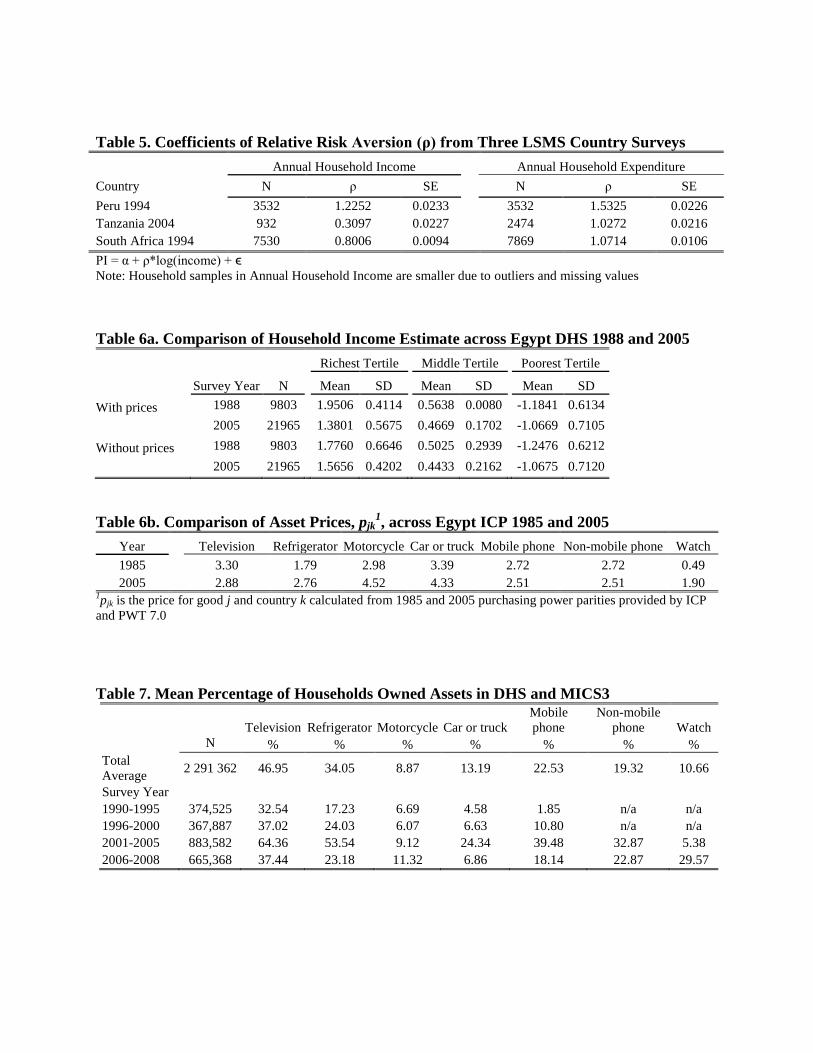
Table 5. Coefficients of Relative Risk Aversion (ρ) from Three LSMS Country Surveys

Annual Household Income Annual Household Expenditure

Country N ρ SE N ρ SE

Peru 1994 3532 1.2252 0.0233 3532 1.5325 0.0226

Tanzania 2004 932 0.3097 0.0227 2474 1.0272 0.0216

South Africa 1994 7530 0.8006 0.0094 7869 1.0714 0.0106

PI = α + ρ*log(income) + ϵ

Note: Household samples in Annual Household Income are smaller due to outliers and missing values

Table 6a. Comparison of Household Income Estimate across Egypt DHS 1988 and 2005

Richest Tertile

Middle Tertile

Poorest Tertile

Survey Year N

Mean SD

Mean SD

Mean SD

With prices 1988 9803 1.9506 0.4114

0.5638 0.0080

-1.1841 0.6134

2005 21965 1.3801 0.5675

0.4669 0.1702

-1.0669 0.7105

Without prices 1988 9803 1.7760 0.6646

0.5025 0.2939

-1.2476 0.6212

2005 21965 1.5656 0.4202

0.4433 0.2162

-1.0675 0.7120

Table 6b. Comparison of Asset Prices, pjk1, across Egypt ICP 1985 and 2005

Year Television Refrigerator Motorcycle Car or truck Mobile phone Non-mobile phone Watch

1985 3.30 1.79 2.98 3.39 2.72 2.72 0.49

2005 2.88 2.76 4.52 4.33 2.51 2.51 1.90 1pjk is the price for good j and country k calculated from 1985 and 2005 purchasing power parities provided by ICP

and PWT 7.0

Table 7. Mean Percentage of Households Owned Assets in DHS and MICS3

Television Refrigerator Motorcycle Car or truck

Mobile

phone

Non-mobile

phone Watch

N % % % % % % %

Total

Average 2 291 362 46.95 34.05 8.87 13.19 22.53 19.32 10.66

Survey Year

1990-1995 374,525 32.54 17.23 6.69 4.58 1.85 n/a n/a

1996-2000 367,887 37.02 24.03 6.07 6.63 10.80 n/a n/a

2001-2005 883,582 64.36 53.54 9.12 24.34 39.48 32.87 5.38

2006-2008 665,368 37.44 23.18 11.32 6.86 18.14 22.87 29.57

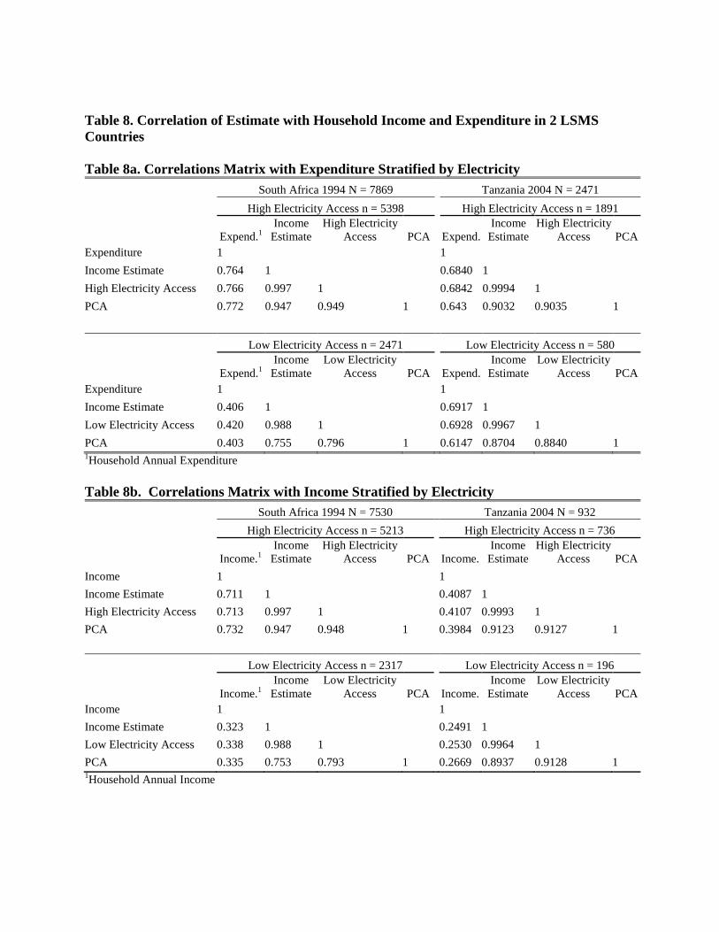
Table 8. Correlation of Estimate with Household Income and Expenditure in 2 LSMS

Countries

Table 8a. Correlations Matrix with Expenditure Stratified by Electricity

South Africa 1994 N = 7869 Tanzania 2004 N = 2471

High Electricity Access n = 5398 High Electricity Access n = 1891

Expend.1

Income

Estimate

High Electricity

Access PCA Expend.

Income

Estimate

High Electricity

Access PCA

Expenditure 1 1

Income Estimate 0.764 1 0.6840 1

High Electricity Access 0.766 0.997 1 0.6842 0.9994 1

PCA 0.772 0.947 0.949 1 0.643 0.9032 0.9035 1

Low Electricity Access n = 2471 Low Electricity Access n = 580

Expend.1

Income

Estimate

Low Electricity

Access PCA Expend.

Income

Estimate

Low Electricity

Access PCA

Expenditure 1 1

Income Estimate 0.406 1 0.6917 1

Low Electricity Access 0.420 0.988 1 0.6928 0.9967 1

PCA 0.403 0.755 0.796 1 0.6147 0.8704 0.8840 1 1Household Annual Expenditure

Table 8b. Correlations Matrix with Income Stratified by Electricity

South Africa 1994 N = 7530 Tanzania 2004 N = 932

High Electricity Access n = 5213 High Electricity Access n = 736

Income.1

Income

Estimate

High Electricity

Access PCA Income.

Income

Estimate

High Electricity

Access PCA

Income 1 1

Income Estimate 0.711 1 0.4087 1

High Electricity Access 0.713 0.997 1 0.4107 0.9993 1

PCA 0.732 0.947 0.948 1 0.3984 0.9123 0.9127 1

Low Electricity Access n = 2317 Low Electricity Access n = 196

Income.1

Income

Estimate

Low Electricity

Access PCA Income.

Income

Estimate

Low Electricity

Access PCA

Income 1 1

Income Estimate 0.323 1 0.2491 1

Low Electricity Access 0.338 0.988 1 0.2530 0.9964 1

PCA 0.335 0.753 0.793 1 0.2669 0.8937 0.9128 1 1Household Annual Income

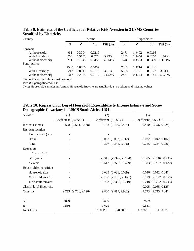
Table 9. Estimates of the Coefficient of Relative Risk Aversion in 2 LSMS Countries

Stratified by Electricity

Country Income Expenditure

N SE Diff (%) N SE Diff (%)

Tanzania

All households 961 0.3004 0.0219 2471 1.0402 0.0216

With Electricity 760 0.3101 0.025 3.23% 1889 1.0454 0.0258 1.24%

Without electricity 201 0.1543 0.0452 -48.64% 578 0.8863 0.0399 -11.31%

South Africa

All 7530 0.8006 0.0094 7869 1.0714 0.0106

With Electricity 5213 0.8311 0.0113 3.81% 5398 1.1071 0.0127 3.33%

Without electricity 2317 0.2028 0.0117 -74.67% 2471 0.3244 0.0141 -69.72%

ρ = coefficient of relative risk aversion

PI = α + ρ*log(income) + ϵ

Note: Household samples in Annual Household Income are smaller due to outliers and missing values

Table 10. Regression of Log of Household Expenditure to Income Estimate and Socio-

Demographic Covariates in LSMS South Africa 1994

N =7869 (1) (2) (3)

Coefficient (95% CI) Coefficient (95% CI) Coefficient (95% CI)

Income estimate 0.528 (0.518, 0.538) 0.432 (0.420, 0.444) 0.410 (0.396, 0.424)

Resident location

Metropolitan (ref) - - -

Urban - 0.082 (0.052, 0.112) 0.072 (0.042, 0.102)

Rural - 0.276 (0.245, 0.306) 0.255 (0.224, 0.286)

Education -

>10 years (ref) - - -

5-10 years - -0.315 (-0.347, -0.284) -0.315 (-0.346, -0.283)

<5 years - -0.512 (-0.556, -0.469) -0.513 (-0.557, -0.470)

Household composition -

Household size - 0.035 (0.031, 0.039) 0.036 (0.032, 0.040)

% of children < 15 - -0.130 (-0.188, -0.071) -0.119 (-0.177, -0.060)

% of adult females - -0.263 (-0.306, -0.219) -0.248 (-0.292, -0.205)

Cluster-level Electricity - - 0.095 (0.065, 0.125)

Constant 9.713 (9.701, 9.726) 9.860 (9.817, 9.902) 9.793 (9.745, 9.840)

N 7869 7869 7869

R2 0.566 0.629 0.631

Joint F-test 190.19 p<0.0001 171.92 p<0.0001

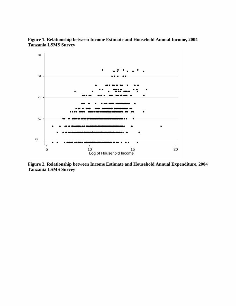
Figure 1. Relationship between Income Estimate and Household Annual Income, 2004

Tanzania LSMS Survey

-20

24

6

Wea

lth In

de

x

5 10 15 20Log of Household Income

Figure 2. Relationship between Income Estimate and Household Annual Expenditure, 2004

Tanzania LSMS Survey

-20

24

6

Wea

lth In

de

x

8 10 12 14 16Log of Household Expenditure

Figure 3. Relationship between Income Estimate and Asset Index by Principal Component

Analysis, 2004 Tanzania LSMS

-20

24

6

Wea

lth In

de

x

-5 0 5 10 15PCA

Figure 4. Relationship between Income Estimate and Household Annual Income from 1994

Peru LSMS Survey

-20

24

6

Wea

lth In

de

x

8 10 12 14 16Log of Household Income

Figure 5. Relationship between Income Estimate and Household Annual Expenditure from

1994 Peru LSMS Survey

-20

24

6

Wea

lth In

de

x

8 10 12 14Log of Household Expenditure

Figure 6. Relationship between Income Estimate and Asset Index by PCA from 1994 Peru

LSMS

-20

24

6

Wea

lth In

de

x

-5 0 5 10PCA

Figure 7. Relationship between Income Estimate and Household Annual Income from 1994

South Africa LSMS Survey

-2-1

01

23

Wea

lth In

de

x

7 8 9 10 11 12Log of Household Income

Figure 8. Relationship between Income Estimate and Household Annual Expenditure from

1994 South Africa LSMS Survey

-2-1

01

23

Wea

lth In

de

x

8 9 10 11 12Log of Household Expenditure

Figure 9. Relationship between Income Estimate and Asset Index by PCA from 1994 South

Africa

-2-1

01

23

Wea

lth In

de

x

-2 0 2 4PCA

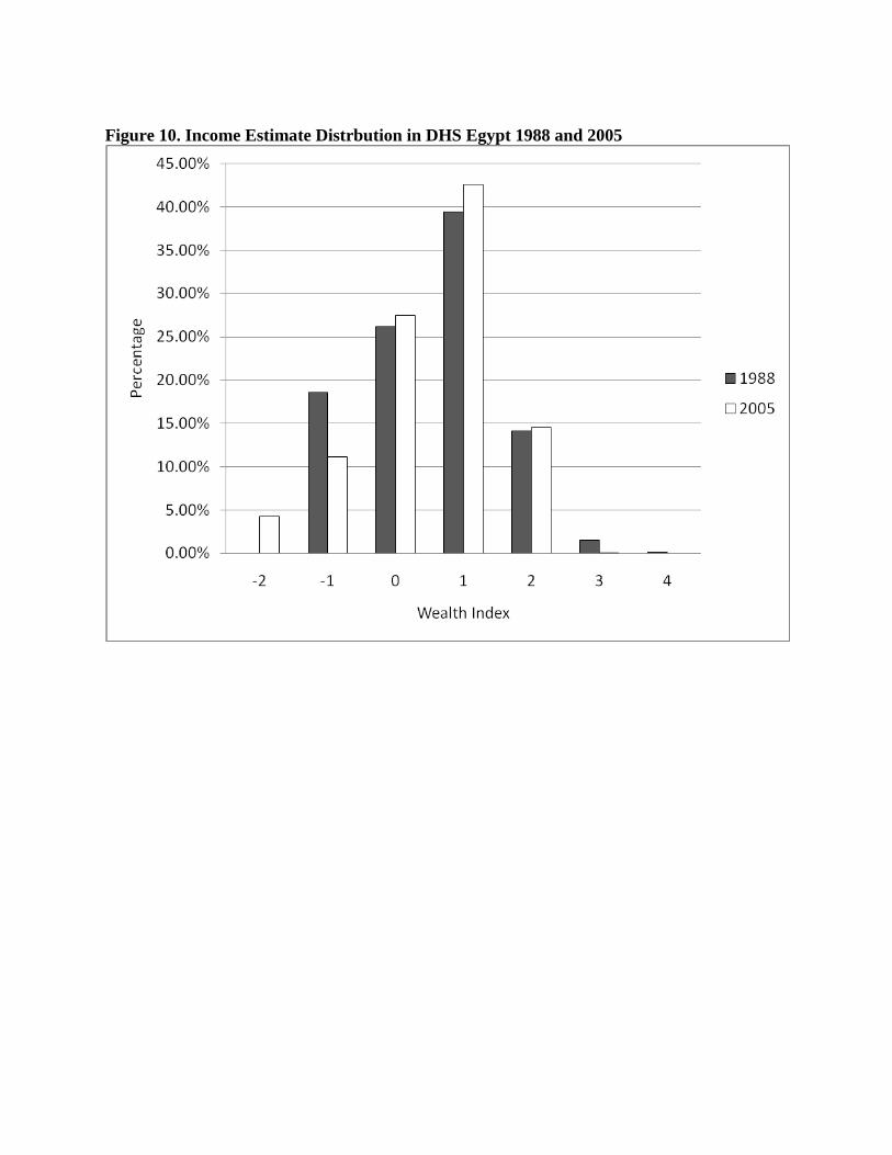
Figure 10. Income Estimate Distrbution in DHS Egypt 1988 and 2005

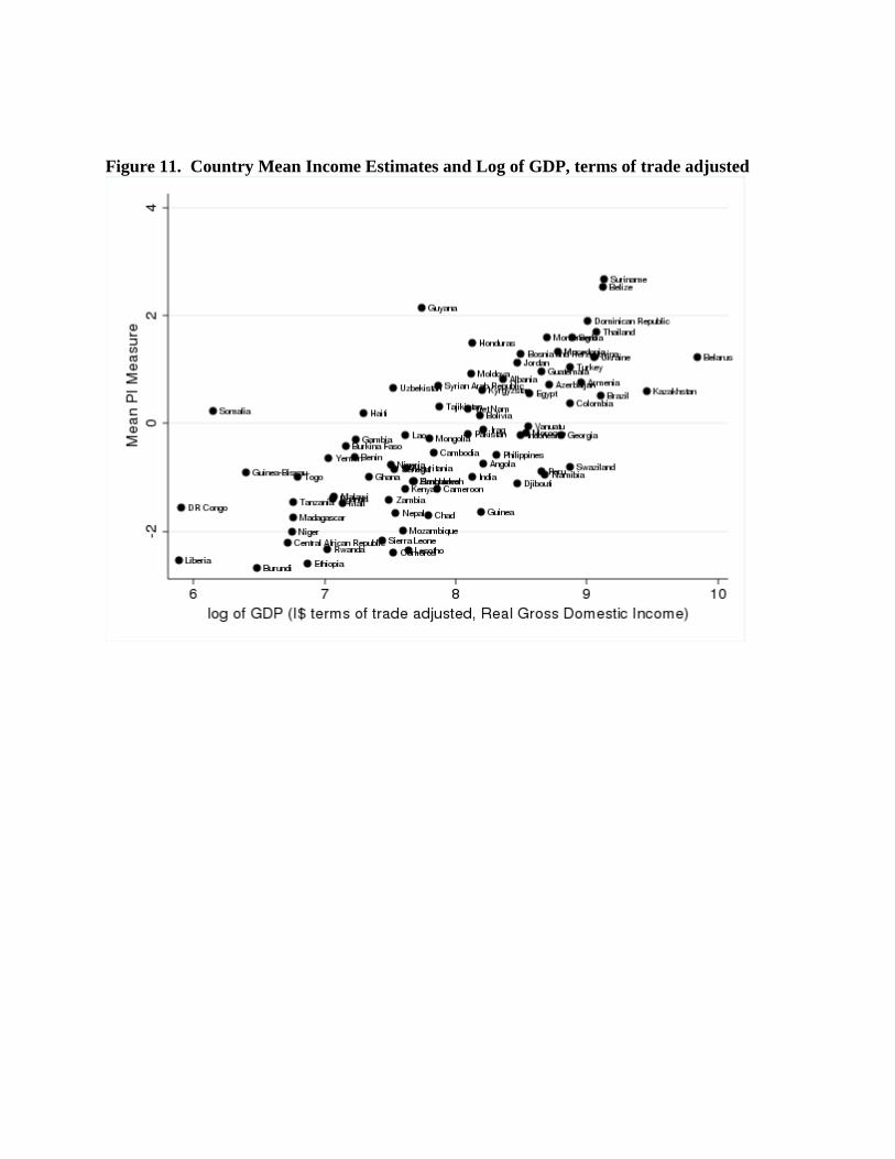
Figure 11. Country Mean Income Estimates and Log of GDP, terms of trade adjusted

H. APPENDIX

Table A1. Country Rankings by Indicators

Country Survey Year

Income

Estimate GDP HDI MPI MPI-LS

Burundi 2005 1 5 7 5 1

Ethiopia 2005 2 11 10 2 4

Liberia 2008 3 1 13 10 9

Comoros 1996 4 26 39 16 11

Lesotho 2004 5 33 24 39 19

Rwanda 2005 6 12 14 13 2

Central African

Republic 2006 7 6 4 7 8

Sierra Leone 2005 8 22 2 9 7

Niger 2006 9 7 1 1 6

Mozambique 2003 10 29 9 11 14

Madagascar 2008 11 9 33 14 18

Chad 2004 12 37 11 24 3

Nepal 2006 13 28 34 23 25

Guinea 2005 14 49 12 8 17

DR Congo 2007 15 2 6 17 16

Mali 2006 16 16 3 3 12

Tanzania 2007 17 8 25 21 10

Zambia 2007 18 23 17 25 24

Uganda 2006 19 14 21 - -

Malawi 2006 20 15 18 19 5

Republic of Congo 2005 21 - 42 36 29

Cameroon 2006 22 40 29 30 31

Kenya 2008 23 30 32 29 15

Djibouti 2005 24 56 28 47 52

Zimbabwe 2005 25 34 43 34

Bangladesh 2007 26 35 31 32 26

India 1992 27 46 41 31 38

Togo 2006 28 10 22 33 28

Ghana 2008 29 21 27 45 39

Namibia 2006 30 65 45 40 35

Guinea-Bissau 2006 31 4 8 - -

Peru 2003 32 64 72 50 44

Senegal 2008 33 27 16 18 40

Mauritania 2007 34 32 26 22 32

Swaziland 2006 35 70 38 41 33

Nigeria 2008 36 24 23 20 30

Angola 2006 37 51 35 12 20

Yemen 2006 38 13 37 34 45

Benin 2006 39 18 20 15 22

Philippines 2008 40 53 60 53 55

Cambodia 2005 41 39 40 38 23

Cote d'Ivoire 2006 42 - 19 27 47

Burkina Faso 2006 43 17 5 4 21

Gambia 2005 44 19 15 26 36

Mongolia 2005 45 38 53 54 43

Indonesia 2007 46 58 56 49 49

Georgia 2005 47 69 65 80 64

Lao 2006 48 31 43 37 37

Pakistan 2006 49 44 36 35 41

Morocco 2003 50 60 44 46 54

Iraq 2006 51 52 - 56 63

Vanuatu 2007 52 61 47 - -

Bolivia 2008 53 48 57 42 46

Haiti 2005 54 20 30 28 27

Somalia 2006 55 3 - 6 13

Viet Nam 2006 56 43 54 51 51

Tajikistan 2005 57 42 46 52 53

Colombia 2004 58 71 74 60 58

Brazil 1996 59 79 77 62 66

Egypt 2008 60 62 49 63 74

Kazakhstan 2006 61 83 73 81 71

Kyrgyzstan 2005 62 50 50 68 59

Uzbekistan 2006 63 25 51 71 67

Syrian Arab

Republic 2006 64 41 59 66 70

Azerbaijan 2006 65 67 62 65 65

Armenia 2005 66 74 70 72 75

Albania 2005 67 54 79 77 73

Moldova 2005 68 45 52 70 62

Guatemala 1998 69 63 48 48 42

Turkey 2003 70 72 75 61 60

Jordan 2007 71 57 64 69 81

Belarus 2005 72 84 80 82 82

Ukraine 2005 73 77 71 74 80

Bosnia and

Herzegovina 2006 74 59 76 79 78

Macedonia 2005 75 68 78 73 72

Honduras 2005 76 47 58 44 50

Montenegro 2005 77 66 81 75 79

Serbia 2005 78 73 82 78 77

Thailand 2005 79 78 69 76 69

Dominican Republic 2007 80 76 66 58 56

Guyana 2006 81 36 55 57 57

Belize 2006 82 81 68 64 61

Suriname 2006 83 82 63 59 68

Trinidad and

Tobago 2006 84 - 83 67 76

HDI: Human Development Index 2003; MPI: Multi-dimensional Poverty Index, varying years; MPI-LS: MPI Living

Standard score, same years as MPI; PWT: Penn World Tables estimates of real gross domestic income: GDP TT:

GDP terms of trade adjusted, 2005; Year: Year of the survey from which data were used to compare with GDP.

*The HDI value for Haiti is from 2006, as opposed to 2005 for all other countries.

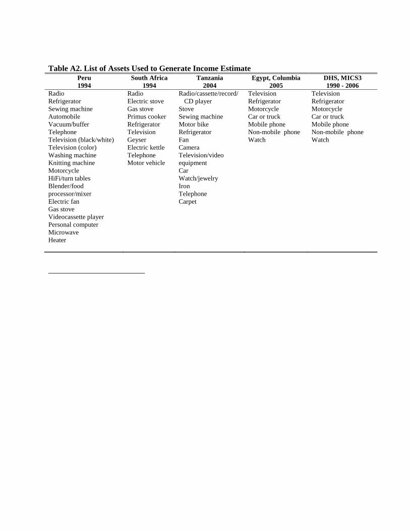
Table A2. List of Assets Used to Generate Income Estimate

Peru

1994

South Africa

1994

Tanzania

2004

Egypt, Columbia

2005

DHS, MICS3

1990 - 2006

Radio

Refrigerator

Sewing machine

Automobile

Vacuum/buffer

Telephone

Television (black/white)

Television (color)

Washing machine

Knitting machine

Motorcycle

HiFi/turn tables

Blender/food

processor/mixer

Electric fan

Gas stove

Videocassette player

Personal computer

Microwave

Heater

Radio

Electric stove

Gas stove

Primus cooker

Refrigerator

Television

Geyser

Electric kettle

Telephone

Motor vehicle

Radio/cassette/record/

CD player

Stove

Sewing machine

Motor bike

Refrigerator

Fan

Camera

Television/video

equipment

Car

Watch/jewelry

Iron

Telephone

Carpet

Television

Refrigerator

Motorcycle

Car or truck

Mobile phone

Non-mobile phone

Watch

Television

Refrigerator

Motorcycle

Car or truck

Mobile phone

Non-mobile phone

Watch