Essays on Monetary Policy

A c t a U n i v e r s i t a t i s T a m p e r e n s i s 945

U n i v e r s i t y o f T a m p e r eT a m p e r e 2 0 0 3

ACADEMIC DISSERTATIONTo be presented, with the permission of

the Faculty of Economics and Administration

of the University of Tampere, for public discussion in the

Paavo Koli Auditorium of the University, Kanslerinrinne 1,Tampere, on August 16th, 2003, at 12 o�clock.

PETRI MÄKI-FRÄNTI

Distribution

University of TampereBookshop TAJUP.O. Box 61733014 University of TampereFinland

Cover design byJuha Siro

Printed dissertationActa Universitatis Tamperensis 945ISBN 951-44-5716-1ISSN 1455-1616

Tampereen yliopistopaino Oy Juvenes PrintTampere 2003

Tel. +358 3 215 6055Fax +358 3 215 7685taju@uta.fihttp://granum.uta.fi

Electronic dissertationActa Electronica Universitatis Tamperensis 268ISBN 951-44-5717-XISSN 1456-954Xhttp://acta.uta.fi

ACADEMIC DISSERTATIONUniversity of Tampere, Department of EconomicsFinland

3

ACKNOWLEDGEMENTS

In the course of years of writing this doctoral thesis I have received help and assistance from many people to whom I would like to express my deepest gratitude. The burden of supervising my thesis project has actually been shared by four people (in alphabetical order): Professors Pekka Ahtiala and Kari Heimonen, Mr Hannu Kahra and Dr Jouko Vilmunen. Kari Heimonen, along with professor Juuso Vataja also acted as the off icial examiners of my thesis. I am deeply grateful for all of my supervisors for patiently reading and constructively criti cising my papers in the different stages of the study. I am also grateful to Markku Konttinen for his valuable assistance in my endless problems related to computers and Virginia Mattila for correcting my English. I owe a special thank to my colleagues Markus Lahtinen and Päivi Mattila-Wiro. Our numerous fierce debates on contemporary economic policy issues have, in addition to improving my argumentation skill s, also prevented me from getting isolated too high in the academic ivory tower. I have also received valuable comments, criti cism, suggestions and all sorts of assistance from many other people working in the Department of Economics in the University of Tampere. Thanks to all ! The study was mostly carried out during my appointment as a graduate school fellow on the Finnish Postgraduate Programme in Economics. Not to even mention the importance of the opportunity to concentrate on research full -time, the workshops and courses organised by the FPPE also have provided me with valuable intellectual stimulation during these years. Financial support has also been provided by the Yrjö Jahnsson Foundation, the Okobank Research Foundation and the Association of Professors and Docents. The Department of Economics in the University of Tampere has provided me with the necessary working faciliti es and a working room. I wish to express my thanks for all this support. I am also indebted to my friends living in Helsinki. Without the accommodation provided by them I would scarcely have got my FPPE courses finished at the beginning of my graduate studies. I would also like to thank all my non-economist friends for reminding me about li fe outside economics. Finally, I would like to thank my parents, who have encouraged me to finish the thesis even during the days when I wondered about the ultimate sense of the project. Tampere, June 2003 Petri Mäki-Fränti

4

Table of Contents Chapter 1 – Introduction 5 Chapter 2 – The Transmission of Monetary Policy Shocks between Two Countries 29 An Empirical Study with A Structural VAR Model Chapter 3 – The Regime Shifts in the Reaction Functions of the Federal 82 Reserve and the Bundesbank Chapter 4 – Should the ECB Adopt an Explicit Exchange Rate Target? 133 Chapter 5 – The Information Content of the Divisia Money in Forecasting the 181 Euro Area Inflation

5

CHAPTER 1

1. INTRODUCTION

“ Having looked at monetary policy from both sides now, I can testify that central banking in

practice is as much art as science. Nonetheless, while practising this dark art, I have always

found the science quite useful.” –Alan S. Blinder

1.1 Transmission mechanisms of monetary policy

The integrated world economy has become increasingly dependent on the monetary policy of

the two largest central banks, the Federal Reserve and the European Central Bank. Rises and

cuts in the short-term interest rates are quickly transmitted to all sectors of the national

economies through the changes the short rates induce in the prices of other assets li ke bonds,

stocks and exchange rates. The importance of monetary policy has further increased due to the

diminished slack of f iscal policy and the practical diff iculties to successfully conduct

stabili zing fiscal policy. Recent discussion about the role of the central bank has even touched

upon such issues like should the central bank also be interested in stabili sing the asset market

or exchange rate volatilit y.

The four essays of the dissertation take both positive and normative viewpoints to some of the

many still open problems in monetary policy and monetary economics. The essays touch upon

quite a wide variety of issues, such as the nature of the transmission mechanism of monetary

policy, a correct variable set the central bank should look at when making its policy decisions

as well as some empirical analysis of the behaviour of the Federal Reserve and the German

Bundesbank after the collapse of the Bretton-Woods system.

Between the collapse of the Bretton Woods system at the beginning of the 1970’s and the

present day, a vast body of literature concerning the abilit y of a central bank to affect inflation

and output has emerged. Some extreme approaches – the rational expectations literature and

the real business cycle literature – have actually gone as far as to state that the monetary policy

6

actions would have littl e or no effect on the real economy. Particularly along with the common

acceptance of the existence of price and/or wage rigidities affecting the economies, these

extreme views seem to have vanished, however.

Some kind of consensus view about the possibilit y of unexpected monetary policy shocks to

affect economy can be found e.g. in Walsh (1998), who reviews recent empirical lit erature on

both short-run and long run relations between money, inflation and output. According to

Walsh, in the long-run there is a correlation of almost unity between money growth and

inflation, while the correlation between money growth and real output seems to be close to

zero, or even negative for high inflation countries. In the short run there is still some role for

fine-tuning however, since an exogenous monetary policy shock seems to result in hump-

shaped responses in the real output. It takes several quarters before the maximum response is

reached, after which the output converges to its initial level. In the case of effects of the

systematic monetary policy operations, no strong consensus can any longer be found,

however, although e.g. the large structural econometric model used by the Federal Reserve

provides qualitatively largely similar responses to short-term interest rate rises than do the

VARs1.

When it comes to the structural interpretations of these empirical regularities, in addition to

the interest rate channel, one can list numerous transmission channels to monetary policy, such

as the exchange rate channel, equity price channels, the wealth channel, the bank lending

channel and the balance sheet channels. Walsh (1998) classifies the currently dominating

modelli ng strategies in monetary economics into three broad main approaches; the

representative agent models, the overlapping generations models and the models that are based

more on ad hoc assumptions than on the behaviour of optimising agents.

The roots of the new open economy macroeconomics lie in the seminal papers by Obstfeld

and Rogoff fr om the middle of the nineties2. Obstfeld and Rogoff extended the closed

economy macroeconomic models based on solid microeconomic foundations to cover also the

problematic of the open economies. Nominal rigidities and market imperfections either in

product or factor markets are the key assumptions needed to ensure a role for monetary policy

in these models. Since the models are based on the behaviour of optimising agents, they allow

for the explicit welfare analysis, which is a clear advantage when compared to the traditional

1 Walsh (1998), p.35. 2 See e.g. Obstfeld and Rogoff (1995, 1996)

7

Mundell -Fleming models. Despite many of the desirable properties of the new open economy

macromodels, there is still one important restrictive shortcoming related to them, namely the

sensitivity of the basic results of the models on the exact assumption of the models. This

makes the models somewhat problematic also from the point of view of practical policy

making3. Thus, there still seems to be a role for the traditional ISLM type of models as

workhorse models in practical monetary policy analysis.

In light of this, an interesting contribution to the practical monetary policy analysis has been

the so-called New Keynesian models that combine the simplicity of the traditional ISLM

models with solid microeconomic foundations. A typical New Keynesian model consists of a

simple monetary policy rule, a forward-looking IS-curve representing the demand side and a

Philli ps-curve representing the supply side of the economy. In further contrast to the

traditional ISLM-Philli ps curve analysis, not only the IS curve, but also the Philli ps curve is

often modelled as forward looking. The New Keynesian models differ from the traditional,

static ISLM models also in that the models are dynamic, stated in terms of difference

equations and the both the IS curve and the Philli ps curve are derived from the behaviour of

optimising agents.

The international transmission mechanisms of monetary policy are dealt with in the first of the

essays in Chapter 1. The essay examines empirically the transmission of unexpected monetary

policy shocks between the US and Europe, using a simple structural vector autoregression

(SVAR) model. The relevance of the research problem of the first essay of the dissertation

hinges on the relative importance of the unexpected monetary policy shocks, compared to the

anticipated monetary policy actions. An even more important problem addressed in the essay

is how to correctly identify the unexpected shock component of the monetary policy in an

open economy. In the closed economy context, the identification of the monetary policy

shocks can be based on a simple Choleski decomposition, which assumes that the variables of

the model are solved recursively so that the short interest rate (the policy instrument) cannot

affect the other model variables, but the other variables can affect the interest rate. In the open

economy context such a recursiveness assumption is no longer valid if the model includes

variables like exchange rates that are contemporaneously connected to each other by the

3 Lane (2001)

8

central bank’s policy variable. Thus, more structural approaches for setting the identifying

restrictions between the model variables are called for.

Despite the favourable properties of the new open economy macromodels, it is quite diff icult

to derive a set of identifying restrictions to use in SVAR modelli ng4. Hence, the theoretical

framework behind the identification scheme of the first of the essays is still characterized by

the ISLM tradition. On the other hand, when interpreting the results, some insights have also

been sought from the new open economy macroeconomics discussed above. Some of the

results in particular contradict the traditional beggar-thy-neighbour view of the domestic

effects of the depreciating currency were diff icult to explain in the ISLM framework. In

general, the results are however in line with the results obtained in previous studies about the

effects of monetary policy shocks.

The most important results of Chapter 1 are as follows: After a negative US monetary policy

shock, the outputs of both countries decline, which contradicts the beggar-thy-neighbor result.

The nominal USD appreciates against the DEM and the long term interest rates decline. The

effects of the German monetary policy shock closely resemble the US results above. The

outputs of both countries still seem to decline in both countries, but surprisingly, the output

effect of a monetary policy shock is greater from Germany to the US than the other way

round. The DEM appreciates and the long term interest rates react with an initial rise, after

which they fall .

4 Antipin and Luoto (2001) provide, however, an example of SVAR studies where the identifying restrictions are derived from a macromodel with optimising agents.

9

1.2 The goals of monetary policy and the Taylor r ule

Whether the conduct of monetary policy is a purely technical matter, or whether a politi cal

point of view should be reflected in the decision-making of central banks is still an open

question. The role of the central banks has been more or less increasing for the whole century,

but the tendency has been as its strongest during the past fifteen years, while the preferences

of public opinion have also turned more and more to favour anti-inflationary monetary policy.

It was originally demonstrated by Barro and Gordon at the beginning of the 1980s that an

independent central bank may have an important role guaranteeing the success of anti-

inflationary monetary policy5. Barro and Gordon suggested that an independent central bank,

perhaps even following a strict, mechanistic rule, would provide an eff icient solution to the

well -known time-inconsistency problem stemming from the politi cians’ attempts to make use

of the short-run Philli ps curve to achieve electoral gains6.

Whether a mechanistic policy rule provides a more eff icient outcome in monetary policy than

discretionary actions has been under debate. While a mechanistic policy rule would provide

transparency and predictabilit y for consumers, job markets and financial markets, the absence

of stable causal li nks between the monetary policy instruments, inflation and income makes

their use questionable. Unexpected macroeconomic events in particular, such as the stock

market crash of October 1987 or the surge in the US productivity in the latter half of the 1990s

inevitably call for flexibilit y in decision-making7. In addition, the role of a rigid policy rule in

providing a shield against politi cal pressure may not be relevant, at least in most of the

developed world. As the disinflationary tendency in the industrialized world, beginning in the

1980’s has shown, the central banks in these countries have in fact tended to avoid the Barro-

Gordon bias. As Svensson (2002a) and Blinder (1999) have argued, this follows simply from

the fact that after all , although the central banks have paid some attention to stabili sing output,

they still have succeeded in not pursuing overambitious output targets.

Although there always seems to be a need for discretion in actual monetary policy-making,

rule-like behaviour may be a practical way to summarise some observed key regularities in

5 See Barro and Gordon (1983a, 1983b) 6 Barro’s and Gordon’s views on the existing inflationary bias in the central bankers’ preferences has been criticized interestingly by Blinder (1999, Ch. 2.) 7 For a discussion on examples of successful, highly discretionary monetary policy decisions, see Greenspan (1997) and Mankiw (2001).

10

central bank behaviour. Also the essays of Chapters 2, 3 and 4 of this dissertation are at least

implicitl y based on estimating or specifying such a rule. Perhaps the best known example of

simple monetary policy rules is the Taylor rule (see Taylor 1993), according to which the

central bank should set the short interest rate by responding to deviations of both inflation and

output from their desired target levels8.

Originally, the Taylor rule was found to match the US interest rate series well , but since its

invention, the rule has become a popular tool for modelli ng the essential features of the

behaviour of central banks all over the developed world. The performance of the rule has also

turned out to be robust for the choice of the model characterising the monetary transmission

mechanism. These characteristics include for instance, whether the monetary policy is

transmitted through the financial market prices or the credit channel, whether the model is

backward looking or forward looking, whether the exchange rate plays a role in the

transmission mechanism or not, or how the nominal rigidities are modelled9. The second

advantage of the instrument rules like the Taylor rule is its simplicity and transparency, which

also makes it an eff icient tool of communicating the central banks’ strategies10 11.

An alternative approach to instrument rules like the Taylor rule as a basis for monetary policy

would be forecast targeting – that is, setting the instrument variable of the monetary policy in

a way that makes the central bank’s conditional forecasts for its target variable(s) inflation

(and output) reach their chosen target values. This is an approach promoted by Lars E. O.

Svensson. In practice, forecast targeting means just inflation targeting, and in line with this

approach, some countries, li ke UK and Australia have followed the initial example of New

Zealand in 1990 and started to cast their monetary policy objectives simply in terms of a an

explicitl y stated inflation target. The advantages of the forecast targeting approach over the

simple decision rules is, first, that the former takes into account a large set of information,

whereas the Taylor rule contains only a small subset of the information available. Secondly, if

8 Since the SVAR modelli ng exercise of Chapter 2 focuses on the unexpected part of the monetary policy, the underlying policy rules of these models can be characterized as a central bank reaction function in surprises, as opposed to the Taylor rule in the strict sense of the word, which is more concerned with the systematic part of the monetary policy. See Clarida (2001), p .3. 9 See Taylor (1999) 10 See eg King (1999), p. 24 11 The Taylor rule has sometimes been associated with credibilit y problems, since there are no mechanisms that would actually bind the policymaker to follow the rule. This criticism is not very convincing, after all . Instead of being a rigid, mechanical rule to be followed blindly, the Taylor rule provides a simple tool for summarising the main cyclical developments of the economy for use in connection with other information sources.

11

followed too mechanistically, the rules do not allow the extent of discretion often necessary in

practical policymaking.

According to Svensson (2002a, pp. 2), the strategy of inflation targeting is defined by three

characteristics: At first, the inflation target can be expressed numerically, either as a target

range or as a point target. Secondly, the decision-making process is based on the central

bank’s inflation forecast. Thus, when setting the stance of the monetary policy, the inflation

forecast should be consistent with the inflation target. Thirdly, the monetary policy should be

transparent and accountable. Allsopp (2001) in turn, highlights the last of the criteria by

pointing out that if inflation targeting is to be successful, the monetary policy should stabili se

expectations of the markets concerning both the inflation and growth.

Despite its popularity, neither the Fed nor the ECB has defined their strategies in terms of pure

inflation targeting. The ECB rests on its famous two-pill ar strategy, consisting of a

quantitative definition for price stabilit y, augmented by a reference value for the growth rate

of M3 money and a broadly based assessment of the outlook for future price developments in

the Euro area. According to the Maastricht Treaty, the ECB should also pursue other

objectives like high employment, but only as long as it does not interfere with maintaining

price stabilit y, the primary objective of the ECB. The Fed, in turn, does not have any explicitl y

stated monetary policy strategy at all , although in the Federal Reserve Act the bank has been

given the mandate of promoting “ the goals of maximum employment, stable prices and

moderate long-term interest rates” . On the other hand, it has been argued that in practice the

Fed (and the German Bundesbank before the birth of the ECB and common monetary policy),

pursued a monetary policy close to formal inflation targeting12.

Even if the inflation targeting central bank’s target was expressed entirely in terms of

inflation, the central bank can still also put some weight on stabili sing the output gap. The

positive weight to the output gap under an inflation targeting regime can be motivated on two

grounds. At first, the output gap may have positive weight in the inflation targeting central

bank’s loss function. If the output gap is given some explicit weight in the inflation targeting

central bank’s loss function, the inflation regime is often called “ flexible”, or “constrained”

inflation targeting. On the other hand, even if the explicit weight put on the output gap target

12 See e.g. Mishkin (1999, 2002).

12

in the central bank’s welfare function is zero (“ the inflation nutter” case), the optimal policy

still calls some attention to be paid to stabili sing output because of the information content that

the output gap may include about the future inflation. 13

What the optimal long-run target value for inflation should be, is still an open question.

Despite their anti-inflationary preferences, it is not typical for any central bank, even the

inflation targeters, to strictly follow the so-called Friedman rule14, which states that the social

optimum is achieved if the inflation target is set simply at zero. There are two classic

arguments in favour of a small positive inflation target. At first, if there is some inflation in the

economy, some flexibilit y for the real wages can be obtained even in the case of short-run

wage rigidities present, as originally put forward by Akerlof, Dickens and Perry (1996). While

at least with the US data the empirical evidence leaves the degree of downward rigidity of the

nominal wages an open issue15, there still remains the second argument that is more diff icult

to refute: With a positive inflation rate, the zero bound for nominal interest rates prevents the

central bank from achieving a negative real interest rate. This makes boosting the economy

under recession a diff icult, if not completely impossible task16. Moreover, during episodes

with falli ng prices, there is the danger of the economy falli ng into “debt deflation” , as

originally proposed by Fisher (1933).

In this dissertation, questions related to the monetary policy rules are discussed explicitl y in

Chapters 3 and 4. The sort of VAR modelli ng exercise of the first essay in Chapter 2 was

implicitl y based on an assumption of a policy rule with stable parameter values over time. The

relevance of this assumption is discussed in the second of the essays (Chapter 3), which

estimates Markov regime switching models for the Taylor-type monetary policy rules of the

Bundesbank and the Fed to detect possible structural changes in the parameters of the rules.

Although empirical macroeconomic modelli ng seems to favour linear models, the non-linear

models, such as Markov Switching, TAR or STAR models seem to gain popularity in

modelli ng financial time-series like interest rates.

13 For a discussion on the output stabili cation objective of inflation targeting central banks, see e.g. Svensson (2002b). 14 Friedman (1969) 15 For a discussion, see Mishkin – Schmidt-Hebbel (2001), p. 27. 16 Of course, the estimated positive responses to the output gap by the central banks could be interpreted only as reactions to the information content of the output over the future inflation trends. Clarida et al. (1998) however, provide empirical evidence according to which the output gap seems to have been included in the reaction functions of the G3 central banks.

13

Chapter 3 extends the previous literature on estimated policy rules of the Fed and the

Bundesbank firstly, in that our non-linear econometric model allows for endogenizing the

timing of the possible structural changes. It has been typical for the previous studies17 on the

subject to assume that the dates of these breaks are known a priori. The second contribution of

the study was to shed further light on the debate on the robustness of the estimated Taylor type

policy rules on the exact definitions of the output gap and inflation.

According to the results of Chapter 3, the policy rules of the Fed and the Bundesbank have

experienced notable structural changes during the sample period, although the interpretation of

the structural breaks was not always easy. In light of this finding, the results from our first

essay should also be interpreted with caution, although the structural stabilit y of the equations

of the SVAR model was tested. Some additional evidence was also found supporting the

views of Orphanides (2001), Kozicki (1999) and Cerra et al. (2000) that the empirical

estimates of the Taylor rule may be significantly sensitive on the exact specification of the rule

and the data used in the estimations.

Chapter 4 studies whether the ECB should start to stabili se the exchange rate of euro. The

original motivation for the research problem was based on the sharp depreciation of the euro

against the US dollar that the euro faced after its launch in 1999, which on the other hand has

turned into a marked appreciation after the the essay was completed. The study discusses the

desirabilit y of an exchange rate target for the ECB both from the viewpoint of the whole union

and from that of a single member state. Thus, for its part the study extends the literature on the

optimal currency areas.

The way the central bank should react to exchange rate changes ultimately depends on the

nature of the exchange rate shocks. Consider, for instance, depreciation of the currency. If the

depreciation stems from pure portfolio shocks, the depreciation is li kely to raise inflation,

which calls for higher interest rates. If the depreciation, however, results from real shocks, the

optimal response of the central bank may be as well ti ghtening or loosening the monetary

policy, depending on the exact nature of the shock. For example in the case of a negative

terms-of-trade shock, which lowers aggregate demand through reducing demand for exports,

17 See e.g. Judd and Rudebusch (1998), Clarida and Gertler (1996) and Clarida et al. (1998)

14

deflation is a more likely outcome than inflation and therefore lower, rather than higher

interest rates are needed.18

Rogoff (2001), in turn, argues in terms of a theoretical model that because of trade friction,

both the global goods and capital markets are much less integrated than is commonly believed.

It follows that in a highly segmented goods market, only a small change in fundamentals is

needed to create large but fully rational changes in the exchange rate. In addition, the changes

in the exchange rate have much less feedback to the real economy than is usually expected.

What might then have been the ultimate factors driving the exchange rate of the euro since its

launch at the beginning of 1999? The causes for the rapid depreciation of the euro after its

introduction have been examined empirically by de Grauwe (2000). The study actually fails to

find any stable link between the fundamentals and the euro/USD exchange rate during the

sample period. Instead, the euro/USD rate seems to have been driven by the investors’

expectations19 so that the marked weakening of the Euro rather resulted from more or less

irrational behaviour among investors than from the productivity differences between the US

and the euro area. Thus, the evidence was more in favour of pure portfolio, rather than real

shocks. If de Grauwe’s reasoning is correct, one consequence is that the effects of the central

banks’ interventions may be weaker than commonly believed, since the investors’

expectations become more diff icult to influence.

The previous empirical evidence on the role of the exchange rate in the policy rules of the

largest central banks include Clarida et al. (1998). According to the results, the central banks

of Germany and Japan seem to have reacted to deviations in their nominal exchange rates

against the US dollar from purchasing power parity, although the reaction has been small .

When interpreting this result, there are, however, the same problems present as when

interpreting the estimated positive weight put on the output gap, since there might be

diff iculties to separate the case of the nominal exchange rate included in the policy rule from

the case where the central bank has reacted only on the information that the exchange rate

18 See Mishkin and Schmidt-Hebbel (2001). 19 According to de Grauwe's reasoning, there is a great uncertainty among investors about the relation between the exchange rates and fundamentals. Because of this uncertainty, the exchange rate movements themselves “ frame” the investors’ beliefs of the fundamentals of the economies. Using these frames, agents tend to concentrate on looking only at those economic fundamentals that can corroborate their initial perception of the fundamental strength of the economy. This process can continue until the discrepancy between the investors’ beliefs and reality grows too large and the agents have to find another fundamental to look at.

15

contains onfuture inflation20. A special emphasis in Chapter 4 is put on the viewpoint of a

small union member state with a more open national economy and asymmetric business cycles

compared to the rest of the union. Thus, the study also contributes to the literature on optimum

currency areas (OCA), originating in the seminal paper by Mundell (1961). The goal of the

OCA literature is to compare the benefits that a country achieves by joining a currency union

against the costs from losing the opportunity for independent monetary and exchange rate

policies.

Beginning from the 1970’s this literature has focused particularly on the problem of how to

adjust to asymmetric economic shocks facing the member states of a monetary union. In the

case of asymmetric shocks, the one-size-fits-all monetary policy of the common central bank

of the union may no longer suit all the member states. The timing and magnitude of the effects

of the monetary policy may also differ among the member states if they have different

financial structures and wage-price processes. If the member states also differ from each other

in their degree of openness against the world outside the union, the exchange rate will play

larger role in the monetary transmission mechanism of the more open countries. Thus, for

these countries, exchange rate adjustments could provide a shield for the economic shocks that

is lost when joining a monetary union. If there are no other effective adjustment mechanisms

like trade linkages, high factor mobilit y or automatic fiscal stabili sers, the increased

adjustment costs for the economic shocks may greatly outweigh the benefits from the union.

The degree of asymmetry of the shocks facing the member states of the EMU has been

examined e.g. by Bayoumi and Eichengreen (1992, 1996). In both papers the authors find a

core group of countries with more highly correlated structural shocks than is faced by the

periphery group. As originally put forward by Kenen (1969), the shocks facing the regions of

the union are magnified if the manufacturing sectors of the economies are well diversified.

Krugman (1993), however, argues that after monetary unification, factors such as scale

sensitivity of production or reduced transportation costs may actually decline the

diversification of the production structures of the member countries. According to Mongelli

(2002) the production structures of most EU countries seem to be highly diversified, however.

On the other hand, Tavlas (1994) argues that the empirical evidence available seems to give

contradictory answers regarding the problem of symmetry. In Chapter 4 the covariance

20 See Clarida (2001).

16

structure of the shocks facing the member country is estimated with the Finnish data. In this

case, major asymmetries were found and they turned out also to be economically significant.

The previous empirical evidence on the differences in the transmission mechanisms between

the EMU member countries has been reviewed e.g. by Elbourne et al. (2001) and Dornbusch

et al. (1998). Elbourne et al. focus on reviewing the evidence provided by the previous VAR

studies, while Dornbusch et al. considers a wider array of models, including e.g. large

econometric models used by central banks. Both of the papers point out that the previous

findings on the monetary mechanism in Europe are sensitive to the selection of the

econometric model. At least Dornbusch et al. (1998) concludes however that due to the

differences in the labour markets and financial structures, evidence can be found supporting

significant differences in the monetary transmission mechanisms of the member states.

Although the OCA literature serves as a workhorse approach in analysing the different aspects

of monetary unions like EMU, the approach can still be criti cised. Part of the criti cism stems

from the discussion concerning the ultimate nature of the determination of the exchange rates.

If the exchange rates are mostly driven by portfolio shocks and if are even prone to speculative

bubbles, then they no longer provide an eff icient tool of adjustment. Accordingly, a stable

exchange rate introduced by the union in fact means a welfare gain in terms of reduced

uncertainty and lower interest rates. In addition, it may be argued that the different OCA

criteria to be met ex ante – symmetric shocks, openness, factor mobilit y, fiscal federalism –

may in fact be endogenous variables. That is, the financial structures and labour markets may

adapt themselves to the new environment created by monetary union.

The theoretical model used in Chapter 4 represents the so-called new normative

macroeconomic research that has rapidly gained popularity in the field of applied research on

monetary policy rules, both among academics and central bank research departments21. It is

typical of these models that they combine features from both the traditional ISLM type of

analysis, as well as from the models of the new open economy macroeconomics. The

traditional ISLM models perhaps lack solid microeconomic foundation, but as simple and

tractable models that often fit the data fairly well , they still serve as useful workhorses, at least

for applied researchers. In short, the basic idea behind the new normative macroeconomic

21 For discussion on such models, see Clarida et al. (2001) and McCallum (1999)

17

research is to calibrate, solve and simulate small macroeconomic models that consist of a

simple monetary policy rule and a set of equations describing the rest of the economy.

The results of Chapter 4 suggest that monetary union as a whole does not seem to benefit from

an exchange rate target, but the ECB’s attempts to stabili ze the exchange rate of the euro may

reduce particularly the volatilit y of output of the single member country with a more open

economy than the union on average. On the other hand, our simulations revealed that the

asymmetries in the business cycle pattern rather than the asymmetries in the structures of the

economies, may after all be a more important source for the poorer performance of the

member state. Thus, the conclusions of Chapter 4 of the dissertation are broadly in line with

the OCA literature.

1.3. The role of money in monetary policy

Beginning from the introduction of the quantity theory of money, money has been given a

prominent role in economists’ thinking about the transmission mechanisms of monetary

policy. However, in the recent discussions on the optimal design of monetary policy, it has

been taken for granted that targeting the short-term interest rate instead of some monetary

aggregate provides the nominal anchor for the monetary policy. Indeed, after the monetaristic

experiments in the US and in the UK at the turn of eighties, the interest rate has almost

completely displaced the monetary aggregate as central banks’ instrument variable. The debate

for and against using some monetary aggregate as the policy instrument of a central bank can

be organised around two necessary conditions that would have to be fulfill ed in order for

monetary targeting to be a viable strategy for a central bank. At first, there has to exist a stable

money demand relationship. Secondly, the money supply has to be an exogenous variable, that

is, it has to be controllable by the monetary authority.

The first of the conditions is related to Poole’s famous analysis (Poole (1970)). According to

Poole, if the shocks facing the economy mostly come from the real side of the economy, then

the monetary aggregates would actually serve best as the central bank’s target variables. If,

however, the shocks originate more from the money markets, then the interest rate would be

the best instrument. Intuitively, the first of the conditions can be explained by the fact that

with large velocity shocks in the money demand present, the relationship between money and

18

the goal variables of the monetary policy, li ke the GDP, does not hold. Failure to estimate a

stable money demand function points out to the breakdown of the relationship between the

monetary aggregates and the goal variables at least in the US case, although in the case of the

ECB the numerous recent attempts to estimate an EMU wide money demand equation have

been more promising22. The evidence concerning the second necessary condition, the

endogeneity of broad monetary aggregates such as M2 and M3, in turn, seems at least

unclear23. All i n all , the uncertainties regarding the two necessary conditions above have led

the policymakers to universally adopt the short-term interest rate as their target variable.

Although monetary aggregates would be useless as instrument variables for the central banks,

they may still serve as valuable indicators for future inflation. Even this role for money that

still depends on the degree of stabilit y of the underlying money demand relationship has

recently been under debate however24. According to a recent empirical study by de Grauwe &

Polan (2001), for example, even the long-run relation between inflation and the growth rate of

money seems to break down for low inflation countries. King (2002) however criti cises such

literature as “ tyranny of regressions” , that is, it relies excessively on simple reduced form

econometric models instead of more structural econometric models. On the other hand,

Meltzer (1999) examines a number of deflationary episodes of monetary history and, even

relying on the simple regression, succeeds in finding evidence that the interest rate did not

fully represent the monetary transmission process during those periods.

Allan H. Meltzer and Mervyn King have recently argued that there may be important channels

other than the short-term interest rate through which monetary policy affects real activity25.

They argue that economists should reconsider the possibilit y that, controlli ng for the role of

the short real interest rate, money may have an independent role in the transmission

mechanism of monetary policy through its effects on other asset prices than the short interest

rate. Theoretical motivation for the link between the money and asset prices could be based on

the idea that, in contrast to the assumptions of traditional finance theory, the equili brium

yields of the different assets may not be perfect substitutes and, accordingly, there may be

supply effects on financial yields. The supply effects are seen particularly in the risk premia of

22 See e.g. Friedman and Kuttner (1996) and Estrella and Mishkin (1997) on the money demand of the Fed. The stabilit y of money demand in the euro area is discussed in Kontolemis (2002). 23 See Mishkin (1999), p. 13. 24 For a discussion, see also Blinder (1999). 25 See Meltzer (1999) and King (2002).

19

the yields (King (2002), p. 171). Further, King (2002) suggests that increase in the quantity of

money in the economy may reduce the transaction costs due to frictions in the financial

markets, and thus affect the financial yields. Accordingly, an increase in the supply of money

makes investors reallocate their entire portfolios of assets, which then contributes to aggregate

demand. Transaction costs also play a role in Nelson (2002), in which introducing portfolio

adjusting costs to a general equili brium model makes the long-term interest rate a relevant

opportunity cost variable in the model. The presence of the long-term interest rate then

strengthens the link between nominal money and real aggregate demand in the model. Nelson

(2002) also examines the link between base money and output empirically, finding indeed

evidence about a positive link between them.

Even in the face of the above reasoning supporting the role of money in the economy, the

emphasis that the central banks put on simple sum monetary aggregates can be called into

question however, since these monetary aggregates do not appropriately take into account the

differing degree of liquidity of their component assets. One solution to both the theoretical and

empirical criti cism of the traditional monetary aggregates is provided by the Divisia monetary

aggregates, originally developed by Barnett (1980). The concept of Divisia money is based on

the idea that the monetary aggregates should be weighted averages over their components so

that the weights take into account the different degrees of liquidity of the component assets.

Although the long-run neutrality of money implies that when the forecast horizon is extended,

the forecasts based on the Divisia money and the simple sum money are likely to converge, it

would be expected that because of its favourable theoretical properties, the Divisia monetary

aggregates may include valuable additional information about the short-run inflation pressures

in the economy.

The last of the essays in Chapter 5 of the dissertation discusses the potential role of the Divisia

money as a potential indicator variable for the future inflation for the ECB. The exact research

problem of the study is to examine the relative information content of the Divisia M3 money

in predicting the euro area inflation dynamics, compared with the information content of the

simple sum M3 money. The empirical method used in the study is simulated out-of-sample

forecasting. Because of the better theoretical motivation, Divisia monetary aggregates offer a

tempting alternative for simple sum M3 as a source of information for future inflation in the

euro area. Although it is the growth rate of the nominal money that the ECB is interested in, it

has recently been argued that the level of the real money or the excess liquidity existing in the

20

economy, rather than the growth rate of nominal money might actually possess the best

leading indicator properties for the euro area inflation26. Thus, in addition to the growth of

nominal monetary aggregates, our study focuses on the forecasting performance on the real

money gap and money overhang – two monetary indicators that measure deviation of the

stock of real money from its equili brium values.

According to the results of Chapter 5 then, some of the Divisia M3 money based monetary

indicators seem to contain more information about the change of the future inflation than their

simple sum M3 counterparts, while none of the simple sum M3 based indicator outperformed

its Divisia money counterpart. Interestingly, the growth rate of the Divisia money yielded the

best forecasts, also outperforming the real money gap and monetary overhang measures

calculated for the Divisia M3 money. Although Chapter 5 focuses on forecasting change in

inflation rather than inflation itself, the results are interesting in light of the previous studies

referred above, according to which the real money gap and the monetary overhang variables

have outperformed the nominal growth rate of the (simple sum) M3 money in forecasting euro

area inflation.

1.4. Implications of the results

The introduction is concluded by briefly considering the possible policy implications of the

results of the dissertation. The dissertation begins with an analysis of the transmission of

monetary policy shocks between the US and Germany. The results mainly support the

previous findings on the fairly important role of the foreign factors affecting the domestic

economies. Perhaps the most interesting results were found in the output effects of the

monetary policy shocks, since the outputs of both countries turned out to decline after an

unexpected rise in the short-term interest rate in the other of the countries. The result

contradicts the traditional beggar-thy-neighbour result, according to which a country could

stimulate its economy at the cost of its trade partners: After a monetary shock in the home

country the outputs of the countries should move in opposite directions, because of the effect

the shock has on the exchange rate between the countries. In the light of our results it seems,

however, that the exchange rate channel is dominated by the other output effects of the shock.

26 See e.g. Altimari (2001), Gerlach and Svensson (2001) and Trecroci and Vega (2000)

21

The topic of the second essay was motivated by the methodological discussion of Chapter 2,

since it examines the possibilit y of estimating stable linear policy rules for central banks by

trying to identify structural breaks in the estimated Taylor type policy rules for the Fed and the

Bundesbank. Evidence supporting the existence of some regime shifts in the policy rules of

the banks was indeed found. Furthermore, the results support the previous findings of the

sensitivity of the policy rule estimates on the exact model specification and the data used to

estimate the model. Both results imply that one should be careful when using simple empirical

policy rules to model and interpret the behaviour of the central banks.

The Taylor type monetary policy rule also motivated the third of the essays that discusses the

performance of a Taylor type policy rule extended to also take into account stabili sing the

exchange rate along with the standard targets of inflation and output gap. From the point of

view of the average performance of the whole union area, the simulation exercise for its part

supported the common view, according to which central banks cannot significantly increase

the performance of the economy by adopting an exchange rate target. A relatively more open

small member state could, however, benefit somewhat from a slightly more active exchange

rate stabili sation. On the other hand, losing the opportunity for an independent exchange rate

policy turned out not to be the only source for the possible costs from losing monetary

independence. Asymmetries in the business cycle patterns between a member state and the rest

of the union in fact seemed to be a relatively more important cause for the poorer performance

of the former.

Since the Taylor type policy rules tend to be forward looking in nature, finding a set of

reliable leading indicators for the target variables, particularly on the future inflation, is of

utmost importance. The last of the essays that compared the information contents of the

synthetic Divisia and the traditional simple sum M3 monetary aggregates on forecasting the

euro area inflation suggests that the ECB should consider adopting the Divisia money based

monetary indicators at least to be used along with the traditional aggregates. Another

interesting finding was that, in contrast to some recent studies, when the Divisia money is

used, the nominal growth rate of money that the ECB has given such a prominent role does

indeed show a better performance relative to indicators measuring the abundance of the real

money in the economy.

22

REFERENCES

Akerlof, G. - Dickens W – Perry G. (1996)

The Macroeconomics of Low Inflation

Brookings Papers on Economic Activity 1: pp. 1 – 59.

Altimari, S. N. (2001)

Does Money Lead Inflation in the Euro Ar ea?

ECB Working Paper N:o 63.

Allsopp, Christopher (2001)

The Future of Macroeconomic Policy in the European Union

Bank of England. External MPC Unit Discussion Paper n:o 7.

Antipin, J-E. – Luoto, J. (2001)

Testing new open economy macroeconomics model in Bayesian vector-autoregressive

framework

Master’s Thesis, University of Tampere.

Barnett, Willi am A. (1980)

Economic Monetary Aggregates: An Application of Index Number and Application

Theory”

Journal of Econometrics, 14, pp. 11 – 18.

Barro, Robert J. – Gordon, D. (1983a)

A Positive Theory of Monetary Policy in a Natural Rate Model

Journal of Politi cal Economy 91, pp. 589 – 610.

Barro, Robert J. – Gordon, D. (1983b)

Rules, Discretion and Reputation in a Model of Monetary Policy

Journal of Monetary Economics 12, pp. 101 – 121.

23

Bayoumi, T. – Eichengreen, B. (1992)

Shocking Aspects of European Monetary Unification

NBER Working Paper No. 3949

Bayoumi, T. – Eichengreen, B. (1996)

Ever Closer to Heaven? An Optimum-Currency-Area Index for European Countr ies

Center for International and Development Economics Research. Working Paper C96-078.

http://repositories.cdlib.org/iber/cider/C96-078

Blinder, Alan S. (1999)

Central Banking in Theory and Practice

MIT Press.

Cerra, Valerie – Saxena, Sweta Chaman (2000)

Alternative Methods of Estimating Potential Output and the Output Gap: An

application to Sweden

IMF Working Paper 59 /2000.

Clarida, Richard H. (2001)

The Empir ics of Monetary Policy Rules in Open Economies

NBER Working Paper 8603.

Clarida, R. – Gali , J. – Gertler, M. (1999)

The Science of Monetary Policy: A New Keynesian Perspective

Journal of Economic Literature, Vol. XXXV II, PP. 1661 – 1707.

Clarida, Richard – Gali , Jordi – Gertler, Mark (1998)

Monetary policy rules in practice. Some international evidence.

European Economic Review 42 (1998).

Clarida, Richard – Gertler, Mark (1996)

How the Bundesbank Conducts Monetary Policy

NBER Working Paper 5581. Cambridge.

24

Dornbusch, R. – Favero, C. A. – Giavazzi, F. (1998)

The Immediate Challenges for the European Central Bank

NBER Working Paper 6369.

Elbourne, A. – de Haan, J. – Sterken, E. (2001)

Monetary Transmission in EMU: A Reassesment of VAR studies

Manuscript. University of Groeningen. Downloadable at

http://dipeco.economia.unimib.it/workemu/

Estrella, A. – Mishkin, F. S. (1997)

Is There A Role for M onetary Aggregates in the Conduct of Monetary Policy

Journal of Monetary Economics, 40:2, (October) pp. 279 – 304.

Fisher, I. (1933)

The debt deflation theory of great depressions

Econometrica, 1: 337-355.

Friedman, Milton (1969)

The Optimum Quantity of Money, and Other Essays

Aldine Publishing Company. Chicago.

Friedman, Benjamin M. – Kuttner, Kenneth N. (1996)

Lessons from the Experience with Money Growth Targets

Brooking Papers on Economic Activity, n:o 1: 77 – 125.

Gerlach, S. – Svensson, L.E.O. (2001)

Money and inflation in the Euro Area: A case for monetary indicators?

BIS Working Papers N:o 98.

De Grauwe, Paul (2000)

Exchange Rates in Search of Fundamentals. The Case of the Euro-Dollar Rate.

CEPR Discussion Papers 2575.

25

De Grauwe, P. – Polan M. (2001)

Is Inflation Always and Everywhere a Monetary Phenomenon?

Manuscript. CEPR and University of Leuven.

Greenspan, Alan (1997)

Rules vs. discretionary monetary policy. Remarks by Chairman Alan Greenspan.

Speech an the 15th Anniversary Conference of the Center for Economic Policy Research at

Stanford Unibersity. Downloadable at

http://www.federalreserve.gov/boarddocs/speeches/1997/19970905.htm

Judd, John P. – Rudebusch, Glenn D. (1998)

Taylor ’s Rule and the Fed: 1970-1997

Federal Reserve Bank of San Fransisco Economic Review, 3/1998.

http://www.frbsf.org/econrsrch/econrev/index.1998.html

Kenen, Peter B. (1969)

The Optimum Currency Area: An Eclectic View

In Mundell and Svoboda (ed.): Monetary Problems of the International Economy, Chicago.

King, Mervyn, (1999)

Challenges for monetary policy: new and old

Federal Reserve Bank of Kansas City, Proceedings, Aug. 1999, pp. 11 – 57.

King, M. (2002)

No money, no inflation – the role of money in the economy

The Bank of England Quarterly Bulletin, Summer 2002.

Kontolemis, Z. G. (2000)

Money Demand in the Euro Area: Where Do We Stand (Today)?

IMF Working Paper 185 / 2002.

Kozicki, Sharon (1999)

How Useful Are Taylor Rules for M onetary Policy?

Federal Reserve Bank of Kansas City Economic Review 2/1999.

26

Krugman, P. (1993)

Lessons of Massachusetts for EMU

In Torres, F. and Giavazzi, F. (ed.): Adjustment and Growth in the European Monetary Union,

pp. 241 – 269.

Lane, Phili p R. (2001)

The new open economy macroeconomis: a survey

Journal of International Economics 54 (2001), pp. 235 – 266.

Mankiw, Gregory N. (2001)

U.S. Monetary Policy dur ing the 1990s

NBER Working Paper 8471.

McCallum, B. J. (1999)

Recent Developments in the Analysis of Monetary Policy Rules

Homer Jones Memorial Lecture March 11, 1999. Carnegie Mellon University.

Meltzer, A. H. (1999)

The transmission process

Mimeo, Carnegie Mellon University.

Mishkin F.S. (1999)

International Experiences with Different Monetary Policy Regimes

NBER Working Paper 7044.

Mishkin, F. S. (2002)

The Role of Output Stabili sation in the Conduct of Monetary Policy

NBER Working Paper 9291.

Mishkin, F. S. – Schmidt-Hebbel K. (2001)

One Decade of Inflation Targeting in the Wor ld: What Do We Know and What Do We

Need to Know?

NBER Working Paper 8397.

27

Mongelli , Francesco P.

“ New” Views on the Optimum Currency Area Theory: What Is EMU Telli ng Us?

ECB Working Paper Series n:o 138.

Mundell , Robert A. (1961)

A Theory of Optimum Currency Areas

American Economic Review, Vol. 51, pp. 657 - 665.

Nelson, E. (2002)

Direct effects of base money on aggregate demand: theory and evidence

Journal of Monetary Economics, Vol. 49:4. May 2002, Pages 687-708.

Obstfeld, M. – Rogoff , K. (1995)

Exchange Rate Dynamix Redux

Journal of Politi cal Economy, 103, no. 3 (June): 624-660.

Obstfeld, M. – Rogoff , K. (1996)

Foundations of International Macroeconomics

Cambridge, MA: MIT Press

Orphanides, Athanasios (2001)

Monetary Policy Rules Based on Real-Time Data.

American Economic Review 91: 4, pp. 96 – 985.

Willi am Poole (1970)

Optimal Choice of Monetary Policy Instruments in a Simple Stochastic Macro Model

The Quarterly Journal of Economics, Vol. 84, No. 2. (May, 1970), pp. 197-216. Rogoff , Kenneth (2001)

Why Not a Global Currency?

American Economic Review, Vol. 91, No 2.

Svensson, L. E. O. (2002a)

Inflation Targeting: Should I t Be Modeled as an Instrument Rule or a Targeting Rule?

European Economic Review 46 (2002), pp. 771-780,

28

Svensson, L. E. O. (2002b)

Monetary Policy and Real Stabili sation

Manuscript. Princeton University, CEPR and NBER.

Tavlas, G. S. (1994)

The Theory of Monetary Integration

Open Economies Review, Vol. 5, n:o 2, pp. 211 – 230.

Taylor, John B. (1999)

The Robustness and Eff iciency of Monetary Policy Rules as Guidelines for Interest Rate

Sett ing by the European Central Bank

Manuscript. Stanford University. Downloadable at

http://www.stanford.edu/~johntayl/Papers/taylor2.pdf

Taylor, John B. (1993)

Discretion versus policy rules in practice

Carnegie-Rochester Conference Series on Public Policy 39 (1993) pp. 195 – 214. North-

Holland.

Trecroci, C. – Vega, J. L. (2000)

The information content of M3 for future inflation

ECB Working Papers N:o 33.

Walsh, Carl E. (1999) Monetary Theory and Policy

The MIT Press.

29

CHAPTER 2

TRANSMISSION OF MONETARY POLICY SHOCKS BETWEEN TWO

COUNTRIES

An Empir ical Analysis with a Structural VAR Model

Abstract

The paper studies the transmission of monetary policy shocks between the US and Germany. The analysis is based on estimating a structural VAR model (SVAR) of eleven variables: the short and long term interest rates, industrial productions, inflation rates and the growth rates of M3 monetary aggregate of both countries, as well as the nominal DEM/USD exchange rate. The identifying restrictions of the model are connected to the traditional open economy ISLM type models. The most important results are as follows: After a negative US monetary policy shock, the outputs of both countries decline, which contradicts the beggar-thy-neighbour result. The nominal USD appreciates against the DEM, and the long-term interest rates decline. The effects of the German monetary policy shock closely resemble the US results above. The outputs of both countries still seem to decline in both countries but surprisingly, the output effect of a monetary policy shock is greater from Germany to the US than the other way round. The DEM appreciates and the long term interest rates react with an initial rise, after which they fall . KEY WORDS: monetary transmission, monetary policy shocks, VAR models.

JEL Classification: E52, E58, F42

30

Contents 1. INTRODUCTION 31 2. METHODOLOGY 32 2.1. Identification of monetary policy shocks 33 2.2. Estimation of the monetary policy shocks using SVARs 34 2.3. Theoretical framework 36 2.4 The identification restrictions 38 3. REDUCED FORM VAR 42 3.1. Data 42 3.2. Building and testing the the reduced form VAR 47 4. EFFECTS OF THE US MONETARY POLICY SHOCK 50 4.1. VMA representation and impulse responses 50

4.2. Short term interest rates 52 4.3. Long term interest rates 53 4.4. Exchange rate 55 4.5. Industrial productions 55 4.6. Inflation rates 57 4.7. Growth rates of money 58 5. EFFECTS OF THE GERMAN MONETARY POLICY SHOCK 59 5.1. Short term interest rates 59 5.2. Long term interest rates 59 5.3. Exchange rate 60 5.4. Industrial productions 61 5.5. Inflation rates 62 5.6. Growth rates of money 63 6 . CONCLUSIONS 63 REFERENCES 66 APPENDIX I : L ine graphs of the data 70 APPENDIX II : Trend properties of the data 71 APPENDIX III : Diagnostic tests of the VAR model 76 APPENDIX IV: Numerical analysis of the identifiabili ty of the SVAR model 80

31

1. INTRODUCTION

The US and the EMU form two large currency areas, which are related to each other by

international trade and capital flows1. The interdependence between the two currency

areas, however, is asymmetric in the sense that fluctuations in trade and capital flows

from the US to Europe have traditionally had a stronger impact than the other way

round. The US interest rates, in particular, are seen as a dominant factor affecting the

European interest rates.

The purpose of this study is to examine empirically the extent and mechanisms of

international transmission of monetary policy shocks, both from the US to Europe and

the other way round. As an econometric method I use the structural vector-

autoregression (SVAR) model that describes a world consisting of two large economies

and two main currencies. The idea behind SVAR modeling is to identify structural

economic shocks by imposing a set of restrictions to the contemporaneous (or long-run)

interactions of the model variables2. After the model has been specified, the impacts of

the monetary shocks are analyzed by means of impulse-response analysis. The variable

set of the model consists of the short and long term interest rates, money stocks,

inflation rates and outputs of both countries, as well as the nominal DEM/USD

exchange rate. Because of the considerable diff iculties in aggregating the data from all

the EMS countries to single European variables, Europe is represented in this study by

only one dominant European country, namely Germany3.

The emphasis in SVAR modeling is placed on dynamic interactions, the effects of

shocks and data-oriented model building, rather than on issues related to testing the

hypothesis of individual parameter values or elasticities. The economic theory is

connected to the empirical model quite loosely and informally, and the link between the

theoretical and estimable model is somewhat heuristic in nature. The identifying

1In the euro area, the share of exports of goods and services over GDP was 19.7 %, and the share of imports 18.8 %. (See Gaspar and Issing, 2002, p. 343.) In the US, the corresponding figures are 11.0 % and 15.8 %. (Source: NBER.) 2 Structural shock refers here to a shock which can be contributed to a change in only one single model variable.

32

restrictions of the SVAR model are usually not directly implied by any single theoretical

model, while one set of identifying restrictions may be consistent with a whole family of

theoretical models at the same time. Hence, no single macro model can be found as a

theoretical framework for my study. Instead, the identifying restrictions are selected in a

way, which is consistent with a broad class of models sharing some important common

properties.

Examples of previous studies on the transmission of the US monetary shocks on foreign

output, inflation or the exchange rate of the US dollar are provided eg by Schlagenhauf

and Wrase (1995), Eichenbaum and Evans (1995) and Heimonen (1999). The first of the

studies use unconstrained VARs to describe the time series relations between interest

rates, exchange rates and outputs of some OECD countries. According to the estimated

impulse-responses, a negative shock to US monetary policy is associated with increases

in many foreign interest rates. The effect to the US output was first positive but

eventually the US output declined. The foreign outputs for Germany, Canada and France

responded initially positively to the negative monetary shock but eventually foreign

outputs also declined. All of the estimated impulse responses indicated persistent effects

of the shocks, although the foreign outputs responded to the monetary policy shocks to a

lesser extent.

The effects of the US monetary shocks on (both nominal and real) exchange rates is

discussed by Eichenbaum and Evans (1995). They found that a contractionary US

monetary shock leads to sharp, persistent increases in US interest rates and sharp,

persistent decreases in the spread between foreign and US interest rates. The results are

inconsistent with the standard rational expectations overshooting model because the

appreciation of the dollar was not temporary, instead the dollar continued to appreciate

for a considerable amount of time. Heimonen (1999) in turn, investigates the extent of

monetary autonomy of the EMU area and the US. The study focuses on the significance

of the foreign money supply process to domestic inflation. It is carried out by impulse

responses, tests for Granger causality and cointegration analysis. According to the

tentative results, the US money supply does not seem to affect EU-wide inflation in the

3 Discussion about the diff iculties related to using the European wide variables in the VAR model is provided by Monticelli and Tristani (1999), pp. 1 – 3 and 6 - 7.

33

short run. The cointegration analysis revealed, that the trends in EU inflation are

independent of the US money supply / inflation processes even in the long run. The long

run autonomy of the US monetary policy, however, came into question since the trend in

the US inflation was affected by the European money supply and inflation.

2. METHODOLOGY

2.1. Identification of monetary policy shocks

There has not yet been a consensus in the literature on the problem of identifying the

purely exogenous monetary policy shocks from the endogenous components of the

monetary policy.4 Here we follow closely one specific identification strategy proposed

originally by Bernanke and Blinder (1992). This identification strategy assumes first,

that there is some good single measure of the monetary policy stance available. Then,

the “true” structure of the economy can be modeled as follows (see Bernanke and Mihov

(1995)):

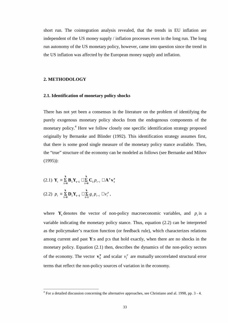
(2.1) yt

yi

k

0iiti

k

0ivAC�YB�Y ++= −=−= itt p

(2.2) ptitit vpgp ++= −=−=

k

1i1ti

k

0i�YD� ,

where tY denotes the vector of non-policy macroeconomic variables, and tp is a

variable indicating the monetary policy stance. Thus, equation (2.2) can be interpreted

as the policymaker’s reaction function (or feedback rule), which characterizes relations

among current and past Y:s and p:s that hold exactly, when there are no shocks in the

monetary policy. Equation (2.1) then, describes the dynamics of the non-policy sectors

of the economy. The vector ytv and scalar y

tv are mutually uncorrelated structural error

terms that reflect the non-policy sources of variation in the economy.

4 For a detailed discussion concerning the alternative approaches, see Christiano and al. 1998, pp. 3 - 4.

34

When it comes to the choice of the monetary policy variable tp , the monetary policy

shock is defined as an unexpected one time change in the short term interest rate under

the central bank’s control. The identification of the monetary policy shocks now

involves making enough identifying assumptions for estimating the parameters of

policymaker’s reaction function. These necessary assumptions involve assumptions

about the variables the monetary authority is interested in when setting the monetary

stance and assumptions about the policymaker’s operating instrument.5 One also must

make an assumption about the way the monetary policy variable (p) and hence the

monetary policy shocks, are related to the variables in the feedback rule.

2.2. Estimation of the monetary policy shocks using SVARs

To ill ustrate the identification of the structural shocks in SVAR modeling, it is

convenient to denote both the policy and non-policy variables of the economy by k-

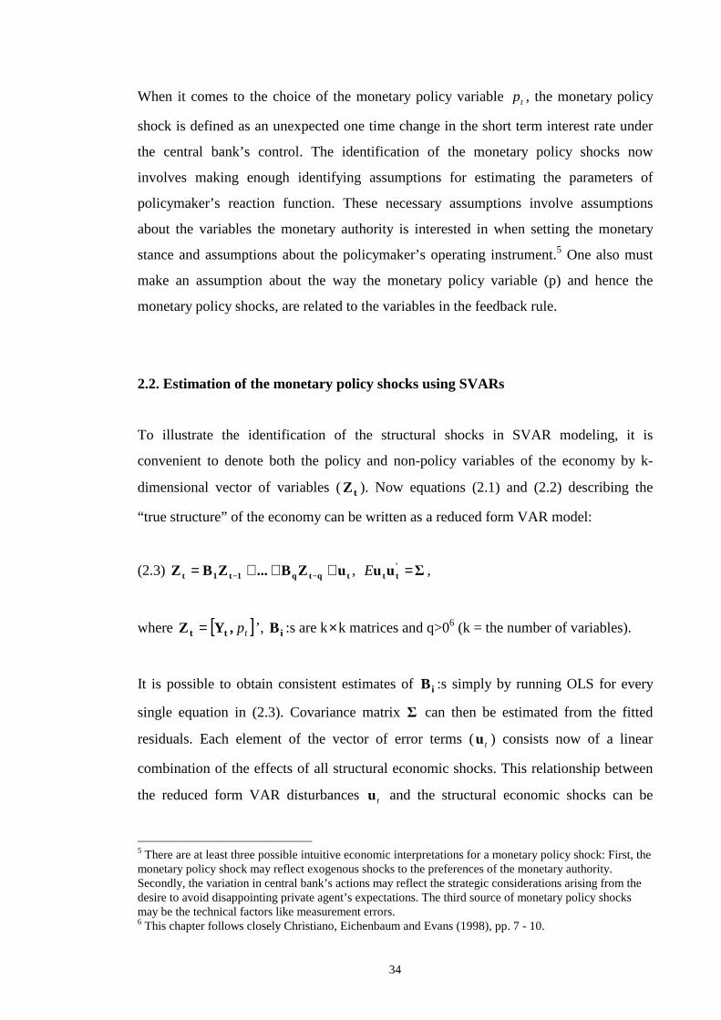
dimensional vector of variables ( tZ ). Now equations (2.1) and (2.2) describing the

“ true structure” of the economy can be written as a reduced form VAR model:

(2.3) ,tqtq1t1t uZB...ZBZ +++= −− �uu 'tt =E ,

where [ ]tp,YZ tt = ’ , iB :s are k×k matrices and q>06 (k = the number of variables).

It is possible to obtain consistent estimates of iB :s simply by running OLS for every

single equation in (2.3). Covariance matrix � can then be estimated from the fitted

residuals. Each element of the vector of error terms ( tu ) consists now of a linear

combination of the effects of all structural economic shocks. This relationship between

the reduced form VAR disturbances tu and the structural economic shocks can be

5 There are at least three possible intuitive economic interpretations for a monetary policy shock: First, the monetary policy shock may reflect exogenous shocks to the preferences of the monetary authority. Secondly, the variation in central bank’s actions may reflect the strategic considerations arising from the desire to avoid disappointing private agent’s expectations. The third source of monetary policy shocks may be the technical factors like measurement errors. 6 This chapter follows closely Christiano, Eichenbaum and Evans (1998), pp. 7 - 10.

35

expressed as tt0 0uA = . 0A is an invertible, square matrix and D00 ,tt =E , where D is

a positively definite matrix.

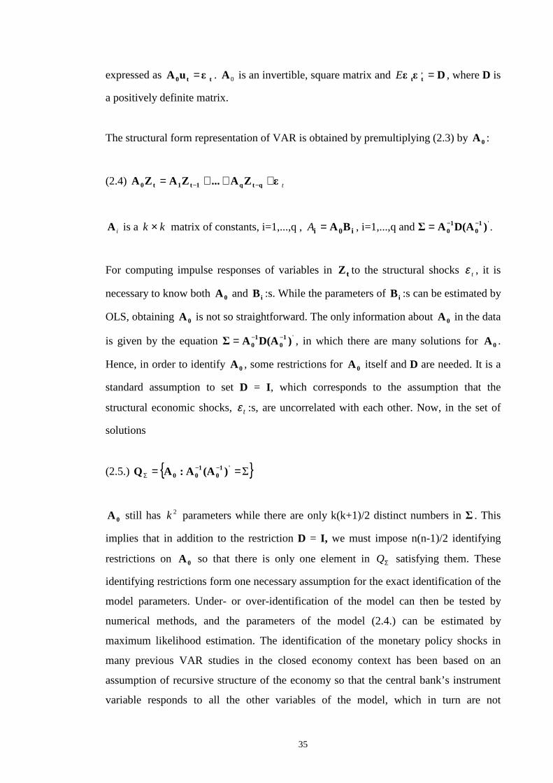
The structural form representation of VAR is obtained by premultiplying (2.3) by 0A :

(2.4) t0ZA...ZAZA qtq1t1t0 +++= −−

iA is a k k× matrix of constants, i=1,...,q , i0i BA=A , i=1,...,q and .')D(AA� 10

10

−−=

For computing impulse responses of variables in tZ to the structural shocks ε t , it is

necessary to know both 0A and iB :s. While the parameters of iB :s can be estimated by

OLS, obtaining 0A is not so straightforward. The only information about 0A in the data

is given by the equation ')D(AA� 10

10

−−= , in which there are many solutions for 0A .

Hence, in order to identify 0A , some restrictions for 0A itself and D are needed. It is a

standard assumption to set D = I , which corresponds to the assumption that the

structural economic shocks, tε :s, are uncorrelated with each other. Now, in the set of

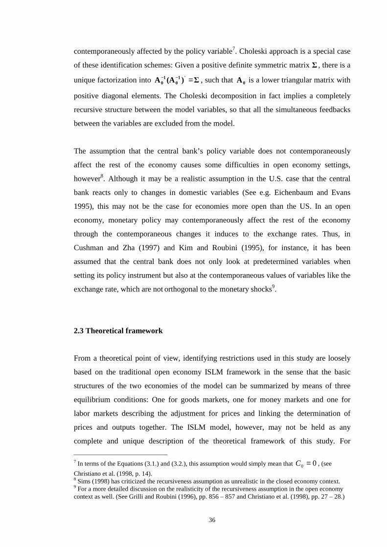
solutions

(2.5.) { }�== −−Σ

'10

100 )(AA:AQ

0A still has k 2 parameters while there are only k(k+1)/2 distinct numbers in � . This

implies that in addition to the restriction D = I , we must impose n(n-1)/2 identifying

restrictions on 0A so that there is only one element in ΣQ satisfying them. These

identifying restrictions form one necessary assumption for the exact identification of the

model parameters. Under- or over-identification of the model can then be tested by

numerical methods, and the parameters of the model (2.4.) can be estimated by

maximum likelihood estimation. The identification of the monetary policy shocks in

many previous VAR studies in the closed economy context has been based on an

assumption of recursive structure of the economy so that the central bank’s instrument

variable responds to all the other variables of the model, which in turn are not

36

contemporaneously affected by the policy variable7. Choleski approach is a special case

of these identification schemes: Given a positive definite symmetric matrix � , there is a

unique factorization into �)(AA '10

10 =−− , such that 0A is a lower triangular matrix with

positive diagonal elements. The Choleski decomposition in fact implies a completely

recursive structure between the model variables, so that all the simultaneous feedbacks

between the variables are excluded from the model.

The assumption that the central bank’s policy variable does not contemporaneously

affect the rest of the economy causes some diff iculties in open economy settings,

however8. Although it may be a realistic assumption in the U.S. case that the central

bank reacts only to changes in domestic variables (See e.g. Eichenbaum and Evans

1995), this may not be the case for economies more open than the US. In an open

economy, monetary policy may contemporaneously affect the rest of the economy

through the contemporaneous changes it induces to the exchange rates. Thus, in

Cushman and Zha (1997) and Kim and Roubini (1995), for instance, it has been

assumed that the central bank does not only look at predetermined variables when

setting its policy instrument but also at the contemporaneous values of variables like the

exchange rate, which are not orthogonal to the monetary shocks9.

2.3 Theoretical framework

From a theoretical point of view, identifying restrictions used in this study are loosely

based on the traditional open economy ISLM framework in the sense that the basic

structures of the two economies of the model can be summarized by means of three

equili brium conditions: One for goods markets, one for money markets and one for

labor markets describing the adjustment for prices and linking the determination of

prices and outputs together. The ISLM model, however, may not be held as any

complete and unique description of the theoretical framework of this study. For

7 In terms of the Equations (3.1.) and (3.2.), this assumption would simply mean that 00 =C , (see

Christiano et al. (1998, p. 14). 8 Sims (1998) has criticized the recursiveness assumption as unrealistic in the closed economy context. 9 For a more detailed discussion on the realisticity of the recursiveness assumption in the open economy context as well . (See Grilli and Roubini (1996), pp. 856 – 857 and Christiano et al. (1998), pp. 27 – 28.)

37

example, it is assumed that the commodity prices and outputs are fixed relative to the

immediate effects of the monetary policy shocks in one period horizon. The ISLM type

models have lately been criti cized fiercely as lacking solid microeconomic foundations.

The empirical relevance of the ISLM model has been studied by Gali (1992) who,

however finds support for the empirical relevance of the ISLM-Philli ps curve paradigm

as a descriptive tool at least for the postwar US-data. Rapach (1998) and Monticelli and

Tristani (1999) provide other two examples of previous studies with an ISLM type

theoretical framework behind the specification of a VAR model.

The variable set of the model consists of the outputs, inflation rates, short and long-term

interest rates and the money supplies of the two countries, along with the nominal

USD/DEM exchange rate. The restrictions imposed on the coeff icient matrix 0A are

represented in Table 2.1 in the next page. The unrestricted parameters are denoted by

1’s, while the 0’s refer to the zero restrictions. The restrictions were selected after

testing several slightly differing alternative sets of restrictions. The differences between

these alternative structuralizations were mainly related to the specification of the

“sluggish sectors” of the economies. Thus, the reaction functions, the money demand

equations as well as the exchange rate equation do not considerably change between the

specifications.10

The final choice between the alternative sets of identification restrictions was based on

the informal criterion for plausibilit y and reasonableness of the impulse responses. This

criterion does not differ in any significant way from what has commonly been done in

empirical research in economics: The model is adjusted until it both fits the data and

gives reasonable results and is thus theoretically acceptable.11 Hence, if the estimation

seemed to yield results that are overall unamenable to any economic interpretation, this

was considered as a sign of misspecification of the given structuralization.

The previous VAR literature has become familiar with a set of puzzling impulse

responses, obviously resulting from specification errors in identifying the monetary

10 The money demand equations were estimated both with and without the long term interest rates. The problem whether to include the foreign output in the reaction functions was also solved by comparing both specifications.

38

policy shocks. These specification errors in turn, can be explained by the diff iculties in

extracting all the other significant determinants of the selected monetary policy variable

from the pure policy effects.

Perhaps the best known of these previous anomalious findings is the so called price

puzzle, in which an expansionary monetary shock is associated with strong and

persistent decline in the price level12. Price puzzle may be interpreted as reflecting the

impacts of the increased inflation expectations, which result in the tightening of the

systematic part of the monetary policy. If the information set of the estimated reaction

function does not capture these expectations, a part of endogenous part of the monetary

policy will be misinterpreted as representing a shock to the policy.

Including the nominal exchange rate among the variables in VAR has given rise to two

additional puzzles, namely the exchange rate and forward discount bias puzzles. The

exchange rate puzzle refers to the empirical findings, according to which the currencies

of some G6 countries have temporarily depreciated against the US dollar after a

monetary contraction. In the case of the forward discount bias in turn, a monetary

contraction has first induced a positive interest rate differential, which is then associated

with a persistent appreciation of the domestic currency. This appreciation, in turn,

implies a failure of the uncovered interest parity condition.13

2.4 The identification restr ictions

To avoid the under-identification problem, the number of the zero restrictions should be

at least (n * (n-1)) / 2, where n is the number of variables in the model. Because the final

model actually includes 56 instead of 55 zero restrictions, it’s exact identifiabilit y had to

be checked by numerical methods (see Appendix IV). According to the results, the

model seems to be exactly identified.

11 See e.g. Leeper and al. (1996) pp. 3 – 5. 12 See e.g. Litterman and Weiss (1985) and Sims (1986) 13 See e.g. Eichenbaum and Evans (1995) and Grilli and Roubini (1996)

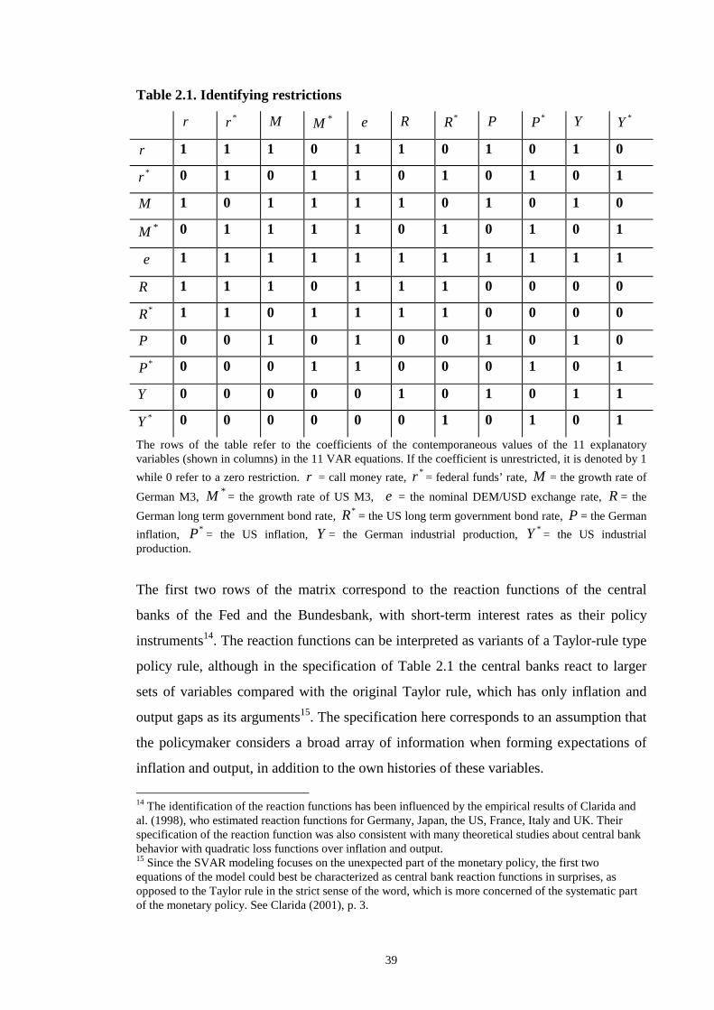
39

Table 2.1. Identifying restr ictions

r *r M *M e R *R P *P Y *Y

r 1 1 1 0 1 1 0 1 0 1 0

*r 0 1 0 1 1 0 1 0 1 0 1

M 1 0 1 1 1 1 0 1 0 1 0

*M 0 1 1 1 1 0 1 0 1 0 1

e 1 1 1 1 1 1 1 1 1 1 1

R 1 1 1 0 1 1 1 0 0 0 0

*R 1 1 0 1 1 1 1 0 0 0 0

P 0 0 1 0 1 0 0 1 0 1 0

*P 0 0 0 1 1 0 0 0 1 0 1

Y 0 0 0 0 0 1 0 1 0 1 1

*Y 0 0 0 0 0 0 1 0 1 0 1

The rows of the table refer to the coeff icients of the contemporaneous values of the 11 explanatory variables (shown in columns) in the 11 VAR equations. If the coeff icient is unrestricted, it is denoted by 1

while 0 refer to a zero restriction. r = call money rate, *r = federal funds’ rate, M = the growth rate of

German M3, *M = the growth rate of US M3, e = the nominal DEM/USD exchange rate, R = the

German long term government bond rate, *R = the US long term government bond rate, P = the German

inflation, *P = the US inflation, Y = the German industrial production, *Y = the US industrial production.

The first two rows of the matrix correspond to the reaction functions of the central

banks of the Fed and the Bundesbank, with short-term interest rates as their policy

instruments14. The reaction functions can be interpreted as variants of a Taylor-rule type

policy rule, although in the specification of Table 2.1 the central banks react to larger

sets of variables compared with the original Taylor rule, which has only inflation and

output gaps as its arguments15. The specification here corresponds to an assumption that

the policymaker considers a broad array of information when forming expectations of

inflation and output, in addition to the own histories of these variables.

14 The identification of the reaction functions has been influenced by the empirical results of Clarida and al. (1998), who estimated reaction functions for Germany, Japan, the US, France, Italy and UK. Their specification of the reaction function was also consistent with many theoretical studies about central bank behavior with quadratic loss functions over inflation and output. 15 Since the SVAR modeling focuses on the unexpected part of the monetary policy, the first two equations of the model could best be characterized as central bank reaction functions in surprises, as opposed to the Taylor rule in the strict sense of the word, which is more concerned of the systematic part of the monetary policy. See Clarida (2001), p. 3.

40

Because the model is estimated with monthly data, the reaction function should only

consist of variables from which there are real-time information available to the central

bank within one month’s time. In practice, the problem boils down to the question

whether to include contemporaneous values of outputs and prices themselves in the

reaction functions or not. According to previous research, it is not clear how much

formal or informal information the monetary authority can collect about the

contemporaneous values of those variables16. Partly motivated by the need to avoid too

large a number of zero restrictions, the contemporaneous values of the domestic output

and inflation are, however, included in the reaction functions.17

The money stock, long-term interest rate, output and inflation of the respective foreign

country are omitted from the reaction functions of both central banks simply because

these variables are assumed not to be of interest to the policymakers. The specifications

of the reaction functions differ from each other in that the Bundesbank is expected also

to look at the foreign short-term interest rate while the Federal Reserve is not. The

domestic long-term interest rates are included to the reaction functions because the long

rates may reflect information about expected inflation.

The third and the fourth row characterize the money demand equations of the countries.

In both countries the change in demand for nominal money is affected by the

contemporaneous values of output, inflation, foreign money growth, nominal exchange

rate and nominal short and long term interest rates18 of the respective country19. This

specification of money demand is close to the standard specifications where the demand

for real money depends on the short-term nominal interest rate and output. The inclusion

of the foreign money in the money demand equations is theoretically motivated by the

16 According to Eichenbaum (1998) for instance, the assumption that the Federal Reserve looks at the current output and price level when setting the monetary policy stance, seems at least as plausible as assuming that it does not. 17 For a more detailed discussion of the reasonableness of this kind of restrictions for the central banks’ information set, see Sims et al. (1998), p. 25, or Christiano, Eichenbaum and Evans (1998), p. 18. 18 It is assumed in this specification of the money demand that the two alternative assets to the agents are cash and bonds. Hence, the opportunity cost of holding cash balances is the nominal rather than real interest rate. 19 The real balances are implicitly defined in terms of consumer prices. Hence, the coeff icient of the nominal exchange rate is not restricted to zero in the money demand equations.

41

need to take into account the currency substitution and the growth rate of world money

for the money demands of the countries20.

The row describing the determination of the nominal DEM/USD exchange rate (e), is an

“ information market equation” , which contains all the variables contemporaneously.

The motivation behind this kind of specification for the determination of the exchange

rate is based on the idea that in eff icient exchange markets the exchange rate can

respond quickly to all relevant information in both countries. The specification is

inspired by the examples of Cushman and Zha (1997) and Sims (1996) and the equation

reflects the existence of disturbances to the private sectors of the countries that cannot

be defined in terms of the sticky non-financial variables included in the model.

The next two rows describe the determination of the long-term interest rates. The

inclusion of the long-term interest rates as variables to VAR is motivated by three

considerations: Firstly, there are some a priori reasons to believe that for many long-

term consumption and investment decisions, the long-term interest rate should be a

variable of more interest than the short run rate (see e.g. Taylor (1995), p. 17). Secondly,

as has been argued by Grilli and Roubini (1996), the movements in long-term interest

rates might be capturing agents’ expectations about long-term inflationary trends.

Finally, according to the empirical evidence provided by Bagliano and Favero (1998),

the contemporaneous long-term interest rate may be relevant variables in the

policymaker’s reaction function.21 The long-term interest rates of both countries are

assumed to respond contemporaneously to movements in all other interest rate variables

of the model, in the exchange rate and in the money supply growth of the home country.

Just like the nominal exchange rate, the long-term interest rates are assumed to be

determined in the capital markets, reflecting a broad array of information of different

variables affecting the investor’s expectations.

20 For a discussion about the foreign money supply for the monetary autonomies of the US and the ERM countries, see Heimonen 1999, p. 2. For a more general discussion about the international currency substitution, see McKinnon (1982). 21 There is actually one problem in including the long-term interest rate as a variable in the VAR model designed to study monetary transmission which is related to distinguishing the structural shocks to long-term rates from structural shocks to short-term rates. This identification problem is due to the feedbacks between interest rates of the different maturities.

42

Rows 8 –11 constitute the sluggish sectors of the two economies. The variables in this

block are assumed not to respond contemporaneously to monetary innovations, but

instead, to be predetermined relative to the monetary policy shocks.22 According to the

rows 8 and 9, inflation is driven by the contemporaneous domestic output levels,

changes in the growth rates of money and the exchange rate. The last two rows of Table

3.1 refer to the outputs (industrial productions) of both countries ( * and YY ). The

outputs are supposed to be affected contemporaneously by the domestic long term

interest rates and inflation rates. In addition, the German output is supposed to instantly

react to changes in the US output, but not the other way round.

3. REDUCED FORM VAR

3.1. Data

Estimating a SVAR model requires first estimating the VAR model in it’s reduced form.

The reduced form VAR model is estimated using monthly data over the sample period

1974:1 to 1998:10. The sample period starts shortly after the collapse of the Bretton-

Woods system and the beginning of the flexible exchange rate regime between the US

and Germany. The number of observations is 297. The source of the data has mainly

been the IMF financial statistics CD-ROM except for the German M3 monetary

aggregate time series, which was provided by the German Bundesbank. Seasonally

unadjusted data is used whenever it has been available to avoid the loss of information

caused by filtering which may also create some artificial structure to the time series

processes. Exceptions had to be made with the output series that are seasonally adjusted

by IMF. The data set of the model consists of the following series:

22 The specification where the monetary policy variable is assumed not to have any contemporaneous effect on the real sector variables is in accordance with many previous empirical studies (Gali 1992, Sims 1998 etc.) which assume some kind of inertia in the real variables. Sims (1996) provides discussion about the significance of this specification for the identifiabilit y of the VAR model.

43

• Logarithmic levels of industr ial production volume indices of both countries23.

These series are seasonally adjusted because of diff iculties in obtaining seasonally

unadjusted data. The changes of industrial productions reflect changes in GDP

which would have been more natural choice of variable. However, it was not

possible to find monthly data of the GDP.

• Short term nominal interest rates of the countries. The representative German

short rate is the call money rate, while federal funds’ rate represents the US short

rate. Both of these interest rates are ‘day to day rates’ reflecting the borrowing costs

in the interbank lending market. The series are seasonally unadjusted and expressed

on levels.

• Long term nominal interest rates of both countr ies, also on seasonally unadjusted

levels. Both rates are 10-year government bond rates and both the short term and

long term interest rates are expressed as monthly averages.

• Seasonally unadjusted logarithmic differences of the consumer pr ice indices of the

countries.

• Seasonally unadjusted logarithmic differences of M3 monetary aggregate of both

countries.

• The nominal DEM/USD exchange rates on logarithmic levels. The figures are

monthly averages.

The data is represented as line graphs in both levels and differences in Appendix I. It is

known a priori, and it can be seen in the graphs, that some important institutional

changes have taken place during the sample period. The most important possible

structural breaks can be listed as follows:

23 In all of the index numbers used as variables the base year is 1990 (=100).

44

• In the periods 1973 – 1975 and 1978 – 1980, the western economies were hit by two

oil price shocks, which resulted in a sharp rise in both inflation and unemployment.

• At the turn of the 1970’s and the 1980’s, strict monetarist principles were introduced

into US monetary policy, due to an attempt to fight against inflation. In practice, the

regime shift was implemented by changing the operating procedures of the Federal

Reserve from interest rate targeting to the targeting of monetary aggregates. The

years from the late 70’s to mid 80’s were also a period of sharp and steady

appreciation of the US dollar against DEM due to the sharp rise in the US interest

rates.

• The reunification of Germany at the beginning of 1990 made the monetary

management a more complex issue for the Bundesbank. For example, the one for

one currency exchange resulted in a peak of 13% in the German M3 aggregate

within a single month. The response of the Bundesbank to this increase in the money

stock was the aggressive tightening of the monetary stance, which for its part

contributed to the collapse of the EMS system in September 1992.

The graphs of Appendix I show that probably there are deterministic trends in the series

of price levels, industrial productions and money supplies of both countries, as

expected. In addition, a visual inspection of the German M3 graph shows evidence of

seasonal components in the respective data generating process. It is natural also to

expect some seasonality for the US M3 and the outputs and prices of both countries.

There is, however, no need to remove the deterministic trends before estimation of the

VAR model, because in the VAR modeling it is possible to approximate a variable with

a trend with a sum of random walk and a drift24. The possible seasonality in the

variables, if necessary, can be taken into account simply by including seasonal dummies

to the estimable VAR model.

24 When a VAR model with a constant and a deterministic trend contains one or more variables that are random walks with drifts, the estimators of the parameters other than the deterministic trend vector will be consistent. (Starck, 1990, p. 41.)

45

The preliminary data analysis was supplemented by looking at the skewness and

kurtosis of the series, as well as the correlograms (the results not reported). The

variables appeared clearly not to be normally distributed, while skewness seemed to be a

more diff icult problem than kurtosis. The correlograms of the series show peaks in the

first partial autocorrelations while the autocorrelations die away very slowly. The result

may be interpreted as an obvious sign of the existence of unit roots in the processes.

The order of integration of the variables was examined by the ADF-, Phili p-Perron and

KPSS tests. Great caution must be exercised in interpreting these results, on the other

hand, because of the low power of the unit root tests. The results of the unit root tests

are summarized in Table II .1 in Appendix II . All variables except call money appear to

be integrated at least of order one (I(1)) in 1 % significance level according to all of the

tests. For call money, however, neither the null hypotheses of stationarity nor the null of

unit root are rejected. These contradictory results can be interpreted as showing that the

time series has not been long enough to properly capture the long run properties of the

data.

For price levels and M3:s of both countries the ADF tests do not reject I(2):ness at 5%

significance level. In addition, the KPSS test rejects I(1):ness at 5% level for prices of

both countries and US M3. Further, there is also some previous empirical research

which provides some support for specifying these variables as I(2). Juselius (1998)

suggests that inflation follows random walk25 and Gali (1992) and Rapach (1998)

specifies M1:s to be I(2). Thus, the specification of the VAR model was based on the

conclusion of one unit root in all variables except the prices and the M3:s which are

modeled as I(2):s.

In the case of nonstationary variables in the VAR model, there are three alternative ways

to proceed in the analysis. At first, it is possible to estimate a stationary VAR by

differencing the nonstationary series before estimation. The second possibilit y to handle

nonstationarity is simply not to care about it and estimate the model in levels. The OLS

regressions of the equations in the VAR model yield consistent, although ineff icient

25 Juselius (1999) provides a more detailed explanation why the prices should in general be modeled as I(2).

46

estimates of the parameters describing the system’s dynamics even in the case of I(1)

variables (Philli ps and Durlauf 1986, Hamilton 1994, p. 652.), and the primary goal of

VAR analysis is just to investigate the dynamic relationships between variables, not to

yield exact estimates of the model parameters26. Moreover, in the case of cointegrated

system with trends in the variables and with some additional preconditions fulfill ed,

OLS is a superconsistent estimator27. In addition, Sims and al.(1987) have showed, that

the LR test for lag length has the usual asymptotic distribution, when the test concerns

linear restrictions on coeff icients on mean zero stationary regressors. Cointegrated

variables would also make it possible to estimate the model in an error correction

(ECM) form, which is the third way to handle nonstationarity.

The cointegration properties of the model variables were examined both by looking

what economic theory and previous empirical research have to say, and by formal

testing using the Johansen cointegration test. (For the details of the cointegration

analysis, see Appendix II). Summing up the results, the variables seem to be

cointegrated, although the a priori information and the formal testing provided fairly

contradictory results for the exact number of cointegration relations in the data.

The alternative methods to examine the cointegration rank of the variable set produced

rather conflicting results, which might lead to incorrect specification of an ECM model

and make the results diff icult to give a precise economic interpretation. Thus, our

problem of handling the nonstationarity in the data is reduced to a choice whether to

estimate the model in levels or differences. Although the exact number of cointegration

relationship remains unclear, the existence of the cointegration between the variables

implies that estimating the model in difference form would lead to omitting valuable

information about the long run properties of the data, and hence to misspecification of

the model. From the apparent existence of cointegration between the variables it

26 Philli ps (1998), however, has shown that the estimated impulse responses of the unrestricted VAR:s with some unit roots are inconsistent in the long run. Chan et al. (1977), in turn, have shown that if the components of VAR include random walk components and the model is estimated in levels with deterministic trends, low frequency movements in the estimated impulses will be exaggerated and high frequency movements will be attenuated. 27 Superconsistent estimators converge at a rate n instead of the usual n , where n is the sample size.

47

therefore follows that we estimate the VAR in logarithmic levels28 except for the I(2)

variables, which are included to the model as differences.

3.2. Building and testing the reduced form VAR

The lag length of the reduced form VAR model was examined firstly by the LR tests to

detect the possibilit y to sequentially drop out lags from the model, secondly by the AIC,

SBC and HQ information criteria29 and thirdly, by examining the statistical properties of

residuals of the equations. (To save space, the details of the information criteria and the

LR tests are not reported.) The outcomes of the two different methods for testing the lag

length conflicted sharply with each other, however, since the LR tests proposed using

long lag structures, while the information criteria suggest more parsimonious

specifications with two (AIC) or three (SBC and HQ) lags.30

The examination of the residuals also suggests estimating a model with long lag

structure, because the residuals of the equations for the short interest rates tend to show

signs of autocorrelation when short lag structures are used31. The desire to save degrees

of freedom, however, finally led us to adopt a short lag structure of four lags32. With this

lag structure, the stabilit y of the equations and the statistical properties of the residuals

are improved, compared to the alternative of three lags recommended by the information

criteria33.

28 For a proof of the consistency of VAR representation in levels when there are cointegrated variables in the system, see Hamilton (1994), p. 579. 29 Paulsen (1984) has shown that both the SBC and HQ information criteria are weakly consistent in the case of variables with unit roots. AIC, however, has been shown to overestimate the true lag order with positive propabilit y irrespective of the existence of any unit roots. (see also Jansson 1994, pp. 35-36.) 30 Clarida and Gertler (1996) solved the problems in choosing the lag length, due to a large number of parameters relative to the length of sample period, by including only the lags 1,2,3,6,9 and 12 in their model. For comparison, this kind of staggered lag structure was adopted also here. Only the AIC criteria preferred the models with staggered lags to models with full l ag structures of three or four lags, however. 31 The normality of the residuals was examined with the Jarque-Bera statistics and the results showed non-normality in most cases irrespective of the lag structure 32 One reason for rejecting the long lag structures was that the impulse responses estimated with the long lag structure of the lags 1-8 and 12 overall yielded impulse responses that were more diff icult to interpret than those computed from models with more parsimonious lag structures.

48

The diagnostic tests for the VAR(4) residuals are summarized in Table III .1 in the

Appendix III . (The significance levels are in brackets.) Autocorrelation was detected by

the LM(1) and Ljung-Box Q(20) tests. The LM(1) test rejects the null hypothesis of no

autocorrelation only in the cases of industrial productions of the countries (at 5% level).

According to the Q(20) statistics, six of the residual series are, however, autocorrelated,

when the horizon for detecting the autocorrelation is extended beyond one lag. Luckily,

the autocorrelated residuals leave the OLS estimator unbiased, although its eff iciency is

reduced.

The ARCH(1) statistic measures the heteroscedasticity of the residuals which was found

at 1% significance level in the series of short term interest rates and monetary growths

of both countries, the German inflation rate and the US government bond rate. Visual

inspection suggests that the reported heteroscedasticity seems to be due to some outliers

among the observations.

The Jarque-Bera statistics maintains the null hypothesis of normality in the cases of the

US inflation, M3 growth, industrial production and DEM/USD exchange rate. The

residuals of call money, federal funds’ rate, German inflation rate, German money

growth and German production however all appear to be non-normally distributed at the

1% significance level. In addition, the residuals of the government bond rates of the

countries seem to be non-normal at the 5% level. Luckily, again, the non-normality

appeared to be mainly due to kurtosis, which is a less serious problem than skewness,

because the kurtosis leaves the OLS estimator unbiased.

A possible source for the observed non-normality of the residuals is provided by the few

outlier observations in the data. Thus, the model was re-estimated by introducing some

observation specific dummy variables into the model34. The dummies were set on three

periods. The first one was set just at the beginning of the sample period to take into

account the fluctuations in the German short-term interest rate. The regime change in

33 The normality of residuals is not a critical assumption in VAR modeling, because the properties of OLS estimator are not affected by nonnormality. The autocorrelation in error terms leaves the OLS estimator unbiased but reduces its eff iciency.

49

US monetary policy at the turn of the 1970’s and 1980’s was taken into account with a

whole set of dummies. Finally, the unification of Germany was considered in the

modeling with a single observation specific dummy for period 1990:6. The non-

normality of the residuals was reduced in some cases when the dummies were

introduced (results not reported in detail ). Surprisingly, however, the residuals showed

fewer signs of autocorrelation without than with the dummies. Thus, only the dummy

representing the currency exchange of Germany in the period 1990:6 was included into

the final model.

The stabilit y of the model was preliminary examined by the Cusum-tests, while more

formal testing of the VAR residuals was performed by the RESET, Chow and the

Goldfeld–Quandt tests. The line graphs of the Cusum tests are shown in Appendix III . It

is seen that the V-mask representing 5% confidence levels is slightly crossed in the

cases of only call money rate and German industrial production, when overall , most of

the equations seems to be quite stable.

The results of the formal stabilit y tests are presented in Table III .2 in the Appendix III .

The F-statistics of RESET(3) tests show a possibilit y of misspecification at the 5 %

significance level only for the US government bond rate. F-values of Chow tests, in

turn, find signs of a structural break in the cases of German inflation and growth rate of

M3. Chow tests, could not, however, be computed for the DEM/USD exchange rate,

because the computer program reported near singular matrix.

The Goldfeld-Quandt tests for the VAR equations were performed as LR tests which are

used to find the most possible date for the regime switch. It is seen that the regime

switch dates suggested by the Goldfeld-Quandt tests differ from those proposed by

visual inspection of the Cusum-test figures, since now the most likely date of a regime

switch is at the turn of the 1970’s and the 1980’s for most of the variables. For the US

variables these results get a natural explanation for the change that occurred in the

operating procedure of the Federal Reserve at that time. Unfortunately, the large number

34 There are some drawbacks in introducing dummy variables into the model, however, since the outlier observations may include valuable information about the dynamics of the model. Also some degrees of freedom are lost when using the dummies.

50

of parameters in the model prevents us from taking the possible regime switch into

account by estimating separate models for both regimes.

Overall , we see that some signs of misspecifications or instabilit y were found in some of

the equations. It has to be noted however that when the coeff icients from different sub-

periods are estimated with very high precision, statistically significant differences are

easily found, although the differences are necessarily not large enough to also imply

economically significant differences between the periods. Further, the changes in the

coeff icients of a dynamic model with large number of parameters may offset each other,

thus leaving many important dynamic relationships unaffected.35

4. EFFECTS OF THE US MONETARY POLICY SHOCK

4.1 VMA representation and impulse responses

After the reduced form VAR has now been estimated and plausible set of identifying

restrictions found, it is possible to calculate the impulse responses for the system.

Estimating the impulse response function of a given VAR system is based on deriving

first the vector moving average (VMA) representation of the model, which can be

written in the form

(4.1) tt C(L)Z 0= , where t0 is a vector of structural disturbances.

The relation between the VMA and the structural VAR representation can be seen by

writing the reduced form VAR from Equation (3.3.) as tt vB(L)Z = , and the structural

form VAR (3.4) as tt 0A(L)Z = , where B(L)AA(L) 0= and t0t vA0 = .

35 See Starck (1990), pp. 73 - 74

51

Now it is seen that the structural form VAR is equivalent with the VMA representation

when 1A(L)C(L) −= . The 11*11 elements in the matrix C(L) are lag polynomials,

which represent the impact of j:th structural shock to the i:th variable.

Because of computational diff iculties, the impulse responses are presented without any

confidence bounds. Thus, the statistical significance of the responses is evaluated on the

basis of the magnitude of the peak responses of the variables, measured in terms of

standard deviations. Overall , the magnitude of the responses seems to be quite modest.

The robustness of the impulse-response estimates with respect to the selected pattern for

the identifying restrictions seemed to vary across the variables. The responses of

industrial productions, government bond rates and exchange rates seemed to be more

robust than the responses of short-term interest rates, inflation rates and monetary

growth rates36.

In some cases (e.g. the effect of the US monetary policy to the German short interest

rate and the effects of the German shock to the inflation rates of both countries) the

impulse responses still seemed somewhat implausible and diff icult to give a reasonable

economic interpretation. One possible explanation for these findings may be provided

by the observed signs of kurtosis, autocorrelation and heteroschedasticity in the VAR

residuals that were not possible to remove even by adding observation specific dummy

variables into the model. Although the skewness, autocorrelation and hetero-

schedasticity leave the estimates unbiased, the reduced eff iciency of the estimates may

have caused some spurious regression between the model variables.

36 It is unfortunately not possible to report all the hundreds of estimated impulse-response pictures.

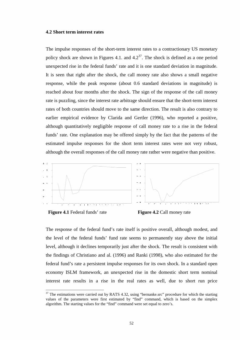
52

4.2 Short term interest rates

The impulse responses of the short-term interest rates to a contractionary US monetary

policy shock are shown in Figures 4.1. and 4.237. The shock is defined as a one period

unexpected rise in the federal funds’ rate and it is one standard deviation in magnitude.

It is seen that right after the shock, the call money rate also shows a small negative

response, while the peak response (about 0.6 standard deviations in magnitude) is

reached about four months after the shock. The sign of the response of the call money

rate is puzzling, since the interest rate arbitrage should ensure that the short-term interest

rates of both countries should move to the same direction. The result is also contrary to

earlier empirical evidence by Clarida and Gertler (1996), who reported a positive,

although quantitatively negligible response of call money rate to a rise in the federal

funds’ rate. One explanation may be offered simply by the fact that the patterns of the

estimated impulse responses for the short term interest rates were not very robust,

although the overall responses of the call money rate rather were negative than positive.

Figure 4.1 Federal funds’ rate Figure 4.2 Call money rate

The response of the federal fund’s rate itself is positive overall , although modest, and

the level of the federal funds’ f und rate seems to permanently stay above the initial

level, although it declines temporarily just after the shock. The result is consistent with

the findings of Christiano and al. (1996) and Ranki (1998), who also estimated for the

federal fund’s rate a persistent impulse responses for its own shock. In a standard open

economy ISLM framework, an unexpected rise in the domestic short term nominal

interest rate results in a rise in the real rates as well , due to short run price

37 The estimations were carried out by RATS 4.32, using “bernanke.src” procedure for which the starting values of the parameters were first estimated by “ find” command, which is based on the simplex algorithm. The starting values for the “ find” command were set equal to zero’s.

� � � � � � � � � � � � � � � � ���

�� �

�� �

�� �

�� �

�� �

�� �

� � � � � � � � � � � � � � � � � � ��� !

"# $%

"# $&

'( )*

'( )+

'( ),

'( )(

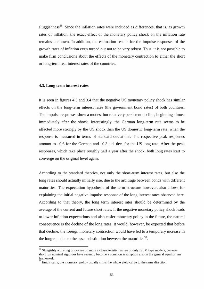
53

sluggishness38. Since the inflation rates were included as differences, that is, as growth

rates of inflation, the exact effect of the monetary policy shock on the inflation rate

remains unknown. In addition, the estimation results for the impulse responses of the

growth rates of inflation even turned out not to be very robust. Thus, it is not possible to

make firm conclusions about the effects of the monetary contraction to either the short

or long-term real interest rates of the countries.

4.3. Long term interest rates

It is seen in figures 4.3 and 3.4 that the negative US monetary policy shock has similar

effects on the long-term interest rates (the government bond rates) of both countries.

The impulse responses show a modest but relatively persistent decline, beginning almost

immediately after the shock. Interestingly, the German long-term rate seems to be

affected more strongly by the US shock than the US domestic long-term rate, when the

response is measured in terms of standard deviations. The respective peak responses

amount to –0.6 for the German and –0.3 std. dev. for the US long rate. After the peak

responses, which take place roughly half a year after the shock, both long rates start to

converge on the original level again.

According to the standard theories, not only the short-term interest rates, but also the

long rates should actually initially rise, due to the arbitrage between bonds with different

maturities. The expectation hypothesis of the term structure however, also allows for

explaining the initial negative impulse response of the long interest rates observed here.

According to that theory, the long term interest rates should be determined by the

average of the current and future short rates. If the negative monetary policy shock leads

to lower inflation expectations and also easier monetary policy in the future, the natural

consequence is the decline of the long rates. It would, however, be expected that before

that decline, the foreign monetary contraction would have led to a temporary increase in

the long rate due to the asset substitution between the maturities39.

38 Sluggishly adjusting prices are no more a characteristic feature of only ISLM type models, because short run nominal rigidities have recently become a common assumption also in the general equili brium framework. 39 Empirically, the monetary policy usually shifts the whole yield curve to the same direction.

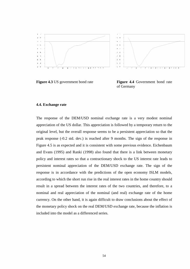
54

Figure 4.3 US government bond rate Figure 4.4 Government bond rate

of Germany

4.4. Exchange rate

The response of the DEM/USD nominal exchange rate is a very modest nominal

appreciation of the US dollar. This appreciation is followed by a temporary return to the

original level, but the overall response seems to be a persistent appreciation so that the

peak response (-0.2 std. dev.) is reached after 9 months. The sign of the response in

Figure 4.5 is as expected and it is consistent with some previous evidence. Eichenbaum

and Evans (1995) and Ranki (1998) also found that there is a link between monetary

policy and interest rates so that a contractionary shock to the US interest rate leads to

persistent nominal appreciation of the DEM/USD exchange rate. The sign of the

response is in accordance with the predictions of the open economy ISLM models,

according to which the short run rise in the real interest rates in the home country should

result in a spread between the interest rates of the two countries, and therefore, to a

nominal and real appreciation of the nominal (and real) exchange rate of the home

currency. On the other hand, it is again diff icult to draw conclusions about the effect of

the monetary policy shock on the real DEM/USD exchange rate, because the inflation is

included into the model as a differenced series.

� � � � � � � � � � � � � � � � ���

�� �

��

�� �

��

�� �

��

�� �

��

�� �

� � � � � � � � � � � � � � � � � � ��� ��

�� �

!" #$

!" #%

&' ()

&' (*

&' (+

&' ('

' (+

' (*

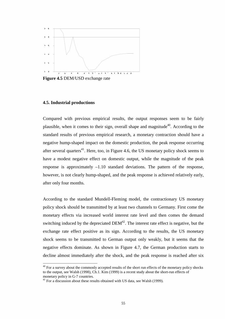
55

Figure 4.5 DEM/USD exchange rate

4.5. Industr ial productions

Compared with previous empirical results, the output responses seem to be fairly

plausible, when it comes to their sign, overall shape and magnitude40. According to the

standard results of previous empirical research, a monetary contraction should have a

negative hump-shaped impact on the domestic production, the peak response occurring

after several quarters41. Here, too, in Figure 4.6, the US monetary policy shock seems to

have a modest negative effect on domestic output, while the magnitude of the peak

response is approximately –1.10 standard deviations. The pattern of the response,

however, is not clearly hump-shaped, and the peak response is achieved relatively early,

after only four months.

According to the standard Mundell -Fleming model, the contractionary US monetary

policy shock should be transmitted by at least two channels to Germany. First come the

monetary effects via increased world interest rate level and then comes the demand

switching induced by the depreciated DEM42. The interest rate effect is negative, but the

exchange rate effect positive as its sign. According to the results, the US monetary

shock seems to be transmitted to German output only weakly, but it seems that the

negative effects dominate. As shown in Figure 4.7, the German production starts to

decline almost immediately after the shock, and the peak response is reached after six

40 For a survey about the commonly accepted results of the short run effects of the monetary policy shocks to the output, see Walsh (1998), Ch.1. Kim (1999) is a recent study about the short-run effects of monetary policy in G-7 countries. 41 For a discussion about these results obtained with US data, see Walsh (1999).

� � � � � � � � � � � � � � � � ���

�� �

�� �

�� �

�� �

�� �

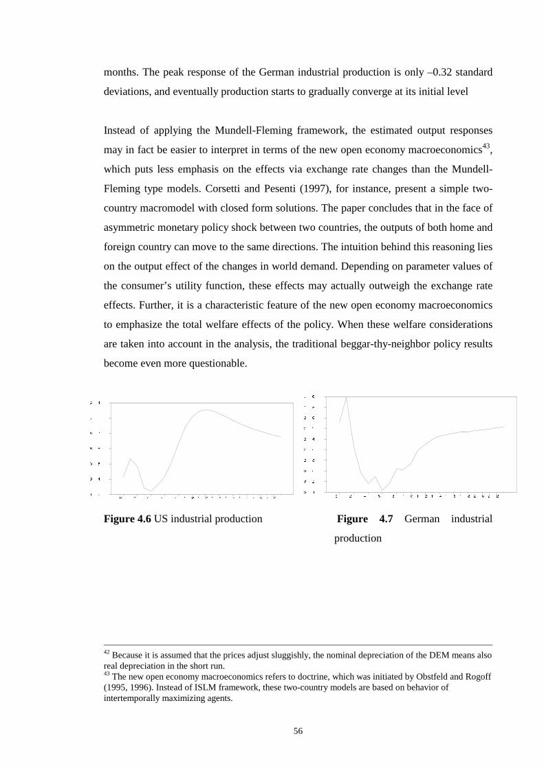
56

months. The peak response of the German industrial production is only –0.32 standard

deviations, and eventually production starts to gradually converge at its initial level

Instead of applying the Mundell -Fleming framework, the estimated output responses

may in fact be easier to interpret in terms of the new open economy macroeconomics43,

which puts less emphasis on the effects via exchange rate changes than the Mundell -

Fleming type models. Corsetti and Pesenti (1997), for instance, present a simple two-

country macromodel with closed form solutions. The paper concludes that in the face of

asymmetric monetary policy shock between two countries, the outputs of both home and

foreign country can move to the same directions. The intuition behind this reasoning lies

on the output effect of the changes in world demand. Depending on parameter values of

the consumer’s utilit y function, these effects may actually outweigh the exchange rate

effects. Further, it is a characteristic feature of the new open economy macroeconomics

to emphasize the total welfare effects of the policy. When these welfare considerations

are taken into account in the analysis, the traditional beggar-thy-neighbor policy results

become even more questionable.

Figure 4.6 US industrial production Figure 4.7 German industrial

production

42 Because it is assumed that the prices adjust sluggishly, the nominal depreciation of the DEM means also real depreciation in the short run. 43 The new open economy macroeconomics refers to doctrine, which was initiated by Obstfeld and Rogoff (1995, 1996). Instead of ISLM framework, these two-country models are based on behavior of intertemporally maximizing agents.

� � � � � � � � � � � � � � � � � � ��� �

�� �

��

�

� �

� �

�� �

� � � � � � � � � � � � � � � � � � ��� �

�� �

��

�� !

�� "

�� �

�� �

��

�# !

�# "

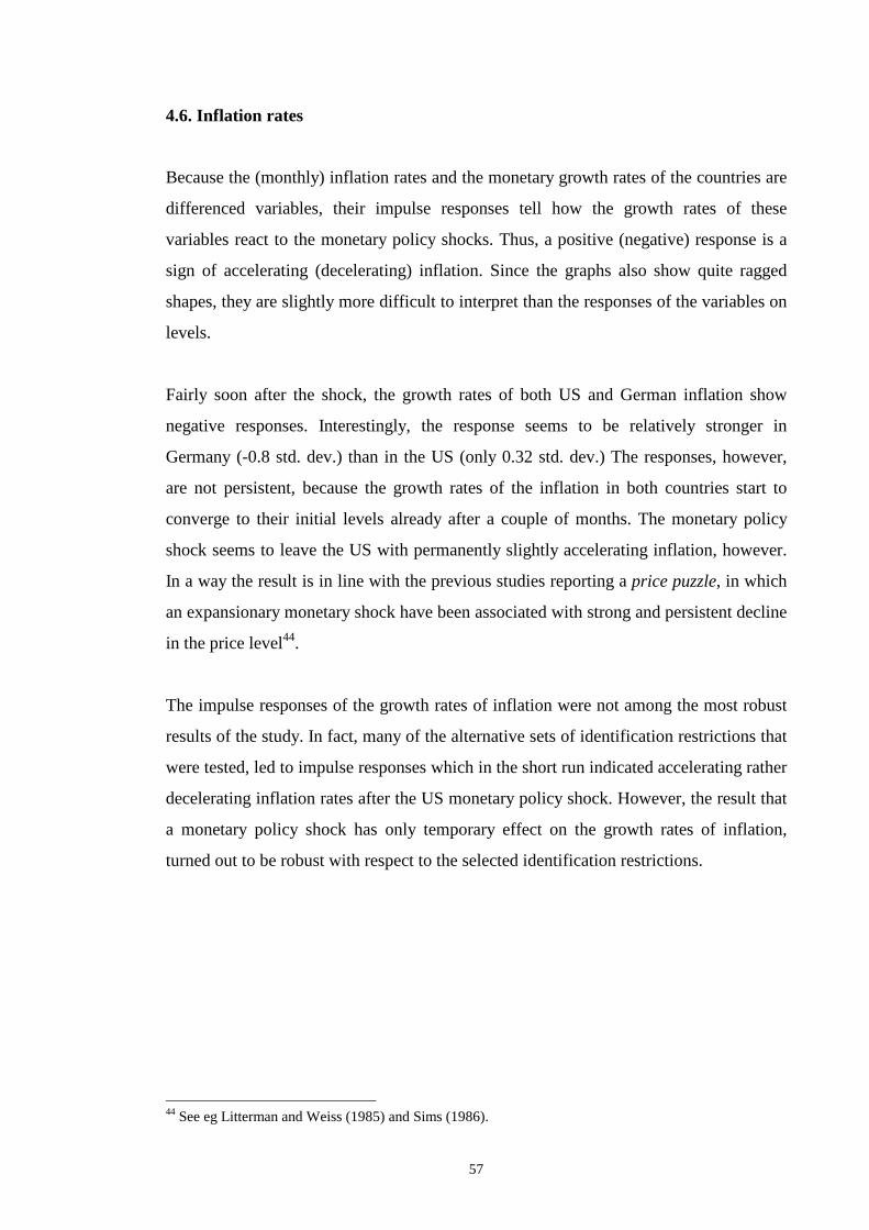
57

4.6. Inflation rates

Because the (monthly) inflation rates and the monetary growth rates of the countries are

differenced variables, their impulse responses tell how the growth rates of these

variables react to the monetary policy shocks. Thus, a positive (negative) response is a

sign of accelerating (decelerating) inflation. Since the graphs also show quite ragged

shapes, they are slightly more diff icult to interpret than the responses of the variables on

levels.

Fairly soon after the shock, the growth rates of both US and German inflation show

negative responses. Interestingly, the response seems to be relatively stronger in

Germany (-0.8 std. dev.) than in the US (only 0.32 std. dev.) The responses, however,

are not persistent, because the growth rates of the inflation in both countries start to

converge to their initial levels already after a couple of months. The monetary policy

shock seems to leave the US with permanently slightly accelerating inflation, however.

In a way the result is in line with the previous studies reporting a price puzzle, in which

an expansionary monetary shock have been associated with strong and persistent decline

in the price level44.

The impulse responses of the growth rates of inflation were not among the most robust

results of the study. In fact, many of the alternative sets of identification restrictions that

were tested, led to impulse responses which in the short run indicated accelerating rather

decelerating inflation rates after the US monetary policy shock. However, the result that

a monetary policy shock has only temporary effect on the growth rates of inflation,

turned out to be robust with respect to the selected identification restrictions.

44 See eg Litterman and Weiss (1985) and Sims (1986).

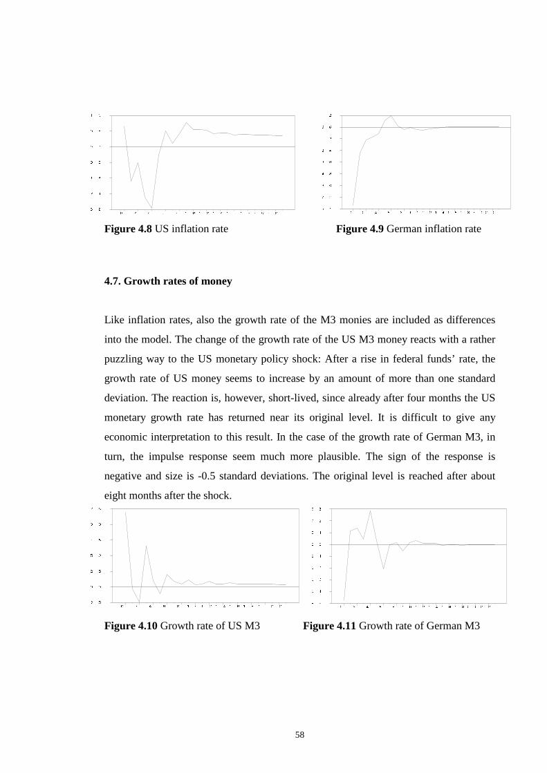
58

Figure 4.8 US inflation rate Figure 4.9 German inflation rate

4.7. Growth rates of money

Like inflation rates, also the growth rate of the M3 monies are included as differences

into the model. The change of the growth rate of the US M3 money reacts with a rather

puzzling way to the US monetary policy shock: After a rise in federal funds’ rate, the

growth rate of US money seems to increase by an amount of more than one standard

deviation. The reaction is, however, short-li ved, since already after four months the US

monetary growth rate has returned near its original level. It is diff icult to give any

economic interpretation to this result. In the case of the growth rate of German M3, in

turn, the impulse response seem much more plausible. The sign of the response is

negative and size is -0.5 standard deviations. The original level is reached after about

eight months after the shock.

Figure 4.10 Growth rate of US M3 Figure 4.11 Growth rate of German M3

� � � � � � � � � � � � � � � � ���

� �

�� �

�� �

�� �

�� �

�� �

� � � � � � � � � � � � � � � � � � ��� �

�� �

�� �

�� �

�� �

�� �

�� �

�� �

�� �

� � � � ! � ! � ! � ! � ! � � � �"� #

"� �

"� #

"# �

$% &

$' '

$( &

) * + , - . ) . * . + . , . - * ) * */) 01

/) 0+

/) 02

/) 0*

/) 0.

/) 0)

) 0.

) 0*

) 02

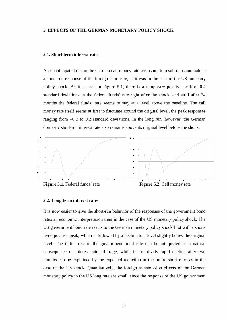
59

5. EFFECTS OF THE GERMAN MONETARY POLICY SHOCK

5.1. Short term interest rates

An unanticipated rise in the German call money rate seems not to result in as anomalous

a short-run response of the foreign short rate, as it was in the case of the US monetary

policy shock. As it is seen in Figure 5.1, there is a temporary positive peak of 0.4

standard deviations in the federal funds’ rate right after the shock, and sitill after 24

months the federal funds’ rate seems to stay at a level above the baseline. The call

money rate itself seems at first to fluctuate around the original level, the peak responses

ranging from –0.2 to 0.2 standard deviations. In the long run, however, the German

domestic short-run interest rate also remains above its original level before the shock.

Figure 5.1. Federal funds’ rate Figure 5.2. Call money rate 5.2. Long term interest rates It is now easier to give the short-run behavior of the responses of the government bond

rates an economic interpretation than in the case of the US monetary policy shock. The

US government bond rate reacts to the German monetary policy shock first with a short-

li ved positive peak, which is followed by a decline to a level slightly below the original

level. The initial rise in the government bond rate can be interpreted as a natural

consequence of interest rate arbitrage, while the relatively rapid decline after two

months can be explained by the expected reduction in the future short rates as in the

case of the US shock. Quantitatively, the foreign transmission effects of the German

monetary policy to the US long rate are small , since the response of the US government

� � � � � � � � � � � � � � � � � � ��� ��

�� ��

� ��

� ��

� ��

� ��

� ��

�

�

� � � � � � � � � � � � � � � � � ��� �

�� �

�� �

�� �

�� �

�� �

�� �

� !

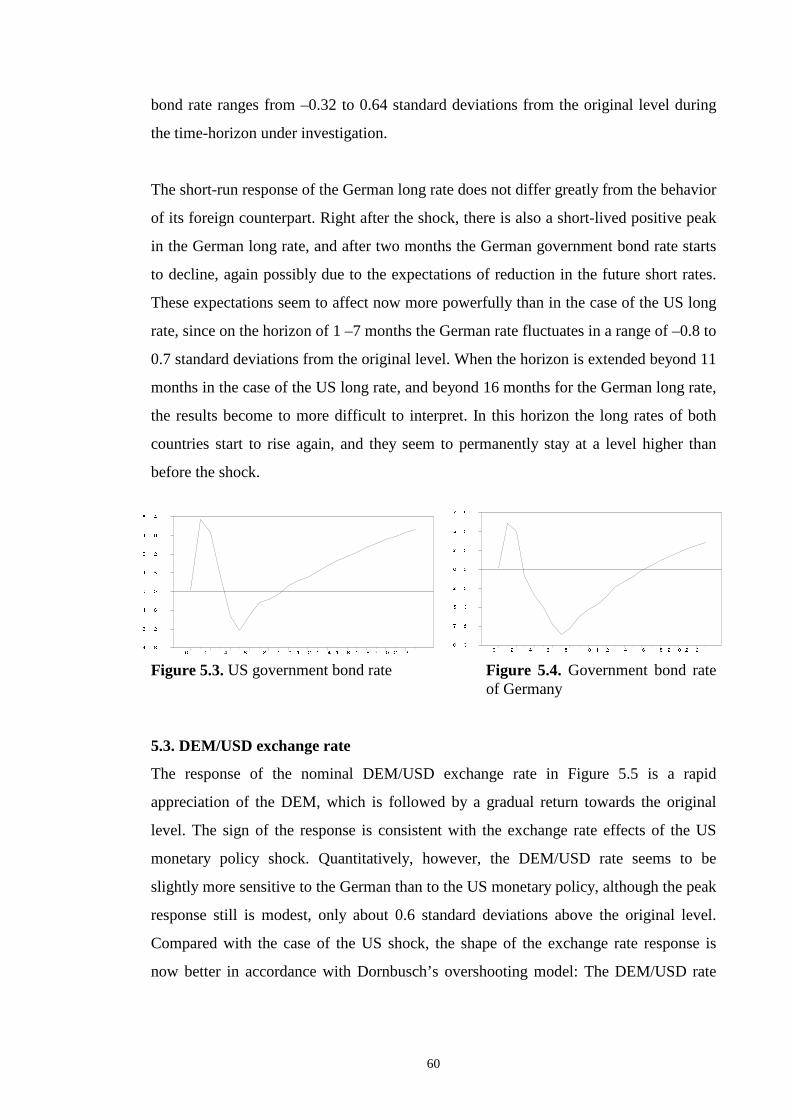
60

bond rate ranges from –0.32 to 0.64 standard deviations from the original level during

the time-horizon under investigation.

The short-run response of the German long rate does not differ greatly from the behavior

of its foreign counterpart. Right after the shock, there is also a short-li ved positive peak

in the German long rate, and after two months the German government bond rate starts

to decline, again possibly due to the expectations of reduction in the future short rates.

These expectations seem to affect now more powerfully than in the case of the US long

rate, since on the horizon of 1 –7 months the German rate fluctuates in a range of –0.8 to

0.7 standard deviations from the original level. When the horizon is extended beyond 11

months in the case of the US long rate, and beyond 16 months for the German long rate,

the results become to more diff icult to interpret. In this horizon the long rates of both

countries start to rise again, and they seem to permanently stay at a level higher than

before the shock.

Figure 5.3. US government bond rate Figure 5.4. Government bond rate of Germany

5.3. DEM/USD exchange rate

The response of the nominal DEM/USD exchange rate in Figure 5.5 is a rapid

appreciation of the DEM, which is followed by a gradual return towards the original

level. The sign of the response is consistent with the exchange rate effects of the US

monetary policy shock. Quantitatively, however, the DEM/USD rate seems to be

slightly more sensitive to the German than to the US monetary policy, although the peak

response still i s modest, only about 0.6 standard deviations above the original level.

Compared with the case of the US shock, the shape of the exchange rate response is

now better in accordance with Dornbusch’s overshooting model: The DEM/USD rate

� � � � � � � � � � � � � � � � � � ��� �

��

� �

�� �

� �

��

� �

��

� � � � � � � � � � � � � � � � � � ��� �

�� �

�� �

� �

�� �

� �

�� �

�� �

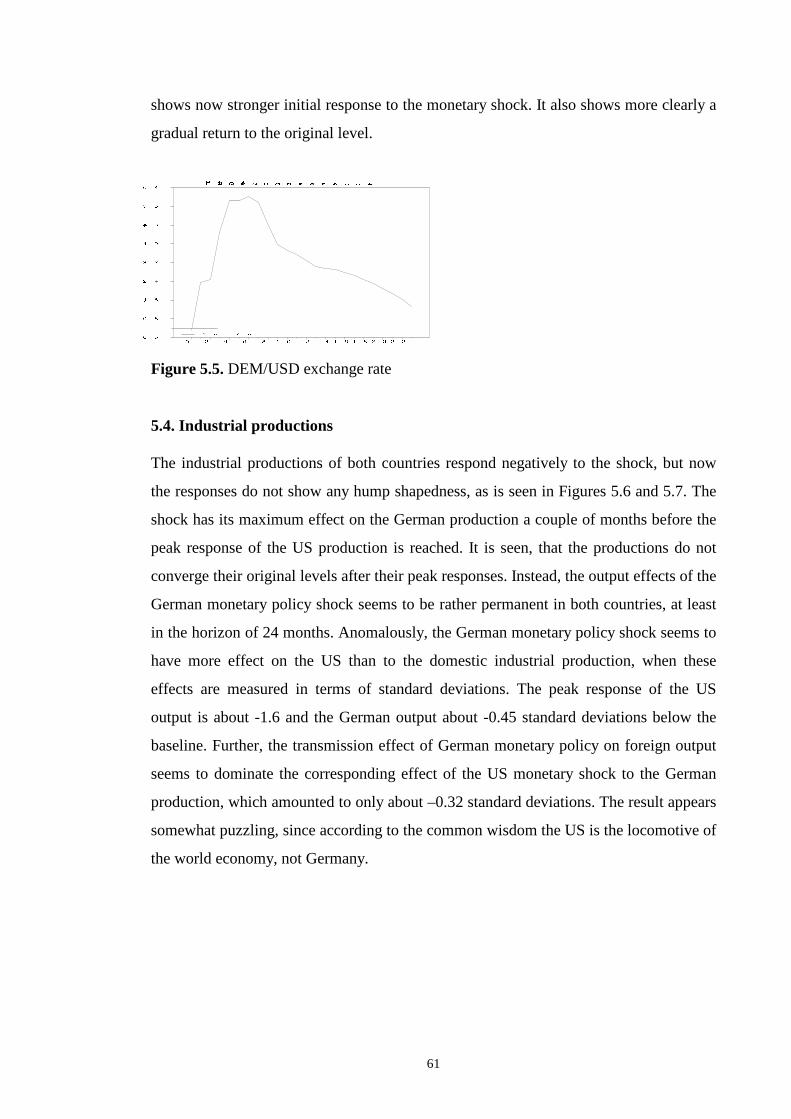
61

shows now stronger initial response to the monetary shock. It also shows more clearly a

gradual return to the original level.

Figure 5.5. DEM/USD exchange rate 5.4. Industr ial productions The industrial productions of both countries respond negatively to the shock, but now

the responses do not show any hump shapedness, as is seen in Figures 5.6 and 5.7. The

shock has its maximum effect on the German production a couple of months before the

peak response of the US production is reached. It is seen, that the productions do not

converge their original levels after their peak responses. Instead, the output effects of the

German monetary policy shock seems to be rather permanent in both countries, at least

in the horizon of 24 months. Anomalously, the German monetary policy shock seems to

have more effect on the US than to the domestic industrial production, when these

effects are measured in terms of standard deviations. The peak response of the US

output is about -1.6 and the German output about -0.45 standard deviations below the

baseline. Further, the transmission effect of German monetary policy on foreign output

seems to dominate the corresponding effect of the US monetary shock to the German

production, which amounted to only about –0.32 standard deviations. The result appears

somewhat puzzling, since according to the common wisdom the US is the locomotive of

the world economy, not Germany.

�� ���� ���� ����� �� � �� � � �� � �� � ���� � � ������

� � � � � � � � � � � � � � � � � ��� �

�� �

�� �

�� �

� !

�" #

�" $

%& '

%' (

)* + , * - )

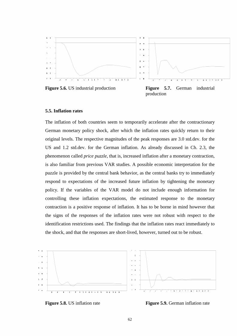
62

Figure 5.6. US industrial production Figure 5.7. German industrial

production 5.5. Inflation rates The inflation of both countries seem to temporarily accelerate after the contractionary

German monetary policy shock, after which the inflation rates quickly return to their

original levels. The respective magnitudes of the peak responses are 3.0 std.dev. for the

US and 1.2 std.dev. for the German inflation. As already discussed in Ch. 2.3, the

phenomenon called price puzzle, that is, increased inflation after a monetary contraction,

is also familiar from previous VAR studies. A possible economic interpretation for the

puzzle is provided by the central bank behavior, as the central banks try to immediately

respond to expectations of the increased future inflation by tightening the monetary

policy. If the variables of the VAR model do not include enough information for

controlli ng these inflation expectations, the estimated response to the monetary

contraction is a positive response of inflation. It has to be borne in mind however that

the signs of the responses of the inflation rates were not robust with respect to the

identification restrictions used. The findings that the inflation rates react immediately to

the shock, and that the responses are short-li ved, however, turned out to be robust.

Figure 5.8. US inflation rate Figure 5.9. German inflation rate

� � � � � � � � � � � � � � � � � � ��� �

�� �

�� �

�� �

�� �

�� �

�� �

�� �

�� �

� � � � � � � � � � � � � � � � � � ��� �

�� �

� �

�� �

�� �

�� �

�� �

�� �

� � � � � � � � � � � � � �� ��

�

��

� �

� ��

� �

� ��

� �

� � � � � � � � � � � � � � � � � � �� !"

� !#

!

!#

!"

!$

!%

& !

& !#

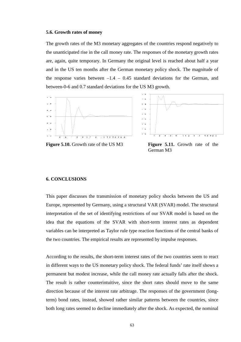
63

5.6. Growth rates of money The growth rates of the M3 monetary aggregates of the countries respond negatively to

the unanticipated rise in the call money rate. The responses of the monetary growth rates

are, again, quite temporary. In Germany the original level is reached about half a year

and in the US ten months after the German monetary policy shock. The magnitude of

the response varies between –1.4 – 0.45 standard deviations for the German, and

between-0-6 and 0.7 standard deviations for the US M3 growth.

Figure 5.10. Growth rate of the US M3 Figure 5.11. Growth rate of the

German M3

6. CONCLUSIONS

This paper discusses the transmission of monetary policy shocks between the US and

Europe, represented by Germany, using a structural VAR (SVAR) model. The structural

interpretation of the set of identifying restrictions of our SVAR model is based on the

idea that the equations of the SVAR with short-term interest rates as dependent

variables can be interpreted as Taylor rule type reaction functions of the central banks of

the two countries. The empirical results are represented by impulse responses.

According to the results, the short-term interest rates of the two countries seem to react

in different ways to the US monetary policy shock. The federal funds’ rate itself shows a

permanent but modest increase, while the call money rate actually falls after the shock.

The result is rather counterintuitive, since the short rates should move to the same

direction because of the interest rate arbitrage. The responses of the government (long-

term) bond rates, instead, showed rather similar patterns between the countries, since

both long rates seemed to decline immediately after the shock. As expected, the nominal

� � � � � � � � � � � � � � � � � � ��� �

��

� �

�

� �

��

�� �

� � � � � � � � � � � � � � � � ��� �

�� �

�� �

�� �

�� �

�� �

�� �

�� �

�� �

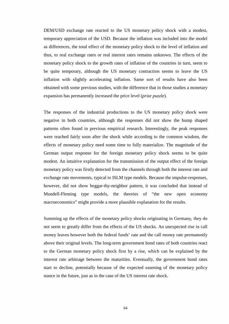
64

DEM/USD exchange rate reacted to the US monetary policy shock with a modest,

temporary appreciation of the USD. Because the inflation was included into the model

as differences, the total effect of the monetary policy shock to the level of inflation and

thus, to real exchange rates or real interest rates remains unknown. The effects of the

monetary policy shock to the growth rates of inflation of the countries in turn, seem to

be quite temporary, although the US monetary contraction seems to leave the US

inflation with slightly accelerating inflation. Same sort of results have also been

obtained with some previous studies, with the difference that in those studies a monetary

expansion has permanently increased the price level (prize puzzle).

The responses of the industrial productions to the US monetary policy shock were

negative in both countries, although the responses did not show the hump shaped

patterns often found in previous empirical research. Interestingly, the peak responses

were reached fairly soon after the shock while according to the common wisdom, the

effects of monetary policy need some time to fully materialize. The magnitude of the

German output response for the foreign monetary policy shock seems to be quite

modest. An intuitive explanation for the transmission of the output effect of the foreign

monetary policy was firstly detected from the channels through both the interest rate and

exchange rate movements, typical to ISLM type models. Because the impulse-responses,

however, did not show beggar-thy-neighbor pattern, it was concluded that instead of

Mundell -Fleming type models, the theories of “ the new open economy

macroeconomics” might provide a more plausible explanation for the results.

Summing up the effects of the monetary policy shocks originating in Germany, they do

not seem to greatly differ from the effects of the US shocks. An unexpected rise in call

money leaves however both the federal funds’ rate and the call money rate permanently

above their original levels. The long-term government bond rates of both countries react

to the German monetary policy shock first by a rise, which can be explained by the

interest rate arbitrage between the maturities. Eventually, the government bond rates

start to decline, potentially because of the expected easening of the monetary policy

stance in the future, just as in the case of the US interest rate shock.

65

As expected, the rise in the call money rate seemed to result in appreciation of the

nominal DEM against the USD. The industrial productions of both countries decline and

remain permanently (in the horizon of 24 months) at a level below the baseline. The

maximum response of the German output is reached already two months after the shock,

while the transmission of the output effect to the US takes a couple of months more time

to fully materialize. It is noteworthy that when measured in terms of standard deviations

the US output seems to react to the German monetary policy shock more strongly than

the other way round. This finding contradicts the commonly accepted view according to

which the US should be the locomotive of the world economy. The variant of price

puzzle discussed above is also faced with the German monetary contraction, since the

German shock seems to permanently accelerate the inflation of both countries.

The robustness of the impulse-response estimates with respect to our identifying

restrictions seemed to vary across the variables. The responses of the industrial

productions, government bond rates and exchange rates seem to be fairly robust, while

the responses of the short-term interest rates, inflation rates and monetary growth rates

are more sensitive to the identifying restrictions used. The sample period considered

include some possible structural breaks in the data generating process, particularly at the

turn of 1970’s to 1980’s, which may have caused some instabilit y in the estimated

SVAR model.

At the end of the paper, we propose some ideas for the future analysis in the field of our

research problem. First, trying to estimate a more parsimonious model with a smaller

number of variables could make the estimated impulse responses less sensitive to the

identification used. The second opportunity to extend the analysis would be linking the

analysis more closely to economic theory, and possibly this way to provide empirical

findings with economic interpretations that are based on more solid microeconomic

foundations.

66

REFERENCES

Bagliano, F. C. – Favero, C. A. (1998) Measur ing monetary policy with VAR models: An evaluation. European Economic Review 42, 1069-1112 Bernanke, B. S. – Blinder, A. (1992) The Federal Fund’s Rate and the Channels of Monetary Transmission American Economic Review 82 (September), 901 – 21. Bernanke, B. S. – Mihov, I. (1995) Measur ing Monetary Policy NBER Workin Paper No. 5145. Chan, K.H. – Hayya, J. C. – Ord, J.K. (1977) A Note on Trend Removal Methods: The Case of Polynomial Regressions versus Var iate Differencing. Econometrica, 45. Christiano, L. J. - Eichenbaum, M. - Evans, C. L. (1998) Monetary Policy Shocks: What have we learned and to what end? NBER Working Paper 6400. Cambridge. Clarida, R. H. (2001)

The Empir ics of Monetary Policy Rules in Open Economies

NBER Working Paper 8603.

Clarida, R. – Gertler, M. (1996) How the Bundesbank Conducts Monetary Policy NBER Working Paper 5581. Cooley, T. F. – Dwyer, M. (1998) Business cycle analysis without much theory. A look at structural VARs. Journal of Econometrics 83 (1998) 57 – 88. Corsetti, G. – Pesenti, P. (1997) Welfare and macroeconomic interdependence Manuscript, Yale University and Princeton University Cushman, D. O. - Tao Zha (1997) Identifying monetary policy in a small open economy under flexible exchange rates. Journal of Monetary Economics, Vol. 39, 433 - 448. Eichenbaum, M. - Evans, C. I. (1995) Some empir ical evidence on the effects of shocks to monetary policy on exchange rates. Quarterly Journal of Economics, 975 - 1009.

67

Gali , J. (1992) How well does the IS-LM model fit postwar U.S. data? Quartely Journal of Economics, Vol. 107, 709 - 738. Gaspar, V. – Issing, O. (2002) Exchange Rates and Monetary Policy Australian Economic Papers 41:4, December. Giannini, C. (1992) Topics in Structural VAR Econometr ics. Springer Verlag. Grilli , V. – Roubini, N. (1996) Liquidity models in open economies: Theory and empir ical evidence. European Economic Review 40, 847-859. Hamilton, J. D. (1994) Time Series Analysis Princeton University Press. Princeton, New Yersey. Hansen, J. D. – Nielsen, J. U.-M. (1997) An Economic Analysis of the EU McGraw-Hill . London. Heimonen, K. (1999) Interaction between US and EU Monetary Policy University of Jyväskylä, Working Paper 194. Jansson, P. (1994) Essays on Empir ical Macroeconomics Department of Economics. Uppsala University. Juselius, K. (1998) A Structural VAR for Denmark Under Changing Monetary Regimes Journal of Business and Economic Statistics, October 1998, Vol. 16, No 4. Juselius, K. (1999) Models and relations in economics and econometr ics Journal of Economic Methodology 6:2. 1999. Kim, S. (1999) Do monetary policy shocks matter in the G-7 countr ies? Using common identifying assumptions about monetary policy across countr ies. Journal of International Economics 48 (1999). Kim, S. – Roubini, N. (1995) Liquidity and Exchange Rates, A Structural VAR Approach Manuscript, New York University

68

Leeper, E. M. - Sims, C. A. - Zha, T. A. (1996) Does Monetary Policy Generate Recessions? A draft. Christopher Sims’ home page: http://eco-072399b.princeton.edu/yftp/bpea/bpeaf.pdf Litterman, R.B. - Weiss, L. (1985) Money, real interest rates and output: A Reinterpretation of postwar U.S. data. Econometrica 53, 129 - 156. McKinnon, R. I. (1982) Currency Substitution and Instabili ty in the Wor ld Dollar Standard American Economic Review, June 1982, pp. 320-333.

McKinnon, J. G. (1991) Critical Values for Cointegration Tests In "Long-Run Economic Relationships” , edited by Engle and Granger, 1991.

Monticelli , C. – Tristani, O. (1999) What does the single monetary policy do? A SVAR benchmark for the European Central Bank. European Central Bank Working paper series May 1999. Obstfeld, M. – Rogoff , K. (1995) Exchange Rate Dynamix Redux Journal of Politi cal Economy, 103, no. 3 (June): 624-660. Obstfeld, M. – Rogoff , K. (1996) Foundations of International Macroeconomics Cambridge, MA: MIT Press Paulsen, J. (1984) Order Determination of Multivar iate Autoregressive Time Series with Unit Roots Journal of Time Series Analysis, 5. Philli ps, P. C.B. (1998) Impulse response and forecast error var iance asymptotics in nonstationary VARs Journal of Econometrics 83 (1998) 21 – 56. Philli ps, P. C. B. – Durlauf, S. N. (1986) Multiple Time Series Regression with Integrated Processes. Review of Economic Studies, 53. Ranki, S. (1998) Monetary Policy in a Bipolar International Monetary System Bank of Finland Discussion Papers 1/98. Helsinki.

69

Rapach, D. E. (1998) Macro schocks and fluctuations. Journal of Economics and Business, Vol. 50, 23 - 38. Schlagenhauf, D. E. - Wrase, J. M. (1995) Liquidity and real activity in a simple open economy model. Journal of Monetary Economics, Vol. 35, 431 - 461. Sims, C. A. (1986) Are forecasting models usable for policy analysis? Federal Reserve Bank of Minneapolis Quarterly Review, Winter, 2 - 16. Sims, C. A. – Stock, J.H. – Watson, M. W. (1987) Inference in L inear Time Series Models with Some Unit Roots. Hoover Institution working Paper No. E-87-1, Stanford. Sims, Christopher A. and Zha, T. A. (1998) Does Monetary Policy Generate Recessions? Federal Reserve Bank of Atlanta, Working Paper 98-12. Sims, C. A. (1998) Whither ISLM Christopher Sims’ home page: http://www.econ.yale.edu/~sims/pub/mpolicy/. Starck, C. C. (1990) Foreign and Domestic Shocks and Fluctuations in the Finnish Economy 1960 – 1988. Bank of Finland, series B:44. Taylor, J. B. (1995) The Monetary Transmission Mechanism: An Empir ical Framework. Journal of Economic Perspectives, Vol. 9, 11-26. Walsh, C. E. (1999) Monetary Theory and Policy The MIT Press.

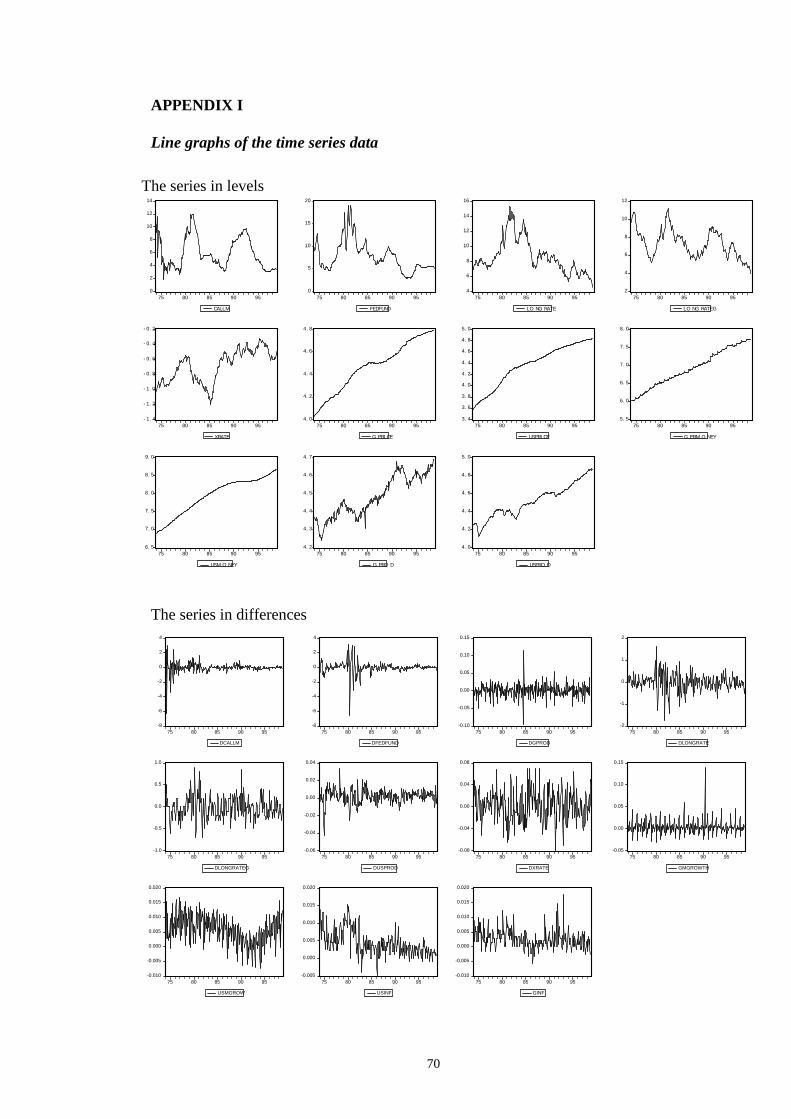
70

APPENDIX I Line graphs of the time series data

The series in levels

The series in differences

-8

-6

-4

-2

0

2

4

75 80 85 90 95

DCALLM

-8

-6

-4

-2

0

2

4

75 80 85 90 95

DFEDFUND

-0.10

-0.05

0.00

0.05

0.10

0.15

75 80 85 90 95

DGPROD

-2

-1

0

1

2

75 80 85 90 95

DLONGRATE

-1.0

-0.5

0.0

0.5

1.0

75 80 85 90 95

DLONGRATEG

-0.06

-0.04

-0.02

0.00

0.02

0.04

75 80 85 90 95

DUSPROD

-0.08

-0.04

0.00

0.04

0.08

75 80 85 90 95

DXRATE

-0.05

0.00

0.05

0.10

0.15

75 80 85 90 95

GMGROWTH

-0.010

-0.005

0.000

0.005

0.010

0.015

0.020

75 80 85 90 95

USMGROW

-0.005

0.000

0.005

0.010

0.015

0.020

75 80 85 90 95

USINF

-0.010

-0.005

0.000

0.005

0.010

0.015

0.020

75 80 85 90 95

GINF

0

2

4

6

8

10

12

14

75 80 85 90 95

CALLM

0

5

10

15

20

75 80 85 90 95

FEDFUND

4

6

8

10

12

14

16

75 80 85 90 95

LO NG RATE

2

4

6

8

10

12

75 80 85 90 95

LO NG RATEG

- 1. 4

- 1. 2

- 1. 0

- 0. 8

- 0. 6

- 0. 4

- 0. 2

75 80 85 90 95

XRATE

4. 0

4. 2

4. 4

4. 6

4. 8

75 80 85 90 95

G PRI CE

3. 4

3. 6

3. 8

4. 0

4. 2

4. 4

4. 6

4. 8

5. 0

75 80 85 90 95

USPRI CE

5. 5

6. 0

6. 5

7. 0

7. 5

8. 0

75 80 85 90 95

G ERM O NEY

6. 5

7. 0

7. 5

8. 0

8. 5

9. 0

75 80 85 90 95

USM O NEY

4. 2

4. 3

4. 4

4. 5

4. 6

4. 7

75 80 85 90 95

G PRO D

4. 0

4. 2

4. 4

4. 6

4. 8

5. 0

75 80 85 90 95

USPRO D

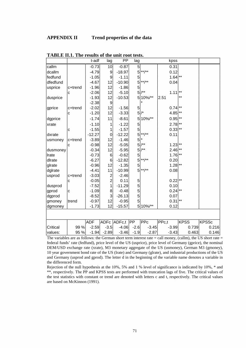
71

APPENDIX II Trend properties of the data

TABLE II .1. The results of the unit root tests. t-adf lag PP lag kpss

callm -0.73 10 -0.87 5 0.31 dcallm -4.79 9 -18.97 5 **/** 0.12 fedfund -1.05 9 -1.11 5 1.64 ** dfedfund -4.67 12 -10.90 5 **/** 0.04 usprice c+trend -1.96 12 -1.86 5

c -2.06 12 -5.10 5 /** 1.11 ** dusprice -1.93 12 -10.53 5 10%/** 2.51 **

-2.38 9 * gprice c+trend -2.02 12 -1.56 5 0.74 **

c -1.20 12 -3.33 5 /* 4.85 ** dgprice -1.74 11 -8.61 5 10%/** 0.95 ** xrate -1.10 1 -1.22 5 2.78 **

c -1.55 1 -1.57 5 0.33 ** dxrate -12.27 0 -12.22 5 **/** 0.11 usmoney c+trend -3.89 12 -1.46 5 *

c -0.98 12 -5.05 5 /** 1.23 ** dusmoney -0.34 12 -5.95 5 /** 2.46 ** lrate -0.73 6 -0.62 5 1.76 ** dlrate -6.27 6 -12.82 5 **/** 0.20 glrate -0.96 12 -1.35 5 1.28 ** dglrate -4.41 11 -10.99 5 **/** 0.08 usprod c+trend -3.03 2 -2.46

c -0.05 2 0.11 5 0.22 ** dusprod -7.52 1 -11.29 5 0.10 gprod c -1.09 8 -0.48 5 0.24 ** dgprod -8.52 3 -26.13 5 0.07 gmoney trend -0.97 12 -0.95 5 0.31 ** dgmoney -1.73 12 -15.57 5 10%/** 0.12

ADF ADFc ADFc,t PP PPc PPc,t KPSS KPSSc

Critical 99 % -2.59 -3.5 -4.06 -2.6 -3.45 -3.99 0.739 0.216 values: 95 % -1.94 -2.89 -3.46 -1.9 -2.87 -3.43 0.463 0.146 The variables are as follows: the German short term interest rate = call money, (callm), the US short rate = federal funds’ rate (fedfund), price level of the US (usprice), price level of Germany (gprice), the nominal DEM/USD exchange rate (xrate), M3 monetary aggregate of the US (usmoney), German M3 (gmoney), 10 year government bond rate of the US (lrate) and Germany (glrate), and industrial productions of the US and Germany (usprod and gprod). The letter d in the beginning of the variable name denotes a variable in the differenced form. Rejection of the null hypothesis at the 10%, 5% and 1 % level of significance is indicated by 10%, * and ** , respectively. The PP and KPSS tests are performed with truncation lags of five. The critical values of the test statistics with constant or trend are denoted with letters c and t, respectively. The critical values are based on McKinnon (1991).

72

The cointegration analysis The analysis of the cointegration properties of the data is started by examining, what economic theory and previous empirical research have to say about the cointegration properties of our VAR system. Following the reasoning of Jacobson et al. (1999)45 we may assume that the nonstationarity in the variables of the VAR model is due to only four independent stochastic trends: Production in both countries is driven by stochastic shocks to domestic technology46 and inflation rates are determined by stochastic shocks to the growth rates of domestic money supply47. Hence, a priori we might expect to find r = 11 – 4 = 7 cointegration relationships in the data. If there are only two stochastic trends among the German variables and other two stochastic trends among the US variables, all the domestic variables of both countries may be cointegrated with each other. According to Juselius (1999 p. 272 - 273), this kind of cointegration relationship between output, real money supply and the spread between the short run and long run interest rates can be interpreted as representing either the money demand equation or the central bank reaction function, depending on the parameter values of the cointegration vector. Two other cointegration relations may be dictated by the term structures of the interest rates, that is, the differences between the short and long term interest rates of both countries48. The fifth and the sixth relations are suggested by the uncovered interest rate parity (UIP) relation which suggests that the interest rate differential between the countries should equal the expected change in the exchange rate. Accordingly, if the exchange rate expectations are I(1), the differential between both short and long term interest rates between the countries should be stationary. The cointegration relation suggested by the purchasing power parity (PPP) condition provides the last possible cointegration relation. The PPP condition relates the inflation differential between the countries to the change in the exchange rate Johansen cointegration test The results of the λ -trace and max−λ tests are summarized in Table III .1. below49. The test were made for variables in levels, except the prices and the growth rates of M3, which are differenced to obtain I(1) series. The series appear to be cointegrated,

45 Jacobson et al. (1999) study the effects of various economic shocks in the small open economy (Sweden) context, estimating an ECM model with seven variables, some of which are from a large foreign economy. 46 Starck (1990) found the outputs of some industrialized countries to be cointegrated after the Bretton Woods era, proposing that the outputs of different countries may be driven by one common, instead of two separate, stochastic trends. 47 Actually, in Jacobson and al. (1999) the prices were assumed to be I(1) variables, whereas here both the price levels and M3:s of the countries are considered to be I(2). With this specification adopted, shocks to the money stock can permanently affect its growth rate as well as the rate of inflation. 48 The stationarity of the interest rate spread is proposed e.g. by Campbell and Schill er (1987). 49 The tables for the critical values for the test statistics are sensitive for including deterministic or dummy variables in the model. Hence, because our model includes a dummy variable, we have computed tables using appropriate option of the CATS computer program, instead of using the standard tables.

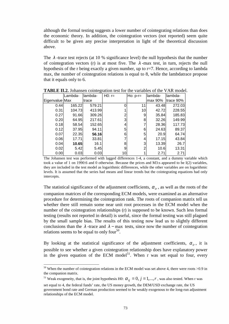
73

although the formal testing suggests a lower number of cointegrating relations than does the economic theory. In addition, the cointegration vectors (not reported) seem quite diff icult to be given any precise interpretation in light of the theoretical discussion above. The λ -trace test rejects (at 10 % significance level) the null hypothesis that the number of cointegration vectors (r) is at most five. The λ -max test, in turn, rejects the null hypothesis of the r being exactly a given number, up to r=7. Hence, according to lambda max, the number of cointegration relations is equal to 8, while the lambdatrace propose that it equals only to 6. TABLE II .2. Johansen cointegration test for the variables of the VAR model.

Lambda- lambda- H0: r= Ho: p-r= lambda- lambda- Eigenvalue Max trace max 90% trace 90%

0.44 165.22 579.21 0 11 43.48 272.03 0.31 104.73 413.99 1 10 42.72 228.55 0.27 91.66 309.26 2 9 35.84 185.83 0.20 64.95 217.61 3 8 32.26 149.99 0.18 58.54 152.65 4 7 28.36 117.73 0.12 37.95 94.11 5 6 24.63 89.37 0.07 22.35 56.16 6 5 20.9 64.74 0.06 17.71 33.81 7 4 17.15 43.84 0.04 10.65 16.1 8 3 13.39 26.7 0.02 5.42 5.45 9 2 10.6 13.31 0.00 0.03 0.03 10 1 2.71 2.71

The Johansen test was performed with lagged differences 1-4, a constant, and a dummy variable which took a value of 1 on 1990:6 and 0 otherwise. Because the prices and M3:s appeared to be I(2) variables, they are included in the test model as logarithmic differences, while the other variables are on logarithmic levels. It is assumed that the series had means and linear trends but the cointegrating equations had only intercepts. The statistical significance of the adjustment coeff icients, irα , as well as the roots of the

companion matrices of the corresponding ECM models, were examined as an alternative procedure for determining the cointegration rank. The roots of companion matrix tell us whether there still remain some near unit root processes in the ECM model when the number of the cointegration relationships (r) is supposed to be known. Such less formal testing (results not reported in detail ) is useful, since the formal testing was still plagued by the small sample bias. The results of this testing now lead us to slightly different conclusions than the λ -trace and max−λ tests, since now the number of cointegration relations seems to be equal to only four50. By looking at the statistical significance of the adjustment coeff icients, irα , it is

possible to see whether a given cointegration relationship does have explanatory power in the given equation of the ECM model51. When r was set equal to four, every

50 When the number of cointegration relations in the ECM model was set above 4, there were roots >0.9 in the companion matrix. 51 Weak exogeneity, that is, the joint hypothesis H0: rjij ,...,1,0 ==α , was also tested. When r was

set equal to 4, the federal funds’ rate, the US money growth, the DEM/USD exchange rate, the US government bond rate and German production seemed to be weakly exogenous to the long-run adjustment relationships of the ECM model.

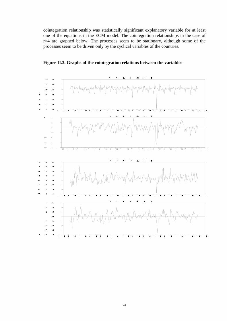
74

cointegration relationship was statistically significant explanatory variable for at least one of the equations in the ECM model. The cointegration relationships in the case of r=4 are graphed below. The processes seem to be stationary, although some of the processes seem to be driven only by the cyclical variables of the countries. Figure II .3. Graphs of the cointegration relations between the var iables

� �� � ��� �� � ������ �� ��

� � �� � � �� � � �� � � �� � � �� � � �� � � � � � �� � � !� � � �� � � �� � � � � � �"# $ $

%& ' (

%& ( (

%' ' (

%' ( (

%) ' (

%) ( (

*+ , -

. /. / 001 21 2 343455 66 708708

9 : ; <9 : ; =9 : ; >9 : > ?9 : > @9 : > <9 : > =9 : > >9 : : ?9 : : @9 : : <9 : : =9 : : >A9 ? ?

A; B

AB ?

A@ B

?

@ B

B ?

; B

C DC D EEF GF G HIHIJJ KK LEMLEM

N O P QR S T UV W X YZ [ \ ]^ _ ` a^ _ ` b^ _ ` c^ _ ` `^ _ _ d^ _ _ a^ _ _ b^ _ _ c^ _ _ `ef g h

ef i h

ef j h

ef h h

ek h

eg h

ei h

l ml m nno po p qrqrss tt unvunv

w x y zw x y {w x y |w x | }w x | ~w x | zw x | {w x | |w x x }w x x ~w x x zw x x {w x x |�~ }

�� �

�� �

��

�

�

� �

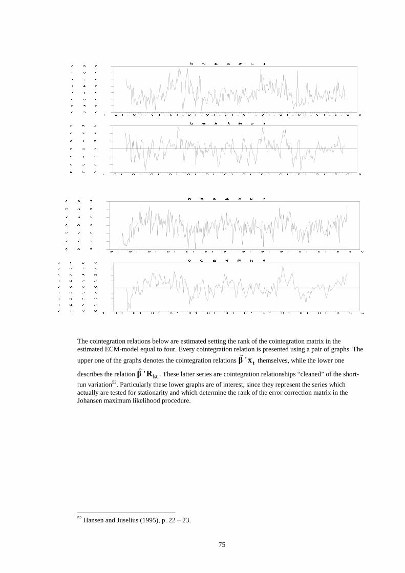
75

The cointegration relations below are estimated setting the rank of the cointegration matrix in the estimated ECM-model equal to four. Every cointegration relation is presented using a pair of graphs. The

upper one of the graphs denotes the cointegration relations tx'� themselves, while the lower one

describes the relation ktR'� . These latter series are cointegration relationships “cleaned” of the short-

run variation52. Particularly these lower graphs are of interest, since they represent the series which actually are tested for stationarity and which determine the rank of the error correction matrix in the Johansen maximum likelihood procedure.

52 Hansen and Juselius (1995), p. 22 – 23.

� �� � ��� �� � ������ �� ��

� � �� � � �� � � �� � � �� � � �� � � �� � � � � � �� � � !� � � �� � � �� � � � � � �"# $ %

"# & '

"# & %

"# ( '

"# ( %

"# ) '

"# ) %

* +* + ,,- .- . /0/011 22 3,43,4

5 6 7 85 6 7 95 6 7 :5 6 : ;5 6 : <5 6 : 85 6 : 95 6 : :5 6 6 ;5 6 6 <5 6 6 85 6 6 95 6 6 :=> ? > >=> > @ A=> > A >=> > B A=> > > >=> > B A=> > A >=> > @ A=> ? > >

CC DD EEFF GG HIHIJJ KK LEMLEM

N O P QR S T UV W X YZ [ \ ]^ _ ` a^ _ ` b^ _ ` c^ _ ` `^ _ _ d^ _ _ a^ _ _ b^ _ _ c^ _ _ `e fg e

h ij h

h ik h

l il h

l im h

l in h

o ih h

p qr s

tt uu vvww xx yzyz{{ || }v~}v~

� � � �� � � �� � � �� � � �� � � �� � � �� � � �� � � �� � � �� � � �� � � �� � � �� � � ��� �� �

�� �� �

�� �� �

�� �� �

� �� �

� �� �

� �� �

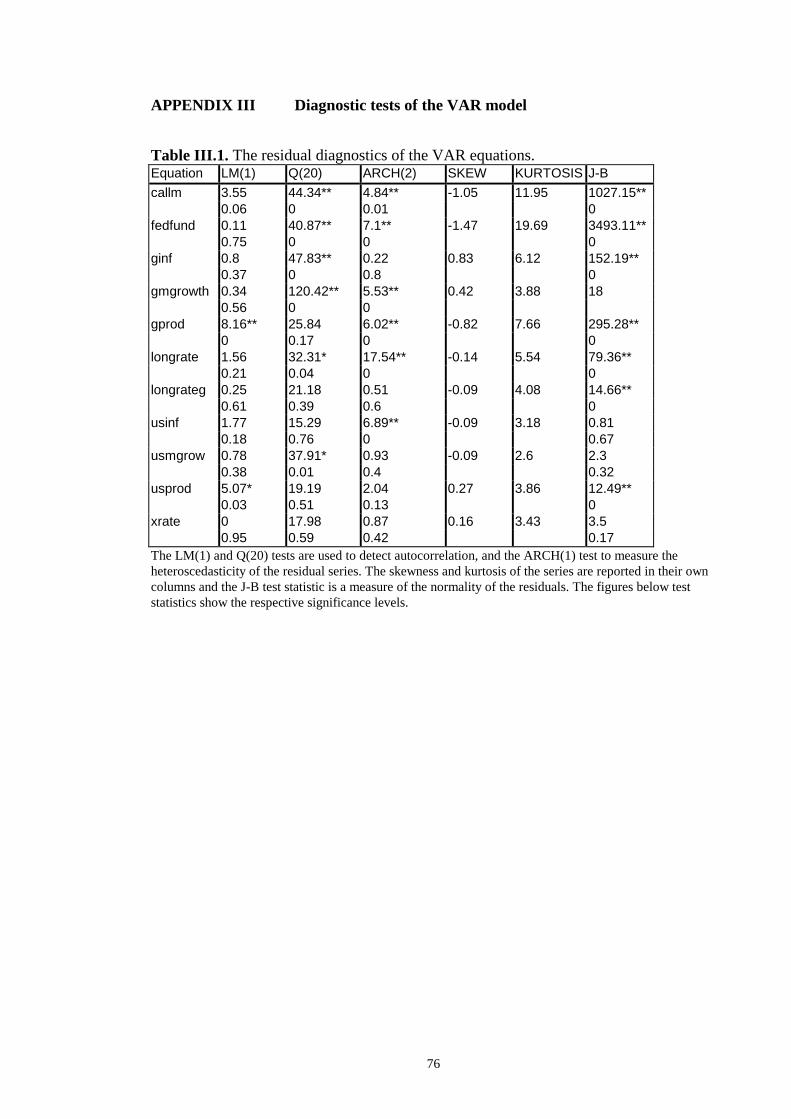
76

APPENDIX III Diagnostic tests of the VAR model

Table III .1. The residual diagnostics of the VAR equations. Equation LM(1) Q(20) ARCH(2) SKEW KURTOSIS J-B

callm 3.55 44.34** 4.84** -1.05 11.95 1027.15** 0.06 0 0.01 0

fedfund 0.11 40.87** 7.1** -1.47 19.69 3493.11** 0.75 0 0 0

ginf 0.8 47.83** 0.22 0.83 6.12 152.19** 0.37 0 0.8 0

gmgrowth 0.34 120.42** 5.53** 0.42 3.88 18 0.56 0 0

gprod 8.16** 25.84 6.02** -0.82 7.66 295.28** 0 0.17 0 0

longrate 1.56 32.31* 17.54** -0.14 5.54 79.36** 0.21 0.04 0 0

longrateg 0.25 21.18 0.51 -0.09 4.08 14.66** 0.61 0.39 0.6 0

usinf 1.77 15.29 6.89** -0.09 3.18 0.81 0.18 0.76 0 0.67

usmgrow 0.78 37.91* 0.93 -0.09 2.6 2.3 0.38 0.01 0.4 0.32

usprod 5.07* 19.19 2.04 0.27 3.86 12.49** 0.03 0.51 0.13 0

xrate 0 17.98 0.87 0.16 3.43 3.5 0.95 0.59 0.42 0.17

The LM(1) and Q(20) tests are used to detect autocorrelation, and the ARCH(1) test to measure the heteroscedasticity of the residual series. The skewness and kurtosis of the series are reported in their own columns and the J-B test statistic is a measure of the normality of the residuals. The figures below test statistics show the respective significance levels.

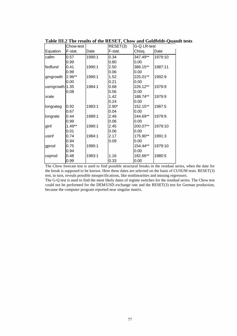
77

Table III .2 The results of the RESET, Chow and Goldfeldt-Quandt tests Chow-test RESET(3) G-Q LR-test

Equation F-stat. Date F-stat. Chisq. Date

callm 0.57 1990:1 0.34 347.49** 1979:10 0.99 0.80 0.00

fedfund 0.41 1990:1 2.50 386.15** 1987:11 0.99 0.06 0.00

gmgrowth 2.96** 1990:1 1.52 225.01** 1992:9 0.00 0.21 0.00

usmgrowth 1.35 1984:1 0.68 226.12** 1979:9 0.08 0.56 0.00

xrate 1.42 188.74** 1979:9 0.24 0.00

longrateg 0.92 1983:1 2.90* 152.15** 1987:5 0.67 0.04 0.00

longrate 0.44 1989:1 2.49 244.69** 1979:9 0.99 0.06 0.00

ginf 1.49** 1990:1 2.45 200.07** 1979:10 0.01 0.06 0.00

usinf 0.74 1984:1 2.17 175.90** 1991:3 0.94 0.09 0.00

gprod 0.75 1990:1 154.44** 1979:10 0.94 0.00

usprod 0.48 1983:1 1.16 182.66** 1980:5 0.99 0.33 0.00

The Chow forecast test is used to find possible structural breaks in the residual series, when the date for the break is supposed to be known. Here these dates are selected on the basis of CUSUM tests. RESET(3) test, in turn, reveals possible misspecifications, like nonlinearities and missing regressors. The G-Q test is used to find the most likely dates of regime switches for the residual series. The Chow test could not be performed for the DEM/USD exchange rate and the RESET(3) test for German production, because the computer program reported near singular matrix.

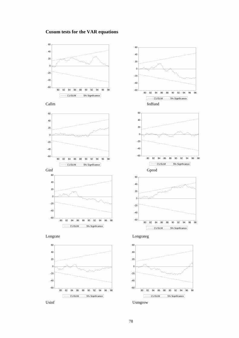
78

Cusum tests for the VAR equations Callm fedfund Ginf Gprod Longrate Longrateg Usinf Usmgrow

-60

-40

-20

0

20

40

60

80 82 84 86 88 90 92 94 96 98

CUSUM 5% Significance

-60

-40

-20

0

20

40

60

80 82 84 86 88 90 92 94 96 98

CUSUM 5% Significance

-60

-40

-20

0

20

40

60

80 82 84 86 88 90 92 94 96 98

CUSUM 5% Significance

-60

-40

-20

0

20

40

60

80 82 84 86 88 90 92 94 96 98

CUSUM 5% Significance

-60

-40

-20

0

20

40

60

80 82 84 86 88 90 92 94 96 98

CUSUM 5% Significance

-60

-40

-20

0

20

40

60

80 82 84 86 88 90 92 94 96 98

CUSUM 5% Significance

-60

-40

-20

0

20

40

60

80 82 84 86 88 90 92 94 96 98

CUSUM 5% Significance

-60

-40

-20

0

20

40

60

80 82 84 86 88 90 92 94 96 98

CUSUM 5% Significance

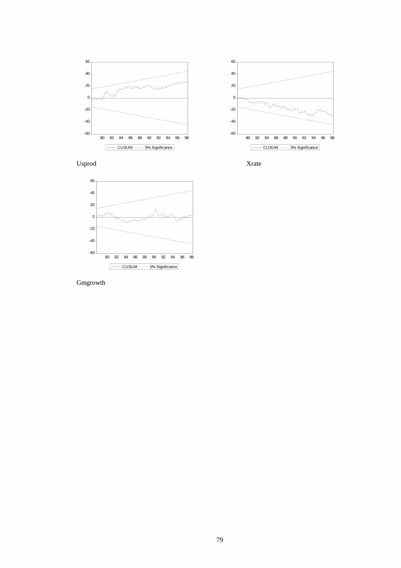
79

Usprod Xrate Gmgrowth

-60

-40

-20

0

20

40

60

80 82 84 86 88 90 92 94 96 98

CUSUM 5% Significance

-60

-40

-20

0

20

40

60

80 82 84 86 88 90 92 94 96 98

CUSUM 5% Significance

-60

-40

-20

0

20

40

60

80 82 84 86 88 90 92 94 96 98

CUSUM 5% Significance

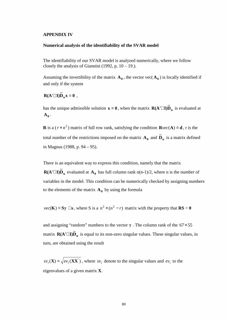
80

APPENDIX IV Numerical analysis of the identifiabili ty of the SVAR model

The identifiabilit y of our SVAR model is analyzed numerically, where we follow closely the analysis of Giannini (1992, p. 10 – 19.).

Assuming the invertibilit y of the matrix 0A , the vector vec( 0A ) is locally identified if

and only if the system

0xDI)R(A' n =⊗ ~ ,

has the unique admissible solution 0x = , when the matrix nDI)R(A'~⊗ is evaluated at

0A .

R is a ( 2nr × ) matrix of full row rank, satisfying the condition dAR =)(vec , r is the

total number of the restrictions imposed on the matrix 0A and nD~

is a matrix defined

in Magnus (1988, p. 94 – 95).

There is an equivalent way to express this condition, namely that the matrix

nDI)R(A'~⊗ evaluated at 0A has full column rank n(n-1)/2, where n is the number of

variables in the model. This condition can be numerically checked by assigning numbers

to the elements of the matrix 0A by using the formula

sS�K +=)(vec , where S is a )( 22 rnn −× matrix with the property that RS = 0

and assigning “ random” numbers to the vector � . The column rank of the 5567×

matrix nDI)R(A'~⊗ is equal to its non-zero singular values. These singular values, in

turn, are obtained using the result

)()( 'XXX ii evsv = , where isv denote to the singular values and iev to the

eigenvalues of a given matrix X.

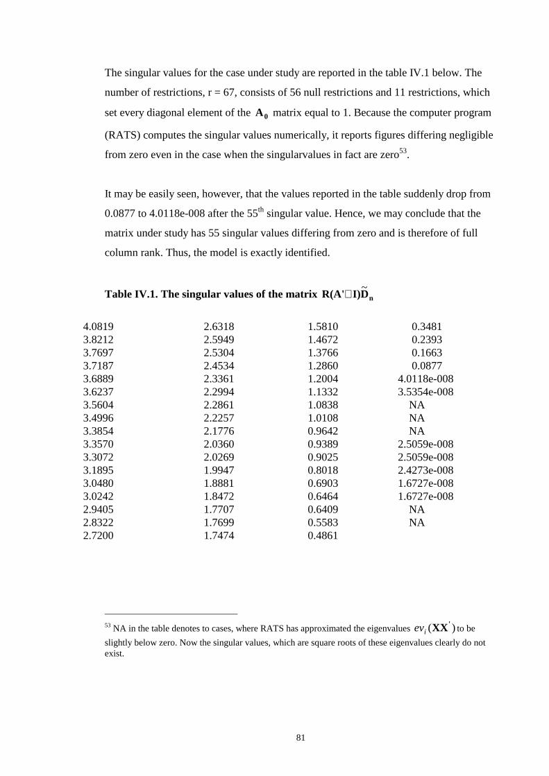
81

The singular values for the case under study are reported in the table IV.1 below. The

number of restrictions, r = 67, consists of 56 null restrictions and 11 restrictions, which

set every diagonal element of the 0A matrix equal to 1. Because the computer program

(RATS) computes the singular values numerically, it reports figures differing negligible

from zero even in the case when the singularvalues in fact are zero53.

It may be easily seen, however, that the values reported in the table suddenly drop from

0.0877 to 4.0118e-008 after the 55th singular value. Hence, we may conclude that the

matrix under study has 55 singular values differing from zero and is therefore of full

column rank. Thus, the model is exactly identified.

Table IV.1. The singular values of the matr ix nDI)R(A'~⊗

53 NA in the table denotes to cases, where RATS has approximated the eigenvalues )( 'XXiev to be

slightly below zero. Now the singular values, which are square roots of these eigenvalues clearly do not exist.

4.0819 3.8212 3.7697 3.7187 3.6889 3.6237 3.5604 3.4996 3.3854 3.3570 3.3072 3.1895 3.0480 3.0242 2.9405 2.8322 2.7200

2.6318 2.5949 2.5304 2.4534 2.3361 2.2994 2.2861 2.2257 2.1776 2.0360 2.0269 1.9947 1.8881 1.8472 1.7707 1.7699 1.7474

1.5810 1.4672 1.3766 1.2860 1.2004 1.1332 1.0838 1.0108 0.9642 0.9389 0.9025 0.8018 0.6903 0.6464 0.6409 0.5583 0.4861

0.3481 0.2393 0.1663 0.0877 4.0118e-008 3.5354e-008 NA NA NA 2.5059e-008 2.5059e-008 2.4273e-008 1.6727e-008 1.6727e-008 NA NA

82

CHAPTER 3

Regime Switches in the Reaction Functions of the Federal Reserve and the Bundesbank in the post Bretton Woods era

Abstract The purpose of this paper is to study whether there were sudden changes in the parameter values of the Taylor rule type reaction function of the Federal Reserve and Bundesbank during the period 1970 – 1998. The reaction functions are estimated as Markov switching models with state dependent coeff icients. The robustness of the results on the exact specification of the policy rule and on the measure for inflation and the output gap used in the estimation are examined by considering several alternative data sets and model specifications in the estimations. According to the results it is possible to characterize the behaviour of the Fed as a switching between two regimes with different weights put on resisting inflation and stabili zing fluctuations in output. The regimes of the Bundesbank, in turn, were classified as a regime without any response to either inflation or output gap, and a regime when the Bundesbank responded to both of the gaps. On the other hand, the results supported some previous findings according to which Taylor-type policy rule estimations are sensitive to the specification of the rule and the choice of the data. KEY WORDS: monetary policy rules, Markov-switching models, data uncertainty.

JEL Classification: C82, E42, E52, E58

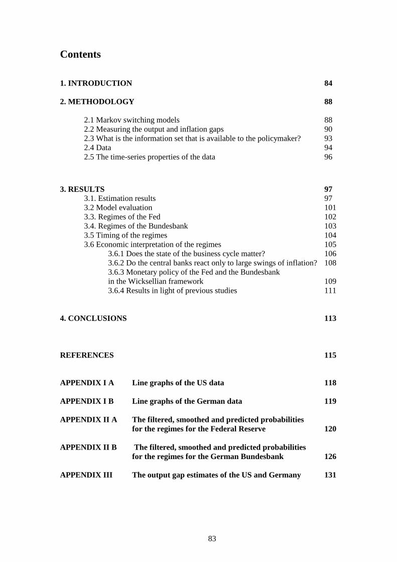
83

Contents 1. INTRODUCTION 84 2. METHODOLOGY 88 2.1 Markov switching models 88 2.2 Measuring the output and inflation gaps 90 2.3 What is the information set that is available to the policymaker? 93 2.4 Data 94 2.5 The time-series properties of the data 96

3. RESULT S 97 3.1. Estimation results 97 3.2 Model evaluation 101 3.3. Regimes of the Fed 102 3.4. Regimes of the Bundesbank 103 3.5 Timing of the regimes 104 3.6 Economic interpretation of the regimes 105 3.6.1 Does the state of the business cycle matter? 106 3.6.2 Do the central banks react only to large swings of inflation? 108

3.6.3 Monetary policy of the Fed and the Bundesbank in the Wickselli an framework 109 3.6.4 Results in light of previous studies 111

4. CONCLUSIONS 113 REFERENCES 115 APPENDIX I A L ine graphs of the US data 118 APPENDIX I B L ine graphs of the German data 119 APPENDIX II A The fil tered, smoothed and predicted probabili ties

for the regimes for the Federal Reserve 120 APPENDIX II B The fil tered, smoothed and predicted probabili ties

for the regimes for the German Bundesbank 126 APPENDIX III The output gap estimates of the US and Germany 131

84

1. INTRODUCTION

Many macroeconomic studies involve modelli ng central bank behaviour in terms of a single,

stable reaction function. For example, the literature on the effects of monetary policy shocks

based on vector-autoregressive models is implicitl y based on estimating such a rule. Macro

models with rational expectations provide another example, because knowing the correct

policy rule is an important element of estimating the entire model. Since the publication of the

seminal paper by Taylor (1993), it has become a common practice to model central bank

behaviour on a rule that relates short-term nominal interest rate to deviations of inflation and

output from their desired values.

The interpretation of such a rule is straightforward: Because the monetary policy is transmitted

to the economy through changes in the real interest rate, it is the real rate which is the ultimate

target variable of the central bank. When output and inflation are at their desired levels, the

central bank sets its policy rate equal to the sum of the equili brium real interest rate and

inflation target. When the inflation is above its target or output is above its potential, the real

interest rate will be increased above its equili brium level by the central bank to calm down the

overheated economy. Similarly, in the case of deflation and high unemployment the real

interest rate is decreased.

It is however not always wise to blindly assume the existence of a stable, linear decision rule

for a central bank, since there might have happened regime changes during the sample period

that have to be taken into account when estimating these policy rule (see e.g. Judd and

Rudebusch 1998). Thus, the purpose of this study is to examine potential regime shifts in the

monetary policy reaction functions of the Federal Reserve and the German Bundesbank during

the post Bretton-Woods period of 1970 - 1998.

The motivation of the study is twofold. First, our approach differs from the previous literature

on regime changes in central bank policy rules in that now the timing of the possible regime

breaks is endogenised, whereas the previous studies have assumed that the dates of possible

regime changes are known a priori. Thus, instead of dividing the sample period into sub-

periods and estimating a different linear model for each period, I estimate Markov switching

(MS) models, which allow for discrete regime shifts among a set of alternative parameter

85

values in the central bank reaction function at different points in time. Secondly, the study

discusses the robustness of the estimation results on exact specification of the rule and the way

the inflation and output gap are measured. Using linear models, the issue has previously been

studied e.g. by Orphanides (1997) and Kozicki (1999) and Cerra et al. (2000). Perhaps the

most well -known of these studies is Orphanides (1997) who found that the Taylor rule

estimates are sensitive on whether the estimations are based on real-time data available to the

policymaker at the moment the stance of monetary policy was set. Kozicki (1999) and Cerra et

al. (2000) in turn studied the robustness of the Taylor rule estimates with respect to the way

the output gap has been defined. Kozicki (1999) also examines the robustness issue with

respect to a number of modifications of the rule, including the way the inflation is measured

and whether the estimated rule includes an interest rate smoothing term or not.

Although the MS models are based on endogenising the timing of the regime shifts, some less

formal prior knowledge about the possible regime changes is used for evaluating the

plausibilit y of the results. The important institutional events that have occurred during the

sample period include e.g. introducing the currency snake system in 1972, which was followed

by the more rigid ERM system later in 1979. The reunification of Germany at the turn of

1990’s also took place during the sample period. In the case of the US, the most important

potential regime shifts include at least the changes in the operating procedures of the Federal

Reserve during the years 1979-1982 and 1984.

It is important to note that the changes in parameter values of the policy rule do not

necessarily directly link to concurrent changes in the underlying preference parameters

describing the relative weights of inflation and output variabilit y in the policymaker’s welfare

function. Instead, the regime changes may reflect changes in the transmission mechanism of

the monetary policy, observed by the policymaker. If there is, for example, a regime switch in

the channel through which the monetary policy affects the economy, a welfare maximizing

policymaker might have to raise interest rates just in order to keep inflation variabilit y at its

previous level.

In the previous literature, Taylor (1998), Judd and Rudebusch (1998) and Clarida et al. (2000)

are examples of previous attempts to detect regime changes in the US monetary policy in a

Taylor rule framework. Taylor (1998) focuses on changes in the Fed’s policy rule in a longer

perspective examining several episodes with different monetary policy regimes. He concludes

86

that a simple interest rate rule, in which the interest rate responds to changes in inflation and

output, is a useful framework for examining the U.S. monetary history, since the simple policy

rule may be implied by many different monetary systems. It was found that the Fed’s policy

rule has changed dramatically from the early periods of gold standard to the fixed exchange

rate regime in the Bretton-Woods era and the modern flexible exchange rate era. The

conclusion is that a good policy rule is characterized as one in which the interest rate responds

to deviations in inflation and output relatively aggressively, as during the 1980s and 1990s.

Judd and Rudebusch (1998)1 in turn, try to find changes in the Fed’s reaction function

resulting from compositional changes in the Federal Open Market Committee. Judd and

Rudebusch divide their sample period (1970:1 – 1997:4) into three sub-periods according to

the respective chairmen of the Fed. Then, a Taylor-rule type reaction function is estimated for

each of the sub-periods. According to the results, Greenspan’s (1987:3 – 1997:4) period has

been the one that could best be characterized by a Taylor rule type feedback rule. For

Volcker’s period (1979:3 – 1987:2) the estimates were less precise, but they suggested an

implicit inflation target well below that inherited from the late 1970’s. Finally, in the Burns

period (1970:1 – 1978:2) the link between inflation and monetary policy seemed to respond

more to the state of business cycle than to inflation. The authors conclude that a Taylor-rule

framework is a useful tool for the description of the key elements of monetary policy.

Clarida et al. (2000) finally, detect differences in the Fed’s policy regimes between the periods

before and after Volcker’s appointment as a chairman of the Fed. A forward-looking reaction

function is estimated and the estimated parameter values are discussed in light of a small

quantitative macromodel. Some sources of instabilit y were found from the Fed’s monetary

policy during the pre-Volcker period, when monetary policy seemed to be accommodating

increased inflation.

Ang and Bekaert (1998), Sill and Wrase (1999) and Linde (2000) provide examples of studies

on regime changes in the monetary policy that are based on a different approach than the

Taylor rule framework. Ang and Bekaert (1998) study the non-linearities in the behaviour of

the short-term interest rates of the US, Germany and UK using a multivariate Markov-

switching framework. Instead of estimating reaction functions for the central banks, the

87

authors use the term spread and international interest rates as well as the own history of the

short rate as explanatory variables. It is concluded that the regime switching models

outperform their linear counterparts when it comes to forecasting. On the other hand, due to

small sample problems with the regime switching models, the moments implied by the linear

models tend to fit the data better than those of regime switching models.

Sill and Wrase (1999) examine the regime changes in the joint money supply processes of the

US and Canada by estimating a Markov-Switching VAR model. According to the results,

there have been two regime changes during the sample period. In the middle of 1971, there

seems to have been a switch from a high monetary growth regime to a low growth regime. In

mid 1981, the policy returned to the high growth regime again. Linde (2000) in turn, examines

the parameter changes of the Fed’s reaction function during the periods of different chairmen.

Linde uses the monetary base instead of the short-term interest rate as the dependent variable

when he estimates his reaction functions for the periods of the different chairmen. The results

corroborate the finding that the Fed has adjusted the monetary base most radically in response

to inflation during Greenspan’s period. During Burn’s chairmanship the response was at its

lowest.

The previous empirical studies on the monetary policy rules of Germany include e.g. Clarida

and Gertler (1996), Clarida et al. (1998) and Peersman and Smets (1999). All the studies,

however, estimate only a single linear rule, paying no attention to the possible regime breaks.

The main findings of Clarida and Gertler are, firstly, that despite the publicly announced focus

on monetary targeting, the German monetary policy also involved managing short-term

interest rates, while the monetary targets provide only one of the reference points for the

policy. Further, the authors suggest that while achieving and maintaining low inflation was the

main concern for German monetary authorities, the Bundesbank at least implicitl y has also

pursued countercyclical monetary policy. That is, it has adopted more or less gradualist

approach to disinflating, being ready to ease the monetary policy when the real economy has

weakened.

Overall , Clarida and Gertler found that German monetary policy can be characterized by a

modified forward looking Taylor type feedback rule. The estimated coeff icients in the basic

1 The article can be downloaded from the web site of the Federal Reserve Bank of San Francisco:

88

specification for the response of the call money rate was 0.78 on changes in the inflation gap2

and 0.64 on output gap, when the full sample period was considered. Clarida and Gertler,

however, found evidence of asymmetry in the Bundesbank’s reactions to inflation. When the

inflation has levelled above its target value, the Bundesbank has reacted to inflation more

aggressively than during the periods with negative inflation gap. Thus, the study by Clarida

and Gertler can also be interpreted as providing evidence about the existence of two separate

regimes in the Bundesbank’s monetary policy.

Clarida et al. (1998), in turn, estimate reaction functions for all G3 countries after 1979. The

authors find evidence of an implicit form of inflation targeting with interest rate smoothing

and some allowance for output stabili zation. Further, the results again suggest that the central

banks respond anticipated rather than to lagged inflation. This hypothesis of the forward

lookingness of the Bundesbank’s monetary policy was, however, called into question by

Peersman and Smets (1998). When they re-estimated the study by Clarida et al. (1998) they

found that the coeff icient of current inflation remained significant when added to the baseline

specification. Instead, the two-year ahead annual inflation did not. This finding cast some

doubt on the interpretation that the Bundesbank cares also about stabili zing output.

2. METHODOLOGY

2.1 Markov switching models

Markov switching models are based on the idea that the parameter values of the empirical

model are driven by two or more unobservable states ( ts ) that follow first-order Markov

process. In our set-up, specifically, each state ( ts ) corresponds to some specific set of

parameters in the central bank reaction function under estimation. Intuitively, the states can

now be interpreted as indicating stronger or weaker responses to changes in the inflation or

http://www.frbsf.org/econrsrch/econrev/index.1998.html 2 These estimated low coeff icients for the inflation gap may perhaps be interpreted as a sign of “non Wickselli an” monetary policy during the estimation period. The definition and the problems of the non-Wickselli an monetary policy will be addressed in more detail l ater when the estimation results are discussed.

89

output gap. More formally, the Markov switching models considered in this study take the

form of (2.1) representing a single equation Markov switching model.

(2.1) st0ststst

at

y ++= xb ' , s = 1,2 and t=1, …, T

where ty is the dependent variable, sta is the state-dependent constant term, stx is a vector of

explanatory variables, stb is a vector of coeff icients and stε is the state-dependent error term.

The economy is assumed to be in either of the two states, which change with the probabiliti es

111 p− and 221 p− , while 11p and 22p give the probabilit y of staying at a given state ts

during period t+1, if it has been reached at period t. More compactly, the transition

probabiliti es are summarized by Markov matrix

−

−=

2211

2211

1

1

pp

ppP , where ijp =Pr )( 1 isjs tt ==+

The estimation of the Markov switching methods is carried out by maximum likelihood

method. Thus, the error terms of the model are assumed to be normally distributed.

The relation between the empirical model (2.1) and the Taylor rule becomes clear by writing

our baseline specification for the rule as

(2.2) )()( **** yyrit −+−++= βππαπ ,

where ti =nominal interest rate, *r =the real interest rate target of the central bank,

*π =inflation target of the central bank, ty =real output, *ty =the natural level of output and α

and β are parameters. Thus, the vector of explanatory variables in the eq. (2.1) consists of

inflation gap )( *ππ − and output gap )( *yy − , while the constant term is made up of the sum

of the real interest rate target and the inflation target ( ** π+r ).

90

Before estimating a Taylor-type central bank reaction function, one has to take a stand on

some problems related to the selection of the data. The problems include questions such as

how to correctly measure the output and inflation gaps of the economy, or what information

set was available to the policy maker at the time the policy decisions were made? Should one

use lagged or current values of inflation and output gaps as explanatory variables? Because

there are no definitive answers to most of these questions, and in order to examine the

robustness of the results on the different solution to these problems, several alternative model

specifications are estimated.

2.2 Measur ing the output and inflation gaps

The problems with measuring the natural level of output, even for a single point of time, are

well known. These problems are further highlighted here, because the natural level of output

has likely changed substantially during the relatively long sample period. A commonly applied

practice to obtain a crude measure of the potential output is simply to apply time-series

methods like fitting a linear or quadratic trend to the data or to use Hodrick-Prescott filtering.

These procedures are implicitl y based on the notion that the deviations of the output of its

potential level are always transitory and average out in the long run. The unobserved-

components methods, such as the univariate or multivariate Beveridge-Nelson decomposition

are based on estimating unobserved variables, such as potential output or the NAIRU, using

information from observed variables. The structural VAR method, in turn, identifies potential

output with the aggregate supply capacity of the economy and cyclical fluctuations with

changes in aggregate demand.

Central banks or organizations like IMF and OECD use more elaborate structural economic

models. The production-function approach, for instance, is based on estimating the economy’s

aggregate production function e.g. in the Cobb-Douglas form. The sensitivity of the parameter

values of the estimated Taylor’s rule on different methods of measuring the potential output

has been examined by Kozicki (1999). Cerra et al. (2000) in turn, compare the pros and cons

of six differing methodologies to measure the potential output, with an application to Swedish

data. Both studies suggest that the parameter estimates for the Taylor rule may be sensitive to

the methodology that is used to estimate the output gap. None of the competing methods for

measuring the output gap was considered superior to the others, however. In this study, two

91

alternative estimates of the potential output are used in the case of both countries. The first

estimates are based on structural economic methods, while the alternative measure of the

potential output is obtained by Hodrick-Prescott filtering the data. In the case of the U.S.

economy the structural estimates of the output gap were published by the US Congressional

Budget Off ice (CBO) and in the case of Germany the structural estimates are from the OECD

Economic Outlook database.3

Kozicki (1999) discussed the correct choice between various measures of inflation when

estimating the parameters of the policy rule of the Fed. He found that the estimates of the

parameters of the Taylor’s rule are also sensitive on the way the inflation is measured. When

the Taylor’s rule was estimated with the US data for a sample period of 1983 – 1997 with four

different inflation measures (CPI, core CPI, GDP deflator, expected inflation) the best fit was

obtained in a model with expected inflation. The finding suggests that central banks may be

forward looking when setting the policy instrument. The results are also in line with the

somewhat controversial results of Clarida et al. (1998) cited above, according to which at least

the Bundesbank has been forward-looking when setting its monetary policy.

In this study, both backward-looking and forward-looking policy rules are estimated. In the

forward looking models, the inflation expectations for the US are based on professional

forecasters’ forecasts of the U.S. GDP inflation, while for Germany the inflation expectations

were CPI inflation forecasts published by the OECD. The backward looking data consist of

the realized values of these same inflation measures.4

Neither the Fed nor the Bundesbank have had any publicly announced, explicit inflation target

for the sample period. Thus, some implicit measures for the inflation targets have to be found.

Clarida and Gertler (1996) calculated the inflation target by estimating a long run equili brium

level of the German inflation using a structural VAR model. Another possibilit y would be to

simply calculate long run averages of the inflation series, as was done by Judd and Rudebusch

(1998). In Clarida and Gertler (1996) the equili brium inflation of the Bundesbank was

3 The main difference between the methods of measuring the potential output seems to be, according to the visual inspection that the output gap seems to fluctuate less during the sample period when the potential output is measured by H-P filtering. 4 Obviously, the results for the Fed and the Bundesbank would have been more comparable if the inflation would have been defined and measured in the same way for both central banks. There were, however, problems in obtaining the series for the inflation expectations.

92

estimated to be 3.2 % while Judd and Rudebusch (1998) estimate that the Fed’s inflation target

has ranged between 3.03% and 6.47 % during the period 1970.Q1 – 1987.Q3, depending on

who held the chairmanship of the bank5. Obviously, the estimates for the inflation target seem

to be fairly high. A simple Barro-Gordon model, however, provides a plausible interpretation

for the high estimates of the equili brium inflation. According to the model, if the central bank

has practised some leaning against cyclical variation in the real activity during the sample

period and if the central bank’s output target has been below the potential output, then the

theory predicts that the actual inflation rate may include some premium over the target rate.

Whether or not any such inflation bias is present, depends on the central bank’s output target.6

Another problem with measuring target inflation using sample average or VAR is that these

approaches implicitl y are based on the assumption of a constant inflation target of a central

bank for the whole estimation period. Moreover, even if the sample average were calculated

separately for each sub-periods, there would still be the problem left that the inflation target

probably changes gradually, rather than in rapid discrete shifts. In this study, the problems

with calculating the inflation targets and the inflation gaps are handled by measuring the

inflation gap for both the expected and realized inflation in two different ways. The first way

is to calculate the inflation gap simply by the difference between the inflation rate (either the

expected or the realized one) and the equili brium inflation obtained by H-P filtering the data.

The second way is to avoid the calculation of the equili brium inflation and the inflation gap

altogether. This is possible by substituting for the inflation gap on the right hand side of

Equation (2.2.) with the inflation rate itself. This procedure is justified since Equation (2.2)

can always be written as Equation (2.3) below. Now the equili brium inflation only appears in

the constant term ( ** )1( πα−+r ) of that equation.

(2.3) )()1( *** yyrit −++−+= βαππα

5 Judd and Rudebusch (1998) also considered an alternative measure for the inflation target, namely the end of period level of inflation for the terms of each three chairman of the Fed. These estimates took much more reasonable values, since the inflation target for Greenspan’s era was now only 1.77 %. 6 For an interesting criticism of the inflation bias argument of Barro and Gordon, see Blinder (1999, pp. 40 – 43.)

93

2.3 What is the information set that is available to the policymaker?

Economic data usually go through considerable revisions and corrections after it has been

published for the first time. If the data available to the policymaker at the moment the policy

decisions are made are not the same than that used for the ex-post estimation of the policy

rule, severe biases in the estimates of parameters of the policy rule may follow.7 In this study

the problem is under control at least in the case of inflation, since in some of the models

inflation was measured by the inflation forecasts that were available to the policymakers at the

moment the policy decisions were made.

It is also possible to include the lagged policy instrument variable as an explanatory variable

to the policy rule specification. Many alternative interpretations for the existence of the lagged

interest rate in the monetary policy rule have been suggested. Usually the interest rate lag has

been interpreted as reflecting smoothing behaviour on the part of the central bank8 because of

the central bank’s concern about the stabilit y of the financial markets (see Kozicki (1999, pp.

8.). On the other hand, by avoiding too rapid actions in its monetary policy, the central banks

can take into account the inherent uncertainties in its information set. In addition to the sort of

uncertainty pointed out by Orphanides (1997), these uncertainties include the uncertainties

related the structure of the “true model” of the economy and the correct parameter values of

that model. As Blinder (1999) has argued, in the presence of parameter uncertainty the

policymaker should be conservative in its actions. In the study at hand, some of the alternative

policy rule specifications also contain the lagged interest rate term, which provides an

additional dimension in which to discuss the robustness of the results. As it will t urn out, the

7 The problem has been discussed e.g. by Runkle (1998), Evans (1998) and Orphanides (1997). Runkle (1998) demonstrated that the initial estimates of the output growth and inflation are not unbiased forecasts of the final estimates of these variables and that the bias may be substantial. In addition, a comparison of revision uncertainty and forecast uncertainty revealed that the former forms a significant fraction of the quite large uncertainty about forecasts of real activity and inflation. Evans (1998) tried to solve the problem by measuring inflation by the CPI instead of the GDP deflator and output by unemployment, because the information on these variables is more quickly available to the policymaker. 8 Instead of being a sign of an explicit interest rate smoothing objective, including the lagged interest rate into the reaction function may reflect an attempt of a central bank to make effects of the monetary policy more permanent. If the market participants believe that the rises and declines in the policy rates are not only a transitory phenomenon, the monetary policy becomes more effective. A related interpretation is provided by Sack (1999) who provides evidence that the observed gradualist policy of the Fed may be motivated both by the dynamic structure of the economy and the uncertainty surrounding that structure.

94

results support Kozicki (1999), who also found evidence on the sensitivity of the Taylor rule

estimates on whether the models include interest rate smoothing or not.

2.4 Data

I use quarterly data over the sample period of 1970:1 – 1998:1. As already mentioned, a

variety of different model specifications was estimated for both the Federal Reserve and the

German Bundesbank. Thus, aside from tracking the structural changes in the policy rules, the

study pursues an additional goal by extending and contributing to the discussion by Kozicki

(1999) and Cerra et al. (2000) cited above, on the robustness of the monetary policy rule

estimates on the exact specification of the rule and the way the inflation and output gap are

measured. Tables (2.1) and (2.2) on the next page summarize the features of all twelve

specifications used for both the US and Germany. The specifications differ from each other

regarding the definition of the inflation and output gaps, or with respect to whether they

include the lagged dependent variable as one of the explanatory variables or not.

The data set for the estimation of the policy rule of the Fed consists, firstly, of the federal

funds’ rate that represents the Fed’s policy instrument. The inflation gap variable is defined as

the difference between the GDP inflation and the equili brium inflation estimated by H-P

filtering9. The inflation is defined either as the realized GDP inflation (backward looking

specifications) or as the expected inflation (forward looking specifications). In addition to the

explicitl y calculated inflation gap series, the inflation variable itself is used as an explanatory

variable in some of the specifications. When estimating the forward looking models, two

different estimates of the output gap are used. The first measure is based on the potential

output estimate provided by the Congressional Budget Off ice of the US (CBO), while the

second one is based on the potential output gap calculated by H-P filtering. In all of the

backward looking specifications the output gap is defined as the CBO estimates.

For Germany, I use call money rate as representing the Bundesbank’s monetary policy

instrument. Again, the policy rules are estimated both as backward and forward looking

9 The series for the inflation expectations are the Livingston survey data published by the Federal Reserve Bank of Philadelphia.

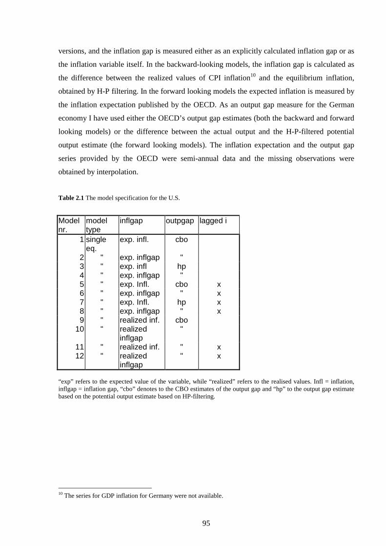
95

versions, and the inflation gap is measured either as an explicitl y calculated inflation gap or as

the inflation variable itself. In the backward-looking models, the inflation gap is calculated as

the difference between the realized values of CPI inflation10 and the equili brium inflation,

obtained by H-P filtering. In the forward looking models the expected inflation is measured by

the inflation expectation published by the OECD. As an output gap measure for the German

economy I have used either the OECD’s output gap estimates (both the backward and forward

looking models) or the difference between the actual output and the H-P-filtered potential

output estimate (the forward looking models). The inflation expectation and the output gap

series provided by the OECD were semi-annual data and the missing observations were

obtained by interpolation.

Table 2.1 The model specification for the U.S.

Model nr.

model type

inflgap outpgap lagged i

1 single eq.

exp. infl. cbo

2 " exp. inflgap " 3 " exp. infl hp 4 " exp. inflgap " 5 " exp. Infl. cbo x 6 " exp. inflgap " x 7 " exp. Infl. hp x 8 " exp. inflgap " x 9 " realized inf. cbo

10 " realized inflgap

"

11 " realized inf. " x 12 " realized

inflgap " x

“exp” refers to the expected value of the variable, while “realized” refers to the realised values. Infl = inflation, inflgap = inflation gap, “cbo” denotes to the CBO estimates of the output gap and “hp” to the output gap estimate based on the potential output estimate based on HP-filtering.

10 The series for GDP inflation for Germany were not available.

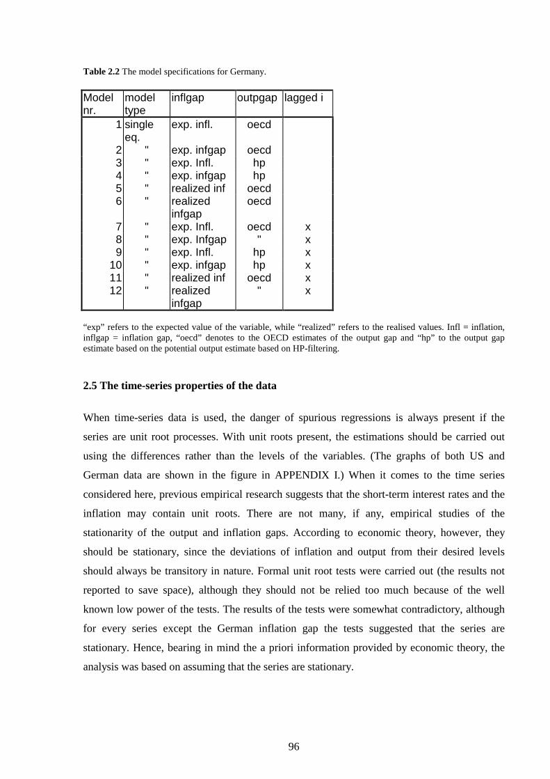
96

Table 2.2 The model specifications for Germany. Model nr.

model type

inflgap outpgap lagged i

1 single eq.

exp. infl. oecd

2 " exp. infgap oecd 3 " exp. Infl. hp 4 " exp. infgap hp 5 " realized inf oecd 6 " realized

infgap oecd

7 " exp. Infl. oecd x 8 " exp. Infgap " x 9 " exp. Infl. hp x

10 " exp. infgap hp x 11 " realized inf oecd x 12 " realized

infgap " x

“exp” refers to the expected value of the variable, while “realized” refers to the realised values. Infl = inflation, inflgap = inflation gap, “oecd” denotes to the OECD estimates of the output gap and “hp” to the output gap estimate based on the potential output estimate based on HP-filtering. 2.5 The time-series properties of the data

When time-series data is used, the danger of spurious regressions is always present if the

series are unit root processes. With unit roots present, the estimations should be carried out

using the differences rather than the levels of the variables. (The graphs of both US and

German data are shown in the figure in APPENDIX I.) When it comes to the time series

considered here, previous empirical research suggests that the short-term interest rates and the

inflation may contain unit roots. There are not many, if any, empirical studies of the

stationarity of the output and inflation gaps. According to economic theory, however, they

should be stationary, since the deviations of inflation and output from their desired levels

should always be transitory in nature. Formal unit root tests were carried out (the results not

reported to save space), although they should not be relied too much because of the well

known low power of the tests. The results of the tests were somewhat contradictory, although

for every series except the German inflation gap the tests suggested that the series are

stationary. Hence, bearing in mind the a priori information provided by economic theory, the

analysis was based on assuming that the series are stationary.

97

3. RESULT S

3.1 Estimation results

All models were estimated using maximum likelihood method ultimately based on Hamilton

(1994). The estimations were carried out using MSVAR package for Ox, which applies the

EM algorithm. If the economic relationships to be modelled could be adequately characterized

by a linear model, there is no sense in estimating a non-linear model, li ke the Markov

switching model. Thus, the estimations were started by comparing the adequacy of the linear

model against the Markov switching model using both the conventional AIC and SBC

information criteria as well as the LR tests. Using the LR tests is actually problematic, since

the parameters 11p and 22p appear only in the MS model but not in the linear model. The

information matrix of the model with two states would then be singular if the null hypothesis

of only one state holds. Accordingly, the asymptotic distribution of the LR test is not known11.

The problem was handled by using the conservative 2χ (1) distribution. The LR tests still

always suggested that the hypothesis of a linear model should be rejected at 99 % confidence

level. The information criteria also suggested estimating a non-linear model.

The number of states in the Markov switching model was chosen to be two for the models for

both the Fed and the Bundesbank. Actually, the information criteria suggested models with

three states, but these models turned out to be too diff icult to interpret, mainly because of the

very ragged shapes of the line graphs of the smoothed probabiliti es of the regimes. The

Markov switching modelli ng also allows for estimation of the error term variance separately

for each of the states, which is clearly an advantage in our estimation. The assumption of a

constant variance is not likely to hold for short-term interest rates as it is the case for also

many other financial time series. The estimated parameter values for the policy rules of the

Fed and the Bundesbank are presented in Tables 3.1 and 3.2 below. The timing of the regimes

is represented by the time paths of the filtered, smoothed and predicted probabiliti es of the two

regimes that are shown in Appendix II . The filtered probabilit y is the optimal inference on the

state variable at time t using only the information up to time t, i.e. )Pr( tt Yms = ). The

smoothed probabilit y refers to the optimal inference on the state variable at time t using the

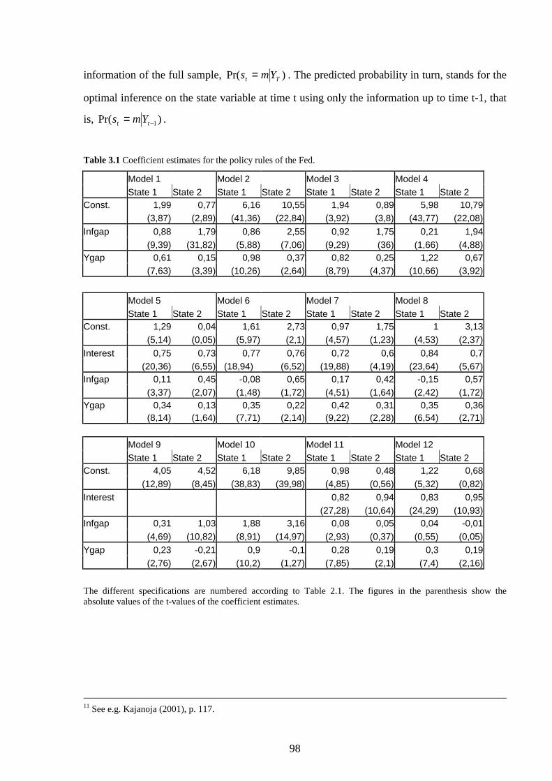
98

information of the full sample, )Pr( Tt Yms = . The predicted probabilit y in turn, stands for the

optimal inference on the state variable at time t using only the information up to time t-1, that

is, )Pr( 1−= tt Yms .

Table 3.1 Coeff icient estimates for the policy rules of the Fed.

Model 1 Model 2 Model 3 Model 4 State 1 State 2 State 1 State 2 State 1 State 2 State 1 State 2 Const. 1,99 0,77 6,16 10,55 1,94 0,89 5,98 10,79 (3,87) (2,89) (41,36) (22,84) (3,92) (3,8) (43,77) (22,08)

Infgap 0,88 1,79 0,86 2,55 0,92 1,75 0,21 1,94 (9,39) (31,82) (5,88) (7,06) (9,29) (36) (1,66) (4,88) Ygap 0,61 0,15 0,98 0,37 0,82 0,25 1,22 0,67 (7,63) (3,39) (10,26) (2,64) (8,79) (4,37) (10,66) (3,92)

Model 5 Model 6 Model 7 Model 8 State 1 State 2 State 1 State 2 State 1 State 2 State 1 State 2 Const. 1,29 0,04 1,61 2,73 0,97 1,75 1 3,13 (5,14) (0,05) (5,97) (2,1) (4,57) (1,23) (4,53) (2,37)

Interest 0,75 0,73 0,77 0,76 0,72 0,6 0,84 0,7 (20,36) (6,55) (18,94) (6,52) (19,88) (4,19) (23,64) (5,67) Infgap 0,11 0,45 -0,08 0,65 0,17 0,42 -0,15 0,57 (3,37) (2,07) (1,48) (1,72) (4,51) (1,64) (2,42) (1,72) Ygap 0,34 0,13 0,35 0,22 0,42 0,31 0,35 0,36 (8,14) (1,64) (7,71) (2,14) (9,22) (2,28) (6,54) (2,71)

Model 9 Model 10 Model 11 Model 12 State 1 State 2 State 1 State 2 State 1 State 2 State 1 State 2 Const. 4,05 4,52 6,18 9,85 0,98 0,48 1,22 0,68 (12,89) (8,45) (38,83) (39,98) (4,85) (0,56) (5,32) (0,82)

Interest 0,82 0,94 0,83 0,95 (27,28) (10,64) (24,29) (10,93) Infgap 0,31 1,03 1,88 3,16 0,08 0,05 0,04 -0,01 (4,69) (10,82) (8,91) (14,97) (2,93) (0,37) (0,55) (0,05)

Ygap 0,23 -0,21 0,9 -0,1 0,28 0,19 0,3 0,19 (2,76) (2,67) (10,2) (1,27) (7,85) (2,1) (7,4) (2,16)

The different specifications are numbered according to Table 2.1. The figures in the parenthesis show the absolute values of the t-values of the coeff icient estimates.

11 See e.g. Kajanoja (2001), p. 117.

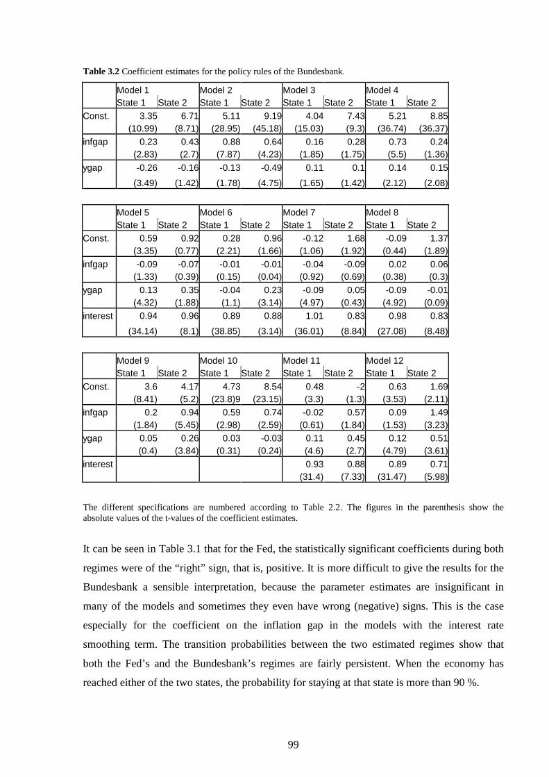
99

Table 3.2 Coeff icient estimates for the policy rules of the Bundesbank.

Model 1 Model 2 Model 3 Model 4 State 1 State 2 State 1 State 2 State 1 State 2 State 1 State 2

Const. 3.35 6.71 5.11 9.19 4.04 7.43 5.21 8.85 (10.99) (8.71) (28.95) (45.18) (15.03) (9.3) (36.74) (36.37)

infgap 0.23 0.43 0.88 0.64 0.16 0.28 0.73 0.24 (2.83) (2.7) (7.87) (4.23) (1.85) (1.75) (5.5) (1.36)

ygap -0.26 -0.16 -0.13 -0.49 0.11 0.1 0.14 0.15

(3.49) (1.42) (1.78) (4.75) (1.65) (1.42) (2.12) (2.08)

Model 5 Model 6 Model 7 Model 8 State 1 State 2 State 1 State 2 State 1 State 2 State 1 State 2

Const. 0.59 0.92 0.28 0.96 -0.12 1.68 -0.09 1.37 (3.35) (0.77) (2.21) (1.66) (1.06) (1.92) (0.44) (1.89)

infgap -0.09 -0.07 -0.01 -0.01 -0.04 -0.09 0.02 0.06 (1.33) (0.39) (0.15) (0.04) (0.92) (0.69) (0.38) (0.3)

ygap 0.13 0.35 -0.04 0.23 -0.09 0.05 -0.09 -0.01 (4.32) (1.88) (1.1) (3.14) (4.97) (0.43) (4.92) (0.09)

interest 0.94 0.96 0.89 0.88 1.01 0.83 0.98 0.83

(34.14) (8.1) (38.85) (3.14) (36.01) (8.84) (27.08) (8.48)

Model 9 Model 10 Model 11 Model 12 State 1 State 2 State 1 State 2 State 1 State 2 State 1 State 2

Const. 3.6 4.17 4.73 8.54 0.48 -2 0.63 1.69 (8.41) (5.2) (23.8)9 (23.15) (3.3) (1.3) (3.53) (2.11)

infgap 0.2 0.94 0.59 0.74 -0.02 0.57 0.09 1.49 (1.84) (5.45) (2.98) (2.59) (0.61) (1.84) (1.53) (3.23)

ygap 0.05 0.26 0.03 -0.03 0.11 0.45 0.12 0.51 (0.4) (3.84) (0.31) (0.24) (4.6) (2.7) (4.79) (3.61)

interest 0.93 0.88 0.89 0.71 (31.4) (7.33) (31.47) (5.98)

The different specifications are numbered according to Table 2.2. The figures in the parenthesis show the absolute values of the t-values of the coeff icient estimates.

It can be seen in Table 3.1 that for the Fed, the statistically significant coeff icients during both

regimes were of the “right” sign, that is, positive. It is more diff icult to give the results for the

Bundesbank a sensible interpretation, because the parameter estimates are insignificant in

many of the models and sometimes they even have wrong (negative) signs. This is the case

especially for the coeff icient on the inflation gap in the models with the interest rate

smoothing term. The transition probabiliti es between the two estimated regimes show that

both the Fed’s and the Bundesbank’s regimes are fairly persistent. When the economy has

reached either of the two states, the probabilit y for staying at that state is more than 90 %.

100

Note that the estimated transition probabiliti es 11p and 22p for both the Fed and the

Bundesbank, although high, still differ more than only negligibly from unity. Thus, neither of

the two central banks seems to have been driven by a pure “inflation nutter ” regime during

the sample period, since this kind of regime should be fully absorbing with the transition

probabiliti es very close to unity. This follows from the obvious fact that once a central bank

has committed to very strict policy against inflation, abandoning that regime would be very

costly in terms of the lost credibilit y.

Considering then the robustness of the estimation results on our alternative sets of explanatory

variables, both the timing and the parameter values of the Fed’s regimes seem to be somewhat

sensitive on the exact specification of the model, particularly on whether the specification

contains lagged interest rate term or not. The finding is in line Kozicki (1999) and Cerra et al.

(2000) who found the estimation results to be remarkably sensitive on the way the inflation

and output gaps are measured.

The estimation results for the Bundesbank seem to be even more sensitive on the specification.

As in the case of the Fed, the parameter estimates are again particularly sensitive on the

inclusion of the lagged interest rate term in the model. In the specifications with the interest

rate smoothing term, the estimates of both the constant term and the inflation gap coeff icient

get significantly lower values than in the models without the interest rate smoothing. In

addition, if the models are divided into models with and without the lagged interest rate term,

the variation in the estimation results within the two sort of specifications is greater in the case

of the Bundesbank than in the case of the Fed.

The coeff icient estimates of the inflation and output gaps reveal that the monetary policy of

the Fed clearly seems to have been switching between two regimes during our sample period.

The first of the regimes is characterized by a stronger response to the inflation gap, while a

stronger response to the output gap is associated with the second of the regimes. This finding

also seems to be robust to the model specification, although the difference between the two

regimes seems to be less clear in the specifications with the interest rate smoothing term. It is

possible to also find some differences between the two regimes of the Bundesbank, although

the differences between the regimes are not very clear. The coeff icients for both the inflation

101

and output gap of the Bundesbank tend to either get higher values or enter as significant

parameters to the model slightly more often during the regime two.

3.2 Model evaluation

There exists a set of misspecification tests available for the Markov switching models,

including the tests for remaining autocorrelation or ARCH in the residuals, a test for

misspecification of the Markovian dynamics and a test of omitted explanatory variables.

Because of both some technical diff iculties12 and the poor small sample properties of the

residual diagnostics, the model residuals were analysed less formally, by visual inspections of

the correlograms, histograms, graphs and Q-Q plots, which are provided by the MSVAR

procedure for Ox13. Overall , according to both the histograms and the Q-Q plots, the residuals

of the models for both the Fed and the Bundesbank seemed to behave fairly well i n terms of

normality, particularly when the lagged interest rate was included in the model.

For the Fed, the histograms of the residuals from the models without the lagged interest rate

term showed signs of kurtosis or skewness. The Q-Q plots also showed signs of skewness for

one of the specifications (model 5). For the Bundesbank, the histograms showed some signs of

non-normality for both the specifications with and without the lagged interest rate. The Q-Q

plots did however suggest non-normality of the residuals of the Bundesbank models.

Signs of autocorrelation were found in some of the residual series of the specifications without

the lagged interest rate term for the models of both the Fed and the Bundesbank. This finding

has to be taken into account when looking at the t-values of the parameter estimates, since the

residual autocorrelation makes the standard errors of the parameter estimates inaccurately

estimated. No signs of heteroskedasticity were found in any of the models, at least according

to the visual inspection, when the residuals were plotted against time. The problem of hetero-

skedasticity was at least partly avoided by estimating the error term variance as state-

dependent. According to the estimation results, the error term variances did indeed differ

12 The computer program used for estimating the model did not allow for calculating the test statistics. 13 For more discussion about calculating the test statistics for Markov switching models, see e.g. Sierimo (2002), p. 116.

102

considerably between the two regimes in the cases of both the Fed and the Bundesbank. In

both cases it was the regime marked as regime two during which the variance was higher.

During the sample period, the reunification of Germany at the turn of 1980’s and 1990’s

created a major break in the institutional environment, which may have contributed to our

estimation results. The robustness of the estimation results to the sample period chosen was

examined by re-estimating six of the models (models 3,4,5,6,9,10) for two sub-samples of

1970:1 – 1990:4 and 1991:1 – 1997:4. According to the results, up until the end of the 1980’s,

our previous conclusions about both the timing and the parameter values of the estimated

regimes remains largely unchanged. Apparently due to the small number of observations, the

estimation results for the latter sub-period were not plausible, however.

3.3 Regimes of the Fed

The regime of the Fed with the higher value for the coeff icient of the inflation gap is marked

as regime two in Table 2.1. It can be seen that in the models without the interest rate

smoothing term (models 1 – 4, 9 and 10) the inflation gap coeff icient always exceeds unity in

regime two but tends to remain below unity in regime one. Thus, according to the results for

the specifications without the interest rate smoothing term, the Fed seems to have followed the

so-called Taylor principle during regime two, according to which the central bank should react

to the increased inflation by increasing also the real interest rate. The estimates for the output

gap coeff icients mostly get statistically significant values in both regimes, although regime

one is characterized by higher coeff icient values.

As already noted, including the lagged interest rate as an explanatory variable to the policy

rule somewhat changes the estimation results14. The coeff icient for the lagged interest rate

itself takes fairly high and statistically significant values (in a range of 0.6 – 0.95) in both

regimes so that the Fed seems to have had fairly strong motive to smoothe its policy actions.

When the policy rule specifications with lagged interest rate are compared with the

specifications without the lagged interest rate, it can be seen that including the lagged interest

rate results in markedly lower coeff icient estimates for both inflation and output gap. Regime

14 The result of the sensitivity of the estimation results to including the lagged interest term in the equation is broadly in line with Kozicki (1999).

103

two is still associated with higher values for inflation gap coeff icient and regime one with

higher output gap coeff icient, but the result that the Fed followed the Taylor-principle during

regime two no more holds.

As noted before, a statistically significant coeff icient estimate for the output gap in a central

bank’s reaction function need not be a sign of the central bank’s willi ngness to stabili ze

output. Instead, the central bank may be interpreting the widening output gap as an indicator

of increased inflation pressure in the near future. If this really is the case here, our estimates

for the output gap coeff icient should get a higher values in the specifications with inflation

measured as realised, rather than expected inflation. This is because the public’s inflation

expectations are likely to already contain the information on the future inflation, carried by the

output gap. Comparing the specifications based on realised inflation (specifications 9 – 12)

with those based on the expected inflation (specifications 1 – 8) reveals, in fact, that the output

gap rather seems to get higher weight when inflation is measured as expected inflation. Thus,

the estimated value for the coeff icient of output gap really seems to reflect the Fed’s attempts

to stabili ze output.

3.4 Regimes of the Bundesbank

It is rather diff icult to give the estimation results for the policy rule of the Bundesbank a

sensible interpretation. In many of the specifications, the parameter estimates are no longer

significant and in addition they sometimes have wrong (negative) signs. This is especially the

case for the coeff icient of the inflation gap in the specifications with the interest rate

smoothing term. The sensitivity of the estimation results on the presence of the lagged interest

rates is also seen in the constant term. In the models without the lagged interest rate, the

constant term clearly take higher values in regime two. With the lagged interest rate present,

the results become contradictory. A closer scrutiny of the estimated coeff icient values makes

it, however, possible to somehow divide the sample period into two regimes. During regime

two the coeff icients for both the inflation and output gap tend to either get higher values than

during the regime one or at least they get statistically significant values slightly more often.

Starting with regime two, although the coeff icients of the inflation gap get considerably higher

values than the coeff icients of the output gap, even the inflation gap coeff iecients remain

below unity in every specification, thus violating the Taylor principle.

104

In the models with the lagged interest rate term, the coeff icients are not even statistically

significant in most cases. Moreover, the coeff icient on the output seems to get lower values

when the inflation is measured as expected instead of the actual inflation15. Thus, our results

support the view that by reacting to changes in output gap, the Bundesbank may only have

attempted to react to the information about the future inflation contained in the output gap.

The coeff icient estimates for the lagged interest rate of the Bundesbank in turn get values

above 0.8. All i n all , it is possible to characterize the regime two as the regime during which

the Bundesbank has operated more aggressively in resisting inflation. Whether the

Bundesbank has also been more concerned about stabili zing output during that regime,

remains an open question.

3.5 Timing of the regimes

Figures A.1 to A.12 in Appendix IIB show the filtered, smoothed and predicted probabiliti es

for the Fed, while Figures B.1 to B.12 in Appendix II B show them for the Bundesbank. The

classification of the monetary policy into different regimes makes sense only if the estimated

timing of the regime changes reported by the figures, is robust enough with respect to model

specification. As the figures suggest, this seems to be the case more for the Bundesbank than

for the Fed. Thus, one of the main findings of the study appears to be that when the estimation

results for the Fed and the Bundesbank are compared, the regime switches of the German

monetary policy seem to be easier to track, but more diff icult to interpret.

Starting with Fed, as is seen in the figures, during the sample period 1970 – 1998, the US

economy fluctuated between the two regimes with both regimes having been in force for

roughly the same length of time. The timing of the results is most robust during both the years

beginning at the turn of the eighties and at the turn of the nineties. The models with interest

rate smoothing suggest that the sample period begins driven by regime one, the Fed being

more concerned about stabili zing output than inflation. Starting around 1979, there seems to

have been a switch to regime two, which has lasted until around the mid-eighties. Because it is

regime two with the higher estimate for the coeff icient of the inflation gap, this result does not

15 During regime two, in models with inflation measured as realized inflation, the coeff icient of output gap took a statistically significant value in three cases out of four. In the eight models where inflation was measured as expected inflation, the output gap was a significant explanatory variable only twice.

105

sound surprising: At the turn of the 1970’s and 1980’s, the Fed changed its operating

procedure, which resulted in a sharp tightening of the monetary policy. The rest of the sample

period then, beginning in the latter half of the eighties and ending at the end of the nineties,

seems to be characterized by regime one again.

When we look at the models estimated without the interest rate smoothing term, our view of

the timing of the regimes changes somewhat. The sample period seems to begin as driven by

the regime one again, but then the regime turns to regime two at the middle of the 70’s. The

figures suggest that regime two seems to have lasted about ten years, ending in the latter half

of the eighties. The sample period ends dominated by regime one, as in the case of the models

with the lagged interest rate term.

For the Bundesbank, most of the time paths of the smoothed probabiliti es take roughly similar

shapes with three to four clearly observable peaks for both regimes. In addition, for all the

models, the timing of the regimes seems to be much the same at least for the first twelve years.

The first half of the 1970’s is diff icult to assign to either of the two regimes, since the

Bundesbank seems to have been wavering between the two regimes without any clear

tendency to stay at either of the states for a longer period. The figures suggest, however, that at

least the years around the first oil price shock beginning in 1973 are dominated by regime two.

The same seems to be true around the mid-eighties and at the turn of the eighties and nineties

The subperiods dominated by the regime one, in turn, take place just after the mid seventies,

around the mid eighties and at the end of the nineties.

3.6 Economic interpretation of the regimes

As previously noted, the changes in the estimated parameter values of the policy rules do not

need to have anything to do with changes in the deep parameters of the social welfare function

of the central banks. Four different sources of interpretation for our results will be discussed

instead 16.

16 There is an implicit assumption throughout the paper that the Bundesbank really did conduct autonomous monetary policy during the sample period although the DEM was adjustable with other European currencies for quite a long period. The autonomy follows from the well -known fact that the Bundesbank acted as a leader among the central banks in the EMS area.

106

1. The values of the output gaps may provide at least partial explanation for the regime

switches. It is possible that during periods with positive output gaps a central bank may

perceive the costs of highly anti-inflationary monetary policy to be lower than during

periods with an already negative output gap and vice versa. Thus, for the Fed, the

occurrence of the two regimes is compared to the concurrent values of the output gap. For

the Bundesbank this kind of comparison was however not possible because of some

technical diff iculties.17

2. The low estimates for the inflation gap coeff icient especiallu during the regime one in the

case of the Fed and during both regimes in the case of the Bundesbank may partly be due

to the low variation in inflation during those periods. It is possible that the two central

banks reacted only to relatively large changes in the rate of inflation during the sample

period, but ignored small changes. If this really was the case, then the coeff icient of the

inflation gap gets a low estimate during the periods when the variation in inflation has

been low.

3. The low value for the inflation gap coeff icient may be a sign of a period of non-

Wickselli an monetary policy. This explanation is closely related to the Taylor principle

mentioned before.

4. The estimation results will also be discussed in light of the previous literature. Goodfriend

(1995) and Judd and Rudebusch (1998) provide an interesting interpretation for the Fed’s

monetary policy since the late 1970’s. Von Hagen (1995) and Clarida et al. (1998) in turn,

discuss the monetary policy of the Bundesbank.

3.6.1. Does the state of the business cycle matter?

Beginning with the first of the possible explanations, when the output is below its potential

level, there is more room for a central bank to ease monetary policy when facing a widening

output gap, because the easing is less likely to increase inflation. By contrast, if the output is

17 This argument is analogous to discussion by Fitoussi and Creel (2002, pp. 30-31), who consider the possibilit y that the prevaili ng low level of inflation and high level of unemployment may have resulted in inertia in the monetary policy of the ECB at the time it was set up.

107

above its potential, it is more diff icult for the central bank to ease the monetary policy without

a fear of increasing inflation even if it is facing a sharp temporary decline in output growth18.

Thus, it should be expected that in the case of the Fed, the output was below its potential level

during regime one while regime two should be associated with the output above its natural

level. The hypothesis is discussed using Figure III .1 in the Appendix III , which plots the series

of our two estimates for the output gap of the US. As is seen, the US output seems to exceed

its potential level during the years 1972-74, 1978-81, 1986-91, and 1996-, while during the

rest of the time the output gap seems to get negative values. Thus, regime one (two) fairly well

seems to be associated with periods with a negative (positive) output gap. The first half of the

1970’s forms an exception, since for that period it is diff icult to say anything about the link

between the output gap and the regime switches. The identification of the policy regime

during that time was rather sensitive on the model specification. During the latter half of the

1970’s, however, the behaviour of the Fed was quite well i n accordance with the explanation

above. According to almost every graph, the Fed’s policy seems to have been driven by

regime one during that time, and the years 1974 – 1978 also seem to have been characterized

by output above its potential level.

The anti-inflationary monetary policy at the turn of the 1970’s and 1980’s could also be

understood in terms of the concurrent value of the output gap. At the end of the 1970’s, output

seems to have been above its potential and that period also corresponds to regime two. It has

to be noted, however, that the output gap already turned negative at the beginning of the

1980’s, probably just as a result of the sharp tightening of the monetary policy. Finally, even

the dominance of regime one during the most of the 1990’s fits in the above framework.

Although real growth during the period was high, output remained below its potential level

until 1996, which left room for relatively easy monetary policy without any need to worry

about inflation.

18 Clarida and Gertler (1996) made a very similar exercise when they searched for an explanation for their low estimate of the Bundesbank’s inflation gap coeff icient. Instead of output gap, they examined the possible asymmetry of the monetary policy response to the value of the inflation gap. Clarida and Gertler indeed found that the Bundesbank’s policy reacted more strongly to inflation when the inflation gap was positive. Our decision to examine the output gap rather than inflation gap is based on the fact that the diff iculties to estimating the inflation gap appears even more problematic than estimating the output gap.

108

Unfortunately, in the case of the Bundesbank, comparing the timing of the regimes with the

concurrent output gap provides a less fruitful means to interpret the results than with the US

case. The differences between the Bundesbank’s two regimes were small and neither of the

two regimes could easily be classified as a strict “ inflation nutter” regime. Moreover, as seen

in Figure III .2 in Appendix III , the two measures of the output gap deviate from each other

during the sample period. The OECD estimate of the output gap seems to “ lead” the output

gap measure based on the potential output estimate obtained by H-P filtering 1-2 years through

the whole period. Of course, the possible inaccuracies in the output gap estimates limit also

the reliabilit y of the conclusions we made in the case of the Fed.

3.6.2 Do the central banks react only to large swings of inflation?

The coeff icient of the inflation gap got remarkably low estimates during regime one in the

case of the Fed and during both of the regimes in the case of the Bundesbank19. Whether this

finding could be explained by the low variation in inflation during those periods, was

examined next. For both central banks, the sample period was divided into sub-periods that

roughly correspond to the timing of the policy regimes. Next, the standard deviations of

inflation in the US and in Germany were calculated separately for each subperiod. For the US,

the periods are 1970:1 – 1979:4, 1980:1 – 1986:4 and 1987:1 – 1997:4 and they roughly

correspond to the timing of our two estimated regimes.

The standard deviations were calculated for all four measures of inflation or inflation gap. It

appeared that the volatilit y of inflation was as its lowest (at the level of 0.31 – 0.78) during the

third of the periods, regardless of the way the inflation or inflation gap is measured. This

period actually corresponds to regime one with the lower coeff icients for the inflation gap.

Moreover, with two measures for the inflation, volatilit y was at its lowest during the second of

the periods that in turn corresponds to regime two with its higher coeff icients for the inflation

gap. On the other hand, with two out of four different measures of inflation, volatilit y was

highest during the first of the periods, which also corresponds to regime one. Hence, the

evidence is rather mixed for drawing clear conclusions about the role of the low variabilit y of

inflation (gap) in explaining the estimated low coeff icient values for the regime one.

109

During the Bundesbank’s both regimes, the coeff icient estimates for both the inflation and the

output gap get rather low values. Thus, for Germany, the volatiliti es were computed for both

inflation and output (gaps) to ascertain, whether the low variabilit y of the explanatory

variables is the reason for the low coeff icient estimates20. Standard deviations of the series

were calculated for the whole estimation period and for five subperiods of 1970:1 – 1974:4,

1975:1, 1979:4, 1980:1 – 1983:4, 1984:1 – 1990:4, 1991:1 – 1997:4, roughly corresponding to

the timing of the regimes. For the whole period, the standard deviations range from 0.9 to 1.9

for inflation and from 2.0 to 2.5 for the output gap. The two periods with more volatile

inflation were those of 1975:1 – 1979:4 and 1991:1 – 1997:4. The volatiliti es of inflation and

output seem not to have been lower in Germany than in the US during the sample period.

Thus, the low volatilit y of the explanatory variables does not seem to provide a likely

explanation for the low estimated values for the coeff icient of the reaction function.

3.6.3 Monetary policy of the Fed and the Bundesbank in the Wicksellian framework

The Wickselli an framework rests on the concept of a “natural rate of interest”21. The natural

rate of interest is determined by the supply side factors of the economy, being independent of

monetary policy. It can be defined as an equili brium rate at which the total demand equals the

natural rate of output. A deviation from the natural level of interest rate is then the ultimate

cause for the increasing inflation and the deviations from the natural level of output. The

Wickselli an analysis results in the conclusion that the monetary policy should be conducted

according to the so-called Taylor principle, that is, the nominal interest rate should be adapted

enough to also change the real rate of interest.

Woodford (2000) examines the stabili zing properties of several variants of the simple Taylor

rule in the Wickselli an framework. He uses a simple macro model to derive the necessary and

suff icient conditions for the price determinacy. Woodford found that in order to achieve price

determinacy, the policy rule should respond to both deviations of output and inflation and to

the variation of natural rate of interest. Basically, these conditions rely on the Taylor principle:

At least in the long run, the central bank should react to inflation by increasing the nominal

19 Also in two specifications for the Fed with the lagged interest rate in the rule (specifications 11 and 12) the inflation gap got remarkably low values in both regimes. 20 The low variabilit y of the explanatory variables is the explanation for the low coeff icient values if the central bank has been interested to stabili ze only large deviations of inflation and output from their equili brium values. 21 See also Blinder (1999, Ch. 2.), who uses the closely related term “neutral” monetary policy.

110

interest rate by more than the increase in the inflation rate. A suff icient condition for the

Taylor principle to hold is that the coeff icient of the inflation gap exceeds unity. Woodford

relaxes this assumption a littl e and suggests a set of necessary conditions for the price

determinacy that also include the coeff icient for the output gap and the deviations from the

equili brium real rate of interest.

Taylor (1998) and Clarida et al. (1999) provide discussion about the stabili zing properties of

the Fed’s monetary policy actions in context of the Taylor principle and the Wickselli an

framework. Taylor found that the interest rate increases of the Fed in the face of increasing

inflation during the 1960s and the 1970s were not aggressive enough to increase the real

interest rate. Too easy a monetary policy then contributed to the high inflation of the 1960s

and 1970s but beginning at the 1980s the Fed’s policy against inflation turned more

aggressive. Clarida et al. (1999) found support for Taylor’s findings, when they discussed the

values of the parameters of the monetary policy rule of the Fed in the Wickselli an framework.

For the coeff icient of expected inflation Clarida et al. yielded estimates significantly below

one that the period preceding Volcker’s appointment as the Fed chairman. Accordingly, the

authors concluded that the high and volatile inflation from the late 1960’s to the early 1980’s

may have been a result of monetary policy that did not follow the Taylor principle.

The estimation results of Clarida and Gertler (1996) and Clarida et al. (1998) cited previously,

can also be discussed within the Wickselli an framework. According to the first of the studies,

during the sample period 1974 :8 – 1993:09 the Bundesbank reacted to the widening inflation

gap by also raising the real rate of interest, thus fulfilli ng the Taylor principle. The latter of the

studies in turn suggests that the year 1979 divides the monetary policy of all three large central

banks, the Fed, the Bundesbank and the bank of Japan, into two sub-periods so that only

during the latter was their monetary policy in accordance with the Taylor principle.

In our study the Wickselli an framework was taken into account by examining whether the

parameter values of the estimated policy rules fulfil Woodford’s conditions for price

determinacy. In the case of the Fed, the results were somewhat contradictory, since signs of

Wickselli an policy were found only in the model specifications without the interest rate

smoothing term. In some cases the confidence bands for the estimated parameter values also

tended to imply borderline cases between Wickselli an and non-Wickselli an policy.

111

In the case of the Bundesbank, by contrast, the parameter values of all twelve models strongly

and consistently suggest that the Bundesbank has followed non-Wickselli an monetary policy

during both its regimes. Thus, our estimation results are in accordance with the conclusions of

Clarida et al. (1998) when it comes to the period prior 1979. The results, however, contradict

the results of Clarida et al. (1996).

3.6.4 Results in light of previous studies

It is possible also to try to interpret the estimation results by discussing them in light of some

previous studies. Goodfriend (1995) explains the Fed’s policy actions by “ inflation scares” .

Inflation scares are defined as significant long-term interest rate rises without the preceding

sharp tightening of monetary policy on the part of the Fed. When facing an inflation scare, the

Fed is, however, obliged to act by raising its policy rate, regardless of the negative effects to

the real activity, since the inflation scares tend to be self-fulfilli ng through the workers’ and

firms’ wage and price decisions. Hence, Goodfriend’s interpretation of the Fed’s policy

supports the view that the US monetary policy has been markedly forward-looking. Thus,

when interpreting the estimation results of this study, we should at least put more emphasis on

the estimation results obtained with the specifications based on expected rather than on

realized inflation.

Judd and Rudebusch (1998) tried to find out whether the Fed’s monetary policy changed when

the Fed’s chairman changed. In our study, particularly the policy rule specifications with the

interest rate smoothing term seem to imply regime switches that are somewhat in line with

changes in the Fed’s chairman. Beginning with the chairmanships of Burns (1970:1 – 1978:2)

and Greenspan (1987:3 – 1997:4), the estimation results suggest that the periods are driven by

regime one with a weaker response from the Fed to the inflation gap. Similarly, according to

Judd and Rudebusch’ study, the coeff icient for the inflation gap did not get a significant value

during the Burns’ chairmanship. Moreover, both in this study and in that by Judd and

Rudebusch, the estimates for the coeff icient of the output gap suggest that the Fed was

concerned with stabili zing output during Burns’ period. Further, our estimation results suggest

that Volcker’s period (1979:3 – 1987:2) is driven by regime two. Likewise, according to Judd

and Rudebusch’s characterization the Fed did not respond to the level of output gap during

that time, although it seemed to have reacted to changes in it. On the other hand, the estimates

112

of the coeff icients of the inflation gap are larger in our study compared with the estimate of

about 0.5 by Judd and Rudebusch.

Von Hagen (1995) in turn, attempts to explain the Bundesbank’s actions during the Bretton-

Woods era. He suggests that the Bundesbank’s goal was the targeting of inflation and

monetary growth at the same time. According to von Hagen, the Bundesbank’s primary goal

has been to stabili ze long-term inflation. Long-term inflation is measured as the trend-rate of

change of the equili brium price level, not the observed actual inflation or sudden discrete

shifts in the price level. The equili brium price level in turn is defined as the price level that

clears the money market. Von Hagen highlights the importance of reputation building for the

Bundesbank throughout the whole sample period. Because of this reputation-building motive,

the Bundesbank has occasionally even targeted price level instead of inflation. According to

von Hagen, the Bundesbank has adopted the price level target whenever the German economy

has faced a rapid temporary shift in price level. The motivation for this was the fear that

private agents would have diff iculties in separating a temporary shift in the price level from

increased inflation. This kind of misinterpretation would then have led to increased inflation

expectations and hence to cost-push inflation. Thus, von Hagen’s conclusions partly account

for the relatively low explanatory power of the inflation gap in our estimations, if the

Bundesbank really was targeting rather the equili brium price level instead of actual inflation

that we have focused.

Our estimated timing of regime switches also seems to be in line with the interpretations of

von Hagen. According to him it is possible to identify three periods during the post Bretton

Woods era with an initial upward jump in the equili brium price level. The jumps were

followed by the marked decline in prices that comes with a severe recession. The timing of

these jumps and declines coincides quite accurately with the periods of regime two, when the

Bundesbank seemed to be at least somewhat more concerned of stabili zing both inflation and

output. The first jump took place after the first oil -price shock in 1974-5, the second after the

second oil -price shock and the appreciation of the US dollar in 1980-2 and the last one after

German reunification. On the other hand, our estimates of the transition probabiliti es between

the regimes contradict von Hagen’s interpretations. If the Bundesbank really had pursued a

price level target, it would have been expected to almost certainly stay at that regime once it

has been reached. My estimates for the probabiliti es of the shifts between the regimes,

however, were considerably above zero.

113

4. CONCLUSIONS

In this paper the monetary policy rules of the Federal Reserve and the Bundesbank were

studied using Markov Regime switching models. Because of the well -known problems with

the correct way to measure inflation and output gaps, several alternative data sets and

specifications were used in the estimations. It was concluded, firstly, that during the post

Bretton-Woods era, there seems to have been several sudden regime switches in the

parameters of the reaction functions of both the Federal Reserve and the German Bundesbank.

Secondly, the estimation results of the coeff icients of the policy rule and the timing of the

regimes turned out to be somewhat sensitive on the exact model specification concerning the

way inflation and the output gap are measured and particularly on whether the specification

contains an interest rate smoothing term or not. It was found that the regime switches of the

German monetary policy are be easier to track, but more diff icult to interpret than the US

regimes.

The sensitivity of the coeff icient estimates to the model specification is broadly in line with

some previous studies by e.g. Orphanides (1997), Kozicki (1999) and Cerra et al. (2000) who,

using linear models, concluded that the Taylor rule estimates may be sensitive to the exact

specification of the rule or on the way the inflation and output gaps are defined. As Kozicki

(1999) points out, however, although the sensitivity of the Taylor rules on minor variations

made to their assumptions limits their role as a tool for real-time monetary policy decisions,

the rules can still be of valuable use. For instance, the Taylor-type rules can still serve as

valuable components in forecasting models, since many of the real-world problems related to

the rules disappear in the modelli ng frameworks, which already are extensively simpli fied.

Nevertheless, since the Markov switching models seem to fit the data relatively well,

irrespective of the exact specification, the stabilit y of the feedback rules of both Fed and

Bundesbank during the sample period may well be called into question. The two regimes of

the Federal Reserve were identified as a regime with the stronger response to the inflation and

a regime in which the Fed was more interested in stabili zing output. The economic

interpretation for the regimes was detected by comparing, for instance, the timing of the

regimes with the concurrent value of the output gap during the sample period and by trying to

find evidence about possible price indeterminacy in the parameter values of the policy rules. It

was found that the Fed reacted to inflationary pressures more strongly during periods with

114

output above its potential. Some evidence was also found that our estimated regime changes to

some extent go hand in hand with the changes in the holder of the Fed’s chairmanship. The

possible existence of price indeterminacy in turn remains an open question since the

estimation results did not permit firm conclusions to be drawn about this question.

In the case of the German Bundesbank, it was not possible to make a clear distinction between

the regimes to a regime with more emphasis put on resisting inflation and a regime with more

emphasis put on stabili zing output. Instead, during the first of the regimes, the coeff icient

values for neither inflation nor output gap turned out to be statistically significant. The other

regime in turn was characterized by statistically significant, but still rather low coeff icient

values for both the inflation and the output gap, at least in some model specifications. Because

the output gap seemed to lose its explanatory power when inflation was measured by expected

inflation, the higher estimate for the output gap coeff icient may, however, only reflect the

Bundesbank’s reaction to the information content of the future inflation of the output gap,

rather than real concern of stabili zing output. Hence, one of the two regimes may be

considered a regime when the Bundesbank was more active in resisting inflation. The values

for the inflation gap, however, remained low enough during both regimes to suggest price

indeterminacy for the whole sample period, if the Wickselli an framework is valid.

Our results turned out to be at least partly in line with von Hagen’s (1995) interpretation of

theBundesbank’s monetary policy. That is, although the Bundesbank has mainly targeted

long-run inflation instead of monetary aggregates, it has occasionally adopted temporary price

level targeting when facing sudden discrete shifts in the actual price level. The estimated

timing of regime two coincides fairly well with the periods of price level targeting proposed

by von Hagen. Some further understanding of the empirical findings was also found by

comparing the timing of the regimes with the institutional changes during the sample period.

115

REFERENCES

Ang, A. – Bekaert, G. (1998)

Regime Switches in Interest Rates

NBER Working Paper 6508

Blinder, A. S. (1999)

Central Banking in Theory and Practice

The MIT Press. Cambridge

Cerra, V. – Saxena, S. C. (2000)

Alternative Methods of Estimating Potential Output and the Output Gap: An

application to Sweden

IMF Working Paper 59 /2000.

Clarida, R. – Gali , J. – Gertler, M. (1999)

Monetary Policy Rules and Macroeconomic Stabili ty: Evidence and Some Theory

Universitat, Pompeu Fabra, Economic Working Papers n:o 350.

Clarida, R. – Gali , J. – Gertler, M. (1998)

Monetary policy rules in practice. Some international evidence.

European Economic Review 42 (1998).

Clarida, R. – Gertler, M. (1996)

How the Bundesbank Conducts Monetary Policy

NBER Working Paper 5581. Cambridge.

Evans, C. L. (1998)

Real Time Taylor Rules and the Federal Funds Futures Market

Economic Perspectives, Federal Reserve Bank of Chicago, Third Quarter 1998.

Fitoussi, J-P. – Creel, J. (2002)

How To Reform the European Central Bank

Centre for European Reform, 2002.

116

Goodfriend, M. (1995)

Acquir ing and Maintaining Credibili ty for Low Inflation: The US Experience.

in Inflation Targets, edited by Leiderman, L. – Svensson, L. E. O.

CEPR, 1995.

Judd, J. P. – Rudebusch, G. D. (1998)

Taylor ’s Rule and the Fed: 1970-1997

Federal Reserve Bank of San Fransisco Economic Review, 3/1998.

http://www.frbsf.org/econrsrch/econrev/index.1998.html

Kajanoja, L. (2001)

Essays on Currency Cr ises and Exchange Rate Expectations

University of Helsinki. Research Reports No. 88:2001.

Kozicki, S. (1999)

How Useful are Taylor Rules for M onetary Policy?

Federal Reserve Bank of Kansas City Economic Review 2/1999.

Linde, J. (2000)

Testing for the Lucas Cr itique: A Quantitative Investigation

Stockholm School of Economics Working Paper Series 311 / 2000.

Orphanides, A. (1997)

Monetary Policy Rules with Real-Time Data.

Board of Governors of the Federal Reserve System, December.

Peersman, G. – Smets, F. (1998)

Uncertainty and the Taylor r ule in a simple model of the euro-area economy

Federal Reserve Bank of San Fransisco, Proceedings 266.

Runkle, D. E.

Revisionist History: How Data Revisions Distor t Economic Policy Research

Federal Reserve Bank of Minneapolis Quarterly Review Vol. 22, No. 4.

117

Sack, B. (2000)

Does the Fed act gradually? A VAR analysis

Journal of Monetary Economics 46 (2000) 229 – 256.

Sierimo, C. (2002)

Testing the Eff icient Market Hypothesis of the Helsinki Stock Exchange – Fur ther

empir ical evidence based on nonlinear models

University of Helsinki. Research Reports No. 91:2002.

Sill , K. – Wrase, J. (1999)

Exchange Rates and Monetary Policy Regimes in Canada and the U.S.

Federal Reserve Bank of Philadelphia Working Paper no 99-13.

Taylor, J. B. (1993)

The robustness and eff iciency of monetary policy rules as guidelines for interest rate

sett ing by the European Central Bank.

Institute For International Economic Studies Seminar Paper No. 649.

Taylor, J. B. (1998)

An Histor ical Analysis of Monetary Policy Rules

NBER Working Paper 6768. Cambridge.

Von Hagen, J. (1995)

Inflation and Monetary Targeting in Germany

in Inflation Targets, edited by Leiderman, L. – Svensson, L. E. O.

CEPR,1995. Woodford, M. (2000)

A Neo-Wickselli an Framework for the Analysis of Monetary Policy

Manuscript. Princeton University.

(Available at http://www.princeton.edu/~ woodford/)

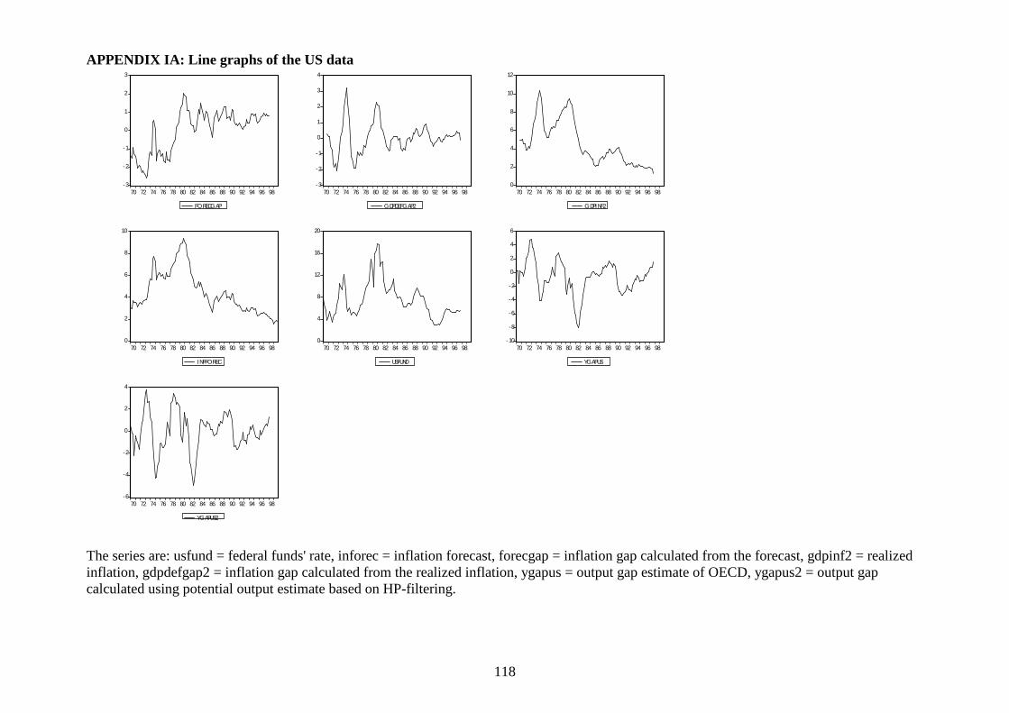
118

APPENDIX IA: L ine graphs of the US data The series are: usfund = federal funds' rate, inforec = inflation forecast, forecgap = inflation gap calculated from the forecast, gdpinf2 = realized inflation, gdpdefgap2 = inflation gap calculated from the realized inflation, ygapus = output gap estimate of OECD, ygapus2 = output gap calculated using potential output estimate based on HP-filtering.

-3

-2

-1

0

1

2

3

70 72 74 76 78 80 82 84 86 88 90 92 94 96 98

FORECGAP

-3

-2

-1

0

1

2

3

4

70 72 74 76 78 80 82 84 86 88 90 92 94 96 98

GDPDEFGAP2

0

2

4

6

8

10

12

70 72 74 76 78 80 82 84 86 88 90 92 94 96 98

GDPINF2

0

2

4

6

8

10

70 72 74 76 78 80 82 84 86 88 90 92 94 96 98

I NFFOREC

0

4

8

12

16

20

70 72 74 76 78 80 82 84 86 88 90 92 94 96 98

USFUND

-10

-8

-6

-4

-2

0

2

4

6

70 72 74 76 78 80 82 84 86 88 90 92 94 96 98

YGAPUS

-6

-4

-2

0

2

4

70 72 74 76 78 80 82 84 86 88 90 92 94 96 98

YGAPUS2

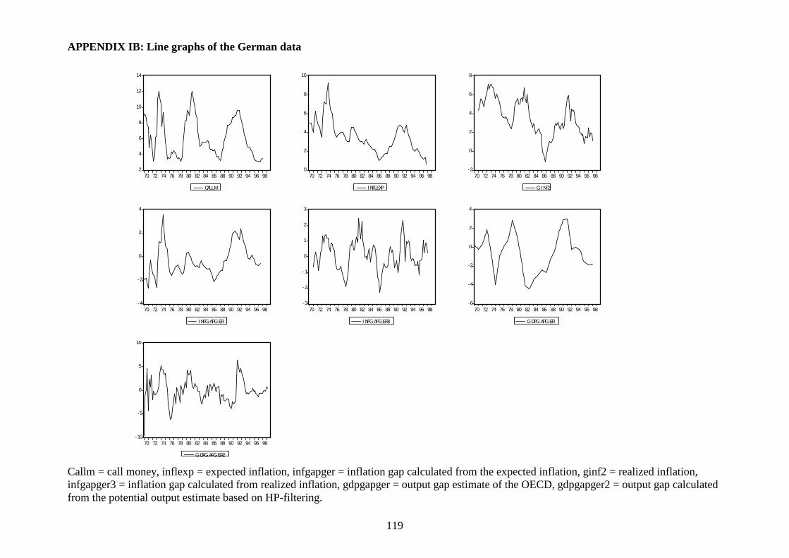
119

APPENDIX IB: L ine graphs of the German data Callm = call money, inflexp = expected inflation, infgapger = inflation gap calculated from the expected inflation, ginf2 = realized inflation, infgapger3 = inflation gap calculated from realized inflation, gdpgapger = output gap estimate of the OECD, gdpgapger2 = output gap calculated from the potential output estimate based on HP-filtering.

2

4

6

8

10

12

14

70 72 74 76 78 80 82 84 86 88 90 92 94 96 98

CALLM

0

2

4

6

8

10

70 72 74 76 78 80 82 84 86 88 90 92 94 96 98

I NFLEXP

-2

0

2

4

6

8

70 72 74 76 78 80 82 84 86 88 90 92 94 96 98

GI NF2

-4

-2

0

2

4

70 72 74 76 78 80 82 84 86 88 90 92 94 96 98

I NFGAPGER

-3

-2

-1

0

1

2

3

70 72 74 76 78 80 82 84 86 88 90 92 94 96 98

I NFGAPGER3

-6

-4

-2

0

2

4

70 72 74 76 78 80 82 84 86 88 90 92 94 96 98

GDPGAPGER

-10

-5

0

5

10

70 72 74 76 78 80 82 84 86 88 90 92 94 96 98

GDPGAPGER2

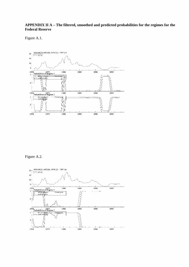
120

APPENDIX II A – The fil tered, smoothed and predicted probabili ties for the regimes for the Federal Reserve

Figure A.1.

Figure A.2.

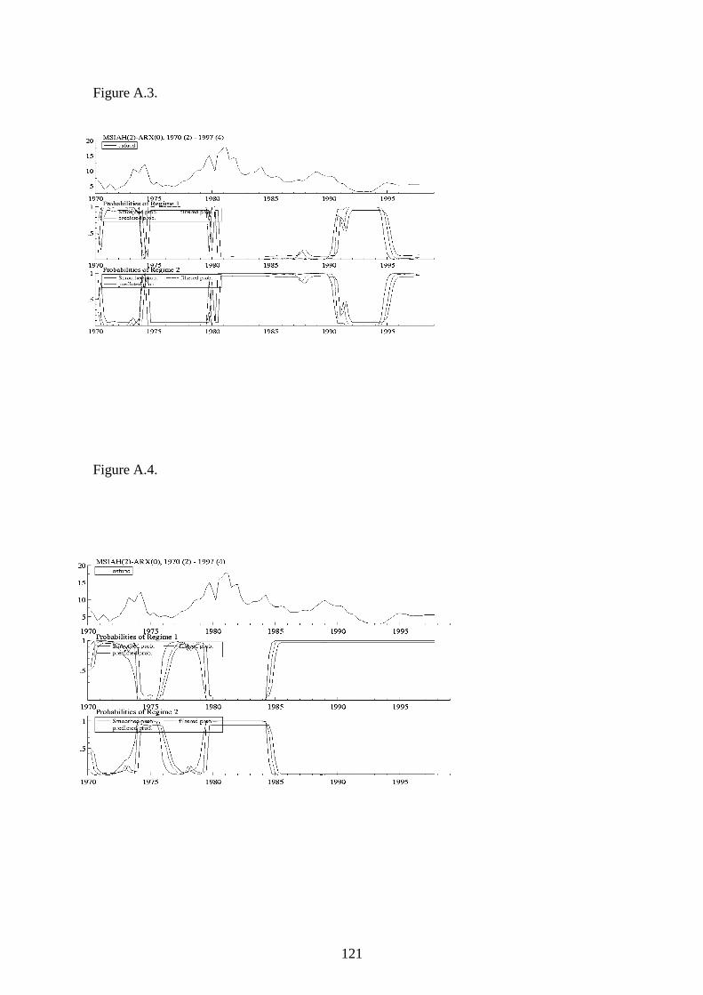
121

Figure A.3.

Figure A.4.

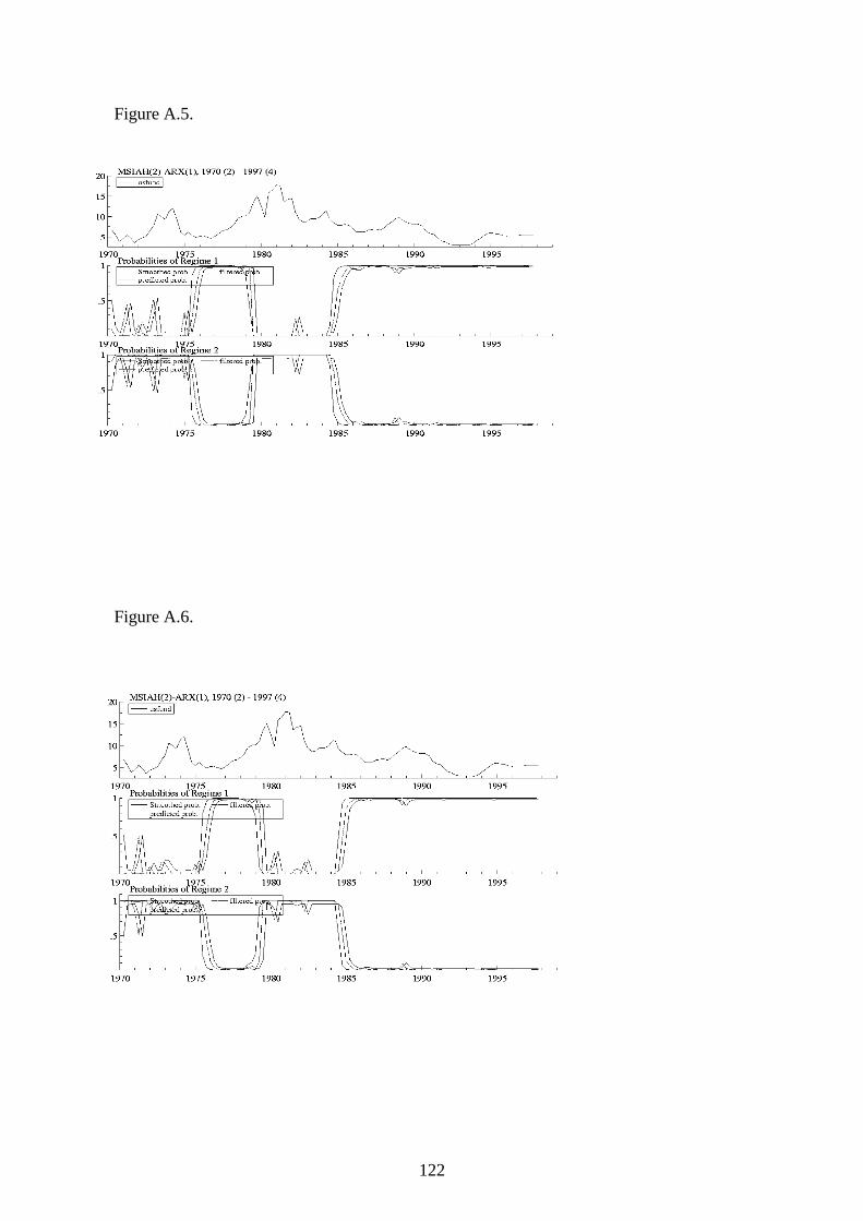
122

Figure A.5.

Figure A.6.

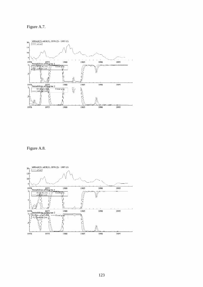
123

Figure A.7.

Figure A.8.

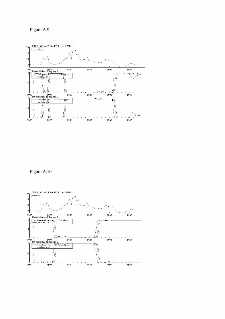
124

Figure A.9.

Figure A.10.

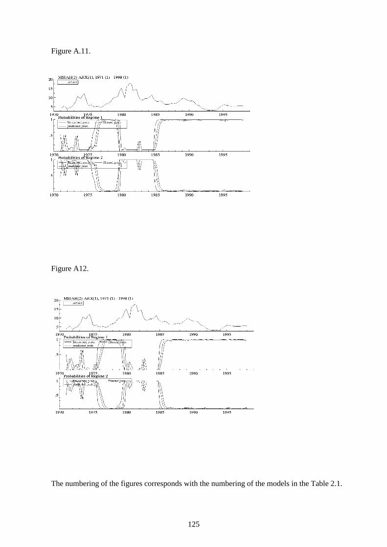
125

Figure A.11.

Figure A12.

The numbering of the figures corresponds with the numbering of the models in the Table 2.1.

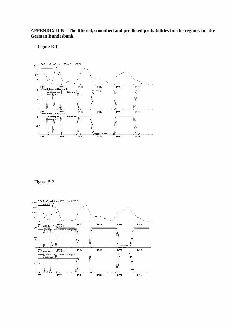
126

APPENDIX II B – The fil tered, smoothed and predicted probabili ties for the regimes for the German Bundesbank

Figure B.1.

Figure B.2.

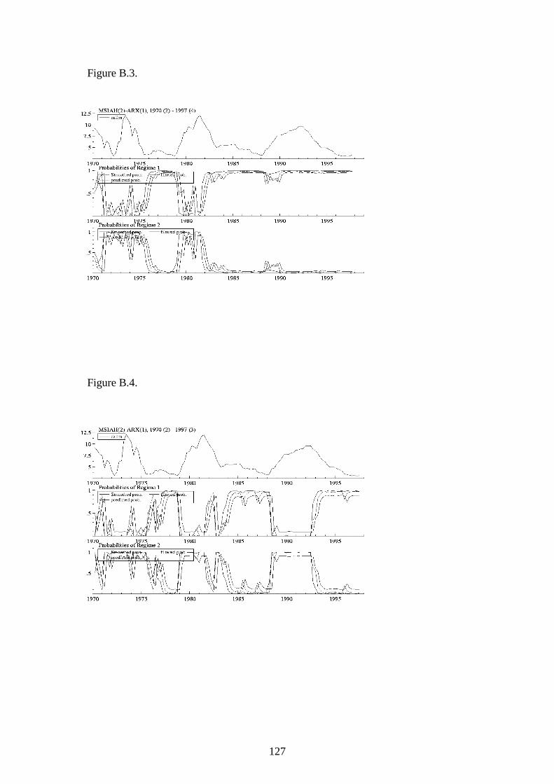
127

Figure B.3.

Figure B.4.

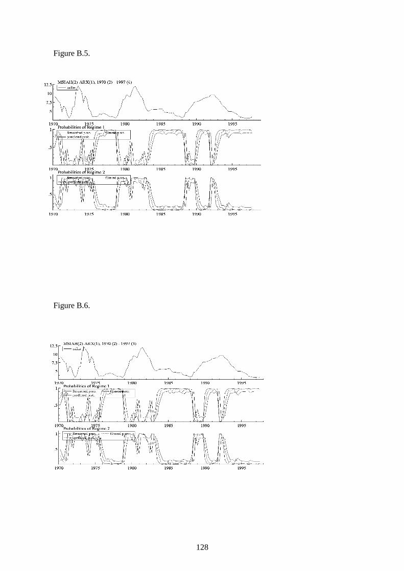
128

Figure B.5.

Figure B.6.

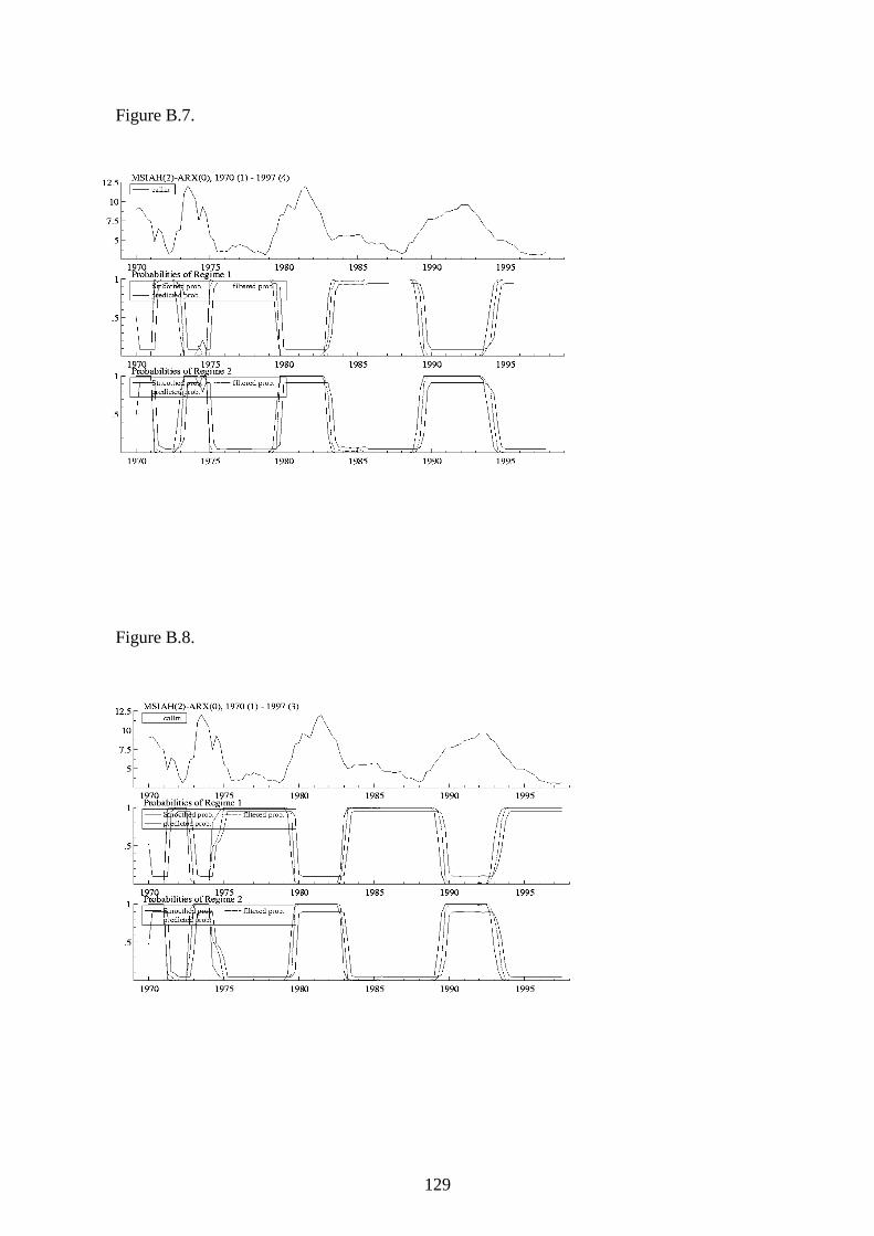
129

Figure B.7.

Figure B.8.

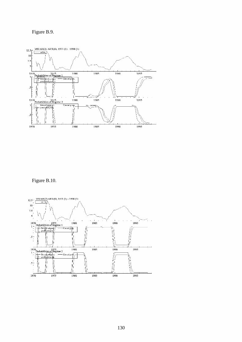
130

Figure B.9.

Figure B.10.

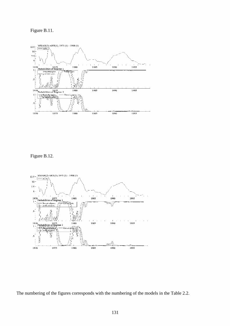
131

Figure B.11.

Figure B.12.

The numbering of the figures corresponds with the numbering of the models in the Table 2.2.

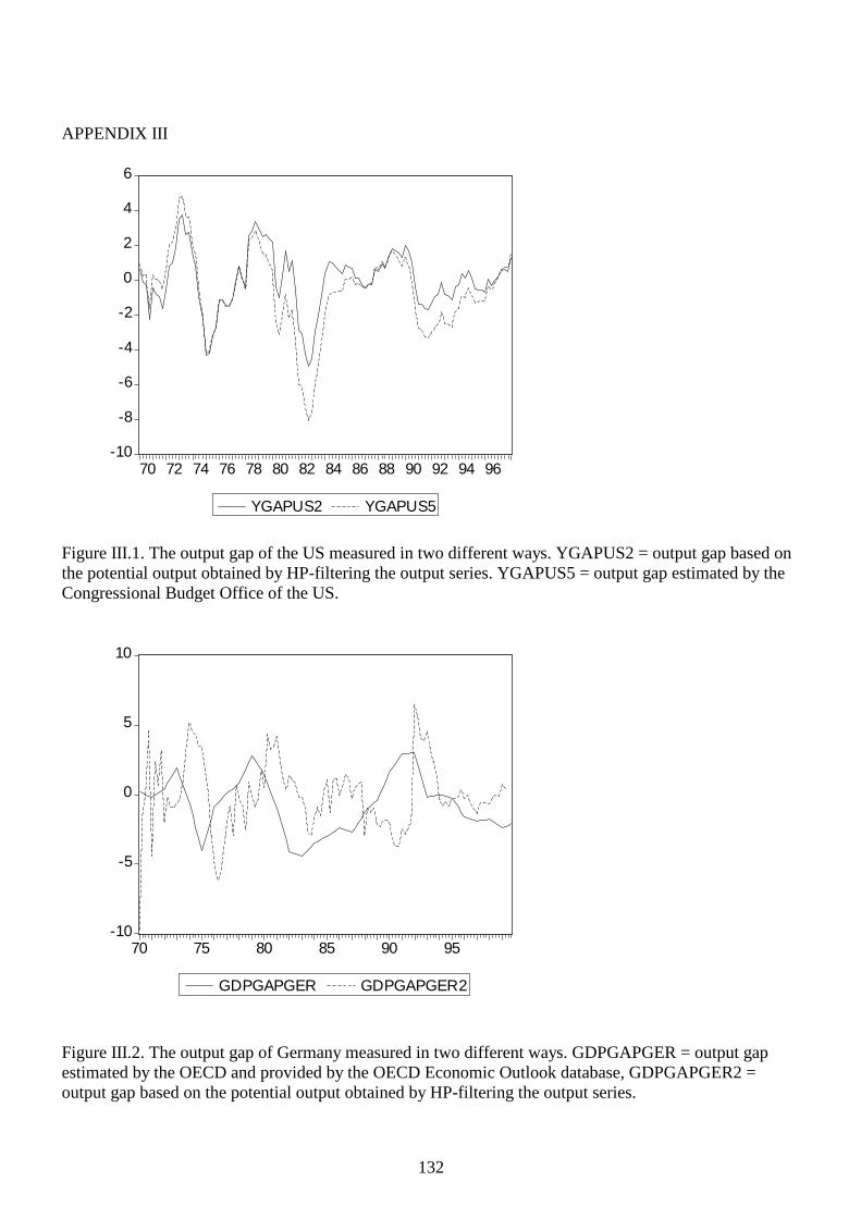
132

APPENDIX III Figure III .1. The output gap of the US measured in two different ways. YGAPUS2 = output gap based on the potential output obtained by HP-filtering the output series. YGAPUS5 = output gap estimated by the Congressional Budget Off ice of the US. Figure III .2. The output gap of Germany measured in two different ways. GDPGAPGER = output gap estimated by the OECD and provided by the OECD Economic Outlook database, GDPGAPGER2 = output gap based on the potential output obtained by HP-filtering the output series.

-10

-5

0

5

10

70 75 80 85 90 95

GDPGAPGER GDPGAPGER2

-10

-8

-6

-4

-2

0

2

4

6

70 72 74 76 78 80 82 84 86 88 90 92 94 96

YGAPUS2 YGAPUS5

133

CHAPTER 4

SHOULD THE ECB ADOPT AN EXPLICIT EXCHANGE RATE TARGET? ABSTRACT This paper uses a a structural, quantitative macro model to investigate, whether the

ECB should introduce the stabili zation of the real exchange rate of the euro as one of

the goals of its monetary policy. The problem is considered from the perspectives of

both the whole monetary union and a single member state with a national economy

more open than the union economy on average. According to the results, the member

state would benefit from exchange rate stabili zing more than the rest of the union. It

appears, however, that the asymmetries of the external shocks facing the economies

may be a more important factor behind the greater volatilit y of the inflation and

output of the member state than the structural differences.

KEY WORDS: Euro area, monetary policy rules, optimal currency areas.

JEL Classification: E32, E52, E58, F42

134

Contents 1. INTRODUCTION 135 2. THEORETICAL MODEL 139 2.1. The structure of the model 139 2.2. Solving the model 145 2.3. Calibrating and assessing the plausibilit y of the model 147 3. STOCHASTIC ANALYSIS 153 3.1. Calculation of the exogenous shocks 153 3.2. Simulations 156 3.2.1. The Union 156 3.2.2 The member state 161 3.2.3. The role of the time series properties of the shocks 166 4. CONCLUSIONS 169 REFERENCES 170 APPENDIX I The calculation of the unconditional var iances 173 of inflation and output APPENDIX II The impulse responses of the deterministic analysis 174 APPENDIX III The calculation of the unconditional var iances of 177

inflation and output

135

1. INTRODUCTION

Since the adoption of the euro, economists have been discussing whether the

stabili zation of the real exchange rate of the euro should be one of the goals of the

ECB’s monetary policy. The opponents to exchange rate interventions stress that the

primary goal of the ECB is to pursue price stabil ity, not to target the exchange rate of

the euro. On the other hand, if the fluctuations of the euro eventually pass through to

consumer prices, this will make it more diff icult to reach the inflation target.

The problem of whether the ECB should pay attention to stabili zing the exchange rate

of the euro is also a part of the discussion whether the euro area can be considered as

an optimal currency area. Because of the asymmetries in both the monetary

transmission mechanisms and in the business cycle pattern between the member

states, the same monetary policy does not necessarily suit all member states. For

example, there are considerable differences in the degree of openness of the member

states, measured as the share of foreign trade with countries outside the union.

Moreover, the exogenous shocks to aggregate demand and productivity do not hit the

single member economies symmetrically. Still t he ECB has to target only the union

wide averages of these variables.

In short, the research problem of this study is to investigate with a structural,

quantitative macro model, whether the ECB should include the real exchange rate as a

variable in its reaction function. The problem is considered both from the perspective

of the whole monetary union and from that of a single member state with a national

economy differing from the averages of the whole union both in its degree of

openness and with regard to its business cycle pattern. Another goal of the study is to

examine whether the union’s one-size-fits-all monetary policy can create significant

welfare losses because of increased deviations of inflation and output in some of the

EMU member states.

The research method of the study is to specify a quantitative, calibrated macromodel

that is consistent with both economic theory and data. The macro model is a small

“New Keynesian” model consisting of a simple monetary policy rule and equations

136

covering the essential features of both a large monetary union and a small member

state of the union. After the model has been solved, it is simulated under different

assumptions concerning the weight that is placed on stabili zing the exchange rate in

the central bank’s policy rule equation of the model. Whether increasing this weight

improves or impairs the macroeconomic performance of either the union as a whole

or its small member state, is then discussed by calculating the unconditional variances

of the inflation and output from the simulated series.

The importance of exchange rate shocks for the economic stabilit y of the EMU area

depends on its openness against the rest of the world. Peersman and Smets (1998), for

instance, argue in favour of considering the euro area as a closed economy like the US

and Japan, since the ratio of exports to the euro area-wide GDP is only about 14%. On

the other hand, some researchers have argued that the relatively low degree of

openness of the euro area does not necessarily imply an insignificant role for the

exchange rate. Mayes and Virén (1998), for instance, estimate monetary condition

indexes for groups of EMS countries. The results suggest that the significance of the

exchange rate channel for the transmission of monetary policy to both inflation and

real variables may be much larger in the euro area than could be concluded from the

volume of its foreign trade. The authors conclude that the transmission mechanism of

the exchange rate changes is not based solely on foreign trade but is a more

complicated process. The tentative results of Ranki (2001) also suggest that the

degree of pass-through may be much larger than would be expected in light of the

openness of the euro area.

Previous theoretical analyses on including a direct exchange rate target in the

monetary policy rule are provided by Ball (1998), Taylor (1999) and Svensson

(1998)1. Each of the studies approach the problem from slightly different viewpoint

but a common feature of all these studies is that the central bank policy rule is

assumed to be of the form

(1.1.) 10 −+++= tttttt eeyi λλβαπ ,

1 For a discussion of these papers, see also Taylor (2001).

137

where tπ =inflation, ty = output, te = real exchange rate and α , β , 0λ and 1λ are

parameters.

Ball uses a small macromodel to argue that in an open economy the central bank

should take the exchange rate into account in its policy by including the monetary

condition index (MCI), that is, a weighted average of the interest rate and the

exchange rate, into its reaction function. For the parameter 0λ Ball 's study implied an

optimal value of –0.37 and for 1λ a value of 0.17. The alternative policy rule

considered in Ball ’s study for comparison, pure inflation targeting, would instead

create large fluctuations in exchange rate and output.

Taylor (1999) in turn, simulates ECB interest rate rules in a dynamic stochastic

multicountry model for seven large countries. In the study the euro area was modelled

by assuming fixed exchange rates between Germany, France and Italy and a single

short term interest rate. When the performance of the original Taylor rule was

compared with that of a rule that also contained the nominal euro/USD exchange rate

as an argument, with 0λ = –0.25 and 1λ = 0.15, neither of the rules strictly dominated

the other. Instead, for some countries (France and Italy) the policy rule with the

exchange rate target led to better performance, while for Germany, this policy rule

implied poorer performance.

Svensson (1998) compared several variants of inflation targeting in an open economy

setting. When a policy rule of Equation (1.1) was considered, Svensson assumed

values 0λ = -0.45 and 1λ = 0.45. Analysing the optimal monetary policy responses to

many different shocks the author concluded that flexible CPI targeting stands out as

successful in limiti ng the variabilit y of CPI inflation, output gap and real exchange

rate.

In light of the three studies referred to above, the exchange rate should not play a very

important role in the monetary policy rules of even open economies. Adopting an

exchange rate target implied only small reductions in the volatiliti es of inflation and

output, although some of the models assumed rather large values for 0λ and 1λ . In

138

Svensson’s study, including the exchange rate in the policy rule actually seemed to

imply a slight increase in the volatilit y of output2.

The viewpoint of a single small member state on the optimal policy rule of a

monetary union is actually part of the discussion of the optimal currency areas

(henceforth, OCA). Whether the euro area can be considered an optimal currency area

or not is discussed in Bayoumi and Eichengreen (1992) and Dornbusch et al. (1998).

Bayoumi and Eichengreen discuss the symmetry of the structural shocks in the EC

area by estimating a set of structural VAR models to the 11 EC countries to identify

the demand and supply shocks hitting these economies. The authors conclude that

only the core countries of the EC experienced shocks with roughly the same

magnitude and cohesion as the US regions. Particularly the supply shocks hitting the

EC periphery tend to be both larger and less correlated with the shocks hitting the

neighbouring countries. Thus, the results suggested that operating a monetary union

may be more diff icult in the euro area than in the US.

Dornbusch et al. (1998) provide a survey of the symmetry of the monetary

transmission mechanism in the EMU area. The authors conclude that, due to the

differences in the financial systems, the wage-price processes and also in the degree

of openness of the EMU countries, the monetary processes differ widely among the

member states. Because of the already ongoing restructuring of the financial processes

and the adaptation of the labour markets of the member states to the changing

environment, the transmission mechanisms in the member states are however, li kely

to converge.3

2 The intuition behind this result is based on the indirect effect of the exchange rate on the interest rate that was built i nto the models by assuming rational expectations and some inertia. 3 Schelkle (2001) provides an alternative standpoint for the whole OCA literature. If the exchange rates no more reflect only economic fundamentals, but are more or less driven by (rational or irrational) bubbles, the exchange rate adjustment no longer provides a shelter from economic shocks. Accordingly, the presence of asymmetric shocks is no more an acceptable argument against monetary unification, and eliminating the exchange rate instabilit y becomes rather a benefit than a cost.

139

2. THEORETICAL MODEL

2.1. Structure of the model

From the methodological point of view, the study at hand represents an approach that

Taylor (2001, p. 263) calls “new normative macroeconomic research” . This approach

includes building a macroeconomic model containing a monetary policy rule, solving

the model numerically, examining the stochastic behaviour of the model variables and

choosing the monetary policy rule with the most satisfactory performance. Further, as

the macroeconomic model of this study assumes nominal rigidities, it is an example of

what Clarida et al. (1999) call “New Keynesian models” . It is typical for the New

Keynesian models that they closely resemble the traditional ISLM models, while they

still are derived from the behaviour of optimising agents4. As McCallum and Nelson

(1997) have demonstrated, the models correspond to a linear reduced form of fully-

optimising general equili brium model. A typical New Keynesian model consists of a

Taylor type monetary policy rule, an IS-curve type relation and equation(s) describing

the supply side of the economy. The model may also include an LM curve equation

and in an open economy setting the model is often supplemented by an uncovered

interest parity condition for determining the exchange rate.

Our model is built from a single country macro model by Batini and Haldane (1998)

to cover two economies, that is, the monetary union as a whole and a single member

state. (For convenience, the single member state is henceforth referred to as simply

“member state”). More formally, the model is a linear difference equation system of

ten equations, so that Equations (2.1) – (2.6) below characterize the whole monetary

union, while Equations (2.7) – (2.10) describe solely the economy of the member

state. The equations characterizing the whole union follow Batini’s and Haldane’s

model very closely, whereas the rest of the equations describing the small member

state form the “new” part of the model. Note that there is only one-way feedback

between the member state and the union: The member state takes the interest rates as

given and a relatively large share of its foreign trade is assumed to consist of intra-

4 Recent surveys of these “New Keynesian” models are provided by Clarida et al. (1999) and Taylor (2001).

140

union trade. The member state, however, is assumed to be so small relative to the

union that the union’s variables are unaffected by the performance of the economy of

the single country.

The model implies stickiness to consumer prices, and hence some persistence to

consumer price inflation. In addition, the model is forward-looking in nature and the

expectations are assumed to be rational. The forward-looking features of the model

appear in many forms. Firstly, in the policy rule the central bank reacts to anticipated

inflation. Secondly, the IS equation may be interpreted as a linearised Euler equation,

where the present consumption is affected by the expected marginal utilit y from the

consumption of the next period. Thirdly, in the uncovered interest rate parity equation

the nominal exchange rate adjusts according to the expected future paths of the

domestic and foreign short-term interest rates. Finally, in the wage contracting

equation the workers set their wage demand partly according to the expected wage

level of the future wage contracts.

141

The macro model

The monetary union

(2.1) [ ] )()()1( *3

*2

*11

*1 ttttttttt qqyyErrr −+−+−+−+= +− θθππθγγ

(2.2) [ ] ytttttttt qryEyyy εαααα ++++=− +− )()( 431211*

(2.3.) etf

ttttt iieEe ε++−= + )( 1

(2.4) [ ]12/1 −+= ttdt wwp

(2.5) [ ] [ ] wttttttt yywwEw εχχχ +−+−+= −+ )()1()( *11010

(2.6) 1)1( −−+= tdt

ct epp φφ

The small country

(2.7) [ ] mytt

mt

mt

mtt

mt

mt

mt yqryEyyy εβββββ +++++=− +− )()()( 5431211

*

(2.8) [ ]mt

mt

mdt wwp 12/1 −+=

(2.9) [ ] [ ] mwt

mt

mt

mt

mtt

mt yywwEw εψψψ +−+−+= −+ )()1()( *

11010

(2.10) 1)1( −−−++= tdt

mdt

mct eppp ϑκϑκ

All variables, except interest rates, are in logarithms. Inflation variables of both the

union and the single country, tπ and mtπ , are defined as consumer price inflation.

That is, ct

ctt pp 1−−≡π and mc

tmct

mt pp 1−−≡π , where c

tp and mctp are the price levels

of the consumption goods of the union and the member state. The nominal exchange

rate ( te ) is defined as the domestic price of foreign currency. Accordingly, the real

exchange rates of the union and the member state are defined as ct

cfttt ppeq −+=

142

and mct

cftt

mt ppeq −+= where cf

tp is the price level of the consumption goods

outside the union that is normalized to zero.5

Equation (2.1) represents the ECB’s monetary policy rule. It is assumed that while the

ECB’s policy instrument is actually the nominal interest rate, ti , it tries to adjust the

ex-ante real rate of interest ( 1+−≡ tttt Eir π ) of the whole union6 through its forecast

of the future inflation7. The policy rule is a variant of the Taylor rule so that the ECB

is assumed to respond to deviations of the expected inflation and output from their

desired levels, that is, *1 ππ −+ttE and *

tt yy − . The Taylor rule type policy rule with

inflation and output gaps as central bank’s objectives may also be motivated

theoretically, as Woodford (1999) shows8. The desired levels of the output *ty , are

implicitl y assumed to be the natural rate of output so that there is no Barro-Gordon

bias built i nto the model. In addition to the inflation and output gaps, the ECB is

assumed to react to deviations of the real exchange rate from its target ( *qqt − )9.

The right hand side of the policy rule equation also includes the lagged real interest

rate, which reflects the central bank’s urge to smooth its interest rate changes10. Such

an interest rate smoothing element has become a mainstream assumption in the

literature and it can be motivated for instance by central banks’ attempt to stabili ze

financial markets. Alternatively, the sluggishness in the interest rate changes can also

be interpreted as reflecting central banks’ caution in the face of the uncertain

information on which the central banks have to build their decisions.

5 The variables of the single member state are distinguished from the union variables by superscript m. 6 Accordingly, the real interest rate of the single member state is given by 1+−≡ t

mtt

mt Eir π .

7 According to the deterministic analysis, the results were not sensitive on whether the variable in the left hand side of the equation is the nominal or the real interest rate. 8 With a simple optimising model Woodford shows that it is possible to motivate a quadratic loss function with inflation and output gap as arguments as a second-order Taylor-series approximation to the expected utilit y of the economy’s representative household. Some of the assumptions of Woodford’s model, regarding eg the definition of the output gap, are somewhat special so that some minor quali fications would actually be needed to justify the stabili zation goals of the Taylor rule using Woodford’s model. For instance, the natural rate of output should be defined as an equili brium level that is obtained under perfectly flexible prices, and which varies as a response to the shocks the economy is facing. 9 The exchange rate could be defined e.g. as the trade-weighted exchange rate or the exchange rate between the Euro and the USD. 10 See e.g. Kozicki (1999), p. 8.

143

Equation (2.2) represents the IS curve of the economy, relating the deviation of the

real output, ty from its potential level *ty , to the ex ante real interest rate and the real

exchange rate as well as to the lagged and lead term of the output ( 0, 43 >αα ). The

right hand side of the equation contains both a lagged and a lead term of output. This

is a novel feature compared to the traditional specification of the IS curve with the

current output in the right hand side instead. The lead term is motivated by

McCallum’s and Nelson’s (1997) work that shows the similarities between the ISLM

models and a fully optimising general equili brium model. The lead term of the output

becomes understandable when the IS equation is thought to represent a linearised

version of the Euler equation relating the expected marginal utiliti es of the current

consumption and the consumption in the following period. The lagged output is more

an ad hoc increment to the model that tries to capture the sluggishness of the output,

created by adjustment costs. The error term ytε finally, captures the union wide

exogenous demand shocks of the model.

Equation (2.3) is an uncovered interest parity condition. This parity condition does

not contain any explicit foreign exchange risk premium, although any noise in the

foreign exchange rate market, li ke the shocks to the exchange risk premium, is

included in the error term etε . The implicit assumption in our model is that the

equili brium exchange rate *e remains constant over time. Equation (2.4) is the mark-

up equation according to which domestic output prices are a constant mark-up over

the average of the nominal wage rate of the current and the preceding period. Here the

mark-up is standardized as zero.

Equation (2.5) is the nominal wage-contracting equation. The consumption wage

today is a weighted average of the nominal wages of the previous period and the

expected wages during the next period. The crucial assumptions of this equation are

that wage contracts last for two periods and a given cohort of workers is interested in

nominal wages relative to the nominal wages of the other cohorts of the labour force.

The output gap term on the right hand side of (2.5) captures the tightness of the labour

market and the error term wtε stands for the union wide supply shocks. The

specification differs from that of Batini’s and Haldane’s study, in which the wage

144

setting was modelled with real wage contracting. The nominal wage specification was

chosen here because it implied more plausible impulse responses. In addition,

although nominal contracting admittedly implies less inflation persistence to the

model than real wage contracting, our specification may also be considered

empirically justified by the results of Coenen and Wieland (2000). The study

compared the empirical fit of a nominal wage-contracting model and three different

versions of the relative real wage contracting model using aggregated European data.

According to the results, both the nominal and the real wage version of the models fit

the data fairly well , although the best fit was obtained with a real wage specification,

which again also implied more persistence in the inflation process.

Equation (2.6) defines the consumption pr ice index of the monetary union as a

weighted average of the prices of domestic goods and imported foreign goods. The

correct formulation of (2.6) is crucial for the results, since it is the most important

determinant of the pass-through of the nominal exchange rates. The role of the

exchange rate in the transmission process of the monetary policy as a whole is

actually based on two channels. At first, the changes in the real exchange rates are

transmitted indirectly, as the change in net exports affects the output gap, which in

turn partly determines inflation. The impact through Equation (2.6) is the direct effect:

A rise in the prices of imported goods raises the consumer prices, but the extent to

which the consumer prices are affected, ultimately depends on the competitive

structure of the goods markets. Note that now (2.6) implies full but not immediate

pass-through of the exchange rate into consumption prices, since the exchange rate

emerges in the equation only with lag. The theoretical background for the

specifications with less than full or other than immediate pass through is primarily

based on the recent pricing to market literature11.

The basic structure of Equations (2.7) – (2.10) is largely similar to the corresponding

equations characterizing the whole union. Equations (2.8) and (2.9) are completely

analogous to their union-wide counterparts. In the IS equation (2.7) that determines

the output demand of the member state, there is now an additional explanatory

variable ty reflecting the dependence of the output demand of the member state from

11 See e.g. Goldberg and Knetter (1997).

145

the intra-union trade. Accordingly, in Equation (2.10) the consumption prices of the

member state are defined as a weighted average of production prices of goods

produced in the home country, inside the monetary union and outside the union. The

model does not contain an LM equation characterizing the equili brium in the money

market. In fact, the money supply is totally omitted from the model.12 As McCallum

(1999, pp. 9 – 11) argues, leaving an LM relation out of the model is justified only if

at least two assumptions are fulfill ed. At first, the central bank has to conduct the

monetary policy only with interest rate changes, paying no attention at all to the

monetary aggregates13. Secondly, the monetary aggregates are not allowed to appear

in the other behavioural equations of the model. In the case of the IS relation this

would mean that the transaction-cost function, which describes the way that money

facilit ates transactions, must be separable in money and income.

2.2. Solving the model

When solving the model, it is assumed that all the behavioural relationships above

represent deviations from equili brium. Hence, the (log) natural rates of output of both

the union and the member state, the (log) price level of the goods produced outside

the union, the interest rate outside the union, the implicit mark-ups in (2.5) and (2.9)

and foreign interest rate premium in (2.3) are normalized to zero.

The model was solved by the method proposed and software provided by Uhlig

(1999). Uhlig’s method is based on solving the recursive equili brium law of motion

with the method of undetermined coeff icients14. In this method, the model variables

are divided into three subgroups: tx , ty and tz . Now tx is a vector of endogenous

state variables of size 1×m , which is identified as the set of variables that is given at

date t-1. ty is a 1×n sized vector of the other endogenous variables, while tz is a

12 Batini’s and Haldane’s model contained an LM equation but the equation was found to be largely redundant as the changes in money supply were assumed to be accommodated by money demand at any given level of interest rates 13 One objection to the choice of dropping the money supply from the model could be that controlli ng broad money is, de jure, the second of the two “pill ars” used to achieve the ECB’s price stabilit y objective. 14 The brief description of the method presented here is based on Uhlig (1999), pp. 35 – 45.

146

1×k vector of exogenous stochastic processes that hit the economy. The equili brium

relationships between these variables can be characterized as follows:

(2.11) tt1tt DzCyBxAx0 +++= −

(2.12) [ ]t1tt1t1tt1tt MzLzKyJyHxGxFxE0 ++++++= ++−+

(2.13) 1tt1t 0Nzz ++ += ; [ ] 00E 1tt =+ ,

where ML,K,J,H,G,F,D,C,B,A, and N are coeff icient matrices of appropriate

size. The matrices have to obey the following restrictions: Firstly, C is of size

nlnl ≥× , and of rank n . Secondly, F is of size nlnm ×−+ )( , and thirdly, N has

only stable eigenvalues.

The matrix equation (2.11.) describes the deterministic equations of the model,

whereas (2.12) is built of the expectational equations. Eq. (2.13) in turn, describes the

behaviour of the stochastic processes of the economy as AR(1) –process. The ultimate

aim of solving the model is to find the recursive equili brium law of motion, which

takes the form

(2.14) t1tt QzPxx += −

(2.15) t1tt SzRxy += −

Here the vector of the endogenous state variables tx consists of

[ ]mct

mt

mt

mtt

cttttt pwyripweyr ,,,,,,,,, , while the vector of other endogenous variables

ty reads as [ ]mdt

mtt

dtt pqp ,,,, ππ . The vector of exogenous stochastic processes of the

model is [ ]mwt

mytwtetyt ,0,0,0,00=tz . The matrices P, Q, R and S are such that the

equili brium described by these rules is stable. The values for the elements of the

matrices P, Q, R, S and Z were found using the software package written for

147

MATLAB by Uhlig (1999). After the equili brium law of motion has been solved, the

unconditional variances of the inflation and output variables implied by the model can

be calculated either by simulations (see the APPENDIX I, or analytically, as Uhlig

(1999) shows.

2.3. Calibrating and assessing the plausibili ty of the model

The parameter values for our model are partly based on the studies by Peersman and

Smeds (1999), Ball (1997) and Batini and Haldane (1999). The parameter values of

Equations (2.7) – (2.10) that determine the openness of the small member state are

selected so that the member state could be considered as representing Finland, for

instance. Where a direct empirical estimate of a parameter value was not available,

the plausibilit y of the impulse responses was used as a criterion to choose between the

different values. The robustness of the results on small changes to the baseline

parameterization will be discussed later in the study.

The coeff icient of inflation in the central bank reaction function ( 1θ ) is set equal to

0.5. Note that because it is the real interest rate in the right hand side of the policy

rule, this coeff icient value does not contradict the well -known Taylor principle15. The

Taylor principle states that the inflation coeff icient in the Taylor rule type central

bank reaction function should exceed unity or otherwise the monetary policy becomes

destabili zing.16 The coeff icient for the output gap ( 2θ ), in turn, is set equal to 1. The

relatively high value for the coeff icient value of the output gap is roughly in line with

the findings of Peersman and Smeds (1999) and Ball (1997). According to these

studies, the eff icient monetary policy rule should put greater weight on output gap

than the weight of 0.5 that was used in the Taylor’s original specification17. The

15 Rearranging the terms of Equation (2.1.) would in fact reveal that it is equivalent to a policy rule for

the nominal interest rate with 1θ = 1.5. 16 For a discussion on this theoretical result. see Taylor (1999), Clarida et al. (1999) and Woodford (1999 and 2000). On the other hand, Benhabib et al. (2001) calls into question the stabilit y of the Taylor rule even in the case when the inflation coeff icient exceeds unity 17 On the other hand, Taylor (1999) compares the performance of alternative monetary policy rule specifications with the US model using a number of different macro models finding that the rules with more weight put on stabili zing output do not outperform the benchmark rule with a coeff icient of 1.5 to inflation and 0.5 to output. Moreover, the policy rules with the lagged interest rate do not seem to

148

interest rate smoothing parameter (γ ) is set equal to 0.6, which suggests a rather

strong interest rate smoothing motive. This again follows Peersman and Smets (1999)

and their estimates for the coeff icients of the eff icient rule. In the stochastic analyses,

the coeff icient for the real exchange rate ( 3θ ) will get a number of different values,

but for the deterministic simulations is set to 0.25.

The parameters 1α and 2α of the IS equation of the union, as well as the

corresponding parameters 1β and 2β of the IS equation of the member state, are set

equal to 0.8 and 0.2, following the example of Batini and Haldane (1998). Hence, the

agents are assumed to be mostly backward-looking. The parameters 3α and

respectively, 3β describing the elasticity of total demand to real interest rate, both get

values of -0.6. The parameters 4α , and 4β , in turn, measuring how the demand reacts

to changes in the real exchange rate, get values 0.2 and 0.3. The difference between

the values 4α and 4β reflects the assumption that, compared to the union as a whole,

a greater share of the aggregate demand in the member state consists of exports

outside the union. The parameter values are in line with the values adopted in Ball

(1998), which are based on estimates for small to medium-sized open economies,

such as Canada or Australia. These parameter values, however, also sound plausible

for EMU area since they correspond to the consensus view, according to which the

monetary condition index (MCI) that measures the relative sensitivity of output to

changes in the interest rates and exchange rate for EMU takes a value of about 318.

The parameter 5β measuring the elasticity of the member state aggregate demand to

changes in the demand in the union area is set equal to 0.2. This number roughly

corresponds to the share with which exports from the union area contribute to the

aggregate demand of Finland. The value of 5β implies that the goods markets of the

single country and the rest of the union are only moderately connected to each other.

Therefore, our model economy does not look like an optimal currency area, at least

when it comes to the integration of the goods market.

dominate the benchmark rule, although the interest rate smoothing seems to work better in the models with than without rational expectations. 18 See e.g. Ball (1998) p. 5 or Mayes and Virén (1998).

149

The labour markets also are modelled similarly in the union area and the member

state. Unfortunately, no empirical studies about the European labour market were

available that would have directly provided the parameter values for the contracting

equation. These values had therefore to be set more or less arbitrarily. Luckily, the

chosen parameter values seemed to provide plausible dynamic responses to the shocks

to the economy. In both wage contracting equations of the model (Equations. 2.5 and

2.9), the parameters 0χ and 0ψ were set at 0.5, which implies equal weights for

backward and forward lookingness. (For comparison, in Batini and Haldane (1998)

0χ was set to 0.2.) The parameters 1χ and 1ψ measuring the output sensitivity of

nominal wages are set at 0.1.

The most important asymmetry between the union and the small member state comes

with Equations (2.6) and (2.10), which determine the consumer prices as weighted

averages of the prices of both domestic and imported goods. For the whole union, the

weighting parameter φ is set at 0.9 so that (1-φ ), reflecting the share of trade to

outside the union, gets a value of 0.1. For the small member state the parameter

describing the weight of the domestically produced goods (κ ) gets a value of 0.5,

while the parameter ϑ that captures the cost effects of the imports from inside the

union is set at 0.2. Hence, it is assumed that 30 % of consumption of the member state

consists of goods produced outside the union. For the union as a whole, the

corresponding figure is 10 %, so the single member state considered indeed is

assumed to be more open that the union on average.

When the model was solved, it turned out to be dynamically stable so that the

variables returned quickly to their long-run equili brium values after the shocks. On

the other hand, the matrix P of the recursive equili brium law of motion appeared to

contain a unit root. The presence of unit roots implies that the consumer and producer

prices, the nominal exchange rate and nominal wages converge to new equili brium

levels instead of the old steady states after a temporary shock.

The overall plausibilit y of the model was examined by deterministic analysis, which

included calculating and analysing the impulse responses to some exogenous shocks.

The impulse responses were calculated by setting 0x0 = , 0y 0 = , 0z0 = and 0=tε

150

for 2≥t . Using the recursive law of motion, the values for tz and then tx and ty are

calculated recursively using the values 1tx − , 1ty − , 1tz − and tε for Tt ,...,1= . The

magnitude of the shock was assumed to be one percentage point.

The shocks examined included an IS shock and a real wage shock for both the

monetary union and the member state, as well as a monetary policy shock and an

exchange rate shock facing symmetrically both the union and the member state. The

general conclusion was that the dynamic patterns of the impulse responses

corresponded fairly well with what should be expected in light of previous theoretical

and empirical research. All the deterministic analyses were carried out with the same

basic parameterisation of the model presented above. A detailed discussion on the

results of the deterministic analysis is provided below for the monetary policy shock

and the wage shock facing the whole union area and the demand shock facing only

the member state.

Interest rate shock

The effects in the union

The contractionary monetary policy shock is defined as a temporary one percentage

point increase in the real interest rate for a period of one quarter. Thereafter, the

policy rule determines path of the real rate. From the point of view of the whole union

area, in particular, the effects of a monetary policy shock are very short-li ved, as is

seen in the Figures 1 – 3 of Appendix II . The union variables reach their steady states

in two years, and the member state variables four years after the shock. The effects of

the shock are also modest in size, since none of the impulses exceeds 0.6 % in

magnitude in absolute values.

After the shock both the ex ante real and the nominal interest rate seem to move

largely hand in hand. Both interest rate variables rise right after the shock, (nearly 0.5

% at its maximum), and then visit temporarily below the baseline as the central bank

temporarily reacts to the decreased output, appreciated currency and decline in

inflation, by lowering the interest rates. Finally, the interest rates return to their base

levels after about seven quarters. As expected, the nominal exchange rate reacts with

151

a permanent appreciation. The real exchange rate appreciates on impact, depreciates

then temporarily and converges then to the old steady state in about six quarters. The

output reacts to the shock by declining some 0.4 %, but the effect is temporary, as the

output has converged to very near the old steady state in only one year19. Inflation

declines slightly, about 0.15 %, but reaches its old level in six quarters Accordingly,

the rest of the nominal variables, namely the nominal wages, the nominal producer

and consumption prices also converge to their new steady states in approximately six

quarters.

The effects in the member state

As expected, the influence of the monetary policy shock is somewhat more persistent

in the member state than in the monetary union as a whole, as the central bank does

not directly target the member state variables when it is setting its policy stance. This

notion also applies to the other shocks examined. It is seen in Figures 4 – 5 of

Appendix II that it takes 10 – 12 quarters for the member state GDP, inflation and real

interest rate to settle down to their steady state levels after the initial monetary policy

shock. On the other hand, the shape and magnitude of the responses of these member

state variables closely resemble those of the union variables. The responses of the

member state price variables and nominal wages are hump shaped with minimum

values littl e below those of the respective union variables. The new steady states are

reached in about four years.

The wage shock

The union

The shock to the contracting equation of the union can be interpreted as a supply

shock. Like the aggregate demand shock, the wage shock is also considered

asymmetric so that it does not hit the member state at all . This kind of asymmetric

productivity shock could be a consequence e.g. of inflationary wage settlements made

in the union area. As is seen in the Figure 6 in Appendix II , the time path of the union

19 In fact, according to the common view, monetary policy should affect with a lag of several quarters and the pattern of the response should be hump shaped. For a review of empirical research of real effects of monetary policy shocks, see e.g. Walsh (1998), Ch. 1.

152

nominal wages reaches its new steady state level very soon, in about two quarters. To

begin with, the wage shock results in a rapid but temporary, increase in inflation of

about one percentage point, which lasts about two quarters. The increase in inflation

sharply depreciates the nominal exchange rate immediately, although the real

exchange rate depreciates only modestly, some 0.1 percentage point, for a period of

about one year.

The increase in union inflation causes the central bank to tighten the monetary policy,

which, because of the increase in inflation, is seen only as a slight increase in the real

interest rate. The net effect of the depreciation of the real exchange rate and the

increase in the real interest rate is a temporary 0.2 percentage point decline in the

union output. The output, however, converges to the original level in about one year.

The consumer and producer prices show very different responses on the impact of the

shock. The consumer prices increase sharply due to the depreciated currency, whereas

the producer prices remain virtually unaffected.

The member state

The accelerated union inflation is also transmitted to the inflation of the member state,

both through the depreciated nominal exchange rate and the increased prices of the

imports from the union area. After about one year, on the other hand, the inflation

turns into a period of slight deflation in the member state, lasting some two-years. The

time path of inflation is directly reflected in both the real interest rate and exchange

rate of the member state. As is seen in the figure, an initial sharp decrease in the real

interest rate is followed by a modest but rather persistent increase, before the return to

the original level. The real exchange rate of the member state has not been drawn into

the figure but comparing the graphs of the nominal exchange rate and the member

state producer prices, it is easily concluded that at first it depreciates, then temporarily

appreciates, after which it regains its original level. The net effect is a positive peak of

about 1.2 % in the member state output, lasting for almost two years. The inflation

rate and the real interest rate also reach their original levels about at the same time.

The prices and the nominal wages rise and stabili ze into a new permanent level after

about four years.

153

Total demand and wage shocks in the member state

The shocks facing the member state do not have any effects in the union area, because

of the small size of the member state relative to the union. Qualitatively, the

mechanism of the transmission of the shocks is otherwise the same as the

transmission mechanism of the shocks hitting the whole union, except that now the

central bank does not try to stabili ze the effects of the shocks. In Figures 11 – 14 in

Appendix II , two features of the impulse responses are noteworthy. At first, both the

total demand and the wage shock seem to have relatively strong and long lasting

effects. Secondly, the prices and nominal wages stabili ze to their initial levels after

the shocks, whereas after the union wide shocks these nominal variables converged to

new steady state levels. This, of course, is possible if and only if the inflationary

(deflationary) periods after the shocks are always offset by deflationary (inflationary)

periods.

3. STOCHASTIC ANALYSIS

3.1. Calculation of the exogenous shocks

The stochastic simulations require estimates of the covariance matrix and

autocorrelation structure of the structural shocks hitting both the member state and the

rest of the union. Five different shocks are considered. The shocks include a demand

shock and a labour-market shock that hit the member state, a demand shock and a

labour-market shock that hit the rest of the union (but not the member state) and an

exchange rate shock 20.

Batini and Haldane (1998) propose three ways to estimate a covariance matrix of

structural shocks. One way would be to estimate the structural shocks and their

covariance structure from a VAR model. The VAR models have rich dynamic

20 A more detailed description of the procedure used for the stochastic simulation is provided in Appendix I.

154

structure but the approach suffers from diff iculties in imposing the correct set of

identifying restrictions on the model. The opposite strategy would be to estimate the

IS equations, the wage contracting equations and the interest rate parity equation of

the model and measure the structural shocks as residuals of these equations. Because

of the inadequate dynamic structure of the equations, however, the estimated residuals

would not represent pure structural shocks but instead some linear combinations of

the shocks and model specification errors. The handling of the expectational variables

could also be problematic.

Batini and Haldane (1998) avoided these problems by choosing the third way in the

middle of the two extreme approaches. They calculated the covariance matrix and the

autocorrelations of the structural shocks from the residuals of a large structural

forecasting model. Here the example of Batini and Haldane is followed by measuring

the structural shocks by the forecast errors taken from the NIGEM model used by the

Research Institute of the Finnish Economy. The series for the demand and labour

market shocks of the member state are forecast errors of the equations describing the

goods and labour markets of Finland. The series of the demand and labour market

shocks of the rest of the union are created by aggregating the forecast errors from the

corresponding equations of f ive large EMU countries (Germany, France, Spain, Italy,

Netherlands) to single European shocks. The exchange rate shocks are drawn from the

forecasting equations for the nominal exchange rate between ECU/USD. The period

from which the forecasting errors are calculated is 1984:1 – 2001:1.

The covariance matrix is presented in Table 3.1 below. It can be seen that the member

state (Finland) is hit by considerably larger shocks than the rest of the union. The

variance of the supply shocks is roughly eight times larger and the variance of the

demand shocks still four times larger than the corresponding union wide shocks. The

demand and supply shocks, however, are still relatively small when compared to the

size of the exchange rate shocks with their estimated variance of 23.7 %. The

considerable volatilit y of the ECU/USD rate is well -known fact, while the large

difference in the size of the supply and demand shocks between the member state and

the rest of the union is a more surprising finding. Although Bayoumi and Eichengreen

(1992) also found considerable asymmetries between the supply shocks of the core

and periphery countries of the EC, the shocks hitting the periphery were only two

155

times larger than the shocks of the core countries. A partial explanation for the large

variance of the Finnish shocks is provided by the years of the severe depression in

Finland during the sample period. The more specialized production structure of

Finland also provides an intuitively appealing explanation for the larger shocks its

economy faces.

The signs of the off -diagonal elements of the covariance matrix reveal that the shocks

to the labour market and aggregate demand are positively correlated between the

whole union and the member state. The covariances between the union labour market

and the member state total demand and, respectively, union total demand and the

member state labour market, are in turn negative.

The autocorrelation structure of the shocks was examined by modelli ng the series as

AR(1) models. The highest coeff icient for the AR(1) term – approximately 0.5 in both

cases- was found for the shocks to union aggregate demand and union wages. The

exogenous shocks to the aggregate demand and wages in the member state showed

less persistence with the AR(1) coeff icients of 0.12 and 0.35. The rate of

autocorrelation of the exchange rate shock is rather low, since the value of AR (1)

coeff icient takes a value of 0.24.

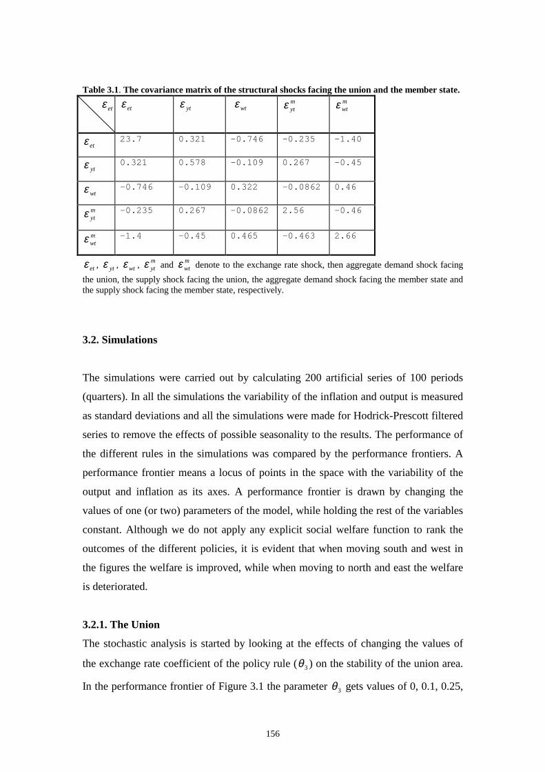
156

Table 3.1. The covar iance matr ix of the structural shocks facing the union and the member state.

etε ytε wtε m

ytε mwtε

etε 23.7 0.321 -0.746 -0.235 -1.40

ytε 0.321 0.578 -0.109 0.267 -0.45

wtε -0.746 -0.109 0.322 -0.0862 0.46

mytε -0.235 0.267 -0.0862 2.56 -0.46

mwtε -1.4 -0.45 0.465 -0.463 2.66

etε , ytε , wtε , mytε and m

wtε denote to the exchange rate shock, then aggregate demand shock facing

the union, the supply shock facing the union, the aggregate demand shock facing the member state and the supply shock facing the member state, respectively.

3.2. Simulations

The simulations were carried out by calculating 200 artificial series of 100 periods

(quarters). In all the simulations the variabilit y of the inflation and output is measured

as standard deviations and all the simulations were made for Hodrick-Prescott filtered

series to remove the effects of possible seasonality to the results. The performance of

the different rules in the simulations was compared by the performance frontiers. A

performance frontier means a locus of points in the space with the variabilit y of the

output and inflation as its axes. A performance frontier is drawn by changing the

values of one (or two) parameters of the model, while holding the rest of the variables

constant. Although we do not apply any explicit social welfare function to rank the

outcomes of the different policies, it is evident that when moving south and west in

the figures the welfare is improved, while when moving to north and east the welfare

is deteriorated.

3.2.1. The Union

The stochastic analysis is started by looking at the effects of changing the values of

the exchange rate coeff icient of the policy rule ( 3θ ) on the stabilit y of the union area.

In the performance frontier of Figure 3.1 the parameter 3θ gets values of 0, 0.1, 0.25,

etε

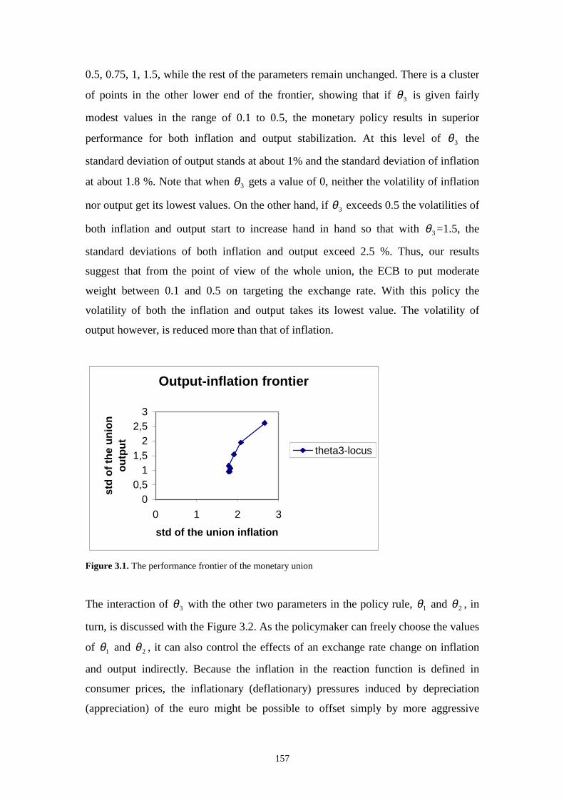
157

0.5, 0.75, 1, 1.5, while the rest of the parameters remain unchanged. There is a cluster

of points in the other lower end of the frontier, showing that if 3θ is given fairly

modest values in the range of 0.1 to 0.5, the monetary policy results in superior

performance for both inflation and output stabili zation. At this level of 3θ the

standard deviation of output stands at about 1% and the standard deviation of inflation

at about 1.8 %. Note that when 3θ gets a value of 0, neither the volatilit y of inflation

nor output get its lowest values. On the other hand, if 3θ exceeds 0.5 the volatiliti es of

both inflation and output start to increase hand in hand so that with 3θ =1.5, the

standard deviations of both inflation and output exceed 2.5 %. Thus, our results

suggest that from the point of view of the whole union, the ECB to put moderate

weight between 0.1 and 0.5 on targeting the exchange rate. With this policy the

volatilit y of both the inflation and output takes its lowest value. The volatilit y of

output however, is reduced more than that of inflation.

Output-inflation frontier

00,5

11,5

22,5

3

0 1 2 3

std of the union inflation

std

of

the

un

ion

o

utp

ut

theta3-locus

Figure 3.1. The performance frontier of the monetary union

The interaction of 3θ with the other two parameters in the policy rule, 1θ and 2θ , in

turn, is discussed with the Figure 3.2. As the policymaker can freely choose the values

of 1θ and 2θ , it can also control the effects of an exchange rate change on inflation

and output indirectly. Because the inflation in the reaction function is defined in

consumer prices, the inflationary (deflationary) pressures induced by depreciation

(appreciation) of the euro might be possible to offset simply by more aggressive

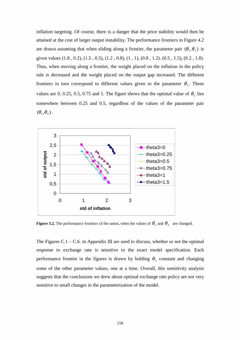
158

inflation targeting. Of course, there is a danger that the price stabilit y would then be

attained at the cost of larger output instabilit y. The performance frontiers in Figure 4.2

are drawn assuming that when sliding along a frontier, the parameter pair ),( 21 θθ is

given values (1.8 , 0.2), (1.5 , 0.5), (1.2 , 0.8), (1 , 1), (0.8 , 1.2). (0.5 , 1.5), (0.2 , 1.8).

Thus, when moving along a frontier, the weight placed on the inflation in the policy

rule is decreased and the weight placed on the output gap increased. The different

frontiers in turn correspond to different values given to the parameter 3θ . These

values are 0, 0.25, 0.5, 0.75 and 1. The figure shows that the optimal value of 3θ lies

somewhere between 0.25 and 0.5, regardless of the values of the parameter pair

),( 21 θθ .

0

0,5

1

1,5

2

2,5

3

0 1 2 3

std of inflation

std

of

ou

tpu

t

theta3=0theta3=0.25theta3=0.5theta3=0.75theta3=1theta3=1.5

Figure 3.2. The performance frontiers of the union, when the values of 1θ and 2θ are changed.

The Figures C.1 – C.6. in Appendix III are used to discuss, whether or not the optimal

response to exchange rate is sensitive to the exact model specification. Each

performance frontier in the figures is drawn by holding 3θ constant and changing

some of the other parameter values, one at a time. Overall , this sensitivity analysis

suggests that the conclusions we drew about optimal exchange rate policy are not very

sensitive to small changes in the parameterization of the model.

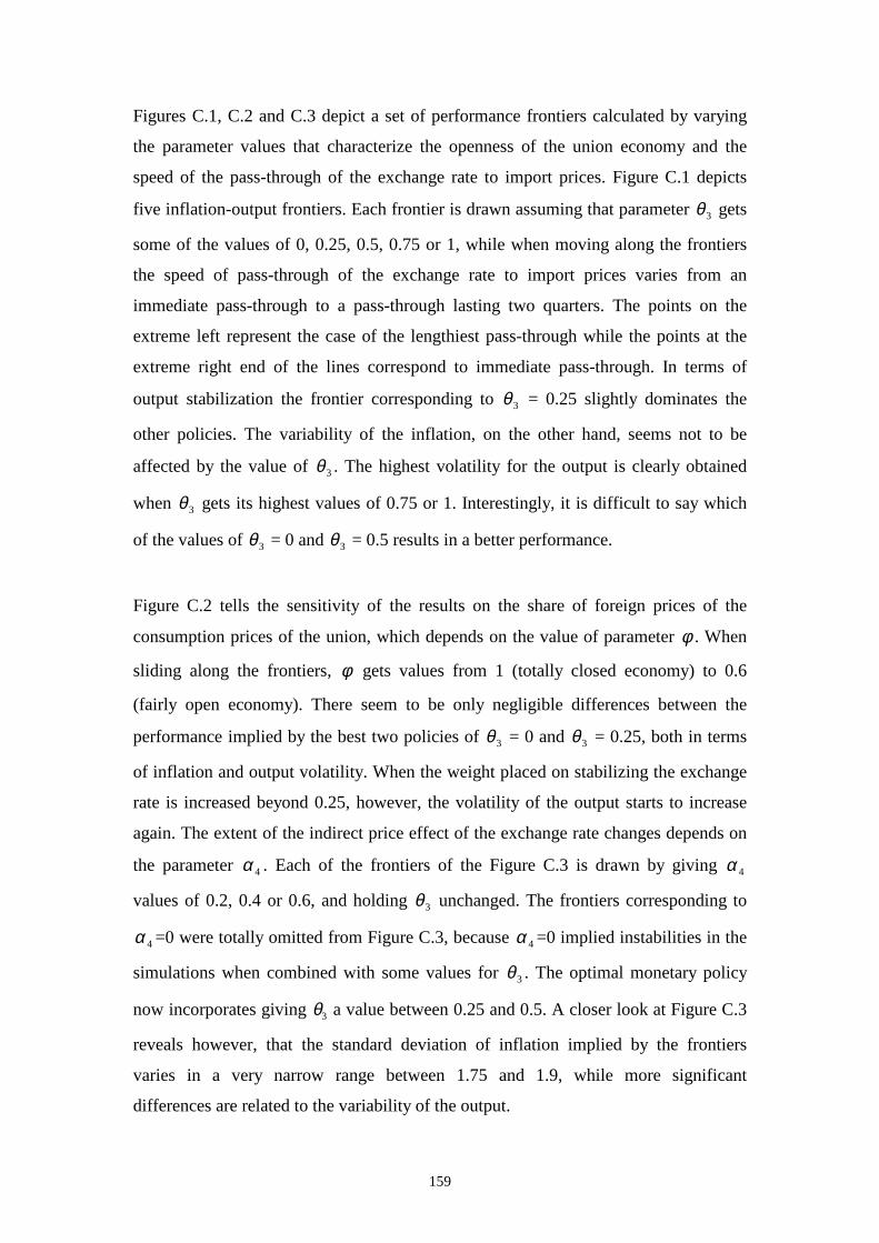
159

Figures C.1, C.2 and C.3 depict a set of performance frontiers calculated by varying

the parameter values that characterize the openness of the union economy and the

speed of the pass-through of the exchange rate to import prices. Figure C.1 depicts

five inflation-output frontiers. Each frontier is drawn assuming that parameter 3θ gets

some of the values of 0, 0.25, 0.5, 0.75 or 1, while when moving along the frontiers

the speed of pass-through of the exchange rate to import prices varies from an

immediate pass-through to a pass-through lasting two quarters. The points on the

extreme left represent the case of the lengthiest pass-through while the points at the

extreme right end of the lines correspond to immediate pass-through. In terms of

output stabili zation the frontier corresponding to 3θ = 0.25 slightly dominates the

other policies. The variabilit y of the inflation, on the other hand, seems not to be

affected by the value of 3θ . The highest volatilit y for the output is clearly obtained

when 3θ gets its highest values of 0.75 or 1. Interestingly, it is diff icult to say which

of the values of 3θ = 0 and 3θ = 0.5 results in a better performance.

Figure C.2 tells the sensitivity of the results on the share of foreign prices of the

consumption prices of the union, which depends on the value of parameter φ . When

sliding along the frontiers, φ gets values from 1 (totally closed economy) to 0.6

(fairly open economy). There seem to be only negligible differences between the

performance implied by the best two policies of 3θ = 0 and 3θ = 0.25, both in terms

of inflation and output volatilit y. When the weight placed on stabili zing the exchange

rate is increased beyond 0.25, however, the volatilit y of the output starts to increase

again. The extent of the indirect price effect of the exchange rate changes depends on

the parameter 4α . Each of the frontiers of the Figure C.3 is drawn by giving 4α

values of 0.2, 0.4 or 0.6, and holding 3θ unchanged. The frontiers corresponding to

4α =0 were totally omitted from Figure C.3, because 4α =0 implied instabiliti es in the

simulations when combined with some values for 3θ . The optimal monetary policy

now incorporates giving 3θ a value between 0.25 and 0.5. A closer look at Figure C.3

reveals however, that the standard deviation of inflation implied by the frontiers

varies in a very narrow range between 1.75 and 1.9, while more significant

differences are related to the variabilit y of the output.

160

The sensitivity of the result can also be discussed in light of the assumptions made

about the rate of forward-lookingness of the union economy. It depends on the values

of parameters 1α and 21

α , which measure the forward-lookingness of the goods

markets and 0χ , which captures the forward-lookingness of the wage-price process.

Figure C.4, which plots the performance frontiers for 1α shows that the output seems

to reach its lowest standard deviation with 3θ in a range of 0 to 0.5. The points of the

frontiers corresponding to these values of 3θ are clustered very close to each other so

that it does not seem to make a difference which the exact value for 3θ is in that

range. When the value of 3θ is increased beyond 0.5, the volatilit y of output starts to

increase. The volatilit y of inflation still seems to be fairly unaffected by the values of

1α and 3θ , remaining at the level of about 2 %, regardless of the values of these

parameters. The shape of the frontiers also reveals that in the more forward looking

goods (that is, with relatively small 1α and large 2α ) market the volatilit y of output is

lower regardless of the value of 3θ .

Figure C.5 shows the performance frontiers when 0χ is given values 0, 0.25 and 0.521

holding 3θ constant. The excessively backward looking wage-price process with

0χ =0 corresponds to the left ends of the frontiers, whereas the baseline case of

0χ =0.5 corresponds to the right ends of the frontiers. The volatilit y of inflation seems

to be sensitive on the forward-lookingness of the job markets so that the fully

backward looking wage-price process results in considerably higher volatilit y of

inflation than the moderately backward looking process (0.7 % vs. 2 %). The result

can be explained by the important role of the contracting process in the determination

of the prices in our model. When it comes to the optimal monetary policy, the

frontiers of 3θ = 0 and 3θ = 0.25 again imply superior performance for output

stabilit y. For the inflation stabilit y the value of 3θ does not seem to make a difference.

21 If 0χ gets a value above 0.5, the model did no more have a sensible solution.

161

Figure 3.3 below finally sums up our discussion about the sensitivity of the results to

the parameter values of the model. Figure is drawn assuming that the union is both

more open with 8.0=φ , 4.04 =α and more forward looking with 2.01 =α . From the

point of view of the union economy, the optimal value for 3θ lies now somewhere

between 0.25 and 1. Thus, for a more open economy than the euro area, our model

would suggest more weight put on stabili sing the exchange rate. The extreme policies

of either 3θ =0 or 3θ =1.5 clearly result in inferior outcomes, however.

0

0,5

1

1,5

2

2,5

3

0 1 2 3

std of inflation

std

of

ou

tpu

t theta3=0theta3=0.25theta3=0.5theta3=0.75theta3=1theta3=1.5

Figure 3.3 The performance frontiers of the union when several parameters affecting its openness are

changed at a time.

3.2.2 The member state

Figure 3.4 below plots the performance frontiers of both the union and the member

state in the same figure. It is seen that the frontier of the member state is located

relatively far to the north-east from the frontier of the whole union. Hence, although

the structural differences between the member state and the rest of the union, after all ,

are rather small i n the baseline parameterisation, the volatilit y of both inflation and

output of the member state seem to be significantly larger than those of the union on

average. The relatively poor performance of the member economy is related

particularly to the volatilit y of its output. It lies between 6 % and 9 %, while the

volatilit y of the member state inflation levels between 2 % and 3 %.

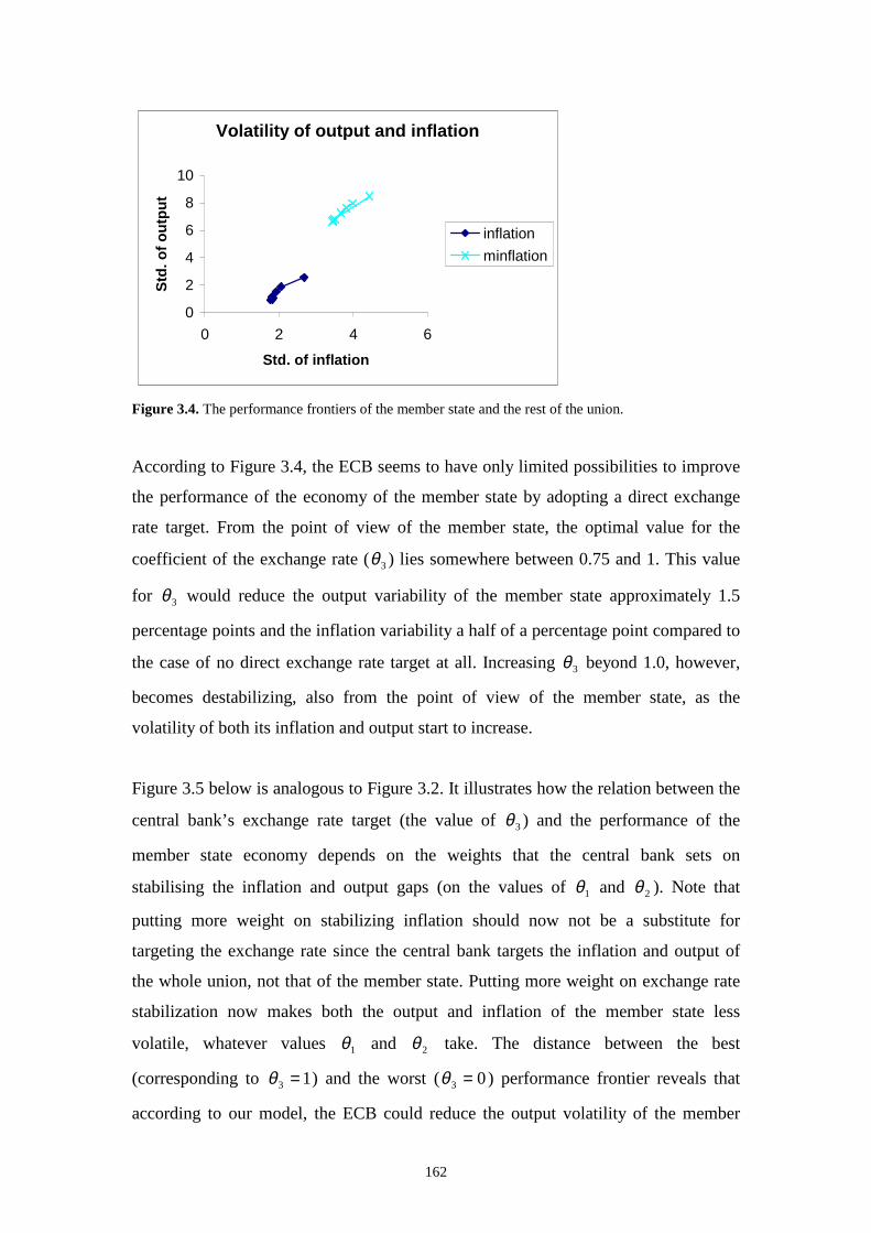
162

Volatility of output and inflation

0

2

4

6

8

10

0 2 4 6

Std. of inflation

Std

. of

ou

tpu

t

inflation

minflation

Figure 3.4. The performance frontiers of the member state and the rest of the union.

According to Figure 3.4, the ECB seems to have only limited possibiliti es to improve

the performance of the economy of the member state by adopting a direct exchange

rate target. From the point of view of the member state, the optimal value for the

coeff icient of the exchange rate ( 3θ ) lies somewhere between 0.75 and 1. This value

for 3θ would reduce the output variabilit y of the member state approximately 1.5

percentage points and the inflation variabilit y a half of a percentage point compared to

the case of no direct exchange rate target at all . Increasing 3θ beyond 1.0, however,

becomes destabili zing, also from the point of view of the member state, as the

volatilit y of both its inflation and output start to increase.

Figure 3.5 below is analogous to Figure 3.2. It ill ustrates how the relation between the

central bank’s exchange rate target (the value of 3θ ) and the performance of the

member state economy depends on the weights that the central bank sets on

stabili sing the inflation and output gaps (on the values of 1θ and 2θ ). Note that

putting more weight on stabili zing inflation should now not be a substitute for

targeting the exchange rate since the central bank targets the inflation and output of

the whole union, not that of the member state. Putting more weight on exchange rate

stabili zation now makes both the output and inflation of the member state less

volatile, whatever values 1θ and 2θ take. The distance between the best

(corresponding to 13 =θ ) and the worst ( 03 =θ ) performance frontier reveals that

according to our model, the ECB could reduce the output volatilit y of the member

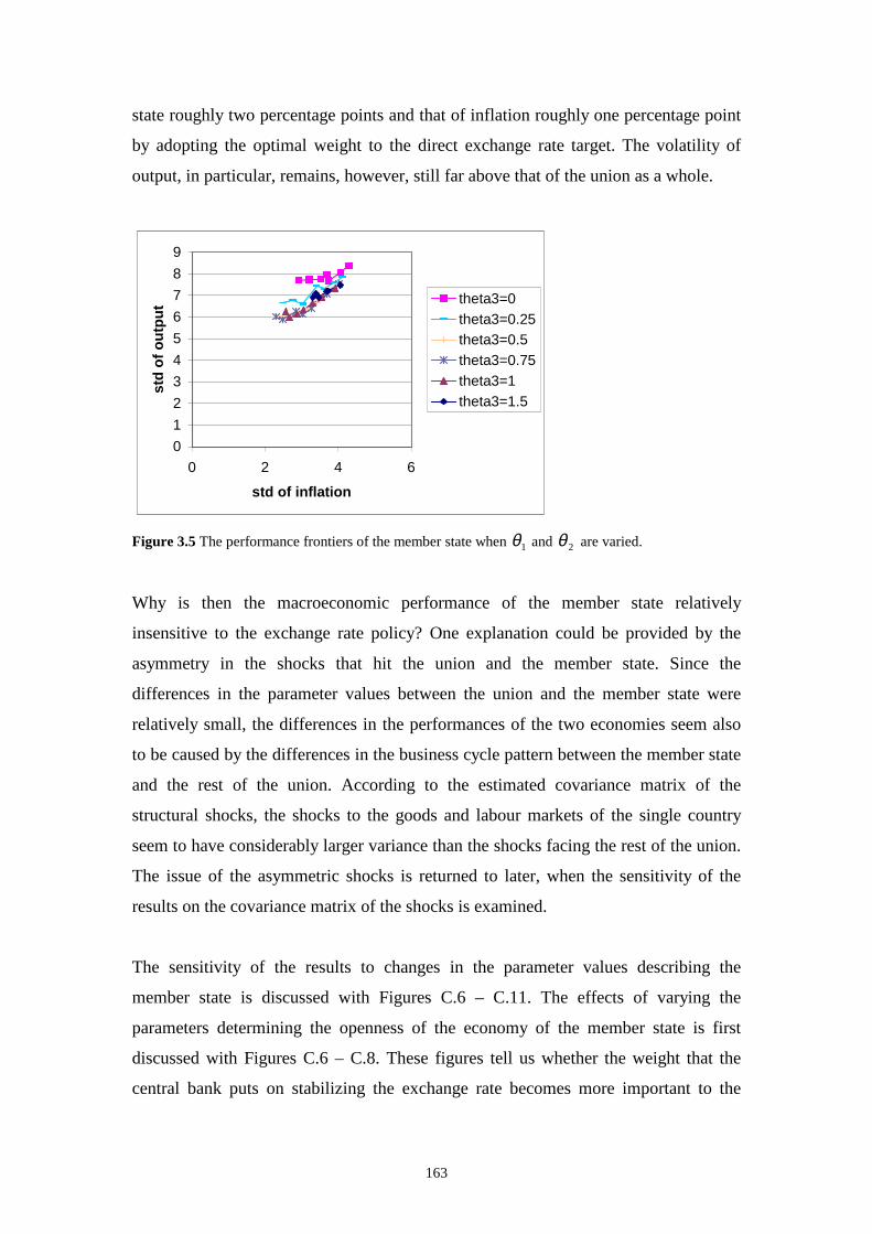
163

state roughly two percentage points and that of inflation roughly one percentage point

by adopting the optimal weight to the direct exchange rate target. The volatili ty of

output, in particular, remains, however, still far above that of the union as a whole.

0

1

2

3

4

5

6

7

8

9

0 2 4 6

std of inflation

std

of

ou

tpu

t theta3=0theta3=0.25theta3=0.5theta3=0.75theta3=1theta3=1.5

Figure 3.5 The performance frontiers of the member state when 1θ and 2θ are varied.

Why is then the macroeconomic performance of the member state relatively

insensitive to the exchange rate policy? One explanation could be provided by the

asymmetry in the shocks that hit the union and the member state. Since the

differences in the parameter values between the union and the member state were

relatively small , the differences in the performances of the two economies seem also

to be caused by the differences in the business cycle pattern between the member state

and the rest of the union. According to the estimated covariance matrix of the

structural shocks, the shocks to the goods and labour markets of the single country

seem to have considerably larger variance than the shocks facing the rest of the union.

The issue of the asymmetric shocks is returned to later, when the sensitivity of the

results on the covariance matrix of the shocks is examined.

The sensitivity of the results to changes in the parameter values describing the

member state is discussed with Figures C.6 – C.11. The effects of varying the

parameters determining the openness of the economy of the member state is first

discussed with Figures C.6 – C.8. These figures tell us whether the weight that the

central bank puts on stabili zing the exchange rate becomes more important to the

164

member state as it becomes more open against the world outside the union. The

openness is measured as the share of goods (κ ) in its consumption bundle that the

member state imports from outside the union, the sensitivity of the export demand of

the member state on the exchange rate of the euro ( 4β ), and the speed of the pass-

through of the exchange rate to consumption prices in the member state. Figure C.9,

in turn, ill ustrates the sensitivity of the results to the degree of integration of the goods

market between the member state and the rest of the union. The degree of integration

is measured by value of 5β that determines how sensitive the aggregate demand of

the member economy is to the output of the union.

Overall , our qualitative conclusions about the ECB’s optimal exchange rate policy,

from the point of view of the member state, do not seem to be sensitive regarding

small changes in the parameter values that describe the openness of the member

economy in our model. The volatilit y of both the inflation and output are at their

lowest level when 3θ gets a value of 0.75 or 0.5, whereas putting zero weight on the

exchange rate, for example, clearly implies less favourable outcome. Quantitatively,

too, the results remain roughly unchanged for all the alternative parameter values

considered. If the central bank would pursue optimal exchange rate policy from the

point of view of the member state, that would lead to a two percentage point decrease

in the standard deviation of output and roughly one percentage point in that of

inflation.

Parameter 5β determines how deeply the goods markets of the member state are

integrated with the goods markets of the rest of the union. The sensitivity of the

performance of the member state economy to changes in 5β is shown in Figure C.9. It

is seen that neither the volatilit y of inflation nor the output of the member state can be

significantly reduced by integrating the goods markets closer together. All the points

of the frontiers are concentrated close together. This finding is against the basic result

of the literature on optimal currency areas, according to which integrating the goods

markets of the countries of a currency area closer together effectively protects them

from the problems of asymmetric economic shocks. Our previous conclusions

concerning the optimal monetary policy however still remain valid. By adopting a

165

relatively active exchange rate policy with 3θ set as 0.5 or 0.75 the ECB can reduce

the standard deviation of member state inflation from around 4% to about 3% and the

standard deviation of output from the level of 8% to the level of 6 %.

Figures C.10 and C.11 show the robustness of the results to the assumptions about the

degree of forward-lookingness of the goods and labour markets of the member state.

Figure C.10 at first shows that irrespective of the rate of forward lookingness of the

goods market (values for 1β and 2β ), active exchange rate policy reduces the

volatilit y of inflation and output. Moreover, it can be seen that the points in the

frontiers that correspond to markedly forward looking goods market in the member

state (relatively low values of 1β and high values for 2β ) are much closer to each

other than the points that correspond to markedly backward-looking goods market.

Thus, if the goods markets of the member state are significantly backward looking,

the exchange rate policy seems to matter more to the performance of its economy.

Although the optimal value of 3θ does not seem to depend on the rate of forward-

lookingness of the goods market of the member state, the rate of forward lookingness

in itself seems to affect to the volatilit y of the inflation and output of the member

state. In simulations with 8.01 =α and 5.00 =ψ the standard deviation of inflation

took values around 3 % - 4 % and that of output between 6 % and 8%, irrespective of

the parameter values describing either the monetary policy or the openness of the

economy. When either the goods markets or the labour markets were assumed to be

more forward-looking, the volatilit y of both inflation and output, however, decreased

sharply. When either 01 =α or 10 =ψ , the standard deviation of inflation was

reduced near 2 % and the standard deviation of output near the level of 4 %.

Figure C.11 then confirms the robustness of our previous results to the assumptions

made on the forward-lookingness of the labour markets. The worst outcomes again

seem to result from the policy with no exchange rate target at all , while the best

performance seems to be achieved with 3θ set either to 0.5 or 0.75. In the simulations

the value of 0ψ ranged only between 0.5 and 1, because at values below 0.5 the

system exploded.

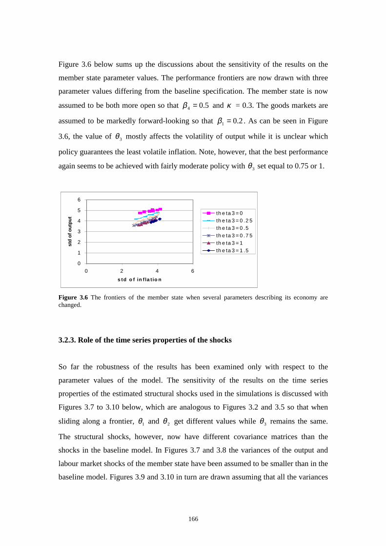
166

Figure 3.6 below sums up the discussions about the sensitivity of the results on the

member state parameter values. The performance frontiers are now drawn with three

parameter values differing from the baseline specification. The member state is now

assumed to be both more open so that 5.04 =β and κ = 0.3. The goods markets are

assumed to be markedly forward-looking so that 2.01 =β . As can be seen in Figure

3.6, the value of 3θ mostly affects the volatilit y of output while it is unclear which

policy guarantees the least volatile inflation. Note, however, that the best performance

again seems to be achieved with fairly moderate policy with 3θ set equal to 0.75 or 1.

0

1

2

3

4

5

6

0 2 4 6

s td o f in f la t io n

std

of

ou

tpu

t

th e ta 3 = 0th e ta 3 = 0 .2 5th e ta 3 = 0 .5th e ta 3 = 0 .7 5th e ta 3 = 1th e ta 3 = 1 .5

Figure 3.6 The frontiers of the member state when several parameters describing its economy are changed.

3.2.3. Role of the time series properties of the shocks

So far the robustness of the results has been examined only with respect to the

parameter values of the model. The sensitivity of the results on the time series

properties of the estimated structural shocks used in the simulations is discussed with

Figures 3.7 to 3.10 below, which are analogous to Figures 3.2 and 3.5 so that when

sliding along a frontier, 1θ and 2θ get different values while 3θ remains the same.

The structural shocks, however, now have different covariance matrices than the

shocks in the baseline model. In Figures 3.7 and 3.8 the variances of the output and

labour market shocks of the member state have been assumed to be smaller than in the

baseline model. Figures 3.9 and 3.10 in turn are drawn assuming that all the variances

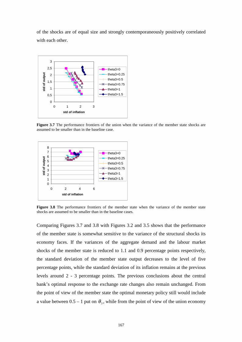
167

of the shocks are of equal size and strongly contemporaneously positively correlated

with each other.

0

0,5

1

1,5

2

2,5

3

0 1 2 3

std of inflation

std

of

ou

tpu

t

theta3=0

theta3=0.25

theta3=0.5

theta3=0.75

theta3=1

theta3=1.5

Figure 3.7 The performance frontiers of the union when the variance of the member state shocks are assumed to be smaller than in the baseline case.

012345678

0 2 4 6

std of inflation

std

of

ou

tpu

t

theta3=0

theta3=0.25

theta3=0.5

theta3=0.75

theta3=1

theta3=1.5

Figure 3.8 The performance frontiers of the member state when the variance of the member state shocks are assumed to be smaller than in the baseline cases.

Comparing Figures 3.7 and 3.8 with Figures 3.2 and 3.5 shows that the performance

of the member state is somewhat sensitive to the variance of the structural shocks its

economy faces. If the variances of the aggregate demand and the labour market

shocks of the member state is reduced to 1.1 and 0.9 percentage points respectively,

the standard deviation of the member state output decreases to the level of f ive

percentage points, while the standard deviation of its inflation remains at the previous

levels around 2 - 3 percentage points. The previous conclusions about the central

bank’s optimal response to the exchange rate changes also remain unchanged. From

the point of view of the member state the optimal monetary policy still would include

a value between 0.5 – 1 put on 3θ , while from the point of view of the union economy

168

the value of 3θ should lie somewhere at the level of 0 – 0.5. It is expected that the

results for the union remain unchanged, since the central bank does not react to

shocks in the markets of the small member state.

According to Figures 3.9 and 3.10, on the other hand, when the shocks become highly

correlated with each other, the value of 3θ loses its significance. It is seen in Figure

3.10 that all the six performance frontiers of the member economy are of almost equal

shape. The performance frontiers of the union in Figure 3.10 also look much alike.

From Figure 3.10 it can also be seen that when the shocks are highly correlated, it is

possible to still reduce the volatilit y of output of the member state. The left ends of

the performance frontiers (corresponding to values around 1.5 for the inflation

coeff icient 1θ and very low values of the output gap coefficient 2θ ) imply that the

standard deviation for member state output can be reduced to somewhere near the

level of 3 %. On the other hand, if the parameters of the reaction function are not near

their optimal levels, the model implies rather high volatiliti es for the output and

inflation of the member state.

00,5

11,5

22,5

33,5

0 2 4 6

std of inflation

std

of

ou

tpu

t

theta3=0

theta3=0.25

theta3=0.5

theta3=0.75

theta3=1

theta3=1.5

Figure 3.9 The performance frontiers of the union when the structural shocks between the member state and the union are strongly correlated.

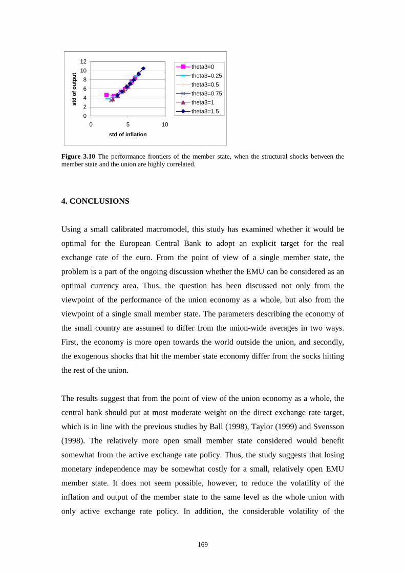
169

0

2

4

6

8

10

12

0 5 10

std of inflation

std

of o

utp

ut

theta3=0

theta3=0.25

theta3=0.5

theta3=0.75

theta3=1

theta3=1.5

Figure 3.10 The performance frontiers of the member state, when the structural shocks between the member state and the union are highly correlated.

4. CONCLUSIONS

Using a small calibrated macromodel, this study has examined whether it would be

optimal for the European Central Bank to adopt an explicit target for the real

exchange rate of the euro. From the point of view of a single member state, the

problem is a part of the ongoing discussion whether the EMU can be considered as an

optimal currency area. Thus, the question has been discussed not only from the

viewpoint of the performance of the union economy as a whole, but also from the

viewpoint of a single small member state. The parameters describing the economy of

the small country are assumed to differ from the union-wide averages in two ways.

First, the economy is more open towards the world outside the union, and secondly,

the exogenous shocks that hit the member state economy differ from the socks hitting

the rest of the union.

The results suggest that from the point of view of the union economy as a whole, the

central bank should put at most moderate weight on the direct exchange rate target,

which is in line with the previous studies by Ball (1998), Taylor (1999) and Svensson

(1998). The relatively more open small member state considered would benefit

somewhat from the active exchange rate policy. Thus, the study suggests that losing

monetary independence may be somewhat costly for a small , relatively open EMU

member state. It does not seem possible, however, to reduce the volatilit y of the

inflation and output of the member state to the same level as the whole union with

only active exchange rate policy. In addition, the considerable volatilit y of the

170

member state output seemed to result more from the size and the symmetry of the

structural shocks that hit its economy than from its greater d ree of openness.

REFERENCES Ball , L. (1998) Policy Rules for Open Economies NBER Working Paper 6760 Batini, N. – Haldane, A. G. (1998) Forward-looking rules for monetary policy Bank of England Working Paper Series No 91. Bayoumi, T. – Eichengreen, B. (1992) Shocking Aspects of European Monetary Unification NBER Working Paper No. 3949 Benhabib, J. – Smitt-Grohe S. – Uribe M. (2001) The Perils of Taylor Rules Journal of Economic Theory, Vol. 96, p.40-69. Clarida, R. – Gali , J. – Gertler, M. (1999) The Science of Monetary Policy: A New Keynesian Perspective Journal of Economic Literature, Vol. XXXV II, PP. 1661 – 1707. Coenen, G. – Wieland, V. (2000) A Small Estimated Euro Area Model with Rational Expectations and Nominal Rigidities ECB Working Paper n.o. 30. Dornbusch, R. – Favero, C. A. – Giavazzi, F. (1998) The Immediate Challenges for the European Central Bank NBER Working Paper 6369. Goldberg, K. P. – Knetter, M. M. (1997) Goods Pr ices and Exchange Rates: What have we learned? Journal of Economic Literature, Sep 1997, Vol. XXXV , Number 3, p. 1243 – 1272. Kozicki, S. (1998) How Useful are Taylor Rules for M onetary Policy? Federal Reserve Bank of Kansas City Economic Review II /1999.

171

Mayes, D. G. – , Virén, M. (1998) The Exchange Rate and Monetary Conditions in the Euro Area. Bank of Finland Discussion Papers 27/1998. McCallum, B. J. (1999) Recent Developments in the Analysis of Monetary Policy Rules Homer Jones Memorial Lecture March 11, 1999. Carnegie Mellon University. McCallum, B. T. – Nelson, E. (1997) An Optimizing IS-LM Specification for M onetary Policy and Business Cycle Analysis. NBER Working Paper 5875 Peersman, G. – Smets, F. (1998) Uncertainty and the Taylor r ule in a simple model of the euro-area economy Federal Reserve Bank of San Fransisco, Proceedings 266. Ranki, S. (2000) Does the Euro Exchange Rate Matter? ETLA Discussion Papers no. 729 Rogoff , K. (2001) Why Not a Global Currency? American Economic Review, Vol. 91, No 2. Schelkle, W. (2001) The Optimum Currency Area Approach to European Monetary Integration: Framework of Debate or Dead End? South Bank European Papers 2/2001. South Bank University. London. Svensson, L. E. O. (1998) Open-Economy Inflation Targeting NBER Working Paper 6545 Taylor, J. B. (1999) The Robustness and Eff iciency of Monetary Policy Rules as Guidelines for Interest Rate Sett ing by the European Central Bank Journal of Monetary Economics, June 1999, 43(3), p. 655-79. Taylor, J. B. (2001) The Role of the Exchange Rate in Monetary-Policy Rules American Economic Review, Vol. 91, No 2. Uhlig, H. (1999) A toolkit for analysing nonlinear dynamic stochastic models easily In “Computational Methods for the Study of Dynamic Economies” , edited by Marimon, R. and Scott, A. Oxford University Press 1999.

172

Woodford, M. (1999) Inflation Stabili zation and Welfare. Workin Paper, Princeton University, June. (Available at http://www.princeton.edu/~woodford/) Woodford, M. (2000) A Neo-Wickselli an Framework for the Analysis of Monetary Policy Manuscript. Princeton University. (Available at http://www.princeton.edu/~woodford/) Woodford, M. (2001) The Taylor Rule and Optimal Monetary Policy American Economic Review Vol. 91 No. 2. P. 232 – 237.

173

APPENDIX I The calculation of the unconditional var iances of inflation and output The conditional moments were calculated from simulated series. The simulation horizon of each series was 100 periods and the simulation was repeated x times, so that totally 100x sets of solution values was available for the calculation of the unconditional moments.

Denote the estimated covariance matrix of the structural shocks by mm× matrix Σ ,

computed as 'ZZ ˆˆ)/1( T , where Z is the Tm× matrix of the estimated values of the exogenous structural shocks. If the z shocks are IID distributed, the set of shocks used in the stochastic simulation can be obtained from a simple transformation of Σ . To generate the shocks, the matrix Σ is decomposed into two triangular matrices that, when calculated together, yield the original matrix Σ . If the rank condition holds (T > m), there exists a unique such decomposition, PP'=� such that P is lower triangular and 'P is upper triangular. The initial (t=0) values for the exogenous shocks z were calculated by first drawing m values from a standard normal distribution. Let’s denote the vector of these values by

1e . These white noise disturbances were then turned into structural shocks by

1*1 Pez = . Using the values *

1z and the equations of the recursive law of motion, it is

then possible to calculate values of 1x and 1y . Another draw from a normal

distribution is then made for calculating values for *2z , 2x and 2y . The process is

then repeated until N values are obtained. Assuming that the historical residuals are independently and identically distributed implies that in the equation all elements in the matrix N equal to zero. In case that the historical residuals are autocorrelated, the residuals have to be “whiten” before calculating the covariance matrix . Suppose, for example, the first order

autocorrelation t1tt vNzz += − , )N(0,�v vt ≈ . 'ˆ ** PP� v = Now the value for *1z is

obtained from 1*1 ePz *= , where *P is obtained from the Choleski factorization

'ˆ ** PP� v = . The value for *2z is then calculated from 2

**1

*2 ePNzz += .

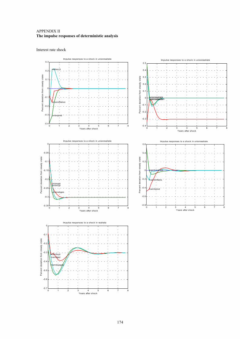
APPENDIX II The impulse responses of deterministic analysis Interest rate shock

0 1 2 3 4 5 6 7 8-0.4

-0.3

-0.2

-0.1

0

0.1

0.2

0.3Impulse responses to a shock in unionrealrate

Years after shock

Per

cent

dev

iatio

n fro

m s

tead

y st

ate

unionprod

unioninflation

realexch

0 1 2 3 4 5 6 7 8-0.4

-0.3

-0.2

-0.1

0

0.1

0.2

0.3

0.4

0.5Impulse responses to a shock in unionrealrate

Years after shock

Per

cent

dev

iatio

n fro

m s

tead

y st

ate

unionrealrate nominalexch nomininterestr

0 1 2 3 4 5 6 7 8-0.35

-0.3

-0.25

-0.2

-0.15

-0.1

-0.05

0Impulse responses to a shock in unionrealrate

Years after shock

Per

cent

dev

iatio

n fro

m s

tead

y st

ate

unionwages

unioncpi unionppi

0 1 2 3 4 5 6 7 8-0.8

-0.6

-0.4

-0.2

0

0.2

0.4

0.6Impulse responses to a shock in unionrealrate

Years after shock

Per

cent

dev

iatio

n fro

m s

tead

y st

ate

membrealrate

membprod

membinflatio

0 1 2 3 4 5 6 7 8-0.7

-0.6

-0.5

-0.4

-0.3

-0.2

-0.1

0Impulse responses to a shock in realrate

Years after shock

Per

cent

dev

iatio

n fro

m s

tead

y st

ate

membwages

membcpi membppi

174

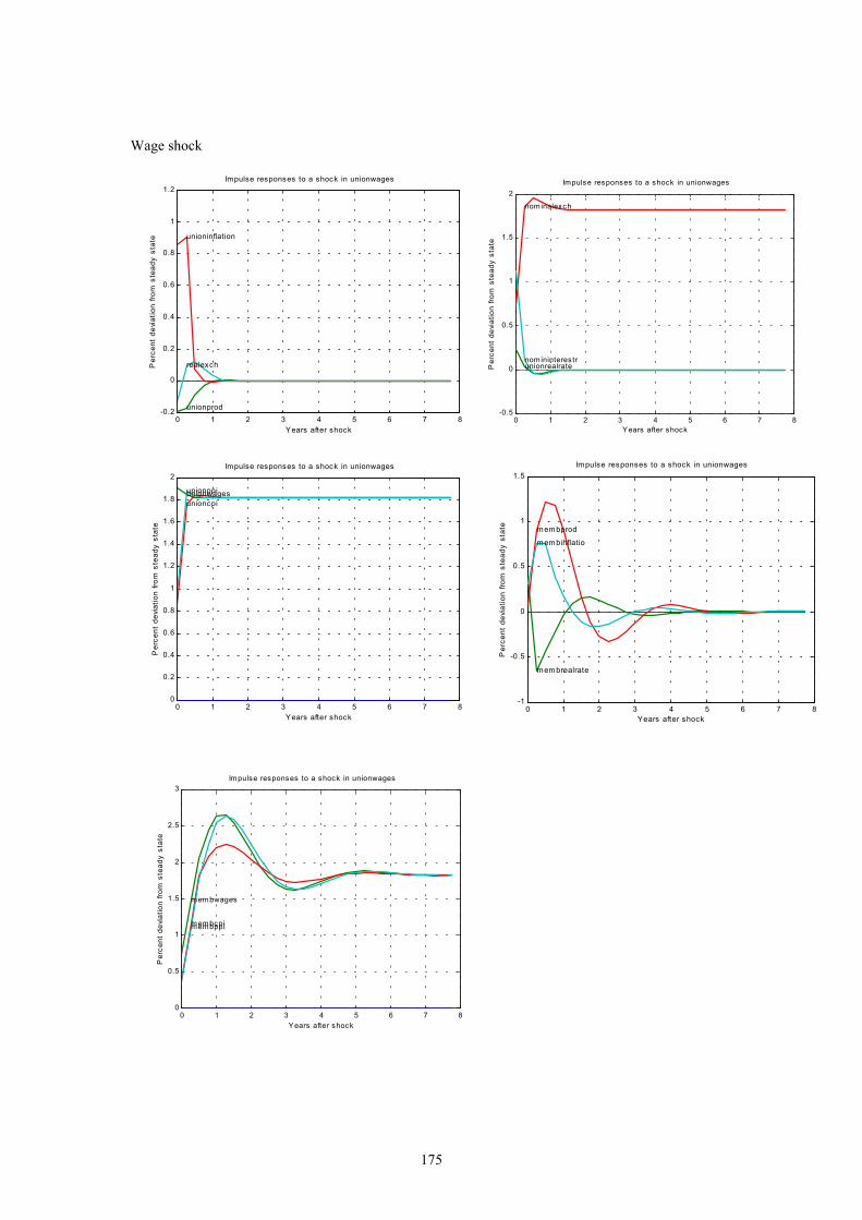
Wage shock

0 1 2 3 4 5 6 7 8-0.2

0

0.2

0.4

0.6

0.8

1

1.2Impulse responses to a shock in unionwages

Years after shock

Per

cent

dev

iatio

n fro

m s

tead

y st

ate

unionprod

unioninflation

realexch

0 1 2 3 4 5 6 7 8-0.5

0

0.5

1

1.5

2Impulse responses to a shock in unionwages

Years after shock

Per

cent

dev

iatio

n fro

m s

tead

y st

ate

unionrealrate

nominalexch

nomininterestr

0 1 2 3 4 5 6 7 80

0.2

0.4

0.6

0.8

1

1.2

1.4

1.6

1.8

2Impulse responses to a shock in unionwages

Years after shock

Per

cent

dev

iatio

n fro

m s

tead

y st

ate

unionwages unioncpi

unionppi

0 1 2 3 4 5 6 7 8-1

-0.5

0

0.5

1

1.5Impulse responses to a shock in unionwages

Years after shock

Per

cent

dev

iatio

n fro

m s

tead

y st

ate

membrealrate

membprod

membinflatio

0 1 2 3 4 5 6 7 80

0.5

1

1.5

2

2.5

3Impulse responses to a shock in unionwages

Years after shock

Per

cent

dev

iatio

n fro

m s

tead

y st

ate

membwages

membcpi membppi

175

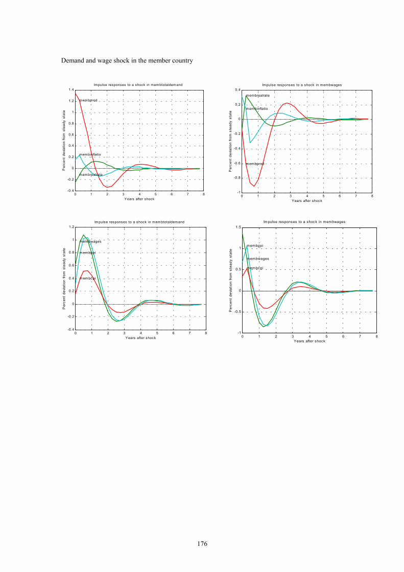
Demand and wage shock in the member country

0 1 2 3 4 5 6 7 8-0.4

-0.2

0

0.2

0.4

0.6

0.8

1

1.2

1.4Impulse responses to a shock in membtotaldemand

Years after shock

Per

cent

dev

iatio

n fro

m s

tead

y st

ate

membrealrate

membprod

membinflatio

0 1 2 3 4 5 6 7 8-1

-0.8

-0.6

-0.4

-0.2

0

0.2

0.4Impulse responses to a shock in membwages

Years after shock

Per

cent

dev

iatio

n fro

m s

tead

y st

ate

membrealrate

membprod

membinflatio

0 1 2 3 4 5 6 7 8-0.4

-0.2

0

0.2

0.4

0.6

0.8

1

1.2Impulse responses to a shock in membtotaldemand

Years after shock

Per

cent

dev

iatio

n fro

m s

tead

y st

ate

membwages

membcpi

membppi

0 1 2 3 4 5 6 7 8-1

-0.5

0

0.5

1

1.5Impulse responses to a shock in membwages

Years after shock

Per

cent

dev

iatio

n fro

m s

tead

y st

ate

membwages

membcpi

membppi

176

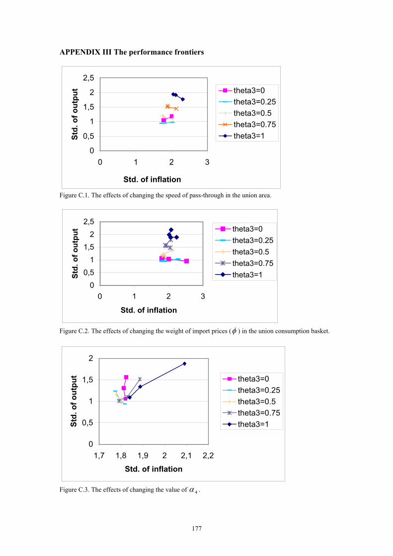
APPENDIX III The performance frontiers

0

0,5

1

1,5

2

2,5

0 1 2 3

Std. of inflation

Std.

of o

utpu

t theta3=0theta3=0.25theta3=0.5theta3=0.75theta3=1

Figure C.1. The effects of changing the speed of pass-through in the union area.

00,51

1,52

2,5

0 1 2 3

Std. of inflation

Std.

of o

utpu

t theta3=0theta3=0.25theta3=0.5theta3=0.75theta3=1

Figure C.2. The effects of changing the weight of import prices ( ) in the union consumption basket. φ

0

0,5

1

1,5

2

1,7 1,8 1,9 2 2,1 2,2Std. of inflation

Std.

of o

utpu

t theta3=0theta3=0.25theta3=0.5theta3=0.75theta3=1

Figure C.3. The effects of changing the value of . 4α

177

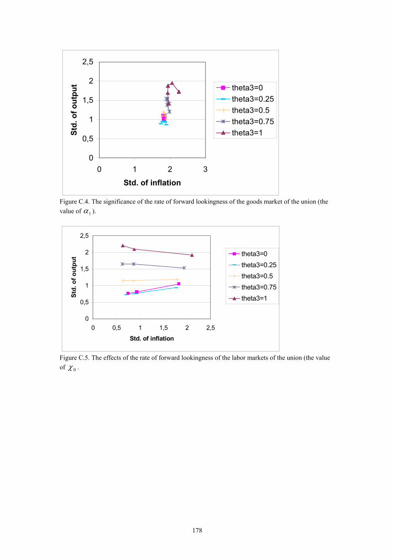
0

0,5

1

1,5

2

2,5

0 1 2 3

Std. of inflation

Std.

of o

utpu

t theta3=0theta3=0.25theta3=0.5theta3=0.75theta3=1

Figure C.4. The significance of the rate of forward lookingness of the goods market of the union (the value of ). 1α

0

0,5

1

1,5

2

2,5

0 0,5 1 1,5 2 2,5

Std. of inflation

Std.

of o

utpu

t theta3=0theta3=0.25theta3=0.5theta3=0.75theta3=1

Figure C.5. The effects of the rate of forward lookingness of the labor markets of the union (the value of . 0χ

178

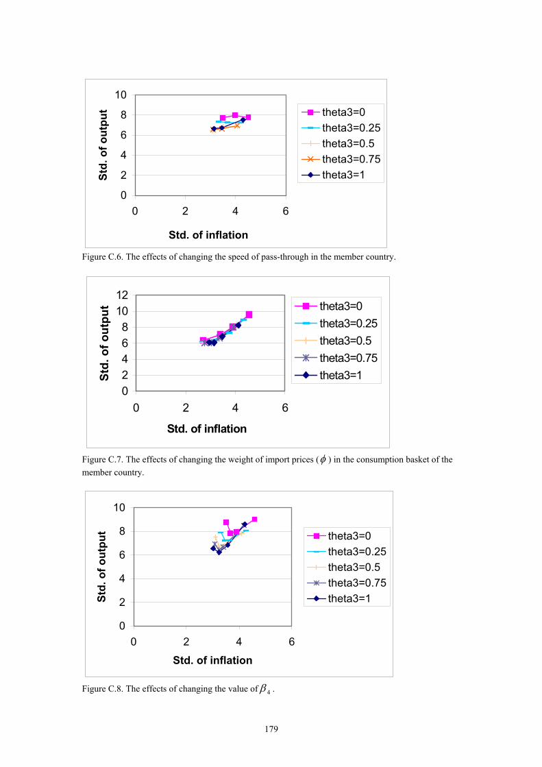
0

2

4

6

8

10

0 2 4 6

Std. of inflation

Std.

of o

utpu

t theta3=0theta3=0.25theta3=0.5theta3=0.75theta3=1

Figure C.6. The effects of changing the speed of pass-through in the member country.

024681012

0 2 4 6

Std. of inflation

Std.

of o

utpu

t theta3=0theta3=0.25theta3=0.5theta3=0.75theta3=1

Figure C.7. The effects of changing the weight of import prices ( ) in the consumption basket of the member country.

φ

0

2

4

6

8

10

0 2 4 6Std. of inflation

Std.

of o

utpu

t theta3=0theta3=0.25theta3=0.5theta3=0.75theta3=1

Figure C.8. The effects of changing the value of . 4β

179

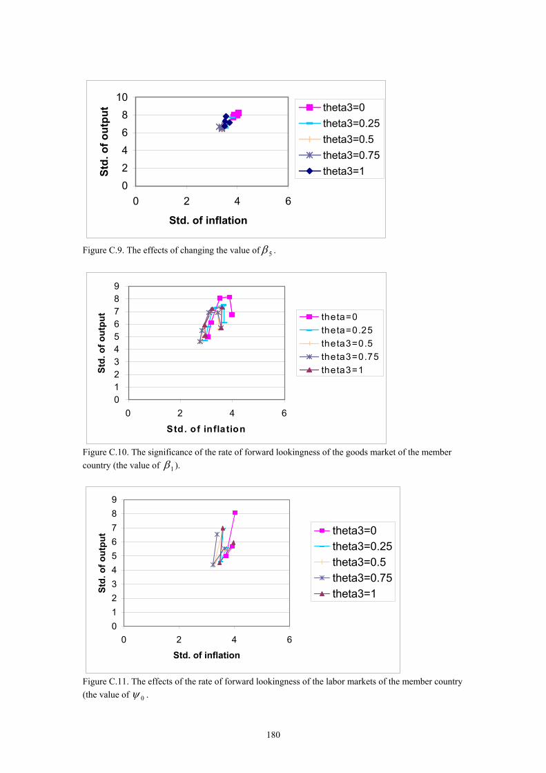
0246810

0 2 4 6

Std. of inflation

Std.

of o

utpu

t theta3=0theta3=0.25theta3=0.5theta3=0.75theta3=1

Figure C.9. The effects of changing the value of . 5β

0123456789

0 2 4 6

Std. of inflation

Std.

of o

utpu

t theta=0theta=0.25theta3=0.5theta3=0.75theta3=1

Figure C.10. The significance of the rate of forward lookingness of the goods market of the member country (the value of ). 1β

0123456789

0 2 4 6Std. of inflation

Std.

of o

utpu

t theta3=0theta3=0.25theta3=0.5theta3=0.75theta3=1

Figure C.11. The effects of the rate of forward lookingness of the labor markets of the member country (the value of 0ψ .

180

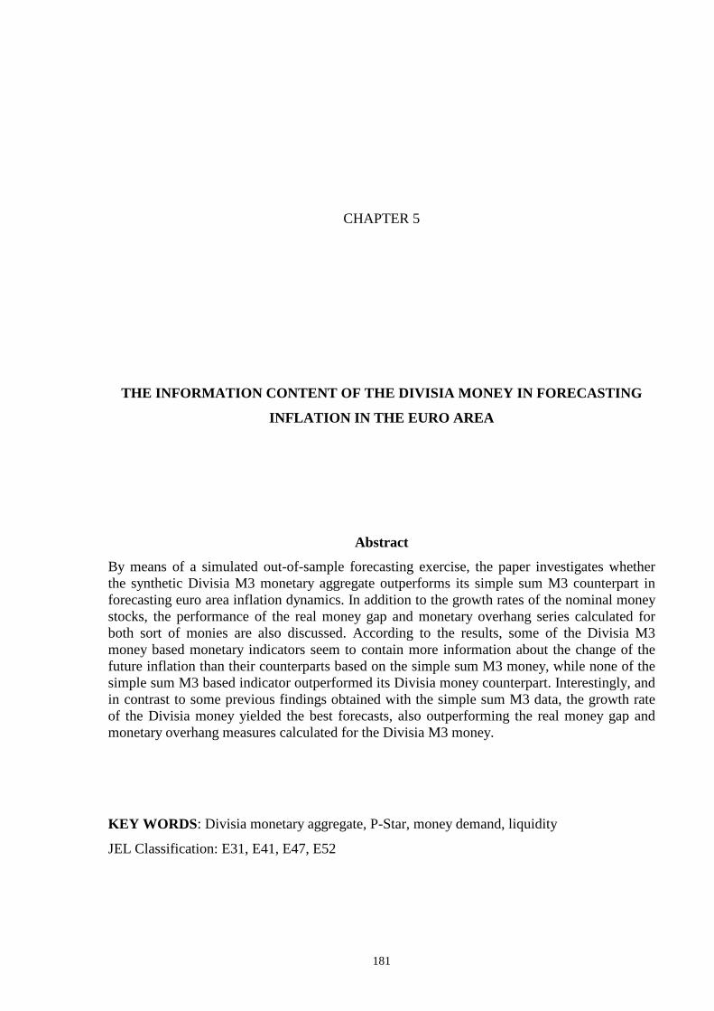
181

CHAPTER 5

THE INFORMATION CONTENT OF THE DIVISIA MONEY IN FORECASTING

INFLATION IN THE EURO AREA

Abstract

By means of a simulated out-of-sample forecasting exercise, the paper investigates whether the synthetic Divisia M3 monetary aggregate outperforms its simple sum M3 counterpart in forecasting euro area inflation dynamics. In addition to the growth rates of the nominal money stocks, the performance of the real money gap and monetary overhang series calculated for both sort of monies are also discussed. According to the results, some of the Divisia M3 money based monetary indicators seem to contain more information about the change of the future inflation than their counterparts based on the simple sum M3 money, while none of the simple sum M3 based indicator outperformed its Divisia money counterpart. Interestingly, and in contrast to some previous findings obtained with the simple sum M3 data, the growth rate of the Divisia money yielded the best forecasts, also outperforming the real money gap and monetary overhang measures calculated for the Divisia M3 money.

KEY WORDS: Divisia monetary aggregate, P-Star, money demand, liquidity

JEL Classification: E31, E41, E47, E52

182

Contents

1. INTRODUCTION 183 2. DIVISIA MONEY 186 2.1. Theoretical background of the Divisia money 186

2.2. Building the synthetic aggregates 187

3. METHODOLOGY 189 3.1. Monetary indicators 189 3.2. Econometric methodology 192 3.3. Data 194

3.4. Money demand equations 196 3.4.1. Estimation of the long-run money demand equations

for the euro area 196 3.4.2. Time series properties of the monetary indicator

variables 199 4. RESULT S 201 5. CONCLUSIONS 205 REFERENCES 207 APPENDIX A 212 APPENDIX B: The line graphs of the relative MSE:s 220

183

1. INTRODUCTION

In the long run, inflation is always and everywhere a monetary phenomenon. This traditional

view is clearly reflected in the ECB’s two-pill ar strategy. While the first of the ECB’s pill ars

refers to a broadly based assessment of the risks to price stabilit y in the Euro area, the second

pill ar establishes a prominent role for the growth rate of nominal M3 money as an information

variable about future inflation. There are, however, some theoretical problems related to the

ECB’s focus on only traditional monetary aggregates such as M1, M2 and M3. The

traditional monetary aggregates are built simply by summing up their component assets,

without explicitl y paying attention to the different degree of liquidity of the components. This

is equivalent to assuming that the component assets are perfect substitutes for each other and

thus, the simple sum aggregates become upward biased estimates of the degree of liquidity of

the economy.

A promising solution to this aggregation problem is provided by the Divisia monetary

aggregates, monetary quantity index numbers based upon both the index number theory and

the economic aggregation theory. The Divisia aggregates are computed as weighted averages

of their components so that the weights are derived from economic theory with optimizing

agents. The weight of a given asset is associated with the opportunity costs of holding that

asset, which measures the liquidity of the asset. Intuitively, the Divisia monetary aggregates

then measure the flow of liquidity services in the economy.

The research problem of this study is then to examine, whether the Divisia M3 monetary

aggregate calculated for the euro-area contains more information on the future euro-area

inflation than the traditional M3 money. If this really is the case, the Divisia monetary

aggregates might provide a useful indicator variable for the ECB to be used instead / along

with the traditional aggregates for forecasting inflation. Instead of only comparing the relative

forecasting performance of the nominal growth rates of the two monies, also the forecasting

performance of a set of monetary indicators measuring the excess liquidity in the economy

(the real money gap and the monetary overhang) are examined. As an econometric method I

use simulated out-of-sample forecasting that has recently been used to similar purposes by

Stock and Watson (1999) and Altimari (2001).

184

Looking at the previous literature on the relation between money and inflation in the economy,

according to the quantity theory of money, there should exist a one-to-one relationship

between money and inflation in the long run. When looking at the previous empirical studies

on the subject, mainly focused on the information content of the traditional monetary

aggregates, the relation between money and inflation in horizons relevant for monetary policy-

making is debatable, however. De Grauwe and Polan (2001), for example, examine

empirically the validity of the basic propositions of the quantity theory of money and conclude

that even the long-run relation between inflation and the growth rate of money breaks down

for low inflation countries.

Moreover, the prominent role of the growth rate of M3 money given in the ECB’s monetary

policy is strongly criti cized in Svensson (2000), mainly because of its lack of predictive power

for inflation1. On the other hand, Altimari (2001), Gerlach and Svensson (2001) and Trecroci

and Vega (2000) study whether the real money gap, the measure for the abundance of real

money in the economy derived from the so-called P-star model, contains additional

information in predicting the Euro area inflation. All these studies confirm that measures

derived from the P-star model really have predictive value for CPI inflation, although

Altimari’s results do not support giving a strong role particularly to the real money gap.

Svensson (2000) also refers to the possible information content of the monetary indicators

derived from the P-star model, emphasizing the important distinction between the level of real

money focused in the P-star model and the growth rate of nominal money that the ECB

actually targets.2 King (2002), Nelson (2002) and Meltzer (2001), in turn discuss the

possibilit y that the real money balances may play a role in the transmission process of

monetary policy that is independent of short term interest rates.

The information content of the Divisia money in predicting inflation in the euro area, in turn,

is discussed in Stracca (2001) and Reimers (2002). Both studies suggest that the Divisia

money actually has additional predictive power for the euro area inflation. Stracca examines

the predictive power of the growth rate of real Divisia money in forecasting future inflation

and output with linear models. Stracca both estimates an equation for the demand of Divisia

1 Moreover, it may make the ECB’s policy less transparent if the significance of the reference value of M3 growth for ECB’s policy is highlighted in rhetoric, while at the same time the ECB in practice ignores even persistent deviations of M3 growth from the reference value (see e.g. Allsopp, 2001). 2 On the other hand, Svensson criticizes the P-star model for a lack of solid microfoundations and its dependence on the unreliable estimates of both real money and output gaps.

185

money in the euro area and builds an unrestricted VAR model with changes in the real Divisia

money as one of the variables. From the impulse responses of the VAR model, Stracca

concludes that the changes in real Divisia money carry some information about the future

inflation and output that is not contained in the stock of M3 money.

Reimers (2002) in turn, examines the properties of several alternative series for the euro area

Divisia money, based on slightly differing methods used to aggregate the national monetary

series to a single euro-area wide aggregate. Reimers examines the information content of both

the growth rate of the Divisia money and a Divisia money based P-star measure for predicting

inflation of the euro area. The results remained somewhat mixed, depending e.g. on the exact

aggregation method used and on whether the inflation was defined as a GDP deflator or HICP

inflation. Reimers, however, concludes that it is possible to estimate a stable and reasonable

looking money demand equation for the Divisia money in the Euro area. Further, both the in-

sample and the out-of-sample forecasting exercises showed that both the Divisia money and

the traditional M3 money have a connection with both inflation and output gap in the euro

area.

Dorsey (2000) examined the relative information content of the Divisia and the simple sum

aggregates in predicting inflation with the US and German data, using a simple artificial

neural network (ANN) model. Dorsey concludes that the Divisia money consistently

dominates its simple sum counterparts in explaining inflation. The ANN model was, in

addition, found to be fairly stable in the sense that the out-of-sample forecasts did not

deteriorate rapidly when the forecast horizon was extended.

186

2. DIVISIA MONEY

2.1. Theoretical background of the Divisia money The definition of the Divisia monetary aggregate starts from the standard optimization

problem of a representative consumer with money in the utilit y function3 so that the utilit y

function of a consumer can be written as

)( xc,uu = ,

where c is a vector of the consumption goods (possibly including leisure) and x is a vector of

the quantities of the different monetary assets. Suppose that the utilit y of a consumer is

separable in money so that the consumer’s sub-utilit y from monetary services can be

represented by economy’s transaction technology over monetary assets denoted by function

)(xQ , which is homogenous of degree one. Now the consumer’s choice over the quantities of

the monetary assets is reduced to maximizing )(xQ w.r.t the components of x under a budget

constraint m=xp' , where ip :s stand for the user costs of the corresponding assets.4 Taking

the first order conditions, after some manipulation, results in a formula for the growth rate of

the Divisia money:

(2.1) i

n

ii xdwQd log)(log

1∑

=

=x ,

where ix (t):s denote to the components of the Divisia aggregate and iw :s stand for the

expenditure weights, obtained from the formula:

)()(/)()()(1

txtptxtptw i

n

iiiii ∑=

=,

3 The derivation of the Divisia money here follows Barnett (2000). 4 Here we implicitly assume that the consumers either are risk neutral or that the consumers face no risk regarding the utilit y they derive from the monetary services. Naturally, it would be possible to introduce uncertainty into the model so that the consumers maximise expected utilit y over the monetary services, that is,

))(( tt QE x .

187

in which the user cost ip is defined as the differences between the own yield of the asset i and

the yield of a pure investment asset. The pure investment asset here means an asset that

provides investment services, but no liquidity services at all . Rewriting Equation (2.1) as an

explicit differential equation yields:

(2.2)dt

txdtw

dt

tQd in

ii

)(log)(

))((log1

∑==

x.

The level of the Divisia money is obtained by solving Equation (2.2). w.r.t Q(t):

(2.3) ττ

τττ

dd

xdwtQ

t n

i

ii∫

∑=

= =0 1

)(log)(exp)(

It can be seen in Equation (2.1) that the user cost ip of holding an asset i is not the weight of

the level of the asset i in the Divisia monetary aggregate. Instead, ip should be interpreted as

the contribution of the yield of the asset i as far as the changes of ip induce changes in the

components ix of the Divisia index.

2.2. Building the synthetic aggregates

When examining the properties of the Divisia money in the context of the whole euro area we

face an additional problem of how to aggregate the national monetary data into a single

European Divisia monetary index number5. One way to construct the time series for the

Divisia money in the euro area would be to assume one representative agent for the whole

area, in which case the Divisia money for the Euro area would be computed as

(2.4) ijt

k

i

n

jijtt xwQ lnln

1 1

∆=∆ ∑∑= =

, where

5 Our discussion about the aggregation problems in constructing an euro area wide Divisia money is based on Stracca (2001) and Reimers (2002).

188

ijw denotes the expenditure weights of the component assets ijx , k is the number of the

member countries and n is the number of the component monetary assets in the Divisia

aggregate. Another possibilit y would be to first build the aggregates separately for each of the

eleven member countries. The aggregate of the Divisia money in the euro area would then be

obtained as a weighted average of the stocks of the Divisia moneys in the member countries.

Formally, writing Formula (2.1) for the growth rate of Divisia money in discrete form, the

formula for the optimal aggregation method for the Euro area Divisia money ( tQ ) is:

(2.5) ji

n

i

ji

k

j

jjt

k

j

jt xwQQ lnlnln

111∆∑∑=∆∑=∆

===ρρ ,

where jρ denotes the weights put on the Divisia money stocks of the different member

countries so that 1=∑ jρ .6

Because suff iciently long time series for the user costs for every component asset were not

available for each e uro area country, it was impossible to calculate all the expenditure weights

jiw . Thus calculating Divisia money series separately for each member state was not feasible.

Stracca (2001) solved the problem of calculating a union wide Divisia money aggregate by

approximating the true value of the area-wide Divisia money stock by the synthetic Divisia

money. It is defined by Formula (2.6) below.

(2.6) ji

k

j

jji

k

j

jn

it xwQ lnln

111∆∑

∑∑=∆

===ρρ ,

where k is the number of such member countries, for which the user costs of a given monetary

asset i was available. The expression in the brackets tells now the average expenditure weight

of the monetary asset i, based on the user cost from only such countries for which the data was

available. The expression ji

k

j

j xln1

∆∑=

ρ gives the average change of the holdings of the asset i

in the euro area. The contribution of the asset i to Euro area wide Divisia money is then

obtained by multiplying the average degree of liquidity by the average holdings of the asset.

6 Note that both formulas (2.4) and (2.5) assume fixed exchange rates between the EURO 11 countries for the whole sample period.

189

Obviously, the synthetic Divisia money is based on assumptions of one representative agent

and fixed exchange rates. Finally, note that for calculating the level of the Divisia money, one

has to choose an arbitrary initial value for the period t=0. In this study the initial value was set

at 100.

The price dual of the Divisia money ( tDUAL ) is the opportunity cost variable for the whole

aggregate. If the total transaction costs in period t are defined as

ttitit

n

itt DUALQxrRTC =−= ∑

=

)(1

, (where ir is the user cost (level) for component i and iR is

the yield of a pure investment asset, defined earlier), then the level of the price dual is

obtained from

(2.7) .)(1

titit

n

itt QxrRDUAL

−= ∑

=

7

3. METHODOLOGY

3.1. Monetary indicators

As already noted, in addition to the forecasting performance of the growth rate of the nominal

Divisia money, we also examine the forecasting performance of the real money gap and the

monetary overhang. The definitions of these two measures for the deviations of the liquidity of

the economy from its desired long-run level are based on the long-run demand for the real

money stock. Thus, the monetary overhang corresponds simply to the residuals of the long-run

money demand equation. Theoretical foundations of the real money gap in turn are found from

the so-called P-star model. It is a model that explains the inflation dynamics of the economy to

be driven by a kind of error correction mechanism that reacts to the deviations of price level

7 The log change of the price dual is calculated as ii uwDUAL ln)ln( ∆=∆ ∑ , where iw :s are the

expenditure weights defined earlier and R

rRu i

i +−

=1

, where R is again the return of the pure investment asset

and ir is the own yield a given component asset.

190

tp from its long-run equili brium level *tp (a price gap).8 P-star model suggests that in

addition to the price gap, inflation is a function of the inflation of the previous period or the

expected inflation of the next period. That is, the model can be defined either in backward

looking or forward looking form. Sometimes the change in the equili brium price level *tp∆

itself is also used as one of the explanatory variables. More formally, the (forward looking)

equation determining the time path of inflation reads as follows:

(3.1) 1

**1 )()1( ++ +−−∆+−= tttptttt pppE εαλπλπ , where .0>pα

It can be seen that the P-star model closely resembles the Philli ps curve equation, with the

exception that now the output gap is replaced with the “price gap” . The equili brium level for

the price level ( *tp ) that is the key concept of the model, is based on the quantity theory of

money. Equation (3.2) below defines *tp as the price level that prevails with a given stock of

nominal money, when output is at its potential level *ty and velocity is at its long-run

equili brium *tv .

(3.2) ***tttt vymp +−=

At the same time, the equili brium price level *tp defines the long-run equili brium for the real

money balances ( *ˆ tm ).

****ˆ ttttt vypmm −=−=

For practical applications like ours, an estimate for the long-run equili brium real money

balances can be constructed by using the parameters of the long-run money demand equation.

(3.3) ****ˆ tityttt ikykpmm −=−= ,

8 The P-star model has sometimes been erroneously referred as also providing the theoretical justification for the money growth pill ar in the ECB’s strategy, also in its current form (for discussion, see e.g. Svensson 1999 and Seitz and Tödter 2001).

191

where yk refers to the income elasticity and ik to the interest rate elasticity of the money

demand. *ti refers to the equili brium level of the opportunity cost and *

ty to the potential level

of output. The real money gap now measures the deviation of the real money stock ( tm ) from

its long-run equili brium ( *ˆ tm ). It is defined as the negative of the price gap, as becomes

evident from Equation (3.4) below.

(3.4) )(ˆ)(ˆˆ ****tityttttt iymppmm κκ +−=−−≡− .

The equili brium level for the opportunity cost of holding money ( *ti in the Eq. 3.4), which is

represented by the price dual in the case of the Divisia money and the interest rate variable in

the case of the simple sum M3, were measured as a sample average over the estimation period.

The monetary overhang ovtm at period t, in turn, tells the difference between the current real

money stock and the long-run demand for real money, evaluated at the current level of output

and opportunity cost for money holdings. From Equation (3.5.) it becomes evident that the

monetary overhang is defined simply as the residual term of the money demand equation.

(3.5) )( tityttovt ikykpmm −−−=

Intuitively, the real money gap can be used as a summary statistic of the monetary

developments in the economy. It incorporates the information that deviations of the economy

from its potential output and equili brium price level have on the demand for money. The

monetary overhang in turn tells more about the additional information in monetary

developments, since it is unaffected by changes in the long-run levels of variables like the

potential output or the equili brium price level.9 The conceptual difference between these two

variables becomes clear if we do the following decomposition:

(3.6) )()(ˆ)ˆˆ( ***ttitty

ovt

ovttt iikyykmmmm −−−−=−−

9 Masuch et al. (2001 ), pp. 138 – 139.

192

Thus, the real money gap is a sum of the monetary overhang and the effect that the output gap

and the deviation of the interest rate from its equili brium level have on the money demand.

3.2. Econometr ic methodology

The assessment of the forecasting performance of our monetary indicators is based on

simulated out-of-sample forecasting. Recent examples of applying this methodology for

evaluating the properties of leading indicator candidates for inflation are Stock and Watson

(1999) and Altimari (2001), the methodology of which is in fact also closely followed in the

paper at hand. Stock and Watson examined the relative forecasting performance of the

generalized Philli ps curve, based on a number of different measures for real aggregate activity,

while Altimari studied the leading indicator properties of some (simple sum M3) monetary

variables for the euro area inflation.

Basically, our simulated out-of-sample forecasting is based on Equations (3.7) below.

(3.7) htttth

ht xLL ++ ++∆+=− εβπµφππ )()(

(3.8) htttth

ht xLL ++ +∆+∆+=− εβπµφππ )()(

where tπ = inflation between periods t and t-1, h

ht+π = the inflation h periods ahead, tx refers

to the variable whose forecasting performance is examined, φ = a constant and tε = an error

term. )(Lγ and )(Lβ are polynomials in the lag operator. The forecasting horizon h will vary

from 1 to 12 quarters.

Equations (3.7) and (3.8) are forecasting equations for the change of the euro area inflation, in

which the change of inflation is explained by its own history, along with some given

explanatory variable. The specifications for the forecasting equation differ from the baseline

specification used in Stracca (2001), which assumed both inflation and the explanatory

variables either as I(0) variables or I(1) variables that are cointegrated. Accordingly, in

Stracca's baseline specification it was the inflation rate itself that was explained. In contrast,

specification (3.7) is implicitl y based on an assumption of inflation as a non-stationary

193

variable, while the indicator variables are I(0). Specification (3.8) in turn, assumes both the

inflation and the indicator variables as I(1) variables that are not cointegrated. Specification

(3.7) is used to test the forecasting performance of the series of the growth rate of money, the

monetary overhang and the real money gap based on the potential output estimate from HP-

filtering. Specification (3.8) in turn is used for the series of the real money gap based on

potential output estimates provided by the ECB and the OECD, as well as for the change of

the growth rate of money. (The time-series properties of the explanatory variables are

discussed in more detail i n Chapter 3.4.2.)

Whether the inflation rate is a unit root process or not has been under li vely discussion. (See

e.g. the studies by Juselius (1999) and Juselius and McDonald (2000).) The line graph of the

quarterly GDP inflation that is used as the inflation measure in the study is plotted in Figure

A.5 and the results of the formal unit root tests for inflation as well as for all the monetary

indicator series are reported in Table A.4 in Appendix A. According to the ADF test, inflation

seems to be a unit root process, while the PP-test suggests inflation to be trend-stationary

series. The obvious linear trend in inflation during the sample period, seen in Figure A.5, can

be explained by the anti-inflationary tendency, beginning at the beginning of the 1980’s, when

the inflation was brought down from the initial double-digit numbers in two decades. The

uncertainties due to the low power of the unit root tests, on the other hand, are emphasized

here because of the relatively short sample period. All i n all , whether the correct description

for the inflation series for our relatively short sample period is a unit root process or a trend

stationary process, differencing the series is needed to make it stationary. Thus, the growth

rate of inflation rather than the inflation itself is to be predicted in the simulated out-of-sample

forecasting exercise.

The forecasting exercise proceeds recursively so that the parameters )(Lβ and )(Lγ of the

forecasting equation (3.7) of (3.8) are first estimated by using the first 44 observations of the

data. After the model is estimated, an h-period ahead inflation forecast is made. Moving one

period forward, the forecasting equatio is re-estimated using now k+1 observations, a new h-

period forecast is made, and so on, until the end of the sample period is reached.

In each recursive step, the lag length for the estimated model was selected using the Rissanen-

Schwarz information criterion (SBC) so that the lag length for both the inflation and the

194

explanatory variable was allowed to vary from 1 to 4. The procedure for choosing the lag

length implies that 16 models at each step of forecasting were estimated so that only one of

these models, chosen according to the SBC information criterion, was used for computing the

forecast.

The sample period allows for estimating totally 29 forecasts for each of the twelve forecast

horizons. The h-period forecasting performance for the variable under discussion is then

evaluated by calculating the MSE of the forecast errors. This way, the forecasting performance

of the Divisia money based indicators can also be compared to the performance of their simple

sum M3 based counterparts.

3.3. Data

The data set for calculating the synthetic Divisia money was provided by Stracca, consisting

of the same set of time series that was originally used in Stracca (2001)10. The sample period

begins at 1980:1 and ends at 2000:4. The data are seasonally adjusted, quarterly, harmonized

time series data from countries of the euro 12 area, excluding Greece. For calculating the

Divisia monetary index, four components of the broad monetary aggregate M3 were

considered, namely the currency in circulation (CC), overnight deposits (OD), short-term

deposits other than overnight deposits (SD), and marketable instruments (MI)11.

The calculation of the Divisia monetary index requires measures of the own rates of return of

the component assets. For the overnight deposits (OD), the own rate of return can be obtained

by applying the formula

111 MODCC rM

ODr

M

CCr =+ ,

where ir :s refer to the own rate of return of i:th monetary asset. Given that the return to the

cash in circulation ( CCr ) is equal to zero, we have

10 The methods used for calculating the own rates of return to the component assets, and later, the price dual for the Divisia money are also originally from Stracca (2001). 11 For a more detailed description of the data set, see Stracca (2001).

195

OD

Mrr MOD

11= ,

where 1Mr , the own rate of return of the euro area M1, is originally from Stracca (2001b).

The own rate of return for the short-term deposits other than overnight deposits ( sdr ) is

obtained likewise, using the 1Mr and the estimate for the own rate of return of M3, originally

estimated in Calza et al. (2001). The own rate of return for the marketable instruments ( MIr ),

is approximated by the short-term market interest rate calculated as the weighted average over

the 3-month money market interest rates of the member states. The yield of a pure investment

asset that is also needed for the calculation of the Divisia index, finally, is approximated by

the long-term market rate, which is calculated as the weighted average of the 10-year

government bond yields.

Figure A.1 in Appendix A shows the annual growth rates of the M3 Divisia money and the

simple sum M3 aggregate. The correlation between the two monies seems to have become

stronger in the latter half of the nineties. Before the mid-nineties the growth rate of the

traditional M3 money tended to be higher than that of the Divisia money, but towards the end

of our sample period the stock of the Divisia money starts to grow faster.

Figure A.2, in turn, plots the annual inflation and the growth rate of the Divisia money in the

same figure12. By visual inspection, the time-paths of the variables were more closely

connected during the first half of the sample period than during the second. The relation

between the variables seems to have been particularly loose during the last five years of the

sample period. During this period the inflation was at a record low level, while the growth

rates of both the Divisia and simple sum M3 aggregates increased sharply.

The series for the Divisia M3 and its price dual in logarithmic levels are seen in Figures A.3

and A.4 The initial level of the Divisia money was standardized as 100 and the calculation of

the price dual using formula (2.7) is also based on this standardization of the level of the

Divisia money. Other time-series data used in the study consist of quarterly series for the real

12 Note that the estimations are based on quarterly series for the inflation, however.

196

GDP (see Figure A.6) and the GDP deflator (see Figure A.5) aggregated for the euro area, as

well as of the estimates for the potential output of the euro area needed for calculating the real

money gap series 13.

The problems in calculating reliable estimates for the potential output are well known. To

control for the sensitivity of the results to the way the potential output is measured, three

different potential output series were used in calculating the real money gap series. The first of

the series was obtained simply by Hodrick-Prescott filtering the real GDP series. The other

two potential output series were provided by the ECB and the OECD and were derived using

more structural methods. The ECB estimates are based on the ECB’s area-wide model, where

the potential output is obtained from a constant-return-to scale Cobb-Douglas production

function with calibrated factor share parameters. The OECD estimates are also based on the

Cobb-Douglas production function. All the three measures of the potential level of the real

GDP along with the real GDP itself, are seen in Figure A.7 in Appendix A. Figure A.8 in turn

plots the corresponding output gaps for the three potential output series. It can be seen in the

figures that the output gap estimates based on potential output series based on HP-filtering and

the ECB follow each other quite closely, although the HP-filter based estimate lies above,

while the output gap series based on the OECD data fluctuates more wildly.

3.4. Money demand equations

3.4.1. Estimation of the long-run money demand equations for the euro area

Each recursive step for calculating the real money gap and the monetary overhang series for

both the Divisia and simple sum M3 monies to be used in the forecasting equations (3.7) and

(3.8) requires new, updated estimates of the parameters of the respective long-run money

demand function. There have been numerous attempts to estimate a stable money demand

equation for the euro area in the previous literature. Stracca (2001) and Reimers (2002), for

example, provide stable estimates for the long-run money demand equation for the Divisia M3

money. Coenen and Vega (1999), Brand and Cassola (2000), Calza et al. (2001) and Trecroci

and Vega (2000), among others, provide evidence for the possibilit y of estimating a stable

13 The euro area wide aggregates for the GDP and its deflator are the same as in Stracca (2001)

197

money demand equation for the euro area wide simple sum M3 money. Table A1 in Appendix

A presents a short review of the recent estimates for the income elasticity and the interest rate

semi-elasticity parameters for the long-run money demand equation estimated for the euro

area (for both the Divisia and the simple sum M3 money). The value of the income coeff icient

in particular has been under discussion, since if its value exceeds unity, the observed declining

trend in the Euro area money demand could be attributed to the trend in the GDP growth. As it

appears in the table, most estimates, including those of Stracca (2001) and Reimers (2002),

indeed exceed unity. On the other hand, not all the studies included a formal statistical test of

whether the income coeff icient differs significantly from unity.

In our simulated out-of-sample exercise, the estimation of money demand equation for each

recursive step of creating new series for the real money gap and the monetary overhang is

conducted simply by OLS. When the Divisia M3 money was considered, our money demand

specification included a constant term, the real GDP the price dual of the Divisia money along

with its square. The price dual measures the opportunity cost of holding the real Divisia

money balances and its square is included in the specification to capture possible non-

linearities in the money demand. With this specification we again follow the practice of

Stracca (2001).14

Since the variables of the money demand equations for both the Divisia and simple sum M3

monies are all I(1)-variables, estimating the money demands simply by linear regressions

actually corresponds to the Engle-Granger cointegration analysis. Using linear regressions

instead of the more elaborate Johansen procedure is further justified by the fact that, according

to the economic theory, there should be no other cointegration relations between the variables

than that defining the money demand equation.

When the full sample was considered, the money demand equation for the Divisia money was

estimated to be

14 In fact, including the square of the price dual in the money demand specification has been called into question by Reimers (2002) both on the grounds of some methodological considerations (see Reimers (2002, p.19.) and on empirical grounds (see Reimers (2002, p. 34). Including the square term in our specification was partly motivated by an estimation exercise with the Johansen procedure, which suggested that the square term is included in the cointegration space.

198

2)(01.043.02.1)( tttt DUALDUALgdpkpm +⋅−⋅+=−

Thus, in the study at hand the income elasticity of the real Divisia money also exceeds unity,

which is in line with Stracca (2001) and Reimers (2002). The overall stabilit y of the

parameters of the money demand equation was examined by plotting the coeff icient estimates

against time (see Figure A.9 in Appendix A). The income elasticity and the squared price dual

elasticity seem to be remarkably stable, while there seems to be a structural shift in the price

dual elasticity and in the constant term at around 1991. Correctly estimating the value for the

price dual elasticity matters only for calculating the monetary overhang series, however. Since

the equili brium value for the price dual is measured as a sample average, the product of the

price dual elasticity and the equili brium rate of the price dual ( *tiik in Eq. (3.4)) becomes a

part of the constant term of the equation defining the real money gap. Accordingly, the

forecasts based on the real money gap series are unaffected by the value of *tiik , since it does

not affect the variation of the real money gap series.15

Calza et al. (2001) argue that the correct opportunity cost variable to be used in the money

demand specification for the euro area simple sum M3 money is the spread between the short-

term interest rate and the own rate of interest of the M3 money. This opportunity cost variable

for the simple sum M3 money is also adopted here. Thus, when the full sample was

considered, the money estimated money demand equation for the simple sum M3 money of

the euro area takes the form

ttt usermgdpkpm 3005.05.1)( ⋅−⋅+=−

The line graph representing the recursive estimates of the parameters of the money demand

equation is presented in Figure A 10. The estimate for the income elasticity again seems to be

remarkably stable and exceeds unity, just as was the case in Calza et al. (2001) referred to

above, as well as in the studies e.g. by Coenen and Vega (1999) and Brand and Cassola

(2000). The interest rate elasticity however, takes a value near zero, which does not sound

plausible. However, the same argument applies here as in the case of the Divisia money, so

15 Likewise, the value of the constant term k does not affect the inflation forecasts based on the residuals of the money demand equations (monetary overhang series).

199

that the interest rate elasticity term matters only for calculating the monetary overhang series,

the stabilit y of which will be discussed later.

3.4.2. Time series properties of the monetary indicator variables

Line graphs of the five different monetary indicator series for the Divisia money are shown in

Figures A.11 – A.14 in Appendix A, while Figures A.15 – A.18 show them for the simple sum

M3 money. The results of the formal unit root tests for all the monetary indicator series are

reported in Table A.4. Beginning with the nominal growth rates of the monies, according to

the ADF and the PP tests, the growth rate of the nominal Divisia money seems to be I(0)

process. Inspection of Figure A.1 however suggests the series rather to be trend-stationary or

even following stochastic trend. Since the linear trend also turned out to be statistically

significant in the unit root tests, I ended up with removing the trend –whether it ultimately is

stochastic or deterministic in nature- by differencing the series. Likewise, according to the

Figure A.1 the growth rate of the simple sum M3 money behaves much like the growth of the

Divisia money in the sample period. Since now the ADF- test also suggests non-stationarity,

the trend was also removed from the simple sum M3 series by differencing.

Figures A.11 – A.13 and A.15 – A.17 show that, as might be expected, the real money gap

series are somewhat sensitive to the underlying estimate of the potential output. According to

the unit root tests then, all the real money gap series for both the Divisia and the the simple

sum M3 monies seem to be I(1) processes. Beginning with the real money gap series for the

Divisia money, a closer inspection of Figure (A.11) suggests that in the case of the series

based on the potential output estimates from HP filtering, the non-stationarity suggested by the

unit root tests may follow from the structural break at the end of the series. Thus, the

stationarity of the series was re-examined ignoring the last three years of the data.

Accordingly, the tests now indicated stationarity. Thus, in the forecasting exercise the

specification (3.7) was used for this series.

In the case of the the real money gap series based on the ECB estimate of the potential output,

Figure (A.12) in fact suggests a deterministic trend in the data. For the real money gap series

based on the OECD estimate of potential output, in turn, the possibility of a stochastic trend in

the data is also supported by inspection of the line-graph of the series (Figure (A.13)),

200

according to which the series contains relatively large upswings and downswings. The

volatilit y of the series also seems to be largest of all the three real money gap measures

considered.16 Thus, the real money gap series based on the ECB and the OECD estimates of

the potetential output were considered as non-stationary series and specification (3.8) was

used in the forecasting exercise for these series. On purely a priori grounds, the real money

gap series are in fact expected to be I(0) variables, since the gap reflects only deviations of the

real money stock from its equili brium level and this gap should be closed in the long-run.

Because of the short sample period, modelli ng the series as I(1) processes can, however, be

considered as a good approximation of the data generating process during this period.

The monetary overhang series for the Divisia money is shown in Figure A.14. Testing the

stationarity of the monetary overhang series in fact means simply that our Engle-Granger type

of cointegration analysis is completed. Since the monetary overhang series consists of

residuals of the money demand equation, the series should be stationary or otherwise no stable

cointegration relationship between the variables would exist at all . According to Figure A.14

the series looks stationary even in our short sample period considered, except an obvious

structural break in the end of the sample. When the full sample was considered, both the ADF

and PP tests suggested non-stationarity, but when the last four observations were excluded, the

tests also suggested stationarity.

The real money gap series for the simple sum M3 real money gaps are plotted in Figures A.15

– A.17. The unit root tests of Table A.4 suggest non-stationarity as in the cases of the

corresponding Divisia money series, and according to the figures, there are at least as good

reasons for considering the real money gap series for the simple sum M3 as non-stationary as

in the case of the Divisia M3 based series. The HP-filter based real money gap series is,

however, again included in the forecast equation in levels (specification 3.7) to make easier

the comparison of the performance of this series with its Divisia money counterpart17. The line

graph of the monetary overhang for the simple sum M3 series, in turn, is plotted in Figure

A.18. A notable feature in the figure is the large structural break between 1992 – 1994,

although the series otherwise looks as stationary. The unit root tests mostly reported non-

16 Note that because of some measurement issues, the constant terms of the real money gap and the monetary overhang series are probably not correctly estimated. The “wrong” value for the constant term does not affect the results of our forecasting exercise, but there is now no sense in offering any interpretation for the absolute values of the real money gap and monetary overhang series.

201

stationarity, but this may well be due to the structural break. Since there are also many

previous studies reporting a stable money demand equation for the M3 money in the euro area,

we interpret the non-stationarity suggested by the unit root tests as being due the structural

break and the small sample considered.

4. RESULT S

The (out-of-sample) forecasting performance of the monetary indicators is discussed by

examining the ratios between the MSE of the forecasts based on the forecasting equations

(3.7) and (3.8) and the MSE of a univariate forecast based only on the own history of the euro

area inflation. Clearly, if the MSE ratio is assigned a value below unity, the indicator studied

contains some additional predicting power for inflation. The results are reported in Tables 4.1

and 4.2 below. In addition, the MSE ratios have been plotted against the forecanst horizon in

line graphs of Appendix B.

Table (4.1) reports the MSE ratios for the monetary indicator series for both the Divisia and

the simple sum monies that are considered as stationary and thus included as levels in the

forecasting equation (specification 3.7). These series include monetary overhang series and the

real money gap series calculated with HP-filter estimate for the potential output. In addition,

Table 4.1 reports the forecasting performance of the growth rate of the nominal money.

Although the growth rates of the two nominal monies have been considered as I(1) variables

so that the levels of the monies should be included as second differences in the forecasting

equation, it is nevertheless ill uminating to also study the forecasting performance of the first

differences of the series, since after all , the growth rate of the nominal M3 money is the

variable that the ECB has given the special role in its announced monetary policy strategy.

Thus, the growth rates of the two monies are kind of benchmarks against which to compare

the performance of the real money gap and monetary overhang series.

17 The robustness of this specification will l ater be checked, however, by making alternative forecasts, using now differenced series for the HP-filter based real money gap series for the simple sum money (specification 3.8).

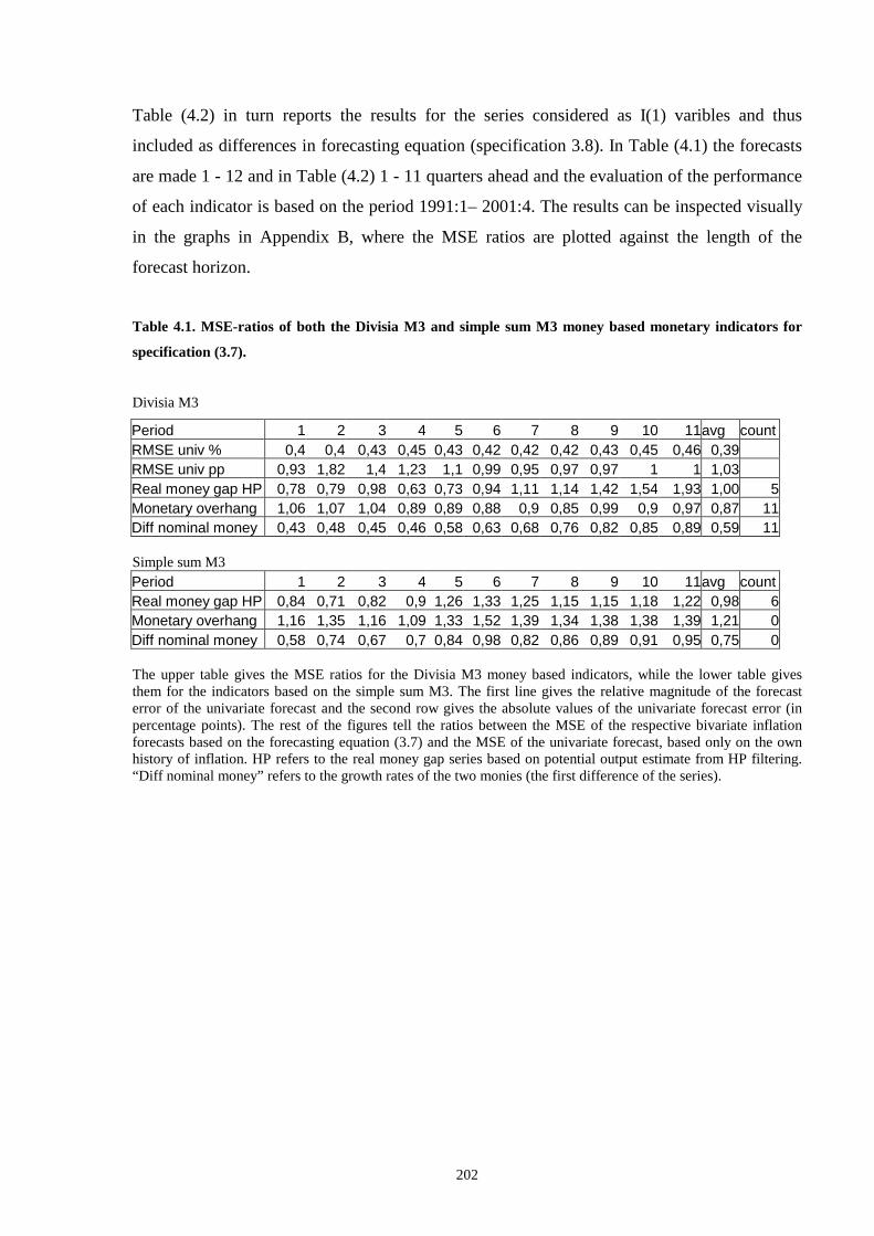
202

Table (4.2) in turn reports the results for the series considered as I(1) varibles and thus

included as differences in forecasting equation (specification 3.8). In Table (4.1) the forecasts

are made 1 - 12 and in Table (4.2) 1 - 11 quarters ahead and the evaluation of the performance

of each indicator is based on the period 1991:1– 2001:4. The results can be inspected visually

in the graphs in Appendix B, where the MSE ratios are plotted against the length of the

forecast horizon.

Table 4.1. MSE-ratios of both the Divisia M3 and simple sum M3 money based monetary indicators for

specification (3.7).

Divisia M3

Period 1 2 3 4 5 6 7 8 9 10 11 avg count RMSE univ % 0,4 0,4 0,43 0,45 0,43 0,42 0,42 0,42 0,43 0,45 0,46 0,39 RMSE univ pp 0,93 1,82 1,4 1,23 1,1 0,99 0,95 0,97 0,97 1 1 1,03 Real money gap HP 0,78 0,79 0,98 0,63 0,73 0,94 1,11 1,14 1,42 1,54 1,93 1,00 5 Monetary overhang 1,06 1,07 1,04 0,89 0,89 0,88 0,9 0,85 0,99 0,9 0,97 0,87 11 Diff nominal money 0,43 0,48 0,45 0,46 0,58 0,63 0,68 0,76 0,82 0,85 0,89 0,59 11 Simple sum M3 Period 1 2 3 4 5 6 7 8 9 10 11 avg count Real money gap HP 0,84 0,71 0,82 0,9 1,26 1,33 1,25 1,15 1,15 1,18 1,22 0,98 6 Monetary overhang 1,16 1,35 1,16 1,09 1,33 1,52 1,39 1,34 1,38 1,38 1,39 1,21 0 Diff nominal money 0,58 0,74 0,67 0,7 0,84 0,98 0,82 0,86 0,89 0,91 0,95 0,75 0 The upper table gives the MSE ratios for the Divisia M3 money based indicators, while the lower table gives them for the indicators based on the simple sum M3. The first line gives the relative magnitude of the forecast error of the univariate forecast and the second row gives the absolute values of the univariate forecast error (in percentage points). The rest of the figures tell the ratios between the MSE of the respective bivariate inflation forecasts based on the forecasting equation (3.7) and the MSE of the univariate forecast, based only on the own history of inflation. HP refers to the real money gap series based on potential output estimate from HP filtering. “Diff nominal money” refers to the growth rates of the two monies (the first difference of the series).

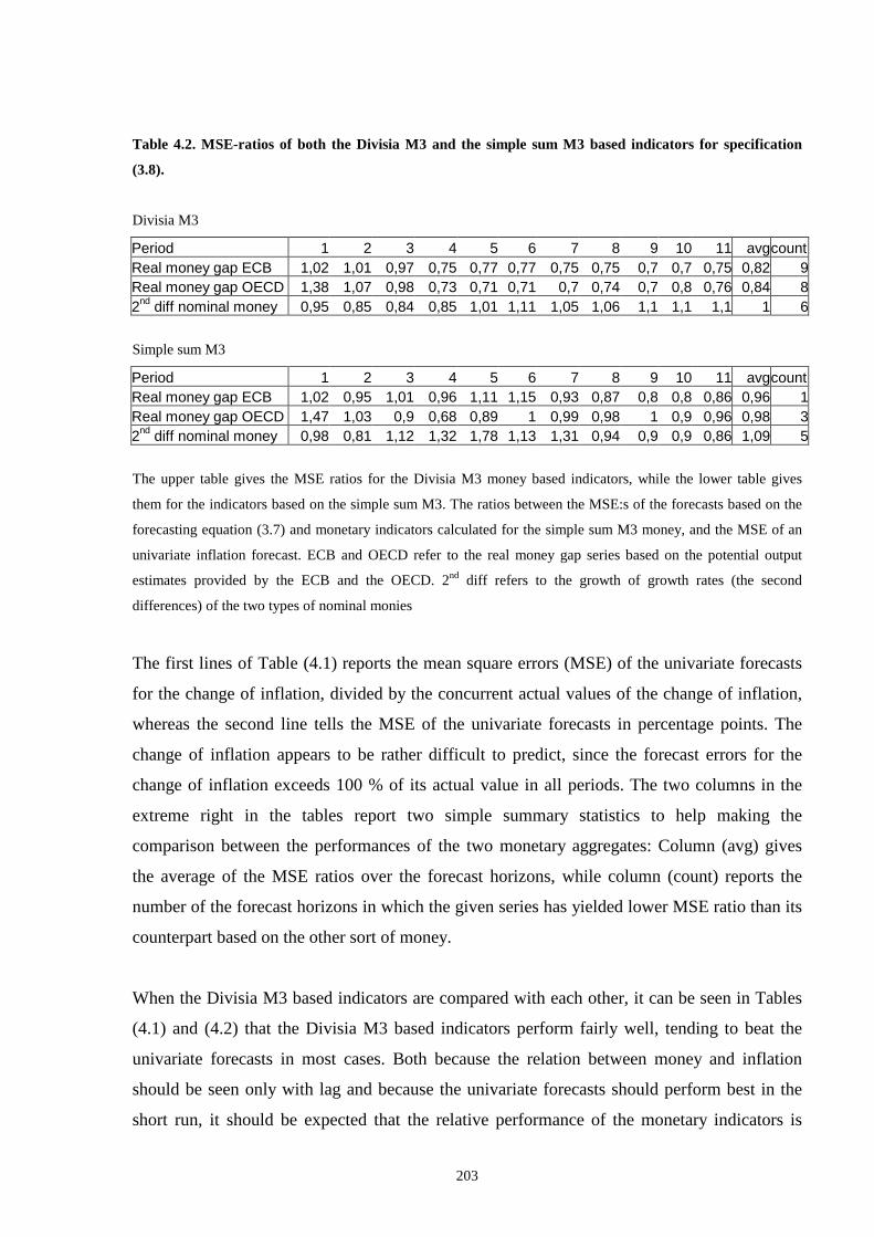
203

Table 4.2. MSE-ratios of both the Divisia M3 and the simple sum M3 based indicators for specification

(3.8).

Divisia M3

Period 1 2 3 4 5 6 7 8 9 10 11 avg count Real money gap ECB 1,02 1,01 0,97 0,75 0,77 0,77 0,75 0,75 0,7 0,7 0,75 0,82 9 Real money gap OECD 1,38 1,07 0,98 0,73 0,71 0,71 0,7 0,74 0,7 0,8 0,76 0,84 8 2nd diff nominal money 0,95 0,85 0,84 0,85 1,01 1,11 1,05 1,06 1,1 1,1 1,1 1 6

Simple sum M3

Period 1 2 3 4 5 6 7 8 9 10 11 avg count Real money gap ECB 1,02 0,95 1,01 0,96 1,11 1,15 0,93 0,87 0,8 0,8 0,86 0,96 1 Real money gap OECD 1,47 1,03 0,9 0,68 0,89 1 0,99 0,98 1 0,9 0,96 0,98 3 2nd diff nominal money 0,98 0,81 1,12 1,32 1,78 1,13 1,31 0,94 0,9 0,9 0,86 1,09 5

The upper table gives the MSE ratios for the Divisia M3 money based indicators, while the lower table gives

them for the indicators based on the simple sum M3. The ratios between the MSE:s of the forecasts based on the

forecasting equation (3.7) and monetary indicators calculated for the simple sum M3 money, and the MSE of an

univariate inflation forecast. ECB and OECD refer to the real money gap series based on the potential output

estimates provided by the ECB and the OECD. 2nd diff refers to the growth of growth rates (the second

differences) of the two types of nominal monies

The first lines of Table (4.1) reports the mean square errors (MSE) of the univariate forecasts

for the change of inflation, divided by the concurrent actual values of the change of inflation,

whereas the second line tells the MSE of the univariate forecasts in percentage points. The

change of inflation appears to be rather diff icult to predict, since the forecast errors for the

change of inflation exceeds 100 % of its actual value in all periods. The two columns in the

extreme right in the tables report two simple summary statistics to help making the

comparison between the performances of the two monetary aggregates: Column (avg) gives

the average of the MSE ratios over the forecast horizons, while column (count) reports the

number of the forecast horizons in which the given series has yielded lower MSE ratio than its

counterpart based on the other sort of money.

When the Divisia M3 based indicators are compared with each other, it can be seen in Tables

(4.1) and (4.2) that the Divisia M3 based indicators perform fairly well , tending to beat the

univariate forecasts in most cases. Both because the relation between money and inflation

should be seen only with lag and because the univariate forecasts should perform best in the

short run, it should be expected that the relative performance of the monetary indicators is

204

increasing in the length of the forecast horizon. This seems, however, not to be the case as is

also shown by the mostly flat or upward sloping graphs of Appendix B. Interestingly, among

all the Divisia money based indicators based on specification (3.7) the best forecasts are

yielded by the growth rate of the nominal Divisia M3 money, even though the series clearly

did not even seem to be stationary. The finding is also interesting in light of the previous

findings by Altimari (2001), Gerlach and Svensson (2001), and Trecroci and Vega (2000) for

the relation between the simple sum M3 money and inflation, since according to these studies

the growth rate of nominal money should be outperformed by the real money gap series. On

the other hand, in Reimers (2002) the growth rates of both the Divisia money and the simple

sum M3 seemed to perform equally as well as the P-star indicator, when the inflation was

defined as GDP inflation. Moreover, all those studies focused on forecasting inflation itself

rather than changes in it as it is the case in the paper at hand. For specification (3.8) the best

forecasts are yielded by the real money gap series based on the ECB estimate of the potential

output.

Turning next to comparing the simple sum indicators with each other, it can be seen in the

tables that now the univariate forecasts more often have outperformed the monetary indicators.

The best forecasts in specification (3.7) are in fact again given by the growth rate of nominal

money, while bothe the real money gap series based on the HP-filter based estimate of the

potential output and the monetary overhang are mostly outperformed even by the univariate

inflation forecasts. Among the forecasts based on the specification (3.8) the real money gap

based on the potential output estimated by the ECB and OECD seem, however, perform better

than the the “growth of the growth rate” of the nominal simple sum M3 money.

Overall comparison between the forecasting performance of the Divisia M3 based indicators

and the indicators based on the simple sum M3 suggests that the Divisia money indicators

slightly outperform their simple sum M3 counterparts. The conclusion is supported both by

the average MSE ratios and the number of forecast horizons in which the Divisia M3

indicators are assigned lower MSE ratios than their simple sum M3 counterparts. The Divisia

money based indicators yield better forecasts in cases of the monetary overhang and the real

money gaps based on the potential output estimates provided by the ECB and the OECD. The

difference in favour of the Divisia money based indicators does not seem to be large, however.

The cases of the second difference of the nominal M3 monies and the real money gap series

based on potential output estimates from HP-filtering, in turn, seem unclear, regardless of

205

which of our two criteria to assess the relative performance of the indicators is applied18. As it

was previously noted, the Divisia money is expected to contain more information about future

inflation especially in the short run, while in the long run the forecasts are likely to converge.

This pattern is, however, not seen in the results. Except the case of the growth rates of the

nominal monies, the difference in the forecast performance in favor of the Divisia money

indicators does not seem to be notably larger in the short end than in the long end of the

foreast horzons.19

Interestingly, the growth rate of the nominal Divisia M3 not only beats the othe Divisia M3

based indicators but also yields the best forecasts among all the different monetary indicators

considered. In horizons between one and four quarters, the forecast MSE:s of the growth rate

of the nominal Divisia money remains below 50 % of the MSE of the univariate forecast. It is

notable that the growth rate of the simple sum M3 money, the ECB’s actual “ target variable”,

also performs fairly well , although remains outperformed by its Divisia money counterpart in

every forecast horizon.

5. CONCLUSIONS

The ECB has given the M3 monetary aggregate an important role as an indicator variable for

the future inflation in the euro area. This study has discussed, whether the synthetic Divisia

M3 monetary aggregate, computed as a weighted average of its component assets, could

provide more information on the future price developments than the ordinary M3 aggregate,

which does not take into account the differing degrees of liquidity of the component assets of

the aggregate. Although in the long run the predictions based on the two aggregates are likely

to converge, it is a priori assumed that the Divisia money may yield more accurate forecasts in

the short-run. As an econometric method I have used simulated out-of-sample forecasting. The

study differs from the previous studies on the information content of the Divisia money on the

euro area inflation in that here inflation is assumed as I(1) variable and thus the change in

inflation, rather than inflation itself, has been the variable to be forecasted. In addition to

18 The forecasting performance of the HP-filter based real money gap series for the simple sum money was in fact significantly improved when it was included in the forecast equation in differences, using specification (3.8). The relative performance between the HP-filter based real money gap series for the two monies remained unclear, however.

206

comparing the forecasting performance of the growth rates of the two nominal M3 monies, the

study has focused on the performance of the real money gap and the monetary overhang

variables calculated for the two types of monies.

It was found, firstly, that some of the monetary indicator series based on the synthetic Divisia

M3 monetary aggregate really improved the out-of-sample forecasts for the (change in) the

euro area inflation, when compared to the forecasts based on simple univariate forecasts.

Secondly, comparison between the forecasting performance of the different monetary

indicator series calculated for our two sort of monetary aggregates revealed that the Divisia

money based indicators tend to outperform their simple sum money based counterparts at least

in some cases.

It was also an interesting finding that the growth rate of the nominal Divisia money seemed to

perform surprisingly well , even though the growth rates of both type of nominal monies were

considered non-stationary variables and although it was the change in inflation rather than

inflation itself that was to be forecasted. The growth rate of the Divisia money yielded the best

forecasts not only within the Divisia money based indicators but it also outperformed the

simple sum M3 based indicators. The finding contradicts the previous findings based on the

simple sum M3 money, according to which real money gap and money overhang – variables

that measure the gap between the desired and actual level of real money holdings, suit best for

the forecasting purposes. From a theoretical perspective, the performance of the growth rate of

the Divisia money is even more interesting, when taking into account the recent arguments

according to which the estimations based on simple linear regressions in fact understate the

relations between money and inflation, since this relation is probably too subtle to be revealed

by a simple linear one-equation model20.

All i n all , the results support the previous findings by Stracca (2001) and Reimers (2002),

according to which the synthetic Divisia M3 monetary aggregate could play a role as a

valuable indicator variable on the future price developments in the euro area, at least when

used along with the ordinary, simple sum monetary aggregates. A longer inflation history will

be needed, however, to ascertain whether it is the growth rate of the nominal Divisia money or

19 In fact, e.g. the “growth of growth rate” of the Divisia M3 also yields better forecasts in short horizons, but at the long end of the forecasts the simple sum M3 indicators now perform significantly better. 20 See eg King (2002)

207

some Divisia money based measure for the excess liquidity in the economy, that the ECB

should actually be looking at.

Some caution is needed in interpreting the results, however. Firstly, because the study is based

on aggregated euro area wide data, all the relations between money and prices that the study

suggests represent averages of these relations over the EMU member countries. Most of the

time in the sample period, the transmission process between money and prices has been based

on independent monetary policies in the member states, however. The average of these

transmission processes may differ from the transmission process under the regime of common

monetary policy, which may also have caused a structural shift in the relation between money

and prices. Secondly, in the end of the sample period there might have occurred pure portfolio

shift in the money demand, due to changes in the opportunity costs of holding money. This

portfolio shift may in its part have obscured the link between money and inflation during the

sample period. Thirdly, the relatively short sample period and some obvious structural breaks

in the period resulted in some uncertainties concerning the time series properties of both the

euro area inflation and the monetary indicator series.

208

REFERENCES

Allsopp, C.

The Future of Macroeconomic Policy in the European Union

Speech to the Austrian Institute of Economic Research (WIFO), 23 January 2002.

Altimari, S. N. (2001)

Does Money Lead Inflation in the Euro Ar ea?

ECB Working Paper N:o 63.

Barnett, W. A. (1980)

Economic Monetary Aggregates: An Application of Index Number and Application

Theory”

Journal of Econometrics, 14, pp. 11 – 18.

Barnett, W. A. (2000)

Understanding the New Divisia Monetary Aggregates

In “The Theory of Monetary Aggregation” , edited by Barnett, W. A. and Serletis, A.

North Holland.

Brand, C. – Cassola, N. (2000)

A Money Demand System for Euro Area M3

ECB Working Paper series N:o 39.

Calza, A. – Gerdesmeier, D. – Levy, J. (2001)

Euro Area Money Demand: Measur ing the Opportunity Cost Appropr iately

IMF Working Paper N:o 179.

Coenen, G. – Vega, J. L. (1999)

The Demand for M 3 in the Euro Area

ECB Working Paper series 6.

209

De Grauwe, P. – Polan M. (2001)

Is Inflation Always and Everywhere a Monetary Phenomenon?

Manuscript. CEPR and University of Leuven.

Dorsey, R. E. (2000)

Neural Networks with Divisia Money: Better Forecasts of Future Inflation?

In “Divisia Monetary Aggregates” , edited by Belongia M. T. and Binner, J. M.

Palgrave.

Fagan, G. – Henry, J. (1998)

Long run money demand in the EU: Evidence for area-wide aggregates

Empirical Economics 23: pp. 483 – 506.

Gerlach, S. – Svensson, L.E.O. (2001)

Money and inflation in the Euro Area: A case for monetary indicators?

BIS Working Papers N:o 98.

Juselius, K. (1999)

Models and Relations in Economics and Econometr ics

Journal of Economic Methodology, Vol 6, p. 259 – 290.

Juselius, K. – McDonald R. (2000)

International Par ity Relationships between Germany and the United States: A Joint

Modeling Approach.

An unpublished mimeo.

King, M. (2002) No money, no inflation – the role of money in the economy The Bank of England Quarterly Bulletin, Summer 2002.

Kontolemis, Z. G. (2000)

Money Demand in the Euro Area: Where Do We Stand (Today)?

IMF Working Paper 185 / 2002.

210

Kontolemis, Z. G. (2002)

Interest Rates in the Euro Area: Modeling the ECB’s Reaction Function.

Unpublished mimeo.

Masuch, K. – Pill , H. – Will eke, C.

Framework and tools of monetary analysis

In “Monetary Analysis: Tools and Applications” , edited by Klockers, H.-J. and Will eke, C.

ECB 2001.

McKinnon, J. G. (1991)

Critical Values for Cointegration Tests

In "Long-Run Economic Relationships” , edited by Engle and Granger, 1991.

Meltzer, A. H. (1999) The transmission process Mimeo, Carnegie Mellon University.

Meltzer, A. H. (2001)

Money and Monetary Policy: An Essay in Honor of Darr yl Francis

Federal Reserve Bank of St. Louis Review, July/August 2001.

Nelson, E. (2002) Direct effects of base money on aggregate demand: theory and evidence Journal of Monetary Economics, Vol. 49:4. May 2002, Pages 687-708.

Reimers, H.-E. (2002)

Analysing Divisia Aggregates for the Euro Area.

Economic Research Centre of the Deutsche Bundesbank. Discussion Paper 13/02.

Seitz, F. and Tödter, K.-H. (2001)

How the P* Model Rationalises Monetary Targeting - A Comment on Svensson

German Economic Review 2 (2001) p.303-308.

(Downloadable on http://www.princeton.edu/~svensson/)

211

Stracca, L. (2001)

Does L iquidity Matter? Properties of a Synthetic Divisia Monetary Aggregate in the

Euro Area

ECB Working Paper Series N:o 79.

Stracca, L. (2001b)

The Functional Form of the Euro Area Demand for M 1

ECB Working Paper series N:o 51.

Stock, J. H. – Watson, M. W. (1999)

Forecasting inflation

Journal of Monetary Economics 44, p. 293 – 335.

Svensson, L. E. O. (1999)

Does the *P Model Provide Any Rationale for M onetary Targeting?

German Economic Review 1, February 2000, p. 69-81

(Downloadable on http://www.princeton.edu/~svensson/)

Trecroci, C. – Vega, J. L. (2000)

The information content of M3 for future inflation

ECB Working Papers N:o 33.

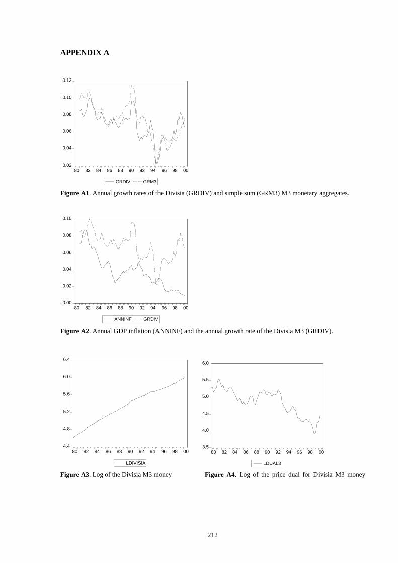
212

APPENDIX A

0.02

0.04

0.06

0.08

0.10

0.12

80 82 84 86 88 90 92 94 96 98 00

GRDIV GRM3

Figure A1. Annual growth rates of the Divisia (GRDIV) and simple sum (GRM3) M3 monetary aggregates.

0.00

0.02

0.04

0.06

0.08

0.10

80 82 84 86 88 90 92 94 96 98 00

ANNINF GRDIV

Figure A2. Annual GDP inflation (ANNINF) and the annual growth rate of the Divisia M3 (GRDIV).

4.4

4.8

5.2

5.6

6.0

6.4

80 82 84 86 88 90 92 94 96 98 00

LDIVISIA

3.5

4.0

4.5

5.0

5.5

6.0

80 82 84 86 88 90 92 94 96 98 00

LDUAL3

Figure A3. Log of the Divisia M3 money Figure A4. Log of the price dual for Divisia M3 money

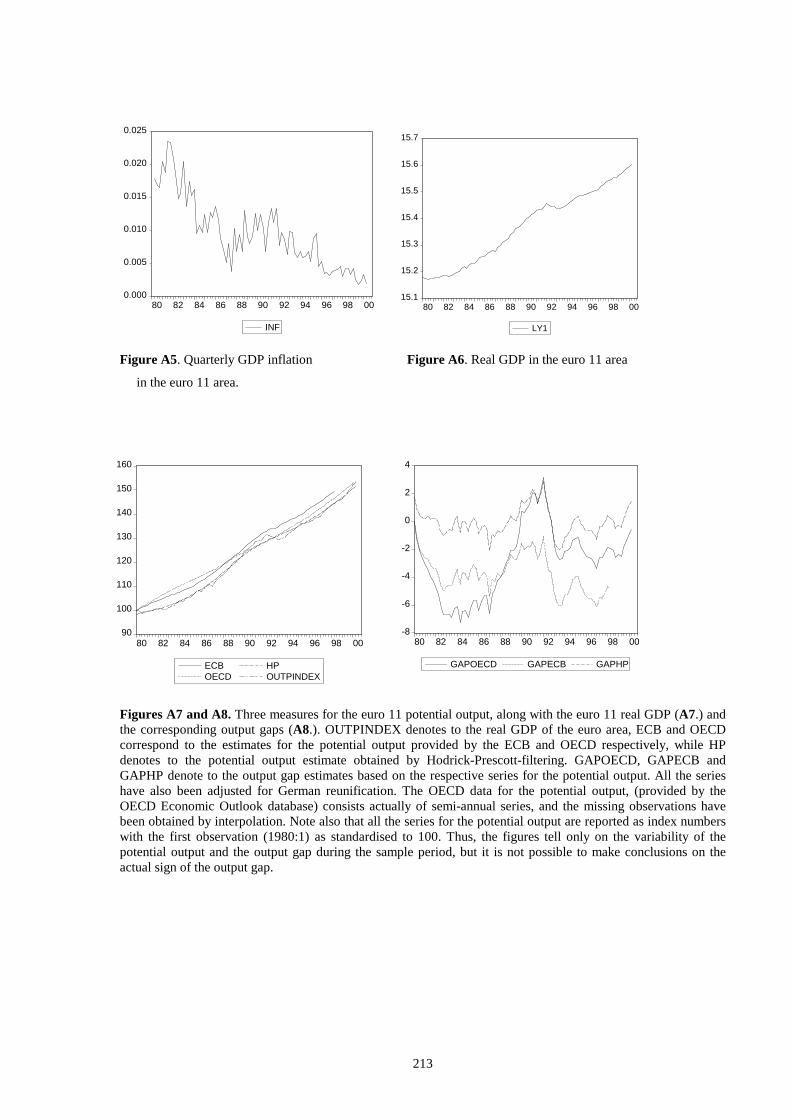
213

0.000

0.005

0.010

0.015

0.020

0.025

80 82 84 86 88 90 92 94 96 98 00

INF

15.1

15.2

15.3

15.4

15.5

15.6

15.7

80 82 84 86 88 90 92 94 96 98 00

LY1

Figure A5. Quarterly GDP inflation Figure A6. Real GDP in the euro 11 area

in the euro 11 area.

Figures A7 and A8. Three measures for the euro 11 potential output, along with the euro 11 real GDP (A7.) and the corresponding output gaps (A8.). OUTPINDEX denotes to the real GDP of the euro area, ECB and OECD correspond to the estimates for the potential output provided by the ECB and OECD respectively, while HP denotes to the potential output estimate obtained by Hodrick-Prescott-filtering. GAPOECD, GAPECB and GAPHP denote to the output gap estimates based on the respective series for the potential output. All the series have also been adjusted for German reunification. The OECD data for the potential output, (provided by the OECD Economic Outlook database) consists actually of semi-annual series, and the missing observations have been obtained by interpolation. Note also that all the series for the potential output are reported as index numbers with the first observation (1980:1) as standardised to 100. Thus, the figures tell only on the variabilit y of the potential output and the output gap during the sample period, but it is not possible to make conclusions on the actual sign of the output gap.

-8

-6

-4

-2

0

2

4

80 82 84 86 88 90 92 94 96 98 00

GAPOECD GAPECB GAPHP

90

100

110

120

130

140

150

160

80 82 84 86 88 90 92 94 96 98 00

ECBOECD

HPOUTPINDEX

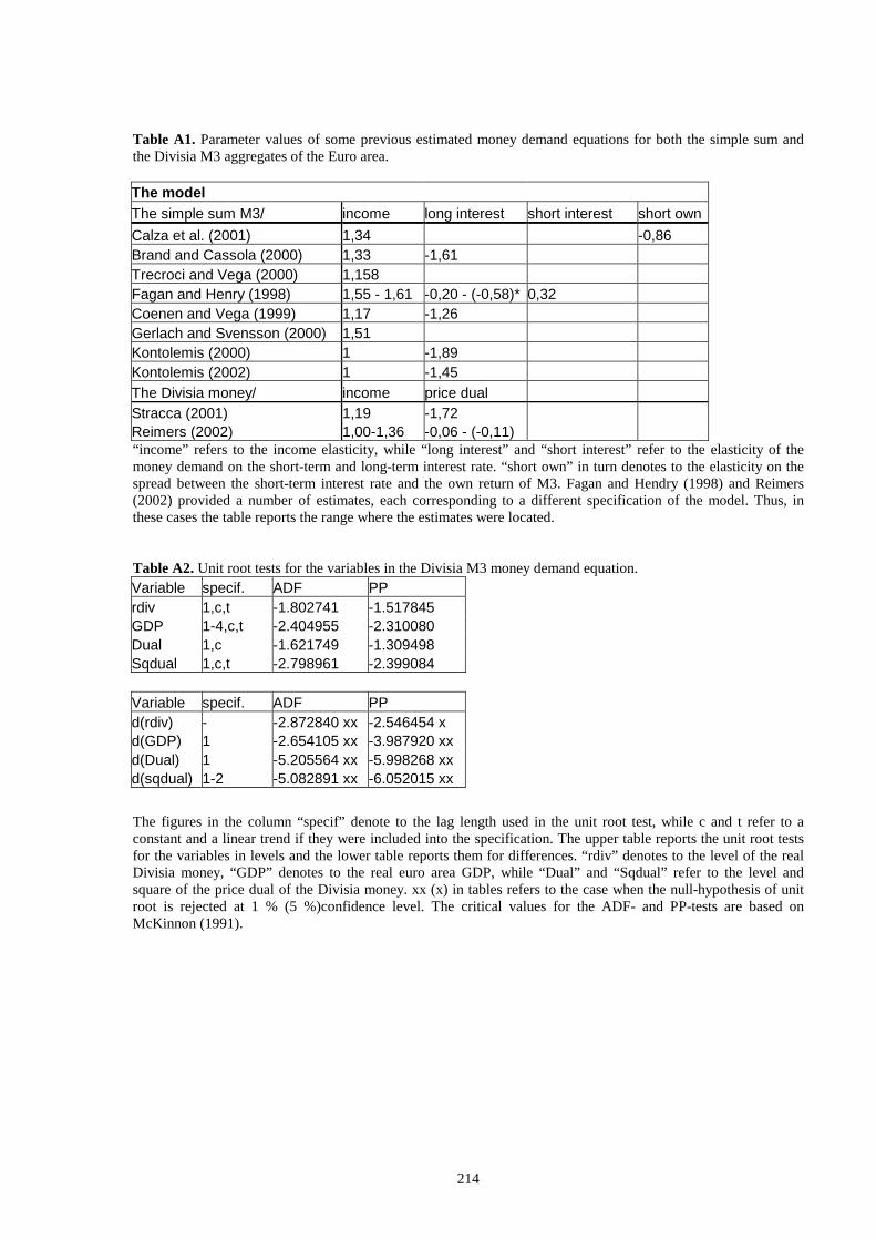
214

Table A1. Parameter values of some previous estimated money demand equations for both the simple sum and the Divisia M3 aggregates of the Euro area. The model The simple sum M3/ income long interest short interest short own

Calza et al. (2001) 1,34 -0,86 Brand and Cassola (2000) 1,33 -1,61 Trecroci and Vega (2000) 1,158 Fagan and Henry (1998) 1,55 - 1,61 -0,20 - (-0,58)* 0,32 Coenen and Vega (1999) 1,17 -1,26 Gerlach and Svensson (2000) 1,51 Kontolemis (2000) 1 -1,89 Kontolemis (2002) 1 -1,45 The Divisia money/ income price dual Stracca (2001) 1,19 -1,72 Reimers (2002) 1,00-1,36 -0,06 - (-0,11) “ income” refers to the income elasticity, while “ long interest” and “short interest” refer to the elasticity of the money demand on the short-term and long-term interest rate. “short own” in turn denotes to the elasticity on the spread between the short-term interest rate and the own return of M3. Fagan and Hendry (1998) and Reimers (2002) provided a number of estimates, each corresponding to a different specification of the model. Thus, in these cases the table reports the range where the estimates were located. Table A2. Unit root tests for the variables in the Divisia M3 money demand equation. Variable specif. ADF PP rdiv 1,c,t -1.802741 -1.517845 GDP 1-4,c,t -2.404955 -2.310080 Dual 1,c -1.621749 -1.309498 Sqdual 1,c,t -2.798961 -2.399084 Variable specif. ADF PP d(rdiv) - -2.872840 xx -2.546454 x d(GDP) 1 -2.654105 xx -3.987920 xx d(Dual) 1 -5.205564 xx -5.998268 xx d(sqdual) 1-2 -5.082891 xx -6.052015 xx

The figures in the column “specif” denote to the lag length used in the unit root test, while c and t refer to a constant and a linear trend if they were included into the specification. The upper table reports the unit root tests for the variables in levels and the lower table reports them for differences. “ rdiv” denotes to the level of the real Divisia money, “GDP” denotes to the real euro area GDP, while “Dual” and “Sqdual” refer to the level and square of the price dual of the Divisia money. xx (x) in tables refers to the case when the null -hypothesis of unit root is rejected at 1 % (5 %)confidence level. The critical values for the ADF- and PP-tests are based on McKinnon (1991).

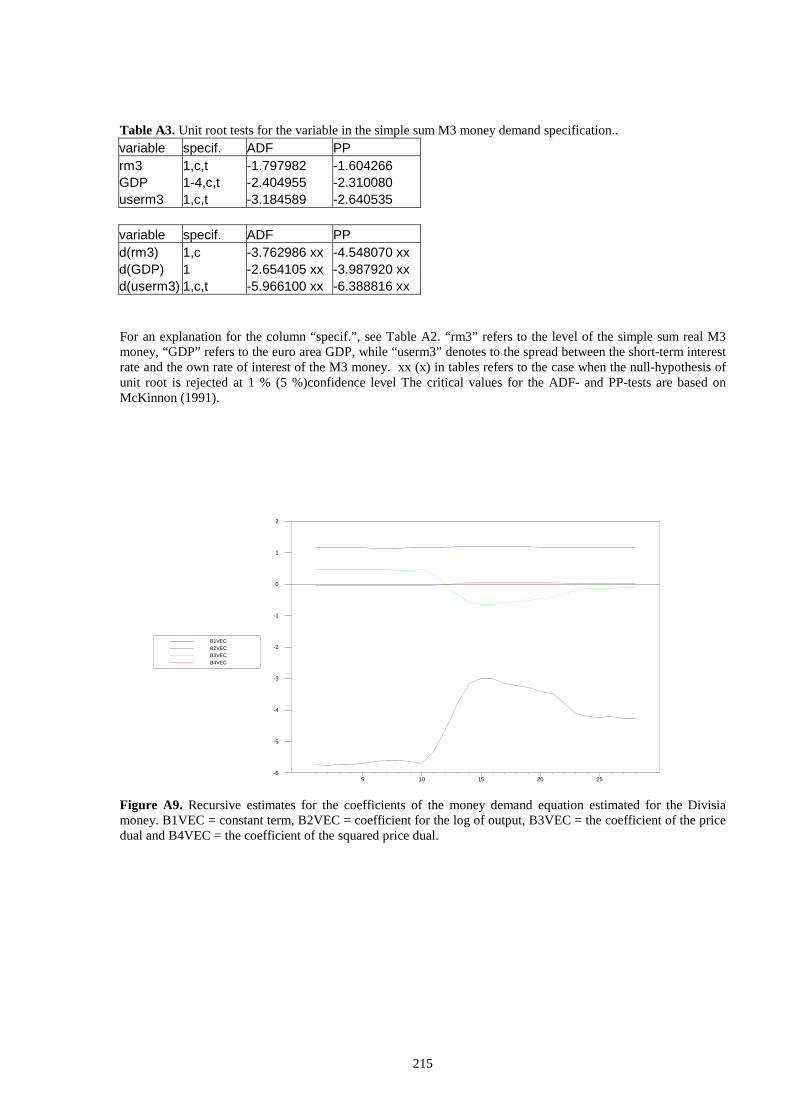
215

Table A3. Unit root tests for the variable in the simple sum M3 money demand specification.. variable specif. ADF PP rm3 1,c,t -1.797982 -1.604266 GDP 1-4,c,t -2.404955 -2.310080 userm3 1,c,t -3.184589 -2.640535 variable specif. ADF PP d(rm3) 1,c -3.762986 xx -4.548070 xx d(GDP) 1 -2.654105 xx -3.987920 xx d(userm3) 1,c,t -5.966100 xx -6.388816 xx

For an explanation for the column “specif.” , see Table A2. “ rm3” refers to the level of the simple sum real M3 money, “GDP” refers to the euro area GDP, while “userm3” denotes to the spread between the short-term interest rate and the own rate of interest of the M3 money. xx (x) in tables refers to the case when the null -hypothesis of unit root is rejected at 1 % (5 %)confidence level The critical values for the ADF- and PP-tests are based on McKinnon (1991).

Figure A9. Recursive estimates for the coeff icients of the money demand equation estimated for the Divisia money. B1VEC = constant term, B2VEC = coeff icient for the log of output, B3VEC = the coeff icient of the price dual and B4VEC = the coeff icient of the squared price dual.

B1VECB2VECB3VECB4VEC

5 10 15 20 25-6

-5

-4

-3

-2

-1

0

1

2

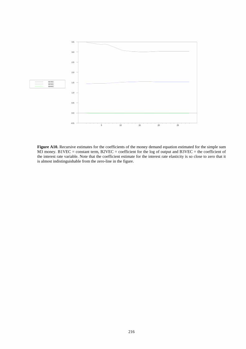
216

Figure A10. Recursive estimates for the coeff icients of the money demand equation estimated for the simple sum M3 money. B1VEC = constant term, B2VEC = coeff icient for the log of output and B3VEC = the coeff icient of the interest rate variable. Note that the coeff icient estimate for the interest rate elasticity is so close to zero that it is almost indistinguishable from the zero-line in the figure.

B1VECB2VECB3VEC

5 10 15 20 25-0.5

0.0

0.5

1.0

1.5

2.0

2.5

3.0

3.5

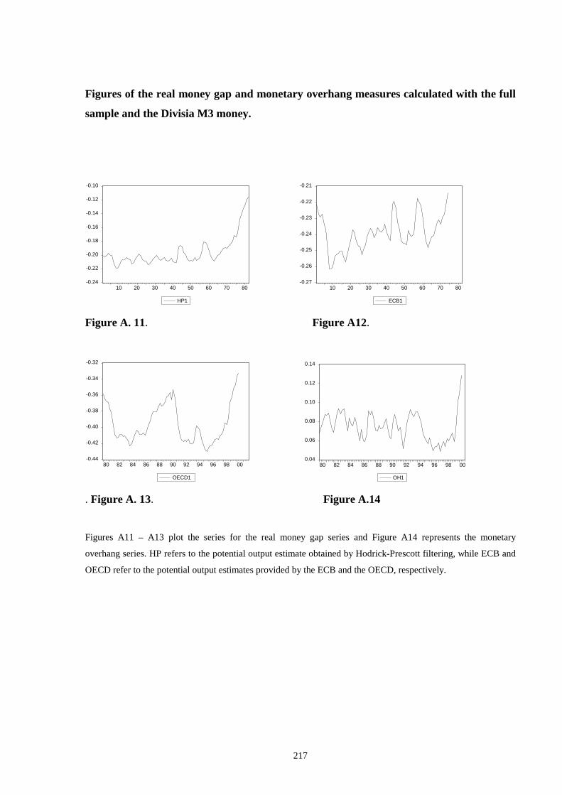
217

Figures of the real money gap and monetary overhang measures calculated with the full

sample and the Divisia M3 money.

-0.24

-0.22

-0.20

-0.18

-0.16

-0.14

-0.12

-0.10

10 20 30 40 50 60 70 80

HP1

-0.27

-0.26

-0.25

-0.24

-0.23

-0.22

-0.21

10 20 30 40 50 60 70 80

ECB1

Figure A. 11. Figure A12.

-0.44

-0.42

-0.40

-0.38

-0.36

-0.34

-0.32

80 82 84 86 88 90 92 94 96 98 00

OECD1

0.04

0.06

0.08

0.10

0.12

0.14

80 82 84 86 88 90 92 94 96 98 00

OH1

. Figure A. 13. Figure A.14

Figures A11 – A13 plot the series for the real money gap series and Figure A14 represents the monetary

overhang series. HP refers to the potential output estimate obtained by Hodrick-Prescott filtering, while ECB and

OECD refer to the potential output estimates provided by the ECB and the OECD, respectively.

218

Figures of the real money gap and monetary overhang measures calculated with the full

sample and the simple sum M3 money.

Figure A. 15 Figure A. 16

Figure A.17 Figure A. 18

Figures A15 – A17 plot the series for the real money gap series and Figure A18 represents the monetary

overhang series. HP refers to the potential output estimate obtained by Hodrick-Prescott filtering, while ECB and

OECD refer to the potential output estimates provided by the ECB and the OECD, respectively.

0.01

0.02

0.03

0.04

0.05

0.06

0.07

80 82 84 86 88 90 92 94 96 98 00

HP1M3

-0.04

-0.03

-0.02

-0.01

0.00

0.01

0.02

80 82 84 86 88 90 92 94 96 98 00

ECB1M3

-0.04

-0.02

0.00

0.02

0.04

0.06

80 82 84 86 88 90 92 94 96 98 00

OH1M3B

-0.06

-0.04

-0.02

0.00

0.02

0.04

0.06

0.08

80 82 84 86 88 90 92 94 96 98 00

OECD1M3

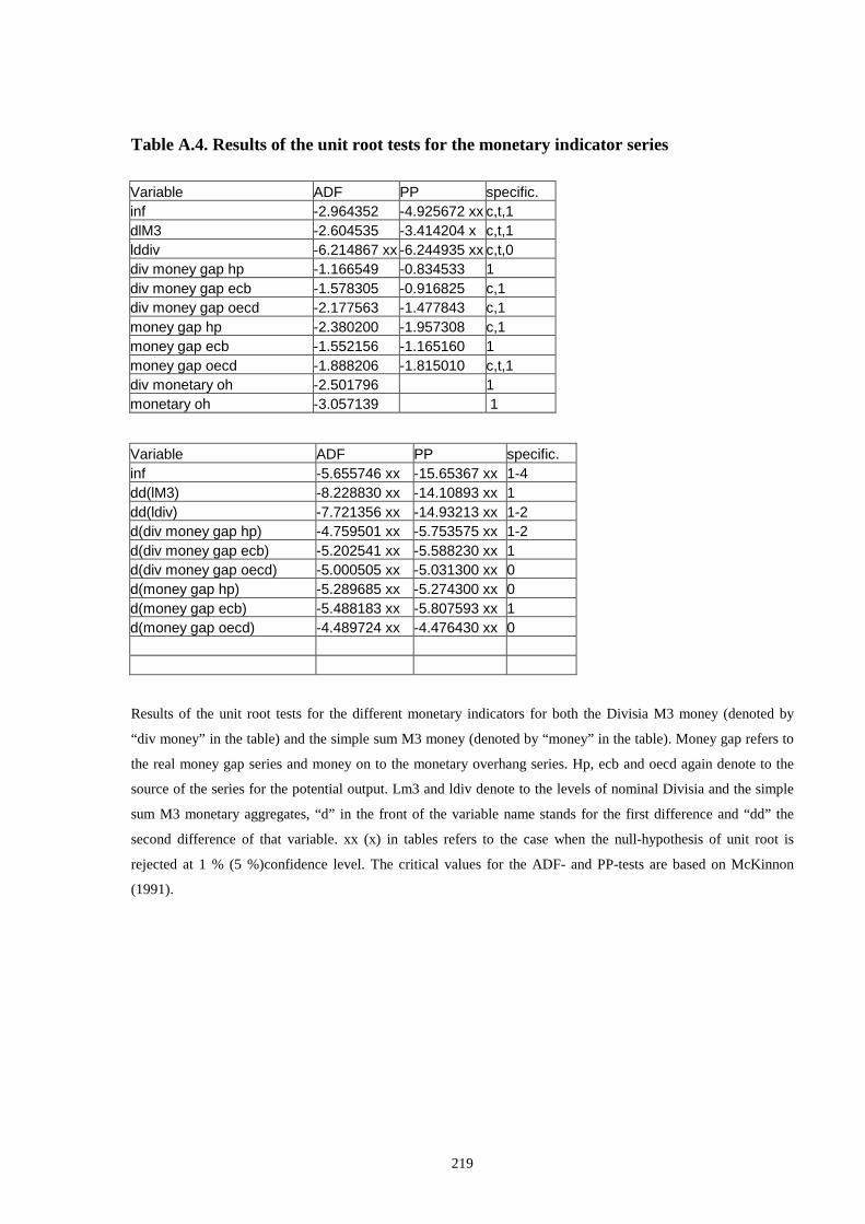
219

Table A.4. Results of the unit root tests for the monetary indicator series

Variable ADF PP specific. inf -2.964352 -4.925672 xx c,t,1 dlM3 -2.604535 -3.414204 x c,t,1 lddiv -6.214867 xx -6.244935 xx c,t,0 div money gap hp -1.166549 -0.834533 1 div money gap ecb -1.578305 -0.916825 c,1 div money gap oecd -2.177563 -1.477843 c,1 money gap hp -2.380200 -1.957308 c,1 money gap ecb -1.552156 -1.165160 1 money gap oecd -1.888206 -1.815010 c,t,1 div monetary oh -2.501796 1 monetary oh -3.057139 1

Variable ADF PP specific. inf -5.655746 xx -15.65367 xx 1-4 dd(lM3) -8.228830 xx -14.10893 xx 1 dd(ldiv) -7.721356 xx -14.93213 xx 1-2 d(div money gap hp) -4.759501 xx -5.753575 xx 1-2 d(div money gap ecb) -5.202541 xx -5.588230 xx 1 d(div money gap oecd) -5.000505 xx -5.031300 xx 0 d(money gap hp) -5.289685 xx -5.274300 xx 0 d(money gap ecb) -5.488183 xx -5.807593 xx 1 d(money gap oecd) -4.489724 xx -4.476430 xx 0

Results of the unit root tests for the different monetary indicators for both the Divisia M3 money (denoted by

“div money” in the table) and the simple sum M3 money (denoted by “money” in the table). Money gap refers to

the real money gap series and money on to the monetary overhang series. Hp, ecb and oecd again denote to the

source of the series for the potential output. Lm3 and ldiv denote to the levels of nominal Divisia and the simple

sum M3 monetary aggregates, “d” in the front of the variable name stands for the first difference and “dd” the

second difference of that variable. xx (x) in tables refers to the case when the null -hypothesis of unit root is

rejected at 1 % (5 %)confidence level. The critical values for the ADF- and PP-tests are based on McKinnon

(1991).

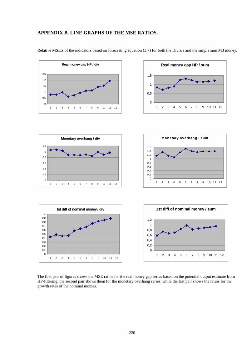
220

APPENDIX B. L INE GRAPHS OF THE MSE RATIOS.

Relative MSE:s of the indicators based on forecasting equation (3.7) for both the Divisia and the simple sum M3 money.

The first pair of figures shows the MSE ratios for the real money gap series based on the potential output estimate from HP-filtering, the second pair shows them for the monetary overhang series, while the last pair shows the ratios for the growth rates of the nominal monies.

Real money gap HP / sum

0

0,5

1

1,5

1 2 3 4 5 6 7 8 9 10 11 12

Real money gap HP / div

0

0,5

1

1,5

2

2,5

1 2 3 4 5 6 7 8 9 10 11 12

Monetary overhang / div

0

0,2

0,4

0,6

0,8

1

1,2

1 2 3 4 5 6 7 8 9 10 11 12

M onetary overhang / sum

0

0,2

0,4

0,6

0,8

1

1,2

1,4

1,6

1 2 3 4 5 6 7 8 9 10 11 12

!st diff of nominal money / div

0

0,1

0,2

0,3

0,4

0,5

0,6

0,7

0,8

0,9

1

1 2 3 4 5 6 7 8 9 10 11 12

1st diff of nominal money / sum

0

0,2

0,4

0,6

0,8

1

1,2

1 2 3 4 5 6 7 8 9 10 11 12

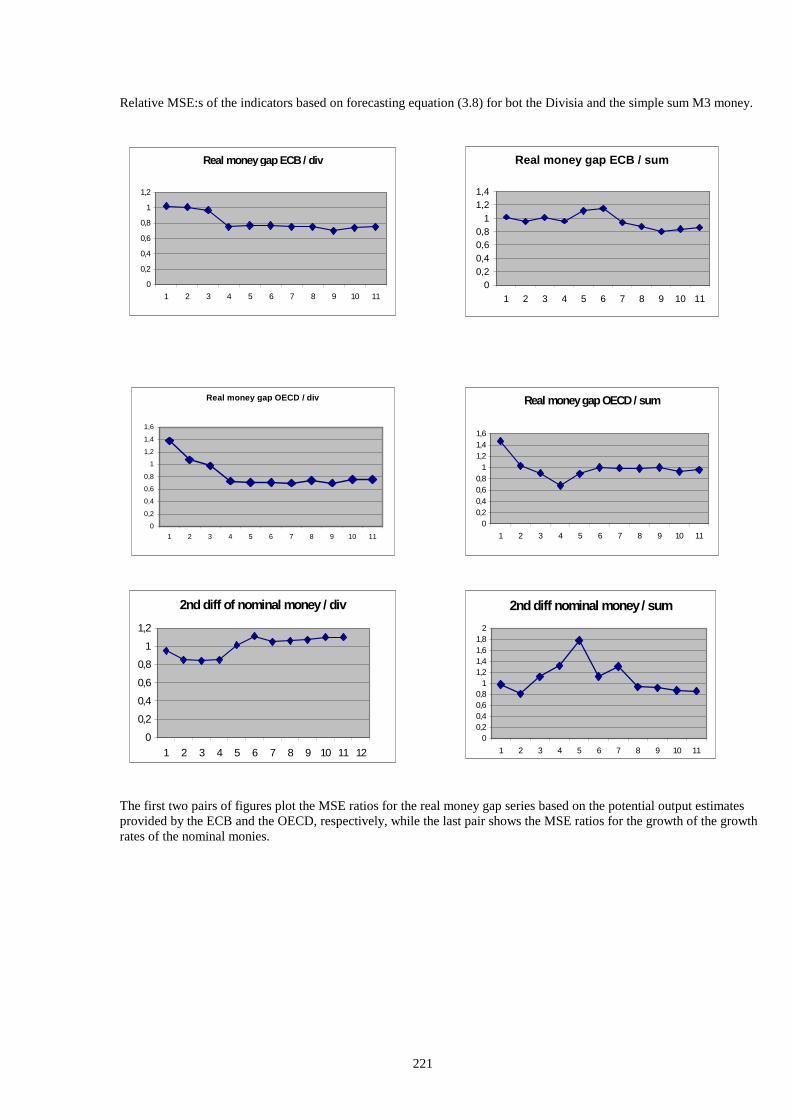
221

Relative MSE:s of the indicators based on forecasting equation (3.8) for bot the Divisia and the simple sum M3 money.

The first two pairs of figures plot the MSE ratios for the real money gap series based on the potential output estimates provided by the ECB and the OECD, respectively, while the last pair shows the MSE ratios for the growth of the growth rates of the nominal monies.

Real money gap ECB / div

0

0,2

0,4

0,6

0,8

1

1,2

1 2 3 4 5 6 7 8 9 10 11

Real money gap ECB / sum

00,20,40,60,8

11,21,4

1 2 3 4 5 6 7 8 9 10 11

Real money gap OECD / div

0

0,2

0,4

0,6

0,8

1

1,2

1,4

1,6

1 2 3 4 5 6 7 8 9 10 11

Real money gap OECD / sum

00,20,40,60,8

11,21,41,6

1 2 3 4 5 6 7 8 9 10 11

2nd diff of nominal money / div

0

0,2

0,4

0,6

0,8

1

1,2

1 2 3 4 5 6 7 8 9 10 11 12

2nd diff nominal money / sum

00,20,40,60,8

11,21,41,61,8

2

1 2 3 4 5 6 7 8 9 10 11