Essays in Financial Economics - dash.harvard.edu

Essays in Financial EconomicsThe Harvard community has made this

article openly available. Please share howthis access benefits you. Your story matters

Citation Kruger, Samuel Arthur. 2014. Essays in Financial Economics.Doctoral dissertation, Harvard University.

Citable link http://nrs.harvard.edu/urn-3:HUL.InstRepos:12274602

Terms of Use This article was downloaded from Harvard University’s DASHrepository, and is made available under the terms and conditionsapplicable to Other Posted Material, as set forth at http://nrs.harvard.edu/urn-3:HUL.InstRepos:dash.current.terms-of-use#LAA

http://osc.hul.harvard.edu/dash/open-access-feedback?handle=&title=Essays%20in%20Financial%20Economics&community=1/1&collection=1/4927603&owningCollection1/4927603&harvardAuthors=e407434630f49fa4e919ae44025af61f&department

http://nrs.harvard.edu/urn-3:HUL.InstRepos:12274602

http://nrs.harvard.edu/urn-3:HUL.InstRepos:dash.current.terms-of-use#LAA



Essays in Financial Economics

A dissertation presented

by

Samuel Arthur Kruger

to

The Department of Business Economics

in partial fulfillment of the requirements

for the degree of

Doctor of Philosophy

in the subject of

Business Economics

Harvard University

Cambridge, Massachusetts

April 2014

c© 2014 Samuel Arthur Kruger

All rights reserved.

Dissertation Advisor:Professor John Y. Campbell

Author:Samuel Arthur Kruger

Essays in Financial Economics

Abstract

This dissertation consists of three independent essays. Chapter 1, “The Effect of Mortgage

Securitization on Foreclosure and Modification,” assesses the impact of mortgage securi-

tization on foreclosure and modification. My primary innovation is using the freeze of

private mortgage securitization in the third quarter of 2007 to instrument for the probability

that a loan is securitized. I find that privately securitized mortgages are substantially

more likely to be foreclosed and less likely to be modified. Chapter 2, “Disagreement and

Liquidity,” analyzes how disagreement between investors affects the relationship between

trading, liquidity, and asymmetric information. Traditional models predict that asymmetric

information should destroy trade and liquidity. In contrast, I document empirical evidence

that asymmetric information increases trading volumes in stock, corporate bond, and option

markets. To resolve this puzzle, I propose a model of overconfident disagreement trading in

which private information enhances trading and liquidity. Chapter 3, “Is Real Interest Rate

Risk Priced? Theory and Empirical Evidence," asks whether investors demand compensation

for holding assets whose returns covary with real interest rate shocks. Empirically, there is

little evidence that real interest rate risk is priced in the cross section of stocks or across asset

classes. Theoretically, interest rate risk can be positively or negatively priced depending on

whether interest rate changes are due to time preference shocks or consumption growth

shocks.

iii

Contents

Abstract . . . . . . . . . . . . . . . . . . . . . . . . . . . . . . . . . . . . . . . . . . . . iiiAcknowledgments . . . . . . . . . . . . . . . . . . . . . . . . . . . . . . . . . . . . . ix

1 The Effect of Mortgage Securitization on Foreclosure and Modification 11.1 Introduction . . . . . . . . . . . . . . . . . . . . . . . . . . . . . . . . . . . . . . 11.2 Existing Evidence . . . . . . . . . . . . . . . . . . . . . . . . . . . . . . . . . . . 41.3 Data and Methodology . . . . . . . . . . . . . . . . . . . . . . . . . . . . . . . . 8

1.3.1 Loan Performance Data . . . . . . . . . . . . . . . . . . . . . . . . . . . 81.3.2 Instrumental Variables Methodology . . . . . . . . . . . . . . . . . . . 11

1.4 Results . . . . . . . . . . . . . . . . . . . . . . . . . . . . . . . . . . . . . . . . . 211.4.1 Baseline Results . . . . . . . . . . . . . . . . . . . . . . . . . . . . . . . . 211.4.2 Interpreting the Results . . . . . . . . . . . . . . . . . . . . . . . . . . . 251.4.3 Robustness Checks . . . . . . . . . . . . . . . . . . . . . . . . . . . . . . 261.4.4 Full Sample Results . . . . . . . . . . . . . . . . . . . . . . . . . . . . . 291.4.5 Long Term Impact . . . . . . . . . . . . . . . . . . . . . . . . . . . . . . 331.4.6 Modification Details and Effectiveness . . . . . . . . . . . . . . . . . . 35

1.5 Mechanism . . . . . . . . . . . . . . . . . . . . . . . . . . . . . . . . . . . . . . . 381.5.1 Servicing Practices . . . . . . . . . . . . . . . . . . . . . . . . . . . . . . 391.5.2 Servicing Agreements . . . . . . . . . . . . . . . . . . . . . . . . . . . . 411.5.3 PSA Term Regressions . . . . . . . . . . . . . . . . . . . . . . . . . . . . 46

1.6 Conclusion . . . . . . . . . . . . . . . . . . . . . . . . . . . . . . . . . . . . . . . 49

2 Disagreement and Liquidity 512.1 Introduction . . . . . . . . . . . . . . . . . . . . . . . . . . . . . . . . . . . . . . 512.2 Literature Review . . . . . . . . . . . . . . . . . . . . . . . . . . . . . . . . . . . 55

2.2.1 Disagreement . . . . . . . . . . . . . . . . . . . . . . . . . . . . . . . . . 552.2.2 Liquidity . . . . . . . . . . . . . . . . . . . . . . . . . . . . . . . . . . . . 58

2.3 Stylized Facts . . . . . . . . . . . . . . . . . . . . . . . . . . . . . . . . . . . . . 592.3.1 Fact 1: Trade and Liquidity are Positively Correlated . . . . . . . . . . 622.3.2 Fact 2: Asymmetric Information Increases Trade and Decreases Liquidity 632.3.3 Fact 3: High Past Returns Increase Trade and Liquidity . . . . . . . . 66

iv

2.3.4 Past Returns and Overconfidence . . . . . . . . . . . . . . . . . . . . . 702.4 Baseline Model . . . . . . . . . . . . . . . . . . . . . . . . . . . . . . . . . . . . 72

2.4.1 Setup . . . . . . . . . . . . . . . . . . . . . . . . . . . . . . . . . . . . . . 722.4.2 Assumptions . . . . . . . . . . . . . . . . . . . . . . . . . . . . . . . . . 732.4.3 Equilibrium . . . . . . . . . . . . . . . . . . . . . . . . . . . . . . . . . . 742.4.4 Trading and Liquidity . . . . . . . . . . . . . . . . . . . . . . . . . . . . 75

2.5 General Model . . . . . . . . . . . . . . . . . . . . . . . . . . . . . . . . . . . . . 772.5.1 Setup and Assumptions . . . . . . . . . . . . . . . . . . . . . . . . . . . 772.5.2 Equilibrium . . . . . . . . . . . . . . . . . . . . . . . . . . . . . . . . . . 782.5.3 Price Informativeness . . . . . . . . . . . . . . . . . . . . . . . . . . . . 792.5.4 Trading . . . . . . . . . . . . . . . . . . . . . . . . . . . . . . . . . . . . . 802.5.5 Liquidity . . . . . . . . . . . . . . . . . . . . . . . . . . . . . . . . . . . . 822.5.6 Numerical Examples . . . . . . . . . . . . . . . . . . . . . . . . . . . . . 84

2.6 Model Assessment . . . . . . . . . . . . . . . . . . . . . . . . . . . . . . . . . . 882.7 Conclusion . . . . . . . . . . . . . . . . . . . . . . . . . . . . . . . . . . . . . . . 93

3 Is Real Interest Rate Risk Priced? Theory and Empirical Evidence 963.1 Introduction . . . . . . . . . . . . . . . . . . . . . . . . . . . . . . . . . . . . . . 963.2 Theory . . . . . . . . . . . . . . . . . . . . . . . . . . . . . . . . . . . . . . . . . 98

3.2.1 Setup and General Pricing Equations . . . . . . . . . . . . . . . . . . . 983.2.2 Substituting out Consumption (The ICAPM) . . . . . . . . . . . . . . . 1003.2.3 Substituting out Wealth Returns (The Generalized CCAPM) . . . . . . 1013.2.4 Disciplining Parameter Values . . . . . . . . . . . . . . . . . . . . . . . 102

3.3 Empirical Analysis . . . . . . . . . . . . . . . . . . . . . . . . . . . . . . . . . . 1063.3.1 Vector Autoregression . . . . . . . . . . . . . . . . . . . . . . . . . . . . 1073.3.2 Cross-Sectional Equity Pricing . . . . . . . . . . . . . . . . . . . . . . . 1123.3.3 Equity Premium . . . . . . . . . . . . . . . . . . . . . . . . . . . . . . . 114

3.4 Conclusion . . . . . . . . . . . . . . . . . . . . . . . . . . . . . . . . . . . . . . . 117

References 119

Appendix A Appendix to Chapter 1 125A.1 Modification Algorithm . . . . . . . . . . . . . . . . . . . . . . . . . . . . . . . 125

A.1.1 Interest Rate Reductions . . . . . . . . . . . . . . . . . . . . . . . . . . . 126A.1.2 Term Extensions . . . . . . . . . . . . . . . . . . . . . . . . . . . . . . . 126A.1.3 Principal Decreases . . . . . . . . . . . . . . . . . . . . . . . . . . . . . . 126A.1.4 Principal Increases . . . . . . . . . . . . . . . . . . . . . . . . . . . . . . 127

A.2 Supplemental Figures and Tables . . . . . . . . . . . . . . . . . . . . . . . . . . 127

v

Appendix B Appendix to Chapter 2 131B.1 General Model Derivations and Proofs . . . . . . . . . . . . . . . . . . . . . . . 131

B.1.1 Solution . . . . . . . . . . . . . . . . . . . . . . . . . . . . . . . . . . . . 131B.1.2 Trading . . . . . . . . . . . . . . . . . . . . . . . . . . . . . . . . . . . . . 133B.1.3 Liquidity . . . . . . . . . . . . . . . . . . . . . . . . . . . . . . . . . . . . 133B.1.4 Liquidity without Overconfidence . . . . . . . . . . . . . . . . . . . . . 135

B.2 Supplemental Tables . . . . . . . . . . . . . . . . . . . . . . . . . . . . . . . . . 137

Appendix C Appendix to Chapter 3 139C.1 Setup and General Pricing Equations . . . . . . . . . . . . . . . . . . . . . . . 139C.2 Substituting out Consumption (The ICAPM) . . . . . . . . . . . . . . . . . . . 140C.3 Substituting out Wealth Returns (The Generalized CCAPM) . . . . . . . . . . 142C.4 Disciplining Parameter Values . . . . . . . . . . . . . . . . . . . . . . . . . . . 143

vi

List of Tables

1.1 Data Summary . . . . . . . . . . . . . . . . . . . . . . . . . . . . . . . . . . . . 91.2 Securitization by Age for January Jumbo Loans . . . . . . . . . . . . . . . . . 151.3 OLS Regressions . . . . . . . . . . . . . . . . . . . . . . . . . . . . . . . . . . . 221.4 Baseline IV Regressions . . . . . . . . . . . . . . . . . . . . . . . . . . . . . . . 241.5 Robustness Checks . . . . . . . . . . . . . . . . . . . . . . . . . . . . . . . . . . 271.6 Full Sample IV Regressions . . . . . . . . . . . . . . . . . . . . . . . . . . . . . 301.7 IV Regressions by Delinquency Year . . . . . . . . . . . . . . . . . . . . . . . . 321.8 IV Regressions with a 3-Year Analysis Window (Full Sample) . . . . . . . . . 341.9 Modification Details (Full Sample) . . . . . . . . . . . . . . . . . . . . . . . . . 361.10 Modification Effectiveness (Full Sample) . . . . . . . . . . . . . . . . . . . . . 371.11 Summary of PSA Terms . . . . . . . . . . . . . . . . . . . . . . . . . . . . . . . 431.12 PSA-Linked Loan Sample . . . . . . . . . . . . . . . . . . . . . . . . . . . . . . 471.13 PSA Term Regressions . . . . . . . . . . . . . . . . . . . . . . . . . . . . . . . . 48

2.1 Turnover Panel Regressions . . . . . . . . . . . . . . . . . . . . . . . . . . . . . 622.2 Analyst Dispersion Panel Regressions . . . . . . . . . . . . . . . . . . . . . . . 652.3 Impact of Returns on Buying Intensity . . . . . . . . . . . . . . . . . . . . . . . 712.4 Analyst Dispersion Panel Regressions by Lagged Turnover Response . . . . . 92

3.1 State Price Ratios . . . . . . . . . . . . . . . . . . . . . . . . . . . . . . . . . . . 1053.2 VAR Results . . . . . . . . . . . . . . . . . . . . . . . . . . . . . . . . . . . . . . 1103.3 Real Riskfree Rate News Covariance Deciles . . . . . . . . . . . . . . . . . . . 1133.4 Equity Market and Bond Real Interest Rate Risk . . . . . . . . . . . . . . . . . 116

A.1 Additional Robustness Checks . . . . . . . . . . . . . . . . . . . . . . . . . . . 130

B.1 Stock VAR Results . . . . . . . . . . . . . . . . . . . . . . . . . . . . . . . . . . 137B.2 Stock Panel VAR Results . . . . . . . . . . . . . . . . . . . . . . . . . . . . . . . 138

vii

List of Figures

1.1 MBS Issuance . . . . . . . . . . . . . . . . . . . . . . . . . . . . . . . . . . . . . 131.2 ABX Price Index . . . . . . . . . . . . . . . . . . . . . . . . . . . . . . . . . . . . 141.3 Mortgage Originations . . . . . . . . . . . . . . . . . . . . . . . . . . . . . . . . 151.4 Securitization Rates by Origination Month . . . . . . . . . . . . . . . . . . . . 161.5 Reduced Form Regression Fixed Effects . . . . . . . . . . . . . . . . . . . . . . 19

2.1 Monthly Time Series . . . . . . . . . . . . . . . . . . . . . . . . . . . . . . . . . 612.2 Turnover and Liquidity Around Earnings Announcements . . . . . . . . . . . 642.3 Market VAR Responses to Market Return Impulse . . . . . . . . . . . . . . . . 672.4 Stock Panel VAR Impulse Response Functions . . . . . . . . . . . . . . . . . . 692.5 Trading and Illiquidity under Low Variance . . . . . . . . . . . . . . . . . . . 852.6 Trading and Illiquidity under Moderate Variance . . . . . . . . . . . . . . . . 872.7 Trading and Illiquidity without Overconfidence . . . . . . . . . . . . . . . . . 892.8 Trading and Illiquidity under High Variance . . . . . . . . . . . . . . . . . . . 90

3.1 Riskfree Rate, 1983-2012 . . . . . . . . . . . . . . . . . . . . . . . . . . . . . . . 1093.2 Riskfree Rate, 1927-2012 . . . . . . . . . . . . . . . . . . . . . . . . . . . . . . . 111

A.1 Origination Amount by Origination Month . . . . . . . . . . . . . . . . . . . . 127A.2 FICO Score by Origination Month . . . . . . . . . . . . . . . . . . . . . . . . . 128A.3 Loan to Value Ratio by Origination Month . . . . . . . . . . . . . . . . . . . . 128A.4 Income Documentation by Origination Month . . . . . . . . . . . . . . . . . . 129A.5 Original Interest Rate by Origination Month . . . . . . . . . . . . . . . . . . . 129

viii

Acknowledgments

The research presented here was motivated by numerous conversations with my dissertation

advisors, John Campbell, Josh Coval, Robin Greenwood, David Scharfstein, and Jeremy

Stein. Alp Simsek also provided invaluable guidance and support, particularly for Chapter

2. My mortgage securitization research (Chapter 1) was supported by the Federal Reserve

Bank of Atlanta and benefitted from many helpful discussions with Kris Gerardi. The views

expressed are mine and do not necessarily represent those of the Federal Reserve Bank of

Atlanta or the Federal Reserve System. Chapter 3 is joint research with my PhD classmate,

Alex Chernyakov.

Most of all, I am grateful to my family. Without my wife’s encouragement, I would

not have embarked on or persisted in my PhD studies. Through five years of work and

travel, her support never wavered. My son persevered through days of travel and months of

intense research focus, always ready with a hug and smile. I can never thank either of them

enough.

ix

To Mary and Matthew.

x

Chapter 1

The Effect of Mortgage Securitization

on Foreclosure and Modification

1.1 Introduction

Since the start of the financial crisis, 4.4 million U.S. homes have been foreclosed, inflicting

losses on mortgage investors, causing turmoil in the lives of mortgagors, and damaging

surrounding communities. Roughly half of these foreclosures stemmed from privately

securitized mortgages, prompting policy makers and economists to worry that securitization

impedes mortgage modification and leads to unnecessary foreclosures. Unfortunately,

evaluating the impact of securitization on foreclosures is challenging because securitization

is an endogenous decision, and securitized mortgages likely differ from mortgages held on

bank balance sheets even after controlling for observable characteristics.

I estimate the causal effect of securitization on foreclosure and modification by exploiting

the sudden and unexpected freeze of private mortgage securitization in the third quarter of

2007.1 Jumbo mortgages originated shortly before the freeze were disproportionately stuck

1Purnanandam (2011) also documents and exploits loans being stuck on bank balance sheets in 2007.Purnanandam exploits cross sectional differences in bank exposure to originate-to-distribute lending to estimatethe impact of securitization on origination quality. In contrast, I exploit time series variation in loan originationto estimate the impact of securitization on mortgage servicing.

1

on bank balance sheets even though many of them were intended for private securitization

at the time they were originated. Because the freeze was unanticipated, loans originated

shortly before the freeze are similar to loans originated earlier in 2007. I further control for

changes to the lending environment over time using a difference-in-differences methodology

with non-jumbo loans, which are primarily securitized by Fannie Mae and Freddie Mac and

were unaffected by the private securitization freeze.

The results are striking. Relative to portfolio loans held directly on bank balance sheets,

private securitization increases the probability of foreclosure initiation within six months of

a mortgage’s first serious delinquency by 8.0 ppt (12% of the mean foreclosure initiation

rate). Similarly, securitization increases the probability of foreclosure completion by 4.7

ppt (35% of the mean) and decreases the probability of modification by 3.6 ppt (69% of

the mean). My instrumental variables (IV) strategy is critical for estimating these effects.

For foreclosure initiation and completion, IV estimates are twice as large as corresponding

ordinary least squares (OLS) estimates. These results suggest that securitization significantly

exacerbated the foreclosure crisis and needs to be considered in any policy response. Taken

at face value, they imply that over 500,000 of the 4.4 million foreclosures experienced since

the start of the financial crisis were caused by securitization.

In part motivated by the high foreclosure rates of privately securitized mortgages,

the federal government enacted the Home Affordable Modification Program (HAMP)

in February of 2009 to incentivize modifications and make modification practices more

uniform across mortgages. My methodology does not provide a way to test whether

HAMP succeeded in reducing foreclosures, but I can test the uniformity of foreclosure and

modification practices across securitized and portfolio loans before and after HAMP. I find

that private securitization increased foreclosure probability and decreased modification

probability throughout the 2007 to 2011 time period, suggesting that HAMP did little to

make foreclosure and modification practices more consistent across securitized and portfolio

loans.

In addition to their relevance for foreclosure policy, these results speak to the debate

2

about securitization more generally. The tradeoffs of securitized financing include liquidity

creation, increased availability of financing, decreased lending standards, and securitiza-

tion’s role in the financial crisis.2 Securitization’s impact on how assets are managed has

received less attention but is also important, especially where management practices have

externalities, as they likely do in the case of foreclosures (cf., Campbell, Giglio, and Pathak,

2011).

Securitization’s impact on foreclosures and modifications illustrates one of the central

precepts of corporate finance: separation of ownership and control matters. The importance

of ownership structure and managerial incentives is universally accepted as a basic premise.3

Yet, empirical applications remain controversial. Are managers of public companies over-

paid? Do compensation and governance provisions affect firm performance? Are private

firms managed better than public firms? These questions are unsettled because empirical

identification is often difficult if not impossible. My setting offers a rare laboratory for

well-identified assessment of the effects of adding a layer of delegated management through

securitization.

Similarly, mortgage securitization is a good example of incomplete contracts. The

incomplete contracts theory of Grossman and Hart (1986) and Hart and Moore (1990)

is well-established, but empirical research with actual contract details is rare. Mortgage

securitization is a good setting for analyzing incomplete contracts because the relationship

between the parties is clear (mortgage trusts passively own the mortgages, and servicers

manage them) and the contracts are publicly disclosed.

The institutional details of mortgage servicing (described in Section 5) suggest that

current loans and pending foreclosures are mechanical to service whereas loss mitigation

(including modification) for delinquent loans involves significant discretion. In the language

2Gorton and Metrick (2011) address liquidity creation and the financial crisis. Loutskina (2011), Loutskinaand Strahan (2009), and Mian and Sufi (2009) address financing availability. Keys, et al. (2010) and Rajan, Seru,and Vig (2012) address loan quality.

3The idea that incentives matter is as old as economics itself. Modern applications to managerial incentivesdate to at least Jensen and Meckling (1976).

3

of Grossman and Hart (1986), loss mitigation decisions represent non-contractible residual

rights. These residual rights are universally held by mortgage servicers, effectively making

the servicer the “owner” of a mortgage even though the trust holds the legal title and

most of the cash flow rights.4 The disconnect between control and marginal cashflows

creates two problems. First, servicers have an incentive to underinvest in loss mitigation.

Second, when servicers do pursue loss mitigation, they may employ practices that enhance

servicing income at the expense of principal and interest payments to the trust. This is

essentially a multitasking problem, akin to Holmstrom and Milgrom (1991). Efforts to limit

the underinvestment problem by incentivizing loss mitigation would be expensive and

would exacerbate the multitasking problem.

In my examination of securitization contracts, I find that servicing agreements do little to

overcome the underinvestment problem. Servicers are required to follow accepted industry

practices, but servicing agreements provide no explicit incentives for loss mitigation. The

agreements actually do the opposite. By universally reimbursing foreclosure expenses

but not loss mitigation expenses, servicing agreements create an extra incentive to pursue

foreclosure instead of loss mitigation. Ex-post renegotiation is precluded by trust passivity

and investor dispersion (as in Bolton and Scharfstein, 1996). Thus, incomplete servicing

contracts have real effects. Privately securitized loans are modified less and foreclosed more

than they would be if they were held as portfolio loans. Contractual modification restrictions

likely account for some of this bias, but they are too rare and insufficiently binding to explain

the full bias. Most of securitization’s impact on foreclosures and modifications comes from

misaligned incentives.

1.2 Existing Evidence

Posner and Zingales (2009) were early advocates of the view that securitization impedes

loan modifications and causes foreclosures. Three previous studies test this hypothesis by

4Grossman and Hart (1986) define ownership as control of residual rights.

4

regressing foreclosure and modification probability on securitization status using OLS or

logit regressions. Piskorski, Seru, and Vig (2010) consider mortgages originated in 2005

and 2006 that became seriously delinquent, defined as a delinquency of at least 60 days.

Compared to portfolio mortgages, privately securitized mortgages had foreclosure rates that

were 4-7 ppt higher after controlling for observable loan characteristics.5 Using a similar

approach, Agarwal, et al. (2011) estimate that privately securitized mortgages that became

seriously delinquent in 2008 were 4.2 ppt less likely to be renegotiated within 6 months

relative to comparable portfolio mortgages.6 In contrast, Adelino, Gerardi, and Willen

(2011b) find that differences in twelve-month loan modification rates between privately

securitized mortgages and comparable portfolio mortgages were small for mortgages that

were originated after 2004 and became seriously delinquent by September of 2007.7 The

conflicting results of these papers appear to be mainly a function of the outcome variables

and samples analyzed.8

The main limitation of the existing evidence is that causal interpretation requires the

assumption that securitization status is randomly assigned conditional on observed loan

characteristics. This is a problematic assumption because origination and securitization

are endogenous decisions, and both are made based on a larger set of information than

the observed characteristics econometricians can control for, thereby introducing omitted

variable bias.

Can we at least determine the direction of the bias? The answer is no. First, privately

securitized loans could be lower or higher quality than observably similar portfolio loans.

5See Table 3 of Piskorski, Seru, and Vig (2010).

6See Table 3, Panel A of Agarwal et al. (2011).

7Adelino, Gerardi, and Willen (2011b) estimate that if anything, privately securitized loans were modifiedslightly more frequently (0.6 to 2.1 ppt) than portfolio loans. See Panel B of their Table VI.

8Securitization has a larger impact on foreclosure than it does on modification. I find this in my analysis,and Agarwal, et al. (2011) find the same thing in their Appendix A. This explains why Piskorski, Seru, andVig (2010) find large foreclosure effects while Adelino, Gerardi, and Willen (2011b) do not find significantmodification effects in a largely equivalent sample. Agarwal, et al. (2011) focus on a later time period than theother two papers, which may explain why their modification results differ from Adelino, Gerardi, and Willen(2011b).

5

Originator adverse selection and screening moral hazard push in the direction of securitized

loans being lower quality.9 On the other hand, mortgage backed security (MBS) sponsors

also have access to unobserved information, which they could use to select higher quality

loans.10 Second, the impact of loan quality on foreclosure and modification decisions

conditional on delinquency is ambiguous. Some quality dimensions favor foreclosure,

while others favor modification or inaction. For example, borrower resilience discourages

foreclosure because a resilient borrower is likely to regain his financial footing and repay

his mortgage. By contrast, borrower reliability encourages foreclosure because a reliable

borrower must have suffered a large shock before becoming delinquent on his loan.

The existing literature recognizes the potential bias presented by unobserved quality. Yet,

all three papers discussed above ultimately adopt causal interpretations of their evidence

for or against securitization affecting servicing decisions. Their first rationale for a causal

interpretation is that conditioning on serious delinquency mitigates the unobserved quality

problem. Market participants may have unobserved information about the probability

of delinquency or loan quality conditional on delinquency. If unobserved information is

solely about the probability of delinquency, conditioning on delinquency gets rid of the

problem. Unfortunately, there is no reason to believe that unobserved information is solely,

or even primarily, about delinquency probability. There is actually good reason to believe

the opposite because FICO scores (which are one of the most important observable quality

measures) predict only the probability of a negative credit event, not the losses associated

with the event. The second rationale the papers advance is that their results are similar

for high quality loans (e.g., loans with high FICO scores and full income documentation),

9Using evidence from credit score cutoffs, Keys, et al. (2010) propose that originators employ less diligentscreening for loans that are likely to be securitized. Bubb and Kaufman (2013) question the credit score cutoffevidence. Purnandam (2010) finds that banks with higher exposure to originate-to-distribute lending were stuckholding loans intended for securitization when securitization froze in 2007 and subsequently suffered higherdelinquency rates and charge offs, consistent with securitization decreasing loan origination quality.

10Jiang, Nelson, Vytlacil (2010) present evidence that screening moral hazard is more than offset by selectionof higher quality loans for securitization. The selection is in part facilitated by information that emerges duringthe time period between origination and securitization. Similarly, Agarwal, Chang, and Yavas (2012) show thatfor prime loans default risk is lower for GSE securitized loans than for portfolio loans.

6

which should have less potential for unobserved quality differences.11 Though not clearly

documented, smaller unobserved quality differences for high quality loans seem likely on

an unconditional basis. However, the relevant unobserved difference is quality conditional

upon delinquency, and this could be just as large for high quality loans as for low quality

loans.

Finally, Piskorski, Seru, and Vig (2010) analyze a quasi-experiment for securitization

status. They note that early payment default (EPD) clauses require some originators to buy

back loans that become delinquent within 90 days of securitization. Loans that become

delinquent shortly before and after this 90-day threshold differ in their probability of

remaining securitized but are otherwise similar. The authors exploit this discontinuity by

comparing loans that became delinquent shortly before 90 days and were bought back and

kept by the originator to loans that became delinquent shortly after 90 days and remained

securitized. Importantly, Piskorski, Seru, and Vig do not use instrumental variables or fuzzy

regression discontinuity tools. Instead, they directly compare the two groups described

above. This contaminates the plausibly orthogonal variation in securitization probability

(timing of delinquency relative to the 90 day threshold) with endogenous decisions (whether

the loan is bought back by the originator and whether it remains on the originator’s balance

sheet). Because repurchases are based on factors other than delinquency status (for example,

a loan could unobservably violate another representation or warranty) and originators

decide whether to retain or re-securitize repurchased loans, the resulting comparison is

subject to omitted variable bias. Piskorski, Seru, and Vig argue that repurchase decisions

are less endogenous than securitization decisions, but it is not clear this is the case. Adelino,

Gerardi, and Willen (2011a) discuss this issue more fully and argue that early payment

default is not a good instrument even if it is implemented using traditional tools.

11Piskorski, Seru, and Vig (2010) and Agarwal, et al. (2011) use high quality loans as a robustness test.Adelino, Gerardi, and Willen (2011b) avoid this approach and argue that unobserved heterogeneity may actuallybe greater for loans that appear to be high quality because these loans were not securitized by the GSEs forsome unobserved reason.

7

1.3 Data and Methodology

1.3.1 Loan Performance Data

My data on mortgage loans comes from Lender Processing Services (LPS).12 The dataset

consists of detailed monthly data on individual loans provided by large mortgage servicers,

including at least seven of the top ten servicers. As of 2007, the dataset included 33 million

active mortgages, representing approximately 60% of the U.S. mortgage market. Importantly,

the dataset spans all mortgages serviced by the participating servicers, including portfolio

loans, loans securitized by Fannie Mae and Freddie Mac (the Government Sponsored Entities,

GSEs), and privately securitized loans.

My analysis focuses on first lien loans originated between January and August of 2007.

To avoid survivor bias, I only consider loans that enter the LPS dataset within four months

of origination. I drop government sponsored loans like VA and FHA loans because these

loans may have different servicers requirements and incentives. To eliminate outliers and

focus on reasonably typical prime (or near prime) loans I further restrict the sample to loans

with origination FICO scores between 620 and 850, origination loan-to-value ratios of less

than 1.5, and terms of 15, 20, or 30 years that are located in U.S. metropolitan statistical

areas (MSAs) outside of Alaska and Hawaii. Finally, I drop a small set of loans that are at

some point transferred to a servicer that doesn’t participate in the LPS data because the data

doesn’t always reveal how delinquencies were ultimately resolved for these loans. Other

than my exclusion of low FICO score loans and inclusion of GSE loans, these restrictions are

largely consistent with Piskorski, Seru, and Vig (2010), Agarwal, et al. (2011), and Adelino,

Gerardi, and Willen (2011b). The resulting sample consists of 1.9 million loans.

Table 1.1 describes the sample. It includes 264,000 jumbo loans (i.e., loans over $417,000,

which are not eligible for GSE securitization)13 and 1.6 million non-jumbo loans. As of six

months after origination, 70% of the jumbo loans were privately securitized. Almost all

12LPS data was previously known as McDash data.

13The conforming loan limit in 2007 was $417,000 in all states except Alaska and Hawaii, which are excludedfrom my sample.

8

Table 1.1: Data Summary

Data comes from LPS. The sample consists of first-lien conventional loans originated between January andAugust of 2007 that enter the dataset within 4 months of origination, have orgination FICO scores between 620and 850, have origination loan-to-value ratios of less than 1.5, have terms of 15, 20, or 30 years, are locatedin U.S. MSAs outside of Alaska and Hawaii, and are not transferred to a non-LPS servicer. Jumbo loans arelarger than the GSE conforming limit ($417K). Portfolio loans are not securitized. Privately securitized loans aresecuritized in non-GSE mortgage backed securities. GSE loans are predominantly FHLMC and FNMA but alsoinclude some GNMA and Federal Home Loan Bank loans. Delinquency is 60+ day delinquency. Foreclosureinitiation is the referral of a mortgage to an attorney to initiate foreclosure proceedings. Foreclosure completionis identified by post-sale foreclosure or REO status. Modifications are identified based on observed changes toloan terms. Redefault is a return to 60+ day delinquency after a modification cures an initial delinquency.

Baseline Sample Full SampleAll Loans (Delinquent in First Year) (Delinquent Before 2012)

Jumbo Non-Jumbo Jumbo Non-Jumbo Jumbo Non-Jumbo

Number 263,544 1,644,346 15,985 61,242 93,379 425,543Size (mean) $691,219 $210,294 $653,155 $230,861 $650,601 $230,892FICO (mean) 733 726 700 686 712 699LTV (mean) 0.73 0.72 0.79 0.81 0.77 0.79

OwnershipPortfolio 27.4% 9.2% 33.2% 16.4% 25.4% 11.3%Private Security 70.2% 9.4% 63.8% 18.6% 71.5% 15.9%GSE 1.7% 80.9% 1.6% 64.5% 2.2% 72.4%

DelinquencyWithin 1 year 6.1% 3.7%Within 5 years 36.4% 26.6%

Foreclosure InitiationWithin 6 months 69.5% 60.1% 48.8% 49.9%Within 1 year 80.7% 72.2% 60.7% 62.1%Within 3 years 90.3% 86.2% 78.9% 78.9%

Foreclosure CompletionWithin 6 months 13.5% 12.4% 5.7% 6.6%Within 1 year 36.9% 29.3% 17.9% 18.4%Within 3 years 58.1% 54.7% 36.9% 42.0%

ModificationWithin 6 months 5.2% 3.0% 7.1% 7.3%interest decrease 0.4% 0.6% 2.4% 4.7%term extension 0.2% 0.7% 2.7% 3.5%principal decrease 0.1% 0.0% 0.4% 0.3%principal increase 4.8% 2.2% 3.6% 2.9%

Within 1 year 8.5% 6.3% 13.6% 15.5%Within 3 years 12.3% 13.9% 23.5% 26.5%

RedefaultWithin 1 year 71.5% 73.2% 30.2% 27.5%

9

of the rest (27%) were held as portfolio loans. By contrast, 81% of non-jumbo loans were

securitized by the GSEs. Delinquency is common in both sub-samples. 6% of jumbo loans

became seriously (60+ days) delinquent within 1 year, and 36% became seriously delinquent

within five years. Similarly, 4% of non-jumbo loans became seriously delinquent within 1

year and 27% became seriously delinquent within 5 years.

All of my analysis is conditional on mortgages becoming seriously delinquent, which I

define as delinquencies of at least 60 days. I split the sample based on when a loan first

became seriously delinquent. The baseline sample consists of loans that became seriously

delinquent within twelve months of origination. I use the twelve month delinquency cutoff

to focus on a time period before significant government intervention in the mortgage

market.14 The baseline sample has 16,000 jumbo loans and 61,000 non-jumbo loans. The

full sample, which consists of all loans that became seriously delinquent before the end

of 2011, has 93,000 jumbo loans and 426,000 non-jumbo loans. The jumbo and non-jumbo

loans clearly differ in size. Jumbo loans also tend to have slightly higher FICO scores.

Loan-to-value (LTV) ratios are almost identical across jumbo and non-jumbo loans.

Identifying delinquencies is straight-forward because LPS includes data on payment

status. Consistent with previous studies, I use the Mortgage Bankers Association’s (MBA)

definition of 60+ day delinquency. Foreclosures are also identified in the LPS data. I

consider both foreclosure initiation, the referral of a loan to an attorney for foreclosure,

and foreclosure completion, indicated by postsale foreclosure or real estate owned (REO)

status. Piskorski, Seru, and Vig (2010) and Adelino, Gerardi, and Willen (2011b) study

foreclosure completion, which has the nice property of being a final resolution. On the

other hand, foreclosure initiation is a more direct servicer decision and is more common

within my six-month window of analysis. As reported in Table 1.1, in the baseline sample

foreclosure is initiated within six months of first serious delinquency for 70% of jumbo

loans and completed for 14%. Foreclosure rates are slightly lower for non-jumbo loans and

14The twelve month cutoff combined with a six month analysis window ends the analysis in February of2009, before the Home Affordable Modification Program (HAMP) was implemented.

10

decrease over time, driving down foreclosure rates in the full sample.

Identifying loan modifications is more complicated because they are not directly recorded

in the LPS data. Nonetheless, modifications can be imputed from month-to-month changes

in interest rates, principal balances, and term lengths. For example, an interest rate reduction

on a fixed rate mortgage must be due to a mortgage modification. My algorithm for

identifying loan modifications, described in Appendix A, is essentially the same as the

algorithm employed by Adelino, Gerardi, and Willen (2011b). Broadly, I consider two

(potentially overlapping) types of modifications: concessionary modifications that reduce

monthly payments by decreasing interest rates, decreasing principal balances, or extending

loan terms; and modifications to make loans current by capitalizing past due balances. The

loan modification algorithm looks for evidence of either of these patterns.

A limitation of the loan modification algorithm is that it does not identify modifications

that do not change interests rates, term to maturity, or principal balances. In particular, it

does not capture temporary payment plans or principal forbearance. In order to work, the

algorithm requires monthly data on interest rates, term to maturity, and principal balances.

This is universally available for interest rates and principal balances. Monthly term to

maturity data, on the other hand, is only available for about half of the loans in my sample.

I limit my modification analysis to these loans.

In my baseline jumbo sample, 5.2% of seriously delinquent jumbo loans were modified

within six months. These modifications were overwhelmingly principal-increasing as

opposed to concessionary. In the full sample, the six-month jumbo modification rate was

7.1% and included interest rate reductions (2.4%), term extensions (2.7%), and principal

increases (3.6%).

1.3.2 Instrumental Variables Methodology

I exploit the sudden and unexpected freeze of private mortgage securitization in the third

quarter of 2007 to identify private securitization. Loans originated shortly before the freeze

are similar to loans originated earlier in the year but were significantly less likely to be

11

securitized. My identification strategy is analogous to Bernstein’s (2012) instrument for

public ownership. Bernstein exploits the fact that NASDAQ returns shortly after an IPO

announcement are uncorrelated with firm prospects but predict whether the IPO will be

completed. In both Bernstein’s setting and my own, ownership structure is endogenous but

is influenced by effectively random shocks to related asset markets.

Purnanandam (2011) also documents and exploits loans being stuck on bank balance

sheets in 2007. Using bank-level call report data, Purnanandam shows that banks with heavy

exposure to originate-to-distribute lending were stuck holding loans that were intended for

sale. These banks subsequently suffered higher delinquency rates and charge offs than other

banks, consistent with originate-to-distribute loans being lower quality than other loans.

In contrast, I exploit time series variation in securitization rates by loan origination month

to control for origination quality differences and estimate the impact of securitization on

mortgage servicing.

Mortgage securitization comes in two forms. Most residential mortgages are securitized

by Fannie Mae or Freddie Mac (the Government Sponsored Entities, GSEs). However, not

all mortgages qualify for GSE securitization. A loan may fail to conform to GSE standards

either because it fails their underwriting standards (subprime loans) or because it exceeds

their loan limits (jumbo loans). Starting in the 1990s and growing rapidly in the early 2000s,

liquid private markets arose to securitize subprime and jumbo loans. In 2006, $1.1 trillion

of private mortgage backed securities (MBS) were issued, including $200 billion backed by

jumbo mortgages.15

Private mortgage securitization abruptly halted in the third quarter of 2007 and has

essentially remained frozen since then. Figure 1.1 plots prime securitization volume from

2000 to 2011. Jumbo prime MBS issuance topped $55 billion dollars in quarters 1 and 2

of 2007 then crashed to $38 billion in Q3 and $18 billion in Q4, followed by almost no

issuance after 2007. The private securitization freeze was simultaneous with the August

2007 collapse of asset-backed commercial paper, previously a $1.2 trillion market that was

15Source: Inside Mortgage Finance.

12

Figure 1.1: MBS Issuance

Prime mortgage backed security (MBS) issuance volume by quarter. Private issuance is plotted on the left axis.Fannie Mae and Freddie Mac (GSE) issuance is plotted on the right axis.

heavily invested in MBS. Both freezes were unanticipated and appear to have been caused

by sudden increases in investor apprehension of mortgage backed securities, particularly

subprime MBS.16 Consistent with this view, ABX price indices for AAA subprime MBS

fell below unity for the first time shortly before the market freeze (see Figure 1.2).17 GSE

credit guaranties prevented similar fears in the GSE MBS market, which continued to issue

securities uninterrupted throughout 2007 and the rest of the financial crisis (see Figure 1.1).

I use the August 2007 private securitization freeze as a natural experiment for jumbo

securitization. Because the freeze was unanticipated, it did not affect origination decisions

until after it occurred. This is the exclusion restriction underlying my identification strategy.

To confirm that it is a reasonable assumption, I plot monthly mortgage originations by

16Kacperczyk and Schnabl (2010) document the collapse of asset backed commercial paper and identify theJuly 31, 2007 bankruptcy filing two Bear Stearns hedge funds that invested in subprime mortgages and theAugust 7, 2007 suspension of withdrawals at three BNP Paribus funds as the catalysts of the collapse. Calem,Covas, and Wu (2011) and Fuster and Vickery (2012) discuss the private MBS issuance freeze, which they dateto August 2007 and exploit as a liquidity shock to jumbo lending.

17Markit ABX indices track the prices of credit default swaps on underlying mortgage backed securities. SeeStanton and Wallace (2011) for more information.

13

Figure 1.2: ABX Price Index

Daily prices of the Markit ABX.HE.06-1 AAA index, which consists of Credit Default Swaps (CDS) on AAAsupbrime MBS issued in the second half of 2005.

month in Figure 1.3. Jumbo originations tracked non-jumbo originations and stayed in

the neighborhood of 30,000 originations per month until August of 2007. Jumbo lending

then dramatically fell in September of 2007 while non-jumbo lending (which was largely

unaffected by private securitization) remained steady. This is exactly the response we would

expect from an unexpected freeze in private securitization. The appendix includes plots of

loan characteristics by origination month. This evidence supports the origination volume

data in Figure 1.3. Loan size, credit scores, loan-to-value ratios, and documentation levels

were fairly stable from January to August of 2007, and jumbo and non-jumbo loans followed

similar patterns. Jumbo interest rates tracked non-jumbo interest rates from January to

August of 2007 and then increased in September relative to non-jumbo interest rates.

Though the freeze did not affect pre-freeze origination decisions, it did affect the

probability that these mortgages were securitized. Assembling a pool of loans, selling

them to an MBS sponsor, and closing on an MBS deal often takes a few months. Table 1.2

highlights this lag. Within my sample of January 2007 originations, only 12% of jumbo loans

14

Figure 1.3: Mortgage Originations

Sample loan originations by month and size. Jumbo mortgages are loans over $417K, the conforming limit forFannie Mae and Freddie Mac.

Table 1.2: Securitization by Age for January Jumbo Loans

Data includes all jumbo sample loans that were originated in January of 2007. Age is months since origination.Loans are added to the LPS data over time and can change ownership. Number of loans and percent of loansprivately securitized is reported by age.

% PrivatelyAge (months) Loans Securitized

0 12,715 12%1 18,208 43%2 19,069 66%3 20,338 75%4 21,023 78%5 21,558 79%6 21,811 79%

15

Figure 1.4: Securitization Rates by Origination Month

Percent of jumbo sample loans that are privately securitized and percent of non-jumbo sample loans that aresecuritized by Fannie Mae and Freddie Mac (the GSEs) by origination month. Securitization is measured as ofsix months after origination.

were privately securitized in their origination month. By two months after origination, 66%

were privately securitized. Private securitization further increased to 79% by six months

after origination.

As 2007 progressed, less and less time was available to securitize new originations before

the freeze. As a result, the probability of securitization dropped dramatically in the summer

of 2007. Figure 1.4 plots private securitization rates six months after origination for jumbo

loans in my sample by origination month. This is essentially the first stage regression for

my identification strategy. Jumbo private securitization rates were around 80% until April

and then started to decline, with dramatic drops in the summer to 65% in June, 54% in July,

and 36% in August. Over this time period, the volume of portfolio loans increased from

6,500 in April to 17,900 in August, consistent with lenders being stuck holding portfolio

loans they had anticipated securitizing. By contrast, non-jumbo GSE securitization rates

remained steady at around 85% throughout 2007.

16

My baseline empirical strategy is to estimate equations of the form:

Pr (Yi|Delinquencyi) = α + γSeci + Xiβ3 + ε i (1.1)

using origination month indicator variables as instruments for private securitization (Seci).

The regression is conditional upon loans becoming seriously delinquent. Yi is an indicator

for foreclosure or modification within six months of first serious delinquency.18 Seci is an

indicator for a mortgage being privately securitized six months after origination. Xi is a

vector of observable loan characteristics including MSA and delinquency month fixed effects.

The implied linear probability model accommodates standard IV regression techniques and

readily incorporates fixed effects without biasing coefficient estimates.19

Strictly speaking, the identification strategy only requires control variables to the extent

that they are correlated with origination month. Delinquency month fixed effects are im-

portant because foreclosure and modification practices changed over time and delinquency

month is correlated with origination month. Other control variables are less important.20

Nonetheless, I include a rich set of observable loan characteristics in Xi to increase equation

(1.1)’s explanatory power and make it more directly comparable to previous studies. I

control for borrower credit worthiness with an indicator for origination FICO scores above

680. I include origination loan-to-value (LTV) ratio as well as an indicator for LTV of exactly

0.8 because mortgages with an LTV of 0.8 are more likely to have concurrent second-lien

mortgages (Adelino, Gerardi, and Willen, 2011b). The loan terms I control for are origination

amount (through its log), origination interest rate, an indicator for fixed rate mortgages,

indicators for term lengths, an indicator for mortgage insurance, and an indicator for option

18I use a six month window so that my baseline analysis ends in February of 2009, before the HomeAffordable Modification Program (HAMP) took effect.

19Angrist and Pischke (2009) advocate using linear IV (two stage least squares) even when the outcome andendogenous regressor are both binary, as they are here. The alternative is to estimate a bivariate probit model,which requires more restrictive distributional assumptions and cannot accommodate a large number of fixedeffects (e.g., MSA fixed effects) without biasing results. As a robustness check, I estimate bivariate probit modelsand find that they produce similar results.

20In the appendix I estimate a version of equation (1.1) without loan characteristics. Results are consistentwith my baseline estimates.

17

ARM mortgages. I control for the quality of underwriting with indicators for low income

documentation and no income documentation, and I control for loan purpose with indica-

tors for refinancing, primary residence, and single family homes. I also control for MSA

fixed effects.

Figure 1.5 plots baseline sample first stage and reduced form origination month fixed

effects for equation (1.1).21 Jumbo foreclosure initiation (panel A), foreclosure completion

(panel B), and modification (panel C) origination month fixed effects were fairly constant un-

til April 2007. After April, jumbo foreclosure probability decreased and jumbo modification

probability increased as jumbo private securitization probability (the first stage) decreased.

The IV regressions in the next section add coefficient estimates and standard errors, but the

basic relationships are clear from the reduced form plots. Private securitization increases

the probability of foreclosure and decreases the probability of modification.

One potential concern with this identification strategy is that the mortgage lending

environment may have changed over the course of 2007 resulting in differences between

origination month cohorts even though the securitization freeze was unanticipated. For-

tunately, I have a natural control group that was not affected by the securitization freeze.

Prime non-jumbo loans are predominately securitized by the GSEs, and GSE securitization

was uninterrupted throughout 2007. Figure 1.5 also plots the reduced form of equation

(1.1) for non-jumbo loans. Non-jumbo foreclosure and modification origination month fixed

effects were largely flat over the sample period, suggesting that any changes to the lending

environment between January and August of 2007 did not have a major impact foreclosure

and modification practices.

As a robustness check, I control for origination month fixed effects by estimating

21Figure 1.5 corresponds to the IV regressions reported in Table 1.4. The first stage is identical across thethree regressions except that the modification regression is limited to loans that report term length data. Thisresults in slightly different jumbo private securitization fixed effects in Panel C.

18

Figure 1.5: Reduced Form Regression Fixed Effects

Jumbo fixed effects are from the reduced form of the baseline IV regressions reported in Table 4. Non-jumbofixed effects are for identical regressions estimated for non-jumbo loans. All fixed effects are relative to January.

19

equations of the form:

Pr (Yi|Delinquencyi) = α + γSeci + β1 Jumboi + β2NonJumboi ∗ Seci

+OrigMonthiβ3 + Xiβ4 + NonJumboi ∗ Xiβ5 + ε i (1.2)

using Jumboi ∗ OrigMonthi indicator variables as instruments for private securitization

(Seci). As before, Yi is an indicator for foreclosure or modification within six months of

first serious delinquency, and Seci is an indicator for a mortgage being privately securitized

six months after origination. Jumboi is an indicator for jumbo status. NonJumboi ∗ Seci is

the interaction between private securitization and non-jumbo status.22 OrigMonthi is a

vector of origination-month dummy variables. Xi is a vector of the same loan characteristics

and fixed effects included in equation (1.1). Conceptually, equation (1.2) estimates separate

regressions for jumbo and non-jumbo loans except that the origination-month fixed effects

estimated with non-jumbo loans are applied to the jumbo regressions. The reduced form

of equation (1.2) is a difference in differences regression of Yi (foreclosure or modification)

on origination month exploiting differences between jumbo loans (the treated group) and

non-jumbo loans (the control group).

The remaining concern is that something changed between January and August of

2007 differentially in the jumbo lending environment relative to the non-jumbo lending

environment. I cannot fully rule this out, but the overall evidence suggests that jumbo

lending was fairly stable and moved in parallel with non-jumbo lending until August of

2007. Even if there were time-series changes specific to jumbo lending, they are unlikely to

rival the drop in jumbo private securitization from 80% in April to 36% in August.

22Including the NonJumboi ∗ Seci interaction allows for the possibility that private securitization has adifferent impact on jumbo and non-jumbo loans. I include this interaction variable directly in the regression(i.e., without an instrument) even though it is endogenous. This is less of a problem because I am not interestedin the β2 coefficient. In the appendix, I estimate a version of equation (1.2) without NonJumboi ∗ Seci and obtainlarger γ estimates, suggesting that equation (1.2) is a conservative specification.

20

1.4 Results

1.4.1 Baseline Results

I start by estimating the effect of private securitization on foreclosure and modification

in my baseline sample of jumbo loans that became seriously delinquent within one year

of origination. This time period is most directly comparable to previous studies and is

relatively free of government policy interventions. Because the last originations in my

sample are in August of 2007, the twelve-month delinquency window combined with my

six-month analysis window ensures that the last month analyzed is February of 2009, which

is before the Home Affordable Modification Program (HAMP) was implemented. Later, I

consider all loans that became seriously delinquent before 2012 to assess whether the effect

of securitization on foreclosure and modification changed over time.

Before implementing my instrumental variables strategy, I first estimate equation (1.1)

with origination month fixed effects using OLS regressions. Coefficient estimates and

standard errors (clustered by MSA) are reported in Table 1.3. After controlling for observable

loan characteristics, seriously delinquent securitized loans are 3.9 ppt more likely to have

foreclosure initiated, 2.2 ppt more likely to have foreclosure completed, and 3.1 ppt less likely

to be modified within six months.23 97% of sample jumbo loans are privately securitized or

held as portfolio loans so the coefficients estimate differences between these two groups.

The samples for the three regressions are identical with one exception. As discussed in the

previous section, I can only consistently identify modifications for loans that report their

term to maturity on a monthly basis. This decreases the modification regression sample size

by about 50%.

Like previous studies, my OLS regressions are not conducive to causal interpretation

23The coefficients are slightly lower than Piskorski, Seru, and Vig’s (2010) 4-7 ppt foreclosure bias estimateand Agarwal, et al.’s (2011) -4.2 ppt modification bias estimate. Given that I analyze only jumbo loans insteadof all loans and that my sample covers a slightly different time period and uses a shorter analysis windowthan Piskorski, Seru, and Vig (2010), my OLS results are generally consistent with these previous findings. Bycontrast my results conflict with the approximately equal modification rates of Adelino, Gerardi, and Willen(2011b). This is likely due to the sample period since Adelino, Gerardi, and Willen (2011b) show that themodification gap between portfolio loans and privately securitized loans grew over time.

21

Table 1.3: OLS Regressions

The dependent variables are indicators for foreclosure initiation, foreclosure completion, and modification withinsix months of first serious (60+ days) delinquency. All regressions are OLS. Privately securitized is an indicatorfor private securitization as of six months after origination. The regressions analyze baseline sample jumboloans, which became seriously (60+ days) delinquent within one year of origination. The modification regressionis restricted to mortgages with term length data. R-squared statistics are calculated within MSAs. Clustered(by MSA) standard errors are in parentheses. * represents 10% significance, ** represents 5% significance, ***represents 1% significance.

(1) (2) (3)OLS OLS OLS

Foreclose Start Foreclose Modify

Mean 0.695 0.135 0.052

Privately Securitized 0.039*** 0.022*** -0.031***(0.011) (0.008) (0.005)

FICO >= 680 0.087*** 0.032*** -0.044***(0.008) (0.008) (0.006)

LTV Ratio 0.630*** 0.046 0.018(0.051) (0.040) (0.045)

LTV = 80 0.031*** 0.018** -0.008*(0.010) (0.007) (0.004)

log(Origination Amount) -0.0003 -0.028*** 0.000(0.013) (0.011) (0.008)

Origination Interest Rate 0.003 -0.001 -0.023***(0.002) (0.001) (0.003)

Fixed Interest Rate -0.095*** -0.067*** 0.002(0.012) (0.009) (0.007)

Term = 15 Years -0.180*** -0.049 -0.042***(0.068) (0.036) (0.013)

Term = 20 Years -0.233 0.008 -0.007(0.157) (0.107) (0.026)

Insurance -0.091*** 0.010 0.018(0.018) (0.009) (0.011)

Refinancing Loan -0.075*** -0.038*** -0.001(0.008) (0.007) (0.005)

Option ARM 0.009 0.006 0.063***(0.012) (0.007) (0.009)

Single Family Home 0.006 -0.013 -0.018***(0.010) (0.009) (0.006)

Primary Residence 0.009 -0.001 -0.002(0.016) (0.011) (0.008)

No Income Documentation 0.0001 0.009 -0.004(0.014) (0.010) (0.008)

Low Income Documentation -0.085*** -0.027*** 0.005(0.012) (0.006) (0.004)

Delinquency Month FE Yes Yes YesOrigination Month FE Yes Yes YesMSA FE Yes Yes Yes

Origination Months Jan-Aug Jan-Aug Jan-AugInclude Non-Jumbo Loans No No No

Observations 15,945 15,945 7,893Adusted R-Squared 0.083 0.030 0.089

22

because securitization status may be correlated with unobserved (and thus omitted) loan

characteristics that explain part of the residual of equation (1.1). As discussed in the previous

section, the direction of the omitted variable bias is theoretically ambiguous. Even assuming

securitized loans are unobservably lower quality, the impact of loan quality on foreclosure

and modification conditional on delinquency could be positive or negative. This ambiguity

is apparent in the OLS control variable coefficient estimates. Some measures of quality

increase foreclosure probability while others decrease it. For example, a high FICO score

increases the probability of foreclosure initiation within six months by 8.7 ppt whereas a

low loan-to-value ratio decreases the same probability (see column (1) of Table 1.3).

Table 1.4 addresses the omitted variable problem by using origination month to in-

strument for jumbo securitization status. Coefficients are estimated using two stage least

squares. Standard errors are clustered by MSA. Control variables are the same as in the

Table 1.3 OLS regression except that origination month is now used as an instrument for

private securitization.

Column (1) reports the first stage regression of private securitization on origination

month.24 As discussed earlier, securitization probability decreased dramatically during

the summer of 2007. The first stage regression shows the same pattern after controlling

for observable loan characteristics. Origination month fixed effects decreased over the

course of 2007 with a particularly sharp decline after April. The August origination month

fixed effect is -69.5 ppt compared to loans originated in January. Origination month is a

powerful predictor for securitization. The within-MSA adjusted R-squared for the first stage

regression is 0.32, and the Kleibergen-Paap F statistic is 396. In short, weak identification is

not a problem.

Columns (2) to (4) of Table 1.4 report instrumental variables estimates for equation

(1.1). Conditional on serious delinquency, private securitization increases the six-month

probability of foreclosure initiation by 8.0 ppt and foreclosure completion by 4.7 ppt.

24The reported first stage results use the entire jumbo baseline sample, which is also used for the foreclosureinitiation and foreclosure completion regressions. The modification regression uses a reduced sample and hasslightly different first stage estimates, which are plotted in Figure 1.5.

23

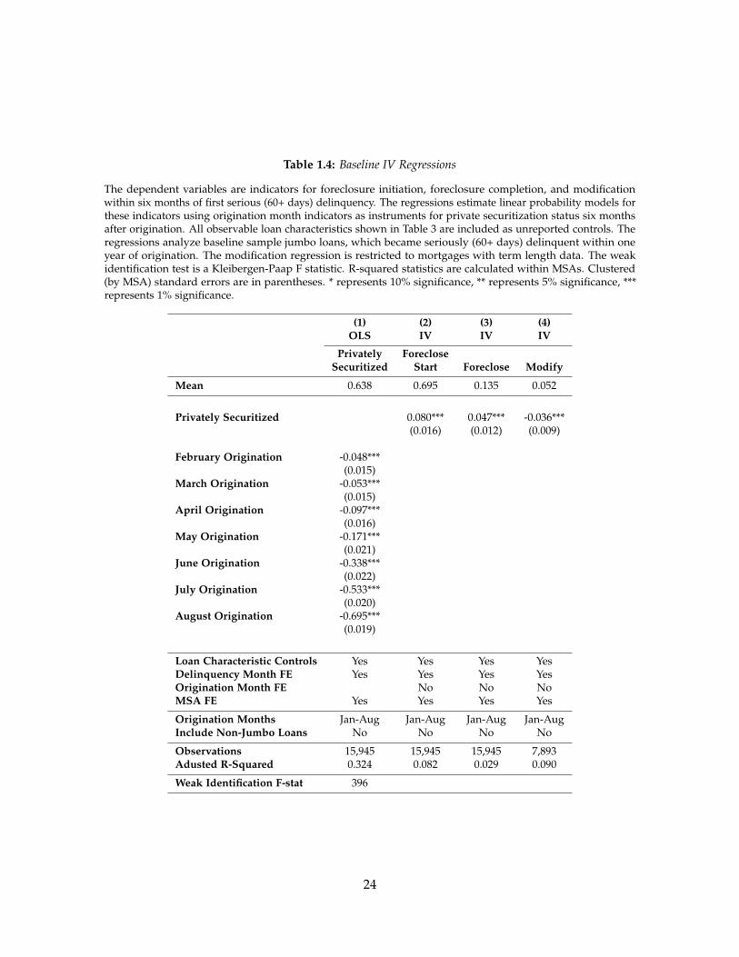
Table 1.4: Baseline IV Regressions

The dependent variables are indicators for foreclosure initiation, foreclosure completion, and modificationwithin six months of first serious (60+ days) delinquency. The regressions estimate linear probability models forthese indicators using origination month indicators as instruments for private securitization status six monthsafter origination. All observable loan characteristics shown in Table 3 are included as unreported controls. Theregressions analyze baseline sample jumbo loans, which became seriously (60+ days) delinquent within oneyear of origination. The modification regression is restricted to mortgages with term length data. The weakidentification test is a Kleibergen-Paap F statistic. R-squared statistics are calculated within MSAs. Clustered(by MSA) standard errors are in parentheses. * represents 10% significance, ** represents 5% significance, ***represents 1% significance.

(1) (2) (3) (4)OLS IV IV IV

Privately ForecloseSecuritized Start Foreclose Modify

Mean 0.638 0.695 0.135 0.052


February Origination -0.048***(0.015)

March Origination -0.053***(0.015)

April Origination -0.097***(0.016)

May Origination -0.171***(0.021)

June Origination -0.338***(0.022)

July Origination -0.533***(0.020)

August Origination -0.695***(0.019)

Loan Characteristic Controls Yes Yes Yes YesDelinquency Month FE Yes Yes Yes YesOrigination Month FE No No NoMSA FE Yes Yes Yes Yes

Origination Months Jan-Aug Jan-Aug Jan-Aug Jan-AugInclude Non-Jumbo Loans No No No No

Observations 15,945 15,945 15,945 7,893Adusted R-Squared 0.324 0.082 0.029 0.090

Weak Identification F-stat 396

24

Private securitization decreases the six-month probability of modification by 3.6 ppt. The

coefficient estimates are all statistically significant (standard errors range from 0.9 ppt

to 1.6 ppt). Moreover, they are economically large. As percentages of mean rates, the

foreclosure initiation coefficient is 12%, the foreclosure completion coefficient is 35%, and

the modification coefficient is 69%. Comparing columns (2) to (4) of Table 1.4 to Table 1.3

reveals the omitted variable bias of the OLS regressions. For foreclosure initiation and

completion, the IV securitization coefficient estimates are about twice as large as their OLS

counterparts. On the other hand, the OLS and IV estimates are similar for modification. It

appears that unobserved quality differences between securitized and portfolio loans make

securitized loans less likely to be foreclosed without having much effect on modification.

As a result OLS underestimates the causal impact of securitization on foreclosure.

1.4.2 Interpreting the Results

The IV estimates of Table 1.4 estimate the Local Average Treatment Effect (LATE) of private

securitization on foreclosure and modification. The securitization freeze instrument affected

securitization probability for loans that would have been securitized after a delay. The IV

methodology cannot estimate the impact of securitization on non-compliers, in this case

mortgages that never would have been securitized and mortgages that were securitized

quickly enough to avoid the freeze. Is LATE likely to differ from the Average Treatment

Effect (ATE) of securitization on all loans? No. First, the instrument is very strong (e.g., the

August first stage fixed effect is -69.5 ppt), suggesting that most mortgages are compliers.

Second, there is no a priori reason to think that speed of securitization is correlated with the

treatment effect. If the treatment effect does vary across loans, the loans and originators

with the smallest treatment effect are likely the most inclined to securitization (because a

smaller treatment effect makes securitization less costly). Thus, if anything LATE is likely

conservative relative to ATE.

The treatment itself is also slightly nuanced in the IV regression. Specifically, the IV

treatment is being stuck holding loans intended for securitization. If pre-planning aids

25

portfolio loan servicing or if the entities stuck holding the loans don’t typically engage in

portfolio lending, this treatment is slightly different from a planned changed in securitization

practices. To the extent that it matters, the lack of pre-planning likely decreases an owner’s

ability to differentially service portfolio loans, thereby making the IV estimates conservative.

A final issue of interpretation is how broadly to extrapolate the results. Strictly speaking,

my baseline regressions estimate the impact of private securitization on foreclosure and

modification of jumbo loans originated in 2007 that became delinquent within one year of

origination. In later regressions, I show that similar results also hold for loans that became

delinquent at other times. I focus on 2007 originations solely for identification purposes.

As far as I know, there is nothing special about 2007 origination practices so my coefficient

estimates should be valid for jumbo loans originated at other times. The estimates are

also informative about private securitization of non-jumbo loans (e.g., subprime loans).

Exact magnitudes may differ, but the same basic frictions of private securitization likely

apply there as well. My results are less informative about GSE securitization because GSE

securitization involves different contracts and leaves a single entity (the GSE) with full credit

exposure for the underlying mortgages.

1.4.3 Robustness Checks

One difference between my empirical design and that of Piskorski, Seru, and Vig (2010)

and Adelino, Gerardi, and Willen (2011b) is that I use a six month analysis window instead

of considering loans for a longer period of time after delinquency.25 The shorter window

is desirable because it ends before HAMP, but it creates the possibility that I am picking

up acceleration or deceleration in foreclosure and modification as opposed to changes to

their ultimate probability. Columns (1) to (3) of Table 1.5, Panel A address this concern by

replicating my baseline results with a twelve-month window instead of a six-month window.

The coefficient estimates are consistent with my baseline results. The foreclosure start

25Piskorski, Seru, and Vig (2010) consider all foreclosure actions up to the first quarter of 2008, which couldbe as much as three years after a loan becomes seriously delinquent. Adelino, Gerardi, and Willen (2011b) use atwelve-month analysis window.

26

Table 1.5: Robustness Checks

Regressions are the same as columns 2-4 of Table 4 except where noted. Columns 1-3 of Panel A considerforeclosure and modification within twelve months instead of six months. Columns 4-6 of Panel A analyze onlyloans originated between May and July of 2007. Columns 1-3 of Panel B control for originination-month fixedeffects using non-jumbo loans. Columns 4-6 of Panel B estimate bivariate probit models without MSA fixedeffects. R-squared statistics are calculated within MSAs. Clustered (by MSA) standard errors are in parentheses.* represents 10% significance, ** represents 5% significance, *** represents 1% significance.

A. 12-month analysis window and restricted origination-month sample

(1) (2) (3) (4) (5) (6)IV IV IV IV IV IV

Foreclose ForecloseStart Foreclose Modify Start Foreclose Modify

(12 mos.) (12 mos.) (12 mos.) (6 mos.) (6 mos.) (6 mos.)

Mean 0.807 0.369 0.085 0.669 0.109 0.061

Privately Securitized 0.081*** 0.061*** -0.066*** 0.078** 0.042* -0.080***(0.013) (0.016) (0.014) (0.035) (0.023) (0.025)

Loan Characteristics Yes Yes Yes Yes Yes YesDelinquency Month FE Yes Yes Yes Yes Yes YesOrigination Month FE No No No No No NoMSA FE Yes Yes Yes Yes Yes Yes

Origination Months Jan-Aug Jan-Aug Jan-Aug May-Jul May-Jul May-JulInclude Non-Jumbo Loans No No No No No No

Observations 15,945 15,945 7,893 6,443 6,443 3,259Adusted R-Squared 0.045 0.072 0.100 0.074 0.017 0.066

B. Non-jumbo origination month control regressions and bivariate probit models

(1) (2) (3) (4) (5) (6)Bivarite Bivarite Bivarite

IV IV IV Probit Probit Probit


(6 mos.) (6 mos.) (6 mos.) (6 mos.) (6 mos.) (6 mos.)

Mean 0.695 0.135 0.052 0.695 0.135 0.052

Privately Securitized 0.097*** 0.059*** -0.027** 0.068*** 0.041** -0.019(0.019) (0.015) (0.012) (0.016) (0.014) (0.012)

Loan Characteristics Yes Yes Yes Yes Yes YesDelinquency Month FE Yes Yes Yes Yes Yes YesOrigination Month FE Yes Yes Yes No No NoMSA FE Yes Yes Yes No No No

Origination Months Jan-Aug Jan-Aug Jan-Aug Jan-Aug Jan-Aug Jan-AugInclude Non-Jumbo Loans Yes Yes Yes No No No

Observations 77,160 77,160 35,934 15,980 15,980 7,931Adusted R-Squared 0.083 0.037 0.073

27

coefficient (8.1 ppt) is almost identical. The foreclosure completion coefficient is somewhat

larger (6.1 ppt compared to 4.7 ppt). The modification coefficient is more significantly larger

(-6.6 ppt compared to -3.6 ppt). The increases are likely due to the higher incidence of

foreclosure completion and modification within the twelve-month window. In short, my

baseline results appear to reflect permanent effects as opposed to changes in timing.

Another potential concern is that the jumbo lending environment changed between

January and August of 2007 or that the securitization freeze was anticipated, particularly

late in the sample. The best evidence against this concern is that the jumbo private

securitization rate stayed stable in the 80-85% range from January to April and then dropped

dramatically to 36% by August without a significant drop in originations until September

(see Figures 1.3 and 1.4). Loan volume would have dropped sooner if the securitization

freeze was anticipated, and other changes to jumbo lending this sudden and large are

unlikely especially after controlling for observable characteristics. Nonetheless, I address

the concern by restricting the sample and estimating origination-month fixed effects with

non-jumbo loans.

The restricted sample focuses on loans originated between May and July of 2007. The

probability of securitization dropped significantly over these three months from 77% in May

to 54% in July, and ending the sample before August reduces the concern that securitization

market changes may have been anticipated at the time of origination. Columns (4) to (6) of

Table 1.5, Panel A show regression estimates for the restricted sample. Standard errors are

larger, but the foreclosure coefficient estimates are nearly identical to my baseline results.

The modification coefficient is larger in the restricted sample (-8.0 ppt compared to -3.6 ppt),

suggesting that my baseline results are conservative.

To explicitly control for changes to the lending environment over time, I estimate

equation (1.2) using interactions between origination month indicator variables and jumbo

status as instruments for private securitization. As discussed earlier, this difference in

differences strategy controls for origination month fixed effects using non-jumbo loans while

using the interacted version of origination month to instrument for jumbo securitization.

28

Results are reported in Columns (1) to (3) of Table 1.5, Panel B. Foreclosure initiation (9.7

ppt), foreclosure completion (5.9 ppt), and modification (-2.7 ppt) coefficient estimates are

all close to their baseline values.

In Columns (4) to (6) of Table 1.5, Panel B, I report marginal effect estimates from

bivariate probit models. As discussed by Wooldridge (2002), this specification implements

instrumental variables identification while bounding outcome (foreclosure or modification)

and treatment (securitization) probabilities between 0 and 1 with probit functions. To avoid

biases associated with a large number of fixed effects, I drop the MSA fixed effects. The

marginal effects of private securitization on foreclosure initiation (6.8 ppt) and foreclosure

completion (4.1 ppt) are close to my baseline estimates. The modification marginal effect

(-1.9 ppt) is lower than my baseline estimate.

In the appendix, I consider three additional robustness tests: dropping loan characteristic

control variables, estimating equation (1.2) without the NonJumboi ∗ Seci interaction term,

and including mortgages that are transferred to non-LPS servicers. Results are consistent

with my baseline estimates.

1.4.4 Full Sample Results

So far my analysis has focused on my baseline sample of loans that became seriously

delinquent within twelve months of origination. The rationale for starting with this sample

is that it ends the analysis in February of 2009, before significant government intervention

into the mortgage market. The baseline sample time period (primarily 2007 and 2008) also

represents the heart of the financial crisis and was a time when servicers may have been

overwhelmed by a surge in delinquencies.

To assess whether my baseline results are specific to 2007 and 2008, I repeat my analysis

on the full sample of all jumbo loans that became seriously delinquent before 2012. Table 1.6

reports the results. The full sample private securitization coefficient estimates are 12.4 ppt

for foreclosure initiation, 2.8 ppt for foreclosure completion, and -5.1 ppt for modification

(25%, 49%, and 72%, respectively, as a percent of mean rates). Compared to the baseline

29

Table 1.6: Full Sample IV Regressions

Regressions are the same as in Table 4 except that the sample is expanded to include all jumbo sample loans thatbecame delinquent prior to 2012. The dependent variables are indicators for foreclosure initiation, foreclosurecompletion, and modification within six months of first serious (60+ days) delinquency. The regressionsestimate linear probability models for these indicators using origination month indicators as instruments forprivate securitization status six months after origination. All observable loan characteristics shown in Table3 are included as unreported controls. R-squared statistics are calculated within MSAs. Clustered (by MSA)standard errors are in parentheses. * represents 10% significance, ** represents 5% significance, *** represents1% significance.

(1) (2) (3)IV IV IV

ForecloseStart Foreclose Modify

Mean 0.488 0.057 0.071


Loan Characteristic Controls Yes Yes YesDelinquency Month FE Yes Yes YesOrigination Month FE No No NoMSA FE Yes Yes Yes



sample (Table 1.4) results, the foreclosure initiation coefficient is larger both in absolute

terms and as a fraction of the mean foreclosure initiation rate. The foreclosure completion

coefficient is lower in absolute terms but is higher as a fraction of the mean foreclosure

completion rate. The modification coefficient is larger on an absolute basis and about the

same size as a fraction of the mean modification rate.

To incentivize mortgage modifications and make modification practices more uniform,

the Obama administration enacted the Home Affordable Modification Program (HAMP)

in February of 2009. The program was rolled out over the course of 2009 and was fully

operational by the end of the year. Potential HAMP modifications are evaluated using

a standardized NPV test. If the NPV test indicates that modification is more beneficial

to the lender than foreclosure would be, the servicer employs a four-step waterfall to

30

reduce monthly payments to 31% of income by first capitalizing past-due balances, then

reducing interest rates to as low as 2%,26 then extending loan terms to up to 40 years from

the modification date, and then forbearing principal. Servicers receive $1000 of incentive

compensation per HAMP modification and success fees of up to $1000 per year for three

years for performing modifications. Borrowers can also earn up to $1000 in principal

forgiveness per year for five years for keeping modified mortgages current. HAMP does

not override specific contractual restrictions, but it does create safe harbors for servicers

by deeming the HAMP NPV tests to be the appropriate measure of investor welfare and

deeming the waterfall modification methodology to be standard industry practice. HAMP

is a voluntary program, but all major servicers participate, and participating servicers are

required to use HAMP modification guidelines for all qualifying mortgages, whether they

are privately securitized or held as portfolio loans.

HAMP’s efficacy is the subject of an ongoing debate.27 My methodology does not

provide a way to test whether HAMP succeeded in reducing foreclosures, but I can assess

whether it made foreclosure and modification decisions more uniform across securitized

and portfolio loans. Policy makers were particularly concerned about the perceived bias of

securitized loans towards foreclosure and away from modification. Was HAMP successful

at mitigating this bias?

To assess post-HAMP securitization biases, I repeat my empirical strategy on sub-

samples of jumbo loans split by the year in which they became delinquent. Table 1.7 reports

the results. Foreclosure initiation coefficients (Panel A) had no clear trend over time. If

anything, they were higher in 2010 and 2011 after HAMP was implemented, especially

when considered as a fraction of mean foreclosure initiation rates, which declined over time.

Foreclosure completion coefficients (Panel B) declined over time on an absolute basis but

26Interest rate reductions are permanent unless they are reduced below prevailing interest rates, whichestablish an Interest Rate Cap. If interest rates are reduced below the cap, they stay at the reduced level for fiveyears and then are gradually increased to the cap.

27For example, Agarwal, et al. (2012a) argue that HAMP increased modifications but has fallen short ofprogram goals because of mixed servicer compliance.

31

Table 1.7: IV Regressions by Delinquency Year

Regressions are the same as in Table 6 except that the sample is split by the year in which a mortgage firstbecomes seriously (60+ days) delinquent. The dependent variables are indicators for foreclosure initiation(panel A), foreclosure completion (panel B), and modification (panel C) within six months of first seriousdelinquency. The regressions estimate linear probability models for these indicators using origination-monthindicators as instruments for private securitization status six months after origination. All observable loancharacteristics shown in Table 3 are included as unreported controls. R-squared statistics are calculated withinMSAs. Clustered (by MSA) standard errors are in parentheses. * represents 10% significance, ** represents 5%significance, *** represents 1% significance.

A. Foreclosure initiation within six months

(1) (2) (3) (4) (5)IV IV IV IV IV

Deliquency Year 2007 2008 2009 2010 2011

Mean 0.766 0.573 0.460 0.318 0.396

Privately Securitized 0.079*** 0.125*** 0.119*** 0.167*** 0.085***(0.029) (0.016) (0.013) (0.018) (0.028)

Observations 7,647 27,520 32,514 15,937 9,537Adusted R-Squared 0.042 0.086 0.088 0.066 0.027

B. Foreclosure completion within six months

(1) (2) (3) (4) (5)IV IV IV IV IV

Deliquency Year 2007 2008 2009 2010 2011

Mean 0.173 0.064 0.036 0.035 0.048

Privately Securitized 0.062*** 0.038*** 0.013** 0.036*** 0.024**(0.022) (0.006) (0.006) (0.009) (0.010)


C. Modification within six months

(1) (2) (3) (4) (5)IV IV IV IV IV

Deliquency Year 2007 2008 2009 2010 2011

Mean 0.045 0.064 0.068 0.078 0.105

Privately Securitized -0.022* -0.070*** -0.042*** -0.021 -0.072**(0.013) (0.009) (0.010) (0.014) (0.033)


32

increased as a fraction of mean foreclosure rates. Modification coefficients (Panel C) had

no trend over time on an absolute basis and decreased moderately as a fraction of mean

modification rates. With the sole exception of modification in 2010, private securitization

increased foreclosure and decreased modification probability by statistically significant

and economically meaningful amounts in all years. In short, there is no evidence that

HAMP mitigated the bias of privately securitized loans toward foreclosure and away from

modification.

Direct comparisons between pre-HAMP and post-HAMP coefficients are somewhat

problematic because it is not clear exactly what the counterfactuals should be. Even aside

from HAMP policy changes, the regressions consider different time periods and the loans

analyzed have different ages. Nonetheless, the fact that the foreclosure and modification

biases persisted after HAMP suggests that HAMP had little impact on them. At the very

least we can conclude that HAMP did not fully eliminate the bias of privately securitized

loans toward foreclosure and away from modification.

1.4.5 Long Term Impact

Private securitization increases the probability of foreclosure and decreases the probability

of modification within six and twelve months of first serious delinquency. Do these effects

also show up in longer term foreclosure and modification probabilities? How large are the

long term effects? What is the total impact of private securitization on foreclosures?

To answer these questions, I estimate the impact of private securitization on foreclosure

and modification over a three-year analysis window. The analyzed sample includes all

jumbo loans that became seriously delinquent before 2010. Table 1.8 reports the results.

Private securitization increases the three-year probability of foreclosure initiation by 8.7 ppt,

increases three-year probability of foreclosure completion by 11.3 ppt, and decreases the

three year probability of modification by 5.9 ppt. As a fraction of mean rates these represent

impacts of 11% for foreclosure initiation, 31% for foreclosure completion, and -25% for

modification.

33

Table 1.8: IV Regressions with a 3-Year Analysis Window (Full Sample)

Regressions are the same as in Table 6 except that the dependent variables are now foreclosure initiation,foreclosure completion, and modification within three years instead of six months. The sample is jumbo loansthat became delinquent prior to 2010. The regressions estimate linear probability models using originationmonth indicators as instruments for private securitization status six months after origination. All observableloan characteristics shown in Table 3 are included as unreported controls. R-squared statistics are calculatedwithin MSAs. Clustered (by MSA) standard errors are in parentheses. * represents 10% significance, ** represents5% significance, *** represents 1% significance.

(1) (2) (3)IV IV IV


(3 Years) (3 Years) (3 Years)

Mean 0.789 0.369 0.235


Loan Characteristic Controls Yes Yes YesDelinquency Month FE Yes Yes YesOrigination Month FE No No NoMSA FE Yes Yes Yes



Since September of 2008, 4.4 million homes have been foreclosed, half of which were

privately securitized.28 If private securitization increased the incidence of foreclosure by 31%,

this means over 500,000 foreclosures are attributable to private securitization. Admittedly,

this is a rough estimate. It requires extrapolation from jumbo private securitization to

private securitization more generally, and it ignores the general equilibrium effects of

curtailing private securitization. That said, 500,000 could actually be a conservative estimate.

Subprime private securitization frictions may be even larger than jumbo frictions, and

curtailing securitization may have increased loan quality, further decreasing delinquencies

and foreclosures.

28Foreclosure data is from the CoreLogic National Foreclosure Report, April 2013. Piskorski, Seru, and Vig(2011) and Mayer (2009) estimate that half of foreclosure initiations were privately securitized mortgages basedon Federal Reserve reports and private market data.

34

1.4.6 Modification Details and Effectiveness

In addition to impacting the probability of modification, securitization also affects how loans

are modified. Some securitized servicing contracts place limits on principal and interest

reductions and modifications and term extensions. Further, servicers of securitized loans

may have an incentive to keep delinquent loans alive longer through principal-increasing

modifications that capitalize past due balances. Finally, servicers of securitized loans may

have less incentive to invest in thoughtful screening and negotiation to give modifications

the best chance of successfully preventing future default.

To assess the impact of securitization on modification terms, I employ my IV regression

strategy on the subset of delinquencies that are modified. For this analysis I include all

jumbo loans that became seriously delinquent before 2012 and were modified within six

months. First, I consider indicators for different types of modifications as my dependent

variables, thereby estimating the probability of a certain type of modification conditional on

there being a modification of some kind. Except for the different sample and dependent

variables, the regressions are identical to my previous IV regressions. Panel A of Table

1.9 reports the results. Securitization increases the incidence of interest modifications and

principal increases, decreases the incidence of term modifications, and has no significant

impact on the incidence of principal decreases.

I also consider how securitization affects net changes to interest rates, term lengths,

principal balances, and monthly payments. Panel B of Table 1.9 reports results for regressions

of net changes on the same variables considered in Panel A. Across all terms, privately

securitized modifications are less concessionary. Even though a higher fraction of privately

securitized modifications involve interest rate decreases, the average interest rate decrease is

39 bps lower for securitized mortgages. Similarly, term extensions and payment cuts are

smaller and principal increases are larger for privately securitized mortgages.

Finally, I compare the effectiveness of securitized and portfolio modifications by ana-

lyzing the probability of redefault (return to 60+ day delinquency) in the twelve months

following modifications that cured delinquencies. Table 1.10 reports the results. In column

35

Table 1.9: Modification Details (Full Sample)

All regressions are conditional on loans being modified. The dependent variables in Panel A are indicators forinterest rate modification, term modification, principal decrease, and principal increase. Panel A regressionsestimate linear probability models for these indicators. The dependent variables in Panel B are net changes tointerest rates, term lengths, principal balances, and monthly payments. Private securitization status six monthsafter origination is instrumented with origination-month indicators. All observable loan characteristics shownin Table 3 are included as unreported controls. The regressions analyze jumbo loans that became seriouslydelinquent before 2012 and are modified within six months of becoming seriously delinquent. The net change(Panel B) regressions exclude observations with extreme changes (rate changes over 10 ppt, term changes over20 years, principal changes over 50%, and payment changes over 75%). R-squared statistics are calculated withinMSAs. Clustered (by MSA) standard errors are in parentheses. * represents 10% significance, ** represents 5%significance, *** represents 1% significance.

A. Type of modification

(1) (2) (3) (4)IV IV IV IV

Interest Term Principal PrincipalModification Modification Decrease Increase

Mean 0.343 0.375 0.058 0.509

Private Security 0.058** -0.427*** -0.021 0.448***(0.023) (0.030) (0.020) (0.039)

Loan Characteristic Controls Yes Yes Yes YesDelinquency Month FE Yes Yes Yes YesOrigination Month FE No No No NoMSA FE Yes Yes Yes Yes



B. Net changes

(1) (2) (3) (4)IV IV IV IV

Interest Term Principal PaymentChange (ppt) Change (mos.) Change (%) Change (%)

Mean -2.792 25.733 0.259 -27.302

Privately Securitized 0.385** -68.693*** 1.573** 4.034**(0.161) (5.555) (0.717) (2.047)

Loan Characteristic Controls Yes Yes Yes YesDelinquency Month FE Yes Yes Yes YesOrigination Month FE No No No NoMSA FE Yes Yes Yes Yes



36

Table 1.10: Modification Effectiveness (Full Sample)

All regressions are conditional on a loan being cured of initial delinquency with a loan modification. Thedependent variable is an indicator for redefault, defined as a return to 60+ day delinquent status within oneyear of modification. The regressions estimate linear probability models using origination month indicatorsas instruments for private securitization status six months after origination. Indicators for modification typeare included where indicated. All observable loan characteristics shown in Table 3 are included as unreportedcontrols. The regressions analyze jumbo loans that were cured through modification before 2012 within sixmonths of becoming seriously delinquent. R-squared statistics are calculated within MSAs. Clustered (by MSA)standard errors are in parentheses. * represents 10% significance, ** represents 5% significance, *** represents1% significance.

(1) (2)IV IV

Redefault Redefault

Mean 0.302 0.302

Privately Securitized 0.076** 0.042(0.034) (0.045)

Interest Decrease -0.094***(0.027)

Term Increase -0.046(0.031)

Principal Decrease -0.096***(0.032)

Principal Increase 0.048*(0.029)

Loan Characteristic Controls Yes YesDelinquency Month FE Yes YesOrigination Month FE No NoMSA FE Yes Yes

Origination Months Jan-Aug Jan-AugInclude Non-Jumbo Loans No No

Observations 3,058 3,058Adusted R-Squared 0.199 0.210

37

(1), I estimate an IV regression of redefault on private securitization and standard controls

in the full sample of jumbo loans. Redefault is 7.6 ppt higher for privately securitized loans

(compared to a mean redefault rate of 30%). The difference is partially explained by the

types of modifications employed. Column (2) includes controls for modification type. This

decreases the private securitization coefficient to (a statistically insignificant) 4.2 ppt. Interest

and principal decreases are associated with lower redefault rates. Principal increases are

associated with higher redefault rates.29

1.5 Mechanism

The preceding section established that privately securitized loans are foreclosed more and

modified less than comparable portfolio loans. Why do servicers treat securitized loans and

portfolio loans differently?

Servicing securitized mortgages is a classic principal-agent problem. Securitized mort-

gages are owned by trusts that are explicitly passive (in part for tax reasons) and managed

by third party servicers. Servicing current mortgages is relatively straight-forward. Servicers

bill mortgagors, collect and forward payments, and maintain records. These functions can be

readily standardized and specified in servicing contracts. By contrast, servicing delinquent

loans is highly discretionary. Collection, modification, and foreclosure involve unobservable

actions and loan-specific decisions that are difficult to specify in advance.

As in other principal-agent settings, servicing practices can deviate from investor inter-

ests either because of contract rigidity or because servicer incentives differ from investor

incentives. The most obvious case of contract rigidity is explicit prohibitions of certain

practices, particularly modification. These restrictions are meant to protect investors but

may end up hurting them in some situations. Incentive differences are primarily manifested

in an incentive for servicers to underinvest in practices that could enhance a mortgage’s

value but would be costly to the servicer. Servicers may also have an incentive to not deviate

29These results are qualitatively similar to Agarwal, et al.’s (2011) OLS estimate that redefault is 3.5% higherfor securitized modifications relative to portfolio modifications.

38

from default practices. For example, if foreclosure is the default practice for delinquent

loans, servicers may perceive that alternatives invite investor scrutiny and liability risk.

In some principal-agent settings, deviations from the principal’s preferred actions can be

corrected with ex-post renegotiation. This is all but impossible for MBS because dispersed

investors lack the ability and incentive to monitor servicers.30 Amending servicing contracts

is also a difficult process, requiring super-majorities of certificateholders.

Previous discussions have focused mainly on securitization impeding mortgage modifi-

cation, often with an emphasis on contractual modification restrictions, and this spilling over

into increased foreclosure rates. This is an incomplete view of how securitization impacts

delinquent mortgage servicing. Binding contractual restrictions on modifications are rare,

and spillovers from decreased modifications are only part of the bias of securitized loans

towards foreclosure. We have already seen one piece of evidence to this effect. Securitiza-

tion has a larger impact on foreclosure (8.0 ppt for foreclosure initiation and 4.7 ppt for

foreclosure completion) than on modification (-3.6 ppt). If the foreclosure bias was solely a

spillover from modification frictions, it should be smaller than the modification bias.

To better understand how securitization affects mortgage servicing, I examine the

contractual terms of actual servicing agreements and link these terms to loan-level panel

data on modifications and foreclosures. I find that reimbursement policies universally

incentivize foreclosure over modification and other effort-intensive loss mitigation practices.

In contrast, binding modification restrictions are rare and have only moderate impact on

modification rates.

1.5.1 Servicing Practices

Before focussing on frictions associated with servicing securitized loans, it is important to

understand the options available to servicers when dealing with delinquent loans. Foreclo-

sure and modification are not binary responses to delinquency. Servicers also have a wide

30MBS trusts have trustees that theoretically represent the interests of certificateholders, but the actual powerand responsibility of trustees are limited, and servicers can only be removed in exceptional situations. Moreover,a trustee is just another agent for the underlying investors with its own conflicts of interest.

39

range of notification, collection, relief, and loss mitigation options. Securitization has the

potential to bias whether and how all of these options are used.

Fannie Mae’s 2006 Servicing Guide offers a window into the breadth of delinquency

management practices available to servicers. Notification options include late payment

notices, payment reminder notices, reminder phone calls, letters (preferably individually-

written as opposed to form letters), and face-to-face interviews. If communication alone

does not suffice, Fannie Mae has procedures for debt collection by attorneys, acceptance

or rejection of partial payments, referral to counseling agencies, and direct delinquency

counseling. In parallel with these efforts, servicers are to communicate with junior lien-

holders. If a temporary hardship is identified, servicers may offer special relief in the

form of a 30-day grace period, longer forbearance agreement, or repayment plan to pay

past-due balances over time on top of regular monthly payments. With Fannie Mae approval,

servicers can also negotiate more formal “Loss Mitigation Alternatives,” including loan

modifications, short sales, deeds-in-lieu of foreclosure, assumptions of mortgages by new

homebuyers, and assignment of mortgages to mortgage insurers.

Choosing among these options requires significant servicer discretion. Optimal practices

depend on loan-specific soft information that is difficult to document and essentially

impossible to contract on ex-ante. Moreover, most delinquency management practices

involve personal interaction with borrowers, which makes them costly and dependent on

unobservable effort. Modification is particularly challenging because it requires servicers to

negotiate new mortgage terms, which have the potential to harm investors.

Levitin and Twomey (2011) contrast foreclosure with other delinquency management

tools. Foreclosure is unique in that once undertaken it involves little discretion and can be

largely outsourced and automated. For example, Levitin and Twomey describe a widely

used software platform that automatically refers mortgages to approved local attorneys once

certain delinquency benchmarks (e.g., 60 days past due) are reached. The software uploads

required documents for the attorneys and generates specific instructions and timelines

without any human contact.

40

All servicers face a decision as to how much they should automate delinquent loan

servicing. At one extreme, decisions can be highly formulaic and push most delinquent

borrowers into foreclosure. At the other extreme, servicing can be hands-on with significant

personal interaction and solutions tailored to specific borrower circumstances. The basic

trade-off is servicing cost versus higher recovery rates. Levitin and Twomey (2011), argue

that faced with this tradeoff most servicers chose the scale efficiencies of heavy automation.

They further argue that the tradeoff between automation and hands-on discretion changed

as delinquency rates climbed in 2007 and 2008 but that servicers were ill-equipped to quickly

ramp up non-foreclosure delinquency management capabilities.

Securitization introduces three additional elements into this tradeoff. First, because it

involves less discretion, soft information, and unobservable effort, automation mitigates

principal-agent conflicts. Second, because it is cheaper, securitized servicers will naturally

choose automation. Overcoming the bias towards automation requires costly interventions

such as incentive payments or contractual restrictions of servicer actions. These elements

both make automation more ex-ante efficient for securitized servicing relative to portfolio

servicing. The final element is that servicing agreements are locked in when a deal closes

and are difficult, if not impossible, to alter in response to changing market conditions. Thus,

automation is sticky for securitized servicing even if market conditions change to favor

more hands-on discretion.

1.5.2 Servicing Agreements

Securitized mortgage servicing is governed by servicing agreements, which are incorporated

into more general pooling and servicing agreements (PSAs). To understand how these

agreements operate, I analyze the terms of actual PSAs. My sample consists of all prime

MBS deals between January and August of 2007 that exceeded $1B. 37 deals meet this

criteria, which collectively represent $70B, 48% of total prime MBS issuance during this

41

period.31 For deals that involve multiple servicing agreements, I describe the agreement

that is relevant to the most loans. The sample covers nine deal sponsors and seven servicers.

The PSAs give servicers broad authority for managing loans coupled with responsibility

to follow accepted industry practices. Servicers bear most costs of servicing the loans and

are compensated with a servicing fee, which is typically around 25 bps annualized for

prime mortgages. Servicing fees are payable from loan proceeds and (in case of default)

from the trust more generally so they function as a senior interest only strip for the life of

a loan. Servicers also retain late fees and other ancillary fee income. Servicers generally

have discretion to pursue modifications and other loss mitigation alternatives, but they have

little direct incentive to do so because these tools require unreimbursable expenses and may

involve waiving fee income. By contrast, foreclosure expenses are fully reimbursed. As long

as they comply with accepted industry practices, servicers have an incentive to shade their

delinquency management practices away from modification and loss mitigation and toward

foreclosure. This incentive is compounded by the fact that foreclosure is universally specified

as a default practice for delinquent loans, which may make it less risky for servicers from

an investor liability point of view. Some PSAs contractually prohibit certain modifications,

but these restrictions are relatively uncommon.

Table 1.11 summarizes the incidence of specific PSA terms. Sample PSAs universally

require servicers to follow accepted servicing practices, generally defined as the practices of

other responsible mortgage lenders. One source of these practices is Fannie Mae servicing

guidelines, which are explicitly incorporated into 38% of PSAs. 68% of PSAs also require

that loans be serviced equivalently to portfolio loans, and in one case the PSA explicitly

requires that servicing be in the best interest of certificateholders. In other PSAs this is

implicit in general and sometimes an explicit standard for specific servicing decisions.

The PSAs also universally establish a default responsibility to foreclose on sufficiently

31Data on MBS issuance volumes comes from Inside Mortgage Finance. Classifications of individual MBSdeals come from Inside Mortgage Finance and review of prospectuses and rating agency reports for individualdeals. In addition to the 37 deals in my sample, Inside Mortgage Finance identifies another 10 deals as primethat are described as Alt-A by the ratings agencies.

42

Table 1.11: Summary of PSA Terms

The sample consists of all prime non-agency MBS deals in excess of $1B closed between January and August of2007. 37 MBS deals with a total of value of $70B meet this criteria. These deals represent 48% of total January -August 2007 prime non-agency MBS volume. For deals with multiple pooling and servicing agreements (PSAs)(e.g., deals involving multiple originators or servicers), the sample includes the agreements relevant to the mostloans. The sample includes nine sponsors and seven servicers.

Number of Percent ofPSAs PSAs

Representations and Warranties:Early payment default warranty 0 0%Loan schedule is accurate 37 100%Loans are current 31 84%Loans had only limited past delinquency 22 59%

Servicing:General servicing responsibilities:

Accepted industry practices 37 100%Equivalent to portfolio loans 25 68%Best interest of certificateholders 1 3%Fannie Mae Servicing Guide 14 38%

Obligation to foreclose 37 100%Foreclosure reimbursement 37 100%Obligation to modify 0 0%

Obligation to consider modification 7 19%Modification reimbursement:

From trust 0 0%From mortgagor 8 22%

Payment advances:Must advance delinquent monthly payments 37 100%If principal or interest deferred, must advance difference 22 59%

Modification restrictions:Must be in default or default is forseeable 23 62%Must expect modification value to exceed foreclosure proceeds 8 22%May not permanently decrease principal or interest rate 8 22%May not extend term beyond term of certificates 1 3%May not extend term beyond maturity of last-maturing loan 4 11%

Ammendment:Without consent:

Cure/correct terms 37 100%Alter without adversely affecting certificateholders 12 32%

Required consent for other changes:Overall majority consent 37 100%Overall supermajority (over 66%) consent 10 27%Majority or supermajority consent in all affected classes 26 70%

Prohibition on decreasing or delaying payments without universal consent 37 100%

43

delinquent loans and provide reimbursement for foreclosure expenses. PSAs allow foreclo-

sure to be postponed or avoided altogether if it is not in the best interest of certificateholders

(for example if modification is more valuable or if hazardous materials make foreclosure

more expensive than the property’s value), but these are always exceptions to the general

rule of foreclosure.

By contrast, modification and other loss mitigation practices are never explicitly required

and are not reimbursed through regular loan payments or by the trust. Instead, servicers

“may” pursue these alternatives and modify loans under certain conditions. The closest the

PSAs come to requiring modification is a term in seven deals that requires the servicer to

“consider” alternatives to foreclosure. In lieu of reimbursement from the trust, servicers

are allowed to charge borrowers a modification fee. This is explicit in 22% of PSAs and

implicit in the other PSAs by virtue of Fannie Mae’s 2006 servicing guide allowing servicers

to charge borrowers a $500 modification fee and some modification-related expenses. 59% of

PSAs also disincentivize modification by requiring servicers to advance deferred or forgiven

principal and interest payments for any modification that alters mortgage payments. These

advances will eventually be reimbursed out of the loan’s future proceeds or from the trust

more generally, but in the mean time they constitute interest-free loans from the servicer to

the trust.32

Of all the terms summarized in Table 1.11, modification restrictions vary the most and

are of most interest. Some of these terms appear to be innocuous. 62% of PSAs explicitly

prohibit principal, interest, or term modifications unless a mortgage is in default or default

is foreseeable. This restriction is unlikely to bind (it certainly does not bind for the seriously

delinquent loans I analyze) and is probably implicit in accepted servicing practices even

where it is not explicitly included. 22% of PSAs require the expected value of modified

loans to exceed the expected value of foreclosure proceeds. This is also unlikely to bind and

is implied by accepted industry practices.

32Servicers similarly advance scheduled principal and interest payments while a loan is in default until theadvances are deemed uncollectable.

44

Binding modification restrictions come in the form of limitations on principal forgive-

ness, interest reductions, and term extensions. 22% of PSAs prohibit modifications that

decrease principal balances or permanently decrease interest rates. 14% of PSAs prohibit

modifications that increase loan maturity beyond the maturity of other loans in the trust or

the maturity of the trusts’ certificates. Because loans in a deal almost always have similar

maturities (typically 30 years), this effectively prohibits term extensions. Importantly, these

restrictions are uncommon compared to the universal incentive differences described above,

and they still permit many kinds of modifications. For example, temporary interest rate

reductions and principal forbearance are permitted under all PSAs.

Finally, amendment is difficult under all of the PSAs. General amendments require at

least a majority approval of certificateholders, and in all but one PSA they require either a

supermajority of certificateholders or a majority vote within each class of affected certifi-

cateholders.33 Moreover, all PSAs expressly outlaw any amendment that would decrease

or delay payments without the universal consent of all certificateholders. Any amendment

inducing modification or other loss mitigation activity over foreclosure would presumably

trigger this prohibition. If a PSA is substantively modified, this would necessitate an 8-K

filing with the SEC. I observed no such filing for any of the 37 deals I investigated.

This is the largest survey of PSA terms that I am aware of and the only one that focuses

on prime MBS. It also describes a wider range of PSA terms than any previous study.

Three other studies survey subprime PSAs with consistent results. Hunt (2009) surveyed 20

subprime deals in 2006 and found that 67% limit modifications to loans in default or where

default is foreseeable or imminent and 10% prohibit modifications altogether. Credit Suisse

(2007) surveyed 31 deals between 2004 and 2007 and found that nearly all PSAs permit

modification of loans in default or where default is reasonably foreseeable and 60% had no

other modification restrictions. A Bear Stearns study described by Bajaj (2007) and Hunt

(2009) surveyed approximately 20 deals and found that 10% of deals prohibit modifications

33Amendments to cure or correct ambiguities and conflicts are allowed without shareholder consent,and some PSAs (32%) allow more general amendments without consent if they don’t adversely impactcertificateholders.

45

and another 40% of deals require ratings agency approval if more than 5% of a loan pool is

changed.

1.5.3 PSA Term Regressions

To assess how modification restrictions affect servicer behavior, I link PSAs to individual

loans in Core Logic panel data.34 For comparability to my earlier analysis, I limit the

dataset to jumbo loans and impose the restrictions described in Section 3.35 As described in

Table 1.12, the linked dataset includes 85,000 loans with an aggregate origination value of

$60B. The loans are similar to the jumbo loans analyzed in Section 4 but are slightly larger

($708K on average compared to $691K) and have slightly higher FICOs (742 compared to

733) and lower LTVs (0.71 compared to 0.73). The linked sample also defaults less than

the earlier sample (1% became seriously days delinquent within 1 year and 21% became

seriously days delinquent within five years compared to 6% and 36%). These differences

likely stem from the linked sample being entirely from prime MBS whereas my earlier

sample included all jumbo mortgages with FICOs above 620. My analysis focuses on 18,000

loans that became seriously delinquent between 2007 and 2011. Foreclosure initiation (51.7%

within six months), foreclosure completion (6.7% within six months) and modification (6.3%

within six months) rates are similar to the previous full jumbo sample. Foreclosure and

modification are defined and identified as before with one significant difference. I cannot

identify term extensions in the Core Logic data. Thus, term modifications are missing from

the PSA-linked data.

Having linked PSAs to individual delinquencies, I regress foreclosure and modification

probability on indicators for PSA terms. Specifically, I regress foreclosure initiation, fore-

closure completion, and modification within six months of first serious delinquency on

34Core Logic mortgage data is similar to the LPS data used for my previous analysis but is limited toprivately securitized mortgages. Unlike LPS, Core Logic contains identifiers for servicers, originators, and deals,which allows me to link loans to PSAs.

35The only changes are that I no longer require loans to enter the dataset within four months of originationand I do not require loans to be originated in 2007. Survivor bias is not an issue in the Core Logic data becauseall loans enter the dataset when a deal closes.

46

Table 1.12: PSA-Linked Loan Sample

Data comes from Core Logic loan data linked to my sample of PSAs from prime non-agency MBS deals closedbetween January and August of 2007. The sample consists of jumbo (over $417K) first-lien conventional loansthat have orgination FICO scores between 620 and 850, have origination loan-to-value ratios of less than 1.5,have terms of 15, 20, or 30 years, and are located in U.S. MSAs outside of Alaska and Hawaii. The delinquentloan sample includes loans that became seriously (60+ days) delinquent between 2007 and 2011. Delinquency is60+ day delinquency. Foreclosure initiation is the referral of a mortgage to an attorney to initiate foreclosureproceedings. Foreclosure completion is identified by post-sale foreclosure or REO status. Modifications areidentified based on observed changes to loan terms.

DelinquentAll Loans Loans

Number 85,036 18,049Size (mean) $707,542 $671,927FICO (mean) 742 722LTV (mean) 0.71 0.75

OwnershipPrivate Security 100% 100%

DelinquencyWithin 1 year 1.1%Within 5 years 20.9%

Foreclosure InitiationWithin 6 months 51.7%Within 1 year 60.6%

Foreclosure CompletionWithin 6 months 6.7%Within 1 year 20.6%

ModificationWithin 6 months 6.3%interest decrease 5.4%term extensionprincipal decrease 0.0%principal increase 2.5%

Within 1 year 13.3%

indicators for prohibitions of (1) permanent principal and interest reductions and (2) term

extensions beyond the term of the MBS certificates or other mortgages. As discussed earlier,

these terms vary across PSAs. To the extent that they bind, we should expect them to reduce

modifications and potentially increase foreclosures. The regressions are OLS and include the

same control variables as previous regressions plus servicer fixed effects. The servicer fixed

effects are important because PSA terms vary across servicers and previous studies (e.g.,

Agarwal, et al. (2011) and Agarwal, et al. (2012a)) have demonstrated that servicers employ

different modification and foreclosure practices. One caveat is that within-servicer term

47

Table 1.13: PSA Term Regressions

The dependent variables are indicators for foreclosure initiation, foreclosure completion, and modification withinsix months of first serious (60+ days) delinquency. All regressions are OLS. The reported independent variablesare indicators for the presence of servicing contract terms. All observable loan characteristics shown in Table 3are included as unreported controls. The regressions also control for MSA, origination month, delinquencymonth, and servicer fixed effects. The regressions analyze sample jumbo loans that became seriously (60+days) delinquent between 2007 and 2011. R-squared statistics are calculated within MSAs. Clustered (by MSA)standard errors are in parentheses. * represents 10% significance, ** represents 5% significance, *** represents1% significance.

(1) (2) (3)OLS OLS OLS


Mean 0.517 0.067 0.063

Permanent Principal and Interest 0.137*** 0.075*** 0.001Reductions Prohibited (0.025) (0.013) (0.011)

Term Extensions Limited 0.110*** 0.039*** -0.020*(0.028) (0.013) (0.010)

Loan Characteristic Controls Yes Yes YesServicer FE Yes Yes YesDelinquency Month FE Yes Yes YesOrigination Month FE Yes Yes YesMSA FE Yes Yes Yes


variation is limited to two servicers. Servicer A has prohibitions of permanent principal and

interest reductions in the seven deals it sponsors but not in the three deals it services for

other sponsors. Servicer B has prohibitions on term extensions in the four deals it sponsors

but not in the three deals it services for other sponsors.

Table 1.13 reports the results. Prohibitions on permanent principal and interest reduc-

tions are associated with increased foreclosure (13.7 ppt for foreclosure initiation and 7.5 ppt

for foreclosure completion) and no change in modification. Prohibitions on term extensions

are associated with increased foreclosure (11.0 ppt for foreclosure initiation and 3.9 ppt for

foreclosure completion) and slightly decreased modification (-2.0 ppt, significant at the 10%

level). Because I am unable to identify modifications that solely extend mortgage terms,

this likely underestimates the full impact of term extension prohibitions on modifications.

48

These results are directionally what we should expect. Modification restrictions decrease

modifications and increase foreclosures. However the magnitudes, particularly for mod-

ification, are too small to explain the overall bias of securitized loans toward foreclosure

and away from modification. For example, the -2.0 ppt modification bias applied to the

approximately 14% of securitized loans with this term only explains -0.3 ppt of the -3.6

ppt baseline modification bias for securitized loans. Similarly, the foreclosure coefficient

estimates, combined with the incidence of these terms explain 56% of the foreclosure start

bias and 46% of the foreclosure completion bias.

1.6 Conclusion

This paper’s contribution is threefold. First, I propose a novel instrument for jumbo

securitization and provide the first well-identified assessment of securitization’s impact on

foreclosure and modification rates. Private securitization increases foreclosure probability

(by 8.0 ppt for foreclosure initiation and 4.7 ppt for foreclosure completion) and decreases

modification probability (by 3.6 ppt). Second, I estimate the effect of securitization on

foreclosure and modification over time, including periods before and after government

intervention. Securitization increased foreclosure probability and decreased modification

probability throughout 2007 to 2011, even after implementation of the Home Affordable

Modification Program (HAMP) in 2009. Third, I identify the mechanisms through which

securitization effects foreclosure and modification, highlighting that incentive differences

are more important than contractual prohibitions and that the foreclosure bias is more than

just a spillover from modification frictions.

The bias of securitized loans towards foreclosure and away from modification helps to

explain why foreclosure is so prevalent. Securitization increases the incidence of foreclosure

completion within three years by 31%. Extrapolated to all privately securitized mortgages,

this adds up to over 500,000 of the 4.4 million foreclosures experienced since the start of

the financial crisis. Securitization does not explain all foreclosures, but many foreclosures

would have been prevented if mortgages had been held directly on bank balance sheets

49

instead of being securitized.

The differential treatment of securitized and portfolio loans serves as an example of

how ownership structure can affect how assets are managed. Despite contracts designed

to protect MBS investors from differential servicing treatment, securitized loans were

systematically foreclosed more and modified less. This is an important factor in the

debate about the welfare implications of securitized lending both in the mortgage market

and elsewhere. Previously, most assessments of mortgage securitization have focused on

origination, comparing the benefit of increased funding availability with the cost of lower-

quality underwriting. Sub-optimal servicing is another channel through which securitization

can be harmful and should be considered for both regulatory reforms and improvements to

private contracts.

Finally, a word about welfare. In a first-best world where all loans are optimally managed,

a loan’s ownership status should not affect foreclosure and modification decisions. Thus,

my results reject the hypothesis that mortgage servicing is efficient. However, this does not

mean that eliminating securitization (or correcting its biases) would make servicing perfectly

efficient. Portfolio lending is also subject to principal-agent problems, and externalities

(particularly for foreclosure) could drive a wedge between private and social welfare.

Properly interpreted, my results show the effect of adding a layer of principal-agent conflict

through securitization and highlight a mechanism that has increased foreclosure rates. This

understanding is critical for achieving the policy goal of reducing foreclosures, but it does

not pin down what the policy goal should be. The private and social costs and benefits of

foreclosure and modification remain important topics for future research to address the

broader welfare question.

50

Chapter 2

Disagreement and Liquidity

2.1 Introduction

Extensive trading of equities and other informationally sensitive securities is a puzzle.

Standard asset pricing models have no role for trading, and models that consider trading

typically predict that asymmetric information decreases trading and destroys liquidity,

defined as the ability to trade an asset without significantly changing its price. Given the

large potential for asymmetric information in stocks, corporate bonds, and stock options, it

is counterintuitive that these securities are heavily traded in liquid markets. Holmstrom

(2008) highlights this puzzle by comparing money (liquidity) markets to stock markets:

"Markets for liquidity are very different than stock markets. In the stock market, uncertainty

and adverse selection fears are present all the time, but this does not prevent the markets

from functioning.... Differences in beliefs often alleviate adverse selection. Stock markets

thrive on differences in beliefs. Markets for liquidity are killed by them."

Since Akerlof (1970), economists have recognized that asymmetric information has the

potential to destroy trade. To overcome asymmetric information, at least some trade must

be motivated by something other than rationally processed information, otherwise liquidity

will dry up, markets will freeze, and the no-trade prediction of Milgrom and Stokey (1982)

will prevail. Starting with the noisy rational expectations models of Grossman and Stiglitz

51

(1980), Hellwig (1980), and Diamond and Verrecchia (1981) and including virtually all

research on liquidity and market microstructure (most notably Kyle, 1985), this extra trading

has been modeled as exogenous noise.

Traditional asymmetric information models make two basic predictions: (1) Significant

noise trading is necessary to generate trading and liquidity; and (2) asymmetric information

decreases trading and liquidity. Hong and Stein (2007) address the first prediction, noting

that trading volume in traditional models is approximately pinned down by noise (non-

informational) trading volume. For example, in Kyle’s (1985) model exogenous noise trading

represents half of total order flow variance. In my moderate variance calibration of Diamond

and Verreccia’s (1981) model, liquidity trading is 95% of total trading volume. The New York

Stock Exchange has daily volumes in excess of $30B. Liquidity trading of that magnitude

seems implausible. One way out of this problem is to interpret noise trading more generally

and claim that the vast majority of trading is uninformed noise from irrational traders.

While theoretically possible, this is not particularly satisfying. If most trading is exogenously

assumed, we aren’t really left with a model of trading. Moreover, traditional models assume

that noise trading is not just exogenous but also orthogonal to information. This is a

critical assumption, and it is likely invalid if noise trading is driven by disagreement among

market participants. For example, if disagreement comes from overconfidence in private

information, the same trade is at once informative and noise, making noise trading perfectly

correlated with information.

Prediction (2) presents even more fundamental problems. In contrast to traditional

intuition, my empirical work shows that asymmetric information actually increases trading.

I study asymmetric information, turnover, and liquidity of stocks, corporate bonds, and

stock options.1 My analysis establishes three stylized facts: (1) Trade and liquidity are

positively correlated; (2) asymmetric information increases trade and decreases liquidity;

1I proxy for asymmetric information with analyst earnings forecast dispersion and also study periodsaround earnings announcements, which likely have elevated asymmetric information. For illiquidity, I useseveral measures of bid-ask spreads as well as Amihud’s (2002) illiq = |Return|

$Volume measure.

52

and (3) high past returns increase trade and liquidity.2 Fact (1) supports the notion that

trade and liquidity reinforce one another. Fact (2) contradicts the prediction of traditional

models that asymmetric information destroys trading. Fact (3) shows that traditional models

leave out something related to past returns.

To resolve the failures of traditional models, I propose that trading is primarily driven

by disagreement. I.e., people trade because they have different beliefs about an asset’s

value. Counterparties essentially make zero-sum bets about asset values, and they do so

fully aware that other parties disagree with them. Disagreement trading has become an

increasingly popular explanation of trading volumes (Hong and Stein, 2007, summarize

this view), but there is little existing research on the relationship between disagreement

and liquidity and virtually none on how disagreement changes asymmetric information’s

impact on trading and liquidity.

In my model of disagreement trading, belief differences stem from overconfident in-

terpretation of private information. The overconfidence bias creates trade and liquidity

even when prices fully reveal the beliefs of other agents. Moreover, because disagreement

stems from private signals, trading and liquidity can increase with asymmetric information.

Formally, I model disagreement trading among ex ante homogenous agents who simultane-

ously serve as informed traders, noise traders, and market makers. Agents are risk averse,

receive endowments of a risky asset, observe private signals about the asset’s value, and

trade the asset with one another in an anonymous public market in which market price

is visible to all agents. Agents are fully rational except for an overconfidence bias, which

causes them to overestimate the precision of their own signals. I consider two versions of

the model, a baseline model in which asset endowments are constant and a general model

in which asset endowments are stochastic. The baseline model is an adaptation of Grossman

2In equity markets, these facts have been partially shown or hinted at before. In particular, Sadka andScherbina (2007) show that analyst forecast dispersion (one proxy for asymmetric information) decreasesliquidity; Frazzini and Lamont (2007) show that turnover is elevated around earnings announcements (anotherproxy for asymmetric information); and Statman, Thorley, and Vorkink (2006) show that trading increasesfollowing high returns. I extend these findings to corporate bonds and stock options and show for the first timethat analyst dispersion increases trading, earnings announcements decrease liquidity, and past returns increaseliquidity.

53

(1976) with overconfidence. The general model is an adaptation of Diamond and Verrecchia

(1981) with overconfidence.

The baseline model describes an environment in which trading is entirely driven by

disagreement. Because supply is certain and there is no non-informational motive for

trade, prices fully reveal aggregate information (as in Grossman, 1976). Nonetheless,

overconfidence induces agents to disagree and trade, thereby generating liquidity (in

contrast to Grossman, 1976). The model’s main predictions are: (1) Overconfidence increases

trading and liquidity; (2) Private information increases trading and liquidity; and (3) Public

uncertainty decreases liquidity without affecting trading volume.

The prediction that private information increases trade and liquidity conflicts with

traditional intuition. To understand this contrast, I consider a general model that adds non-

informational liquidity trading, modeled through stochastic endowments, to the baseline

model. When some trading is uninformed, increasing private information can destroy

liquidity by increasing the share of informed trade relative to uninformed trade. Private

information increases a trade’s price impact by increasing the probability that the trade

is informed. In the baseline model, all trade is informed so this channel is inoperative.

More generally, the probability that a trade is informed is insensitive to the level of private

information whenever uninformed trade is very large or very small relative to informed

trade. In these settings, traditional intuition fails, and private information increases liquidity

as in the baseline model.

My model explains trade and liquidity in the face of asymmetric information and

conforms to the stylized facts described above. It also generates the additional testable

prediction that stocks with the highest turnover response to asymmetric information should

have the smallest illiquidity response to asymmetric information.3 I test this prediction and

3Asymmetric information consists of both private information and public uncertainty. In the baselinemodel private information increases trading, whereas public uncertainty has no impact on it. Thus, asymmetricinformation changes with a larger trading impact are more likely to be driven by changes to private information.Private information enhances liquidity, whereas public uncertainty reduces it. Thus, asymmetric informationshould have the least negative impact on liquidity (and may even enhance it) when it has the most impact ontrading.

54

find that it is true in the data.

In the next section, I review related literature. Section 3 presents empirical analysis

supporting the stylized facts introduced above. Section 4 introduces, solves, and derives

comparative statics for the baseline model. Section 5 presents the general model, includ-

ing comparative statics and numerical examples of how overconfidence and asymmetric

information affect trading and liquidity. Derivations and proofs for the general model are

in an appendix. Section 6 discusses and tests the model’s empirical predictions. Section 7

concludes.

2.2 Literature Review

2.2.1 Disagreement

Disagreement models posit that a combination of private information (or private interpre-

tation of public information) and behavioral biases causes otherwise rational investors to

disagree about asset values. Disagreement models are motivated by two failings of standard

asset pricing models with homogenous beliefs. First, standard models (at least in their

simplest forms) are at odds with well-established asset pricing anomalies like momentum

(Jegadeesh and Titman, 1993), post-earnings drift (Bernard and Thomas, 1989), and long-

term return reversion (Fama and French, 1992; Lakonishok, Shleifer, and Vishny, 1994).

Second, standard models have no role for trading and thus cannot explain the high turnover

observed in many financial markets. Disagreement is an intuitively appealing rationale for

trade and, depending on what drives the disagreement, also has the potential to explain

pricing anomalies.

Hong and Stein (2007) provide a nice summary and taxonomy of disagreement models.

The first ingredient for these models is some manner of private information. One possi-

bility is that private information comes from gradual information flow as in the gradual

dissemination of information to newswatchers over time in Hong and Stein (1999). Another

possibility is that investors have limited attention and thus process only a subset of available

55

information, possibly for entirely rational reasons related to the cost of attention (e.g., Peng

and Xiong, 2006). A final possibility is that investors see the same information but interpret

it differently, possibly due to heterogeneous priors (e.g., Harris and Raviv, 1993; Kandel and

Pearson, 1995). Regardless of its source, the end result is equivalent to investors having

access private information.

The second ingredient for disagreement models is a behavioral bias in information

processing. Private information alone does not generate disagreement in standard models.

Instead, market prices aggregate and fully reveal information (Grossman, 1976), which

causes investors to agree about asset values and eliminates motives for trade (Milgrom and

Stokey, 1982). Introducing random asset supply or exogenous liquidity trading (e.g., Hellwig,

1980; Grossman and Stliglitz, 1980; Diamond and Verrecchia, 1981; Kyle, 1985) mitigates

information revelation and creates some disagreement, but trading is still largely pinned

down by assumptions about exogenous trading. For example, in Kyle’s (1985) model exoge-

nous noise trading represents half of total order flow variance. In my moderate variance

calibration of Diamond and Verreccia’s (1981) model liquidity trading is 95% of total trading

volume. To yield more significant disagreement trading, investors must value their own

information more highly than information extracted from market prices. Overconfidence

is a convenient modeling device for achieving this result and is supported by substantial

psychological evidence (see Odean, 1998; Daniel, Hirshleifer, and Subrahmanyam, 1998; and

DeBondt and Thaler, 1995, for good discussions of overconfidence). Overconfidence can be

modeled in different ways The typical approach is to assume that investors overestimate the

precision of their own signals relative to the signals of other investors.

Dynamic models of overconfidence posit that investors learn to be overconfident based

on past experience. In particular, investors are subject to a self-attribution bias that causes

them to overestimate how much their own skill was responsible for past successes. As

a result, overconfidence is highest following positive returns. Daniel, Hirshleifer, and

Subrahmanyam (1998) and Gervais and Odean (2001) model this phenomenon. Because

investors hold the market in aggregate, self-attribution bias predicts that overconfidence

56

should be high following high market returns. Stock-level overconfidence should be high

following high individual stock returns because owners of the stock just experienced high

returns. Statman, Thorley, and Vorkink (2006) show that turnover is higher than normal

following high market returns and high individual stock returns, consistent with high

returns increasing overconfidence, which in turn increases trading intensity.

Casual intuition suggests that disagreement trading should enhance liquidity. However,

liquidity has not been a major focus of the disagreement literature and is not explicitly

discussed in most disagreement papers. Exceptions include Odean (1998), Kyle, Obizhaeva,

and Wang (2013), and Baker and Stein (2004). Odean (1998) adds overconfidence to the

Kyle (1985) model of liquidity. When the informed insider receives a noisy signal and

overestimates the precision of that signal, the insider’s overconfidence increases liquidity.

Specifically, the market maker’s price function becomes less sensitive to order flow as the

insider becomes more overconfident. Though they don’t explicitly focus on liquidity, the

duopoly model of Kyle and Wang (1997) produces a similar result with two overconfident

insiders. Kyle, Obizhaeva, and Wang (2013) show that overconfidence mitigates price impact

and generates disagreement trading.4 Baker and Stein (2004) also model overconfidence

as increasing liquidity. However, this relationship is an ad hoc assumption based on the

logic that the same behavioral biases that cause investors to overestimate the precision of

their own signals will also cause them to underestimate the informational content of market

prices. None of these papers address how overconfident disagreement changes the impact

of asymmetric information on trading and liquidity.

4Kyle, Obizhaeva, and Wang’s (2013) model is the closest to my own. The main main difference betweentheir single period model and my baseline model is that investors in the Kyle, Obizhaeva, and Wang modelhave market power wherease all agents in my model are price takers. Despite the modeling similarities,Kyle, Obizhaeva, and Wang address different questions than I do. Their focus is on how market powerand overconfidence combine to give large investors an incentive to smooth trading whereas I analyze howoverconfident disagreement changes the impact of asymmetric information on trading and liquidity.

57

2.2.2 Liquidity

The market microstructure literature aims to understand what causes illiquidity in financial

markets. The backdrop is that in Walrasian equilibrium beliefs are independent from prices

and market prices perfectly reflect the demands of all agents. In real financial markets

investors learn from market prices, and prices can deviate from fundamental values creating

costs to trading. Trading costs (illiquidity) come from two main sources. First, not all

agents are active in markets at the same time. Thus, transactions must be facilitated by

market makers. These market makers must cover whatever costs they incur by being

constantly active in financial markets, and they must be compensated for the risk they take

by holding long or short positions in an asset while searching for a counterparty. Market

makers might also extract profits from strategic behavior. The second source of illiquidity is

asymmetric information. Uninformed buyers may worry that they are being exploited by

better-informed counterparties and thereby demand lower prices. Biais, Glosten, and Spatt

(2005) survey the microstructure literature. Vayanos and Wang (2009) propose a unified

model encompassing multiple sources of illiquidity.

My focus is on asymmetric information illiquidity because asymmetric information is

intimately tied to disagreement. Other sources of illiquidity may also be important, but

they are likely to be largely orthogonal to changes in disagreement. The classic models of

asymmetric information liquidity are Kyle (1985) and Glosten and Milgrom (1985). In both

models, market makers see order flow and are unsure whether the order flow comes from

an informed insider or an uninformed liquidity trader. Market makers rationally infer some

probability that order flow reflects information and adjust prices accordingly. Kyle (1985)

describes this process in terms of the impact of order flow on price. Glosten and Milgrom

(1985) highlight that asymmetric information naturally leads to bid-ask spreads. More recent

microstructure research extends these frameworks to consider strategic behavior by market

makers and market design issues. The microstructure liquidity literature generally does

not model overconfidence. Odean (1998) and Kyle, Obizhaeva, and Wang (2013), discussed

above, are notable exceptions.

58

The microstructure literature typically considers asymmetric information illiquidity in

settings where market makers set prices and bid-ask spreads. However, market makers are

not necessary for the concept of asymmetric information illiquidity. For example, one can

think about illiquidity in the rational expectations framework of Grossman (1976). All agents

receive private signals, observe market prices, and form trading demands. Grossman’s

conclusion is that prices fully reveal the average signal. As a result, there is no disagreement

and no trading. In effect, markets are infinitely illiquid. Hellwig (1980); Diamond and

Verrecchia (1981); and Grossman and Stiglitz (1980) introduce uncertain asset supply so

that prices are no longer fully revealing. As a result, agents disagree about asset prices and

trade with one another. Prices finitely react to order flow. None of these models explicitly

considers liquidity, but asymmetric information illiquidity is just as present in them as in

the market maker microstructure models.

2.3 Stylized Facts

I propose three stylized facts about stock, bond, and option markets:

1. Trade and liquidity are positively correlated;

2. Asymmetric information increases trade and decreases liquidity; and

3. High past returns increase trade and liquidity.

These facts are not entirely new, especially with respect to the stock market. For example,

Sadka and Scherbina (2007) show that analyst forecast dispersion (one proxy for asymmetric

information) decreases liquidity. Frazzini and Lamont (2007) show that turnover is elevated

around earnings announcements (another proxy for asymmetric information). Statman,

Thorley, and Vorkink (2006) show that trading increases following high returns. Hong and

Stein (2007) also observe that returns and trading volume are correlated.

I extend these findings and show for the first time that analyst dispersion increases

trading, earnings announcements decrease liquidity, and past returns increase liquidity. I

59

also show that the stylized facts are robust across stock, corporate bond, and option asset

classes.

My sources for stock data are CRSP for return and volume data, Compustat for industry

and earnings announcement data, I/B/E/S for analyst earnings forecast data, and TAQ for

intraday trade and quote data. I limit my stock sample to New York Stock Exchange (NYSE)

stocks with prices above $5 at the end of the previous month. The sample starts in 1926,

but most of my analysis is limited by analyst earnings forecast data, which starts in 1976,

and bid-ask spread data, which starts in 1993 for my favored measure based on intraday

TAQ data. I measure stock turnover as monthly volume divided by shares outstanding.

My primarily liquidity measure is the effective bid-ask spread (ebidask) of Chordia, Roll,

and Subrahmanyam (2000), which I calculate at the transaction level as twice the difference

between a trade’s price and the midpoint of the prevailing quote before the trade. Because

this measure is only available starting in 1993, I also use Amihud’s (2002) illiqit =|Returnit|$Volumeit

measure for some analyses.

Bond data comes from TRACE, supplemented by Mergent FISD bond characteristics.

The TRACE data starts in 2002. I limit my sample to investment grade U.S. corporate bonds

and medium term notes without asset backing or security enhancement features that are

at least one year old and have at least one year of maturity left. I also require that a bond

be actively traded (defined as having at least two buy trades and two sell trades) on at

least 15 days during the previous month. I consider only transactions between dealers

and their customers. Turnover is the total par value of all trades in a bond scaled by the

bond’s outstanding par value. Effective bid-ask spread (ebidask) is the difference between

the weighted average prices of a day’s buy and sell trades.5

Option data comes from Ivy DB OptionMetrics, available starting in 1996. My analysis

is at the stock (as opposed to option) level. I define turnover as total option dollar volume

5The TRACE data I use is the enhanced dataset available on WRDS, which identifies whether a trade iswith a customer or another dealer and which side of the transaction the reporting dealer was on. The enhanceddataset also includes all volume data instead of truncating large trades. This data became available only recentlyand appears to be an enhancement over data used in previous studies.

60

020

40T

urno

ver

(%)

1993 1998 2002 2007 2011

A. Stock Turnover

0.5

1Sp

read

(%

)

1993 1998 2002 2007 2011

B. Stock Bid−Ask Spread0

510

15T

urno

ver

(%)

2002 2004 2006 2008 2010 2012

C. Bond Turnover

01

23

Spre

ad (

%)

2002 2004 2006 2008 2010 2012

D. Bond Bid−Ask Spread

02

4T

urno

ver

(%)

1996 1998 2000 2002 2004 2006 2008 2010 2012

E. Option Turnover0

2040

Spre

ad (

%)

1996 1998 2000 2002 2004 2006 2008 2010 2012

F. Option Bid−Ask Spread

Figure 2.1: Monthly Time Series

Stock turnover is relative to stock market capitalization. Bond turnover is relative to outstanding bond value.Option turnover is option contract value relative to stock market capitalization. Bid-ask spreads are allproportional to the value of the security being traded. Stock and bond bid-ask spreads are intraday effectivespreads. Option bid-ask spreads are end of day quoted spreads.

divided by stock market capitalization. Quoted end-of-day proportional bid-ask spreads are

weighted by dollar volume when averaged to the stock level.

Figure 2.1 plots equally-weighted average monthly turnover and bid-ask spreads for

stocks, bonds, and options. Stock turnover (panel A) averages 14% during the plotted 1993

to 2011 time period and reaches as high as 40% late in the sample. Stock effective bid-ask

spreads (panel B) average 0.4% and decrease over the sample period. Corporate bonds also

have significant trading activity and moderate bid-ask spreads. Bond turnover (panel C)

is typically near the 5-10% range, and average bond effective bid-ask spreads (panel D)

range from 0.5% to 2.5%. In contrast to stocks and bonds, dollar transaction volumes are

relatively small for stock options. Average dollar option volume (panel E) is typically under

61

Table 2.1: Turnover Panel Regressions

Results are for stock- and bond-level regressions of log bid-ask spread measures on log turnover. Stock datais for NYSE stocks with lagged prices greater than $5. Bond data is for actively traded U.S. corporate bondswithout credit enhancements. Option data is for all traded stock options. Bid-ask spreads are proportionalto security value. Stock and bond bid-ask spreads are intraday effective spreads. Option bid-ask spreads areend of day quoted spreads. Robust clustered (by firm) standard errors are in parentheses. * represents 10%significance, ** represents 5% significance, *** represents 1% significance.

Stocks Bonds Options

(1) (2) (3)Log Bid-Ask Log Bid-Ask Log Bid-Ask

Log Turnover -0.134*** -0.090*** -0.174***(0.006) (0.011) (0.004)

Stock/Bond FE Yes Yes YesYear FE Yes Yes YesMonth FE Yes Yes Yes

Date Range 1993-2011 2002-2011 1996-2011

1% of stock market capitalization. Average option bid-ask spreads hover around 20% of

contract value. However, these figures are for option contract value as opposed to stock

price exposure. In practice, options often deliver large stock price exposure with minimal

up-front contract value.

2.3.1 Fact 1: Trade and Liquidity are Positively Correlated

Traditional reasoning predicts a strong positive relationship between trading and liquidity.

The two quantities are mutually reinforcing. More noise trading improves liquidity, and

enhanced liquidity attracts additional trading activity. Similar logic follows from my general

disagreement model.

Positive correlation between trade and liquidity is clear in the stock, bond, and option

data. As turnover increases, bid-ask spreads tend to decrease. Table 2.1 reports results for

panel regressions of log bid-ask spreads on log turnover. The regressions include stock,

bond, and time fixed effects. Because turnover and bid-ask spreads are both expressed as

logs, the results can be interpreted as elasticities. The elasticity of stock bid-ask spreads

with respect to turnover is -13%. The equivalent coefficients for bonds and options are -9%

62

and -17%, respectively. All three estimates are highly significant.

2.3.2 Fact 2: Asymmetric Information Increases Trade and Decreases Liquidity

While trading and liquidity are positively correlated, they do not always move in the same

direction. In particular, asymmetric information tends to increase trading while reducing

liquidity.

I identify changes in asymmetric information in two ways. First, periods around earnings

announcements are likely to have elevated asymmetric information. Prior to announcements,

private information can be in the form of leaks and insider trading. After announcements,

investors process different pieces of information at different paces using different models,

keeping private information high until the announcement is fully digested and reflected in

prices. Public uncertainty is also high around earnings announcements because asset values

are highly sensitive to the announcements. Second, I follow Sadka and Scherbina (2007)

and use dispersion of analyst forecasts as a proxy for asymmetric information. Analyst

dispersion may represent or cause public uncertainty. Dispersion could also stem from more

private information. My specific measure of dispersion is the standard deviation across

analysts of current year earnings forecasts scaled by the mean forecast. Firms are included

if they are covered by at least two analysts, have a non-zero mean earnings forecast, and

have a December fiscal year end. The December fiscal year requirement ensures that all

stocks have the same amount of time remaining in the current fiscal year.

For my earnings announcement analysis, I scale turnover and bid-ask spreads by

average values over the three calendar months prior to an earnings announcement and

analyze scaled turnover and bid-ask spreads over a 21-day trading window around earnings

announcements. Figure 2.2 plots equally weighted average scaled turnover and bid-ask

spreads in event time around earnings announcements. Day 0 is the announcement day or

first trading day after the announcement. Other days represent trading days relative to the

announcement. 95% confidence intervals are plotted in dashed lines.

Panels A and B plot stock data. Consistent with Frazzini and Lamont (2007), turnover

63

11.

52

Scal

ed T

urno

ver

−10 −5 0 5 10Relative Trading Day

A. Stock Turnover

11.

11.

2Sc

aled

Spr

ead


B. Stock Bid−Ask Spread1

1.5

2Sc

aled

Tur

nove

r


C. Bond Turnover

.91

1.1

Scal

ed S

prea

d


D. Bond Bid−Ask Spread

12

3Sc

aled

Tur

nove

r


E. Option Turnover1

1.05

1.1

Scal

ed S

prea

d


F. Option Bid−Ask Spread

Figure 2.2: Turnover and Liquidity Around Earnings Announcements

Turnover and bid-ask spreads are scaled by average daily values over the three calendar months before theearnings announcement. Solid lines are equally weighted averages. Dashed lines are 95% confidence intervals.Day 0 is the day of the earnings announcement.

starts to increase the day before an announcement, spikes to 80% above normal levels on

the announcement day, stays at that level for another day, and then decays. I extend the

analysis of Frazzini and Lamont by also studying bid-ask spreads, which widen around

earnings announcements. Bid-ask spreads peak at 13% above normal levels on the day of

the announcement, and are also elevated the day before and after the announcement.

Though not always as pronounced, turnover and bid-ask spreads also tend to increase

around earnings announcements for bonds and options. Panel C shows that bond turnover

peaks at 40% above normal levels the day after an earnings announcement. Bond bid-ask

spreads (panel D) are slightly elevated around earnings announcements, particularly the

day before an announcement. Option volumes (panel E) surge to over 250% normal levels

64

Table 2.2: Analyst Dispersion Panel Regressions

Results are for stock- and bond-level regressions of log turnover and log bid-ask spread measures on lagged(by one month) log dispersion of analyst earnings forecasts. Data is limited to NYSE stocks with laggedprices greater than $5, at least 2 analyst forecasts, and fiscal years that end in December. Bid-ask spreadsare proportional to security value. Stock and bond bid-ask spreads are intraday effective spreads. Optionbid-ask spreads are end of day quoted spreads. Robust clustered (by firm) standard errors are in parentheses. *represents 10% significance, ** represents 5% significance, *** represents 1% significance.

Stocks Bonds Options

(1) (2) (3) (4) (5) (6)Log Log Log Log Log Log

Turnover Bid-Ask Turnover Bid-Ask Turnover Bid-Ask

Lagged Log 0.019*** 0.109*** 0.077*** 0.079*** 0.145*** 0.036***Analyst Dispersion (0.004) (0.004) (0.027) (0.020) (0.014) (0.005)

Stock/Bond FE Yes Yes Yes Yes Yes YesYear FE Yes Yes Yes Yes Yes YesMonth FE Yes Yes Yes Yes Yes Yes

Date Range 1976-2011 1993-2011 2002-2011 2002-2011 1996-2011 1996-2011

around earnings announcements, and option bid-ask spreads (panel F) widen to 6% above

normal levels, with a peak the day before the earnings announcement.

Analyst earnings forecast dispersion is a second proxy for asymmetric information.

Sadka and Scherbina (2007) show that in sorts on analyst dispersion, high dispersion stocks

tend to be less liquid. I employ panel regressions to control for firm and time fixed effects

and add a test of the effect of analyst dispersion on trading volumes. I also extend the

analysis to bonds and options. Table 2.2 presents my results. The analyzed variables are

logs so coefficients can be interpreted as elasticities. For stocks, the turnover coefficient on

lagged analyst dispersion (column 1) is 1.9% and the bid-ask spread coefficient on lagged

analyst dispersion (column 2) is 10.9%. Bonds and options respond similarly to analyst

dispersion. For bonds, the turnover coefficient (column 3) is 7.7%, and the bid-ask spread

coefficient (column 4) is 7.9%. For options, the turnover coefficient (column 5) is 14.5%, and

the bid-ask spread coefficient (column 6) is 3.6%. All coefficients are highly significant.

65

2.3.3 Fact 3: High Past Returns Increase Trade and Liquidity

Statman, Thorley, and Vorkink (2006) use a market VAR and individual stock-level VARs to

show that market turnover increases following high market returns and individual stock

turnover increases following both high market returns and high individual stock returns. I

add illiquidity to Statman, Thorley, and Vorkink’s market VAR methodology and apply it to

stocks, bonds, and options. The market VAR model is:

Yt = α +2

∑k=1

AkYt−k + et (2.1)

where Yt is a 3× 1 vector of detrended log turnover, detrended log illiquidity, and excess

market returns.6 Using two lags is optimal according to the Bayesian information criteria. In

all cases, the market return variable is excess stock market returns. Thus, I am assessing the

impact of stock market returns on future trading and liquidity in stocks, bonds, and options.

For my baseline stock analysis, I use Amihud’s illiq instead of bid-ask spread because it is

available for the full sample instead of just after 1993. For bonds and options I use the same

bid-ask spread measures as before.

Figure 2.3 plots impulse response functions for stock, bond, and option market VARs.

The plots show how one standard deviation unexpected stock market return shocks affect

future realizations of turnover and illiquidity measures.7 Consistent with Statman, Thorley,

and Vorkink (2006), panel A shows that stock turnover responds positively to market returns.

A one standard deviation return shock increases turnover in the next month by about 5%.

Turnover increases slightly in the following month and then decays toward normal levels.

Panel B shows that positive market returns also enhance liquidity. A one standard deviation

return shock decreases illiq by 8% in the next month. Positive stock return shocks also

6Turnover and illiquidity measures are detrended using a Hodrick and Prescott (1997) filter. FollowingStatman, Thorley, and Vorkink (2006) and common practice, I use a penalty value of 14,400 for the filter. Alsofollowing Statman, Thorley, and Vorkink (2006), I employ a 2-sided filter. The 2-sided filter, which makes use offuture data, would problematic if I was using it for forecasting purposes, but I am not. To verify that my resultsare unaffected by the use of future data, I replicated my market VAR with a 1-sided HP filter proposed by Stockand Watson (1999). Results (which are untabulated but are available on request) were unchanged.

7Other impulse-response combinations are omitted for brevity.

66

1 3 5−0.1

0

0.1E. Option VAR: Turnover Response

1 3 5−0.1

0

0.1F. Option VAR: Bid−Ask Response

1 3 5−0.1

0

0.1C. Bond VAR: Turnover Response

1 3 5−0.1

0

0.1D. Bond VAR: Bid−Ask Response

1 3 5−0.1

0

0.1A. Stock VAR: Turnover Response

1 3 5−0.1

0

0.1B. Stock VAR: Illiq Response

Figure 2.3: Market VAR Responses to Market Return Impulse

Each VAR includes detrended log market turnover (turn), CRSP value-weighted market returns in excess of therisk free rate (rmr f ), and a detrended log measure of market illiquidity (illiq for the stock VAR in the first row,effective bid-ask spread for the bond VAR in the second row, and quoted bid-ask spread for the option VAR inthe third row). The solid lines are responses to one standard deviation shocks to rmr f after the number of lagsindicated on the horizontal axis. The dashed lines are 95% confidence intervals.

67

decrease bond and option bid-ask spreads (panels D and F). Bond and option volumes

(panels C and E) do not significantly respond to past stock returns. The online appendix

reports coefficients for the stock VAR.

In addition to being impacted by market returns, individual stock turnover and liquidity

respond positively to past stock and industry level returns. Using separately estimated stock-

level VARs, Statman, Thorley, and Vorkink (2006) show that stock turnover is positively

influenced by both past market returns and past individual stock returns. I employ a

different econometric strategy and estimate a single panel VAR that includes stock-level

turnover, illiquidity, and returns as well as industry returns. The panel VAR specification

allows me to employ stock and time fixed effects, eliminating the need for detrending the

data. Specifically, I estimate:

Yi,t = αt + fi +2

∑k=1

AkYi,t−k + et (2.2)

where Yi,t is a 4× 1 vector of log stock turnover, log stock illiq, stock returns, and industry

returns for stock i in month t. αt and fi are 4× 1 vectors of time and stock fixed effects

for each variable. I employ two lags for consistency with the market model. The time

fixed effects control for the effect of market returns as well as any other market-level time

variation. Prior to estimation, I eliminate the time fixed affects by time de-meaning all

variables. The panel fixed effects are a little trickier because stock demeaned lag variables

are not orthogonal to the regression residual. Similarly, directly estimating stock fixed

effects would produce biased and non-consistent estimates for all coefficients. Following

Holtz-Eakin, Newey, and Rosen (1988), I take the first differences of all variables, resulting

in:

Yi,t −Yi,t−1 = (αt − αt−1) +2

∑k=1

Ak (Yi,t−k −Yi,t−1−k) + et (2.3)

which can be estimated using using Yi,t−2 and Yi,t−3 as instruments. I include all observa-

tions with at least three lagged observations. When there are breaks in the data. I treat

observations before and after the break as if they were separate stocks. The only remaining

complication is estimating standard errors. The lagged variables directly control for auto-

68

1 3 5−0.05

0

0.05A. Stock Return on Turnover

1 3 5−0.05

0

0.05B. Stock Return on Illiq

1 3 5−0.02

−0.01

0

0.01

0.02C. Industry Return on Turnover

1 3 5−0.02

−0.01

0

0.01

0.02D. Industry Return on Illiq

Figure 2.4: Stock Panel VAR Impulse Response Functions

The panel VAR includes stock log turnover, stock log illiq (an illiquidity measure), stock returns, industryreturns, and stock and time fixed effects. The first variable in each panel title is the impulse variable. Thesecond variable is the response variable. The solid lines are responses to one standard deviation shocks to theimpulse variables after the number of lags indicated on the horizontal axis. The dashed lines are 95% confidenceintervals. For brevity only the most relevant impulse response functions are shown.

correlation in the data, but there is likely cross-sectional correlation within time periods.

To account for this I employ bootstrapped standard errors with a bootstrap that randomly

samples (with replacement) time periods. When a time period is drawn, all observations in

that time period are included. This preserves the data’s cross-sectional correlation structure.

Figure 2.4 plots the most relevant impulse response functions of the panel VAR. As

before, the impulse shocks are all one standard deviation. In panel A, turnover is unaffected

by individual stock returns. In the other three panels, past returns forecast increased

turnover and decreased illiquidity. A one standard deviation shock to an individual stock’s

return forecasts a future decline in illiq of 2.7% (panel B). A one standard deviation shock

69

to an industry’s return forecasts a 0.7% increase in turnover (panel C) and a 0.4% decrease

in illiq (panel D). Coefficient estimates are reported in the online appendix.

2.3.4 Past Returns and Overconfidence

My preferred interpretation of the past returns evidence is that high past returns increase

overconfidence, which in turn increases trading and liquidity. The connection between

past returns and overconfidence is based on the learning models of Daniel, Hirshleifer, and

Subrahmanyam (1998) and Gervais and Odean (2001). Self attribution bias causes investors

to be particularly overconfident following high returns. Because investors hold the market

on average, aggregate overconfidence should track market returns. Similarly, individual

stock returns could affect stock-level overconfidence. To the extent that investors specialize

in certain industries or have industry-specific confidence levels, past industry returns could

also affect stock-level overconfidence.

To test the overconfidence interpretation, I analyze investor-level returns and trading

activity. Self-attribution bias predicts that an investor’s overconfidence will increase fol-

lowing positive returns to his own portfolio. I test this hypothesis using account-level

trading records from a discount brokerage firm (this is the Barber and Odean, 2000, data).

Specifically, I look at how trading intensity responds to market returns, individual stock

returns, and an investor’s own portfolio returns. Using six months of trailing trade data, I

estimate an investor’s portfolio to be the net positions his trade’s over that period would

result in. I set all short positions to zero because shorting is uncommon for retail investors.

The outcome variable of interest is whether buying intensity, measured as the total dollar

value of all buy trades increases between month t and month t+2. The returns considered

are excess returns over the risk free rate in the interim month.

Table 2.3 reports the results. Column (1) regresses increases in overall buying intensity at

the investor-month level on market and portfolio returns. Unconditionally, buying intensity

increases 15% of the time. 1% shocks to portfolio and market returns increase this probability

by 27 and 23 basis points, respectively. Column (2) regresses increases in stock specific

70

Table 2.3: Impact of Returns on Buying Intensity

Dependent variables are indicators for an investor increasing his dollar buying activity over a two-month period.A value of 1 indicates that the dollar sum of all an investor’s buy trades in month t+2 is greater than the dollarsum of all his buy trades in month t. Column (1) analyzes total buys at the investor-month level. Column (2)analyzes stock-specific buys at the investor-month-stock level. To be included, the investor must have at leasttwo buy trades in month t (overall for column (1) and of the specific stock for column (2)). The explanatoryvariables represent excess returns over the risk free rate in the interim month (t+1). The portfolio return is thereturn to a portfolio consisting of the investor’s cumulative net trades over the six months leading up to montht. Implied short positions are set to zero. Standard errors are in parentheses. * represents 10% significance, **represents 5% significance, *** represents 1% significance. The analyzed data is discount brokerage trades in100,000 accounts between 1991 and 1996

(1) (2)Overall Stock-Specific

Buy Increase Buy Increase

Portfolio Return 0.268*** 0.065***(0.009) (0.009)

Market Return 0.231*** 0.069**(0.033) (0.032)

Stock Return 0.046***(0.007)

Constant 0.151*** 0.039***(0.001) (0.001)

Date Range 1991-1996 1991-1996

71

buying intensity at the investor-month-stock level on market, portfolio, and individual stock

returns. Individual stock buying intensity increases 4% of the time, and 1% shocks to all

three return variables increase this probability by 5 to 7 basis points. All coefficient estimates

are statistically significant. The results are consistent with past returns increasing investor

confidence, causing investors to trade more aggressively.

2.4 Baseline Model

2.4.1 Setup

I consider a model in which agents have fixed endowments of a risky asset and receive

private signals about the asset’s value. The agents trade the asset in a public market in

which all agents see the market-clearing price. Informed by their private signals and the

observed market price, agents form beliefs about the asset’s payoff and decide how much of

it to buy or sell. The only departure from full rationality is that agents are overconfident

about the precision of their own signals. All agents are identical other than their realizations

of the private signal. Thus, the same agents simultaneously act as informed traders,

behavioral traders, and market makers. The model is a variant of Grossman’s (1976) rational

expectations model in which the one significant change is that agents are overconfident

about the precision of their signals. As in Grossman’s model, the lack of supply variance

or any other noise results in prices that are fully revealing. Nonetheless, overconfidence

induces disagreement and trade.

In the next section, I introduce stochastic endowments. This adds liquidity trading to

the model and makes prices only partially revealing. The baseline model described here is a

limiting case of the more general model. I develop the baseline model separately both for

expositional simplicity and because the baseline model corresponds to a setting in which

trade is entirely generated by informed disagreement. Since my goal is to understand how

liquidity interacts with disagreement trading, this is a natural place to start.

72

2.4.2 Assumptions

There are two assets, a risk-free asset in elastic supply that yields 1 unit of consumption

and a risky asset in fixed supply that yields θ units of consumption and has a price of P

(determined in equilibrium), where the risk-free asset is the numeraire. All agents share

a common prior that θ is normally distributed with a mean of µ and precision of τp (i.e.,

θ ∼ N (µ, 1τp)). In addition to the common prior, there are private signals with precision τs

about the asset’s value. The signals are ym = θ + εm, where εmiid∼ N

(0, 1

τs

). τp and τs are

both positive and finite. µ is finite, and it is most natural to think of it as positive.

The economy has N agents divided into M equal groups, each of size NM . Agent i in

group m (i) sees signal ym(i). All agents have a known and certain endowment of µXN units

of the risky asset. Thus, each group has an aggregate endowment of µXM and total asset

supply is µX.8 M is greater than one and finite. More than one group is required to create

disagreement and trade. A finite number of groups is required to prevent θ from being

perfectly revealed by the aggregate of the signals. I consider the limiting case in which

N → ∞ to ensure that individual agents have negligible impact on the price of the risky

asset.9 This limiting case is equivalent to a continuum of agents divided into M groups of

equal mass.

All agents have constant absolute risk aversion preferences and risk tolerance of ηN (i.e.,

Ui (ci) = − exp{−N

η ci

}). Thus, aggregate risk tolerance is η. Agents are overconfident

about the precision of their own signals. They believe εm are independent and εm ∼i

N (0, 1ψi,mτs

), where ψi,m = ψ if agent i is a member of group m and ψi,m = 1 otherwise.

Unless otherwise noted, I assume ψ is greater than one and finite (i.e., agents are finitely

overconfident). Agents know all model parameters including the overconfidence of other

8The µX notation is a little unnatural here, but it allows for directly comparable notation in the generalmodel where total asset supply will be normally distributed with mean µX and variance V.

9This is in contrast to the traditional market microstructure literature (e.g., Kyle, 1985), which modelsinsiders as risk-neutral monopolists. Risk aversion and monopolistic behavior both have the effect of limitingasset demands. Incorporating both would unnecessarily complicate the model. Adding market power (as inKyle, Obizhaeva, and Wang (2013)) increases the amount of overconfidence necessary to induce investors totrade, decreases trading volumes, and increases liquidity but does not alter the three propositions derived fromthe baseline model.

73

agents. Agents observe price but do not observe the signals of other agents.

2.4.3 Equilibrium

I consider an equilibrium in which the asset’s price is a linear function of the average private

signal. I.e., I assume:

P = α + βy (2.4)

where y is the average of the M private signals.

Because price is a 1:1 function of the average private signal, all agents effectively see the

average signal, from which they can extract the average signal of agents in groups other

than their own, y−m(i). Specifically, y−m(i) = Mβ(M−1) (P− α)− 1

M−1 ym(i). Using Bayesian

updating, agent i’s posterior beliefs as a function of ym(i) and P are:

Ei[θ|ym(i), P] =τpµ + (ψ− 1) τsym(i) +

Mτsβ (P− α)

τp + (M + ψ− 1) τs(2.5a)

Vari[θ|ym(i), P] =(τp + (M + ψ− 1) τs

)−1 (2.5b)

Given his CARA utility, agent i’s asset demand is:

Di =Ei[θ|ym(i), P]− PNη Vari[θ|ym(i), P]

=η

N

(τpµ− Mτs

βα + (ψ− 1) τsym(i) −

(τp +

(M + ψ− 1− M

β

)τs

)P)

(2.6)

The market clearing price must solve µX = ∑i Di, which results in a price that is a linear

function of y. Equating its coefficients with the coefficients of (2.4) yields:

P =τpµ + (M + ψ− 1) τsy

τp + (M + ψ− 1) τs− µX

η(τp + (M + ψ− 1) τs

) (2.7)

This result should not be surprising. τpµ+(M+ψ−1)τs yτp+(M+ψ−1)τs

is the average posterior expectation

of the agents and µX

η(τp+(M+ψ−1)τs)is the risk premium required to hold asset supply µX

with posterior variance(τp + (M + ψ− 1) τs

)−1 and aggregate risk tolerance η. Compared

to the price that would prevail without overconfidence (ψ = 1), equation (2.7) shows that

overconfidence biases price toward the private signals and decreases the required risk

74

premium. For ψ that is small relative to M, both of these effects are modest.

2.4.4 Trading and Liquidity

Each agent’s directed trading volume is his net asset demand, Di − µXN . Aggregate trading

is Vol = 12 ∑m |Tradem|, where Tradem is the net asset demand of group m:

Tradem = ∑i:m(i)=m

[Di −

µX

N

]=

η

M(ψ− 1) τs (ym − y) (2.8)

|Tradem| is a folded mean-zero random variable so its expectation is E |Tradem| =√

2Var(Tradem)π .

Expected aggregate trading is:

E [Vol] =12 ∑

mE |Tradem|

=η (ψ− 1)

2

√2(1− 1

M

)τs

π(2.9)

From equation (2.9) it is clear that trading increases with ψ and τs and is unaffected by τp.

In this model there is no liquidity trading, but the concept of liquidity is still operative.

Analogous to Kyle’s (1985) lambda, I define illiquidity as the price impact of trade resulting

from an exogenous shock. Intuitively, I am interested in how price would respond to

an exogenous buy or sell trade. However, there is no exogenous trading in this model

(nor is there in the real world). Rather, trade is an endogenous response to underlying

shocks received by agents. Illiquidity is the ratio of a shock’s price impact to its impact

on the shocked agents’ trades (i.e., their net asset demand). Because agents only interact

through their trades, this ratio exactly represents the trades’ price impact. A shock affects an

entire group of agents so the relevant net asset demand is the group’s, Tradem.10 Formally,

illiquidity is:

10In the baseline model, the only shock is to a group’s signal so this is the shock I use to define illiquidity.More generally, one could also consider the impact of group endowment shocks or even shocks to individualagents. In all cases the resulting illiquidity is the same because in an anonymous market any trade must havethe same price impact regardless of its source.

75

λ ≡dP

dym

dTrademdym

(2.10)

Taking derivatives of Tradem (eq. 2.8) and P (eq. 2.7) with respect to ym yields:

λ =M (M + ψ− 1)

η (M− 1) (ψ− 1)(τp + (M + ψ− 1) τs

)=

{M

(M− 1) η(τp + (M + ψ− 1) τs

)}

+

{[τs

τp + (M + ψ− 1) τs

] [η

M

(ψ− (M + ψ− 1)

M

)τs

]−1}

= {S}+ {B} (2.11)

Equation (2.11) shows that a buy trade affects price in two ways. First, it decreases the net

asset supply that must be held by the non-shocked agents. The supply effect (S) is the decline

in the risk premium required by the non-shocked agents.11 Second, the trade increases non-

shocked agents’ posterior expectations. B captures this belief channel. The trade’s impact

on posterior expectations is the informational value of a ym shock,[

τsτp+(M+ψ−1)τs

], divided

by how aggressively the shocked agents trade on the shock,[

ηM

(ψ− (M+ψ−1)

M

)τs

].12

Note that trading aggression is proportional to private signal precision and private

signal value is the ratio of private signal precision to total precision. As a result, illiquidity

depends only on aggregate information (τp + (M + ψ− 1) τs), not its component parts.

Public and private information both enhance liquidity. By contrast, overconfidence more

than proportionally increases trading aggression without having much impact on signal

value or aggregate information. Thus, overconfidence enhances liquidity, primarily through

the belief channel.

The above equations and discussion support three propositions about how overconfi-

dence and asymmetric information affect trading and liquidity.

11The non-shocked agents have posterior variance(τp + (M + ψ− 1) τs

)−1 and risk tolerance (M−1)ηM , result-

ing in a risk premium (price reduction) of Supply ∗ M(M−1)η(τp+(M+ψ−1)τs)

.

12Taking the derivative of equation (2.8) with respect to ym establishes that dTrademdym

=ηM

(ψ− (M+ψ−1)

M

)τs.

76

Proposition 1. As overconfidence increases (ψ increases), trading and liquidity both increase.

Proposition 2. As private information becomes more precise (τs increases), trading and liquidity

both increase.

Proposition 3. As public uncertainty increases (τp decreases), trading is unaffected and liquidity

decreases.

Of the three propositions, proposition 2 is probably most surprising because it directly

contradicts the traditional intuition that private information destroys liquidity and causes

markets to break down. The general model develops this contrast in more detail and shows

that private information enhances liquidity whenever the mix of informed and uninformed

trade is insensitive to increases in private information. This is clearly the case in the baseline

model because it only includes informed trade.

Propositions 2 and 3 concern different aspects of asymmetric information. Asymmetric

information can be high because private signals are precise or because there is little public

information. In either case, private information is more valuable and beliefs rely more

heavily on private signals. In combination, propositions 2 and 3 imply that asymmetric

information (weakly) increases trading and has an ambiguous impact on liquidity.

2.5 General Model

2.5.1 Setup and Assumptions

The general model is identical to the baseline model except that endowments are uncertain

and unknown to agents in other groups. Specifically, agent i in group m (i) is endowed with

MN xm(i) units of the risky asset, where xm

iid∼ N( µX

M , VM

)is the total endowment of group m.

The resulting total asset supply is X = ∑m xm ∼ N (µX, V). Agents not in group m know

the distribution of xm, but do not observe xm.

The model is a variant of Diamond and Verrecchia’s (1981) noisy rational expectations

model in which the one significant change is that agents are overconfident about the

77

precision of their signals. The main distinguishing characteristic of Diamond and Verrecchia

(1981) compared to other noisy rational expectations models (e.g., Hellwig, 1980) is that

Diamond and Verrecchia consider endowment shocks to modeled agents whereas Hellwig

and others consider direct, unobserved shocks to aggregate asset supply. The Diamond

and Verrecchia approach is more natural because it makes liquidity trading an endogenous

response to underlying endowment shocks instead of modeling liquidity trades as direct

exogenous shocks to external asset supply. Diamond and Verrecchia’s approach is also

analytically convenient because it yields closed form solutions.

Results from the model are presented and discussed below. Derivations are in the

appendix.

2.5.2 Equilibrium

I assume that price is a linear function of the average private signal and aggregate asset

supply:

P = α + βy− γ (X− µX) (2.12)

Given the price function described by equation (2.12), agent i extracts a noisy signal (Am(i))

for the average private signal of other groups (y−m(i)) from observing price, ym(i), and xm(i):

Am(i) =M

β (M− 1)(P− α)− 1

M− 1ym(i) +

γMβ (M− 1)

(xm(i) −

µX

M

)= y−m(i) −

γMβ

(x−m(i) −

µX

M

)(2.13)

Note that Am(i) is independent of ym(i) and xm(i) and Am(i) ∼i N(

θ, 1τA

), where τA is the

precision agent i attributes to Am(i):

τA =

(1

(M− 1) τs+

(γ

β

)2 MM− 1

V

)−1

(2.14)

Agent i forms posterior beliefs about the asset’s payoff (θ) using Bayesian updating

with signals ym(i) and Am(i). All agents use their posterior beliefs to determine their asset

demands. Setting total asset demand equal to total asset supply results in a market-clearing

78

price that is a linear function of the average private signal and aggregate asset supply just

as I assumed in equation (2.12). The resulting fixed point problem has the unique solution:

α =

(η2ψ2τpτs + MVτp

)µ−

(ηψ2τs +

MVη

)µX

η2ψ2τs(τp + (M + ψ− 1) τs

)+(τp + ψτs

)MV

(2.15a)

β =ψτs

(η2ψ (M + ψ− 1) τs + MV

)η2ψ2τs

(τp + (M + ψ− 1) τs

)+(τp + ψτs

)MV

(2.15b)

γ =η2ψ (M + ψ− 1) τs + MV

η(η2ψ2τs

(τp + (M + ψ− 1) τs

)+(τp + ψτs

)MV

) (2.15c)

For many applications, the ratio of γ to β is an important quantity. I define this ratio as:

Γ ≡ γ

β=

1ηψτs

(2.16)

To see that the baseline model is a limiting case of the general model, note that as V → 0,

Xp→ µX and P

p→ τpµ+(M+ψ−1)τs yτp+(M+ψ−1)τs

− µX

η(τp+(M+ψ−1)τs), the baseline model price.

2.5.3 Price Informativeness

In the baseline model, price fully revealed all relevant information about the asset’s value.

When endowments are stochastic, this is no longer the case. How much less informative is

price?

One measure of price informativeness, used by Diamond and Verrecchia (1981), is the

posterior precision an agent achieves relative to what his posterior precision would be if

he observed all signals. Under full information, each agent has a posterior precision of

τp + (M + ψ− 1) τs.13 This is the same posterior precision achieved in the baseline model. In

the general model each agent knows the public prior and observes ym(i) and Am(i), resulting

in posterior precision:

τp + ψτs + τA = τp + ψτs +

(1

(M− 1) τs+ Γ2 M

M− 1V)−1

(2.17)

More recently, Bai, Philippon, and Savov (2012) propose measuring price informativeness

13The public prior has precision τp; an agent’s own signal has subjective precision ψτs; and the M− 1 signalsof agents in other groups each have precision τs. Because the signals and prior are all independent, theirprecisions are additive.

79

from the econometrician’s point of view. Specifically, they measure price informativeness

as the R2 of a regression of price on future asset value. In the general model, P =

α + βy− γ (X− µX) has a variance of β2(

1τp+ 1

Mτs

)+ γ2V; asset value (θ) has a variance

of 1τp

; and the covariance of price with asset value is βτp

, resulting in:

R2 =τ−1

p

τ−1p + (Mτs)

−1 + Γ2V(2.18)

By contrast, if agents saw all private signals (as they effectively do in the baseline model),

the R2 of this regression would beτ−1

p

τ−1p +(Mτs)

−1 .

Under both measures of price informativeness, deviations from baseline full revelation

price informativeness are a function of Γ2V = Vη2ψ2τ2

s. As noise (V) increases, price infor-

mativeness decreases. As risk tolerance (η), overconfidence (ψ), and private information

(τs) grow, prices become more informative. Roughly speaking, price informativeness is

determined by the relative levels of informed and liquidity trading. Liquidity trading is

increasing in V. Informed trading is increasing in η, ψ, and τs.

2.5.4 Trading

As in the baseline model, group m’s directed trading volume is its net asset demand. The

difference is that group m’s trading now depends on two random shocks instead of just

one. Specifically, Tradem ={ η

M

(ψτs − τA

M−1

)(ym − y)

}−{(

1− ηγτA(M−1)β

)(xm − x)

}, where

the (ym − y) term represents informed trading and the (xm − x) term represents liquidity

trading. Informed trading is greater than in the baseline model.14 Agents now have two

motives for informed trade. First, overconfidence (ψ > 1) causes them to overweight their

own signals as in the baseline model. Second, price no longer fully reveals the average

signal, giving agents another reason to trade on their own signal. Liquidity trading is less

than the endowment shocks themselves because endowment shocks are partially offset by

demand changes. Agents realize that endowment shocks affect price and take this into

14To see that informed trade is greater than in the baseline model, note that τA < (M− 1) τs. Thus,ηM

(ψτs − τA

M−1

)<

ηM (ψ− 1) τs, the trading coefficient on (ym − y) in the baseline model.

80

account when determining their asset demands.15 As a result, liquidity, asset riskiness, and

risk tolerance all influence liquidity trading.

Expected trading volume increases in the variance of group m’s trading:16

Var [Tradem] = {Var [In f ormed_Tradem]}+ {Var [Liquidity_Tradem]}

=

{η2 (M− 1)ψ2τs

(η2 (ψ− 1)ψτs + MV

)2

M3 (η2ψ2τs + MV)2

}

+

{(M− 1)

(η2 (ψ− 1)ψτs + MV

)2 V

M2 (η2ψ2τs + MV)2

}

=(M− 1)

(η2 (ψ− 1)ψτs + MV

)2

M3 (η2ψ2τs + MV)(2.19)

From equation (2.19), it is clear that public uncertainty (τ−1p ) has no impact on trading

volume, just as in the baseline model. Taking derivatives with respect to ψ, one can also

see that overconfidence increases overall and informed trading (again consistent with the

baseline model). Overconfidence can initially decrease liquidity trading if V is large, but as

ψ increases it eventually decreases liquidity trading as well.17 These effects are small. In

practice, overconfidence has very little impact on liquidity trading.

The relationship between private information (τs) and trade is more complicated. Liq-

uidity trading always decreases with τs. When overconfidence is high (ψ > 98 for informed

trade and ψ > 2 for overall trade), informed and overall trading increase monotonically

with τs. When overconfidence is moderate (1 < ψ < 98 for informed trade and 1 < ψ < 2

for overall trade), informed and overall trading increase with τs if τs is large relative to

V.18 Without overconfidence, all types of trading decrease with τs. Essentially, private

15Agents are atomistic and do not have any price impact by themselves (thus no monopoly pricing motiveis present), but endowment shocks are shared by a positive mass of agents. The group’s endowment shockdrives a wedge between price and group’s posterior value, which agents in the group exploit by changing assetdemand in the opposite direction of the endowment shock.

16Specifically, expected volume is E [Vol] = 12 ∑m E |Tradem| and E |Tradem| =

√2Var(Tradem)

π just as in thebaseline model.

17Specifically, dVar[Liquidity_Tradem ]dψ < 0 if 1 < ψ < 1

η

√MVτs

and is positive for larger ψ.

18Assuming ψ > 1, dVar[In f ormed_Tradem ]dts

< 0 i f f ψ < 98 and τs <

MV(3−2ψ−√

9−8ψ)2η2ψ2(ψ−1) and dVar[Tradem ]

dts< 0 i f f

81

information always induces trade when there is high overconfidence. Under moderate

overconfidence, private information decreases trade in liquidity trading (high V) environ-

ments but increases trade in disagreement trading (low V) environments. The Akerlof (1970)

logic that private information destroys trade applies when agents are fully rational and in

liquidity trading environments when agents are only moderately overconfident. When trade

primarily stems from overconfident disagreement, the opposite effect prevails, and private

information increases trade.

2.5.5 Liquidity

I employ the same definition and measure of liquidity that I introduced in the baseline

model. Illiquidity is the price impact of a trade resulting from an exogenous shock, formally

measured as:

λ ≡dP

dym

dTrademdym

I could just as easily define λ using endowment (xm) shocks instead of information (ym)

shocks. The resulting λ is the same. In either case, the shocked agents interact with the

rest of the market only through their trading demand. Thus, a given shock to trading must

have the same price impact regardless of what motivated the trade. This can be verified

algebraically by taking derivatives with respect to xm instead of ym. Even more generally,

I could consider shocks to individual agents or exogenous trades external to the model.

Regardless, price will always have the same response to a unit trade shock.

Taking derivatives of price and net asset demand with respect to underlying shocks

ψ < 2 and τs <(2−ψ)MVη2ψ2(ψ−1) .

82

yields:

λ =

{M

(M− 1) η(τp + ψτs + τA

)}

+

{η2ψ2τs

η2ψ2τs + MV

}{τs

τp + ψτs + τA

}{η

M

(ψτs −

β

M(τp + ψτs + τA

))}−1

= {S}+ {B1} {B2} {B3}−1 (2.20)

Equation (2.20) expresses lambda as the sum of a supply channel and a belief channel. The

belief channel is further decomposed into the probability that a trade is informed (B1) times

the impact a known shock to ym would have on the posteriors of other agents (B2) divided

by how aggressively shocked agents trade on ym shocks (B3). S, B2, and B3 were present in

the baseline model. As before, S and B2B3 tend to decrease as total information (τp + ψτs + τA)

increases regardless of whether the information is public or private. S and B2B3 also decrease

with overconfidence.

B1 is new and deserves special consideration. First note that B1 = η2ψ2τsη2ψ2τs+MV is the

probability that a trade is informed. Specifically, B1 is the ratio of informed trading variance

to total trading variance (see equation (2.19) to verify this). B1 is increasing in ψ and τs

and represents the channel through which they can destroy liquidity. Private information

and overconfidence increase informed trading as a share of overall trading. When V is

close to η2ψ2τsM , this ratio is highly sensitive to ψ and τs. By contrast, for very small or large

V, B1 is close to 1 or 0 and fairly stable. The traditional logic that private information

destroys liquidity applies only when increases in private information have a large impact

on the ratio of informed to total trade. In particular, the traditional logic does not apply

to disagreement trading environments because in those environments trade is primarily

informed regardless of the exact level of private information. Similarly, overconfidence

and private information enhance liquidity in extreme liquidity trading environments. The

appendix formally considers derivatives of λ with respect to ψ, τs, and τp and derives

parameter regions in which the derivatives are positive and negative. The appendix also

shows that private information can enhance liquidity even without overconfidence. The

83

basic result hinges on how much trading is informed, not on the presence of overconfidence.

2.5.6 Numerical Examples

To better understand how overconfidence and asymmetric information affect trading and

liquidity, it is useful to consider numerical examples. I use the following baseline parameter

values:µ = 1

µX = 1

M = 10

τp = 100

τs = 10

ψ = 2

η = 0.1

V ∈ {0.0000001, 0.1, 10}

µ and µX are normalized to one. I consider 10 groups of agents. Prior precision of 100 yields

a public prior standard deviation of 10%. Private precision of 10 makes the private signals

in aggregate as valuable as the public prior. Overconfidence of 2 means that agents attribute

twice as much value to their own signals as they do to the signals of agents in other groups.

Aggregate risk tolerance of 0.1 produces a risk premium of 10% under public information

without supply shocks.

I start by considering a low variance environment (V = 0.0000001), which roughly

corresponds to the baseline constant endowment model. At baseline values, expected

turnover is 12% and λ = 58% (meaning an exogenous trade of 1% of aggregate asset supply

would change the asset’s price by 58 basis points). The first row of Figure 2.5 plots these

quantities as functions of overconfidence, varying ψ from 1 to 10 while holding all other

parameters at baseline values. Panel A shows that trading is approximately zero when

ψ = 1 and trading increases close to proportionally with ψ. When ψ = 2, expected turnover

is 12%. When ψ = 10, expected turnover is 108%. The solid line in Panel B plots λ as

84

2 4 6 8 10

0.2

0.4

0.6

0.8

1.0

A. turnover�Ψ�

2 4 6 8 10

0.1

0.2

0.3

0.4

0.5

B. Λ�Ψ�

20 40 60 80 100

0.05

0.10

0.15

0.20

0.25

0.30

0.35

C. turnover�Τs�

20 40 60 80 100

0.2

0.4

0.6

0.8

1.0

1.2D. Λ�Τs�

200 400 600 800 1000

0.02

0.04

0.06

0.08

0.10

0.12

E. turnover�Τp�

200 400 600 800 1000

0.2

0.4

0.6

0.8

1.0

F. Λ�Τp�

Figure 2.5: Trading and Illiquidity under Low Variance

Expected turnover and illiquidity (λ) are calculated using values indicated on the horizontal axis for theparameter in parentheses and low variance baseline values (µ = 1, µx = 1, M = 10, τp = 100, τs = 10, ψ = 2,η = 0.1, V = 0.0000001) for all other parameters. Vertical lines represent the baseline. Expected total turnoveris a solid line; expected informed turnover is a dashed line; and expected liquidity turnover is a dotted line.Overall illiquidity is a solid line; the illiquidity belief channel is a dashed line; and the illiquidity supply channelis a dotted line.

85

a function of ψ. As predicted by the baseline model, the market is highly illiquid when

ψ = 1 (approaching infinity as V → 0) and becomes more liquid as ψ increases. When

ψ = 2, λ = 58%. When ψ = 10, λ = 8%. Beyond ψ = 10, λ continues to decrease with

ψ, approaching 0 as ψ → ∞. The dotted and dashed lines in panel B decompose λ into

its supply and belief channels. The belief channel (dashed line) is the dominant source of

illiquidity. The second row of Figure 2.5 repeats the same exercise, varying private signal

precision from 0 to 100. As private signals become more precise, trading increases (panel

C) and illiquidity decreases (panel D). The final row of Figure 2.5 considers public prior

precision. As predicted, turnover is unaffected and illiquidity decrease as τp increases.

Figure 2.6 plots expected turnover and illiquidity as functions of overconfidence, private

information precision, and public prior precision in a moderate supply variance environment.

Baseline parameter values are the same as before except that endowment variance is now

0.1, which corresponds to an aggregate asset supply standard deviation of 0.32, compared

to its mean of 1. These examples capture a market in which trading comes from both

informational and liquidity motives. Panels A, C, and E plot expected total turnover (solid

line), expected informed turnover (dashed line), and expected liquidity turnover (dotted

line). Informed turnover is the turnover that would prevail if agents differed only in their

information shocks (i.e., if xm = x ∀ m). Analogously, liquidity turnover is the turnover that

would prevail if agents differed only in their supply shocks. Note that total turnover is less

than the sum of informed and liquidity turnover because these two types of trade partially

offset one another.

The ψ = 1 starting point of panel A plots turnover in the absence of overconfidence,

which recreates the Diamond and Verrecchia (1981) model. As alluded to earlier in the

paper, liquidity turnover represents 95% of total turnover. As overconfidence (panel A) and

private information precision (panel C) increase, informed turnover increases, driving up

total turnover. By contrast, private information decreases liquidity turnover as τs increases.

Liquidity turnover is fairly insensitive to overconfidence. At first it slightly decreases with

ψ, then it slightly increases with ψ. Both forms of turnover are unaffected by public prior

86

2 4 6 8 10

0.2

0.4

0.6

0.8

1.0

A. turnover�Ψ�

2 4 6 8 10

0.05

0.10

0.15

0.20B. Λ�Ψ�

20 40 60 80 100

0.1

0.2

0.3

0.4

0.5C. turnover�Τs�

20 40 60 80 100

0.05

0.10

0.15

0.20D. Λ�Τs�

200 400 600 800 1000

0.05

0.10

0.15

0.20

0.25

0.30

0.35


200 400 600 800 1000

0.1

0.2

0.3

0.4

0.5

0.6

F. Λ�Τp�

Figure 2.6: Trading and Illiquidity under Moderate Variance

Expected turnover and illiquidity (λ) are calculated using values indicated on the horizontal axis for theparameter in parentheses and moderate variance baseline values (µ = 1, µx = 1, M = 10, τp = 100, τs = 10,ψ = 2, η = 0.1, V = 0.1) for all other parameters. Vertical lines represent the baseline. Expected total turnoveris a solid line; expected informed turnover is a dashed line; and expected liquidity turnover is a dotted line.Overall illiquidity is a solid line; the illiquidity belief channel is a dashed line; and the illiquidity supply channelis a dotted line.

87

precision.

As expected, liquidity trading enhances liquidity. The baseline λ decreases from 58%

to 20% when V increases from 0.0000001 to 0.1. The reduction in λ is entirely driven

by the belief channel. Belief and supply illiquidity now have similar magnitudes. Most

interestingly, liquidity trading changes the relationships between ψ, τs, and illiquidity.

Illiquidity is now a hump-shaped function of ψ (panel B) and τs (panel D). Overconfidence

and private information precision initially decrease liquidity before eventually enhancing it.

Panels A and C show why. Initial increases in ψ and τs dramatically increase the ratio of

informed trading to total trading, which increases the probability that any given trade is

informed. At higher levels of ψ and τs this ratio and probability are fairly stable.

Figure 2.7 replicates the moderate variance example under a no-overconfidence (ψ = 1)

baseline. Panel A shows that without overconfidence private information decreases turnover.

This is an illustration of the general result derived above. Overconfidence is a necessary

ingredient for private information to increase trading. Nonetheless, panel B shows that

private information enhances liquidity for τs above 32. Overconfidence amplifies this

liquidity enhancement but is not necessary for the basic result.

Figure 2.8 plots expected turnover and illiquidity in a high supply variance (V = 10)

environment in which trading is primarily liquidity-driven. In this environment, liquidity is

enhanced (the baseline λ is 9.4%, and this is almost entirely from the supply channel). λ

decreases in ψ, τs, and τp (see panels B, D, and F) because only the supply channel is really

in play. Panels A, C, and E show that expected total turnover is high (its baseline value is

378%) and insensitive to ψ, τs, and τp even though ψ and τs increase informed trading.

2.6 Model Assessment

Unlike traditional models, disagreement trading generates significant trading and liquidity

in the baseline model even without exogenous noise. Moreover, disagreement trading is

consistent with the stylized facts developed in Section 2.

First, high turnover is generally associated with high liquidity. This is easiest to see

88

20 40 60 80 100

0.05

0.10

0.15

0.20

0.25

0.30

0.35

A. turnover�Τs�

20 40 60 80 100

0.05

0.10

0.15

0.20

B. Λ�Τs�

200 400 600 800 1000

0.05

0.10

0.15

0.20

0.25

0.30

0.35

C. turnover�Τp�

200 400 600 800 1000

0.2

0.4

0.6

0.8

1.0

1.2

D. Λ�Τp�

Figure 2.7: Trading and Illiquidity without Overconfidence

Expected turnover and illiquidity (λ) are calculated using values indicated on the horizontal axis for theparameter in parentheses and moderate variance baseline values without overconfidence (µ = 1, µx = 1,M = 10, τp = 100, τs = 10, ψ = 1, η = 0.1, V = 0.1) for all other parameters. Vertical lines represent the baseline.Expected total turnover is a solid line; expected informed turnover is a dashed line; and expected liquidityturnover is a dotted line. Overall illiquidity is a solid line; the illiquidity belief channel is a dashed line; and theilliquidity supply channel is a dotted line.

89

2 4 6 8 10

1

2

3

4A. turnover�Ψ�

2 4 6 8 10

0.02

0.04

0.06

0.08

0.10B. Λ�Ψ�

20 40 60 80 100

0.5

1.0

1.5

2.0

2.5

3.0

3.5

C. turnover�Τs�

20 40 60 80 100

0.02

0.04

0.06

0.08

0.10

D. Λ�Τs�

200 400 600 800 1000

0.5

1.0

1.5

2.0

2.5

3.0

3.5


200 400 600 800 1000

0.1

0.2

0.3

0.4

0.5

F. Λ�Τp�

Figure 2.8: Trading and Illiquidity under High Variance

Expected turnover and illiquidity (λ) are calculated using values indicated on the horizontal axis for theparameter in parentheses and high variance baseline values (µ = 1, µx = 1, M = 10, τp = 100, τs = 10, ψ = 2,η = 0.1, V = 10) for all other parameters. Vertical lines represent the baseline. Expected total turnover is a solidline; expected informed turnover is a dashed line; and expected liquidity turnover is a dotted line. Overallilliquidity is a solid line; the illiquidity belief channel is a dashed line; and the illiquidity supply channel is adotted line.

90

by comparing the low, medium, and high variance numerical examples. As liquidity

trading increases across the scenarios, trading and liquidity both increase dramatically.

Overconfidence also typically moves trading and liquidity in the same direction.

Second, the disagreement model is consistent with asymmetric information increasing

trade while decreasing liquidity. Proposition (2) of the baseline model predicts that private

information increases trade and liquidity. Proposition (3) predicts that public uncertainty

decreases liquidity while having no impact on trading. Jointly, propositions (2) and (3)

predict that asymmetric information (which consists of private information and public

uncertainty) can only increase trading and has an ambiguous effect on liquidity. Unlike

traditional models, these predictions are consistent with observed empirical evidence.

Third, overconfidence increases trade and liquidity. If overconfidence increases following

high past returns, as self-attribution bias theory predicts, this delivers the prediction that

turnover and liquidity will increase following high past returns.

In addition to conforming with the stylized facts, the model generates new predictions

about how the impact of asymmetric information on trading and liquidity varies with the

type of asymmetric information shock, the level of liquidity trading, and the existing level

of private information. Testing these predications is challenging because they involve unob-

servable quantities, and I have not found a way to separately identify private information,

public uncertainty, and liquidity trading. Fortunately, the model itself provides guidance

for differentiating private information changes from public uncertainty changes. In the

baseline model, private information increases trading, whereas public uncertainty has no

impact on it. Thus, asymmetric information changes with a larger trading impact are more

likely to be driven by changes in private information. The baseline model predicts that

private information enhances liquidity whereas public uncertainty reduces it. Thus, we

should expect asymmetric information to have the least negative impact on liquidity (and

potentially even enhance it) when it has the most impact on trading.

I test this prediction in the data by sorting stocks based on their past turnover responses to

asymmetric information changes. Specifically, I estimate stock-level rolling 5-year regressions

91

Table 2.4: Analyst Dispersion Panel Regressions by Lagged Turnover Response

Results are for stock–level regressions of log turnover and log illiquidity measures on lagged (by one month)log dispersion of analyst earnings forecasts. Medium and high turnover responsiveness indicator variablesare based on turnover responsiveness to dispersion changes over the past five years relative to 30th and 70thpercentile breakpoints. Data is limited to NYSE stocks with lagged prices greater than $5, at least 2 analystforecasts, and fiscal years that end in December. Robust clustered (by firm) standard errors are in parentheses. *represents 10% significance, ** represents 5% significance, *** represents 1% significance.

(1) (2) (3) (4) (5)Log Log Log Log Log

Turnover illiq bidask qbidask ebidask

Lagged Log -0.006 0.210*** 0.100*** 0.109*** 0.111***Analyst Dispersion (0.006) (0.010) (0.005) (0.005) (0.005)

Lagged Log Dispersion 0.024*** -0.002 -0.006 -0.006 -0.005* Medium Turn Response (0.006) (0.010) (0.005) (0.005) (0.005)

Lagged Log Dispersion 0.058*** -0.041*** -0.007 -0.011* -0.008* High Turn Response (0.007) (0.013) (0.007) (0.006) (0.006)

Medium Turn Response 0.031 0.033 0.0002 0.009 0.013(0.021) (0.036) (0.021) (0.020) (0.021)

High Turn Response 0.190*** -0.126*** 0.023 0.007 0.021(0.026) (0.048) (0.026) (0.025) (0.025)

Stock FE Yes Yes Yes Yes YesYear FE Yes Yes Yes Yes YesMonth FE Yes Yes Yes Yes Yes

Date Range 1981-2011 1981-2011 1993-2011 1993-2011 1993-2011

of turnover on lagged analyst forecast dispersion, controlling for aggregate dispersion.

Stocks are annually sorted into low, medium, and high responsiveness groups based on

30th and 70th percentile breakpoints. I then replicate my analyst forecast dispersion

panel regressions with interactions between analyst forecast dispersion and past turnover

responsiveness groups.

Table 2.4 reports the results. Column (1) shows that turnover responsiveness to analyst

forecast dispersion is persistent. Low past turnover responsiveness stocks have no turnover

response to analyst forecast dispersion (the coefficient of log turnover on log lagged analyst

dispersion is an insignificant -0.6% for the low responsiveness group). As past turnover

responsiveness increases, this coefficient increases by 2.4 ppt for the medium responsiveness

group and 5.8 ppt for the high responsiveness group. Both results are highly significant.

92

The model predicts that as turnover responsiveness increases, illiquidity responsiveness

should decrease. This is what I find in the data. Column (2) presents results for illiq. High

turnover response stocks have a highly significant 4.2 ppt lower illiquidity response to

analyst dispersion compared to low turnover response stocks. Medium turnover response

stocks have about the same dispersion coefficient as low turnover response stocks. Column

(3) to (5) present results for different bid-ask spread measures. The pattern is the same.

As turnover responsiveness increases, bid-ask responsiveness decreases. In part due to

the shorter sample, most of the bid-ask spread results are not significant. The exception

is quoted intraday bid-ask spreads (column 4) for high response stocks, which have a

significant (at the 10% level) 1.1 ppt lower dispersion coefficient compared to low response

shocks.

2.7 Conclusion

Liquidity plays an increasingly important role in asset pricing and macro finance. Yet, we

lack a clear understanding of some of the most basic drivers of liquidity in informationally

sensitive markets. Existing models and intuition suggest that asymmetric information

destroys trading and liquidity. Though less well understood, overconfidence is generally

associated with enhanced liquidity. The theory and empirics supporting these contentions

are not satisfying. In particular, existing models rely heavily on exogenous noise trading,

usually ignore overconfidence, and are unable to explain the empirical reality of large stock,

corporate bond, and option trading volumes that are positively correlated with asymmetric

information.

The disagreement literature posits that overconfidence-driven disagreement provides a

rationale for trade that does not require exogenous noise traders or uncertain asset supply. I

show that overconfidence is also sufficient for generating and thinking about liquidity. In my

baseline model, agents differentially weight their own signals even though prices perfectly

reveal the average signal. This causes them to disagree about the asset’s value and trade.

The market is liquid even without liquidity trading. All of this is within an intentionally

93

simple market setup. All agents are homogenous until receiving signals. No outside parties

are needed for noise trading or market making. The same agents simultaneously serve as

informed traders, noise traders, and market makers.

The baseline model rationalizes heavy trading and liquidity despite asymmetric infor-

mation with no exogenous liquidity trading. The model also produces three predictions:

(1) as overconfidence increases (ψ increases), trading and liquidity both increase; (2) as

private information becomes more precise (τs increases), trading and liquidity both increase;

and (3) as public uncertainty increases (τp decreases) trading is unaffected and liquidity

decreases. Consistent with stylized facts about stocks, corporate bonds, and stock options,

these predictions jointly imply that asymmetric information increases trading and to the

extent that past returns increase overconfidence they also increase trading and enhance

liquidity. The predictions also imply that asymmetric information shocks with the largest

trading impact should have the smallest (and potentially even negative) illiquidity impact. I

test this prediction in the data and find that it is true.

The baseline model’s predictions are at odds with some of the recent literature on

financial crises. Kacperczyk and Schnabl (2010) and Gorton and Metrick (2011) document

the collapse of trade in asset backed commercial paper and repurchase agreements during

the 2007-2009 financial crisis. Both of these markets previously facilitated liquidity trading

in instruments that were perceived to be safe and information-insensitive. The authors

reasonably argue that the market collapses were at least in part driven by increases in

asymmetric information. Dang, Gorton, and Holmstrom (2009) propose a model of liquidity

in which debt contracts optimally facilitate trade in part by minimizing asymmetric infor-

mation. Consistent with traditional intuition, if the debt contracts become informationally

sensitive trade and liquidity dry up. This narrative of the financial crisis contradicts my

baseline model and is also difficult to reconcile with the liquid trade observed in equity

markets despite significant asymmetric information. My general model provides a way to

bridge this gap. In the face of moderate liquidity trading, adding private information to a

market at first destroys liquidity by increasing the likelihood any given trade is informed.

94

Once most trades are already informed, further increases in private information enhance

liquidity.

One aspect of disagreement trading I don’t address is welfare. Overconfidence-driven

disagreement clearly has some negative implications. Unequal risk sharing causes optimistic

agents to hold higher variance portfolios than they would without overconfidence, which

diminishes welfare under the criterion of Brunnermeier, Simsek, and Xiong (2012). On the

other hand, overconfidence facilitates liquidity, which is likely beneficial. Overconfidence

also makes prices more informative by causing agents to trade on their information more

aggressively.19 Additional work connecting the microfoundations of liquidity and trading

to their welfare implications is necessary to fully understand these trade-offs.

19Though not in my model, overconfidence likely also incentivizes gathering more information. Rubinstein(2001) makes this point and argues that irrational investors may enhance market rationality by increasing priceinformativeness.

95

Chapter 3

Is Real Interest Rate Risk Priced?

Theory and Empirical Evidence

Authored with Alexander Chernyakov

3.1 Introduction

Are expected returns related to covariance with shocks to the real riskfree interest rate?

Put differently, is the real riskfree rate a priced state variable? Since Fama (1970), financial

economists have understood that state variables can be priced if they are correlated with

changes to (1) investor preferences or (2) the consumption-investment opportunity set.1

Because the riskfree rate is an equilibrium outcome that is sensitive to preferences and

consumption-investment opportunities, it is a prime candidate to be a priced state variable.

Previous research primarily focuses on shocks to consumption-investment opportunities.

For example, Merton’s (1973) Intertemporal Capital Asset Pricing Model (ICAPM) considers

changing investment opportunities while holding preferences constant. Campbell (1993)

follows the same approach to derive ICAPM pricing as a function of changes to expected

returns. More recently, Bansal and Yaron (2004) initiated a literature on long-run consump-

1Fama (1970) considered consumption and investment opportunities separately. In practice, these twoopportunity sets are typically collapsed by considering a single homogenous consumption good.

96

tion growth shocks in which expectations about future consumption growth are priced.

In these frameworks, positive interest rate shocks are generally good news, which makes

long-duration assets valuable hedges, reducing their risk premia.

In contrast, Albuquerque, Eichenbaum, and Rebelo (2012, hereafter AER) consider

preference shocks to investor patience. In their framework, positive interest rate shocks stem

from impatience and are generally bad news, making long-duration assets more risky and

increasing their risk premia.

We propose a model with both consumption-investment and preference shocks. Expected

consumption growth and time preferences both impact interest rates, and covariance

with these shocks is priced relative to the Capital Asset Pricing Model (CAPM) and the

Consumption CAPM (CCAPM). However, the two types of interest rate risk carry different

prices. Relative to both the CAPM and CCAPM, the price of interest rate risk associated

with time preference shocks differs from the price of consumption growth interest rate risk

by a factor of −1ψ−1 , where ψ is elasticity of intertemporal substitution. For ψ > 1, this means

the two different interest rate risk premia have opposite signs. It also implies that time

preference risk premia are very large when ψ is close to 1. We interpret this as evidence

that calibrations with ψ close to 1 and far from the inverse of relative risk aversion represent

implausible preferences.

Empirically, we estimate real interest rate shocks based on a vector autoregression (VAR)

model of nominal interest rates, CPI inflation rates, and other state variables. When sorted

based on interest rate exposure, stocks with high exposure have slightly lower expected

returns, both on an absolute basis and relative to CAPM and Fama and French (1993) three

factor model predictions. This evidence is consistent with risk premia required for time

preference shocks and at odds with risk premia demanded for consumption-investment

shocks. That said, the effects are modest, and the return differences are not statistically

significant.

Moreover, the overall stock market appears to have very little exposure to interest rate

risk. The market’s interest rate news beta is an insignificant 0.11, which would carry a risk

97

premium of -8 bps based on our cross-sectional pricing results. This evidence contradicts the

conclusion of AER that interest rate risk (valuation risk) explains the equity premium puzzle.

The main difference between our empirical work and theirs is that we estimate covariance

between excess returns and real interest rate shocks, whereas AER omit this moment from

their GMM analysis. AER’s baseline estimates imply that excess equity returns have a

correlation of approximately -0.92 with interest rate shocks. We estimate this correlation as

0.05 in the data.

3.2 Theory

We consider a model with shocks to consumption growth and time preferences. Thus,

the model violates both of Fama’s (1970) assumption. Interest rate shocks are priced

relative to the CAPM and the CCAPM. The model essentially nests the long-run risk

consumption growth shocks of Bansal and Yaron (2004) with the valuation shocks of AER.

The main result is that consumption growth interest rate risk has a different price than time

preference interest rate risk, and the two risk premia have opposite signs when elasticity of

intertemporal substitution is greater than one.

Our main results are presented and discussed below. Detailed derivations are in the

appendix.

3.2.1 Setup and General Pricing Equations

Following AER, we consider a representative agent with recursive utility function:

Ut = maxCt

[λtC

1−1/ψt + δ (U∗t+1)

1−1/ψ]1/(1−1/ψ)

(3.1)

where Ct is consumption at time t, δ is a positive scaler capturing time discounting, ψ

is elasticity of intertemporal substitution, and U∗t+1 ={

Et

[U1−γ

t+1

]}1/(1−γ)is the certainty

equivalent of future utility with relative risk aversion of γ. The function is defined for ψ 6= 1

and γ 6= 1. This utility function represents standard Epstein-Zin preferences of Epstein

and Zin (1991) and Weil (1989) except that time preferences are allowed to vary over time

98

instead of being constant. Time preferences are affected by λt+1λt

, which is known at time

t. Using standard techniques for working with Epstein-Zin preferences, AER show that

equation (3.1) implies a log stochastic discount factor of:

mt+1 = θ log(

δλt+1

λt

)− θ

ψ∆ct+1 + (θ − 1) rw,t+1 (3.2)

where

θ =1− γ

1− 1/ψ(3.3)

Lower case letters signify logs. ∆ct+1 is log consumption growth from period t to period

t + 1. rw,t+1 is the log return on the overall wealth portfolio. This stochastic discount factor

is standard for Epstein-Zin preferences except that time discounting (δ) is augmented byλt+1

λt.

We assume that innovations to consumption and expected future consumption are jointly

lognormal and homoskedastic. Similarly, innovations to time preferences and expected time

preferences are jointly lognormal and homoskedastic. Formally,

Et [ct+a] = Et−1 [ct+a] + εca,t (3.4)

Et [λt+1+b] = Et−1 [λt+1+b] + ελb,t (3.5)

with[{

εca,t}

a>0 ,{

ελb,t

}b>0

]distributed jointly normally with constant variance (i.e., covt

(εc

a,t, ελb,t+1

)=

V for all t).2 This implies that excess returns on the wealth portfolio are lognormal and

homoskedastic. For simplicity, we assume that all other excess returns are lognormal as well.

Lognormality and homoskedacticity simplify the model and ensure that risk premia are

constant over time, focusing attention on interest rate shocks. AER specify a more restrictive

stochastic process for λt+1 and assume that expected consumption growth is constant over

time. Similarly, Bansal and Yaron (2004) specify a more restrictive consumption growth

process in their fluctuating growth rates model.3

2Note that λt+1 is known one period in advance so time t shocks to λ expectations start with λt+1.

3Bansal and Yaron (2004) also consider changes to the volatility of consumption growth. We omit theseshocks because they complicate the model without having a first order effect on the riskfree rate, which is our

99

The stochastic discount factor of equation (3.2) can be used to price all assets. In

particular, it implies a riskfree rate of:

r f ,t+1 = − log(

δλt+1

λt

)+

1ψ

Et [∆ct+1]−1− θ

2σ2

w −θ

2ψ2 σ2c (3.6)

and risk premia of:

Et [ri,t+1]− r f ,t+1 +12

σ2i =

θ

ψσic + (1− θ) σiw (3.7)

σ2w is the variance of excess returns to the wealth portfolio. σ2

c = vart

(εc

0,t+1

)is consumption

variance relative to expectations last period. σic is covariance of asset i’s return with current

consumption shocks. σiw is covariance of asset i’s return with wealth portfolio returns. 12 σ2

i

is a Jensen’s inequality correction for expected log returns using variance of asset i’s return.

From equations (3.6) and (3.7), it is clear that the real riskfree interest rate changes over time

in response to time preferences ( λt+1λt

) and expected consumption growth (Et [∆ct+1]) and

that risk premia are constant over time.

3.2.2 Substituting out Consumption (The ICAPM)

Following Campbell (1993), we log-linearize the representative agent’s budget constraint

(Wt+1 = Rw,t+1 (Wt − Ct)) to yield:

rw,t+1 − Et [rw,t+1] = (Et+1 − Et)∞

∑j=0

ρj∆ct+1+j − (Et+1 − Et)∞

∑j=1

ρjrw,t+1+j (3.8)

where ρ is a log-linearization constant.4 Because risk premia are constant over time,

Newsh,t+1 = (Et+1 − Et)∑∞j=1 ρjrw,t+1+j depends solely on changes to expected interest rates,

which change over time in response to time preferences and expected consumption growth

as described by equation (3.6).5 We use the budget constraint (equation 3.8) and the riskfree

focus.

4Specifically, ρ = 1− exp (c− w) where c− w is the average log consumption-wealth ratio. We use amonthly coefficient value of ρ = 0.996 in our analysis.

5The h subscript follows the notation of Campbell (1993) to indicate hedging of future interest rates.

100

rate decomposition (equation 3.6) to substitute out current consumption covariance from

the risk premia in equation (3.7).

These substitutions yield the following ICAPM:

Et [ri,t+1]− r f ,t+1 +12

σ2i = γσiw + (γ− 1) σih(c) −

γ− 1ψ− 1

σih(λ) (3.9)

Risk premia are determined by covariance with the market and covariance with state

variables related to future interest rates. σih(c) is covariance with consumption growth

shocks to future interest rates. σih(λ) is covariance with time preference shocks to future

interest rates. Together, they add up to covariance with overall interest rate news. I.e.,

σih ≡ covt

(ri,t+1, (Et+1 − Et)

∞

∑j=1

ρjr f ,t+1+j

)

= σih(c) + σih(λ) (3.10)

The risk prices in equation (3.9) are revealing. Market return risk (σiw) is priced by

relative risk aversion (γ) as in other ICAPM models. Also consistent with other ICAPM

models, state variable covariance (σih(c) and σih(λ)) is priced only if γ 6= 1. Yet, the two

components of interest rate risk have different prices. Whereas σih(c) is priced by γ− 1, σih(λ)

is priced by − γ−1ψ−1 . When ψ > 1, the prices have opposite signs, and if ψ is close to 1, time-

preference risk is amplified relative to consumption growth risk. The key distinction between

equation (3.9) and previous ICAPM models like Campbell (1993) is that we consider shocks

to both consumption growth and time preferences. Because Campbell assumes constant

preferences, he omits σih(λ) and treats σih as equivalent to σih(c).

3.2.3 Substituting out Wealth Returns (The Generalized CCAPM)

The budget constraint (equation 3.8) can also be used to substitute out covariance with

wealth portfolio returns to express risk premia in terms of a generalized CCAPM along the

101

lines of Bansal and Yaron’s (2004) long run risk model. The resulting pricing equation is:

Et [ri,t+1]− r f ,t+1 +12

σ2i = γσic + (γψ− 1) σih(c) −

γψ− 1ψ− 1

σih(λ) (3.11)

Consumption risk (σic) is priced by relative risk aversion (γ) as in the standard CCAPM.

Consistent with Bansal and Yaron (2004), interest rate risk is only priced if γ 6= 1/ψ.6 I.e.,

interest rate risk is priced under general Epstein-Zin preferences, but not under power

utility. As in our ICAPM, the most striking thing about equation (3.11) is that the two types

of interest rate risk are priced differently. Once again, time preference interest rate risk

differs from consumption growth interest rate risk by a factor of −1ψ−1 .

Our ICAPM (equation 3.9) and generalized CCAPM (equation 3.11) are at odds with

traditional reasoning about interest rate risk. If one considers only consumption growth

shocks, positive interest rate shocks are good news for investors under typical parameter

assumptions (γ > 1 for the ICAPM and γ > 1/ψ for the CCAPM). Thus, assets that

positively covary with interest rate shocks are risky and require extra risk premia relative

to CAPM and CCAPM pricing. Campbell and Viceira (2003, Chapter 3) use this logic to

argue that long term bonds are valuable hedges against interest rate decreases. If ψ > 1 and

1ψ−1 σih(λ) dominates σih(c), the logic actually goes the opposite way. Investors want to hedge

against interest rate increases, making long term assets (including bonds) risky investments.

3.2.4 Disciplining Parameter Values

The case of elasticity of intertemporal substitution close to one deserves special attention.7

In both the ICAPM (equation 3.9) and generalized CCAPM (equation 3.11), the price of

time preference risk (σih(λ)) is scaled by a factor of −11−ψ . When ψ is close to 1, these risk

prices can have arbitrarily large magnitudes. Are infinite (or even very large) premia for

time preference risk plausible? We believe they are not, and we interpret this as evidence

6Bansal and Yaron (2004) express their version of equation (3.11) in terms of future consumption growth.This is just a different way of describing the same relationship.

7Because Epstein-Zin preferences in equation (3.1) are not defined for ψ = 1 or γ = 1, we do not considerthe case where ψ exactly equals 1.

102

that ψ must be close to 1/γ or far from 1.

Before assessing the plausibility of high time preference risk premia, it it important to

understand why the premia are high when ψ is close to 1. Under Epstein-Zin preferences,

current utility flows are roughly λtC1−1/ψt . When ψ is close to 1, these flows are much more

sensitive to λt than Ct. Yet, the riskfree rate (equation 3.6) is equally sensitive to consumption

growth and time preference changes when ψ is near 1. Thus, the hedging premium for time

preference risk blows up relative to the hedging premium for consumption growth.

Another way to see this is to change notation to consider time preference shocks in the

same units as consumption. Specifically, consider augmented consumption, defined as:

Ct ≡ λ∗t Ct (3.12)

where

λ∗t ≡ λ1/(1−1/ψ)t (3.13)

With this notation change, equation (3.1) is transformed into standard Epstein-Zin prefer-

ences with respect to augmented consumption. All of Campbell’s (1993) and Bansal and

Yaron’s (2004) results hold with respect to augmented consumption and returns measured

in units of augmented consumption. In particular, the augmented riskfree rate is:

r f ,t+1 = − log (δ) +1ψ

Et [∆ct+1]−1− θ

2σ2

w −θ

2ψ2 σ2c (3.14)

and the risk premium for any asset is given by

Et [ri,t+1]− r f ,t+1 +12

σ2i = γσiw + (γ− 1) σih(c) (3.15)

where tildas represent augmented consumption and returns. Using the identities ri,t+1 =

ri,t+1 +1

1−1/ψ log(

λt+1λt

)and ∆ct+1 = ∆ct+1 +

11−1/ψ log

(λt+1

λt

), equations (3.14) and (3.15)

are equivalent to equations (3.6) and (3.9). The time preference risk premia in equations

(3.9) and (3.11) blow up as ψ gets close to 1 because time preferences (λt) have an outzised

impact on augmented consumption through λ∗t = λ1/(1−1/ψ)t .

If one accepts that time preference risk premia cannot be infinite, equations (3.9) and

103

(3.11) rule ψ that are too close to 1. To generate better intuition for how close ψ can be to 1,

we propose a thought experiment with simple consumption and time preference processes.

Specifically, consider a three period economy with constant perishable consumption endow-

ments of C0 = C1 = C2 = C in each period. Time preferences are known in advance for

periods 0 and 1. For simplicity we assume λ0 = λ1 = 1 and we also assume δ = 1. The only

uncertainty in the economy is period 2 time preferences, which are revealed at time 1. λ2

takes on two possible values, λH or λL with probabilities πH and πL, resplectively. We want

to know how the representative agent values wealth in state L relative to state H.

In the appendix, we derive Arrow-Debreu state prices for the two states and find that

their ratio is:PL

PH=

πL

πH

(1 + λL

1 + λH

)− γ−1/ψ1−1/ψ

(3.16)

Note that these are prices at time 0 for state-contingent payoffs at time 1. Under power utility

with γ = 1/ψ, the price ratio is simply the probability ratio. This is exactly what we should

expect. With power utility, marginal utility of wealth is pinned down by consumption and

current time preferences, which is constant across states. By contrast, state prices are highly

sensitive to future time preferences when 1/ψ differs from γ and is close to 1. We do not

have great intuition for whether −γ−1/ψ1−1/ψ should be positive or negative, but we believe its

magnitude should be small.

To be more concrete, assume πL = πH = 0.5, λH = 1, and λL = 0.9. Table 3.1 presents

the equation (3.16) state price ratio for these parameters at various values of γ and ψ.

Parameterizations with γ > 1 are in Panel A. Parameterizations with γ < 1 are in Panel B.

The upward sloping diagonals of 1’s in both panels represent power utility with γ = 1/ψ.

What are reasonable values for PLPH

? The thought experiement is what you would pay

for an extra dollar in a state in which time preferences will soon fall versus an extra dollar

in a state in which time preferences will remain constant, keeping in mind that current

and future consumption are the same in both states. As a starting point, we propose that

it is difficult to rationalize state price ratios larger in magnitude than the ratio of the time

preference shock itself. In Table 3.1, ratios between 0.95 and 1.05 are in bold italics, and

104

Table 3.1: State Price Ratios

This table displays state price ratios from equation (16) at different values of relative risk aversion (RRA) andelasticity of intertemporal substitution (EIS).

A. RRA > 1

Relative Risk Aversion

EIS 1.01 1.10 1.25 1.5 2 3 5 10 25

0.04 1.05 1.05 1.05 1.05 1.05 1.05 1.04 1.03 1.000.10 1.05 1.05 1.05 1.05 1.05 1.04 1.03 1.00 0.920.20 1.05 1.05 1.05 1.05 1.04 1.03 1.00 0.94 0.770.33 1.05 1.05 1.05 1.04 1.03 1.00 0.95 0.84 0.570.50 1.05 1.05 1.04 1.03 1.00 0.95 0.86 0.66 0.310.67 1.05 1.04 1.03 1.00 0.95 0.86 0.70 0.42 0.090.80 1.05 1.03 1.00 0.95 0.86 0.70 0.46 0.17 <.010.91 1.05 1.00 0.93 0.81 0.63 0.38 0.14 0.01 <.010.99 1.00 0.63 0.29 0.08 <.01 <.01 <.01 <.01 <.011.01 1.11 1.77 3.84 14.04 >100 >100 >100 >100 >1001.10 1.06 1.11 1.21 1.40 1.85 3.25 10.06 >100 >1001.25 1.06 1.08 1.12 1.20 1.36 1.76 2.94 10.59 >1001.5 1.05 1.07 1.09 1.14 1.23 1.43 1.95 4.20 42.282 1.05 1.06 1.08 1.11 1.17 1.29 1.59 2.65 12.353 1.05 1.06 1.07 1.09 1.14 1.23 1.43 2.10 6.675 1.05 1.06 1.07 1.09 1.12 1.20 1.36 1.87 4.90

10 1.05 1.06 1.07 1.08 1.11 1.18 1.32 1.76 4.1325 1.05 1.06 1.07 1.08 1.11 1.17 1.30 1.70 3.79

B. RRA < 1

Relative Risk Aversion

EIS 0.04 0.10 0.20 0.33 0.50 0.67 0.80 0.91 0.99

0.04 1.05 1.05 1.05 1.05 1.05 1.05 1.05 1.05 1.050.10 1.06 1.06 1.06 1.06 1.06 1.05 1.05 1.05 1.050.20 1.07 1.06 1.06 1.06 1.06 1.06 1.06 1.05 1.050.33 1.08 1.08 1.07 1.07 1.07 1.06 1.06 1.06 1.050.50 1.11 1.10 1.10 1.09 1.08 1.07 1.06 1.06 1.050.67 1.16 1.15 1.14 1.13 1.11 1.09 1.07 1.06 1.050.80 1.28 1.27 1.24 1.21 1.17 1.13 1.10 1.07 1.050.91 1.72 1.67 1.59 1.48 1.36 1.25 1.17 1.10 1.060.99 >100 >100 63.74 32.16 13.68 5.82 2.94 1.68 1.111.01 <.01 <.01 0.02 0.03 0.08 0.19 0.37 0.66 1.001.10 0.61 0.63 0.67 0.72 0.79 0.87 0.94 1.00 1.051.25 0.82 0.84 0.86 0.89 0.93 0.97 1.00 1.03 1.051.5 0.91 0.92 0.93 0.95 0.97 1.00 1.02 1.04 1.052 0.95 0.96 0.97 0.98 1.00 1.02 1.03 1.04 1.053 0.98 0.98 0.99 1.00 1.01 1.03 1.04 1.05 1.055 0.99 0.99 1.00 1.01 1.02 1.03 1.04 1.05 1.05

10 1.00 1.00 1.01 1.01 1.02 1.03 1.04 1.05 1.0525 1.00 1.00 1.01 1.02 1.02 1.03 1.04 1.05 1.05

105

ratios between 0.9 and 1.1 are highlighted in italics.8 As expected, ratios in these ranges

require 1/ψ to be close to γ or far from 1. For example, if γ is 5, ψ must be less than 0.44.

With lower relative risk aversion, ψ can be closer to one without posing a problem.

Researchers frequently calibrate models with parameters that imply implausible state

price ratios. For example, Bansal and Yaron (2004) calibrate their model with relative risk

aversion of γ = 7.5 and γ = 10 and elasticity of intertemporal substitution of ψ = 1.5.

These parameter assumptions imply a state price ratios of 2.9 (for γ = 7.5) and 4.2 (for

γ = 10). By comparison, AER’s benchmark calibration of γ = 1.0684 and ψ = 1.0275 implies

a somewhat high but much more plausible price ratio of 1.2.

Importantly, our claim is not just that ψ cannot be close to 1 and far from 1/γ in a model

with time preference shocks. Rather, it is that ψ cannot be close to 1 and far from 1/γ in

any model. Calibrations of ψ and γ need to reflect actual preferences,9 and one aspect of

those preferences is how agents value covariance with (real or hypothetical) time preference

shocks. Our argument is similar in spirit to Epstein, Farhi, and Strzalecki’s (2013) claim

that ψ significantly greater than 1/γ (e.g., as calibrated by Bansal and Yaron, 2004) implies

agents are willing to pay an implausibly large premium in order to resolve risk earlier.

3.3 Empirical Analysis

Our empirical focus is not to test the model discussed in the previous section but rather

to directly address the question of whether real interest rate risk is priced. This question

is actually a bit at odds with the model in that it implies a single type of interest rate risk

whereas the model shows that their are two different interest rate factors with different

risk prices. Ideally, we would like to separately measure consumption growth and time

8The broader range requires that PLπHPH πL

falls between(

λLλH

)and

(λLλH

)−1. The narrower range requires that

PLπHPH πL

falls between(

1+λL1+λH

)and

(1+λL1+λH

)−1, which is equivalent to the condition that |γ− 1/ψ| ≤ |1− 1/ψ|.

9If one relaxes the requirement that calibrations represent reasonable preferences, the equity premiumpuzzle is easy to solve. Simply assume that relative risk aversion is extremely high. The whole point of theequity premium puzzle is that conventional models cannot explain the equity premium without implausiblerisk aversion. Introducing implausible Epstein-Zin preferences is not a solution to this problem.

106

preference interest rate risk. Given the unobservability of time preferences and the imprecise

and low-frequency nature of consumption data, measuring aggregate interest rate risk is

probably the best we can do. Moreover, aggregate interest rate risk is of direct interest

because interest rates are highly visible and economically important. Even though we

don’t directly test it, the model does inform how we think about and measure interest rate

risk. Perhaps most significantly, the model predicts that investors care about shocks to

both current and expected future riskfree interest rates. Thus, instead of considering just

covt(ri,t+1, r f ,t+2 − Et

[r f ,t+2

]), we focus on σih ≡ covt

(ri,t+1, (Et+1 − Et)∑∞

j=1 ρjrw,t+1+j

).

Our empirical work faces two primary challenges. First, our focus is on real interest rates.

This is the riskfree rate in our model, and it is the relevant quantity for actual economic

decisions. Unfortunately, real interest rates are not directly observed. We overcome this

problem by modeling expected Consumer Price Index (CPI) inflation and estimating monthly

real interest rates as the difference between nominal 1-month Treasury bill interest rates and

expected inflation over the next month. For our baseline estimates, we focus on the 1983 to

2012 time period because monetary policy has been more consistent and inflation has been

less volatile during the Greenspan and Bernanke Federal Reserve chairmanships than in

previous periods.

Our second empirical challenge is that interest rate risk involves shocks to expectations.

Thus, we need to estimate interest rate expectations. We do this with a vector autoregression

(VAR) of interest rates, inflation, and other state variables. From the VAR, we extract an

estimate for the time series of (Et+1 − Et)∑∞j=1 ρjr f ,t+1+j innovations, which we in turn use

to estimate σih for various assets.

3.3.1 Vector Autoregression

Our VAR model is:

Yt = AYt−1 + ωt (3.17)

Yt is a k× 1 vector with the nominal 1-month treasury bill log yield and seasonally adjusted

log CPI inflation over the past month as its first two elements. The remaining elements of Yt

107

are state variables useful for forecasting these two variables. The assumption that the VAR

model has only one lag is not restrictive because lagged variables can be included in Yt. We

demean Yt before estimating the VAR to avoid the need for a constant in equation (3.17).

We define vector ei to be the ith column of a k× k identity matrix. Using this notation we

can extract expectations and shocks to current and future expectations from Yt, A, and ωt.

Our interest is in the real riskfree interest rate, which we estimate as the nominal 1-month

treasury bill yield less expected inflation:

r f ,t+1 =(e1′ − e2′A

)Yt (3.18)

Similarly, expected future riskfree rates are:

Et[ r f ,t+j

]=(e1′ − e2′A

)Aj−1Yt (3.19)

Shocks to current and expected riskfree rates are:

(Et+1 − Et) r f ,t+1+j =(e1′ − e2′A

)Aj−1ωt+1 (3.20)

Most importantly, total interest rate news is:

Newsh,t+1 = (Et+1 − Et)∞

∑j=1

ρj r f ,t+1+j

=(e1′ − e2′A

) ∞

∑j=1

ρj Aj−1ωt+1

=(e1′ − e2′A

)ρ (I − ρA)−1 ωt+1 (3.21)

where I is the identity matrix.

All that remains is to choose state variables for Yt and estimate equation (3.17). Following

Campbell (1996), we include the relative treasury bill rate, defined as the difference between

the current one-month treasury bill yield and the average one-month treasury bill yield

over the previous 12 months. Similarly, we include the relative monthly CPI inflation

rate, defined the same way. Next, we include the yield spread between 10-year treasury

bonds and 3-month treasury bonds because the slope of the yield curve is known to predict

108

interest rate changes. Finally, we include the CRSP value-weighted market return and

the log dividend-price ratio (defined as dividends over the past year divided by current

price), which is known to predict market returns. These variables are useful to the extent

that equity returns are related to expected future interest rates. We considered including

additional lags of these variables by re-estimating equation (3.17) with multiple lags of Yt.

The Bayesian Information Criteria is insensitive to adding lags so we do not include lagged

variables in Yt.

Table 3.2 shows coefficient estimates and standard errors for the elements of A related

to predicting nominal interest rates and inflation. Columns (1) and (2) report results for

the 1983 to 2012 time period, which is our primary focus. Nominal interest rate shocks are

highly persistent with lag coefficient of 0.96. Inflation shocks are much less persistent and

only have a lag coefficient of 0.07. Inflation is increasing in lagged nominal yields. The

VAR explains 95% of the variation in nominal yields over time. Inflation changes are less

predictable with an R-squared of 0.24.

Because our main interest is in the riskfree rate, we plot r f ,t+1 in Figure 3.1. Along with

-6%

-4%

-2%

0%

2%

4%

6%

8%

10%

12%

1983 1988 1993 1998 2003 2008

Nominal Real (VAR) Real (Cleveland)

Figure 3.1: Riskfree Rate, 1983-2012

The nominal riskfree rate is the yield on a one-month nominal treasury bill. The real risk free rate is estimatedusing our VAR analysis. We also report the real riskfree rate estimated by the Federal Reserve Bank of Cleveland.

109

Table 3.2: VAR Results

y1 is the nominal log yield on a one-month treasury bill. Inflation is one-month log inflation. Relative y1 andrelative inflation are the difference between current yields and inflation and average values over the past twelvemonths. y120 - y3 is the yield spread between 10-year and 3-month treasury bonds. rmrf is the excess return ofthe CRSP value weighted market return over the risk free rate. d - p is the log dividend-price ratio, calculatedfor the CRSP value-weighted market index using current prices and average dividends over the past twelvemonths. Results are for a 1-lag VAR of demeaned y1, inflation, relative y1, relative inflation, rmrf, and d-p.Coefficients for dependent variables y1 and inflation are reported. The other dependent variables are omittedfor brevity. Bootstrapped standard errors are in parentheses. * represents 10% significance, ** represents 5%significance, *** represents 1% significance.

1983-2012 1927-2012

(1) (2) (3) (4)y1 inflation y1 inflation

Lagged Variablesy1 0.9639*** 0.1939* 0.9741*** 0.0631

(0.0202) (0.1003) (0.0116) (0.0773)

inflation 0.0314 0.0737 0.0102* 0.7762***(0.0297) (0.1734) (0.0062) (0.0709)

relative -0.0976** 0.1295 -0.1752*** 0.5909***y1 (0.0457) (0.1585) (0.0407) (0.1599)

relative -0.0136 0.3268* -0.003 -0.4554***inflation (0.0281) (0.1767) (0.0056) (0.0837)

y120 - y3 -0.0032 -0.002 -0.0062** 0.0014(0.0036) (0.0155) (0.0024) (0.0122)

rmrf 0.0013* 0.0083* 0.0008** 0.0061*(0.0007) (0.0042) (0.0004) (0.0034)

d - p 0.0001 0.0002 0.0000 -0.0002(0.0001) (0.0005) (0.0000) (0.0003)

R-Squared 0.95 0.24 0.95 0.32

110

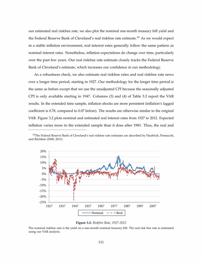
our estimated real riskfree rate, we also plot the nominal one-month treasury bill yield and

the Federal Reserve Bank of Cleveland’s real riskfree rate estimate.10 As we would expect

in a stable inflation environment, real interest rates generally follow the same pattern as

nominal interest rates. Nonetheless, inflation expectations do change over time, particularly

over the past few years. Our real riskfree rate estimate closely tracks the Federal Reserve

Bank of Cleveland’s estimate, which increases our confidence in our methodology.

As a robustness check, we also estimate real riskfree rates and real riskfree rate news

over a longer time period, starting in 1927. Our methodology for the longer time period is

the same as before except that we use the unadjusted CPI because the seasonally adjusted

CPI is only available starting in 1947. Columns (3) and (4) of Table 3.2 report the VAR

results. In the extended time sample, inflation shocks are more persistent (inflation’s lagged

coefficient is 0.78, compared to 0.07 before). The results are otherwise similar to the original

VAR. Figure 3.2 plots nominal and estimated real interest rates from 1927 to 2012. Expected

inflation varies more in the extended sample than it does after 1983. Thus, the real and

10The Federal Reserve Bank of Cleveland’s real riskfree rate estimates are described by Haubrich, Pennacchi,and Ritchken (2008, 2011).

-25%

-20%

-15%

-10%

-5%

0%

5%

10%

15%

20%

1927 1937 1947 1957 1967 1977 1987 1997 2007

Nominal Real

Figure 3.2: Riskfree Rate, 1927-2012

The nominal riskfree rate is the yield on a one-month nominal treasury bill. The real risk free rate is estimatedusing our VAR analysis.

111

nominal interest rates do not track each other as closely. Expected inflation is particularly

high in the 1930’s, 1940’s, and 1970’s, and deflation caused real interest rates to exceed

nominal interest rates in the 1920’s.

3.3.2 Cross-Sectional Equity Pricing

If real interest rate risk is priced and stocks vary in their exposure to real interest rate

risk, real interest rate risk should be priced in the cross section of stock returns. This is

not the first paper to connect time series interest rate changes with cross-sectional stock

returns. For example, Fama and French (1993) find comovement between excess stock

returns and excess returns on long term bonds but conclude that bond factors have little

impact on cross sectional stock prices. Petkova (2006) finds that innovations to term spreads

and one month nominal interest rates are correlated with and partially explain size and

value returns. Koijen, Lustig, and Van Nieuwerburgh (2012) find that high returns to value

stocks relative to growth stocks are explained by covariance with shocks to nominal bond

risk premia whereas returns to treasury bond portfolios of different maturities are largely

explained by differential exposure to the level of interest rates. Our empirical analysis

differs from previous studies because we focus specifically on stock exposure to real interest

rate innovations. Moreover, we sort stocks based on this exposure instead of focusing on

established size and value returns.

To test whether interest rate risk is priced we sort stocks into portfolios according to co-

variance with interest rate news (Newsh,t+1). Specifically, we estimate σih = covt (ri,t+1, Newsh,t+1)

on a rolling basis for all NYSE, AMEX, and NASDAQ common stocks using returns and

VAR Newsh estimates over the past three years, with the requirement that included stocks

must have at least two years of historical data. Value-weighted decile portfolios are formed

monthly by sorting stocks according to those estimates.

Table 3.3 reports market capitalization, average excess returns, and βih = σihσ2

hestimates

for each portfolio. The table also reports pricing errors (alphas) relative to the CAPM and

Fama and French (1993) three factor model and factor loadings (betas) for the three factor

112

Table 3.3: Real Riskfree Rate News Covariance Deciles

Value-weighted decile portfolios are formed at the end of each month by sorting stocks based on covariance withriskfree rate news over the past three years. The table reports betas with respect to riskfree rate news, averagesize, and average excess returns for each portfolio. The table also reports results for time series regressions ofexcess returns on excess market returns (the CAPM regression) and excess market returns, the Fama-Frenchsize factor (smb), and the Fama-French value factor (hml) (the 3 Factor regression). Standard errors for the 10-1portfolio difference are reported in parentheses. * represents 10% significance, ** represents 5% significance, ***represents 1% significance. The sample is NYSE, AMEX, and NASDAQ common stocks.

A. 1985-2012

Decile Rf News Market Cap Excess CAPM 3 Factor Factor Loadings (Betas)

Beta ($B) Return Alpha Alpha rmrf smb hml

1 -0.17 0.72 0.63% -0.19% -0.16% 1.27 0.61 -0.062 0.07 1.36 0.94% 0.24% 0.30% 1.10 0.22 -0.153 -0.04 1.94 0.87% 0.25% 0.23% 1.04 0.07 0.044 0.13 2.42 0.65% 0.06% 0.03% 1.00 -0.04 0.095 0.00 2.74 0.51% -0.03% -0.05% 0.94 -0.10 0.036 0.02 2.76 0.48% -0.06% -0.08% 0.93 -0.14 0.057 0.03 2.58 0.54% -0.02% -0.04% 0.97 -0.11 0.038 0.15 2.21 0.68% 0.06% 0.08% 1.04 -0.13 -0.079 0.14 1.69 0.61% -0.06% -0.04% 1.10 0.01 -0.06

10 0.41 0.85 0.21% -0.62% -0.44% 1.21 0.55 -0.47

10-1 0.58** 0.13** -0.42% -0.42% -0.27% -0.06 -0.07 -0.41***(0.23) (0.06) (0.33%) (0.34%) (0.34%) (0.08) (0.11) (0.12)

B. 1929-2012

Decile Rf News Market Cap Excess CAPM 3 Factor Factor Loadings (Betas)

Beta ($B) Return Alpha Alpha rmrf smb hml

1 -0.01 0.17 0.66% -0.05% -0.12% 1.15 0.52 -0.032 0.00 0.48 0.66% 0.04% 0.03% 1.04 0.20 -0.063 0.03 0.69 0.70% 0.13% 0.12% 0.99 0.08 -0.014 0.06 0.86 0.71% 0.15% 0.15% 0.96 0.02 0.005 0.01 0.98 0.60% 0.04% 0.02% 0.97 -0.03 0.066 0.03 1.05 0.56% -0.01% -0.03% 0.98 -0.03 0.097 0.06 1.08 0.58% -0.01% -0.02% 1.03 -0.08 0.088 0.06 1.05 0.56% -0.07% -0.10% 1.08 0.00 0.119 0.10 0.83 0.61% -0.07% -0.12% 1.15 0.04 0.17

10 0.11 0.38 0.58% -0.18% -0.27% 1.23 0.50 0.03

10-1 0.13 0.21*** -0.09% -0.13% -0.14% 0.07** -0.02 0.05(0.09) (0.02) (0.18%) (0.18%) (0.18%) (0.03) (0.06) (0.05)

113

model. Panel A reports results for our baseline 1985-2012 time period.11 Riskfree rate news

betas increase across the portfolios, and decile 10’s news beta is a significant 0.58 higher

than decile 1’s news beta. Monthly excess returns are 42 bps lower in the 10th decile than in

the 1st decile, but this return difference is not statistically significant, and there is no clear

pattern to excess returns across the decile portfolios other than a drop in returns in decile 10.

CAPM and 3 Factor alphas follow the same basic pattern. Factor loadings are also similar

across the portfolios. The one exception is that decile 10 has a large negative loading on

the value factor (hml). The bottom line is that there is no evidence that interest rate risk is

priced in the cross section of equities.

Results are similar in the extended 1929-2012 sample, reported in Panel B. Once again,

average excess returns and alpha estimates decrease with interest rate news exposure, but

the differences are not significant. The most striking difference between Panel A and Panel

B is that βih differences across the portfolios are not significant in the extended sample.

This suggests that stock-level interest rate risk was not stable over time early in the sample,

undercutting our ability to form interest rate risk portfolios. This problem appears to be

concentrated in the first few decades of the sample when inflation and interest rates were

most volatile. In later analysis, we examine a 1952 to 2012 sample and find significant βih

differences between the decile portfolios. As in the other samples, these βih differences are

not accompanied by significant return differences.

3.3.3 Equity Premium

Because the market portfolio is a claim to future dividends, it may be exposed to interest

rate risk. Thus, interest rate risk may affect expected equity returns and could explain part

of the equity premium puzzle. The magnitude and direction of this effect depend on the

market return’s covariance with interest rate news and the price of interest rate risk.

AER make the extreme claim that interest rate risk explains virtually all of the equity

11We form the portfolios based on at least two years of historical data, which causes the sample to start in1985 instead of 1983.

114

premium. In their model, assets are priced based on covariance with consumption growth

shocks and time preference shocks, which map directly into interest rate shocks. Consistent

with previous studies, they estimate that equity returns are essentially uncorrelated with

consumption growth. Thus, their explanation of the equity premium is almost entirely based

on interest rate risk. Equities are risky because they have a long duration and are sensitive

to persistent real interest rate shocks. Duration simultaneously explains the upward sloping

yield curve and the equity premium. In the AER benchmark model, equity returns are

highly sensitive to interest rate shocks, with a correlation of approximately -0.92. Moreover,

their benchmark model implies that equity returns have an interest rate news beta of -1.12

Using our estimates of interest rate news, we can directly measure these two moments.

Panel A of Table 3.4 shows results for the 1985 to 2012 time period. Excess market returns

(rmr f ) have a correlation of 0.05 and a beta of 0.11 with respect to interest rate news. These

estimates are close to zero, suggesting that equity returns have little exposure to interest

rate risk. According to the point estimate, the market return is positively correlated with

interest rate shocks, consistent with long run consumption growth shocks and in contrast to

AER’s time preference shocks.

Table 3.4 also reports interest rate correlations and betas for the long-short decile 10

minus decile 1 interest rate risk portfolio and for 1 to 2 year and 5 to 10 year bonds.13

By construction, the long-short interest rate risk portfolio has a positive beta. The bond

portfolios have negative exposures to interest rate news. However, these exposures are small.

Interest rate betas are -0.04 for both portfolios, and the beta is only significantly different

from zero for the short-term bonds.

The final rows of Table 3.4 report average excess returns and average excess returns

divided by interest rate news beta. If interest rate news is the primary risk factor investors

care about, this ratio (the implied price of beta) should be consistent across assets. The point

12The high negative correlation comes from AER’s Table 3 estimate that interest rate shocks are relativelylarge and persistent while dividend variance is low. The beta of -1 is implied by AER’s benchmark assumptionthat real dividend growth is independent of real interest rates.

13Bond return data is from CRSP.

115

Table 3.4: Equity Market and Bond Real Interest Rate Risk

rmrf is the excess return on the CRSP value weighted market portfolio. Decile 10-1 is returns to long-shortportfolio representing the difference between the 10th and first riskfree rate news covariance portfolios, describedin Table 2. 1-2 and 5-10 year bonds represent excess returns to treasury bonds of those durations, as calculatedby CRSP. Correlations and betas with respect to riskfree rate news and average returns are reported for eachreturn series. The price of beta is defined as average returns divided by beta. Standard errors are reportedin parentheses. Standard errors for the price of beta are calculated using the delta method. * represents 10%significance, ** represents 5% significance, *** represents 1% significance.

A. 1985-2012

1-2 Year 5-10 Yearrmrf Decile 10-1 Bonds Bonds

Rf News 0.04 0.14** -0.14*** -0.03Correlation (0.05) (0.05) (0.05) (0.05)

Rf News 0.11 0.58** -0.04*** -0.04Beta (0.17) (0.23) (0.02) (0.06)

Average 0.60%** -0.42% 0.12%*** 0.34%***Excess Returns (0.25%) (0.33%) (0.02%) (0.09%)

Price of 5.35% -0.72%** -3.14%*** -9.70%Beta (10.57%) (0.30%) (0.64%) (13.81%)

B. 1952-2012

1-2 Year 5-10 Yearrmrf Decile 10-1 Bonds Bonds

Rf News 0.05 0.12*** -0.40*** -0.12***Correlation (0.04) (0.04) (0.03) (0.04)

Rf News 0.10 0.30*** -0.12*** -0.10***Beta (0.08) (0.09) (0.01) (0.03)

Average 0.55%*** -0.16% 0.09%*** 0.16%***Excess Returns (0.16%) (0.19%) (0.02%) (0.06%)

Price of 5.43% -0.54% -0.72%*** -1.57%***Beta (5.91%) (0.46%) -(0.12%) -(0.13%)

116

estimates clearly differ. In particular, the bond returns and cross-sectional interest rate risk

portfolio imply a negative price of interest rate risk whereas market returns imply a positive

price. Unfortunately, betas and average returns are measured too imprecisely to definitively

rule out consistent interest rate risk pricing across the assets.

Panel B of Table 3.4 reports the same statistics for a longer sample period, starting in

1952 when CRSP bond return data starts. The basic results are all the same.

Our findings suggest that interest rate risk is unlikely to explain the equity premium.

Certainly, there is no evidence in favor of the hypothesis that equities face significant interest

rate risk. How can this be reconciled with AER’s empirical findings? The main difference

between our analysis and AER’s is that AER do not estimate real interest rate innovations.

Their GMM includes the unconditional correlation between equity returns and the real risk

free rate at an annual frequency but omits the more important correlation of interest rate

news with excess equity returns. Our analysis estimates this moment and finds that it is

essentially zero.

3.4 Conclusion

Is real interest rate risk priced? Theoretically, it could be priced in either direction. Empiri-

cally, there is little evidence that real interest rate risk is priced at all.

Our interest rate risk model has two theoretical implications. First, it matters where

interest rate shocks comes from. Interest rate increases stemming from news about future

consumption growth are generally good news to investors whereas interest rate increases

stemming from time preference shocks are generally bad news. Thus, long-run consumption

risk logic implies that long-duration assets are relatively safe whereas time preference risk

logic implies that long-duration assets are relatively risky. A more general lesson is the

importance of thinking in general equilibrium terms. Because interest rates are endogenous,

interest rate risk is not a meaningful concept without specifying what is driving interest

rate shocks.

The second theoretical implication of our model is that Epstein-Zin preferences with

117

ψ close to 1 and significantly different from 1/γ imply implausible aversion to future

time preference shocks. If we take Epstein-Zin utility seriously as a description of actual

preferences, this undermines many popular calibrations, such as those proposed by Bansal

and Yaron (2004).

Empirically, stocks sorted on interest rate risk have only small, statistically insignificant

return differences. Moreover, the market return and treasury bond returns have low

covariance with interest rate news. Thus, interest rate risk is unlikely to explain much of

equity or bond return premia even if it is priced to some extent in the cross section. Overall,

our results suggest that interest rate risk is not a major concern to investors.

118

References

Adelino, M., Gerardi, K. and Willen, P. S. (2011a). What Explains Differences in Fore-closure Rates? A Response to Piskorski , Seru , and Vig. Federal Reserve Bank of Atlantaworking paper.

—, — and — (2011b). Why Don’t Lenders Renegotiate More Home Mortgages? Redefaults,Self-Cures and Securitization. Federal Reserve Bank of Atlanta working paper.

Agarwal, S., Amromin, G., Ben-David, I., Chomsisengphet, S. and Evanoff, D. D. (2011).The role of securitization in mortgage renegotiation. Journal of Financial Economics, 102 (3),559–578.

—, —, —, —, Piskorski, T. and Seru, A. (2012a). Policy Intervention in Debt Renegotiation:Evidence from the Home Affordable Modification Program. Working paper.

—, Chang, Y. and Yavas, A. (2012b). Adverse Selection in Mortgage Securitization. Journalof Financial Economics, 105 (3), 640–660.

Akerlof, G. A. (1970). The Market for "Lemons": Quality Uncertainty and the MarketMechanism. The Quarterly Journal of Economics, 84 (3), 488–500.

Albuquerque, R., Eichenbaum, M. and Rebelo, S. (2012). Valuation Risk and Asset Pricing.Working paper.

Amihud, Y. (2002). Illiquidity and stock returns: cross-section and time-series effects. Journalof Financial Markets, 5 (1), 31–56.

Angrist, J. and Pischke, J.-S. (2009). Mostly Harmless Econometrics: An Empiricist’s Companion.Princeton, NJ: Princeton University Press.

Bai, J., Philippon, T. and Savov, A. (2012). Have Financial Markets Become More Informa-tive? Working paper.

Bajaj, V. (2007). For Some Subprime Borrowers, Few Good Choices.

Baker, M. and Stein, J. C. (2004). Market liquidity as a sentiment indicator. Journal ofFinancial Markets, 7 (3), 271–299.

Bansal, R. and Yaron, A. (2004). Risks for the Long Run: A Potential Resolution of AssetPricing Puzzles. The Journal of Finance, LIX (4), 1481–1509.

119

Barber, B. M. and Odean, T. (2000). Trading Is Hazardous to Your Wealth: The CommonStock Investment Performance of Individual Investors. The Journal of Finance, LV (2),773–806.

Bernard, V. L. and Thomas, J. K. (1989). Post-Earnings-Announcement Drift: Delayed PriceResponse or Risk Premium? Journal of Accounting Research, 27, pp. 1–36.

Bernstein, S. (2012). Does Going Public Affect Innovation? Working paper.

Biais, B., Glosten, L. and Spatt, C. (2005). Market microstructure: A survey of micro-foundations, empirical results, and policy implications. Journal of Financial Markets, 8 (2),217–264.

Bolton, P. and Scharfstein, D. S. (1996). Optimal Debt Structure and the Number ofCreditors. Journal of Political Economy, 104 (1), 1–25.

Brunnermeier, M. K., Simsek, A. and Xiong, W. (2012). A Welfare Criterion for Modelswith Distorted Beliefs. Working paper.

Bubb, R. and Kaufman, A. (2013). Securitization and Moral Hazard: Evidence from CreditScore Cutoff Rules. Working paper.

Calem, P., Covas, F. and Wu, J. (2011). The Impact of a Liquidity Shock on Bank Lending:The Case of the 2007 Collapse of the Private-Label RMBS Market. Working paper.

Campbell, J. Y. (1993). Intertemporal Asset Pricing without Consumption Data. The AmericanEconomic Review, 83 (3), 487–512.

— (1996). Understanding Risk and Return. Journal of Political Economy, 104 (2), 298–345.

—, Giglio, S. and Pathak, P. (2011). Forced Sales and House Prices. American EconomicReview, 101 (5), 2108–2131.

— and Viceira, L. M. (2003). Strategic Asset Allocation: Portfolio Choice for Long-Term Investors.Oxford University Press.

Chordia, T., Roll, R. and Subrahmanyam, A. (2000). Commonality in liquidity. Journal ofFinancial Economics, 56 (1), 3–28.

CoreLogic (2013). National Foreclosure Report for April 2013. (April).

Credit Suisse (2007). The Day After Tomorrow: Payment Shock and Loan Modifications.(April 5).

Dang, T. V., Gorton, G. and Holmström, B. (2009). Ignorance and the Optimality of Debtfor the Provision of Liquidity. Working paper.

Daniel, K., Hirshleifer, D. and Subrahmanyam, A. (1998). Investor Psychology andSecurity Market Under- and Overreactions. The Journal of Finance, 53 (6), 1839–1885.

120

DeBondt, W. F. and Thaler, R. H. (1995). Financial Decision Making in Markets and Firms:A Behavioral Perspective. In R. Jarrow, V. Maksimovic and W. Ziemba (eds.), Finance,Elsevier - North Holland: Series of Handbooks in Operations Research and ManagementSciences.

Diamond, D. W. and Verrecchia, R. E. (1981). Information aggregation in a noisy rationalexpectations economy. Journal of Financial Economics, 9 (3), 221–235.

Epstein, L. G., Farhi, E. and Strzalecki, T. (2013). How Much Would You Pay to ResolveLong-Run Risk? Working paper.

— and Zin, S. E. (1991). Substitution, Risk Aversion, and the Temporal Behavior of Con-sumption and Asset Returns: An Empirical Analysis. Journal of Political Economy, 99 (2),263–286.

Fama, E. F. (1970). Fama_1970.pdf. 1American Economic Review, 60 (1), 163–174.

— and French, K. R. (1992). The Cross-Section of Expected Stock Returns. The Journal ofFinance, 47 (2), 427–465.

— and — (1993). Common risk factors in the returns on stocks and bonds. Journal of FinancialEconomics, 33 (1), 3–56.

Fannie Mae (2006). 2006 Servicing Guide.

Frazzini, A. and Lamont, O. (2007). The Earnings Announcement Premium and TradingVolume. Working paper.

Fuster, A. and Vickery, J. (2013). Securitization and the Fixed-Rate Mortgage. Workingpaper.

Gervais, S. and Odean, T. (2001). Learning to be overconfident. Review of Financial Studies,14 (1), 1–27.

Glosten, L. R. and Milgrom, P. R. (1985). Bid, ask and transaction prices in a specialistmarket with heterogeneously informed traders. Journal of Financial Economics, 14 (1),71–100.

Gorton, G. and Metrick, A. (2012). Securitized banking and the run on repo. Journal ofFinancial Economics, 104 (3), 425–451.

Grossman, S. (1976). On the Efficiency of Competitive Stock Markets Where Trades HaveDiverse Information. The Journal of Finance, 31 (2), 573–585 CR – Copyright © 1976American Financ.

Grossman, S. J. and Hart, O. D. (1986). The Costs and Benefits of Ownership: A Theory ofVertical and Lateral Integration. Journal of Political Economy, 94 (4), 691–719.

— and Stiglitz, J. E. (1980). On the Impossibility of Informationally Efficient Markets. TheAmerican Economic Review, 70 (3), 393–408.

121

Harris, M. and Raviv, A. (1993). Differences of Opinion Make a Horse Race. Review ofFinancial Studies, 6 (3), 473–506.

Hart, O. and Moore, J. (1990). Property Rights and the Nature of the Firm. Journal ofPolitical Economy, 98 (6), 1119–1158.

Haubrich, J., Pennacchi, G. and Ritchken, P. (2008). Estimating Real and Nominal TermStructures using Treasury Yields, Inflation, Inflation Forecasts, and Inflation Swap Rates.Working paper.

—, — and — (2011). Inflation Expectations, Real Rates, and Risk Premia: Evidence fromInflation Swaps. Working paper.

Hellwig, M. F. (1980). On the aggregation of information in competitive markets. Journal ofEconomic Theory, 22 (3), 477–498.

Hodrick, R. J. and Prescott, E. C. (1997). Postwar U.S. Business Cycles: An EmpiricalInvestigation. Journal of Money, Credit and Banking, 29 (1), 1–16.

Holmström, B. (2008). Discussion of ’The Panic of 2007,’ by Gary Gorton. Working paper.

Holmstrom, B. and Milgrom, P. (1991). Multitask Principal-Agent Analyses: IncentiveContracts, Asset Ownership, and Job Design. Journal of Law, Economics, & Organization, 7,24–52.

Holtz-Eakin, D., Newey, W. and Rosen, H. S. (1988). Estimating Vector Autoregressionswith Panel Data. Econometrica, 56 (6), 1371–1395.

Hong, H. and Stein, J. C. (1999). A Unified Theory of Underreaction, Momentum Trading,and Overreaction in Asset Markets. The Journal of Finance, 54 (6), 2143–2184.

— and — (2007). Disagreement and the Stock Market. Journal of Economic Perspectives, 21 (2),109–128.

Hunt, J. P. (2009). What Do Subprime Securitization Contracts Actually Say About LoanModification? Preliminary Results and Implications. Working paper.

Inside Mortgage Finance (2008). The Mortgage Market Statistical Annual for 2008. Bethesda,MD: Inside Mortgage Finance Publications.

Jegadeesh, N. and Titman, S. (1993). Returns to Buying Winners and Selling Losers:Implications for Stock Market Efficiency. The Journal of Finance, 48 (1), 65–91.

Jensen, M. C. and Meckling, W. H. (1976). Theory of the firm: Managerial behavior, agencycosts and ownership structure. Journal of Financial Economics, 3 (4), 305–360.

Jiang, W., Nelson, A. and Vytlacil, E. (2010). Securitization and Loan Performance: AContrast of Ex Ante and Ex Post Relations in the Mortgage Market. Working paper.

Kacperczyk, M. and Schnabl, P. (2010). When Safe Proved Risky: Commercial Paper duringthe Financial Crisis of 2007-2009. Journal of Economic Perspectives, 24 (1), 29–50.

122

Kandel, E. and Pearson, N. D. (1995). Differential Interpretation of Public Signals andTrade in Speculative Markets. Journal of Political Economy, 103 (4), 831–872.

Keys, B. J., Mukherjee, T., Seru, A. and Vig, V. (2010). Did Securitization Lead to LaxScreening? Evidence from Subprime Loans. The Quarterly Journal of Economics, 125 (1),307–362.

Koijen, R. S., Lustig, H. and Van Nieuwerburgh, S. (2012). The Cross-Section and Time-Series of Stock and Bond Returns. Working paper.

Kyle, A. S. (1985). Continuous Auctions and Insider Trading. Econometrica: Journal of theEconometric Society, 53 (6), 1315–1335.

—, Obizhaeva, A. A. and Wang, Y. (2013). Smooth Trading with Overconfidence and MarketPower. Working paper.

— and Wang, F. A. (1997). Speculation Duopoly with Agreement to Disagree: Can Overcon-fidence Survive the Market Test? The Journal of Finance, 52 (5), 2073–2090.

Lakonishok, J., Shleifer, A. and Vishny, R. W. (1994). Contrarian Investment, Extrapolation,and Risk. The Journal of Finance, 49 (5), 1541–1578.

Levitin, A. J. and Twomey, T. (2011). Mortgage Servicing. Yale Journal on Regulation, 28, 1–90.

Loutskina, E. (2011). The role of securitization in bank liquidity and funding management.Journal of Financial Economics, 100 (3), 663–684.

— and Strahan, P. E. (2009). Securitization and the Declining Impact of Bank Finance onLoan Supply: Evidence from Mortgage Originations. The Journal of Finance, 64 (2), 861–889.

Mayer, C. (2009). Testimony of Dr. Christopher J. Mayer.

Merton, R. C. (2013). An Intertemporal Capital Asset Pricing Model. Econometrica, 41 (5),867–887.

Mian, A. and Sufi, A. (2009). The Consequences of Mortgage Credit Expansion: Evidencefrom the U.S. Mortgage Default Crisis. The Quarterly Journal of Economics, 124 (4), 1449–1496.

Milgrom, P. and Stokey, N. (1982). Information, trade and common knowledge. Journal ofEconomic Theory, 26 (1), 17–27.

Odean, T. (1998). Volume , Volatility , Price , and Profit When All Traders Are AboveAverage. The Journal of Finance, 53 (6), 1887–1934.

Peng, L. and Xiong, W. (2006). Investor attention, overconfidence and category learning.Journal of Financial Economics, 80 (3), 563–602.

Petkova, R. (2006). Do the Fama-French Factors Proxy for Innovations in Predictive Vari-ables? The Journal of Finance, 61 (2), 581–612.

123

Piskorski, T., Seru, A. and Vig, V. (2010). Securitization and distressed loan renegotiation:Evidence from the subprime mortgage crisis. Journal of Financial Economics, 97 (3), 369–397.

Posner, E. A. and Zingales, L. (2009). A Loan Modification Approach to the Housing Crisis.American Law and Economics Review, 11 (2), 575–607.

Rajan, U., Seru, A. and Vig, V. (2010). The Failure of Models That Predict Failure: Distance,Incentives and Defaults. Working paper.

Rubinstein, M. (2001). Rational markets: Yes or no? The affirmative case. Financial AnalystsJournal, 57 (3), 15–29.

Sadka, R. and Scherbina, A. (2007). Analyst Disagreement, Mispricing, and Liquidity. TheJournal of Finance, 62 (5), 2367–2403.

Stanton, R. and Wallace, N. (2011). The Bear’s Lair: Index Credit Default Swaps and theSubprime Mortgage Crisis. Review of Financial Studies, 24 (10), 3250–3280.

Statman, M., Thorley, S. and Vorkink, K. (2006). Investor Overconfidence and TradingVolume. Review of Financial Studies, 19 (4), 1531–1565.

Stock, J. H. and Watson, M. W. (1999). Forecasting Inflation. National Bureau of EconomicResearch Working Paper Series, No. 7023.

Vayanos, D. and Wang, J. (2009). Liquidity and Asset Prices: A Unified Framework. Workingpaper.

Weil, P. (1989). The Equity Premium Puzzle and the Risk-free Rate Puzzle. Journal ofMonetary Economics, 24 (3), 401–421.

Wooldridge, J. M. (2002). Econometric Analysis of Cross Section and Panel Data. Cambridge,Mass.: MIT Press.

124

Appendix A

Appendix to Chapter 1

A.1 Modification Algorithm

The LPS dataset lacks an explicit modification flag but contains enough detailed panel

information to identify changes to loan terms over time. My loan modification algorithm

differs in a few details but is essentially the same as the algorithm employed by Adelino,

Gerardi, and Willen (2011b). The purpose of the algorithm is to identify changes to loan

terms that are consistent with modification and do not have other likely explanations. Some

changes are enough to identify a modification on their own. For example, absent errors in

the data, an interest rate change to a fixed rate loan must stem from modification. Other

changes require confirmatory evidence. For example, a principal reduction could be from

a modification or from a prepayment. The size of the reduction, changes in monthly

payments, and other simultaneous modifications all inform whether the reduction stems

from a modification. In all cases, the loans in question are seriously delinquent at the time

of the potential modification, adding to the likelihood that the algorithm is identifying true

modifications. The algorithm separately identifies four types of modifications: interest

rate reductions, term extensions, principal decreases, and principal increases. These

modifications are not mutually exclusive and often take place simultaneously. I consider a

loan to be modified if the algorithm flags it with any of the four modification types.

125

A.1.1 Interest Rate Reductions

Interest rate reductions are easiest to identify in fixed-rate loans and adjustable-rate loans

that are still in their introductory fixed-rate period. For these loans, I define an interest

rate reduction as a change that reduces a loan’s interest rate to at least 0.5 ppt below the

previous month’s rate and the loan’s origination interest rate.

For adjustable-rate mortgages, I first compute a fully indexed interest rate for each loan

in each month using LPS data on the loan’s reference index and spread combined with

time-series data on the index rates. For example, a loan that references LIBOR and has a

spread of 2 ppt would have a fully indexed rate of LIBOR + 2 ppt in any month. I abstract

from details on exactly how frequently rates reset and consider any loan to be adjustable

if it is past or within 2 months of the end of its introductory period. To be flagged as an

interest rate reduction, a loan’s interest rate must decrease to at least 0.5 ppt below the

previous month’s rate, the origination interest rate, and the fully indexed rate.

A.1.2 Term Extensions

To be flagged as a term extension, a loan’s remaining term to maturity must increase by

at least 20 months or rise above its initial term to maturity. The term change must also

be contemporaneous with a monthly payment decrease, principal increase, or explicit loss

mitigation flag in the data.

A.1.3 Principal Decreases

To be flagged as a principal decrease, the mortgage must have had outstanding principal

of at least $25K in the previous month, and the principal balance must have decreased by

between 10% and 30% and be accompanied by a payment decrease or term extension. The

10-30% range is used to differentiate modifications from scheduled principal decreases and

prepayments. Adelino, Gerardi, and Willen (2011b) experiment with the 30% cutoff and

find that results are not sensitive to its exact value.

126

A.1.4 Principal Increases

To be flagged as a principal increase, principal must increase by at least 1% (0.5% for

option ARM mortgages) and be accompanied by either a payment increase or a term length

decrease.

A.2 Supplemental Figures and Tables

0

200

400

600

800

1,000

Ori

gina

tion

Am

ount

($K

)

Origination Month (2007)

Jumbo Loans Non-Jumbo Loans

Figure A.1: Origination Amount by Origination Month

Mean loan origination amounts for sample jumbo and non-jumbo loans.

127

710

715

720

725

730

735

740

745F

ICO

Sco

re



Figure A.2: FICO Score by Origination Month

Mean FICO scores for sample jumbo and non-jumbo loans.

0.6

0.65

0.7

0.75

0.8

Loa

n t

o V

alue

Rat

io



Figure A.3: Loan to Value Ratio by Origination Month

Mean loan to value ratios for sample jumbo and non-jumbo loans.

128

0%

20%

40%

60%

80%

100%F

ull

In

com

e D

ocu

men

tati

on



Figure A.4: Income Documentation by Origination Month

Percent of sample jumbo and non-jumbo loans with full income documentation.

5.85.9

66.16.26.36.46.56.66.76.86.9

Ori

gin

al I

nter

est

Rat

e (%

)



Figure A.5: Original Interest Rate by Origination Month

Mean original interest rates for sample jumbo and non-jumbo loans.

129

Table A.1: Additional Robustness Checks

Regressions are the same as Kruger’s (2013) baseline IV regressions (Table 4, columns 2-4) except where noted.Columns 1-3 of Panel A drop loan characteristic controls. Columns 4-6 of Panel A add back loans transferred tonon-LPS servicers, which were previously dropped from the sample. Panel B control for originination-monthfixed effects using non-jumbo loans without controlling for the interaction between private securitization andnon-jumbo status. R-squared statistics are calculated within MSAs. Clustered (by MSA) standard errors are inparentheses. * represents 10% significance, ** represents 5% significance, *** represents 1% significance.

A. Regressions without loan characteristic controls (1-3) and with transferred loans (4-6)

(1) (2) (3) (4) (5) (6)IV IV IV IV IV IV


Mean 0.695 0.135 0.052 0.695 0.135 0.052

Privately Securitized 0.055*** 0.030** -0.039*** 0.063*** 0.051*** -0.032***(0.016) (0.012) (0.010) (0.015) (0.012) (0.009)

Loan Characteristics No No No Yes Yes YesDelinquency Month FE Yes Yes Yes Yes Yes YesOrigination Month FE No No No No No NoMSA FE Yes Yes Yes Yes Yes Yes

Origination Months Jan-Aug Jan-Aug Jan-Aug Jan-Aug Jan-Aug Jan-AugInclude Non-Jumbo Loans No No No No No No

Observations 15,945 15,945 7,893 17,165 17,165 8,556Adusted R-Squared 0.036 0.011 -0.002 0.079 0.027 0.088

B. Non-jumbo origination month control regressions without securitization*non-jumbo interaction

(1) (2) (3)IV IV IV


Mean 0.695 0.135 0.052

Privately Securitized 0.172*** 0.079*** -0.050**(0.031) (0.018) (0.022)

Loan Characteristics Yes Yes YesDelinquency Month FE Yes Yes YesOrigination Month FE Yes Yes YesMSA FE Yes Yes Yes

Origination Months Jan-Aug Jan-Aug Jan-AugInclude Non-Jumbo Loans Yes Yes Yes


130

Appendix B


B.1 General Model Derivations and Proofs

B.1.1 Solution

I assume that the price function is linear:

P = α + βy− γ (X− µX) (B.1)

Claim 1. β 6= 0.

Proof. Assume β = 0. Thus, price is uninformative about private signals, and all agents have

posterior beliefs of Ei[θ|ym(i), xm(i), P] =τpµ+ψτsym(i)

τp+ψτsand Vari[θ|ym(i), xm(i), P] =

(τp + ψτs

)−1,

resulting in asset demand Di

[ym(i), xm(i), P

]=

Ei [θ|ym(i),xm(i),P]−PNη Vari [θ|ym(i),xm(i),P]

= ηN

[τpµ + ψτsym(i) −

(τp + ψτs

)P].

Solving ∑i Di = X for the market clearing price implies P =τpµ+ψτs y− X

η

τp+ψτs. Thus, β = ψτs

τp+ψτs6=

0, a contradiction.

Given the price function described by equation (B.1), agent i extracts a noisy signal for

y−m(i) from observing price, ym(i), and xm(i):

Am(i) =M

β (M− 1)(P− α)− 1

M− 1ym(i) +

γMβ (M− 1)

(xm(i) −

µX

M

)= y−m(i) −

γMβ

(x−m(i) −

µX

M

)(B.2)

131

Note that Am(i) ∼i N(

θ, 1(M−1)τs

+(

γβ

)2M

M−1 V)

and Am(i) is independent of ym(i) and

xm(i). Using Bayesian updating with signals ym(i) and Am(i) and substituting P, ym(i), xm(i)

for Am(i) using (B.2), agent i’s posterior beliefs as a function of P, ym(i), xm(i) are:

Ei[θ|ym(i), xm(i), P] =

τpµ− MτAβ(M−1)α +

(ψτs − τA

M−1

)ym(i)

+ γMτAβ(M−1)

(xm(i) −

µXM

)+ MτA

β(M−1)P

τp + ψτs + τA

(B.3a)

Vari[θ|ym(i), xm(i), P] =(τp + ψτs + τA

)−1 (B.3b)

where τA =

(1

(M−1)τs+(

γβ

)2M

M−1 V)−1

is the precision agent i attributes to Am(i).

Agent i’s asset demand is:

Di =Ei[θ|ym(i), xm(i), P]− PNη Vari[θ|ym(i), xm(i), P]

=η

N

τpµ− MτAβ(M−1)α +

(ψτs − τA

M−1

)ym(i) +

γMτAβ(M−1)

(xm(i) −

µXM

)−(

τp + ψτs +(

1− Mβ(M−1)

)τA

)P

(B.4)

The market clearing price must solve X = ∑i Di. Thus,

P =τpµ− 1

η µX − MτAβ(M−1)α +

(ψτs − τA

M−1

)y−

(1η −

γτAβ(M−1)

)(X− µX)

τp + ψτs +(

1− Mβ(M−1)

)τA

(B.5)

Equations (B.1) and (B.5) yield the following system of equations:α

β

γ

(

τp + ψτs +

(1− M

β (M− 1)

)τA

)=

τpµ− 1

η µX − MτAβ(M−1)α

ψτs − τAM−1

1η −

γτAβ(M−1)

(B.6)

Claim 2. The unique solution to equations (B.6) is:

α =


)µ−

(ηψ2τs +

MVη

)µX


)+(τp + ψτs

)MV

(B.7)

β =ψτs

(η2ψ (M + ψ− 1) τs + MV

)η2ψ2τs

(τp + (M + ψ− 1) τs

)+(τp + ψτs

)MV

(B.8)

γ =η2ψ (M + ψ− 1) τs + MV

η(η2ψ2τs

(τp + (M + ψ− 1) τs

)+(τp + ψτs

)MV

) (B.9)

132

Proof. Consider Γ ≡ γβ . We already established that β 6= 0 so Γ is finite. Substituting Γ into

(B.6) and dividing the γ equation by the β equation yields:

Γ =

1η − Γ τA

M−1

ψτs − τAM−1

=1

ηψτs(B.10)

Plugging (B.10) into the β equation of (B.6) yields:

β =ψτs

(η2ψ (M + ψ− 1) τs + MV

)η2ψ2τs

(τp + (M + ψ− 1) τs

)+(τp + ψτs

)MV

(B.11)

Plugging (B.10) and (B.11) into the γ equation of (B.6) yields:

γ =η2ψ (M + ψ− 1) τs + MV

η(η2ψ2τs

(τp + (M + ψ− 1) τs

)+(τp + ψτs

)MV

) (B.12)

Finally, plugging (B.10), (B.11), and (B.12) into the α equation of (B.6) yields:

α =


)µ−

(ηψ2τs +

MVη

)µX


)+(τp + ψτs

)MV

(B.13)

B.1.2 Trading

Using equation (B.4),

Tradem ≡ ∑i:m(i)=m

[Di −

MN

xm

]=

{η

M

(ψτs −

τA

M− 1

)(ym − y)

}−{(

1− ηγτA

(M− 1) β

)(xm − x)

}(B.14)

All other trading derivations are in the main text of the paper.

B.1.3 Liquidity

Recall that illiquidity is defined as:

λ ≡dP

dym

dTrademdym

133

Taking derivatives of P (eq. B.1) and Tradem (eq. B.14) with respect to ym and plugging in γ

from (B.9) and Γ from (B.10) yields:

λ =−γ( N

M

) ( ηN

) ( γMτAβ(M−1) + γ

(τp + ψτs +

(1− M

β(M−1)

)τA

))− 1

=M(η2ψ2τs + MV

) (η2ψ (M + ψ− 1) τs + MV

)η (M− 1) (η2 (ψ2 − ψ) τs + MV)

(η2ψ2τs

(τp + (M + ψ− 1) τs

)+(τp + ψτs

)MV

)=

{M

(M− 1) η(τp + ψτs + τA

)}

+

{η2ψ2τs

η2ψ2τs + MV

}{τs

τp + ψτs + τA

}{η

M

(ψτs −

β

M(τp + ψτs + τA

))}−1

= {S}+ {B1} {B2} {B3}−1 (B.15)

Consistent with the baseline model, limV→0dλdψ < 0, limV→0

dλdτs

< 0, and limV→0dλdτp

< 0.

From (B.15) one can see that dλdτp

< 0 for all V. However, dλdψ and dλ

dτsare not always negative.

Their signs are determined by complicated functions of the parameters. Considering limiting

cases is instructive. We have already seen that dλdψ and dλ

dτsare negative in the limit as V → 0.

Both are also negative in the limit as V → ∞. For interim values of V (i.e., positive, finite V),

dλdψ and dλ

dτscan be positive or negative. Both follow a similar pattern. As ψ→ 0 or τs → 0,

λ→ M(M−1)ητp

, which is solely a supply impact – it includes no belief price response.1,2 dλdψ

and dλdτs

initially have the same sign as η2τp−V (i.e., sign[limψ→0

dλdψ

]= sign

[limτs→0

dλdτs

]=

sign[η2τp −V

]). As ψ and τs increase, they eventually decrease λ, driving it to approach

zero as ψ→ ∞ or τs → ∞.

1Though I restrict my attention to overconfidence (ψ > 1) in other parts of the paper, it is useful to generalizeand consider underconfidence (ψ < 1) here to get a full picture of the relationship between λ and ψ.

2The total risk tolerance of agents not receiving the shock is (M−1)ηM and their posterior variance is τ−1

p .

134

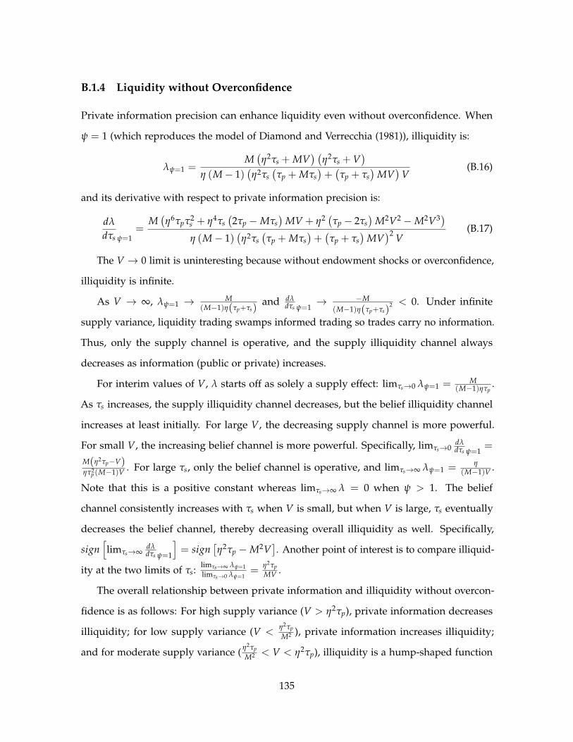
B.1.4 Liquidity without Overconfidence

Private information precision can enhance liquidity even without overconfidence. When

ψ = 1 (which reproduces the model of Diamond and Verrecchia (1981)), illiquidity is:

λψ=1 =M(η2τs + MV

) (η2τs + V

)η (M− 1)

(η2τs

(τp + Mτs

)+(τp + τs

)MV

)V

(B.16)

and its derivative with respect to private information precision is:

dλ

dτs ψ=1=

M(η6τpτ2

s + η4τs(2τp −Mτs

)MV + η2 (τp − 2τs

)M2V2 −M2V3)

η (M− 1)(η2τs

(τp + Mτs

)+(τp + τs

)MV

)2 V(B.17)

The V → 0 limit is uninteresting because without endowment shocks or overconfidence,

illiquidity is infinite.

As V → ∞, λψ=1 → M(M−1)η(τp+τs)

and dλdτs ψ=1

→ −M(M−1)η(τp+τs)

2 < 0. Under infinite

supply variance, liquidity trading swamps informed trading so trades carry no information.

Thus, only the supply channel is operative, and the supply illiquidity channel always

decreases as information (public or private) increases.

For interim values of V, λ starts off as solely a supply effect: limτs→0 λψ=1 = M(M−1)ητp

.

As τs increases, the supply illiquidity channel decreases, but the belief illiquidity channel

increases at least initially. For large V, the decreasing supply channel is more powerful.

For small V, the increasing belief channel is more powerful. Specifically, limτs→0dλdτs ψ=1

=

M(η2τp−V)ητ2

p (M−1)V . For large τs, only the belief channel is operative, and limτs→∞ λψ=1 = η(M−1)V .

Note that this is a positive constant whereas limτs→∞ λ = 0 when ψ > 1. The belief

channel consistently increases with τs when V is small, but when V is large, τs eventually

decreases the belief channel, thereby decreasing overall illiquidity as well. Specifically,

sign[limτs→∞

dλdτs ψ=1

]= sign

[η2τp −M2V

]. Another point of interest is to compare illiquid-

ity at the two limits of τs:limτs→∞ λψ=1limτs→0 λψ=1

=η2τpMV .

The overall relationship between private information and illiquidity without overcon-

fidence is as follows: For high supply variance (V > η2τp), private information decreases

illiquidity; for low supply variance (V <η2τp

M2 ), private information increases illiquidity;

and for moderate supply variance ( η2τp

M2 < V < η2τp), illiquidity is a hump-shaped function

135

of private information. Within the moderate case, τs decreases illiquidity overall when

V >η2τp

M and increases illiquidity overall when V <η2τp

M .

136

B.2 Supplemental Tables

Table B.1: Stock VAR Results

turn and illiq are detrended log turnover and illiq (a measure of illliquidity), respectively. rmrf is the excessreturn of the CRSP value weighted market return over the risk free rate. turn and illiq were detrended using aHodrick and Prescott (1997) filter with a penalty value of 14,400. Reported results are for a 2-lag VAR of turn,illiq, and rmrf. Bootstrapped standard errors are in parentheses. * represents 10% significance, ** represents 5%significance, *** represents 1% significance. Turnover and illiq are equally weighted averages. Sample includesall NYSE stocks with lagged prices greater that $5 from 1926 to 2011.

(1) (2) (3)turn illiq rmrf

Lag 1turn 0.4835*** -0.1083** 0.0137

(0.0392) (0.0437) (0.012)

illiq -0.0634 0.4329*** 0.0225**(0.0392) (0.0507) (0.011)

rmrf 0.8625*** -1.5128*** 0.1133*(0.1905) (0.1687) (0.0612)

Lag 2turn -0.0059 0.081** -0.0049

(0.0432) (0.0383) (0.0094)

illiq -0.0043 0.2444*** 0.0167(0.0366) (0.045) (0.0103)

rmrf 0.3903** 0.0793 0.0161(0.1849) (0.164) (0.054)

Constant -0.0076 0.0089 0.0053***(0.007) (0.0067) (0.0018)

R-Squared 0.38 0.52 0.05

137

Table B.2: Stock Panel VAR Results

turn and illiq are monthly stock-level log turnover and illiq (a measure of illliquidity), respectively. ret is themonthly individual stock returns. ret_ind is the monthly return on the stock’s industry. Industries are definedusing the 10 industry groups on Ken French’s website. Reported results are for a 2-lag VAR of turn, illiq,ret, and ret_ind. Bootstrapped standard errors controlling for cross-sectional correlation are in parentheses. *represents 10% significance, ** represents 5% significance, *** represents 1% significance. Sample includes allNYSE stocks with lagged prices greater that $5 from 1951 to 2011.

(1) (2) (3) (4)turn illiq ret ret_ind

Lag 1turn 0.2295*** -0.1645*** 0.0214* 0.0007

(0.0312) (0.0333) (0.0125) (0.0035)

illiq -0.1209 0.2187*** 0.025 0.0006(0.0803) (0.0696) (0.0226) (0.0055)

ret 0.0558 -0.2166** -0.1021*** -0.0001(0.0935) (0.0873) (0.0278) (0.0066)

ret_ind 0.1776*** -0.1159 0.1119** 0.0515(0.0638) (0.074) (0.0486) (0.0713)

Lag 2turn -0.0196 0.0192 0.008 0.0004

(0.0204) (0.0199) (0.007) (0.0019)

illiq -0.041 0.0626** 0.0139 0.0005(0.0343) (0.0297) (0.0097) (0.0024)

ret -0.0116 -0.0036 -0.0325*** -0.0018(0.025) (0.0249) (0.009) (0.0021)

ret_ind 0.084** -0.0388 0.0054 -0.0212(0.0403) (0.0463) (0.0293) (0.0413)

Stock FE Yes Yes Yes YesTime FE Yes Yes Yes Yes

138

Appendix C


C.1 Setup and General Pricing Equations

The representative agent has the augmented Epstein-Zin preferences described by equation

(3.1):

Ut = maxCt

[λtC

1−1/ψt + δ (U∗t+1)

1−1/ψ]1/(1−1/ψ)

where U∗t+1 ={

Et

[U1−γ

t+1

]}1/(1−γ)is the certainty equivalent of future utility. Optimization

is subject to budget constraint:

Wt+1 = Rw,t+1 (Wt − Ct) (C.1)

where Wt is wealth at time t and Rw,t+1 is the return on the overall wealth portfolio, which

is a claim to all future consumption.

AER use standard techniques from the Epstein-Zin preference literature to show that

the preferences represented by equation (3.1) imply the log stochastic discount factor (sdf)

presented in equation (3.2):

mt+1 = θ log(

δλt+1

λt

)− θ

ψ∆ct+1 + (θ − 1) rw,t+1

This sdf should not be surprising. It is just the standard Epstein-Zin sdf with time-varying

time discounting (i.e., δ λt+1λt

instead of δ).

139

Using 0 = Et [mt+1 + ri,t+1] +12

(σ2

m + σ2i + 2σmi

)(the log version of 1 = Et [Mt+1Ri,t+1]),

we calculate the expected return for any asset as:

Et [ri,t+1] +12

σ2i = −θ log

(δ

λt+1

λt

)+

θ

ψEt [∆ct+1] + (1− θ) Et [rw,t+1]

− 12

(θ

ψ

)2

σ2c −

12(1− θ)2 σ2

w +θ

ψ(θ − 1) σwc

+θ

ψσic + (1− θ) σiw (C.2)

The 12 σ2

i on the left hand side of equation (C.2) is a Jensen’s inequality correction for log

returns.

The risk free rate is of particular interest:

r f ,t+1 = −θ log(

δλt+1

λt

)+

θ

ψEt [∆ct+1] + (1− θ) Et [rw,t+1]

− 12

(θ

ψ

)2

σ2c −

12(1− θ)2 σ2

w +θ

ψ(θ − 1) σwc (C.3)

Differencing equations (C.2) and (C.3) yields the risk premia of equation (3.7):

Et [ri,t+1]− r f ,t+1 +12

σ2i =

θ

ψσic + (1− θ) σiw

which is exactly the same expression as in standard Epstein-Zin models. Substituting

Et [rw,t+1] from equation (3.7) into equation (C.3), yields equation (3.6):

r f ,t+1 = − log(

δλt+1

λt

)+

1ψ

Et [∆ct+1]−1− θ

2σ2

w −θ

2ψ2 σ2c

which is the same as standard Epstein-Zin models except that δ is replaced by δ λt+1λt

.

C.2 Substituting out Consumption (The ICAPM)

Following Campbell (1993) we log linearize the budget constraint to yield equation (3.8):

rw,t+1 − Et [rw,t+1] = (Et+1 − Et)∞

∑j=0

ρj∆ct+1+j − (Et+1 − Et)∞

∑j=1

ρjrw,t+1+j

where ρ = 1 − exp (c− w) is a log-linearization constant (c− w is the average log

140

consumption-wealth ratio). Rearranging equation (3.8), we can express current consumption

shocks as:

∆ct+1 − Et [∆ct+1] = rw,t+1 − Et [rw,t+1]

+ (Et+1 − Et)∞

∑j=1

ρjrw,t+1+j

− (Et+1 − Et)∞

∑j=1

ρj∆ct+1+j (C.4)

So far, we have only made use of modified Epstein-Zin preferences and the budget

constraint. We now use assumptions about consumption and time preference innovations

for the first time. Due to our homoskedacticity assumption, risk premia (equation 3.7) do

not change over time, and the riskfree rate (equation 3.6) only changes in response to time

preference and consumption growth innovations. Thus, innovations to expected returns can

be decomposed as:

(Et+1 − Et) rw,t+1+j = (Et+1 − Et) r f ,t+1+j

= (Et+1 − Et) log(

λt+j

λt+j+1

)+

1ψ(Et+1 − Et)

[∆ct+j+1

](C.5)

for j ≥ 1.

Substituting equation (C.5) into equation (C.4) yields:

∆ct+1 − Et [∆ct+1] = rw,t+1 − Et [rw,t+1]

−(

1− 1ψ

)(Et+1 − Et)

∞

∑j=1

ρj∆ct+1+j

+ (Et+1 − Et)∞

∑j=1

ρj log(

λt+j

λt+j+1

)(C.6)

Substituting out consumption shock covariance (σic) from equation (3.7) yields risk

premia as a function of covariances with market returns and innovations to future time

141

preferences and consumption growth:

Et [ri,t+1]− r f ,t+1 +12

σ2i = γσiw

+ (γ− 1)1ψ

covt

(ri,t+1, (Et+1 − Et)

∞

∑j=1

ρj∆ct+1+j

)

+θ

ψcovt

(ri,t+1, (Et+1 − Et)

∞

∑j=1

ρj log(

λt+j

λt+j+1

))(C.7)

Equation (3.9) expresses this as:

Et [ri,t+1]− r f ,t+1 +12

σ2i = γσiw −

γ− 1ψ− 1

σih(λ) + (γ− 1) σih(c)

where

σih(λ) = covt

(ri,t+1, (Et+1 − Et)

∞

∑j=1

ρj log(

λt+j

λt+j+1

))(C.8)

and

σih(c) =1ψ

covt

(ri,t+1, (Et+1 − Et)

∞

∑j=1

ρj∆ct+1+j

)(C.9)

are the two different types of interest rate news covariance.

C.3 Substituting out Wealth Returns (The Generalized CCAPM)

We can also use the budget constraint to substitute out wealth portfolio return covariance

(σiw) from equation (3.7) by rearranging equation (C.6) and using it to decompose σiw,

thereby yielding equation (3.11):

Et [ri,t+1]− r f ,t+1 +12

σ2i = γσic + (γψ− 1) σih(c) −

γψ− 1ψ− 1

σih(λ)

142

C.4 Disciplining Parameter Values

In a three period setting with λ0 = λ1 = δ = 1, Epstein-Zin Utility (equation 3.1) can be

expressed as:

U0 = maxC0

C1−1/ψ0 +

(E0

[maxC1,C2

{C1−1/ψ

1 + λ2C1−1/ψ2

} 1−γ1−1/ψ

]) 1−1/ψ1−γ

1/(1−1/ψ)

(C.10)

The Euler equation for an Arrow-Debreu security that pays off in state s is:

PsC−1/ψ0 =

[πL

(C1−1/ψ

1 + λLC1−1/ψ2

) 1−γ1−1/ψ

+ πH

(C1−1/ψ

1 + λHC1−1/ψ2

) 1−γ1−1/ψ

] γ−1/ψ1−γ

∗ πs

(C1−1/ψ

1 + λLC1−1/ψ2

) 1/ψ−γ1−1/ψ ∗ C−1/ψ

1 (C.11)

where Ps is the state price for state s, πs is the probability of state s, and λs is the value of

λ2 in state s.

Under our assumption that C0 = C1 = C2 = C, equation (C.11) reduces to:

Ps = πs (1 + λs)1/ψ−γ1−1/ψ

[πL (1 + λL)

1−γ1−1/ψ + πH (1 + λH)

1−γ1−1/ψ

] γ−1/ψ1−γ

(C.12)

Equation (C.12) immediately implies the state price ratio given by equation (3.16):

PL

PH=

πL

πH

(1 + λL

1 + λH

)− γ−1/ψ1−1/ψ

143

Documents

Essays in Financial Economics - dash.harvard.edu