Embed Size (px)
Citation preview

HAL Id: pastel-00550206https://pastel.archives-ouvertes.fr/pastel-00550206
Submitted on 24 Dec 2010
HAL is a multi-disciplinary open accessarchive for the deposit and dissemination of sci-entific research documents, whether they are pub-lished or not. The documents may come fromteaching and research institutions in France orabroad, or from public or private research centers.
L’archive ouverte pluridisciplinaire HAL, estdestinée au dépôt et à la diffusion de documentsscientifiques de niveau recherche, publiés ou non,émanant des établissements d’enseignement et derecherche français ou étrangers, des laboratoirespublics ou privés.
Essays on Telecommunications EconomicsClaudia Saavedra Valenzuela
To cite this version:Claudia Saavedra Valenzuela. Essays on Telecommunications Economics. Trading and Market Mi-crostructure [q-fin.TR]. Ecole Polytechnique X, 2010. English. pastel-00550206
Ecole Polytechnique
Departement d’Economie
These
Pour l’obtention du grade de
Docteur de l’Ecole Polytechnique
Discipline : Sciences Economiques
Presentee et soutenue publiquement par
Claudia Saavedra Valenzuela
le 30-IX-2010
———————————
Essais d’Economie des Telecommunications
Essays on Telecommunications Economics
———————————
Directeurs de these :
Rida Laraki
Jean-Pierre Ponssard
Jury:
Marc Bourreau Professeur, Telecom ParisTech
Marc Lebourges Directeur Departement Europe Economie, France Telecom
Jerome Pouyet Professeur associe, Paris School of Economics (rapporteur)
Wilfried Sand-Zantman Professeur, Univesrite de Toulouse I (rapporteur)

ii

L’Ecole Polytechnique n’entend donner aucune approbation, ni improbation,
aux opinions emises dans les theses. Ces opinions doivent etre considerees
comme propres a leur auteur.
iii

iv

Acknowledgements
I wish to express my gratitude to my supervisors, Rida Laraki and Jean-Pierre Ponssard.
To JPP for introducing me to economics during the masters course and for being a great
example of what an economist should be. I especially acknowledge the enthusiastic super-
vision of Rida, he has made available his support in a number of ways, from providing
great technical advice to practical lifestyle tips.
I sincerely thank the members of the jury, Jerome Pouyet, Marc Bourreau, Marc
Lebourges and Wilfried Sand-Zantman for taking the time to read the manuscript and
for their kind and constructive comments. It has been an honor to have you as jury.
The research presented in this thesis has been carried out with the financial support
of Orange France Telecom Group, which is gratefully acknowledged. I owe my deepest
gratitude to Marc Lebourges for many enlightening discussions, he has inspired some of
the topics of the thesis, he is an outstanding and accomplished professional. A special
thought goes to Antonin, Bertil, Christian, Jean-Samuel, Kevin and Romain, peers at
Orange Labs with whom I shared my first years of research, and to Volcy, Julienne and
Francois for their support and friendship at the Regulatory Affairs Department.
I am indebted to my many student colleagues of the Economics Department at the
Ecole Polytechnique, Arnaud, Clemence, Delphine, Guy, Idrissa, Jean-Philippe, Julie,
Matıas, Marc, Nicolas, Pierre, Sabine, Thomas and many others for providing a stim-
ulating and fun environment. Many thanks to Marie-Laure Allain, Claire Chambolle,
Jean-Francois Laslier, Saıd Souam and Sylvain Sorin, for interesting discussions and/or
courses. I am also grateful to the assistants in the department, Anh Dao, Eliane, Lyza,
Chantal and Christine for helping the department to run smoothly and for assisting me
in many different ways.
I am extremely grateful to my parents, Carmen Lucy and Javier, to my little brother
JV, and to my family and friends in Bolivia for believing in me and for their support from
the distance. I would like to thank the many people who have taught me mathematics
back home, a warm thought goes to Hans Muller and don Roberto Zegarra, a first source
of inspiration and inclination for the academic path.
Finally, I would like to thank Stephane. You have lived with me the ups and downs
of the thesis with such a graceful patience, giving me the unconditional and constant
encouragement needed to make of these years the best of my life. I love you so soo much!
Claudia
v

vi
General presentation
This thesis contributes to three topics in the regulatory economics of telecommunica-
tions. The first chapter explores the debate of network neutrality regulation. It studies
the consequences of a regulation when a “must have” content provider is willing to en-
ter in joint investment agreements with Internet service providers. The second chapter
investigates investment on next generation access networks in a regulated environment.
It considers a framework where returns on investment are uncertain. It illustrates how
access contracts with commitment clauses can be more efficient than plain usage-based
access charges. The third chapter analyzes investment when technological progress is
endogenous. It studies dynamic process innovation in market where n firms can reinvest
present profits to reduce future costs. It develops a differential game to capture dynamic
effects and describes the role of imperfect competition for technological progress.
Each chapter is summarized as follows:
The network neutrality chapter considers a scenario where Internet access providers
are able to negotiate joint investment contracts with a valuable Internet content provider
in order to enhance the quality of service and increase industry profits. It builds a model
that studies the effect of a net neutrality regulation that would impede joint investments.
The analysis shows that an unregulated regime results in higher quality investments, but
it also allows access providers to degrade content quality compared to the net neutrality
quality level. This might encourage content providers with low bargaining power to enter
into exclusive deals as a way of improving their bargaining position instead of choosing
a global quality increase. In spite of the welfare loss with exclusivity, consumer surplus
vii
is higher under the unregulated regime.
Investment into next generation access networks is characterized by high uncertain-
ties. The second chapter points out that this must be taken into account by regulatory
authorities that aim to promote competition without hindering investment incentives.
As mandated access to new infrastructures asymmetrically allocates risk on leading
investors, mandated access creates a second-mover advantage that can discourage in-
frastructure roll-out. This chapter builds a model to show that (i) richer forms of access
contracts encompassing commitment clauses between firms can overcome the investment
hold up and (ii) they can be more efficient than plain wholesale linear prices in adverse
market configurations as they induce a more symmetric allocation of risk.
The third chapter investigates dynamic process innovation in a product differentiated
market where n firms can reinvest present profits to reduce future costs. The main focus
is set on the market performance when the number competing firms is determined by
a social planner. The main contribution consists in developing a differential game to
corroborate the central role of imperfect competition on optimal investment highlighted
by the industrial organization literature. It is found that increasing the number of
firms reduces process innovation, whereas raising the degree of product substitutability
increases it. The dynamic approach allows for a clear distinction between the positive
effect of increasing the number of firms on static welfare versus the dynamic efficiency
loss due to reduced process innovation. It further characterizes the optimal market
structure.
viii

Contents
Acknowledgements v
General presentation vii
Introduction 1
Network Neutrality . . . . . . . . . . . . . . . . . . . . . . . . . . . . . . . . . . 4
Next generation access networks . . . . . . . . . . . . . . . . . . . . . . . . . . 10
Technological progress . . . . . . . . . . . . . . . . . . . . . . . . . . . . . . . . 13
1 Bargaining power and the net neutrality debate 17
1.1 Introduction . . . . . . . . . . . . . . . . . . . . . . . . . . . . . . . . . . . 17
1.2 The Model . . . . . . . . . . . . . . . . . . . . . . . . . . . . . . . . . . . 22
1.3 The benchmark: Net neutrality . . . . . . . . . . . . . . . . . . . . . . . . 25
1.4 No Regulation . . . . . . . . . . . . . . . . . . . . . . . . . . . . . . . . . 28
1.5 Competition policy implication . . . . . . . . . . . . . . . . . . . . . . . . 40
1.6 Extensions . . . . . . . . . . . . . . . . . . . . . . . . . . . . . . . . . . . . 43
1.7 Discussion . . . . . . . . . . . . . . . . . . . . . . . . . . . . . . . . . . . . 46
1.8 Appendix: Proofs of Propositions . . . . . . . . . . . . . . . . . . . . . . . 47
Bibliography of the chapter . . . . . . . . . . . . . . . . . . . . . . . . . . . . . 53
2 Investment with commitment contracts: the role of uncertainty 55
2.1 Introduction . . . . . . . . . . . . . . . . . . . . . . . . . . . . . . . . . . . 55
2.2 The model . . . . . . . . . . . . . . . . . . . . . . . . . . . . . . . . . . . . 59
2.3 Benchmark: Perfect information . . . . . . . . . . . . . . . . . . . . . . . 62
ix
2.4 Uncertainty . . . . . . . . . . . . . . . . . . . . . . . . . . . . . . . . . . . 65
2.5 Access charge levels and the role of commitment . . . . . . . . . . . . . . 67
2.6 Welfare implications . . . . . . . . . . . . . . . . . . . . . . . . . . . . . . 78
2.7 Conclusion . . . . . . . . . . . . . . . . . . . . . . . . . . . . . . . . . . . 79
2.8 Appendix: Proofs of Propositions . . . . . . . . . . . . . . . . . . . . . . . 80
2.9 Appendix: Graphical representation of the game tree . . . . . . . . . . . . 82
Bibliography of the chapter . . . . . . . . . . . . . . . . . . . . . . . . . . . . . 83
3 Market structure and technological progress, a differential games ap-
proach 85
3.1 Introduction . . . . . . . . . . . . . . . . . . . . . . . . . . . . . . . . . . . 85
3.2 Microeconomic foundations and the static model . . . . . . . . . . . . . . 88
3.3 The dynamic model . . . . . . . . . . . . . . . . . . . . . . . . . . . . . . 91
3.4 Comparative statics analysis . . . . . . . . . . . . . . . . . . . . . . . . . . 95
3.5 The time path . . . . . . . . . . . . . . . . . . . . . . . . . . . . . . . . . 102
3.6 Spillovers . . . . . . . . . . . . . . . . . . . . . . . . . . . . . . . . . . . . 106
3.7 Discussion . . . . . . . . . . . . . . . . . . . . . . . . . . . . . . . . . . . . 109
3.8 Appendix: Proofs of propositions . . . . . . . . . . . . . . . . . . . . . . . 110
3.9 Appendix: A robustness analysis . . . . . . . . . . . . . . . . . . . . . . . 115
Bibliography of the chapter . . . . . . . . . . . . . . . . . . . . . . . . . . . . . 117
x

Introduction
The telecommunications industry has been and it will apparently continue to be a heavily
regulated industry.
From its inception and for many years, a state-owned or private monopoly provided
telecommunications services. The existence of large fixed cost in the industry and the
economic impossibility to replicate several infrastructure segments needed to provide
telecommunications services justified the monopolistic market structure. The “natural
monopoly” was regulated according to rate-of-return schemes where the prices for its
services were adjusted so it was permitted to keep all earnings it generated, provided
the return on capital was sufficiently close to a specified rate of return target. This
scheme proved to sacrifice economic efficiency in two aspects: First, the monopolist had
little incentives to reduce its costs. And second, its prices were determined through
arbitrary procedures that impeded flexible and innovative pricing structures given that
prices for individual services did not need not equal the costs of individual services.
Incentive regulation was then progressively adopted for the industry. One of the
most common incentive regulations schemes consists in determining a price cap,1 that is
an average price level, for a basket of services. To the extend that price caps resolve the
efficiency shortfalls of rate-of-return regulation, they manifested anticipated limitations.
Regulator’s imperfect information about the monopoly’s actual costs raises concerns in
terms of regulator’s credibility. High price caps are difficult to sustain from a political
point of view and negative revenue balances forces an increase of price caps. Furthermore,
1Price cap regulation was designed in the 1980s in the UK to be applied to all of the privatized British
network utilities.
1

the quality of service becomes a concern under price cap regulation. High incentives to
reduce costs frequently result on reduction of the quality of services provided by the
monopolist.
The constant materialization of technological progress in the telecommunications sec-
tor revealed the feasibility of infrastructure competition is some segments of the industry.
This encouraged the opening to competition to those segments and to the beginning of
the liberalization process across Europe and the US.
Reinforced sector-specific regulation seemed pertinent for accompanying the liber-
alization process. There still existed infrastructure segments that were considered not
replicable,2 such as the local loop, operated and possessed by the former monopolist to
which entrant firms would need to have access to compete in the market. It followed
that, with the objective to create a balanced and adequate level playing field for en-
trants and to do it in a timely manner, policy makers opted for asymmetric ex ante
regulation that among other competences would set the charges that give access to the
incumbent’s bottleneck infrastructure segments. For example, the Directorate-General
for Information Society and Media (DG Infso) of the European Commission sets direc-
tives to Member States for the access rules to incumbent firms’ infrastructures which
are periodically revised according to the evolution of the market.3
Setting regulated access charges constitutes a difficult task. As mentioned, several
factors such as asymmetric information on firms’ costs and political discretion imply
imperfect regulation. But even if the issue of access to infrastructures could also be
treated by competition policy, regulating access charges has been and it is currently at
the center of regulatory activity in many countries today. It will continue to be the trend
in the future.
Policy makers affirm that competition by infrastructures is the ultimate goal for
long term efficiency in the telecommunications market. However, economic analysis
2At least in the short term.3The current access Directive (2002/19/EC) went under revision from 2007 to 2009 (the transposition
to national law is expected in 2011) and it evolved from rules established in the early 1990s.
2
highlights that granting access through low charges to incumbent’s infrastructures most
likely dissuades competitors’ incentives to build their own infrastructure. In consequence,
regulatory schemes aimed at creating investment incentives in infrastructure have been
put in practice. In Europe the theory of the “ladder of investments”4 aims at using the
access charge as a tool to achieve two objectives: to allow entry by competitors an create
incentives for competitors to progressively invest in infrastructure.
As technology continues to evolve, new network infrastructures are intended to pro-
gressively replace today the old natural monopoly’s legacy. The deployment of fiber
optic local loop networks would bring greater capacity than the one inherited by the
copper access network. The role of incumbent and entrant operators begins to blur.
They both have now the possibility to build the new infrastructure from scratch. Yet in
Europe policy makers have announced that symmetric regulation and access obligations
to whom deploys the network first will apply. In particular, the framework of symmetri-
cal access obligations in urban and rural areas is currently being designed by the French
regulatory authority.5
This short historical description of different regulatory schemes through time, with
focus on access charges, aimed at illustrating our initial statement : The telecommunica-
tions industry has been and it will continue to be a heavily regulated industry. Besides,
access and interconnection issues account only for a share of regulator’s concerns. Issues
dealing with universal service and users’ rights, such as privacy, relating to electronic
communications networks and services appear to be gaining importance in regulators’
activities.
Economists have studied the regulatory reforms in telecommunications in order to
better understand the impacts of such reforms in the development of the industry.6
Policymakers have had the opportunity of counting on the analysis provided by economic
4See Cave’s “Encouraging infrastructure competition via the ladder of investment”, published in
Telecommunications Policy (2006).5See for example ARCEP’s decision N. 2009-1106 concerning urban areas.6J. J. Laffont and J. Tirole’s Competition in Telecommunications, or The Handbook of Telecommuni-
cations Economics edited by M. Cave, constitute two reference of the early literature.
3

theory. And inversely, the sector has largely contributed to the development of new and
exciting areas in theoretical industrial organization. For instance, concepts like network
externalities, switching costs or two-sided markets are inherent to telecommunications
services.
Several elements differentiate economic analysis for telecommunications from more
“classical” industries. Specifically, the fast rate of change in technology and conse-
quently in the production functions, the convergence of technologies (the boundaries
between telephone, internet, television broadcast and mobile phone services are becom-
ing blurred!), and even classical notions such as the “the marginal cost of production” are
particular in network industries and they need to be carefully applied in these sectors.
Hence, two reasons motivate a dissertation on regulatory economics of telecommu-
nications. First, to continue to study the impact regulatory reforms have on the devel-
opment of the industry as technology continues to develop. And second, to contribute
to the evolution of the diversification of economic theory as it is interesting in its own
right.
In particular, sectors that were not typically regulated such as the Internet and the
relationships between content providers, Internet service providers and backbone transit
operators have lately entered into the spectrum or regulatory debate and call for guidance
of economic theorists. The question whether to regulate the Internet introduces the first
chapter of the thesis, the network neutrality debate.
Network Neutrality
The Internet was designed so data carriers would treat data traffic equally, this is without
making any difference from the content traffic carried, in a neutral way. Throughout the
past five years or so the neutrality principle has been challenged at several levels. Let
us describe some of the episodes of discrimination.
The first public allegations of the neutrality infringement started in 2004 as some
Internet service providers (ISP, this is telecommunications operators providing connec-
4

tivity access to the Internet) were proved to block and degrade the transmission of third
party Internet applications and content.
In the United States, Madison River a telephone company that also provided access
to the Internet blocked applications offering voice over Internet Protocol (VoIP).7 This
technology allows to place – generally cheaper – voice calls using the Internet as the base
platform. The company was said to have incentives to block VoIP services in order to
preserve revenues for its own telephony services.
More recently Comcast, a company that provides Internet access over its cable tele-
vision network, was investigated and found responsible for interfering with file sharing
peer to peer (P2P) applications.8 The P2P technology allows the exchange of data over
the Internet. It is popularly used to exchange music and movies, and it is known to
employ great bandwidth capacity. Again, as with Madison River, the motivation of the
company to block P2P was said to originate from the cannibalization of revenues of
its content division. The company explained that the blocking of P2P was made for
efficiency purposes given the congestion caused by the application.
In 2005 the Federal Communications Commission (FCC) reclassified the wireline
Internet access services as an information service, removing common carrier restrictions
for telephone companies providing access to the Internet. This deregulation in the US
opened the possibility for ISP to discriminate or differentiate content transmitted over
the Internet.
In that same year, some network operators made public their intention to further
charge Internet content providers for network usage. A well known example is the
statement by AT&T’s former chairman Edward Whitacre:9
Now what they [content providers such as Google, Yahoo, etc] would like to do is
use my pipes free, but I ain’t going to let them do that because we have spent
7Cf. http://hraunfoss.fcc.gov/edocs_public/attachmatch/DA-05-543A2.pdf8Cf. http://fjallfoss.fcc.gov/edocs_public/attachmatch/DOC-284286A1.pdf.9Interview by Businessweek http://www.businessweek.com/magazine/content/05_45/b3958092.
htm
5
this capital and we have to have a return on it. So there’s going to have to be
some mechanism for these people who use these pipes to pay for the portion they’re
using. Why should they be allowed to use my pipes? The Internet can’t be free in
that sense, because we and the cable companies have made an investment and for
a Google or Yahoo! or Vonage or anybody to expect to use these pipes [for] free is
nuts!
ISPs were then discussing the possibility of offering online applications and content
providers differentiated quality of service in order to increase revenues. Quality of service
(QoS) is the ability to provide different priority of transmission to online content, which
can guarantee a certain level of performance to a data flow.10
For the most part, content providers reject the idea of ISP offering differentiated
quality of service. They fear that as gatekeepers of final customers they use their market
power to benefit one content over another, distorting competition in the online content
market. But they do seem to agree with the practice of differentiating content in the up-
stream part of the Internet. In effect, the Internet traffic had already been treated with
different grades of service. As early as 1998 content providers have been employing Con-
tent Delivery Networks (CDN) to improve the performance of their content transmission
over the Internet. For example, companies like Akamai Technologies (with an annual
revenue of $859.8 million in 2009) or Limelight Networks (revenue of $129.53 million in
2008) specialize in the optimization of the transmission of content on the Internet.
More recently, in 2008 Google was accused of violating the neutrality principle as the
company approached major ISP in the US to implement a program, called OpenEdge,
to enhance the transmission of its content.11 Google’s proposed arrangement with ISP
would place Google servers directly within the network of ISP. This agreement takes the
shape of a joint investment that would accelerate Google’s service for users increasing
the quality of it service and hoping for larger advertising revenues.
10The term QoS is commonly used in the field of computer networking.11See the story at http://online.wsj.com/article/SB122929270127905065.html.
6
As it has been described, industry players can violate the neutrality of the Internet by:
blocking online applications and content (Madison River and Comcast), using network
management to deal with network congestion (Comcast), using network management to
provide higher quality of service for content (CDN like Akamai), differentiating content
by investing in capacity (Google’s OpenEdge program), or by simply asking a higher
compensation for the connectivity service (AT&T former CEO).
In general terms, the debate opposes two groups in the industry: one group that
promotes net neutrality (NN) regulation to keep the Internet neutral and the other
side that opposes any regulation. The first group is composed of online content and
application providers, and nonprofit and consumer organizations. The second group is
composed of network operators, this is ISP and long distance transit operators, and
equipment manufacturers.
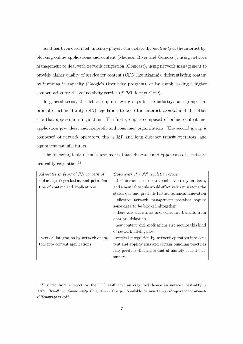
The following table resumes arguments that advocates and opponents of a network
neutrality regulation.12
Advocates in favor of NN concern of Opponents of a NN regulation argue
· blockage, degradation, and prioritiza-
tion of content and applications
· the Internet is not neutral and never truly has been,
and a neutrality rule would effectively set in stone the
status quo and preclude further technical innovation
· effective network management practices require
some data to be blocked altogether
· there are efficiencies and consumer benefits from
data prioritization
· new content and applications also require this kind
of network intelligence
· vertical integration by network opera-
tors into content applications
· vertical integration by network operators into con-
tent and applications and certain bundling practices
may produce efficiencies that ultimately benefit con-
sumers
12Inspired from a report by the FTC staff after an organized debate on network neutrality in
2007: Broadband Connectivity Competition Policy. Available at www.ftc.gov/reports/broadband/
v070000report.pdf.
7

· effects on innovation at the edges of
the network (innovation by content and
applications providers)
· network operators should be allowed to innovate
freely and differentiate their networks as a form of
competition that will lead to enhanced service offer-
ings for content and applications providers and other
end users
· lack of competition in the last-mile
broadband services
· there is insufficient evidence of potential harm to
justify an entirely new regulatory regime, especially
when competition in broadband services is robust
and intensifying and the market is generally charac-
terized by rapid, evolutionary technological change.
· legal and regulatory uncertainty in the
area of Internet access
· prohibiting network operators from charging dif-
ferent prices for prioritized delivery and other types
of quality-of-service assurances will reduce incen-
tives for network investment generally and prevent
networks from recouping their investments from a
broader base of customers, a price which, in turn,
reduce prices for some end users
· diminution of political an other ex-
pression on the Internet.
Table 1: Comparing the arguments for and against regulation.
It is not difficult to notice that the early debate has been carried out in a framework
where the debating parties did not actually convey on what exactly such regulation
would consist of. The truth is that network neutrality means different things to different
people, it depends to who you ask. A modern approach to establish a definition of such
rules would be to consult what industry actors have stated on Wikipedia.13 We can see
that there are different “levels” of network neutrality:
. . . At its simplest, network neutrality is the principle that all Internet traffic should
be treated equally. Net neutrality advocates have established different definitions of
network neutrality:
Absolute non-discrimination Columbia Law School professor Tim Wu: “Net-
work neutrality is best defined as a network design principle. The idea is that
a maximally useful public information network aspires to treat all content,
sites, and platforms equally.”
13See http://en.wikipedia.org/wiki/Network_neutrality
8
Limited discrimination without QoS tiering United States lawmakers have in-
troduced bills that would allow quality of service discrimination as long as no
special fee is charged for higher-quality service.
Limited discrimination and tiering This approach allows higher fees for QoS as
long as there is no exclusivity in service contracts. According to Tim Berners-
Lee: “If I pay to connect to the Net with a given quality of service, and you
pay to connect to the net with the same or higher quality of service, then you
and I can communicate across the net, with that quality of service.” “[We]
each pay to connect to the Net, but no one can pay for exclusive access to me.”
First come first served According to Imprint Magazine, University of Michigan
Law School professor Susan P. Crawford “believes that a neutral Internet must
forward packets on a first-come, first served basis, without regard for quality-
of-service considerations.”
However, what interests us is the economic analysis of network neutrality regulation.
The study of such a regulation from an economics point of view is still progressing. We
can relate the question of network neutrality regulation to issues already studied by clas-
sical economics such as vertical foreclosure, price discrimination, quality differentiation,
two-sided markets pricing, or investment incentives and the hold-up problem.
Economists have divided the analyses of network neutrality regulation into two cat-
egories. First, a regulation that would prohibit ISP from directly charging content
providers for the transmission of their content (like a termination access charge) referred
as the zero-pricing rule. Second, a regulation that would prohibit ISP from propos-
ing different quality of services and prioritizing traffic over their networks, referred as
the non-discrimination rule.14 The introductory section of Chapter 1 details the most
relevant articles so far published by economists.
Chapter 1 of the thesis can be classified within the non-discrimination rule. Bargain-
ing power and the net neutrality debate proposes to study a framework where, as in the
OpenEdge project of Google, a “must-have” content provider would like to enter into
joint investment agreement with two competing ISP in order to increase the quality of its
14This classification was first proposed by F. Schuett (2010), “Network Neutrality: A Survey of the
Economic Literature”, Review of Network Economics, 9(2).
9
online content to, at the same time, raise content consumption and hence its advertising
revenues. A net neutrality regulation would prohibit such vertical agreements.
One of the issues of paramount importance in such configuration is the exclusivity
of content. The Internet has characterized itself so far as an open environment, where
all content is provided to consumers but also where all ISP can provide all the available
content. What would be the effect of such a regulation? On the one hand, prohibiting
vertical agreements would leave the Internet in its actual state where the must-have
content is available to all consumers in equal terms. On the other hand, regulation
would impede investments that would increase the quality of a valuable content but at
the risk of exclusive vertical agreements.
Therefore, the Chapter proposes to examine the effects of the bargaining conditions
between parties in a non regulated environment. In particular, it studies the impact of
the bargaining power of the content provider together with the degree of competition
in the Internet access market over the joint investment agreement or agreements. And
it compares this outcome with the regulated environment outcome where each ISP sets
the quality of the content when they invest by their own means. Investment can be
interpreted as the increase of the capacity of their respective networks.
As it can be noticed in the Table 1 above, investment in networks occupies a central
role in the network neutrality debate. Investment in network infrastructure, in particular
in the next generation access technologies, introduces the second chapter of the thesis.
Next generation access networks
The second Chapter, Investment with commitment contracts: the role of uncertainty,
proposes to explore the incentives to invest in a new network infrastructure when firms
are subject to ex ante access regulation.
As previously discussed in this introduction, the current local loop telephone net-
work, or access network, is an heritage of the formerly monopoly telecommunications
operator. The liberalization process of the telecommunications industry was achieved
10

thanks to regulatory reforms that mandated access, at a regulated price, to the monopoly
infrastructure. Today, the increasing usage of the Internet and the evolution of technical
progress request the upgrade of the old access network. It is expected that next genera-
tion access networks (NGA networks), most likely constituted by fiber-based networks,
replace the inherited copper access network.
European policymakers have announced that it is a priority for the industry to avoid
the establishment of a new monopoly.15 Consequently, policy measures are being taken
to prevent a new infrastructure monopoly. Specific ex ante access obligations will apply
to firms with significant market power over a new infrastructure. Which implies that
firms are certain when taking investment decisions that they will have to open their
network to competitors. As it has been pointed out by economists, ex ante access
obligations clearly discourage investment incentives.
The question is here how to conciliate allocative efficiency (through the promotion of
service competition) and dynamic efficiency (with the creation of investment incentives)
in this new market? As previously discussed, this is not a new question to the sector. In
Europe, policymakers have previously tackled this issue with the theory of the ladder of
investment.16 But in that context the industry counted already with one infrastructure.
The question was rather pointed to the incentives to invest for entrants.
The NGA presents the problem in a somewhat symmetrical perspective: Both the
(now former) entrants and the incumbent have the possibility to invest and deploy a
NGA network.
Another ingredient on top of the static-dynamic tradeoff that seem to be relevant
in this context is firms’ uncertainty about future profits. The retail broadband and
previously dial-up access market developed in the past thanks to the content available
on the Internet. At first, content and applications like web-surfing and e-mailing were the
first drivers of the adoption of dial-up connections. The broadband technology was later
15See the Commission’s Recommendation on regulated access to Next Generation Access Networks.16Although the theory of ladder of investment has been critically questioned, see for example Bour-
reau M., Dogan P., and Manant M. (2010) “A critical review of the ’ladder of investment’ approach”,
Telecommunications Policy, 34.
11

adopted because new applications and content requiring greater bandwidth emerged in
the content market. For instance P2P applications, streaming video, etc. Today the
situation is somehow different. Operators seem to be hesitant about the content drivers
for the migration of users from broadband to super fast broadband Internet access. In
short, there exists incertitude about the profitability of the market.
The objective of the Chapter is then to study incentives of private investment when
firms are subject to ex ante access obligations and when future market profits are uncer-
tain. The Chapter builds a simple game theoretical model of two ex ante symmetric firms
in order to study the effects of a regulated access charge on the market outcome. Before
making investment decisions, the regulator announces the level of the access charge that
the firm without a network will have to pay in order to compete with the one that has
built one.
A central element of the analysis resides on the fact that the profitability of the
market remains unknown until at least one of the firms has decided to incur the sunk
cost of a network. As the rival can always wait for the market profitability to be revealed,
it has naturally incentives to behave in an opportunistic way before incurring the sunk
cost itself.
The Chapter aims at proving that richer forms of access contracts between firms can
attenuate the opportunistic behavior and increase investment incentives. In particular,
access contracts with commitment clauses between firms where one firm commits to buy
access from the other one independently of the market profitability better allocate the
risk of investment between both firms.
As it will be developed throughout the Chapter, the industrial organization literature
on the impact of access regulation on broadband investment takes three approaches.
Fist, a body of literature focuses on asymmetric frameworks where an entrant who
enjoys regulated access to the incumbent’s network invest and builds its own network.
A second body of literature studies the incentives of an incumbent to upgrade its network
when subject to mandated access. And finally, the third body of literature, closer to
12

this Chapter, focuses on a more symmetric situation where both the former incumbent
and entrant must build the network from “scratch”. In this literature, inspired from the
patent race work, the role of the incumbent is endogenous. The object of study is then
to determine the investment date when firms know that the sunk cost of the network
deployment decreases in time as a result of technological progress.
As in the patent rase literature, cost reduction is the outcome of an technological
progress that is exogenous to the model. But actually, and in particular for the telecom-
munications industry, the progress of technology is rather an endogenous process. Firms
reinvest their profits in R&D in order to lower their costs. This is the motivation that
leads us to the third Chapter of the dissertation.
Technological progress
The objective of the third Chapter is to revisit the link between competition and inno-
vation in a rather original framework. Two elements motivate a revisit of this classic
question.
The first element comes from personal amazement. One can effortlessly observe the
constant technological progress in the information technology industry and in particular
in the telecommunications sector. A recent study has collected 100 and plus years of
data to measure and compare the technological progress in these industries.17 The study
quantifies our observation: the annual progress rate ranges from 20% to 40%!
One can conclude that if studied from a long term point of view, it is pertinent to
consider technological progress and innovation as an incremental process rather than a
disruptive process as typically addressed by the patent literature.
The second element comes from the particularity of regulated sectors. In many mar-
kets and specifically in the mobile telephony market, entry is limited by a social planner.
By limiting access to an activity, the social planner has the ability to artificially create
17See Koh and Magee (2006), “A functional approach for studying technological progress: Application
to information technology”, Technological Forecasting & Social Change, 73(9).
13

scarcity which increases market prices. By the same mechanism, a social planner can in-
crease the number of firms in the market and induce a reduction of prices redistributing
resources from firms to consumers. We have repeatedly learnt that perfect competition is
the optimal market performance. But this is true only in situations where technological
advance is unaffected by resource allocation.
It is then important for a social planner to consider which is the optimal level of
competition that maximizes welfare in an industry where technological progress is en-
dogenous and incremental.
The question of market structure and investment has been long treated by economists
going back to Schumpeter and Arrow. Economics literature on the subject is more
polemic than consensual. Empirical economists make the distinction among two different
questions: the impact of market structure on innovational effort and on innovative
results.18 The Chapter and our interest focuses on the former question accepting that
greater efforts lead to more innovative results.
Early empirical literature examining the impact of market concentration on research
effort has found varying results and little consensus.19 A share of the literature finds
that firms in concentrated industries spend more on research activities whereas exactly
another portion find insignificant and even a negative relationship. The variation of
results can be attributed to diverse factors. This might be because the empirical tests
where realized in different countries, but also there exist deficiencies on the proxies for
calculating innovational efforts.20 A further caveat of empirical studies resides on the
fact that standard measures of market concentration quantify only current active firms
in the market, hence it might omit potential rivalry and dynamic strategy motives.
18It has been observed that smaller firms have more flexible organizational structures which makes
them more dynamic and efficient when transforming innovative effort into innovative results.19For a detailed review of the literature see Kamien M. I., and Schwartz N. L. (1975), “Market Structure
and Innovation: A Survey”, Journal of Economic Literature, 13(1).20Usual measures of innovative effort include R&D spending or scientific employees, yet technological
improvements are not always made in R&D departments. Further, this measures can be affected by
institutional bias. For example, if public policies cut taxes for R&D spending firms might have incentives
to blow research spendings out of proportion.
14

More recently,21 economists have found that the relationship between competition
and innovation is not linear. By plotting a weighted measure of patents against the
Lerner index they conclude that an inverted-U best suits the relationship. That is,
mildly concentrated industries innovate more. If more innovation implies higher welfare,
one can agree that moderately concentrated markets are preferable.
On the theoretical approach the literature has mostly concentrated, as mentioned,
on the questions of disruptive innovative process. The originality of this Chapter is then
to study this question using game theoretical tools that allow for the explicit account of
the incremental nature of technological progress.
The Chapter builds a differential game where n firms invest profits gained today in
order to reduce costs incurred tomorrow. The number of firms active in the market
is, as in the mobile telephony sector, set by a social planner. As the recent empirical
literature, the Chapter highlights the role of imperfect competition in innovation. The
differential games approach allows for a clear study of the dynamic effects of competition
(investment) versus the static effects (allocation of resources).
Each chapter of the dissertation is self-contained. In order to facilitate its read-
ing, mathematical demonstrations have been arranged in appendices at the end of each
chapter.
21A well know recent reference is Aghion et al (2005), “Competition and Innovation: An Inverted-U
Relationship”, Quarterly Journal of Economics, 120(2).
15

16

Chapter 1
Bargaining power and the net
neutrality debate
1.1 Introduction
The Internet was conceived more than 30 years ago to treat all data traffic equally, in
a neutral way. During these last years this neutrality principle has been challenged at
several levels which has led to a debate on whether this original neutrality principle of
the Internet should be preserved.
The resulting ongoing debate, referred as network neutrality, encompasses the possi-
bility of regulating the Internet in order to maintain the neutrality principle. Different
degrees of regulation have been proposed in order to either penalize content blocking,
to avoid further content providers taxation by network operators or even to prevent
quality of service agreements. The debate clearly opposes two groups in the industry:
the side that promotes a regulation regrouping online content and application providers
with nonprofit and consumer organizations against network operators and equipment
manufacturers who oppose it. In short, the former argue that letting operators have
control over online content would distort the Internet content market. The latter op-
pose to regulation claiming that the Internet has proven to be competitive and that
further gains on content quality of service improvement and network investment could
be attained without regulatory constraints.
17

As this paper is written there is formally no regulation that forbids access providers
from offering quality enhancement contracts. Competition authorities have stated that
blocking online content will not be allowed except for reasonable network management
and accordingly all content blocking has been penalized ex post. But all attempts to
pass legislation in the US have so far failed.1 In Europe there is no specific legislation
on net neutrality, quality differentiation provision is theoretically allowed as long as this
does not lead to anticompetitive effects. The possibility of offering priority services is
still open as well as efforts to regulate the market.
The economics literature on network neutrality has focused so far on different and
scattered issues. This is probably due to the complexity of the ongoing debate. At
this stage, net neutrality means different things to different people. Nonetheless several
aspects of the debate find their parallel with more classic economics literature.2 These
include vertical foreclosure, price discrimination, quality differentiation, two-sided mar-
ket pricing, investments incentives and the hold-up problem.
Hermalin and Katz (2007) apply the theory of product-line restriction to the net
neutrality debate. They consider an access provider that brings together consumers and
a continuum of content providers. Under an unregulated regime, the platform can sell
different levels of quality to content providers, opposed to a net neutrality regime, where
the platform chooses a unique quality level for all content. They find that with net
neutrality the platform sets a quality service that gives rise to three effects: low-value
content providers, who would had otherwise bought low quality from the platform, are
excluded from the market; mid-value content buy higher quality services; and high-value
content buys lower quality. Net welfare effects of net neutrality are likely to be negative.
Moreover, net neutrality would harm low-value or small content providers rather than
protect them, leaving consumers with fewer content which opposes the objective of the
regulation proponents.
Economides and Tag (2007) take a two-sided market pricing approach and they
1For example Bill numbers H.R. 5252, H.R. 5417, S. 2686, etc.2For a global analysis refer to Kocsis and de Bijl (2007).
18

suppose, unlike Hermalin and Katz, that all content is homogeneous. They compare
welfare in the case where the platform can charge content providers with the regulated
net neutrality regime where the platform can only charge consumers. They find, contrary
to Hermalin and Katz (2007), that welfare increases with regulation. If content providers
are charged, the two-sided pricing mechanism lowers consumers’ access prices but reduces
the available content providers in the market, which reduces overall welfare.
Choi and Kim (2010)3 analyze the impact of vertical quality of service agreements on
investment incentives. They consider an Internet access provider who has the ability to
offer priority transmission in a congested network to two competing content providers.
In a net neutrality regime both content providers receive the same treatment and hence
compete for consumers in equal terms whereas in the unregulated regime the traffic of
one content provider is favored over the traffic of the other one. In this framework, they
find that content providers face a prisoners’ dilemma to pay for priority and they are
worse-off without net neutrality. The Internet access provider faces a trade-off, either it
invests in expanding its capacity to have a larger revenue from consumers or it maintains
scarcity in order to charge content providers for priority. Overall welfare implications
are not clearcut, however they show that network investment incentives could be higher
under net neutrality, which contradicts the arguments of the opponents of a regulation.
On the other hand, investment implications are clear for content providers, the authors
affirm that these are undoubtedly reduced under the unregulated regime because the
network operator has the power to expropriate content providers’ rents.
In general terms, the net neutrality debate has been often perceived as a trade-off
between innovation at the edges of the Internet (innovation of content providers) and
investment within the Internet (infrastructure investments). But profits, and therefore
incentives to innovate and invest, of content and access providers are not necessarily
opposing. With a better quality of service online content is improved and generates
two sources of revenue, it increments advertising revenues and consumers’ willingness to
3The forthcoming article of Cheng et al. (2011) study a similar model obtaining similar results.
19

pay for Internet access. Hence, there might exist a mutual benefit to invest if contracts
between content and access providers are agreed before investment, avoiding the hold-up
problem encountered by Choi and Kim (2010).
Adding to the existing literature, this paper considers a scenario where a content
provider negotiates with two competing Internet access providers for an investment con-
tract to improve the existing quality of service. It complements the existing literature
as it focuses on the effects of departing from net neutrality in a context where the bar-
gaining power is no longer concentrated on the Internet access providers’ side. This
approach is relevant as we observe an increasing concentration in some sectors of the
online content provision.4
The net neutrality regime is understood as a situation where network operators and
the content provider cannot enter in any form of quality agreement. In this regime
the network operators invest on the quality of service by their own means. Whereas
in the second one, the unregulated regime, the content provider can participate in the
investment process by negotiating quality contracts with one, both or none of the network
operators. The paper focuses on the effects the content provider’s bargaining power has
on the quality of service agreements, comparing investments outcomes in each regime.
To this end, two specific features of the Internet are taken into account. First it
is supposed that global connectivity on the Internet allows consumers to have access to
the content even if the content provider does not have an agreement with their net-
work operator. And second, Internet access providers have control over the last-mile, or
the bottleneck to consumers, which allows them to unilaterally control the consumers
perceived quality of the content.
Not surprisingly, allowing contractual relations between content and access providers
yields higher investment on quality. Improved quality of content results in more content
consumption, bringing higher advertising revenues that are used to cover investment
4This is turn has led to heterogenous interconnection agreements between content providers and
network operators, favoring big providers, see for example http://www.wired.com/epicenter/2009/10/
youtube-bandwidth/.
20

costs. At the same time an unregulated regime might as well lead to adverse effects.
If a network operator is excluded from the negotiation process while the other network
operator reaches an agreement with the content provider, the excluded operator has
incentives to degrade the quality of the content. In effect, the excluded operator does
not count with the financial support of the content provider whereas its competitor does
which allows him to set a quality superior to the one with independent investment. The
quality difference shifts the demand for Internet access towards the operator providing
the high-quality content. Hence, facing this disadvantage and anticipating lower retail
revenues the excluded operator prefers to degrade the quality of content given that
quality is costly.
The ability of access providers to lower content’s quality of service has consequential
strategic implications for the content provider when deciding whether to enter into joint
investment agreements. The content provider can either have an agreement with both
network operators and raise its quality for all consumers, or he can enter into an exclusive
quality deal with one operator. With exclusivity the content provider faces a trade-off.
On the one hand it receives fewer adverting revenues because consumers accessing the
content through the excluded operator perceive a degraded quality. On the other hand,
the content provider would pay less for the quality given that: first it invests with one
operator only and second because the operator with the exclusive deal is willing to
accept a smaller financial contribution for the increased quality as exclusivity gives him
an advantage on the access market.
A content provider with bargaining power has the ability to negotiate a contract that
allows him to keep most of the advertising profit, he then chooses to enter into a simulta-
neous quality agreement with both access providers. Whereas a small content provider
gets his rents extracted during negotiation, he will then use the exclusive agreement as
a leverage to increase his position in the negotiation process.
Additionally, the model takes into account the role of competition intensity on the
access market. When access competition is not too strong an access provider is less
21

concerned about the quality offered by its competitor. Then, the degradation of content
is less severe. With strong competition in the access market the content degradation is
aggravated which exacerbates the vulnerability of weak content providers.
Finally, the model finds that consumer welfare is higher when access and content
providers are free to negotiate. This result also holds when the content provider decides
to enter into exclusive agreements.
The rest of the paper is organized as follows: section 2 presents the framework of
the model, section 3 develops the net neutrality benchmark. The non regulated regime
is analyzed in section 4, where simultaneous or exclusive quality enhancement contracts
between content and access providers can be negotiated. Section 5 discusses competition
policy implications, to continue with some extension in section 6 and to finally conclude
in section 7. All technical proofs can be found in the appendix.
1.2 The Model
Consider two Internet service providers, denoted by ISP1 and ISP2, that compete for
consumers who want to have access to a specific Internet content, online service or
application offered by a content provider denoted by CP. Consumers pay only for the
Internet access service and not for content consumption, content provider’s revenues
come from online advertising.
Two important and specific features of the Internet are taken in consideration in this
model:
Global connectivity The Internet is a global network. A service provider ISPi can
offer the content of CP even if ISPi has no direct interconnection or contract rela-
tion with CP. And vice-versa, the CP receives online advertising revenues without
directly remunerating access providers for the connection provided to consumers.
Last-mile control Access providers control what is known as the last mile. Because
access providers manage the last segment of the path that connects CP to con-
22

sumers, they have control over the final transmission quality of the content.
It will be later evident how these two features characterize the hypothesis of the model,
demand and costs structures are now described.
Demand structure There is a continuum of consumers of the same type. All con-
sumers use both ISP1 and ISP2 to have access to CP.5 The representative consumer
that consumes qi units of content using access of ISPi, i ∈ 1, 2, has a quadratic utility
u(q1, q2) = α1q1 + α2q2 − 12(q21 + 2γq1q2 + q22), where αi is the quality of service that
access providers set in the last mile for the CP. The parameter γ ∈ [0, 1) represents the
differentiation between access providers.6 With γ close to 0, a consumer using access of
ISPi does not reduce his utility from using access of ISPj to get the content. This would
be the case of mobile access vs. fixed line access for someone that travels as much as
stays at home. On the other hand, with γ close to 1 access providers are perfect sub-
stitutes. This could be illustrated by someone having cable and ADSL access at home.
As it is frequent in the economic literature, the parameter γ can be reinterpreted as a
proxy of competition intensity on the Internet access market.
Given pi the access price set by the access provider ISPi, the representative consumer
maximizes his net utility maxq1,q2 u(q1, q2) − p1q1 − p2q2. This utility function gives
rise to a linear demand structure, inverse demands are given by pi = αi − qi + γqj . The
linear demand for access provider ISPi is given by
qi = q ((αi, pi), (αj , pj)) ≡1
1 − γ2(αi − pi − γ(αj − pj)) .
Cost structure In order to set the quality of service α, an access provider must make
an investment of I(α). Last-mile quality upgrade investments in telecommunications are
known to be very costly.7 The model supposes that this investment is fixed and it does
5Section 6 shows that most results are robust in a context where consumers are horizontally differ-
entiated and choose one access provider only.6We have come to a state where Internet access technologies can take the form of dial-up, landline
(over coaxial cable, fiber optic or copper wires), T- lines, Wi-Fi, satellite and cell phones.7See Faulhaber and Hogendorn (2000) or Fijnvandraat and Bouwman (2006).
23

not depend on variable content consumption. It further supposes that access providers
have the basic infrastructure to provide a minimal quality, so the marginal increase for
low qualities of service is small compared to a marginal increase for higher qualities.
Technically I(·) is set to be an increasing differentiable “very” convex function, with
I ′(·) a convex function as well,8 and with I(0) = I ′(0) = 0. For expositional clarity
purposes let us fix the investment cost function to I(α) = α3
6 . But no specification of
the investment function is necessary to show general results. For the sake of simplicity,
other costs and marginal costs are normalized to zero.
Access provider ISPi’s profit from access consumption is
πi = piqi − I(αi)
Content provider Revenues for the content provider come from advertising and they
are increasing with content consumption. An increase of quality increases content con-
sumption. For simplicity the model supposes that publicity revenues net of operation
costs are linear. The content provider has advertising profits
πc = q1 + q2.
The game Two different regulatory regimes will be studied. In the first regime, that
will be called the net neutrality regime, the content and access providers are not allowed
to enter into any form of agreement. In the second unregulated regime, the content
provider can participate in the investment process that determines his quality of service.
In general terms and depending on the regime, the timing9 of the game is as follows:
First there is an investment stage where the quality of service αi, αj is fixed according
to the regulatory regime; and second the access competition stage where access providers
set subscription prices pi, pj for consumers non-cooperatively. The timing is chosen
8Other authors that use convex marginal costs for quality in different contexts are Schlee (1996) and
Johnson and Myatt (2003)9Details of each stage will be specified further on section 1.4.
24

to reflect the versatility of price setting after an infrastructure investment, characteris-
tic of the telecommunications sector, which is standard in the economics literature on
investment.
1.3 The benchmark: Net neutrality
In this section we set as benchmark the net neutrality regime where the content provider
does not participate on the investment process. The timing of the game is as follows
(1) Investment, quality of service levels αi, αj are set by access providers non-
cooperatively
(2) Access competition, access prices pi, pj are fixed by access providers non-cooperatively
In this regime, the content provider plays a passive role in the game. There is no
relation between the network operators and the content provider, there are no fees for
content access nor fees for network usage, and all decisions are made by access providers
only. However the content still generates advertising profits as a consequence of global
connectivity.
Access competition The solution concept is sub-game perfect Nash equilibria. Given
qualities αi, αj set at stage (1), provider ISPi sets at stage (2) his price pi, taking pj
as given, to maximize his profits
maxpi
πi = pi1
1 − γ2(αi − pi − γ(αj − pj)) − I(αi)
The first order condition gives rise to the following reaction function Rpi (pj) = 12(αi −
γ(αj − pj)). Notice that when γ is small ISPi can price consumers proportionally to the
quality he sets, but when γ increases price competition in the access market intensifies
and prices adjust to the rival’s offer. Solving the system of reaction functions there exists
a unique price equilibrium given by:
p∗i = p(αi, αj) ≡1 − γ
2 − γαi +
γ
4 − γ2(αi − αj) (1.1)
25
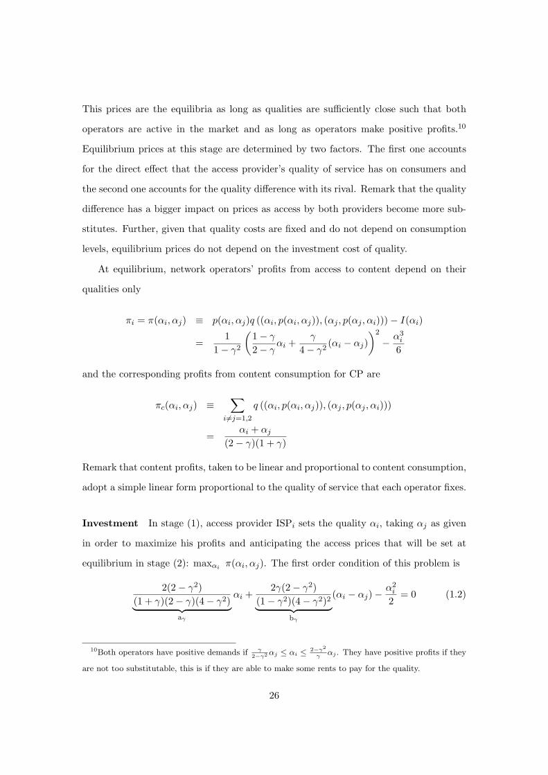
This prices are the equilibria as long as qualities are sufficiently close such that both
operators are active in the market and as long as operators make positive profits.10
Equilibrium prices at this stage are determined by two factors. The first one accounts
for the direct effect that the access provider’s quality of service has on consumers and
the second one accounts for the quality difference with its rival. Remark that the quality
difference has a bigger impact on prices as access by both providers become more sub-
stitutes. Further, given that quality costs are fixed and do not depend on consumption
levels, equilibrium prices do not depend on the investment cost of quality.
At equilibrium, network operators’ profits from access to content depend on their
qualities only
πi = π(αi, αj) ≡ p(αi, αj)q ((αi, p(αi, αj)), (αj , p(αj , αi))) − I(αi)
=1
1 − γ2
(1 − γ
2 − γαi +
γ
4 − γ2(αi − αj)
)2
− α3i
6
and the corresponding profits from content consumption for CP are
πc(αi, αj) ≡∑
i6=j=1,2
q ((αi, p(αi, αj)), (αj , p(αj , αi)))
=αi + αj
(2 − γ)(1 + γ)
Remark that content profits, taken to be linear and proportional to content consumption,
adopt a simple linear form proportional to the quality of service that each operator fixes.
Investment In stage (1), access provider ISPi sets the quality αi, taking αj as given
in order to maximize his profits and anticipating the access prices that will be set at
equilibrium in stage (2): maxαiπ(αi, αj). The first order condition of this problem is
2(2 − γ2)
(1 + γ)(2 − γ)(4 − γ2)︸ ︷︷ ︸
aγ
αi +2γ(2 − γ2)
(1 − γ2)(4 − γ2)2︸ ︷︷ ︸
bγ
(αi − αj) −α2i
2= 0 (1.2)
10Both operators have positive demands if γ
2−γ2 αj ≤ αi ≤2−γ2
γαj . They have positive profits if they
are not too substitutable, this is if they are able to make some rents to pay for the quality.
26

Here, aγ = 2(2−γ2)(1+γ)(2−γ)(4−γ2)
is the marginal revenue gain that an access provider makes
from a quality of service increase, independent of what the other access provider sets as
quality. It can be easily verified that the parameter aγ is positive and that it strictly
decreases with the substitution parameter. The other parameter bγ = 2γ(2−γ2)(1−γ2)(4−γ2)2
is
the marginal revenue gain (or loss) that an access provider makes from offering a higher
(or lower) quality of service compared to its rival. With two independent access providers
b0 = 0, but more substitutable operators face more frontal competition as bγ increases.
The best reply function for access provider ISPi is
Rαi (αj) =
aγ + bγ +√
(aγ + bγ)2 − 2bγαj , if αj ≤ (aγ+bγ)2
2bγ
0, otherwise
Observe that the reply function is strictly decreasing with the competitors quality. If
ISPj increases his quality, the access provider ISPi anticipates that in the access pricing
stage he will have to reduce his access prices at equilibrium, and having less access rev-
enues ISPi has no option other than to decrease the quality of service proposed given the
high investment costs. With αj high enough, ISPj could foreclose ISPi from the market.
Technically this corresponds to the situation where ISPi has strictly decreasing profits
for any set of quality levels.
There exists a symmetric solution of the system (1.2) above, or equivalently a fixed
point for the best replies system αn = Rαi (αn) given by
αn = 2aγ
This is the equilibria as long as the second order condition holds: aγ+bγ < I ′′(αn) = 2aγ .
Equivalently, this condition holds if marginal revenues from direct consumption exceed
marginal revenues from quality competition with the rival: aγ > bγ which holds for
γ < γn =√
3 − 1. If γ > γn the profit is not concave, this comes from the fact that
quality costs are fixed and do not depend on the quality. However the range of parameters
for which equilibria exists can be extended by setting a “more convex” investment cost.
The following proposition resumes the exposed above.
27

Proposition 1.1. If access providers are not too substitutable γ < γn, then there exists a
sub-game perfect Nash equilibria which is symmetric where Internet access providers set
a quality equal to αn. The quality decreases as access providers become closer substitutes.
Proof. All details of technical proofs are found in the appendix.
There exists as well an asymmetric equilibrium where one operator invests more
than the other. However this equilibrium exits for a small range of substitutability
between access providers. This equilibrium is not really important in the analysis because
total symmetry between access providers suggest that a symmetric equilibrium is more
relevant. The interested reader may consult the appendix.
This sets the benchmark for the second regime where CP can participate in the
investment process by negotiating a quality enhance with the access providers ISPi. In
what follows, the non regulated regime is analyzed.
1.4 No Regulation
With no regulation, the content provider can participate on the investment process. The
investment stage of the game is subdivided in two periods
(1) Investment. The content provider CP proposes to negotiate an investment agree-
ment over the terms of a quality level αi and a fixed monetary transfer Ti to
either:
- Both access providers, having simultaneous contracts
- One access provider only, where CP enters into a quality exclusive agreement
- None of them, and access providers invest by their own means, as in the net
neutrality regime
(2) Access competition. access prices pi, pj for consumers are fixed non-cooperatively
by ISPi and ISPj .
28

Given that the transfer fee T negotiated in stage (1.2) is fixed, it does not impact
prices set by access providers in stage (2). So the access price equilibrium is the same
as in the net neutrality regime, as in equation (1.1). Total profits for the providers are
profits from content access or advertising at the agreed quality levels plus or minus the
agreed monetary transfer:
Πi = Π(αi, αj ;Ti) ≡ π(αi, αj) + Ti, Πc(αi, αj ;Ti, Tj) ≡ πc(αi, αj) − Ti − Tj
If there is no agreement Ti = 0 and the quality αi is set unilaterally by the access
provider.
The outcome of the negotiation process between the content provider and access
providers is taken to be the Nash equilibrium of simultaneous generalized Nash bargain-
ing problems.
1.4.1 Simultaneous contracts
Suppose that CP has decided to negotiate with both access providers, and that both
access providers decide to enter into negotiation.
Bargaining framework There are four assumptions that determine the solution of
the bargaining process. First, as it is usual in the literature of vertical relations for its
tractability, the model supposes that negotiations between the pair CP , ISP1 and
the pair CP , ISP2 occur simultaneously.11 The equilibrium concept that is used is
somehow close to the contract equilibrium first formalized by Cremer and Riordan (1987).
This means that at equilibrium, the contract agreed by the pair CP , ISPi must be
immune to unilateral deviations. Second, the solution supposes that contracts negotiated
are not contingent on rival pair’s disagreement.12 This means that the bargaining pair
11See for example Horn and Wolinsky (1988); O’Brien and Shaffer (1992); Milliou and Petrakis (2007);
Allain and Chambolle (2007).12Examples of authors that use this hypothesis are Horn and Wolinsky (1988); O’Brien and Shaffer
(1992); McAfee and Schwartz (1994).
29

CP , ISPi cannot implement a contract that specifies another outcome if the bargaining
process of the other pair CP , ISPj has failed. Third, as a consequence of the last-mile
control property, the model supposes that the outside option αi for the access provider
ISPi is a best response to the other pair’s agreed quality αj . This assumption implies
that the equilibrium outcome is sub-game perfect. And finally, the model supposes that
access providers are completely symmetric, this means that the content provider has the
same exogenous bargaining power β ∈ (0, 1) with respect to each one of them.
Having this said, the program that the pair CP , ISPi solves in this simultaneous
setting taking the rival pair’s contract α∗j , T
∗j as given is
maxαi,Ti
Π(αi, α
∗j ;Ti) − Π(αi, α
∗j ; 0)
1−β Πc(αi, α
∗j ;Ti, T
∗j ) − Πc(αi, α
∗j ; 0, T
∗j )β
(1.3)
where outside option quality is
αi = arg maxα
π(α, α∗j ) (1.4)
The monetary transfer that maximizes (1.3) is easily calculated
T ∗i = (1 − β)
(πc(αi, α
∗j ) − πc(αi, α
∗j ))− β
(π(αi, α
∗j ) − π(αi, α
∗j ))
Note that the transfer fee T ∗i does not depend on the other pair’s monetary transfer.
Actually, one can make the parallel of this model with classical vertical relations lit-
erature where the producer charges two-part tariffs to distributors. Here the quality
level occupies the role of the linear part of the tariff which is usually set to maximize
the bargaining pair’s joint profits. The fixed part, here the transfer fee, distributes the
surplus according to their respective bargaining power. Then, by plugging T ∗i into the
program (1.3), we find that it can be easily reduced to
maxαi
(πc(αi, α
∗j ) − πc(αi, α
∗j ))
+(π(αi, α
∗j ) − π(αi, α
∗j ))
(1.5)
The first order condition for this problem is
2(2 − γ2)
(1 + γ)(2 − γ)(4 − γ2)︸ ︷︷ ︸
aγ
αi+2γ(2 − γ2)
(1 − γ2)(4 − γ2)2︸ ︷︷ ︸
bγ
(αi−αj)+1
(2 − γ)(1 + γ)︸ ︷︷ ︸
cγ
−α2i
2= 0 (1.6)
30

where aγ and bγ are as in equation (1.2), and cγ = 1(2−γ)(1+γ) is the marginal revenue
the content operator gets with an augmentation of the quality αi.
The solution of the system above has a symmetric equilibrium given by
αs = aγ +√
aγ2 + 2cγ
Clearly αs > αn as long as cγ > 0, the quality set with simultaneous contracts is
higher than the one set in a net neutral regime if the content provider makes profits
with a quality increase. However again, this result holds when the operators are not
too substitutable. Equilibria might fail to exist as in the previous regime when bγ <√
aγ2 + 2cγ , or equivalently for γ < γs ≈ 0.89.
The outside option In a simultaneous setting, the outside option quality αs is the
quality that access provider ISPi would set if no agreement is reached with CP and if
the other pair CP , ISPj holds to the equilibrium quality αs. The access provider
ISPi then solves the program (1.4), it maximizes its revenues maxαiπi(αi, αs). Then αs
equals
αs = aγ + bγ +√
aγ2 + bγ2 − 2bγ
√aγ + 2cγ
When access providers enjoy a local monopoly positions and γ = 0, b0 = 0 and the
outside option is the same quality as in the net neutral regime. However, if γ > 0,
ISPi anticipates that the other pair’s higher quality forces him to set lower prices, and
hence lower revenues. As a result ISPi sets a quality lower that the quality set under
net neutrality. As discussed in section 1.3, Rαi decreases with αj , then αs = Rαi (αs) <
Rαi (αn) = αn. In a Nash bargaining setting, the outside option is frequently interpreted
as a threat point. Notice that in this case, to set a quality lower than the one in a net
neutrality regime is a threat that is credible, given that the access provider maximizes
his revenues.
Letting access providers have control over the outside option is a characteristic of
this model that distinguishes it from traditional vertical relationships. In a producer-
distributor relation, in case of no agreement the producer does not provide the product
31
to the distributor, so the outside option profit for the distributors is zero as he has no
product to retail. Here, the access providers as distributors of content do have power
over the last segment of the network. As the Internet offers global connectivity the
content is available to the Internet access provider always.
The discussion above is summarized in the following proposition:
Proposition 1.2. Suppose that the content provider CP selects to enter into simulta-
neous negotiations with both access providers.
- If access providers are not too substitutable γ < γs there exists a symmetric contract
equilibria where the quality is αs.
- The quality set when a simultaneous contract is established is greater than the
one set in a net neutrality regime, αs > αn, however the quality set by an access
provider in case of no agreement with the content provider is lower than the net
neutrality one αs ≤ αn.
As αs maximizes ISPi’s profit πi(αs, αs) < πi(αs, αs). This implies that the transfer
fee is always from the content provider to the access provider, i.e. CP helps to pay for
the quality augmentation costs. The transfer fee is
TS = (1 − β)∆Sc − β∆S
where ∆Sc = πc(αs, αs) − πc(αs, αs) ≥ 0 is the value for CP of a successful negotiation
with one access provider in the simultaneous bargaining setting, and ∆S = π(αs, αs) −
π(αs, αs) ≤ 0 is the minimal compensation an access provider is willing to accept in
order to invest αs. Total profits are
Πsi = π(αs, αs) + TS (1.7)
Πsc = πc(αs, αs) − 2TS
1.4.2 Exclusive contracts
Suppose now that CP has decided to negotiate with only one access provider, lets say
ISPi, who accepts to negotiate with him leaving aside the access provider ISPj . As in
32
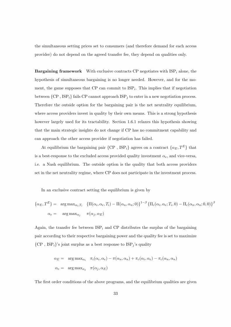
the simultaneous setting prices set to consumers (and therefore demand for each access
provider) do not depend on the agreed transfer fee, they depend on qualities only.
Bargaining framework With exclusive contracts CP negotiates with ISPi alone, the
hypothesis of simultaneous bargaining is no longer needed. However, and for the mo-
ment, the game supposes that CP can commit to ISPi. This implies that if negotiation
between CP , ISPi fails CP cannot approach ISPj to enter in a new negotiation process.
Therefore the outside option for the bargaining pair is the net neutrality equilibrium,
where access providers invest in quality by their own means. This is a strong hypothesis
however largely used for its tractability. Section 1.6.1 relaxes this hypothesis showing
that the main strategic insights do not change if CP has no commitment capability and
can approach the other access provider if negotiation has failed.
At equilibrium the bargaining pair CP , ISPi agrees on a contract αE , TE that
is a best-response to the excluded access provided quality investment αe, and vice-versa,
i.e. a Nash equilibrium. The outside option is the quality that both access providers
set in the net neutrality regime, where CP does not participate in the investment process.
In an exclusive contract setting the equilibrium is given by
αE , TE = arg maxαi,TiΠ(αi, αe, Ti) − Π(αn, αn; 0)1−β Πc(αi, αe;Ti, 0) − Πc(αn, αn; 0, 0)β
αe = arg maxαjπ(αj , αE)
Again, the transfer fee between ISPi and CP distributes the surplus of the bargaining
pair according to their respective bargaining power and the quality fee is set to maximize
CP , ISPi’s joint surplus as a best response to ISPj ’s quality
αE = arg maxαiπi(αi, αe) − π(αn, αn) + πc(αi, αe) − πc(αn, αn)
αe = arg maxαjπ(αj , αE)
The first order conditions of the above programs, and the equilibrium qualities are given
33
by the system
aγαE + bγ(αE − αe) + cγ =α2E
2(1.8)
aγαe − bγ(αE − αe) =α2e
2(1.9)
The explicit solution of this system is cumbersome, however there are important prop-
erties that can be deduced. In an access market where providers are completely in-
dependent γ = 0 equation (1.8) coincides with equation (1.6), the quality set by the
access provider with the exclusive deal equals the one in a simultaneous contract setting
αE = αs. Additionally, as equation (1.9) coincides with equation (1.2), the quality set
by the excluded access provider is the same as in a net neutral regime αe = αn. With
γ > 0 the term accompanied by bγ > 0 gains importance and the bargaining pair gets
more revenues from the quality difference. The content provider can further commit to
ISPi setting an even higher quality αE > αs than in the simultaneous contract setting.
As access providers become more substitutable it is easier to capture rival’s demand
by increasing quality. The best response for the excluded operator is to set a quality
αe < αn lower than in the net neutrality regime.
Foreclosed market The difference in qualities grows up to a point where the excluded
access provider lowers his quality until his revenues are so small that he cannot cover
quality costs and he is foreclosed from the market. This corresponds to the limit situation
where the pair CP , ISPi set a quality for which Rαj (αE) = 0 and this quality is
the best for the bargaining pair. Beyond this threshold the pair CP , ISPi sets a
quality corresponding to a monopoly access, or equivalently to the quality set for γ = 0,
αM = a0 +√
a20 + 2c0.
Even if foreclosure equilibria might arise, the focus of the paper will be on the shared
market equilibria. From now on suppose that access providers are not too close substi-
tutes, or otherwise put, that competition between access providers is not too strong. It
can be agreed that this assumption fits well the Internet access market, as it is generally
an oligopolistic market. The proposition follows
34

Proposition 1.3. Suppose that the content provider CP selects to negotiate only with
access provider ISPi. There exists a threshold γe such that,
- If γ < γe, there exists an equilibrium αE , αe where both access providers are
active in the access market. The excluded access provider, ISPj, offers the content
with a lower quality αe < αE.
- The equilibrium qualities satisfy αe ≤ αs ≤ αn < αs ≤ αE
- Beyond the threshold the bargaining pair sets quality at the monopoly level excluding
ISPj from the access market.
With exclusive contracts one part of the population has access to the content with
high quality and the other part with low quality. When comparing the average qualitie
we have the following corollary.
Corollary 1.1. The average quality with exclusive contracts is higher than the quality
with net neutrality but lower than the quality with simultaneous contracts. This is
αn <αE + αe
2< αs (1.10)
Figure 1.1 bellow illustrates the equilibrium qualities for each regime.
Γ
ΑE
Αs
Αn
ΑsΑe
marketforeclosure
.γe
Figure 1.1: Equilibrium qualities for different regimes and different contract choices
The monetary transfer is
TE = (1 − β)∆Ec − β∆E
35
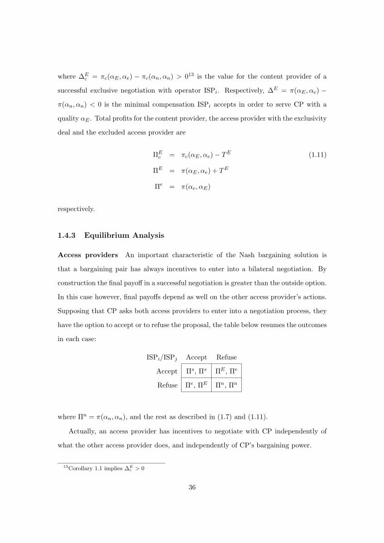
where ∆Ec = πc(αE , αe) − πc(αn, αn) > 013 is the value for the content provider of a
successful exclusive negotiation with operator ISPi. Respectively, ∆E = π(αE , αe) −
π(αn, αn) < 0 is the minimal compensation ISPi accepts in order to serve CP with a
quality αE . Total profits for the content provider, the access provider with the exclusivity
deal and the excluded access provider are
ΠEc = πc(αE , αe) − TE (1.11)
ΠE = π(αE , αe) + TE
Πe = π(αe, αE)
respectively.
1.4.3 Equilibrium Analysis
Access providers An important characteristic of the Nash bargaining solution is
that a bargaining pair has always incentives to enter into a bilateral negotiation. By
construction the final payoff in a successful negotiation is greater than the outside option.
In this case however, final payoffs depend as well on the other access provider’s actions.
Supposing that CP asks both access providers to enter into a negotiation process, they
have the option to accept or to refuse the proposal, the table below resumes the outcomes
in each case:
ISPi/ISPj Accept Refuse
Accept Πs, Πs ΠE , Πe
Refuse Πe, ΠE Πn, Πn
where Πn = π(αn, αn), and the rest as described in (1.7) and (1.11).
Actually, an access provider has incentives to negotiate with CP independently of
what the other access provider does, and independently of CP’s bargaining power.
13Corollary 1.1 implies ∆Ec > 0
36

Proposition 1.4. Negotiate with the content is a dominant strategy for access providers.
Moreover, when the content is powerful, access providers face a prisoners dilemma.
Content provider For the content provider the situation is different. As he antici-
pates that access providers accept to negotiate with him, he has the final choice on the
equilibrium outcome.
The following lemma will be of use, after giving some insights of its consequences the
following paragraph analyzes content provider’s contract choice.
Lemma 1.1. Suppose that access providers are not too substitutable, then
(i) The value for CP of a successful negotiation with one network operator is larger
with simultaneous contracts than with exclusive contracts, ∆Ec ≤ ∆S
c , with equality
at γ = 0.
(ii) Access providers’ profit difference is smaller with simultaneous contracts than with
exclusive contracts, ∆S ≤ ∆E < 0, with equality at γ = 0.
(iii) Joint gains with simultaneous contracts are higher than with an exclusive deal,
∆Ec + ∆E ≤ ∆S
c + ∆S.
Recall that profits from content consumption for CP are proportional to the quality
offered by each provider πc(αi, αj) = cγ(αi + αj). In a simultaneous contract setting,
given that contract terms were assumed to be non-contingent, the value of the agreement
for CP with one operator is proportional to the quality loss it would face if negotiation
fails with this operator:
∆Sc = cγ(αs + αs) − cγ(αs + αs) = cγ (αs − αs)
︸ ︷︷ ︸
quality loss
For independent access providers this difference equals ∆Sc
∣∣γ=0
= αs−αn
2 , an increase in
the substitutability factor exacerbates the profit difference as αs < αn, making CP gain
more from a successful negotiation with an access provider.
37

With exclusivity it is the opposite. The quality loss from the failed negotiation with
the exclusive access provider is compensated by a quality gain coming from the excluded
access provider who is no longer subject to lower the quality
∆Ec = cγ
((αE − αn)︸ ︷︷ ︸
quality loss
− (αn − αe)︸ ︷︷ ︸
quality gain
)
So this vaguely shows (the formal proof is detailed in the appendix) that the quality
compensation effect results in higher value for CP in the simultaneous contract setting
∆Sc ≥ ∆E
c . This surplus difference increases with substitutability.
The second point of the lemma is interpreted as follows. First it is clear that either
with exclusive or simultaneous contracts the profit difference of an access provider is
negative. In either case higher quality costs exceed access revenues. Nevertheless an
access provider’s profit difference is smaller with an exclusive deal because he obtains
larger revenues from consumers given that its rival sets a low quality.
Points (i) and (ii) of lemma 1.1 have a direct impact on the tariff payed by the content
provider. They imply that the monetary transfer payed in symmetric agreements to each
operator is higher than the transfer payed with an exclusive contract
TS = (1 − β)∆Sc − β∆S ≥ (1 − β)∆E
c − β∆E = TE
The Nash solution suggests that when bargaining, the partner that benefits more from
the agreement should “compensate more” the other. And so, the fact that CP pays
more to ISPi in a simultaneous setting is explained by Ai’s preferences for an exclusive
agreement than a simultaneous one, versus CP’s preferences for a simultaneous one.
With simultaneous agreements quality increases globally as both operators set αs.
When access providers are independent, CP’s advertising revenues are high enough to
cover both operators tariffs. With more substitutable access providers, the threat point
αs decreases making TS increase. At one point high tariffs no longer justify maintaining
simultaneous quality contracts. Then, CP chooses to propose an exclusive contract
and pay to one access provider only despite the advertising revenues decrease with the
excluded quality αe.
38
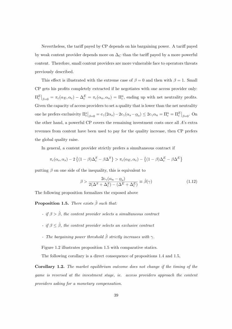
Nevertheless, the tariff payed by CP depends on his bargaining power. A tariff payed
by weak content provider depends more on ∆C than the tariff payed by a more powerful
content. Therefore, small content providers are more vulnerable face to operators threats
previously described.
This effect is illustrated with the extreme case of β = 0 and then with β = 1. Small
CP gets his profits completely extracted if he negotiates with one access provider only:
ΠEc
∣∣β=0
= πc(αE , αe) − ∆Ec = πc(αn, αn) = Πn
c , ending up with net neutrality profits.
Given the capacity of access providers to set a quality that is lower than the net neutrality
one he prefers exclusivity Πsc
∣∣β=0
= cγ(2αs)−2cγ(αs−αs) ≤ 2cγαn = Πnc = ΠE
c
∣∣β=0
. On
the other hand, a powerful CP covers the remaining investment costs once all A’s extra
revenues from content have been used to pay for the quality increase, then CP prefers
the global quality raise.
In general, a content provider strictly prefers a simultaneous contract if
πc(αs, αs) − 2(1 − β)∆S
c − β∆S> πc(αE , αe) −
(1 − β)∆E
c − β∆E
putting β on one side of the inequality, this is equivalent to
β >2cγ(αn − αs)
2(∆S + ∆Sc ) − (∆E + ∆E
c )≡ β(γ) (1.12)
The following proposition formalizes the exposed above
Proposition 1.5. There exists β such that:
- if β > β, the content provider selects a simultaneous contract
- if β ≤ β, the content provider selects an exclusive contract
- The bargaining power threshold β strictly increases with γ.
Figure 1.2 illustrates proposition 1.5 with comparative statics.
The following corollary is a direct consequence of propositions 1.4 and 1.5,
Corollary 1.2. The market equilibrium outcome does not change if the timing of the
game is reversed at the investment stage, ie. access providers approach the content
providers asking for a monetary compensation.
39
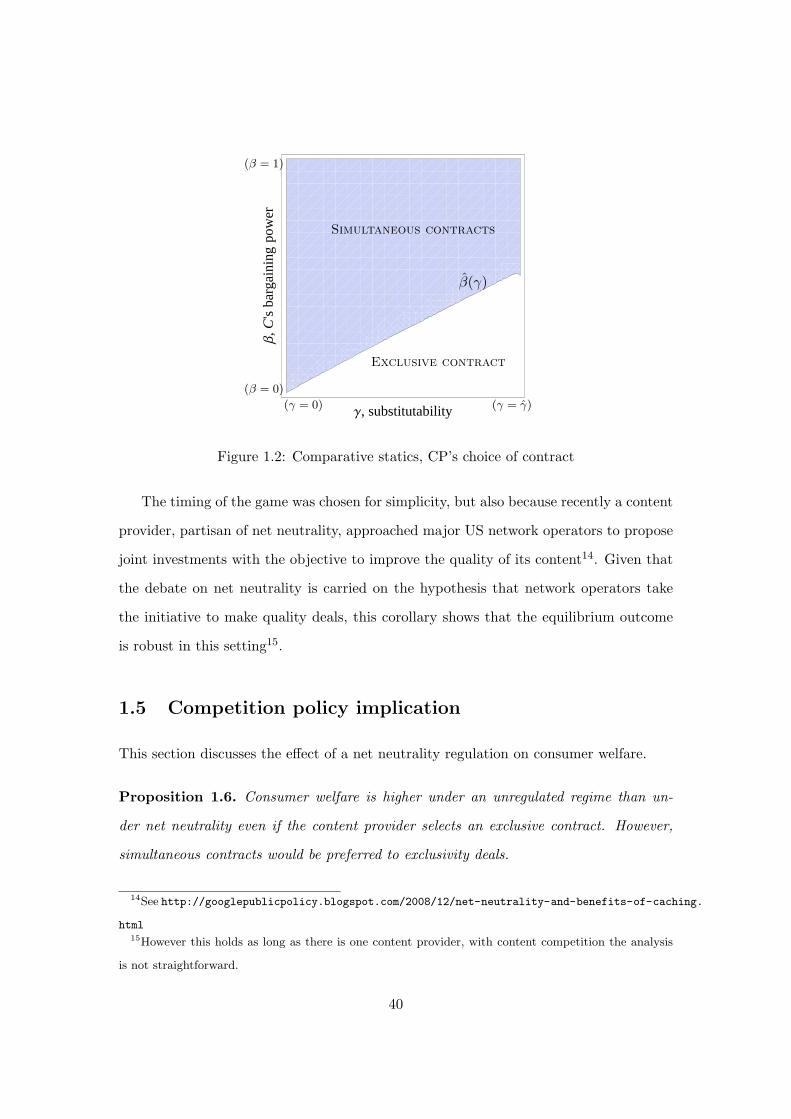
Γ, substitutability
Β,C
'sba
rgai
ning
pow
er
Exclusive contract
Simultaneous contracts
β(γ)
(γ = 0) (γ = γ)
(β = 0)
(β = 1)
Figure 1.2: Comparative statics, CP’s choice of contract
The timing of the game was chosen for simplicity, but also because recently a content
provider, partisan of net neutrality, approached major US network operators to propose
joint investments with the objective to improve the quality of its content14. Given that
the debate on net neutrality is carried on the hypothesis that network operators take
the initiative to make quality deals, this corollary shows that the equilibrium outcome
is robust in this setting15.
1.5 Competition policy implication
This section discusses the effect of a net neutrality regulation on consumer welfare.
Proposition 1.6. Consumer welfare is higher under an unregulated regime than un-
der net neutrality even if the content provider selects an exclusive contract. However,
simultaneous contracts would be preferred to exclusivity deals.
14See http://googlepublicpolicy.blogspot.com/2008/12/net-neutrality-and-benefits-of-caching.
html15However this holds as long as there is one content provider, with content competition the analysis
is not straightforward.
40
Consumer welfare is calculated as the net consumer surplus. Supposing that both
access providers set they same quality αi = αj = α, consumer surplus can be rewritten
as CS(α) = 2(α − p)q − (1 + γ)q2, where p = 1−γ2−γα is the access price at stage 2
and q = 1(1+γ)(2−γ)α is the content consumption levels at price p. Observe that with
simultaneous contracts the higher investment on quality positively impacts consumer
welfare twofold: consumption of content increases and the surplus associated with the
increased consumption of content increases as well. It is straightforward to verify that
consumers benefit from the higher quality under the non regulated regime CS(αs) >
CS(αn).
With exclusive contracts consumer welfare is still higher than with no agreements
under net neutrality. Even though the quality set by the excluded provider is lower than
the net neutrality one, the quality set by the exclusive provider compensates this loss
and demands adjust accordingly. This is a direct consequence of lemma 1.1. Given that
average quality with exclusive contracts is higher than the quality with net neutrality
total content consumption is higher with exclusive contracts than under net neutrality.
Net neutrality advocates have considered at least three versions of a net neutrality
regulation. The first one, referred as absolute non-discrimination demands that Inter-
net access providers and network operators respect the end-to-end principle, where no
network management is permitted (except for dealing with viruses and similar malicious
content), and hence no quality agreements between providers is allowed. The second
one, referred as limited discrimination without quality of service tiering is a version of
net neutrality where operators are allowed to set quality of service for different contents
but no fees are charged to content providers. These two regulatory frameworks corre-
spond to the net neutrality regime in the model and hence correspond to a lower quality
outcome, reducing consumer welfare.
The third version called limited discrimination and tiering allows agreements be-
tween content and access providers for better quality levels restricting exclusive deals
between them. This flexible regulatory framework is closest to the model except that
41

the exclusivity ban aims to avoid foreclosure issues in the content provider market. In
doing so, an Internet access provider would be compelled to open the quality service
to all content providers. An analogous regulation for the model presented in this pa-
per could be referred as content neutrality, but a regulator could not demand multiple
investments for the content provider. Nevertheless, our framework suggest a natural
policy recommendation.
The results of the model imply that competition authorities should be concerned
with small content providers. The exclusive quality deals are a consequence of the
bargaining power disadvantage they face. If access providers were constrained to setting
at least a net neutrality quality level for all content without further degrading it, content
providers would not contemplate exclusive deals and a global quality enhancement would
be agreed. It suffices to inspect condition (1.12) to remark that if the outside option
for the access providers was restricted to the net neutrality level αs ≥ αn then for all
β > 0, the content provider would enter into simultaneous agreements. If one agrees
that the quality of today’s Internet is the one made with independent investment, then
regulation could take it to be the minimal net neutrality quality benchmark and allow
only improvements.
Actually, the European Commission has recently incorporated this principle. In
November 2009 it amended its Directive on universal service and users’ rights relating
to electronic communication networks and services in order to include the article 22(3)
which stipulates that16:
In order to prevent the degradation of service and the hindering or slowing
down of traffic over networks, Member States shall ensure that national regu-
latory authorities are able to set minimum quality of service requirements on
an undertaking or undertakings providing public communications networks.
The debate on the implementation of such requirements is now expected to take place.
16See http://eur-lex.europa.eu/JOHtml.do?uri=OJ:L:2009:337:SOM:EN:HTML
42
1.6 Extensions
The section extends the basic model to consider alternative access market structure, and
the commitment assumption for the content provider.
1.6.1 Content provider with no commitment
A rather strong hypothesis in the exclusive bargaining framework is that the content
provider can commit to one access provider when offering exclusive deals. This meant
that if negotiation fails between CP , ISPi then access providers invested by their own
means, leading to net neutrality quality levels. Here, this hypothesis is relaxed allowing
the content provider to turn to the other access provider if negotiation has failed with
the first one. However it is still supposed that once negotiation has failed between an
access provider and the content provider, they cannot enter into renegotiation if the
other pair has not achieve an agreement either.
Suppose that CP chooses to deal with ISPi first. Supposing that ISPi refuses or that
they do not reach an agreement, CP turns to ISPj . If no agreement is reached between
them, then access providers set qualities equal to (αn, αn) and we are in the exclusive
dealing problem with commitment. The pair CP , ISPj sets the quality equal to αE
and the excluded provider ISPi sets a quality αe. Providers at this stage have profits
as in (1.11). This profits become then the outside option for the bargaining pair CP ,
ISPi. The bargaining pair set a contract that solves
maxαi,Ti
π(αi, αj) + Ti − Πe1−β πc(αi, αj) − Ti − ΠEc
β
with αj the quality set by ISPj that maximizes its profits maxαjπ(αj , αi). As the
resulting equilibrium qualities do not depend on the outside option, they qualities are
the same as in the other cases (αi = αE , αj = αe), and the monetary transfer is
Ti = (1 − β)πc(αE , αe) −
(πc(αE , αe) − TE
)− β π(αE , αe) − π(αe, αE)
Final profits for the content provider are
ΠE′
c = πc(αE , αe) − TE + βTE + π(αE , αe) − π(αe, αE)
43
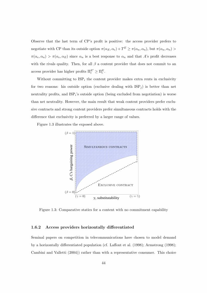
Observe that the last term of CP’s profit is positive: the access provider prefers to
negotiate with CP than its outside option π(αE , αe) +TE ≥ π(αn, αn), but π(αn, αn) >
π(αe, αn) > π(αe, αE) since αn is a best response to αn and that A’s profit decreases
with the rivals quality. Then, for all β a content provider that does not commit to an
access provider has higher profits ΠE′
c ≥ ΠEc .
Without committing to ISPi the content provider makes extra rents in exclusivity
for two reasons: his outside option (exclusive dealing with ISPj) is better than net
neutrality profits, and ISPi’s outside option (being excluded from negotiation) is worse
than net neutrality. However, the main result that weak content providers prefer exclu-
sive contracts and strong content providers prefer simultaneous contracts holds with the
difference that exclusivity is preferred by a larger range of values.
Figure 1.3 illustrates the exposed above.
Γ, substitutability
Β,C
'sba
rgai
ning
pow
er
Exclusive contract
Simultaneous contracts
(γ = 0) (γ = γ)
(β = 0)
(β = 1)
Figure 1.3: Comparative statics for a content with no commitment capability
1.6.2 Access providers horizontally differentiated
Seminal papers on competition in telecommunications have chosen to model demand
by a horizontally differentiated population (cf. Laffont et al. (1998); Armstrong (1998);
Cambini and Valletti (2004)) rather than with a representative consumer. This choice
44

of modeling is intuitively justified as a consumer has one telephone subscription only.
But the Hotelling model presents some limitations on respect to the elasticity of the
demand, for this reason the paper was presented using a linear elastic demand. However
the results are robust with un underlying Hotelling model.
In order to gain some elasticity assume now that consumers, who are uniformly
distributed on the [0, 1] segment, have a variable increasing and concave surplus of v(αi)
with αi the quality set by ISPi. The net utility of consumer located at x and choosing
ISPi is v + v(αi) − 12γ |x − xi| − pi, with v is the fixed utility of having access to the
Internet, which it is supposed to be sufficiently hight that it keeps the market covered.
The parameter γ ≥ 0 is again the competition intensity between access providers. Then
the indifferent consumer is located at
x =1
2+ γ v(αi) − pi − v(αj) + pj
Market shares for operators are q1 = x and q2 = 1 − x.
The cost structure for the access provider is as in the main model. The content
provider has increasing concave advertising revenues r(α) per consumer which reflect
the variable content consumption with quality variations.
Content and access provider’s profits from content are
πi = qipi − I(αi), πc = r(αi)qi + r(αj)qj .
Access competition For either regime, as long as the quality difference offered by
the access providers is not very big |v(αi) − v(αj)| ≤ 32γ access providers set prices at
equilibrium and have corresponding market shares equal to
p∗i = p(αi, αj) =1
2γ+v(αi) − v(αj)
3, q∗i = q(αi, αj) =
1
2+ γ
v(αi) − v(αj)
3
Remark that for independent access providers γ = 0 access providers have equal market
shares q∗i = 12 , otherwise if αi > αj then q∗i >
12 and qj <
12 . It is easier for access
providers to steal consumers as they become more substitutable.
45

Characterizing quality levels Given the convexity of the investment I and the
concavity of v and r, the equilibrium qualities for each scenario can be characterized by
the following equations
I ′(αn) =v′(αn)
3
I ′(αs) =v′(αs)
3+r′(αs)
2
I ′(αs) = 2q(αs, αs)v′(αs)
3
I ′(αE) = 2q(αE , αe)
(v′(αs)
3+r′(αs)
2
)
+ γv′(αE)
3(r(αE) − r(αe))
I ′(αe) = 2q(αe, αE)v′(αe)
3
Proposition 1.7. If competition between access providers is not too intense (γ not too
big) there exist a unique equilibrium in qualities with αe ≤ αs ≤ αn < αs ≤ αE.
The proof is straightforward as I ′ is increasing and v′ and r′ decreasing. In all,
similar results regarding the equilibrium outcome are obtained with this model.
1.7 Discussion
This paper has presented a model that studies the relations between Internet access
providers relations with a possibly powerful Internet content provider. Two regulatory
regimes where considered. A regulated one, called net neutrality where providers could
not cooperate in quality enhancement agreements. And a second one, where the content
provider could bargain with both access and obtain simultaneous quality contracts, or
with only one of them entering into quality exclusive deals.
Some of the important insights of the model reveal that small content providers face
a rather weak position when dealing with both operators simultaneously. This is given
by the capacity operators have to degrade content’s quality if no agreement is reached.
On the other hand, a very powerful content can extract access providers’ surplus leading
them to a prisoners dilemma situation where investing in quality leads them to profit
losses compared to the net neutrality regime.
46

It has been showed that an unregulated regime leads to global higher quality in-
creasing consumers welfare. Competition authorities should consequently take measures
to protect small content, but to let established popular content increase their quality
through vertical agreements.
The paper has focused on a powerful content provider because the Internet content
and services market is somehow concentrated and none of the preceding studies have
considered it. The author is aware that the problem of entry barriers of new content has
not been treated and it will be done in the near future.
1.8 Appendix: Proofs of Propositions
Proof of proposition 1.1. It is to verify that αn = 2aγ decreases with γ given that aγ
decreases with γ:
daγdγ
= −2 (4 − 2γ(1 + γ)) + γ3(3 + 2γ)
(2 − γ)3(1 + γ)2(2 + γ)2< 0
for γ ∈ [0, 1]. In general, it can be showed using the implicit function theorem for a
general convex cost function that the symmetric equilibrium decreases with competition.
The system (1.2) admits another solution where one access provider invests more
than the other:
α∗i = aγ + 2bγ −
√
aγ2 − 4bγ2, α∗
j = aγ + 2bγ +√
aγ2 − 4bγ2
this solution exists only for aγ ≥ 2bγ . This is an equilibrium as long as second order
condition holds for both operators, that is for aγ <√
5bγ . The two conditions set the
competition parameter 0.53 < γ < 0.56.
Proof of proposition 1.2. The other asymmetric equilibria profile is
α∗i = aγ + 2bγ −
√
aγ2 − 4bγ2 + 2cγ , α∗
j = aγ + 2bγ +√
aγ2 − 4bγ2 + 2cγ
with the restriction ofaγ
2+2cγ
5 < bγ2 <
aγ2+2cγ
4 , that corresponds to 0.77 < γ < 0.79.
47
Existence of equilibrium. It remains only to verify that the joint surplus is positive
and that the bargaining solution actually exists. But this follows straightforward, the
maximization program defined in (1.3) for αi = αs assures that at least ∆C + ∆A = 0,
then as αs 6= αs, the joint surplus is then positive at it is a maximizer.
Proof of proposition 1.3. It only rests to characterize the segment where access providers
share the market. The cornered market equilibrium corresponds to a situation where
the equations (1.8) and (1.9) hold with the excluded provider indifferent between leaving
the market, i.e. with Rαi (αE) = 0. This is for
αe = aγe+ bγe
, αE =(aγe
+ bγe)2
2bγe
that corresponds to γe that solves 8bγ2cγ = (aγ
2 − bγ2)(aγ
2 − 5bγ2). This last equation
sets the threshold to γe ≈ 0.319. Using simple numerical methods we can calculate the
maximal difference in qualities: αE(γe) − αe(γe) ≈ 1.618
Existence. The verification of the existence of the bargaining Nash equilibrium is
straightforward. Note that if the bargaining pair sets αi = αn the excluded access
provider would then set αj = αn, so the gain in revenues are at least zero, then ∆E +
∆Ec ≥ 0.
Proof of corollary 1.1. I show that the mean quality with simultaneous contracts is
higher than the mean quality with exclusive deals. Suppose the contrary, that αs <
αE+αe
2 . Then, given the convexity of I ′(α) = α2
2 and that I ′(0) = 0 we have that
I ′(αs) ≤ 0 +2αs
αE + αeI ′(αE + αe
2
)
≤ 2αsαE + αe
(I ′(αE)
2+I ′(αe)
2
)
Then using equations (1.6), (1.8) and (1.9)
aγαs + cγ = I ′(αs) ≤2αs
αE + αe
(I ′(αE) + I ′(αe)
2
)
=2αs
αE + αe
(aγ(αE + αe) + cγ
2
)
which implies that αE < αE + αe ≤ αs and this is not possible given that αE > αs.
In the same, when competition is not too intense and the market is not foreclosed
for the excluded access provider the average quality with exclusive deals is higher than
48

with net neutrality. Remember that for γ = 0: αe = αn < αs = αE , so αn <αE+αe
2 , and
as γ > 0, the quality lost with αe is somehow recovered with αE . It is enough to check if
the inequality holds for γ, the competition level where the excluded access provider sets
its quality at lowest before leaving the market. At this point we have that αe = aγ + bγ
and αE =(aγ+bγ)2
2bγ, but then the condition αn = 2aγ <
(aγ+bγ)(aγ+3bγ)4bγ
= αE+αe
2 holds if
0 < (aγ − 3bγ)(aγ − bγ) which is verified given that aγ ≈ 0.44 > 0.27 ≈ 3bγ .
Proof of proposition 1.4. Suppose first that the rival ISPj refuses CP’s proposal, then if
ISPi accepts the negotiation call of CP he would have exclusive contract profits ΠEA. If it
refuses to enter into negotiation its profits correspond to those in a net neutral regime.
Given that net neutrality profits correspond to the outside option of access provider
ISPi, by construction the following inequality follows
ΠE = π(αE , αe) + TE ≥ π(αn, αn) = Πn
Suppose now that the rival ISPj is willing to negotiate with CP as well. Having a
simultaneous contract with CP is a best option for ISPi than being excluded.
Πs = π(αs, αs) + TS ≥ π(αs, αs) ≥ π(αe, αE) = Πe
The first inequality holds given that by definition a successful negotiation brings profits
higher than the outside option. The second one is verified in two steps: first π(αs, αs) ≥
π(αe, αs) given that αs is a best response to αs, and second π(αe, αs) ≥ π(αe, αE)
because αs ≤ αE and the profits of ISPi decrease with the rivals quality.
Finally, suppose that the content provider is very powerful with β close to 1. First
observe that with a reasoning analog to the preceding one π(αn, αn) ≥ π(αs, αn) >
π(αs, αs). Then observe that a powerful content provider pays only TS∣∣β=1
= −∆S ,
hence access providers have higher profits with net neutrality than with the simultaneous
contracts
Πn = π(αn, αn) > π(αs, αs) = π(αs, αs) − ∆S = Πs
Proof of lemma 1.1. The proof starts with a result that will be of use:
49

Intermediary result It will be of use to first show that αE − αs < αn − αe, i.e. that
the threat point quality decreases faster than what the exclusive quality increases. This
is a general demonstration given the convexity of I ′(α).
First remark that given that αe < αn < αE we can write αn = (1− t)αe+ tαE where
t = αn−αe
αE−αe. Then using first-order conditions (1.2), (1.8) ,(1.9) and the convexity of I ′
we have that
aγαn = I ′(αn) ≤ (1−t)I ′(αe)+tI ′(αE) = aγ((1−t)αe+tαE)−bγ(αE−αe)+t(cγ+2bγ(αE−αe))
which implies that
αe +bγ(αE − αe)
cγ + 2bγ(αE − αe)(αE − αe) < αn
With the same reasoning taking αe < αs < αE the following inequality holds
αe +cγ + bγ(αE − αe)
cγ + 2bγ(αE − αe)(αE − αe) < αs
Finally adding this two inequalities we have that αE + αe < αs + αn.
Proof of (i) With the intermediate result it is straightforward to show that the surplus
made by CP is greater with simultaneous contracts.
∆sc = cγ(αs − αs) ≥ cγ(αs − αn) > cγ(αE + αe − 2αn) = ∆E
c
with equality at ∆Sc
∣∣γ=0
= αs−αn
2 = ∆Ec
∣∣γ=0
.
Proof of (ii) Writing dγ = γ2
(1−γ2)(4−γ2)2, profits from content can be rewritten as
π(αi, αj) =aγ + bγ
2α2i − bγαiαj + dγα
2j −
α3i
6
First, notice that
∆S∣∣γ=0
=
(α2s
4− α3
s
6
)
−(α2n
4− α3
n
6
)
= ∆E∣∣γ=0
50

I can conveniently use the fact that I(α) = α3
6 = α2 I
′(α)17 and using first order
conditions (1.2), (1.6), (1.8) and (1.9) profits can be rewritten and
∆E =aγ + bγ
6(α2
E − α2n) −
2bγ3
(αEαe − α2n) −
cγ3αE − dγ(α
2n − α2
e)
∆S =aγ + bγ
6(α2
s − α2s) −
2bγ3αs(αs − αs) −
cγ3αs
Comparing this two expressions is straightforward.
Proof of proposition 1.6. I show that consumer surplus without regulation but with ex-
clusive contracts is higher than consumer surplus with no investments, but smaller than
with simultaneous quality enhance contracts:
CS(αn, αn) < CS(αE , αe) < CS(αs, αs)
Recall that consumer surplus is
CS = u(q1, q2) − p1q1 − p2q2
using equilibrium prices given by (1.1), we can simplify the above expression to
CS =1
(2 − γ)2(1 + γ)
(4 − 3γ2
2(2 + γ)2(1 − γ)(αi − αj)
2 + αiαj
)
It is then sufficient to show that:
α2n ≤ 4 − 3γ2
2(2 + γ)2(1 − γ)(αE − αe)
2 + αEαe ≤ α2s.
By corollary 4, αn <αE+αe
2 , which implies that
α2n <
(αE + αe)2
4=
1
4(αE − αe)
2 + αEαe <4 − 3γ2
2(2 + γ)2(1 − γ)(αE − αe)
2 + αEαe
given that 4−3γ2
2(2+γ)2(1−γ)≥ 1
2 for all γ ∈ [0, 1]. Then the left side of the inequality holds.
For the right side, first observe that for γ = 0 the inequality holds: 12(αs − αn)
2 +
αsαn < α2s. Then observe that for 0 < γ < γe, using Corollary 1.1
α2s > (αE + αe − αn)
2 >4 − 3γ2
2(2 + γ)2(1 − γ)(αE − αe)
2 + αEαe
17but with general convex costs the same results hold
51

given that 4−3γ2
2(2+γ)2(1−γ)< 2
3 for γ < γe.
52

Bibliography
Allain, M. L., and Chambolle, C. (2007). Anti-competitive effects of resale-bellow-cost
laws. Cahier de Recherche de l’Ecole Polytechnique no. 2009-09. Available at http:
//ideas.repec.org/p/hal/wpaper/hal-00367492_v1.html.
Armstrong, M. (1998). Network Interconnection in Telecommunications. The Economic
Journal, 108(448), pp. 545-564.
Binmore, K., Rubinstein, A., and Wolinsky, A. (1986). The Nash Bargaining Solution
in Economic Modelling. The RAND Journal of Economics, 17(2), pp. 176-188.
Cambini, C., and Valletti, T. M. (2004). Access charges and quality choice in competing
networks. Information Economics and Policy, 16(3), pp. 391-409.
Cheng, H. K., Bandyopadhyay, S., and Guo, H. (2011). The Debate on Net Neutrality:
A Policy Perspective. Forthcoming in Information Systems Research, 22(1). Available
at http://ssrn.com/abstract=959944.
Choi, J. P., and Kim, B. C. (2010). Net Neutrality and Investment Incentives. The
RAND Journal of Economics, 41(3), pp 472-597.
Cremer, J., and Riordan, M. H. (1987). On governing multilateral transactions with
bilateral contracts. The RAND Journal of Economics, 18(3), pp. 436-451.
Economides, N., and Tag, J. (2007). Net neutrality on the Internet: A two-sided market
analysis. NET Institute Working Paper No 07-45. Available at http://ssrn.com/
abstract=101912.
53

Faulhaber, G. R., and Hogendorn, C. (2000). The market structure of broadband
telecommunications. The Journal of Industrial Economics, 48(3), pp. 305-329.
Fijnvandraat, M., and Bouwuman, H. (2006). Flexibility and broadband evolution.
Telecommunications Policy, 30, pp. 424-444.
Hermalin, B. E., and Katz, M. L. (2007). The economics of product-line restrictions with
applications to the network neutrality debate. Information Economics and Policy,
19(2), pp. 215-248.
Horn, H., and Wolinsky, A. (1988). Bilateral monopolies and incentives for merger. The
RAND Journal of Economics, 19(3), pp. 409-419.
Kocsis, V., and de Bijl, P. (2007). Network neutrality and the nature of competition
between operators. International Economics and Economic Policy, 4(2), pp. 159-184.
Laffont, J. J., Rey, P., and Tirole, J. (1998). Network competition: I. overview and
nondiscriminatory pricing. The RAND Journal of Economics, 29(1), pp. 1-37.
McAfee, P., and Schwartz, M. (1994). Opportunism in Multilateral Vertical Contract-
ing: Nondiscrimination, Exclusivity, and Uniformity. The American Economic Review,
84(1), pp. 210-230.
Milliou, C., and Petrakis, E. (2007). Upstream horizontal mergers, vertical contracts.
International Journal of Industrial Organization, 25(5), pp. 963-987.
O’Brien, D. P., and Shaffer, G. (1992). Vertical control with bilateral contracts. The
RAND Journal of Economics, 23(3), pp. 299-308.
54
Chapter 2
Investment with commitment
contracts: the role of uncertainty
2.1 Introduction
Infrastructure industries have experienced an essential change in regulation. More than
thirty years ago, firms in these industries were considered natural monopolies and were
therefore protected from entry but subject to rate of return regulation. Nowadays compe-
tition is actively promoted in many countries and infrastructure-based firms face several
forms of incentive regulation.
The passage from a natural monopoly to market competition was made by man-
dating access to the incumbent firm’s infrastructure. This infrastructure was in most
countries a heritage of the formerly State-owned monopoly. Technological progress and
the increasing utilization of network will require the upgrade and eventually the ren-
ovation of this inherited infrastructure. In telecommunications, the roll-out of Next
Generation Access networks (“NGA networks”) based on fibre optic cable is aspired to
replace cooper-based broadband services.
Anticipating the replication of a monopoly infrastructure, regulatory authorities will
likely apply ex ante regulation for whoever builds a network. For instance, the Eu-
55

ropean Commissions guidelines draft for regulation of next generation access networks
encompass mandated access for operators that roll out fibre optic networks.1
Fostering retail market competition without hindering investment can be a challeng-
ing objective. The economics literature on R&D rivalry and adoption of new technology
has pointed out that if a firm suffers a profit reduction when its rival innovates then
a firm has incentives to be the first one to adopt the new technology and win the in-
vestment race. However when imitation is possible and the profit reduction effect is not
significant, there is a second-mover advantage as firms wait for others to incur R&D
fixed costs and then imitate; as a consequence investment is delayed, see Katz and
Shapiro (1987).2 Mandating access to firms in network industries that drastically re-
duces investment profits can induce the same late adoption effect. In particular, when
industries are characterized by the irreversibility of much of the infrastructure cost and
by risk due to uncertainty on future profits, firms are not willing to invest if access policy
asymmetrically allocates the risk to the firm that invests first.
The industrial organization literature on the impact of access regulation on broad-
band investment takes three approaches.3 Fist, a body of literature focuses on asymmet-
ric frameworks where an entrant who enjoys regulated access to the incumbent’s network
invest and builds its own network (see Bourreau and Dogan (2005); Cave (2006); Schutz
and Tregouet (2008), etc.). A second body of literature studies the incentives of an in-
cumbent to upgrade its network when subject to mandated access (see Kotakorpi (2006);
Camacho and Menezes (2009); Nitsche and Wiethaus (2010)) The third body of litera-
1See the European Commission draft recommendation on regulated access to Next Generation
Access Networks available at: http://ec.europa.eu/information_society/policy/ecomm/library/
public_consult/nga and http://ec.europa.eu/information_society/policy/ecomm/library/
public_consult/nga_2.2This is the case if most of the investment has to be done only once and not continuously. When
innovation is sequential and consecutive it has been recently demonstrated that imitation has a positive
effect on innovative outcomes, see Bessen and Maskin (2009). One can agree that the roll-out of NGA
networks corresponds mainly to a fixed investment.3See Cambini and Jiang (2009) for a literature review on broadband investment and regulation.
56

ture, which is the closest to our purpose, focuses on a more symmetric situation where
both the former incumbent and entrant must build the network from “scratch”. In this
literature, inspired from the patent race work, the incumbent role is endogenous to the
model (see Vareda and Hoernig (2009); Hori and Mizuno (2006, 2009); Gans (2001)).
The object of study is then to determine if investment is timely when firms know that
access to their network will be mandated. In general, it finds that with high access
charges first investment is made earlier than with low access charges. The regulatory
authority must then compromise static efficiency in order to induce early investment.
This paper studies the private incentives to invest on a new network when it cannot
be financed by direct subsidies and revenues from the market are the only source of
funding. Concisely, it finds that for adverse market configurations, more sophisticated
access contracts including commitment clauses between firms can be more efficient than
simple linear wholesale access tariffs.
Section 2.2 describes the model of two ex ante symmetric firms that must make
an irreversible investment decision while facing future uncertain profits together with
possible access obligations. Section 2.3 builds the benchmark of perfect information on
future profits to illustrate the effect of the access charge level on the equilibrium out-
come. As highlighted by the literature, for example by Bourreau and Dogan (2005), low
access charges induce service-based competition, whereas high access charges encourage
facilities-based competition as long as profits are high enough to cover fixed costs for
both firms.
Section 2.4 introduces uncertainty on future market profitability. With unknown
future profits, firms delay investment when they know rivals are willing to invest. In
effect, mandated access policies, as Guthrie (2006) points out, gives “investment flexi-
bility” to firms: they invest in realized good states and seek access in bad states. Given
that industry profits are revealed only when one of the firms has invested, it is prof-
itable to delay investment waiting for the other firm to incur the sunk cost. As a result,
uncertain profits combined with mandated access policies do not induce simultaneous
57

“timely” investment.
If the roll-out of NGA is desired, the wholesale price must be sufficiently high to
encourage one of the firms to invest first.
Section 2.5 characterizes the market configuration induced by a linear wholesale price
set by the regulator prior to investment decisions. Again, with a low access charge the
firm that has delayed investment will seek access instead of building its own network in
good and bad states. Whereas with a higher access charge, the firm that has delayed the
deployment of the network will continue to seek access if the industry is revealed not very
profitable, but it will bypass the firm that has invested first in good states by rolling out
its network. This opportunistic behaviour reduces the expected wholesale profit for the
firm that has invested first. Given anticipated rent losses in good states, a firm will roll
out the network only if it is further compensated for bearing all the risk. Considering
this, the literature and authorities have introduced the notion of “risk premium” access
charges: a wholesale mark-up aimed at compensating the investing firm, see Pindyck
(2007).
However, when the sunk cost is rather high and industry profits are expected to be
low, a firm anticipating the wholesale rent reduction in good states will no longer be
willing to invest even if monopoly rents are allowed in bad states. Then, only a firm in
monopoly would incur the sunk cost.
Long-term contracts or contracts with commitment clauses have been used in other
industries for a better risk management. For example, long-term contracts in electric-
ity generation markets are used to encourage entry by creating reliance on long-term
relationships c.f. Onofri (2003). They have also been used in the telecommunications
industry for quite a while. They are usually agreements to best cope with heavy invest-
ment like transoceanic fiber optic deployments, they are known as Indefeasible rights
of use (IRU) aggrements. This idea is then applied to NGA investment. If the rival
firm contractually commits to seeking access in either state, then the firm that would
had otherwise not invested secures wholesale profits that cover the sunk cost, solving
58

the hold-up problem. Similarly, an access contract with commitment clauses allows a
reduction of the risk premium wholesale price. The network-providing firm renounces to
higher wholesale revenues in bad states by assuring wholesale revenues in good states.
The network-seeking firm gives up facilities-based rents in good states for a lower access
charge in bad ones. The paper shows that ex ante commitment clauses between firms
can be beneficial even if firms privately agree on the wholesale price access level.
2.2 The model
Consider two risk-neutral identical firms that plan to enter into an infrastructure-based
industry. The firms need a network facility to be able to compete in the retail market.
A firm builds its facility at a fixed sunk cost I > 0, investment costs on infrastructure
are considered irreversible. However, it is not necessary that both firms deploy a network
in order to compete in the retail market. The firm without a network may use its rival’s
network to provide the service in exchange of a usage-based access charge w ≥ c, where
c ≥ 0 is the infrastructure usage costs. For simplicity, other retail costs are normalized
to zero.
Industry profit flows are uncertain for both firms as well as for the regulator until
investment is made. This could be, for example, due to uncertainty on future demand
or due to common exogenous industry shocks. This simple model supposes that the
variation of profit flows is reduced to two possible states of the world: a good or optimal
state, represented by the parameter θH , which occurs with probability µ ∈ [0, 1]; and
a bad or adverse state, represented by the parameter θL such that 0 < θL < θH ≤ 2.4
The state of the world is revealed only when at least one of the firms has rolled out
the infrastructure. If none of the firms invests, the service is not provided and profits
from the service provision remain of course uncertain. The model assumes that the
opportunity cost of providing the service is normalized to zero.
4We suppose that θH ≤ 2 in order to have welfare decrease with the access charge. See section 2.3.1
for details.
59

Throughout the paper, firms compete in the retail market by setting downstream
capacities, i.e. with Cournot competition. The model uses a simple linear inverse demand
function p = 1 −Q, with Q = q1 + q2 the total downstream capacity.5
If only one firm has rolled out the infrastructure profits are asymmetric. The profit
for the firm that has invested, who will be called from now on the network provider, is
ΠP = θ q1(p− c) + q2(w − c) − I
with q1 its downstream capacity, and q2 its rival’s capacity. The profit for the other firm,
called the network seeker, is then
ΠS = θ q2(p− w)
For both firms the exogenous industry shock θ = θH , θL is set according to nature.6
If both firms build their facilities, profits are symmetric and equal to
ΠC = θ qi(p− c) − I
Firms need two periods to build a network from scratch. The first period is used
to undertake the necessary civil engineering work and the second to lay out cables and
other necessary equipment. If one firm has a built civil infrastructure, as regulation
contemplates, must give access to ducts and conduits for other firms to lay out the
optical equipment.7
The timing of the game is as follows:
0. Nature privately sets the state θH or θL
5The model can be adapted to price competition in the downstream market. Once firms set their
quantities at equilibrium, the profit flows that depend on the access charge have equivalent properties.
The Cournot competition can be interpreted as capacity on selling the final service: advertising, points
of sale, etc.6The basic structure of profits in the model is inspired from Hori and Mizuno (2006, 2009).7Supposing that firms need two periods to build a network greatly simplifies the structure and the
resolution of the game. See the appendix for a graphical representation of the game tree.
60

1. The regulator sets the mandatory access conditions.
2. Firms simultaneously decide to invest or to delay investment. If at least one firm
has invested, the state of the world is revealed.
3. If only one firm invested, the firm that delayed investment observes the announced
state of the world and chooses:
- To invest and deploy its own network or bypass the firm.
- To not dot invest and seek access to the competitor’s network.
If both firms have invested in stage 2., they continue with the roll out of the
network.
If both of them have decided to delay investment, they can decide to invest now,
but none of them would make profits in stage 4.
4. Firms compete in the retail market.
2.2.1 Retail market competition
In the last stage, firms set their downstream capacity, which determines the margins
over variable costs corresponding to the non-stochastic part of the firms profits. Cournot
equilibrium is standard.
Service-based competition (SBC) If only one firm has rolled out a network, profits
at equilibrium are
ΠP (w, θ) = θπp(w) − I (2.1)
ΠS(w, θ) = θπs(w)
Where πp(w) = (1−2c+w)2
9 + (w−c)(1−2w+c)3 , and πs(w) = (1−2w+c)2
9 are the non-stochastic
part of profits.
The market is shared by both firms as long as the access charge is not higher than
wm = 1+c2 which is the access charge that the network provider would have set to
61

maximize its profits and corner the other firm. For future reference, denote by πm =
(1−c)2
4 profit flows of the vertical integrated firm in monopoly. The profit in monopoly
is ΠM (θ) = θπm − I.
Facilities-based competition (FBC) If both firms have rolled out a network, equi-
librium margins over variable costs are symmetric and equal to πc = (1−c)2
9 , total profits
are
ΠC(θ) = θπc − I (2.2)
These profit flow functions at retail equilibrium have some natural intuitive properties.
First, profits for the network provider increase with the access charge, whereas they
decrease for the network seeker. Second, profit flows for the access provider are superior
to profit flows for the access seeker as long as the access charge is above marginal
costs. Third, access charges at marginal cost set zero wholesale margins for the network
provider and firms have the same profit flow as in facilities-based competition. Finally,
the difference in margins set by an access charge w > c between firms is represented by
the following relation:
πp(w) − πcπc − πs(w)
=5
4(2.3)
Note as well the relation between profit flows in competition and in monopoly
πm =9
4πc.
2.3 Benchmark: Perfect information
2.3.1 Welfare
Social welfare is defined by the sum of profits and consumer surplus minus costs. For a
given θ, welfare in service-based competition is
WSBC(w, θ) = CS(w) + θ (πp(w) + πs(w)) − I
where consumer surplus is CS(w) = (2−w−c)2
18 . One can readily verify that welfare
decreases with the access charge as long as θH ≤ 2.
62

With facilities-based competition welfare is
WFBC(θ) = CSc + 2θπc − 2I + φ
where CSc = 2(1−c)2
9 is the consumer surplus and φ ≥ 0 encompasses the expected
dynamic benefits of FBC that our static framework cannot explicitly describe. In effect,
FBC is expected to remove heavy regulation requirements in the industry and it is widely
accepted as a necessary condition for long-term efficiency.
Other than the dynamic efficiency gains, observe that consumers enjoy a higher
surplus with FBC than in SBC if the access charge is above network costs w > c. However
they enjoy the same surplus if the access charge equals marginal costs CSc = CS(c).
Similarly if w = c profit flows for the access provider and access seeker equal FBC profit
flows πp(c) = πs(c) = πc. Then, if investment is possible with w = c, a social planner
opts for SBC if φ < I. If the access charge is w > c, then is socially preferable to have
FBC if infrastructure costs are low and SBC otherwise.
Figure 2.1 can be understood in terms of geographical density. In urban areas de-
ployment costs are rather low compared to rural areas.
I0 FBC
WFBC > WSBC(w)
SBC
WSBC(w) > 0
no infrastructure
WSBC(w) < 0
Figure 2.1: Preferred type of competition when no subventions are allowed.
As a general rule, if the regulator promotes SBC, it will do so by setting the lowest
access charge that induces investment.
We are interested in the particular range of values where FBC competition is viable
only in a good state of the world:
ΠC(θH) ≥ 0 ≥ ΠC(θL) (2.4)
This condition bounds throughout the paper the range of investment costs of interest
I ≡ θLπc ≤ I ≤ θHπc ≡ I .
63

2.3.2 Equilibrium with perfect information
This section develops the reference point for the incomplete information game. With
perfect information both the regulator and the firms know the state of the world, ie.
future industry profits. Yet the regulator has the availability to determine the market
outcome according to the access charge he sets in the first stage of the game.
Suppose first that the state of the world is θL. If one firms has invested at stage 2,
the other firm chooses to seek access at stage 3 given that bypassing leads to negative
profits. Then, the investment game at stage 2 can be represented by the matrix:
Invest Delay investment
Invest ΠC(θL) , ΠC(θL) ΠP(w, θL) , ΠS(w, θL)
Delay investment ΠS(w, θL) , ΠP(w, θL) 0 , 0
for all access charge c ≤ w ≤ wm set by the social planner.
In a bad state of the world the only possible equilibrium is SBC as long as the firm
that invests makes no deficit ΠP (w, θL) ≥ 0. We suppose that if firms are indifferent
between investing and not investing, they invest. In this way, the regulator can induce
the roll-out of at least a network by setting w ≥ wL, where wL saturates the budget
constraint ΠP (wL, θL) = 0. This access charge can be explicitly calculated:
wL = wm − 3
√
θLπm − I
5θL
The access charge that encourages investment reduces monopoly profits for the net-
work provider as it lowers the tariff he would have set otherwise in an unregulated en-
vironment: wm the monopoly foreclosing access charge. Remark that regulated service-
based competition is viable in a bad state as long as investment is feasible for a firm in
monopoly in a bad state, that is, the radical of the above expression is real.
In a good state θH , the regulator can decide which market configuration he promotes.
Denote by w the access charge that makes a firm indifferent between bypassing and
64

seeking access (provided the other one has invested): ΠC(θH) = ΠS(w, θH). Explicitly,
w = wm − 3
√
θHπc − I
4θH(2.5)
By setting a “high” access price w ≥ w we have that ΠC(θH) ≥ ΠS(w, θH). Then
given that one firm has invested in stage 2, its rival faced to the choice of bypassing or
seeking access will bypass. In this way, FBC is the equilibrium induced by the regulator.8
Whereas with a “low” access charge c ≤ w < w, a firm seeks to have access to rival’s
network - provided that there is one - if given the option of bypassing or seeking access.
By replacing θL for θH , the matrix represented above describes the game at stage 2 in a
good state of the world. It is straightforward to verify that in a good state a firm invests
at marginal cost ΠP (c, θH) = θHπp(c)− I = θHπc− I ≥ 0. Then SBC is the equilibrium
of the game.
Bourreau and Dogan (2005) were among the first to formalize the idea that if the
regulator wishes to encourage facilities-based competition, access charges should not be
too low. The exposed above is resumed in the following lemma.
Conclusion 2.1. Suppose that firms and the regulator have knowledge of the state of
the world.
- In θL, the equilibrium is SBC if the access charge is wL.
- In θH , if the access charge equals c then the equilibrium is SBC. If on the other
hand the access charge is set to w, the equilibrium is FBC.
2.4 Uncertainty
This section describes in more detail the investment game under uncertainty and it
shows, as the previous section, how the access charge set by the regulator can create
investment incentives and, consequently, determines the market equilibrium outcome.
8Note that this outcome is obtained either by both firms investing at stage 2, or by a sequential
investment in stages 2 and 3.
65

Suppose that at stage 2 one firm invests and the other one delays investment. As
developed in the previous section, the decision of the firm that has delayed investment
in stage 3 depends on the access charge level.
If w ≥ w, the firm that has delayed investment chooses between “seeking access”
or “bypassing” while having full information of the state of the world. In a good state
it bypasses and in a bad state it seeks access. Its expected profits at stage 2 are then
µΠC(θH) + (1 − µ)ΠS(w, θL). The expected profits for the firm that invests in stage 2
are µΠC(θH) + (1 − µ)ΠS(w, θL).
If on the other hand the access charge is low c ≤ w < w, then in either state
of the world the firm that delays investment bypasses. Its expected profits are then
µΠS(w, θH) + (1− µ)ΠS(w, θL), and consequently the firm that invests at stage 2 is the
access provider for either case, expecting profits µΠP (w, θH) + (1 − µ)ΠP (w, θL).
In sum, the expected payoffs for the firms that invests first are
XI(w) =
µΠP (w, θH) + (1 − µ)ΠP (w, θL), c ≤ w < w
µΠC(θH) + (1 − µ)ΠP (w, θL), w ≤ w ≤ wm
(2.6)
and for the firm that delays investment:
XD(w) =
µΠS(w, θH) + (1 − µ)ΠS(w, θL), c ≤ w < w
µΠC(θH) + (1 − µ)ΠS(w, θL), w ≤ w ≤ wm
(2.7)
Considering this, the game in stage 2 can be rewritten in normal form
Invest Delay investment
Invest E[ΠC(θ)] , E[ΠC(θ)] XI(w) , XD(w)
Delay investment XD(w) , XI(w) 0 , 0
where E[ΠC(θ)] = µΠC(θH) + (1 − µ)ΠC(θL) is the expected gain in facilities-based
competition.
The strategic form representation of the game allows us to determine the effect of
the access terms on the equilibrium outcome of this investment game.
66

Observe first that in this simplified framework, firms face a second-mover advantage.
In other words, the best response to “Invest” is to “Delay investment”. In effect, after a
firm has rolled out its network, it is mandated to open it for firms that delay investment.
This gives, as Guthrie (2006) calls, “investment flexibility” to coming entrants. It is
profitable for firms to wait for the other firm to commit to invest and to have industry
profits revealed before deciding how to enter the market. Consequently, firms facing
uncertainty will unlikely invest simultaneously. Proposition 2.1 follows.
Proposition 2.1. E[ΠC(θ)] < XD(w) for all w ≤ wm. In other words, if facilities-based
competition is only feasible in an optimal state of the world then Invest, Invest is not
equilibrium for any access charge.
Proof. See the appendix for all proofs.
If the construction of at least one infrastructure is desired, the regulator needs to
encourage one of the firms to lead investment and obtain a Invest, Delay investment
equilibrium. Formally, in this model, the access charge that guarantees some form of
investment must set the expected profit of the investing firm higher than its delaying
option XI(w) ≥ 0.
2.5 Access charge levels and the role of commitment
This section analyses in more detail the equilibrium of the investment game. It char-
acterizes the access charges that encourage investment, and most importantly, it argues
that in some cases a commitment clause between the investing firm and its rival is the
only way to have market competition and investment.
2.5.1 Access tariffs that induce investment
As suggested in the previous section, there are two possible equilibria where the market
develops and some form of competition is preserved.
67

In the first one, with a low access charge, only one firm invests having service-based
competition in any state of the world, call it SBC-equilibrium. The access charge that
induces it must guarantee an expected non-negative profit for the network provider:
wSBC = minw ∈ [c, w) | XI(w) = E[ΠP (w, θ)] ≥ 0
Fix µ the probability of a good state, and write E[θ] = µθH + (1 − µ)θL the mean of
the stochastic part of profit. Our simple framework allows for an explicit computation
of the SBC-equilibrium tariff:
wSBC =
c, I < ISBC
wm − 3√
E[θ]πm−I5E[θ] ISBC < I ≤ ISBC
where
ISBC =4
9E[θ]πm and ISBC =
16
9
(θHE[θ]
4θH − 5E[θ]
)
πm.
The second equilibria can go either way, FBC in a realized good state and SBC in a
bad state. Write it xBC-equilibrium, the wholesale tariff that induces it is the solution
of
wxBC = minw ∈ [w, wm) | XI(w) = E[ΠP (w, θ)] − µ
(ΠP (w, θH) − ΠC(θH)
)≥ 0
Observe that wxBC must account for the wholesale profit reduction in good states. This
gives a mark-up to the wholesale price that the literature has called “risk premium”. In
other words, it is necessary to set an access charge that compensates the “leading” firm
for the opportunistic behavior of rivals. As Guthrie (2006) and Pindyck (2007) point
out, the “leading” firm bears all of the downside risk and it must be compensated.
The xBC access tariff can be explicitly calculated:
wxBC =
w, I < IxBC
wm − 3
√
15
(
πm − I−µθHπc
(1−µ)θL
)
, IxBC(µ) < I ≤ IxBC
where
IxBC =16
9
(θHE[θ]
4θH − 5(1 − µ)θL
)
πm and IxBC =1
9(4µθH + 9(1 − µ)θL)πm.
68

Naturally, access charges increase with the cost of the network. For low infrastructure
costs, they take the lowest value. In the SBC equilibrium retail profits cover fixed
costs and it is sufficient to set the wholesale tariff equal to marginal costs wSBC = c.
Whereas for the xBC equilibrium, the “risk premium” access charge exceeds marginal
costs wxBC = w > c. See Figure 2.2 for an illustration of the access charges.
Fixed cost
Access charge
c
wm
w
wSBC
wxBC
I IISBCIxBC
Figure 2.2: Access charges in function of the fixed cost. Parameters are c = 0, µ = 0.2,
θH = 2, θL = 0.5.
With low sunk costs, both firms make some profits. For higher costs the budget
condition is saturated for the firm that invests first, whereas the other firm makes some
profits. For even higher costs, it might be that investment is not feasible.
When firms do not invest The highest cost at which a firm invests in a xBC-
equilibrium is IxBC . In effect, wxBC(IxBC) = wm, in a bad state the network provider
is in monopoly. For higher investment costs I > IxBC , the expected profit for leading
firm is negative, XI < 0.
At the SBC-equilibrium, the maximal feasible network cost ISBC is defined by the
access charge threshold w. Whenever w ≥ w, we have an xBC-equilibrium and the
expected profits are negative for the firm that invests first if w < wxBC . This is illustrated
69

in Figure 2.2.
Firms invest (for all µ ∈ [0, 1]) in the interval [I, I] whenever the impact of the
stochastic part on profits is not important and the following condition does not hold:
θHθL
>πpπc
=9
4(2.8)
When this condition holds the investment upper limit is bellow I for low values of µ.
Then we have, as illustrated in Figure 2.2, that the xBC-equilibrium is not feasible in
the interval [IxBC , I] and the SBC-equilibrium is not feasible in the interval [IxBC , I].
Monopoly investment We are interested to compare the regulated access charge
scenario with the natural monopoly9 framework. This gives us a benchmark to the
upper limit infrastructure costs to which a private investment is possible without public
funding.
A natural monopoly has expected profits equal to E[ΠM ] = µ(θHπm − I) + (1 −
µ)(θLπm− I). Then, a monopoly invests if I ≤ IM = E[θ]πm. Observe that if condition
(2.8) holds, then IM < I for low values of µ.
We conclude this section with an important remark. For costs in the interval
[ISBC , IM ], the expected payoff of a firm that serves as access provider in all states
of nature is positive only for access charges exceeding the threshold w. Nevertheless,
no firm is willing to invest because it anticipates that at this access charge, the com-
petitor would bypass instead of buying access in a good state. Access contracts with
commitment clauses are, in this situation, virtuous.
2.5.2 The role of commitment
Suppose that for a given µ the market configuration is adverse (a relatively expensive
network compared to expected profits) such that no investing equilibrium is feasible but
a firm in monopoly would invest,
IM ≥ I > maxISBC , IxBC
(2.9)
9That is, a firm that has exclusive rights over the territory to serve the market.
70
Such configurations are particularly challenging. Conciliating private investment and
market competition seems incompatible. The lack of investment is closely related to the
hold-up problem for suboptimal investment. In general, it can be solved with ex ante
commitment contracts.
In particular, if firms could contract before investment decisions are made, then a
firm committing to another to buy access during good and bad states allows to extends
the range of feasible costs up to the maximal feasible private investment level IM . In
effect, consider commitment contracts of the form w,F, where w is the linear access
payed by the access seeker in any state of the world, and F is a compensation fixed
payment in case of non-fulfillment of the commitment clause.
Commitment contract when no network is deployed When the cost of invest-
ment is high and condition (2.9) holds neither firm is willing to invest in a regulated
market: Delay investment, Delay investment is the equilibrium of the game. They
both have reservation profits equal to zero.
If firms were to agree ex ante to an access charge, it must be set at a level that
both firms obtain non-negative profits. Write wic the minimal access charge that the
network provider is willing to accept E[ΠP (wic, θ)] = E[θ]πp(wic)− I = 0, and wm. The
maximal access charge that the network seeker is willing to pay is the monopolistic one
E[ΠS(wm, θ)] = E[θ]πs(wm) = 0.
We show that there exists a range of access charges, [wic, wm], for which both firms
expect positive profits. In effect,
πp(wic) − πcπc − πs(wm)
=
IE[θ] − πc
πc − 0=
I49E[θ]πm
− 1 <5
4
which holds as long as monopoly investment is feasible. Given relation (2.3) and that
πp is increasing we have that wic < wm.
The non-fulfillment fixed payment is set to avoid opportunistic behavior. For exam-
ple, for the wholesale tariff chosen, it is sufficient to set F > ΠC(θH) − ΠS(w, θH).
The level of the access charge in a contract with commitment clauses in [wic, wm] can
71

be negotiated between firms (as discussed in the next section) or it can be determined
by the regulator. To be precise, we should no longer refer to a commitment contract
but to an infrastructure monopoly franchise if the regulator sets the access charge level
and forbids the duplication of the infrastructure immediately after industry profits are
revealed. In this case, the regulated wholesale tariff can be exactly wic. In any case, the
tariff will be lower than the monopoly access charge that leads monopoly retail prices.
The proposition summarizes the discussion.
Proposition 2.2. Access contracts with commitment clauses between firms are one an-
swer to the dilemma of preserving market competition and encouraging investment in
adverse market configurations.
Fixed cost
Access charge
Extended zoneof investment
c
wm
w
wSBC
wxBC
wic
I IIMISBCIxBC
Figure 2.3: All access charges in the gray zone [wic, wm] extend the zone of possible
investment. Parameters are c = 0, µ = 0.15, θH = 2, θL = 0.5.
Commitment contracts that reduce access charges Another adverse market con-
figuration is given when, with excessively high access prices, the only possible outcome
is the xBC-equilibrium. It could be that,
IxBC ≥ I > ISBC (2.10)
High wholesale prices result in high detail prices, which significantly reduce consumer
surplus. At the expense of facilities-based competition, a commitment contract could
72

be then more efficient given that access charges can be considerably reduced. With a
lower access price, the profit for the network seeker increase in bad states. If they are
sufficiently lowered, its expected profit exceeds that in the xBC-equilibrium. For the
network provider, gains come in good states at the expense of lower upstream profits.
Actually, there is room for gain for both firms. The proposition follows.
Proposition 2.3. If the only possible investment equilibrium is xBC, and if it requires a
high wholesale price, then commitment clauses allow to lower access charges improving
static efficiency. In particular, there exists a range of wholesale prices that are incentive
compatible for both firms.
Proof. See the appendix.
Fixed cost
Access charge
Extended zoneof investment
c
wm
w
wSBC
wxBC
I IIMISBC IxBC
Figure 2.4: All access charges in the gray zone [wic, wxBC ] are lower than the access
charge wxBC , which increases static surplus. Parameters are c = 0, µ = 0.05, θH = 2,
θL = 0.5.
The trade-off between static efficiency (lower access charges) and dynamic efficiency
(investment, facilities-based competition in good states) will be analyzed in section 2.6.
The message of this section is clear: access contracts with commitment clauses can be
beneficial in adverse market configurations as they either encourage investment where
otherwise would have not been made, and they reduce wholesale price.
73
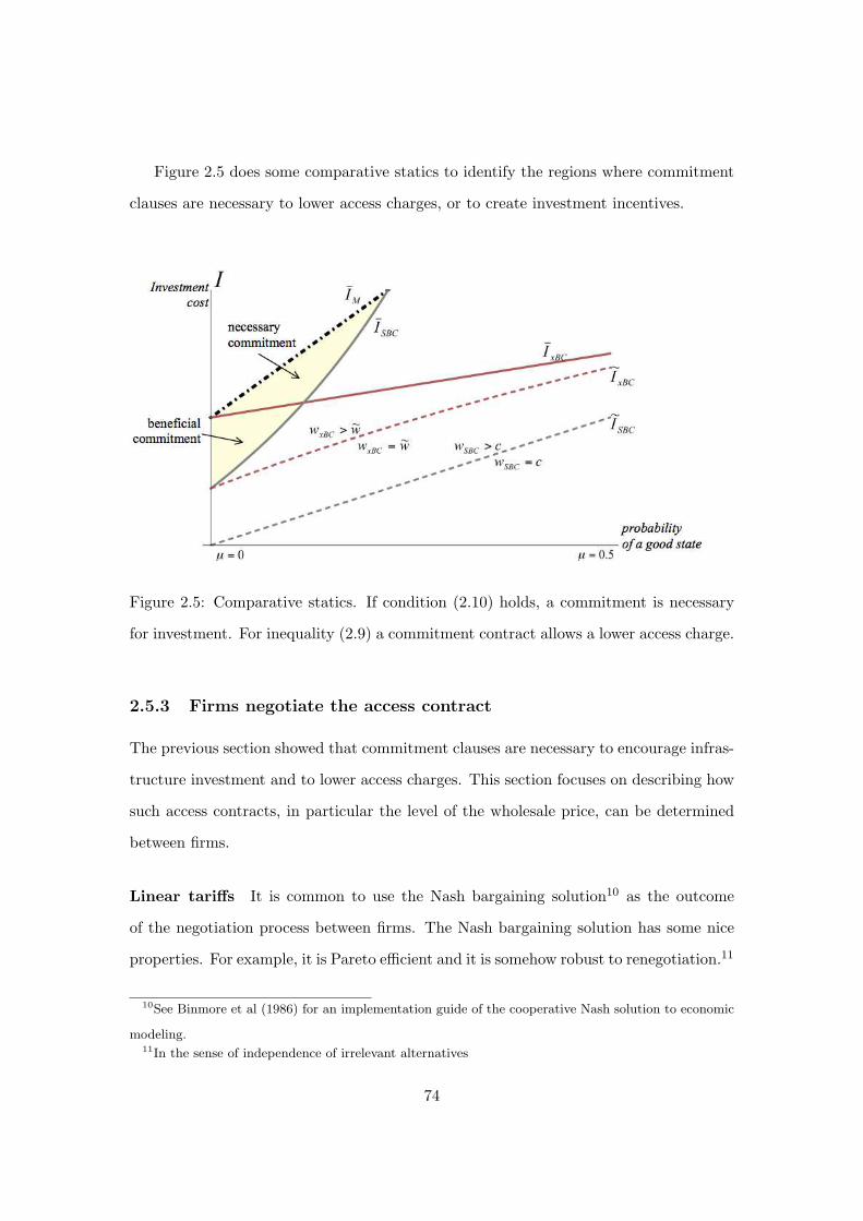
Figure 2.5 does some comparative statics to identify the regions where commitment
clauses are necessary to lower access charges, or to create investment incentives.
Figure 2.5: Comparative statics. If condition (2.10) holds, a commitment is necessary
for investment. For inequality (2.9) a commitment contract allows a lower access charge.
2.5.3 Firms negotiate the access contract
The previous section showed that commitment clauses are necessary to encourage infras-
tructure investment and to lower access charges. This section focuses on describing how
such access contracts, in particular the level of the wholesale price, can be determined
between firms.
Linear tariffs It is common to use the Nash bargaining solution10 as the outcome
of the negotiation process between firms. The Nash bargaining solution has some nice
properties. For example, it is Pareto efficient and it is somehow robust to renegotiation.11
10See Binmore et al (1986) for an implementation guide of the cooperative Nash solution to economic
modeling.11In the sense of independence of irrelevant alternatives
74
It has been largely used in the economics literature to model negotiation of wages and
contracts in vertical industries, among others. A negotiation problem is defined by a set
of possible outcomes and a negotiation breaking point (or as called by the literature, the
outside option). The set of possible outcomes is defined in our context by all the possible
payoffs firms might obtain according to the access charge level. The outside option is the
payoff firms would normally obtain if no agreement were reached. The breaking point
is defined here as the non-cooperative equilibrium payoffs firms obtain with the access
charge set by the regulator. As illustrated by Figure 2.5, they depend on the market
configuration, i.e. the cost of investment and the probability of a good state.
Suppose first that for a given probability, no investment is possible with market
competition but it is feasible for a monopoly, inequality (2.9) holds. Then, given that
the regulator does not grant monopoly exploitation to the firms, the outside option for
both firms is to delay investment, and profits are zero.
The program that solves for the negotiated access charge is
maxw
E[ΠP (w, θ)] − 0
1/2 E[ΠS(w, θ)] − 0
1/2
The solution is of this program is
wN1 = wm − 3
√
E[θ]πm − I
10E[θ]
Observe that as long as investment is feasible for a monopoly, the access charge is lower
than the foreclosing one, but higher than the otherwise regulated one. Therefore, prices
for consumers are not at the monopoly level. The expected profits that firms obtain are
12E[ΠM (θ)] for the firm that invests, and 2
5E[ΠM (θ)] for the firm that is only active on
the service market. Industry profits are lower than expected profits in monopoly.
This shows that an access contract with commitment clauses where firms enter into
private agreements12 are still a more efficient than the access policy that considers simple
access contracts (either no investment, or a monopoly franchise).
12Notice that this agreement maximizes firms joint profits. The bargaining program is equivalent to
maximizing the sum of the log of each firms expected profit.
75

Similarly, if the xBC-equilibrium is the only equilibrium possible, firms can agree
to a lower access charge level with a commitment clause. In this case, the outside
option should be taken as the profit firms would obtain with the xBC-equilibrium access
charge. Actually, if inequality (2.9) holds, then the expected budget condition binds for
the network provider XI(wxBC) = 0 (observe that ISBC ≥ IxBC). The program to solve
is
maxw
E[ΠP (w, θ)] − 0
1/2 E[ΠS(w, θ)] −XD(wxBC)
1/2
Taking into account that the outside option for the delaying firm can be reduced to
XD(wxBC) = 45E[ΠM (θ)] − µI, the solution is given by
wN2 = wm − 3√5
√
πm −(
1 +5
8µ
)I
E[θ]
By construction, the Nash bargaining solution has access charges lower than wxBC , and
expected profits for the firms are higher than their outside option.
2.5.4 General commitment contracts
In what follows, three general types of agreements are analyzed and compared in a
general setting.
Linear tariff in a general setting Write L∗ the outside option payoff for the firm
that invests first, and F ∗ the payoff for the follower. The Nash bargaining solution is of
the form
wN = wm − 3
√
E[θ]πm − I − L∗ + (5/4)F ∗
10E[θ]
Two-part access tariffs Instead of agreeing on a linear access charge, payment for
the access to the network can be made in two-part tariffs w, T.
The program that solves for the Nash solution is
maxw,T
E[ΠP (w, θ)] + T − L∗
1/2 E[ΠS(w, θ)] − T − F ∗)
1/2
76

By standard computation, we find that the fixed part of the tariff is
T =1
2(E[ΠS(w, θ)] − F ∗) − 1
2(E[ΠP (w, θ)] − L∗)
The variable tariff solves
maxw
E[θ](πp(w) + πs(w)) − I − L∗ − F ∗
The tariff that maximizes this problem is w = 1+c2 = wm, the access charge that leaves
the access seeker out of the market. The fixed fee is then
T = −1
2(E[θ]πm − I − L∗ + F ∗) < 0
In other words, when the two firms negotiate a two-part tariff, the access seeker stays out
of the market so the access provider can profit from monopoly power. In compensation,
the fixed part compensates the access seeker for cooperating.
This solution in general seems to go on the opposite direction of the linear access
commitment contract. Welfare is not enhanced.
Access charges contingent to the revealed state of the world We inspect now
contracts of the form wl, wh where wl is the access charge to be used in a bad state
of the world and wh in a good state. Such access charges must at least improve firms’
expected profits:
µθHπs(wh) + (1 − µ)θLπs(θl) ≥ F ∗
µθHπp(wh) + (1 − µ)θLπp(θl) − I ≥ L∗
By using equation 2.3 and combining these two inequalities, one can see that there exists
such a feasible solution if
I ≤ E[θ]πm − L∗ − 5
4F ∗
Then, by doing some algebra, we find that for wl given, there exists an interval of access
charges for a good state that raise expected profits for both firms.
wh ∈(
wm − 3
√
E[θ]πm − I − L∗
5µθH− (1 − µ)θLπs(wl)
4µθh, wm − 3
√
F ∗
4µθH− (1 − µ)θLπs(wl)
4µθh
)
77

2.6 Welfare implications
The choice the regulator makes between the two equilibrium depends on the dynamic
benefits of facilities-based competition and the probability of a good state. If they are
null, φ = 0, the Cournot market configuration leads to higher industry profits in service-
based competition than in facilities-based competition. For range of parameters taken
[I, I], service-based competition will mostly lead to higher welfare. Then, we feel that as
in Nitsche and Wiethaus (2010) it is more interesting to study consumer surplus instead
of social welfare.
The welfare for consumers of commitment contracts when only a monopoly would
have invested are clear. This section focuses on the second case.
The net consumer surplus is higher with facilities-based competition than with
service-based competition CSc = 2(1−c)2
9 ≥ (2−c−w)2
18 = CS(w) whenever wholesale price
is above marginal cost. An access contract with commitment clauses benefit consumers
if the retail price reduction driven by the lower access charge is sufficiently high to
compensate the facilities-based competition surplus in a good state.
Supposing that xBC is the only equilibrium outcome, firms negotiating an access
contract is beneficial for consumers if the surplus gain exceeds the opportunity cost of
facilities-based competition
CS(wN ) − CS(wxBC) > µ (CSc − CS(wxBC))
In fact, this is the case. Fixing the stochastic part of profits such that it satisfies
condition (2.8) and fixing the marginal cost, it can be numerically verified that the in-
equality above holds. Figure 2.6 represents the difference in consumer surplus for the
relevant area (such that condition (2.10) holds). In general, it can be established nu-
merically that as long as xBC is the only equilibrium access contracts with commitment
clauses outperform the non-cooperative equilibrium for a range of parameters c ∈ [0, 1)
, θH
θL∈ (9
4 , 20).
The intuition is simple. If the xBC equilibrium is the only equilibrium, it is because
there is a small chance of having a good state. The right hand of the inequality above,
78

the opportunity cost of having facilities-based competition, is then reduced by the small
µ. A decrease of the access charge is then valuable compared to this “small” opportunity
cost.
Naturally, when firms negotiate the access charge they have higher profits than their
outside option. Therefore, social welfare is as well higher.
Figure 2.6: Expected consumer surplus difference. Graphic shows the difference between
the consumer surplus: CSSBC(wN )− (µCSFBC +(1−µ)CSSBC(wxBC)) for IxBC ≥ I >
ISBC .
When both equilibria are possible, the regulatory authority must decide on one of
them. It is out of the scope of the note to give further considerations about his choice.
Facilities-based competition, when probable, seems to bring dynamic efficiencies in the
long term at the cost of high access retail prices today.
2.7 Conclusion
This paper has built a simple game that examines investment incentives when firms are
subject to access regulation. The model puts at the centre of the analysis the incertitude
firms have on future profits. In doing so, it formalizes the idea that access regulation
gives firms a second-mover advantage. It is more profitable to wait until demand is
revealed by letting the opponent invest and then either seek access or bypass it. This
opportunistic behavior allocates asymmetrically the risk on the firm that invests first.
79

The note has characterized the investment equilibrium the regulator can induce by
using the regulated access charge. In order to induce investment, the regulatory authority
has two options. To set a low access charge that discourages opportunistic bypassing or
to set a high access price that compensates the leading investing firm for loss revenues in
good states. However, when investment costs are high and only a monopoly would invest,
a firm anticipating the bypass would not invest. In such situations, access contracts with
commitment clauses between firms allow some market competition and make investment
feasible. In addition, commitment clauses allow reducing the wholesale price in adverse
market situations where the probability of high profits is low but the fixed network cost
is substantial.
By numerical means, we have highlighted that access contracts with commitment
clauses can be more efficient as they conciliate static efficiency gains from lower access
charges with investment even if firms agree privately on the access charge level. In
absolute terms, discussions about efficient regulation policies should not be restricted to
the level of access charges; they should encompass richer forms of access contracts.
2.8 Appendix: Proofs of Propositions
The following technical lemma will be of use later on.
Lemma 2.1. Let w1, w2 > c be two different levels of access charge. Then,
πp(w1) − πcπc − πs(w2)
<5
4⇒ w1 < w2
Proof of lemma 2.1. Observe that
πp(w2) − πcπc − πs(w2)
=5
4>πp(w1) − πcπc − πs(w2)
Then, as πp is increasing the lemma follows.
Proof of proposition 2.1. We show that for any access charge “delay investment” is best
response to “invest today”. First, observe that by the industry viability assumption
given by (2.4), and given that the access seeker is active in the market: ΠC(θL) ≤ 0 <
80

ΠS(w, θL) for any access charge. Then, the inequality follows for a high access charge
wm > w ≥ w.
XD(w) − E[ΠC(θ)] = µ(ΠC(θH) − ΠC(θH)
)+ (1 − µ)
(ΠS(w, θL) − ΠC(θL)
)
︸ ︷︷ ︸
>0
For a low access charge, w < w, it is also immediate by definition of w and given that
profits for the access seeker are decreasing
XD(w) − E[ΠC(θ)] = µ(ΠS(w, θH) − ΠC(θH)
)
︸ ︷︷ ︸
>0
+(1 − µ)(ΠS(w, θL) − ΠC(θL)
)
︸ ︷︷ ︸
>0
Proof of proposition 2.3. Suppose that for a given probability µ of a good state condition
(2.10) holds, xBC-equilibrium is the only possible one. Further, if condition (2.10) holds,
I > IxBC , so the xBC-equilibrium sets zero rents for the leading investing firm, and
XD(wxBC) = µ (θHπc − I) + (1 − µ)θL
(
πc −4
5
(I − µθHπc(1 − µ)θL
− πc
))
Again, we can use lemma 2.1. The maximum wholesale tariff that the access seeker is
willing to pay is wic, defined as E[ΠS(wic, θ)] = XD(wxBC). Given that the access seekers
profit decreases with the charges level, necessarily wic < wxBC . The access charge that
guarantees investment is the same as in the Proposition 2.2, wic , with E[ΠP (wic, θ)] = 0.
It is then sufficient to show that wic < wic. In effect,
πp(wic) − πcπc − πs(wic)
=
IE[θ] − πc
πc − XD(wxBC)E[θ]
=I − E[θ]πc
µI + 45(I − E[θ]πc)
<5
4
Then wic < wic, and the interval of access charges that improve expected profits for both
firms exist.
81

2.9 Appendix: Graphical representation of the game tree
Figure 2.7: The game tree
82

Bibliography
Bessen, J., and Maskin, E. S. (2009). Sequential Innovation, Patents, and Imitation. The
RAND Journal of Economics, 40(4), pp. 611-635.
Binmore, K., Rubinstein, A., and Wolinsky, A. (1986). The nash bargaining solution in
economic modelling. RAND Journal of Economics, 17(2) pp. 176-188.
Bourreau, M., and Dogan, P. (2005). Unbundling the local loop. European Economic
Review, 49(1) pp. 173-199.
Camacho, F. T., and Menezes, F. M. (2009). Access pricing and investment: a real
options approach. Journal of Regulatory Economics, 36(2), pp. 107-126.
Cambini, C., and Jiang, Y. (2009) Broadband investment and regulation: A literature
review Telecommunications Policy, 33, pp. 559-574.
Cave, M. (2006). Encouraging infrastructure competition via the ladder of investment
Telecommunications Policy, 30, pp. 223237.
Gans, J. S. (2001). Regulating Private Infrastructure Investment: Optimal Pricing for
Access to Essential Facilities. Journal of Regulatory Economics, 20(2), pp. 167-189.
Guthrie, J. (2006). Regulating infrastructure: The impact on risk and investment. Jour-
nal of Economic Literature, 44(4), pp. 925-972.
Hori, K., and Mizuno, K. (2006). Access pricing and investment with stochastically
growing demand. Journal of Industrial Organization, 24(4), pp. 795-808.
83
Hori, K., and Mizuno, K. (2009). Competition schemes and investment in network in-
frastructure under uncertainty. Journal of Regulatory Economics, 35(2), pp. 179-200.
Katz, M. L., and Shapiro, C. (1987). R&D rivalry with licensing or imitation. American
Economic Association, 77(3), pp. 402-420.
Kotakorpi, K. (2006). Access price regulation, investment and entry in telecommunica-
tions International Journal of Industrial Organization, 24, pp. 1013-1020.
Nitsche, R., and Wiethaus, L. (2010). Access regulation and investment in Next Genera-
tion Networks - a ranking of regulatory regimes. Forthcoming in International Journal
of Industrial Organization.
Pindyck, R. S. (2007). Mandatory Unbundling and Irreversible Investment in Telecom
Networks. Review of Network Economics, 6(3), pp. 274-298.
Onofri, L. (2003). Contracts, Investment Incentives and Efficiency in the Restructured
Electricity Market. European Journal of Law and Economics, 16(1), pp. 23-38.
Schutz, N., and Tregouet, T. (2008). The Ladder of Investment in Telecoms: Stairway to
Heaven or Highway to Hell? Mimeo. Available at http://sites.google.com/site/
nicolasschutz/research.
Vareda, J., and Hoernig, S. (2009). Racing for Investment under Mandatory Ac-
cess. Working paper. Available at personal webpage http://docentes.fe.unl.pt/
~shoernig/.
84
Chapter 3
Market structure and
technological progress, a
differential games approach
3.1 Introduction
In many industries, entry is limited by public authorities. By limiting access to an
activity, a social planner has the ability to artificially create scarcity which increases
market prices. By the same mechanism, a social planner can increase the number of
firms in the market and induce a reduction of prices redistributing resources from firms
to consumers.
Economic theory affirms that perfect competition is the optimal market performance
mechanism in situations where technological advance is unaffected by resource allocation.
Once technological progress is considered to be an economic variable, it is widely accepted
that pure perfect competition is no longer the most efficient mechanism. In effect, market
profits are invested in process and product innovation. Innovation is ultimately passed
to the benefit of consumers.
The question of market performance accompanied by technological progress is par-
85

ticularly relevant in the telecommunications and information technology industries. Koh
and Magee (2006) assess technological progress in the IT industry by building a 100 plus
years database to find that the annual progress rate in this industry ranges from 20% to
40%.1 Amaya and Magee (2009) have recently performed the same exercise to quantify
the progress in wireless data transport. They find that since the introduction of the
cellular technology, the progress has followed annual increases greater than 50%. They
predict that wireless interfaces are to become the dominant mode for connecting to the
Internet.
As the use of radio frequency is regulated by governments in most countries, entry
in the mobile telephony industry is determined by a social planner. It is then relevant
to understand which is the degree of competition, and in particular the number of
competing firms in the market, that fosters continual innovation and that maximizes
welfare.
The question of market structure and innovation has been long treated by economists
going back to Schumpeter (1950) and Arrow (1962). A large body of work has studied
the institutional design that fosters disruptive innovation.2 A smaller body of literature
focuses on innovation as an incremental gradual process. Vives (2008) builds a general
framework to obtain results on the effect of indicators of competitive pressure on process
innovation. He finds that increasing the number of firms tends to decrease cost reduction
expenditure per firm, whereas increasing the degree of product substitutability increases
it.
This article adds to the existing literature by adopting an explicit dynamic approach -
modeled as a differential game - to describe firms’ efforts aimed at process innovation. In
this framework, innovation consists in a continual cost reduction resulting from recurring
1The progress rate is defined as the percent increase in performance per year. The rates of technolog-
ical progress in the IT industry were measured for three functional categories: storage, transformation
and transportation.2This literature includes the design intellectual property such as patent, copyrights, etc. See for an
overview of the state of the art literature Scotchmer (2004).
86
investment on technology upgrades and in-house research and development. The main
aport of using a dynamic model is that our results can be compared with the technological
progress observed in empirical studies.3
We analyze the evolution of a market composed of n product differentiated firms,
where the number of firms in the market is once and for all set at t = 0 by a social
planner, and where firms set at each instant of time market prices and their innovational
effort. In doing so, we determine the market structure in terms of the number of firms
in the market that brings more innovation and that maximizes welfare.
Our main results are summarized as follows. On the one hand, we find that in-
creasing the number of firms reduces process innovation. Given that firms are imperfect
substitutes and that the number of them is supposed constant in time, firms anticipate
future efficiency rents and thus have incentives to become efficient as early as possible.
Then, a firm in a concentrated market invests more as it anticipates a greater portion of
future profits. On the other hand, we find that social welfare is not necessarily correlated
with process innovation. Even if a monopoly is the most efficient market structure it is
also the one able to set the highest price markup. That being so, a market with more
firms results in lower prices given that competition reduces markups compensating for
the efficiency loss. The dynamic approach of differential games allows to separate static
effects from dynamic effects and it suggests the number of firms that optimally combines
both.
Furthermore, the paper analyses the role of the degree of product substitutability
on innovation. We find that increasing the degree of product substitutability increases
product innovation. As a consequence – provided that products are not too differentiated
– the optimal number of firms decreases with the degree of product differentiation. A
duopoly is then the best market configuration when price rivalry is fierce among firms.
The use of differential games to study dynamic processes has been applied to diverse
areas of economics and management science such as growth and capital accumulation,
3See Figure 3.7 in pg. 105.
87

marketing, or environmental problems of resources extraction and pollution. Applica-
tions of differential games to process innovation focus on diverse questions. For example,
Gaimon (1989) constitutes an early attempt that concentrates on comparing two solution
concepts on the investment outcome. Navas and Kort (2006), Cellini and Lambertini
(2005, 2009) investigate process innovation in the presence of spillovers and the bene-
fits of R&D cooperation among firms. This later article is the closest to our modeling
approach. Yet, the main contribution of our work resides in the analysis of the relation-
ship between market structure and process innovation by the introduction of a demand
function that allows a proper comparative statics on the number of firms in the market.
The paper is organized as follows: Section 3.2 introduces the microeconomic bases
of the model in a static setting. Then section 3.3 presents the dynamic model and it
solves for the steady state equilibrium. Section 3.4 performs comparative statics on the
equilibria. By doing so, we characterize the optimal number of firms in a market. Section
3.5 explores the evolution the solution in time, it computes the time paths converging to
the steady state equilibria. Finally, technological spillovers are incorporated in a simple
extension of the model in section 3.6. Section 3.7 summarizes the main insights of the
paper.
3.2 Microeconomic foundations and the static model
Consider a market where N single-product firms produce goods that are symmetrically
related substitutes. The social planner sets n ≤ N the number licenses for the market.
Suppose that among the candidates, firms are randomly chosen to enter the market, for
simplicity the cost of the license is normalized to zero.
The representative consumer has preferences following Shubik and Levitan (1980)’s
quadratic utility function:
U =n∑
j=1
qj −1
2
n∑
j=1
qj
2
− N
2(1 + γ)
n∑
j=1
q2j −1
N
n∑
j=1
qj
2
where qj ≥ 0 denotes the consumption of firm j’s good. Firms n + 1, . . . , N without
88

a license cannot enter the market thus have null production.4 The parameter γ ≥ 0
measures the substitutability of the goods.
For a given set of prices pi the representative consumer determines for each one of
the available products the level of consumption that maximizes its net utility: maxq1,...,qn U−∑n
j=1 pjqj . Supposing that all n license-holding firms are active in the market, the solu-
tion of this program yields the set of linear demand functions
qi = ν
1 − pi − γn
N(pi − p)
, i = 1, . . . , n (3.1)
where p = 1n
∑nj=1 pj is the price average and ν ≡ ν(n, γ) = 1+γ
N+γn . The formulation
has an intuitive interpretation: demand decreases with firm’s own price and it further
decreases if the price is higher than the market average price. The expression given by
ν reflects the ability of a firm to substitute the products absent from the market. It
increases when goods are closer substitutes, ∂ν∂γ = N−n
(N+γn)2> 0, and decreases with the
number of competing firms, ∂ν∂n = − γ(1+γ)
(N+γn)2< 0.
On the production side, suppose that all firms in this market face a constant marginal
costs c ∈ [0, 1].5 The profit for firm i is then πi = (pi − c)qi. We look at the one-shot
(static) game where all firms set simultaneously and non-cooperatively their prices. The
symmetric equilibrium price is
ps =N + (N + γ(n− 1))c
2N + γ(n− 1)(3.2)
which yields individual output
qs =(1 + γ)(N + γ(n− 1))(1 − c)
(N + γn)(2N + γ(n− 1))(3.3)
Define φ ≡ φ(n, γ) = N+γ(n−1)2N+γ(n−1) , we can thus re-write the one-shot equilibrium price and
individual demand as
ps = c+ (1 − φ) (1 − c), qs = νφ(1 − c) (3.4)
4For n = N one obtains the usual Shubik-Levitan demand system. This formulation, proposed by
Hoffler (2008), allows for a consistent welfare analysis of the number of available varieties in the market.5The results described bellow can be generalized to a situation where cost are different for firms (as
long as they are efficient enough to be active in the market).
89

The term (1 − φ) (1 − c) constitutes the price markup where φ regroups the effect of
both parameters – the substitutability of goods and the number of active firms – in
one to measure effective competition in the market. Competition increases with both
parameters ∂φ∂γ = N(n−1)
(2N+γ(n−1))2> 0 and ∂φ
∂n = γN(2N+γ(n−1))2
> 0. For γ = 0, φ = 12 and the
equilibrium price is the monopolistic one pS = 1+c2 even in a market with many firms.
In contrast, φ → 1 when γ → ∞, then pS → c, ie. prices approach the static efficient
equilibrium for goods that are perfect substitutes.
This formulation allows to clearly illustrate the markup reduction at equilibrium
whenever competition is intensified by either making firms closer substitutes or by in-
troducing additional competitors to the market. Then, as the proposition bellow shows,
welfare implications are clear in the static game. It is in the interest of consumers and
society to have a maximum number of firms, as closer substitutes as possible, active in
the market.
Proposition 3.1. The symmetric Nash equilibrium of the one-shot game given by (3.2).
(i) The equilibrium price strictly decreases with γ and n: ∂ps
∂γ < 0 and ∂ps
∂n < 0.
(ii) Individual output increases with γ and decreases with n: ∂qs
∂γ > 0 and ∂qs
∂n < 0.
(iii) Consumer surplus and social welfare at the equilibrium price are
CSs = 12nνφ
2(1 − c)2, W s = 12nν(2 − φ)φ(1 − c)2,
They both increase with γ and n.
Proof. See the appendix for all proofs.
In this static game technological advance is unaffected by resource allocation. Once
technological progress is considered to be an economic variable, it is accepted that pure
perfect competition is no longer the most efficient mechanism. The reasoning above
would be the point of view of a myopic social planner. The next section introduces the
differential game, the central object of the model, in order to incorporate technological
progress to the analysis.
90

3.3 The dynamic model
Consider now a situation where n ≤ N firms compete in the market over time t ∈
[0,∞), where the number of firms is exogenously set at t = 0 by the social plan-
ner. For tractability, the model supposes that the number of active firms remains
fixed through the entire period of time. In every instant each firm i sets its price
pi(t) which yields an instantaneous demand given by (3.1) as in the static model:
qi(t) = ν
1 − pi(t) − γ nN
(
pi(t) − 1n
∑nj=1 pj(t)
)
.
The marginal cost supported by each firm i can evolve over time as described by the
following dynamic equation
dci(t)
dt= −ρψ(ki(t))ci(t)
where the parameter ρ > 0 denotes the potential technological progress characteristic
to the industry,6 also referred as “technological opportunity”, which can be attained if
firms make what the literature calls in general terms an effort. In the model the effort is
denoted by ki(t) ≥ 0. It can be thought in terms of a firm renewing equipments to more
efficient ones, expanding capacities, adopting improved technologies, or investing in R&D
for process innovation. Throughout the paper k is interchangeably called investment or
effort. Given that spillovers are not the main concern of the model this first approach
supposes that each firm’s effort impacts only its own cost and not its competitors’ costs.
Section 3.6 extends the analysis to describe the effect of positive spillovers in the industry.
The function ψ(·) is a measure of the efficiency of the effort in reducing costs. We
impose natural properties to the efficiency function: it must be increasing with the
effort ψ′(k) > 0, but with decreasing returns to scale ψ′′(k) < 0, zero if no effort is made
ψ(0) = 0, and bounded by one such that costs decrease no faster than at the industry’s
potential technological progress rate. To simplify the model firm’s effort is taken to
deterministically reduce costs.
6For example, information technology-based industries or energy-based industries are usually sectors
with a potential technological development higher labour and capital intensive industries.
91

Suppose that firms, consumers and the social planner discount future payoffs at the
same discount rate r ≥ 0. All the elements for the differential game have been stated,
we can now proceed to describe the objective of each player.
The problem of firm i consists in setting at each instant the market price and the
level of effort in order to maximize its discounted net present profit
maxpi(·),ki(·)
Πi =
∫ ∞
t=0πi(t)e
−rtdt (3.5)
where πi(t) = pi(t) − ci(t)qi(t) − ki(t). Each firm is subject to the set of dynamics
c′j(t) = −ρψ(kj(t))cj(t), j = 1, . . . , i, . . . , n (3.6)
and the set of initial conditions cj(0) = cj,0.
Two solution concepts are mainly used for solving differential games.7 Open-loop so-
lutions are functions that depend only on time. For this problem, an open-loop equilib-
rium is a profile of price and effort time functions that is a Nash equilibrium. Closed-loop
solutions are functions that depend on the current state variables, for this problem the
marginal costs. Closed-loop equilibria has the property to be subgame perfect, whereas
open-loop equilibria might not be. The counterpart is that open-loop equilibria is easy
to find, whereas closed-loop equilibria can be characterized for very specific cases. As it
will be showed, the simple formulation of our problem allows for a closed-loop solution
that collapses into an open-loop form, it is degenerate as it depends only on time.
As a general roadmap, the derivation of the equilibrium is described. First, we
state the necessary optimality conditions. From this conditions we obtain a system
of ordinary differential equations that describe the dynamics of the equilibrium in time.
The objective is then to look for stationary points, ie. steady states to which the solution
converges. Finally, we find the equilibrium time paths that converge to the steady states.
7The reader not familiar with differential games can refer to Dockner et al (2000) for an introduction
and extensive treatment of differential games and its applications to economics.
92

Derivation of equilibrium
To find the equilibrium we follow standard procedures employed in the literature, in par-
ticular the one used by Cellini and Lambertini (2009). The (current value) Hamiltonian
of firm i is
Hi = pi(t) − ci(t)qi(t) − ki(t) +
n∑
j=1
λij(t) −ρψ(kj(t))cj(t) (3.7)
where λij(t) is the co-state or adjoint variable associated with the state variable cj(t).
To simplify notation the time is omitted. The relevant first order conditions for the
optimum are
∂Hi
∂pi= 0 ⇒ qi + (pi − ci)
∂qi∂pi
= 0, i = 1, . . . , n (3.8)
∂Hi
∂ki= 0 ⇒ −1 − λiiρψ
′(ki)ci = 0, i = 1, . . . , n (3.9)
Actually, there is no crossed feedback effect in the price or effort choice. Indeed, equations
(3.8) and (3.9) contain only the state variable of firm i, hence firm i chooses the optimal
output at any time disregarding the current cost or efficiency of their rivals. This implies
that the open-loop equilibrium is strongly time consistent, or equivalently, subgame
perfect.8
Lemma 3.1. The open-loop Nash equilibrium of the game is subgame perfect.
We can now focus on the open-loop equilibrium of the game. We proceed by laying
out the rest of the optimality conditions and, as it is customary, we look for steady states.
Given that firms are symmetric, the focus is set on the symmetric open-loop equilibrium,
which greatly simplifies the task of finding analytical solutions. As an additional step
section 3.5 finds the time path that converges to the steady state.
The co-state or adjoint equations for the open-loop solution are
λ′ii = rλii −∂Hi
∂ci⇒ λ′ii = qi + λii (r + ρψ(ki)) , i = 1, . . . , n (3.10)
λ′ij = rλij −∂Hi
∂cj⇒ λ′ij = λij (r + ρψ(kj)) , i 6= j = 1, . . . , n (3.11)
8Fershtman (1987) characterizes the types of games for which a feedback equilibrium is degenerate
and falls into the open-loop solution.
93

and the transversality conditions are
limt→∞
λij(t)cj(t)e−rt = 0, i, j = 1, . . . , n (3.12)
Remark first that the co-state equations admit as solution λij(t) ≡ 0 for all j 6= i, this
further justifies the fact that no crossed feedback is present in the equilibrium. Second,
we derive the adjoint variable from (3.9) λii = − 1ρψ′(ki)ci
. Now, totally differentiating
equation (3.9) respect to time and then using equations (3.6), (3.10) and λii as above,
allows us to obtain the dynamic equation of the investment
dkidt
= −ρψ′(ki)
ψ′′(ki)
(r
ρ− ψ′(ki)ciqi
)
(3.13)
To characterize the equilibrium price we solve the system (3.8). Actually, the equilibrium
price of the dynamic game is exactly as the equilibrium price of the static game, with
the exception that costs vary in time. As the focus is set on the symmetric outcome,
marginal costs are equal for all firms at all times ci(t) = c(t), including the initial states
ci,0 = c0, and equilibrium prices and individual demands are exactly as in (3.4):
p(t) = c(t) + (1 − φ(n, γ))(1 − c(t)), q(t) = ν(n, γ)φ(n, γ) (1 − c(t))
Finally, the dynamics of the investment and efficiency are characterized by the system
of ordinary differential equations given by equations (3.6) and (3.13):
c′(t) = −ρψ(k(t))c(t)
k′(t) = −ρψ′(k(t))ψ′′(k(t))
(rρ − ν(n, γ)φ(n, γ)ψ′(k(t))(1 − c(t))c(t)
) (3.14)
The system above admits two steady states or stationary points, ie. the solution of the
system c′(t) = 0, k′(t) = 0 for all t, illustrated by the (c, k) phase space in Figure 3.1.
As ψ(0) = 0 and ψ′(k) > 0 for all k ≥ 0, the steady state points are given by k∗ = 0
and c∗− = 12 −
√14 − r
ρψ′(0)ν(n,γ)φ(n,γ) or c∗+ = 12 +
√14 − rn
ρψ′(0)ν(n,γ)φ(n,γ) . The point
c∗+, k∗ will be proved to be unstable. Then denote c∗n = c∗− the steady state of interest
in the game with n firms in the market.
94

c∗− c∗+ c
0 1
k
dkdt = 0
dcdt = 0
dcdt = 0
Figure 3.1: Dynamics in the space (c, k).
Proposition 3.2. Provided that ρ ≥ 4rψ′(0)ν(n,γ)φ(n,γ) , the steady state point c∗n, k∗ is
the unique saddle point equilibrium of the game, where
c∗n =1
2−√
1
4− r
ρψ′(0)ν(n, γ)φ(n, γ), k∗ = 0.
The interest of studying stable points of the system is directly related to the solution
of the game. The steady state points are the points to which a solution of the game, ie.
the optimal time path functions c(t) and k(t) converge in time. Thus, this solution sug-
gests that the marginal cost will eventually converge to a value between[0, 1
2
], whereas
efforts converge to zero when the potential technological progress is saturated.
Existence of steady states The existence of a steady state is subject to the expres-
sion inside the radical of c∗n to be positive. If the expression inside the radical is negative,
then there exists no steady solution. The condition of existence can be interpreted in
terms of a minimal technological opportunity. Define ρminn = 4rψ′(0)ν(n,γ)φ(n,γ) . The tech-
nological opportunity of the industry must exceed the threshold ρminn for investments to
be realized.
3.4 Comparative statics analysis
This section examines the effect different parameters of the model – notably the market
structure – have on the long term cost and price. The focus is set on costs and prices and
95

not on firms’ effort in process innovation given that it is null in the long term. Section
3.5 covers the question of firm’s investment.
Comparative statics on cost
We start by deriving the following natural properties of the steady state cost respect to
the parameters of the model:
• The higher the industry’s potential technological progress, the smaller long term
costs, the more efficient the industry: ∂c∗n∂ρ = − r
2ρ2ψ′(0)νφ
(14 − r
ρψ′(0)νφ
)−1/2< 0.
• The more impatient firms, more they value present profits, the less investments
will be made to reduce costs: ∂c∗n∂r = 1
2ρψ′(0)νφ
(14 − r
ρψ′(0)νφ
)−1/2> 0.
Regarding the effect of indicators of competitive pressure on cost, we state the fol-
lowing:
Proposition 3.3. (i) The steady state marginal cost decreases with the degree of prod-
uct substitution.
(ii) A monopoly is the most efficient market structure in the sense of cost reduction.
For all γ > 0, the larger the number of firms, the higher the steady state marginal
cost c∗n < c∗n+1.
If firms’ products are completely differentiated, γ = 0, steady state marginal costs
are the same for all market configurations: c∗ = 12 −
√14 − 2Nr
ρψ′(0) .
In order to fix ideas and illustrate the results, Figure 3.2 provides a graphical rep-
resentation of the paths followed by the cost in time. These paths will be explicitly
calculated in Section 3.5. The focus here is on the steady states to which they converge.
The figure bellow depicts the trajectories for three market structures (a monopoly, a
duopoly and a market with four firms) converging to their respective steady states.
Proposition 3.3 follows this intuition. Observe from the linear structure of the in-
stantaneous profit function that the incentive to reduce cost is larger when the firm
96

c0
c∗4
c∗2
c∗1
t0
c4(t)
c2(t)c1(t)
Figure 3.2: The evolution of marginal cost in time for a market with 1, 2 and 4 firms.
produces a larger output. However, as showed in proposition 3.1, individual output at
equilibrium prices decreases with the number of firms in the market. Consequently, a
monopoly has the largest incentives to reduce costs and costs increase with the number
of active firms.
On the contrary costs decrease with γ. Remark that individual output at equilibrium
increases with γ due to two effects. First, there is a direct effect on output as a result of
higher replacement between products. And second, there is an indirect effect on prices.
As showed in proposition 3.1, larger substitutability reduces the equilibrium price which
at the same time pushes individual output up.9
Proposition 3.3 joins Schumpeter (1950). He was among the first to examine the re-
lation between market structure and innovation. He suggests that there exists a positive
relation between innovation and market power, ie. large firms in a concentrated market
invest and innovate more than small ones because they have greater means to invest and
cope with risk by diversifying it. But he also pointed out that this is a two-way relation-
ship given that these large firms can, at the same time, monopolize innovations through
patents resulting in a concentrated market configuration. In this model the entry barri-
ers guarantee future profits, a monopolist makes more profits, so it can invest more in
9Both effects are also present on the variation of the number of active firms. The direct effect on
demand dominates the indirect effect of price.
97
cost reducing technologies knowing that future profits will be easily appropriated.
Equally important, our comparative statics results are in accordance with Arrow
(1962). He argues that firms have more incentives to innovate if they are in a competitive
market than in a monopolistic situation. This is because a firm that becomes more
efficient in a competitive environment will sell more units, and as a consequence, it will
have a greater returns to innovation than the firm facing reduced competition. In our
model, the industry is more efficient in the long term when firms are closer substitutes.
This captures the Arrowian position, more intense price competition among firms oblige
them to further invest in order to remain efficient in the market.
In sum, our results show that by decomposing both drivers of competition: the mar-
ket concentration and the substitutability between products, we can somehow conciliate
both positions. Firms facing intense price competition have more incentives to become
efficient but they also need to have the means to do so.
Comparative statics on price
That being said, a social planner often cares about market prices. This section focuses
on the steady state price. The objective is to characterize the market structure (in terms
of the number of active firms) that minimizes the steady state price. As it will be pointed
out, the market structure that maximizes consumer surplus or social welfare shares the
same qualitative properties than the one that minimizes the steady state price.
The steady state price is simplify of the form p∗n = c∗n + (1 − φ)(1 − c∗n). Then
comparative statics analysis can be easily done as we already inspected the steady state
marginal cost. The steady state price decreases with the potential technological progress
∂p∗n∂ρ = φ∂c
∗
n
∂ρ < 0, but it increases with the discount factor ∂p∗n∂r = φ∂c
∗
n
∂r > 0, and it
decreases if goods are closer substitutes ∂p∗n∂γ = −∂φ
∂γ (1 − c∗n) + φ∂c∗
n
∂γ < 0. Increasing
goods substitutability has two positive effects on prices. First, it increases static price
competition, which reduces the markup, and second, the dynamic efficiency effect reduces
long term marginal costs.
98

Now, let’s inspect the steady state price in two limit market configurations, first
in a market with goods completely differentiated and second for perfect substitutes. If
products are totally differentiated all market configurations result in the same price,
p∗n = p∗n+1 = 1+c∗
2 . Monopoly pricing with the highest marginal costs.
If firms are perfect substitutes, γ → +∞, a market with at least two firms in com-
petition results in prices close to the marginal cost p∗n → c∗n. Additionally, observe that
c∗2 → c∗1 when γ → +∞, a duopoly is as efficient as a monopoly in this limit case. But for
larger market structures the marginal costs are always above the monopoly one. Hence
a duopoly becomes the market structure that minimizes the steady state price if firms
are perfect substitutes.
In general and for intermediate values of γ, one can see that the addition of a marginal
firm to the market has two effects:
∂p∗n∂n
=∂c∗n∂n︸︷︷︸
>0
efficiency loss
+
(
−∂φ∂n
(1 − c∗n) − (1 − φ)∂c∗n∂n
)
︸ ︷︷ ︸<0
markup reduction
A positive effect on prices, as seen in the one-shot equilibrium analysis, that reduces
price markups, and a negative effect on the long term price due to the loss of dynamic
efficiency as stated in Proposition 3.3. Actually, by solving ∂p∗n∂n = 0 for n, one can
approximate the number of firms that optimally combine the static and dynamic effects.
The following proposition states some properties respect to this optimal number of firms
in the market.
Proposition 3.4. The comparative statics regarding the market structure have the fol-
lowing properties:
(i) There exists an optimal number of firms n ≤ N that minimizes the steady state
price.
(ii) The optimal number of firms in the market increases with the technological oppor-
tunity factor ρ.
99

(iii) The optimal number of firms is non-monotonous with respect to the substitutability
factor: it is increasing for low values of γ, and it decreases for larger values.
(iv) If goods are perfect substitutes, then a duopoly is the optimal market configuration.
Figure 3.3 illustrates Proposition 3.4, it partitions the (γ, ρ) space determining the
number of firms that minimize the steady state price. The small gray area at the bottom
of the figure corresponds to ρ < ρmin1 where potential progress is not high enough and
investments are not made.
n = 1
n = 2n = 3n = 4n = 5n = N
ρ < ρmin1
0 γ, product substitutability
ρ,te
chnolo
gic
alopport
unity
Figure 3.3: Comparative statics on the number of firms that minimize p∗n. The figure
has been properly rescaled.
This section concludes commenting Proposition 3.4. The monotonicity of n respect
to ρ is motivated by the following intuition. Higher potential technological opportunity
allows firms to attain efficiency levels with less effort. Hence, an additional firm in the
market will, ceteris paribus, bring prices down as the static competition effect dominates
the dynamic efficiency loss.
The non-monotonicity respect to γ results from the complementarity role of the
substitutability factor and the number of firms in intensifying market competition. In
order to see this, it is necessary to understand the contribution of a marginal increase
of n to competition. In a market with highly differentiated goods, the impact of an
additional firm to competition is rather low because firms are mainly local monopolies.
100
As substitutability among products increases, the impact of an additional firm becomes
more important. But only up to a certain degree. If firms are perfect substitutes, the
impact of an additional firm to market competition is again limited because intense
price rivalry leads already to equilibrium prices close to marginal costs. For this reason,
the dynamic efficiency effect dominates the static markup reduction in limit market
configurations (γ small or large) making thus optimal to have markets with a reduced
number of firms. Whereas outside the two extremes, if firms are moderately differentiated
it is optimal to have more firms competing in the market.
Welfare consideration
This paragraph briefly covers the welfare to considerations for the solution. Consumer
surplus and social welfare in the steady state are CS∗ = n2 νφ
2(1 − c∗n)2 and W ∗ =
n2 ν(2 − φ)φ(1 − c∗n)
2.
It can be readily seen that these measures of welfare are no longer monotonous in
n. We find again the tradeoff between instantaneous welfare maximization and the long
term efficiency loss. In effect,
∂CS∗
∂n=∂(nνφ2)
∂n
(1 − c∗n)2
2︸ ︷︷ ︸
>0, static effect
+nνφ2(1 − c∗n)
(
−∂c∗n
∂n
)
︸ ︷︷ ︸
<0, dynamic effect
With the two effects in play, the mechanism of price minimization applies to the maxi-
mization of welfare. We limit the analysis to perform the same comparative statics on
the number of firms that maximize consumer surplus and social welfare respect to the
same parameters on Fig. 3.3.10 This allows us to verify that the optimal market struc-
ture has the same qualitative properties than the market structure that minimizes prices.
Figure 3.4 computes the number of firms that maximize consumer surplus. Figure 3.5
computes the number of firms that maximize social welfare. Observe that consumer
10A Mathematica file with the simulation is available at http://sites.google.com/site/
claudiasaavedra/research
101

surplus in general requires a higher number of firms in the market compared to social
welfare.
n = 1
n = 2n = 3n = 4n = 5n = N
ρ < ρmin1
0 γ, product substitutability
ρ,te
chnolo
gic
alopport
unity
Figure 3.4: Comparative statics on the number of firms that maximizes CS∗.
n = 1
n = 2n = 3n = 4n = 5n = N
ρ < ρmin1
0 γ, product substitutability
ρ,te
chnolo
gic
alopport
unity
Figure 3.5: Comparative statics on the number of firms that maximizes W ∗.
3.5 The time path
So far the analysis has focused on the steady states of cost and price. This section
explores the evolution of the system (3.14) in time. In order to obtain an explicit
analytical expression that characterizes the time paths of the system we consider a
linear approximation around c∗n, 0 to obtain the (saddle) trajectories that converge to
the steady state. This results in the following:
102

Proposition 3.5. Provided that the steady state exists, the saddle path dynamics of cost
and investment effort over t ∈ [0,∞) are
cn(t) = c∗n + (c0 − c∗n) · exp(wt) (3.15)
kn(t) = ρψ′(0)2
−ψ′′(0)ν(n, γ)φ(n, γ)
1 − 2c∗nr − ν
(c0 − c∗n) · exp(wt) (3.16)
where ν denotes the negative eigenvalue associated to the appropriate dynamical system,
this is
w =r
2−√(r
2
)2+ ρ2
ψ′(0)3
−ψ′′(0)ν(n, γ)φ(n, γ)(1 − 2c∗n)c
∗n (3.17)
The analysis had focused exclusively on cost and prices given that the steady state
of effort, k∗ = 0, did not convey any information. The trajectory of the effort given
by expression (3.16) allows for further insides on the solution. Figure 3.6.a provides a
graphical representation of the trajectories of effort in time for firms in three market
configuration: a monopoly, duopoly and a market with four firms. As suggested by the
resulting steady state cost characterization given in Proposition 3.3, individual effort
decreases with the number of firms in the market. Conversely, individual effort increases
for all t if competing firms are more substitutable.
Corollary 3.1. For all t ≥ 0 and for all ranges of acceptable parameters kn(t) ≥ kn+1(t)
and ∂kn(t)∂γ > 0.
Equilibrium prices at instant t are the static equilibrium prices evaluated at the
instant cost, pn(t) = cn(t) + (1 − φ)(1 − cn(t)), as well as individual demands qn(t) =
νφ(1 − cn(t)). Then, we can directly compute individual profits in time:
πn(t) = ν(1 − φ)φ (1 − cn(t))2 − kn(t)
Figure 3.2.b provides the representation of profits paths. Remark that a firm in monopoly
invests more in early stages because it anticipates that it will be able to recover future
rents of efficiency gain as it is protected by the entry barriers. For this same reason
firms in all market configurations start the game investing more than current revenues
103

(a) k1(0)
k2(0)
k4(0)
t0
k1(t)
k2(t)
k4(t)
(b)π1(t)
π2(t)
π4(t)
t0
Figure 3.6: Effort paths (a) and profit paths (b) in a market with 1, 2 and 4 firms.
as future gains are secured.
This paper was initially inspired by the empirical evidence of strong technological
progress in the information technology and telecommunications sector. In particular,
outstanding work by Koh and Magee (2006) build a 100 years daba base to document
the performance improvement of three categories of the information technology sector:
storage, transport and transformation.11 The added value of their work consists in using
a unifying metric able to measure the performance of the different technologies dominat-
ing at different times. As a result, they find that in the long run progress is relatively
continuous and stable. However, when focusing on single underlying technologies over
11For example, the storage category inspects the performance of punch cards, magnetic tapes, magnetic
discs and optical disks. Data transport measure the performance of submarine coaxial and optical cables.
And more recently, Amaya and Magee (2009) extend this approach to wireless data transport.
104

relatively short periods of time, researchers advocate for the use of s-curves to explain
the development of a particular technology. This is because a technology will in general
be limited by economic and population constraints or by calculable physical limits that
bounds its performance in time. Yet, the constant progress documented by Amaya and
Magee (2009) in the long run and the s-curves observed in the short run are explained
by the liked s-curve theory represented in figure 3.7. Researchers observe that when
the s-curve has passed its inflection point a disruptive innovation replaces the current
technology forming the dashed linked s-curve path.
The use of differential games to model technological progress allows for a solution co-
herent with real-world technological observations. Define the performance of the current
technology as Ωn(t) = 1/cn(t) consumption per unit cost, then we show that Ω(t) follows
an s-curve in time. First observe that since cost decreases over time the performance of
the technology improves over time: Ω′n(t) = −ν(c0−c∗n)eνt
(c∗n+(c0−c∗n)eνt)2> 0. Second, if the market
structure allows for a significant reduction of costs, c∗n <c02 , the performance follows an
s-path with the inflection point at t = (−ν) log(c0−c∗nc∗n
)
. In effect, Ωn(t) is concave for
t < t and convex otherwise: Ω′′n(t) = ν2(c0−c∗n)eνt
(c∗n+(c0−c∗n)eνt)3(−c∗n+(c0−c∗n)eνt) > 0 only if t < t.
Then, our model represents the evolution of a technology that evolves, as it was defined,
with incremental progress excluding disruptive innovations.
Time
Performance
Ω1(t)
Ω2(t)
Ω4(t)
Figure 3.7: Left: Growth of technology in the form of individual linked s-curves: Chris-
tensen (1992). Right: Technology performance in a market with 1, 2 and 4 firms.
105
3.6 Spillovers
This section extends the model to consider a well studied externality of the R&D process:
technological spillovers. Spillovers is the term used in the economics literature that refers
to the involuntary leakage of innovative information. First stated by d’Aspremont and
Jacquemin (1988) and now widely accepted,12 the leakage of information causes firms to
recover only partially the benefits of R&D efforts leading them to invest at suboptimal
levels. Yet, the diffusion of knowledge is socially desirable, so the introduction of pub-
lic policies to reduce spillovers is not the ideal solution. Economists have highlighted
that cooperation between firms in the upstream research process can be a more efficient
alternative. In effect, when spillovers are strong, R&D cooperation allows firms to inter-
nalize global industry gains from research which results in higher levels of investment.
The positive effect of cooperation has also been proved to hold in the dynamic situation
by Cellini and Lambertini (2009) adaptation of the d’Aspremont and Jacquemin (1988)
model to a differential game. Then, this section limits itself to show that technological
spillovers reduce firm’s innovative effort by a simple extension of our model.
The dynamic equation describing the evolution of the marginal cost for firm i is
dci(t)
dt= −ρψ
ki(t) + β∑
j 6=i
kj(t)
ci(t) (3.18)
where β ∈ [0, 1] measures the intensity of the spillover. With β = 0, like equation (3.6)
in the main model, there are no spillovers and firm i’s effort impact only its efficiency
regardless of the rivals’ investment. Whereas with β = 1 spillovers are perfect as firm
j’s effort reduces its cost in the same proportion as its rivals’ marginal cost. In order to
simplify notation write ψi = ψ(ki +β∑
j 6=i kj) and ψ′i = ψ′(ki +β
∑
j 6=i kj) avoiding the
time specification.
We proceed as in section 3.3 by writing the Hamiltonian for firm i of the problem
(3.5) subject to the dynamics (3.18) and the set of initial conditions. The Hamiltonian
is: Hi = pi − ciqi − ki +∑n
j=1 λij −ρψjcj. The optimality conditions are: ∂Hi
∂pi=
12See for reference Kamien et al. (1992) or Hinloopen (2000) among many others.
106
qi − (pi − ci)∂qipi
= 0 and ∂Hi
∂ki= −1 − λiiρψ
′ici −
∑
j 6=i λijρβψ′jcj = 0. Again, the price a
firm sets does not depend on the state variable of its rivals, however the effort seems to
do so.
When searching for the open-loop equilibria we find that the crossed feedback is null.
In effect, the co-state condition for j 6= i is λ′ij = rλij − ∂Hi
∂cj= λij(r+ ρψj), then λij ≡ 0
is a feasible solution of the problem. Hence, the optimal effort of firm i depends only
on its efficiency level as the second optimality condition reduces to: −1 − λiiρψ′ici = 0.
This allows us to obtain, by proceeding exactly as in section 3.3, the dynamic equation
of firms’ effort for the symmetric open-loop equilibria of the game:
dk
dt= − ρψ′ (k + (n− 1)βk)
(1 + (n− 1)β)ψ′′ (k + (n− 1)βk)
(r
ρ− ψ′ (k + (n− 1)βk) νφ(1 − c)c
)
(3.19)
This expression is the generalization of expression (3.13) for β = 0. Dynamic equations
(3.18)-(3.19) characterize the solution of the investment problem with spillovers resulting
in the following:
Proposition 3.6. Provided that ρ ≥ ρminn ,
(i) Spillovers do not affect stable steady states of the open-loop solution: the cost
converges to c∗n, the optimal effort converges to 0, and the optimal pricing converges
to p∗n = c∗n + (1 − φ)(1 − c∗n).
(ii) The cost time path is given by (3.15), however the effort time path is
kn(t) = ρψ′(0)2
−ψ′′(0)
ν(n, γ)φ(n, γ)
1 + (n− 1)β
1 − 2c∗nr − ν
(c0 − c∗n) (3.20)
where ν is the negative eigenvalue given by (3.17).
(iii) Individual effort decreases with spillovers. Further, spillovers exacerbate the effort
reduction caused by the entry of an additional firm to the market.
It is surprising to find that spillovers do not enhance global market efficiency, the
steady state of cost remains unchanged in the open-loop equilibria. This can be partially
explained by inspecting the time path given by (3.20). Firms invest less at every instant
107

anticipating that at equilibrium they will profit from rivals’ effort. But this may also be
so because the open-loop solution is not subgame perfect. In fact the feedback equilibria
does not necessarily fall into the open-loop solution when spillovers are present.13 Indeed,
the optimality conditions stated above remain unchanged for the feedback equilibria,
then effort is the only variable with crossed feedback. When looking for the feedback
equilibria the adjoint equations are:
λ′ij = rλij −dHi
dcj⇒ λ′ij = rλij −
∂Hi
∂cj−∑
ℓ 6=i
∂Hi
∂kℓ
∂keℓ∂cj
, for j 6= i
where the terms∂ke
ℓ
∂cjcapture the feedback effects of the equilibrium. Remark that the
term ∂Hi
∂kiis null because of the optimality condition. For j 6= i fixed, the above equation
is
λ′ij = λij(r + ρψj) + ρ
βλiiψ′ici + λijψ
′jcj + β
∑
m6=i,j
λimψ′mcm
∂kej∂cj
+∑
ℓ 6=i,j
ρ
βλiiψ′ici + λiℓψ
′ℓcℓ + β
∑
m6=i,ℓ
λimψ′mcm
∂keℓ∂cj
If spillovers are null the crossed feedback is also null. In effect, consider the symmetric
solution of the game, this implies that λij ≡ λiℓ for j, ℓ 6= i. Then, the co-state or
adjoint condition simplifies to λ′ij = λij
(
r − ρψj + ρψ′jcj
∂kej
∂cj+ ρ(n− 2)ψ′
ℓcℓ∂ke
ℓ
∂cj
)
which
admits λij ≡ 0 as solution, proving that the feedback equilibria falls into the open-
loop equilibria. However, for β > 0 this no longer holds unless∂ke
ℓ
∂cjand
∂kej
∂cjare both
proportional to λij . This is not necessarily the case for the general form of ψ. Note
that by the same reasoning the open-loop equilibria might not necessarily be subgame
perfect even in the particular setting of Cellini and Lambertini (2009).14
Limitations regarding the commitment of the open-loop equilibria are well known as
well as the inherent difficulty of finding explicit characterization of the feedback solution
13Even without spillovers the open-loop solution differs from the feedback solution in general frame-
works, see for instance Gaimon (1989).14See the note Saavedra (2010).
108

for general formulations. Nevertheless, the open-loop solution has been accepted in the
literature as a benchmark for the study of dynamic models. In this model, the open-loop
solution of the extension shows first that spillovers reduce indeed firms’ innovative efforts.
And second, it shows that the main results respect to the optimal market structure hold
for this solution concept as steady state points remain unchanged.
3.7 Discussion
This paper has developed a differential game model to study the relationship between
process innovation and market structure. We have studied a market where firms compete
in prices for a long period of time and where firms can continuously invest to reduce
their unitary costs. The market structure was characterized by the number of firms
competing in the market and by the rivalry between them.
Our results suggest that there exists an optimal number of active firms in the market
that maximizes consumer welfare. This optimal market is the result of two clear effects.
On the one hand, dynamic efficiency of technological progress decreases with the number
of active firms in the market. On the other hand, a small number of firms grant too
much market power allowing firms to extract consumer surplus.
We have further established a relationship between the level of product rivalry and
the optimal number of active firms. The conclusions are as follows. A small number
of firms is preferred whenever rivalry between firms is either too strong or too weak.
Whereas more firms active in the market can efficiently reduce prices in intermediary
situations. If a social planner could decide without other costs on the market structure
parameters, he would maximize consumer welfare by having a perfectly substitutable
duopoly.
Finally, the dynamic model has allowed us to find parallels between empirical obser-
vations of technological progress and the theoretical results.
109

3.8 Appendix: Proofs of propositions
Proof of Proposition 3.1. Standard computation of equilibria leads to (3.2). Having
computed the partial derivatives of φ and ν allows to readily show the first two points.
(i) ∂ps
∂ζ = −∂φ∂ζ (1 − c) < 0 for ζ = n, γ.
(ii) To show that output at equilibrium, qs = νφ(1− c), increases with γ observe that
∂(νφ)∂γ > 0 given that both φ and ν increase with γ. We compute the derivative to show
that individual output decreases with the number of firms. For n ≥ 2 we have that
∂(νφ)
∂n= −γ(1 + γ)(N2 + γ2(n− 1)2 + γ(2n− 3)N)
(N + nγ)2(2N + γ(n− 1))2< 0 (3.21)
(iii) Consumer’s utility with equal consumption q for all goods is: U(q) = nq− 12(nq)2−
N−n2(1+γ)nq
2 = nq − n2ν q
2. Replacing equilibrium prices (and quantities) in the consumer
surplus CS = U(q) − npq yields CSs = 12nνφ
2(1 − c)2. As both ν and φ are increasing
with γ it is straightforward to see that CS increases with γ. Consumer surplus increases
with the number of firms as
∂(nνφ2)
∂n=
(1 + γ)N(N + γ(n− 1))(2N2 + γ(5n− 3)N + γ2(1 + n(3n− 2))
)
(N + γn)2(2N + γ(n− 1))3> 0
for all n ≥ 1.
It is straightforward to compute social welfare, W = U(q) − ncq, at equilibrium
prices: W s = 12nν(2 − φ)φ(1 − c)2. It is straightforward to see that W s increases with
γ, for n we compute the derivative of the relevant part of the expression:
∂(nν(2 − φ)φ)
∂n=
(1 + γ)N(γ3(n− 1)3 + 2γ2(2(2n− 1)(n− 1) + 1)N + γ(13n− 11)N2 + 6N3
)
(N + γn)2(2N + γ(n− 1))3> 0
Proof of Proposition 3.2. The stability properties are assessed by evaluating the deter-
minant and the trace of the Jacobian at the steady state points. The Jacobian is of the
form
J(c, k) =
∂c′
∂c∂c′
∂k
∂k′
∂c∂k′
∂k
,
110

where
∂c′
∂c (c, k) = −ρψ(k)
∂c′
∂k (c, k) = −ρψ′(k)c
∂k′
∂c (c, k) = ρνφψ′(k)2
ψ′′(k) (1 − 2c)
∂k′
∂k (c, k) = ρνφψ′(k)(1 − c)c+(ψ′(k)ψ(3)(k)ψ′′(k)2
− 1)
(r − ρνφψ′(k)(1 − c)c)
The steady state c∗−, 0 is analyzed first. The upper-left entry of the Jacobian is
zero ∂c′
∂c (0, c∗−) = −ρψ(0) = 0. Thus the determinant is negative: detJ(c∗−, 0) =
ρ2νφψ′(0)3
ψ′′(0) (1 − 2c∗−)c∗− < 0 given that c∗− < 12 and given that ψ′′(0) < 0. The trace
of the Jacobian is significantly reduced given that the second term of ∂k′
∂k (c∗−, 0) is zero
and the first term is reduced, ρνφψ′(0)(1 − c∗−)c∗− = r. Then it is readily seen that the
trace is positive trJ(c∗−, 0) = 0 + r > 0, which confirms that c∗−, 0 is a saddle point.
The analysis of stability for the fixed point c∗+, 0 is similar. One can verify that
the determinant is positive since c∗+ > 12 . The trace is also positive, making thus the
steady state c∗+, 0 unstable.
Proof of Proposition 3.3. Suppose that existence conditions are satisfied.
(i) The more substitutes products, the more dynamic competition among firms, the
more efficient the industry in the long term:
∂c∗n∂γ
= − r
2ρψ′(0)ν2φ2
(
ν∂φ
∂γ+∂ν
∂γφ
)(1
4− r
ρψ′(0)νφ
)−1/2
< 0
(ii) First remark that for all γ ≥ 0 the steady state marginal cost in a monopolistic
configuration is lower than the one in a duopoly c∗1 = 12 −
√14 − r
ρψ′(0)2(γ+N)
1+γ < 12 −
√14 − r
ρψ′(0)(N+2γ)(2N+γ)
(1+γ)(N+γ) = c∗2 for all γ > 0.
As in the proof of Proposition 3.1, we can proceed by showing that for n ≥ 2 a
real number, c∗n is strictly increasing, and since c∗n is continuous and smooth, then it is
increasing for n integer.
∂c∗n∂n
= − r
2ρψ′(0)(νφ)2∂(νφ)
∂n
(1
4− r
ρψ′(0)νφ
)−1/2
> 0
111

given that ∂(νφ)∂n < 0 by (3.21) whenever n ≥ 2.
Proof of Proposition 3.4. Now we prove the proposition point by point, except for the
last one, (iv), which has been already proven in the text.
(i) To see that p∗n has minimizer we show that p∗n is convex in n for n ≥ 2. By
computing the second derivative of the price respect to n we have
∂2p∗n∂n2
= −∂2φ
∂n2(1 − c∗n) + 2
∂φ
∂n
∂c∗n∂n
+ φ∂2c∗n∂n2
The first term is positive since ∂2φ∂n2 = − 4γ3
(2N+γ(2n−1))3< 0. The second term is also
positive since ∂φ∂n > 0 and ∂c∗n
∂n > 0 for all n ≥ 2. To see if the third term is positive, we
need to verify if c∗n is concave in n. Its first derivative can be rearranged as follows
∂c∗n∂n
=r
2ρψ′(0)
∂(1/(νφ))
∂n
(1
2− c∗n
)−1
The second derivative of c∗n is then:
∂2c∗n∂n2
=r
2ρψ′(0)
(
∂2(1/(νφ))
∂n2
(1
2− c∗n
)−1
+∂(1/(νφ))
∂n
(1
2− c∗n
)−2 ∂c∗n∂n
)
> 0
The first term is positive since ∂2(1/(νφ))∂n2 = 2γ3N
(1+γ)(N+γ(n−1))3> 0. The second term is
also positive ∂(1/(νφ))∂n =
γ(N2+γ(2n−3)N+γ2(n−1)2)(1+γ)(N+γ(n−1))2
. Thus we have that ∂2p∗n∂n2 > 0.
Proof of (ii) Suppose that n ≥ 2 is a solution of the first order condition. To show
the second point we use the implicit function theorem to show that
∂n
∂ρ= −
(∂φ∂n
∂c∗n∂ρ + φ ∂
2c∗n∂ρ∂n
)
(n)
∂2p∗n∂n2 (n)
> 0
In effect, it was previously showed that ∂c∗n∂ρ < 0 and ∂2p∗n
∂n2 > 0, then it remains to verify
that ∂2c∗n∂ρ∂n < 0. So,
∂
∂ρ
(∂c∗n∂n
)
=r
2ρψ′(0)
∂(1/(νφ))
∂n
(1
2− c∗n
)−1(
−1
ρ+∂c∗n∂ρ
(1
2− c∗n
)−1)
< 0.
112
Proof of (iii) In order to see the non-monotonicity of n respect to γ, observe that
∂np∗n(γ) ≡ ∂p∗n
∂n is a quasiconvex function in γ with a global minimum. By doing so,
one can affirm that ∂2p∗n∂γ∂n is first negative and then positive in γ for all n, in particular
for n. Then using the implicit function theorem, as in (ii), we can conclude that ∂n∂γ =
−(∂2p∗n/∂γ∂n)(n)
(∂2p∗n/∂n2)(n)
is first positive and then negative.
So, suppose that for n fixed, the steady state solution exists. The quasiconvexity
of ∂np∗n is mainly due to the term ∂nφ(γ) ≡ ∂φ(n,γ)
∂n = γN(2N+γ(n−1))2
, the competition
intensity increase due to a marginal incorporation of an active firm in the market, which
is quasiconcave. In deed, the aport of a supplementary firm to competition is very small
when firms are totally differentiated, ∂nφ(0) = 0, as well as when firms are perfect
substitutes, ∂nφ → 0 for γ → ∞. By inspecting its derivative, ∂nφ′(γ) = N(2N+γ(n−1))
(2N+γ(n−1))3,
one concludes that it attains a maximum at γ = 2Nn−1 . A numerical sketch of proof
is verified in a Mathematica simulation available at http://sites.google.com/site/
claudiasaavedra/research.
Proof of Proposition 3.5. The linear approximation of the system (3.14) at the steady
state c∗n, 0 is
c′(t)
k′(t)
=
0 −ρψ′(0)c∗n
ρψ′(0)2
ψ′′(0) νφ(1 − 2c∗n) r
c(t) − c∗n
k(t) − 0
The associated eigenvalues are
w± =r
2±√(r
2
)2− ρ2
ψ′(0)3
ψ′′(0)νφ(1 − 2c∗n)c
∗n
where w− is the eigenvalue with the negative sign, which is clearly negative given that
ψ′′(0) < 0. w+ is the positive eigenvalue. This confirms that the steady state point is
113

saddle. The time path that solves the system has the following general shape
c(t) − c∗n =C1 (ρψ′(0)c∗n) + C2w+
w+ − w−· exp(tw−) +
−C1 (ρψ′(0)c∗n) − C2w−
w+ − w−· exp(tw+)
k(t) − 0 =−C1w− − C2
(
ρψ′(0)2
ψ′′(0) νφ(1 − 2c∗n))
w+ − w−· exp(tw−) + · · ·
· · · +C1w+ + C2
(
ρψ′(0)2
ψ′′(0) νφ(1 − 2c∗n))
w+ − w−· exp(tw+)
to determine the constants C1 and C2 the use of the initial cost is needed. c0 = c(0) =
c∗ + 0 · C1 + 1 · C2, so C2 = c0 − c∗n. As the initial value for the effort is not specified
there exists an infinity of solutions. It is custom to select the one that converges to the
steady state. Taking C1 = − c0−c∗nw+
(
ρψ′(0)2
ψ′′(0) νφ(1 − 2c∗n))
we have that k(t) → 0 when
t → ∞. Finally, remark that w+ + w− = r, then we take only the negative eigenvalue
an rename it w = w− to obtain (3.15) and (3.16).
Proof of Corollary 3.1. To see that kn > kn+1 on could inspect the effect of a marginal
increase in the number of firms on the expression given by (3.16), but this leads to a
cumbersome expression. We rather inspect equation (3.13) the dynamic equation for
the effort. When solving for k at the steady state equilibrium, k′ ≡ 0, we obtain the
steady effort respect to the cost or equivalently the feedback solution. Given that ψ is
by hypothesis strictly concave ψ′ is decreasing and invertible, write χ(·) = (ψ′)−1(·) its
inverse function. Hence, the optimal effort is given by k = χ(
rρνφ(1−c)c
)
. Now, it is
straightforward to verify that the marginal increase of a player in the market decreases
individual firm’s effort ∂k∂n = −χ′
(r
ρνφ(1−c)c
)r
ρ(νφ)2(1−c)c∂(νφ)∂n < 0 given that χ is de-
creasing and ∂(νφ)∂n < 0 as showed in (3.21). In the same way one can verify that the
effort increases with γ: ∂k∂γ = −χ′
(r
ρνφ(1−c)c
)r
ρ(νφ)2(1−c)c∂(νφ)∂γ > 0.
Proof of Proposition 3.6. One can readily verify that the transversality condition λ′ii =
qi+λii(r+ρψi) plus the other optimality conditions lead to equation (3.19) by proceeding
exactly as in section 3.3. It is also straightforward to see that the system of ordinary
differential equations (3.18)-(3.19) admits as steady state c∗n, 0. The Jacobian of the
114

system (3.18)-(3.19) evaluated at this steady state is
J =
0 −ρ(1 + (n− 1)β)ψ′(0)c∗n
ρψ′(0)2
ψ′′(0)νφ
1+(n−1)β (1 − 2c∗n) r
We have that its determinant is negative and that its trace is positive, then the steady
state is saddle. To obtain the path that converges to the steady state one can proceed
exactly as in proposition 3.5 to obtain cn(t) given by (3.15) and kn(t) given by (3.20).
To verify (iii), that effort decreases with spillovers:
∂kn(t)
∂β= −ρψ
′(0)2(n− 1)νφ(1 − 2c∗n)(c0 − c∗n)
−ψ′′(0)(1 + (n− 1)β)2(r − w)< 0
And finally as in the proof of proposition 3.1, write χ(·) = (ψ′)−1(·) to show that the
optimal effort at the steady state k = 11+(n−1)βχ
(r
ρνφ(1−c)c
)
are exacerbated with the
spillover effects as an additional firm competes in the market:
∂k
∂n= −
βχ(
rρνφ(1−c)c
)
(1 + (n− 1)β)2−χ′(
rρνφ(1−c)c
)
1 + (n− 1)β
r
ρ(νφ)2(1 − c)c
∂(νφ)
∂n< 0
3.9 Appendix: A robustness analysis
This section checks the robustness of the results obtained. We solve the model when
firms compete in price a la Salop and then with firms competing in quantities. For both
market structures one can follow the computation made in pg 93 of section 3.3 to find
that the system characterizing the dynamics of the solution is given by
c′(t) = −ρψ(k(t))c(t)
k′(t) = −ρψ′(k(t))ψ′′(k(t))
(rρ − ψ′(k(t))c(t)q∗(t)
)
where q∗(t) is the individual output at the static equilibrium of the game.
Cournot competition With Cournot competition firms set quantities at every instant
t which determine instantaneous market price p(t) = 1 −∑n
i=1 qi(t). The equilibrium
115

output is q∗n = 1−c∗nn+1 , then the steady state points are
c∗n =1
2−√
1
4− r(n+ 1)
ρψ′(0)k∗n = 0
The steady state cost increases with the number of firms in the market. The steady
state price is p∗n = c∗n + 1−c∗nn+1 . As with the main model, there exists a number of firms
that minimizes long-term prices
n =
√
ρψ′(0)
r− 2
It has also been checked by computing the cost reduction time path that it decreases
with the number of firms in the market.
Spacial competition In a Salop model, n active firms in the market face a demand
qi(t) = 1n − 2pi(t)−pi+1(t)−pi−1(t)
2t , where 1/t > 0 represents the degree of product sub-
stitutability. Market shares at equilibrium are q∗n(t) = 1n . In this model, the inelastic
demand results in outputs that at the symmetric equilibrium are constant respect to
firms’ efficient levels. As a consequence, the steady state costs do not depend on the
degree of product substitutability.
c∗n =rn
ρψ′(0), k∗n = 0
However we still observe that steady state costs increase with the number of firms in the
market. Equilibrium prices are pn(t) = c∗n + tn . Finally, we can compute the number of
firms that minimize long term prices,
n =
√
ρψ′(0)
rt
which decreases with the degree of product substitutability.
116
Bibliography
Amaya, M. A., and Magee, C. L. (2009). The Progress in Wireless Data Transport and
its Role in the Evolving Internet. MIT Working Paper, available at xx.
Arrow, K. J. (1962). Economic Welfare and the Allocation of Resources for Invention,
The Rate and Direction of Industrial Activity. Edited by R. Nelson, Princeton Uni-
versity Press, Princeton, New Jersey.
Cellini, R., and Lambertini, L. (2005). R&D Incentives and Market Structure: Dynamic
Analysis. Journal of Optimization Theory and Applications, 126(1), pp. 85-96.
Cellini, R. and Lambertini, L., (2009). Dynamic R&D with spillovers: Competition vs
cooperation. Journal of Economic Dynamics & Control, 33(3), pp. 568-582.
Christensen, C. M. (1992). Exploring the limits of technology S-curve. Part 1: compo-
nents technologies. Production and Operations Management, 4, pp. 334-357.
D’Aspremont, C., and Jacquemin, A. (1988). Cooperative and Noncooperative R&D in
Duopoly with Spillovers. The American Economic Review, 78(5), pp. 1133-1137.
Dockner, E. et al (2000). Differential games in economics and management science.
Cambridge University Press.
Fershtman, C. (1987). Identification of Classes of Differential Games for Which the Open
Loop Is a Degenerate Feedback Nash Equilibrium. Journal of Optimization Theory and
Applications, 55(2), pp. 217-231.
117

Gaimon, C. (1989). Dynamic game results of the acquisition of new technology. Opera-
tions Research, 37(3), pp. 410-425.
Globerman, S. (1973). Market Structure and R&D in Canadian Manufacturing Indus-
tries. Quarterly Review of Economics & Business, 13, pp. 59-67.
Hinloopen, J. (2000). Strategic R&D Co-operatives. Research in Economics, 54(2), 153-
185.
Hoffler(2008), F. (2008). On the consistent use of linear demand systems if not all vari-
eties are available. Economics Bulletin, 4 (14), pp. 1-5.
Kamien, M. I., Muller, E., and Zang, I. (1992). Research Joint Ventures and R&D
Cartels. The American Economic Review, 82(5), pp. 1293-1306.
Kamien, M. I., and Schwartz, N. L. (1975). Market Structure and Innovation: A Survey.
Journal of Economic Literature, 13(1), pp. 1-37.
Kho, H., and Magee, C. L. (2006). A functional approach for studying technological
progress: Application to information technology. Technological Forecasting & Social
Change, 73(9), pp. 1061-1083.
Navas, J., and Kort, P. M. (2006). Time to complete and research joint ventures: A
differential game approach. Journal of Economic Dynamics & Control, 31(5), pp.
16721696.
Saavedra, C. (2010) Dynamic R&D with spillovers: a note on subgame perfectness.
Available at http://sites.google.com/site/claudiasaavedra/research.
Scotchmer, S. (2004). Innovation and Incentives. MIT Press.
Shubik, M. and Levitan, R. (1980). Market Structure and Behavior. Cambridge, Harvard
Press.
Schumpeter, J. A. (1950). Capitalism, Socialism, and Democracy, Harper, New York,
NY.
118

Vives, X. (2008) Innovation and competitive pressure The journal of Industrial Eco-
nomics, 56(3), pp. 419-469.
119