Embed Size (px)
Citation preview
ESSAYS IN APPLIED INTERNATIONAL ECONOMICS
Except where a reference is made to the work of others, the work described in this dissertation is my own or was done in collaboration with my advisory committee. This
dissertation does not include proprietary or classified information.
______________________________________________________ Mostafa Malki
Certificate of Approval: ____________________________ _____________________________ Henry Kinnucan Henry Thompson, Chair Professor Professor Agricultural Economics and Agricultural Economics and Rural Sociology Rural Sociology _____________________________ _____________________________ John Jackson Randy Beard Professor Professor Economics Economics _____________________________ _____________________________ Valentina Hartarska Stephen L. McFarland Assistant Professor Acting Dean Agricultural Economics and Graduate School Rural Sociology
ESSAYS IN APPLIED INTERNATIONAL ECONOMICS
Mostafa Malki
A Dissertation
Submitted to
the Graduate Faculty of
Auburn University
in Partial Fulfillment of the
Requirements for the
Degree of
Doctor of Philosophy
Auburn, Alabama May 11, 2006
iii
ESSAYS IN APPLIED INTERNATIONAL ECONOMICS
Mostafa Malki
Permission is granted to Auburn University to make copies of this dissertation at its discretion, upon request of individuals or institutions and at their expense. The author
reserves all publication rights.
_____________________________ Signature of Author
_____________________________ Date of Graduation
iv
DISSERTATION ABSTRACT
ESSAYS IN APPLIED INTERNATIONAL ECONOMICS
Mostafa Malki
Doctor of Philosophy, May 11, 2006
(M.S., Auburn University, 2004) (M.A., University of Alabama, 2000)
(B.A., University of Massachusetts – Boston, 1995)
105 Typed Pages
Directed by Henry Thompson
This dissertation is organized into two essays in international economics and
finance. The first is an analysis of the US-Morocco free trade agreement and its impact
on Morocco. The study uses a computable general equilibrium CGE model and relaxes
assumptions of full employment and perfect competition to analyze the effects of free
trade on output and income distribution across sectors of the Morocco economy. It
examines the comparative statics of a general equilibrium model of production and trade,
and its sensitivity to Cobb-Douglas and constant elasticity of substitution production.
The second essay models the impact of economic growth on the exchange rate
under different degrees of capital mobility. It applies an IS-LM-BP model with a
modified Dornbusch exchange rate model that relaxes assumptions of perfect capital
mobility and full employment. The case examined is South Korea relative to Ireland

v
from 1974 to 1998, the post Bretton Woods era up to Ireland’s adoption of the euro. The
main objective is to estimate elasticities of the different determinants of the exchange
rate. The application is to test the hypothesis that in a growing economy the degree of
capital is mobility determines whether a currency depreciates.
vi
Style manual or journal used: International Review of Economics & Finance
Computer software used: SAS 9.1, Quattro Pro, MS Word, MS Excel
vii
TABLE OF CONTENTS
LIST OF FIGURES ........................................................................................................... ix
LIST OF TABLES.............................................................................................................. x
INTRODUCTION .............................................................................................................. 1
The Link between Free Trade Agreements and Capital Mobility .................................. 1
CHAPTER 1. THE US – MOROCCO FREE TRADE AGREEMENT: A GENERAL
EQUILIBRIUM ANALYSIS OF IMPLICATIONS FOR MOROCCO............................ 3
1. Introduction................................................................................................................. 3
1.1. Economic Profile ................................................................................................. 5
1.2. US – Morocco Trade Relations............................................................................ 6
1.3. US – Morocco Free Trade Agreement................................................................. 6
2. The Model................................................................................................................... 9
2.1. The General Equilibrium Model of Production and Trade.................................. 9
2.2. The Specific Factors Model ............................................................................... 10
2.3. The Model.......................................................................................................... 11
3. The Data.................................................................................................................... 15
3.1. Morocco Factor Shares and Industry Shares ..................................................... 15
3.2. Morocco Static Elasticities ................................................................................ 16
3.3. Projected Adjustment with FTA ........................................................................ 22
4. Policy Discussion...................................................................................................... 26
5. Conclusion ................................................................................................................ 32
Appendix 1A. List of variables and their abbreviations ............................................... 34
Appendix 1B. Tables to Chapter 1................................................................................ 35
viii
CHAPTER 2. AN EMPIRICAL STUDY OF RESTRICTED CAPITAL MOBILITY
AND EXCHANGE RATES ............................................................................................. 47
1. Introduction............................................................................................................... 47
2. Survey of Exchange Rate Models............................................................................. 49
2.1. Mundell-Fleming Model................................................................................... 49
2.2. Portfolio Balance Models ................................................................................. 54
2.3. Monetary Model................................................................................................ 57
2.4. The Dornbusch Model ...................................................................................... 62
3. The Model................................................................................................................. 67
3.1. The Reduced Form Equations............................................................................ 67
3.2. Data and Methodology....................................................................................... 71
4. Estimation Results .................................................................................................... 74
4.1. The Exchange Rate Estimation Results ............................................................. 75
4.2. The Income Estimation Results ......................................................................... 76
4.3. The Balance of Payments Estimation Results ................................................... 77
5. Conclusion ................................................................................................................ 77
Appendix 2A. Tables to Chapter 2 ............................................................................... 79
Appendix 2B. Figures to Chapter 2 .............................................................................. 86
BIBLIOGRAPHY............................................................................................................. 90
ix
LIST OF FIGURES
Figure 1. Won/Punt Exchange Rate ........................................................................... 86
Figure 2. The basic monetary model .......................................................................... 87
Figure 3. The BP equilibrium and capital Flows........................................................ 87
Figure 4. Effects of income growth in flatter BP and steeper LM ............................. 88
Figure 5. Effects of income growth in steeper BP and flatter LM ............................. 88
Figure 6. Goods and assets market equilibrium ......................................................... 89
Figure 7. Price and exchange rate adjustment ............................................................ 89
x
LIST OF TABLES
Chapter 1:
Table 1.1 Economic Indicators ................................................................................ 35
Table 1.2 Main Trade Commodities, US$ million, 2002......................................... 35
Table 1.3 Main trade partners, % of total, 2002 ...................................................... 36
Table 1.4 Morocco’s Social Indicators .................................................................... 36
Table 2 Factor Payments dh million 2004 ............................................................ 37
Table 3 Factor Share θ .......................................................................................... 38
Table 4 Industry Share λ ....................................................................................... 39
Table 5 Cobb-Douglas Substitution Elasticities σik ............................................. 40
Table 6 Elasticities of factor prices with respect to price ..................................... 41
Table 7 Elasticities of output with respect to output prices .................................. 42
Table 8 Expected % Price Change........................................................................ 43
Table 9 Factor price and output adjustments ........................................................ 43
Table 10 Structure of production and employment, 1994-1995 ............................. 44
Table 11 Elasticities of factor prices with respect to endowment........................... 45
Table 12 Change in employment ............................................................................ 46
Chapter 2:
Table 1. OLS Regression ....................................................................................... 79
Table 2. Autoregressive estimation........................................................................ 79
Table 3A. Test for stationarity (AR1): yt=α0+α1yt-1+εt ............................................. 80
xi
Table 3B. Test for stationarity: |α1|+2σ .................................................................... 80
Table 3C. ARCH model on εt2=β0+β1ε2t-1+µt ........................................................... 81
Table 4A. Dickey-Fuller Unit Root test with TREND: ∆yt=α0+γ1yt-1+α1T+εt ......... 81
Table 4B. Dickey-Fuller Test ................................................................................... 82
Table 5A. ECM –Spurious Exchange rate................................................................ 83
Table 5B. ECM –Spurious Income........................................................................... 83
Table 5C. ECM –Spurious Balance of Payments..................................................... 83
Table 6A. Exchange rate........................................................................................... 84
Table 6B. Income...................................................................................................... 84
Table 6C. Balance of Payments................................................................................ 85

1
INTRODUCTION
The Link between Free Trade Agreements and Capital Mobility
This dissertation is organized into two essays in international economics and
finance. The first is a General Equilibrium analysis of the US-Morocco free trade
agreement and its impact on Morocco. The study uses a computable general equilibrium
CGE model and relaxes assumptions of full employment and perfect competition to
analyze the effects of free trade on output and income distribution across sectors in
Morocco. It examines the comparative statics of a general equilibrium model of
production and trade, and its sensitivity to Cobb-Douglas and constant elasticity of
substitution production.
Morocco is pursuing an export-led growth policy, and has implemented a series of
reforms and structural adjustments to ease its inclusion into the world economy.
Nevertheless after more than two decades of far-reaching trade reforms, Morocco still
restricts the movement of capital. Moroccan companies are permitted to borrow abroad
without prior government approval. Moroccan individuals or corporations investing
abroad must seek approval from the Foreign Exchange Board. The use of international
credit cards by Moroccans is severely restricted, making it nearly impossible to use e-
commerce to purchase goods internationally.
2
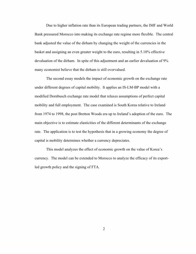
Due to higher inflation rate than its European trading partners, the IMF and World
Bank pressured Morocco into making its exchange rate regime more flexible. The central
bank adjusted the value of the dirham by changing the weight of the currencies in the
basket and assigning an even greater weight to the euro, resulting in 5.18% effective
devaluation of the dirham. In spite of this adjustment and an earlier devaluation of 9%
many economist believe that the dirham is still overvalued.
The second essay models the impact of economic growth on the exchange rate
under different degrees of capital mobility. It applies an IS-LM-BP model with a
modified Dornbusch exchange rate model that relaxes assumptions of perfect capital
mobility and full employment. The case examined is South Korea relative to Ireland
from 1974 to 1998, the post Bretton Woods era up to Ireland’s adoption of the euro. The
main objective is to estimate elasticities of the different determinants of the exchange
rate. The application is to test the hypothesis that in a growing economy the degree of
capital is mobility determines whether a currency depreciates.
This model analyzes the effect of economic growth on the value of Korea’s
currency. The model can be extended to Morocco to analyze the efficacy of its export-
led growth policy and the signing of FTA.
3
CHAPTER 1. THE US – MOROCCO FREE TRADE AGREEMENT: A
GENERAL EQUILIBRIUM ANALYSIS OF IMPLICATIONS FOR MOROCCO
1. Introduction
Since 1995 Morocco has been working closely with the United States to develop a
free trade agreement (FTA) that would allow for stronger economic relations, freer trade,
and better investment conditions between the two countries. Morocco has implemented a
series of adjustments and reforms to facilitate its inclusion into the world economy,
including privatizing public companies, reducing government spending, and reforming
laws and regulations to reduce constraints on entrepreneurial activities and to attract
foreign investment. Morocco’s commitment to the principles of free trade is symbolized
by the passing of the Foreign Trade Law in 1992 that reversed the legal presumption of
import protection. Quantitative restrictions on the import of politically sensitive goods
such as flour and sugar were replaced by tariffs both ad-valorem and variable. In July
2001 a new anti-competition law was passed creating legal sanctions and outlawing anti-
competitive behavior, and establishing an authority to survey market competition.
Morocco’s macroeconomic management has been more successful than in most
other countries in the Middle East and North Africa according to indicators such as the
rate and volatility of inflation, level of the budget deficit, and the stability of the real
exchange rate (Page and Underwood, 1997). In trade, the level and dispersion of tariffs
have been reduced while quantitative restrictions have been eliminated (Alonso-Gamo,
4
Fennell, and Sakr, 1997). Nevertheless in spite of more than two decades of far-reaching
trade reforms, Morocco still has significant trade barriers with a high degree of dispersion
across protection rates.
The US – Morocco FTA implemented in 2005 provides immediate reciprocal
tariff elimination including the immediate elimination of duties on more than 90% of the
value of current bilateral trade in consumer and industrial products. The FTA also
provides bilateral tariff elimination on many agricultural products with most other tariffs
phased out within 15 years. US agricultural producers will benefit from new tariff rate
quotas (TRQs) that provide better access to Morocco. This trade liberalization is likely to
increase the competitiveness of US manufacturers and farmers in Morocco not only
relative to Moroccan producers but also relative to other foreign suppliers such as the
European Union with which Morocco already has an FTA.
The FTA signed with the European Union (EU) commits Morocco to a gradual
removal of its barriers to industrial imports from Europe in exchange for aid, technical
assistance, and a slight improvement in access to the EU market for its agricultural
exports. The EU is Morocco’s major trading partner, representing 75% of exports and
49% of imports (UN Trade Statistics, 2003).
The purpose of the present paper is to estimate the effects of the US – Morocco
FTA on income distribution and on the adjustment of output, factor prices, and
unemployment in different sectors of Morocco’s economy. The present model ties the
change in unemployment to change in income using Okun’s law in its first direct
application in an applied general equilibrium model. The analysis uses a simple
competitive general equilibrium model and covers 34 economic sectors.
5
1.1. Economic Profile
Morocco is strategically located on the northwestern most tip of Africa, across the
straight of Gibraltar only nine miles south of Europe. The World Bank ranks Morocco as
a middle-income developing country with a GDP per capita for 2005, PPP adjusted, of
$4,300. Morocco’s total area is 172,413 square miles, slightly larger than the state of
California. Morocco’s economy measured by GDP is 1.1% of the US GDP, and its
population is 10% of US population. The labor force in Morocco is evenly distributed
between rural areas and urban areas. The service sector is concentrated in urban areas
and represents the largest sector in Morocco’s economy accounting for almost one-half of
GDP. The service sector and employs 45% of the labor force and contributes 42.6% to
GDP with the majority of Morocco’s services exports generated by the travel and tourism
sector. Tourism ranks as the second most important source of foreign currency after
remittances from Moroccans residing abroad. Morocco has approximately three quarters
of the world’s phosphates reserves. It is the world’s leading exporter and third largest
producer of phosphates after the US and Russia.
The agricultural sector contributes 21.7% to GDP but employs 40% of the labor
force (77% rural and 6.3% urban). The agricultural share of labor force attests to the
relatively high labor intensity of agriculture. Agricultural products represent 30% of
exports and 20% of imports. Morocco’s economic growth is closely tied to the
performance of the agricultural sector. The industrial sector employs 15% of the labor
force and contributes 35.7% to GDP. Morocco’s geographic proximity and historical ties
to France and Spain mean that most of Morocco’s economic and trade relations are with
Europe. France, Portugal, and Spain are the largest foreign direct investors in Morocco,
6
combined they accounted for more than 90 % of foreign direct investment in 2001.
Although Morocco’s economy is relatively diversified, agriculture still plays a central
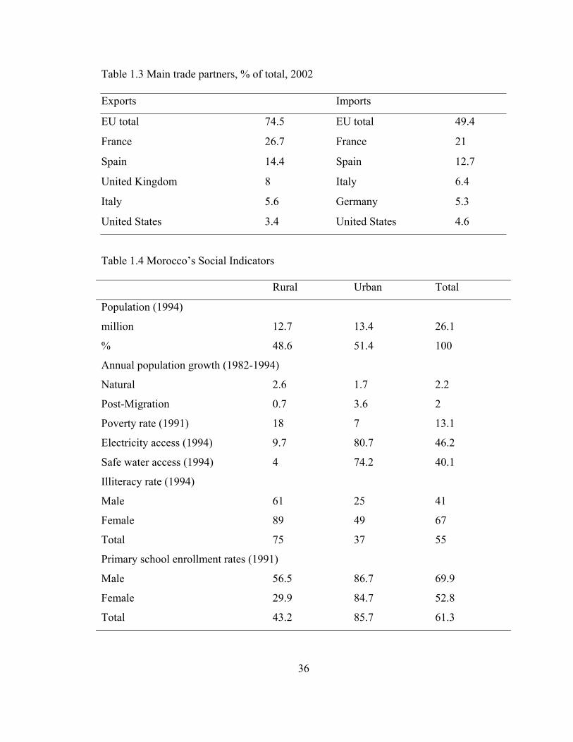
role. Table 1.1, Table 1.2, and Table 1.3 show Morocco’s economic indicators, main
trade commodities, and main trade partners respectively.
1.2. US – Morocco Trade Relations
In 2003, The United States recorded a $66 million trade surplus with Morocco,
4.6% of Morocco’s total imports valued at $462 million came from the US, while 3.4%
of Morocco’s total exports valued at $396 million was shipped to the US. Morocco is the
69th largest market for US exports, and the 82nd largest exporter to the US. Morocco’s
leading exports to the US are transistors, integrated circuits, minerals, calcium
phosphates, and women’s and girls’ garments. Leading US exports to Morocco are
aircraft, soybeans, corn, and wheat. About 60% of shipments from Morocco entered the
United States duty free in 2003 on a normal trade relations (NTR) basis or under
Generalized System of Preferences (GSP) program or other US provisions.
Morocco is a member of the World Trade Organization (WTO) and has tariffs at rates
ranging from zero to 380%.
1.3. US – Morocco Free Trade Agreement
The US – Morocco FTA addresses four important areas: market access, trade
facilitation, investment, and the regulatory environment. Market access refers to the
degree of openness or accessibility that one country’s goods and services experience in
another market and the extent to which one country’s goods and services can compete
with local goods and services in another market. Under the US – Morocco FTA and
relying upon broader commitments both countries have made in the WTO, the two
7
countries agreed to progressively eliminate duties on originating goods and to implement
a wide array of customs procedures that would enhance trade to ensure consistent
customs treatment by both parties (USITC, 2004). The US – Morocco FTA also
stipulates that no new duties would be imposed, that trade restrictions cannot be applied
by either country except in special cases, that administrative fees related to trade would
be limited to the cost of services rendered, and that merchandise processing fees must be
eliminated.
The FTA also establishes a set of obligations in other areas that are more difficult
to quantify such as rules of origin, trade in services, investment, trade facilitation
including customs administration, technical barriers to trade, sanitary and phytosanitary
regulations, electronic commerce, and transparency, and the regulatory environment
including safeguards and trade remedies, government procurement, the protection and
enforcement of intellectual property rights, labor, and the environment.
The agreement is expected to significantly impact sectors and industries undergoing the
greatest degree of tariff liberalization such as machinery and equipment, grains,
processed food, tobacco, petroleum, coal, chemicals, rubber, plastic products, and textiles
and apparel.
With the implementation of FTA, some sectors of the Morocco’s economy are
expected to face increased import competition, resulting in falling prices and output,
while others are expected to profit from rising prices and output as new export
opportunities emerge. The economy of Morocco can be divided into two categories; a
rural economy heavily dependent on agriculture, and a diversified urban economy driven
8
by the service and the industrial sectors. The performance of the agricultural sector
gauges Morocco’s economic growth.
Agriculture employs 77% of the rural labor force and only 6.3% of the urban
labor force. Unemployment in rural areas is low compared to unemployment in urban
areas. In 2004 rural unemployment was 3.2% while urban unemployment was 18.4%.
Although unemployment is low in the country side, the rural population is heavily
disadvantaged according to social and economic indicators. While rural population
makes up half the population of Morocco, it accounts for 70% of the country’s poor.
Table 1.4 shows rural and urban areas access to electricity and safe water, literacy, and
school enrollment. Low educational achievement is reflected in a rural labor force that
for the most part is unskilled. Most jobs in rural areas require no formal education. The
rural-urban skill gap is a major source of income inequality. On average skilled workers
earn 6-7 times the wage of unskilled workers (Karshenas, 1994). One of the
distinguishing features of rural employment that helps explain the low level of
unemployment is the scale of employment in kind which represent 53.9% of rural
employment compared with 6.5% in urban areas according to Löfgren (1999). Rural-
Urban migration is another factor explaining the low level of unemployment in rural
areas. Relatively unfavorable social and economic conditions and chronic drought have
led to rapid rural-urban migration, which provides an important outlet for the rural labor
force absorbing the bulk of its natural growth. The natural growth rate of the population
in rural areas is one and half times higher than that of urban areas 2.6% and 1.7%, but the
overall growth of the population in rural areas is less than 20% that of urban areas 0.7%
9
and 3.6%. The influx of rural population to urban areas exacerbates urban
unemployment and puts downward pressure on urban unskilled wages.
The US – Morocco FTA overall impact on the economies of both countries will
be different. The FTA is expected to affect certain US industries mildly, but the overall
effect on US employment, production and prices is expected to be negligible because of
the small size of Morocco’s economy. In 2004, US imports from Morocco represented
0.04% of total imports while exports to Morocco represented 0.06% of total exports. A
100% increase in trade between the two countries would still be negligible by US
standards. On the other hand, the impact on Morocco’s economy will be significant,
especially on the agricultural sector. The elimination of agricultural protection would
generate significant aggregate welfare gains at the same time a considerable part of the
disadvantaged rural population would lose strongly.
2. The Model
2.1. The General Equilibrium Model of Production and Trade
In the 1970s economists began to develop and use applied general equilibrium
(AGE) models to evaluate the welfare and resource allocation effects of trade and
domestic tax policies. AGE models specify explicit forms of demand and supply
functions that make it possible to solve for the equilibrium values of prices and quantities
once the model is fitted or scaled to a set of data.
The focus of all AGE models is the computation of changes in equilibrium values
of endogenous variables brought about by changes in exogenous policy variables such as
removal of subsidies or imposition of tariffs. The changes in endogenous variables can
be derived using one of two methods. The first method derives the global changes in the
10
model’s endogenous variables while the second derives the local comparative static
changes.
The present emphasis is on general equilibrium comparative statics, and assumes
constant returns, non-joint production, competitive pricing, and cost minimization.
Factors of production are fully employed with the exception of labor. It is an application
of the competitive model of production and trade summarized by Jones and Scheinkman
(1977), Chang (1979), and Thompson (1989, 1995).
2.2. The Specific Factors Model
The Heckscher-Ohlin-Samuleson (H-O-S) theory describes the long run
equilibrium of an economy and assumes that factors of production can costlessly move
across sectors within the economy. Empirical evidence on wage differences and capital
return across industries questions this assumption. Krueger and Summers (1988), Katz
and Summers (1989), and Fels and Grundlach (1990) found that even after adjusting for
differences in worker ability, lasting wage differences remained across industries and for
long periods of time for both the US and Germany. Grossman and Levinsohn (1989) also
found evidence of lasting differences in the return to capital across industries. The labor
force in Morocco is composed of skilled mostly urban labor and unskilled mostly rural
labor. Although empirical evidence has found that labor is relatively immobile across
sectors, in the present paper skilled labor is assumed not to be sector specific but area
specific. For instance, skilled labor is mobile across sectors employing skilled labor
which happens to be concentrated in urban areas. Unskilled labor cannot be employed in
urban sectors since it cannot be substituted for skilled labor. Rural-urban migration does
11
not have a significant effect on skilled wages but contributes to the increase in
unemployment.
The specific factors (SF) model modifies the H-O-S model to allow for factors to
be immobile between industries. The SF distinguishes the degree of factor mobility in
terms of three periods:
The short run period: All factors are perfectly immobile
The medium run period: some factors are mobile while others are immobile
The long run period: all factors are mobile.
An important characteristic of the SF model is that the degree of factor mobility
has an influence on how factor prices and factor incomes respond to change in exogenous
variables.
2.3. The Model
The primary factors of production labor (L), capital (K), and energy (E) are used
in agriculture (A), manufactures (M), and services (S). Thompson (1989) shows the
mechanisms of the model through a geometric illustration. First, standard isoquants
representing unit values of A, M, and S are positioned by their exogenous prices.
Second, cost minimization guarantees that each unit value isoquant is supported by a
common unit isoquant line with endpoints pj/w = 1/w, pj/r =1/r, and pj/e = 1/e (j = A, M,
S). Third, factor inputs are functions of w, r, and e determined at aij (i = L, K, E and j =
A, M, S) where aij is the cost minimizing unit input i in industry j. Production functions
are homothetic and exhibit constant returns, implying that each expansion path is linear at
a given input price ratio.
12
The endowment of factors of production L, K, and E are given. With all available
factors employed, outputs of A, M, and S are determined. If labor is not fully employed
and employment N depends on income then output would be biased towards capital
intensive manufactures. With income rising, the ratio of labor-intensive services and
agriculture to manufactures increases. Production would then move along the
Rybczynski line as the production possibilities frontier expands.
Okun’s law is a noted empirical relationship between the change in
unemployment rate and the percentage change in national income. Using Okun’s law as
in Thompson (1989) let u represent the unemployment rate:
u = (L – N)/L u > 0 (1)
Changes in unemployment and changes in the level of national income are assumed to be
linearly related,
du = αdY α > 0 (2)
Differentiating (1) du = (NdL – LdN)/L2 and substituting into (2)
dN = (1 – u)dL + αdY (3)
Equation (3) becomes part of the general equilibrium model showing that
employment N is related to the exogenous endowment of labor and the endogenous
national income.
Employment is written as
N = aLAxA + aLMxM + aLSxS (4)
where xj represents output (j = A, M, S). Differentiating (4) and using (3) gives
(1 – u)dL + αdY = ΣjaLjdxj + sLLdw + sLKdr + sLEde (5)
13
The aggregate economy substitution terms sik (i,k = L, K, E) summarize how
firms alter their input mix when factor payments change, sik = Σjxjaih
j where aih
j =
daij/dwh. By Shepard’s lemma and Taylor’s formula, sik = ski. If sik is positive (negative),
factors i and k are aggregate substitutes (complements).
Full employment in capital yield a simpler relationship,
dK = ΣjaKjdxj + sKLdw + sKKdr + sKEde (6)
Similarly for energy,
dE = ΣjaEjdxj + sELdw + sEKdr + sEEde (7)
Competitive pricing of each good implies
pj = Σiwiaij (8)
Differentiating (8) gives three more equations for the model
dpj = aLjdw + aKjdr + aEjde j = A, M, S (9)
given the cost minimization envelop result, wdaLj + rdaKj + edaEj = 0.
National income is the sum of the payment to each factor of production
Y = wN + rK + eE (10)
Differentiating (10) and using (3) gives the final equation for the model
γdY – Ndw – Kdr - Ede = (1 – u)wdL + rdK + edE (11)
where γ = (1 – αwL).
Organizing (2) and (5) through (11) in matrix form with the exogenous variables
on the right,
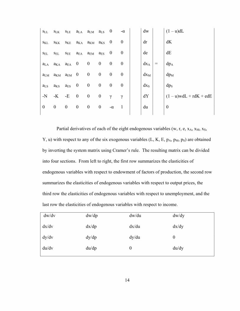
14
sLL sLK sLE aLA aLM aLS 0 -α dw (1 – u)dL
sKL sKK sKE aKA aKM aKS 0 0 dr dK
sEL sEL sEE aEA aEM aES 0 0 de dE
aLA aKA aEA 0 0 0 0 0 dxA = dpA
aLM aKM aEM 0 0 0 0 0 dxM dpM
aLS aKS aES 0 0 0 0 0 dxS dpS
-N -K -E 0 0 0 γ γ dY (1 – u)wdL + rdK + edE
0 0 0 0 0 0 -α 1 du 0
Partial derivatives of each of the eight endogenous variables (w, r, e, xA, xM, xS,
Y, u) with respect to any of the six exogenous variables (L, K, E, pA, pM, pS) are obtained
by inverting the system matrix using Cramer’s rule. The resulting matrix can be divided
into four sections. From left to right, the first row summarizes the elasticities of
endogenous variables with respect to endowment of factors of production, the second row
summarizes the elasticities of endogenous variables with respect to output prices, the
third row the elasticities of endogenous variables with respect to unemployment, and the
last row the elasticities of endogenous variables with respect to income.
dw/dv dw/dp dw/du dw/dy
dx/dv dx/dp dx/du dx/dy
dy/dv dy/dp dy/du 0
du/dv du/dp 0 du/dy
15
Each row can be used to simulate the effect of changes in exogenous variables on
endogenous variable. For instance, to simulate the effects of tariff removal on
endogenous variables (w, r, xA, xM, xS, Y, u), row two is multiplied by a vector of the
expected price changes resulting from the tariff removal.
3. The Data
3.1. Morocco Factor Shares and Industry Shares
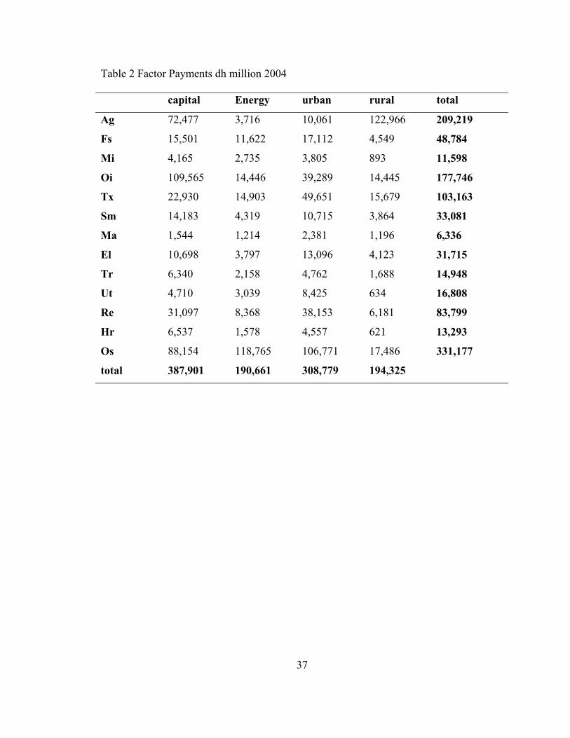
The first step in applying specific factor model is to compute the factor share
matrix θ and industry share matrix λ. Table 2 is the total payment matrix used to derive
factor shares and industry shares.
Factor shares are the portions each productive factor receives from industry
revenue, and industry shares are the portions of productive factors employed in each
industry. There are thirteen sectors and four productive factors. Capital is assumed
sector specific, while labor is divided into two groups, urban employed mostly in the
service and industrial sector, and rural labor employed mostly in agriculture. Energy is
the only factor shared by all sectors and areas.
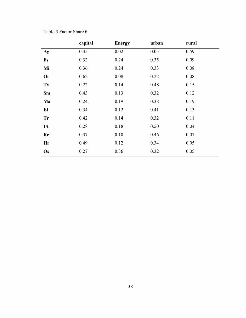
Summing across a row in Table 2 gives sector value added. Table 3 summarizes
factor shares. Value added in agriculture is Dh209.21 billion (Dirham Dh, $1 = 9Dh) and
the rural labor share is 122.96/209.21 = 58.8%, the energy share is 1.8%, and the capital
share is 34.6%. The manufacturing sector is capital intensive using the share measure,
with capital share varying dramatically from one sector to another. The factor share of
capital in other industries is 61.6% while factor share of urban labor is 22.1%, and rural
labor is 8.1%
16
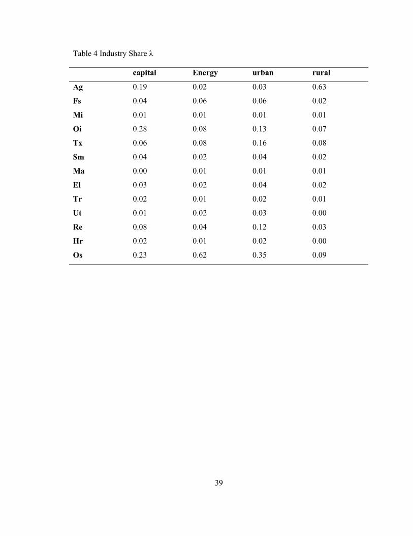
Industry shares in Table 4 summarize the distribution of inputs across industries.
Summing down a column in Table 2 gives total factor incomes. For example, total
income of urban labor in all sectors is Dh308.77 billion. The industry share of
agricultural rural labor is 63.6%. The industry share of capital in other industries is
28.2%, the largest industry share of capital. Capital is sector specific with each capital
industry share 1 in its own industry.
3.2. Morocco Static Elasticities
Substitution elasticities as developed by Jones (1965) and Takayama (1982)
summarize cost minimizing inputs adjustment when factor prices change. Following
Allen (1938), the cross price elasticity between the input of factor i and the payment to
factor k in sector j is
Eik
j = âij/ŵk = θkjSih
j (12)
where Sih
j is the Allen partial elasticity of substitution. Cobb-Douglas production implies
Sih
j = 1. With constant elasticity of substitution (CES) production, the Allen elasticity
can have any positive value. Given linear homogeneity, ΣkEik
j = 0 and the own price
elasticity Eiij are the negative sum of cross price elasticities.
Substitution elasticities are the weighted average of cross price elasticities for
each sector
σik = â/ŵk = ΣjλijEik
j = ΣjλijθkjSih
j (13)
Factor shares and industry shares are used to derive the Cobb-Douglas
substitution elasticities in Table 5. With Cobb-Douglas or CES the rule is substitution
between inputs.
17
The largest own price elasticity is for energy and the smallest is for capital in
other industries. Every 10% increase in the energy price causes a 17.6% decline in
energy usage, and every 10% increase in the return to capital decreases its input in other
industries by 3.84%. Constant elasticity of substitution would scale the elasticities in
Table 5. When CES = 0.5, elasticities would be half as large as those in Table 5.
The comparative static elasticities of the system are in the inverse of the system
matrix in (13) and are derived using Cramer’s rule. Table 6 shows elasticities of factor
prices with respect to prices of goods and services in the general equilibrium. The effects
of price changes on factor payments are uneven in that with any price change some
factors benefit and others lose.
The focus is on adjustments to the likely range of price changes due to the
removal of trade barriers. Morocco’s base tariff rates usually reach 50% ad valorem and
in some cases related to TRQ products and other sensitive agricultural imports reach up
to over 300%. Under the FTA agreement, Morocco would eliminate duties on many U.S.
exports immediately while phasing out duties on some U.S. agricultural goods including
TRQ categories and more sensitive industrial products over periods of 2 to 25 years.
The US average tariff rate on imports from Morocco is around 4% ad valorem, a
relatively low rate. The average tariff rate for U.S. goods entering Morocco is in excess
of 20%. It is expected that the sectors that have had relatively higher trade protection
will show larger effects from the implementation of the FTA. Agricultural prices are
expected to fall as trade barriers are eliminated and domestic producers face increasing
competition from US agricultural products, especially wheat which has been highly
18
protected. According to the USDA, during 1998-2003 the average Moroccan duty was
17.5% on corn, 28.4% on durum wheat, and 83.3% on bread wheat.
Table 6 shows that every 10% decrease in agricultural prices would lower
agricultural rural wages and payment to capital in agriculture by 2.89% and 23.8%, and
increase urban agricultural wages by 0.51%, a significant impact for capital (land) owners
and rural agricultural labor. Some industrial sectors are also expected to suffer from
increased competition with US products. The biggest effect on the return to capital will
be in machinery sector, a relatively small sector in Morocco. Every 10% decrease in
price of machinery will lower the return to capital and wages by 40.7% and 1% for urban
workers. Labor in machinery is considered skilled labor and will not be affected
significantly by a decrease in machinery prices since it can move to other expanding
urban sectors. The expected winners from FTA are export sectors and services. One of
the sectors expected to benefit from FTA is the fishing industry.
Morocco's coast line covers 2,141 miles along the Mediterranean Sea and Atlantic
Ocean. The ocean off Morocco's Atlantic coast is one of the richest fishing grounds in
the world. Since the 1930s, fishing has been a major industry in Morocco and its
importance to the economy grew as the industry matured. The industry experienced
tremendous growth and revamping during the 1980s, and since 1983 the annual catch has
exceeded 430,000 tons. In 1986 and 1991 landings were the largest ever, exceeding
594,000 tons. In 1990, exports of fish and fish products were equivalent to 8% of total
exports. Today, these exports account for approximately 45% of agricultural exports and
employ over 100,000 people. The industry's importance is underscored in both the
employment sector and by the $600 million plus of foreign exchange that the industry
19
brings in each year. Every 10% price increase will increase return to capital in the
fishing industry by 30.3%, but will not significantly raise wages in the industry.
The mining sector is also expected to gain from FTA. Morocco’s mining sector is
dominated by the mining of phosphates. Morocco has 76% of the world phosphates, and
is the largest exporter and third largest producer after the US and Russia. Morocco’s
other mining industries include iron ore, manganese, lead, and zinc. A 10% price
increase in the mining sector will raise return to capital by 27.7% but will have negligible
effect on wages. The service sector is also expected to gain from FTA, with return to
capital in the service sector benefiting the most, return to capital in construction and real
estate related services is will increase by 25.7%, the return to capital in the hospitality
industry will increase by 20.3%, and in other services by 23.5%. The impact on wages
will be minimal with the exception of wages of urban workers in other services where a
10% price increase will lead to a 6.6% increase in their wages.
The comparative static effects of price changes on factor prices are the same for
all CES production functions. Comparative static elasticities in Table 6 extend to all CES
production functions regardless of substitution.
Price elasticities of output along the production possibility frontier are
summarized in Table 7. A higher price raises output in a sector, attracting labor and
energy from other sectors and lowering output in other sectors. Energy is a shared factor
and will move without cost across sectors and areas. Labor in urban areas will move
across sectors from the contracting to the expanding industries, but will not move to rural
areas. Capital is sector specific and will not move.
20
Output in agriculture is expected to decrease as agricultural prices fall. Table 7
shows that a 10% price decrease in the price of agriculture will cause a 13.8% decrease in
output.
Morocco is an important producer, consumer, and importer of barley and of
durum and bread wheat. Grains are important staples in the Moroccan diet. The
Moroccan government provides price support for wheat sold to licensed agents, and a
retail wheat flour subsidy for low income consumers covering about 1 million metric ton
(mt) of bread flour, about one-sixth of domestic wheat consumption. Morocco’s corn
production is insignificant. USDA states that there were about 1.5 million farmers in
Morocco who grew wheat and barley in 2003. Moroccan farmers grew 1.0 million mt of
durum wheat, 1.9 million mt of bread wheat, and 1.3 million mt of barley annually during
the period 1998-2002.
Because Moroccan grain production is rain fed and is periodically subject to
drought conditions, output is extremely variable from year to year. Moroccan crop yields
fell by more than 10 percent in 6 of the 10 years during 1991-2000.
According to the USDA, during 1999/2000 to 2002/03 Morocco’s average annual import
of wheat was 3 million mt, approximately one-half of Morocco domestic consumption.
Average annual import of coarse grains including corn was 1.4 million mt also about one-
half of domestic consumption. Shapouri and Rosen (2003) projected that Moroccan
imports of all grains are will grow annually by nearly 1 million mt during 2002-2012 to
maintain the current level of per capita consumption.
In the industrial sector, output of machinery is expected to decrease. A price
increase of 10% will lower output by 30.73%. The fishing industry will increase output
21
by 20.34% following a 10% price increase. Mining output will increase by 17.66%, other
industries by 5.86%. Textile, garment and furs, and leather and shoes will increase by
28.71%. The textile, garment and furs, and leather and shoes are important sectors in
terms of the size of the labor force employed and the contribution to GDP. Hotel and
restaurant services are expected to increase by 10.26% following a 10% price increase, a
relatively modest adjustment. Travel and Tourism is a well developed sector in the
economy and ranks as the second largest foreign currency earner. The modest adjustment
may be due to the fact that tourism sector in Morocco is relatively efficient and operates
at close to full capacity. Tourism also faces competition from neighboring countries
especially Spain and Tunisia.
Between 2003 and 2004 the number of unemployed declined by 2.45% or 30,000
people and total income increased by 5.77% or Dh45.89 billion. Okun’s law relates the
change in unemployment rate to the percentage change in national income. Using
Okun’s law as shown by Thompson (1989) the rate of change in unemployment assumed
to be linearly related to income can be derived using (2). The rate of change in
unemployment due to rising income represented by α is 0.425 where α represents the
elasticity of unemployment with respect to income. An increase in income of 10%
lowers unemployment by approximately 4.25%.
Various studies have estimated the economic impact of the US-Morocco FTA on
the both countries. Gilbert (1999) predicts that the effects on the US economy would be
negligible, 0.04 increase in imports, 0.03 % increase in exports, and no change in GDP.
The effects of FTA on Morocco would be significant because of the relatively small size
of Morocco. Brown, Kiyota, and Stern (2004) estimated a $920 million or 2.08% welfare
22
gain for Morocco. FTA benefits primarily will accrue to the export sector and the
tourism industry, and will exacerbate problems in the agricultural sector. Using the
Brown, Kiyota, and Stern (2004) estimate, unemployment is projected to decrease by
1.19%. Most of the new jobs created by FTA will be skilled jobs located in urban areas.
Since the two labor markets are insulated from each other, unskilled mostly rural labor is
not a substitute for skilled mostly urban labor, and the gain will accrue mostly to skilled
labor and not trickle down to rural labor. The gain in terms of wages may be modest.
Rural labor will see its wages further depressed and the FTA will be the impetus for the
acceleration of rural-urban migration. The gain in terms of jobs created will be offset by
the rural-urban migration that will swell the ranks of the unskilled unemployed. The
overall effect of FTA on job creation may be negative at least in the immediate term
before workers can relocate and retrain.
3.3. Projected Adjustment with FTA
Morocco maintains high tariff barriers relative to the US. The FTA will make the
products of each country more accessible and more competitive in each other’s market.
Gilbert (2003) estimates the US-Morocco FTA would increase imports from Morocco to
the US by 18.20 %, and US exports to Morocco by 88.25 %. Tariffs on grains range
from 17.5 % for corn to 83.3 % for bread wheat. The removal of tariffs would make US
agricultural products more competitive and would enable the US to regain its position as
the major supplier of corn to Morocco, as well as gain a larger market share of other
grains.
23
Based on the literature we expect agricultural prices to fall by 5% to 15%, mining
prices to increase by 5%, machinery prices to fall 5%, and prices in the service sector to
increase 5%. Table 8 summarizes the expected changes in prices.
To find the endogenous vector of factor price adjustments, multiply a vector of
predicted price changes by the matrix of factor price elasticities in Table 6. Table 9 uses
the expected price changes in Table 8. Results scale to the level of price changes, 10%
price changes double the adjustments. The energy price is exogenous at the world level.
Urban wages increase by 6.1% while rural wages decrease by 1.6%. The largest decrease
in return to capital is in agriculture 41.2%, followed by machineries at 26.6%, steel and
metal-work 3.4%, automobiles and other transportations 3.2%, and other industries 1.6%.
The largest increase in return to capital is in other services increases by 15.3%, followed
by textiles, garments and furs, and leather approximately 12.1%, fishing industry 11.5%,
mining 10.5%, electrical equipment and electronics 8.9%, utilities, 8.9%, construction
and real estate 7%, and hotel and restaurant 6.7%.
The endogenous vector of output adjustments is found by multiplying the vector
of predicted price changes in Table 8 by the matrix of output price elasticities in Table 7.
Sectors where return to capital is expected to decrease will also see a decrease in output.
Agricultural output at 26.3%, followed by machinery output will fall by 21.6%, steel and
metal-work 3.4%, automobiles and other transportations 3.2%, and other industries 1.6%.
The highest increase in output will be in the other services 10.3%, followed by textiles,
garments and furs, and leather approximately 7.1%, fishing industry 6.5%, mining
approximately 5.5%, electrical equipment and electronics 3.9%, utilities3.9%,
construction and real estate 2%, and hotel and restaurant less than 1.7%.
24
The output adjustments are modest relative to change in return to capital. The
change in the return to capital will affect investment, generating larger long-run output
adjustments. Assume a unit elasticity capital stock with respect to its return. In the
present model, the percentage long-run adjustment in output is equal to the percentage
change in the industry’s capital stock. These long-run output adjustments are in the last
column of Table 9. Output will further decline in the contracting industries and increase
in expanding industries as the economy becomes more specialized. Agricultural output
will decline by 41.2%, while fishing and mining outputs will increase by 11.5% and
10.5%.
The percentage change in machinery output is almost twice that of agriculture, but
its impact will be relatively insignificant. FTA is expected to lower income by 0.04%
and increase unemployment by 0.02%. The increase in unemployment will affect rural
areas primarily.
The specific factors model provides insight into the potential output adjustments
and income redistribution in Morocco under the FTA with the US as markets adjusts and
the economy moves along its production frontier toward a new production pattern.
Morocco’s agriculture will suffer falling prices and import competition.
Sectors that are expected to benefit from FTA use unskilled labor less intensively than
skilled labor, and may not be able to absorb the displaced unskilled rural labor. Chronic
drought and unfavorable rural conditions accentuated by FTA will lead to rapid rural-
urban migration, which provides an important outlet for the rural labor force absorbing
the bulk of its natural growth but exacerbates urban unemployment and depresses urban
unskilled wages.
25
FTA will have a greater impact on rural areas where labor is concentrated in
agriculture. According to data from the early 1990s, per-capita consumption in rural
areas is about half the consumption in urban areas. Rural areas also account for 70 % of
Morocco’s poor. The gains from FTA which are expected to go mostly to urban areas
and urban skilled labor will be offset by the losses in rural areas. The present model uses
Okun’s law in its first application in an applied general equilibrium model to tie the
change in unemployment to change in income.
Morocco’s attempts at decentralizing industrial activity and promoting industrial
investments in rural areas have been modestly successful. Most of the service and
industrial activities are concentrated in Casablanca. Casablanca is considered the
economic capital of Morocco. With the largest population and the biggest port it is the
biggest city in Morocco. Casablanca’s port complex has become the city's economic
centre, and is one of the largest artificial ports in the world covering an area of 445 acres.
The port is the second largest in North-Africa, handling around 70% of Morocco's
shipping.
To end the isolation of rural areas, Morocco launched in 1995 the National Road
Construction Program (PNCRR) designed to decentralize the economy by building a
network of toll freeways that will link the country’s interior to the coastal cities and ports.
Over a nine-year period, an additional 10,000 km of rural roads were built. The ongoing
program will link the Casablanca-Rabat highway to the other major cities. The Rabat-
Tangiers highway is 225 km and connects the capital to the north and runs along the
Atlantic coast, Rabat-Fez highway is 180 km long and runs west to east connecting the
capital to the heartland, Casablanca-Taroudant highway is 555 km and runs north to south
26
along the atlantic coast. In addition a Mediterranean by-pass 530 km long will run west
to east connecting Tangiers to the resort town of Saidia along the Algerian border.
The adoption of the toll system as tool of financing contributed to the establishment of
the freeway program. This financing policy materialized when the Société Nationale des
Autoroutes du Maroc (ADM) was created. ADM’s principal tasks is building, managing
and maintaining the highways network granted to it by the government. The toll system
is designed to remunerate and amortize capital invested by the ADM for both of
construction and management of the freeways. The initial duration of the conceded
freeways was 35 years, later extended to 50 years so as to ensure the recovery of the
capital expenditures. The principal reason for the duration extension is the low level of
traffic in the freeways and the subsequent low revenue. The high tolls have deterred
drivers from using the new freeways. For instance, to drive from Casablanca to Tangiers
a driver must pay dh80 ($8.80) in tolls, first, dh20 ($2.20) for the 100km (60 miles)
linking Casablanca to Rabat, then dh60 ($6.60) for the next 250km (148miles) between
Rabat and Tangiers. ADM is also authorized to set up and operate or lease commercial
facilities such as gas stations, restaurants, hotels, and transport services, within the
geographic vicinity of the highway but it has not yet made use of such an option.
4. Policy Discussion
Since the accession of King Mohammed VI, important steps have been taken to
reform Morocco's economy and to deepen its democratic structures. These steps include
updating Morocco's intellectual property rights legislation, developing a specialized
commercial court system, liberalizing the telecommunications market, and emphasizing
government transparency. All of the government procurement contracts are large
27
projects for which the competition is predominantly European companies. Many of these
projects are financed by multilateral development banks, which impose their own
nondiscriminatory procurement regulations. US companies sometimes have difficulty
with the requirement that bids for government procurement be in French.
The central bank sets the exchange rate for the dirham against a basket of
currencies of its principal trading partners, particularly the euro that is given a strong
weight and the currencies of the European trading area. This exchange rate mechanism
causes dollar to dirham exchange rate to be highly volatile. This volatility increases the
foreign exchange risk of importing from the United States as compared to importing from
Europe.
The Moroccan dirham is convertible for all current transactions, as well as for
some capital transactions, especially capital repatriation by foreign investors. The
Moroccan dirham is available through commercial banks for such transactions upon
presentation of documents. Moroccan companies are permitted to borrow abroad without
prior government approval. Moroccan individuals or corporations investing abroad must
seek approval from the Foreign Exchange Board. The use of international credit cards by
Moroccans is severely restricted, making it nearly impossible to use e-commerce to
purchase goods internationally.
Due to a higher inflation rate than its European trading partners, the IMF and
World Bank pressured Morocco into making its exchange rate regime more flexible. The
central bank adjusted the value of the dirham by changing the weight of the currencies in
the basket and assigning an even greater weight to the euro, resulting in 5.18% effective
28
devaluation of the dirham. In spite of this adjustment and an earlier devaluation of 9%
many economist believe that the dirham is still overvalued.
In November, 1989, parliament abolished a 1973 law requiring majority
Moroccan ownership of firms in a wide range of industries. This law served as a barrier
to US investments in Morocco. In 1993, the Moroccan government eliminated a 1974
decree restricting foreign ownership in the petroleum refining and distribution sector, and
allowed Mobil Oil to buy back the government's 50% share of Mobil's Moroccan
subsidiary in 1994.
Morocco sees foreign investment as a key to development and is doing everything
it can to attract investors and improve its infrastructure for trade. For example, Morocco
is becoming a popular base for French call centers, with the state rail company, SNCF,
and France Télécom among the early operators there. US companies have a small but
growing presence in Morocco. Dell Computer operates a 24-hour call center, and
Motorola has some assembly operations. Several US trade associations such as
ConnectUS, which includes Google and Cisco Systems among its members, and the
Morocco-American Trade and Investment Council, which includes Dell and Oracle
Corporation as members, are also actively promoting commerce with Morocco.
Despite relatively strong macroeconomic indicators, low inflation levels (approximately
2%), and foreign currency reserves providing approximately six months of import
coverage, persistent structural problems still hinder Morocco’s economy. Over the last
decade economic growth has been weak, partly because of dependence on agriculture –
the primary motor of economic growth, and sporadic but recurring drought. A two-year
drought led the economy to contract by 0.7% in 1999 and to grow by only 0.3% in 2000.
29
The effects were felt strongly by the rural population whose living conditions have
deteriorated.
Despite the progress made by the government on economic reform, there is
frequent criticism that the government is not moving quickly enough. The short term
effects of FTA may be severe, especially for agriculture, the most heavily protected
sector and the sector that provides the lion share of income in rural areas. Examples of
short run policies that can be adopted are income transfer programs for rural agricultural
labor, and the elimination of freeway tolls.
An income transfer program similar to Mexico’s PROCAMPO, where farmers are
compensated for the loss of protection of agricultural markets can attenuate the short run
impact of FTA. Transfer payments can be made proportional to past earnings in
agriculture, and specifically designed so as not to distort current production decisions
(World Bank, 1997). The short term income transfer can be supplemented by long term
investments in education and training of rural labor force to help it adapt to the changing
economy conditions, and investments in infrastructure that would facilitate the
development of non-agricultural activities in rural areas.
Eliminating tolls and replacing the financing system of freeways by granting
franchises for commercial activities, such as gas stations, restaurants, and hotels along the
freeway through competitive bidding, would help in promoting industrial development in
the country’s interior. The present financing system is less than adequate. Tolls are set
too high to stimulate high traffic, and are a deterrent to drivers who prefer free secondary
roads. The low traffic does not generate enough revenue to justify additional investments
in commercial ventures along the freeway. Even by wealthy developed countries
30
standards the tolls are too high. For instance, a 148 miles trip from Rabat to Tangiers
costs $6.60 while a 100 miles trip on I-95 in Maine from York to Augusta costs $3.25 in
tolls. According to the World Bank, 2005 income per capita in Morocco is $1520.
Relative to income, highway tolls in Morocco are exorbitant and are the reason they are
deserted. Businesses operating in Morocco’s interior have to consider the cost of using
freeways to access Casablanca’s port and markets. Although they are toll-free, secondary
roads in Morocco are some of the deadliest in the world. International Road Safety News
reports that the toll of dead and injured from road accidents in Morocco is over 3,800 and
15,000 and costs the State 2.5% of the GDP or about $1.2 billion a year.
The SF model does not separate the effect of FTA on rural and urban areas.
Intuitively an increase in income should lead to a decrease in unemployment, as income
rises and the economy grows new jobs are created but a closer look at the effect of FTA
on Morocco’s economy may reveal a different picture. Gilbert (2003) estimates the US-
Morocco FTA would increase imports from Morocco to the US by 18.2 %, and US
exports to Morocco by 88.3 %. The removal of tariffs would make US agricultural
products more competitive, and would enable the US to regain its position as the major
supplier of corn to Morocco, as well as gain a larger market share of other grains. The
agricultural sector in Morocco is labor intensive. Table 10 shows that in 1994-1995
agriculture employed 44.8% of the population, more than half the people employed in
agriculture are paid in kind.
Karshenas estimates that skilled labor earns 6 to 7 times more than unskilled
workers. Most of the unskilled labor is concentrated in rural areas where unemployment
is very low in spite of the huge rural-urban income inequality. Rural agricultural income
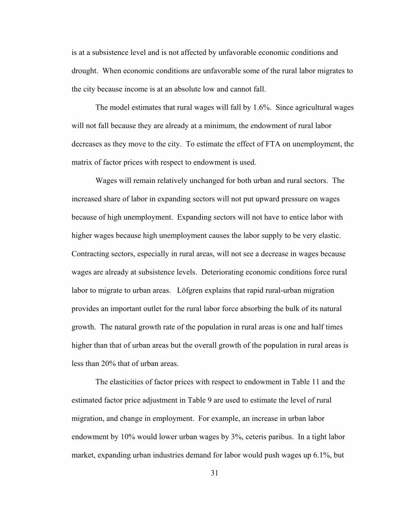
31
is at a subsistence level and is not affected by unfavorable economic conditions and
drought. When economic conditions are unfavorable some of the rural labor migrates to
the city because income is at an absolute low and cannot fall.
The model estimates that rural wages will fall by 1.6%. Since agricultural wages
will not fall because they are already at a minimum, the endowment of rural labor
decreases as they move to the city. To estimate the effect of FTA on unemployment, the
matrix of factor prices with respect to endowment is used.
Wages will remain relatively unchanged for both urban and rural sectors. The
increased share of labor in expanding sectors will not put upward pressure on wages
because of high unemployment. Expanding sectors will not have to entice labor with
higher wages because high unemployment causes the labor supply to be very elastic.
Contracting sectors, especially in rural areas, will not see a decrease in wages because
wages are already at subsistence levels. Deteriorating economic conditions force rural
labor to migrate to urban areas. Löfgren explains that rapid rural-urban migration
provides an important outlet for the rural labor force absorbing the bulk of its natural
growth. The natural growth rate of the population in rural areas is one and half times
higher than that of urban areas but the overall growth of the population in rural areas is
less than 20% that of urban areas.
The elasticities of factor prices with respect to endowment in Table 11 and the
estimated factor price adjustment in Table 9 are used to estimate the level of rural
migration, and change in employment. For example, an increase in urban labor
endowment by 10% would lower urban wages by 3%, ceteris paribus. In a tight labor
market, expanding urban industries demand for labor would push wages up 6.1%, but
32
high unemployment would allow urban industries to increase their demand for labor
without putting upward pressure on wages. To estimate the increase in employment in an
expanding sector, the estimated change in factor prices from Table 9 is combined with
the elasticity of factor prices with respect to endowment.
Employment in agriculture will decrease by 7.7%, while employment in fisheries
and mining will increase by 1.7% and 1.9%. Some of the unemployed in agriculture will
find work in fisheries and mining, but their number is minimal because agriculture dwarfs
the other two sectors.
Table 12 summarizes the change in employment. Expanding sectors will increase
the size of their labor, while contracting sectors will decrease the size of their labor force.
These changes will not affect wages because of high unemployment.
Falling agricultural prices and import competition will accentuate the rural-urban
migration, and keep wages in rural areas relatively stable. In urban areas, the effects of
FTA on wages will depend on workers skill level and their industry. The service sector
will be the net winner, with other services benefiting the most.
5. Conclusion
The US – Morocco FTA provides bilateral tariff elimination on many agricultural
products with most other tariffs phased out within 15 years. US agricultural producers
especially grains producers will benefit from new TRQ that provide better access to
Morocco. The FTA will most likely increase the competitiveness of US manufacturers
and farmers in Morocco not only relative to Moroccan producers but also relative to other
foreign suppliers such as the European Union with which Morocco already has an FTA.

33
The US – Morocco FTA will benefit export industries in Morocco. Employment in
expanding export sectors such as tourism, fisheries, and mining as well as some service
sectors will increase. Import competing sectors will suffer from increased competition
and falling prices. Income for both expanding and contracting sectors will most likely
not change due to Morocco’s high unemployment. The agricultural sector will be the
most severely affected by FTA. The agricultural sector employs 45% of the country’s
labor force and more than two thirds of the rural labor force. Rural areas are
characterized by low unemployment and high levels of poverty. The low level of
unemployment in rural areas is due to rural-urban migration and to the scale of
employment in kind, which represent 54% of rural employment. Relatively unfavorable
social and economic conditions and chronic drought have led to rapid rural-urban
migration, which provides an important outlet for the rural labor force. Wages in rural
areas are at subsistence levels and do not fall when economic conditions worsen. The
FTA will accelerate the rural-urban migration. A small fraction of the displaced rural
laborer will find employment in the expanding mining and fishing sectors, while the
majority will swell the ranks of the unemployed in urban areas, putting more strains on an
already stressed social and economic system.
In future research, I will use a more comprehensive computable general
equilibrium model and disaggregate the sectors into skilled-urban, unskilled urban,
skilled-rural, and unskilled rural sectors.
34
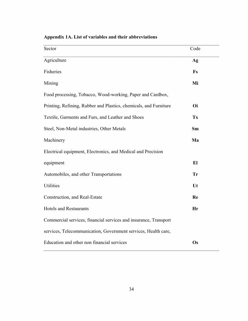
Appendix 1A. List of variables and their abbreviations
Sector Code
Agriculture Ag
Fisheries Fs
Mining Mi
Food processing, Tobacco, Wood-working, Paper and Cardbox,
Printing, Refining, Rubber and Plastics, chemicals, and Furniture Oi
Textile, Garments and Furs, and Leather and Shoes Tx
Steel, Non-Metal industries, Other Metals Sm
Machinery Ma
Electrical equipment, Electronics, and Medical and Precision
equipment El
Automobiles, and other Transportations Tr
Utilities Ut
Construction, and Real-Estate Re
Hotels and Restaurants Hr
Commercial services, financial services and insurance, Transport
services, Telecommunication, Government services, Health care,
Education and other non financial services Os
35
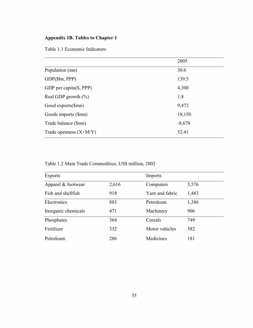
Appendix 1B. Tables to Chapter 1
Table 1.1 Economic Indicators
2005
Population (mn) 30.6
GDP($bn, PPP) 139.5
GDP per capita($, PPP) 4,300
Real GDP growth (%) 1.8
Good exports($mn) 9,472
Goods imports ($mn) 18,150
Trade balance ($mn) -8,678
Trade openness (X+M/Y) 52.41
Table 1.2 Main Trade Commodities, US$ million, 2002
Exports Imports
Apparel & footwear 2,616 Computers 3,576
Fish and shellfish 918 Yarn and fabric 1,483
Electronics 883 Petroleum 1,386
Inorganic chemicals 471 Machinery 906
Phosphates 364 Cereals 749
Fertilizer 332 Motor vehicles 582
Petroleum 286 Medicines 181
36
Table 1.3 Main trade partners, % of total, 2002
Exports Imports
EU total 74.5 EU total 49.4
France 26.7 France 21
Spain 14.4 Spain 12.7
United Kingdom 8 Italy 6.4
Italy 5.6 Germany 5.3
United States 3.4 United States 4.6
Table 1.4 Morocco’s Social Indicators
Rural Urban Total
Population (1994)
million 12.7 13.4 26.1
% 48.6 51.4 100
Annual population growth (1982-1994)
Natural 2.6 1.7 2.2
Post-Migration 0.7 3.6 2
Poverty rate (1991) 18 7 13.1
Electricity access (1994) 9.7 80.7 46.2
Safe water access (1994) 4 74.2 40.1
Illiteracy rate (1994)
Male 61 25 41
Female 89 49 67
Total 75 37 55
Primary school enrollment rates (1991)
Male 56.5 86.7 69.9
Female 29.9 84.7 52.8
Total 43.2 85.7 61.3
37
Table 2 Factor Payments dh million 2004
capital Energy urban rural total
Ag 72,477 3,716 10,061 122,966 209,219
Fs 15,501 11,622 17,112 4,549 48,784
Mi 4,165 2,735 3,805 893 11,598
Oi 109,565 14,446 39,289 14,445 177,746
Tx 22,930 14,903 49,651 15,679 103,163
Sm 14,183 4,319 10,715 3,864 33,081
Ma 1,544 1,214 2,381 1,196 6,336
El 10,698 3,797 13,096 4,123 31,715
Tr 6,340 2,158 4,762 1,688 14,948
Ut 4,710 3,039 8,425 634 16,808
Re 31,097 8,368 38,153 6,181 83,799
Hr 6,537 1,578 4,557 621 13,293
Os 88,154 118,765 106,771 17,486 331,177
total 387,901 190,661 308,779 194,325
38
Table 3 Factor Share θ
capital Energy urban rural
Ag 0.35 0.02 0.05 0.59
Fs 0.32 0.24 0.35 0.09
Mi 0.36 0.24 0.33 0.08
Oi 0.62 0.08 0.22 0.08
Tx 0.22 0.14 0.48 0.15
Sm 0.43 0.13 0.32 0.12
Ma 0.24 0.19 0.38 0.19
El 0.34 0.12 0.41 0.13
Tr 0.42 0.14 0.32 0.11
Ut 0.28 0.18 0.50 0.04
Re 0.37 0.10 0.46 0.07
Hr 0.49 0.12 0.34 0.05
Os 0.27 0.36 0.32 0.05
39
Table 4 Industry Share λ
capital Energy urban rural
Ag 0.19 0.02 0.03 0.63
Fs 0.04 0.06 0.06 0.02
Mi 0.01 0.01 0.01 0.01
Oi 0.28 0.08 0.13 0.07
Tx 0.06 0.08 0.16 0.08
Sm 0.04 0.02 0.04 0.02
Ma 0.00 0.01 0.01 0.01
El 0.03 0.02 0.04 0.02
Tr 0.02 0.01 0.02 0.01
Ut 0.01 0.02 0.03 0.00
Re 0.08 0.04 0.12 0.03
Hr 0.02 0.01 0.02 0.00
Os 0.23 0.62 0.35 0.09
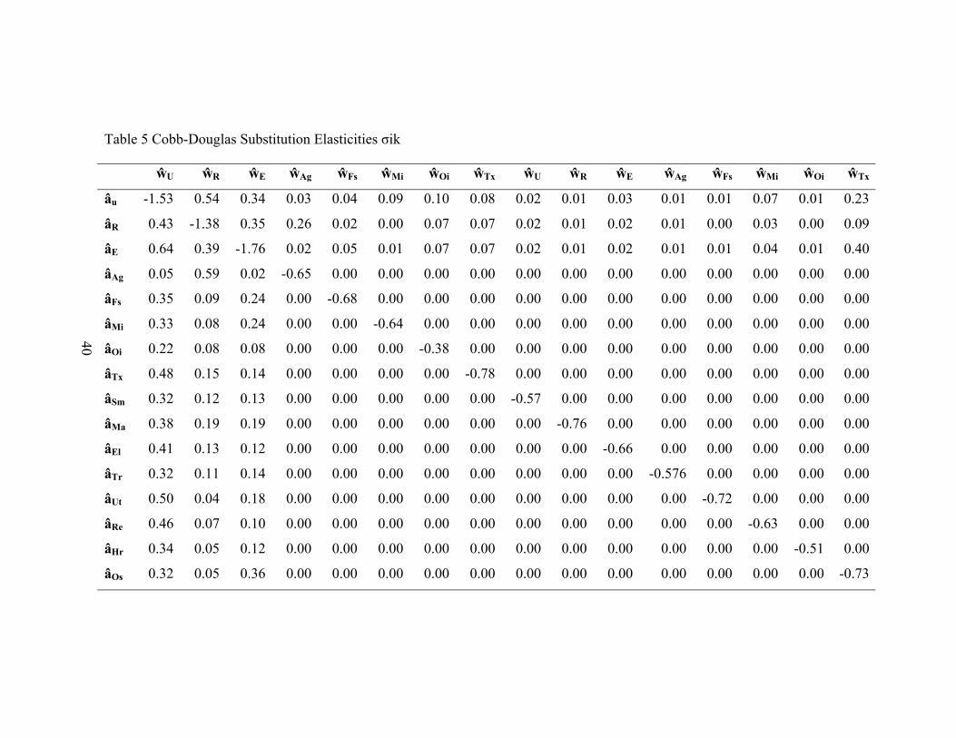
Table 5 Cobb-Douglas Substitution Elasticities σik
40
ŵU ŵR ŵE ŵAg ŵFs ŵMi ŵOi ŵTx ŵU ŵR ŵE ŵAg ŵFs ŵMi ŵOi ŵTx
âu -1.53 0.54 0.34 0.03 0.04 0.09 0.10 0.08 0.02 0.01 0.03 0.01 0.01 0.07 0.01 0.23
âR 0.43
-1.38 0.35 0.26 0.02 0.00 0.07 0.07 0.02 0.01 0.02 0.01 0.00 0.03 0.00 0.09
âE 0.64 0.39 -1.76 0.02 0.05 0.01 0.07 0.07 0.02 0.01 0.02 0.01 0.01 0.04 0.01 0.40
âAg 0.05 0.59 0.02 -0.65 0.00 0.00 0.00 0.00 0.00 0.00 0.00 0.00 0.00 0.00 0.00 0.00
âFs 0.35 0.09 0.24 0.00 -0.68 0.00 0.00 0.00 0.00 0.00 0.00 0.00 0.00 0.00 0.00 0.00
âMi 0.33 0.08 0.24 0.00 0.00 -0.64 0.00 0.00 0.00 0.00 0.00 0.00 0.00 0.00 0.00 0.00
âOi 0.22 0.08 0.08 0.00 0.00 0.00 -0.38 0.00 0.00 0.00 0.00 0.00 0.00 0.00 0.00 0.00
âTx 0.48 0.15 0.14 0.00 0.00 0.00 0.00 -0.78 0.00 0.00 0.00 0.00 0.00 0.00 0.00 0.00
âSm 0.32 0.12 0.13 0.00 0.00 0.00 0.00 0.00 -0.57 0.00 0.00 0.00 0.00 0.00 0.00 0.00
âMa 0.38 0.19 0.19 0.00 0.00 0.00 0.00 0.00 0.00 -0.76 0.00 0.00 0.00 0.00 0.00 0.00
âEl 0.41 0.13 0.12 0.00 0.00 0.00 0.00 0.00 0.00 0.00 -0.66 0.00 0.00 0.00 0.00 0.00
âTr 0.32 0.11 0.14 0.00 0.00 0.00 0.00 0.00 0.00 0.00 0.00 -0.576 0.00 0.00 0.00 0.00
âUt 0.50 0.04 0.18 0.00 0.00 0.00 0.00 0.00 0.00 0.00 0.00 0.00 -0.72 0.00 0.00 0.00
âRe 0.46 0.07 0.10 0.00 0.00 0.00 0.00 0.00 0.00 0.00 0.00 0.00 0.00 -0.63 0.00 0.00
âHr 0.34 0.05 0.12 0.00 0.00 0.00 0.00 0.00 0.00 0.00 0.00 0.00 0.00 0.00 -0.51 0.00
âOs 0.32 0.05 0.36 0.00 0.00 0.00 0.00 0.00 0.00 0.00 0.00 0.00 0.00 0.00 0.00 -0.73
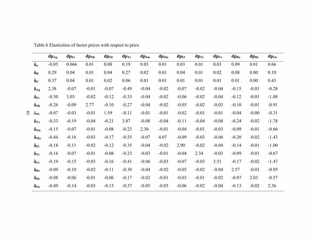
Table 6 Elasticities of factor prices with respect to price
41
dpAg dpFs dpMi dpOI dpTx dpSm dpMa dpEl dpTr dpUt dpRe dpHr dpOs
âu -0.05 0.066 0.01 0.08 0.19 0.03 0.01 0.03 0.01 0.03 0.09 0.01 0.66
âR 0.29
0.04 0.01 0.04 0.27 0.02 0.01 0.04 0.01 0.02 0.08 0.00 0.10
âE 0.37 0.04 0.01 0.02 0.06 0.01 0.01 0.01 0.01 0.01 0.01 0.00 0.43
âAg 2.38 -0.07 -0.01 -0.07 -0.49 -0.04 -0.02 -0.07 -0.02 -0.04 -0.15 -0.01 -0.28
âFs -0.30 3.03 -0.02 -0.12 -0.33 -0.04 -0.02 -0.06 -0.02 -0.04 -0.12 -0.01 -1.08
âMi -0.26 -0.09 2.77 -0.10 -0.27 -0.04 -0.02 -0.05 -0.02 -0.03 -0.10 -0.01 -0.91
âOi -0.07 -0.03 -0.01 1.59 -0.11 -0.01 -0.01 -0.02 -0.01 -0.01 -0.04 -0.00 -0.31
âTx -0.33 -0.19 -0.04 -0.21 3.87 -0.08 -0.04 -0.11 -0.04 -0.08 -0.24 -0.02 -1.78
âSm -0.15 -0.07 -0.01 -0.08 -0.23 2.30 -0.01 -0.04 -0.01 -0.03 -0.09 -0.01 -0.66
âMa -0.44 -0.16 -0.03 -0.17 -0.55 -0.07 4.07 -0.09 -0.03 -0.06 -0.20 -0.02 -1.43
âEl -0.18 -0.11 -0.02 -0.12 -0.35 -0.04 -0.02 2.90 -0.02 -0.04 -0.14 -0.01 -1.00
âTr -0.16 -0.07 -0.01 -0.08 -0.23 -0.03 -0.01 -0.04 2.34 -0.03 -0.09 -0.01 -0.67
âUt -0.19 -0.15 -0.03 -0.16 -0.41 -0.06 -0.03 -0.07 -0.03 3.51 -0.17 -0.02 -1.47
âRe -0.09 -0.10 -0.02 -0.11 -0.30 -0.04 -0.02 -0.05 -0.02 -0.04 2.57 -0.01 -0.95
âHr -0.08 -0.06 -0.01 -0.06 -0.17 -0.02 -0.01 -0.03 -0.01 -0.02 -0.07 2.03 -0.57
âOs -0.49 -0.14 -0.03 -0.13 -0.37 -0.05 -0.03 -0.06 -0.02 -0.04 -0.13 -0.02 2.36
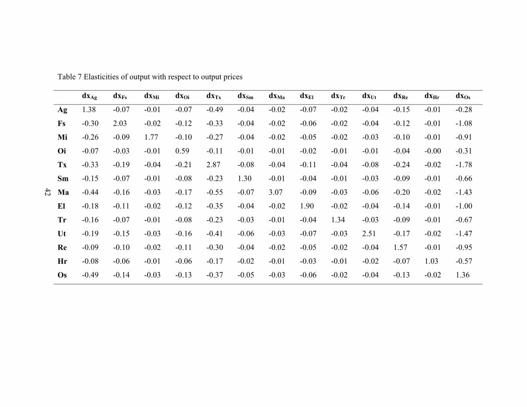
Table 7 Elasticities of output with respect to output prices
42
dxAg dxFs dxMi dxOi dxTx dxSm dxMa dxEl dxTr dxUt dxRe dxHr dxOs
Ag 1.38 -0.07 -0.01 -0.07 -0.49 -0.04 -0.02 -0.07 -0.02 -0.04 -0.15 -0.01 -0.28
Fs -0.30
2.03 -0.02 -0.12 -0.33 -0.04 -0.02 -0.06 -0.02 -0.04 -0.12 -0.01 -1.08
Mi -0.26 -0.09 1.77 -0.10 -0.27 -0.04 -0.02 -0.05 -0.02 -0.03 -0.10 -0.01 -0.91
Oi -0.07 -0.03 -0.01 0.59 -0.11 -0.01 -0.01 -0.02 -0.01 -0.01 -0.04 -0.00 -0.31
Tx -0.33 -0.19 -0.04 -0.21 2.87 -0.08 -0.04 -0.11 -0.04 -0.08 -0.24 -0.02 -1.78
Sm -0.15 -0.07 -0.01 -0.08 -0.23 1.30 -0.01 -0.04 -0.01 -0.03 -0.09 -0.01 -0.66
Ma -0.44 -0.16 -0.03 -0.17 -0.55 -0.07 3.07 -0.09 -0.03 -0.06 -0.20 -0.02 -1.43
El -0.18 -0.11 -0.02 -0.12 -0.35 -0.04 -0.02 1.90 -0.02 -0.04 -0.14 -0.01 -1.00
Tr -0.16 -0.07 -0.01 -0.08 -0.23 -0.03 -0.01 -0.04 1.34 -0.03 -0.09 -0.01 -0.67
Ut -0.19 -0.15 -0.03 -0.16 -0.41 -0.06 -0.03 -0.07 -0.03 2.51 -0.17 -0.02 -1.47
Re -0.09 -0.10 -0.02 -0.11 -0.30 -0.04 -0.02 -0.05 -0.02 -0.04 1.57 -0.01 -0.95
Hr -0.08 -0.06 -0.01 -0.06 -0.17 -0.02 -0.01 -0.03 -0.01 -0.02 -0.07 1.03 -0.57
Os -0.49 -0.14 -0.03 -0.13 -0.37 -0.05 -0.03 -0.06 -0.02 -0.04 -0.13 -0.02 1.36
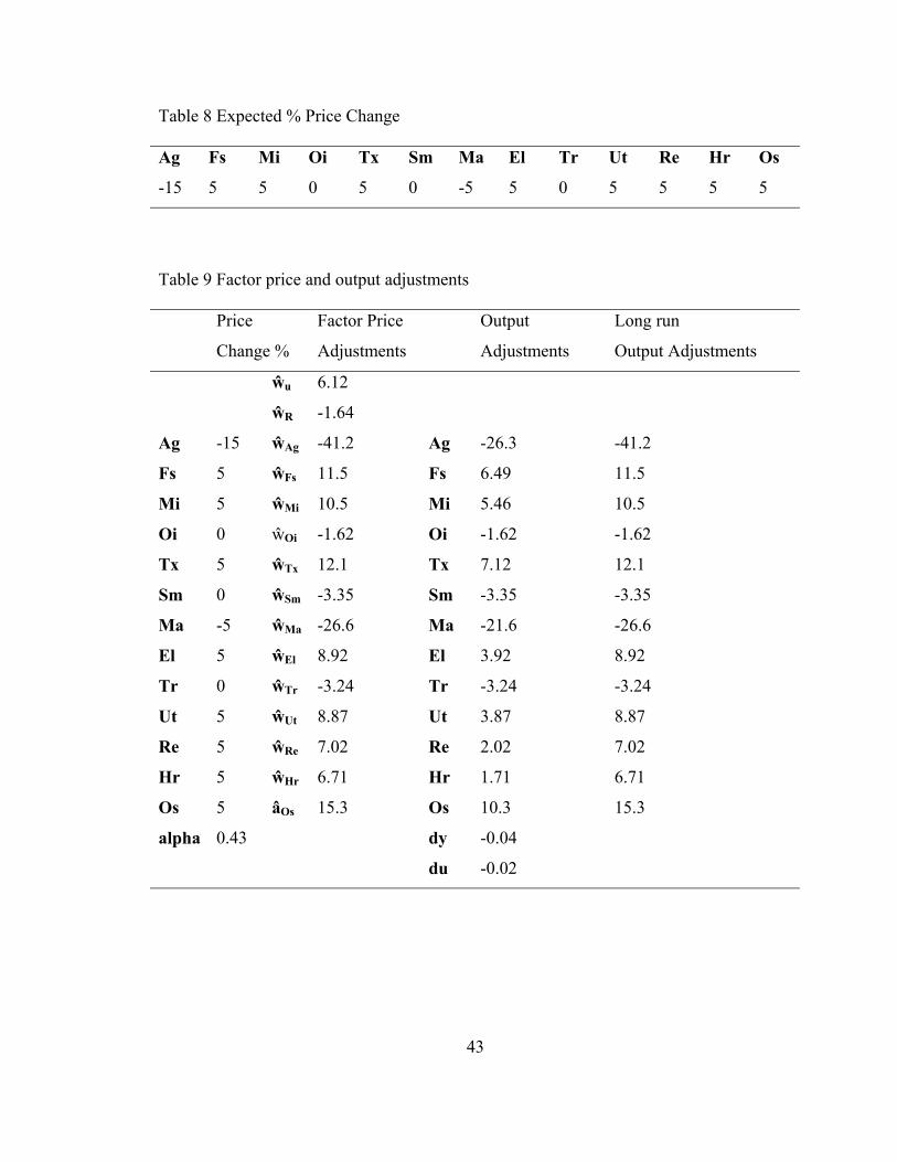
43
Table 8 Expected % Price Change
Ag Fs Mi Oi Tx Sm Ma El Tr Ut Re Hr Os
-15 5 5 0 5 0 -5 5 0 5 5 5 5
Table 9 Factor price and output adjustments
Price
Change %
Factor Price
Adjustments
Output
Adjustments
Long run
Output Adjustments
ŵu 6.12
ŵR -1.64
Ag -15 ŵAg -41.2 Ag -26.3 -41.2
Fs 5 ŵFs 11.5 Fs 6.49 11.5
Mi 5 ŵMi 10.5 Mi 5.46 10.5
Oi 0 ŵOi -1.62 Oi -1.62 -1.62
Tx 5 ŵTx 12.1 Tx 7.12 12.1
Sm 0 ŵSm -3.35 Sm -3.35 -3.35
Ma -5 ŵMa -26.6 Ma -21.6 -26.6
El 5 ŵEl 8.92 El 3.92 8.92
Tr 0 ŵTr -3.24 Tr -3.24 -3.24
Ut 5 ŵUt 8.87 Ut 3.87 8.87
Re 5 ŵRe 7.02 Re 2.02 7.02
Hr 5 ŵHr 6.71 Hr 1.71 6.71
Os 5 âOs 15.3 Os 10.3 15.3
alpha 0.43 dy -0.04
du -0.02
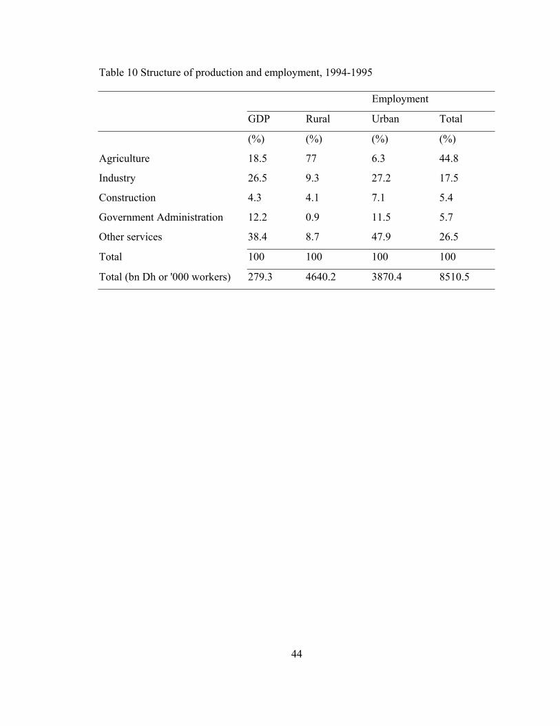
44
Table 10 Structure of production and employment, 1994-1995
Employment
GDP Rural Urban Total
(%) (%) (%) (%)
Agriculture 18.5 77 6.3 44.8
Industry 26.5 9.3 27.2 17.5
Construction 4.3 4.1 7.1 5.4
Government Administration 12.2 0.9 11.5 5.7
Other services 38.4 8.7 47.9 26.5
Total 100 100 100 100
Total (bn Dh or '000 workers) 279.3 4640.2 3870.4 8510.5
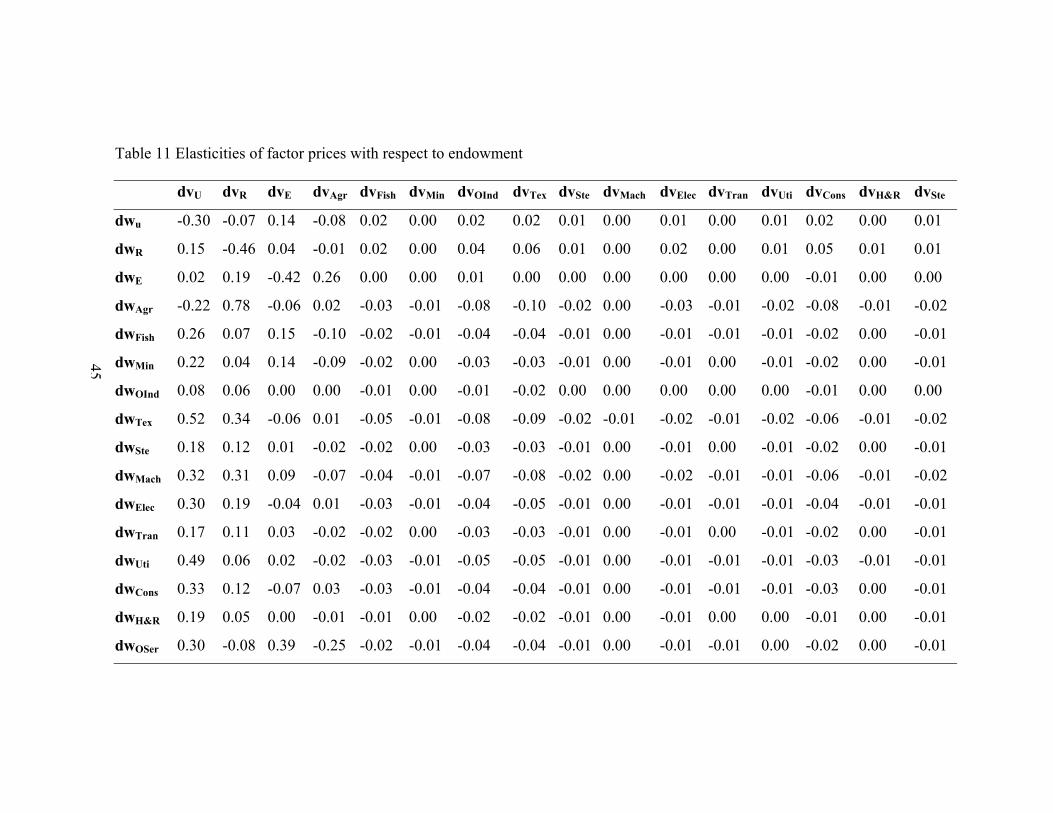
Table 11 Elasticities of factor prices with respect to endowment
dvU dvR dvE dvAgr dvFish dvMin dvOInd dvTex dvSte dvMach dvElec dvTran dvUti dvCons dvH&R dvSte
dwu -0.30 -0.07 0.14 -0.08 0.02 0.00 0.02 0.02 0.01 0.00 0.01 0.00 0.01 0.02 0.00 0.01
dwR 0.15
-0.46 0.04 -0.01 0.02 0.00 0.04 0.06 0.01 0.00 0.02 0.00 0.01 0.05 0.01 0.01
dwE 0.02 0.19 -0.42 0.26 0.00 0.00 0.01 0.00 0.00 0.00 0.00 0.00 0.00 -0.01 0.00 0.00
dwAgr -0.22 0.78 -0.06 0.02 -0.03 -0.01 -0.08 -0.10 -0.02 0.00 -0.03 -0.01 -0.02 -0.08 -0.01 -0.02
dwFish 0.26 0.07 0.15 -0.10 -0.02 -0.01 -0.04 -0.04 -0.01 0.00 -0.01 -0.01 -0.01 -0.02 0.00 -0.01
dwMin 0.22 0.04 0.14 -0.09 -0.02 0.00 -0.03 -0.03 -0.01 0.00 -0.01 0.00 -0.01 -0.02 0.00 -0.01
dwOInd 0.08 0.06 0.00 0.00 -0.01 0.00 -0.01 -0.02 0.00 0.00 0.00 0.00 0.00 -0.01 0.00 0.00
dwTex 0.52 0.34 -0.06 0.01 -0.05 -0.01 -0.08 -0.09 -0.02 -0.01 -0.02 -0.01 -0.02 -0.06 -0.01 -0.02
dwSte 0.18 0.12 0.01 -0.02 -0.02 0.00 -0.03 -0.03 -0.01 0.00 -0.01 0.00 -0.01 -0.02 0.00 -0.01
dwMach 0.32 0.31 0.09 -0.07 -0.04 -0.01 -0.07 -0.08 -0.02 0.00 -0.02 -0.01 -0.01 -0.06 -0.01 -0.02
dwElec 0.30 0.19 -0.04 0.01 -0.03 -0.01 -0.04 -0.05 -0.01 0.00 -0.01 -0.01 -0.01 -0.04 -0.01 -0.01
dwTran 0.17 0.11 0.03 -0.02 -0.02 0.00 -0.03 -0.03 -0.01 0.00 -0.01 0.00 -0.01 -0.02 0.00 -0.01
dwUti 0.49 0.06 0.02 -0.02 -0.03 -0.01 -0.05 -0.05 -0.01 0.00 -0.01 -0.01 -0.01 -0.03 -0.01 -0.01
dwCons 0.33 0.12 -0.07 0.03 -0.03 -0.01 -0.04 -0.04 -0.01 0.00 -0.01 -0.01 -0.01 -0.03 0.00 -0.01
dwH&R 0.19 0.05 0.00 -0.01 -0.01 0.00 -0.02 -0.02 -0.01 0.00 -0.01 0.00 0.00 -0.01 0.00 -0.01
dwOSer 0.30 -0.08 0.39 -0.25 -0.02 -0.01 -0.04 -0.04 -0.01 0.00 -0.01 -0.01 0.00 -0.02 0.00 -0.01
45
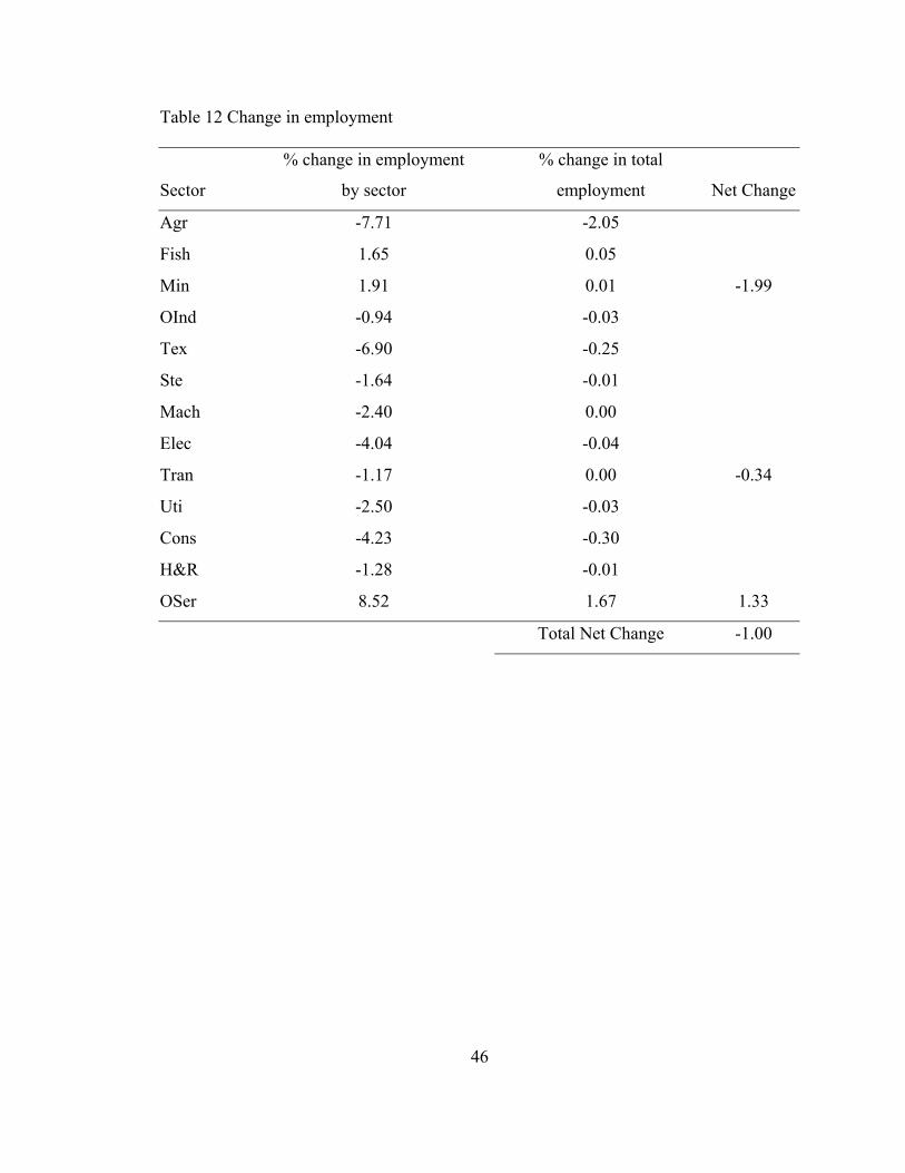
46
Table 12 Change in employment
Sector
% change in employment
by sector
% change in total
employment Net Change
Agr -7.71 -2.05
Fish 1.65 0.05
Min 1.91 0.01 -1.99
OInd -0.94 -0.03
Tex -6.90 -0.25
Ste -1.64 -0.01
Mach -2.40 0.00
Elec -4.04 -0.04
Tran -1.17 0.00 -0.34
Uti -2.50 -0.03
Cons -4.23 -0.30
H&R -1.28 -0.01
OSer 8.52 1.67 1.33
Total Net Change -1.00
47
CHAPTER 2. AN EMPIRICAL STUDY OF RESTRICTED CAPITAL MOBILITY
AND EXCHANGE RATES
1. Introduction
The literature on floating exchange rates has looked at relative money supplies
when analyzing exchange rates and relative price levels. The literature includes Branson
(1986), Bilson (1978), Driskil (1976), Henderson (1980), Balassa (1964), and Frankel
(1979). While this literature has provided a rich array of predictions and long-run
relationships between money, exchange rates, and price levels, it has provided very little
insight into exchange rate behavior in response to economic growth and different levels
of capital mobility.
The purpose of the present paper is to evaluate the impact of different levels of
capital mobility on the exchange rate applying an open economy macroeconomic
framework and using two structural models, the monetary model and a stock-flow model
developed by generalizing the Dornbusch model to allow imperfect capital mobility. The
case examined is South Korea relative to Ireland from 1974 to 1998 covering the post
Bretton Woods system up to Ireland’s adoption of the euro.
The demand for money function and the assumption of uncovered interest parity
in the monetary model and the Dornbusch model are very similar but the two models
yield different results. The model proposed by Dornbusch (1976) has a money demand
48
function similar to that presented in the basic monetary model of Keynes where the
demand for money is a function of income, price, and interest rate:
M = kPYα e-βi (1)
where M represents the domestic money stock, k is a parameter that takes account of
factors (such as real income) that affect the demand of real money, P is the price level, Y
is income, and i is the domestic interest rate.
The Dornbusch model also assumes perfect capital mobility, implied by
uncovered interest parity:
i – i*= E(Ŝ) (2)
where the interest rate differential i – i* is equal to the expected change in the exchange
rate.
Korea and Ireland are two small open economies that have experienced
continuous economic growth over the last three decades. Ireland has had relatively less
restrictions on capital mobility than Korea and has seen its currency continuously
appreciate relative to South Korea’s won between 1974 and 1998. Figure 1 shows the
appreciation of Irish punt relative to the South Korean won from 1974 to 1998.
Korea and Ireland are not major trading partners, and both countries are small open
economies and price takers in the foreign exchange market. The won and the punt are
traded publicly in the international exchange rate market. The US is a trading partner for
both. The “triangular” exchange rate between won, the US dollar, and punt equalizes
rates. Any disparity in the indirect exchange rate between the won to the punt via the
dollar or any other currency would be eliminated by arbitrage. Two small open

49
economies do not need to be trading partners in order to evaluate the relative change in
the value of their respective currencies.
The monetary model assumes price flexibility and competition in trade to make
exchange rate analysis relatively uncomplicated. Hacche and Townend (1981) argue that
it is unique in the way in which its special assumptions about price flexibility and
competition in trade simplify analysis by allowing the exchange rate to be regarded as the
price that clears the money market in a small open economy. Four models of exchange
rate determination are discussed below.
2. Survey of Exchange Rate Models
2.1. Mundell-Fleming Model
The Mundell-Fleming model is a small open economy IS-LM framework that can
be used to analyze the influence of monetary policy on the exchange rate following
Fleming (1962) and Mundell (1963). Dornbush (1980) calls the Mundell-Fleming model
“the backbone of macroeconomic models of the exchange rate.” The model assumes
domestic price levels are constant and the output level is determined at given levels of
foreign trade and capital flows. The model also assumes foreign price levels and foreign
real incomes are exogenous with net exports a decreasing function of domestic real
income and the exchange rate. Imports are assumed price elastic. The foreign interest
rate is exogenous.
Net inflow of capital is assumed to be an increasing function of the domestic
interest rate and the expected rate of depreciation. With uncovered interest rate parity, an
increase in the domestic interest rate or depreciation of the home currency will cause a
ceteris paribus inflow of foreign capital. When the domestic interest rate increases,
50
foreign investors increase their holdings of domestic bonds and an inflow of capital
results. Similarly, depreciation causes an inflow of foreign capital as domestic exports
become relatively cheaper and foreign importers increase their demand for domestic
exports.
The Mundell-Fleming model in Figure 2 assumes perfect capital mobility and a
floating exchange rate, and analyzes the influence of an increase in the money supply on
the exchange rate starting from a position of equilibrium where the goods and the money
markets are in equilibrium and the external payments balanced. The model considers an
exogenous increase in the money supply which puts downward pressure on the interest
rate in the short run. The decreasing interest rates would in turn stimulate interest
sensitive expenditures and income increases. The excess supply of money will be
eliminated through a decrease in the interest rate and an increase in income but a balance
of payment deficit would develop. To eliminate the deficit, the domestic currency
depreciates. In sum, the Mundell-Fleming model predicts that domestic monetary
expansion leads to depreciation. The external balance is maintained primarily through
the current account and equilibrium in money and goods markets is re-established by a
combination of lower interest rates and higher output.
The Mundell-Fleming model allows different levels of capital mobility and
economic growth. When applying the IS-LM-BP framework, an increase in domestic
income could cause either an appreciation or a depreciation of the domestic currency
depending on capital mobility.
Given international trade in goods and services as well as assets, its balance of
payment B is represented by:
51
B = T(q, Y) + K(i-i*) (3)
The trade balance depends on the relative price of foreign goods in terms of domestic
goods q and on domestic income Y. The capital account K depends on the interest rate
differential. The capital account is positive when there is net inflow of capital and
negative when there is a net outflow of capital. The BP equilibrium is achieved when
there are no surpluses and no deficits,
B = T(q, Y) + K(i-i*) = 0 (3’)
Capital mobility and the BP slope are determined by the interest elasticity of the capital
account. In Figure 3, an economy that is facing no capital mobility without international
trade in financial assets has a zero capital account so that the balance of payments is
made up solely of the current account which is not a function of the interest rate. The
balance of payments locus is then represented by the vertical line T = 0 and is perfectly
interest inelastic.
For an economy with imperfect capital mobility, with the balance of payments
(BOP) and balance of trade (BOT) initially balanced. At any given interest rate, an
increase in income causes imports to increase and the trade balance to deteriorate, and
moves the economy into payments and trade account deficits. Assuming fixed exchange
rates to correct for the trade deficit, the domestic interest rate increases to make domestic
bonds more attractive relative to foreign bonds and entice capital inflow. The inflow of
capital generates a capital account surplus and improves the balance of payments by
offsetting the trade balance deficit.
For any given level of capital mobility there can be an increase of interest rate
large enough to induce capital inflow necessary to eliminate the balance of payments
52
deficit. As domestic income increases, balanced of payments can be maintained through
the capital account by an appropriate increase in the domestic interest rate, and the BOP
equilibrium locus for an economy with imperfect capital mobility is represented by the
upward sloping schedule labeled B = 0.
The final alternative is an economy with perfect capital mobility in which balance
of payments equilibrium can occur only if the economy is on the perfectly horizontal BB
locus. An increase in domestic income will result in an increase in imports and a
worsening of the trade balance. To restore a payments balance in the case of an economy
with imperfect capital mobility, the interest rate would have to increase to induce inflows
of capital. In the case of an economy with perfect capital mobility, the interest rate does
not have to increase to induce inflows of capital because any amount necessary to balance
the payments is available in the world capital market at the world rate i*. The BP locus
for an economy with perfect capital mobility is perfectly horizontal or perfectly interest
elastic.
Starting with a model similar to the Mundell-Fleming model in Figure 1 but
severely restricting the mobility of capital, an increase in income would cause the
currency to depreciate in Figure 4. The IS curve is a schedule of interest rate and
corresponding domestic income that keep the domestic goods market in equilibrium.
Two key assumptions are made when the IS curve is derived with government spending
and the relative price of foreign goods in terms of domestic goods constant. When the
economy is below full employment, an increase in income can come about either as a
result of government policy intervention through an increase in government spending or a
53
decrease in taxes, or as long-run adjustment to expansionary monetary policy. Such an
exogenous increase in spending is represented by a rightward shift in the IS curve.
One of the main ideas of Keynesian economics is that in the short run the equilibrium
level of output can be trapped below full employment resulting in chronic unemployment
and recession. Government policy intervention is then believed to be vital in moving the
economy out of recession, with increased government spending having a leading role in
that recovery. But government policy intervention or any real disturbance is believed to
be ineffective when exchange rates are flexible. A real disturbance is any exogenous
disturbance that does not change the money demand or money supply or originate in the
money market as a nominal disturbance.
One of the implications of the Mundell-Fleming model is that fiscal policy under
a flexible exchange rate is ineffective. It is also argued (Barro, 1990) that real
disturbances would not have any effect on output but would only affect the exchange
rate. McKibbin and Sachs (1991) use a sophisticated dynamic Mundell-Fleming model
to show that commercial policy in the form of protection against imports (a real
disturbance) would not have any lasting effect on output and would only result in
exchange rate appreciation. The assumptions of full employment and perfect capital
mobility in the Mundell-Fleming model affect the effectiveness of real disturbances on
output. Relaxing those assumptions would alter the effect of real disturbances on output
and the exchange rate.
In Figures 4 and 5 the assumptions of perfect capital mobility and full
employment have been relaxed. Figure 4 represents an economy where capital mobility
is less restricted relative to the economy in Figure 5. The relatively more mobile capital
54
in Figure 4 is shown by the flatter BP and steeper LM curves. In Figure 5 capital is less
mobile and is shown by a steeper BP curve and a flatter LM curve. An increase in
income would cause the currency of the economy with more mobile capital to appreciate
and the currency of the economy with less mobile capital to depreciate.
The Mundell-Fleming model has shortcomings in light of more recent theoretical
developments. There are no explicit dynamics and lags in the response of output and
trade, there is no price response to either monetary shocks or currency depreciation, and
the interest rate effect on the capital flows seems permanent and non-eroding. Portfolio
balance models also assume BOP equilibrium but offer a more comprehensive analysis
by taking into account asset preferences and the requirements for portfolio balance.
2.2. Portfolio Balance Models
Portfolio balance models focus on requirements for stock equilibrium in the
markets for domestic money, domestic assets, and foreign assets. While the Mundell-
Fleming model focuses on requirements for flow equilibrium in the goods market and the
balance of payments, Branson and Halttunen (1979) use a portfolio balance model where
domestic residents are the exclusive holders of domestic money and bonds. Domestic
residents also hold foreign bonds which represent the only tradable asset, and domestic
assets and foreign assets are assumed to be gross substitutes. A fall in domestic holding
of foreign bonds represents an increase in liabilities to foreign countries. The ratio of
wealth domestic residents wants to hold in each asset is dependent on relative expected
common currency yields.
The exchange rate has three separate effects. First, exchange rates change the
value of foreign assets in terms of domestic currency. Total wealth in nominal domestic
55
currency will rise with depreciation and fall with appreciation. Second, exchange rate
expectations are an integral part of the relative yields of domestic and foreign assets.
Third, exchange rates affect the current account and the net acquisition of foreign assets.
Portfolio balance models view the exchange rate in the short run as determined by
the balance of asset markets, the accumulation of foreign assets, and lagged response on
the current account. In the long run the current account is balanced.
Consider the effect of an increase in the money supply through the purchase of
domestic bonds by the domestic central bank assuming that the original equilibrium is a
full equilibrium with asset supplies fixed and a balance of payment equal to zero. The
increased money supply will cause an excess demand for domestic bonds and excess
supply of money at the original interest rate and exchange rate. Return to equilibrium in
the domestic assets market will require domestic interest rate to drop. The excess
demand for domestic bonds bids the prices of domestic bonds up or domestic interest rate
down. The drop in domestic interest rate makes domestic bonds a less attractive asset.
The lower interest rate in turn will cause an increase in the demand for foreign bonds that
can be eliminated by depreciation. The new asset equilibrium represents short run
equilibrium and is achieved by a lower interest rate and depreciation.
The current account at the initial equilibrium is balanced, with positive investment
income offset by a trade deficit since the domestic country is a net creditor in the foreign
bond market. The adjustment to the new equilibrium will not have any effect on the
current account at first since the lower interest rate and depreciated currency have
restored portfolio balance with net foreign bonds unchanged. The increase in foreign
bond holding produced by lower domestic interest rate is offset by the sale of foreign
56
bonds produced by the effect of depreciation on the composition of wealth. With goods
prices unaffected, the new equilibrium will cause deterioration in the terms of trade that
will affect net exports and net foreign assets.
If the usual conditions on price elasticities of trade hold, depreciation will cause a
current account surplus and an increase in net foreign assets, upsetting the portfolio
balance. The new equilibrium is transitory. These new disturbances cause an excess
supply of foreign bonds and a parallel excess demand for domestic assets. To restore
portfolio balance the domestic currency appreciates reducing net exports and
consequently slowing growth. The increase in net foreign assets will increase net
investment income push the current account into further surplus. For stability, trade
elasticities are assumed to be large enough so the reduction in net exports outweighs the
increase in net investment income. The current account surplus produced by the initial
depreciation is eliminated and equilibrium reestablished.
The exchange rate in its adjustment to the long run equilibrium is at first higher
than in the temporary asset equilibrium but decreases as the current account re-balances.
This overshooting of the exchange rate is explained by the assumption that exchange
rates and interest rates respond quickly to monetary shocks to maintain portfolio balance,
while trade takes a longer time to adjust. In the long run the current account is balanced
but with lower net exports and higher net investment income since net foreign assets have
increased.
The change in the exchange rate will depend on whether the change of the money
supply had any effect on real income. If there has been no growth in real income, the
exchange rate will be higher than at the outset because the increase in the money supply
57
would cause a proportional increase in the price level and less than proportional
depreciation. If monetary expansion results in an increase in real income, the direction of
change in the exchange rate will be ambiguous.
2.3. Monetary Model
The monetary model of exchange rates is based on money market equilibrium and
can be considered a version of the portfolio balance model. The exchange rate is
determined by the purchasing power parity condition (PPP).
The basic monetary model assumes perfect capital mobility, PPP, and price levels
implied by PPP such that the demand and the supply of money match for given levels of
real outputs, interest rates, and exchange rate. Figure 2 illustrates the basic monetary
model using the IS-LM-BP framework. At a given level of real output (full employment)
the IS curve is vertical and a horizontal balance of payment (BP) shows perfect capital
mobility. The equilibrium exchange rate is such that the LM curve intersects the IS curve
at the interest rate given by the perfect capital mobility.
The basic monetary model can be set out as three structural equations, a demand
for money equation, where the demand for money is a function of the price level P, real
income Y, and interest rate i,
m = lnk + p + αy - βi (1’)
where m represents the logarithm of domestic money stock, k is a parameter that takes
account of factors (such as real income) that affect the demand of real money, and p and
y are the logarithms of the price level and income respectively. The foreign demand for
money is based on similar assumptions and is identical to the domestic demand for
money with * superscript to denote foreign variables and parameters.
58
The exchange rate S represents the foreign currency price of domestic currency
and is given by the PPP as the ratio between foreign and domestic price levels.
S = κP/P* (4)
where κ is a constant, not necessarily 1. Substituting and logarithmic transformation of
(4) gives the following equation
s = K – m + m* + αy – α*y*– βi + β*i* (5)
where K = lnk - lnk* + lnκ. Equation (5) may be estimated as the reduced form of the
system, with the right hand variables assumed exogenous.
According to the monetary approach, changes in the variables will affect money
market equilibrium which in turn affects the exchange rate. The model predicts that an
increase in the domestic money supply will cause a proportional depreciation of the
domestic currency. The assumptions of PPP and unit price elasticity in the demand for
money force elasticity of the exchange rate with respect to domestic money supply to
equal -1 and with respect to foreign money supply to equal 1.
In the adjustment to monetary expansion, an increase in the money supply will
cause an increase in demand for goods and assets. Domestic residents have two possible
mechanisms to dispose of the excess supply of money. The first mechanism operates
through a trade deficit and reduces the money balances as the domestic residents increase
their purchase of foreign goods. The trade balance deficit causes a reduction of total
domestic assets and represents a portfolio-size adjustment. The second mechanism
operates through a capital account deficit as the excess supply of money is used to
purchase foreign assets. The exchange of money to acquire foreign assets affects the
composition of the portfolio but not the size of the total portfolio and represents a
59
portfolio-composition adjustment. Since all variables are assumed exogenously
determined, they do not respond to a monetary shock. Real output is at its full
employment level, domestic prices are tied by international competition and cannot
respond directly, and the domestic interest rate is tied to the foreign interest rate and
exchange rate expectations by uncovered interest rate parity in (2).
The resulting disequilibrium causes excess demand for foreign goods and assets
leading to depreciation. Domestic prices rise to restore equilibrium, consistent with PPP.
The real money supply is unchanged since the price elasticity of money demand is
unitary. The rise in the price level and depreciation are proportional to the increase in the
money supply. The basic monetary model regards the exchange rate as the effective
“price” that clears the domestic money market through the domestic price level. The
domestic price level is flexible to maintain PPP.
Most studies following the monetary approach assume that higher domestic
income relative to foreign income leads to an increase in domestic transactions. This
higher rate of domestic transactions results in a higher money demand relative to foreign
money demand causing appreciation.
The monetary model predicts that a rise in the domestic interest rate will lower the
exchange rate by causing an excess supply of money. The money market equilibrium is
determined by the price level and exchange rate. The domestic interest rate is exogenous
and must satisfy the uncovered interest rate parity in (2). For a given foreign interest rate
i* the domestic interest rate is determined by exchange rate expectations. A rise in the
interest rate i is the result of change in exchange rate expectations. The change in interest
rate differential represents the expected depreciation of the domestic currency, consistent
60
with uncovered interest parity and not corresponding to an increase in the expected
relative yield of domestic assets.
The expected change in the exchange rate E(ŝ) must be assumed exogenous to the
current exchange rate and its determinants when estimating (5) as the reduced form for
the exchange rate. This assumption is inconsistent with the rational expectations
hypothesis (RE). The exogeneity assumption can be maintained if exchange rate changes
are assumed to depend on market perceptions of inflation and conditions in the money
market, perhaps unresponsive in the short run to changes in the determinants of the
current exchange rate. This last condition is inconsistent with the basic monetary model.
When expectations are assumed to be rational, the domestic interest rate and the interest
rate differential become endogenous as in Mussa (1976). To endogenize the domestic
interest rate and the interest rate differential (2) can be rewritten as
it – it*= st – Etst+1 (6)
where st represents the logarithm of the exchange rate at time t and Etst+1 represents the
expectation of percentage change in the exchange rate at time t+1 given information
available at time t. Substituting (6) into (5) gives
st = (1/1–β)Zt + (β / 1+ β) Et st+1 (7)
where Z = K – m + m* + αy – α*y*– (β* + β)i*.
The rational expectation of the exchange rate in any future time period t+j can be
expressed as a function of the expected value of the composite exogenous variable Z plus
the expected exchange rate in the following period t+j+1.
Deriving the reduced form of the exchange rate,
st = (1/(1–β)) Σj∞
=0 (β/(1+ β))j EtZt+j (8)
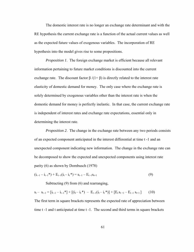
61
The domestic interest rate is no longer an exchange rate determinant and with the
RE hypothesis the current exchange rate is a function of the actual current values as well
as the expected future values of exogenous variables. The incorporation of RE
hypothesis into the model gives rise to some propositions.
Proposition 1. The foreign exchange market is efficient because all relevant
information pertaining to future market conditions is discounted into the current
exchange rate. The discount factor β /(1+ β) is directly related to the interest rate
elasticity of domestic demand for money. The only case where the exchange rate is
solely determined by exogenous variables other than the interest rate is when the
domestic demand for money is perfectly inelastic. In that case, the current exchange rate
is independent of interest rates and exchange rate expectations, essential only in
determining the interest rate.
Proposition 2. The change in the exchange rate between any two periods consists
of an expected component anticipated in the interest differential at time t -1 and an
unexpected component indicating new information. The change in the exchange rate can
be decomposed to show the expected and unexpected components using interest rate
parity (6) as shown by Dornbusch (1978)
(it -1 – it -1*) + Et -1(it – it *) = st -1 – Et -1st+1 (9)
Subtracting (9) from (6) and rearranging,
st – st -1 = [it -1 – it -1*] + [(it – it *) – Et -1(it – it *)] + [Et st +1 – Et -1 st+1 ] (10)
The first term in square brackets represents the expected rate of appreciation between
time t -1 and t anticipated at time t -1. The second and third terms in square brackets
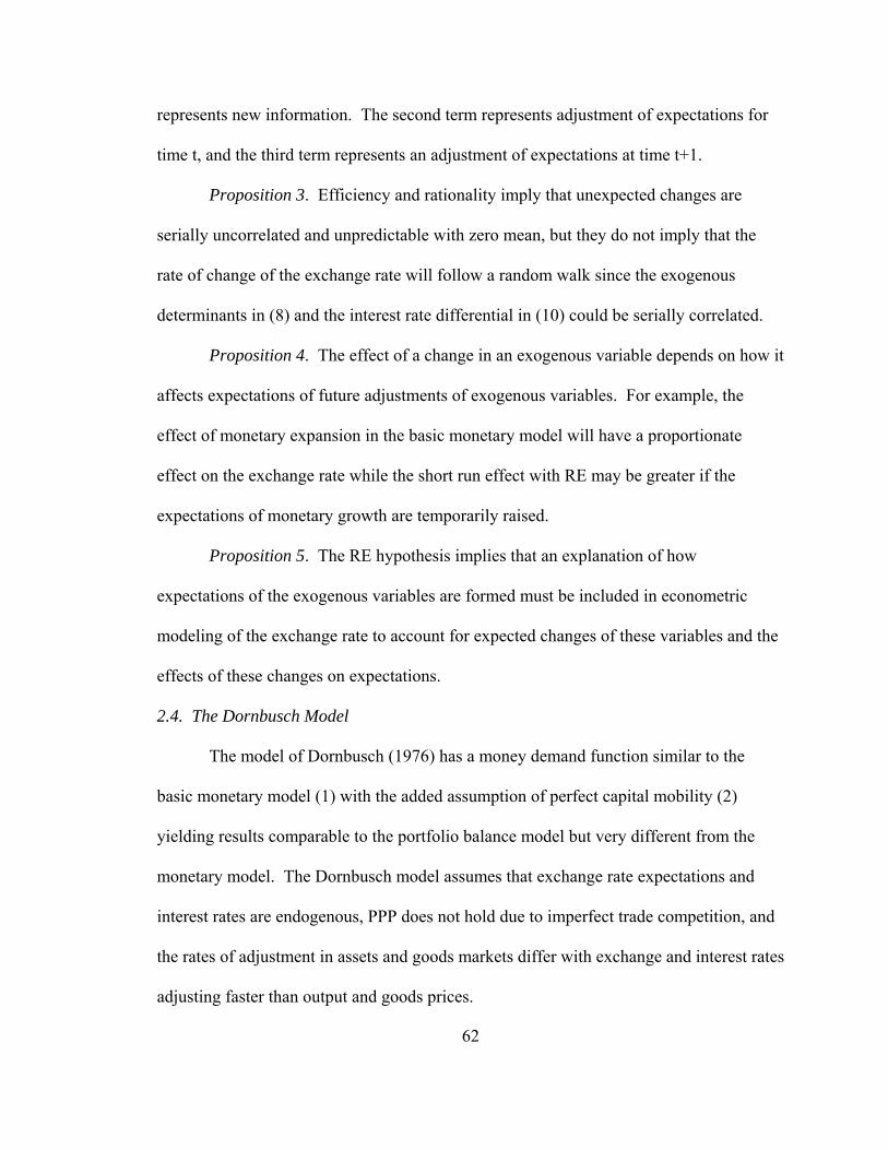
62
represents new information. The second term represents adjustment of expectations for
time t, and the third term represents an adjustment of expectations at time t+1.
Proposition 3. Efficiency and rationality imply that unexpected changes are
serially uncorrelated and unpredictable with zero mean, but they do not imply that the
rate of change of the exchange rate will follow a random walk since the exogenous
determinants in (8) and the interest rate differential in (10) could be serially correlated.
Proposition 4. The effect of a change in an exogenous variable depends on how it
affects expectations of future adjustments of exogenous variables. For example, the
effect of monetary expansion in the basic monetary model will have a proportionate
effect on the exchange rate while the short run effect with RE may be greater if the
expectations of monetary growth are temporarily raised.
Proposition 5. The RE hypothesis implies that an explanation of how
expectations of the exogenous variables are formed must be included in econometric
modeling of the exchange rate to account for expected changes of these variables and the
effects of these changes on expectations.
2.4. The Dornbusch Model
The model of Dornbusch (1976) has a money demand function similar to the
basic monetary model (1) with the added assumption of perfect capital mobility (2)
yielding results comparable to the portfolio balance model but very different from the
monetary model. The Dornbusch model assumes that exchange rate expectations and
interest rates are endogenous, PPP does not hold due to imperfect trade competition, and
the rates of adjustment in assets and goods markets differ with exchange and interest rates
adjusting faster than output and goods prices.
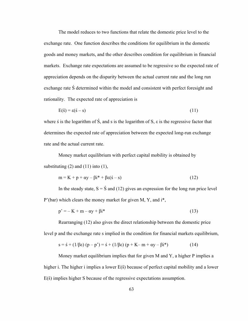
63
The model reduces to two functions that relate the domestic price level to the
exchange rate. One function describes the conditions for equilibrium in the domestic
goods and money markets, and the other describes condition for equilibrium in financial
markets. Exchange rate expectations are assumed to be regressive so the expected rate of
appreciation depends on the disparity between the actual current rate and the long run
exchange rate Ś determined within the model and consistent with perfect foresight and
rationality. The expected rate of appreciation is
E(ŝ) = ε(ś – s) (11)
where ś is the logarithm of Ś, and s is the logarithm of S, ε is the regressive factor that
determines the expected rate of appreciation between the expected long-run exchange
rate and the actual current rate.
Money market equilibrium with perfect capital mobility is obtained by
substituting (2) and (11) into (1),
m = K + p + αy – βi* + βε(ś – s) (12)
In the steady state, S = Ś and (12) gives an expression for the long run price level
P’(bar) which clears the money market for given M, Y, and i*,
p’ = – K + m – αy + βi* (13)
Rearranging (12) also gives the direct relationship between the domestic price
level p and the exchange rate s implied in the condition for financial markets equilibrium,
s = ś + (1/βε) (p – p’) = ś + (1/βε) (p + K– m + αy – βi*) (14)
Money market equilibrium implies that for given M and Y, a higher P implies a
higher i. The higher i implies a lower E(ŝ) because of perfect capital mobility and a lower
E(ŝ) implies higher S because of the regressive expectations assumption.
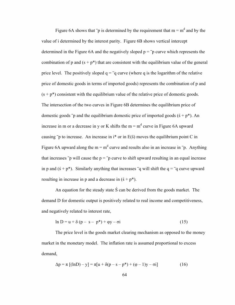
64
Figure 6A shows that ⎯p is determined by the requirement that m = md and by the
value of i determined by the interest parity. Figure 6B shows vertical intercept
determined in the Figure 6A and the negatively sloped p = ⎯p curve which represents the
combination of p and (s + p*) that are consistent with the equilibrium value of the general
price level. The positively sloped q = ⎯q curve (where q is the logarithm of the relative
price of domestic goods in terms of imported goods) represents the combination of p and
(s + p*) consistent with the equilibrium value of the relative price of domestic goods.
The intersection of the two curves in Figure 6B determines the equilibrium price of
domestic goods ⎯p and the equilibrium domestic price of imported goods (ś + p*). An
increase in m or a decrease in y or K shifts the m = md curve in Figure 6A upward
causing ⎯p to increase. An increase in i* or in E(ŝ) moves the equilibrium point C in
Figure 6A upward along the m = md curve and results also in an increase in ⎯p. Anything
that increases ⎯p will cause the p = ⎯p curve to shift upward resulting in an equal increase
in p and (ś + p*). Similarly anything that increases ⎯q will shift the q = ⎯q curve upward
resulting in increase in p and a decrease in (ś + p*).
An equation for the steady state Ś can be derived from the goods market. The
demand D for domestic output is positively related to real income and competitiveness,
and negatively related to interest rate,
ln D = u + δ (p – s – p*) + φy – σi (15)
The price level is the goods market clearing mechanism as opposed to the money
market in the monetary model. The inflation rate is assumed proportional to excess
demand,
∆p = π [(lnD) – y] = π[u + δ(p – s – p*) + (φ – 1)y – σi] (16)
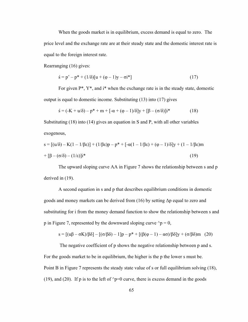
65
When the goods market is in equilibrium, excess demand is equal to zero. The
price level and the exchange rate are at their steady state and the domestic interest rate is
equal to the foreign interest rate.
Rearranging (16) gives:
ś = p’ – p* + (1/δ)[u + (φ – 1)y – σi*] (17)
For given P*, Y*, and i* when the exchange rate is in the steady state, domestic
output is equal to domestic income. Substituting (13) into (17) gives
ś = (-K + u/δ) – p* + m + [-α + (φ – 1)/δ]y + [β – (σ/δ)]i* (18)
Substituting (18) into (14) gives an equation in S and P, with all other variables
exogenous,
s = [(u/δ) – K(1 – 1/βε)] + (1/βε)p – p* + [-α(1 – 1/βε) + (φ – 1)/δ]y + (1 – 1/βε)m
+ [β – (σ/δ) – (1/ε)]i* (19)
The upward sloping curve AA in Figure 7 shows the relationship between s and p
derived in (19).
A second equation in s and p that describes equilibrium conditions in domestic
goods and money markets can be derived from (16) by setting ∆p equal to zero and
substituting for i from the money demand function to show the relationship between s and
p in Figure 7, represented by the downward sloping curve ^p = 0,
s = [(uβ – σK)/βδ] – [(σ/βδ) – 1]p – p* + [(β(φ – 1) – ασ)/βδ]y + (σ/βδ)m (20)
The negative coefficient of p shows the negative relationship between p and s.
For the goods market to be in equilibrium, the higher is the p the lower s must be.
Point B in Figure 7 represents the steady state value of s or full equilibrium solving (18),
(19), and (20). If p is to the left of ^p=0 curve, there is excess demand in the goods
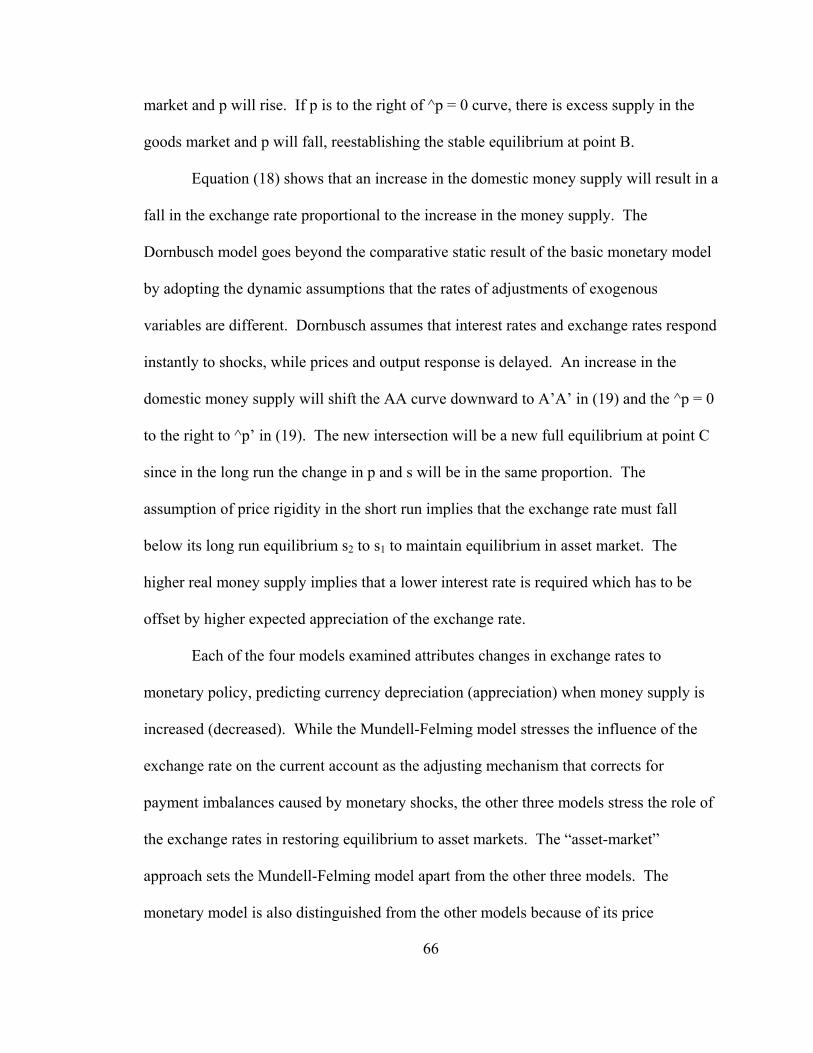
66
market and p will rise. If p is to the right of ^p = 0 curve, there is excess supply in the
goods market and p will fall, reestablishing the stable equilibrium at point B.
Equation (18) shows that an increase in the domestic money supply will result in a
fall in the exchange rate proportional to the increase in the money supply. The
Dornbusch model goes beyond the comparative static result of the basic monetary model
by adopting the dynamic assumptions that the rates of adjustments of exogenous
variables are different. Dornbusch assumes that interest rates and exchange rates respond
instantly to shocks, while prices and output response is delayed. An increase in the
domestic money supply will shift the AA curve downward to A’A’ in (19) and the ^p = 0
to the right to ^p’ in (19). The new intersection will be a new full equilibrium at point C
since in the long run the change in p and s will be in the same proportion. The
assumption of price rigidity in the short run implies that the exchange rate must fall
below its long run equilibrium s2 to s1 to maintain equilibrium in asset market. The
higher real money supply implies that a lower interest rate is required which has to be
offset by higher expected appreciation of the exchange rate.
Each of the four models examined attributes changes in exchange rates to
monetary policy, predicting currency depreciation (appreciation) when money supply is
increased (decreased). While the Mundell-Felming model stresses the influence of the
exchange rate on the current account as the adjusting mechanism that corrects for
payment imbalances caused by monetary shocks, the other three models stress the role of
the exchange rates in restoring equilibrium to asset markets. The “asset-market”
approach sets the Mundell-Felming model apart from the other three models. The
monetary model is also distinguished from the other models because of its price
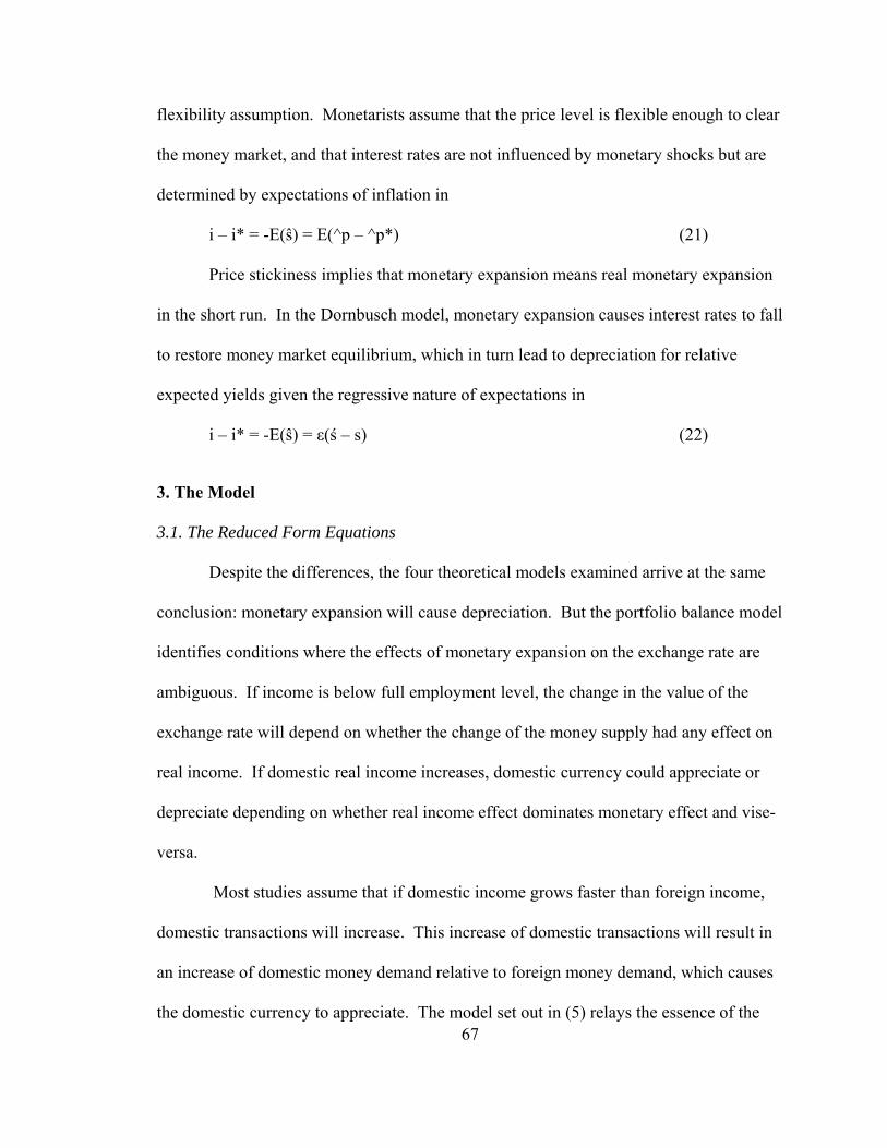
67
flexibility assumption. Monetarists assume that the price level is flexible enough to clear
the money market, and that interest rates are not influenced by monetary shocks but are
determined by expectations of inflation in
i – i* = -E(ŝ) = E(^p – ^p*) (21)
Price stickiness implies that monetary expansion means real monetary expansion
in the short run. In the Dornbusch model, monetary expansion causes interest rates to fall
to restore money market equilibrium, which in turn lead to depreciation for relative
expected yields given the regressive nature of expectations in
i – i* = -E(ŝ) = ε(ś – s) (22)
3. The Model
3.1. The Reduced Form Equations
Despite the differences, the four theoretical models examined arrive at the same
conclusion: monetary expansion will cause depreciation. But the portfolio balance model
identifies conditions where the effects of monetary expansion on the exchange rate are
ambiguous. If income is below full employment level, the change in the value of the
exchange rate will depend on whether the change of the money supply had any effect on
real income. If domestic real income increases, domestic currency could appreciate or
depreciate depending on whether real income effect dominates monetary effect and vise-
versa.
Most studies assume that if domestic income grows faster than foreign income,
domestic transactions will increase. This increase of domestic transactions will result in
an increase of domestic money demand relative to foreign money demand, which causes
the domestic currency to appreciate. The model set out in (5) relays the essence of the
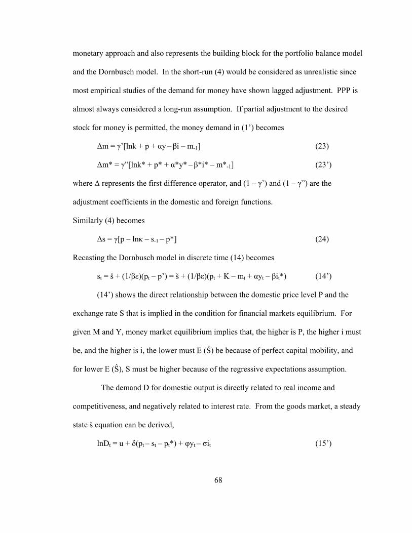
68
monetary approach and also represents the building block for the portfolio balance model
and the Dornbusch model. In the short-run (4) would be considered as unrealistic since
most empirical studies of the demand for money have shown lagged adjustment. PPP is
almost always considered a long-run assumption. If partial adjustment to the desired
stock for money is permitted, the money demand in (1’) becomes
∆m = γ’[lnk + p + αy – βi – m-1] (23)
∆m* = γ”[lnk* + p* + α*y* – β*i* – m*-1] (23’)
where ∆ represents the first difference operator, and (1 – γ’) and (1 – γ”) are the
adjustment coefficients in the domestic and foreign functions.
Similarly (4) becomes
∆s = γ[p – lnκ – s-1 – p*] (24)
Recasting the Dornbusch model in discrete time (14) becomes
st = š + (1/βε)(pt – p’) = š + (1/βε)(pt + K – mt + αyt – βit*) (14’)
(14’) shows the direct relationship between the domestic price level P and the
exchange rate S that is implied in the condition for financial markets equilibrium. For
given M and Y, money market equilibrium implies that, the higher is P, the higher i must
be, and the higher is i, the lower must E (Ŝ) be because of perfect capital mobility, and
for lower E (Ŝ), S must be higher because of the regressive expectations assumption.
The demand D for domestic output is directly related to real income and
competitiveness, and negatively related to interest rate. From the goods market, a steady
state š equation can be derived,
lnDt = u + δ(pt – st – pt*) + φyt – σit (15’)
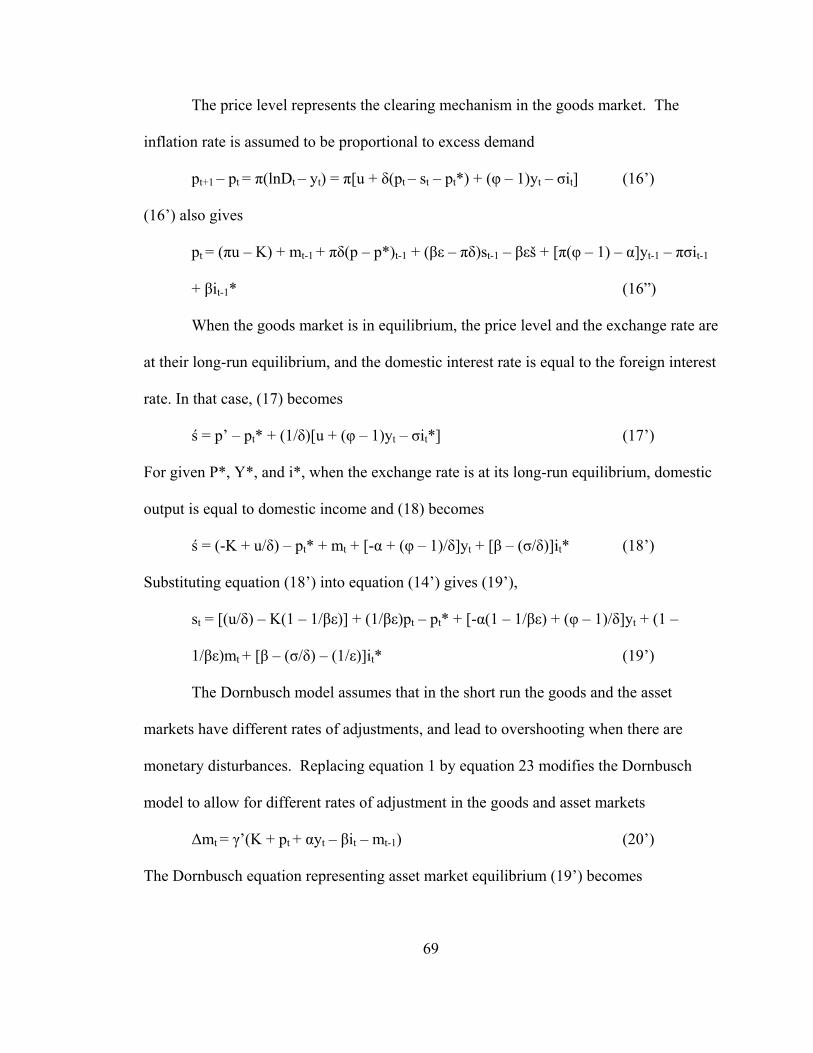
69
The price level represents the clearing mechanism in the goods market. The
inflation rate is assumed to be proportional to excess demand
pt+1 – pt = π(lnDt – yt) = π[u + δ(pt – st – pt*) + (φ – 1)yt – σit] (16’)
(16’) also gives
pt = (πu – K) + mt-1 + πδ(p – p*)t-1 + (βε – πδ)st-1 – βεš + [π(φ – 1) – α]yt-1 – πσit-1
+ βit-1* (16”)
When the goods market is in equilibrium, the price level and the exchange rate are
at their long-run equilibrium, and the domestic interest rate is equal to the foreign interest
rate. In that case, (17) becomes
ś = p’ – pt* + (1/δ)[u + (φ – 1)yt – σit*] (17’)
For given P*, Y*, and i*, when the exchange rate is at its long-run equilibrium, domestic
output is equal to domestic income and (18) becomes
ś = (-K + u/δ) – pt* + mt + [-α + (φ – 1)/δ]yt + [β – (σ/δ)]it* (18’)
Substituting equation (18’) into equation (14’) gives (19’),
st = [(u/δ) – K(1 – 1/βε)] + (1/βε)pt – pt* + [-α(1 – 1/βε) + (φ – 1)/δ]yt + (1 –
1/βε)mt + [β – (σ/δ) – (1/ε)]it* (19’)
The Dornbusch model assumes that in the short run the goods and the asset
markets have different rates of adjustments, and lead to overshooting when there are
monetary disturbances. Replacing equation 1 by equation 23 modifies the Dornbusch
model to allow for different rates of adjustment in the goods and asset markets
∆mt = γ’(K + pt + αyt – βit – mt-1) (20’)
The Dornbusch equation representing asset market equilibrium (19’) becomes
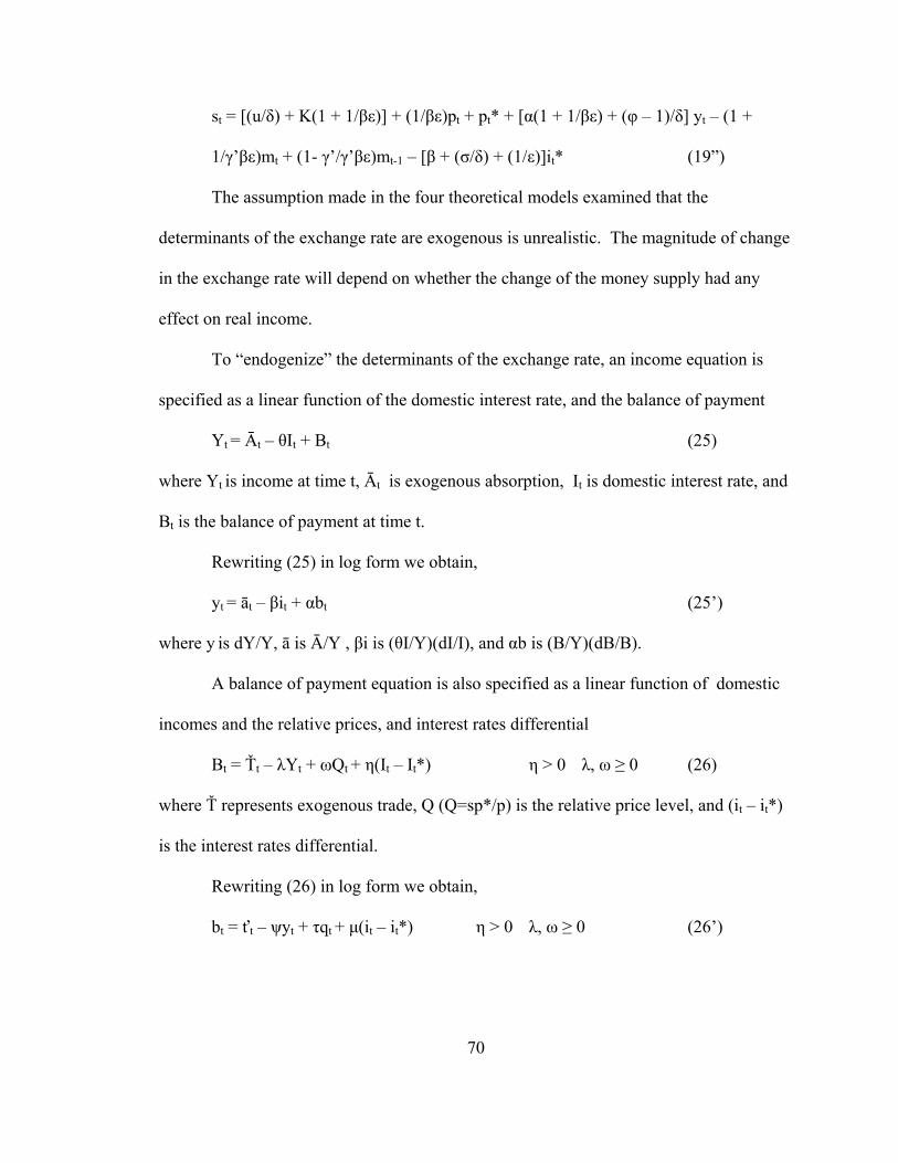
70
st = [(u/δ) + K(1 + 1/βε)] + (1/βε)pt + pt* + [α(1 + 1/βε) + (φ – 1)/δ] yt – (1 +
1/γ’βε)mt + (1- γ’/γ’βε)mt-1 – [β + (σ/δ) + (1/ε)]it* (19”)
The assumption made in the four theoretical models examined that the
determinants of the exchange rate are exogenous is unrealistic. The magnitude of change
in the exchange rate will depend on whether the change of the money supply had any
effect on real income.
To “endogenize” the determinants of the exchange rate, an income equation is
specified as a linear function of the domestic interest rate, and the balance of payment
Yt = Āt – θIt + Bt (25)
where Yt is income at time t, Āt is exogenous absorption, It is domestic interest rate, and
Bt is the balance of payment at time t.
Rewriting (25) in log form we obtain,
yt = āt – βit + αbt (25’)
where y is dY/Y, ā is Ā/Y , βi is (θI/Y)(dI/I), and αb is (B/Y)(dB/B).
A balance of payment equation is also specified as a linear function of domestic
incomes and the relative prices, and interest rates differential
Bt = Ťt – λYt + ωQt + η(It – It*) η > 0 λ, ω ≥ 0 (26)
where Ť represents exogenous trade, Q (Q=sp*/p) is the relative price level, and (it – it*)
is the interest rates differential.
Rewriting (26) in log form we obtain,
bt = ťt – ψyt + τqt + µ(it – it*) η > 0 λ, ω ≥ 0 (26’)
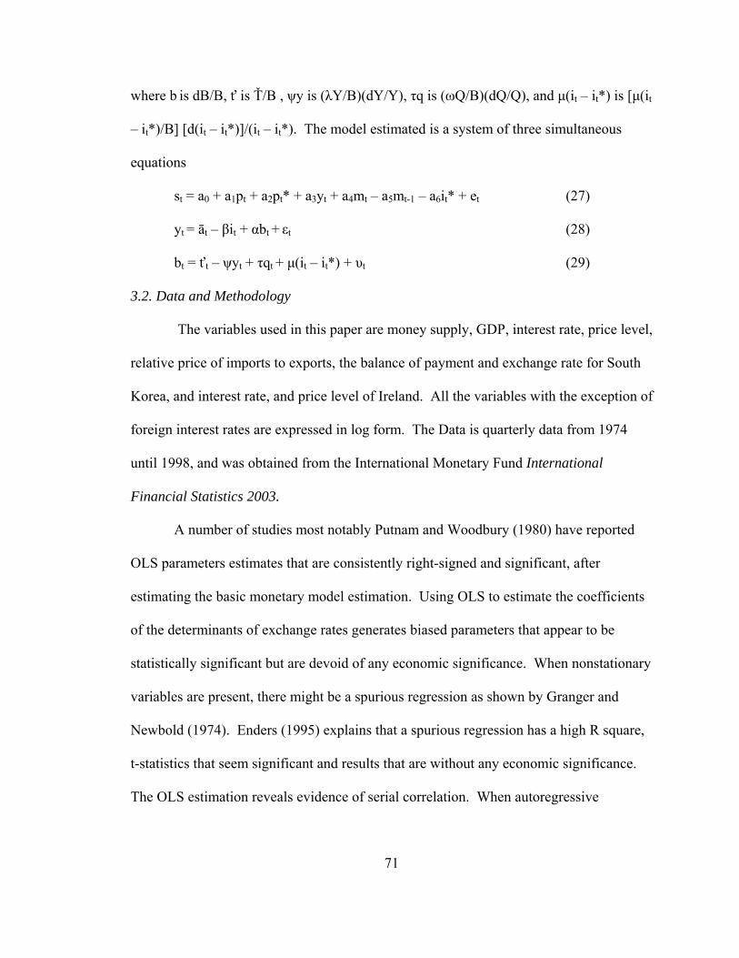
71
where b is dB/B, ť is Ť/B , ψy is (λY/B)(dY/Y), τq is (ωQ/B)(dQ/Q), and µ(it – it*) is [µ(it
– it*)/B] [d(it – it*)]/(it – it*). The model estimated is a system of three simultaneous
equations
st = a0 + a1pt + a2pt* + a3yt + a4mt – a5mt-1 – a6it* + et (27)
yt = āt – βit + αbt + εt (28)
bt = ťt – ψyt + τqt + µ(it – it*) + υt (29)
3.2. Data and Methodology
The variables used in this paper are money supply, GDP, interest rate, price level,
relative price of imports to exports, the balance of payment and exchange rate for South
Korea, and interest rate, and price level of Ireland. All the variables with the exception of
foreign interest rates are expressed in log form. The Data is quarterly data from 1974
until 1998, and was obtained from the International Monetary Fund International
Financial Statistics 2003.
A number of studies most notably Putnam and Woodbury (1980) have reported
OLS parameters estimates that are consistently right-signed and significant, after
estimating the basic monetary model estimation. Using OLS to estimate the coefficients
of the determinants of exchange rates generates biased parameters that appear to be
statistically significant but are devoid of any economic significance. When nonstationary
variables are present, there might be a spurious regression as shown by Granger and
Newbold (1974). Enders (1995) explains that a spurious regression has a high R square,
t-statistics that seem significant and results that are without any economic significance.
The OLS estimation reveals evidence of serial correlation. When autoregressive
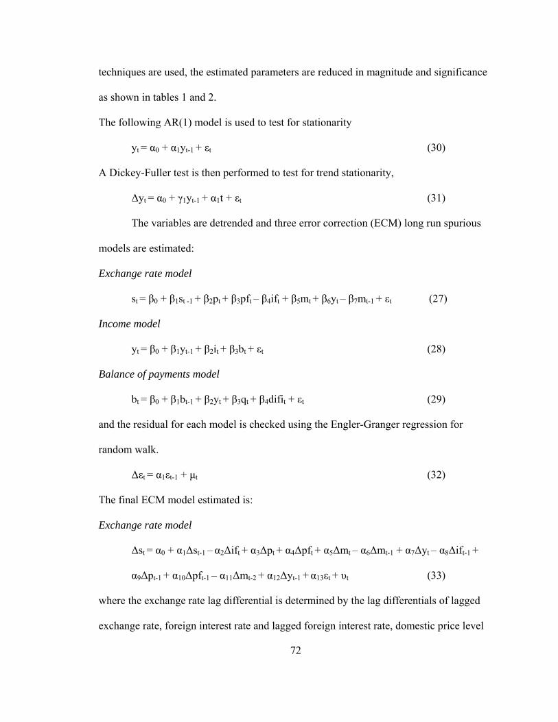
72
techniques are used, the estimated parameters are reduced in magnitude and significance
as shown in tables 1 and 2.
The following AR(1) model is used to test for stationarity
yt = α0 + α1yt-1 + εt (30)
A Dickey-Fuller test is then performed to test for trend stationarity,
∆yt = α0 + γ1yt-1 + α1t + εt (31)
The variables are detrended and three error correction (ECM) long run spurious
models are estimated:
Exchange rate model
st = β0 + β1st -1 + β2pt + β3pft – β4ift + β5mt + β6yt – β7mt-1 + εt (27)
Income model
yt = β0 + β1yt-1 + β2it + β3bt + εt (28)
Balance of payments model
bt = β0 + β1bt-1 + β2yt + β3qt + β4difit + εt (29)
and the residual for each model is checked using the Engler-Granger regression for
random walk.
∆εt = α1εt-1 + µt (32)
The final ECM model estimated is:
Exchange rate model
∆st = α0 + α1∆st-1 – α2∆ift + α3∆pt + α4∆pft + α5∆mt – α6∆mt-1 + α7∆yt – α8∆ift-1 +
α9∆pt-1 + α10∆pft-1 – α11∆mt-2 + α12∆yt-1 + α13εt + υt (33)
where the exchange rate lag differential is determined by the lag differentials of lagged
exchange rate, foreign interest rate and lagged foreign interest rate, domestic price level
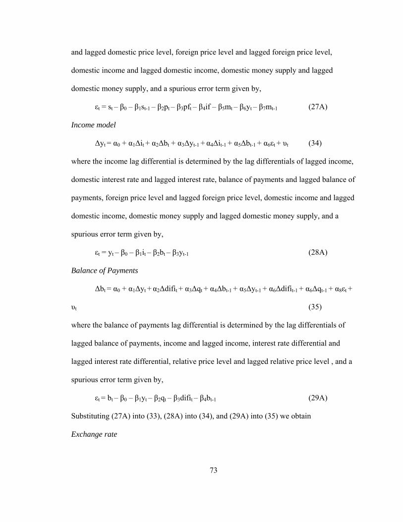
73
and lagged domestic price level, foreign price level and lagged foreign price level,
domestic income and lagged domestic income, domestic money supply and lagged
domestic money supply, and a spurious error term given by,
εt = st – β0 – β1st-1 – β2pt – β3pft – β4if – β5mt – β6yt – β7mt-1 (27A)
Income model
∆yt = α0 + α1∆it + α2∆bt + α3∆yt-1 + α4∆it-1 + α5∆bt-1 + α6εt + υt (34)
where the income lag differential is determined by the lag differentials of lagged income,
domestic interest rate and lagged interest rate, balance of payments and lagged balance of
payments, foreign price level and lagged foreign price level, domestic income and lagged
domestic income, domestic money supply and lagged domestic money supply, and a
spurious error term given by,
εt = yt – β0 – β1it – β2bt – β3yt-1 (28A)
Balance of Payments
∆bt = α0 + α1∆yt + α2∆difit + α3∆qt + α4∆bt-1 + α5∆yt-1 + α6∆difit-1 + α6∆qt-1 + α8εt +
υt (35)
where the balance of payments lag differential is determined by the lag differentials of
lagged balance of payments, income and lagged income, interest rate differential and
lagged interest rate differential, relative price level and lagged relative price level , and a
spurious error term given by,
εt = bt – β0 – β1yt – β2qt – β3difit – β4bt-1 (29A)
Substituting (27A) into (33), (28A) into (34), and (29A) into (35) we obtain
Exchange rate
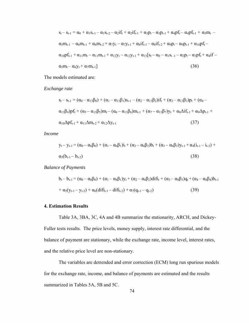
74
st – st-1 = α0 + α1st-1 – α1st-2 – α2ift + α2ift-1 + α3pt – α3pt-1 + α4pft – α4pft-1 + α5mt –
α5mt-1 – α6mt-1 + α6mt-2 + α7yt – α7yt-1 + α8ift-1 – α8ift-2 + α9pt – α9pt-1 + α10pft –
α10pft-1 + α11mt – α11mt-1 + α12yt – α12yt-1 + α13[st – α0 – α1st -1 – α2pt – α3pft + α4if –
α5mt – α6yt + α7mt-1] (36)
The models estimated are:
Exchange rate
st – st-1 = (α0 – α13β0) + (α1 – α13β1)st-1 – (α2 – α13β2)ift + (α3 – α13β3)pt + (α4 –
α13β4)pft + (α5 – α13β5)mt – (α6 – α13β6)mt-1 + (α7 – α13β7)yt + α8∆ift-1 + α9∆pt-1 +
α10∆pft-1 + α11∆mt-2 + α12∆yt-1 (37)
Income
yt – yt-1 = (α0 – α6β0) + (α1 – α6β1)it + (α2 – α6β2)bt + (α3 – α6β3)yt-1 + α4(it-1 – it-2) +
α5(bt-1 – bt-2) (38)
Balance of Payments
bt – bt-1 = (α0 – α8β0) + (α1 – α8β1)yt + (α2 – α8β2)difit + (α3 – α8β3)qt + (α4 – α8β4)bt-1
+ α5(yt-1 – yt-2) + α6(difit-1 – difit-2) + α7(qt-1 – qt-2) (39)
4. Estimation Results
Table 3A, 3BA, 3C, 4A and 4B summarize the stationarity, ARCH, and Dickey-
Fuller tests results. The price levels, money supply, interest rate differential, and the
balance of payment are stationary, while the exchange rate, income level, interest rates,
and the relative price level are non-stationary.
The variables are detrended and error correction (ECM) long run spurious models
for the exchange rate, income, and balance of payments are estimated and the results
summarized in Tables 5A, 5B and 5C.
75
To account for endogeneity, a three stage least square (3SLS) regression is used to
estimate the coefficients of the determinants of exchange rate, income, and balance of
payments. The estimated exchange rate coefficients are shown in Table 6A.
4.1. The Exchange Rate Estimation Results
The lagged exchange rate coefficient is -0.99 almost unit value and is significant
at 99% level, implying that any change in the exchange rate at time t-1 period, ceteris
paribus, is reversed at time t. An appreciation of the currency in period one is followed
by an equal depreciation the following period, elimination any change in the value of the
currency.
Foreign interest rates are not significant. The Korean government restricted the
movement of capital, especially the outflow of Korean capital. High foreign interest rates
were not sufficient to attract Korean capital. High foreign interest rates did not affect the
exchange rate since Koreans were not able to invest abroad.
The negative sign of domestic price level coefficient is inconsistent with PPP and
is statistically significant at 95% level. The negative sign of the price level could be due
to price stickiness, consistent with the Dornbusch model. For a given level of output, the
Dornbusch model states that following a monetary expansion, the exchange rate will
overshoot its long-run equilibrium due to the rigidity of the price level. The subsequent
adjustment process will lead to appreciation and rising prices.
The exchange rate elasticity with respect to the price level is -0.27, implying a
10% increase in prices will cause a 2.7% appreciation in the currency. According to PPP,
an increase in the price level causes the currency to depreciate. Rivera-Batiz and Rivera-
Batiz explain that from time to time PPP fail to explain exchange rate changes. Between
76
1981 and 1985, if PPP were to hold, the dollar should have depreciated when it
persistently appreciated in value.
The two periods lagged change in money supply is statistically significant at the
90% level and has negative sign implying appreciation. The opposite signs of the money
supply and the two periods lagged change in the money supply support the overshooting
assumption of the Dornbusch model. A 10% increase in the money supply will cause the
currency to depreciate at first, overshooting its long-run equilibrium, and then to revert to
its long-run equilibrium. Two periods after a 10% increase in the money supply, the
currency appreciates by 4.2%.
The signs of the coefficients of income and lagged change in income are negative
and consistent with the theory. A 10% increase in income will cause 2.8% appreciation.
Rising incomes lead to an increase in domestic transactions. This higher rate of domestic
transactions results in a higher money demand relative to foreign money demand which
causes appreciation.
4.2. The Income Estimation Results
The coefficients of income are reported in Table 6B. With the exception of the
intercept and interest rate, all the parameters are insignificant. The intercept represents
autonomous absorption such as government spending, and is statistically significant at the
99% level. The coefficient value is zero implying the government spending does not
contribute to income.
The interest rate coefficient is positive and significant at 99% level. The sign of
interest rate is contrary to expectation, and implies that a 1% increase in interest rate will
77
lead to a 0.28% increase in income. The increase in income could be caused by an
inflow foreign capital.
4.3. The Balance of Payments Estimation Results
The balance of payments estimates are reported in Table 6C. The lagged balance
of payments coefficient is significant at the 99% level and negative, implying that a 10%
balance of payment “surplus” will lead to 3.83% balance of payment deficit the following
period. A BOP surplus represents an inflow of funds and an increase in the money
supply. The expanding money supply will cause the relative price level to change,
making export expensive and imports less expensive. The change in the relative price
level leads to a BOP deficit.
The income coefficient is also significant at the 99% level and negative. The
income coefficient represents the marginal propensity to import; a 10% increase in
income will increase in the balance of payments deficit by 20%.
The coefficient of the lagged change in income is also negative and significant at
the 99% level. All the other variables are not significant.
5. Conclusion
The model estimated shows that the BOP curve for Korea lies below the LM
curve, implying that capital is responsive to interest rate changes. Although Korea
restricts the movement of domestic capital, it has been able to attract foreign capital. As
Korean income increases, ceteris paribus, the Korean won appreciates. The model also
shows that as income increases, the balance of payment deteriorates. As Koreans become
wealthier their consumption of imports increases. The model can be extended to other
countries in estimating the change in the value of a country’s currency relative to that of a
78
trading partner. The treatment of capital by countries adopting export-led growth policies
is detrimental to the efficacy of that strategy. Countries relying on exports to fuel their
economic growth want to keep the value of their currency inelastic relative to income.
The model endogenizes the determinants of the exchange rate, income, and the balance of
payments, and predicts the effect of economic growth on the exchange rate, and the
changes in the exchange rate on the balance of payments and income.
In future research, I will include the relative money supply, income, interest rate, price
level, and balance of payments of two trading partners in estimating the exchange rate.
Including variables from both countries may yield more robust results.
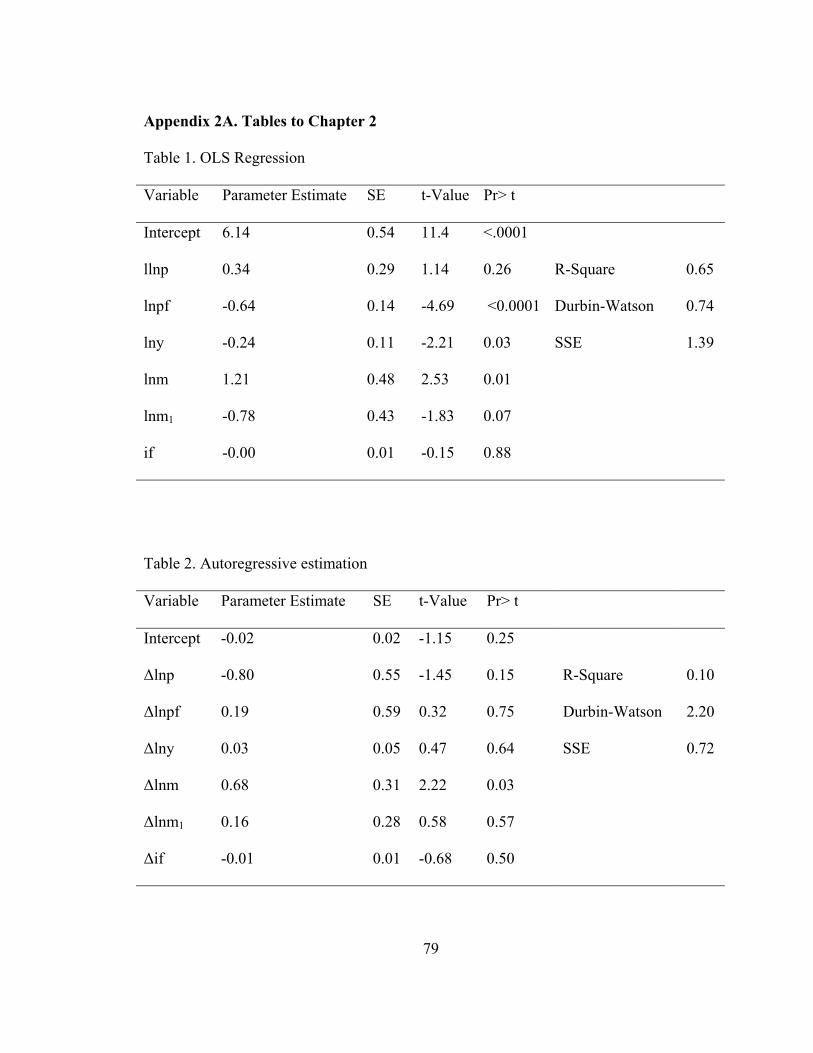
79
Appendix 2A. Tables to Chapter 2
Table 1. OLS Regression
Variable Parameter Estimate SE t-Value Pr> t
Intercept 6.14 0.54 11.4 <.0001
llnp 0.34 0.29 1.14 0.26 R-Square 0.65
lnpf -0.64 0.14 -4.69 <0.0001 Durbin-Watson 0.74
lny -0.24 0.11 -2.21 0.03 SSE 1.39
lnm 1.21 0.48 2.53 0.01
lnm1 -0.78 0.43 -1.83 0.07
if -0.00 0.01 -0.15 0.88
Table 2. Autoregressive estimation
Variable Parameter Estimate SE t-Value Pr> t
Intercept -0.02 0.02 -1.15 0.25
∆lnp -0.80 0.55 -1.45 0.15 R-Square 0.10
∆lnpf 0.19 0.59 0.32 0.75 Durbin-Watson 2.20
∆lny 0.03 0.05 0.47 0.64 SSE 0.72
∆lnm 0.68 0.31 2.22 0.03
∆lnm1 0.16 0.28 0.58 0.57
∆if -0.01 0.01 -0.68 0.50
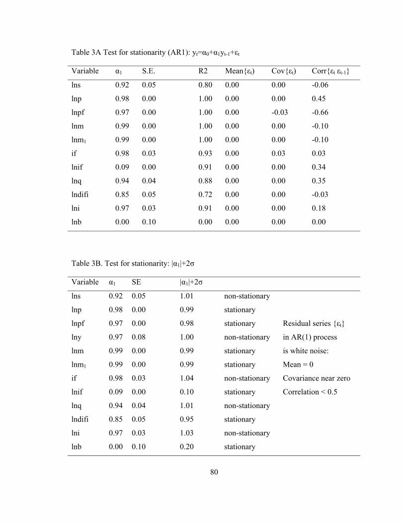
80
Table 3A Test for stationarity (AR1): yt=α0+α1yt-1+εt
Variable α1 S.E. R2 Mean{εt) Cov{εt) Corr{εt εt-1}
lns 0.92 0.05 0.80 0.00 0.00 -0.06
lnp 0.98 0.00 1.00 0.00 0.00 0.45
lnpf 0.97 0.00 1.00 0.00 -0.03 -0.66
lnm 0.99 0.00 1.00 0.00 0.00 -0.10
lnm1 0.99 0.00 1.00 0.00 0.00 -0.10
if 0.98 0.03 0.93 0.00 0.03 0.03
lnif 0.09 0.00 0.91 0.00 0.00 0.34
lnq 0.94 0.04 0.88 0.00 0.00 0.35
lndifi 0.85 0.05 0.72 0.00 0.00 -0.03
lni 0.97 0.03 0.91 0.00 0.00 0.18
lnb 0.00 0.10 0.00 0.00 0.00 0.00
Table 3B. Test for stationarity: |α1|+2σ
Variable α1 SE |α1|+2σ
lns 0.92 0.05 1.01 non-stationary
lnp 0.98 0.00 0.99 stationary
lnpf 0.97 0.00 0.98 stationary Residual series {εt}
lny 0.97 0.08 1.00 non-stationary in AR(1) process
lnm 0.99 0.00 0.99 stationary is white noise:
lnm1 0.99 0.00 0.99 stationary Mean = 0
if 0.98 0.03 1.04 non-stationary Covariance near zero
lnif 0.09 0.00 0.10 stationary Correlation < 0.5
lnq 0.94 0.04 1.01 non-stationary
lndifi 0.85 0.05 0.95 stationary
lni 0.97 0.03 1.03 non-stationary
lnb 0.00 0.10 0.20 stationary
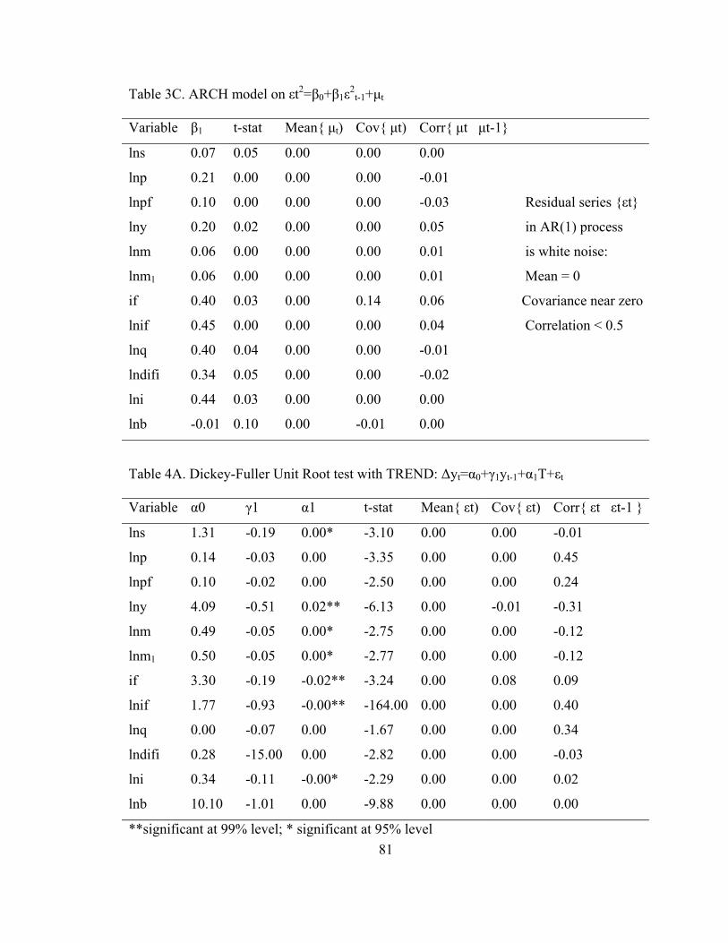
81
Table 3C. ARCH model on εt2=β0+β1ε2t-1+µt
Variable β1 t-stat Mean{ µt) Cov{ µt) Corr{ µt µt-1}
lns 0.07 0.05 0.00 0.00 0.00
lnp 0.21 0.00 0.00 0.00 -0.01
lnpf 0.10 0.00 0.00 0.00 -0.03 Residual series {εt}
lny 0.20 0.02 0.00 0.00 0.05 in AR(1) process
lnm 0.06 0.00 0.00 0.00 0.01 is white noise:
lnm1 0.06 0.00 0.00 0.00 0.01 Mean = 0
if 0.40 0.03 0.00 0.14 0.06 Covariance near zero
lnif 0.45 0.00 0.00 0.00 0.04 Correlation < 0.5
lnq 0.40 0.04 0.00 0.00 -0.01
lndifi 0.34 0.05 0.00 0.00 -0.02
lni 0.44 0.03 0.00 0.00 0.00
lnb -0.01 0.10 0.00 -0.01 0.00
Table 4A. Dickey-Fuller Unit Root test with TREND: ∆yt=α0+γ1yt-1+α1T+εt
Variable α0 γ1 α1 t-stat Mean{ εt) Cov{ εt) Corr{ εt εt-1 }
lns 1.31 -0.19 0.00* -3.10 0.00 0.00 -0.01
lnp 0.14 -0.03 0.00 -3.35 0.00 0.00 0.45
lnpf 0.10 -0.02 0.00 -2.50 0.00 0.00 0.24
lny 4.09 -0.51 0.02** -6.13 0.00 -0.01 -0.31
lnm 0.49 -0.05 0.00* -2.75 0.00 0.00 -0.12
lnm1 0.50 -0.05 0.00* -2.77 0.00 0.00 -0.12
if 3.30 -0.19 -0.02** -3.24 0.00 0.08 0.09
lnif 1.77 -0.93 -0.00** -164.00 0.00 0.00 0.40
lnq 0.00 -0.07 0.00 -1.67 0.00 0.00 0.34
lndifi 0.28 -15.00 0.00 -2.82 0.00 0.00 -0.03
lni 0.34 -0.11 -0.00* -2.29 0.00 0.00 0.02
lnb 10.10 -1.01 0.00 -9.88 0.00 0.00 0.00
**significant at 99% level; * significant at 95% level
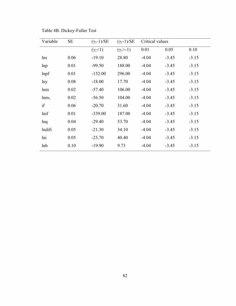
82
Table 4B. Dickey-Fuller Test
Variable SE (γ1-1)/SE (γ1-1)/SE Critical values
(γ1<1) (γ1>-1) 0.01 0.05 0.10
lns 0.06 -19.10 28.80 -4.04 -3.45 -3.15
lnp 0.01 -99.50 188.00 -4.04 -3.45 -3.15
lnpf 0.01 -152.00 296.00 -4.04 -3.45 -3.15
lny 0.08 -18.00 17.70 -4.04 -3.45 -3.15
lnm 0.02 -57.40 106.00 -4.04 -3.45 -3.15
lnm1 0.02 -56.50 104.00 -4.04 -3.45 -3.15
if 0.06 -20.70 31.60 -4.04 -3.45 -3.15
lnif 0.01 -339.00 187.00 -4.04 -3.45 -3.15
lnq 0.04 -29.40 53.70 -4.04 -3.45 -3.15
lndifi 0.05 -21.30 34.10 -4.04 -3.45 -3.15
lni 0.05 -23.70 40.40 -4.04 -3.45 -3.15
lnb 0.10 -19.90 9.73 -4.04 -3.45 -3.15
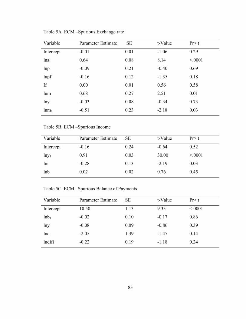
83
Table 5A. ECM –Spurious Exchange rate
Variable Parameter Estimate SE t-Value Pr> t
Intercept -0.01 0.01 -1.06 0.29
lns1 0.64 0.08 8.14 <.0001
lnp -0.09 0.21 -0.40 0.69
lnpf -0.16 0.12 -1.35 0.18
If 0.00 0.01 0.56 0.58
lnm 0.68 0.27 2.51 0.01
lny -0.03 0.08 -0.34 0.73
lnm1 -0.51 0.23 -2.18 0.03
Table 5B. ECM –Spurious Income
Variable Parameter Estimate SE t-Value Pr> t
Intercept -0.16 0.24 -0.64 0.52
lny1 0.91 0.03 30.00 <.0001
lni -0.28 0.13 -2.19 0.03
lnb 0.02 0.02 0.76 0.45
Table 5C. ECM –Spurious Balance of Payments
Variable Parameter Estimate SE t-Value Pr> t
Intercept 10.50 1.13 9.33 <.0001
lnb1 -0.02 0.10 -0.17 0.86
lny -0.08 0.09 -0.86 0.39
lnq -2.05 1.39 -1.47 0.14
lndifi -0.22 0.19 -1.18 0.24
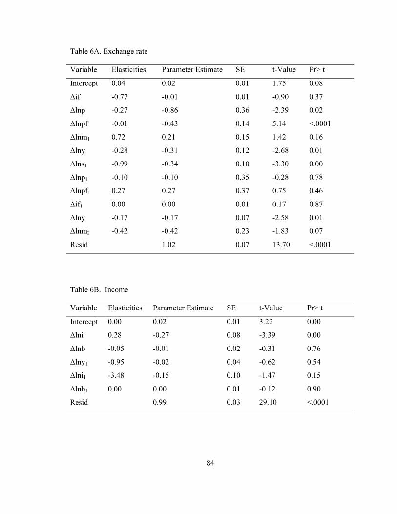
84
Table 6A. Exchange rate
Variable Elasticities Parameter Estimate SE t-Value Pr> t
Intercept 0.04 0.02 0.01 1.75 0.08
∆if -0.77 -0.01 0.01 -0.90 0.37
∆lnp -0.27 -0.86 0.36 -2.39 0.02
∆lnpf -0.01 -0.43 0.14 5.14 <.0001
∆lnm1 0.72 0.21 0.15 1.42 0.16
∆lny -0.28 -0.31 0.12 -2.68 0.01
∆lns1 -0.99 -0.34 0.10 -3.30 0.00
∆lnp1 -0.10 -0.10 0.35 -0.28 0.78
∆lnpf1 0.27 0.27 0.37 0.75 0.46
∆if1 0.00 0.00 0.01 0.17 0.87
∆lny -0.17 -0.17 0.07 -2.58 0.01
∆lnm2 -0.42 -0.42 0.23 -1.83 0.07
Resid 1.02 0.07 13.70 <.0001
Table 6B. Income
Variable Elasticities Parameter Estimate SE t-Value Pr> t
Intercept 0.00 0.02 0.01 3.22 0.00
∆lni 0.28 -0.27 0.08 -3.39 0.00
∆lnb -0.05 -0.01 0.02 -0.31 0.76
∆lny1 -0.95 -0.02 0.04 -0.62 0.54
∆lni1 -3.48 -0.15 0.10 -1.47 0.15
∆lnb1 0.00 0.00 0.01 -0.12 0.90
Resid 0.99 0.03 29.10 <.0001
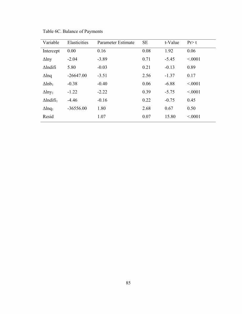
85
Table 6C. Balance of Payments
Variable Elasticities Parameter Estimate SE t-Value Pr> t
Intercept 0.00 0.16 0.08 1.92 0.06
∆lny -2.04 -3.89 0.71 -5.45 <.0001
∆lndifi 5.80 -0.03 0.21 -0.13 0.89
∆lnq -26647.00 -3.51 2.56 -1.37 0.17
∆lnb1 -0.38 -0.40 0.06 -6.88 <.0001
∆lny1 -1.22 -2.22 0.39 -5.75 <.0001
∆lndifi1 -4.46 -0.16 0.22 -0.75 0.45
∆lnq1 -36556.00 1.80 2.68 0.67 0.50
Resid 1.07 0.07 15.80 <.0001
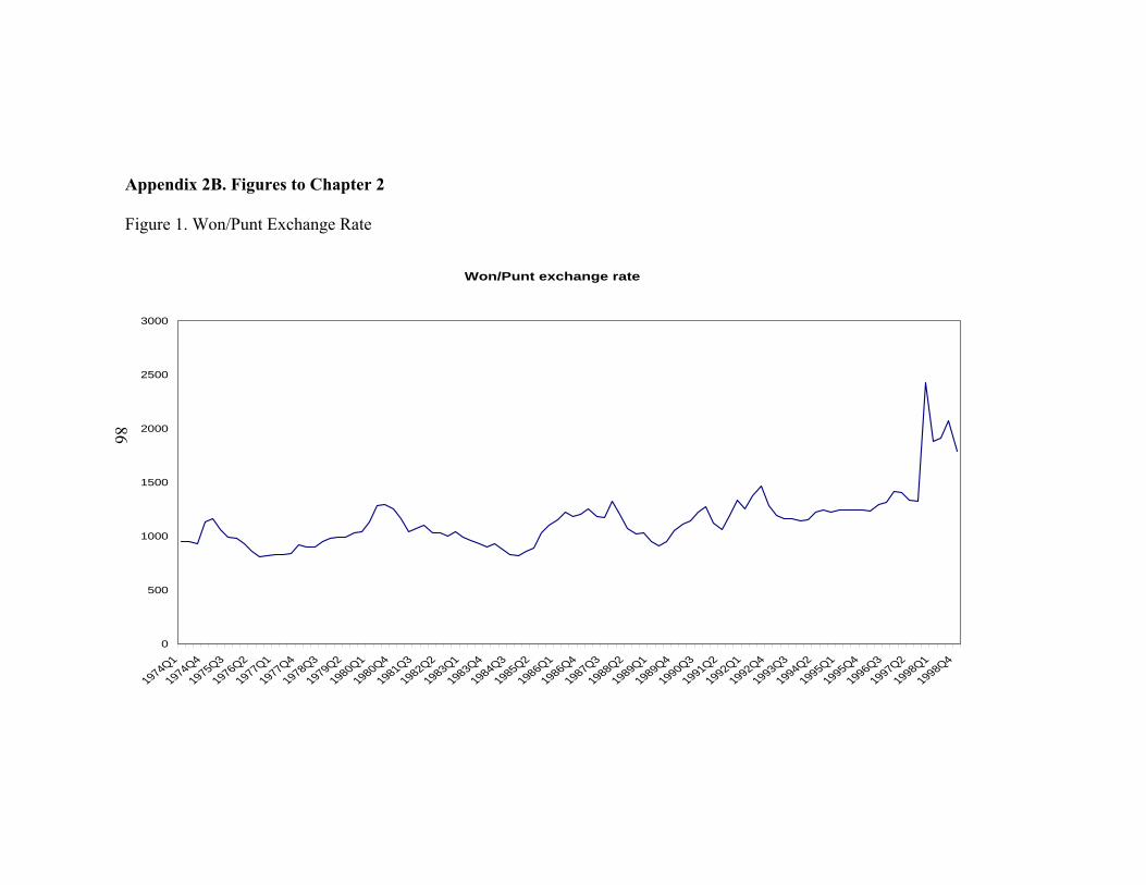
Appendix 2B. Figures to Chapter 2
Figure 1. Won/Punt Exchange Rate
86
Won/Punt exchange rate
0
500
1000
1500
2000
2500
3000
1974Q11974Q41975Q31976Q21977Q11977Q41978Q31979Q21980Q11980Q41981Q31982Q21983Q11983Q41984Q31985Q21986Q11986Q41987Q31988Q21989Q11989Q41990Q31991Q21992Q11992Q41993Q31994Q21995Q11995Q41996Q31997Q21998Q11998Q4
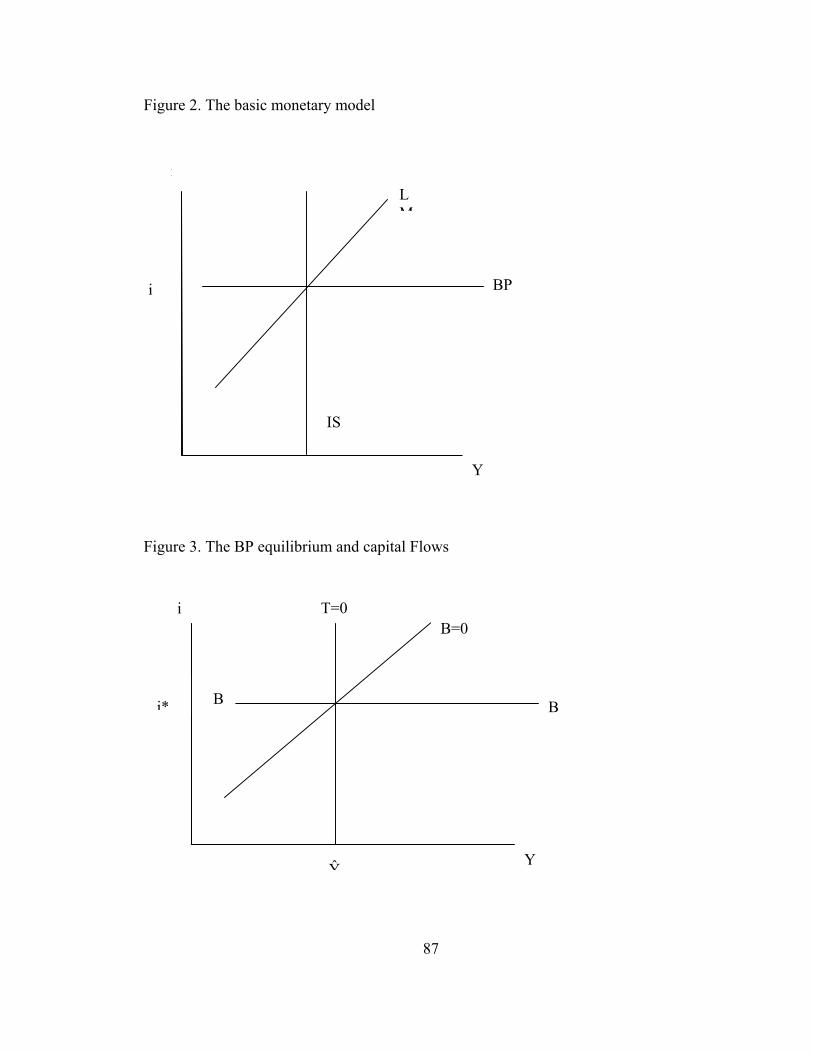
Figure 2. The basic monetary model
iLM
87
Figure 3. The BP equilibrium and capital Flows
IS
BP
Y
i
i
Ŷ
B=0T=0
B i*
B
Y
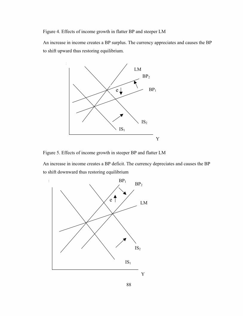
Figure 4. Effects of income growth in flatter BP and steeper LM
An increase in income creates a BP surplus. The currency appreciates and causes the BP
to shift upward thus restoring equilibrium.
BP1
BP2
LM i
Figure 5. Effects of income growth
An increase in income creates a BP
to shift downward thus restoring eq
e
i
e
IS2
Y
IS1
in steeper BP and flatter LM
deficit. The currency depreciates and causes the BP
uilibrium
BP2
BP1
LM
IS2
Y
IS1
88
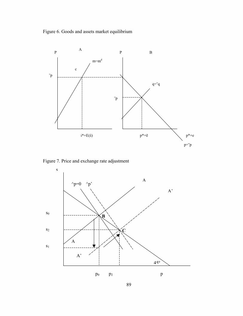
Figure 6. Goods and assets market equilibrium
c
BA
m=md
P
⎯p
q=⎯q
i*+E(ŝ) p*+ē p*+e p=⎯p
⎯p
P
Figure 7. Price and exchange rate adjustment
s0
s2 s1
A’
A
A
^p=0 ^p’
45ºA’
B
C
s
p0 p2 p
89
90
BIBLIOGRAPHY
Allen, R.G.D. (1938). Mathematical Analysis for Economists. New York: MacMillan.
Alonso-Gamo, P., Fennell, S., & Sakr, K. (1997). Adjusting to New Realities: MENA,
The Uruguay Round, and the EU-Mediterranean Initiative. IMF Working Paper.
Balassa, B. (1964). The Purchasing-Power Parity Doctrine: A Reappraisal. The Journal
of Political Economy, Vol. 72, No. 6. 584-596.
Barro, R. J. (1990). Government Spending in a Simple Model of Endogenous Growth.
Journal of Political Economy 98: S103-S126.
Bilson, J. (1978). The Current Experience with Floating Exchange Rates: An Appraisal
of the Monetary Approach. The American Economic Review, Vol. 68, No. 2,
Papers and Proceedings of the Ninetieth Annual Meeting of the American
Economic Association 392-397.
Branson, W.H. & Haltunen, H. (1979). Asset-Market Determination of Exchange Rates:
Initial Empirical and Policy Results. In Trade and Payments Adjustment Under
Flexible Exchange rates. Edited by J.P. Martin and A. Smith, Macmillan.
Branson, W.H. (1986). The Limits of Monetary Coordination as Exchange rate Policy.
Brookings Papers on Economic Activity, 1986 (1) 175-194.
Brown, D., Kiyota, K. & Stern, R.M. (2004). Computational Analysis of the U.S.
Bilateral Free Trade Agreements with Central America, Australia, and Morocco.
www.fordschool.umich.edu/rsie/seminar/BrownKiyotaStern.pdf
91
Chang, W. (1979). Some Theorems of Trade and General Equilibrium with Many Goods
and Factors. Econometrica 47, 709-726.
Dornbush, R. (1980). Exchange Rate Economics: Where do we stand? Brookings
Papers on Economic Activity, 1980 (1) 143-185+187-205.
Dornbush, R. (1976). Expectations and Exchange rates Dynamics. The Journal of
Political Economy, 84 (6) 1161-1176.
Dornbush, R. (1978). Monetary Policy Under Exchange Rate Flexibility. In Managed
Exchange Rate Flexibility: The Recent Experience. Federal Reserve bank of
Boston, Conference Series No. 20.
Driskill, R.A. (1976). Exchange-Rate Dynamics: An Empirical Investigation. The
Journal of Political Economy, 89(2)357-371.
Enders, W. (1995). Applied Econometrics Time Series. John Wiley & Sons.
Fels, J. & Grundlach, E. (1990). More Evidence on the Puzzle of Interindustry Wage
Differentials: The case of Wes Germany. Weltwirtschaftliches Archiv, 3, 544-560.
Fleming, J. M. (1962). Domestic Financial Policies Under Fixed and Floating Exchange
Rates. IMF Staff Papers.
Frankel, J.A. (1979). On the Mark: A Theory of Floating Exchange Rates based on Real
Interest Differentials. The American Economic Review, 69 (4) 610-622.
Gilbert, J. (1999). CGE Simulations of US Bilateral Free Trade Agreements.
Background paper prepared for the Free Trade Agreements and US Trade Policy
Conference, Institute For International Economics, Washington, D.C.
Granger, C. & Newbold, P. (1974). Spurious Regressions in Econometrics. Journal of
Econometrics 2, 111-120.
92
Grossman, G.M, & Levinsohn, J.A. (1989). Import Competition and the Stock Market
Return to Capital. American Economic Review, 79 (5), 1065-1087
Hacche, G. & Townend, J. (1981). Exchange Rate and Monetary Policy: Modelling
Sterling’s Effective Exchange rate, 1972-1980. Oxford Economic Papers New
Series, Vol. 33, Supplement: The Money Supply and the Exchange Rate, 201-
247.
Henderson, D.A. (1980). The Dynamic Effects of Exchange market Intervention Policy:
Two Extreme Views and Synthesis. In Economics of flexible Exchange rates.
Edited by Helmut Frish and Gerhard Schwodiauer. Kredit und kapital, Volume 6.
International Monetary Fund. (2003). International Financial Statistics.
International Road Safety News (2005). www. driveandstayalive.com.
Jones, R. & Scheinkman, J. (1977). The Relevance of the Two-Sector Production Model
in Trade Theory. The Journal of Political Economics 15, 65-99.
Jones, R. (1965). The Structure of Simple General Equilibrium Models. Journal of
Political Economy, 557-572.
Karshenas, M. (1994). Structural Adjustment and Employment in the Middle East and
North Africa. Economic Research Forum for the Arab Countries, Iran and
Turkey, Cairo, Egypt. Working Paper 9420.
Katz, L.F & Summers, L.H. (1989). Industry Rents: Evidence and Implications. in
Baily, M.N. and C. Winston, eds, Brookings Papers on Economic Activity:
Microeconomics, 208-275.
Krueger, A.B. & Summers, L.H. (1988). Efficiency Wages and the Inter-industry Wage
Structure. Econometrica, 56, 259-293.
93
Löfgren, H. (1999). Trade Reform and the Poor in Morocco: A Rural-urban General
Equilibrium Analysis of Reduced Protection. TMD Discussion Paper No. 38.
International Food Policy Institute.
McKibbin, W.J. & Sachs, J.D. (1991) Global Linkages. Macroeconomic Interdependence
and Cooperation in the World Economy, Washington, D.C.: The Brookings
Institution.
Mundell, R. A. (1963). Capital Mobility and Stabilisation Policy Under Fixed and
Flexible Exchange Rates. Canadian Journal of Economic and Political Science.
Reprinted in International Economics. Macmillan 1968.
Mussa, M. (1976). The Exchange Rate, The Balance of Payments and Monetary and
Fiscal Policy Under a Regime of Controlled Floating. Scandinavian Journal of
Economics.
Page, J. & Underwood, J. (1997). Growth, the Maghreb, and Free Trade with the
European Union. pp. 98-126 in Galal, Ahmed, and Bernard Hoekman, eds.
Regional Partners in Global Markets: Limits and Possibilities of the Euro-Med
Agreements. Cairo: Centre for Economic Policy Research, London, and Egyptian
Center for Economic Studies.
Putnam, B.H. & Woodbury, J.R. (1980). Exchange Rate Stability and Monetary Policy.
Review of Economic and Business Research 15, 1-10.
Royaume Du Maroc. (2004). Annuaire Statistique. Dirction de la Statistique. Rabat.
Shapouri, S & Rosen, S. (2003). ERS. USDA. Food Security Assessment.
Takayama, A. (1982). On the Theorems of General Competitive Equilibrium of
Production and Trade – A Survey of Some Recent Developments in the Theory of
International Trade. Kieo Economic Studies, 1-37.
94
Thompson, H. (1989). Variable Employment and Income in General Equilibrium.
Southern Economic Journal, 678-683.
Thompson, H. (1995). Factor Intensity Versus Factor Substitution in a Specified General
Equilibrium Model. Journal of Economic Integration, 10 (3): 283-297.
Thompson, H. (1996). NAFTA and Industrial Adjustment: Specific Factor Model of
Production in Alabama. Growth and Change, 3-28.
TradeStats Express (2004). www.tse.export.gov.
United Nations. (2003). COMTRADE database. U.N. Statistical Division, New York,
New York.
United States International Trade Commission. (2004). U.S.-Morocco Free Trade
Agreement: Potential Economywide and Selected Sectoral Effects. USITC
Publication 3704, www. usitc.gov.
USDA. (2003). FAS. Morocco Grain Annual. GAIN Report No. MO3004.
USDA. (2003). FAS. Morocco Grain:New Customs Duties. GAIN Report No.MO3010.