Embed Size (px)
Citation preview

Endogenous Sunk Costs and the Geographic Distribution ofBrand Shares in Consumer Package Goods Industries∗
Bart J. Bronnenberg† Sanjay K. Dhar‡ Jean-Pierre Dubé‡
March 15, 2005Please submit for the Young Economist Award
Abstract
This paper describes industrial market structure in consumer package goods (CPG) in-dustries using a unique database spanning 31 industries and the 50 largest US metropolitanmarkets. In these data, the geographic cross-section of markets accounts for a much largercomponent of a brand’s total share variation than the time-series. Most industries exhibitstriking asymmetries across markets in both a given brand’s market share and the industry’srank-order of shares. Following Sutton’s theory of endogenous sunk costs, a robust set of game-theoretic predictions is generated regarding industrial market structure and the role of brandadvertising. For non-advertising intensive industries, the lower bound on concentration fallsto zero in larger markets. However, concentration is bounded below in advertising-intensiveindustries even as market size grows large. Connected to this finding, we observe an escalationin the level of advertising for larger markets. In contrast, the number of advertised brandsdoes not vary with market size and, consistent with the theory, there does not appear to be anescalation in entry. Nevertheless, we do observe a proliferation in the number of non-advertisedbrands in larger markets. Finally, we collect historic entry dates for two of our industries andfind that order of entry has a strong impact on the rank-order of shares in a market. Thegeographic distribution of entry in these two industries also accounts for spatial clustering,whereby geographically “close” markets exhibit similar market structures. The geographicvariation in historic entry accounts for spatial dependence both in a brand’s share and in itsadvertising intensity. Several alternative explanations for the geographic patterns in our dataare ruled out. In general, the consistency between the patterns in our data and endogenoussunk costs theory suggest a role for advertising in the formation of long-run industrial marketstructure.
keywords: market structure, advertising, order-of-entry, spatial distributionJEL classification: L11, L66, M30, M37, R12
∗We are very grateful to Tim Conley, Matt Gentzkow, Jonathan Levin, Sanjay Sood, Raphael Thomadsen andFlorian Zettelmeyer for insightful comments and discussions. We also thank seminar participants at Cornell Univer-sity, Harvard, MIT, New York University, the University of Chicago, the Yale SOM, the 2004 Choice Symposium inEstes Park, Colorado, the 2004 Marketing Camp at Leuven, and the 2005 NBER Winter I.O. meetings for valuablefeedback and helpful suggestions. We are also grateful to Ed Lebar of Young & Rubicam Brands for providingus with the BAV data, to Jeff Hermann of Nielsen Media Research for the historical advertising data and to thelibrarians of the National Museum of American History for the archival data on coffee. We acknowledge the re-search assistance of Avtar Bhatoey with the collection of the local brand entry data. The second author thanksthe Neubauer faculty fund for research support. The third author acknowledges the support of the Kilts Center forMarketing. All correspondence may be sent to the third author at the University of Chicago, Graduate School ofBusiness, 5807 South Woodlawn Ave, Chicago IL 60637 or via e-mail at [email protected].
†UCLA Anderson Graduate School of Management, University of California, Los Angeles‡Graduate School of Business, University of Chicago
1

1 Introduction
We study geographic patterns in the industrial market structures of consumer package goods
(CPG) industries across US metropolitan markets. In addition to providing a broad description
of market structures, we also provide evidence of how advertising contributes to the formation of
market structures in CPG industries. In the traditional Structure-Conduct-Performance paradigm
(Bain 1956), advertising is treated as an exogenous “Barrier to Entry” that leads to concentrated
market structures and, in turn, reduces competition and raises profits. Empirical findings based
on regressions of industry concentration on advertising have been mixed and, frequently, incon-
clusive (see Bagwell 2003 for a survey of this literature). More generally, the endogeneity of
advertising raises concerns about its use to explain concentration. The recent game-theoretic
literature provides counter-examples in which competition influences the amount of advertising in
an industry and, in turn, the level of concentration. But, the predictions of the theory are often
sensitive to the precise details of the model. One solution is to focus on single industries and
to build fully-specified “structural models” to reflect the exact conduct of firms and consumers.
Alternatively, Sutton (1987, 1991, 2003) focuses on generating a few robust predictions that apply
to a more general set of models. We adopt this latter approach, using a cross-industry analysis
to test predictions about advertising and market structure.
A novel feature of this analysis is the comprehensive database collected to study market
structure in CPG industries. The basic scanner data consist of longitudinal marketing data for
all the brands from 31 CPG industries, covering 39 months in the 50 largest city market areas, as
designated by AC Nielsen. These industries collectively account for about $26 billion in annual
sales revenues. A demographic supplement to these data provides information on households
in each market. For a subset of 23 geographic markets, we match contemporaneous as well as
historic advertising levels from several years prior to the sample. These are measures of media
advertising which, in CPG industries, are generally used for branding purposes. Survey-based
data from Young and Rubicam Brands provide additional information on geographic variation
in brand quality perceptions and brand attitudes. For two of the industries, we supplement the
data with information on entry (the year a brand entered a local market). Finally, for these and
several other industries we obtain the location of the nearest production plant for each brand.
For the remainder of the analysis, we will use the terms brand and firm interchangeably.
We begin with a description of the market structures observed in our data. We define a
geographic market structure for an industry by looking at the observed share levels as well as the
rank-order of shares (i.e. concentration and the identities of the largest firms). Three persistent
stylized facts about market shares emerge for our 31 CPG industries. First, most of the brand-level
variation in shares can be accounted for by the cross-section of geographic markets, as opposed
2

to time-series within a market. We observe considerable dispersion in a given brand’s share
across markets. Second, a typical brand’s shares are highly spatially-dependent: share levels of a
brand are similar in markets that are geographically “close.” On average, the spatially-dependent
component of a brand’s shares accounts for roughly 60% of the total variance across markets.
Finally, most CPG industries are concentrated as there is typically at least one brand with a
non-trivial market share in each geographic market. However, the identity of the leading firm in
a CPG industry varies across markets and, hence, the rank-order of brand shares in an industry
differs across geographic areas. This fact also indicates that local market structures differ from
the national market structure. The robustness of these observations across such a large set of
industries is the primary motivation for trying to uncover a systematic theoretical explanation.
As in Sutton’s (1991) treatment of advertising as an endogenous sunk cost (ESC), we believe
brand advertising constitutes a vital component for building a brand. The investment in adver-
tising is both fixed and sunk in CPG industries. The theory generates several testable predictions
for advertising-intensive industries. As market size grows, the theory predicts a competitive esca-
lation in advertising levels. However, the number of advertising brands is not expected to escalate.
Consequently, in advertising-intensive industries, market concentration levels should be bounded
away from zero as market size increases (Shaked and Sutton 1983, 1987, and Sutton 1991, 2003).
A qualification of this prediction is that one could nevertheless observe a proliferation of unad-
vertised “fringe” brands. Extending the theory to accommodate sequential entry generates an
additional prediction. A first-mover will try to pre-empt subsequent entry by investing highly in
the endogenous sunk cost. In contrast with simultaneous entry, early-movers will invest relatively
more in advertising and should garner a sustainable share advantage over later movers, who will
not find it profitable to emulate this strategy. Thus, the historic order-of-entry of brands into a
market should covary positively with market shares and advertising.
The data exhibit several important characteristics for testing the ESC theory. The identifi-
cation of a first-mover effect requires a distinction between the impact of a first-mover (“state
dependence”) and differences in the relative marketing competencies of firms (“heterogeneity”), a
problem analogous to the incidental parameters problem (Heckman 1981). The extant literature
on the “pioneering advantage,” typically uses a single time-series for an industry (see Golder and
Tellis 1993 for a historical analysis, and Kalyanaram, Robinson and Urban 1995 for a detailed
literature survey). Our identification strategy uses the observed variation in the identities of the
first-movers across markets within a given industry.
The longitudinal structure of the data help us with several other aspects of ESC theory. To
test for a lower bound in concentration relative to market size, we use the variation in market
size across geographic markets. Finally, the observed spatial dependence in brand shares helps
rule out several alternative explanations for the geographic patterns in shares. By establishing
3

that spatial dependence accounts for most of the geographic variation in shares, we can test entry
against alternative sources of firm asymmetries simply by looking at their spatial densities.
Our empirical results correspond well with the theory. The industries are segmented into
advertising-intense and non-advertising-intense groups. As predicted by the theory, the results
suggest that local concentration is bounded away from zero as market size grows in advertising-
intense industries. The lower bound function is steeper for non-advertising-intense industries
than for advertising-intense industries. Corresponding to these bounds, we observe an escalation
in advertising levels in larger markets. We do not, however, observe an escalation in the number
of advertised brands in larger markets. In contrast, there does appear to be a proliferation in the
number of non-advertised products in a given industry as market size grows. The results indicate
a lower bound in concentration for the set of advertised brands in an industry, but not for the set
of non-advertised brands. These results are consistent with the hypothesis that brand advertis-
ing increases consumer willingness-to-pay, which leads to the persistence of concentrated market
structures even in larger markets. In the absence of brand advertising, we observe fragmentation
in larger markets.
The next step focuses on the two industries for which we have entry data. Our findings
provide preliminary evidence for an order-of-entry effect that could account for the geographic
asymmetries in market structures. For the two industries with entry data, the historic order-of-
entry explains both a brand’s share level and covariance across markets. For robustness, we also
show that entry explains a brand’s perceived quality levels across markets. After conditioning on
entry, the magnitude of the spatial component of share variation falls by over 50% and, hence,
entry accounts for most of the observed spatial dependence. Entry also tends to explain a brand’s
advertising share (“share-of-voice”) across markets. This latter connection supports our prediction
that the entry effect reflects early entrants investing aggressively in advertising to build larger
brands than subsequent entrants, as predicted by ESC theory. While we only observe historic
entry for two industries, the spatial patterns in shares explained by entry are observed in most of
our 31 industries, suggesting that our results might be generlizeable.
Several alternative explanations for the geographic patterns in the shares are ruled-out. Strate-
gic asymmetries such as the relative proximity to a production facility or the potential formation
of a relationship with a national retail chain do not appear to account for asymmetries in market
structures. Surprisingly, we also find no systematic geographic correlation between shares and
prices or promotions. These marketing variables are found instead to co-move with shares over
time, which accounts for a relatively small component of the total variance in shares. Hence,
advertising appears to play an important role in the formation of long-run indstrial market struc-
tures, whereas prices and promotions may have a more temporary tactical influence1.
1One must be cautious in interpreting these findings. We do not establish any causation between shares and
4

These results contribute to a growing empirical literature testing game-theoretic models of
industrial market structure formation. Our work follows an approach pioneered by Sutton (1991),
and summarized in Sutton (2002), who provided several detailed case studies testing the implica-
tions of exogenous (e.g. manufacturing plant) and endogenous (e.g. advertising and R&D) sunk
costs on market structures in the food industry across international markets2. The theory has sub-
sequently been used to describe market structures across US manufacturing industries (Robinson
and Chiang 1996), across US MSAs in the supermarket industry (Ellickson 2004) and the banking
industry (Dick 2004), across US urban areas for the radio and the restaurant industries (Berry
and Waldfogel 2003) and across small rural areas in the banking industry (Cohen and Mazzeo
2004). Our work is related to the literature documenting the relationship between market size
and entry (e.g. Bresnahan and Reiss 1991, Berry 1992 and Campbell and Hopenhayn 2004). Our
work is also related to the literature studying the geographic Silicon-Valley type agglomeration of
manufacturing firms (e.g. Krugman 1991, Ellison and Glaeser 1997, 1999); although the spatial
distribution of competing CPG shares observed herein appears to be quite asymmetric.
The remainder of this paper is organized as follows. Section two outlines the theory and some
comparative static predictions from a model of ESC, including the role of sequential entry. In
section three, we describe our data. In section four, we provide a detailed description of the
patterns in the data. In section five, we test the comparative static predictions of ESC theory.
This section also analyzes the role of historical entry on current market structure. It further serves
to rule out several alternative explanations. Section six concludes.
2 Endogenous sunk costs theory
In this section, we motivate the empirical predictions that arise from a model of endogenous
sunk costs. We then motivate why advertising represents a crucial fixed and sunk investment for
building up a successful CPG brand. We also provide some details on the histories of the CPG
categories used in our analysis to motivate the role of initial conditions on market structure. The
theory generates several testable hypotheses. The first such prediction regards concentration in
advertising-intensive industries:
If it is possible to enhance consumers’ willingness-to-pay for a given product to some mini-
mal degree by way of a proportionate increase in fixed cost (with either no increase or only a
small increase in unit variable costs), then the industry will not converge to a fragmented market
structure, however large the market becomes (Sutton 1991, p.47).
The theory generates a related limiting prediction whereby growth in market size does not lead
prices or promotions. We simply document that these three variables co-move strongly in the time series, but notin the geographic cross-section.
2A related literature uses structural models to study market structure when crucial market outcome data suchas prices and sales are unavailable (Bresnahan and Reiss 1991, Berry 1992).
5

to an escaltion in the total number of firms that invest in the enodgenous sunk cost (advertising).
However, if a market can sustain both advertised and non-advertised brands (i.e. firms that invest
in the fixed cost and firms that do not), growth in market size will lead to an escalation in the
number of the latter in the limit.
While these scenarios are discussed in the context of simultaneous entry, the predictions are
robust to environments with sequential entry (Shaked and Sutton 1987; Sutton 1991). However,
sequential entry generates a third prediction due to a first-mover strategic advantage. First-
movers can invest aggressively in the endogenous sunk cost to preempt future entry. Hence, we
expect the market shares and levels of investment in the fixed cost (advertising) to co-vary with
order of entry.
2.1 Theoretical framework
The discussion below re-states the basic framework and results in Shaked and Sutton (1987) and
Sutton (1991). Consider a discrete choice model of consumer demand with both horizontal and
vertical product differentiation. Define a product x with characteristics (ψ, h) where ψ is vertical
and h is horizontal. Assume a consumer h is described by his income, Yh, where Yh ∼ f (Y,α),
and an ideal point in horizontal product attribute space, αh. If consumer h chooses brand x, he
obtains utility:
U (x) = u (ψ, |h− αh|, Yh − p)
= u (ψ, d, yh) (1)
where uψ > 0, ud < 0, uψy > 0 and uy and |ud| are bounded above. This model is sufficientlygeneral to include many of the popular empirical models used in the brand choice literature such
as the multinomial logit and the random coefficients logit.
Firms play the following three-stage game. In the first stage, they decide whether or not to
enter a market. In the second stage, they pick product attribute levels (ψ, h) at cost F (ψ) where
F is strictly positive and increasing in the level of quality, ψ, and F 0
F is bounded above. This latter
assumption ensures that as quality levels increase, the incremental costs to raise quality do not
become arbitrarily large. In the third stage, firms play a Bertrand pricing game conditional on
the product attributes and marginal costs c (ψ), where c (ψ) < Y < max (Yh). These assumptions
imply that higher quality firms also have higher marginal costs. However, marginal costs are
bounded above by some income level below the maximum income level and, hence, there will
always be some consumers willing to pay for arbitrarily large quality levels. In other words, costs
increase more slowly than the marginal valuation of the “highest-income” consumer.
The crucial assumption is that the burden of advertising falls more on fixed than variable
costs. This assumption ensures that costs do not become arbitrarily large (i.e. prohibitively
6

large) as quality increases. Consequently, it is always possible to outspend rivals on advertising
and still impact demand. This seems like a reasonable assumption for the CPG markets in which
advertising decisions are made in advance of realized sales. It is unlikely that advertising spending
would have a large influence on marginal (production) costs of a branded good3. In more general
consumer settings, this assumption may not be innocuous. Berry and Waldfogel (2003) examine
the role of this assumption for market structure. In the restaurant industry, where they find that
quality is borne mainly in variable costs, they observe the range of quality levels offered rises
with market size while market shares fragment with market size. In contrast, for the newspaper
industry, where they expect quality to be a fixed cost, they observe average quality rising with
market size without fragmentation.
The following propositions are proved in Shaked and Sutton (1987).
Proposition 1 If uψ = 0 (i.e. no vertical differentiation), then for any ε > 0 , there exists a
number of consumers S∗ such that for any S > S∗, every firm has an equilibrium market share
less than ε.
Essentially, in a purely horizontally-differentiated market, the limiting concentration is zero as
market size increases. The intuition for this result is that as the market size increases, we observe
a proliferation of products along the horizontal dimension until, in the limit, the entire continuum
is served and all firms earn arbitrarily small shares.
Proposition 2 There exists an ε > 0 such that at equilibrium, at least one firm has a market
share larger than ε, irrespective of the market size.
As market size increases for industries in which firms can make fixed and sunk investments in
quality (i.e. vertical attributes), we do not see an escalation in entry. Instead, we see a competitive
escalation in advertising spending to build higher-quality products. The intuition for this results
is that a higher quality firm can undercut lower-quality rivals. Hence, the highest-quality firm
will always be able to garner market share and earn positive economic profits. At the same time,
only a finite number of firms will be able to sustain such high levels of advertising profitably,
which dampens entry even in the limit. These two results indicate that product differentiation
per se is insufficient to explain concentration. Concentration arises from competitive investments
in vertical product differentiation. When firms cannot build vertically-differentiated brands (by
advertising) we expect markets to fragment as market size grows. In contrast, when firms can
invest to build vertically-differentiated brands, we do not expect to see market fragmentation, but
rather an escalation in the amount of advertising and the perseverence of a concentrated market
structure.3The main driving force for CPG private labels and store brands is the fact that one can frequently mimick the
national brand phsyically without the overhead required to build the brand name.
7

The results above generate a basic set of predictions for long-run market structure. In indus-
tries characterized by substantial endogenous sunk investments, such as advertising, we expect
concentration to be bounded below even as the size of the market increases in the limit. However,
in the absence of these endogenous sunk investments, we would expect concentration to converge
to zero as the market size increases in the limit.
Sutton (1991) discusses a hybrid case that arises in markets where consumers may be seg-
mented according to those who derive utility from the vertical attribute (i.e. brand quality) and
those who do not. In such a market, it is possible to sustain firms that do invest in the endogenous
sunk cost as well as firms that do not. In the limit, these two subsegments of advertised and
non-advertised brands diverge to two independent market structures. As market size grows the
former set of firms will have a concentration level bounded below. However, concentration for the
latter set of firms will converge to zero. In this respect, the theory provides differential predictions
for firms that advertise and firms that do not (see also Ellickson 2004 for the case of supermarkets
and the role of quality).
The discussion above treats branding and brand advertising as a form of vertical differentiation
whereby brand advertising contributes to perceived quality. For the purposes of describing market
structure, it may not be necessary to qualify advertising as a vertical product attribute per se
(e.g. such as a car’s horsepower or a computer’s processsor speed). Rather, it suffices to assume
advertising increases consumer willingness-to-pay. There are many examples that demonstrate
that CPG brands do increase consumer willingness-to-pay. In laboratory experiments, CPG firms
frequently run blind taste tests to benchmark the perceived quality of their physical product
against that of competitors. These blind taste tests often generate very different product quality
rankings than tests in which consumers are also aware of the brand names. For example, Keller
(2003, p.62) summarizes the results of taste tests using leading beer products such as Budweiser,
Miller Lite, Coors and Guinness. In a blind taste test (i.e. where consumers are not aware of the
brand identities), the results indicate no perceived differentiation between these products except
for Guinness, which is found to be quite different from other beers in the sample. However, in a
separate taste test in which consumers know the brand names, the results indicate considerable
differentiation between all the brands. In a similar beer study, Allison and Uhl (1964) find that
consumers report very different quality rank-orderings on the same sets of products depending on
whether or not the brand identities of the products are known. They conclude that, in the case
of beer, brands are more relevant for product rankings than physical characteristics. A similar
outcome was observed with the 1985 launch of “New Coke”, a reformulation of the flavor syrup
of Coca-Cola’s flagship product. The launch was ultimately labeled the “marketing blunder of
the century.” Nevertheless, the “New Coke” formula adopted was preferred in blind taste tests by
8

200,000 consumers4.
2.2 Sequential entry and sunk costs
In the case of CPG industries, many of which originated late in the 19th or early in the 20th
centuries, a model of simultaneous entry is unrealistic. Firms more likely entered local geographic
markets in sequence as national roll-outs required considerable time to co-ordinate. Interestingly,
Shaked and Sutton (1987) have shown that the non-fragmentation results of the previous section
continue to hold under sequential entry for a finite number of firms. In addition, Sutton (1991)
discusses how sequential entry can lead to order-of-entry effects on market shares (see for example
Lane 1980 and Moorthy 1988). Since a first-mover can pre-empt future entry, we expect the
advertising level and share of the first-mover to be higher than subsequent entrants. The role
of order-of-entry on market structure provides an even more micro set of predictions for market
structure as the identities of specific firms becomes relevant. Specifically, if the order in which
firms in a given industry enter markets differs across geographic areas, then the theory predicts
geographic differences in the rank-order of shares.
A separate literature in consumer psychology has investigated the role of first-mover effects
in controlled experimental settings (Kardes and Kalyanaram 1992, Kardes, Kalyanaram, Chan-
drashekaran and Dornoff 1993). For comparable products, the evidence suggests that subjects
systematically recall the attributes of earlier entrants better and are more likely to choose earlier
entrant products in future brand choice scenarios. The logic for these findings is based on learn-
ing. In our analysis, we cannot rule out these types of inherent first-mover effects on consumer
behavior. However, since many of our industries have been around since the mid 19th century, it
is unlikely that a firm could sustain such an inherent first-mover advantage for over one hundred
years without some additional strategic difference in its behavior relative to its competitors.
3 Data
In this section, we describe the data sources used in the analysis. Our primary data source is AC
Nielsen scanner data for 31 CPG industries in the 50 largest AC Nielsen-designated Scantracks5
as in Dhar and Hoch (1997). These industries collectively account for roughly $26 Billion in
annual national revenues. The data are sampled at four-week intervals between June 1992 and
May 1995. The CPG industries covered are all large industries representing a wide range of both
edible grocery and dairy products. For each industry, we observe sales, prices and promotional
activity levels for each of the brands. Brand sales are measured in “equivalent units”, which are
4See story “Coke Lore” at:http://www2.coca-cola.com/heritage/cokelore_newcoke.html.5Each Scantrack covers a designated number of counties, with an average of 30 and a range of 1 to 68. All
markets include central city, suburban and rural areas.
9

scaled measures of unit sales provided by AC Nielsen to adjust for different package sizes across
brands. We then compute brand shares by taking a brand’s share of total equivalent unit sales for
the industry within a given market during a given time period. Promotional activity is reported
as the decomposition of total local brand sales in terms of the merchandizing conditions under
which the product was sold in different retail outlets. These merchandizing conditions include
feature advertising, in-aisle displays and price-cuts. Promotion levels in a given market during
a given time period are computed as the share of a brand’s total sales under any promotional
condition. We also have analogous data at the retailer-level for those retailers with local annual
revenues exceeding $2MM. There are 67 such retailers in the data, which jointly cover 48 of the
50 Nielsen markets. Matched to these marketing data are advertising intensity levels measured
in gross rating points (GRPs)6 for 23 of the geographic markets. Advertising expenditure levels
are computed using the list price (by market and quarter) of GRPs reported in the Media Market
Guide. Table A.1 in the Appendix lists the CPG food industries covered, along with each of the
geographic markets and retailers in the database. In the analysis below, we report results across
the 31 industries. However, for confidentiality reasons, we are not able to name each of these 31
industries. Instead, we use a 9-group classification to identify the industries. For example, the
bread industry is included in the “bread and bakery” group, the candy industry is included in
the “Candy and Gum” group, the butter and cream cheese industries are contained in the “Dairy
Products” group, the pizza industry is contained in the “Frozen Entrees/Side Dishes” group, the
frozen toppings industry is contained in the “Frozen/Refrigerated Desserts” industry, the juices
and coffee industries are contained in the “Non-Alcoholic Beverages” group, the pasta industry is
contained in the “Packaged Dry Groceries” group, the mayonnaise and fruit spreads industries are
contained in the “Processed Canned/Bottled Foods” group, and dinner sausages are contained in
the “Refrigerated Meats” group.
We also consider the impact of historic advertising on current sales using additional AC Nielsen
GRP data for the years 1989-1993 for all 31 industries. For each of the 23 markets above with
contemporaneous sales and advertising data, we construct a market and brand-specific measure
of the historic investment in advertising from 1989 to 1993. Table 1 provides descriptive statistics
for the two largest brands in each of the ground coffee and mayonnaise industries, for which we
will also provide details on entry data below.7
Demographic measures for each market are also obtained from two sources. First, based on
1993-1995 census data, Spectra Marketing provide the following variables: “Home Value” is the
fraction of households in an area owning homes valued over $150,000; “Elderly” is the fraction
6GRPs are the CPG industry standard for measuring advertising. GRPs are calculated by multiplying reachand frequency. Reach measures the proportion of the target market that has seen the firm’s advertising at leastonce. Frequency measures the average number of times individuals in the target market saw the ad.
7Comparable descriptive statistics for the remaining 29 categories are available upon request.
10
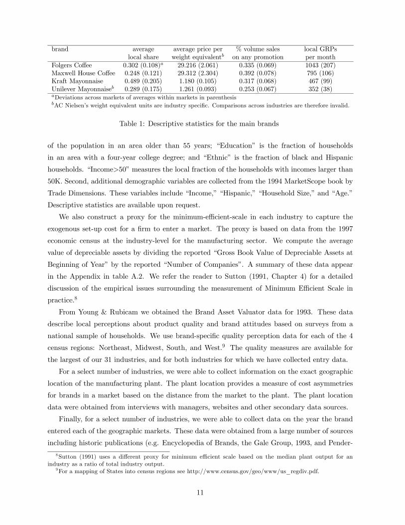
brand average average price per % volume sales local GRPslocal share weight equivalentb on any promotion per month
Folgers Coffee 0.302 (0.108)a 29.216 (2.061) 0.335 (0.069) 1043 (207)Maxwell House Coffee 0.248 (0.121) 29.312 (2.304) 0.392 (0.078) 795 (106)Kraft Mayonnaise 0.489 (0.205) 1.180 (0.105) 0.317 (0.068) 467 (99)Unilever Mayonnaiseb 0.289 (0.175) 1.261 (0.093) 0.253 (0.067) 352 (38)aDeviations across markets of averages within markets in parenthesisbAC Nielsen’s weight equivalent units are industry specific. Comparisons across industries are therefore invalid.
Table 1: Descriptive statistics for the main brands
of the population in an area older than 55 years; “Education” is the fraction of households
in an area with a four-year college degree; and “Ethnic” is the fraction of black and Hispanic
households. “Income>50” measures the local fraction of the households with incomes larger than
50K. Second, additional demographic variables are collected from the 1994 MarketScope book by
Trade Dimensions. These variables include “Income,” “Hispanic,” “Household Size,” and “Age.”
Descriptive statistics are available upon request.
We also construct a proxy for the minimum-efficient-scale in each industry to capture the
exogenous set-up cost for a firm to enter a market. The proxy is based on data from the 1997
economic census at the industry-level for the manufacturing sector. We compute the average
value of depreciable assets by dividing the reported “Gross Book Value of Depreciable Assets at
Beginning of Year” by the reported “Number of Companies”. A summary of these data appear
in the Appendix in table A.2. We refer the reader to Sutton (1991, Chapter 4) for a detailed
discussion of the empirical issues surrounding the measurement of Minimum Efficient Scale in
practice.8
From Young & Rubicam we obtained the Brand Asset Valuator data for 1993. These data
describe local perceptions about product quality and brand attitudes based on surveys from a
national sample of households. We use brand-specific quality perception data for each of the 4
census regions: Northeast, Midwest, South, and West.9 The quality measures are available for
the largest of our 31 industries, and for both industries for which we have collected entry data.
For a select number of industries, we were able to collect information on the exact geographic
location of the manufacturing plant. The plant location provides a measure of cost asymmetries
for brands in a market based on the distance from the market to the plant. The plant location
data were obtained from interviews with managers, websites and other secondary data sources.
Finally, for a select number of industries, we were able to collect data on the year the brand
entered each of the geographic markets. These data were obtained from a large number of sources
including historic publications (e.g. Encyclopedia of Brands, the Gale Group, 1993, and Pender-
8Sutton (1991) uses a different proxy for minimum efficient scale based on the median plant output for anindustry as a ratio of total industry output.
9For a mapping of States into census regions see http://www.census.gov/geo/www/us_regdiv.pdf.
11

gast 1999), the trade press, the manufacturers themselves and the Internet, mainly at manufac-
turer websites. In addition, we consulted the “Hills Brothers” archives at the National Museum
of American History, Washington D.C., which contain marketing and sales records from the 19th
and early 20th centuries.10
4 Documenting the patterns of interest
We now provide a general description of the market structures observed across the 50 geographic
markets and 31 industries. The description of the rawmarket share data generates three distinctive
patterns, which are described in detail for the coffee and mayonnaise industries as examples. To
generlize these findings, we also report summaries of results across the entire set of 31 industries.
First, most of the variation in a brand’s market shares lies in the cross-section of geographic
markets as opposed to the time-series of months.11 Second, the identity of the highest-share
firm in an industry varies across markets, leading to variation in the rank-order of shares across
markets and leading to share asymmetries both within and across markets. Finally, we observe
very strong “spatial dependence” across markets in a brand’s within-market mean share, but not
in deviations from its within-market mean share.
4.1 Decomposition of variance in brand shares
We begin by analyzing the sources of variation in market shares. For many of the industries, the
leading products are physically quite similar. For example, in the ground coffee industry, the
two leading brands, Folgers and Maxwell House differ primarily in less tangible aspects related
to branding. In the absence of product differentiation, one might anticipate aggressive price
competition to eliminate any asymmetries in brand shares within and across markets.
We begin by estimating the within-industry proportion of market share variation for the two
largest (at the national level) brands in the brand/market/time data that is explained by brand
versus market fixed effects. A summary of the R2 levels from each of these 31 regressions (one
per industry) apprears in Table 2. Despite the physical similarities in products within several of
these industries, a strong brand effect emerges across the 2 largest brands in all 31 industries. On
average across industries, brands account for 33% of the total share variation. The full set of 31
industry-specific results are also reported in the first three columns of Table A.3. To simplify the
presentation, results are only reported for a subset of the industries. In the coffee industry, the
10For the mayonnaise industry, entry data were frequently available only at a regional level. In these instances, anexact entry date would need to be inferred, for example by interpolation based on geographically “close” markets.For this reason, our entry analysis will focus on whether a firm had “at least a five year entry advantage” insteadof using the exact entry date of a brand.11Later we will show that this market effect also explains considerably more of the total share variation than
specific retailer effects.
12

N = 62 Brand Market Brand+ Brand×Market Market
min 1% 0% 14% 61%max 53% 97% 98% 99%
median 21% 25% 55% 96%mean 23% 33% 56% 92%
Table 2: Summary statistics for R2 of brand and market fixed effects by brand and industry forthe 2 top selling brands in each of 31 industries.
N=62 Market Timemin 0.505 1.000E-04max 0.998 0.267
median 0.910 0.019mean 0.874 0.040
Table 3: Summary statistics for R2 of market and time fixed effects by brand and industry forthe 2 top selling brands in each of 31 industries.
brand component captures 19% of the share variation. Interestingly, including separate brand and
market effects explains almost half as much share variation as including brand/market interaction
effects, 56% versus 92% respectively on average across industries. These results suggest that,
within an industry, not only is there heterogeneity across brand shares but there is considerable
heterogeneity in a given brand’s share across markets.
The next two columns of Table A.3 build on these findings by reporting a separate decom-
position of the shares for the top two brands in the same subset of industries by markets and
months. A summary of the R2 levels across each of the top two brands and 31 industries appears
in Table 3. For a brand brand, cross-market variation emerges overwhelmingly as the dominant
component of market share variation. On average, markets account for nearly 90% of the share
variation whereas time accounts for roughly 4%. We conclude that the cross-section of markets
captures the majority of the variation in a brand’s share.12
To illustrate the relative importance of cross-market variation versus time-series variation for
brand shares, we use two specific examples. For the top two brands in each of the ground coffee
and mayonnaise data, we plot each brand’s time series for three distinct markets, Kansas City, San
Francisco and Pittsburgh, each from a different region of the US. Each of the plots reveals that the
variation in a brand’s share across these three markets is considerably larger than the variation
12There are several reason for which one might be cautious in interpreting the dominance of the cross-sectionalvariation. First, our data is time aggregated to months, which suppresses the temporal variation. For four of ourindustries, we have analogous sampled at a weekly frequency. In those industries, we observe a similar dominanceof cross-sectional variation. A second potential concern is that our time series may appear to be short. In fact, 3years is considerable longer than typical scanner data bases used in practice, using only a singly market (e.g., onecity or one retail chain).
13

5 10 15 20 25 30 350
0.1
0.2
0.3
0.4
0.5
0.6
0.7
0.8
0.9
1
time
shar
e
Folgers Coffee
Kansas City
Pittsburgh
San Francisco
5 10 15 20 25 30 350
0.1
0.2
0.3
0.4
0.5
0.6
0.7
0.8
0.9
1
time
shar
e
Maxwell House Coffee
Kansas City
Pittsburgh
San Francisco
5 10 15 20 25 30 350
0.1
0.2
0.3
0.4
0.5
0.6
0.7
0.8
0.9
1
time
shar
e
Kraft Mayonnaise
Kansas City
Pittsburgh
San Francisco
5 10 15 20 25 30 350
0.1
0.2
0.3
0.4
0.5
0.6
0.7
0.8
0.9
1
time
shar
e
Unilever Mayonnaise
Kansas City
Pittsburgh
San Francisco
Figure 1: Local time-series variation in shares by brand and several local markets.
across time within each market. In fact, the data appear relatively stationary over time.13 Using
the Dickey-Fuller unit root test (e.g., Hamilton 1994) for Folgers and Maxwell House, we reject
a unit root for 91 of the 100 local time series (i.e. 50 markets and 2 brands). In the mayonnaise
industry, unit roots can be rejected 100% of the time (i.e. for each brand in all 50 markets).
4.2 The geographic dispersion in brand shares
We now examine the distribution of brand shares across markets. First, we look at the coffee and
mayonnaise industries. Figure 2 maps the geographic distribution of within-market mean shares
for the top two ground coffee and mayonnaise brands across our 50 US markets. Each circle’s
radius is proportional to the size of the share in a given market. The maps indicate that brand
shares vary considerably across markets. The average market share of Folgers ranges from 0.15
in Pittsburg to 0.57 in Kansas City. For Maxwell House, average local market shares are between
0.04 (Seattle) and 0.45 (Cleveland). The maps also indicate that, within an industry, the rank-
order of shares varies considerably across geographic areas. Maxwell House shares are strongest
in the northeast, precisely where Folgers is weakest. In general, Folgers clearly dominates the
ground coffee industry in the west and north central markets. But, Maxwell House dominates
the East Coast. Finally, the distribution of shares across markets is clearly not random as we see
strong similarities in brand shares in geographically “close” regions.
13A similar observation regarding share stationarity over time has been suggested by Dekimpe and Hanssens(1995).
14

Folgers Coffee
min:0.15 max:0.57
Maxwell House Coffee
min:0.04 max:0.45
Kraft Mayonnaise
min:0.14 max:0.77
Unilever Mayonnaise
min:0.09 max:0.73
Figure 2: The geographic distribution of share levels across US markets. Circles’ radii are pro-portional to share levels.
The lower half of Figure 2 illustrates similar patterns in the for the two leading mayonnaise
brands, Kraft and Unilever. Geographically, shares are even more dispersed than in the coffee
data. Local shares for Kraft are between 0.14 in New York and 0.77 in Kansas City. For Unilever,
local shares are between 0.09 and 0.73. Spatial patterns also appear in the data insofar as Unilever
shares dominate markets in the North East and West Coast, whereas Kraft shares dominate in
the central and midwestern markets.
Generalizing across the 31 industries, we observe a fair amount of dispersion in a brand’s
shares across markets. Using the top two brands per industry, we see an average dispersion of
0.73 (its standard deviation divided by its mean). In general, this dispersion in brand shares leads
to considerable variation in the rank-orders of shares across markets. Across industries, we see
an average of 8 different brands that are a local share-leader in at least one market, with a range
of 1 to 27. In fact, on average across industries, a local leader dominates a maximum of 64% of
the markets. In only three industries do we observe a single share-leader: Cereals, Cream Cheese
and Frozen Toppings. In both the coffee and mayonnaise industries, we observe four different
local leading brands. For coffee, none of the four brands dominates in more than 52% of the
markets. In mayonnaise, none of the four brands dominates in more than 72% of the markets.
Interestingly, while the largest brands tend to have entered all 50 markets, the average brand in
our database has entered only 11.4 markets, on average. Clearly, the local market structure is
considerably different from the national market structure for most of these industries.
15

4.3 Spatial dependence in brand shares
In addition to geographic dispersion in market shares, Figure 2 also illustrates that a brand’s
shares are spatially dependent i.e., a given brand’s shares co-vary positively acros markets. We
now provide a more formal description of this spatial dependence in brand shares (see Bronnenberg
and Mahajan 2001 and Bronnenberg and Sismeiro 2002 for previous work that has also looked at
spatial covariance in market shares using parametric models).
We use the non-parametric approach of Conley and Topa (2002) to estimate the spatial au-
tocorrelation in brand shares as a function of the distance between a pair of markets. Suppose
the observed share data, ym, are indexed by locations m with coordinates ωm in a Euclidean
space. We assume the dependence between the observations is a function of the physical distance
between their locations. Thus, two random variables, ym and ym0 , become increasingly dependent
as the distance between m and m0 shrinks (i.e. as they become “close”).14 We define the spatial
autocovariance function as:
cov (ym, ym0) = f (Dmm0) (2)
where Dmm0 = kωm − ωm0k is the Euclidean distance between locations m and m0. The spatial
autocovariance function, 2, can be estimated non-parametrically using kernel-smoothing over a
grid of distances. At a given gridpoint δ, the estimated spatial autocovariance is:
bfy (δ) = Xm,m0 6=m
WN kδ −Dmm0k (ym − y) (ym0 − y) , (3)
whereWN kδ −Dmm0k are weights.15 To obtain the corresponding spatial autocorrelation function(ACF), we standardize 5 by the sample variance of y:
bρy (δ) = bfy (δ)var (y)
. (6)
14Formally, we assume our data, ym, are second order stationary and isotropic (i.e. dependent on distance betweentwo locations and not on direction). See Conley (1999) for a more detailed discussion of the regularity conditionsof this model.15We use the uniform kernel with bandwidth η = 200 miles
WN kδ −Dmm0k =
⎧⎪⎨⎪⎩1
Nδif kδ −Dmm0k < η
0 else
, (4)
where Nδ is the number of location pairs within δ±η distance. Defining the distance class Dδη as the combinationsof (m,m0) , m > m0 (because of symmetry), for which kδ −Dmm0k < η, the empirical estimator for the covariancefunction used in this paper reduces to (Cressie 1993):
bfy (δ) = X∀(m,m0)∈Dδη
(ym − y) (ym0 − y)
Nδ. (5)
Experimentation with other kernels (e.g. Gaussian and Bartlett) had little impact on our estimates of the spatialACF.
16

0 500 1000 1500 2000 2500 30000
20
40
60
80
100
120
140
160
180
200
miles
frequ
ency
N = 50 markets
(1275 distance pairs)
Figure 3: Distribution of inter-market distances in miles.
Note that the summation in 3 does not include pairs of observations from the same market
(i.e. where Dmm = 0). Decomposing observed shares into two orthogonal components, an i.i.d.
component and a dependent component, then our our estimate of the covariance, bfy, capturesonly the latter. Then, by construction, the estimated ACF at zero, bρy (0), captures the fractionof total variance in y that is accounted for by the dependent component16.
We test the statistical significance of our ACF point estimates using the bootstrap procedure of
Conley and Topa (2002). The data are re-sampled with replacement from their empirical marginal
distributions to create pseudo-samples that are spatially independent. An acceptance region for
the null hypothesis of spatial independence is constructed using quantiles of the pseudo-sample
estimates of bρ (ym, y0m).The empirical distribution of inter-market distances in the data is reported in Figure 3. Given
the amount of information in the range of distances between zero and 1000 miles, we estimate
the spatial ACF along a grid between 0 and 1000 miles. Figure 4 plots the spatial ACFs for
the within-market mean shares in the ground coffee and mayonnaise industries. That is, the
ACF is estimated for yim = 1T
Pt yimt, where yimt is the market share of brand i in market m
during month t. The 95% acceptance region for the null hypothesis of spatial independence is
also reported. The spatial ACFs are strikingly similar across each of the brands. In each case, the
spatial autocorrelation is positive and significant over a distance of 500-600 miles. A high share
16More formally, suppose that shares can be decomposed into an indiosyncratic as well as a dependent component:
ym = εm + νm
where E (νmνn) = f (Dmn) , E (εmεn) =
½σ2, if m=n0, else
and E (εmνn) = 0. By construction, the estimated ACF
at zero is just bρy (y) = bfy(0)dfy(0)+σ2where the denominator is simply the total geographic sample variance in shares.
17

0 200 400 600 800 1000-0.5
0
0.5
1Folgers Coffee
distance (miles)0 200 400 600 800 1000
-0.5
0
0.5
1Maxwell House Coffee
distance (miles)
0 200 400 600 800 1000-0.5
0
0.5
1Kraft Mayonnaise
distance (miles)0 200 400 600 800 1000
-0.5
0
0.5
1Unilever Mayonnaise
distance (miles)
ACF of sharesACF of sharesACF of shares Bootstrapped Independence RegionBootstrapped Independence RegionBootstrapped Independence Region
Figure 4: Spatial autocorrelation functions (ACF) for within-market mean shares by brand.
in one market coincides with a high share in geographically close markets. Since this dependence
arises from the within-market mean shares, we roughly interpret this pattern as a persistent
“long-run” phenomenon. Finally, the estimate of ACF at zero, bρ (0), roughly corresponds to theproportion of total cross-market variance in share associated with the spatially-dependent error
component. Since bρ (0) exceeds 0.5, we conclude that the co-variation in shares across marketsaccount for a substantial portion of the total cross-market variation in shares.
Next, we estimate the spatial ACF for the within-market deviations from the mean share,
εimt = yimt − yim, for brands i, market m and months t. For each month, we then estimate the
spatial ACF for geographic cross-section of de-meaned shares, εimt. Rather than plot the ACF
for each brand and month, we instead plot the time-averaged ACF as well as the time-averaged
spatial independence region in Figure 5. Our findings fail to reject the null hypothesis of spatial
independence in the monthly deviations from the mean market shares for a brand.17. Further-
more, looking at the estimated correlation at zero distance, bρ (0), we observe that the variance indeviations from the mean share level within a market account for a very small component of the
overall variance in shares across markets. The findings suggest that spatial dependence does not
arise from correlated temporal shocks to shares across markets.
17One can also consider a two-dimensional ACF that considers dependence over time and space. Graphically, wecan plot ACF as a surface over the time and geographic distance dimensions. Our findings revealed no patterns ofinterest in the time-dimension. Hence, we only report dependence patterns in the geographic dimension.
18

0 200 400 600 800 1000-0.5
0
0.5
1Folgers Coffee
distance (miles)0 200 400 600 800 1000
-0.5
0
0.5
1Maxwell House Coffee
distance (miles)
0 200 400 600 800 1000-0.5
0
0.5
1Kraft Mayonnaise
distance (miles)0 200 400 600 800 1000
-0.5
0
0.5
1Unilever Mayonnaise
distance (miles)
ACF of share shocks Bootstrapped Independence Region
Figure 5: Spatial autocorrelation function (ACF) for the temporal shocks in the share data
Correlation at zero distance Correlation between zero and 600 milestop brand second brand top brand second brand
mean 0.59 0.61 0.20 0.20median 0.58 0.53 0.20 0.23min 0.22 0.28 0.01 -0.04max 1.01 1.32 0.46 0.50
Table 4: Summary of Estimated Spatial Correlation Across Industries
The results above pertain only to the coffee and mayonnaise industries. As before, to indicate
generality, we report spatial dependence findings for the within-market mean shares of the top
two brands in each of the 31 industries in the final two colums of Table A.3, in the Appendix.
The table reports the estimated spatial correlation at zero distance, bρ (0), and the average spatialcorrelation over the set of grid points between zero and 600 miles. A summary of these findings
appears in Table 4. On average, the spatially-dependent component of market shares accounts for
over half the total variance. We conclude that understanding the sources of the spatial covariance
are important for understanding the geographic distribution of shares. Similarly, we find that the
spatial correlation is, on average, about 0.2 for cities up to 600 miles apart. Given the distribution
of distances reported in Table 3, this finding suggests that the dependence persists for a large
proportion of our geographic markets.
19

4.4 Sunk costs in CPG industries
In this section we discuss the sources of sunk costs in CPG industries and we motivate the
distinction between endogenous and exogenous sunk costs. We also provide some details about
two industries to highlight the relevance of the theory: coffee and mayonnaise, for which we were
able to collect entry data. We indicate that (1) historically, the dominant brands in each category
originated as regional brands; (2) advertising during local launch of these brands was very intense
and costly; and (3) local leadership tends persist in absence of major innovations.
Firms in CPG industries incur “start up” costs when launching new brands. Such costs
are often sunk and cannot be reversed. The magnitude of some of these costs is given by the
institutions of an industry rather than being determined strategically by a decision maker. An
example of such exogenous fixed costs is the minimum efficient scale of a production facility or
plant. Central to this study, however, other launch costs are endogenous. Firms must invest
in marketing to “position” their brand and to communicate its quality to potential consumers.
Insofar as firms strategically determine the outlays devoted to brand advertising and the image
they wish to create, the magnitude of these costs is endogenous. Furthermore, advertising costs
are considered to be fixed as they do not vary with the quantity sold but rather with the costs
of developing ad copy and the quantity of media time needed. Advertising investments are also
sunk in the sense that quality perceptions resulting from the advertising expenditures can not be
transferred from one brand to the next.
We now briefly discuss the histories of the two categories for which we obtain historic entry
data.
The coffee industry The branded ground coffee industry has a long history in the United
States (see e.g., Pendergast 1999). All of the current large national coffee brands originated as
local brands in different geographic areas between 1848 and 1900. During this early period, firms
relied heavily on advertising to build local market share.18
Folgers, currently the largest national brand, launched in San Francisco in 1848 and expanded
from its San Francisco base eastward. It opened a plant in Kansas City in 1905. Folgers arrived
in Chicago by 1959 (30 years after Hills Bros and Maxwell House). There it could not secure a
better position than the 3rd spot in the market after Hills Bros and Maxwell House, suggesting
that the quality reputation of the two latter firms had become hard to encroach upon. Upon
acquisition by Proctor and Gamble, Folgers became subject to a consent decree by the Federal
Trade Commission to halt further expansion until 1971. Folgers therefore only became truly
national in 1978, when it entered the New England markets.
The second largest national brand, Maxwell House, was launched in Nashville around 1892.
18The ubiquity of advertising is evidenced by a news-paper article at the time that noted that unadvertisedproducts were “the genesis of unsuccessful merchandising” (Pendergast 1999).
20

Maxwell House first entered the markets in the Southern and South-Atlantic states. Next, in 1921
they entered the New England markets, followed by the West and Mid-West markets in 1924 and
1927 respectively. It was the first coffee brand to have national distribution and relied heavily on
advertising during local introduction of their brand (the Gale Group, 1999).
Hills Bros is the third largest national coffee brand. It is was launched in 1881 from San
Francisco and expanded eastward in the 1920’s. It was the first firm to pioneer the use of vacuum
packed cans in 1900, an innovation that the rest of the industry was slow to follow. By 1926,
Hills Brothers was spending a quarter of a million dollars on advertising (most of it in Western
states). It entered the Chicago market in 1930 with an unusually intense marketing including
heavy advertising and mailing all Chicago telephone subscribers a half-pound can of vacuum
packed Hills Brothers Coffee (Pendergast 1999).19
Subsequent innovations in the category, such as the “keyless can” were far less impactful. The
vacuum packed can represents the most substantial innovation in the industry during the 20th
century. It was adopted by most large competitors by the 1920s and 1930s and remains in use as
a standard today.
The mayonnaise industry The mayonnaise industry has traditionally been dominated by
few manufacturers. Hellmann’s introduced mayonnaise to a mass market on the East Coast in
1912, while Best Foods took the West Coast. Both firms subsequently expanded their trade
territories land inward. Best Foods acquired Hellmann’s in 1932, but the Hellmann’s brand name
was maintained in its trade territories. Best Foods was subsequently acquired by Unilever who
nowadays informs its customers that “Best Foods is known as Hellmann’s east of the Rockies.”20
Kraft foods is also a substantial participant in the mayonnaise category with such brands
as Kraft Real Mayonnaise and Kraft Miracle Whip. Miracle Whip was a major innovation for
Kraft in 1933 after it realized that sales of its mayonnaise were slipping and that it needed
a lower priced alternative to mayonnaise in the Depression years. During the introduction of
Miracle Whip, Kraft “launched one of the biggest food advertising campaigns [...] and this
initial effort led to 22 weeks of almost non-stop advertising, including a weekly two hour radio
show.”(http:\\www.kraftcanada.com). Thus, as with the coffee brands, advertising investment ishigh during launch. Despite its late arrival on the market, we hypothesize that Miracle Whip was
effectively a substantial innovation for a sizeable segment of consumers. That is, Kraft was able
to make Miracle Whip a “new entrant” to consumers because to some it provided a new and to
others a better product.
Two smaller manufacturers also have a long history in this category. First, Duke’s Mayonnaise
19The Chicago market up until that time had been a fragmented market with approximately 50 local brands ofwhich only three had more than 25% city-wide distribution (Wilson, 1965).20See for instance http:\\www.mayo.com or http:\\www.hellmanns.com. Hellmann’s and Best Foods have the
exact same ingredients and in the same quantity order.
21

was a first mover in South Carolina and was acquired by C.F. Sauer in 1929. The latter still sells
the Duke’s brand in the Carolina markets. Finally, Blue Plate Mayonnaise is the first major
mayonnaise brand in the New Orleans market in 1927, and it still leads in this market.
After the introduction of Miracle Whip, new product innovation in the category has not been
very frequent and has met with limited success. The most successful innovations in the category
were the introduction of light and cholesterol free mayonnaise in the mid eighties by the incumbent
manufacturers. Regular mayonnaise, which remains the bulk of category volume, has remained
largely unchanged in appearance and taste since the popularization of the aforementioned brands
in the twenties and thirties.
Discussion Historically, most large national CPG brands evolved from regional brands. These
regional brands used advertising as a means to enhance their quality image in existing markets.
All large national brands today initially launched with large-scale local advertising campaigns.
Interestingly, while major shifts in local market shares do not occur in the coffee and mayonnaise
categories, there are cases where later entrants (e.g., Folgers in New England) try hard to break
into new markets. In such cases, the early entrants generally sustain a strong market share
advantage. This suggests that the strategic first mover advantage, which initially is based on
pre-emption through advertising investments later is also supported by accumulated advertising
investments.
The current market structures (assortment of brands and relative shares) in both the coffee
and mayonnaise industries have been in place for a long time. Neither of these categories has
seen major successful innovations in the last decennia. An interesting issue is how one defines
initial conditions in an industry. The theory we present looks at the product entry date. However,
one might consider whether initial conditions can be re-formulated during periods of important
product innovation. That is, one might consider comparing the date of product launch versus the
date of launch of a radical innovation as two alternative definitions of “entry.”
5 Testing the predictions of ESC theory
In this section, we establish an empirical link between these empirical patterns and the ESC
framework mainly by looking at several moments of the empirical distribution of market shares.
We proceed in several steps. First, we test the basic predictions of the theory relating concen-
tration levels and market size. Second, we test for a first-mover effect in observed market share
levels as well as share co-movements across markets. Third, we attempt to rule out alternative
explanations for the main patterns in our data. Finally, we discuss the results in the context of
the emergence and sustainability of local oligopolies in CPG markets.
22

5.1 Concentration and market size
Our first objective is to establish that advertising introduces an element of vertical differentiation
by testing for a lower bound in concentration in larger markets for advertising-intense industries,
as opposed to non-advertising-intensive industries. The theory predicts a lower bound in the
case of ESC because of a competitive escalation in advertising in larger markets amongst a finite
number of firms.
We define the advertising-intensity of an industry by looking at the total advertising investment
during and before the sample, 1989 to 1995, scaled by total in-sample industry revenues, 1993
to 1995. The upper and lower quartiles of industry advertising-intensity designate the sets of
advertising-intense versus non-advertising-intense industries21. We measure concentration using
the share of the largest-share brand, C1, in each industry and geographic market.22 We also
consider two measures of market size based on the natural logarithm of the total revenues for an
industry within a market as well as the natural logarithm of the population of a geographic market.
The revenue and population data are first normalized by an industry’s minimum efficient scale
(MES as defined in the data section) to control for the exogenous fixed set-up costs associated with
entering into a given industry.23 In the case of population, the use of a dollar-value normalization
is not as intuitive, but we retain this measure to demonstrate robustness of our results.
The escalation in advertising for larger markets is clear in Figure 6, which plots average
industry advertising expenditure per brand, by market, between 1993 and 1995 against market
size measured as the logarithm of revenues over MES. The figure drops the bottom quartile of
industries based on advertising-intensity as advertising expenditures tend to remain either zero or
close to zero across markets in these industries. A regression of the logarithm of average industry
advertising in a market on the logarithm of market size and industry fixed-effects generates a
statistically significant market-size elasticity of advertising of roughly one. We plot the predicted
advertising levels in the figure to visualize this escalation.
We now test whether this advertising escalation leads to a lower bound in concentration, as
predicted by the theory. In Figure 7, we provide a scatterplot of observed concentration levels
and market size across industries and geographic areas in our raw data. We provide plots for
both advertising-intensive and non-advertising-intensive industries. For the advertising-intensive
industries, there is little evidence of a linear correlation between concentration and market size.
Furthermore, even in the largest markets, concentration seldom falls below 20%. Although not
21This may not an ideal measure of advertising intensity as it is based on equilibrium outcomes of advertisingand sales. A preferable approach would be to use some measure of the marginal effectiveness of advertising in anindustry. But, such measures are not readily available.22Our substantive results comparing advertising-intensive to non-advertising-intensive results are comparable if
we consider a 2,3 or 4-firm concentration ratio.23The results in this section are qualitatively similar if we disregard the minimum efficient scale measures and
proceed as if ESC are the only relevant fixed costs and we relate concentration to the logarithm of revenues.
23

-4 -3 -2 -1 0 1 2 3 4 50
0.1
0.2
0.3
0.4
0.5
0.6
0.7
0.8
0.9
1
mea
n ad
verti
sing
($10
0,00
0)
log (revenues/MES)
Figure 6: Advertising expenditure per month versus market size excluding the bottom quartileindustries based on advertising intensity. The solid line corresponds to the predicted advertisinglevels from a regression of log-advertising on industry fixed-effects and market size.
reported, a regression of concentration on market size reveals a statistically significant concave
relationship under both market size definitions.24 In contrast, there is less evidence of a bound
in non-advertising-intensive industries where we observe concentration levels as low as 5%. A
regression of concentration on market size reveals a downward-sloping linear relationship in the
case of non-advertising-intensive industries.
To test the theory, we need to formalize our analysis of the lower bound. We use the same
approach as the extant literature (e.g. Sutton 1991 and Robinson and Chiang 1996) by estimating
a lower bound function using the statistical approach of Smith (1994). One can think of the
share of the largest firm, C1 as an extreme value of the distribution of brand shares. Since
we are interested in testing for a bound, we assume C1 is drawn from a Weibull distribution,
which is bounded below. Formally, we assume concentration in market m has the following form:
C1m = B (market sizem)+ωm, whereB (market sizem) is a parametric function of observed market
size that characterizes the lower bound. The random variable ωm is distributed according to the
Weibull distribution with shape parameter α and scale parameter β. Since C1 is constrained to lie
between zero and one, we instead use a logit transformation, eC1m ≡ log³ C1m1−C1m
´. Finally, since
we expect concentration to be inversely-related to market size in smaller markets, we follow the
24Sutton (1991) also finds similar evidence of a non-monotonic relationship between concentration and marketsize for advertising-intensive industries. This non-monotonicity is consistent with the theory.
24

0 2 4 6 80
0.2
0.4
0.6
0.8
1
log (revenues/MES)
1-fir
m c
once
ntra
tion
Advertising-Intensive Industries
0 2 4 6 80
0.2
0.4
0.6
0.8
1
log (revenues/MES)
1-fir
m c
once
ntra
tion
Non-Advertising-Intensive Industries
4 6 8 100
0.2
0.4
0.6
0.8
1
log (population/MES)
1-fir
m c
once
ntra
tion
Advertising-Intensive Industries
4 6 8 100
0.2
0.4
0.6
0.8
1
log (population/MES)
1-fir
m c
once
ntra
tion
Non-Advertising-Intensive Industries
Figure 7: Concentration versus Market Size in relatively advertising-intensive and non-advertising-intensive industries.
literature and specify B (market sizem) as a quadratic polynomial in the inverse of market size:
eC1m = a+b
market sizem+
c
(market sizem)2 + ωm. (7)
This parametric formulation also provides us with a characterization of the limiting concentration
as the market size approaches infinite: a = log³
C1∞1−C1∞
´when market size approaches infinite.
We estimate the parameters for the bound function, (a, b, c)0, and the Weibull distribution,
(α, β)0, using the two-step procedure suggested by Smith (1994).25 Standard errors are computed
using the simulation method discussed in Smith (1994).
Estimation results are reported in Table 5. In general, we observe a steeper bound function for
non-advertising-intensive industries, driven mainly by the linear as opposed to the quadratic term.
To illustrate, we plot the estimated bound functions in Figure 8, using revenues as market size,
and in Figure 9, using population as market size. Furthermore, the estimated limiting bounds
reported in Table 5, C1∞, are much lower for non-advertising-intensive than for advertising-
intensive industries (about 15% and less than 5% respectively). The estimated limiting bounds
are not statistically different from zero at the 95% confidence level in the case of non-advertising-
25 In the first stage, we estimate (a, b, c)0 from (7) using a simplex search subject to the constraint eC1m − a −b
market sizem− c
(market sizem)2≥ 0. In the second stage, parameters (α, β)0 are estimated by fitting the first-stage
prediction errors to a Weibull distribution.
25

Concentration versus Concentration versusrevenues/MES population/MES
Ad-Intensive Non-Ad-Intensive Ad-Intensive Non-Ad-Intensivecoefficient s.e. coefficient s.e. coefficient s.e. coefficient s.e.
a -1.74 0.07 -3.07 0.22 -1.90 0.21 -7.48 1.15b 0.63 0.22 2.22 0.71 1.56 1.48 39.02 10.92c -0.02 0.04 0.00 0.19 4.77 1.54 0.01 29.26α 1.18 0.03 1.90 0.05 1.19 0.04 2.10 0.05β 1.97 0.07 2.34 0.09 1.91 0.08 2.36 0.10
C1∞ 0.15 0.01 0.044 0.023 0.13 0.05 0.01 0.01log-likelihood 271.18 395.45 279.97 429.86
Table 5: Estimated Lower Bound Functions for concentration in advertising-intensive and non-advertising-intensive industries.
0 2 4 6 80
0.2
0.4
0.6
0.8
1
log (revenues/MES)
1-fir
m c
once
ntra
tion
Advertising-Intensive industries
0 2 4 6 80
0.2
0.4
0.6
0.8
1
log (revenues/MES)
1-fir
m c
once
ntra
tion
Non-Advertising-Intensive industries
Figure 8: Estimated lower bounds on concentration for ad-intensive versus non-ad-intensive in-dustries (using log revenues)
intensive industries. These results are all consistent with the theory. Our findings suggest that
concentration is bounded away from zero in advertising-intensive industries, but not in non-
advertising-intensive industries.
5.2 Brand proliferation
The concentration results documented above relate directly to the observed escalation in industry
advertising in larger markets. The theory generates a related prediction placing an upper bound
on the number of advertised brands as market size grows. However, we may nevertheless observe
a proliferation in the total number of brands if the market can sustain non-advertised “fringe”
brands, which will increase in number as market size grows. Ellickson (2004) documents evidence
of a similar two-tiered market structure with dominant and fringe firms in the context of super-
26

4 6 8 100
0.2
0.4
0.6
0.8
1
log (population/MES)
1-fir
m c
once
ntra
tion
Advertising-Intensive industries
4 6 8 100
0.2
0.4
0.6
0.8
1
log (population/MES)
1-fir
m c
once
ntra
tion
Non-Advertising-Intensive industries
Figure 9: Estimated lower bounds on concentration for ad-intensive versus non-ad-intensive in-dustries (using log population)
markets. He finds that the number of high quality supermarkets remains fixed across markets of
varying size, whereas the number of low-quality supermarkets increases in larger markets.
In our data, we observe a co-existence across markets and industries of brands that advertise
and brands that do not. In table A.4, in the Appendix, we report the average (across markets
and time) number of brands and market share levels for advertised versus non-advertised brands
in each of the industries. For these results, we drop the private labels to focus on the proliferation
of small local brands; although adding private labels would merely strengthen our results below.
We summarize these findings in table 6. We use the historic advertising as a proxy for investment
in the sunk cost. Hence, our classification of advertising versus non-advertising brands is based
on whether a brand invested in advertising (i.e. the sunk cost) during the years 1989-1993.26
The typical market for any given industry has considerably more non-advertised brands than
advertised brands. The number of non-advertised brands can be as large as 19, whereas the
number of advertised brands never exceeds 6, on average. Interestingly, the mean share of an
advertised brand is considerably larger than that of an non-advertised brand, on average. In this
respect, our distinction between the former and the latter seems to be catpuring a distinction
between large brands and a “fringe”.
We next test the proliferation prediction by pooling our 31 industries and 23 geographic
markets for which we observe advertising. Since the the number of brands is a count variable,
26For the results reported, we define an advertising brand as one that advertises during each year in our data. Anon-advertising brand is defined as one that never advertised during the sample years. Although not reported, allof our results are robust to less conservative definitions that consider brands that “occasionally” advertise (i.e. upto less than half the time) and brands that “occasionally” do not advertise (i.e. less than half the time).
27

market share number of brandsmean min max mean min max
Advertising Brands 0.27 0.06 0.68 1.39 0 6.04Non-Advertising Brands 0.07 0.02 0.21 8.14 1.26 19.22
Table 6: Summary of advertising versus non-advertising brands across all 31 industries
Number of Brands versus Number of Brands versuslog(revenues/MES) log(population/MES)
Advertising Non-Advertising Advertising Non-AdvertisingBrands Brands Brands Brands
coefficient s.e. coefficient s.e. coefficient s.e. coefficient s.e.intercept 0.89 0.14 1.58 0.09 0.95 0.13 1.70 0.09
log(market size) 0.07 0.06 0.11 0.02 0.02 0.06 0.10 0.03log-likelihood -615.82 -1577.04 -616.50 -1579.82
Table 7: Brand proliferation and market size. The log(market size) terms are included in devia-tions from their mean level. Each regression also includes industry fixed-effects.
we run a Poisson regression of the number of advertised brands in an industry and geographic
market on industry fixed-effects and market size.27 We then run the same regression using the
number of unadvertised brands as the dependent variable. Results are reported in Table 7, where
market size is approximated as either the natural logarithm of the ratio of population to minimum
efficient scale or as the natural logarithm of the ratio of revenues to minimum efficient scale. As
expected, we find a statistically insignificant relationship between market size and the number of
advertising brands. However, we do find a statistically significant relationship between market
size and the number of fringe brands. These findings are robust to both our definitions of market
size. These results suggest that the number of non-advertising brands increases with market size,
while the number of advertising brands does not.
Finally, we revisit the lower bound on concentration by estimating a separate bound within
the segment of advertised brands and the segment of non-advertised brands. In each case, we
use the maximum share within a segment-industry-market. We also restrict our attention to
the advertising-intensive industries, as defined in the previous section. Parameter estimates are
reported in Table 8 and graphical results are reported in figure 10. As expected, the estimated
bounds function is steeper for the non-advertised brands. In fact, just looking at the raw data
we can see that concentration falls with market size for the segment of non-advertised brands.
27Formally, we assume the number of brands of a given type t (t =advertise or no advertise) in an industry i andmarket m, Nimt, are distributed Poisson with mean λimt where:
λimt = exp (Ximβt)
and Ximt are characteristics of industry i which is of type t in market m.
28

Advertising brands Non-Advertising Brandscoefficient s.e. coefficient s.e.
a -1.73 0.17 -4.80 0.64b 9.9*e-4 0.94 7.57 4.51c 5.7*e-4 1.92 -1.51 7.39α 1.26 0.06 1.39 0.06β 1.99 0.12 2.24 0.15
C1∞ 0.15 0.05 8.2*e-3 0.01log-likelihood 117.33 136.94
Table 8: Estimated bound function for advertised versus non-advertised brands in the advertising-intensive industries.
0 2 4 6 80
0.2
0.4
0.6
0.8
1
log (revenues/MES)
1-fir
m c
once
ntra
tion
Advertising Brands
0 2 4 6 80
0.2
0.4
0.6
0.8
1
log (revenues/mes)
1-fir
m c
once
ntra
tion
Non-Advertising Brands
Figure 10: Estimated lower bounds on concentration in the advertising-intensive industries foradvertised versus non-advertised brands.
Furthermore, the limiting bound appears to be much lower than that of the advertised brands.
In Table 5, we report the limiting lower bounds in each case finding a lower bound of 0.15 for
advertising-intensive industries and 0.0082 for non-advertising-intensive industries. These results
confirm that in advertising-intensive industries, the set of non-advertised brands fragments while
the set of advertised brands does not. Thus, non-advertised brands develop a sub-market-structure
ressembling the prediction of an exogenous sunk costs market.
5.3 Order of entry effects
We now investigate the impact of historic order-of-entry on the geographic distribution of market
shares. Unfortunately, historic entry data are not readily available for all 31 industries (in contrast
with current share and marketing data) and need to be collected manually. We focus this analysis
on two industries, coffee and mayonnaise, for which we collected entry patterns from various
29

Folgers Coffee
min:0.15 max:0.57
Maxwell House Coffee
min:0.04 max:0.45
Kraft Mayonnaise
min:0.14 max:0.77
Unilever Mayonnaise
min:0.09 max:0.73
Figure 11: The joint geographic distribution of share levels and early entry across US markets.Circles are proportional to share levels. Shaded circles indicate a brand locally moved first.
sources. Whereas our analysis thus far has generalized across 31 industries, focusing on two
industries limits the generalizeability of our results on order-of-entry. Nevertheless, the spatial
patterns explained by order-of-entry are observed across other advertising-intensive industries
and, hence, our analysis in this section can be seen as a preliminary attempt to explain a general
phenomenon.
Figure 11 contains a plot of the US geographic maps for the two leading brands in each of the
ground coffee and mayonnaise industries. To indicate the order-of-entry patterns, we use a shaded
circle for markets where the brand had at least a 5 year entry advantage and an open circle for
markets where it did not. Hence, the maps give a graphical representation of the joint distribution
of a brand’s shares and early entry status across markets. For example, Folgers started in the
West and moved East whereas Maxwell House started in the East and moved West. The maps
also reveal a strong positive correlation between a brand’s share level and its early entry status.
Entry status also appears to exhibit a similar spatial covariance as a brand’s shares.
We now look at the relationship between shares and entry more formally. The main objective
is to test whether early entry status explains the observed share levels across markets. Unlike
Mazzeo and Cohen (2003), we treat historic entry as exogenous28. In the coffee category, we
include a third brand, Hills Brothers, to ensure that we always have the top two brands in each
28Since the brands we study originated during the mid to late 19th century, it is unlikely that technology at thetime would have been adequate to coordinate a national role-out. Similarly, it is unlikely that a firm selected an“optimal” target market to initialize the diffusion of its brand across the US.
30

Coffee Share, N=150Entry, Brand
Entry Brand Entry and and Demo-Effect Effects Brand Effects graphic Effects
Variables coefficient s.e. coefficient s.e. coefficient s.e. coefficient s.e.Intercept 0.135 0.011 0.057 0.014 0.050 0.010 0.355 0.370Folgers 0.245 0.020 0.200 0.015 0.200 0.014
MaxwellHouse 0.191 0.020 0.086 0.017 0.086 0.016Hills BrosFirstEntry 0.202 0.019 0.170 0.015 0.170 0.014
R2 0.440 0.536 0.756 0.776Mayonnaise Share, N=100
Entry, BrandEntry Brand Entry and and Demo-Effect Effects Brand Effects graphic Effects
Variables coefficient s.e. coefficient s.e. coefficient s.e. coefficient s.e.Intercept 0.245 0.019 0.289 0.027 0.187 0.019 0.066 0.797
Kraft 0.200 0.038 0.141 0.025 0.142 0.025Unilever
FirstEntry 0.327 0.028 0.298 0.025 0.293 0.025R2 0.577 0.220 0.681 0.688
Table 9: Impact of entry on share levels
market. In table 9, we report regression results, by industry, for share levels on brand and early
entry status. The dependent variable is the within-market mean share for each brand. We
define “FirstEntry” as an indicator for whether or not a brand had at least a 5 year first entry
advantage in a market. We report results from four models. In the first, we include only entry;
in the second we include only brand effects; in the third we inlclude both brand and entry; and
in the fourth we include demographic variables.29 In both industries, we find that entry alone
explains a non-trivial portion of the total cross-sectional variation in shares, 44% in coffee and
58% in mayonnaise. Conditioning on both entry and brand accounts for 76% of the variation in
coffee and 68% in mayonnaise. In coffee, early entry status appears to generate roughly a 17%
benefit to share level. In mayonnaise, early entry generates a 29% share benefit. The entry effects
are fairly robust both to the inclusion of brand effects and the inclusion of demographic variables.
However, the brand effects are sensitive to the inclusion of entry as, in both industries, the brand
effects fall once entry is accounted for. Finally, the magnitude of the entry effects are such that
the rank-order of shares for the top brands will be influenced by the order of entry.
To check the robustness of our entry effect, we now investigate the impact of entry on perceived
quality levels for these brands. Unlike market share, which is an outcome of the ESC investment,
29The demographic variables control for exogenous market-specific characteristics to reflect local demand condi-tions.
31

Coffee Perceived Quality, N = 150Entry, Brand,
Entry Brand Entry and and Demo-Variables Effect Effects Brand Effects graphic Effects
coefficient s.e. coefficient s.e. coefficient s.e. coefficient s.e.Intercept 0.116 0.003 0.094 0.003 0.093 0.003 0.163 0.104Folgers 0.061 0.005 0.055 0.005 0.055 0.004
Maxwell House 0.041 0.005 0.025 0.005 0.025 0.005Hills BrosFirstEntry 0.036 0.005 0.026 0.005 0.026 0.004
R2 0.229 0.527 0.615 0.706Mayonnaise Perceived Quality,N = 100
Entry, Brand,Variables Entry Brand Entry and and Demo-
Effect Effects Brand Effects graphic Effectscoefficient s.e. coefficient s.e. coefficient s.e. coefficient s.e.
Intercept 0.485 0.004 0.473 0.003 0.465 0.003 0.494 0.134Kraft 0.054 0.005 0.049 0.004 0.049 0.004
UnileverFirstEntry 0.034 0.006 0.024 0.004 0.026 0.004
R2 0.227 0.570 0.680 0.685
Table 10: Impact of Entry on Perceived Quality Levels
the perceived brand quality is a more direct measure of the ESC investment itself. The Y&R
measures of perceived brand quality for each brand and market serve as the dependent variable.
Results appear in table 10. As before, entry explains a substantial portion of the total variation in
perceived brand quality across markets in both coffee and mayonnaise (23% in both industries).
The scale of these measures is really ordinal in nature, so we do not attribute much importance to
the levels of our parameter estimates. Nevertheless, as before, conditioning on entry does slightly
lower the expected quality differentials across brands within a market.
Finally, we show that entry has a similar predictive ability for a brand’s advertising intensity
(in GRPs) across markets. We measure a brand’s advertising intensity in a market as its “share
of voice” (its share of total advertising GRPs for the industry). Results are reported in Table
11, where a separate entry coefficient is estimated for each brand. For most of the brands, we
observe a positive impact of entry on advertising intensity. An exception is Folgers, which has a
significantly negative coefficient. Folgers tends to advertise in markets where the coffee category
is relatively large. In effect, Folgers advertises more strongly in markets where the category
development index (CDI) is high.30 In contrast, Maxwell House, Unilever and Kraft all advertise
more aggressively where their respective brand development indeces (BDI) are high.31 Marketing
30The category development index (CDI) measures the importance of a geographic market to an industry as thatmarket’s share of the national industry revenue, relative to the market’s share of national grocery dollar volume.31The brand development index (BDI) in a market is defined that market’s share a manufacturer’s brand revenue
32

Coffee, N = 69 Mayonnaise, N = 46Entry and Entry and
Brand Effects Brand EffectsVariables Coefficient s.e. Variables Coefficient s.e.Intercept 0.024 0.006 Intercept 0.400 0.014Folgers 0.329 0.009 Kraft 0.104 0.021
Maxwell House 0.255 0.010 UnileverHills Bros Entry Kraft 0.073 0.022
Entry Folgers -0.024 0.011 Entry Unilever 0.074 0.022Entry MH 0.022 0.011Entry HB 0.011 0.019
R2 0.969 R2 0.645
Table 11: Impact of entry on advertising levels
practitioners routinely use CDI and BDI to help allocate marketing resources across geographic
areas (see Kotler 2000, pages 124-25 for a discussion). In the data, the correlation between BDI
(CDI) and advertising share of voice in the coffee industry is 0.33 (0.15) and 0.41 (0.04) for
Folgers and Maxwell House, respectively. In the mayonnaise industry the correlation between
BDI (CDI) and advertising share of voice is 0.86 (0.03) and 0.77 (−0.07) for Kraft and Unilever,respectively. Since entry has a strong impact on shares, it is therefore not surprising to observe a
strong correlation between entry and advertising for BDI-driven firms. In fact, standard practice
of BDI-based advertising decisions is entirely consistent with the equilibrium in our model of ESC
with sequential entry. Although we do not observe entry data for other industries, we do observe
an average correlation between share of voice and BDI (CDI) of 0.36 (−0.03) for the 2 largestbrands and the 31 industries. This finding suggests most firms allocate advertising resources in a
manner that protects their strong markets.
We now examine the impact of entry on the co-variation in shares across markets. We estimate
a spatial autocovariance function for the residuals from the share regression in column four of Table
9 which capture the variation in shares net of entry and market demographics. Standardizing by
the variance of the residuals gives us the spatial auto-correlation of the residuals. As before, the
spatial auto-correlation at zero indicate the proportion of variance in the residuals accounted for
by a spatially-dependent component. A plot of the estimates appears in Figure 12, indicated by
the squares. The dotted lines correspond to the 95% acceptance region for independence. We
also plot the original ACF of the raw shares, indicated by the circles. The results indicate that,
after conditioning on entry, the dependent component of shares becomes very small relative to
the total variance. In both industries, the share of variance accounted for by the dependent
component falls by over 50%. We conclude that entry accounts for a sizeable proportion of the
spatial dependence observed in the data.
relative to that market’s share of the national industry revenue.
33

0 200 400 600 800 1000-0.5
0
0.5
1Folgers Coffee
distance (miles)0 200 400 600 800 1000
-0.5
0
0.5
1Maxwell House Coffee
distance (miles)
0 200 400 600 800 1000-0.5
0
0.5
1Kraft Mayonnaise
distance (miles)0 200 400 600 800 1000
-0.5
0
0.5
1Unilever Mayonnaise
distance (miles)
SpatCov(share)/Var(share) SpatCov(residuals)/Var(share) Bootstrapped independence region
Figure 12: Accounting for spatial covariation using Entry.
The theory predicts that order-of-entry will influence the rank-order of market shares in
advertising-intensive industries. For two of our industries, we find that entry is a very good
predictor for a brand’s share levels, accounting for a large proportion of the total geographic vari-
ance in shares. In fact, the rank-order of shares appears to be directly influenced by entry status,
even after controlling for brand-specific effects. Furthermore, we have shown that entry accounts
for a large proportion of the geographic covariance in a brand’s shares across markets. We find
that the proportion of total share variance accounted for by the dependent component across mar-
kets falls over 50% once entry is accounted for. Thus, the historic geographic diffusion of brands
across geographic markets appears to be a good predictor of the observed spatial dependence in
current market shares. We have also shown that early entrants advertise more aggressively for
firms using BDI advertising allocation rules. These results are consistent with the prediction of
the theory whereby an early entrant advertises more aggressively and, in turn, garners a higher
market share in equilibrium.
5.4 Alternative explanations
In the previous sections, we establish a connection between the the asymmetric share patterns,
for coffee and mayonnaise, and historic entry patterns. In this section, we test several potential
34

sources of firm heterogeneity that could also explain these patterns. First, we consider geographic
cost advantages based on a brand’s proximity to its production plant (Greenhut and Greenhut
1988). Second, we test for relationships with specific multi-market retailers. Manufacturers
frequently pay slotting allowances to retailers to obtain premium shelf space for their products
(Federal Trade Commission 2001, Israilevich 2004, Sudhir et al. 2004). Third, we look for parent
company effects in the case that specific food companies might possess regional advantages that
are passed-on to each of its brands. In addition to firm heterogeneity, we also look at alternative
strategic asymmetries that could explain these patterns. Specifically, we look at the role of prices
and promotions in explaining the cross-market share patterns.
In table 12, we continue the analysis of share levels across markets for coffee and mayonnaise as
we did with entry in table 9. In the first column, we repeat the brand-only effect. In the second
column, we add the distance of each brand to its nearest manufacturing plant. The distance
effect is insignificant in both industries, suggesting that proximity to production facilities does
not engender a strategic advantage in either industry.
In the third and fourth columns, we look at the correlation between shares and the log of prices
and promotions, respectively, after controlling for brands. In both industries, these effect sizes
are very small and, in the case of promotions, insignificant. One must be cautious in interpreting
these effects as there is clearly a simultaneity problem since firms set prices and promotions
in anticipation of their respective impacts on shares. Nevertheless, it is surprising how relatively
uncorrelated prices and promotiones are with the cross-section of shares.32 Although not reported,
we also computed the ratio of the estimated spatial covariance in the residuals of the regression
of shares on prices (and on promotions) to the variance of shares. At a zero distance, we obtain
values of roughly 0.70 for prices and 0.83 for promotions. These results indicate that very little of
the spatial covariance in market shares is accounted for by either of these two marketing variables.
The lack of a promotinal effect is particularly interesting since promotions represent a form of
awareness advertising. Typical promotions include feature ads in newspapers and in-aisle displays
in the retail stores that do not contain any specific product or brand quality information, in
contrast with television advertising. In the final column, we pool all the various effects, including
entry and demographics. Comparing back to the previous section, we can see that the entry
effect is very robust to these other explanations. Overall, we conclude that entry seems to be
a considerably better predictor both of expected share levels and of the spatial covariation in a
brand’s share levels across markets.32 In contrast, price and promotion variables are often strongly related to the within-market temporal differences
in brand shares. We run a separate regression of shares on prices and/or promotions for each of the top two brandsin each industry and each of the 50 markets. That is, we run 100 regressions per indstry (2 brands and 50 markets).On average, the R2 of price is 0.21, for promotion it is 0.27 and for both combined it is 0.37. It is clearly notpossible to interpret causation from such regressions. Our objective here is merely to indicate that prices andpromotions do appear to co-move with shares over time, even though they do not across markets.
35

Coffee Brand Distance Price Promo Allcoeff. s.e. coeff. s.e. coeff. s.e. coeff. s.e. coeff. s.e.
Intercept 0.057 0.014 0.062 0.019 1.247 0.269 0.107 0.034 1.158 0.454Folgers 0.245 0.020 0.246 0.020 0.283 0.020 0.265 0.023 0.255 0.021
Maxwell House 0.191 0.020 0.191 0.020 0.231 0.021 0.202 0.021 0.123 0.021Hills BrosFirstEntry 0.161 0.015
MinDistToMnfr -0.009 0.024 -0.034 0.016log(Price) -0.364 0.082 -0.122 0.074log(Promo) 0.063 0.039 0.108 0.035
R2 0.536 0.536 0.590 0.544 0.796Mayonnaise Brand Distance Price Promo All
coeff. s.e. coeff. s.e. coeff. s.e. coeff. s.e. coeff. s.e.Intercept 0.289 0.027 0.306 0.040 0.438 0.056 0.312 0.112 0.366 0.750
Kraft 0.200 0.038 0.200 0.038 0.157 0.039 0.197 0.042 0.090 0.027Unilever
FirstEntry 0.273 0.024MinDistToMnfr -0.024 0.039 -0.105 0.036
log(Price) -0.652 0.218 -0.576 0.166log(Promo) 0.016 0.077 0.061 0.052
R2 0.220 0.223 0.285 0.220 0.737
Table 12: Impact of various firm asymmetries on share levels
We now consider the potential role of multi-market retailers in influencing the geographic
distribution in brand shares. The practice of slotting-fees could enable a manufacturer to establish
a relationships with specific retail chains, which could in turn generate regional advantages in
distribution. We can test this effect by checking whether brand share variation exhibits a retail
account component in the retail account-level data. A retail account is a combination of a retail
chain and a geographical market. This data cannot separately identify a retailer and a market
effect for retailers operating in a single geographic market. Instead, retail account effects are
tested using dummy variables for retail chains operating in multiple geographic markets (e.g.
Albertsons, Safeway and Krogers). For each of the top two brands in each of the 31 industries,
we pool all the retail accounts, markets and months and decompose the variance. In general, the
R2 from retail account fixed-effects are very small compared to market fixed-effects. For instance,
market fixed-effects and retailer fixed-effects explain 62% and 14% of the variation in market
shares respectively. Similarly, in the mayonnaise industry, market and retailer effects explain
85% and 5% of the share variation respectively. For a few of the smaller industries, retailer
effects are larger due to the fact that not all retailers carry them (e.g. refrigerated pasta) or that
private labels are strong in some chains and not others. Across all industries, the retail component
accounts for 20% of share variation, on average, whereas the market component accounts for more
36

5 10 15 20 25 300
0.1
0.2
0.3
0.4
0.5
0.6
0.7
0.8
0.9
1
time
shar
e
Kraft Mayonnaise
(Albertsons only)
Denver
Los Angeles
5 10 15 20 25 300
0.1
0.2
0.3
0.4
0.5
0.6
0.7
0.8
0.9
1
time
shar
e
Kraft Mayonnaise
(entire market)
Denver
Los Angeles
5 10 15 20 25 300
0.1
0.2
0.3
0.4
0.5
0.6
0.7
0.8
0.9
1
time
shar
e
Unilever Mayonnaise
(Albertsons only)
Denver
Los Angeles
5 10 15 20 25 300
0.1
0.2
0.3
0.4
0.5
0.6
0.7
0.8
0.9
1
time
shar
e
Unilever Mayonnaise
(entire market)
Denver
Los Angeles
Figure 13: Brand shares in the mayonnaise industry with retailers and in markets
than 51%.
To illustrate these findings, we focus on the retailer Albertsons, which has presence in the
West and South regions of the United States. Albertsons’ operations in the Denver and Los
Angeles markets are sourced by the same buying office. Hence, the Albertsons data for these two
markets reflect not only the same retailer, but also the same purchasing agent. In Figure 13,
we plot the time series of the Kraft and Unilever brand shares in the mayonnaise industry, the
two dominant products in the industry. On the left panels, we report the share history of each
brand within Albertsons by market. On the right panels, we report the share history of each
brand for the entire market (i.e. all retailers in the market) by market. In the graph, we can see
that the market-specific component of the share histories is considerably more influential than
the retailer or time components. The within-Albertsons panels correspond very closely to the
market-level results. Also, the week-to-week fluctuations in shares are extremely small relative to
the cross-market fluctuations.
Overall, we conclude that none of these alternative explanations is capable of explaining the
geographic patterns we observe in our brand shares. Furthermore, the entry effect appears to be
robust, even after controlling for these various alternative firm asymmetries.
37

6 Conclusions
We test the implications of a model of endogenous sunk advertising costs using brand data for 31
CPG industries. Consistent with the theory, the results indicate a lower bound on the relationship
between concentration and market size for advertising-intense industries. However, in the case
of non-advertising-intense industries, no such lower bound is established and, in larger markets,
these industries tend to fragment. Consistent with these findings, we also observe an escalation in
the level of advertising in larger markets. We do not, however, observe an escalation in the number
of advertised brands in larger markets. In contrast, we observe a positive relationship between the
number of un-advertised brands and market size, suggesting a proliferation of “fringe” brands in
larger markets. These results are consistent with a theory in which fixed (and sunk) investments
in brand advertising shift out consumer willingness-to-pay. For advertising-intensive industries,
increasing market size leads to an escalation in advertising outlays as opposed to entry, which in
turn leads to non-fragmentation.
For two industries, we also test for a an early-mover effect on current shares. In each of
these industries, we find that entry impacts the levels and rank-orders of market shares for the
top brands in a market. A comparable entry effect emerges for perceived brand quality, which
is also consistent with the theory. In addition, we find that for the most of the brands studied,
we observe a strong first-entry effect on advertising “share of voice.” Our entry effects can only
be established for two industries. However, we find that entry explains almost all of the spatial
dependence in market shares. The incidence of spatial dependence does generalize across most
of our 31 industries, representing a large component of total share variation. These findings are
consistent with a theory in which first-entrants have a strategic advantage to secure high-quality
and hence high-share (and high-profit) positions. The findings are suggestive of a potential long-
run role for advertising and the emergence of asymmetric market structures. Since we can only
document these patterns in two industries, our results are preliminary and warrant future research.
The analysis herein relies on entry patterns for only two industries. Ideally, collecting en-
try patterns for a broader set of CPG industries would allow us to test directly an additional
implication of the theory. Mainly, for non-advertising-intense industries, the entry effect should
die-out as market size grows. In larger markets, non-advertising-intense industries will tend to
fragment, off-setting the potential benefits of early entry.33 With only two industries with entry
information, it was not possible to test this additional implication.
To further support our findings regarding entry and the geographic patterns in our shares,
we look at several alternative potential sources of firm asymmetry across markets. Proxies for
33 In a model of horizontal product differentiation, an early entrant could establish an advantage through itslocation choice (Lane 1980). However, as market size grows, this advantage would be offset as competitors graduallycover the entire horizontal continnum.
38

several sources of firm heterogeneity, including geographic cost asymmetries (distance to plant)
and relationships with retailers that could generate distributional advantages, do not appear to
explain much of the geographic patterns in shares. Surprisingly, marketing variables such as prices
and promotions do not appear to provide any insights into the geographic patterns in market
shares. Instead, they appear to co-move with shares over time, within a market, a relatively small
component of total share vartiation. As such, promotional awareness tactics do not appear to play
a role in the formation of industrial market structure. This finding is in stark contrast with our
results connecting advertising and the geographic distribution of market shares. Establishing a
robust causal relationship between advertising and market shares would require a more structural
econometric model. Our current results are descriptive, and suggest that advertising co-moves
with shares in the geographic dimension, the main source of share variation.
Another interesting extension of the results would be to establish why the degree of advertising-
intensity varies across CPG industries. In the current paper, we use the advertising-to-sales ratio
to measure advertising, which is based on equilibrium outcomes. A preferable approach would
be to use a measure of the marginal effectiveness of advertising. An interesting direction for
future research in this area would be to add more structure to the empirical analysis. Our current
descriptive models help us identify evidence of a long-run effect of advertising on industrial market
structure. However, the estimation of a structural demand system, by industry, could further
enable one to measure the marginal effect of advertising on sales and to analyze the implications
for equilibrium advertising levels in contrast with prices and promotions. Such an approach might
also provide some insights into why CPG industries differ to such a degree in their advertising
intensities.
39

References
[1] Allison, R. J. and K. P. Uhl (1964), “Influence of Beer Brand Identification on Taste Percep-tion,” Journal of Marketing Research, vol 1, August, 36-39.
[2] Bagwell, K. (2003), “The Economic Analysis of Advertising,” forthcoming in the Handbookof Industrial Organization, Vol. 3, eds. Robert Porter and Mark Armstrong.
[3] Bain, J.S. (1956), Barriers to New Competition, Cambridge, MA: Harvard University Press.
[4] Bernheim, B. Douglas and Michael D. Whinston (1990), “Multi-market Contact and CollusiveBehavior,” Rand Journal of Economics, vol 21:1 (Spring), 1-26.
[5] Berry S., and J. Waldfogel (2003), “Product Quality and Market Size,” Wharton School,mimeo.
[6] Boatwright, Peter, Sanjay Dhar and Peter E. Rossi. (2004) “The Role of Retail Compe-tition, Demographics and Account Retail Strategy as Drivers of Promotional Sensitivity,”Quantitative Marketing and Economics, 2004, 2(2), pp. 169.
[7] Bresnahan T.S., and Peter Reiss (1991), “Entry and Competition in Concentrated Markets,”Journal of Political Economy, vol. 95 (5), (October), pp. 977-1009
[8] Bronnenberg, Bart J. and Vijay Mahajan (2001), “Unobserved Retailer Behavior in Multi-market Data” Joint Spatial Dependence in Market Shares and Promotion Variables,” Mar-keting Science, 20:3, 284:299
[9] ––— and Catarina Sismeiro (2002), “Using Multimarket Data to Predict Brand Perfor-mance in Markets for which No or Poor Data Exist,” Journal of Marketing Research, vol 39,February, 1-17.
[10] ––— and Carl Mela (2004), “Market-Roll-out and Retail Adoption for New Brands,” forth-coming, Marketing Science.
[11] Campbell, J.R. and H.A. Hopenhayn (2004), “Market Size Matters,” forthcoming in theJournal of Industrial Economics.
[12] Conley, Timothy G. (1999), “GMM Estimation with Cross-Sectional Dependence,” Journalof Econometrics, 92(1), 1-45.
[13] ––— and Giorgio Topa (2002), “Socio-economic Distance and Spatial Patterns in Unem-ployment,” Journal of Applied Econometrics, 17(4), 303-327.
[14] Cressie, Noel A.C. (1993), Statistics for Spatial Data, Wiley and Sons, New York, NY.
[15] Dekimpe, Marnik G. and Dominique M. Hanssens (1995), “Empirical Generalizations AboutMarket Evolution and Stationarity,” Marketing Science, 14 (Summer, part 2), G109-G121.
[16] Dhar, Sanjay K. and Stephen J. Hoch (1997), “Why Store Brand Penetration Varies byRetailer,” Marketing Science, 16(3), pp. 208-27.
[17] Dick, Astrid A. (2004), “Competition in Banking: Exogenous vs Endogenous Sunk Costs,”Federal Reserve Bank New York, mimeo.
[18] Ellickson, Paul B. (2004), “Supermarkets as a Natural Oligopoly,” Duke University, mimeo
[19] Ellison, Glenn and Edward L. Glaeser (1997), “Geographic Concentration in U.S. Manufac-turing Industries,” Journal of Political Economy, 105:5, 889-927
40

[20] ––—, and ––— (1999), ”The Geographic Concentration of Industry: Does Natural Advan-tage Explain Agglomoration,” American Economic Review, 89:2, 311-316
[21] Federal Trade Commission (2001), “Report on the Federal Trade Commission Workshop onSlotting Allowances and Other Marketing Practices in the Grocery Industry,” February, 72 p
[22] Gale Group (1993), Encyclopedia of Consumer Brands, Thompson-Gale
[23] Golder, Peter N. and Gerard J. Tellis (1993), “Pioneer Advantage: Marketing Logic orMarketing Legend?” Journal of Marketing Research, 30 (May), 158-70
[24] Granger, Clive W. J. (1969), “Investigating causal relations by econometric models and cross-spectral methods,” Econometrica, 37, 424-438.
[25] Greenhut, John, M.L. Greenhut, and Sheng-Yung Li (1980), ”Spatial Pricing Patterns in theUnited States,” the Quarterly Journal of Economics, March, 329-350
[26] Guadagni, Peter M. and John D.C. Little (1983), “A Logit Model of Brand Choice Calibratedon Scanner Data,” Marketing Science, 2 (No. 3, Summer), 203-38
[27] Hamilton, James D. (1994), Time Series Analysis, Princeton University Press, Princeton,NJ.
[28] Heckman, James J. (1981), “The Incidental Parameters Problem and the Problem of InitialConditions in Estimating A Discrete Time-Discrete Data Stochastic Process and Some MonteCarlo Evidence” in C. Manski and D. McFadden (eds.) Structural Analysis of Discrete DataWith Econometric Applications, MIT Press, Cambrigde MA.
[29] Israilevich, Guillermo (2004), “Assessing Supermarket Product Line Decisions: The Impactfrom Slotting Fees,” Quantitative Marketing and Economics, vol 2:2, p141-167
[30] Kalyanaram, Gurumurthy, W.T. Robinson, and G. Urban (1995), “Order of Market En-try: Established Empirical Generalizations, Emerging Generalizations, and Future Research”Marketing Science, 14:2 (part 2), 212-221
[31] Kardes, Frank R., and Gurumurthy Kalyanaram (1992), Order-of-Entry Effects onConsumerMemory and Judgment: An Information Integration Perspective, Journal of Marketing Re-search, 29, 343-357
[32] ––—, ––—, Murali Chandrashekaran, and Ronald J. Dornoff (1993), “Brand retrieval,consideration set composition, consumer choice, and the pioneering advantage,” Journal ofConsumer Research, 20 (1), 62-75
[33] Karnani, Aneel and Birger Wernerfelt (1985), “Multiple Point Competition,” Strategic Man-agement Journal, vol 6, 87-96
[34] Keller, K.L., Strategic Brand Management, (Prentice Hall, New Jersey: 2003).
[35] Kotler, P., Marketing Management (Prentice Hall, New Jersey: 2000).
[36] Krugman, Paul (1991), “Increasing Returns and Economic Geography,” Journal of PoliticalEconomy, 99:3, 483-499
[37] Mazzeo, Michael J. and Andrew M. Cohen (2004), “Market Structure and Competitionamong Retail Depository Institutions,” Northwestern University, mimeo
[38] Mark Pendergast (1999), Uncommon Grounds: The History of Coffee and How It Trans-formed Our World, Basic Books: New York, NY
41

[39] Robinson, W.T. and J. Chiang (1996), “Are Sutton’s Predictions Robust?: Empirical InsightsInto Advertising, R&D, and Concentration,” Journal of Industrial Economics, 44, 389-408
[40] Shaked, A., and J. Sutton (1983) “Natural Oligopolies,” Econometrica, 51(5), 1469-1483
[41] ––—, and ––— (1987), “Product Differentiation and Industrial Structure,” Journal ofIndustrial Economics, 36, 131-146
[42] Smith, R.L. (1994), “Nonregular Regression,” Biometrika, 81, 173-83.
[43] Sutton, J. (1991), Sunk Costs and Market Structure, Price Competition, Advertising, and theEvolution of Concentration, MIT Press, Cambrigde, MA.
[44] Sutton, J. (2003), “Market Structure — The Bounds Approach,” forthcoming in the Handbookof Industrial Organization, Vol. 3, eds. Robert Porter and Mark Armstrong.
[45] Wilson, T.C. (1965), A Chronological Review of Hills Bros. Coffee, Inc., Presentation toFoote, Cone & Belding. National Museum of American History, Washington, DC.
42

A Additional tables
Industry GroupingsBread and Bakery, Candy and Gum, Dairy Products, Frozen Entrees and SideDishes, Frozen and Refrigerated Desserts, Non-alcoholic Beverages, Packaged DryGroceries, Processed Canned and Bottled Foods, Refrigerated Meatsa
Markets
Albany, Atlanta, Baltimore, Birmingham, Boston, Buffalo, Charlotte, Chicago,Cincinnati, Cleveland, Columbus, Dallas, Denver, Detroit, Des Moines, GrandRapids, Harrisburg, Houston, Indianapolis, Jacksonville, Kansas City, Los Angeles,Louisville, Little Rock, Memphis, Miami, Milwaukee, Minneapolis, Nashville, NewOrleans/Mobile, New York, Oklahoma City/Tulsa, Omaha, Orlando, Philadelphia,Phoenix, Pittsburg, Portland, Raleigh/Durham, Richmond/Norfolk, Sacramento,San Antonio, San Diego, Seattle, San Francisco, St. Louis, Syracuse, Tampa, Wash-ington
Retailers
A & P, Super Fresh, ABCO, ACME, Albertson’s, Almac’s, AWG, BiLo, Big Bear,Bruno’s, Del Champs, Demoulas Market Basket, Dominick’s, Eagle Food Centers,Farm Fresh, Farmer Jack, Fiesta Mart Inc., Food4Less, Food Lion, Food Mart, FredMeyer, Gerland’s, Giant, Giant Eagle, Grand Union, Great American, H.E.B., Har-ris Teeter, Harvest Foods, Homeland Food Stores, Hughes Market, Hy Vee Foods,Jewel Food Stores, Kash N Karry, King Soopers, Kohl’s, Lucky, Lucky Stores, Min-yard Food Stores, National, Omni, P&C, Pathmark, Publix, Purity Markets, Ra-ley’s, Ralphs, Randall’s, Riser Foods Inc., Safeway, Save Mart, Schnuck’s, Schweg-mann, Sentry Markets, Shaw’s, Shoprite, Smith’s Food and Drug Centers, Smitty’s,Star Market, Stop and Shop, Super Fresh, Kroger, Tom Thumb, Tops Markets,Vons, Waldbaum’s, Wegman’s Food Markets, Winn Dixie
aWe classify the 31 industries into 9 groupings
Table A.1: The dimensions of the data set
43

Industry Group Industry Manufacturing Sector Gross Book Number MES
Number Value of Companies ($1,000)
Assets ($1000)
Bread and Bakery 1 Commercial Bakery 6500667 2403 2705.23
Candy and Gum 1 Nonchocolate Confectionary 1732046 578 2996.62
Dairy Products 1 Creamery Butter 150155 32 4692.34
Dairy Products 2 Cheese 3392545 398 8523.98
Dairy Products 3 Cheese 3392545 398 8523.98
Dairy Products 4 Cheese 3392545 398 8523.98
Dairy Products 5 Rendering & Meat Byproduct Processing 1154038 137 8423.64
Dairy Products 6 Mayonnaise and Sauces 1615470 294 5494.80
Dairy Products 7 Cheese 3392545 398 8523.98
Dairy Products 8 Cheese 3392545 398 8523.98
Dairy Products 9 Fluid Milk 4330098 405 10691.60
Frozen Entrees/Side Dishes 1 Frozen Specialty Foods 3211837 364 8823.73
Frozen Entrees/Side Dishes 2 Mayonnaise and Sauces 1615470 294 5494.80
Frozen/Refrig. Desserts 1 Commercial Bakery 6500667 2403 2705.23
Frozen/Refrig. Desserts 2 Fruit and vegetable Canning 5113600 663 7712.82
Non-alcoholic Beverages 1 Coffee and Tea 1871625 215 8705.23
Non-alcoholic Beverages 2 Fruit and vegetable Canning 5113600 663 7712.82
Packaged Dry Groceries 1 Breakfast Cereal 3651150 48 76065.63
Packaged Dry Groceries 2 Rice 628128 56 11216.57
Packaged Dry Groceries 3 Flour Mixes and Dough 1218857 206 5916.78
Processed Canned/Bottled 1 Frozen Specialty Foods 3211837 364 8823.73
Processed Canned/Bottled 2 Creamery Butter 150155 32 4692.34
Processed Canned/Bottled 3 Nonchocolate Confectionary 1732046 578 2996.62
Processed Canned/Bottled 4 Mayonnaise and Sauces 1615470 294 5494.80
Processed Canned/Bottled 5 Fruit and vegetable Canning 5113600 663 7712.82
Processed Canned/Bottled 6 Frozen Specialty Foods 3211837 364 8823.73
Processed Canned/Bottled 7 Fruit and vegetable Canning 5113600 663 7712.82
Processed Canned/Bottled 8 Mayonnaise and Sauces 1615470 294 5494.80
Refrigerated Meats 1 Rendering & Meat Byproduct Processing 1154038 137 8423.64
Refrigerated Meats 2 Mayonnaise and Sauces 1615470 294 5494.80
Refrigerated Meats 3 Rendering & Meat Byproduct Processing 1154038 137 8423.64
Table A.2: 1997 Economic Census Data used to proxy for Minimum Efficient Scale for a subsetof our industries.
44

ANOVA of brand/ ANOVA of Spatial
markey/time dataa market/time datab Correlationc (bρ)Market/ Average
Industry Industry Brand At 0 0-600 M
Group Number Market Brand Interaction Market Time distance distance
Bread and Bakery 1 53% 22% 97% 95% 0% 0.25 -0.02
Candy and Gum 1 22% 6% 61% 61% 21% 0.65 0.21
Dairy Products 1 10% 63% 97% 95% 1% 0.48 0.31
Dairy Products 2 33% 20% 96% 94% 1% 0.93 0.36
Dairy Products 3 1% 97% 99% 88% 3% 0.54 0.03
Dairy Products 4 33% 7% 99% 99% 0% 0.63 0.10
Dairy Products 5 41% 10% 92% 92% 0% 0.34 0.05
Dairy Products 6 13% 22% 99% 98% 0% 0.87 0.31
Dairy Products 7 26% 3% 91% 91% 3% 0.53 0.16
Dairy Products 8 13% 51% 98% 97% 1% 0.56 0.11
Dairy Products 9 31% 36% 96% 93% 2% 0.58 0.15
Frozen Entrees/Side Dishes 1 42% 5% 85% 85% 3% 0.64 0.26
Frozen Entrees/Side Dishes 2 7% 56% 96% 92% 2% 0.65 0.16
Frozen/Refrigerated Desserts 1 12% 78% 97% 84% 2% 0.52 0.18
Frozen/Refrigerated Desserts 2 23% 46% 92% 77% 4% 0.85 0.15
Non-alcoholic Beverages 1 19% 5% 93% 93% 2% 0.77 0.42
Non-alcoholic Beverages 2 14% 5% 64% 60% 18% 0.69 0.30
Packaged Dry Groceries 1 12% 64% 90% 67% 15% 0.56 0.33
Packaged Dry Groceries 2 21% 25% 98% 96% 1% 0.62 0.35
Packaged Dry Groceries 3 8% 6% 89% 88% 1% 0.52 0.25
Processed Canned/Bottled Foods 1 2% 93% 99% 82% 6% 0.57 0.17
Processed Canned/Bottled Foods 2 49% 8% 81% 80% 7% 0.46 0.21
Processed Canned/Bottled Foods 3 7% 72% 97% 89% 4% 0.73 0.12
Processed Canned/Bottled Foods 4 9% 72% 97% 92% 1% 0.92 0.18
Processed Canned/Bottled Foods 5 34% 42% 94% 89% 2% 0.38 0.08
Processed Canned/Bottled Foods 6 19% 25% 92% 89% 3% 0.51 0.26
Processed Canned/Bottled Foods 7 5% 50% 95% 90% 4% 0.80 0.32
Processed Canned/Bottled Foods 8 36% 29% 93% 81% 9% 0.46 0.35
Refrigerated Meats 1 31% 8% 97% 95% 0% 0.58 0.30
Refrigerated Meats 2 46% 6% 96% 90% 4% 0.48 0.12
Refrigerated Meats 3 43% 0% 90% 86% 1% 0.44 0.11
Average across 31 industries 23% 33% 92% 87% 4% 0.60 0.21aR2 reportedbaverage R2 across the two top selling national brandscaverage spatial correlation across the two top selling national brands
Table A.3: Spatial description of a subset of the 31 industries.
45

Industry market share number of brands
Industry Group Number non-advertising advertising non-advertising advertising
Bread and Bakery 1 0.05 0.06 10.30 1.78
Candy and Gum 1 0.05 N/A 13.09 0.00
Dairy Products 1 0.20 N/A 5.00 0.00
Dairy Products 2 0.06 0.15 11.39 1.09
Dairy Products 3 0.09 0.68 3.35 1.00
Dairy Products 4 0.12 0.22 6.35 0.09
Dairy Products 5 0.04 0.10 13.83 2.09
Dairy Products 6 0.04 0.41 3.52 2.00
Dairy Products 7 0.07 0.20 8.43 1.70
Dairy Products 8 0.14 N/A 3.70 0.00
Dairy Products 9 0.06 0.22 5.26 2.57
Frozen Entrees/Side Dishes 1 0.04 0.11 13.87 0.91
Frozen Entrees/Side Dishes 2 0.03 0.22 7.61 2.96
Frozen/Refrigerated Desserts 1 0.05 0.68 7.78 0.30
Frozen/Refrigerated Desserts 2 0.07 0.32 7.30 1.00
Non-alcoholic Beverages 1 0.04 0.14 5.22 4.52
Non-alcoholic Beverages 2 0.02 0.11 11.39 3.39
Packaged Dry Groceries 1 0.07 0.14 1.26 6.04
Packaged Dry Groceries 2 0.08 N/A 9.87 0.00
Packaged Dry Groceries 3 0.16 N/A 6.13 0.00
Processed Canned/Bottled Foods 1 0.06 0.56 6.61 1.00
Processed Canned/Bottled Foods 2 0.06 0.11 5.09 4.30
Processed Canned/Bottled Foods 3 0.21 N/A 4.65 0.00
Processed Canned/Bottled Foods 4 0.05 0.19 7.52 2.09
Processed Canned/Bottled Foods 5 0.07 0.30 6.30 1.04
Processed Canned/Bottled Foods 6 0.07 0.63 7.39 0.13
Processed Canned/Bottled Foods 7 0.07 N/A 7.13 0.00
Processed Canned/Bottled Foods 8 0.05 N/A 19.22 0.00
Refrigerated Meats 1 0.04 0.21 10.17 1.74
Refrigerated Meats 2 0.08 N/A 11.70 0.00
Refrigerated Meats 3 0.04 0.14 12.00 1.22
Table A.4: Summary of advertising versus non-advertising brands by industry across a subset ofthe 31 industries. For each industry, we report the mean across geographic markets.
46

Industry Group Industry Number mean C1 std C1 min C1 max C1
Bread and Bakery 1 0.13 0.06 0.05 0.31
Candy and Gum 1 0.32 0.08 0.12 0.49
Dairy Products 1 0.37 0.12 0.06 0.61
Dairy Products 2 0.26 0.10 0.11 0.53
Dairy Products 3 0.65 0.07 0.51 0.78
Dairy Products 4 0.28 0.13 0.06 0.67
Dairy Products 5 0.26 0.10 0.11 0.59
Dairy Products 6 0.57 0.14 0.31 0.77
Dairy Products 7 0.26 0.07 0.15 0.40
Dairy Products 8 0.45 0.17 0.22 0.94
Dairy Products 9 0.33 0.08 0.19 0.60
Frozen Entrees/Side Dishes 1 0.20 0.05 0.12 0.32
Frozen Entrees/Side Dishes 2 0.37 0.08 0.22 0.57
Frozen/Refrigerated Desserts 1 0.56 0.15 0.21 0.79
Frozen/Refrigerated Desserts 2 0.32 0.09 0.15 0.63
Non-alcoholic Beverages 1 0.37 0.07 0.25 0.57
Non-alcoholic Beverages 2 0.22 0.06 0.15 0.37
Packaged Dry Groceries 1 0.33 0.05 0.24 0.43
Packaged Dry Groceries 2 0.25 0.06 0.12 0.39
Packaged Dry Groceries 3 0.57 0.12 0.33 0.87
Processed Canned/Bottled Foods 1 0.55 0.06 0.42 0.69
Processed Canned/Bottled Foods 2 0.20 0.04 0.13 0.32
Processed Canned/Bottled Foods 3 0.48 0.08 0.24 0.67
Processed Canned/Bottled Foods 4 0.32 0.07 0.19 0.45
Processed Canned/Bottled Foods 5 0.36 0.11 0.19 0.69
Processed Canned/Bottled Foods 6 0.48 0.14 0.23 0.76
Processed Canned/Bottled Foods 7 0.53 0.16 0.30 0.90
Processed Canned/Bottled Foods 8 0.23 0.10 0.11 0.43
Refrigerated Meats 1 0.31 0.11 0.14 0.63
Refrigerated Meats 2 0.31 0.14 0.11 0.78
Refrigerated Meats 3 0.22 0.09 0.12 0.50
Table A.5: One Firm Concentration statistics for a subset of the 31 industries (N = 50 markets)
47