Supply Chain Networks and R&D Investments∗

Hyojin Song†

November 2014

Abstract

This paper presents the empirical evidence that supply chain networks play a cen-tral role in automotive parts suppliers’ Research and Development (R&D) investmentspecifically in the Korean automotive industry. First, dynamic patterns show how net-work structures, defined by exclusiveness and the identity of partnerships, can affectthe level of endogenous sunk costs consistent with Sutton (1991). Second, I test the sta-bility of the supply chain by eigenvalue approaches of the Laplacian matrix. Then thenetwork effects on suppliers’ R&D decisions are estimated using panel data techniques.Due to the stability of the supply chain, network measures are time-invariant and thuscannot be estimated by the fixed effects estimator. Instead, the Fixed Effects Filteredestimator (Pesaran and Zhou, 2013) is used which can estimate both time-variant andtime-invariant regressors consistently. The results suggest that the identity of partners,exclusiveness and information flows between competitors are important factors in sup-pliers’ R&D strategy. In addition, I find that internal R&D and external R&D aresubstitutes when supplier has an exclusive contract.

Keywords: endogenous sunk costs, supply chain management, automobileindustryJEL-Classification: L14, L22, L42, L62

∗My advisor, Simon Wilkie provided invaluable guidance and supports. I would like to thank Cheng Hsiao,Hashem Pesaran, Greys Sosic and Yu-wei Hsieh for their helpful comments. I really appreciate Hangkoo Lee,KIET for allowing me to use invaluable data sets and advice. All remaining errors are my own.†Department of Economics, University of Southern California. Email:hyojinso@usc.edu

1

1 Introduction

Consisting of more than 30,000 parts, vehicles are one of the most complicated consumer

products. As contributions to the supply chain account for roughly three quarters of the

content of a vehicle, controlling the quality of vehicles requires supply chain management.

To maintain and improve the quality of vehicles, both automobile assemblies’ Research and

Development (R&D) investments and automotive parts suppliers’ R&D are important. This

paper investigates the role of supply chain networks in the automotive parts suppliers’ R&D

investment behavior. One main feature of supply chain is that information1, which is directly

connected with R&D investment, flows as products and services move via the linkage. The

hypothesis is that automotive parts suppliers have less internal R&D investments if knowledge

is transferable from automobile assemblies due to the stability of the supply chain. If suppliers

received blueprints from Hyundai based on their long-term partnership, they would have less

incentives to invest in R&D to minimize their sunk costs. Before testing the hypothesis

by panel data techniques, I investigate the importance of networks structures and test the

stability of the supply chain.

First, I present dynamic patterns as evidence that networks structures have to be con-

sidered to connect theory with empirical data. Sutton (1991)’s endogenous sunk costs model

shows that non-monotonic relationships between market size and market concentration can

be found if endogenous elements in sunk costs play a role to enhance consumers’ willingness

to pay. From 1999 to 2010, the market size of the Korean automobile market grew through

implementation of various Free Trade Agreements (FTAs).2 and the market size of the auto-

motive parts industry increased because it is directly connected to the automobile industry.

However, the number of automotive parts suppliers has not changed. There were 881 parts

1Grossman and Helpman (1991) demonstrated that R&D is an input of technology and two main charac-teristics of technology are non-rivality and partial nonexcludability. Partial nonexcludability is that the ownerof technological information may not prevent others from using it and this characteristic creates spillovers.Information flows can be interpreted as partial nonexcludability in that sense.

2FTAs are in effect with Chile, Singapore, EFTA, ASEAN, India, Peru, the EU and the U.S. and undernegotiation with Canada, Mexico, GCC, Australia, New Zealand, China, Vietnam and Indonesia. The mainclauses in contracts pertain to taxes on vehicles and automotive parts.

2

suppliers in 2001 and 898 in 20133. This non-monotonic relationship implies that the Korean

automobile market exhibits endogenous sunk costs. However, the Korean automotive parts

industry does not seem to be R&D intensive, which is not consistent with Sutton’s model.

To explain this contradiction, I focus on the stability of the supply chain structure. The

stability of supply chains has been selected as the strength of the Korean automobile market

(Lee, 2010). The hypothesis is that automotive parts suppliers can have less internal R&D

if knowledge is transferable between automotive parts suppliers and automobile assemblies

and this relationship is stable over time.

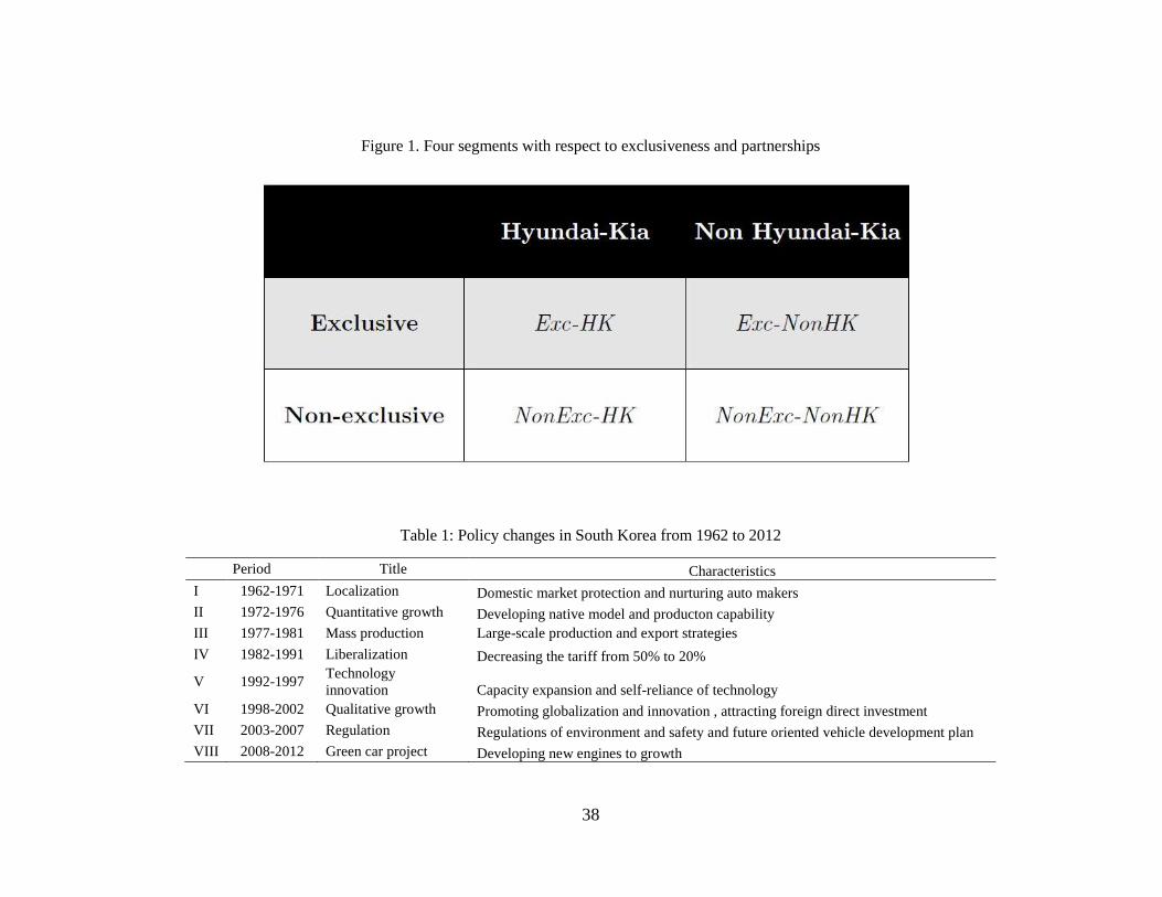
I divide automotive parts suppliers into four segments by the level of knowledge trans-

ferability. As a proxy for knowledge transferability, two network measures, exclusiveness

and the identity of the partnerships, are used. exclusiveness is defined as suppliers who

have one partner to trade. The four segments are the exclusive with Hyundai-Kia segment

(Exc-HK ), the exclusive with Non Hyundai-Kia segment (Exc-NonHK ), the non-exclusive

with Hyundai-Kia segment (NonExc-HK ), the non-exclusive with Non Hyundai-Kia segment

(NonExc-NonHK ). As the market size of all four increases, the market concentration moves

in different directions for each segment. The data set shows a non-monotonic relationship

for the NonExc-HK segment and a monotonic relationship for the NonExc-NonHK segment.

If the patterns were consistent with Sutton’s insights, suppliers in the NonExc-HK segment

would focus more on the quality-sensitive products, and the Nonexc-NonHK segments are

more likely to produce homogeneous products.

The component-related data allows me to capture the component distribution in each

segment. I find the results are consistent with Sutton’s insights. Automotive parts suppliers

in the NonExc-HK segment produce more technology-oriented products such as steering,

and power generating systems. NonExc-NonHK segment are more likely to produce less

quality-sensitive products such as lamps, and parts (aluminum). I also find that the exclusive

segments produce more design-oriented products such as molding and leather.

3The number of suppliers did not change over time. There were 878 suppliers in 2003 and 794 in 2008.

3

Second, I test the stability of the supply chain networks by the observed networks of the

Korean automobile supply chain in two different time periods. Theoretically, the substitute

conditions are crucial to guarantee the existence of pair-wise stable allocations (Hatfiled

and Milgrom, 2005; Halfield and Kominers 2010). However, the substitutes do not hold for

automotive suppliers. Hatfield and Kojima (2008) show that stable allocation may exist even

if contracts are not substitutes. A naturally arising question is then whether it is possible

to test the stability of networks empirically. The stability of the supply chain is based on

the long-term relationship between automotive parts suppliers and automobile assemblies.

However, there is no existing literature to test the stability of supply chain networks in the

automobile industry due to the inability of data set. The observed network data from two

time periods, 2008 and 2013 allow me to measure the distance of two networks and test the

stability. Since networks structures can be defined by adjacency matrices, distance measures

should be based on the graph spectra. The distance measures, which I use, are the eigenvalue

approach of the Laplacian matrix. The Laplacian matrix is defined as the difference between

the degree matrix and the adjacency matrix. To test stability, I calculate eigenvalues of the

normalized Laplacian matrix of two network structures in 2008 and in 2013 and then derive

the distance measures. The measures show that the supply chain networks in the Korean

automobile industry are very stable.

Third, I estimate the effects of network measures on automotive suppliers’ R&D invest-

ments using panel data. I define the network measures to capture the information flow

between upstream and downstream firms and among upstream firms: the degree with length

1, the degree with length 2, the number of competitors, and exclusiveness. In the panel

data analysis, a main concern is the unobservable firm-heterogeneity. If the unobservable

firm-heterogeneity were correlated with regressors, the OLS results would be biased and in-

consistent. The fixed effects estimator cannot be used here since all the network measures are

time-invariant due to the stability of network structures. I applied the Fixed Effects Filtered

(FEF) estimator (Pesaran and Zhou, 2013) to estimate both time-variant and time-invariant

4

regressors consistently with the correct covariance matrix. The Hausman and Taylor (HT)

estimator is considered but cannot be identified due to the restrictions of the data set. The

results show that exclusiveness and the level of price competition play an important role

concerning the level of investment committed to R&D.

This paper contributes to three strands of the literature. The first contribution addresses

the role of endogenous sunk costs on the relationship between market structure and market

concentration (Sutton, 1991). Empirical analysis has been done for different industries:

newspapers and restaurant industry (Berry and Waldfogel, 2010), the supermarket industry

(Ellickson, 2007, 2013) and the mutual fund industry (Gavazza, 2011; Park, 2013). In the

U.S. mutual fund industry, Park (2013) divides the exogenous sunk costs market and the

endogenous sunk costs market by segments with and without loads and Gavazza (2011) uses

the retail and institutional funds industry.

Second, this paper contributes to empirical literature on networks. Estimating the net-

work effects is related to measurement issues because it is not obvious how networks should

be measured. Typically defining the network is simply defining the neighborhood. For exam-

ple, in the early development literature, the village level had been used as the best possible

measure of networks (Munshi and Myaus, 2006, Munshi, 2004, Foster and Resenzweig, 1995)

and specific questions to determine the relationships are often included in the experiments

(Conley and Udry, 2010). However, research on networks effects among firms has been lim-

ited due to the availability of data. This paper empirically estimates the network effects

on suppliers’ R&D investment decisions under the supply chain structure. The uniqueness

of this data allows me to define various measures to capture the network effects between

automotive parts suppliers and automobile assemblies as well as among parts suppliers. In

addition, I directly test the sustainabilty of the supply chain. The theoretical analysis fo-

cuses on the conditions to obtain a pair-wise stability in the supply chain (Ostrovsky, 2008;

Hatfield and Kominers, 2012). Same-side substitutability and cross-side complementarity are

the main conditions to guarantee stable allocations and the automobile industry is a typical

5

example that does not satisfy the substitutability condition. Hatfield and Kojima (2008)

show that stable allocation may exist even if contracts are not substitutes but a weaker form

of substitutability is necessary. Fox (2010)’s work uses the maximum score estimator.

This study also contributes to the empirical literature on R&D investment. Belderbos et

al. (2006) test if R&D cooperations with different types of partners are complements using the

definition of complementarity by Milgrom and Roberts (1990). They find empirical evidence

of complementarities from joint cooperation strategies with competitors and customers and

with customers and universities.

The article is organized as follows: Section 2 explains the Korean automotive industry and

Section 3 describes the data set. In Section 4, connections between theoretical implications

and empirical patterns are considered. Section 5 tests the stability of supply chain and

Section 6 defines the network measures and discusses empirical strategy. Section 7 analyzes

the results. Finally, Section 8 concludes.

2 Korean Automobile Industry

In this section, I describe characteristics of downstream firms and upstream firms in the

Korean automobile industry. Historical policy changes are explained to shed light on the

structure of the Korean automobile industry.

2.1 Downstream Firms

Downstream firms in the automobile market are defined as automobile assemblers who

buy parts or components from upstream firms, assemble them to produce vehicles, and sell

to consumers. BMW, Toyota and Hyundai are examples of downstream firms. In the Ko-

rean automobile market, there are six automobile assemblers: Hyundai, Kia, GM Korea,

Renault Samsung, Ssangyong, and Tata Daewoo. A distinguishing characteristic of the Ko-

rean domestic automobile market is that domestic auto brands dominate the market. By

6

2012, Hyundai accounted for 44.6%, Kia for 33.5%, GM Daewoo for 9.5%, Renault Samsung

for 7.4% and Ssangyong for 2.6% of the market. In other words, all other foreign brands

including BMW, Honda, Toyota, Mercedes, Audi, and Nissan accounted for only 2.4% of the

Korean domestic market. The government had supported the domestic automobile market es-

pecially until 1980 in order to increase regional growth and employment of the middle class.

The stable domestic market share has helped domestic automobile assemblers to enhance

competitiveness in the international market. To analyze the downstream firms in Korea,

historical facts are important. The current Korean automobile market structure changed

tremendously after the 1997 Asian Financial Crisis. Before 1997, Hyundai, Kia, Daewoo,

Samsung and Ssangyong were domestic automobile companies. Kia had financial troubles,

and Kia Motors declared bankrupcy in 1997 and acquired 51% of the assets. Currently, 32%

of Kia is owned by Hyundai. Kia Motors is considered as a subsidiary of Hyundai Motors.

Daewoo Motors ran into financial problems and sold to General Motors. Daewoo Commer-

cial Vehicle Company was separated from parent Deawoo Motors and was acquired by Tata

Motors. Samsung Motors has been a subsidiary of Renault and changed its name to Renault

Samsung Motors from 2000. Ssangyong Motor was acquired by Tata Daewoo in 1997, sold to

Chinese automobile manufacturer SAIC in 2004 and then, to Indian Mahindra and Mahindra

Limited in 2011.

Hyundai-Kia vs. Non Hyundai-Kia Korean automobile companies can be divided

into two groups: (1) Hyundai and Kia and (2) GM Daewoo, Renault Samsung, SsangYong

and Tata Daewoo by two criteria: foreign ownership and market power. First, the Korean

automobile manufacturers except for Hyundai and Kia were acquired by foreign automobile

manufacturers. Domestic or foreign ownership is important to decide the level of R&D

investments conducted in Korea. Hyundai-Kia has to design and produce their own models

while foreign-owned automobile companies do not need to and instead, focus on licensing

vehicle models from GM and Renault. Second, there is a big difference between the two

groups from the viewpoints of the market share. If Hyundai and Kia were considered as one

7

company, the market share of Hyundai and Kia would be 78.1% and a summed market share

of the four is less than 20%. Naturally, downstream firms have more power than upstream

firms by the characteristics of the producer-driven supply chain in the automotive industry.

The difference of the market share would affect the power in negotiations with automotive

parts suppliers. Naturally, downstream firms have more power than upstream firms by the

characteristics of the producer-driven supply chain in the automobile industry.

2.2 Upstream Firms

Upstream firms are defined as automotive parts suppliers who produce parts or components

such as airbags and brake pedals and sell them to downstream firms which are automobile

assemblers. Historically, upstream firms were developed under vertically integrated frame-

works when the automobile industry started. Automobile assemblies provided automotive

parts suppliers with the blueprint including the details of technically sensitive information.

Thus many features of upstream firms have been developed according to the identity of part-

nerships. Automobile assemblies rather than automotive parts suppliers are the primary

investors in R&D. $2.46 billion which accounts for 67.5% 4 was invested by 5 automobile

assemblies in 2008.

2.3 Policy Changes

Historical policy changes over the previous six decades explain the structural development

of the Korean automobile industry. It is possible to divide this development into 8 periods

based on the political circumstances. Table 1 summarizes changes in the Korean automotive

industry from 1962 to 2012. Lee (2012) divided this period into two identifiable time frames,

“Protection and rationalization” from Period I to Period III and “Globalization, innovation

and regulation” from the Period IV to Period VIII.

Period I, 1962-71 was “Localization”. The goal of the Korean government is to protect

4Total amounts of R&D expenditure in the Korean automotive industry is $3.5 billion.

8

the domestic market and nurture domestic auto makers. To overcome a lack of knowledge

and know-how in producing vehicles, auto makers were encouraged to sign technical licensing

agreements with advanced foreign auto companies. As a tool of domestic market protection,

operations of foreign auto makers were banned except for joint ventures. A low level of

exchange rates, interest rates and oil prices had positive effects on the speed of localization.

Period II, from 1972 to 1976, was a time of “Quantitative growth” which focused on

developing native models and production capability. Economy of scale and scope was used

by the long-term growth plan. In addition, the government supported vertical integration

and cooperation. In 1974, the government announced its “Long-term automotive industry

promotion plan,” which promoted cooperation between parts and assembly industries, and

in 1975, it designated 35 vertically integrated parts producing facilities. These systematic

supports in favor of a stable relationship between automotive parts suppliers and automobile

assemblies were the main source of the current stability of the supply chain in the Korean au-

tomotive market. Period III, 1977-1981 can be called “Mass production and specialization”;

it established large-scale production and export strategies.

From Period IV, the focus had moved from protection to liberalization. Period IV, from

1982 to 1991, was “Liberalization” to change from government-led growth to private-initiated

growth with higher competition. Prior to 1987, foreign car makers were prohibited from

selling vehicles in Korea. From 1987, they were permitted to sell vehicles larger than 2000

cc and from 1988 on, they were allowed to make all types of cars. The domestic market had

been protected by a high level of tariffs, 50% by 1987, which gradually decreased to 20% in

1990 as a result of liberalization.

Period V, 1992-1997, was “Technology innovation” in which Korean automakers expanded

and became self-reliant in terms of technology. There were big changes before and after the

1997 Asian financial crisis. By the IMF’s instruction, globalization occurred rapidly during

Period VI, 1998-2002, and qualitative growth was achieved. Period VII, 2003-2007, was

represented by the environmental and safety related regulations and future-oriented vehicle

9

development plans. The ”Green car project” explains the Period VIII, 2008-2012, which

developed new engines to stimulate growth.

3 Data

The panel data used in this paper has been constructed from three sources of data sets by

matching automotive parts suppliers’ identity. Each data set is used for a different purpose.

The first data set allows me to estimate the network structures of the Korean automotive

industry, shown in Figure 1. It reveals the linkages between 892 automotive parts suppliers

and 6 automobile assembly companies in 2008. The information about the linkages allows

researchers to define the networks measures between upstream and downstream firms and

among upstream firms. A percentage share for each automobile assembly company for each

automotive parts supplier can be identified. This data is available only for 2008 and 2013. In

Section 5, to test the stability of networks, I used both years’ observations. The estimation

procedures of Section 6 and Section 7 use the data in 2008.

The second data set contains 480 automotive parts suppliers from 1999 to 2010. The data

set has been constructed from annual financial reports using the DART (Data Analysis, Re-

trieval and Transfer) system of Financial Supervisory Service. It consists of the total revenue,

profit, total liability, equity, capital, current assets, current liability, R&D investment, and

number of employees. Filing disclosure documents on main events is mandatory for listed

corporations in the KRX or the KOSDAQ or for companies whose capital assets exceed $7

million based on the previous year.

The third data set is component-related information which offers important information

for two purposes. I can investigate the consistency by using the distribution of components

in Section 4. In Section 6 and Section 7, component information is used as control variables.

As Figure 2 shows, the supply chain structure is extremely complicated. The key trick to

simplify the structure is to consider the supply chain with respect to each component. For

10

example, there are 7 suppliers to produce the air cleaners press type. As Figure 3 shows, the

relationship is more simply observable and the market can be seen as a two-sided market.

The data includes which parts are produced by 480 suppliers. Since there are more than

50,000 components, the information is grouped into 378 different components. By combining

this with the second data set, I can identify which components are produced by each supplier.

I projected 378 parts on two different spaces. The first space is categorized by materials and

the second space focuses on the use of the automotive parts in the vehicle. The first space

contains 21 categories and the second does 11. For example, I can map oil pump as “pump”

in the first standards of categorization and “power generating and transfer system” by the

second standards as Figure 5 shows.

The limitation is that we are unable to capture the financial variables such as profit by

each part when a supplier produces more than one automotive part. During the process to

combine the first and second data set, I exclude parts suppliers who sell their parts to the

other parts suppliers. In other words, the sample includes only first-tier suppliers who have

partnerships with automobile assemblies. Lee (2010) said that there are more than 2000

second-tier suppliers but it is difficult to observe them by the data set. This is because the

customers of second-tier suppliers vary across the industry. Products of second-tier suppliers

are raw or intermediate material of automotive parts as well as materials in other industries.

Finally, my data set consists of 334 first-tier automotive parts suppliers from 1999 to

2010. Thus, the total number of observations is 4008. In the firm analysis, firms’ birth and

death are one of the most important issues. In the automotive industry, it seems that the

birth and death of suppliers would not be a problem. Table 2 shows the number of suppliers

who enter and exit each year, and we have already excluded firms that do not sell parts to

the automobile assembly companies. In the empirical analysis, I used the balanced panel

data. The number of firms is 334 since it is calculated by (i)-(ii)-(iii)+(iv)-(v) in Table 3.

11

4 Theory and Empirical Patterns

In this section, I discuss how empirical patterns are consistent with Sutton (1991)’s endoge-

nous sunk costs model. Corchon and Wilkie (1994) explain asymmetry of R&D behaviors.

4.1 Theoretical Implications

Sutton (1991) studies two analytical frameworks5, exogenous sunk costs and endogenous

sunk costs to show the relationship between market size and market concentration. A major

difference between the exogenous sunk costs model and the endogenous sunk costs model

centers around the role of fixed outlays in sunk costs in determining the consumers’ willingness

to pay.

The exogenous sunk cost model is the two-stage game. The first stage is the entry decision.

Firms enter the market if the net profit, Π, is greater than the sunk costs for setting up, σ.

The number of firms, N, is determined in this stage.

Π ≥ σ

The second stage is the Cournot competition. Given the number of firms, N, the level of

price and quantity are determined by maximizing their profit.6 The model yields the following

equation:

N∗ =

√S

σ

The main implication of the exogenous sunk costs model is a monotonic relationship between

the market size and the market concentration. As the market size increases, the market

becomes more competitive.

The endogenous sunk costs model consists of three stages. The first stage is the entry

5In considering the theoretical implications, I only include examples of the Cournot competition. Detailsand other cases such as the Bertrand competition are discussed in Sutton’s book. Both exogenous andendogenous sunk costs models are solved by backwards induction.

6The demand schedule is X = S/p, and firm i’s profit, Π = pi(∑xj)xi − cxi

12

decision. Firms determine to enter the market if the net profit exceeds the sunk costs.

The difference is that the sunk costs contain two elements: the set up cost, σ, and R&D

investment, A(u).

Π(u) ≥ F (u) = σ + A(u).

At the second stage, given the number of firms, firms determine the quality level, u, by the

first-order condition. Then, the levels of R&D or advertising are determined by the response

function, A(u)7

dΠ

du|u=u −

dF

du|u=u ≤ 0 and u ≥ 1 w.complementaryslackness

The third stage is the Cournot Competition8.

N +1

N− 2 =

γ

2[1− σ − a/γ

SN2].

The main implications of the endogenous sunk costs model are that a non-monotonic

relationship between the market size and the market concentration can be found according

to the value of σ and a/γ. In the R&D or advertising-intensive industry in which endogenous

elements in sunk costs are associated with consumers’ preference, the market concentration

can even increase as the market size increases.

From 1999 to 2010, the market size of the automotive parts industry increased as measured

by sales. As the market size increased, the number of automotive parts suppliers remained

the same. There were 881 parts suppliers in 2001 and 898 in 2013. This non-monotonic

relationship implies that the Korean automobile market is more likely to be an instance of

endogenous sunk costs. However, the R&D investments patterns of automotive parts suppli-

ers are not consistent with Sutton’s model. The automotive parts industry does not seem to

7A(u) is a convex smooth function on the domain u ≥ 1 and A(1) = 1. In Sutton’s example, A(u) =aγ (uγ − 1), γ > 1

8ui/pi = uj/pj is derived by the consumer’s problem to maximize U = (ux)γz1−γ subject to pixi+pz+z ≤M where x is the good in interest, z is outside good, and u is the index of perceived quality. The demandschedule is X = S/p and profit is Π = pi(

∑xj)xi − cxi.

13

be R&D intensive. To think about this paradox, I will focus on knowledge transferability in

Section 5 with empirical patterns.

Asymmetry of R&D behavior Corchon and Wilkie (1994) model the sources of the

productivity paradox in which investments in a new technology have not led to a general

increase in productivity. The model consists of two stages based on the traditional Cournot

model with a discrete change of technology. Technology consists of a fixed capital cost, f , and

a variable cost, c. The initial production technology is T0 = (f0, c0) and the new technology

is T1 = (f1, c1), where f1 > f0, c1 < c0. The setting implies that more investments in R&D

can decrease suppliers’ variable costs. By the Cournot competition9, the following three

conditions can be derived:

(1) A firm will innovate if and only if

{a+ (n− 1)c0 − nc1

n+ 1}2 − {a− c0

n+ 1}2 > f1 − f0

(2) Each firm invests in the new technology if

{a− c1

n+ 1}2 − {a+ (n− 1)c1 − nc0

n+ 1}2 ≥ f1 − f0

(3) A sufficient condition for productivity to fall

f1 − f0 > (c0 − c1){a− c1

n+ 1}

Corchon and Wilkie find that when a−c1c0−c1 ≥

n2

n−1, then for some values of f1 − f0 the

productivity paradox will occur. They show that if the second equation holds, then the sym-

metric equilibrium is the unique subgame perfect equilibrium of the game (SPNE). Hyundai

and Kia invest in R&D but the four other assemblies rarely commit to R&D investments in

Korea. The current automobile market is far from being an instance of symmetric equilib-

9Firms compete to maximize the profit. Profit is Πi(q, f0, c0) = D(Q)qi− c0qi− f0. The demand curve isnormalized linear and total factor productivity is defined as the inverse of summation of average costs.

14

rium. To understand an asymmetric case, I need to consider the meaning that equation (2)

does not hold. Equation (2) is the condition that all firms invest in a new technology. When

the leading firm introduces the new technology10, the firm can enjoy the profit and an increase

in market share. Then, as more firms adopt the new technology, a high level of competition

erodes market share. Since fixed costs in investing in R&D have to be spread between firms,

the productivity paradox can occur. In the Korean automobile industry, Hyundai and Kia

adopted the technology earlier than the other assemblies and increased their market share.

When the other assemblies adopt the new technology, their productivity may not increase

due to increased competition and to a high level of fixed costs which spread to a small market

share. Then, during the 1997 Asian financial crisis, they were acquired by foreign companies.

4.2 Empirical Patterns

To find evidence from empirical patterns, I define the knowledge transferability by two

network measures: exclusiveness and the identity of partnerships as the first step. Then, I

divide four segments with respect to two measures. Second, I analyze dynamic patterns of

market size, market structures and R&D within each segment. Patterns suggest that the

size of fixed outlays in sunk costs is determined by knowledge transferability. If patterns

are consistent with Sutton’s insights, the segment which has a higher level of endogeneity

in sunk costs, should be more quality-sensitive. As the final step, I show the distribution of

components in each segment.

Knowledge Transferability Since knowledge is not visible, measuring the knowledge

transferability is the first empirical issue. To find an adequate proxy of knowledge transfer-

ability, I used two measures: exclusiveness and the identity of partnerships.

Exclusiveness is defined as the suppliers having only one partnership with an automobile

assembly. Exclusiveness represents a higher level of knowledge transferability from automo-

bile assemblies to automotive parts suppliers. This is because automobile assemblies tend

10Their results show that a monopolist introduce the new technology if and only if the new technologyraises total factor productivity and the equation (2) implies the equation (1)

15

to be less concerned that technologically sensitive information will spread to their rivals.

Knowledge transferability based on exclusiveness allows internal R&D and external R&D to

be substitutes.

The identity of partnerships is defined as Hyundai-Kia (HK) and Non Hyundai-Kia

(NonHK). Hyundai and Kia have distinguishing characteristics from the four other assemblies

(GM Korea, Renault Samsung, Ssangyong, and Tata Daewoo) based on two criteria: foreign

ownership and market power. Having a partnership with Hyundai and Kia determines a

higher level of knowledge transferability because Hyundai and Kia are the only companies

to conduct R&D in Korea. The four other automobile assemblies were acquired by foreign

automobile manufacturers and focus more on licensing vehicle models. For example, GM

Korea licenses the model from General Motors and R&D of General Motors is conducted in

the U.S. 73.35% of patents have been made by Hyundai and Kia in Korea, which is consistent

with R&D patterns. The market share of Hyundai and Kia is 78.1% if the two companies

are considered as one company and a summed market share of the four other assemblies is

less than 20%.

According to two measures of the level of knowledge transferability, I divide automotive

parts suppliers into four segments as follows:

(1) Exclusive with Hyundai-Kia segment (Exc-HK ): High-High

(2) Exclusive with non Hyundai-Kia segment (Exc-NonHK ): High-Low

(3) Non-exclusive with Hyundai-Kia segment (NonExc-HK ): Low-High

(4) Non-exclusive with non Hyundai-Kia segment (NonExc-NonHK ): Low-Low

The Exc-HK segment has the highest level of knowledge transferability and the NonExc-

NonHK segment has the lowest level of knowledge transferability. Exclusiveness has a

higher level of knowledge transferability than non-exclusiveness and having a partnership

with Hyundai-Kia has a higher level than not having a partnership with Hyundai-Kia. Anal-

16

ysis with respect to segments provides us with interesting insights.

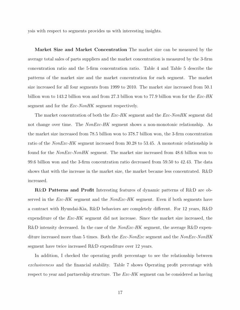
Market Size and Market Concentration The market size can be measured by the

average total sales of parts suppliers and the market concentration is measured by the 3-firm

concentration ratio and the 5-firm concentration ratio. Table 4 and Table 5 describe the

patterns of the market size and the market concentration for each segment. The market

size increased for all four segments from 1999 to 2010. The market size increased from 50.1

billion won to 143.2 billion won and from 27.3 billion won to 77.9 billion won for the Exc-HK

segment and for the Exc-NonHK segment respectively.

The market concentration of both the Exc-HK segment and the Exc-NonHK segment did

not change over time. The NonExc-HK segment shows a non-monotonic relationship. As

the market size increased from 78.5 billion won to 378.7 billion won, the 3-firm concentration

ratio of the NonExc-HK segment increased from 30.28 to 53.45. A monotonic relationship is

found for the NonExc-NonHK segment. The market size increased from 48.6 billion won to

99.6 billion won and the 3-firm concentration ratio decreased from 59.50 to 42.43. The data

shows that with the increase in the market size, the market became less concentrated. R&D

increased.

R&D Patterns and Profit Interesting features of dynamic patterns of R&D are ob-

served in the Exc-HK segment and the NonExc-HK segment. Even if both segments have

a contract with Hyundai-Kia, R&D behaviors are completely different. For 12 years, R&D

expenditure of the Exc-HK segment did not increase. Since the market size increased, the

R&D intensity decreased. In the case of the NonExc-HK segment, the average R&D expen-

diture increased more than 5 times. Both the Exc-NonExc segment and the NonExc-NonHK

segment have twice increased R&D expenditure over 12 years.

In addition, I checked the operating profit percentage to see the relationship between

exclusiveness and the financial stability. Table 7 shows Operating profit percentage with

respect to year and partnership structure. The Exc-HK segment can be considered as having

17

the most stable sources of profits from Hyundai-Kia since the standard error is the lowest

among four segments. Suppliers in the Exc-NonHK segment are most affected by financial

fluctuations. When economic conditions are good, their operating profit percentages are

greater than the profit percentage of suppliers in the Exc-HK segment. However, their profit

percentages were even negative in 1999 and 2009.

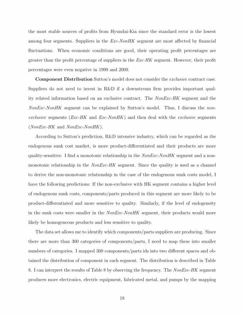
Component Distribution Sutton’s model does not consider the exclusive contract case.

Suppliers do not need to invest in R&D if a downstream firm provides important qual-

ity related information based on an exclusive contract. The NonExc-HK segment and the

NonExc-NonHK segment can be explained by Sutton’s model. Thus, I discuss the non-

exclusive segments (Exc-HK and Exc-NonHK ) and then deal with the exclusive segments

(NonExc-HK and NonExc-NonHK ).

According to Sutton’s prediction, R&D intensive industry, which can be regarded as the

endogenous sunk cost market, is more product-differentiated and their products are more

quality-sensitive. I find a monotonic relationship in the NonExc-NonHK segment and a non-

monotonic relationship in the NonExc-HK segment. Since the quality is used as a channel

to derive the non-monotonic relationship in the case of the endogenous sunk costs model, I

have the following predictions: If the non-exclusive with HK segment contains a higher level

of endogenous sunk costs, components/parts produced in this segment are more likely to be

product-differentiated and more sensitive to quality. Similarly, if the level of endogeneity

in the sunk costs were smaller in the NonExc-NonHK segment, their products would more

likely be homogeneous products and less sensitive to quality.

The data set allows me to identify which components/parts suppliers are producing. Since

there are more than 300 categories of components/parts, I need to map these into smaller

numbers of categories. I mapped 300 components/parts ids into two different spaces and ob-

tained the distribution of component in each segment. The distribution is described in Table

8. I can interpret the results of Table 8 by observing the frequency. The NonExc-HK segment

produces more electronics, electric equipment, fabricated metal, and pumps by the mapping

18

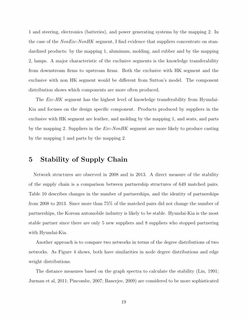
1 and steering, electronics (batteries), and power generating systems by the mapping 2. In

the case of the NonExc-NonHK segment, I find evidence that suppliers concentrate on stan-

dardized products: by the mapping 1, aluminum, molding, and rubber and by the mapping

2, lamps. A major characteristic of the exclusive segments is the knowledge transferability

from downstream firms to upstream firms. Both the exclusive with HK segment and the

exclusive with non HK segment would be different from Sutton’s model. The component

distribution shows which components are more often produced.

The Exc-HK segment has the highest level of knowledge transferability from Hyundai-

Kia and focuses on the design specific component. Products produced by suppliers in the

exclusive with HK segment are leather, and molding by the mapping 1, and seats, and parts

by the mapping 2. Suppliers in the Exc-NonHK segment are more likely to produce casting

by the mapping 1 and parts by the mapping 2.

5 Stability of Supply Chain

Network structures are observed in 2008 and in 2013. A direct measure of the stability

of the supply chain is a comparison between partnership structures of 649 matched pairs.

Table 10 describes changes in the number of partnerships, and the identity of partnerships

from 2008 to 2013. Since more than 75% of the matched pairs did not change the number of

partnerships, the Korean automobile industry is likely to be stable. Hyundai-Kia is the most

stable partner since there are only 5 new suppliers and 8 suppliers who stopped partnering

with Hyundai-Kia.

Another approach is to compare two networks in terms of the degree distributions of two

networks. As Figure 4 shows, both have similarities in node degree distributions and edge

weight distributions.

The distance measures based on the graph spectra to calculate the stability (Lin, 1991;

Jurman et al, 2011; Pincombe, 2007; Banerjee, 2009) are considered to be more sophisticated

19

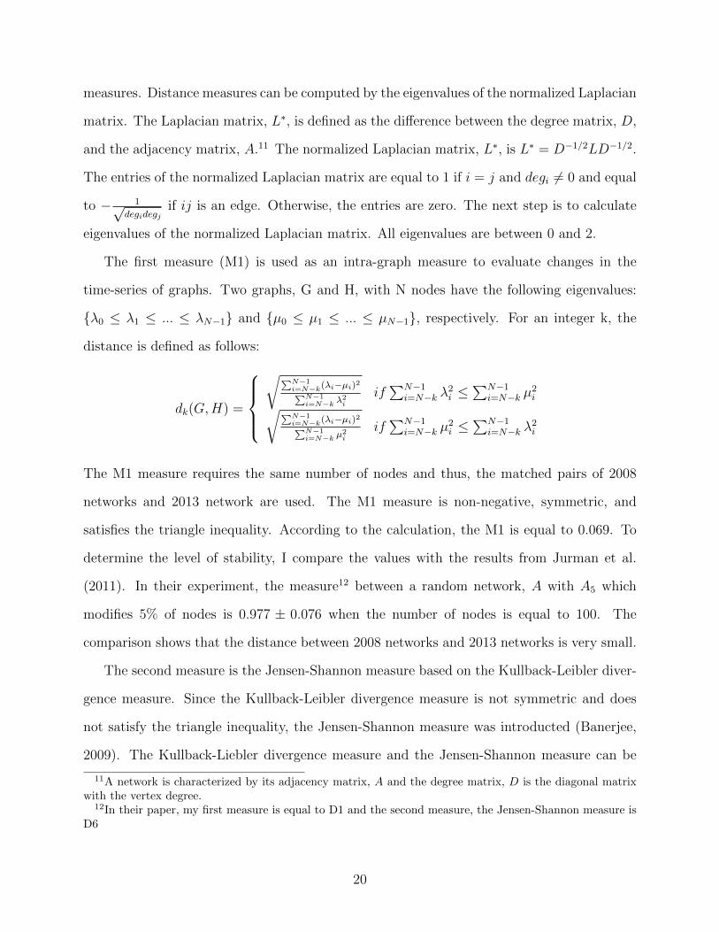
measures. Distance measures can be computed by the eigenvalues of the normalized Laplacian

matrix. The Laplacian matrix, L∗, is defined as the difference between the degree matrix, D,

and the adjacency matrix, A.11 The normalized Laplacian matrix, L∗, is L∗ = D−1/2LD−1/2.

The entries of the normalized Laplacian matrix are equal to 1 if i = j and degi 6= 0 and equal

to − 1√degidegj

if ij is an edge. Otherwise, the entries are zero. The next step is to calculate

eigenvalues of the normalized Laplacian matrix. All eigenvalues are between 0 and 2.

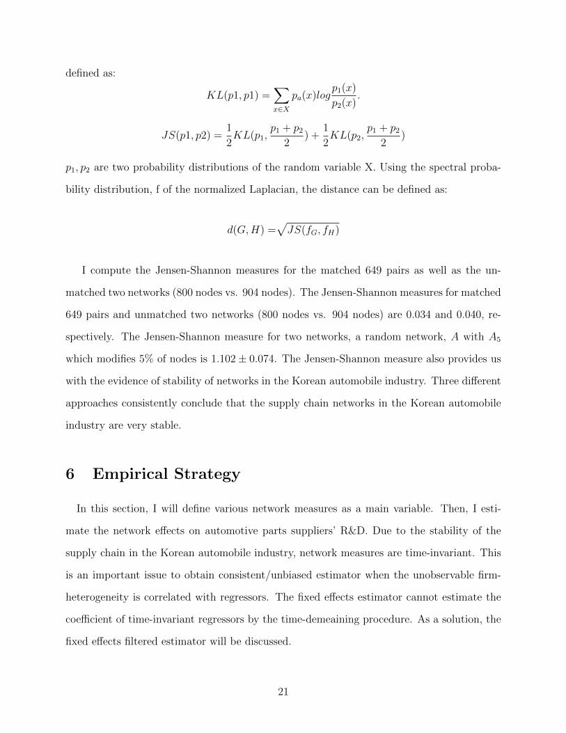
The first measure (M1) is used as an intra-graph measure to evaluate changes in the

time-series of graphs. Two graphs, G and H, with N nodes have the following eigenvalues:

{λ0 ≤ λ1 ≤ ... ≤ λN−1} and {µ0 ≤ µ1 ≤ ... ≤ µN−1}, respectively. For an integer k, the

distance is defined as follows:

dk(G,H) =

√∑N−1

i=N−k(λi−µi)2∑N−1i=N−k λ

2i

if∑N−1

i=N−k λ2i ≤

∑N−1i=N−k µ

2i√∑N−1

i=N−k(λi−µi)2∑N−1i=N−k µ

2i

if∑N−1

i=N−k µ2i ≤

∑N−1i=N−k λ

2i

The M1 measure requires the same number of nodes and thus, the matched pairs of 2008

networks and 2013 network are used. The M1 measure is non-negative, symmetric, and

satisfies the triangle inequality. According to the calculation, the M1 is equal to 0.069. To

determine the level of stability, I compare the values with the results from Jurman et al.

(2011). In their experiment, the measure12 between a random network, A with A5 which

modifies 5% of nodes is 0.977 ± 0.076 when the number of nodes is equal to 100. The

comparison shows that the distance between 2008 networks and 2013 networks is very small.

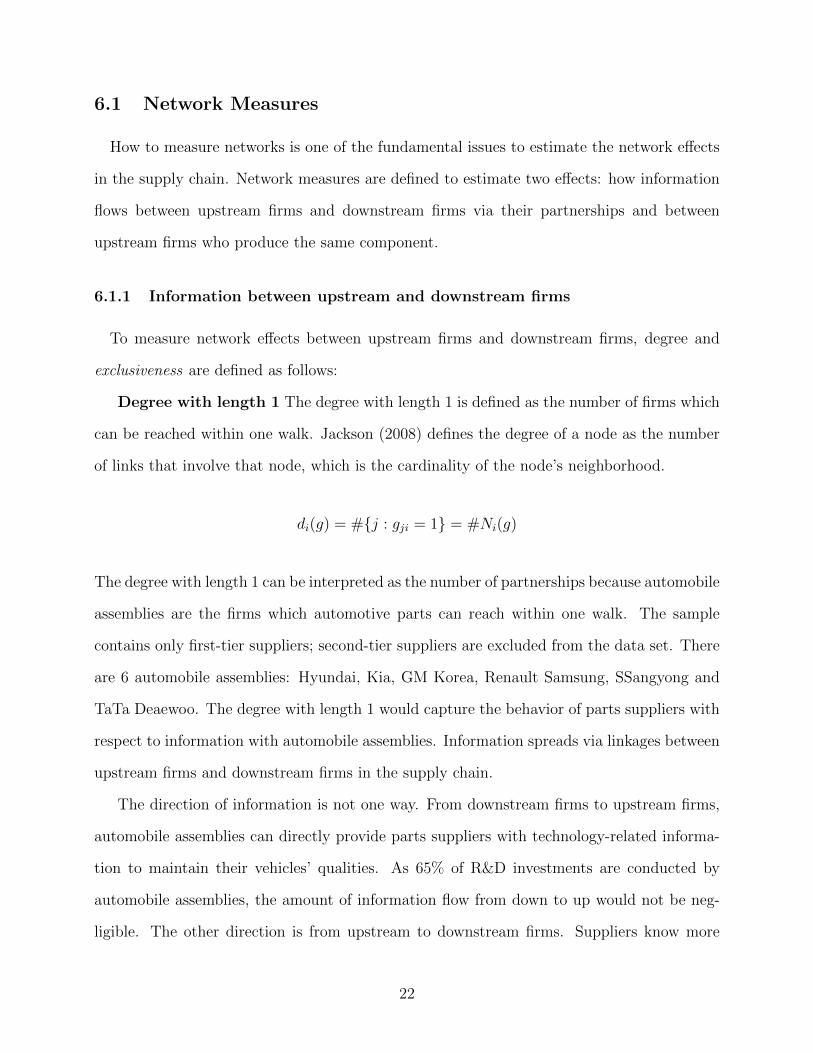
The second measure is the Jensen-Shannon measure based on the Kullback-Leibler diver-

gence measure. Since the Kullback-Leibler divergence measure is not symmetric and does

not satisfy the triangle inequality, the Jensen-Shannon measure was introducted (Banerjee,

2009). The Kullback-Liebler divergence measure and the Jensen-Shannon measure can be

11A network is characterized by its adjacency matrix, A and the degree matrix, D is the diagonal matrixwith the vertex degree.

12In their paper, my first measure is equal to D1 and the second measure, the Jensen-Shannon measure isD6

20

defined as:

KL(p1, p1) =∑x∈X

pa(x)logp1(x)

p2(x).

JS(p1, p2) =1

2KL(p1,

p1 + p2

2) +

1

2KL(p2,

p1 + p2

2)

p1, p2 are two probability distributions of the random variable X. Using the spectral proba-

bility distribution, f of the normalized Laplacian, the distance can be defined as:

d(G,H) =√JS(fG, fH)

I compute the Jensen-Shannon measures for the matched 649 pairs as well as the un-

matched two networks (800 nodes vs. 904 nodes). The Jensen-Shannon measures for matched

649 pairs and unmatched two networks (800 nodes vs. 904 nodes) are 0.034 and 0.040, re-

spectively. The Jensen-Shannon measure for two networks, a random network, A with A5

which modifies 5% of nodes is 1.102± 0.074. The Jensen-Shannon measure also provides us

with the evidence of stability of networks in the Korean automobile industry. Three different

approaches consistently conclude that the supply chain networks in the Korean automobile

industry are very stable.

6 Empirical Strategy

In this section, I will define various network measures as a main variable. Then, I esti-

mate the network effects on automotive parts suppliers’ R&D. Due to the stability of the

supply chain in the Korean automobile industry, network measures are time-invariant. This

is an important issue to obtain consistent/unbiased estimator when the unobservable firm-

heterogeneity is correlated with regressors. The fixed effects estimator cannot estimate the

coefficient of time-invariant regressors by the time-demeaining procedure. As a solution, the

fixed effects filtered estimator will be discussed.

21

6.1 Network Measures

How to measure networks is one of the fundamental issues to estimate the network effects

in the supply chain. Network measures are defined to estimate two effects: how information

flows between upstream firms and downstream firms via their partnerships and between

upstream firms who produce the same component.

6.1.1 Information between upstream and downstream firms

To measure network effects between upstream firms and downstream firms, degree and

exclusiveness are defined as follows:

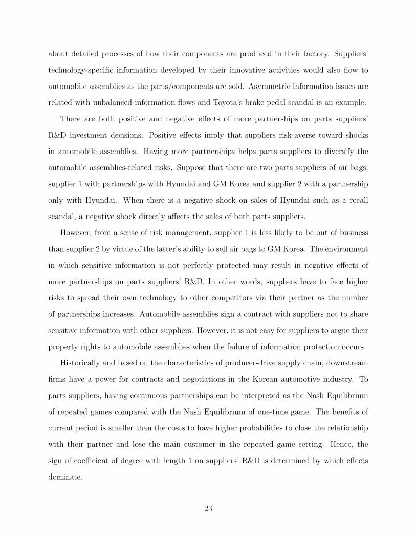
Degree with length 1 The degree with length 1 is defined as the number of firms which

can be reached within one walk. Jackson (2008) defines the degree of a node as the number

of links that involve that node, which is the cardinality of the node’s neighborhood.

di(g) = #{j : gji = 1} = #Ni(g)

The degree with length 1 can be interpreted as the number of partnerships because automobile

assemblies are the firms which automotive parts can reach within one walk. The sample

contains only first-tier suppliers; second-tier suppliers are excluded from the data set. There

are 6 automobile assemblies: Hyundai, Kia, GM Korea, Renault Samsung, SSangyong and

TaTa Deaewoo. The degree with length 1 would capture the behavior of parts suppliers with

respect to information with automobile assemblies. Information spreads via linkages between

upstream firms and downstream firms in the supply chain.

The direction of information is not one way. From downstream firms to upstream firms,

automobile assemblies can directly provide parts suppliers with technology-related informa-

tion to maintain their vehicles’ qualities. As 65% of R&D investments are conducted by

automobile assemblies, the amount of information flow from down to up would not be neg-

ligible. The other direction is from upstream to downstream firms. Suppliers know more

22

about detailed processes of how their components are produced in their factory. Suppliers’

technology-specific information developed by their innovative activities would also flow to

automobile assemblies as the parts/components are sold. Asymmetric information issues are

related with unbalanced information flows and Toyota’s brake pedal scandal is an example.

There are both positive and negative effects of more partnerships on parts suppliers’

R&D investment decisions. Positive effects imply that suppliers risk-averse toward shocks

in automobile assemblies. Having more partnerships helps parts suppliers to diversify the

automobile assemblies-related risks. Suppose that there are two parts suppliers of air bags:

supplier 1 with partnerships with Hyundai and GM Korea and supplier 2 with a partnership

only with Hyundai. When there is a negative shock on sales of Hyundai such as a recall

scandal, a negative shock directly affects the sales of both parts suppliers.

However, from a sense of risk management, supplier 1 is less likely to be out of business

than supplier 2 by virtue of the latter’s ability to sell air bags to GM Korea. The environment

in which sensitive information is not perfectly protected may result in negative effects of

more partnerships on parts suppliers’ R&D. In other words, suppliers have to face higher

risks to spread their own technology to other competitors via their partner as the number

of partnerships increases. Automobile assemblies sign a contract with suppliers not to share

sensitive information with other suppliers. However, it is not easy for suppliers to argue their

property rights to automobile assemblies when the failure of information protection occurs.

Historically and based on the characteristics of producer-drive supply chain, downstream

firms have a power for contracts and negotiations in the Korean automotive industry. To

parts suppliers, having continuous partnerships can be interpreted as the Nash Equilibrium

of repeated games compared with the Nash Equilibrium of one-time game. The benefits of

current period is smaller than the costs to have higher probabilities to close the relationship

with their partner and lose the main customer in the repeated game setting. Hence, the

sign of coefficient of degree with length 1 on suppliers’ R&D is determined by which effects

dominate.

23

Exclusiveness Exclusiveness is defined as the suppliers with only one partnership with

an automobile assembly.

ei(g) = 1 if di(g) = 1

= 0 otherwise

Exclusiveness is connected with downstream firms’ fears to spread their information via

linkages with suppliers. Automobile assemblies need to determine the level of technology-

intensive information flows from them to suppliers. Through the linkage of nonexclusive

suppliers with other automobile assemblies, sensitive information can be spread to their ri-

vals. As concerns the automobile assemblies increase, the contracts are more likely to be

exclusive. Exclusiveness is an important factor to decide if the technology is transferable or

not. Since Hyundai-Kia is different from the other 4 assemblies, the identity of the partner is

the next step in considering the transferability of technology. The data set shows that 45%

of the suppliers are exclusive and 69% of the exclusive suppliers (31%) have a partnership

with Hyundai-Kia.

6.1.2 Information flows among upstream firms

Degree with length 2 The degree with length 2 is the number of firms which can be

reached with two walks and captures the effect of how information flows via linkage among

parts suppliers. Mathematically, I can write it with the concept of an extended neighborhood

as follows:

d2i (g) = #N2

i (g)

N2i (g) = ∪j∈Ni(g)Nj(g)

The measure focuses on the network effect that sensitive information spreads to competitors

via supplier’s partnerships. The degree with length 2 is a similar concept with the number

24

of competitors which will be used as the network measure as well. However, the degree

with length 2 is smaller than or equal to the number of competitors since the degree is the

number of competitors which are connected with the supplier’s partners. Competitors are

defined as the firms who produce the same component. Because 73.5% of suppliers produce

more than one component, both the degree with length 2 and the number of competitors are

measured more than once with respect to the number of components. Thus, three measures

of degree are defined for extended neighborhood: minimum, average and maximum. The

summary statistics shows that minimum of degree with length 2 is 3.29 as the mean and

max and average are 9.30 and 5.72 respectively. If the share of each component in the sales

of suppliers, using the share as weights is one of the best way but it is not revealed. In the

empirical analysis, the minimum measure was used as a main variable of degree with length

2 because of decreasing marginal benefits of R&D with respect to the number of firms with

2 walks.

Number of Competitors Theory says that the entrants are less likely to enter the

market when price competition is tougher. The toughness of the price competition is an

important regressor but a difficult factor to observe in empirical analysis. Fortunately, the

number of firms which produce the same component can be a good proxy. The variable

is defined with respect to 378 components. In Figure 2, the number of competitors for air

cleaners (press type) is equal to 7. Since many companies produce more than one compo-

nent, minimum, maximum and average are calculated. For example, suppose supplier C

produces airbags and brake pedals. There are 2 competitors in airbag suppliers and 5 more

firms producing brake pedals. The measure of the average level of competition is equal to

4.5 as (3+6)/2, the minimum level is 3 and the maximum level is 6 respectively. The coeffi-

cient shows how suppliers respond to the R&D investment as the toughness of competition

changes. Both directions of sign are plausible. The coefficient is negative when suppliers are

less likely to invest in R&D since their new technology flows directly to their competitors

through the arrows between automotive parts suppliers and automobile companies. The sign

25

will be positive if the supplier tends to invest in R&D to survive in the highly competitive

environment. Empirical analysis will show whether the spillover effects dominate the compe-

tition effect or not. The correlation between individual firm’s productivity and the number

of competitors is related with the barriers to entry. If the incumbent sets the quality of the

product at the higher level, entrants will not be able to get into the market.

Characteristics of Components The characteristics of component-specific technology

is directly correlated with technology. Leather of seats and brake pedal system would require

a different level and sort of technology. Thus, controlling suppliers’ component characteristics

is essential to avoid the omitted variable bias. However, it is often impossible or neglected

due to limitations of the data.

6.2 Empirical Analysis

6.2.1 Econometric Issues

Now, I would like to estimate the effects of network measures on automotive parts sup-

pliers’ R&D decisions. The static model is constructed as follows:

yit = αi + xit′β + zi

′γ + uit

where i is the automotive part suppliers, i=1,2,...,N ; t is year, t=1,2,...,T.

The dependent variable, yit is each supplier’s R&D expenditure for individual firm i and

time t.

yit =J∑j=1

K∑k=1

ykijt

j is the automobile company; k is the automotive part. To control the size effects, R&D

expenditure is divided by two variables respectively: the total revenue or the number of

employees. xits are time-variant variables which represent the Performance in the Bain’s

26

paradigm: Profit, debt, current asset, total capital, current capital and current liability. zis

are time-invariant variables: the degree with length 1, the degree with length 2, the number

of competitors, the number of components, exclusiveness, the identity of the partnership, the

characteristics of component, union and areas. Summary statistics of dependent variable,

time-variant regressors and time-invariant regressors are given in Table 13. αi is defined as

αi = α + ηi and the unobservable firm-specific heterogeneity which does not vary over time.

In general, T is small, the pooled OLS is biased and inconsistent (Hsiao, 2003). If αi is

correlated with regressors, POLS is biased and inconsistent. The Fixed Effects estimator is

still consistent when αi is correlated with exogenous variables, xit. However, the weakness

of the Fixed Effects estimator is that the coefficients of time-invariant regressors are not

estimable. The time-invariant variables are eliminated by the demeaning procedure. This is

a serious problem since all the network measures are time-invariant due to the stability of

the supply chain. The econometrical question is the following: how can I estimate both time

variant and time-invariant regressors consistently even if there exists the correlation between

regressors and firm-specific heterogeneity? Hausman and Taylor estimator is a remedy to

use the concept of the instrumental variables but cannot be applied to my paper since the

restrictions are not satisfied. I will consider the Fixed Effects Filtered (FEF) estimator in

this paper which is shown to work well under various scenarios by Pesaran and Zhou (2013)13.

6.2.2 Fixed Effects Filtered Estimator

To estimate the coefficient of time-invariant variables consistently even if the firm-specific

heterogeneity is correlated with exogenous variables, I apply the Fixed Effects Filtered es-

timator. In this subsection, I discuss the fixed effects filtered estimator. The underlying

idea of FEF is straightforward and can be implemented in two step. The first step of FEF

estimator is to apply the FE estimation to get an estimator of β, which is consistent when N

13There is also so called Fixed Effects Vector Decomposition (FEVD) in the political science, as shown byPesaran and Zhou (2013), this FEVD estimator is identical to FEF estimator if an intercept is included inthe regressor, otherwise it is inconsistent in general. Refer to Pesaran and Zhou (2013) and Plumber andTroeger (2007) for more details.

27

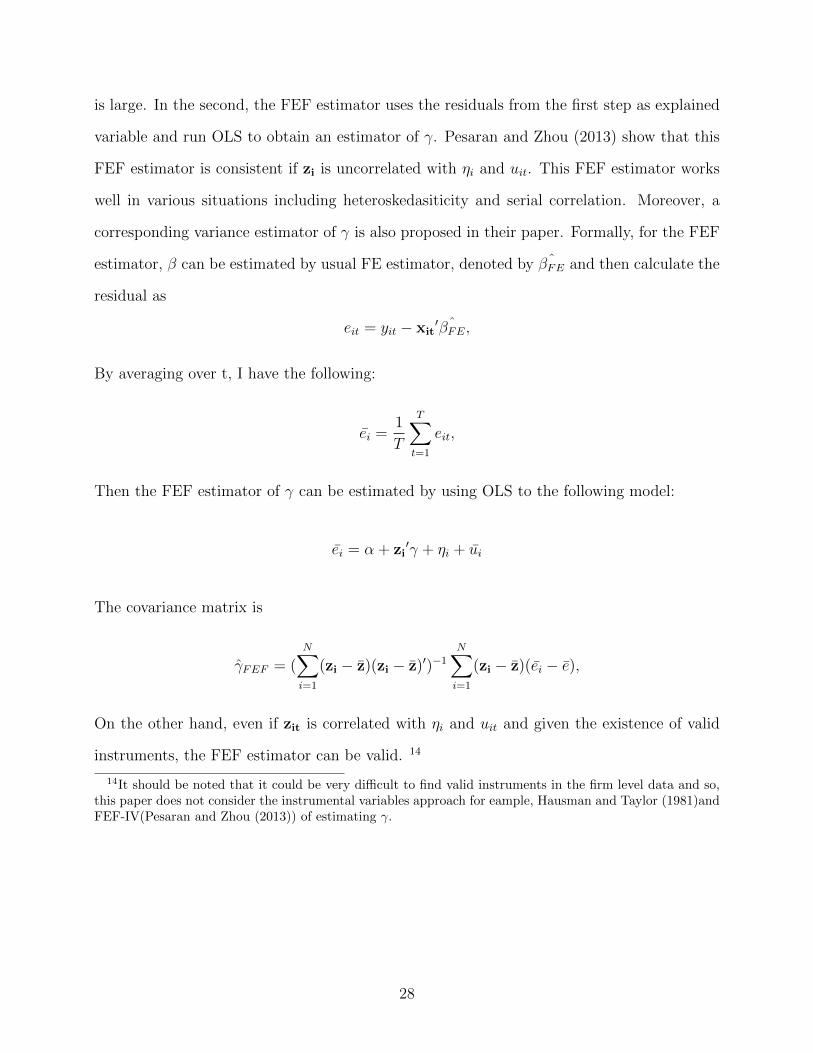
is large. In the second, the FEF estimator uses the residuals from the first step as explained

variable and run OLS to obtain an estimator of γ. Pesaran and Zhou (2013) show that this

FEF estimator is consistent if zi is uncorrelated with ηi and uit. This FEF estimator works

well in various situations including heteroskedasiticity and serial correlation. Moreover, a

corresponding variance estimator of γ is also proposed in their paper. Formally, for the FEF

estimator, β can be estimated by usual FE estimator, denoted by ˆβFE and then calculate the

residual as

eit = yit − xit′ ˆβFE,

By averaging over t, I have the following:

ei =1

T

T∑t=1

eit,

Then the FEF estimator of γ can be estimated by using OLS to the following model:

ei = α + zi′γ + ηi + ui

The covariance matrix is

γFEF = (N∑i=1

(zi − z)(zi − z)′)−1

N∑i=1

(zi − z)(ei − e),

On the other hand, even if zit is correlated with ηi and uit and given the existence of valid

instruments, the FEF estimator can be valid. 14

14It should be noted that it could be very difficult to find valid instruments in the firm level data and so,this paper does not consider the instrumental variables approach for eample, Hausman and Taylor (1981)andFEF-IV(Pesaran and Zhou (2013)) of estimating γ.

28

7 Results

7.1 Network Effects

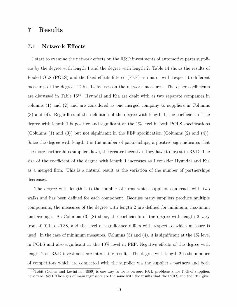
I start to examine the network effects on the R&D investments of automotive parts suppli-

ers by the degree with length 1 and the degree with length 2. Table 14 shows the results of

Pooled OLS (POLS) and the fixed effects filtered (FEF) estimator with respect to different

measures of the degree. Table 14 focuses on the network measures. The other coefficients

are discussed in Table 1615. Hyundai and Kia are dealt with as two separate companies in

columns (1) and (2) and are considered as one merged company to suppliers in Columns

(3) and (4). Regardless of the definition of the degree with length 1, the coefficient of the

degree with length 1 is positive and significant at the 1% level in both POLS specifications

(Columns (1) and (3)) but not significant in the FEF specification (Columns (2) and (4)).

Since the degree with length 1 is the number of partnerships, a positive sign indicates that

the more partnerships suppliers have, the greater incentives they have to invest in R&D. The

size of the coefficient of the degree with length 1 increases as I consider Hyundai and Kia

as a merged firm. This is a natural result as the variation of the number of partnerships

decreases.

The degree with length 2 is the number of firms which suppliers can reach with two

walks and has been defined for each component. Because many suppliers produce multiple

components, the measures of the degree with length 2 are defined for minimum, maximum

and average. As Columns (3)-(8) show, the coefficients of the degree with length 2 vary

from -0.011 to -0.38, and the level of significance differs with respect to which measure is

used. In the case of minimum measures, Columns (3) and (4), it is significant at the 1% level

in POLS and also significant at the 10% level in FEF. Negative effects of the degree with

length 2 on R&D investment are interesting results. The degree with length 2 is the number

of competitors which are connected with the supplier via the supplier’s partners and both

15Tobit (Cohen and Levinthal, 1989) is one way to focus on zero R&D problems since 70% of suppliershave zero R&D. The signs of main regressors are the same with the results that the POLS and the FEF give.

29

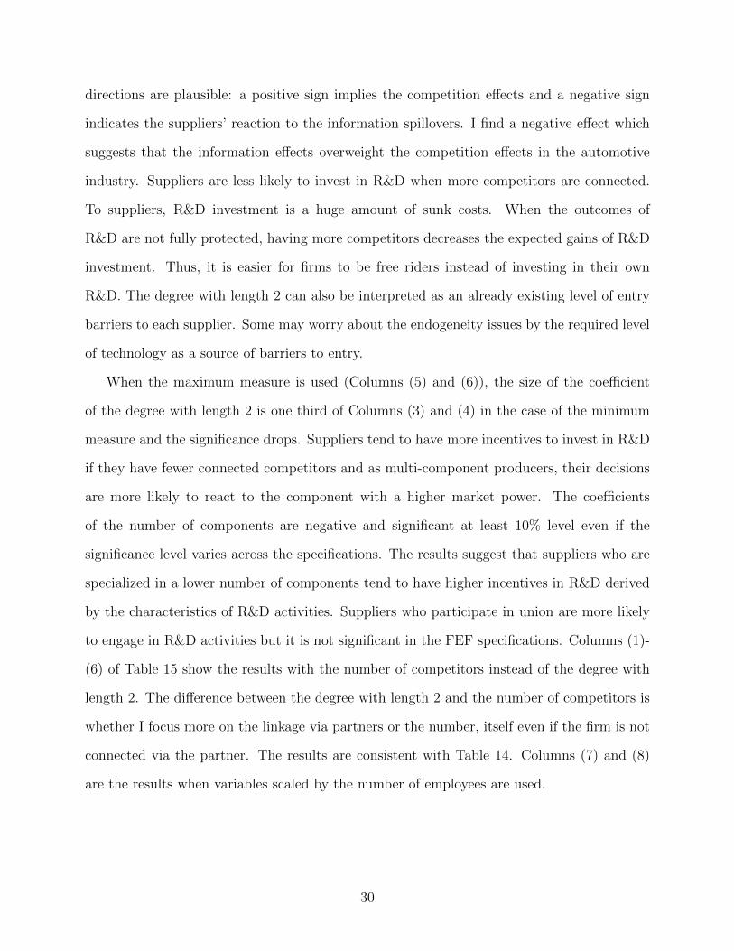
directions are plausible: a positive sign implies the competition effects and a negative sign

indicates the suppliers’ reaction to the information spillovers. I find a negative effect which

suggests that the information effects overweight the competition effects in the automotive

industry. Suppliers are less likely to invest in R&D when more competitors are connected.

To suppliers, R&D investment is a huge amount of sunk costs. When the outcomes of

R&D are not fully protected, having more competitors decreases the expected gains of R&D

investment. Thus, it is easier for firms to be free riders instead of investing in their own

R&D. The degree with length 2 can also be interpreted as an already existing level of entry

barriers to each supplier. Some may worry about the endogeneity issues by the required level

of technology as a source of barriers to entry.

When the maximum measure is used (Columns (5) and (6)), the size of the coefficient

of the degree with length 2 is one third of Columns (3) and (4) in the case of the minimum

measure and the significance drops. Suppliers tend to have more incentives to invest in R&D

if they have fewer connected competitors and as multi-component producers, their decisions

are more likely to react to the component with a higher market power. The coefficients

of the number of components are negative and significant at least 10% level even if the

significance level varies across the specifications. The results suggest that suppliers who are

specialized in a lower number of components tend to have higher incentives in R&D derived

by the characteristics of R&D activities. Suppliers who participate in union are more likely

to engage in R&D activities but it is not significant in the FEF specifications. Columns (1)-

(6) of Table 15 show the results with the number of competitors instead of the degree with

length 2. The difference between the degree with length 2 and the number of competitors is

whether I focus more on the linkage via partners or the number, itself even if the firm is not

connected via the partner. The results are consistent with Table 14. Columns (7) and (8)

are the results when variables scaled by the number of employees are used.

30

7.2 Exclusive Dealing

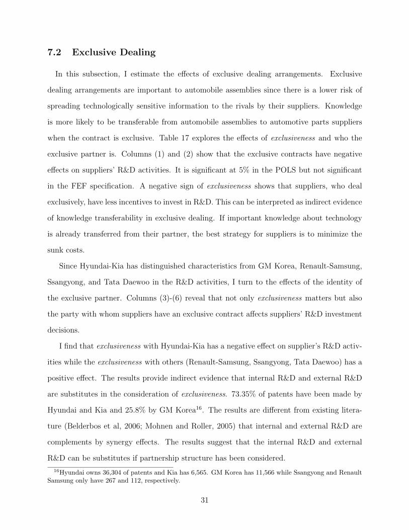
In this subsection, I estimate the effects of exclusive dealing arrangements. Exclusive

dealing arrangements are important to automobile assemblies since there is a lower risk of

spreading technologically sensitive information to the rivals by their suppliers. Knowledge

is more likely to be transferable from automobile assemblies to automotive parts suppliers

when the contract is exclusive. Table 17 explores the effects of exclusiveness and who the

exclusive partner is. Columns (1) and (2) show that the exclusive contracts have negative

effects on suppliers’ R&D activities. It is significant at 5% in the POLS but not significant

in the FEF specification. A negative sign of exclusiveness shows that suppliers, who deal

exclusively, have less incentives to invest in R&D. This can be interpreted as indirect evidence

of knowledge transferability in exclusive dealing. If important knowledge about technology

is already transferred from their partner, the best strategy for suppliers is to minimize the

sunk costs.

Since Hyundai-Kia has distinguished characteristics from GM Korea, Renault-Samsung,

Ssangyong, and Tata Daewoo in the R&D activities, I turn to the effects of the identity of

the exclusive partner. Columns (3)-(6) reveal that not only exclusiveness matters but also

the party with whom suppliers have an exclusive contract affects suppliers’ R&D investment

decisions.

I find that exclusiveness with Hyundai-Kia has a negative effect on supplier’s R&D activ-

ities while the exclusiveness with others (Renault-Samsung, Ssangyong, Tata Daewoo) has a

positive effect. The results provide indirect evidence that internal R&D and external R&D

are substitutes in the consideration of exclusiveness. 73.35% of patents have been made by

Hyundai and Kia and 25.8% by GM Korea16. The results are different from existing litera-

ture (Belderbos et al, 2006; Mohnen and Roller, 2005) that internal and external R&D are

complements by synergy effects. The results suggest that the internal R&D and external

R&D can be substitutes if partnership structure has been considered.

16Hyundai owns 36,304 of patents and Kia has 6,565. GM Korea has 11,566 while Ssangyong and RenaultSamsung only have 267 and 112, respectively.

31

8 Conclusion

In this paper, I focus on the role of supply chain networks in automotive parts suppliers’

R&D decisions in the Korean automobile industry. I examine the hypothesis that stable

supply chain networks are the main source to decrease automotive parts suppliers incentives

to invest in R&D. The stability of the supply chain is based on the long-term relationship

between automotive parts suppliers and automobile assemblies, especially, Hyundai and Kia.

Before testing the hypothesis by panel data techniques, I investigate the importance of net-

works structures in data analysis and test the stability of the supply chain.

First, I present dynamic patterns as evidence that networks structures have to be con-

sidered to interpret the theoretical implications from Sutton’s model. Without the network

structures, patterns of the Korean automobile industry do not explain the insights from Sut-

ton’s endogenous sunk costs model. As market size increased, the number of automotive

parts remained almost the same from 1999 to 2010. However, the automotive parts market

did not seem to be R&D intensive. To explain this contradiction, I focus on information

flows from automobile assemblies to automotive parts suppliers based on the stable supply

chain. Historically, the Korean government encouraged automobile assemblies and automo-

tive parts suppliers to be vertically integrated to maximize the efficiency. As a result, it was

common that the Korean automobile assemblies provided blueprints of parts/components to

their partners based on their long-term partnerships. However, it is not obvious to measure

how knowledge is transferable from automobile assemblies to suppliers in the real world. For

a proxy of the level of knowledge transferability, I use two measures, exclusiveness and the

partnership with Hyundai-Kia and then define four different sectors: Exc-HK, Exc-NonHK,

NonExc-HK and NonExc-NonHK. When networks structures are considered, consistent re-

sults with Sutton’s model are obtainable.

Networks structures are important in the Korean automobile industry because of the sta-

bility of the supply chain. As the second step, I test the stability of supply chain networks

empirically. I consider distance measures based on the graph spectra. I construct the adja-

32

cency matrices for 2008 and 2013. The 2008 adjacency matrix is 806 by 806 since there are

800 suppliers and 6 automobile assemblies. I define the degree matrices and then calculate

the Laplacian matrices and normalize them. The Laplacian matrix is defined as a differ-

ence between the degree matrix and the adjacency matrix. Eigenvalues of the normalized

Laplacian matrices are used to calculate the distance measures such as the Jensen-Shannon

measure. The measures show that the supply chain networks of the Korean automobile in-

dustry are extremely stable over time. This is the first attempt to test the stability of the

networks in Economics.

Based on the importance and stability of the network structures, I estimate the network

effects on automotive parts suppliers’ R&D investments using panel data techniques. I define

various network measures: the degree with length 1, the degree with length 2, exclusiveness,

the number of competitors. The coefficients of network measures are estimated by the Fixed

Effects Filtered estimator. The FEF estimator is applied to estimate both time-variant and

time-invariant regressors, consistently considering the firm-heterogeneity. When correlations

exist between regressors and unobservable firm-heterogeneity, the pooled OLS estimator is

inconsistent and biased. Although the fixed effects estimator is consistent, it cannot estimate

the effects of time-invariant regressors. Since network structures are stable over time, the

network measures are time invariant.

I find that suppliers are more likely to decrease R&D investments as they have more

competitors. The results imply that free-rider effects are greater than competition effects.

The effects of the number of partnerships are not obvious. One of the most interesting results

is that the internal R&D and external R&D are substitutes if the contract is exclusive. When

the suppliers have an exclusive contract with Hyundai-Kia (the biggest R&D investor in

Korea), suppliers have less incentives to invest in R&D. If suppliers had an exclusive contract

with an automobile assemble who has a relatively low level of R&D (Renault-Samsung,

Ssangyong, and Tata Daewoo).

This paper does not contain a direct way to test complementartiy and substitutability.

33

Using the definition by Milgrom and Roberts (1990)17 could be one way to test complemen-

tarity/substitutability. However, applying their methodology directly is difficult because my

data set contains multiple partnerships. The econometrical model I used in this article is

static. At present, Kripfganz and Schwarz (2013) is the only one that has been developed to

estimate time-invariant regressors in the dynamic setting using an the Instrumental variable

method. In addition, the data set contains small sample T problem because T is equal to

12. Although Jackknife methods can be considered, that is beyond the scope of this paper.

17Milgrom and Roberts (1990) defines substitutability by ∂2f∂ri∂rj

< 0 and complementarity by ∂2f∂ri∂rj

> 0.

Athey and Stern (1997) develop a model to test in the discrete setting. If there are two products, x1 and x2,testing the sign of α12 in f(x1, x2) = α0 + α1x1 + α2x2 + α12x1x2.

34

9 Reference

Athey, Susan, and Scott Stern. 1998. “An Empirical Framework for Testing Theories aboutComplementarity in Organizational Design.” National Bureau of Economic Research Work-ing Paper 6600.

Banerjee, Anirban. 2012. “Structural Distance and Evolutionary Relationship of Networks.”Biosystems, 107(3): 186-196.

Berry Steven, and Joel Waldfogel. 2010. “Product Quality and Market Size.” Journal ofIndustrial Economics, 58(1): 1-31.

Belderbos, Rene, Martin Carree, and Boris Lokshin. 2006. “Complementarity in R&DCooperation Strategies.” Review of Industrial Organization, 28: 401-26

Cassiman, Bruno, and Reinhilde Veugelers. 2006, “In Search of Complementarity in Inno-vation Strategy: Internal R&D and External Knowledge Acquisition.” Management Science,52(1): 68-82.

Cohen, W., R. Levin. 1989. Empirical studies of innovation and market structure. R.Schmalensee, R. Willig, eds. Handbook of Industrial Organization. North-Holland, Amster-dam, The Netherlands, 1060-107.

Cohen, Wesley, and Daniel Levinthal. 1989. “Innovation and learning: The two faces ofR&D.” The Economic Journal, 99: 569-596.

Conley, Timothy, and Christopher Udry. 2010. “Learning about a New Technology: Pineap-ple in Ghana.” American Economic Review, 100(1): 35-69

Corchon, Luis, and Simon Wilkie. “Computers, Productivity, and Market Structure.” Work-ing Paper, Instituto Valenciano de Investigationes Economicas.

Ellickson, Paul. 2013. “Supermarkets as a Natural Oligopoly.” Economic Inquiry. 51(2):1142-1154.

Ellickson, Paul. 2007. “Does Sutton apply to supermarkets?.” RAND Journal of Economics.38(1): 43-59.

Foster, Andrew, and Mark Rosenzweig, 1995. “Learning by doing and learning from others:Human capital and technical change in agriculture.” Journal of Political Economy, 103(6):1176-1209.

Fox, Jeremy. 2010. “Estimating Matching Games with Transfers. Working Paper: Uni-versity of Chicago.

35

Gavazza, Alessandro. 2011. “Demand Spillovers and Market Outcomes in the Mutual FundIndustry.” RAND Journal of Economics. 42(4): 776-804.

Grossman, Gene, and Elhanan Helpman. 1991. Innovation and Growth in the Global Econ-omy. Cambridge, MA: MIT Press.

Gereffi, Gary. 2001. “Beyond the Producer-Driven/Buyer-Driver Dichotomy: The Evolu-tion of Global Value Chains in the Internet Era.” IDS Bulletin, 32(3): 30-40.

Hatfield, John, and Fuhito Kojima. 2008. “Matching with Contracts: Comment.” AmericanEconomic Review, 98(3): 1189-94.

Hatfield, John, and Scott Kominers. 2012. “Matching in Networks with Bilateral Con-tracts.” American Economic Journal: Microeconomics 4(1): 174-208.

Hsiao, Cheng. 2003. Analysis of Panel Data. Cambridge University Press.

Jackson, Matthew. 2008. Social and Economic Networks. Princeton University Press.

Jurman, Giuseppe, Roberto Visintaniner, and Cesare Furlanello. 2011. “An Introductionto Spectral Distances in Networks.” Neural Nets WIRN10: Proceedings of the 20th ItalianWorkshop on Neural Nets, 227-34. IOS Press Amsterdam.

Jo, Hyung Je and Joo Eun Cho. 2012. “Does Hyundai Motor Company’s ProductionManagement Converge to ”Pull’ Production?: A Study of the Evolution of Demand-drivenProduction Management through Information System.” Korean Journal of Sociology, 46(5):233-57.

Kenny, Martin, and Richard Florida. 1994. “Japanese Maquiladoras: Production Orga-nization and Global Commodity Chains.” World Development 22: 27-44.

Kim, Se-jik, and Hyun Song Shin. 2012. “Sustaining Production Chains Through FinancialLinkages.” American Economic Review, 102(3): 402-406.

Lee, Hangkoo. 2011. “Advantages of Vertical Integrations in the Automobile Industry.”KAIBM & KASME Conference, 309-25

Lin, Jianhua. 1991. ”Divergence Measures Based on the Shannon Entropy,” IEEE Transac-tions on Information Theory, 37(1): 145-51.

Milgrom, Paul, and John Roberts. 1990. “The Economics of Modern Manufacturing: Tech-nology, Strategy, and Organization.” American Economic Review, 80(3): 511-528

Munshi, Laivan, and Jacques Myaux. 2006. “Social Norms and the Fertility Transition.”Journal of Development Economics, 80: 1-38

36

Munshi, Laivan. 2004. “Social Learning in a Heterogeneous Population: Technology Diffu-sion in the Indian Green Revolution.” Journal of Development Economics, 73: 183-213

Ostrovsky, Michael. 2008. “Stability in Supply Chain Networks.” American Economic Re-view, 98(3): 897-923.

Park, Minjung. 2013. “Advertising and Market Share Dynamics.” Working Paper.

Pesaran, Hashem, and Qiankun Zhou. 2014. “Estimation of Time-invariant Effects in StaticPanel Data Models.” Center for Applied Financial Economics Research Paper, University ofSouthern California.

Pincombe, Brandon. 2007. ”Detecting Changes in Time Series of Network Graphs usingMinimum Mean Squared Error and Cumulative Summation.” ANZIAM Journal 48: 450-73.

Sutton, John. 1991. Sunk Costs and Market Structure: Price Competition, Advertising,and the Evolution of Concentration (MIT Press).

Sutton, John. 2007. Market Structure: Theory and Evidence. Handbook of IndustrialOrganization.

37

38

Figure 1. Four segments with respect to exclusiveness and partnerships

Table 1: Policy changes in South Korea from 1962 to 2012

Period Title Characteristics

I 1962-1971 Localization Domestic market protection and nurturing auto makers

II 1972-1976 Quantitative growth Developing native model and producton capability

III 1977-1981 Mass production Large-scale production and export strategies

IV 1982-1991 Liberalization Decreasing the tariff from 50% to 20%

V 1992-1997 Technology

innovation Capacity expansion and self-reliance of technology

VI 1998-2002 Qualitative growth Promoting globalization and innovation , attracting foreign direct investment

VII 2003-2007 Regulation Regulations of environment and safety and future oriented vehicle development plan

VIII 2008-2012 Green car project Developing new engines to growth

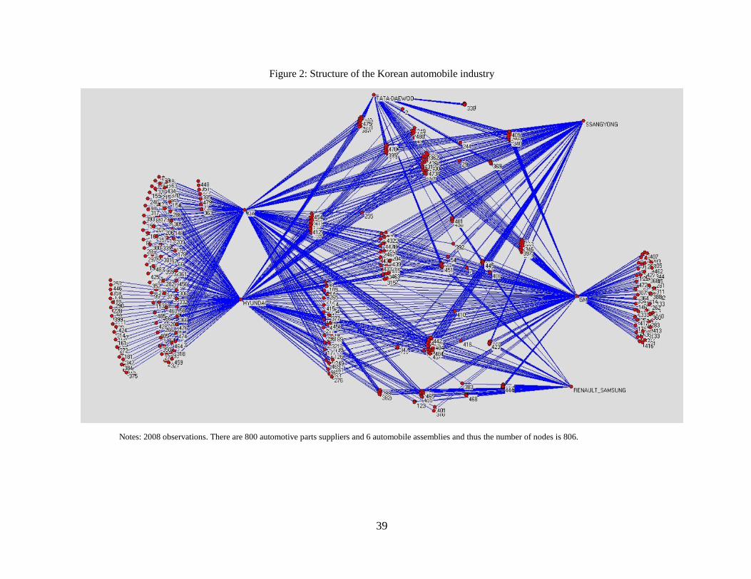
39

Figure 2: Structure of the Korean automobile industry

Notes: 2008 observations. There are 800 automotive parts suppliers and 6 automobile assemblies and thus the number of nodes is 806.

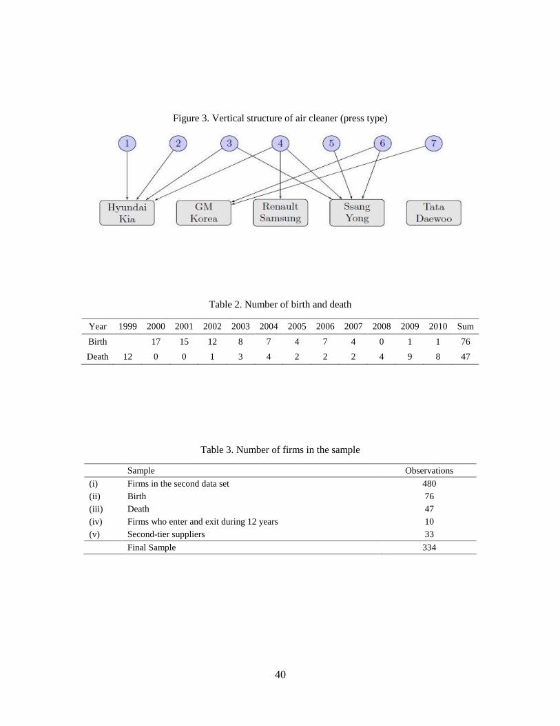
40

Figure 3. Vertical structure of air cleaner (press type)

Table 2. Number of birth and death

Year 1999 2000 2001 2002 2003 2004 2005 2006 2007 2008 2009 2010 Sum

Birth 17 15 12 8 7 4 7 4 0 1 1 76

Death 12 0 0 1 3 4 2 2 2 4 9 8 47

Table 3. Number of firms in the sample

Sample Observations

(i) Firms in the second data set 480

(ii) Birth 76

(iii) Death 47

(iv) Firms who enter and exit during 12 years 10

(v) Second-tier suppliers 33

Final Sample 334

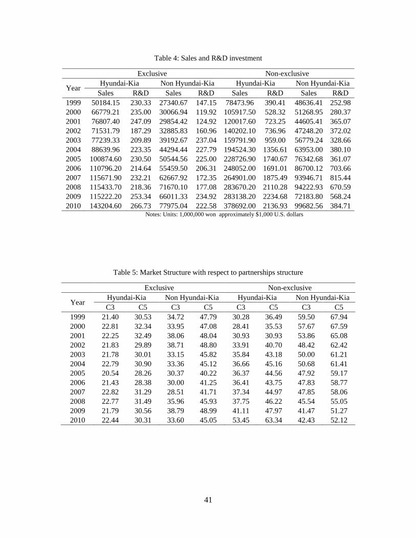
41

Table 4: Sales and R&D investment

Exclusive Non-exclusive

Year Hyundai-Kia Non Hyundai-Kia Hyundai-Kia Non Hyundai-Kia

Sales R&D Sales R&D Sales R&D Sales R&D

1999 50184.15 230.33 27340.67 147.15 78473.96 390.41 48636.41 252.98

2000 66779.21 235.00 30066.94 119.92 105917.50 528.32 51268.95 280.37

2001 76807.40 247.09 29854.42 124.92 120017.60 723.25 44605.41 365.07

2002 71531.79 187.29 32885.83 160.96 140202.10 736.96 47248.20 372.02

2003 77239.33 209.89 39192.67 237.04 159791.90 959.00 56779.24 328.66

2004 88639.96 223.35 44294.44 227.79 194524.30 1356.61 63953.00 380.10

2005 100874.60 230.50 50544.56 225.00 228726.90 1740.67 76342.68 361.07

2006 110796.20 214.64 55459.50 206.31 248052.00 1691.01 86700.12 703.66

2007 115671.90 232.21 62667.92 172.35 264901.00 1875.49 93946.71 815.44

2008 115433.70 218.36 71670.10 177.08 283670.20 2110.28 94222.93 670.59

2009 115222.20 253.34 66011.33 234.92 283138.20 2234.68 72183.80 568.24

2010 143204.60 266.73 77975.04 222.58 378692.00 2136.93 99682.56 384.71 Notes: Units: 1,000,000 won approximately $1,000 U.S. dollars

Table 5: Market Structure with respect to partnerships structure

Exclusive Non-exclusive

Year Hyundai-Kia Non Hyundai-Kia Hyundai-Kia Non Hyundai-Kia

C3 C5 C3 C5 C3 C5 C3 C5

1999 21.40 30.53 34.72 47.79 30.28 36.49 59.50 67.94

2000 22.81 32.34 33.95 47.08 28.41 35.53 57.67 67.59

2001 22.25 32.49 38.06 48.04 30.93 30.93 53.86 65.08

2002 21.83 29.89 38.71 48.80 33.91 40.70 48.42 62.42

2003 21.78 30.01 33.15 45.82 35.84 43.18 50.00 61.21

2004 22.79 30.90 33.36 45.12 36.66 45.16 50.68 61.41

2005 20.54 28.26 30.37 40.22 36.37 44.56 47.92 59.17

2006 21.43 28.38 30.00 41.25 36.41 43.75 47.83 58.77

2007 22.82 31.29 28.51 41.71 37.34 44.97 47.85 58.06

2008 22.77 31.49 35.96 45.93 37.75 46.22 45.54 55.05

2009 21.79 30.56 38.79 48.99 41.11 47.97 41.47 51.27

2010 22.44 30.31 33.60 45.05 53.45 63.34 42.43 52.12

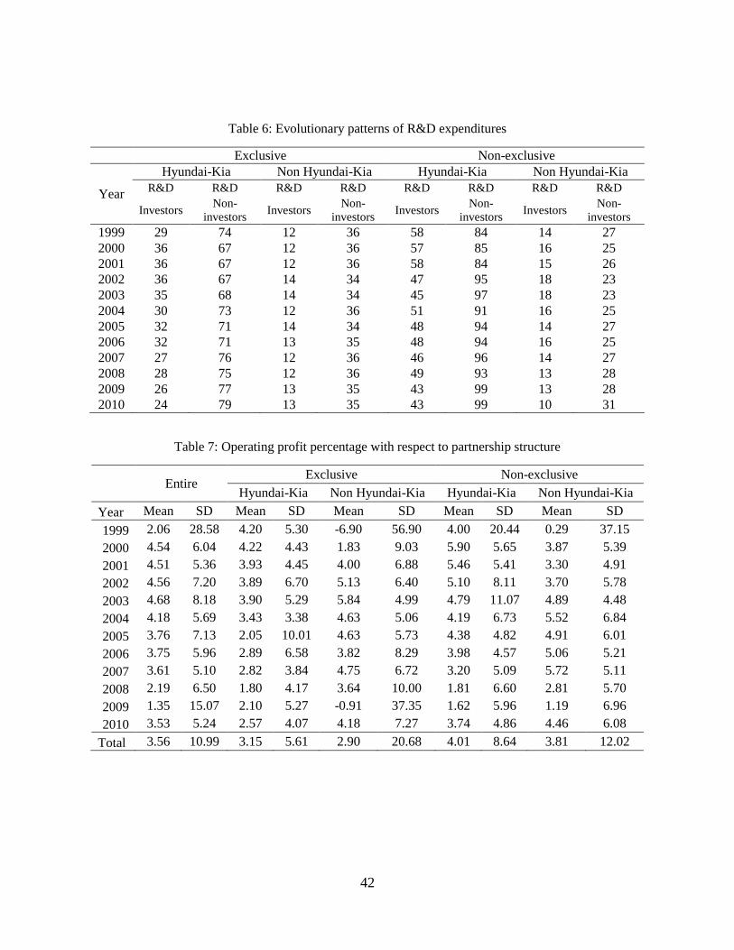
42

Table 6: Evolutionary patterns of R&D expenditures

Exclusive Non-exclusive

Year

Hyundai-Kia Non Hyundai-Kia Hyundai-Kia Non Hyundai-Kia

R&D R&D R&D R&D R&D R&D R&D R&D

Investors Non-

investors Investors

Non-

investors Investors

Non-

investors Investors

Non-

investors

1999 29 74 12 36 58 84 14 27

2000 36 67 12 36 57 85 16 25

2001 36 67 12 36 58 84 15 26

2002 36 67 14 34 47 95 18 23

2003 35 68 14 34 45 97 18 23

2004 30 73 12 36 51 91 16 25

2005 32 71 14 34 48 94 14 27

2006 32 71 13 35 48 94 16 25

2007 27 76 12 36 46 96 14 27

2008 28 75 12 36 49 93 13 28

2009 26 77 13 35 43 99 13 28

2010 24 79 13 35 43 99 10 31

Table 7: Operating profit percentage with respect to partnership structure

Entire

Exclusive Non-exclusive

Hyundai-Kia Non Hyundai-Kia Hyundai-Kia Non Hyundai-Kia

Year Mean SD Mean SD Mean SD Mean SD Mean SD

1999 2.06 28.58 4.20 5.30 -6.90 56.90 4.00 20.44 0.29 37.15

2000 4.54 6.04 4.22 4.43 1.83 9.03 5.90 5.65 3.87 5.39

2001 4.51 5.36 3.93 4.45 4.00 6.88 5.46 5.41 3.30 4.91

2002 4.56 7.20 3.89 6.70 5.13 6.40 5.10 8.11 3.70 5.78

2003 4.68 8.18 3.90 5.29 5.84 4.99 4.79 11.07 4.89 4.48

2004 4.18 5.69 3.43 3.38 4.63 5.06 4.19 6.73 5.52 6.84

2005 3.76 7.13 2.05 10.01 4.63 5.73 4.38 4.82 4.91 6.01

2006 3.75 5.96 2.89 6.58 3.82 8.29 3.98 4.57 5.06 5.21

2007 3.61 5.10 2.82 3.84 4.75 6.72 3.20 5.09 5.72 5.11

2008 2.19 6.50 1.80 4.17 3.64 10.00 1.81 6.60 2.81 5.70

2009 1.35 15.07 2.10 5.27 -0.91 37.35 1.62 5.96 1.19 6.96

2010 3.53 5.24 2.57 4.07 4.18 7.27 3.74 4.86 4.46 6.08

Total 3.56 10.99 3.15 5.61 2.90 20.68 4.01 8.64 3.81 12.02

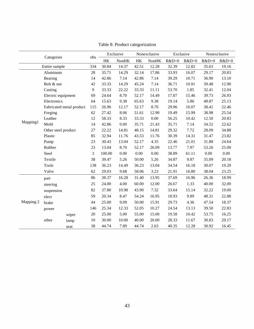
43

Table 8: Product categorization

Categories obs Exclusive Nonexclusive Exclusive Nonexclusive

HK NonHK HK NonHK R&D=0 R&D>0 R&D=0 R&D>0

Entire sample 334 30.84 14.37 42.51 12.28 32.39 12.82 35.63 19.16

Mapping1

Aluminum 28 35.71 14.29 32.14 17.86 33.93 16.07 29.17 20.83

Bearing 14 42.86 7.14 42.86 7.14 39.29 10.71 36.90 13.10

Bolt & nut 42 33.33 14.29 45.24 7.14 36.71 10.91 39.48 12.90

Casting 9 33.33 22.22 33.33 11.11 53.70 1.85 32.41 12.04

Electric equipment 69 24.64 8.70 52.17 14.49 17.87 15.46 39.73 26.93

Electronics 64 15.63 9.38 65.63 9.38 19.14 5.86 49.87 25.13

Fabricated metal product 115 26.96 12.17 52.17 8.70 29.06 10.07 38.41 22.46

Forging 62 27.42 8.06 51.61 12.90 19.49 15.99 38.98 25.54

Leather 12 58.33 8.33 33.33 0.00 56.25 10.42 12.50 20.83

Mold 14 42.86 0.00 35.71 21.43 35.71 7.14 34.52 22.62

Other steel product 27 22.22 14.81 48.15 14.81 29.32 7.72 28.09 34.88

Plastic 85 32.94 11.76 43.53 11.76 30.39 14.31 31.47 23.82

Pump 23 30.43 13.04 52.17 4.35 22.46 21.01 31.88 24.64

Rubber 23 13.04 8.70 52.17 26.09 13.77 7.97 53.26 25.00

Steel 3 100.00 0.00 0.00 0.00 38.89 61.11 0.00 0.00

Textile 38 39.47 5.26 50.00 5.26 34.87 9.87 35.09 20.18

Tools 138 36.23 14.49 36.23 13.04 34.54 16.18 30.07 19.20

Valve 62 29.03 9.68 58.06 3.23 21.91 16.80 38.04 23.25

Mapping 2

part 86 38.37 16.28 31.40 13.95 37.69 16.96 26.36 18.99

steering 25 24.00 4.00 60.00 12.00 26.67 1.33 40.00 32.00

suspension 82 37.80 10.98 43.90 7.32 33.64 15.14 32.22 19.00

elect 59 20.34 8.47 54.24 16.95 18.93 9.89 48.31 22.88

brake 44 25.00 9.09 50.00 15.91 29.73 4.36 47.54 18.37

power 146 25.34 12.33 52.05 10.27 24.54 13.13 39.50 22.83

other

wiper 20 25.00 5.00 55.00 15.00 19.58 10.42 53.75 16.25

lamp 10 30.00 10.00 40.00 20.00 28.33 11.67 30.83 29.17

seat 38 44.74 7.89 44.74 2.63 40.35 12.28 30.92 16.45

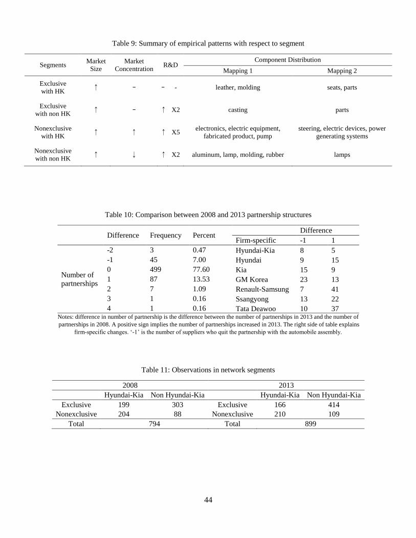
44

Table 9: Summary of empirical patterns with respect to segment

Segments Market

Size

Market

Concentration R&D

Component Distribution

Mapping 1 Mapping 2

Exclusive

with HK ↑ - - - leather, molding seats, parts

Exclusive

with non HK ↑ - ↑ X2 casting parts

Nonexclusive

with HK ↑ ↑ ↑ X5

electronics, electric equipment,

fabricated product, pump

steering, electric devices, power

generating systems

Nonexclusive

with non HK ↑ ↓ ↑ X2 aluminum, lamp, molding, rubber lamps

Table 10: Comparison between 2008 and 2013 partnership structures

Difference Frequency Percent

Difference

Firm-specific -1 1

Number of

partnerships

-2 3 0.47 Hyundai-Kia 8 5

-1 45 7.00 Hyundai 9 15

0 499 77.60 Kia 15 9

1 87 13.53 GM Korea 23 13

2 7 1.09 Renault-Samsung 7 41

3 1 0.16 Ssangyong 13 22

4 1 0.16 Tata Deawoo 10 37 Notes: difference in number of partnership is the difference between the number of partnerships in 2013 and the number of

partnerships in 2008. A positive sign implies the number of partnerships increased in 2013. The right side of table explains

firm-specific changes. ‘-1’ is the number of suppliers who quit the partnership with the automobile assembly.

Table 11: Observations in network segments

2008 2013

Hyundai-Kia Non Hyundai-Kia Hyundai-Kia Non Hyundai-Kia

Exclusive 199 303 Exclusive 166 414

Nonexclusive 204 88 Nonexclusive 210 109

Total 794 Total 899

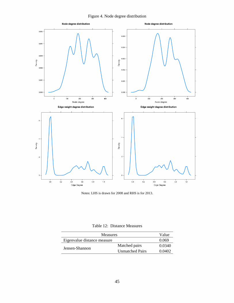
45

Figure 4. Node degree distribution

Notes: LHS is drawn for 2008 and RHS is for 2013.

Table 12: Distance Measures

Measures Value

Eigenvalue distance measure 0.069

Jensen-Shannon Matched pairs 0.0340

Unmatched Pairs 0.0402

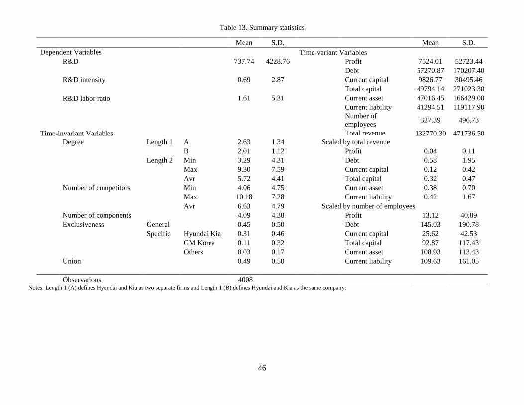
46

Table 13. Summary statistics

Mean S.D. Mean S.D.

Dependent Variables Time-variant Variables

R&D 737.74 4228.76 Profit 7524.01 52723.44

Debt 57270.87 170207.40

R&D intensity 0.69 2.87 Current capital 9826.77 30495.46

Total capital 49794.14 271023.30

R&D labor ratio 1.61 5.31 Current asset 47016.45 166429.00

Current liability 41294.51 119117.90

Number of

employees 327.39 496.73

Time-invariant Variables Total revenue 132770.30 471736.50

Degree Length 1 A 2.63 1.34 Scaled by total revenue

B 2.01 1.12 Profit 0.04 0.11

Length 2 Min 3.29 4.31 Debt 0.58 1.95

Max 9.30 7.59 Current capital 0.12 0.42

Avr 5.72 4.41 Total capital 0.32 0.47

Number of competitors Min 4.06 4.75 Current asset 0.38 0.70

Max 10.18 7.28 Current liability 0.42 1.67

Avr 6.63 4.79 Scaled by number of employees

Number of components 4.09 4.38 Profit 13.12 40.89

Exclusiveness General 0.45 0.50 Debt 145.03 190.78

Specific Hyundai Kia 0.31 0.46 Current capital 25.62 42.53

GM Korea 0.11 0.32 Total capital 92.87 117.43

Others 0.03 0.17 Current asset 108.93 113.43

Union 0.49 0.50 Current liability 109.63 161.05

Observations 4008 Notes: Length 1 (A) defines Hyundai and Kia as two separate firms and Length 1 (B) defines Hyundai and Kia as the same company.

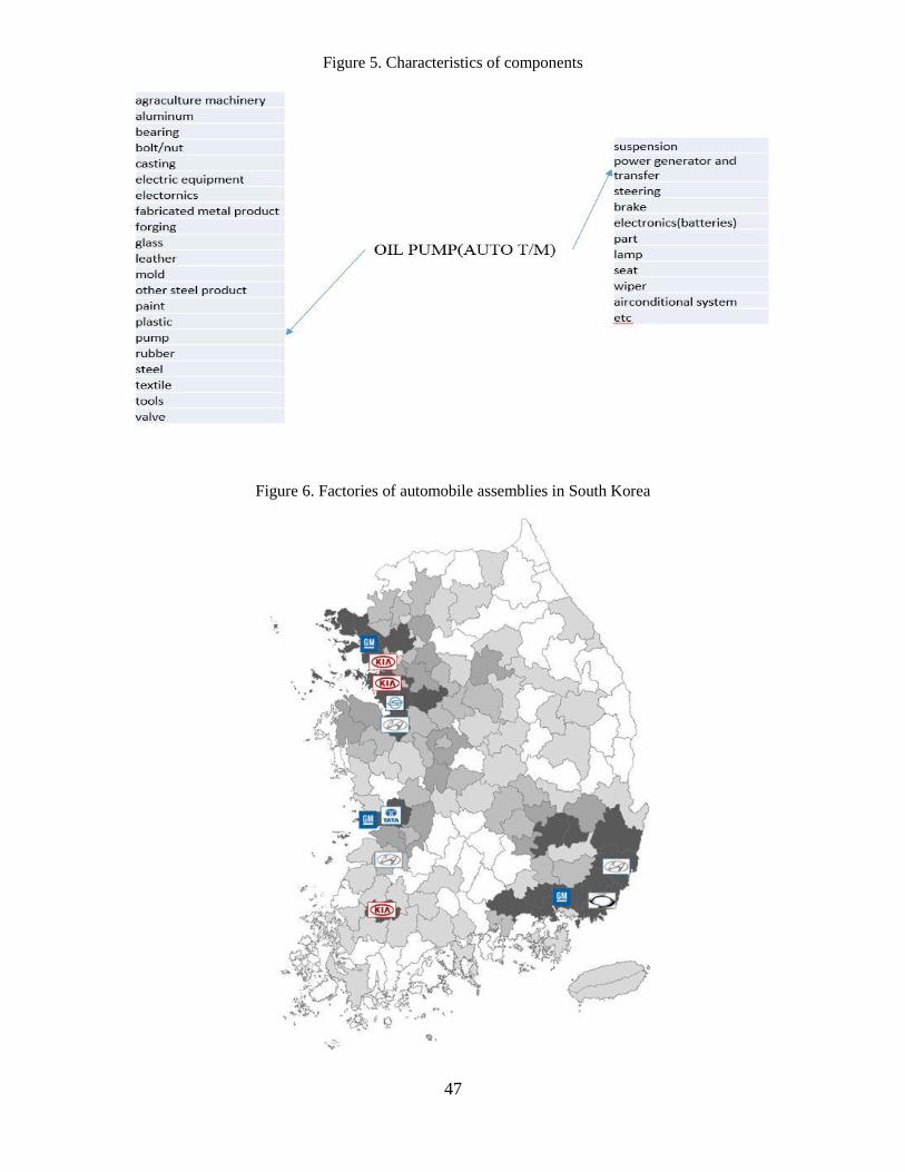
47

Figure 5. Characteristics of components

Figure 6. Factories of automobile assemblies in South Korea

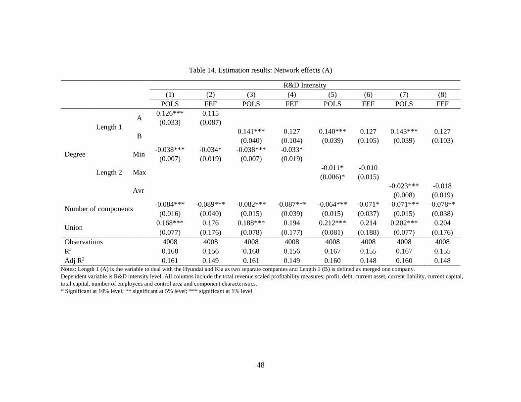
48

Table 14. Estimation results: Network effects (A)

R&D Intensity

(1) (2) (3) (4) (5) (6) (7) (8)

POLS FEF POLS FEF POLS FEF POLS FEF

Degree

Length 1

A 0.126*** 0.115

(0.033) (0.087)

B 0.141*** 0.127 0.140*** 0.127 0.143*** 0.127

(0.040) (0.104) (0.039) (0.105) (0.039) (0.103)

Length 2

Min -0.038*** -0.034* -0.038*** -0.033*

(0.007) (0.019) (0.007) (0.019)

Max -0.011* -0.010

(0.006)* (0.015)

Avr -0.023*** -0.018

(0.008) (0.019)

Number of components -0.084*** -0.089*** -0.082*** -0.087*** -0.064*** -0.071* -0.071*** -0.078**

(0.016) (0.040) (0.015) (0.039) (0.015) (0.037) (0.015) (0.038)

Union 0.168*** 0.176 0.188*** 0.194 0.212*** 0.214 0.202*** 0.204

(0.077) (0.176) (0.078) (0.177) (0.081) (0.188) (0.077) (0.176)

Observations 4008 4008 4008 4008 4008 4008 4008 4008

R2 0.168 0.156 0.168 0.156 0.167 0.155 0.167 0.155

Adj R2 0.161 0.149 0.161 0.149 0.160 0.148 0.160 0.148 Notes: Length 1 (A) is the variable to deal with the Hyundai and Kia as two separate companies and Length 1 (B) is defined as merged one company.

Dependent variable is R&D intensity level. All columns include the total revenue scaled profitability measures; profit, debt, current asset, current liability, current capital,

total capital, number of employees and control area and component characteristics.

* Significant at 10% level; ** significant at 5% level; *** significant at 1% level

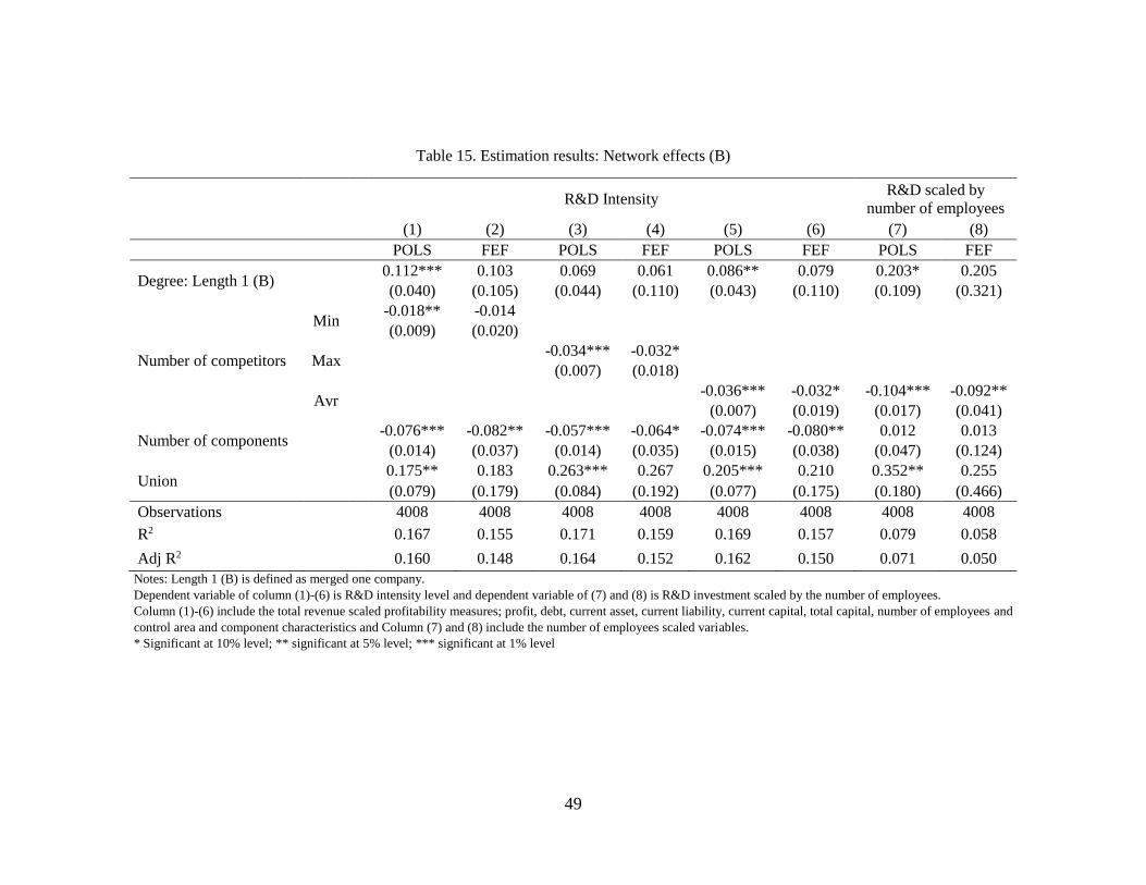
49

Table 15. Estimation results: Network effects (B)

R&D Intensity

R&D scaled by

number of employees

(1) (2) (3) (4) (5) (6) (7) (8)

POLS FEF POLS FEF POLS FEF POLS FEF

Degree: Length 1 (B) 0.112*** 0.103 0.069 0.061 0.086** 0.079 0.203* 0.205

(0.040) (0.105) (0.044) (0.110) (0.043) (0.110) (0.109) (0.321)

Number of competitors

Min -0.018** -0.014

(0.009) (0.020)

Max -0.034*** -0.032*

(0.007) (0.018)

Avr -0.036*** -0.032* -0.104*** -0.092**

(0.007) (0.019) (0.017) (0.041)

Number of components -0.076*** -0.082** -0.057*** -0.064* -0.074*** -0.080** 0.012 0.013

(0.014) (0.037) (0.014) (0.035) (0.015) (0.038) (0.047) (0.124)

Union 0.175** 0.183 0.263*** 0.267 0.205*** 0.210 0.352** 0.255

(0.079) (0.179) (0.084) (0.192) (0.077) (0.175) (0.180) (0.466)

Observations 4008 4008 4008 4008 4008 4008 4008 4008

R2 0.167 0.155 0.171 0.159 0.169 0.157 0.079 0.058

Adj R2 0.160 0.148 0.164 0.152 0.162 0.150 0.071 0.050

Notes: Length 1 (B) is defined as merged one company.

Dependent variable of column (1)-(6) is R&D intensity level and dependent variable of (7) and (8) is R&D investment scaled by the number of employees.

Column (1)-(6) include the total revenue scaled profitability measures; profit, debt, current asset, current liability, current capital, total capital, number of employees and

control area and component characteristics and Column (7) and (8) include the number of employees scaled variables.

* Significant at 10% level; ** significant at 5% level; *** significant at 1% level

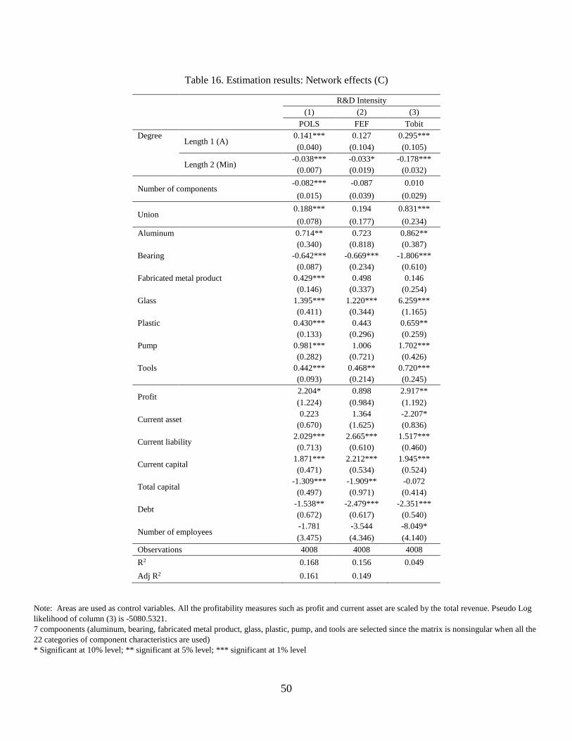
50

Table 16. Estimation results: Network effects (C)

R&D Intensity

(1) (2) (3)

POLS FEF Tobit

Degree Length 1 (A)

0.141*** 0.127 0.295***

(0.040) (0.104) (0.105)

Length 2 (Min)

-0.038*** -0.033* -0.178***

(0.007) (0.019) (0.032)

Number of components -0.082*** -0.087 0.010

(0.015) (0.039) (0.029)

Union 0.188*** 0.194 0.831***

(0.078) (0.177) (0.234)

Aluminum 0.714** 0.723 0.862**

(0.340) (0.818) (0.387)

Bearing -0.642*** -0.669*** -1.806***

(0.087) (0.234) (0.610)

Fabricated metal product 0.429*** 0.498 0.146

(0.146) (0.337) (0.254)

Glass 1.395*** 1.220*** 6.259***

(0.411) (0.344) (1.165)

Plastic 0.430*** 0.443 0.659**

(0.133) (0.296) (0.259)

Pump 0.981*** 1.006 1.702***

(0.282) (0.721) (0.426)

Tools 0.442*** 0.468** 0.720***

(0.093) (0.214) (0.245)

Profit 2.204* 0.898 2.917**

(1.224) (0.984) (1.192)

Current asset 0.223 1.364 -2.207*

(0.670) (1.625) (0.836)

Current liability 2.029*** 2.665*** 1.517***

(0.713) (0.610) (0.460)

Current capital 1.871*** 2.212*** 1.945***

(0.471) (0.534) (0.524)

Total capital -1.309*** -1.909** -0.072

(0.497) (0.971) (0.414)

Debt -1.538** -2.479*** -2.351***

(0.672) (0.617) (0.540)

Number of employees -1.781 -3.544 -8.049*

(3.475) (4.346) (4.140)

Observations 4008 4008 4008

R2 0.168 0.156 0.049

Adj R2 0.161 0.149

Note: Areas are used as control variables. All the profitability measures such as profit and current asset are scaled by the total revenue. Pseudo Log

likelihood of column (3) is -5080.5321.

7 compoonents (aluminum, bearing, fabricated metal product, glass, plastic, pump, and tools are selected since the matrix is nonsingular when all the

22 categories of component characteristics are used)

* Significant at 10% level; ** significant at 5% level; *** significant at 1% level

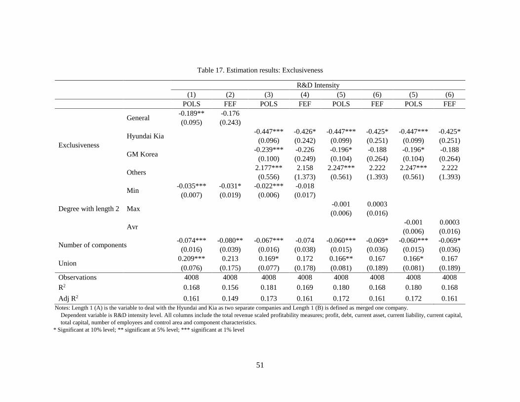
51

Table 17. Estimation results: Exclusiveness

R&D Intensity

(1) (2) (3) (4) (5) (6) (5) (6)

POLS FEF POLS FEF POLS FEF POLS FEF

Exclusiveness

General -0.189** -0.176

(0.095) (0.243)

Hyundai Kia -0.447*** -0.426* -0.447*** -0.425* -0.447*** -0.425*

(0.096) (0.242) (0.099) (0.251) (0.099) (0.251)

GM Korea -0.239*** -0.226 -0.196* -0.188 -0.196* -0.188

(0.100) (0.249) (0.104) (0.264) (0.104) (0.264)

Others 2.177*** 2.158 2.247*** 2.222 2.247*** 2.222

(0.556) (1.373) (0.561) (1.393) (0.561) (1.393)

Degree with length 2

Min -0.035*** -0.031* -0.022*** -0.018

(0.007) (0.019) (0.006) (0.017)

Max -0.001 0.0003

(0.006) (0.016)

Avr -0.001 0.0003

(0.006) (0.016)

Number of components -0.074*** -0.080** -0.067*** -0.074 -0.060*** -0.069* -0.060*** -0.069*

(0.016) (0.039) (0.016) (0.038) (0.015) (0.036) (0.015) (0.036)

Union 0.209*** 0.213 0.169* 0.172 0.166** 0.167 0.166* 0.167

(0.076) (0.175) (0.077) (0.178) (0.081) (0.189) (0.081) (0.189)

Observations 4008 4008 4008 4008 4008 4008 4008 4008

R2 0.168 0.156 0.181 0.169 0.180 0.168 0.180 0.168

Adj R2 0.161 0.149 0.173 0.161 0.172 0.161 0.172 0.161

Notes: Length 1 (A) is the variable to deal with the Hyundai and Kia as two separate companies and Length 1 (B) is defined as merged one company.

Dependent variable is R&D intensity level. All columns include the total revenue scaled profitability measures; profit, debt, current asset, current liability, current capital,

total capital, number of employees and control area and component characteristics.

* Significant at 10% level; ** significant at 5% level; *** significant at 1% level