1  

 

 

 

 

 

 

 

 

 

When Demand Increases Cause Shakeouts 

Thomas N. Hubbard* 

Michael J. Mazzeo** 

DRAFT – July 19, 2017 

 

 

Standard economic models  that guide competition policy  imply  that demand  increases should  lead  to 

more,  not  fewer  firms.    However,  Sutton’s  (1991)  model  illustrates  that  in  some  cases,  demand 

increases can catalyze competitive responses that bring about shake‐outs.  This paper provides empirical 

evidence  of  this  effect  in  the  1960s‐1980s  hotel  and  motel  industry,  an  industry  where  quality 

competition  increasingly took the form of whether firms supplied outdoor recreational amenities such 

as swimming pools.  We find that openings of new Interstate Highways are associated with increases in 

hotel employment, but decreases  in  the number of  firms,  in  local areas.   We  further  find  that while 

highway construction is associated with increases in hotel employment in both warm and cold places, it 

only  leads to fewer firms  in warm places (where outdoor amenities were more valued by consumers).  

Finally, we  find  no  evidence  of  this  effect  in  other  industries  that  serve  highway  travelers,  gasoline 

retailing or restaurants, where quality competition  is either  less  important or quality  is supplied more 

through variable  costs.   We discuss  the  implications of  these  results  for  competition policy, and how 

they highlight  the  importance and  challenge of distinguishing between “natural” and “market‐power‐

driven” increases in concentration.  

 

*Kellogg School of Management, Northwestern University and NBER. 

**Kellogg School of Management, Northwestern University.   

2  

I. Introduction 

Shake‐outs,  episodes  where  the  number  of  firms  in  an  industry  significantly  decreases,  are  a 

common industry dynamic.  While their details differ – some may be due simply to the exit of incumbent 

firms, while  others may  be  due  to  a  series  of  horizontal mergers  –  all  lead  to  increases  in market 

concentration.    A  long  tradition  in  industrial  organization  and  antitrust  law  associates  increases  in 

concentration  with  decreases  in  competition.    Thus,  what  drives  shake‐outs  is  a  key  question  in 

competition policy and its application to particular industries.   In many standard models of competition, 

increases in demand (weakly) lead to more firms and thus decreases in concentration, and decreases in 

demand  lead  (weakly)  to  fewer  firms  and  thus  increases  in  concentration.    These  standard models 

suggest  a  potential  screen  for whether  shake‐outs  are  due  to  competitive  factors,  or  reflect  firms’ 

attempts  to obtain or  increase market power:  shake‐outs due  to demand decreases are  likely due  to 

competitive factors, but shake‐outs that are associated with demand  increases should be viewed with 

suspicion,  since  standard  models  do  not  imply  that  demand  increases  should  lead  to  shake‐outs.   

Increases in concentration across industries where demand is almost certainly increasing have led policy 

makers  in the United States and the European Union to become concerned that “competition may be 

decreasing  in many  economic  sectors”  and  that  consumers  would  benefit  from  a more  aggressive 

competition policy.1 

Important  theoretical  contributions by Shaked and  Sutton  (1987) and Sutton  (1991) highlight  the 

difficulty of utilizing simple rules of thumb for distinguishing between cases where shake‐outs are due to 

“natural” competitive factors or firms’ success in obtaining or increasing their market power, however.   

These models show that in industries where competition is in quality, and quality is produced with fixed 

costs,  increases  in demand can catalyze a competitive response that brings about shake‐outs – higher 

demand  can  lead  to  fewer  firms.    Shake‐outs  can  be  due  to  competitive  factors,  and  in  fact  can  be 

initiated by  increases  in demand, even  in  industries where there are no new technologies that provide 

firms scale‐related advantages. 

This paper provides empirical evidence of this effect in the context of hotels and motels in the mid‐

to‐late 20th  century, where  the  completion of  interstate highways across  the United States  increased 

demand in different non‐urban areas at different times, and where an increasingly important element of 

quality competition took the form of whether firms supplied recreational amenities such as swimming 

pools.  We first provide evidence that the completion of Interstate highways is associated greater local 

                                                            1 “Benefits of Competition and Indicators of Market Power,” Council of Economic Advisers Issue Brief, April 2016.  

3  

demand for lodging, showing that it is associated with increases in hotel/motel employment.  We then 

investigate how local industry structure adjusts to these shocks; we show that highway completion leads 

to fewer (but larger) hotels and motels.   On average in our sample counties, the completion of highways 

leads to shakeouts.   

We then provide evidence on whether the shake‐outs in our sample are due to quality competition 

by  examining  whether  this  effect  is  stronger  in  warmer  areas  where  the  returns  to  investment  in 

outdoor recreational amenities (i.e., swimming pools) are greater.   We show that while the  increase  in 

employment in this industry is the same in warmer and cooler regions, highway completion only led to 

shakeouts in warmer regions.  Finally, we provide further evidence on quality competition and changes 

in market  structure  by  adopting  a  strategy  similar  to  Berry  and Waldfogel  (2010).   We  investigate 

whether these effects appear also when looking at gas retailing or restaurants, industries where quality 

competition  is either  less  important or quality  is supplied primarily  through variable costs rather  than 

fixed costs.   Unlike  for hotels and motels, we  find no evidence  that highway completion  is associated 

with shakeouts in these industries. 

Our evidence connects to an important finding of Sutton (1991) that to our knowledge has not been 

investigated by the previous empirical literature: shakeouts – which in some cases could take the form 

or mergers or merger waves – can be catalyzed by increases in market size.  The competitive responses 

that lead to shake‐outs need not only be initiated by changes in the “technology” that produces quality 

(for example, in the case of consumer packaged goods, national television advertising in the 1950s and 

1960s), but sometimes can be initiated simply by positive demand shocks.   Firms’ incentives to grow – 

and in some cases to merge with other firms ‐‐ in response to demand increases need not be motivated 

by anticompetitive  incentives, but  rather may be motivated by  increased  incentives  to compete more 

effectively on nonprice dimensions.   Distinguishing between mergers that reflect changes  in how firms 

compete,  but  not  necessarily  decreases  in  competition,  and  mergers  that  lead  to  decreases  in 

competition  is  even  more  challenging  than  traditional  models  of  competition  –  which  posit  that 

increases in demand should not lead to fewer firms – imply. 

Our paper is related both to our own previous work (Campbell and Hubbard (2016), Mazzeo (2002a, 

2002b))  on  interstate  highway  openings  and  industry  structure  in  gas  retailing  and  competition  and 

industry  structure  in  rural  hotel  markets,  respectively,  and  to  several  long  literatures  on  the 

determinants of industry structure and its relationship to competition.  Like Sutton (1991), it connects to 

the  structure/conduct/performance  paradigm  of  Bain  (1956),  subsequent  critiques  of  this  paradigm 

(Demsetz  (1974)),  and  early  game‐theoretic models  of  imperfect  competition  and  its  connection  to 

4  

industry  structure  (e.g.,  Spence  (1976),  Dixit  and  Stiglitz  (1977),  Salop  (1979),  Fudenberg  and  Tirole 

(1986)).   Empirically,  its  investigation of  the  relationship between market size and market structure  is 

similar in spirit to Bresnahan and Reiss (1990, 1991), Berry (1992), and Campbell and Hopenhayn (2005), 

though  these  earlier  papers  examine  cross‐sectional  rather  than  time  series  relationships  between 

market size and market structure.  It is also closely related to the empirical studies that test propositions 

from  Sutton  (1991)  (e.g.,  Ellickson  (2007), George  (2009),  Berry  and Waldfogel  (2010)).    Finally,  it  is 

related  to  several  papers  in  urban  economics  and  international  trade  that  use  the  same  interstate 

highway  construction data  that we use  to examine  interstate highway  construction’s broader effects 

(Chandra and Thompson (2000), Baum‐Snow (2007), Michaels (2008)).   

The rest of the paper is organized as follows.  Section II describes the analytical framework, focusing 

particular on  the  relationship between market  structure and market  size.   We discuss  the  conditions 

under which  this  relationship  is non‐monotonic, and  increases  in market  size  can  lead  to  shake‐outs.  

Section III describes general features and trends in the hotel and motel industry during the time period 

that is the focus of this study, the 1960s‐1980s.  The facts discussed in this section help frame our main 

empirical  analysis,  and  rule  out  some  potential  explanations  of why  increases  in  demand might  be 

associated with decreases in the number of firms during this time.  Section IV describes our data, which 

are  from  County  Business  Patterns  and  the  Department  of  Transportation’s  PR‐511  file;  the  former 

describes  the number  and  size distribution of hotels  and motels, by  year  and  county,  and  the  latter 

reports the date that each segment of the United States’ Interstate Highway System opened.  Section V 

describes our empirical specifications and discusses our main results.  Section VI concludes. 

II. Market Size and Industry Structure 

  Our analytical  framework draws  from Shaked and Sutton  (1987) and especially Sutton  (1991).  

Sutton’s (1991) theory focuses squarely on the relationship between market size and market structure 

and  its connection  to quality competition.   He distinguishes between  two  types of  industries.   One  is 

industries where sunk costs are exogenous.  In these industries, production requires firms to incur fixed 

costs – for example, the set‐up costs associated with a production plant – but firms have no incentive to 

incur such costs beyond what  is necessary to produce.    Investing further does not  increase the real or 

perceived quality of firms’ products.  The other type of industry is where sunk costs are endogenous.  In 

5  

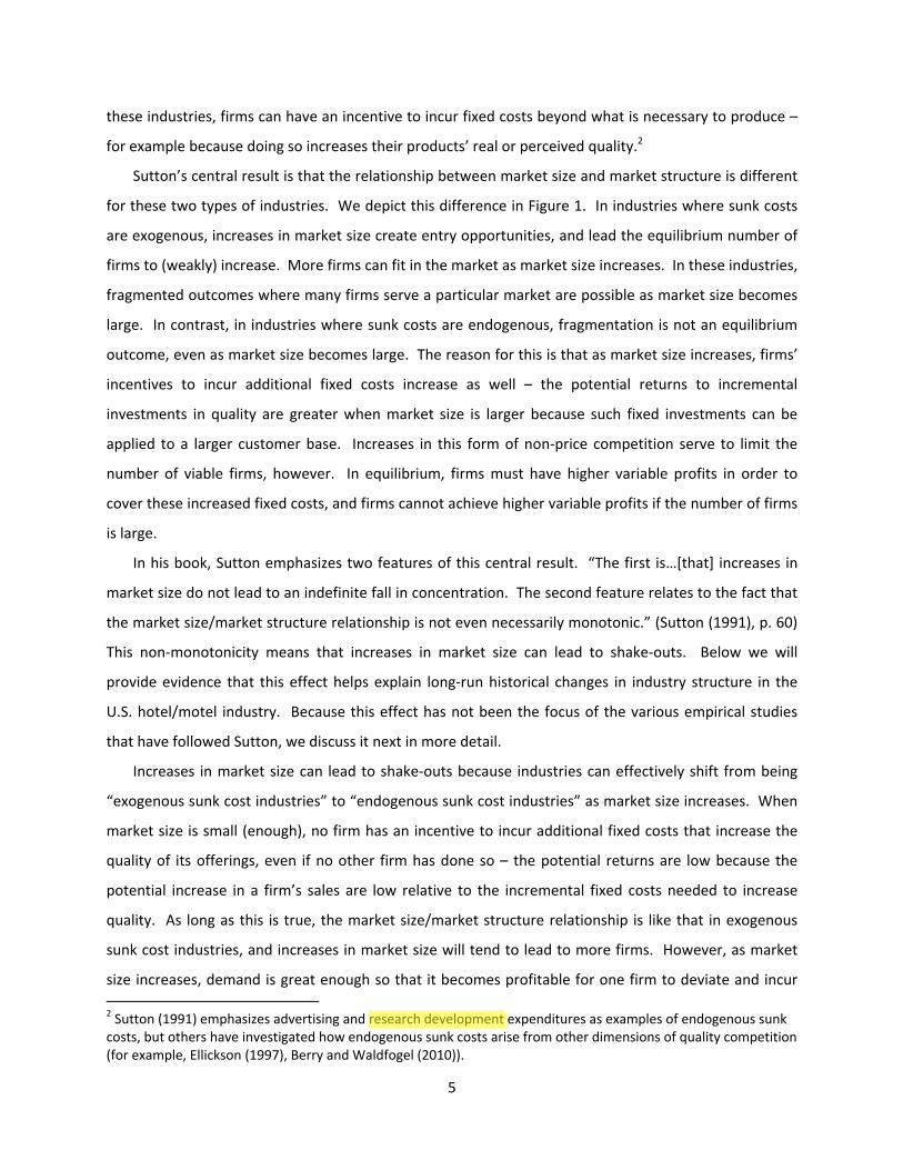
these industries, firms can have an incentive to incur fixed costs beyond what is necessary to produce – 

for example because doing so increases their products’ real or perceived quality.2  

Sutton’s central result is that the relationship between market size and market structure is different 

for these two types of industries.  We depict this difference in Figure 1.  In industries where sunk costs 

are exogenous, increases in market size create entry opportunities, and lead the equilibrium number of 

firms to (weakly) increase.  More firms can fit in the market as market size increases.  In these industries, 

fragmented outcomes where many firms serve a particular market are possible as market size becomes 

large.   In contrast,  in  industries where sunk costs are endogenous, fragmentation  is not an equilibrium 

outcome, even as market size becomes large.  The reason for this is that as market size increases, firms’ 

incentives  to  incur  additional  fixed  costs  increase  as  well  –  the  potential  returns  to  incremental 

investments  in quality are greater when market  size  is  larger because  such  fixed  investments  can be 

applied  to a  larger customer base.    Increases  in  this  form of non‐price competition  serve  to  limit  the 

number of  viable  firms, however.    In equilibrium,  firms must have higher  variable profits  in order  to 

cover these increased fixed costs, and firms cannot achieve higher variable profits if the number of firms 

is large. 

In his book, Sutton emphasizes two features of this central result.   “The first  is…[that]  increases  in 

market size do not lead to an indefinite fall in concentration.  The second feature relates to the fact that 

the market size/market structure relationship is not even necessarily monotonic.” (Sutton (1991), p. 60)  

This  non‐monotonicity means  that  increases  in market  size  can  lead  to  shake‐outs.    Below we will 

provide evidence  that  this effect helps explain  long‐run historical changes  in  industry structure  in  the 

U.S. hotel/motel  industry.   Because this effect has not been the focus of the various empirical studies 

that have followed Sutton, we discuss it next in more detail. 

Increases  in market size can  lead to shake‐outs because  industries can effectively shift from being 

“exogenous sunk cost industries” to “endogenous sunk cost industries” as market size increases.  When 

market size  is small (enough), no firm has an  incentive to  incur additional fixed costs that  increase the 

quality of  its offerings, even  if no other  firm has done so –  the potential returns are  low because  the 

potential  increase  in a  firm’s  sales are  low  relative  to  the  incremental  fixed  costs needed  to  increase 

quality.   As  long as this  is true, the market size/market structure relationship  is  like that  in exogenous 

sunk cost  industries, and  increases  in market size will tend to  lead to more firms.   However, as market 

size  increases, demand  is great enough so that  it becomes profitable for one firm to deviate and  incur 

                                                            2 Sutton (1991) emphasizes advertising and research development expenditures as examples of endogenous sunk costs, but others have investigated how endogenous sunk costs arise from other dimensions of quality competition (for example, Ellickson (1997), Berry and Waldfogel (2010)). 

6  

additional fixed costs toward attracting additional customers.   At this point, the competitive dynamics 

change and the market size/market structure relationship is no longer like that in exogenous sunk cost 

industries.    Once  firms  begin  to  compete  in  this  way  –  they  compete  on  quality  where  quality  is 

produced through fixed costs – fragmented outcomes that may have been possible even when market 

size was smaller are no longer equilibrium outcomes, and as market size increases further, the number 

of  firms  can decrease.    (See  Figure 1.)    Increases  in market  size  can  lead  to  shakeouts because  such 

increases can change an  industry’s competitive dynamics.   Such  increases enhance firms’  incentives to 

engage  in non‐price  competition, and a  consequence of  increased non‐price  competition  can be  that 

fewer firms can “fit  in the market” (i.e., have variable profits that at  least cover their fixed costs) than 

when market size was smaller and firms did not have as strong an incentive to compete in this way. 

As  Sutton  and  especially  Berry  and  Waldfogel  (2010)  have  emphasized,  the  fact  that  quality 

competition is in the form of fixed costs rather than variable costs is essential for Sutton’s central result.  

When quality competition takes the form of fixed costs, firms’ marginal costs are  independent of their 

quality, and a high quality firm has  low enough marginal costs so that  it can successfully compete not 

only  for  quality‐sensitive  customers,  but  also  for  less‐quality‐sensitive  customers.    This means  that 

increases in market size – even when these increases are only in more quality‐sensitive customers – can 

nevertheless  have  competitive  implications  for  incumbent  firms  that  serve  less‐quality‐sensitive 

customers.   By  increasing firms’  incentives to make fixed cost  investments  in their quality,  increases  in 

market  size  can  enhance  high‐quality  firms’  ability  to  compete  for  all  customers,  not  just  quality‐

sensitive  customers.    In  contrast,  when  quality  competition  takes  the  form  of  variable  costs,  the 

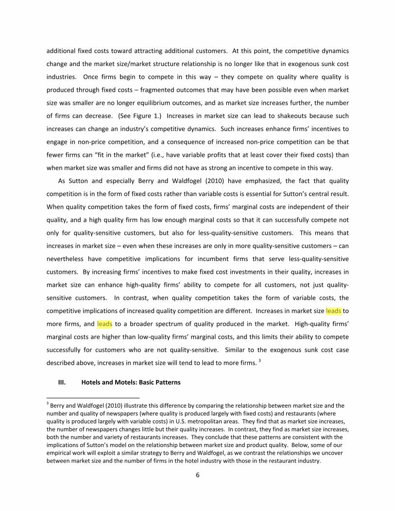
competitive implications of increased quality competition are different.  Increases in market size leads to 

more  firms,  and  leads  to  a broader  spectrum of quality produced  in  the market.   High‐quality  firms’ 

marginal costs are higher than low‐quality firms’ marginal costs, and this limits their ability to compete 

successfully  for  customers  who  are  not  quality‐sensitive.    Similar  to  the  exogenous  sunk  cost  case 

described above, increases in market size will tend to lead to more firms. 3 

III. Hotels and Motels: Basic Patterns 

                                                            3 Berry and Waldfogel (2010) illustrate this difference by comparing the relationship between market size and the number and quality of newspapers (where quality is produced largely with fixed costs) and restaurants (where quality is produced largely with variable costs) in U.S. metropolitan areas.  They find that as market size increases, the number of newspapers changes little but their quality increases.  In contrast, they find as market size increases, both the number and variety of restaurants increases.  They conclude that these patterns are consistent with the implications of Sutton’s model on the relationship between market size and product quality.  Below, some of our empirical work will exploit a similar strategy to Berry and Waldfogel, as we contrast the relationships we uncover between market size and the number of firms in the hotel industry with those in the restaurant industry.  

7  

  We begin by relating general trends in the U.S. hotel industry from the 1960s through the early 

1990s, the period of our sample.   These general trends come from published Census reports,  including 

County Business Patterns and the Economic Census.  Reports from the Economic Censuses provide key 

background  facts because, although  these generally only  took place every  five years,  the  surveys  the 

Census  sent  to  hotels  and  motels  asked  unusually  detailed  questions  about  hotels’  and  motels’ 

characteristics.  These background facts help shape our interpretations of our main analyses, which use 

data from County Business Patterns – which are annual and publicly available but do not contain detail 

about hotels’ and motels’ characteristics beyond their employment size. 

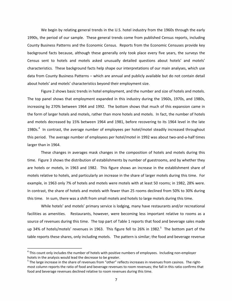
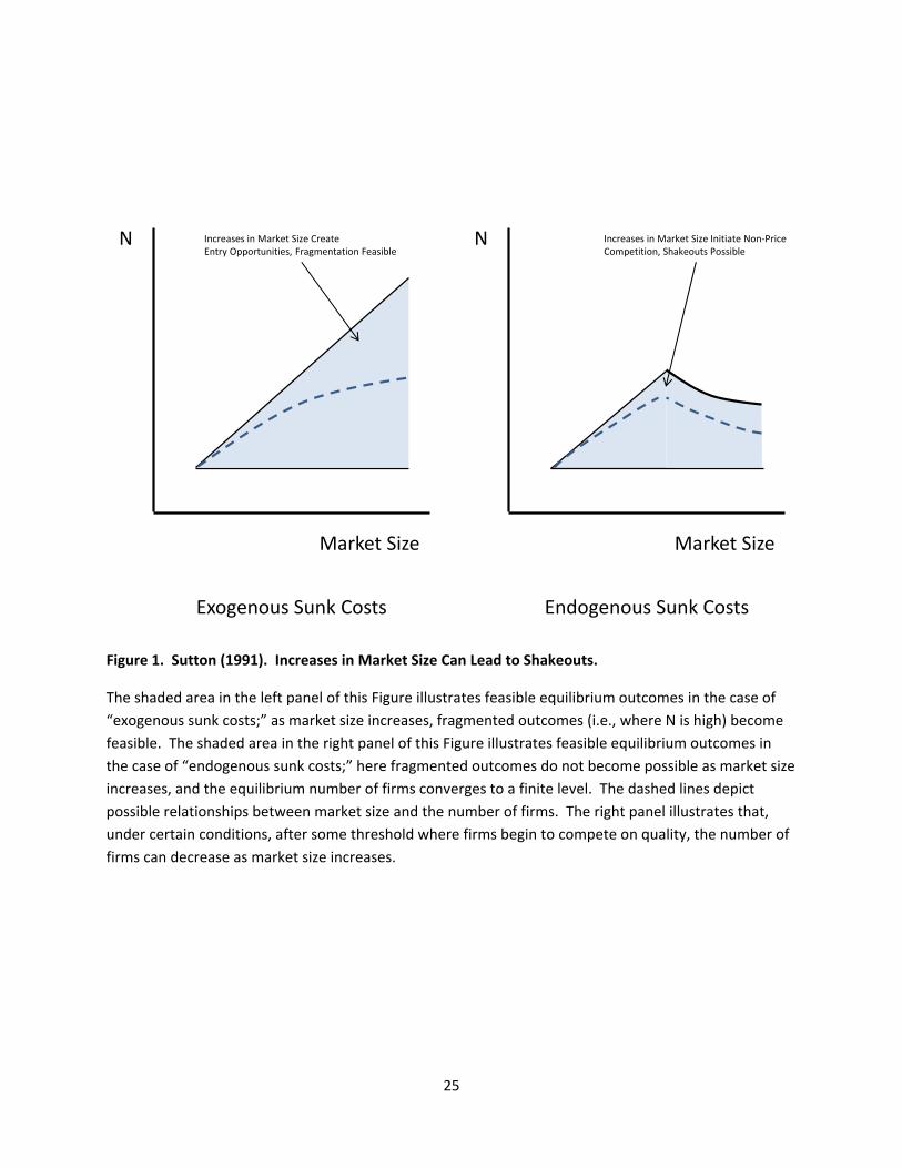
  Figure 2 shows basic trends in hotel employment, and the number and size of hotels and motels.  

The  top panel shows  that employment expanded  in  this  industry during  the 1960s, 1970s, and 1980s, 

increasing by 270% between 1964 and 1992.   The bottom shows that much of this expansion came  in 

the form of larger hotels and motels, rather than more hotels and motels.  In fact, the number of hotels 

and motels decreased by 15% between 1964 and 1981, before recovering  to  its 1964  level  in the  late 

1980s.4    In contrast, the average number of employees per hotel/motel steadily  increased throughout 

this period.  The average number of employees per hotel/motel in 1992 was about two‐and‐a‐half times 

larger than in 1964. 

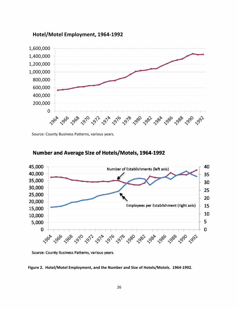
  These changes  in averages mask changes  in  the composition of hotels and motels during  this 

time.  Figure 3 shows the distribution of establishments by number of guestrooms, and by whether they 

are hotels or motels,  in 1963 and 1982.   This  figure  shows an  increase  in  the establishment  share of 

motels relative to hotels, and particularly an increase in the share of larger motels during this time.  For 

example, in 1963 only 7% of hotels and motels were motels with at least 50 rooms; in 1982, 28% were.  

In contrast, the share of hotels and motels with fewer than 25 rooms declined from 50% to 30% during 

this time.   In sum, there was a shift from small motels and hotels to large motels during this time. 

  While hotels’ and motels’ primary service is lodging, many have restaurants and/or recreational 

facilities  as  amenities.     Restaurants, however, were becoming  less  important  relative  to  rooms  as  a 

source of revenues during this time.  The top part of Table 1 reports that food and beverage sales made 

up 34% of hotels/motels’ revenues  in 1963.   This  figure  fell  to 26%  in 1982.5   The bottom part of  the 

table reports these shares, only including motels.   The pattern is similar; the food and beverage revenue 

                                                            4 This count only includes the number of hotels with positive numbers of employees.  Including non‐employer hotels in the analysis would lead the decrease to be greater. 5 The large increase in the share of revenues from “other” reflects increases in revenues from casinos.  The right‐most column reports the ratio of food and beverage revenues to room revenues; the fall in this ratio confirms that food and beverage revenues declined relative to room revenues during this time. 

8  

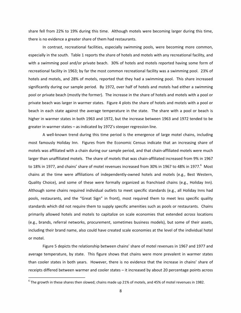
share fell from 22% to 19% during this time.   Although motels were becoming  larger during this time, 

there is no evidence a greater share of them had restaurants. 

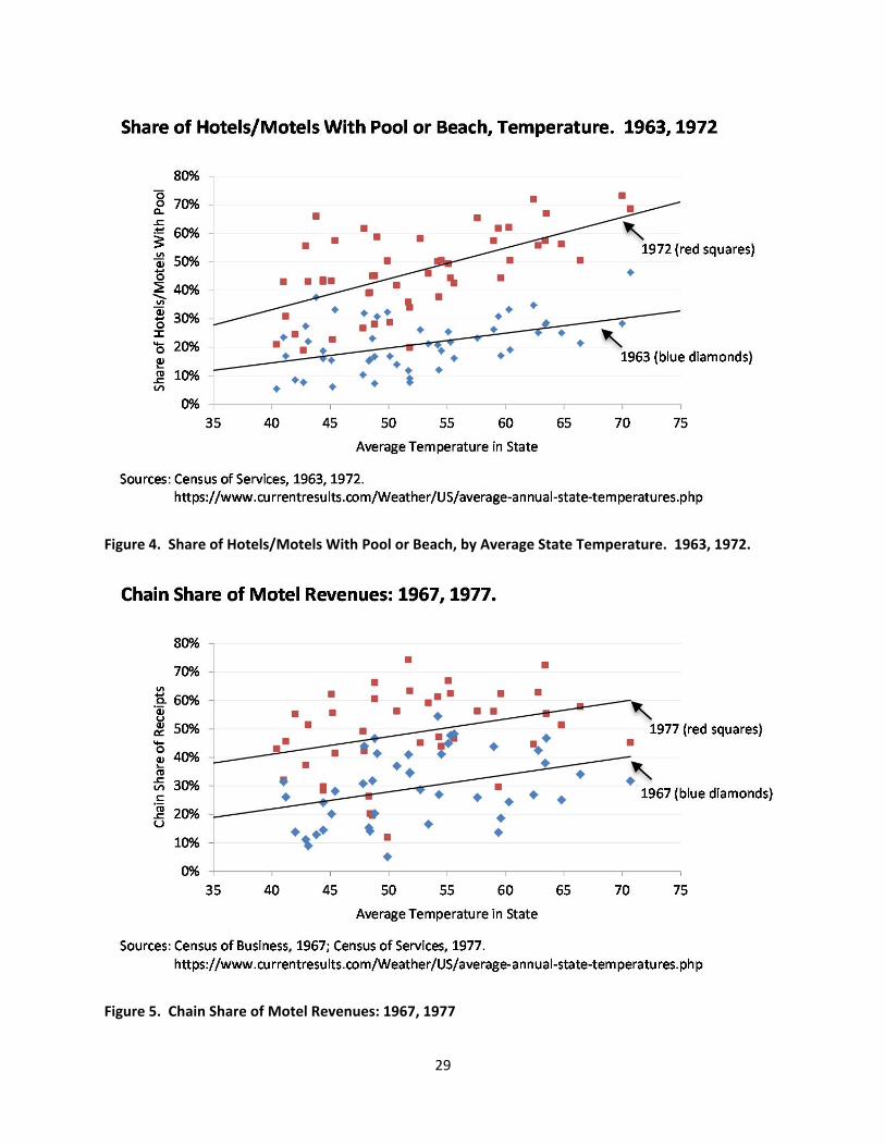
  In  contrast,  recreational  facilities, especially  swimming pools, were becoming more  common, 

especially in the south.  Table 1 reports the share of hotels and motels with any recreational facility, and 

with a swimming pool and/or private beach.   30% of hotels and motels reported having some form of 

recreational facility in 1963; by far the most common recreational facility was a swimming pool.  23% of 

hotels and motels, and 28% of motels, reported that they had a swimming pool.   This share  increased 

significantly during our sample period.   By 1972, over half of hotels and motels had either a swimming 

pool or private beach (mostly the former).  The increase in the share of hotels and motels with a pool or 

private beach was larger in warmer states.  Figure 4 plots the share of hotels and motels with a pool or 

beach  in each  state against  the average  temperature  in  the  state.   The  share with a pool or beach  is 

higher in warmer states in both 1963 and 1972, but the increase between 1963 and 1972 tended to be 

greater in warmer states – as indicated by 1972’s steeper regression line.  

A well‐known  trend during  this  time period  is  the emergence of  large motel chains,  including 

most  famously Holiday  Inn.    Figures  from  the  Economic  Census  indicate  that  an  increasing  share  of 

motels was affiliated with a chain during our sample period, and that chain‐affiliated motels were much 

larger than unaffiliated motels.  The share of motels that was chain‐affiliated increased from 9% in 1967 

to 18% in 1977, and chains’ share of motel revenues increased from 30% in 1967 to 48% in 1977.6  Most 

chains  at  the  time were  affiliations  of  independently‐owned  hotels  and motels  (e.g.,  Best Western, 

Quality  Choice),  and  some  of  these were  formally  organized  as  franchised  chains  (e.g., Holiday  Inn).  

Although some chains required  individual outlets to meet specific standards  (e.g., all Holiday  Inns had 

pools,  restaurants,  and  the  “Great  Sign”  in  front), most  required  them  to meet  less  specific  quality 

standards which did not require them to supply specific amenities such as pools or restaurants.  Chains 

primarily  allowed hotels  and motels  to  capitalize on  scale  economies  that  extended  across  locations 

(e.g., brands,  referral networks, procurement,  sometimes business models), but  some of  their assets, 

including their brand name, also could have created scale economies at the level of the individual hotel 

or motel. 

Figure 5 depicts the relationship between chains’ share of motel revenues in 1967 and 1977 and 

average  temperature, by  state.   This  figure  shows  that  chains were more prevalent  in warmer  states 

than cooler states  in both years.   However,  there  is no evidence  that  the  increase  in chains’ share of 

receipts differed between warmer and cooler states – it increased by about 20 percentage points across 

                                                            6 The growth in these shares then slowed; chains made up 21% of motels, and 45% of motel revenues in 1982. 

9  

the temperature spectrum.   Whereas the share of hotels and motels with pools increased more in the 

south  than  in  the north during our  time period,  the  expansion of motel  chains during  this  time was 

similar in the south and north.7 

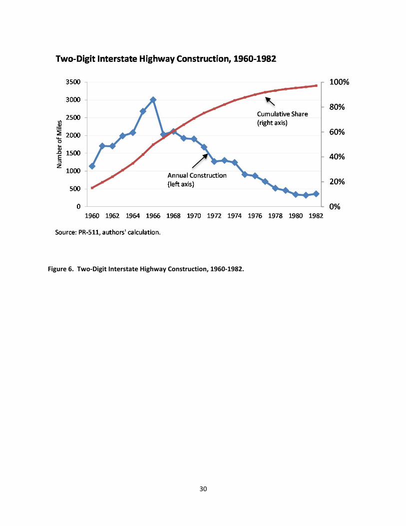
  Our analysis focuses on the relationship between changes in the number and size distribution of 

hotels and motels and  interstate highway openings.   Figure 6 summarizes the timing of the opening of 

two‐digit  interstate highways between 1960 and 1982.   About 15% of the mileage had opened by the 

end of 1960, 35% by the end of 1964, 75% by the end of 1971, and 97% by the end of 1982.  Highway 

openings peaked in 1965 and 1966, remained at over 1000 miles per year through 1974, then dwindled 

thereafter.    After  1983,  fewer  than  100 miles  per  year  of  new  two‐digit  interstate  highways  were 

opened.   Our data on hotels and motels extends  through  the early 1990s – allowing us  to  investigate 

long‐run relationships between highway openings and industry structure – but the highway openings we 

exploit are mainly in the 1960s and early 1970s. 

IV. Data 

  Our main data sources are  the same as  in Campbell and Hubbard  (2016).   We obtain county‐

level  data  on  hotel  employment,  the  total  number  of  hotels,  and  the  number  of  hotels  in  different 

employment‐size categories from the Bureau of the Census’ County Business Patterns, from 1964‐1992.8  

These data provide our main dependent variables, including the number and average employment size 

of hotels in U.S. counties.9 

We restrict our analysis to smaller counties where traffic patterns are relatively uncomplicated, and 

where one would expect  through  traffic  to be an  important  source of demand  for hotels – and  thus 

highway  completion would  be  an  economically  important  demand  shock.    Similar  to  Campbell  and 

Hubbard (2016), we use only counties with one one‐ or two‐digit Interstate highway and no three‐digit 

interstates  (which  eliminates most  large  cities  and  counties where  Interstates  intersect),  and  further 

eliminate  the  few  populous  counties  that  remain  by  dropping  those  whose  employment  exceeded 

                                                            7 Differences in the years in this Figure and Figure 4 reflect that the Economic Census’ survey forms changed from year to year; the Census did not ask about chain affiliation until 1967, and did not ask about recreational facilities after 1972. 8 Hereafter, to simplify language, we will use the term “hotels” to mean “hotels and motels.”  County Business Patterns does not distinguish between the two. 9 Before 1974, the Census reported the number of firms operating hotels in each county, rather than the number of hotels.  This has a small effect on our analysis because it is uncommon for firms to operate multiple hotels in the same county, in our sample counties.  (It is much more common for a chain to have multiple hotels in a county which are operated by separate franchisees.)  Below we describe how we account for this in our empirical framework.  Here and throughout, we will use the word “hotels” rather than the phrase “firms operating hotels” to discuss this variable, even though the latter is more accurate before 1974. 

10  

200,000  in 1992.   We  further eliminate counties where  the  Interstate passes  through but  there  is no 

exit.   We conduct our analysis on a balanced panel of 227 counties which satisfy these criteria and for 

which we observe the number of hotels in each of our sample years.10 

Along with  data  on  hotels, we  also  collect  analogous  data  on  two  other  industries:  “eating  and 

drinking places” (“EDPs;” i.e., restaurants and bars) and “gasoline retailing.”  We use these other data in 

“falsification  exercises”  to  investigate  the  hypothesis  that  the  relationships  we  observe  between 

highway openings and changes in industry structure in hotels reflect competitive effects that one would 

expect to observe in the hotel industry but not these other industries. 

  We combine these data with highly detailed data on Interstate Highway openings.  These come 

from the U.S. Department of Transportation’s “PR‐511” file.  We observe in these data the opening date 

of every mile of the Interstate Highway System.  We calculate from these data the two key independent 

variables  in our analysis.   One  is csmiit, the cumulative share of  interstate highway mileage  in county  i 

that was completed by the end of year t.   Because highways are completed and opened in segments, it 

is  typical  for a part of a highway  to be opened  in a county,  then  the  rest of  it  some  time  later.   This 

variable allows us to assess the effects of highway openings in a county on the number and size of hotels 

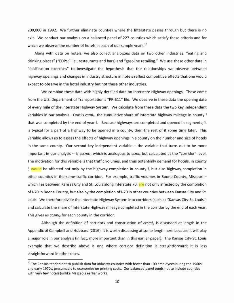
in  the  same  county.   Our  second  key  independent  variable –  the  variable  that  turns out  to be more 

important in our analysis ‐‐ is ccsmiit, which is analogous to csmiit but calculated at the “corridor” level.  

The motivation for this variable is that traffic volumes, and thus potentially demand for hotels, in county 

i, would be affected not only by  the highway completion  in county  i, but also highway completion  in 

other counties  in  the same  traffic corridor.   For example,  traffic volumes  in Boone County, Missouri – 

which lies between Kansas City and St. Louis along Interstate 70, are not only affected by the completion 

of I‐70 in Boone County, but also by the completion of I‐70 in other counties between Kansas City and St. 

Louis.  We therefore divide the Interstate Highway System into corridors (such as “Kansas City‐St. Louis”) 

and calculate the share of Interstate Highway mileage completed in the corridor by the end of each year.  

This gives us ccsmiit for each county in the corridor. 

  Although  the  definition  of  corridors  and  construction  of  ccsmiit  is  discussed  at  length  in  the 

Appendix of Campbell and Hubbard (2016), it is worth discussing at some length here because it will play 

a major role in our analysis (in fact, more important than in this earlier paper).  The Kansas City‐St. Louis 

example  that  we  describe  above  is  one  where  corridor  definition  is  straightforward;  it  is  less 

straightforward in other cases. 

                                                            10 The Census tended not to publish data for industry‐counties with fewer than 100 employees during the 1960s and early 1970s, presumably to economize on printing costs.  Our balanced panel tends not to include counties with very few hotels (unlike Mazzeo’s earlier work). 

11  

  The  first  step  in  defining  corridors  is  determining  corridor  endpoints  (i.e.,  the  nodes  of  the 

network).  We found that one useful way of doing so is simply by looking at a map of the United States 

in a road atlas, and using the cities that are denoted in bold.  These cities all have population of at least 

100,000 people  (as of 1996, the date of the map we used).    In  large metropolitan areas where both a 

central city and one or more surrounding cities have more than 100,000 population, the bolded city only 

generally  includes the central city  (e.g., Los Angeles, but not Pasadena).   We then chose an  important 

interstate highway junction as the exact beginning/endpoint of the corridor.  In some cases highways do 

not end  in cities  (for example,  they end at  the Canadian border, or an east‐west highway ends at  the 

junction  of  a  north‐south  highway);  in  these  cases,  the  end  of  the  highway  served  as  the  corridor 

endpoint. 

  The  second  step  of  the  process  is  assigning  highway  segments  to  corridors.    This  is 

straightforward  in cases  such as Boone County where  the highway  is only part of one corridor but  is 

more  complicated  in  other  cases,  such  as when  there  is  a  “fork  in  the  road”  between  two  corridor 

endpoints, or when highways merge and  then separate.      In such cases,  the highway segments  in  the 

“trunks” are part of multiple corridors  that  involve different branches.   For example, going west  from 

Tucson, Arizona, Interstate 10 splits into two highways (Interstate 8, and the continuation of Interstate 

10).  The “trunk” between Tucson and this split is part of two corridors: Tucson‐San Diego and Tucson‐

Phoenix.     For counties along  these  trunks, we calculate a single corridor completion measure by  first 

calculating  the  cumulative  share  of  construction  along  each  corridor,  then weighting  each  of  these 

corridors by the traffic volume on each of the branches, evaluated at a point as close as possible to the 

trunk.11  

  Finally,  we  collect  data  on  temperatures  by  county  from  the  North  America  Land  Data 

Assimilation System  (NLDAS).12   These  report  that average high and  low  temperatures  in each of  the 

counties  in our  sample, where  the averages are  taken  from 1979‐2010 over 14x14 kilometer  regions 

that span each county.   From this, we construct an “average temperature” variable for each county by 

simply  taking  the mean of  the average high and  low  temperature.   Average  temperature  ranges  from 

about 40 degrees to about 75 degrees across the counties in our sample; the mean across counties is 55 

degrees. 

Basic Patterns In Our Sample 

                                                            11 For example, if the branch on the Tucson‐Phoenix corridor had twice as much traffic as that on the Tucson‐San Diego corridor, the former would receive a 2/3 weight and the latter a 1/3 weight. 12 https://wonder.cdc.gov/nasa‐nldas.html 

12  

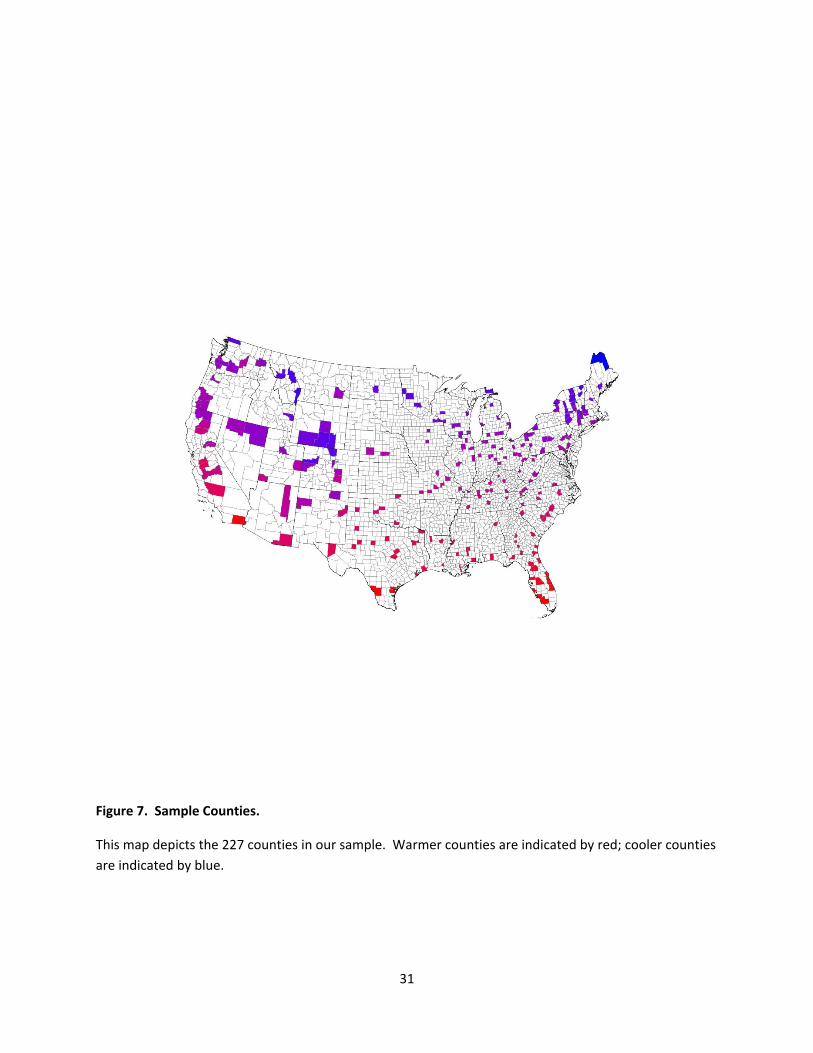
  Figure  7  depicts  the  counties  in  our  sample, with  average  temperatures  depicted  on  a  scale 

ranging from blue to red.  This figure shows that our counties come from all regions of the United States.  

Though none of these counties have large cities, many have smaller cities (e.g., Anniston, AL; Modesto, 

CA; New London, CT). 

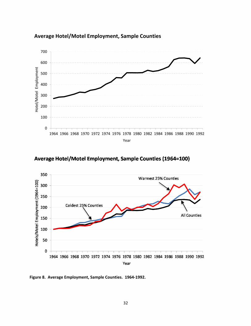
  Figure 8 shows county‐level employment at hotels in our sample counties.  The top panel shows 

that on average, employment  increased  from around 300  in 1964  to over 600  in 1992.   The bottom 

panel  breaks  out  the  coldest  25%  and  warmest  25%  of  counties  in  our  sample,  and  normalizes 

employment in each of these two groups to their 1964 level.  The trends in these two groups are similar 

to each other and similar to the average across our sample; total hotel employment slightly more than 

doubled during this time period.   This suggests that the supply expansion during  this  time period was 

similar, irrespective of whether the county was in the north or south. 

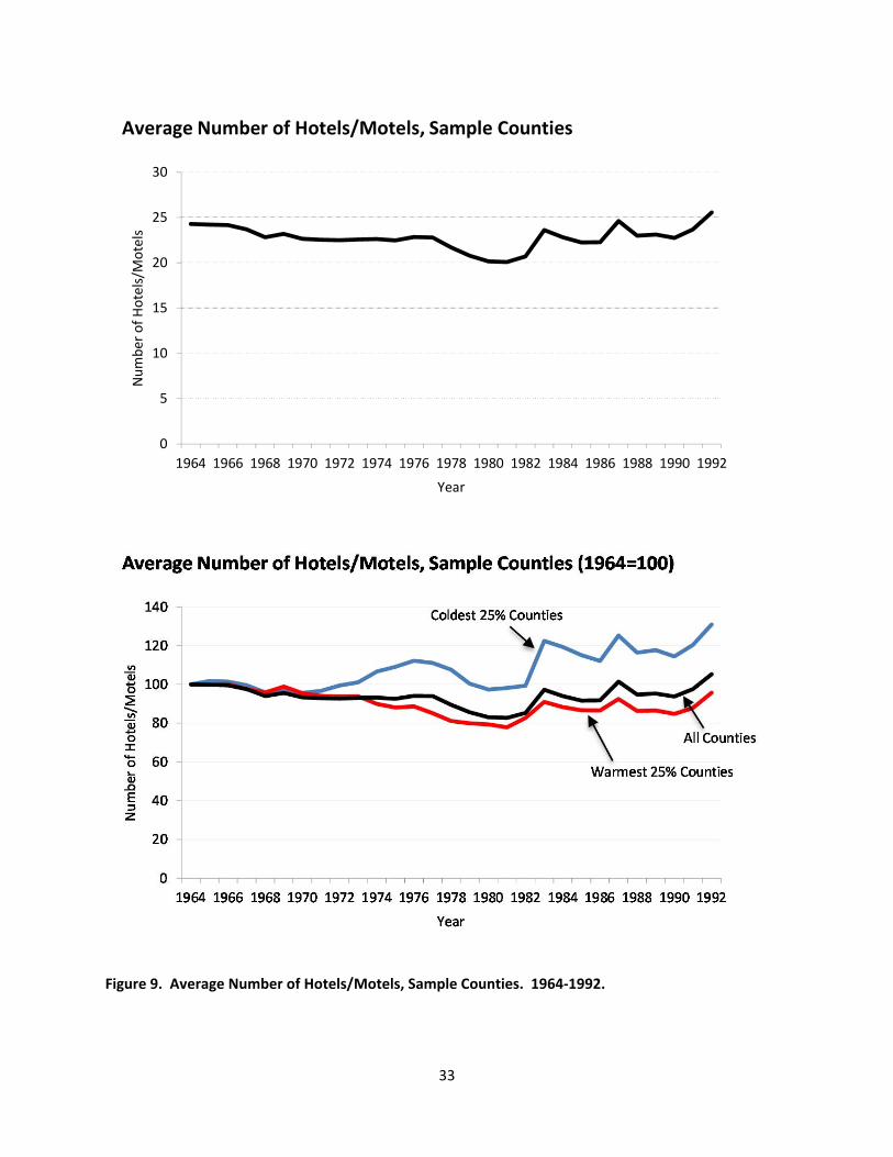
  Figure 9 shows the average number of hotels in our sample counties.  The top panel shows that 

this declined by 15‐20% between 1964 and 1981, then rose by the same amount between 1981‐1992.  

This pattern  is similar to that  in the national data we discussed above.   The bottom panel shows that, 

unlike  the patterns we  reported  in Figure 8  for employment at hotels,  the changes  in  the number of 

hotels differ  in cold and warm counties.   The number of hotels  increased during our sample by more 

than 20% in cold counties.  It decreased by about 20% between 1964 and 1981 in warm counties, then 

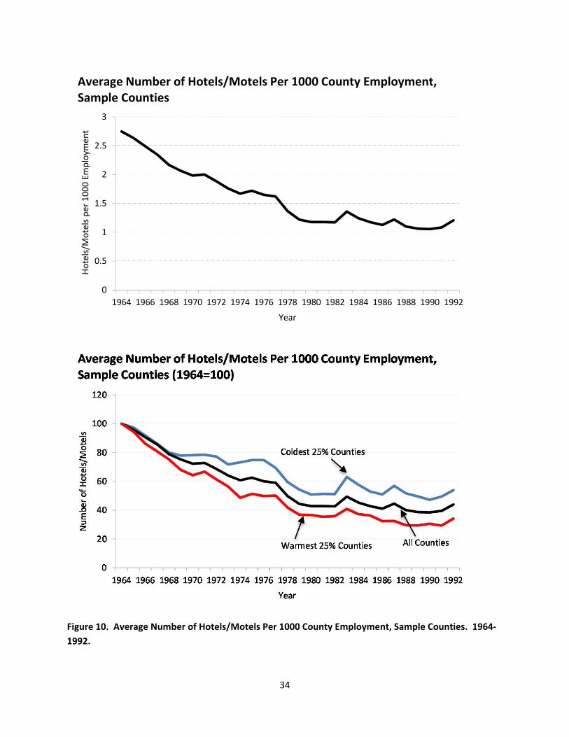
recovered  to  close  to  its 1964  level by 1992.    Figure 10  reports  analogous patterns, normalizing  the 

number of hotels by  a  county’s  employment; much of our  regression  analysis will use  this measure, 

which normalizes by the size of the county.  The top panel shows that, on average, the number of hotels 

per 1000 county employment declines by about one‐half during our sample period;  the bottom panel 

shows that this decline is greater in warm counties than cold counties. 

  Combined, Figures 8‐10 provide evidence that although the supply expansion was similar in cold 

and  warm  counties  during  our  sample  period,  industry  structure  evolved  differently.    There  was  a 

decline in the number of hotels in our warm counties, and an increase in our cold counties. 

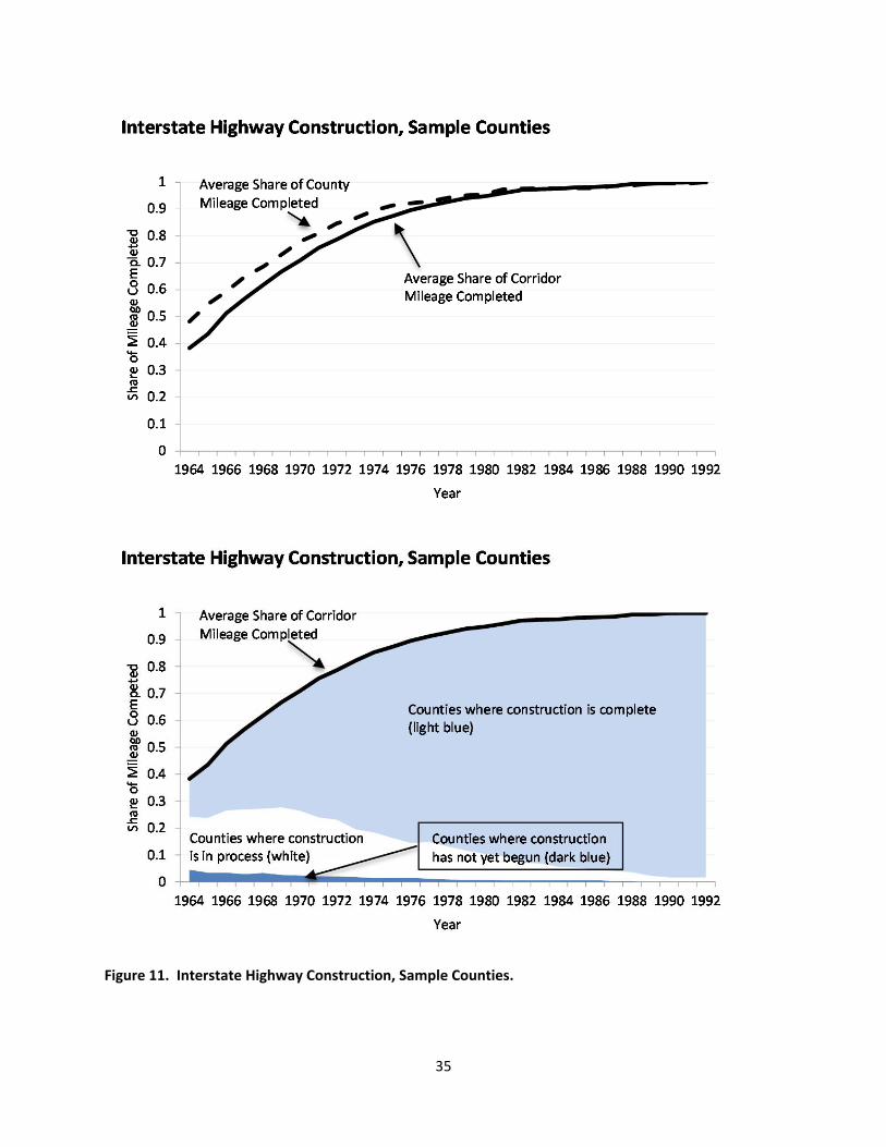
  Figure 11 depicts interstate highway construction in our sample counties.  In the top panel, the 

dashed line depicts yearly averages of csmit, the share of interstate highway mileage in the county that 

was  completed  by  the  end  of  year  t.    It  indicates  that,  on  average,  about  half  of  the mileage was 

completed by the end of 1964, about 80% by the end of 1971, and well over 90% by the end of 1980.  

The solid line depicts yearly averages of ccsmit, the share of interstate highway mileage in the county’s 

corridor that was completed by the end of year t.   This shows a similar pattern, but  is  lower than the 

dashed  line  in most  of  our  sample  period.    Thus,  highway  construction  in  our  sample  counties was 

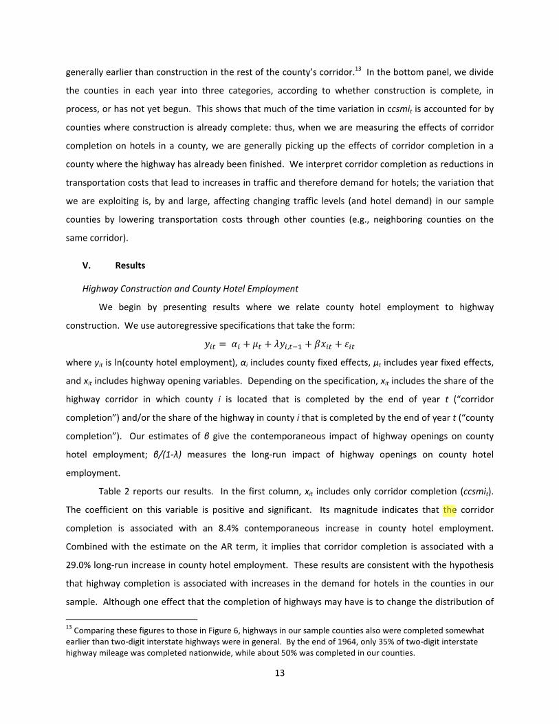
13  

generally earlier than construction in the rest of the county’s corridor.13  In the bottom panel, we divide 

the  counties  in  each  year  into  three  categories,  according  to  whether  construction  is  complete,  in 

process, or has not yet begun.  This shows that much of the time variation in ccsmit is accounted for by 

counties where construction  is already complete: thus, when we are measuring the effects of corridor 

completion on hotels  in a county, we are generally picking up  the effects of corridor completion  in a 

county where the highway has already been finished.  We interpret corridor completion as reductions in 

transportation costs that lead to increases in traffic and therefore demand for hotels; the variation that 

we are exploiting  is, by and  large, affecting  changing  traffic  levels  (and hotel demand)  in our  sample 

counties  by  lowering  transportation  costs  through  other  counties  (e.g.,  neighboring  counties  on  the 

same corridor). 

V. Results 

Highway Construction and County Hotel Employment 

  We  begin  by  presenting  results  where  we  relate  county  hotel  employment  to  highway 

construction.  We use autoregressive specifications that take the form: 

,  

where yit is ln(county hotel employment), αi includes county fixed effects, µt includes year fixed effects, 

and xit includes highway opening variables.  Depending on the specification, xit includes the share of the 

highway  corridor  in  which  county  i  is  located  that  is  completed  by  the  end  of  year  t  (“corridor 

completion”) and/or the share of the highway in county i that is completed by the end of year t (“county 

completion”).   Our estimates of β give  the  contemporaneous  impact of highway openings on  county 

hotel  employment;  β/(1‐λ)  measures  the  long‐run  impact  of  highway  openings  on  county  hotel 

employment. 

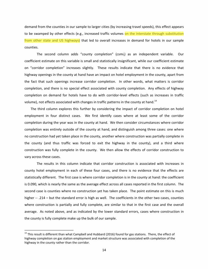
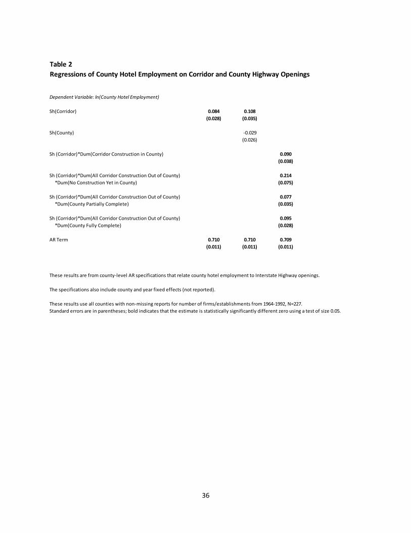
  Table 2  reports our  results.    In  the  first column, xit  includes only corridor completion  (ccsmit).  

The  coefficient  on  this  variable  is  positive  and  significant.    Its magnitude  indicates  that  the  corridor 

completion  is  associated  with  an  8.4%  contemporaneous  increase  in  county  hotel  employment.  

Combined with  the estimate on  the AR  term,  it  implies  that  corridor  completion  is associated with a 

29.0% long‐run increase in county hotel employment.  These results are consistent with the hypothesis 

that highway completion  is associated with  increases  in  the demand  for hotels  in  the counties  in our 

sample.  Although one effect that the completion of highways may have is to change the distribution of 

                                                            13 Comparing these figures to those in Figure 6, highways in our sample counties also were completed somewhat earlier than two‐digit interstate highways were in general.  By the end of 1964, only 35% of two‐digit interstate highway mileage was completed nationwide, while about 50% was completed in our counties. 

14  

demand from the counties in our sample to larger cities (by increasing travel speeds), this effect appears 

to be swamped by other effects  (e.g.,  increased traffic volumes on the  interstate through substitution 

from other  state  and US highways)  that  led  to overall  increases  in demand  for hotels  in our  sample 

counties. 

  The  second  column  adds  “county  completion”  (csmit)  as  an  independent  variable.    Our 

coefficient estimate on this variable is small and statistically insignificant, while our coefficient estimate 

on  “corridor  completion”  increases  slightly.    These  results  indicate  that  there  is  no  evidence  that 

highway openings in the county at hand have an impact on hotel employment in the county, apart from 

the  fact  that  such  openings  increase  corridor  completion.    In  other words, what matters  is  corridor 

completion, and there  is no special effect associated with county completion.   Any effects of highway 

completion  on  demand  for  hotels  have  to  do with  corridor‐level  effects  (such  as  increases  in  traffic 

volume), not effects associated with changes in traffic patterns in the county at hand.14    

The  third column explores  this  further by considering  the  impact of corridor completion on hotel 

employment  in  four  distinct  cases.    We  first  identify  cases  where  at  least  some  of  the  corridor 

completion during the year was in the county at hand.  We then consider circumstances where corridor 

completion was entirely outside of the county at hand, and distinguish among three cases: one where 

no construction had yet taken place in the county, another where construction was partially complete in 

the  county  (and  thus  traffic  was  forced  to  exit  the  highway  in  the  county),  and  a  third  where 

construction was  fully complete  in  the county.   We  then allow  the effects of corridor construction  to 

vary across these cases. 

  The  results  in  this  column  indicate  that  corridor  construction  is  associated with  increases  in 

county hotel  employment  in  each of  these  four  cases,  and  there  is no  evidence  that  the  effects  are 

statistically different.  The first case is where corridor completion is in the county at hand: the coefficient 

is 0.090, which is nearly the same as the average effect across all cases reported in the first column.  The 

second case is counties where no construction yet has taken place.  The point estimate on this is much 

higher ‐‐ .214 – but the standard error is high as well.  The coefficients in the other two cases, counties 

where construction  is partially and  fully complete, are  similar  to  that  in  the  first case and  the overall 

average.   As noted above, and as  indicated by the  lower standard errors, cases where construction  in 

the county is fully complete make up the bulk of our sample. 

                                                            14 This result is different than what Campbell and Hubbard (2016) found for gas stations.  There, the effect of highway completion on gas station employment and market structure was associated with completion of the highway in the county rather than the corridor. 

15  

  Together,  these  results  are  consistent with  the  hypothesis  that demand  increases  associated 

with  highway  completion  are  related  to  increased  traffic  volumes  in  the  corridor,  and  not  other 

potentially more localized effects.  The effect of highway completion in county A on hotel employment 

in county B (another county on the same corridor) is no different than the effect of highway completion 

in county B on hotel employment in county B.  Furthermore, the effect of highway completion in county 

A on county B exists both when  the highway  in county B  is  fully complete and when  it has yet  to be 

started, and the effect is not significantly different. 

Highway Completion and Industry Structure in Hotels 

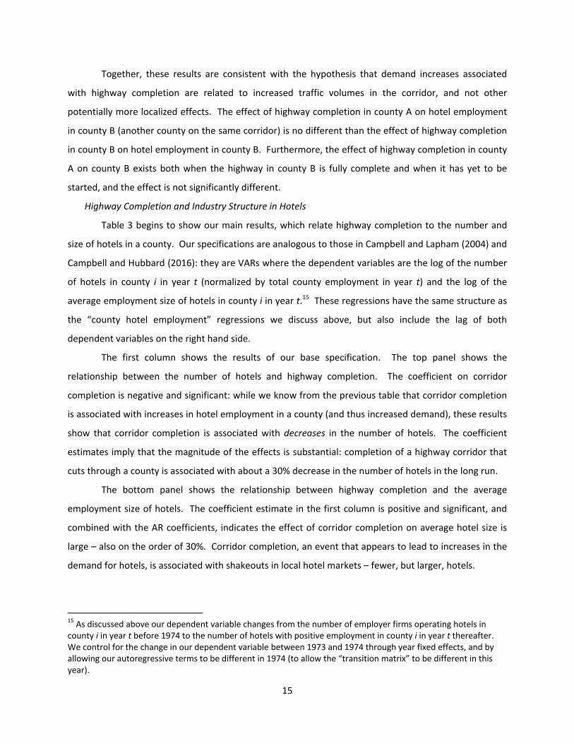
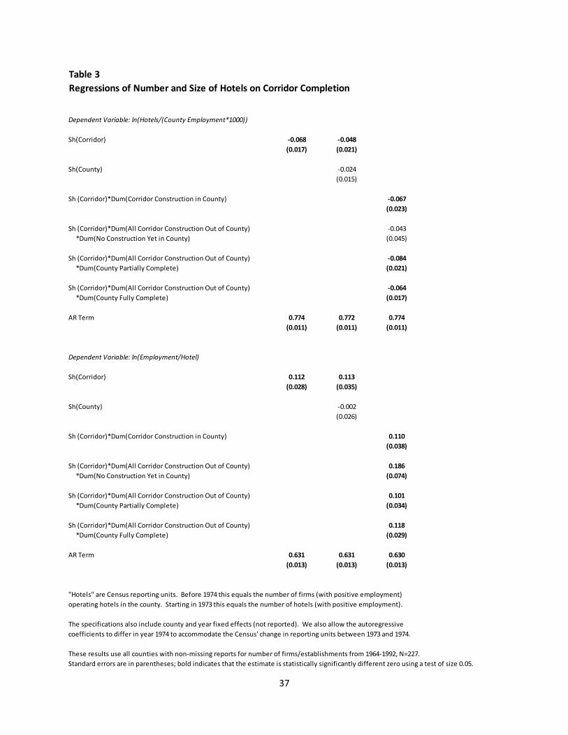
  Table 3 begins to show our main results, which relate highway completion to the number and 

size of hotels in a county.  Our specifications are analogous to those in Campbell and Lapham (2004) and 

Campbell and Hubbard (2016): they are VARs where the dependent variables are the log of the number 

of hotels  in  county  i  in  year  t  (normalized by  total  county employment  in  year  t)  and  the  log of  the 

average employment size of hotels in county i in year t.15  These regressions have the same structure as 

the  “county  hotel  employment”  regressions  we  discuss  above,  but  also  include  the  lag  of  both  

dependent variables on the right hand side.   

  The  first  column  shows  the  results  of  our  base  specification.    The  top  panel  shows  the 

relationship  between  the  number  of  hotels  and  highway  completion.    The  coefficient  on  corridor 

completion is negative and significant: while we know from the previous table that corridor completion 

is associated with increases in hotel employment in a county (and thus increased demand), these results 

show  that  corridor  completion  is associated with decreases  in  the number of hotels.   The  coefficient 

estimates  imply that the magnitude of the effects  is substantial: completion of a highway corridor that 

cuts through a county is associated with about a 30% decrease in the number of hotels in the long run. 

  The  bottom  panel  shows  the  relationship  between  highway  completion  and  the  average 

employment size of hotels.   The coefficient estimate  in the first column  is positive and significant, and 

combined with the AR coefficients,  indicates the effect of corridor completion on average hotel size  is 

large – also on the order of 30%.  Corridor completion, an event that appears to lead to increases in the 

demand for hotels, is associated with shakeouts in local hotel markets – fewer, but larger, hotels. 

                                                            15 As discussed above our dependent variable changes from the number of employer firms operating hotels in county i in year t before 1974 to the number of hotels with positive employment in county i in year t thereafter.   We control for the change in our dependent variable between 1973 and 1974 through year fixed effects, and by allowing our autoregressive terms to be different in 1974 (to allow the “transition matrix” to be different in this year). 

16  

  The other two columns in this table are analogous to those in the county hotel employment in 

Table 2.   Like  in  these other  regressions,  there  is no evidence  that  these effects differ when corridor 

completion  is  in the county at hand, or differ by the extent to which  the highway  is completed  in the 

county at hand.   This  fact  shapes our  interpretation of  the  relationship between highway completion 

and shakeouts.  If our results only reflected that highway completion in county A led to a decline in the 

number of hotels  in  county A,  then  shakeouts  associated with highway  completion  could  reflect  the 

impact  that  new  highways  have  on  industry  structure  through  changes  in  local  traffic  patterns:  for 

example,  they could change  local markets’ competitive dynamics by making hotel  locations near exits 

much desirable than other locations.  However, we find that the effect of highway completion in county 

A  leads to a similar decline  in the number of hotels  in county A and  in other counties along the same 

corridor –  including counties where the highway was completed years before.   We therefore conclude 

that  the  relationship  between  highway  completion  and  shakeouts  is  instead  related  to  highway 

completion’s effect on traffic  levels, and thus demand for  lodging  in the county – an effect that would 

exist regardless of whether the highway was completed  in the county at hand or  in other counties on 

the same corridor. 

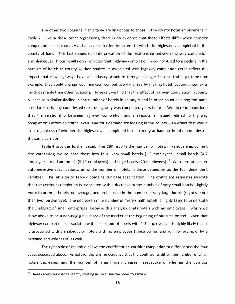
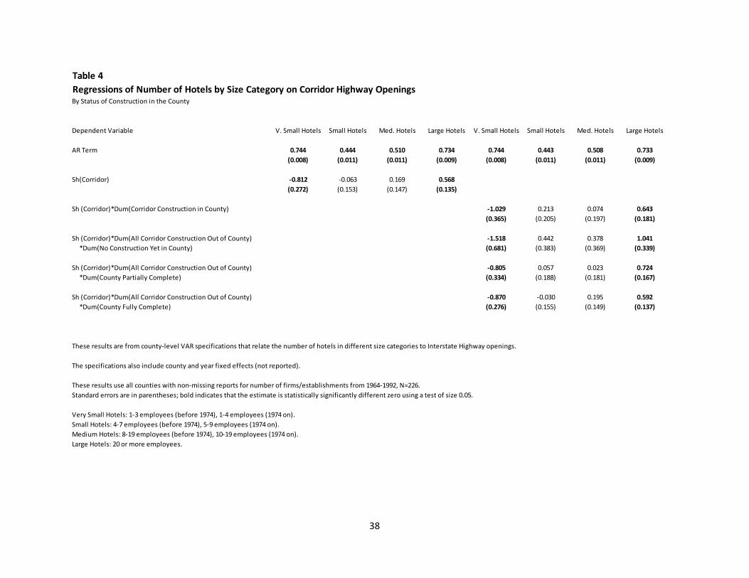
  Table 4 provides further detail.   The CBP reports the number of hotels  in various employment 

size  categories;  we  collapse  these  into  four:  very  small  hotels  (1‐3  employees),  small  hotels  (4‐7 

employees), medium hotels  (8‐19 employees) and  large hotels  (20 employees).16   We  then run vector 

autoregressive  specifications,  using  the  number  of  hotels  in  these  categories  as  the  four  dependent 

variables.   The  left  side of Table 4 contains our base  specification.   The coefficient estimates  indicate 

that the corridor completion  is associated with a decrease  in the number of very small hotels (slightly 

more than three hotels, on average) and an  increase  in the number of very  large hotels (slightly more 

than two, on average).  The decrease in the number of “very small” hotels is highly likely to understate 

the  shakeout of  small enterprises, because  this analysis omits hotels with no employees – which we 

show above to be a non‐negligible share of the market at the beginning of our time period.  Given that 

highway completion is associated with a shakeout of hotels with 1‐3 employees, it is highly likely that it 

is associated with a  shakeout of hotels with no employees  (those owned and  run,  for example, by a 

husband and wife team) as well. 

  The right side of the table allows the coefficient on corridor completion to differ across the four 

cases described above.  As before, there is no evidence that the coefficients differ: the number of small 

hotels  decreases,  and  the  number  of  large  firms  increases,  irrespective  of  whether  the  corridor 

                                                            16 These categories change slightly starting in 1974; see the notes to Table 4. 

17  

completion was  in the county at hand, and  irrespective of how much of the highway  in the county at 

hand had been completed. 

Non‐Price Competition and Shake‐Outs: Is the Shakeout Greater in Warmer Places? 

  Summarizing,  Tables  2‐4  show  our  central  empirical  facts:  the  completion  of  highways  leads 

hotel employment to increase, and leads to fewer but larger firms.  The following two sections provide 

evidence on how these results reflect nonprice competition in this industry. 

  Our  analytical  framework  above  showed  that,  in  a  homogeneous  good  industry,  increases  in 

demand should not lead to shakeouts: the number of firms should (weakly) increase, not decrease.  In a 

differentiated product market, however,  the  firms’  competitive  responses  to positive demand  shocks 

can  lead the equilibrium number of firms to decrease.    In particular,  if there  is vertical differentiation, 

and quality is produced with fixed costs, then demand increases can lead to the entry of scale‐intensive 

high quality firms that can price low enough not only to attract customers with a high willingness to pay 

for quality, but also those with a lower willingness to pay for quality.  This competitive response, in turn, 

can  lead  to  the  shake‐out of  smaller,  low‐quality  firms and  to a net decrease  in  the  total number of 

firms. 

  Our  discussion  above  described  how  one  quality  amenity  that  was  becoming  increasingly 

prevalent at U.S. hotels during our time period was a swimming pool.   Supplying this amenity  involved 

almost entirely fixed costs – the cost of supplying this amenity was the same, irrespective of how many 

guests would ultimately utilize  it.   However, the quality enhancement associated with this  investment 

varied with the local climate – it was higher in warmer places because the pool was usable more months 

out of  the year.    If  the shakeout associated with highway completion  reflected non‐price competition 

associated with  swimming  pools  (or  other  less  common  outdoor  amenities  such  as  a  playground  or 

putting green), one would expect the shakeout to be greater in warmer places. 

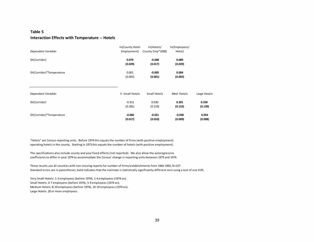
  We  test  this  proposition  in  Table  5  by  interacting  corridor  completion  with  the  average 

temperature  in each of our sample counties.17   The top panel shows regressions where the dependent 

variable is (logged) county hotel employment, the number of hotels, and the average employment size 

of hotels.   The  interaction coefficient  in  the  first  column  is essentially  zero:  the  relationship between 

corridor completion and county hotel employment  is  just as strong  in cold places as  in warmer places.  

There is thus no evidence that highway completion leads to larger increases in demand for hotels in the 

warm counties in our sample than the cold counties in our sample.  The coefficients in the second and 

                                                            17 More precisely, we interact it with (temperature‐55), so that the uninteracted coefficient corresponds to the effect of highway completion for the county in our sample with average temperature. 

18  

third columns show that the change in industry structure is very different.  The interaction coefficient in 

the  second  column  is  negative,  significant,  and  economically  large.    It  implies  that  the  shakeout 

associated  with  highway  completion  was  much  greater  in  warmer  places.    The  magnitudes  imply 

essentially  no  change  in  the  number  of  hotels  in  our  cooler  counties  (counties  with  an  average 

temperature around 45 degrees), but large decrease – twice the average effect – in our warmer counties 

(counties with an average temperature of around 65 degrees).   The  interaction coefficient  in the right 

column  suggests  that  the  increase  in hotel  size was  also more pronounced  in warmer  counties  than 

cooler counties,  though  the coefficient  is not quite statistically different  from zero using a  test of size 

0.05. 

  We show these results graphically in Figure 12.  The top panel shows the relationship between 

corridor  completion  and  county  hotel  employment.    The  long  run  effect more  than  20%,  and  is  not 

statistically different  for cold and warm counties;  if anything, the effect  is  larger  for warmer counties.  

The bottom panel shows the relationship between corridor completion and the number of hotels.  There 

is no effect in cold counties, but a large effect – on the order of a 40% decrease – in warm counties. 

  The bottom panel of Table 5 shows  interaction specifications where the dependent variable  is 

the number of hotels in different employment size categories.  These results show are similar to those in 

the top panel, and imply that the decrease in very small hotels, and increase in large hotels, was much 

greater in our warmer counties than in our cooler counties.  Figure 13 shows this graphically.  In warm 

counties, there is an increase in the number of large hotels and a correspondingly larger decrease in the 

number of small hotels.  In contrast, in cold counties, corridor completion has little effect on the number 

of hotels  in any of  these  size categories.    In particular, we  find no evidence  that corridor completion 

leads to more large hotels, or to a shake‐out of very small hotels.  The adjustment in industry structure 

was very different in warm places than cold places. 

  Together,  these  results provide  support  for  the proposition  that non‐price  competition  in  the 

form of  fixed costs explains why highway completion  led  to a shakeout  in  the number of hotels.   Our 

evidence indicates that highway completion led to increases in the demand for hotels in both cool and 

warm counties in our sample – in both North Dakota and Georgia.  But it led to fewer, but larger, hotels 

only in the warm places, but not the cold places. 

  Above we emphasize one form of quality competition that would lead to shakeouts in the south 

but not  in  the north:  investments  in outdoor amenities.   However, quality competition  in  the  form of 

other  fixed  costs  could,  in  principle,  explain  the  patterns  in  our  regression  results  as well.    Suppose 

customers in warmer places are more brand‐sensitive than customers in cooler places.  Then increases 

19  

in quality competition  in  the  form of  investments  in advertising or branding could  lead  to shake‐outs, 

particularly  in warmer places.   The fact that motel chains are more prevalent  in warmer places during 

our  sample  period  is  consistent with  the  hypothesis  that  customers’  valuation  of  brands  or  perhaps 

consistency  differs  across  regions.    However,  it  is  unlikely  that  increases  in  quality  competition 

associated with investments that are particular to chains explain our results.  If it did, one would expect 

that  such  competition would  lead  chains’  share  of  revenues  to  increase more  during  this  period  in 

warmer than colder places.   As we discuss above, and  illustrate  in Figure 5, this was not the case: the 

increase  in  chains’  share  of  revenues was  very  similar  in warmer  and  colder  places.   We  therefore 

conclude  that  an  increase  in  non‐price  competition  in  the  form  of  outdoor  amenities,  especially 

swimming pools, is a more likely explanation for the patterns that we uncover. 

Non‐Price Competition: Do These Patterns Appear for Restaurants and Gas Stations? 

  In  this  section, we  show  results  from  analogous  specifications  that  investigate  relationships 

between  highway  completion  and  our main  variables  for  two  other  industries:  restaurants  and  gas 

retailing.   As discussed  in Berry and Waldfogel  (2010), one would expect non‐price competition  in the 

form of fixed costs to be more limited in the case of restaurants, because quality tends to be supplied in 

the  form of higher  variable  costs  (for example,  in better  ingredients and/or higher  levels of  service).  

Similarly,  quality  competition  among  gas  stations  during  the  time  of  our  sample  –  a  time when  full 

service was still common and gas stations did not have convenience stores attached ‐‐ generally involved 

variable  costs  (e.g.,  more  attendants)  rather  than  fixed  costs.    Therefore,  even  though  highway 

completion  likely  increased  local  demand  for  restaurants  and  gas  retailers,  one  would  expect  any 

changes  in  industry  structure  to  be  different.    In  particular,  highway  completion  should  not  lead  to 

shake‐outs. 

  Tables 6 and 7 summarizes our results for these two industries.  Table 6 shows them for EDPs.18  

The first column shows that corridor completion is associated with increases in restaurant employment, 

consistent with the proposition that it led to demand increases for restaurants in our sample, and that 

the  effect  is  greater  in  warmer  counties.    In  the  second  column,  the  dependent  variable  is  the 

(normalized) number of EDPs.  Unlike for hotels, we find no evidence of a relationship between corridor 

completion  and  the  number  of  restaurants,  and  in  particular  no  evidence  of  a  shakeout.    Table  7 

provides  analogous  estimates  for  gas  stations.19    The  first  column  shows  a  positive  and  significant 

relationship between employment and corridor completion, but no evidence that this varies with county 

                                                            18 This is SIC code 58, “eating and drinking places.”  It includes restaurants (including limited service restaurants such as McDonalds), cafeterias, and bars.  19 This is SIC code 554, “gasoline retailing.” 

20  

temperature.    In the second column, where the dependent variable  is the number of gas stations, the 

coefficients are small and not statistically significant.    

Figure 14 summarizes our cross industry comparison; on average, corridor completion is associated 

with a large decline in the number of hotels, but little if any change in the number of restaurants or gas 

stations.  Consistent with the proposition that the shakeouts we document in hotels are associated with 

non‐price  completion  in  the  form of  fixed  costs, we do not  see  similar  shakeouts  in other  industries 

where highway completion  led  to demand  increases, but where non‐price competition  in  the  form  in 

fixed costs is muted. 

VI. Conclusion 

Economists  and  policy  makers  are  interested  in  understanding  both  the  causes  and  the 

consequences of concentrated  industry structure.   The appropriate response to  industry consolidation 

may  be  different  if  it  is  precipitated  by  natural  economic  factors  –  firms  optimally  responding  to 

competitive pressures and exogenous market changes – as opposed  to clear anticompetitive motives.  

Indeed,  theoretical  models  provide  various  explanations  for  why  industry  shakeouts  may  occur 

naturally.   

In  this  paper,  we  have  explored  one  somewhat  counterintuitive  explanation  highlighted  in 

Sutton  (1991):  that  in  certain  circumstances,  demand  increases  can  catalyze  shakeouts  by  initiating 

changes  in an  industry’s  competitive dynamics.    In  industries where product quality affects  customer 

preferences – and  in which  investments  in fixed costs are required for firms to  increase their quality – 

consolidation may be caused by market size increases.  Firms initially provide low quality when market 

size is small because there is not enough demand to offset the fixed cost investment.  But as market size 

increases, one or more of the competitors will find  it attractive to  invest and their subsequent quality 

increase will shift market share their way.  If enough share shifts from the low quality competitors, they 

may be forced to exit, resulting in an industry shakeout.   

We document this phenomenon using data on non‐urban hotels and motels  in the second half 

of  the 20th century.   During  this period, consumer demand  for  lodging  increased substantially but  the 

number of industry establishments did not.  We examine a dataset consisting of counties through which 

an  interstate highway passes.   We  take advantage of variation  in  the  timing of when highways were 

completed  to establish when demand  increases happened  in our counties.   Demand  is enhanced  in a 

21  

county when the highway is completed not only within the county itself, but also within other counties 

along the same highway corridor. 

Our empirical analysis shows that the number of hotels and motels decreases in these counties 

when highways are completed; demand increases are associated with shakeouts in these counties.  Our 

hypothesis is that market size increases allow more hotels and motels to profitably invest in swimming 

pools  for  their  properties,  and  when  that  fixed  cost  investment  increases  quality  for  consumers, 

consolidation  ensues.    Evidence  consistent  with  our  hypothesis  comes  from  comparing  geographic 

markets that have cold climates with ones that are warmer – the post‐demand‐increase consolidation 

happens only  in  counties where  the weather  is warm.   We  find no  evidence  that demand  increases 

precipitate  shakeouts  in  colder  markets,  where  investments  in  swimming  pools  (or  other  outdoor 

amenities) do not  increase consumers’ willingness to pay as much.   We also no evidence that demand 

increases  associated with  highway  openings  lead  to  shakeouts  of  restaurants  or  gas  stations, where 

quality enhancements are less likely to be produced through fixed costs. 

While  we  are  only  able  to  demonstrate  this more  benign,  natural  explanation  for  industry 

consolidation  for a narrowly defined  industry over a particular time period, we believe that the result 

may be more generalizable due to its close connection with the underlying theoretical result.  Here, we 

take advantage of  the unique  features of highway construction  to document discrete variation  in  the 

timing of demand increases; highway construction provides for an observable demand shock to certain 

industries,  including  the  ones  that we  study  here.    Finding  analogous  observable  demand  shocks  is 

always  a  challenge  for dynamic  industry  structure  studies  and will need  to be  addressed  in order  to 

document  this phenomenon elsewhere.   Finally,  it  is worth noting  that while  the explanation  for  the 

shakeouts described here  is more natural  than  the  less‐benign pursuit of market power,  the welfare 

effects of such shakeouts are ambiguous.  We make no conclusions about the welfare consequences of 

such shakeouts, even in the context that we examine.  The remaining industry participants may charge 

higher prices, but consumers appreciate their higher quality offerings as well.   

In  closing, we emphasize an  important normative  implication of Sutton  (1991)  that our  study 

illuminates: distinguishing between “natural” versus “market‐power‐driven”  increases  in concentration 

is difficult, and requires (at the very least) an assessment of whether increases in concentration are due 

to changes in firms’ incentives to compete on quality dimensions.  Furthermore, policies that attempt to 

stem “natural”  increases  in concentration  that are due  to changes  in  firms’  incentives  to compete on 

these dimensions run the risk of reducing rather than increasing competition.  In cases where increases 

22  

in concentration are a manifestation of firms’ competitive incentives, it is far from clear that preventing 

such increases should be a goal of competition policy. 

   

23  

References 

Bain, Joe S. (1956), Barriers to New Competition, Harvard University Press, Cambridge. 

Baum‐Snow, Nathaniel (2007), “Did Highways Cause Suburbanization?” Quarterly Journal of Economics, 

122, 775‐805. 

Berry, Steven (1992), “Estimation of a Model of Entry in the Airline Industry,” Econometrica, 60, 889‐

917. 

Berry, Steven and Joel Waldfogel (2010), “Quality and Market Size,” Journal of Industrial Economics, 58, 

1‐31. 

Bresnahan, Timothy F. and Peter C. Reiss (1990), “Entry In Monopoly Markets,” Review of Economic 

Studies, 57, 531‐553. 

Bresnahan, Timothy F. and Peter C. Reiss (1991), “Entry and Competition in Concentrated Markets,” 

Journal of Political Economy, 99, 977‐1009. 

Campbell, Jeffrey R. and Thomas N. Hubbard (2016), “The Economics of ‘Radiator Springs:’ Industry 

Dynamics, Sunk Costs, and Spatial Demand Shifts,” Northwestern University. 

Campbell, Jeffrey R. and Beverly Lapham (2004), “Real Exchange Rate Fluctuations and the Dynamics of 

Retail Trade Industries on the U.S.‐Canada Border,” American Economic Review, 94, 1194‐1206. 

Campbell, Jeffrey R. and Hugo Hopenhayn (2005), “Market Size Matters,” Journal of Industrial 

Economics, 53, 1‐25. 

Chandra, Amitabh and Eric Thompson (2000), “Does Public Infrastructure Affect Economic Activity? 

Evidence from the Interstate Highway System,” Regional Science and Urban Economics, 30, 457‐490. 

Demsetz, Harold (1974), “Two Systems of Belief About Monopoly,” in Goldschmid, H., et al eds, 

Industrial Concentration: The New Learning, Little, Brown, Boston, 164‐183. 

Dixit, Avinash K. and Joseph E. Stiglitz (1977), “Monopolistic Competition and Optimum Product 

Diversity,” American Economic Review, 67, 297‐308. 

Ellickson, Paul (2007), “Does Sutton Apply to Supermarkets?” Rand Journal of Economics, 38, 43‐59.  

Fudenberg, Drew and Jean Tirole (1986), Dynamic Models of Oligopoly, Harwood, Chur. 

George, Lisa M. (2009), “National Television and the Market for Local Products: The Case of Beer,” 

Journal of Industrial Economics, 57, 85‐111. 

Mazzeo, Michael J. (2002a), “Product Choice and Oligopoly Market Structure,” Rand Journal of 

Economics, 33, 221‐242. 

24  

Mazzeo, Michael J. (2002b), “Competitive Outcomes in a Product‐Differentiated Oligopoly,” Review of 

Economics and Statistics, 84, 716‐728. 

Michaels, Guy (2008), “The Effect of Trade on the Demand for Skill: Evidence from the Interstate 

Highway System,” Review of Economics and Statistics, 90, 683‐701.   

Salop, Steven C. (1979), “Monopolistic Competition with Outside Goods,” Bell Journal of Economics, 10, 

141‐156. 

Shaked, Avner and John Sutton (1987), “Product Differentiation and Industrial Structure,” Journal of 

Industrial Economics, 36, 131‐146. 

Spence, A. Michael (1976), “Product Selection, Fixed Costs, and Monopolistic Competition,” Review of 

Economic Studies, 43, 217‐235. 

Sutton, John (1991), Sunk Costs and Industry Structure, MIT Press, Cambridge. 

   

25  

 

 

 

 

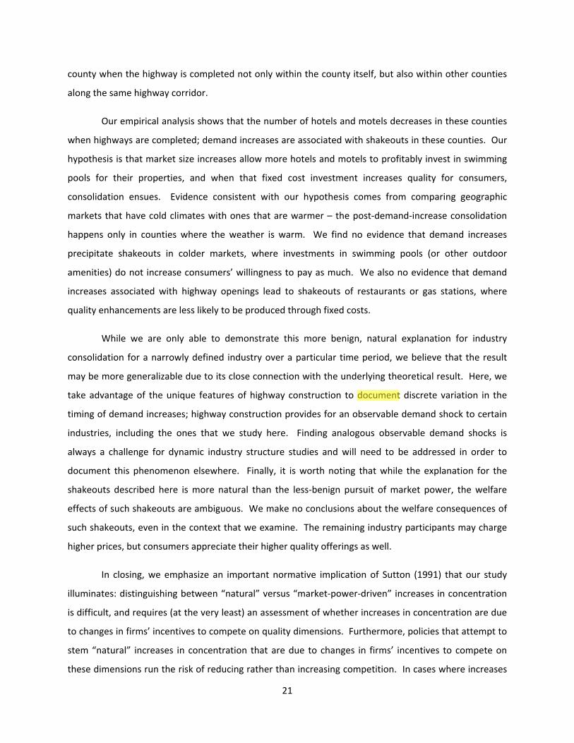
Figure 1.  Sutton (1991).  Increases in Market Size Can Lead to Shakeouts. 

The shaded area in the left panel of this Figure illustrates feasible equilibrium outcomes in the case of 

“exogenous sunk costs;” as market size increases, fragmented outcomes (i.e., where N is high) become 

feasible.  The shaded area in the right panel of this Figure illustrates feasible equilibrium outcomes in 

the case of “endogenous sunk costs;” here fragmented outcomes do not become possible as market size 

increases, and the equilibrium number of firms converges to a finite level.  The dashed lines depict 

possible relationships between market size and the number of firms.  The right panel illustrates that, 

under certain conditions, after some threshold where firms begin to compete on quality, the number of 

firms can decrease as market size increases. 

   

N

Market Size

Exogenous Sunk Costs

N

Market Size

Endogenous Sunk Costs

Increases in Market Size Create Entry Opportunities, Fragmentation Feasible

Increases in Market Size Initiate Non‐PriceCompetition, Shakeouts Possible

26  

 

 

Figure 2.  Hotel/Motel Employment, and the Number and Size of Hotels/Motels.  1964‐1992. 

   

0

200,000

400,000

600,000

800,000

1,000,000

1,200,000

1,400,000

1,600,000

Source: County Business Patterns, various years.

Hotel/Motel Employment, 1964‐1992

27  

 

 

Figure 3.  Establishment Shares of Hotels/Motels, by Number of Guestrooms.  1963, 1982. 

   

28  

 

 

Table 1.  Sources of Revenues, Recreational Facilities.  Hotels and Motels, various years. 

   

Sources of Revenues: Hotels and Motels

Food and Food and Bev/

Rooms Beverage Other Rooms

Hotels and Motels

1963 61% 34% 5% 0.56

1982 59% 26% 15% 0.44

Motels Only

1963 75% 22% 3% 0.29

1982 78% 19% 4% 0.24

Source: Census of Services, 1963, 1982.

"Motels" includes "motels" and "motor hotels" in 1963, and "motels," "motor hotels," and "tourist courts" in 1982.

1963 includes only hotels with 25 or more guestrooms and motels with 10 or more guestrooms; these hotels/motels

made up over 97% of industry revenues.

Recreational Facilities: Hotels and Motels

Share With….

Any Recreational Swimming  Private Pool or

Facillity Pool Beach Beach

Hotels and Motels

1963 30% 23% 5%

1967 37% 32% 7%

1972 51%

Motels Only

1963 32% 28% 4%

1982 43% 38% 6%

1972 55%

Source: Census of Services, 1963, 1967, 1972.

"Recreational Facility" includes swimming pool, boating, private beach, golf course, tennis court, horseback

riding, and skiing.

"Motels" includes "Motels" and "Motor Hotels."

29  

 

Figure 4.  Share of Hotels/Motels With Pool or Beach, by Average State Temperature.  1963, 1972. 

 

Figure 5.  Chain Share of Motel Revenues: 1967, 1977   

30  

 

 

Figure 6.  Two‐Digit Interstate Highway Construction, 1960‐1982. 

   

31  

 

 

 

Figure 7.  Sample Counties. 

This map depicts the 227 counties in our sample.  Warmer counties are indicated by red; cooler counties 

are indicated by blue. 

   

32  

 

 

Figure 8.  Average Employment, Sample Counties.  1964‐1992. 

 

0

100

200

300

400

500

600

700

1964 1966 1968 1970 1972 1974 1976 1978 1980 1982 1984 1986 1988 1990 1992

Hotel/Motel  Em

ploym

ent

Year

Average Hotel/Motel Employment, Sample Counties

33  

 

 

Figure 9.  Average Number of Hotels/Motels, Sample Counties.  1964‐1992. 

   

0

5

10

15

20

25

30

1964 1966 1968 1970 1972 1974 1976 1978 1980 1982 1984 1986 1988 1990 1992

Number of Hotels/M

otels

Year

Average Number of Hotels/Motels, Sample Counties

34  

 

 

Figure 10.  Average Number of Hotels/Motels Per 1000 County Employment, Sample Counties.  1964‐

1992. 

0

0.5

1

1.5

2

2.5

3

1964 1966 1968 1970 1972 1974 1976 1978 1980 1982 1984 1986 1988 1990 1992

Hotels/M

otels per 1000 Employm

ent

Year

Average Number of Hotels/Motels Per 1000 County Employment, Sample Counties

35  

 

 

Figure 11.  Interstate Highway Construction, Sample Counties.   

36  

 

 

Table 2

Regressions of County Hotel Employment on Corridor and County Highway Openings

Dependent Variable: ln(County Hotel Employment)

Sh(Corridor) 0.084 0.108

(0.028) (0.035)

Sh(County) ‐0.029

(0.026)

Sh (Corridor)*Dum(Corridor Construction in County) 0.090

(0.038)

Sh (Corridor)*Dum(All Corridor Construction Out of County) 0.214

     *Dum(No Construction Yet in County) (0.075)

Sh (Corridor)*Dum(All Corridor Construction Out of County) 0.077

     *Dum(County Partially Complete) (0.035)

Sh (Corridor)*Dum(All Corridor Construction Out of County) 0.095

     *Dum(County Fully Complete) (0.028)

AR Term 0.710 0.710 0.709

(0.011) (0.011) (0.011)

These results are from county‐level AR specifications that relate county hotel employment to Interstate Highway openings.

The specifications also include county and year fixed effects (not reported).

These results use all counties with non‐missing reports for number of firms/establishments from 1964‐1992, N=227.

Standard errors are in parentheses; bold indicates that the estimate is statistically significantly different zero using a test of size 0.05.

37  

 

Table 3

Regressions of Number and Size of Hotels on Corridor Completion

Dependent Variable: ln(Hotels/(County Employment*1000))

Sh(Corridor) ‐0.068 ‐0.048

(0.017) (0.021)

Sh(County) ‐0.024

(0.015)

Sh (Corridor)*Dum(Corridor Construction in County) ‐0.067

(0.023)

Sh (Corridor)*Dum(All Corridor Construction Out of County) ‐0.043

     *Dum(No Construction Yet in County) (0.045)

Sh (Corridor)*Dum(All Corridor Construction Out of County) ‐0.084

     *Dum(County Partially Complete) (0.021)

Sh (Corridor)*Dum(All Corridor Construction Out of County) ‐0.064

     *Dum(County Fully Complete) (0.017)

AR Term 0.774 0.772 0.774

(0.011) (0.011) (0.011)

Dependent Variable: ln(Employment/Hotel)

Sh(Corridor) 0.112 0.113

(0.028) (0.035)

Sh(County) ‐0.002

(0.026)

Sh (Corridor)*Dum(Corridor Construction in County) 0.110

(0.038)

Sh (Corridor)*Dum(All Corridor Construction Out of County) 0.186

     *Dum(No Construction Yet in County) (0.074)

Sh (Corridor)*Dum(All Corridor Construction Out of County) 0.101

     *Dum(County Partially Complete) (0.034)

Sh (Corridor)*Dum(All Corridor Construction Out of County) 0.118

     *Dum(County Fully Complete) (0.029)

AR Term 0.631 0.631 0.630

(0.013) (0.013) (0.013)

"Hotels" are Census reporting units.  Before 1974 this equals the number of firms (with positive employment)

operating hotels in the county.  Starting in 1973 this equals the number of hotels (with positive employment).

The specifications also include county and year fixed effects (not reported).  We also allow the autoregressive

coefficients to differ in year 1974 to accommodate the Census' change in reporting units between 1973 and 1974.

These results use all counties with non‐missing reports for number of firms/establishments from 1964‐1992, N=227.

Standard errors are in parentheses; bold indicates that the estimate is statistically significantly different zero using a test of size 0.05.

38  

   

   

Table 4

Regressions of Number of Hotels by Size Category on Corridor Highway OpeningsBy Status of Construction in the County

Dependent Variable V. Small Hotels Small Hotels Med. Hotels Large Hotels V. Small Hotels Small Hotels Med. Hotels Large Hotels

AR Term 0.744 0.444 0.510 0.734 0.744 0.443 0.508 0.733

(0.008) (0.011) (0.011) (0.009) (0.008) (0.011) (0.011) (0.009)

Sh(Corridor) ‐0.812 ‐0.063 0.169 0.568

(0.272) (0.153) (0.147) (0.135)

Sh (Corridor)*Dum(Corridor Construction in County) ‐1.029 0.213 0.074 0.643

(0.365) (0.205) (0.197) (0.181)

Sh (Corridor)*Dum(All Corridor Construction Out of County) ‐1.518 0.442 0.378 1.041

     *Dum(No Construction Yet in County) (0.681) (0.383) (0.369) (0.339)

Sh (Corridor)*Dum(All Corridor Construction Out of County) ‐0.805 0.057 0.023 0.724

     *Dum(County Partially Complete) (0.334) (0.188) (0.181) (0.167)

Sh (Corridor)*Dum(All Corridor Construction Out of County) ‐0.870 ‐0.030 0.195 0.592

     *Dum(County Fully Complete) (0.276) (0.155) (0.149) (0.137)

These results are from county‐level VAR specifications that relate the number of hotels in different size categories to Interstate Highway openings.

The specifications also include county and year fixed effects (not reported).

These results use all counties with non‐missing reports for number of firms/establishments from 1964‐1992, N=226.

Standard errors are in parentheses; bold indicates that the estimate is statistically significantly different zero using a test of size 0.05.

Very Small Hotels: 1‐3 employees (before 1974), 1‐4 employees (1974 on).

Small Hotels: 4‐7 employees (before 1974), 5‐9 employees (1974 on).

Medium Hotels: 8‐19 employees (before 1974), 10‐19 employees (1974 on).

Large Hotels: 20 or more employees.

39  

   

 

   

Table 5

Interaction Effects with Temperature ‐‐ Hotels

ln(County Hotel ln(Hotels/ ln(Employees/

Dependent Variable: Employment) County Emp*1000)) Hotel)

Sh(Corridor) 0.079 ‐0.048 0.089

(0.029) (0.017) (0.029)

Sh(Corridor)*Temperature 0.001 ‐0.005 0.004

(0.002) (0.001) (0.002)

Dependent Variable: V. Small Hotels Small Hotels Med. Hotels Large Hotels

Sh(Corridor) ‐0.551 0.030 0.301 0.334

(0.281) (0.159) (0.152) (0.139)

Sh(Corridor)*Temperature ‐0.060 ‐0.021 ‐0.030 0.054

(0.017) (0.010) (0.009) (0.008)

"Hotels" are Census reporting units.  Before 1974 this equals the number of firms (with positive employment)

operating hotels in the county.  Starting in 1973 this equals the number of hotels (with positive employment).

The specifications also include county and year fixed effects (not reported).  We also allow the autoregressive

coefficients to differ in year 1974 to accommodate the Census' change in reporting units between 1973 and 1974.

These results use all counties with non‐missing reports for number of firms/establishments from 1964‐1992, N=227.

Standard errors are in parentheses; bold indicates that the estimate is statistically significantly different zero using a test of size 0.05.

Very Small Hotels: 1‐3 employees (before 1974), 1‐4 employees (1974 on).

Small Hotels: 4‐7 employees (before 1974), 5‐9 employees (1974 on).

Medium Hotels: 8‐19 employees (before 1974), 10‐19 employees (1974 on).

Large Hotels: 20 or more employees.

 

 

 

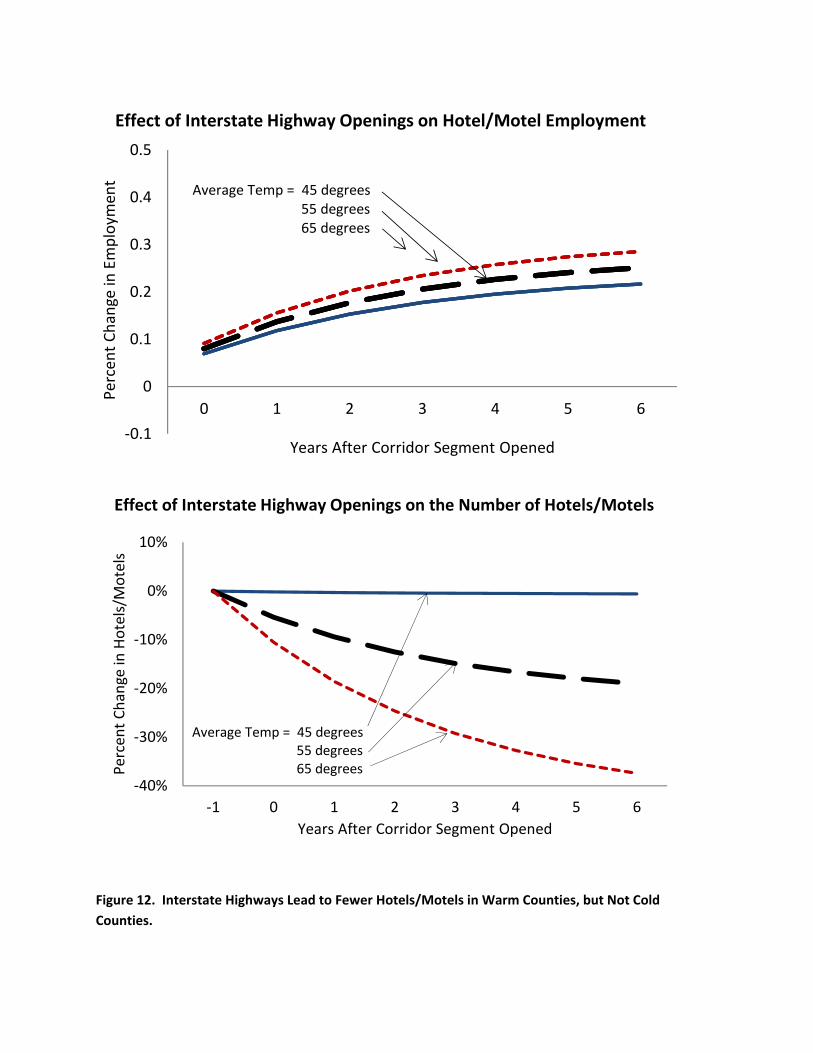
Figure 12.  Interstate Highways Lead to Fewer Hotels/Motels in Warm Counties, but Not Cold 

Counties. 

‐0.1

0

0.1

0.2

0.3

0.4

0.5

0 1 2 3 4 5 6

Percent Change in

 Employm

ent

Years After Corridor Segment Opened

Average Temp = 45 degrees55 degrees65 degrees

Effect of Interstate Highway Openings on Hotel/Motel Employment

‐40%

‐30%

‐20%

‐10%

0%

10%

‐1 0 1 2 3 4 5 6

Percent Change in

 Hotels/M

otels

Years After Corridor Segment Opened

Effect of Interstate Highway Openings on the Number of Hotels/Motels

Average Temp = 45 degrees55 degrees65 degrees

  

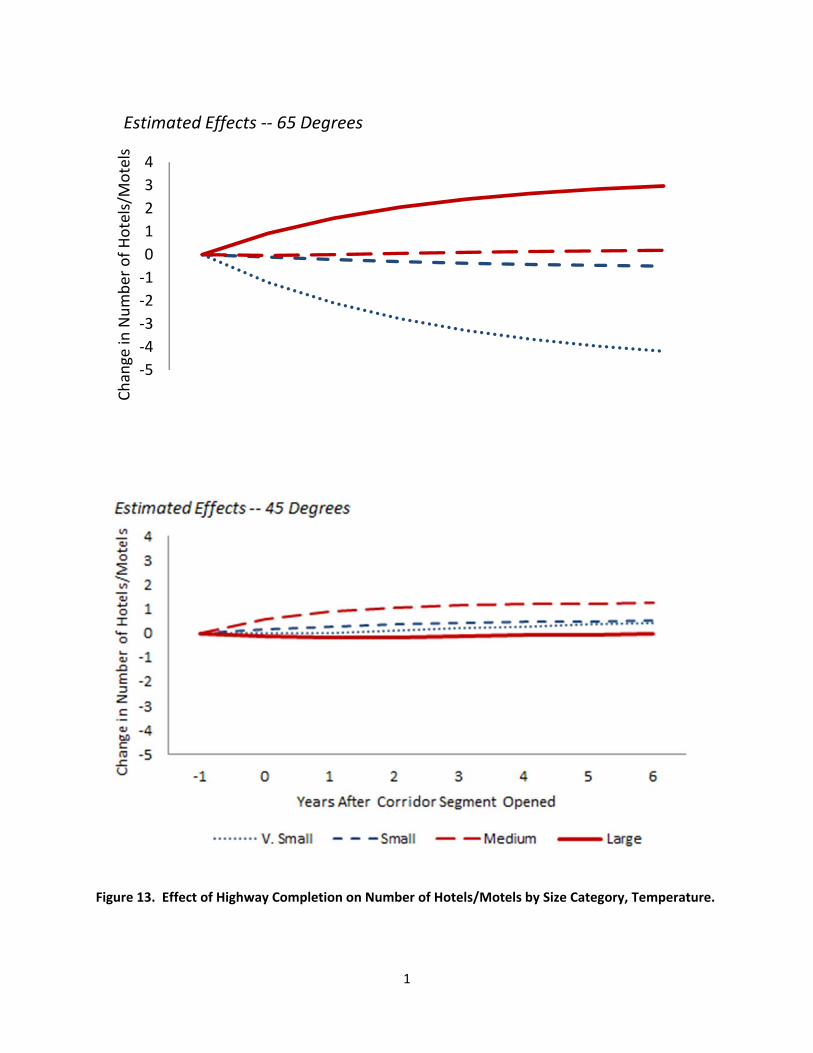
1

 

 

Figure 13.  Effect of Highway Completion on Number of Hotels/Motels by Size Category, Temperature.

‐5

‐4

‐3

‐2

‐1

0

1

2

3

4

Change in

 Number of Hotels/M

otels

Estimated Effects ‐‐ 65 Degrees

  

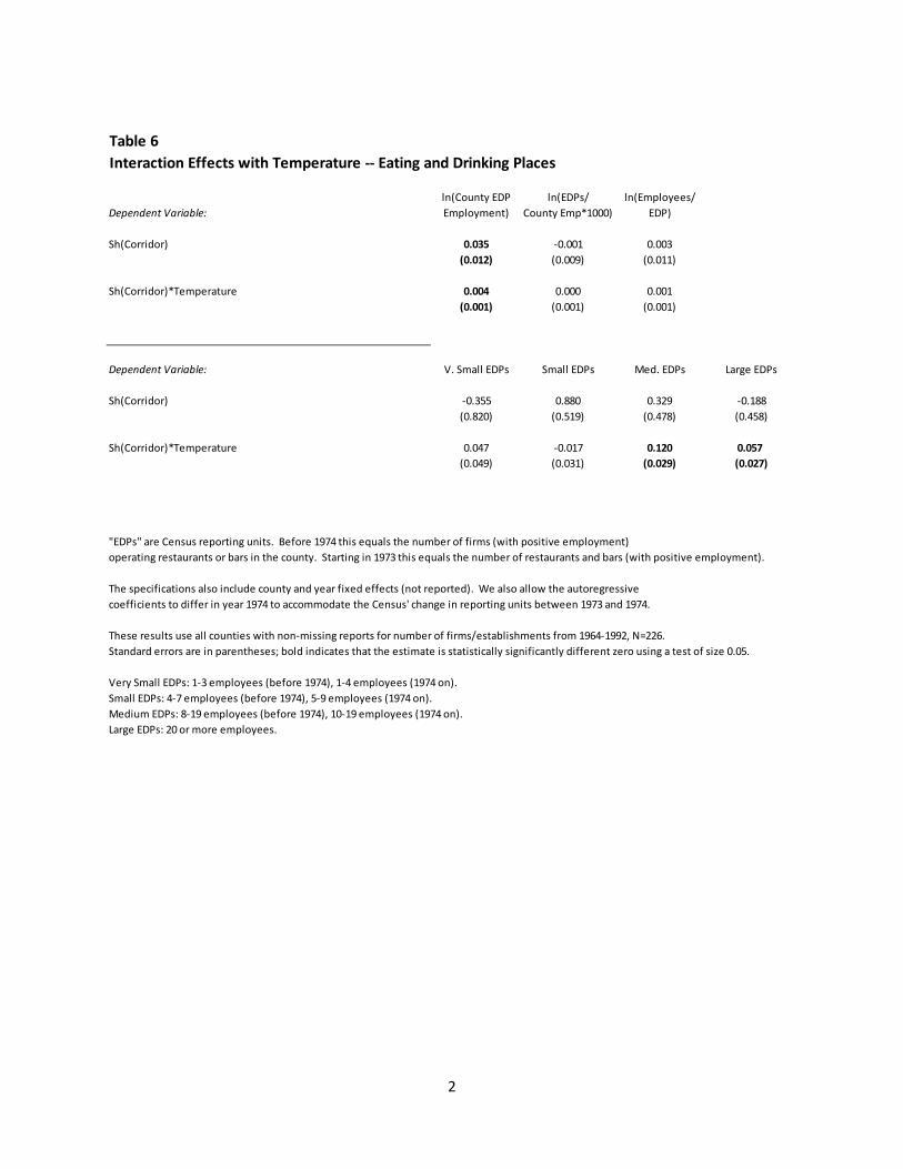
2

 

 

   

Table 6

Interaction Effects with Temperature ‐‐ Eating and Drinking Places

ln(County EDP ln(EDPs/ ln(Employees/

Dependent Variable: Employment) County Emp*1000)) EDP)

Sh(Corridor) 0.035 ‐0.001 0.003

(0.012) (0.009) (0.011)

Sh(Corridor)*Temperature 0.004 0.000 0.001

(0.001) (0.001) (0.001)

Dependent Variable: V. Small EDPs Small EDPs Med. EDPs Large EDPs

Sh(Corridor) ‐0.355 0.880 0.329 ‐0.188

(0.820) (0.519) (0.478) (0.458)

Sh(Corridor)*Temperature 0.047 ‐0.017 0.120 0.057

(0.049) (0.031) (0.029) (0.027)

"EDPs" are Census reporting units.  Before 1974 this equals the number of firms (with positive employment)

operating restaurants or bars in the county.  Starting in 1973 this equals the number of restaurants and bars (with positive employment).

The specifications also include county and year fixed effects (not reported).  We also allow the autoregressive

coefficients to differ in year 1974 to accommodate the Census' change in reporting units between 1973 and 1974.

These results use all counties with non‐missing reports for number of firms/establishments from 1964‐1992, N=226.

Standard errors are in parentheses; bold indicates that the estimate is statistically significantly different zero using a test of size 0.05.

Very Small EDPs: 1‐3 employees (before 1974), 1‐4 employees (1974 on).

Small EDPs: 4‐7 employees (before 1974), 5‐9 employees (1974 on).

Medium EDPs: 8‐19 employees (before 1974), 10‐19 employees (1974 on).

Large EDPs: 20 or more employees.

  

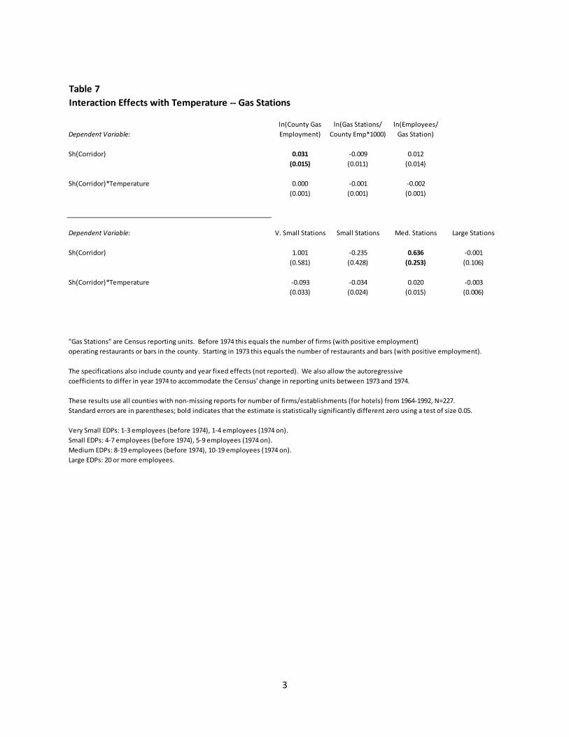
3

 

 

   

Table 7

Interaction Effects with Temperature ‐‐ Gas Stations

ln(County Gas ln(Gas Stations/ ln(Employees/

Dependent Variable: Employment) County Emp*1000)) Gas Station)

Sh(Corridor) 0.031 ‐0.009 0.012

(0.015) (0.011) (0.014)

Sh(Corridor)*Temperature 0.000 ‐0.001 ‐0.002

(0.001) (0.001) (0.001)

Dependent Variable: V. Small Stations Small Stations Med. Stations Large Stations

Sh(Corridor) 1.001 ‐0.235 0.636 ‐0.001

(0.581) (0.428) (0.253) (0.106)

Sh(Corridor)*Temperature ‐0.093 ‐0.034 0.020 ‐0.003

(0.033) (0.024) (0.015) (0.006)

"Gas Stations" are Census reporting units.  Before 1974 this equals the number of firms (with positive employment)

operating restaurants or bars in the county.  Starting in 1973 this equals the number of restaurants and bars (with positive employment).

The specifications also include county and year fixed effects (not reported).  We also allow the autoregressive

coefficients to differ in year 1974 to accommodate the Census' change in reporting units between 1973 and 1974.

These results use all counties with non‐missing reports for number of firms/establishments (for hotels) from 1964‐1992, N=227.

Standard errors are in parentheses; bold indicates that the estimate is statistically significantly different zero using a test of size 0.05.

Very Small EDPs: 1‐3 employees (before 1974), 1‐4 employees (1974 on).

Small EDPs: 4‐7 employees (before 1974), 5‐9 employees (1974 on).

Medium EDPs: 8‐19 employees (before 1974), 10‐19 employees (1974 on).

Large EDPs: 20 or more employees.

  

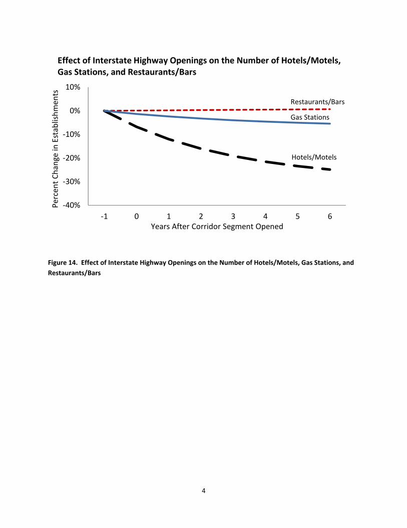
4

 

 

Figure 14.  Effect of Interstate Highway Openings on the Number of Hotels/Motels, Gas Stations, and 

Restaurants/Bars 

‐40%

‐30%

‐20%

‐10%

0%

10%

‐1 0 1 2 3 4 5 6

Percent Change in

 Establishmen

ts

Years After Corridor Segment Opened

Effect of Interstate Highway Openings on the Number of Hotels/Motels,Gas Stations, and Restaurants/Bars

Restaurants/Bars

Hotels/Motels

Gas Stations