Heterogeneous Firms, Quality and Trade�

Alexis Antoniades

Draft

Aug 11, 2008

Abstract

We present a model of quality choice in a world of heterogeneous �rms and non-constant markups. In

equilibrium, some �rms exit the market, others produce output but choose no quality upgrades, and the

most productive �rms produce both output and quality upgrades. For these �rms, the more productive

they are, the more quality they choose.

In line with recent empirical �ndings, the model shows that prices can increase in productivity,

that developing countries have an incentive to export more quality goods to developed countries than

developing, and that competition in endogenous sunk costs industries does not have to lead to market

fragmentation. The model also generates the Linder hypothesis from the supply side, and the Balassa-

Samuelson e¤ect. Finally, trade partner characteristics do a¤ect the level of competition in the host

country when quality choice is taken into consideration.

Keywords: Intra-industry trade, �rm heterogeneity, qualilty choice, markups

�aa658@georgetown.edu. I would like to thank Don Davis, James Harrigan, Amit Khandelwal, Eric Verhoogen, David

Weinstein, and participants at the International Trade Colloquium at Columbia University for helpful comments and suggestions.

1

Recently, the role of quality has received a lot of attention in international trade. Bernard et al. (2006)

document that capital and skill abundant countries use their endowment advantage to produce vertically

superior varieties that have higher prices. Similarly, Hallak (2006) shows that the quality of goods produced

and consumed varies systematically with the income level. Baldwin and Harrigan (2007) �nd that export

unit-prices increase with distance. The authors point out that leading trade models can only account for

this price pattern if quality is introduced. Verhoogen (2008) shows that the rising wage inequality gap

in developing countries can be explained in a model where �rms export high quality goods to developed

countries and hence, they demand high skill labor. Finally, Hummels and Klenow (2002) �nd that in rich

countries, a large portion of the increase in exports occurs through quality upgrades.

Three main observations come from analyzing the studies above. First, quality is essential in trying to

understand the empirical �ndings. Second, in order to account for these �ndings, several ad-hoc assumptions

are made. For instance, it is assumed that consumers in rich countries have higher preferences for quality

than consumers in poor countries (Murphy and Schleifer [1997], Choi et al[2006]). It is also assumed that

developing countries export goods of higher quality to developed countries than developing (Verhoogen

[2008]), or that the level of quality increases with productivity (Baldwin and Harrigan [2007]). Third, in

isolation, none of the assumptions above can account for the entire set of stylized facts.

This paper presents a model of quality choice with heterogeneous �rms and non-constant markups that

matches the stylized facts mentioned, but also generates endogenously several of the assumptions discussed

above. The model is based on Melitz and Ottaviano (2007) model of heterogeneous �rms with linear demand

functions. As in Melitz and Ottaviano (MO), �rms pay a �xed cost to be able to draw a marginal cost

(productivity) parameter from a distribution. Firms with high marginal costs (low productivity) exit.

Firms with lower marginal costs stay in the market and produce heterogeneous goods. The MO framework

is augmented to include quality. On the demand side, the consumers like quality and hence, a new utility

function is presented to account for this fact. On the supply side, the �rms not only choose whether to

produce or not, but they also choose whether to undertake quality upgrades for their products. If all �rms

choose not to upgrade quality, then this model collapses to the MO framework. In this sense, our model

nests that of MO. A �rm has incentive to invest in quality upgrade since consumers like quality. However,

2

quality comes at a cost. If a �rm chooses to produce quality, it needs to pay an extra �xed cost (with

respect to quantity) that increases with the level of quality upgrade it chooses to undertake. Any choice of

quality upgrade does not a¤ect the marginal cost of each unit produced, but it a¤ects the markup a �rm

charges for that unit and therefore, its price. The choice of quality upgrade is continuous and non-negative.

Several interesting features come out of the model. First, at equilibrium there are three types of �rms.

Some �rms draw high marginal costs and choose to exit the market. Others, produce output but choose

not to undertake any quality upgrades. For these �rms, their productivity is high enough to enable them to

produce output, but not high enough to enable them to recover the �xed cost of innovation. And �nally,

there are �rms that produce both output and quality upgrades. These are the most productive �rms in the

market.

Second, for the set of �rms that choose quality upgrade, the higher their productivity is (lower marginal

cost), the more quality upgrade they choose. As �rms get more productive, it becomes easier for them to

recover the �xed cost of innovation. More innovation raises quality and more quality raises the consumers�

willingness to pay. Hence, the model can generate endogenously the �rst assumption made by Baldwin and

Harrigan (2007) that quality increases in productivity1 . This point is also made by Johnson (2007) in a

similar paper that also endogenizes quality choice in a CES framework.

Third, if the elasticity of markups with respect to quality choice is high, prices increase in productivity

even though marginal costs fall. In standard heterogeneous �rms models (eg. Melitz [2003], Melitz and

Ottaviano [2007]) the opposite is true. The more productive a �rm is, the lower its marginal cost and

the lower price it charges. This is because �rms set prices as markups over marginal cost, and markups are

assumed to be constant. Baldwin and Harrigan study how US export unit prices vary with export destination

distance and �nd that unit prices increase in distance. They argue that their �nding is consistent with models

where prices increase in productivity. Here, a �rm with high productivity will have lower marginal costs.

However, it will also have an incentive to produce more quality and raise the markup of its product. If

the increase in markup is su¢ ciently large to o¤set the drop in marginal cost, then prices can rise with

productivity.

1The second assumption in their paper is that quality raises the marginal cost.

3

Fourth, the model predicts that the share of quality goods produced and consumed in developed/large

countries will be higher than in developing/small countries. As the size of the country gets larger, or the

country becomes more developed (ability to innovate increases), more �rms undertake quality upgrades, and

the level of quality upgrade undertaken by each �rm increases. Intuitively, it is easier to recover the �xed

cost of innovation when the market size is large or when the cost of innovation is low. Therefore, in rich

and/or large countries, the model predicts a higher share of quality goods produced and consumed. This

prediction is known as the Linder hypothesis. In past work, the explanation of the Linder hypothesis came

from the demand side, by assuming that consumers in rich countries have higher preferences for quality. In

contrast, here we o¤er a supply-side explanation of the Linder hypothesis.

Fifth, trade with developed countries results in more quality upgrade. Verhoogen (2007) documents that

Mexican �rms have an incentive to export more quality goods when they trade with the US. We show that

trade with developed countries encourages �rms to upgrade quality, both for the export market and the

domestic. That is, not only do Mexican �rms export more quality goods when they trade with the US, but

they also upgrade the quality of the goods produced for the domestic market.

Sixth, more competition does not necessarily result in market fragmentation as most trade models predict.

Sutton (1989, 1991) argues that in an endogenous sunk cost industry, more competition encourages the

dominant �rms to di¤erentiate their products, either vertically or horizontally, by paying a higher sunk cost.

As the products become more di¤erentiated, the consumers�willingness to pay increases along with the �rms�

market share. Sutton�s insight is re�ected in this model. As the market size expands, competition increases.

However, the propensity to upgrade quality also increases as it becomes easier to recover the �xed cost of

innovation. For the least productive �rms the former of the two e¤ects is stronger resulting in �rms loosing

market share due to competition. For the most productive �rms, the latter of the two e¤ects is stronger.

These �rms choose to pay a higher sunk cost and di¤erentiate their products more as Sutton suggests2 .

Enough product di¤erentiation may actually increase their market share even if competition increases.

Seventh, the model generates the Balassa-Samuelson e¤ect. Trade with rich countries encourages the most

productive �rms to increase quality, and forces the least productive to lower quality. The most productive

2The model is also consistent with two other insights of Sutton, namely that there is a lower bound to quality and the

window of quality levels increases with trade liberalization (Sutton [2007]).

4

�rms raise quality because they now have access to a larger market and thus, recovering the �xed cost of

innovation is easier. However, �rms that are not very productive have to cut back on quality and lower their

markups because this extra competition reduces their market share. Since the least productive �rms are the

ones that produce the non-traded goods, the price of a basket of non-traded goods falls, while the price of a

basket of traded goods rises, for these goods now have higher quality relative to the non-traded goods.

Eighth, the model shows that trade partner characteristics do a¤ect domestic market competition and

the cost threshold between the �rms that produce and those that do not. Trade with large countries creates

more competition than trade with small countries does, and trade with developed countries induces more

quality upgrades than trade with developing.

In the benchmark version of the model, we assume that quality raises the endogenous �xed cost but not

the marginal cost of production. Usually, in quality models, the higher the level of quality choice is, the

higher the marginal cost, while markups remain constant. Given that the existing literature has provided

very important insights on how quality a¤ects prices and competition through altering marginal costs, we

decide to focus our attention on the link between quality choice and markups. That is, we do not reject

the fact that adding quality raises marginal costs. Rather, we try to augment our understanding of the

dynamics of quality choice on trade through the impact it has on markups. Exploring this channel is precisely

the objective of the paper. As discussed above, once we endogenize quality choice and markups, a lot of

interesting dynamics and predictions come out of the model. In an (unpublished) appendix we solve the

model by relaxing this assumption and show that the main predictions of the model are not altered.

In earlier versions of this work we worked with CES preferences3 . In the surface, both models are similar.

Both models predict that quality choice increases in productivity. However, there are four substantial

di¤erences. First, in a CES framework the level of quality choice does not a¤ect markups, so we cannot

exploit the trade-o¤ between the cost of adding quality and the gain from raising markups. Second, if prices

do increase in productivity, the CES framework can only attribute this to rising MC. However, in this

paper, we show that prices can also rise due to an increases in markups. Third, the choice of quality in

the CES framework does not depend on domestic (and foreign) country characteristics (such as size and

3Robert Johnson (2007) develops a CES version in more detail.

5

ability to innovate), whereas in the paper presented below we show that quality does depend on country

characteristics. Therefore, under CES, the level of quality choice will not be larger in developed, rich and/or

large countries, in contrast to evidence from recent work by Khandelwal (2008) and Schott (2004). As a

result, the CES model cannot generate the Linder hypothesis. Also, the Verhoogen (2008) insight that trade

with developed countries encourages �rms to produce and export high quality goods cannot be explained

in the CES model without assuming that consumer in rich countries have stronger preference for quality.

Furthermore, with CES preferences more competition results in market fragmentation, in contrast to the

Sutton insight. Fourth, the CES framework can only be solved for the symmetric case, whereas this model

can be solved for the asymmetric case (with the symmetric case being a special case).

The paper proceeds as follows: Section 2 presents the closed economy version of the model. A reader

familiar to MO will observe that our model looks almost identical to MO. However, underneath there is a

much richer world. Consumers have di¤erent preferences and �rms not only choose price and quantity, but

they also choose quality. One important contribution of the model is that it describes this rich environment

without giving up simplicity or tractability. Simplicity helps the reader obtain the intuition behind the

model, and tractability allows one to extend this model is several meaningful directions that we discuss at

the end. Section 3 presents a two-country version of the model that can be used to study how openness and

trade policy a¤ect equilibrium when quality choice is taken into consideration. Section 4 parameterizes a

version of the model and obtains expressions for aggregate variables such as average cost, price, markups and

quality. Section 5 analyzes the model when parameters change or the country trades. Section 6 concludes

this work.

1 One-Country Model

1.1 Consumers

The preferences for a typical consumer are given by

U = qco+�

Zi2

qci di+�

Zi2

zidi�1

2

Zi2

(qci )2di� 1

2

Zi2

(zi)2di+

Zi2

(qci zi) di�1

2�

8<:Zi2

�qci �

1

2zi

�di

9=;2

(1)

6

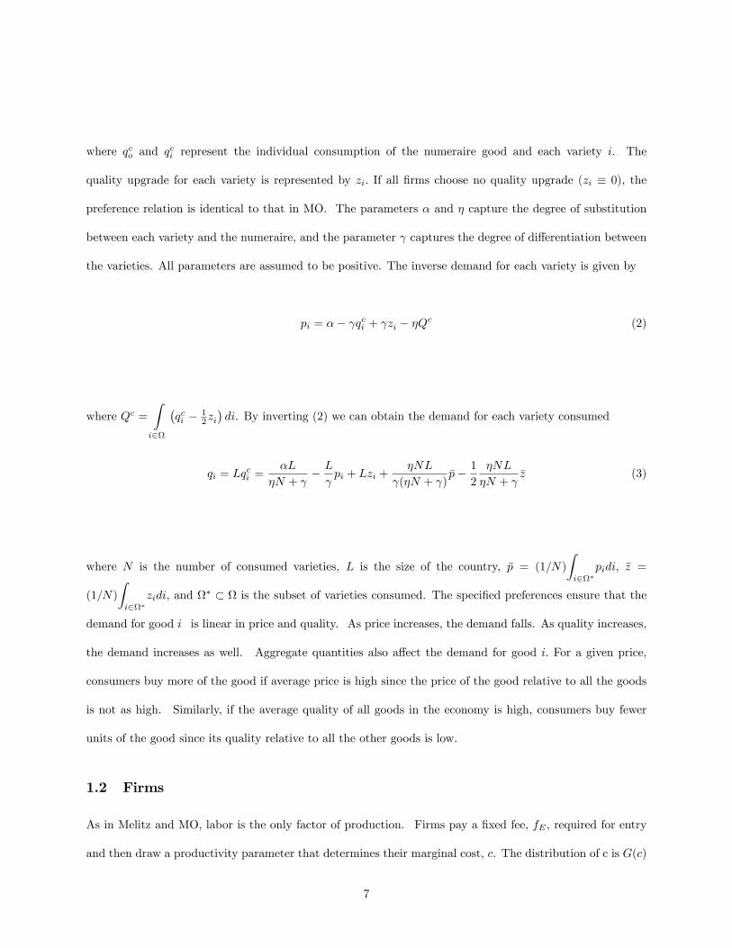
where qco and qci represent the individual consumption of the numeraire good and each variety i. The

quality upgrade for each variety is represented by zi: If all �rms choose no quality upgrade (zi � 0), the

preference relation is identical to that in MO. The parameters � and � capture the degree of substitution

between each variety and the numeraire, and the parameter captures the degree of di¤erentiation between

the varieties. All parameters are assumed to be positive. The inverse demand for each variety is given by

pi = �� qci + zi � �Qc (2)

where Qc =Zi2

�qci � 1

2zi�di. By inverting (2) we can obtain the demand for each variety consumed

qi = Lqci =

�L

�N + � L pi + Lzi +

�NL

(�N + )�p� 1

2

�NL

�N + �z (3)

where N is the number of consumed varieties, L is the size of the country, �p = (1=N)

Zi2�

pidi; �z =

(1=N)

Zi2�

zidi, and � � is the subset of varieties consumed. The speci�ed preferences ensure that the

demand for good i is linear in price and quality. As price increases, the demand falls. As quality increases,

the demand increases as well. Aggregate quantities also a¤ect the demand for good i: For a given price,

consumers buy more of the good if average price is high since the price of the good relative to all the goods

is not as high. Similarly, if the average quality of all goods in the economy is high, consumers buy fewer

units of the good since its quality relative to all the other goods is low.

1.2 Firms

As in Melitz and MO, labor is the only factor of production. Firms pay a �xed fee, fE , required for entry

and then draw a productivity parameter that determines their marginal cost, c. The distribution of c is G(c)

7

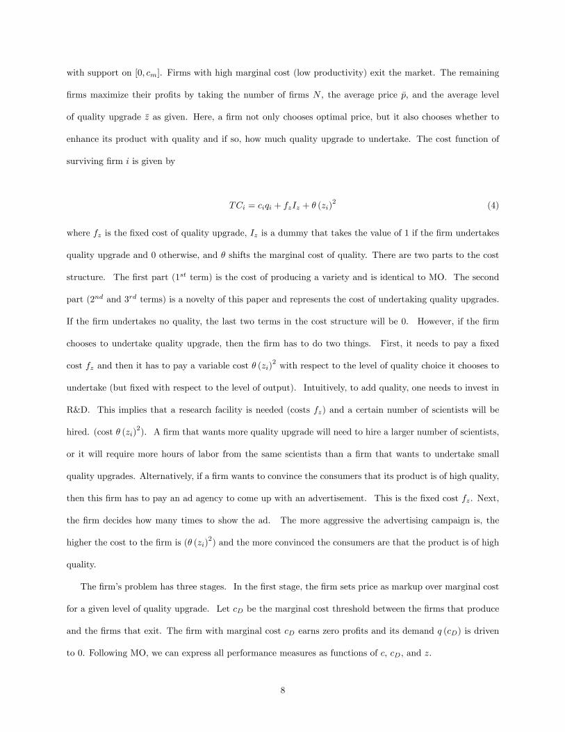
with support on [0; cm]. Firms with high marginal cost (low productivity) exit the market. The remaining

�rms maximize their pro�ts by taking the number of �rms N , the average price �p, and the average level

of quality upgrade �z as given. Here, a �rm not only chooses optimal price, but it also chooses whether to

enhance its product with quality and if so, how much quality upgrade to undertake. The cost function of

surviving �rm i is given by

TCi = ciqi + fzIz + � (zi)2 (4)

where fz is the �xed cost of quality upgrade, Iz is a dummy that takes the value of 1 if the �rm undertakes

quality upgrade and 0 otherwise, and � shifts the marginal cost of quality. There are two parts to the cost

structure. The �rst part (1st term) is the cost of producing a variety and is identical to MO. The second

part (2nd and 3rd terms) is a novelty of this paper and represents the cost of undertaking quality upgrades.

If the �rm undertakes no quality, the last two terms in the cost structure will be 0. However, if the �rm

chooses to undertake quality upgrade, then the �rm has to do two things. First, it needs to pay a �xed

cost fz and then it has to pay a variable cost � (zi)2 with respect to the level of quality choice it chooses to

undertake (but �xed with respect to the level of output). Intuitively, to add quality, one needs to invest in

R&D. This implies that a research facility is needed (costs fz) and a certain number of scientists will be

hired. (cost � (zi)2). A �rm that wants more quality upgrade will need to hire a larger number of scientists,

or it will require more hours of labor from the same scientists than a �rm that wants to undertake small

quality upgrades. Alternatively, if a �rm wants to convince the consumers that its product is of high quality,

then this �rm has to pay an ad agency to come up with an advertisement. This is the �xed cost fz. Next,

the �rm decides how many times to show the ad. The more aggressive the advertising campaign is, the

higher the cost to the �rm is (� (zi)2) and the more convinced the consumers are that the product is of high

quality.

The �rm�s problem has three stages. In the �rst stage, the �rm sets price as markup over marginal cost

for a given level of quality upgrade. Let cD be the marginal cost threshold between the �rms that produce

and the �rms that exit. The �rm with marginal cost cD earns zero pro�ts and its demand q (cD) is driven

to 0. Following MO, we can express all performance measures as functions of c, cD, and z:

8

p(c; z) =1

2[cD + c] +

2z (5a)

q(c; z) =L

2 [cD � c] +

L

2z (5b)

r(c; z) =L

4

h(cD)

2 � c2i+L

2zcD +

L

4z2 (5c)

�(c; z) =L

4 [cD � c]2 +

L

2z [cD � c] +

L

4z2 � fzIz � �z2 (5d)

The �rst proposition in the paper relates the amount of quality upgrade a �rm chooses given its marginal

cost and the threshold cost cD for the economy.

Proposition 1 The amount of quality upgrade a �rm chooses is increasing in the productivity of the �rm,

in the ability to innovate (low �), in the degree of product di¤erentiation ( )and in the size of the economy

(L).

Proof. In the second stage, the �rm chooses the level of quality that maximizes the pro�t function above.

Taking the derivative of �(c; z) with respect to z yields the optimal level of quality upgrade:

z� = � [cD � c] (5f)

where � = L=(4� � L ).

Since we are interested in situations where quality upgrade is positive, we assume that � > L =4. The

parameter �� is country (or industry) speci�c and is the slope of quality with respect to cost. The higher

the cost of a �rm is, the lower the level of quality it chooses. The further away a �rm is from the cost

threshold cD, the more quality upgrade it chooses.

The performance measures can now be re-written as functions of c; and cD:

9

p(c; z�) =1

2[cD + c] +

�

2[cD � c] Iz (7a)

q(c; z�) =L

2 [cD � c] +

L �

2[cD � c] Iz (7b)

r(c; z�) =L

4

h(cD)

2 � c2i+L�

2[cD � c] cDIz +

L �2

4[cD � c]2 Iz (7c)

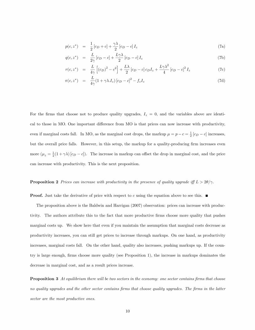
�(c; z�) =L

4 (1 + �:Iz) [cD � c]2 � fzIz (7d)

For the �rms that choose not to produce quality upgrades, Iz = 0, and the variables above are identi-

cal to those in MO. One important di¤erence from MO is that prices can now increase with productivity,

even if marginal costs fall. In MO, as the marginal cost drops, the markup � = p� c = 12 [cD � c] increases,

but the overall price falls. However, in this setup, the markup for a quality-producing �rm increases even

more (�z =12 (1 + �) [cD � c]). The increase in markup can o¤set the drop in marginal cost, and the price

can increase with productivity. This is the next proposition.

Proposition 2 Prices can increase with productivity in the presence of quality upgrade i¤ L > 2�= :

Proof. Just take the derivative of price with respect to c using the equation above to see this.

The proposition above is the Baldwin and Harrigan (2007) observation: prices can increase with produc-

tivity. The authors attribute this to the fact that more productive �rms choose more quality that pushes

marginal costs up. We show here that even if you maintain the assumption that marginal costs decrease as

productivity increases, you can still get prices to increase through markups. On one hand, as productivity

increases, marginal costs fall. On the other hand, quality also increases, pushing markups up. If the coun-

try is large enough, �rms choose more quality (see Proposition 1), the increase in markups dominates the

decrease in marginal cost, and as a result prices increase.

Proposition 3 At equilibrium there will be two sectors in the economy: one sector contains �rms that choose

no quality upgrades and the other sector contains �rms that choose quality upgrades. The �rms in the latter

sector are the most productive ones.

10

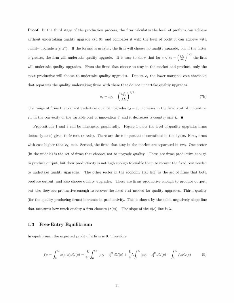
Proof. In the third stage of the production process, the �rm calculates the level of pro�t is can achieve

without undertaking quality upgrade �(c; 0), and compares it with the level of pro�t it can achieve with

quality upgrade �(c; z�). If the former is greater, the �rm will choose no quality upgrade, but if the latter

is greater, the �rm will undertake quality upgrade. It is easy to show that for c < cd ��4fz�L

�1=2the �rm

will undertake quality upgrades. From the �rms that choose to stay in the market and produce, only the

most productive will choose to undertake quality upgrades. Denote cz the lower marginal cost threshold

that separates the quality undertaking �rms with these that do not undertake quality upgrades.

cz = cD ��4fz�L

�1=2(7h)

The range of �rms that do not undertake quality upgrades cd � cz increases in the �xed cost of innovation

fz; in the convexity of the variable cost of innovation �, and it decreases is country size L.

Propositions 1 and 3 can be illustrated graphically. Figure 1 plots the level of quality upgrades �rms

choose (y-axis) given their cost (x-axis). There are three important observations in the �gure. First, �rms

with cost higher than cD exit. Second, the �rms that stay in the market are separated in two. One sector

(in the middle) is the set of �rms that chooses not to upgrade quality. These are �rms productive enough

to produce output, but their productivity is not high enough to enable them to recover the �xed cost needed

to undertake quality upgrades. The other sector in the economy (far left) is the set of �rms that both

produce output, and also choose quality upgrades. These are �rms productive enough to produce output,

but also they are productive enough to recover the �xed cost needed for quality upgrades. Third, quality

(for the quality producing �rms) increases in productivity. This is shown by the solid, negatively slope line

that measures how much quality a �rm chooses (z(c)). The slope of the z(c) line is �.

1.3 Free-Entry Equilibrium

In equilibrium, the expected pro�t of a �rm is 0. Therefore

fE =

Z cd

0

�(c; z)dG(c) =L

4

Z cD

0

[cD � c]2 dG(c) +L

4�

Z cz

0

[cD � c]2 dG(c)�Z cz

0

fzdG(c) (9)

11

The condition above determines the cuto¤ cost cD: The number of surviving �rms can be found from

(2). Set qi = 0; then

cD =1

�N + (� + �N �p� 1

2�N �z) (10)

It can be shown that

N =2

�

(a� cD)(cD � �c)

(11)

Readers familiar with the MO work will notice that our expression for the number of �rms is identical to

that in MO. This is not a mistake. The dynamics of quality choice on prices, competition, markups, etc

are summarized by the term cD. It is in the sense that we argue simplicity is not lost even though a much

richer framework is introduced.

2 Two-Country Model

2.1 Consumers

We now extend the closed economy model to a two-country setting. There is a home (H) and a foreign

(F ) country. Each country is endowed with LH and LF workers (consumers). For simplicity, assume that

consumers have identical preferences across the two countries and there is no labor mobility. As in the

closed-economy setting, the demand for good i in country l (l = fH;Fg) is given by

qli = Llqci =

�Ll

�N l + � L

l

pli + L

lzi +�N lLl

(�N l + )�pl � 1

2

�N lLl

�N l + �zl (12)

where pli and qli is the price of good i and quantity demanded in country l, respectively. Average price and

quality in country l are given by �pl and �zl. There are N l �rms selling in country l. These are both domestic

�rms and foreign exporters. A �rm does not discriminate in quality between domestic and foreign sales, but

it does discriminate in price. This is why quality does not have a country superscript by price does. Later

12

in the paper, we relax this assumption and allow �rms to set di¤erentiated levels of quality for the domestic

and the foreign markets.

2.2 Firms:

As in the closed economy setting, a �rm chooses whether to produce or not, and whether to install quality

upgrades. The �rm now has the option to export. There is cost to exporting, so not all �rms choose to

export. A �rm that exports sets two di¤erent prices, one for the domestic market and one for the foreign

market. The level of quality it chooses, however, is �xed. There is no di¤erence in the quality of a product

the �rm exports to the one it sells domestically. The delivery cost of a unit with cost c to country l is

� lc4 . Let pl(c) and ql(c) be the domestic level of the pro�t maximizing price and quantity, respectively. The

operating pro�t (ignores �xed costs and cost to quality upgrade) from domestic and foreign sales is given by

�lD(c; z) =�plD(c; z)� c

�qlD(c; z) (13a)

�lX(c; z) =�plX(c; z)� �hc

�qlX(c; z) (13b)

The pro�t maximizing prices and quantities must satisfy

qlD(c; z) =Ll

�plD(c; z)� c

�(14a)

qlX(c; z) =Lh

�plx(c; z)� �hc

�(14b)

The production cuto¤s are de�ned as

clD = sup��lD(c) > 0

= pl (15a)

clX = sup��lX(c) > 0

=ph

�h(15b)

4 In the appendix I present the solution of the model when a per-unit cost of export is impossed. That is, the cost of

delivering a unit with cost c to country l is now � l + c instead of � lc. Prof James Harrigan suggested this exercise.

13

We assumed here that the quality cost threshold is to the left of the export cost threshold. Combining the

cuto¤s conditions for the two countries, it is easy to show that chX = clD=�

l . The optimal price and quantity

for the domestic and the foreign market can now be expressed as functions of the cuto¤ cost thresholds.

plD(c; z) =1

2(clD + c) +

2z (16a)

plX(c; z) =�h

2(clX + c) +

2z (16b)

qlD(c; z) =Ll

2 (clD � c) +

Ll

2z (16c)

qlX(c; z) =Lh

2 �h(clX � c) +

Lh

2z (16d)

Given prices and quantities, operating pro�t of the �rm in each market is given by

�lD(c; z) =Ll

4 (clD � c)2 +

Ll

2z(clD � c) +

Ll

4z2 (17a)

�lx(c; z) =Lh

4 (�h)2(clX � c)2 +

Lh

2�hz(clX � c) +

Lh

4z2 (17b)

Adding up the two operating pro�ts and including the cost to quality upgrade yields the total pro�ts of the

�rm with cost c.

�l(c; z) = �lD(c; z) + �lX(c; z)� fz:Iz � �z2 (18)

where Iz is the dummy that take the value of 1 if the �rm chooses to install quality upgrades and 0 if it does

not. The level of quality upgrade z� that maximizes the pro�t above is given by

z�(c) = �D(clD � c) + �X(clX � c) (19)

where �D = Ll=(4� � L ), �X = �hLh=(4� � L ), and L = Ll + Lh.

14

By substituting the optimal value of z into (18) we obtain

�l(c) =Ll

4 (1 + �D:Iz)(c

lD � c)2 +

Lh

4 (�h)2(1 +

�x�h:Iz)(c

lX � c)2 +

1

2Ll�X(c

lD � c)� fz:Iz (20)

The total pro�t is the sum of the pro�ts from domestic and foreign sales plus. With quality upgrade, a �rm

can shift the two components of the pro�t up since �D and �x�h

are both positive. However, the �rm has

to pay the �xed cost to quality upgrade. There is, however, an extra positive term (3rd) that shifts pro�ts

up. This term represents gains from trade that are only realized in the presence of quality upgrade.

2.3 Free-Entry Condition

In equilibrium, the expected pro�t of a �rm is 0. Therefore

fE =

Z cld

0

�lD(c)dG(c) +

Z clx

0

�lX(c)dG(c) (21)

3 Parameterization

A way to better illustrate the properties of the model is to parameterize the cost distribution. Above we

studied how �rms respond to the environment in which they operate by choosing price and quality. Now

we study how their choices a¤ect aggregate variables in the economy. Parameterizing the cost distribution

yields simple expressions for the cost threshold, aggregate prices, quantities, markups, and productivity.

For simplicity, we ignore the �xed cost fz here (fz = 0) and work in a world where all �rms choose quality.

By not having two sectors in the economy, the model becomes very similar to the MO. This enables for a

more direct measure on the marginal gains from adding quality in their model. Also, we assume that �rms

choose separate levels of quality upgrade for the domestic and foreign markets. This makes the algebra of

aggregation simpler without compromising the predictions of the model.

As in MO, suppose the distribution of cost draws is given by

15

G(c) =

�c

cM

�k; c 2 [0; cM ] (22)

3.1 Closed Economy

Given that cost draws come from the pareto distribution above, the cost threshold in the closed economy is

cD =

� �

(1 + �)L

� 1k+2

(23)

where � = 2ckm(k+1))(k+2)fE : Remember that the parameter � is the slope of the quality line in Figure 1

and it increases with the size of the economy and the ability to innovate (1=�). An increase in the size of the

economy or the ability to innovate generates more competition and pushes the cost threshold downwards.

The average cost in the economy is

�c =kcDk + 1

(24)

As competition increases in this economy, the cost threshold falls and average productivity increases (�c falls).

There are a couple of interesting points worth making here. First, notice that the ability to innovate a¤ects

average productivity. Most static models on �rms� behavior do not explicitly explore the link between

innovation and productivity. Here, the link is a strong one. In countries with low cost of innovation, �rms

choose to undertake more quality upgrade. This generates extra competition that pushes the cost threshold

down and average productivity up. Therefore, not only do we get that the size of the country matters in

determining key parameters, but we also show that the ability to innovate matters. For example, if Germany

and Ethiopia have the same population, they can di¤er in average productivity if Germany has higher ability

to innovate. Any policy that changes the ability of/cost to innovation automatically a¤ects productivity, as

well as all the other aggregates measures in the economy. This insight is one of the main contributions of

this work.

This brings up the second point. Di¤erences in productivity across countries can be explained by

16

di¤erences in the ability to innovate. Usually, we think of developed countries as countries whose �rms have

higher productivity on average than �rms in developing countries. But what is the driving force behind these

di¤erences in productivity? One explanation may be that the ability to innovate across countries di¤ers.

Consider two countries, one with a lower cost of innovation, �, than the other but identical productivity

distributions. In the country with the lowest cost of innovation, quality upgrade is higher and competition

is tougher. More competition lowers the cost threshold, and pushes average productivity up. Even though

these two countries start with the same productivity distribution, variations in the ability to innovate result

in di¤erences in productivity. Therefore, part of the observed variation in average productivity across

countries can be attributed to variations in the ability to innovate. For the remaining of the paper, we will

refer to a country with low � (high ability to innovate) as a developed country and country with high � (low

ability to innovate) as a developing country.

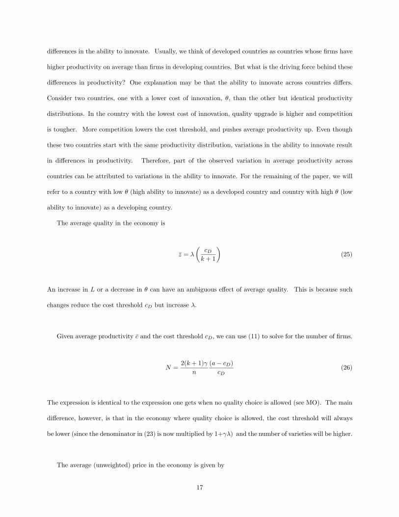
The average quality in the economy is

�z = �

�cDk + 1

�(25)

An increase in L or a decrease in � can have an ambiguous e¤ect of average quality. This is because such

changes reduce the cost threshold cD but increase �.

Given average productivity �c and the cost threshold cD, we can use (11) to solve for the number of �rms.

N =2(k + 1)

n

(a� cD)cD

(26)

The expression is identical to the expression one gets when no quality choice is allowed (see MO). The main

di¤erence, however, is that in the economy where quality choice is allowed, the cost threshold will always

be lower (since the denominator in (23) is now multiplied by 1+ �) and the number of varieties will be higher.

The average (unweighted) price in the economy is given by

17

�p = (1 + �)2k + 1

2k + 2(27)

In a world with no quality choice, average price is constant (only the second term exists). When qual-

ity choice is allowed, developing and/or large countries will have higher average price. Intuitively, for large

and/or developed countries, there are more �rms. These �rms choose high levels of quality upgrade resulting

in higher markups that push prices up. Notice that since we assumed that in this version of the model

marginal costs do not increase with quality, any increase in price comes only from increases in markups.

That does not imply however, that all prices go up. In fact, any parameter change that induces more

competition and lowers the cost threshold, causes some �rms to increase quality and markups and others to

decrease quality and markups. We discuss this in the next section.

Average markups are

�� =1

2(1 + �)

1

k + 1cD (28)

An increase in the size of the country does not necessarily imply that average markups fall. An increase

in L reduces cD, but at the same time it increases �. By substituting (23) into the expression above and

taking the derivative of �� with respect to L we can easily obtain conditions under which markups increase

or decrease in L.

Finally, average pro�ts are given by

�� = fE

�cMcD

�k(29)

18

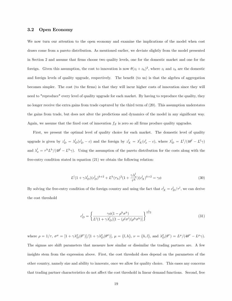
3.2 Open Economy

We now turn our attention to the open economy and examine the implications of the model when cost

draws come from a pareto distribution. As mentioned earlier, we deviate slightly from the model presented

in Section 2 and assume that �rms choose two quality levels, one for the domestic market and one for the

foreign. Given this assumption, the cost to innovation is now �(zl + zh)2, where zl and zh are the domestic

and foreign levels of quality upgrade, respectively. The bene�t (to us) is that the algebra of aggregation

becomes simpler. The cost (to the �rms) is that they will incur higher costs of innovation since they will

need to "reproduce" every level of quality upgrade for each market. By having to reproduce the quality, they

no longer receive the extra gains from trade captured by the third term of (20). This assumption understates

the gains from trade, but does not alter the predictions and dynamics of the model in any signi�cant way.

Again, we assume that the �xed cost of innovation fZ is zero so all �rms produce quality upgrades.

First, we present the optimal level of quality choice for each market. The domestic level of quality

upgrade is given by zlD = �lD(clD � c) and the foreign by zlX = �lX(c

lx � c), where �lD = Ll=(4�l � Ll )

and �lx = �hLh=(4�l � Lh ). Using the assumption of the pareto distribution for the costs along with the

free-entry condition stated in equation (21) we obtain the following relation:

Ll(1 + �lD)(clD)

k+2 + Lh(�h)2(1 +

�lx�h)(clX)

k+2 = � (30)

By solving the free-entry condition of the foreign country and using the fact that clX = clD=�

l, we can derive

the cost threshold

clD =

� �(1� �h�h)

Ll(1 + �lD)[1� (�l�l)(�h�h)]

� 1k+2

(31)

where � = 1=� , �� = [1 + ��D(��)]=[1 + ��D(�

�)], � = fl; hg, � = fh; lg, and ��D(��) = L�=(4�� � L� ).

The sigmas are shift parameters that measure how similar or dissimilar the trading partners are. A few

insights stem from the expression above. First, the cost threshold does depend on the parameters of the

other country, namely size and ability to innovate, once we allow for quality choice. This eases any concerns

that trading partner characteristics do not a¤ect the cost threshold in linear demand functions. Second, free

19

trade does not blow up the solution. Setting �h and �l to 1 causes problems only if the countries are identical

in size and/or productivity (�� = 1). Third, the degree of heterogeneity between the trading partners a¤ects

the sigmas, and therefore, a¤ects the responsiveness of the cost threshold to trade liberalization. That is,

the e¤ect that a 10% reduction in tari¤s has on cD does depend on characteristics of the trading partners,

namely how similar or dissimilar they are in size and ability to innovate. We elaborate on this later.

4 Analysis

Based on the parameterized version of the quality choice model, we proceed to show what happens to such

economies when key parameters change. First, we consider an increase in the size of the economy. Then,

we consider an increase in the ability to innovate. In both cases, we focus on the closed economy version

of the model. Looking at size and the ability to innovate helps us compare and contrast large versus small

economies, as well as developed versus developing. Next, we see what happens when an economy opens up

to trade5 .

4.1 Size and Ability to Innovate

For the sake of building intuition, suppose that at time t0 the economy is small (L) or the cost of innovation

(�) is low and at time t1 its size increases or the cost of innovation decreases. An increase in L or a decrease

in � induces more competition. This extra competition lowers the cost threshold. Some �rms now decide

to exit the market since they cannot compete. Given that the cost threshold in now lower, product variety

and average productivity increase. From the �rms that stay in the market, some are encouraged to increase

quality choice (and markups) and others to lower quality. Since the slope of the quality line is �, as L

increases or � falls, the cost threshold moves inwards and the slope increases. This is shown in Figure 2. The

black line represents quality choice at time t0 for the small or developing country. The grey line represents

5We do not analyze unilateral trade liberalizations in this version. The reason is that by assuming that export quality has

to be reproduced, we get similar results to the MO framework (although di¤erences between the trading partners will have

some impact). What makes a di¤erence is when we move to a more realistic assumption where we assume that export �rms

only have to pay the incremental cost of innovation if they choose to export goods of higher quality. In such case, unilateral

trade liberalizations do not necessarily imply less competition for the host country. This analysis is coming soon.

20

quality choice at time t1 for the large or developed country. The �rms to the right of the intersection of

the two lines represent �rms that lower their quality choice, markups and prices as a result of the extra

competition. Firms to the right are �rms that increase their quality choice and markups. Prices need not

increase for these �rms. Based on (16a), a drop in cD puts downward pressure on prices. But there is also

an upwards pressure on prices since the quality choice is now higher. Whether the total e¤ect on prices

will be positive or negative depends on Proposition 2. In contrast to MO, the extra competition does not

necessarily imply that prices and markups will fall. For some �rms this will be true, but for others it will

not be. Therefore, average prices and markups also need not fall. Notice also that the range of available

qualities is higher for rich and developed countries. This can be seen from the graph by observing that the

z-intercept is higher for the gray line than it is for the black line.

The idea that more competition encourages some �rms to upgrade quality is not new. In a series of

papers, Sutton shows that �rms in an endogenous sunk cost industry can gain market share as competition

increases. In his words (1991, p. 47): "If it is possible to enhance consumers�willingness-to-pay for a given

product to some minimal degree by way of a proportionate increase in �xed cost (with either no increase or

only a small increase in unit variable costs), then the industry will not converge to a fragmented structure,

however large the market becomes.� Sutton�s insight is re�ected in Figure 2. As the size gets bigger and

competition increases, the slope of the quality line goes up. As the slope increases, the least productive

�rms lower quality and experience a drop in their market share, but the most productive exploit the increase

in market size by adding more quality. More quality increases the consumers�willingness to pay and hence,

the �rms�market share. In the absence of quality choice however, more competition will result to market

fragmentation as �rms loose market share.

4.2 Trade

Accounting for quality choice really pays o¤ when we consider trade. As in the case of no quality choice,

opening up to trade induces more competition that raises average productivity and the number of varieties.

But now, characteristics of the trading partner, such a size and ability to innovate, matter. As we discuss

next, trading with a large country creates more competition than trading with a small country, and trading

21

with a developed country induces more quality upgrade than trading with a developing one. Adding more

structure the model enables us to consider a two-dimensional heterogeneity across countries: size and ability

to innovate.

First we discuss di¤erences between trading with a large versus a small partner. For simplicity, assume

that both trading partners have the same ability to innovate (�l�h = 1). The higher the size of the trading

partner is, the lower the production cost threshold cD and export cost threshold cX are, and the higher the

slope of the export quality choice �lX is. This is illustrated in Figure 3. The black line represents the quality

choice of domestic �rms exporting to a small country, and the grey line the quality choice of domestic �rms

exporting to a large country. Since the domestic �rms that export choose two separate levels of quality

upgrades, one for domestic sales and one for foreign, we focus and plot their choice of export quality (dashed

line). Clearly, for the large trading partner, the cost threshold is lower since competition is higher. Also, the

export threshold is lower. When the size of the export partner increases, the slope of export quality increases,

forcing the least productive export �rms to reduce export quality and encourages the most productive to

raise export quality. Although the slope of domestic quality choice does not change, the line shifts down as

a result of a drop in the cost threshold. Therefore, domestic quality upgrade choice is reduced more when

trade occurs with a large country. Notice that trade does generate the Balassa-Samuelson e¤ect. Opening

up to trade forces the least productive �rms (those that do not export) to lower price and quality due to

increase competition. It also encourages the most productive �rms (those that export) to upgrade quality,

and raise markups and prices. The larger the perceived market is with of trade (either because the partner

is a rich and/or a large country), the bigger the quality upgrade of exports will be and the bigger the drop

in price of non-exports. As a result, prices of traded to non-traded increase. This is the Balassa-Samuelson

e¤ect.

Next we discuss the impact of trade when the ability to innovate di¤ers, but size does not. Opening to

trade induces competition. The competition is higher when trade occurs with a developing country than

when it occurs with a developed country6 . Trading with a developed country creates more pro�table export

opportunities so competition is not as tough and the cost threshold does not have to fall as much. The

6This is because �l�h = 1 and and as � decreases, �h decreases and cD increases.

22

slope of both the export and domestic quality upgrade choice do not change as the � of the trading partner

varies. However, when trade occurs with a developed country, the cost threshold drops by less than if trade

occurred with a developing country, and consequently, the quality upgrade line (both domestic and foreign)

shifts up. This is the Verhoogen (2008) insight. As Mexico trades more with the US, more �rms in Mexico

have incentives to export high quality goods. Verhoogen�s insight goes through in this model, albeit in a

stronger version. Not only Mexican �rms have an incentive to increase export quality, but they also have

an incentive to increase domestic quality as well. Figure 4 illustrates the di¤erences between trading with a

developed and a developing country discussed above.

5 Conclusion:

Quality choice by �rms is important. It explains why prices increase in productivity (Baldwin and Harrigan

[2007], Johnson [2007]), why the wage gap between low and high skill labor increases in developing countries

when they trade with developed (Verhoogen [2008]), and why rich countries trade more with each other than

gravity models predict (Hummels and Klenow [2002]).

This paper presents a model of heterogeneous �rms, quality and trade. In the model, �rms not only

choose price, but they also choose the optimal level of quality they desire. To upgrade quality a �xed cost

must be paid. The level of this �xed cost is endogenous and depends on the level of quality upgrade a �rm

chooses to undertake. Markups are non-constant. A �rm can increase the consumers�willingness to pay by

adding more quality, but it has to pay a higher cost of innovation in order to obtain the extra quality. The

model is solved for both a closed and an open economy and the equilibrium is analyzed.

The model can match the insights of Verhoogen, Baldwin and Harrigan, Johnson, and Hummels and

Klenow discussed above. It also generate the Linder hypothesis. That is, there is a higher share of quality

goods produced and consumed in rich countries. The explanation comes from the supply side. It is

easier to recover the �xed cost of innovation in rich rather than poor countries. Furthermore, the model

generates the Balassa-Samuelson e¤ect. The richer the trading partners are, the higher the ratio between

the price of traded to non-traded is. Trade among rich countries encourages quality upgrade but is also

creates competition. The most productive �rms (those that export) raise quality and price, and the least

23

productive (those that do not trade) lower quality and price. The model is also consistent with the Sutton

(89, 91) insight that in endogenous sunk costs industries, competition does not necessarily imply market

fragmentation. When �rms are allowed to upgrade quality, we observe that productive �rms can respond to

the pressure of competition by paying a higher �xed cost of innovation, di¤erentiating their products more,

and increasing the consumers willingness to pay and their market share. Finally, when the quality choice

of �rms is taken into account, we see that trading partner�s characteristics a¤ect the level of competition in

the home country, as well as the cost threshold between the �rms that produce and the ones that do not.

And since the cost threshold changes, all other parameters in the economy such as product variety, average

productivity, price and markups change. This would not be true if quality choice is not accounted for (Melitz

and Ottaviano [2007]) or if quality is accounted for but markups are kept constant (Johnson [2007]).

24

References

[1] Baldwin, R. and J. Harrigan, 2007. "Zeros, Quality and Space: Trade Theory and Trade Evidence,"

NBER Working Papers 13214

[2] Bernard. A. B, S. J. Redding, and P. K. Schoot (2006) "Multi-Product Firms and Product

Switching" NBER Working Paper 9789

[3] Bilbiie, F., M. Melitz, and F. Ghironi (2007) "Endogenous Entry, Product Variety, and Business

Cycles" Working Paper

[4] Choi. Y. C., D. Hummels, and C. Xiang (2006) "Explaining Import Variety and Quality: The Role

of the Income Distribution" Working Paper

[5] Hallak, J. C (2006) A Product-Quality View of the Linder Hypothesis" Working Paper

[6] Hummels, D. and P. J. Klenow, 2002. "The Variety and Quality of a Nation�s Trade," NBER

Working Papers 8712

[7] Johnson, Robert. 2007 "�Endogenous Non-Tradability and International Prices: An Empirical Ex-

ploration of the Melitz Model" Working Paper

[8] Khandelwal, A. (2008) "The Lond and Short (of) Quality Ladders," mimeo, Columbia University

[9] Melitz. M. J. (2003) "The Impact of Trade on Intra-Industry Reallocations and Aggregate Industry

Productivity�, Econometrica, vol. 71, November 2003, pp. 1695-1725

[10] Melitz, M. and G. Ottaviano (2007) �Market Size, Trade, and Productivity�, Review of Economic

Studies, vol. 75, no. 1, pp 295-316

[11] Murphy, K. and A. Schleifer (1997) "Quality and Trade" Journal of Development Economics, June,

1997

[12] Schott, P. (2004) "Across-Product Versus Within-Product Specialization in International Trade",

Quarterly Journal of Economics, vol 119, pp 647-678

25

[13] Sutton, J. (1989) "Endogenous Sunk Costs and the Structure of Advertising Intensive Industries",

European Economic Review, vol 33, no 2, pp. 335-344

[14] � � � � , (1991) "Sunk Costs and Market Structure," Cambridge, MA, MIT Press

[15] Verhoogen, E. (2008) "Trade, Quality Upgrading and Wage Inequality in the Mexican Manufacturing

Sector.�Quarterly Journal of Economics, vol. 123, no. 2, May 2008.

26

Figure 1: Graphical Representation of Quality Choice for a Given Cost Level

Quality Upgrade, z

cZ cD

z

0

Marginal Cost, c

Produce Output No Quality Upgrade

Exit Produce Output and Quality Upgrade

Figure 2: Quality Choices in a Closed Economy as L Increases or θ Falls.

Cost, ccD c'

D

Small/ Developing

Large/ Developed

slope =λ

Quality Choice (z)

Figure 3: Quality Choice as the Size of the Trading Partner Increases

Cost, ccD c'D

Small

Large

cx c'X

Quality Choice (z)

Figure 4: Quality Choice as the Ability to Innovate of the Trading Partner Increases

Cost, ccD c'D

Developing Developed

cx c'X

Quality Choice (z)