Competition in Banking:

Exogenous or Endogenous Sunk Costs?

Astrid A. Dick∗

This version: July 2004

Abstract

Testing the theory of Sutton (1991), this paper presents empirical evidence consis-

tent with the predictions of the endogenous sunk cost model of competition, with an

application to banks. In particular, banking markets remain concentrated regardless of

market size. Given an asymmetric oligopoly where dominant and fringe firms coexist,

the number of dominant banks remains unchanged with market size, with only the

number of fringe banks increasing with market size. Such structure is sustained by

competitive investments in advertising and quality, with the level of these increasing

with market size and dominant banks providing a higher level than fringe banks. Our

findings indicate that the expansion of sunk investments in advertising and quality,

and not exogenous scale economies or horizontal differentiation, explain the persis-

tent concentration observed in the banking industry. The analysis has implications for

antitrust policy.

∗Division of Research and Statistics, Federal Reserve Board, Washington, D.C., astrid.dick@frb.gov.This paper is based on earlier work titled “Market Structure and Quality: An Application to the BankingIndustry,” from the author’s PhD dissertation. The author is grateful to Susan Athey, Evren Örs and NancyRose for their insightful comments. She would also like to thank Allen Berger, Steve Berry, Paul Ellickson,Timothy Hannan, Michael Salinger, as well as participants at the International Industrial OrganizationConference, Federal Reserve Bank of Chicago Bank Competition and Structure Conference, and FederalReserve Bank of New York for their suggestions. The views herein, as well as any errors, are the author’s.

1 Introduction

The work of Sutton (1991) provides a theoretical framework to explain why some markets

remain concentrated as they grow in size, while others fragment. The theory discriminates

among industries by analyzing the interplay of exogenous and endogenous elements of sunk

costs. When the latter, such as advertising or quality investments that are fixed with respect

to output, are significant relative to the setup costs of the firm, the theory predicts that mar-

ket concentration will not fragment but rather converge to a strictly positive value as market

size grows, with quality investments per firm increasing with market size. By categorizing

industries into either exogenous or endogenous sunk cost competition based solely on a few

observables, the theory provides insight into the process behind a given market structure as

well as the nature of competition among firms.

While Sutton’s work makes robust predictions across a broad class of competition models

about the relationship between market concentration and market size, empirical research

testing these predictions has nevertheless been scant. Sutton (1991) provides a cross-country

analysis of various industries in trying to find empirical counterparts to the theory, thus

confronting many of the measurement problems typical of such cross sections. Ellickson

(2001) applies the Sutton framework to the empirical study of U.S. supermarkets. His work

is the first to test the theory’s predictions on a large data set of markets within a single

industry. Recently, Berry and Waldfogel (2003) examine the relationships between market

size and product quality in the newspaper and restaurant industries, where the quality

production processes are believed to differ.

This paper uses Sutton’s framework to build on the empirical work in the literature, with

an application to the banking industry,1 taking a cross-section of U.S. metropolitan markets.

The theory, providing clear and concise predictions, allows for a formal test of the nature of

competition characterizing banking markets. The banking industry is a good application

because of the large number of geographically distinct markets of varying sizes, and the

available bank level data. Moreover, it is an industry where we expect both exogenous

and endogenous sunk costs to be relevant, with both horizontal and vertical differentiation

1On a different vein, Gual (1999) tests a model related to Sutton to analyze the impact of deregulationin European banking markets.

1

potentially affecting the observed market structure.

The results suggest that the industrial structure of banking markets can be explained by

the endogenous sunk cost model. In particular, there exists a lower bound to concentration

which converges asymptotically to a positive value, with banking markets exhibiting similar

concentration levels across all market sizes. This market structure appears to be sustained

by competitive investments in advertising and quality, including employee compensation,

branch networks, branch staffing and geographic diversification, with the level invested per

firm increasing with market size. Moreover, there is an asymmetric, dual structure in the

market characterized by the coexistence of a few and regional dominant banks — defined

as those banks with the largest shares who jointly control over half of the deposits in a

given metropolitan market — with a number of small and local banks which constitute a

fringe. Given this concentrated structure of asymmetric oligopoly, the equilibrium number

of dominant banks remains unchanged with market size, with only the number of fringe

banks varying across markets. Dominant banks are also found to advertise more intensively

and provide a higher level of quality than fringe banks. Furthermore, banks do not appear

to carve out areas within the relevant geographic banking market, but rather compete with

each other closely. In terms of the product market, however, dominant and fringe banks

appear to focus on a few different sectors.

The analysis has some direct implications for antitrust policy. The introduction of quality

investment in the study of competition alters the interpretation of certain empirical corre-

lations between the number of firms, market concentration and conduct used in antitrust

policy. For instance, the finding that markets with fewer firms tend to have lower deposit

rates and higher loan rates has been historically taken to imply a less competitive conduct

by banks and therefore a bad thing for consumers. However, once quality is controlled for,

there is no unambiguous implication one can make about consumer welfare from the empiri-

cal correlation between prices and the number of banks in a market. In fact, one could easily

envision banks charging higher prices for a higher quality service that consumers are happier

with. Moreover, antitrust authorities focus on market concentration to determine whether

a contemplated merger might cause antitrust concerns. In the context of the present paper,

a relevant question might be whether the new bank would provide a higher level of quality,

2

and whether it would become a dominant firm or join the fringe. For example, will the

merger increase the ATM network available to consumers and the levels of advertising that

consumers might enjoy? Will the formation of the new firm imply the reduction of the

number of dominant firms to one? If the post-merger firm becomes dominant, will it have

competition from other dominant firms?

This paper also sheds light on the empirical finding that larger banks charge significantly

higher fees than smaller banks [such as Hannan 2001, 2002]. The reasons usually speculated

for this occurrence include locational differences between larger and smaller banks, the better

service quality of bigger banks, and the fact that larger organizations tend to depend less on

retail customers for funds. The findings here indicate that dominant firms, which tend to

be large banks, do charge higher fees yet advertise heavily and invest more in quality.

The rest of the paper is organized as follows. Section 2 outlines the theoretical framework.

Section 3 describes the data and provides a discussion of sunk costs in banking. Section 4

takes the predictions of the Sutton theory to the banking data, providing a robustness

analysis as well as exploring alternative explanations to the findings. Section 5 provides an

analysis of competition inside banking markets, while 6 analyzes some of the implications

for antitrust policy. Finally, section 7 concludes.

2 Theory of market structure and quality

The work of Sutton (1991)2 provides a robust framework that allows us to categorize the

type of competition in an industry based on the observed relationship between market con-

centration and market size. This theory guides the empirical analysis in this paper. Central

to it is the notion that some sunk costs are incurred with a view to enhancing consumers’

willingness-to-pay for the firm’s products, and as a result represent a firm’s choice variable

and are “endogenous.” The key to the theory is that while exogenous sunk costs have a

fixed magnitude irrespective of market size, endogenous sunk costs do vary with market

size —though both are fixed with respect to output. Drawing a distinction between these

sunk costs, the model makes predictions, across a broad class of competition models, about

2Sutton (1991) builds especially on two earlier papers by Shaked and Sutton (1983, 1987).

3

the relationship between market concentration and market size, as well as the equilibrium

investment in endogenous sunk costs.

Exogenous sunk costs, on the one hand, are defined as those setup costs or fixed outlays

associated with acquiring a single plant of minimum efficient scale, which do not vary with

market size. Endogenous sunk costs, or quality investments whose magnitude is chosen by

the firm, on the other hand, are defined as costs that can change a firm’s demand and require

a fixed cost but no or little increase in unit variable costs. Examples of endogenous sunk

costs are advertising, R & D, and any product feature that increases the amount consumers

are willing to pay for the firm’s product relative to rivals’ products. The central focus of the

theory then lies in unraveling the way in which these two elements of sunk costs, exogenous

and endogenous, interact with one another to determine the equilibrium market structure in

an industry.

For the case of exogenous sunk costs, the central prediction of the theory is that an

increase in market size relative to setup costs may lead to indefinitely low levels of market

concentration.3 In the case of endogenous sunk costs, however, this property breaks down.

Here the model predicts that markets remain concentrated regardless of market size, as com-

petition among firms leads to escalating investment in quality. In particular, the conclusions

of the model are:

(1) Market structure does not fragment as market size increases, and therefore there exists

a lower bound to the equilibrium level of concentration in the industry, no matter how large

the market becomes;

(2) firms engage in a competitive escalation of investment in quality as market size increases;

(3) the equilibrium number of firms in the market remains approximately the same regardless

of market size.

Model

While Sutton considers the case of industries with solely exogenous sunk costs, in reality,

endogenous sunk costs are a business decision variable in all industries. One way to capture3In an industry where there are only fixed setup costs and the product is homogeneous, the equilibrium

number of firms should increase with market size, while market concentration should asymptote to zero. Ina horizontally differentiated product setting, however, the existence of only exogenous components to sunkcosts leads to multiple equilibria, ranging from concentrated to fragmented market structures.

4

this is by measuring the significance of endogenous costs relative to the setup costs of the

firm. The model of Schmalensee (1992), which is used here to illustrate Sutton’s theory,

allows for this kind of analysis. The degree of importance of sunk costs is a parameter of

the model, such that competition is determined by the competitive escalation of endogenous

sunk costs as long as market share is sufficiently sensitive to variations in these fixed costs

(so that firms compete mostly on fixed outlays as opposed to per-unit price-cost margins).

This framework is particularly useful here as it embodies the two kinds of industries Sutton

studies but does so in a single model, providing specific predictions for both cases that we

can then take to the data.

Following Schmalensee (1992), assume an industry with free entry andN ex ante identical

firms. Firm i’s profits are given by:

πi ≡ (P − c) ∗ qi(Ei)−Ei − σ

where price, P, is assumed exogenous4 (set in earlier stage)5, c is a constant per unit cost, σ

is a fixed setup cost, and Ei represents the endogenous sunk cost investment which shifts de-

mand, such as advertising. The firm’s unit sales, qi, which are a function of this endogenous

sunk cost investment, are given by:

qi(Ei) = S

"Eτi /

NXj=1

Eτj

#

where S is the size of the market and the firm’s market share is in brackets (which may be

thought of as arising from a random utility model) and depends on Ei. The parameter τ ,

where τ > 0, represents the toughness of endogenous sunk cost competition, and captures

how sensitive market share is to demand shifting expenditures.

4As Schmalensee points out, note that the results are robust to alternative models of price competition,such as assuming that (P − c) is some decreasing function of N (an increasing number of firms puts extrapressure on margins, and therefore N grows more slowly with market size), a reasonable assumption.

5This dynamic structure is chosen by Schmalensee (1992) as he argues that a more short-lived advertisingchoice is reasonable based on advertising budgets usually responding periodically to market conditions, whileprices exhibit some rigidity. The latter appears to be a good assumption for the banking industry, whereprices, especially on the deposit side, tend to exhibit some rigidity, especially downwards [Hannan and Berger(1991); Neumark and Sharp (1992)]. Schmalensee also cites empirical evidence for the fact that the effectsof advertising are not very long-lived.

5

There are well-behaved symmetric Nash equilibria in the Ei with π ≥ 0 for 0 ≤ τ ≤ 2.Setting E∗i = E∗ = (P−c)Sτ

N

£1− 1

N

¤, from the zero profit condition we have:

(1/N∗)(1− τ) + (1/N∗)2τ − (σ/S)(1/(P − c)) = 0.

For the range τ ≤ 1, the predominant form of competition is in exogenous sunk costs:

N∗ →∞ as S →∞, so that market concentration converges asymptotically to zero, and, asmarket share is not very sensitive to E, the ratio of endogenous sunk cost expenditure with

respect to output is low.6

For 1 < τ ≤ 2, the predominant form of competition is in endogenous sunk costs:

N∗ → τ/τ − 1 as S → ∞, so that market concentration is bounded away from zero,

converging to a strictly positive value. Moreover, investments in endogenous sunk costs

are high and grow with S. The idea is that the larger is τ , all else equal, the higher are the

endogenous sunk expenses per firm and the lower the profits, so that in equilibrium there is

a lower number of firms.

More generally, the testable implications from the model for banking markets are as

follows. If competition is predominantly through exogenous sunk costs, then we should

observe lower levels of concentration in larger cities. If competition is mainly through

endogenous sunk costs, in the sense that demand is responsive to a firm’s investment in

advertising or some other quality enhancing expenditure, then we should observe high levels

of concentration even in larger cities as well as a higher level of advertising and quality. In

the following sections, these empirical implications are taken directly to the banking data.

3 The banking industry: data and background6Note that when τ = 1, as S → ∞, N also grows but at a slower rate, since N∗ =

p(p− c)S/σ, such

that E∗grows but not as fast.

6

3.1 Data sources

The data are based on a cross-section for 19997 and are taken from several sources. The

variables used here to analyze market structure include: 1) bank characteristics, derived

from balance sheet and income statement information from the Report of Condition and

Income (Call Reports) from the Federal Reserve Board; 2) branch deposits, taken from the

Federal Deposit Insurance Corporation (FDIC) Summary of Deposits; and 3) demographic

variables, taken from the U.S. Census, the Bureau of Economic Analysis and the Office of

Federal Housing Enterprise Oversight. The sample includes all metropolitan markets and

all FDIC insured-commercial banks in the U.S. The Appendix shows summary statistics for

the variables used in the analysis, as well as a description of the variables.

Given the format of the data, there are several possible levels of aggregation that could

be used as the unit of analysis. My approach is to define the relevant geographic banking

market at the level of the metropolitan statistical area (MSA), a geographic unit defined by

the U.S. Census Bureau that consists of a large population nucleus, together with adjacent

communities, that comprise one or more counties. This market definition is supported by

surveys of consumers and businesses as well as the bulk of the empirical banking literature.8

3.2 Basic characteristics of banking markets

In the U.S. there are about 330 MSA banking markets, which represent 83 percent of total

U.S. dollar deposits. These markets are geographically distinct and largely independent.

While some banks in the U.S. operate in various markets, the bulk of banks have presence in

only one or two markets.9 Even for those banks that operate in more than one market, usu-

ally demand conditions, and to some extent cost factors, are independent across markets.10

The average number of banks in an MSA is 20, with as few as two banks in Lewiston-Auburn,

7The data are for the second quarter, which is chosen here because some the variables of interest arereported only then.

8For a detailed discussion on relevant geographic market definition, see Dick (2002) and the referencestherein.

9Close to 65 percent of banks operate in a single MSA market.10While the evidence suggests that multimarket banks do tend to set uniform prices across large geographic

areas [Radecki (1998), Heitfield (1999), Biehl (2000)], they are assumed to do so by responding to local marketconditions across all markets served, such that the uniform price is a weighted average of these.

7

ME, and with as many as 255 in Chicago, IL. Table 1 shows the distribution of MSA mar-

kets in terms of the number of banks in the market. On average, an MSA has a total of

140 branches. Adjusting by population, there is an average of 28,000 persons per bank in a

given MSA, and 4,600 per branch. As measured by population, the bulk of markets has a

size between 100,000 and 500,000 people.11 Table 2 shows a tabulation of MSAs by various

population size categories.

The average Herfindahl-Hirschman index (HHI)12 across MSA markets is around 1900,

with market concentration going from as low as 584 in Chicago, IL, which has 255 banks, to

almost 7800 in Pittsfield, MA with only three banks.13 The largest deposit share in a given

market (C1) is an average of 0.31 or 31 percent. The last two columns of Table 2 shows the

average HHI and C1 for each market category by population, while Table 3 depicts some

percentiles for the distribution of the HHI (st. dev. of 800) and C1 (st. dev. of 0.1) across

MSA markets.

Definitions: dominant and fringe firms

Banking markets usually hold dozens of firms, with great variation in their market shares,

and with many firms holding only a very small portion of the market. This is likely to give

rise to an asymmetric oligopoly structure, which will be explored later in the paper. For

this purpose, I define two types of banking firms that will be used in the analysis: dominant

and fringe. Dominant firms are the set of leading banks with the largest market shares

which jointly hold over half of the market’s deposits. All other firms are fringe firms. For

robustness purposes, some other definitions of dominant firms will be used as well later in

the analysis.14

11The average MSA size is about 1940 square miles.12The Herfindahl-Hirschman index is a concentration measure constructed as the sum of the squares of

the market share of deposits at the local market level. Here, following the practice of the Antitrust Division,I multiply it by a factor of 10,000.13The Antitrust Division defines the threshold of a highly concentrated market at 1800.14In particular, two other definitions of dominant firm will be utilized to test whether the results here are

sensitive to the definition of dominant firm given in the text: (i) following the Department of Justice and theFederal Reserve Board’s definition, a dominant bank is that whose market share is at least twice as large asthe share of the second-largest competitor in the market (from the “Casework Manual” for merger proposalsof the Federal Reserve Board); and (ii) a dominant firm is that with the largest market share in a market(or alternatively, those with the largest two/three market shares).

8

Market equilibrium

Sutton’s theory of market structure applies to markets in equilibrium. In the case of

the banking application here, the underlying assumption is that the industry reached an

equilibrium in 1999, the year of the analysis. While changes in the industry continued

to occur after 1999, the assumption seems reasonable given the tremendous shake-out the

sector experienced throughout the last three decades, and in particular in the last ten years,

with the introduction of nationwide branching throughout 1994-1997.15 Figure 1 shows the

number of bank mergers per year since 1993.16 There is an average of 360 mergers per

annum, and the number of mergers per year decreases steadily since 1994. Moreover, in

1999, there is a decrease of over 60 percent in the number of mergers from the previous year,

and of 70 percent since 1993.

There are a few caveats to note about this assumption. First, mergers take a while to

settle, and mergers do occur in 1999. Second, 1999 is a boom year in the business cycle.

However, the market structure in 1993 (in terms of a dominant firm vs. fringe framework)

is found to be similar to that of 1999, even though 1993 is not a boom year.

In addition, I find that the firms that have negative (accounting) profits in 1999 and that

would likely exit the market, are part of the fringe. As a result, the basic market structure

between dominant and fringe firms, documented later in this paper, should not be affected

by these developments in the industry in any significant manner.

3.3 Exogenous and endogenous sunk costs in banking

The setup costs involved in opening a bank in the US are small relative to other industries.

While there appears to be no legal minimum and there is great variation across states and

local areas, the amount of capital needed to start a bank averages around 7 million dollars,

15Regulatory restrictions affecting the ability of banks to diversify geographically have decreased dramat-ically. Deregulation of unit banking and limited branch banking occurred gradually throughout 1970-1994in most states. Intrastate branching deregulation began in some states even before the 1970’s, while inter-state banking started as early as 1978. The process of deregulation of geographic expansion culminated in1994 with the passage of the Riegle-Neal Interstate Banking and Branching Efficiency Act, which permittednationwide branching as of June 1997.16The information on the figure is based on the author’s calculation using Banking Holding Company data

from the Federal Reserve Board.

9

a small portion of which are actually sunk costs such as filing fees, branch construction

costs, and legal fees.17 The process takes at least 7 months, and it includes: (i) forming the

organizing group (usually with a minimum of 5 individuals) that are capable of jointly holding

at least a quarter of the bank’s capital; (ii) submitting an application to the corresponding

regulatory authority (based on the type of charter chosen) with a filing fee of around $15,000;

(iii) regulatory review; (iv) raising capital; and (v) regulatory approval.

In terms of endogenous sunk costs, a cost incurred by a bank to enhance its service

qualifies as endogenous if it mostly involves an increase in fixed outlays, possibly accompanied

by a limited increase in unit variable costs. Advertising and branding expenditures are a

good example in the industry, but also the branch and ATM network, among others. The

latter can be interpreted as endogenous sunk costs as long as banks open branches mostly

in response to their own quality and market targets, as opposed to their existing customers’

needs, with branches usually operating below capacity. The anecdotal evidence appears to

support this assumption.

Banks differ greatly in terms of the advertising and the service quality they provide to

their customers. Within a given market, a set of very diverse banks tend to coexist, with

some being small, local banks with a few branches, and others big brand names covering

large geographic areas with extensive ATM and branch networks. Banks also differ in terms

of the expertise and customer care offered at the branch, the size of branch personnel (which

is related to the availability of human interaction and waiting times), financial advise and

overall service quality.

Advertising and Branding

Advertising and developing a brand name is likely to be an important component of a

bank’s endogenous sunk costs. Though one feature that stands out is the degree of hetero-

geneity across banks in terms of their investment in advertising. According to surveys carried

out by the American Bankers Association, roughly one percent of bank operating costs, on

average, was devoted to advertising in 1996, while total bank marketing expenditures were

17Based on anecdotal evidence from Richardson, C. (2003), “5 Phases of De Novo Formation,” Bankmarkand Startabank.com (www.nubank.com). The amount of capital also depends on the type of charter andfinancial institution chosen, as well as the types of services the bank wants to provide.

10

close to 4 billion dollars in 2001. Anecdotal evidence suggests that in the nineties “[bank]

marketing has moved from a back room operation ... to a front line strategic function.”18

For instance, according to National Leading Advertising, BankAmerica Corp. was the 125th

leading U.S. advertiser in 1996, with total expenditures of $145 million. Further evidence

suggests that banks invest a growing fraction of their advertising resources by engaging in

branding campaigns and brand building, as well as the development of in-house brand mar-

keting departments and branding strategies.19 The importance of branding in banking is

further signified in the way banks that merge choose their new brand name, where they keep

the name that customers are more familiar with and/or is the strongest brand, according to

bank periodicals.20

Given the scarcity of advertising data, there is no academic work in the area, with the

exception of Örs (2003), who analyzes the role of advertising in commercial banking using

new data on bank advertising for the period 2001-2002. Örs finds that advertising increases

bank profitability, thus concluding that nonprice competition through advertising plays an

important role in the industry.

Moreover, advertising outlays are likely to be correlated with the number of bank branches,

based on the anecdotal evidence on the greater role of the branch in the bank’s advertising

decisions.21 As described by Radecki et al. (1996), a typical branch has expenses of around

$700,000 per year, and while the largest component of this cost is staff compensation, ad-

vertising is usually part of it. Indeed, branches are to banks a form of advertising itself.

There is plenty of anecdotal evidence about how banks hope to woo customers using their

branches, usually with stylish merchandising and customer service.22 Banks become more

18“The Banks, They Are A’ Changin’,” D. Asher, Newspaper Association of America, 2003.19For example, a search on bank branding on the American Banker magazine database throws out thou-

sands of related articles for recent times, suggesting the prevalence of branding as a part of bank business.20A good example is that of the large NationsBank and BankAmerica merger in 1998: they chose the

BankAmerica name because of “its longer history” and “its patriotic feel which has more intrinsic appealthan the NationsBank name” [“Brand Name to Be Unveiled in Ads Tonight,” C. Guillam, American Banker,Sept. 30, 1998].21“With micromarketing, the promotional decisions are shifted from the corporate staff to the individual

branches, where more is known about customers and prospects, such as where they live and what they buy...There are less [sic] expensive television commercials and highly effective outdoor displays” (from “It Pays toThink Small in Marketing,” K. Pelz, American Banker, March 4, 2002).22For example, “... a handful of large institutions are planning aggresive campaigns to build market share”

(“Some Giants Planning Ad Assaults; They Hope to Gain Market Share as Others Retrench,” E. Braitman,American Banker, November 15, 1990). As part of this strategy, many banks have even tried installing

11

visible to consumers through their branches, and in fact, many banks put clocks outside

their branches for this reason.

Branch and ATM network

At least some of the branch and ATM installation costs, which affect the bank’s demand

by attracting new customers, are clearly sunk (net of any resale value23). Once built, it

is hard to recoup the incurred costs. As Radecki et al. (1996) point out, the typical

bank branch costs roughly $1 million to build. While a portion of this expense is for

equipment, which may be removed and installed elsewhere, most of it covers construction

costs. There is also plenty of anecdotal evidence suggesting that branches represent sunk

costs. For instance, it represented one of the main arguments for internet banking (The

European Internet Report, Morgan Stanley Dean Witter, June 1999).24

While the cost of opening a single branch might not be exactly fixed with respect to

output, a bank’s overall branch density cost is likely to be largely independent of output

levels. In other words, branch networks are at least somewhat independent of the number of

customers using them in the sense that while a consumer might do most of her banking with

a single bank branch, she should still value the convenience of her bank’s branch density in

the area as well as its ATM network. Moreover, while in theory there exists a maximum

number of customers that a single branch can service (or, for that matter, that a given

employee or computer system memory can serve), it is unlikely to be binding in practice.

This is suggested by the popularity in recent years of the in-store or supermarket branch —a

full service branch located within a large retail outlet— as a way to expand customer bases

relative to a conventional bank branch [Radecki et al., 1996]. Banks find them attractive

not only for cost reduction purposes, but also because they provide access to large flows

of potential and existing customers (even though they have smaller staffs than branches):

the typical supermarket averages 20,000 to 30,000 customers a week, while the typical bank

branch averages just 2,000 to 4,000 weekly customers [Williams, 1997].

coffee shops and “investment bars” within their branches (“Bank branches take a page from retail’s book,”San Francisco Business Times, Sept. 2001).23Some of the cost of branches could later be recouped if the bank is able to sell them in a merger or

acquisition.24See also Sullivan (2001), based on a survey of banks and their web site services.

12

Data

The data available do not allow for a complete and direct measure of endogenous sunk

costs, but some observable bank characteristics provide an approximation. While some of

the measures are far from perfect, many types of investments, other than advertising, are

explored here.

Advertising expenditures data are available starting in 2001 for some banks. In particular,

banks with advertising expenditures-to-operating income over 1% are required to report their

advertising expenditures to the supervisory authorities starting December 2001. While these

data are available for a subset of banks, the correlation between other noninterest expenses

— which includes advertising and is reported by all banks in our sample— and advertising is

close to 1. This can be appreciated in Table 4, where the correlation between advertising

expenditures and other noninterest expenses is provided for the years 2001 and 2002, based

on the sample of all reporting banks.25 Many of the reporting banks — over 35%— report

even though they are not required to.26 As a result, other noninterest expenses is used here

as a proxy for advertising expenditures, and divided by the bank’s deposits to get a proxy

of advertising intensity, the variable used in the regression analysis below. Advertising is

likely our cleanest measure of quality, given that it is unrelated to the number of customers

of a bank: an ad has a given price regardless of how many people it reaches or how many

get to see it.

Moreover, I use several bank attributes as quality correlates, including: (i) a bank’s

branch density in the MSA market, defined as the number of branches per square mile in the

MSA; (ii) the number of employees per branch; (iii) the geographic diversification, measured

as the number of states in which the bank operates; and (iv) salary per employee. The first

four of these quality measures have been used and found to significantly affect the consumer’s

choice of depository institution in Dick (2002), who uses a structural product differentiated

demand model.

From the consumer’s perspective, more of each one of these attributes is likely to be a

25Advertising data are reported by about half of all commercial banks in each year.26Advertising represents, on average, 5% of other noninterest expenses. Other items included in “other

noninterest expenses” are: data processing fees (13 percent); directors’ fees (4 percent); printing, stationaryand supplies (5 percent); postage (3 percent); legal fees and expenses (3 percent); FDIC deposit insuranceassessments (1 percent).

13

good thing. Branch density and geographic diversification embody the size of the overall

bank network, and therefore the convenience to the consumer. The number of employees per

branch captures some of the quality provided at the branch, since the larger the branch staff,

the lower waiting times are and the greater the availability of valued human interaction.

Salary per employee is used here as an alternative measure of quality unrelated to bank

size. In particular, salary paid to the bank’s employees should be correlated to quality, as

more highly qualified employees, who can provide better service and expertise, are more

expensive. This could also be correlated with the degree of sophistication of the products

offered by the bank. Since one would expect larger cities to have higher wages, salary per

employee is also adjusted for local costs, using housing prices.

4 Empirical results: market structure, quality andmar-

ket size

4.1 Market structure across market sizes

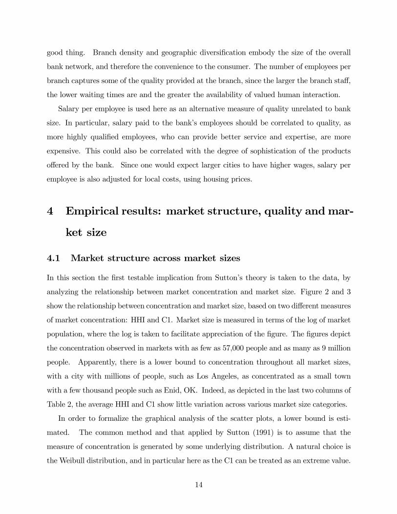
In this section the first testable implication from Sutton’s theory is taken to the data, by

analyzing the relationship between market concentration and market size. Figure 2 and 3

show the relationship between concentration and market size, based on two different measures

of market concentration: HHI and C1. Market size is measured in terms of the log of market

population, where the log is taken to facilitate appreciation of the figure. The figures depict

the concentration observed in markets with as few as 57,000 people and as many as 9 million

people. Apparently, there is a lower bound to concentration throughout all market sizes,

with a city with millions of people, such as Los Angeles, as concentrated as a small town

with a few thousand people such as Enid, OK. Indeed, as depicted in the last two columns of

Table 2, the average HHI and C1 show little variation across various market size categories.

In order to formalize the graphical analysis of the scatter plots, a lower bound is esti-

mated. The common method and that applied by Sutton (1991) is to assume that the

measure of concentration is generated by some underlying distribution. A natural choice is

the Weibull distribution, and in particular here as the C1 can be treated as an extreme value.

14

Based on the study of limiting distributions, the distribution of extreme values converges

asymptotically to a Weibull. As maximum likelihood estimation does not work for some

ranges of the parameters of the Weibull (no local maximum), I use a method developed by

Smith (1985, 1990).27

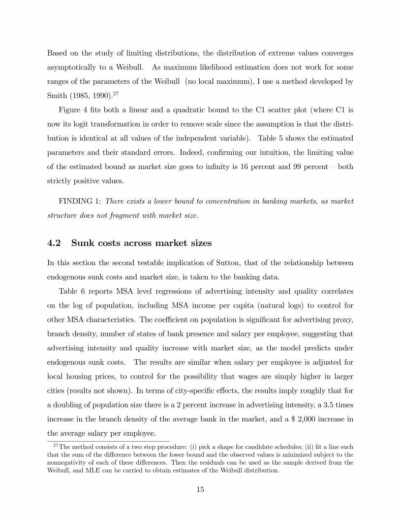
Figure 4 fits both a linear and a quadratic bound to the C1 scatter plot (where C1 is

now its logit transformation in order to remove scale since the assumption is that the distri-

bution is identical at all values of the independent variable). Table 5 shows the estimated

parameters and their standard errors. Indeed, confirming our intuition, the limiting value

of the estimated bound as market size goes to infinity is 16 percent and 99 percent — both

strictly positive values.

FINDING 1: There exists a lower bound to concentration in banking markets, as market

structure does not fragment with market size.

4.2 Sunk costs across market sizes

In this section the second testable implication of Sutton, that of the relationship between

endogenous sunk costs and market size, is taken to the banking data.

Table 6 reports MSA level regressions of advertising intensity and quality correlates

on the log of population, including MSA income per capita (natural logs) to control for

other MSA characteristics. The coefficient on population is significant for advertising proxy,

branch density, number of states of bank presence and salary per employee, suggesting that

advertising intensity and quality increase with market size, as the model predicts under

endogenous sunk costs. The results are similar when salary per employee is adjusted for

local housing prices, to control for the possibility that wages are simply higher in larger

cities (results not shown). In terms of city-specific effects, the results imply roughly that for

a doubling of population size there is a 2 percent increase in advertising intensity, a 3.5 times

increase in the branch density of the average bank in the market, and a $ 2,000 increase in

the average salary per employee.27The method consists of a two step procedure: (i) pick a shape for candidate schedules; (ii) fit a line such

that the sum of the difference between the lower bound and the observed values is minimized subject to thenonnegativity of each of these differences. Then the residuals can be used as the sample derived from theWeibull, and MLE can be carried to obtain estimates of the Weibull distribution.

15

These results suggest that there is a pivotal role for endogenous sunk cost competition

in banking, driven by a high sensitivity of demand to advertising and quality. While there

is a dearth of empirical evidence on the effects of bank advertising, the results are consistent

with the evidence in Örs (2003), where advertising expenditures are found to be related to

bank profitability. In addition, they are consistent with the evidence in Hannan and Prager

(2004) of higher prices (lower deposit rates) in larger markets, since higher advertising outlays

demand higher prices. Moreover, it is coherent with a nonmonotonic concentration schedule

as market size grows: the fact that the lower bound to concentration was found earlier to be

upward sloping can be explained by a large sensitivity of demand to fixed costs outlays like

advertising — or, alternatively, to a diminishing returns to advertising that are low.

FINDING 2: The level of bank investment in endogenous sunk costs increases with market

size.

4.3 Asymmetry and number of firms across market sizes

In this section I explore further the industrial structure of banking markets by analyzing

asymmetry among firms.

Table 7 presents a tabulation of markets according to population and number of dominant

firms.28 This table provides evidence of a striking fact: regardless of market size, the bulk

of markets (87 percent of the MSAs) have either two or three dominant firms.29 Moreover,

the correlation between the population and the number of dominant firms in a market is

almost zero. This is particularly interesting when contrasted with a model without quality

competition but just exogenous fixed costs, where the number of firms should grow with

market size given that the number of consumers served per firm should be the same for all

markets.28Ellickson (2001) finds a similar structure for supermarkets.29The results of this section hold using a few other definitions of dominant firm. In particular, following

the Department of Justice and the Federal Reserve Board’s definition, a dominant bank is defined as thatwhose market share is at least twice as large as the share of the second-largest competitor in the market(only 57 banks fall into this category, however), and as alternative definitions, a dominant firm is definedas that with the largest market share in a market (or alternatively, those with the largest two/three marketshares).

16

Deposit Lorenz curves30 provide another way to appreciate the fact that few firms control

most of the market, regardless of the number of firms serving it. Figure 5 shows a Lorenz

curve for deposits, where firms are ranked on the x-axis according to their share of market

U.S. dollar deposits, while the y-axis shows the cumulative share of deposits. Given the

large number of MSA markets, for ease of analysis the figure depicts only six markets, one

for each market size category31 (as defined in Table 2). The only apparent difference among

the markets is in the length of the tail of the curve, which grows in the number of firms

serving the market. Below the 50 percent cumulative share line, markets differ little.

The above description indicates that as markets grow, the number of dominant banks

remains virtually unchanged. Naturally, as markets grow in population size, they also tend

to expand in the number of banks, yet this growth is only reflected in the length of the

tail of the fringe, and does not affect the dominant-firm fringe structure observed in smaller

markets. Indeed, the number of firms in a market is highly correlated with population size

(0.77), yet the number of dominant firms is almost independent of population and the total

number of firms in the market.

Table 8 shows means for the various components of the measure of quality, for both

dominant and fringe firms. Dominant banks appear to advertise more intensively, as well as

provide more branches, that are also more highly staffed, be more geographically diversified,

and pay higher salaries to their employees.32 To test for the significance of these attribute

differences, Table 9 shows the results from estimating quality correlates of bank j in marketm

as a function of an indicator variable for whether the bank is a dominant firm (in which case

the variable takes on the value of one), including MSA fixed effects. All the specifications

depict a positive and highly precise coefficient estimate for the dominant firm indicator,

30In a market with symmetric firms, the Lorenz curve would actually be a straight line, since all firmswould have the same market share. Thus, the closer the curves get to the y-axis, the more asymmetric, andtherefore, the more concentrated the market becomes.31The markets chosen in each category are those that are most representative of the Lorenz curve structure

within their population size category, both in terms of the number of firms and the market population.However, even if markets were chosen randomly, the figure would be similar. The markets shown in thefigure are, in decreasing order by population size: Philadelphia, PA; Fortlauderdale, FL; Vallejo-Fairfield-Napa, CA; Hunstville, AL; Punta Gorda, FL, and Pocatello, ID.32While Sutton’s model provides some clear predictions about market structure, it tells little about what

determines who becomes a dominant firm. The fact that dominant firms tend to be older might suggestthe existence of a first-mover advantage into local markets, sustained not only through customer switchingcosts but also through informational barriers as in Dell’Ariccia et al. (1999).

17

suggesting that dominant firms provide a significantly higher level of quality.33 In particular,

dominant firms tend to advertise more heavily, have a higher branch density, more employees

per branch, and are more geographically diversified. Moreover, after controlling for MSA

fixed effects, dominant firms appear to pay salaries that are on average almost $ 5,000

higher than those paid by fringe firms. Finally, the results are robust to adjusting salary

per employee by local housing prices (results not shown).

By restricting the sample to only dominant firms, Table 10 shows the results from es-

timating quality correlates of dominant bank j in market m as a function of an indicator

for whether the bank operates in an MSA with population larger than 500,000 (in which

case the variable takes on the value of one). Dominant banks operating in larger markets

indeed appear to provide a higher level of quality than dominant banks in smaller markets.

On average, dominant banks in large MSAs offer a statistically significant higher advertising

intensity, branch density and geographic coverage, and pay more than $ 8,000 to their em-

ployees than dominant banks in smaller markets (the last result being robust to adjusting

salaries for local costs). They also have more employees per branch (significant at the 10 %

l.o.c.).

Among other quality-related characteristics, dominant firms also appear to serve rural

markets much more frequently than fringe firms (80 percent of dominant firms operate in

at least one rural market vs. 39 percent of fringe), which might be considered by some

customers as a useful service, as well as operate in many more MSAs across the country

(89 percent of dominant firms operate in more than one MSA vs. 55 percent of the fringe).

Also, based on a survey of banks carried by the Federal Reserve, larger banks, which tend

to be dominant in local markets (as will be seen in the next section), had much higher web

site adoption rates since the advent of the internet, especially for web sites with not only

informational but transactional capabilities as well.34

This dual structure of two groups of firms might arise when some fraction of consumers

are very sensitive to advertising and the rest are less so or do not care at all. Then the low-

33Results are shown for MSA fixed effects regressions only, given that most banks appear in only onemarket, and moreover, most attributes are measured at the bank level, so that there is no within-bankmarket variation.34See Sullivan (2001). Most banks in the survey indicated that the most important factors for delivering

bank services through the internet were to retain existing customers and to be competitive in the future.

18

advertising sector might follow the exogenous sunk cost model, with fragmentation in this

group is consistent with an overall market structure which is concentrated. In fact, unlike

dominant firms, the results contrasting fixed cost outlays between large and small cities based

on fringe banks show no significant differences in advertising (results not shown). Thus,

banking markets appear to have a small number of leading firms that are heavy advertisers

and have large market shares, coexisting with a large fringe of low-advertisers who focus on

other segments of the market (as finding 4 below indicates).

These results also shed light on the finding that larger banks charge higher prices. Based

on a survey of retail fees and services commissioned by the Federal Reserve Board on an

annual basis, Hannan (2001, 2002) finds that large banks charge higher fees, on average,

than small banks, based on the data for 1994-2001. If dominant firms, which tend to be

larger banks, provide higher quality, consumers are not necessarily hurt by the higher prices

they have to pay for the services.

FINDING 3: Given a concentrated structure of asymmetric oligopoly where dominant and

fringe firms coexist, the equilibrium number of dominant banks remains virtually unchanged

with market size, with only the number of fringe banks increasing with market size. Thus, this

dual structure between leading and fringe firms does not vary across market sizes. Moreover,

dominant banks appear to provide a higher level of quality than fringe banks, and dominant

banks in larger markets provide higher quality than dominant banks in smaller markets.

4.4 Robustness and alternative explanations

All of the above findings provide evidence that the predominant form of competition among

banks is through endogenous sunk costs. Sutton’s theory applies in extremely broad con-

texts, and its generality exhibits the trade-off between the preciseness of the theory’s pre-

dictions and the breath of the class of models over which they hold. In particular, the

predictions are robust across homogeneous products, various degrees of toughness of price

competition (Cournot, Bertrand, Oligopoly), product differentiation (such as horizontal dif-

ferentiation), single and multiple products, consumer taste heterogeneity, economies of scope,

equilibrium concept, and strategic asymmetry of various types. Nevertheless, in our case of

19

study here, it is important to consider whether there are other explanations which might also

be consistent with the findings, or the conditions under which we should expect to observe

something different than that predicted by the endogenous sunk cost model.

Suppose, for a moment, that the banking industry is one characterized by exogenous

sunk cost competition. Can this assumption hold good in light of the findings of this

paper? Let us confine attention to certain specific characteristics of the industry that could

influence equilibrium outcomes and that would be consistent with the largest possible number

of findings of this paper. In particular, assume that banks are horizontally differentiated

(as opposed to homogeneous, or vertically differentiated as has been concluded based on

the empirical results). Clearly, this can coexist with some smaller amount of vertical

differentiation. This combination of horizontal and vertical attributes is plausible as at

least some banking products are likely to exhibit both features. For instance, the location

of branches is important to those consumers who face significant transportation costs. Under

horizontal differentiation, Sutton’s theory makes no predictions for equilibria above the lower

bound to concentration, and as a result, concentrated equilibria are possible even under the

exogenous sunk cost model.

Continuing with the above scenario, if banks are thought to produce only one product,

then the limit theorem regarding the convergence to zero concentration with growth in market

size still holds, and therefore the exogenous sunk cost model (and within it, that of horizontal

differentiation) is inconsistent with our finding that concentration remains bounded away

from zero. In models of horizontal differentiation, like that of Hotelling, it is always possible

for yet another product to enter a market segment and locate itself between preexisting

products, resulting in market fragmentation as market shares become arbitrarily small.35

In contrast, under vertical differentiation, the introduction of new products displaces other

preexisting products, since consumers rank products by quality, such that the introduction of

a higher quality product can remove a lower quality product. Thus, no market fragmentation

occurs under vertical differentiation.

Now, if we let banks produce more than one product (if we assume loans are a separate

35Alternatively, setup fixed costs grow small relative to the size of the market, allowing more firms to existin equilibrium. In our model, this is evidenced by N∗ = S(P−C)

σ in the case of τ = 1, for example. SeeShaked and Sutton (1987) for details.

20

product from deposits, or checking accounts from savings accounts, say), Sutton points out

that multiple equilibria arise, some of which are concentrated equilibria. This then would be

consistent with our finding number 1. What about our second finding regarding endogenous

quality? Investing in advertising or other endogenous fixed cost is costly. Firms will engage

in such activity only if demand is sensitive enough to these outlays such that the firm can

attract consumers that are willing to pay for the product an amount above the firm’s unit

variable costs. If horizontal differentiation is what predominantly characterizes the banking

industry, then we should not observe firms escalate in advertising and other quality outlays

as market size grows, since multi-product horizontal differentiation is enough to hold the

concentrated structure we observe. For instance, tougher price competition, where firms

decrease their margins more steeply as market size grows, would make entry less attractive

for rivals, thus giving rise to concentrated structures even at large market sizes.36 If an

escalation in quality investments had not been found in our results, in fact, the conclusion

would be that the results are explained by horizontal differentiation among multiproduct

banks.

Alternatively, suppose economies of scale are the sole explanation for why large markets

have such a small number of dominant firms. Under this scenario, not only should smaller

markets tend toward monopoly (in the sense of having only one dominant firm), but we

should not find a relevant role for the escalation in advertising or any of the other quality

attributes, as economies of scale alone would give rise to the observed concentrated equilibria.

Economies of scale alone could not explain the finding that firms invest in advertising and

other quality attributes, and that they increase the intensity of these investments in larger

markets. Why would firms incur these costly investments when they can achieve market

leadership solely based on technological advantages? Moreover, smaller markets actually

appear to have the same number of dominant firms as larger markets; in fact, there is no

single MSA market with a single dominant firm.37

36The evidence, by the way, suggests the opposite. In the regression analysis of Hannan and Prager(2004), for instance, greater market sizes are correlated with lower deposit rates, or higher prices.37Antitrust regulation, however, could have influenced this outcome, by not allowing mergers that would

result with a sole firm holding over half of the market’s deposits. Given this paper’s definition of “dominant,”a lower bound on the Herfindahl index in such a market would be 2500, above the Antritrust Division highconcentration threshold of 1800.In terms of the evidence on economies of scale in banking, extensive empirical work in the field suggests

21

Also, note that for economies of scale to matter, competition should occur in homoge-

neous product (otherwise we are back in a product differentiated setting where concentrated

equilibria arise). The assumption of homogeneity is clearly inappropriate in banking, as evi-

denced by the anecdotal evidence presented earlier on bank advertising, for instance, and on

empirical findings (see, for example, Dick (2002), who finds that various non-price attributes

enter the consumers’ indirect utility for bank deposit services).

Strategic asymmetries such as a first-mover advantage (not unlikely to exist in banking,

by the way, where older entrants tend to have the largest market shares), which might allow

first movers to preempt the market or by implicitly creating a barrier to entry in light of

consumer switching costs, would also give rise to concentrated equilibria under horizontal

differentiation. If banks are vertically differentiated, a concentrated market structure would

also arise and be accompanied by endogenous sunk cost escalation, as our findings indicate.

In summary, there are many models of exogenous sunk costs —including homogenous

goods and (horizontal) differentiation, single and multiproduct firms, firm asymmetries and

economies of scope and scale — that might give rise to the concentrated equilibria we observe

in banking and explain our first finding. A model of Bertrand competition where marginal

costs are constant and asymmetric across firms —as yet another example— could easily explain

the fact that there is the same number of firms across various market sizes (though clearly

the implicit assumption of homogeneous goods here is not a good one for banks as both the

observed variety of bank attributes and empirical findings suggest). However, not one of

these models (in their various combinations) could explain the escalation in advertising and

quality investments we document here.

While a historical analysis of the banking industry is outside the scope of this paper, it

is useful to point out certain features of this development in order to explore whether the

pattern of evolution of the structure in the industry exhibits the qualitative features implied

that they exist for small-sized banks, while scale diseconomies are experienced by banks of larger size [seeBerger and Mester, 1997, for a survey of this literature]. In addition, while some bank products might showincreasing returns to scale in production (e.g. electronic payments processes), there appear to be decreasingreturns to scale in management as banks grow into larger organizations. However, a paper by Hughes, Lang,Mester and Moon (2000) argues that standard techniques to estimate scale economies do not appropriatelyaccount for the interplay between bank capital, risk and managerial preferences in the production functionof the bank, and as a result find very limited scale economies which are much larger once the adjustment ismade.

22

by Sutton’s theory. The dual market structure of leading firms that advertise heavily along

with a local fringe of non-advertisers (or advertisers in a much smaller scale) has existed for

a long time, but the profile of the firms in each group has changed over time, in particular

in the group of advertisers. In the latter, big market banks have historically advertised

and enjoyed a brand image, but in the last decade have usually increased their geographic

diversification dramatically, sometimes going from regional or even local banks that just

happened to enter first, to national brand names like BankAmerica (that either entered the

market early, or recently through a merger by buying one of the largest market banks). It is

well-known that these big national or regional banks are heavy advertisers — that is why they

are big brand names that are known to most people! In the profound dynamism that the

industry experienced throughout the eighties, and especially the nineties with the passage

of the Riegle Neal Act in 1994 which allowed nationwide branching, it is interesting and

consistent with the framework provided in this paper that these big brand names became

the leaders across local banking markets, as opposed to other local banks.

Finally, some of the measures of endogenous sunk costs developed in this paper might be

somewhat controversial. Are all of them really capturing a vertical dimension of banking

services, as opposed to a horizontal attribute? This issue, indeed, arises in most analyses

of product differentiation. In particular, branch and geographic diversification are used as

quality correlates for banking services. Some consumers might choose to use a branch solely

based on its location, and do business with that branch only. While both a horizontal and a

vertical attribute are likely to be important, the evidence suggests that the vertical dimension

is more dominant. First, consumer surveys and empirical work provide evidence that the

relevant geographic market definition is at the level of the MSA, and not smaller geographic

areas. Under the assumption that the MSA definition is the correct one, a bank opening a

branch in such market should in theory have access to the choice sets of the consumers of

the entire MSA. Second, there is empirical evidence suggesting that the vertical dimension

of network size (e.g. branch density and geographic diversification) plays a big role in the

consumer’s decision [see Dick, 2002].

Even taken descriptively, the findings of this paper are rather striking and novel, suggest-

ing strategic interaction in the banking industry. The straightforward fact alone that markets

23

remain similarly concentrated across all market sizes provides some interesting insight into

the ways banking firms compete with each other.

5 Competition analysis: Carving out of “neighborhoods”

and product markets

The previous sections established that banking markets remain concentrated regardless of

market size, and that roughly the same number of dominant banks serve each market, as

predicted by the endogenous sunk cost model. This structure, however, is consistent with

various models of “localized” competition. One might ask, for instance, whether firms are

able to carve out geographic areas (“neighborhoods”) or product markets within the relevant

geographic market. Using much of the insight provided by Ellickson (2001) in his study of

market segmentation for supermarkets, in this section I examine the following:

• whether dominant firms control geographic areas or instead compete head on with eachother within a given MSA;

• whether dominant and fringe firms serve different geographic areas within the MSA;

• whether dominant firms carve out a different product market from fringe firms;

• whether there are differences between dominant and fringe firms in terms of prices,costs and performance.

Do dominant firms control geographic areas or compete head-to-head within a

given MSA?

While the bulk of the evidence suggests that the relevant geographic market is at the

MSA level, one might ask whether dominant firms either segment the market or compete

head to head with each other within a given MSA (in the least, this is useful as a sensitivity

analysis of the results on market structure to the particular relevant market definition).

For instance, suppose that in a given market, dominant bank A has ten branches. Then

another dominant bank B in that market, with ten branches as well, could have each one of

24

them located nearby to bank A’s branches, or alternatively, located in very different areas

or “neighborhoods” of the MSA.

In order to explore this, each MSA is broken down into cities (or towns) and counties.

There are 8803 cities and 883 counties for the 331 MSAs present in the sample. Cities are

rather small sections within the MSA, with an average of 27 cities per MSA.38 Counties

are much larger areas, comprising several cities and towns. An average MSA has between

two to three counties. It is worth noting that in the analysis that follows, any reference

to dominant or fringe firm refers to the definition provided earlier, done at the level of the

MSA.

Table 11 shows cities and counties grouped by the number of firms serving them, and

provides the average number of dominant firms in each category. The first column shows

the number of cities/counties that fall in each category based on the number of firms that

serve the area (for instance, there are 3842 cities and 12 counties that are served by a single

bank, where the bank is either dominant or fringe). The second column shows the number

of dominant banks, on average, in a given area (for example, in cities with two to five banks,

there is one dominant bank on average, or 1.2, as indicated on the table). The third column

also provides the number of dominant firms but conditional on there being at least one

dominant firm in the area.

The results from this table suggest that dominant banks do not carve out geographic

market niches within the MSA. First, counties served by only one firm are few, and, moreover,

they are mostly controlled by fringe firms. In particular, only 12 out of a total of 883 counties

actually have a single firm, and out of these 12 counties, only two are controlled by a dominant

firm. Cities with a single firm represent 44 percent of all cities, and only one third of these

cities have a dominant firm as the monopolist. Note, however, that over 96 percent of these

monopoly cities have only one single branch in them. This suggests that the area of these

cities is indeed very small – an area with a single branch can hardly be a carved-out market

“niche.”39

38In the Boston MSA, for instance, some cities and towns include: Boston, East Boston, Braintree,Brookline, Cambridge, Belmont, Chelsea, and Newton.39Also, when we add up the number of cities controlled by a single bank within an MSA, we get a median

of only 1 city.

25

Second, outside of these monopoly areas, the number of dominant firms is above one in

most cities and counties, as evidenced in the second and third columns of the table. The

average number of dominant firms is 1.5 in cities and 2.1 in counties. Conditional on there

being two or more firms in the area, only 16 percent of cities and less than 5 percent of

counties have a single dominant firm. Conditional on there being at least one dominant

firm in the area, there is an average of 2.3 dominant firms in counties, and 1.8 in cities.

That is, if there is one dominant firm in a given area, it is likely there is another dominant

firm. This fact is relevant if one believes that competition from another dominant firm is

important in curtailing the market power of an incumbent dominant firm. These findings

suggest that at various levels of disaggregation within the MSA, dominant banks do not

appear to hold distinct geographic areas, and instead seem to compete head on with each

other.

Do dominant and fringe firms serve different geographic areas within a given

MSA?

An alternative possibility to market segmentation is that dominant and fringe firms might

serve distinct geographic areas within the MSA. This possibility is easily ruled out by the

data.

First, most areas have dominant firms overlapping with fringe firms. Monopoly areas, as

mentioned earlier, are rare. Areas with multiple firms but with only one firm type represent

a small portion (14 percent of cities, and 8 percent of counties), and are mostly served by

fringe firms. Moreover, these areas tend to be geographically small, with two to three banks

serving them, and one or two branches per bank.

Second, dominant and fringe firms tend to locate their branches near each other. Figure

4 shows the location of each branch throughout the Boston MSA market, which is fairly

representative of other MSA markets in this respect. The circles in the figure represent

branches belonging to Boston’s dominant banks, while the triangles depict branches of the

fringe. The amount of overlapping that these two types of banks have all over the MSA

is striking: right next to most circles of the figure there is a triangle. This suggests that

dominant firms tend to compete with fringe firms very closely, by locating their branches

26

near each other.

The evidence indicates that even at the level of analysis of such a small unit as the

city, dominant firms do not appear to be segmenting the market from those of fringe firms,

but rather tend to serve the same geographic areas. Indeed, the basic dominant-fringe firm

structure documented at the level of the MSA appears to be relevant even within the smaller

geographic area of the county.

Do dominant firms carve out a different product market from fringe firms?

This section explores whether dominant firms serve different customers from those of

fringe firms. Table 12 shows several balance sheet items for both types of institutions that

provide insight into their asset portfolio and product mix.

Loans, commitment lines and time deposits may all be thought of as bank products.

In terms of this output set, one significant difference between dominant and fringe firms

is in the proportion of assets allocated to commitment or credit lines (an off-balance sheet

item): while dominant firms allocate over 60 percent of their assets to commitment lines,

fringe firms dedicate about half of this. Given the nature of a commitment, this might be

suggestive of a difference in service quality between the two firm types (emphasizing earlier

findings in this paper), as opposed to a distinct product market niche. The central feature

of a commitment is that a borrower has the option to take the loan down on demand over

some specified period of time.40 Commitment lines of credit are of great value to a bank’s

client as it allows her to obtain loans as her funding needs arise, which is a feature especially

useful for customers that confront numerous contingencies in their activities.

Another marked difference between dominant and fringe firms is in the proportion of

small loans (defined to be less than $100,000 according to the FFIEC form reported by

banks to the regulatory agencies). While 13% of business loans and 24% of agricultural

loans are small in the case of fringe firms, the proportion of these kinds of loans that are

small is negligible in the case of dominant firms. While this could simply be driven by the

40Commitments are defined as the sum of unused commitment lines and letters of credit over total loans.Loan commitments are one of the products that make commercial banks different from other competinginstitutions/lenders such as insurance and finance companies.

27

regulatory restrictions on the loan size that smaller firms can offer, there is, in fact, an

extensive literature that documents the focus of smaller banks on lending to small firms,

known as “relationship” lending [Berger et al., 2002; Cole et al., 2002].

Based on the table, dominant and fringe banks show some other differences as well, but

these are not as striking, and are hardly large enough as to suggest distinct niches in terms of

the product market (even though they are statistically significant, given values of T-statistics

shown on the table). In particular, dominant firms allocate a larger portion to commercial

and industrial loans, and have lower liquidity as measured by the federal funds and securities

holdings. In summary, given the above analysis, dominant banks, who assign a large portion

of their resources to credit lines, might appeal more to consumers that need financing on

demand, which will tend to be business consumers. Fringe firms might focus more on serving

smaller businesses and households, as evidenced by the smaller loan size.

Other differences between dominant and fringe firms

To complement the analysis, I examine differences between dominant and fringe firms in

terms of prices, costs and performance. Table 13 shows the various interest rates paid and

received by both dominant and fringe banks.41 Excluding commercial and industrial loans, in

which dominant banks might specialize (as mentioned above), dominant banks charge higher

interest rates on real estate and loans to individuals (mostly credit card loans), higher fees

on checking accounts, and pay lower interest rates on deposits.42 This could be related to

quality differences between the two types of firms, documented earlier in the paper.

Dominant banks also appear to perform much better than fringe banks in terms of ac-

counting profits. As depicted in Table 14, while fringe banks enjoy a return on equity of 24

percent, with a large standard deviation of 41 percent, dominant banks’ profits are highly

concentrated around 33 percent. In fact, while the number of dominant firms that are losing

money is negligible, many of the fringe firms (over 8 percent) are making negative profits,

41Prices are imputed using the income/expense flows from the income statement, adjusting by the corre-sponding balance sheet stocks, as indicated in the Appendix.42Note that the equality of the rate on leases cannot be rejected at any reasonable significance level, as

evidence by the value of the t-statistic shown on the table.

28

which explains the higher turnover in the firms of the fringe. Dominant firms also show lower

average costs, as evidenced by operating expenses as a percentage of assets, which could be

suggestive of the dominant firms’ greater operating efficiency. On the other hand, dominant

firms might be choosing a higher level of risk, as their credit portfolio has a slightly higher

level of charge-off losses in terms of assets.

FINDING 4: Banks do not carve out areas within the relevant geographic banking mar-

ket, but rather compete with each other closely. However, in terms of the product market,

dominant and fringe banks appear to focus on a few different sectors.

6 Implications for antitrust policy

The analysis of this paper has some direct implications for antitrust policy. The introduction

of quality investment in the study of competition alters the interpretation of certain empirical

correlations between the number of firms, market concentration and prices used in antitrust

policy. In particular, the finding that markets with fewer firms tend to have lower deposit

rates and higher loan rates [Rhoades, 1996; Amel, 1997] has been historically taken to imply

a less competitive conduct by banks and therefore a bad thing for consumers. However, once

quality is controlled for, there is no unambiguous implication one can make about consumer

welfare from the empirical correlation between prices and the number of banks in a market.

In fact, one could easily envision banks charging higher prices for a higher quality service

that consumers are happier with. This paper documents not only a role for quality in bank

competition, but also the existence of a dual industry structure where the total number of

firms in each segment might be a more informative statistic than the total number of firms

in the market.

Both the Department of Justice and the Federal Reserve Board43 focus on market con-

centration to determine whether a contemplated merger might cause antitrust concerns [see

Amel, 1997]. In particular, their criteria include whether a proposed merger would result

in a market Herfindahl index greater than 1800, or increase it by more than 200 points

43The Federal Deposit Insurance Corporation and the Office fo the Comptroller of the Currency also haveregulatory authority but have not been very active in antitrust enforcement in recent years.

29

(“1800/200 rule”), and whether the market share of the post-merger firm would be 35 per-

cent or more of market deposits. In the context of the present paper, a relevant question

might be whether the new bank would provide a higher level of quality, and whether it

would become a dominant firm or join the fringe. For example, will the merger increase

the ATM network available to consumers and the levels of advertising that consumers might

enjoy? Will the formation of the new firm imply the reduction of the number of dominant

firms to one? If the post-merger firm becomes dominant, will it have competition from other

dominant firms? Determining whether the new bank will be one of the big advertisers in

the market can provide insight into the likely behavior of that bank in other areas as well,

such as pricing and market segments. Moreover, using marginal utility estimates on both

price and non-price attributes (such as those provided in Dick (2002)) would allow for an

estimate of the consumer surplus effects associated with the likely changes in quality and

pricing after the merger.

Moreover, whenever a proposed merger violates the above-mentioned screen, regulators

consider what are supposed to be mitigating factors for the potential anticompetitive effects

of the merger. These include the case of an unusually large number of competitors, under

the presumption that the number of firms in a market has a positive effect on competition,

as well as the case of a recent trend toward deconcentration in the market where the merger

is to take place. Yet in light of the analysis of this paper, it should matter whether the new

bank becomes a dominant firm, as the competition effects from other dominant firms should

be quite different from those of fringe firms. In addition, a trend towards deconcentration in

a market could simply be the result of fringe firm entry, which should not affect significantly

the competitive environment of a market.

7 Concluding remarks

This paper presents empirical evidence consistent with the predictions of the endogenous

sunk cost model of Sutton (1991), with an application to banking markets. In particular,

banking markets remain concentrated across all market sizes, and they are composed of a

dual structure consisting of branded, leading market firms that advertise very intensively

30

and provide a higher level of quality, along with fringe, low advertising firms. Moreover,

dominant firms engage in a competitive escalation in sunk cost investments as market size

grows. In addition, banks do not appear to carve out areas within the relevant geographic

banking market, though in terms of the product market and consistent with a dual structure,

dominant and fringe banks appear to focus on a few different market segments. Our findings

indicate that the expansion of sunk investments in advertising and quality, and not exogenous

scale economies or horizontal differentiation, explain the persistent concentration observed

in the banking industry.

This paper contributes to the empirical literature on the relationships between market

concentration, market size, and quality. While the theory of market structure and quality

is well developed and offers robust predictions, the body of empirical work documenting

them is small. Offering evidence supporting the endogenous sunk cost model, this paper

provides a model that can explain the market structure of banking markets. Ellickson

(2001) obtains similar findings for supermarkets, suggesting that retail competition may be

well characterized by this approach. In terms of the empirical banking literature, this work

also represents an attempt to analyze and measure quality in banking services. Furthermore,

the paper sheds light on the empirical finding that larger banks charge significantly higher

fees than smaller banks, as the results here indicate that dominant firms, which tend to be

large banks, do charge higher fees yet invest more in quality.

The analysis of this paper is also useful in the context of the banking literature, which has

relied heavily on the structure-conduct-performance paradigm, and which has also affected

the way antitrust analysis is carried out. The introduction of quality in models of banking

competition, which this work suggests is important, changes the interpretation of empirical

correlations between the number of firms, concentration and competition. The analysis

might aid regulators in identifying the relevant variables of analysis as well as asking the

appropriate questions. Moreover, the findings, taken by themselves, constitute a set of novel

and striking stylized facts that can be useful in future theoretical and empirical work in the

banking industry.

31

References

[1] Amel, D.F. (1997). “Antitrust Policy in Banking: Current and Future Prospects,” in

Federal Reserve Bank of Chicago 33rd Annual Conference on Bank Structure and Com-

petition Proceedings.

[2] Berger, A.N. and L.J. Mester (1997). “Inside the Black Box: What Explains Differences

in the Efficiencies of Financial Institutions.” Journal of Banking and Finance, 21: 895-

947.

[3] Berger, A.N., N.H. Miller, M.A. Petersen, R.G. Rajan and J.C. Stein (2002). “Does

Function Follow Organizational Form? Evidence from the Lending Practices of Large

and Small Banks.” NBER Working Paper 8752.

[4] Berry, S. and J. Waldfogel (2003). “Product Quality and Market Size.” Mimeograph.

[5] Biehl, A. (2000). “The Extent of the Market for Retail Banking Deposits.” The Antitrust

Bulletin, 47:91-106.

[6] Cole, R.A., L.G. Goldberg and L.J. White (2002). “Cookie-cutter vs. character: The

microstructure of small business lending by large and small banks.” In J.L. Blanton, A.

Williams and S.L.W. Rhine eds.. Business Access to Capital and Credit, 362-389.

[7] Dell’Ariccia, G., E. Friedman and R. Marquez (1999). “Adverse selection as a barrier

to entry in the banking industry.” Rand Journal of Economics, 30: 515-534.

[8] Dick, A.A. (2002).“Demand Estimation and Consumer Welfare in the Banking Indus-

try.” Finance and Economics Discussion Series, Federal Reserve Board, 2002-58.

[9] Ellickson, Paul B. (2001). “Supermarkets as a Natural Oligopoly.” University of

Rochester, Simon School of Business Administration, mimeo.

[10] Gual, J. (1999). “Deregulation, Integration, and Market Structure in European Bank-

ing.” Journal of Japanese and International Economies, 13:372-396.

32

[11] Hannan, T.H. (2002). “Retail Fees of Depository Institutions, 1997-2001.” Federal Re-

serve Bulletin: 405-413.

[12] Hannan, T.H. (2001). “Retail Fees of Depository Institutions, 1994-99.” Federal Reserve

Bulletin: 1-11.

[13] Hannan, T.H. and A.N. Berger (1991). “The Rigidity of Prices: Evidence from the

Banking Industry.” American Economic Review, 81:938-945.

[14] Hannan, T. and R. Prager (2004). “The Competitive Implications of Multimarket Bank

Branching.” Journal of Banking and Finance, forthcoming.

[15] Heitfield, E.A. (1999). “What do Interest Rate Data Say About the Geography of Retail

Banking Markets?” The Antitrust Bulletin, 44:333-347.

[16] Hughes,J.P., W. Lang, L.J. Mester and C. Moon (2000). “Recovering Risky Technologies

Using the Almost Ideal Demand System: An Application to U.S. Banking,” Journal of

Financial Services Research, 18:5-27.

[17] Marquez, R. (2002). “Competition, Adverse Selection, and Information Dispersion in

the Banking Industry.” The Review of Financial Studies, 15: 901-926.

[18] Neumark, D. and S.A. Sharpe (1992). “Market Structure and the Nature of Price Rigid-

ity: Evidence from the Market for Consumer Deposits.” Quarterly Journal of Eco-

nomics, 107:657-680.

[19] Örs, E. (2003). “The Role of Advertising in Commercial Banking.” Proceedings of the

39th Annual Conference on Bank Structure and Competition, Federal Reserve Bank of

Chicago, pp. 454-470.

[20] Radecki, L.J. (1998). “The Expanding Geographic Reach of Retail Banking Markets.”

Federal Reserve Bank of New York Economic Policy Review, June, pp. 15-33.

[21] Radecki, L.J., J. Wenninger, and D.K. Orlow (1996). “Bank Branches in Supermarkets.”

Current Issues in Economics and Finance, Federal Reserve Bank of New York. Vol. 2:

13.

33

[22] Rhoades, S.A. (1996). “Competition and Bank Mergers: Directions for Analysis from

Available Evidence.” The Antitrust Bulletin, 41: 339-364.

[23] Schmalensee, R. (1992). “Sunk Costs and Market Structure: A Review Article.” Journal

of Industrial Economics, 40:125-134.

[24] Shaked, A. and J. Sutton (1983). “Natural Oligopolies.” Econometrica, 51:1469-1484.

[25] Shaked, A. and J. Sutton (1987). “Product Differentiation and Industrial Structure.”

Journal of Industrial Economics, 36:131-146.

[26] Smith, R.L. (1985). “Maximum Likelihood Estimation in a Class of Nonregular Cases.”

Biometrika, 72: 67-90.

[27] Smith, R.L. (1994). “Nonregular Regression.” Biometrika, 81: 173-183.

[28] Sullivan, R.J. (2001). “Performance and Operation of Commercial Bank Web Sites.”

Financial Industry Perspectives, Federal Reserve Bank of Kansas City: 23-33.

[29] Sutton, John (1991). Sunk Cost and Market Structure: Price Competition, Advertising,

and the Evolution of Concentration. Cambridge: MIT Press.

[30] Williams, C.A. (1997). “Banks Go Shopping for Customers.” The Regional Economist,

Federal Reserve Bank of St. Louis, October: 12-13.

34

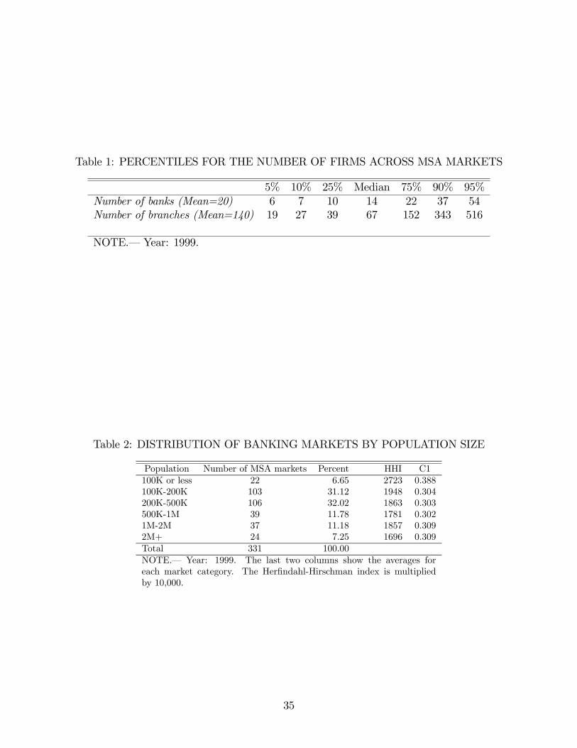
Table 1: PERCENTILES FOR THE NUMBER OF FIRMS ACROSS MSA MARKETS

5% 10% 25% Median 75% 90% 95%Number of banks (Mean=20) 6 7 10 14 22 37 54Number of branches (Mean=140) 19 27 39 67 152 343 516

NOTE.– Year: 1999.

Table 2: DISTRIBUTION OF BANKING MARKETS BY POPULATION SIZE

Population Number of MSA markets Percent HHI C1100K or less 22 6.65 2723 0.388100K-200K 103 31.12 1948 0.304200K-500K 106 32.02 1863 0.303500K-1M 39 11.78 1781 0.3021M-2M 37 11.18 1857 0.3092M+ 24 7.25 1696 0.309Total 331 100.00NOTE.– Year: 1999. The last two columns show the averages foreach market category. The Herfindahl-Hirschman index is multipliedby 10,000.

35

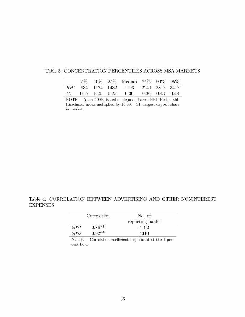
Table 3: CONCENTRATION PERCENTILES ACROSS MSA MARKETS

5% 10% 25% Median 75% 90% 95%HHI 934 1124 1432 1793 2240 2817 3417C1 0.17 0.20 0.25 0.30 0.36 0.43 0.48NOTE.– Year: 1999. Based on deposit shares. HHI: Herfindahl-Hirschman index multiplied by 10,000. C1: largest deposit sharein market.

Table 4: CORRELATION BETWEEN ADVERTISING AND OTHER NONINTERESTEXPENSES

Correlation No. ofreporting banks

2001 0.86** 41922002 0.92** 4310NOTE.– Correlation coefficients significant at the 1 per-cent l.o.c.

36

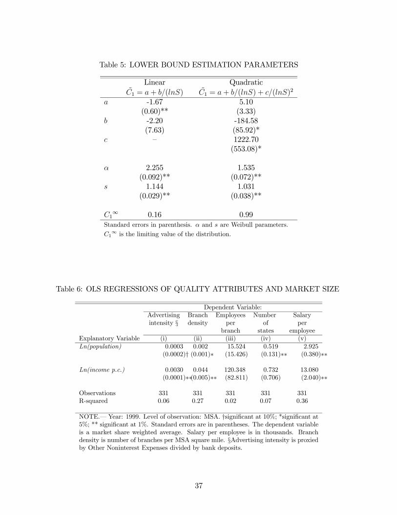
Table 5: LOWER BOUND ESTIMATION PARAMETERS

Linear QuadraticC̃1 = a+ b/(lnS) C̃1 = a+ b/(lnS) + c/(lnS)2

a -1.67 5.10(0.60)** (3.33)

b -2.20 -184.58(7.63) (85.92)*

c — 1222.70(553.08)*

α 2.255 1.535(0.092)** (0.072)**

s 1.144 1.031(0.029)** (0.038)**

C1∞ 0.16 0.99

Standard errors in parenthesis. α and s are Weibull parameters.

C1∞ is the limiting value of the distribution.

Table 6: OLS REGRESSIONS OF QUALITY ATTRIBUTES AND MARKET SIZE

Dependent Variable:Advertising Branch Employees Number Salaryintensity § density per of per

branch states employeeExplanatory Variable (i) (ii) (iii) (iv) (v)Ln(population) 0.0003 0.002 15.524 0.519 2.925

(0.0002)† (0.001)∗ (15.426) (0.131)∗∗ (0.380)∗∗

Ln(income p.c.) 0.0030 0.044 120.348 0.732 13.080(0.0001)∗∗(0.005)∗∗ (82.811) (0.706) (2.040)∗∗

Observations 331 331 331 331 331R-squared 0.06 0.27 0.02 0.07 0.36

NOTE.– Year: 1999. Level of observation: MSA. †significant at 10%; *significant at5%; ** significant at 1%. Standard errors are in parentheses. The dependent variableis a market share weighted average. Salary per employee is in thousands. Branchdensity is number of branches per MSA square mile. §Advertising intensity is proxiedby Other Noninterest Expenses divided by bank deposits.

37

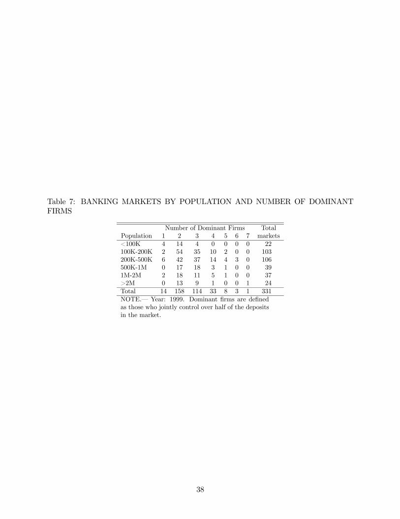
Table 7: BANKING MARKETS BY POPULATION AND NUMBER OF DOMINANTFIRMS

Number of Dominant Firms TotalPopulation 1 2 3 4 5 6 7 markets<100K 4 14 4 0 0 0 0 22100K-200K 2 54 35 10 2 0 0 103200K-500K 6 42 37 14 4 3 0 106500K-1M 0 17 18 3 1 0 0 391M-2M 2 18 11 5 1 0 0 37>2M 0 13 9 1 0 0 1 24Total 14 158 114 33 8 3 1 331NOTE.– Year: 1999. Dominant firms are definedas those who jointly control over half of the depositsin the market.

38

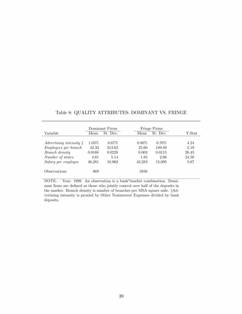
Table 8: QUALITY ATTRIBUTES: DOMINANT VS. FRINGE

Dominant Firms Fringe FirmsVariable Mean St. Dev. Mean St. Dev. T-Stat

Advertising intensity § 1.03% 0.67% 0.80% 0.70% 4.24Employees per branch 42.33 313.62 25.60 189.89 2.19Branch density 0.0168 0.0228 0.003 0.0115 26.43Number of states 4.61 5.14 1.85 2.66 24.50Salary per employee 46,281 10,962 43,283 15,095 5.67

Observations 869 5856

NOTE.– Year: 1999. An observation is a bank*market combination. Domi-nant firms are defined as those who jointly control over half of the deposits inthe market. Branch density is number of branches per MSA square mile. §Ad-vertising intensity is proxied by Other Noninterest Expenses divided by bankdeposits.

39

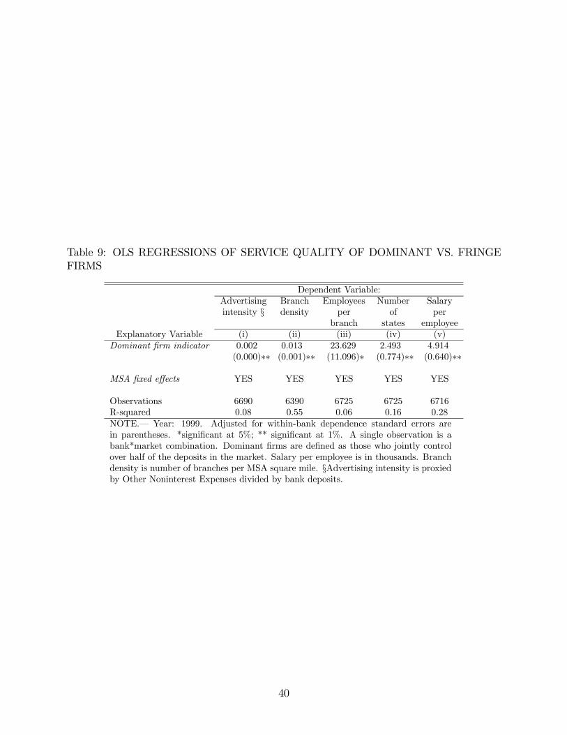
Table 9: OLS REGRESSIONS OF SERVICE QUALITY OF DOMINANT VS. FRINGEFIRMS

Dependent Variable:Advertising Branch Employees Number Salaryintensity § density per of per

branch states employeeExplanatory Variable (i) (ii) (iii) (iv) (v)Dominant firm indicator 0.002 0.013 23.629 2.493 4.914

(0.000)∗∗ (0.001)∗∗ (11.096)∗ (0.774)∗∗ (0.640)∗∗

MSA fixed effects YES YES YES YES YES

Observations 6690 6390 6725 6725 6716R-squared 0.08 0.55 0.06 0.16 0.28NOTE.– Year: 1999. Adjusted for within-bank dependence standard errors arein parentheses. *significant at 5%; ** significant at 1%. A single observation is abank*market combination. Dominant firms are defined as those who jointly controlover half of the deposits in the market. Salary per employee is in thousands. Branchdensity is number of branches per MSA square mile. §Advertising intensity is proxiedby Other Noninterest Expenses divided by bank deposits.

40

Table 10: OLS REGRESSIONS OF SERVICE QUALITY OF DOMINANT FIRMS INLARGE MSAs VS. SMALL MSAs

Dependent Variable:Advertising Branch Employees Number Salaryintensity § density per of per

branch states employeeExplanatory Variable (i) (ii) (iii) (iv) (v)

Dominant firm in large MSA 0.002 0.016 57.990 1.629 8.078(0.001)∗ (0.002)∗∗ (35.816) (0.711)∗∗ (1.212)∗∗

Observations 869 805 869 869 869R-squared 0.01 0.10 0.01 0.02 0.12NOTE.– Year: 1999. Adjusted for within-bank dependence standard errors arein parentheses. *significant at 5%; ** significant at 1%. A single observation is abank*market combination. Dominant firms are defined as those who jointly controlover half of the deposits in the market. A dominant firm in a large MSA is a dominantbank with presence in an MSA market with population greater than 500,000. Salaryper employee is in thousands. Branch density is number of branches per MSA squaremile. §Advertising intensity is proxied by Other Noninterest Expenses divided bybank deposits.

41

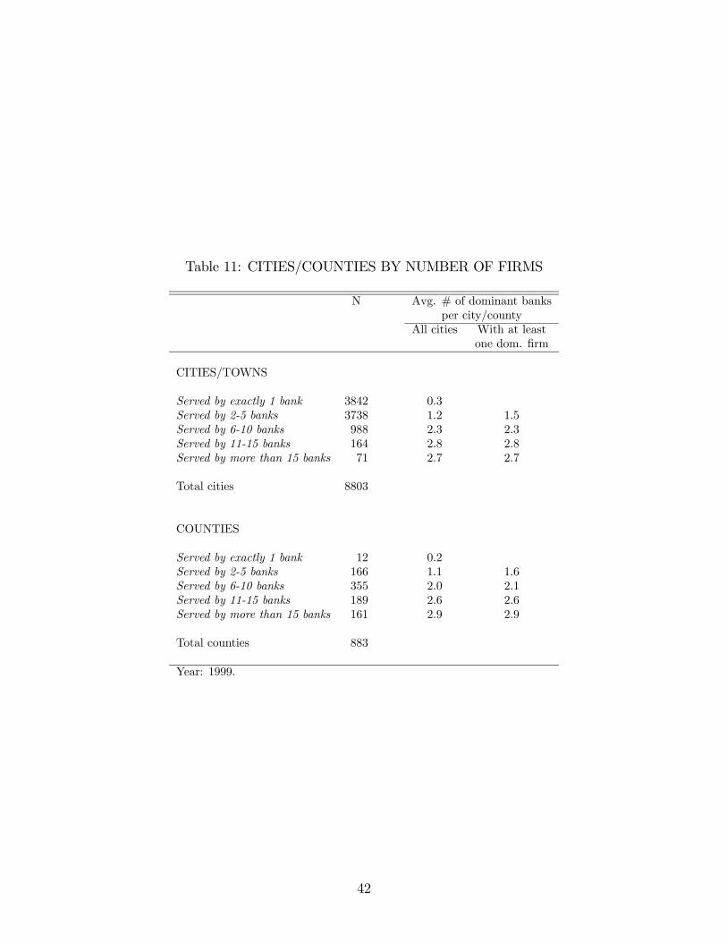
Table 11: CITIES/COUNTIES BY NUMBER OF FIRMS

N Avg. # of dominant banksper city/county

All cities With at leastone dom. firm

CITIES/TOWNS

Served by exactly 1 bank 3842 0.3Served by 2-5 banks 3738 1.2 1.5Served by 6-10 banks 988 2.3 2.3Served by 11-15 banks 164 2.8 2.8Served by more than 15 banks 71 2.7 2.7

Total cities 8803

COUNTIES

Served by exactly 1 bank 12 0.2Served by 2-5 banks 166 1.1 1.6Served by 6-10 banks 355 2.0 2.1Served by 11-15 banks 189 2.6 2.6Served by more than 15 banks 161 2.9 2.9

Total counties 883

Year: 1999.

42

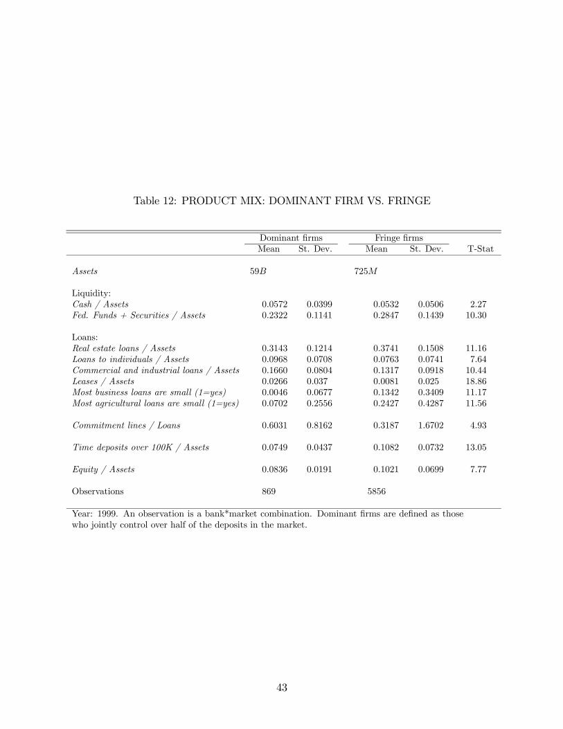
Table 12: PRODUCT MIX: DOMINANT FIRM VS. FRINGE

Dominant firms Fringe firmsMean St. Dev. Mean St. Dev. T-Stat

Assets 59B 725M

Liquidity:Cash / Assets 0.0572 0.0399 0.0532 0.0506 2.27Fed. Funds + Securities / Assets 0.2322 0.1141 0.2847 0.1439 10.30

Loans:Real estate loans / Assets 0.3143 0.1214 0.3741 0.1508 11.16Loans to individuals / Assets 0.0968 0.0708 0.0763 0.0741 7.64Commercial and industrial loans / Assets 0.1660 0.0804 0.1317 0.0918 10.44Leases / Assets 0.0266 0.037 0.0081 0.025 18.86Most business loans are small (1=yes) 0.0046 0.0677 0.1342 0.3409 11.17Most agricultural loans are small (1=yes) 0.0702 0.2556 0.2427 0.4287 11.56

Commitment lines / Loans 0.6031 0.8162 0.3187 1.6702 4.93

Time deposits over 100K / Assets 0.0749 0.0437 0.1082 0.0732 13.05

Equity / Assets 0.0836 0.0191 0.1021 0.0699 7.77

Observations 869 5856

Year: 1999. An observation is a bank*market combination. Dominant firms are defined as thosewho jointly control over half of the deposits in the market.

43

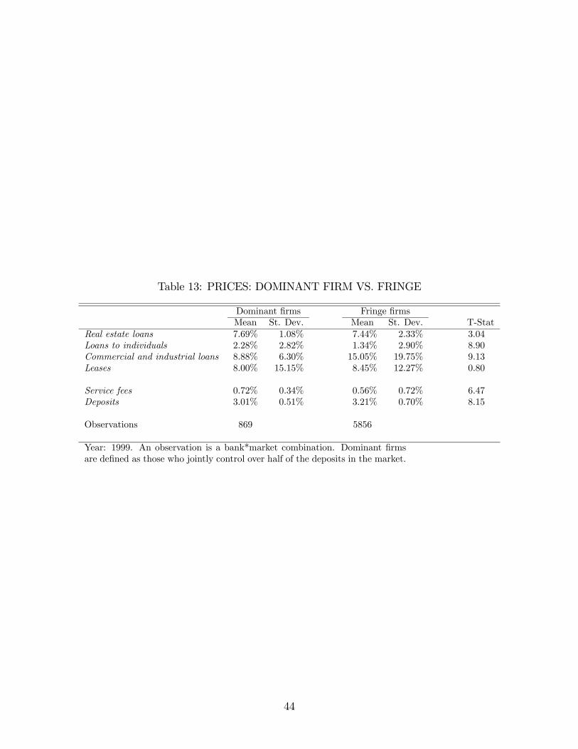
Table 13: PRICES: DOMINANT FIRM VS. FRINGE

Dominant firms Fringe firmsMean St. Dev. Mean St. Dev. T-Stat

Real estate loans 7.69% 1.08% 7.44% 2.33% 3.04Loans to individuals 2.28% 2.82% 1.34% 2.90% 8.90Commercial and industrial loans 8.88% 6.30% 15.05% 19.75% 9.13Leases 8.00% 15.15% 8.45% 12.27% 0.80

Service fees 0.72% 0.34% 0.56% 0.72% 6.47Deposits 3.01% 0.51% 3.21% 0.70% 8.15

Observations 869 5856

Year: 1999. An observation is a bank*market combination. Dominant firmsare defined as those who jointly control over half of the deposits in the market.

44

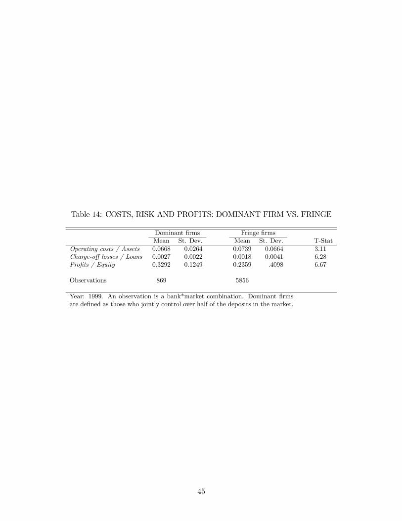
Table 14: COSTS, RISK AND PROFITS: DOMINANT FIRM VS. FRINGE

Dominant firms Fringe firmsMean St. Dev. Mean St. Dev. T-Stat

Operating costs / Assets 0.0668 0.0264 0.0739 0.0664 3.11Charge-off losses / Loans 0.0027 0.0022 0.0018 0.0041 6.28Profits / Equity 0.3292 0.1249 0.2359 .4098 6.67

Observations 869 5856

Year: 1999. An observation is a bank*market combination. Dominant firmsare defined as those who jointly control over half of the deposits in the market.

45

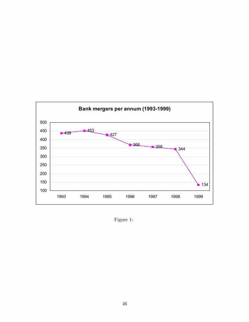
Bank mergers per annum (1993-1999)

438 453427

368 358 344

134100

150

200

250

300

350

400

450

500

1993 1994 1995 1996 1997 1998 1999

Figure 1:

46

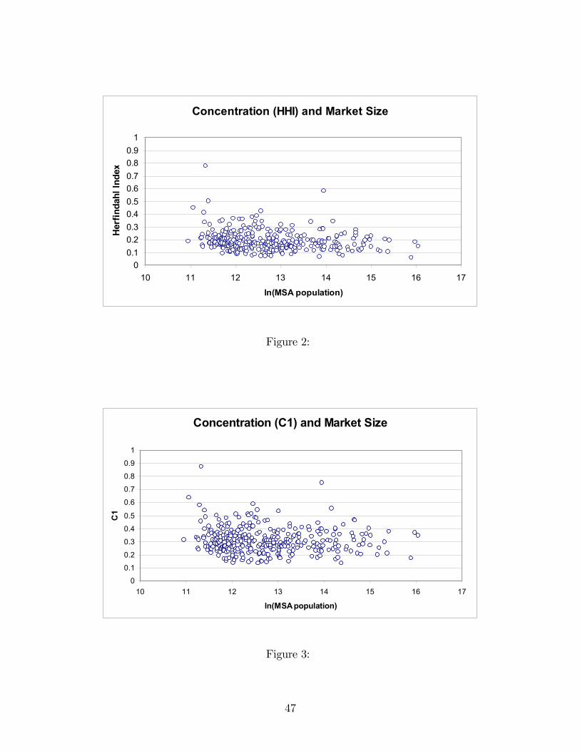
Concentration (HHI) and Market Size

00.10.20.30.40.50.60.70.80.9

1

10 11 12 13 14 15 16 17

ln(MSA population)

Her

finda

hl In

dex

Figure 2:

Concentration (C1) and Market Size

0

0.1

0.2

0.3

0.4

0.5

0.6

0.7

0.8

0.9

1

10 11 12 13 14 15 16 17

ln(MSA population)

C1

Figure 3:

47

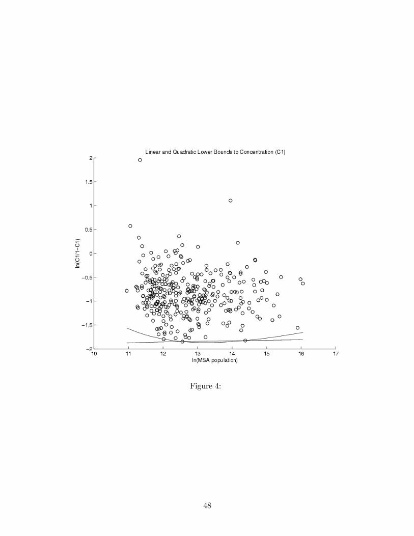
Figure 4:

48

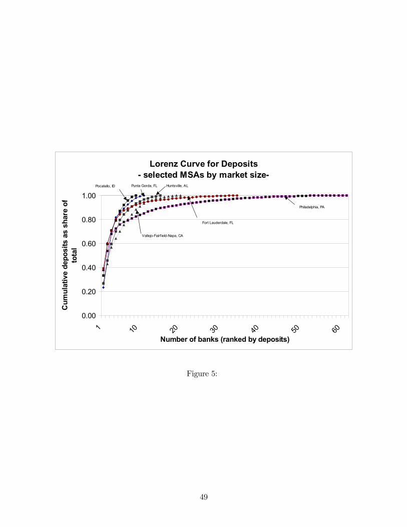
Lorenz Curve for Deposits- selected MSAs by market size-

0.00

0.20

0.40

0.60

0.80

1.00

1 10 20 30 40 50 60Number of banks (ranked by deposits)

Cum

ulat

ive

depo

sits

as

shar

e of

tota

l

Philadelphia, PA

Fort Lauderdale, FL

Vallejo-Fairf ield-Napa, CA

Pocatello, ID Punta Gorda, FL Huntsville, AL

Figure 5:

49

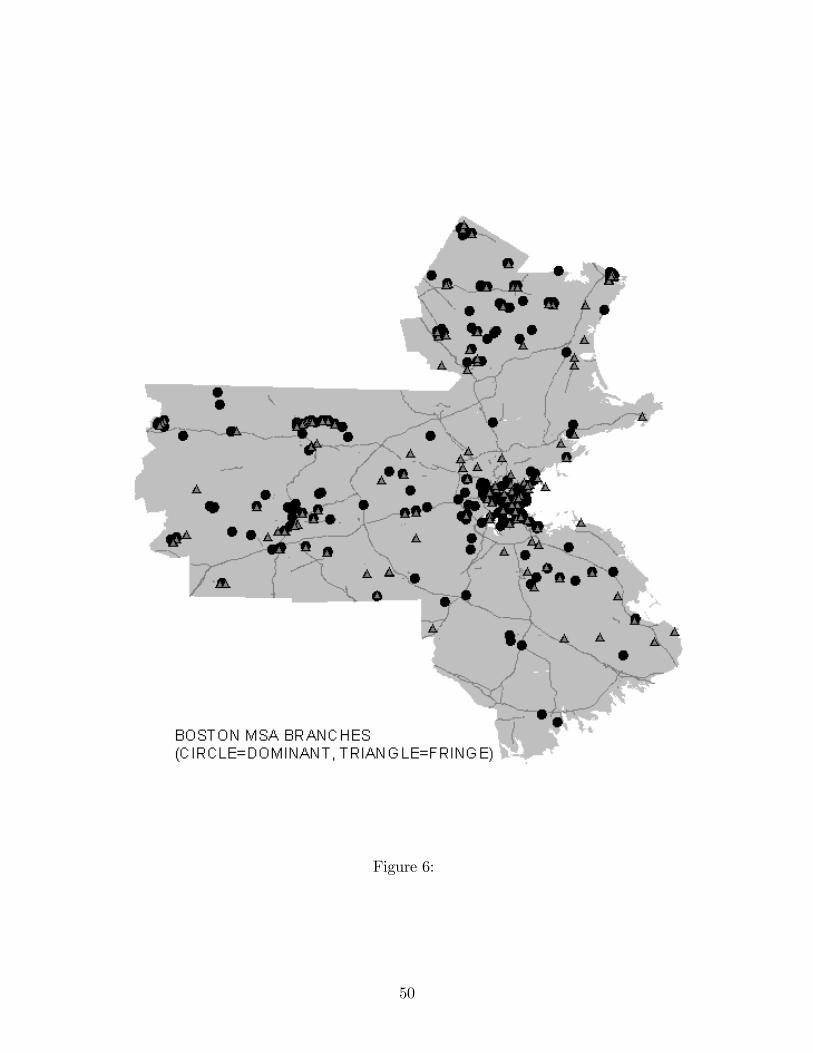
Figure 6:

50

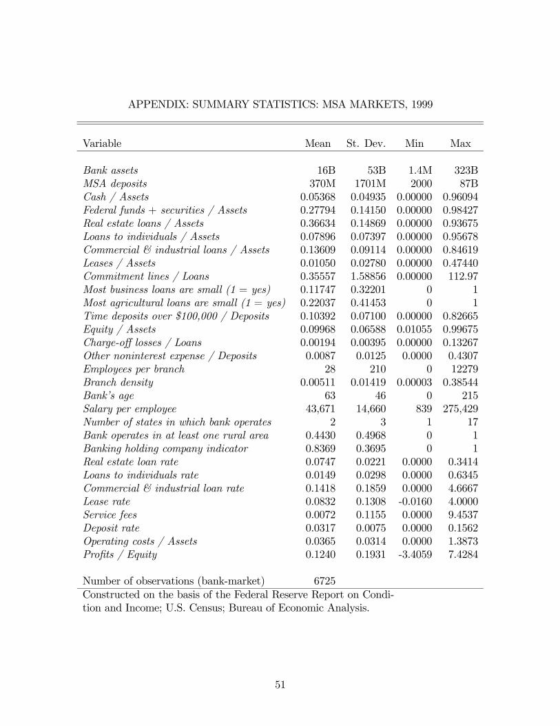
APPENDIX: SUMMARY STATISTICS: MSA MARKETS, 1999

Variable Mean St. Dev. Min Max

Bank assets 16B 53B 1.4M 323BMSA deposits 370M 1701M 2000 87BCash / Assets 0.05368 0.04935 0.00000 0.96094Federal funds + securities / Assets 0.27794 0.14150 0.00000 0.98427Real estate loans / Assets 0.36634 0.14869 0.00000 0.93675Loans to individuals / Assets 0.07896 0.07397 0.00000 0.95678Commercial & industrial loans / Assets 0.13609 0.09114 0.00000 0.84619Leases / Assets 0.01050 0.02780 0.00000 0.47440Commitment lines / Loans 0.35557 1.58856 0.00000 112.97Most business loans are small (1 = yes) 0.11747 0.32201 0 1Most agricultural loans are small (1 = yes) 0.22037 0.41453 0 1Time deposits over $100,000 / Deposits 0.10392 0.07100 0.00000 0.82665Equity / Assets 0.09968 0.06588 0.01055 0.99675Charge-off losses / Loans 0.00194 0.00395 0.00000 0.13267Other noninterest expense / Deposits 0.0087 0.0125 0.0000 0.4307Employees per branch 28 210 0 12279Branch density 0.00511 0.01419 0.00003 0.38544Bank’s age 63 46 0 215Salary per employee 43,671 14,660 839 275,429Number of states in which bank operates 2 3 1 17Bank operates in at least one rural area 0.4430 0.4968 0 1Banking holding company indicator 0.8369 0.3695 0 1Real estate loan rate 0.0747 0.0221 0.0000 0.3414Loans to individuals rate 0.0149 0.0298 0.0000 0.6345Commercial & industrial loan rate 0.1418 0.1859 0.0000 4.6667Lease rate 0.0832 0.1308 -0.0160 4.0000Service fees 0.0072 0.1155 0.0000 9.4537Deposit rate 0.0317 0.0075 0.0000 0.1562Operating costs / Assets 0.0365 0.0314 0.0000 1.3873Profits / Equity 0.1240 0.1931 -3.4059 7.4284

Number of observations (bank-market) 6725Constructed on the basis of the Federal Reserve Report on Condi-tion and Income; U.S. Census; Bureau of Economic Analysis.

51

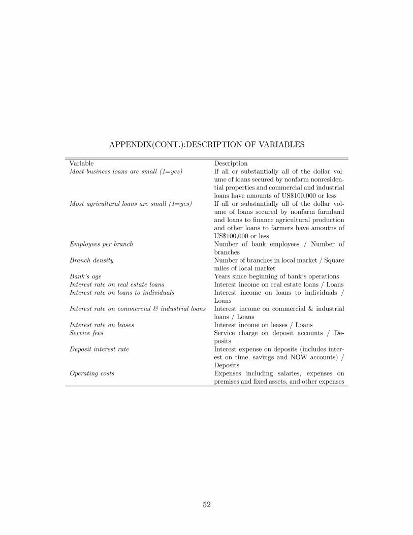
APPENDIX(CONT.):DESCRIPTION OF VARIABLES

Variable DescriptionMost business loans are small (1=yes) If all or substantially all of the dollar vol-

ume of loans secured by nonfarm nonresiden-tial properties and commercial and industrialloans have amounts of US$100,000 or less

Most agricultural loans are small (1=yes) If all or substantially all of the dollar vol-ume of loans secured by nonfarm farmlandand loans to finance agricultural productionand other loans to farmers have amoutns ofUS$100,000 or less

Employees per branch Number of bank employees / Number ofbranches

Branch density Number of branches in local market / Squaremiles of local market

Bank’s age Years since beginning of bank’s operationsInterest rate on real estate loans Interest income on real estate loans / LoansInterest rate on loans to individuals Interest income on loans to individuals /

LoansInterest rate on commercial & industrial loans Interest income on commercial & industrial

loans / LoansInterest rate on leases Interest income on leases / LoansService fees Service charge on deposit accounts / De-

positsDeposit interest rate Interest expense on deposits (includes inter-

est on time, savings and NOW accounts) /Deposits

Operating costs Expenses including salaries, expenses onpremises and fixed assets, and other expenses

52