CEP Discussion Paper No 1485 June 2017 The Key

ISSN 2042-2695

CEP Discussion Paper No 1485

June 2017

The Key Determinants of Happiness and Misery

Andrew E. Clark Sarah Flèche

Richard Layard Nattavudh Powdthavee

George Ward

Abstract Understanding the key determinants of people’s life satisfaction will suggest policies for how best to reduce misery and promote wellbeing. This paper provides evidence from survey data on USA, Australia, Britain and Indonesia, which indicate that the things that matter most are people’s social relationships and their mental and physical health. These adult factors affecting happiness are influenced in turn by the pattern of child development: the best predictor of an adult’s life satisfaction is their emotional health as a child. These results call for a new focus for public policy – not “wealth-creation” but “wellbeing-creation”.

Keywords: happiness, subjective wellbeing, life satisfaction, government, mental health

JEL codes: I31; I10

This paper was produced as part of the Centre’s Wellbeing Programme. The Centre for Economic Performance is financed by the Economic and Social Research Council.

Acknowledgements This paper was previously published in the World Happiness Report 2017. It draws heavily on the December 2016 draft of The Origins of Happiness: The Science of Wellbeing over the Life-Course by Clark et al., to be published by Princeton University Press. See also Layard et al. (2014). Support from the US National Institute on Aging (Grant R01AG040640), the John Templeton Foundation and the What Works Centre for Wellbeing is gratefully acknowledged, as is the contribution of all the survey organisations and their survey participants.

Andrew E. Clark, CNRS Research Professor, Paris School of Economics and Professorial Research Fellow, Well-Being Programme, Centre for Economic Performance, London School of Economics. Sarah Flèche, Research Economist, Well-Being Programme, Centre for Economic Performance, London School of Economics. Richard Layard, Director, Well-Being Programme, Centre for Economic Performance, London School of Economics. Nattavudh Powdthavee, Professor of Behavioural Science at Warwick Business School and Associate of the Well-Being Programme, Centre for Economic Performance, London School of Economics. George Ward, Massachusetts Institute of Technology and Associate Research Economist of the Well-Being Programme, Centre for Economic Performance, London School of Economics.

Published by Centre for Economic Performance London School of Economics and Political Science Houghton Street London WC2A 2AE

All rights reserved. No part of this publication may be reproduced, stored in a retrieval system or transmitted in any form or by any means without the prior permission in writing of the publisher nor be issued to the public or circulated in any form other than that in which it is published.

Requests for permission to reproduce any article or part of the Working Paper should be sent to the editor at the above address.

A.E. Clark, S. Flèche, R. Layard, N. Powdthavee and G. Ward, submitted 2017.

2

This paper is directed at policy-makers of all kinds – both in government and in NGOs.

We assume, like Thomas Jefferson, that “the care of human life and happiness … is the only

legitimate object of good government.”1 And we assume that NGOs would have similar

objectives. In other words, all policy-makers want to create the conditions for the greatest

possible happiness in the population and, especially, the least possible misery.

For this purpose they need to know the causes of happiness and misery. Happiness is

caused by many factors, such as income, employment, health and family life and we need to

ask, How much does a difference in each of these factors change the happiness of the person

affected?

There is also a prior and related question that tries to explain the huge variation in levels

of happiness within any country. The question is How far does the variation in each of the

factors (e.g. income inequality) explain the overall variation of happiness?

In this paper we concentrate mainly on the latter question.2 We begin by looking at the

role of current circumstances, and then (in the second part) examine the influence of earlier

childhood experience.

To be useful to policy-makers, any analysis of the causes of happiness and misery should

satisfy at least three criteria, which have not generally been satisfied in the literature.

1. It must use a consistent measure of happiness throughout.

2. It must look at the effect of all the factors affecting happiness simultaneously, not

one by one.

3. It must check whether the factors have the same effect on misery as they do on

happiness further up the scale. This is important if, as many believe, it is more

important to reduce misery than to increase happiness by an equal amount

further up the scale.

We have identified five major surveys of adults that make possible such analyses and

also include meaningful measures of mental health. They cover the USA, Australia, Britain

(two surveys) and Indonesia. We would like to have covered more countries, but the data are

not yet there.

Life satisfaction and the life-cycle

The measure of happiness that we use is life satisfaction. The typical question is “Overall

how satisfied are you with your life these days?” measured on a scale of 0 to 10 (from

‘extremely dissatisfied’ to ‘extremely satisfied’).

1 Jefferson (1809). 2 The relation between these two questions is shown in Appendix A, which provides data from which the

answers to the previous question can be calculated.

3

This is a democratic criterion – we do not rely on researchers or policy-makers to give

their own weights to enjoyment, meaning, anxiety, depression, and the like. Instead we leave

it to individuals to evaluate their own wellbeing.

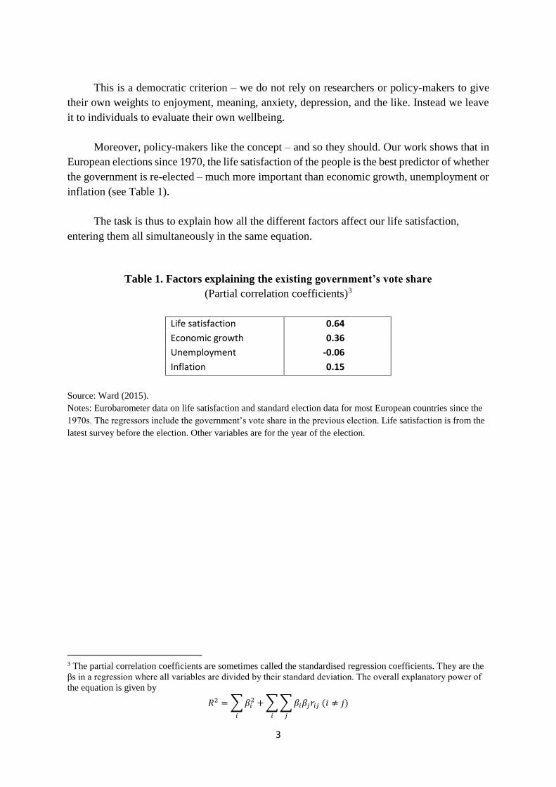
Moreover, policy-makers like the concept – and so they should. Our work shows that in

European elections since 1970, the life satisfaction of the people is the best predictor of whether

the government is re-elected – much more important than economic growth, unemployment or

inflation (see Table 1).

The task is thus to explain how all the different factors affect our life satisfaction,

entering them all simultaneously in the same equation.

Table 1. Factors explaining the existing government’s vote share

(Partial correlation coefficients)3

Life satisfaction 0.64

Economic growth 0.36

Unemployment -0.06

Inflation 0.15

Source: Ward (2015).

Notes: Eurobarometer data on life satisfaction and standard election data for most European countries since the

1970s. The regressors include the government’s vote share in the previous election. Life satisfaction is from the

latest survey before the election. Other variables are for the year of the election.

3 The partial correlation coefficients are sometimes called the standardised regression coefficients. They are the

βs in a regression where all variables are divided by their standard deviation. The overall explanatory power of

the equation is given by

𝑅2 = ∑ 𝛽𝑖2

𝑖

+ ∑ ∑ 𝛽𝑖𝛽𝑗𝑟𝑖𝑗 (𝑖 ≠ 𝑗)

𝑗𝑖

4

The life-course

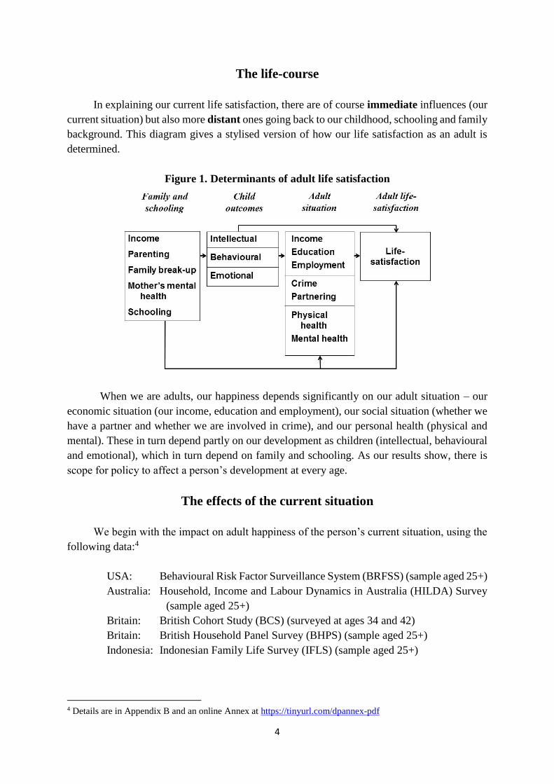
In explaining our current life satisfaction, there are of course immediate influences (our

current situation) but also more distant ones going back to our childhood, schooling and family

background. This diagram gives a stylised version of how our life satisfaction as an adult is

determined.

Figure 1. Determinants of adult life satisfaction

When we are adults, our happiness depends significantly on our adult situation – our

economic situation (our income, education and employment), our social situation (whether we

have a partner and whether we are involved in crime), and our personal health (physical and

mental). These in turn depend partly on our development as children (intellectual, behavioural

and emotional), which in turn depend on family and schooling. As our results show, there is

scope for policy to affect a person’s development at every age.

The effects of the current situation

We begin with the impact on adult happiness of the person’s current situation, using the

following data:4

USA: Behavioural Risk Factor Surveillance System (BRFSS) (sample aged 25+)

Australia: Household, Income and Labour Dynamics in Australia (HILDA) Survey

(sample aged 25+)

Britain: British Cohort Study (BCS) (surveyed at ages 34 and 42)

Britain: British Household Panel Survey (BHPS) (sample aged 25+)

Indonesia: Indonesian Family Life Survey (IFLS) (sample aged 25+)

4 Details are in Appendix B and an online Annex at https://tinyurl.com/dpannex-pdf

https://tinyurl.com/dpannex-pdf

5

The factors we examine are

Income log household income per equivalised adult

Education years, except Indonesia (higher education versus none)

Unemployment measured as ‘not unemployed’

Partnership married, or living as married

Physical health USA, Britain and Indonesia: number of illnesses; Australia:

SF36, lagged one year

Mental health USA and Australia: has ever been diagnosed for depression or an

anxiety disorder

Britain (BCS): has seen a doctor in the last year for emotional

problems

Britain (BHPS): GHQ-12, lagged one year.

Indonesia: replies to 8 questions.

Most earlier analyses of life satisfaction have not included mental health as a factor

explaining life satisfaction. The reason is that both life satisfaction and mental health are

subjective states, and there is therefore a danger that the two concepts are, at least in part,

measuring the same thing. To omit mental health as a factor in the equation, however, is to

leave out one of the most potent sources of misery, in addition to standard external causes like

poverty, unemployment, and physical illness. The solution is, whenever possible, to record

only mental illness that has been diagnosed or has led to treatment. That is our approach and it

shows clearly that mental illness not caused by poverty, unemployment or ill health is a potent

influence on life satisfaction.

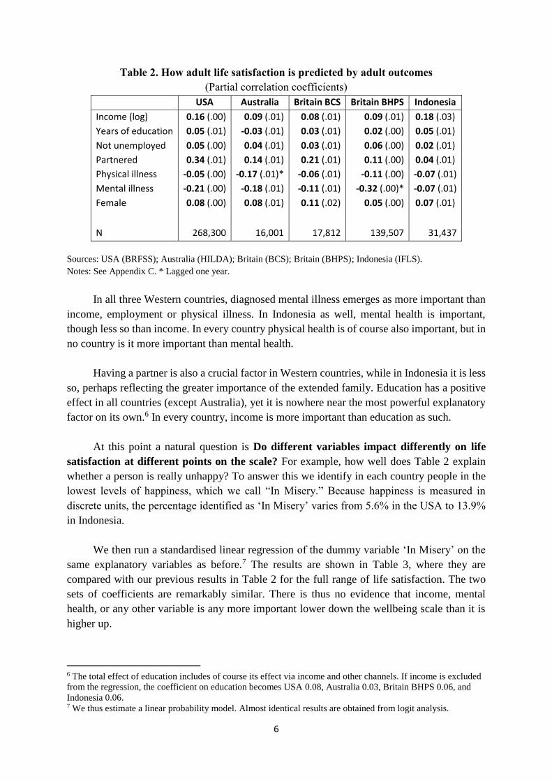
How far does each factor explain the variation in life satisfaction within the

population? Table 2 shows the results of regressing life satisfaction on all the factors

simultaneously. The coefficients given are partial correlation coefficients, which show how far

the independent variation of each factor explains the overall variation.5

5 See Note 3.

6

Table 2. How adult life satisfaction is predicted by adult outcomes

(Partial correlation coefficients)

USA Australia Britain BCS Britain BHPS Indonesia

Income (log) 0.16 (.00) 0.09 (.01) 0.08 (.01) 0.09 (.01) 0.18 (.03)

Years of education 0.05 (.01) -0.03 (.01) 0.03 (.01) 0.02 (.00) 0.05 (.01)

Not unemployed 0.05 (.00) 0.04 (.01) 0.03 (.01) 0.06 (.00) 0.02 (.01)

Partnered 0.34 (.01) 0.14 (.01) 0.21 (.01) 0.11 (.00) 0.04 (.01)

Physical illness -0.05 (.00) -0.17 (.01)* -0.06 (.01) -0.11 (.00) -0.07 (.01)

Mental illness -0.21 (.00) -0.18 (.01) -0.11 (.01) -0.32 (.00)* -0.07 (.01)

Female 0.08 (.00) 0.08 (.01) 0.11 (.02) 0.05 (.00) 0.07 (.01)

N 268,300 16,001 17,812 139,507 31,437

Sources: USA (BRFSS); Australia (HILDA); Britain (BCS); Britain (BHPS); Indonesia (IFLS).

Notes: See Appendix C. * Lagged one year.

In all three Western countries, diagnosed mental illness emerges as more important than

income, employment or physical illness. In Indonesia as well, mental health is important,

though less so than income. In every country physical health is of course also important, but in

no country is it more important than mental health.

Having a partner is also a crucial factor in Western countries, while in Indonesia it is less

so, perhaps reflecting the greater importance of the extended family. Education has a positive

effect in all countries (except Australia), yet it is nowhere near the most powerful explanatory

factor on its own.6 In every country, income is more important than education as such.

At this point a natural question is Do different variables impact differently on life

satisfaction at different points on the scale? For example, how well does Table 2 explain

whether a person is really unhappy? To answer this we identify in each country people in the

lowest levels of happiness, which we call “In Misery.” Because happiness is measured in

discrete units, the percentage identified as ‘In Misery’ varies from 5.6% in the USA to 13.9%

in Indonesia.

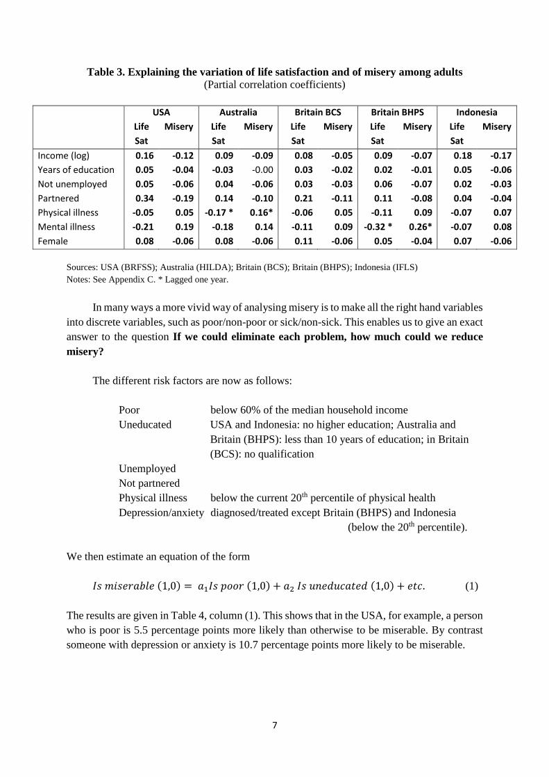
We then run a standardised linear regression of the dummy variable ‘In Misery’ on the

same explanatory variables as before.7 The results are shown in Table 3, where they are

compared with our previous results in Table 2 for the full range of life satisfaction. The two

sets of coefficients are remarkably similar. There is thus no evidence that income, mental

health, or any other variable is any more important lower down the wellbeing scale than it is

higher up.

6 The total effect of education includes of course its effect via income and other channels. If income is excluded

from the regression, the coefficient on education becomes USA 0.08, Australia 0.03, Britain BHPS 0.06, and

Indonesia 0.06. 7 We thus estimate a linear probability model. Almost identical results are obtained from logit analysis.

7

Table 3. Explaining the variation of life satisfaction and of misery among adults



Life

Sat

Misery Life

Sat

Misery Life

Sat

Misery Life

Sat

Misery Life

Sat

Misery

Income (log) 0.16 -0.12 0.09 -0.09 0.08 -0.05 0.09 -0.07 0.18 -0.17

Years of education 0.05 -0.04 -0.03 -0.00 0.03 -0.02 0.02 -0.01 0.05 -0.06

Not unemployed 0.05 -0.06 0.04 -0.06 0.03 -0.03 0.06 -0.07 0.02 -0.03

Partnered 0.34 -0.19 0.14 -0.10 0.21 -0.11 0.11 -0.08 0.04 -0.04

Physical illness -0.05 0.05 -0.17 * 0.16* -0.06 0.05 -0.11 0.09 -0.07 0.07

Mental illness -0.21 0.19 -0.18 0.14 -0.11 0.09 -0.32 * 0.26* -0.07 0.08

Female 0.08 -0.06 0.08 -0.06 0.11 -0.06 0.05 -0.04 0.07 -0.06

Sources: USA (BRFSS); Australia (HILDA); Britain (BCS); Britain (BHPS); Indonesia (IFLS)

Notes: See Appendix C. * Lagged one year.

In many ways a more vivid way of analysing misery is to make all the right hand variables

into discrete variables, such as poor/non-poor or sick/non-sick. This enables us to give an exact

answer to the question If we could eliminate each problem, how much could we reduce

misery?

The different risk factors are now as follows:

Poor below 60% of the median household income

Uneducated USA and Indonesia: no higher education; Australia and

Britain (BHPS): less than 10 years of education; in Britain

(BCS): no qualification

Unemployed

Not partnered

Physical illness below the current 20th percentile of physical health

Depression/anxiety diagnosed/treated except Britain (BHPS) and Indonesia

(below the 20th percentile).

We then estimate an equation of the form

𝐼𝑠 𝑚𝑖𝑠𝑒𝑟𝑎𝑏𝑙𝑒 (1,0) = 𝑎1𝐼𝑠 𝑝𝑜𝑜𝑟 (1,0) + 𝑎2 𝐼𝑠 𝑢𝑛𝑒𝑑𝑢𝑐𝑎𝑡𝑒𝑑 (1,0) + 𝑒𝑡𝑐. (1)

The results are given in Table 4, column (1). This shows that in the USA, for example, a person

who is poor is 5.5 percentage points more likely than otherwise to be miserable. By contrast

someone with depression or anxiety is 10.7 percentage points more likely to be miserable.

8

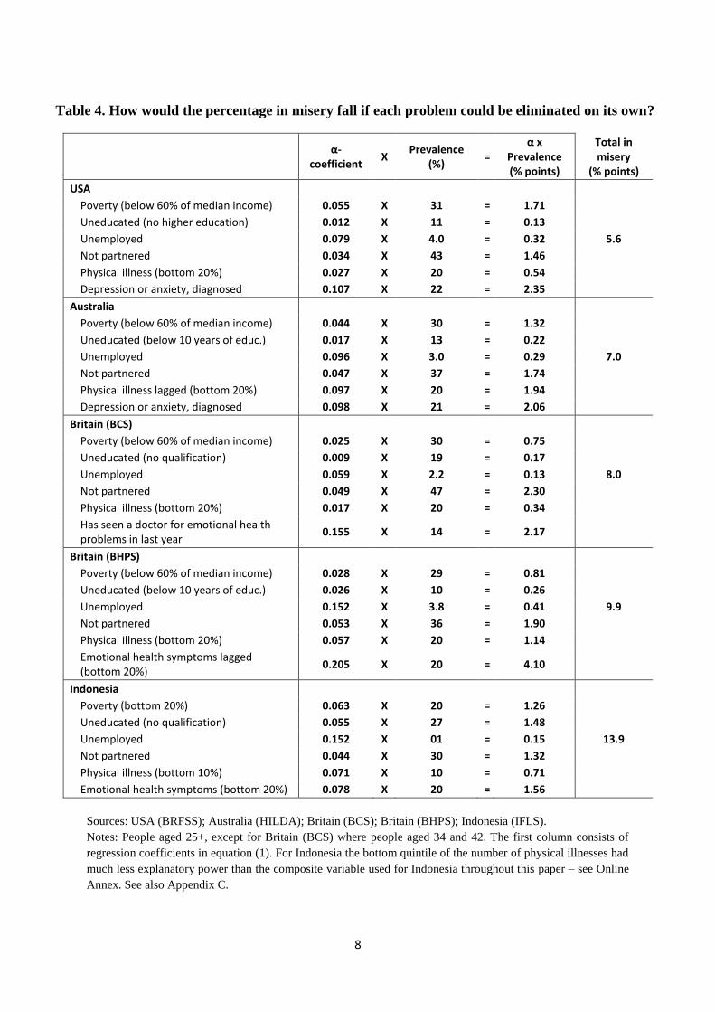
Table 4. How would the percentage in misery fall if each problem could be eliminated on its own?

α-coefficient

X Prevalence

(%) =

α x Prevalence (% points)

Total in misery

(% points)

USA

Poverty (below 60% of median income) 0.055 X 31 = 1.71

Uneducated (no higher education) 0.012 X 11 = 0.13

Unemployed 0.079 X 4.0 = 0.32 5.6

Not partnered 0.034 X 43 = 1.46

Physical illness (bottom 20%) 0.027 X 20 = 0.54

Depression or anxiety, diagnosed 0.107 X 22 = 2.35

Australia


Uneducated (below 10 years of educ.) 0.017 X 13 = 0.22

Unemployed 0.096 X 3.0 = 0.29 7.0


Physical illness lagged (bottom 20%) 0.097 X 20 = 1.94

Depression or anxiety, diagnosed 0.098 X 21 = 2.06

Britain (BCS)


Uneducated (no qualification) 0.009 X 19 = 0.17

Unemployed 0.059 X 2.2 = 0.13 8.0



Has seen a doctor for emotional health problems in last year

0.155 X 14 = 2.17

Britain (BHPS)


Uneducated (below 10 years of educ.) 0.026 X 10 = 0.26

Unemployed 0.152 X 3.8 = 0.41 9.9



Emotional health symptoms lagged (bottom 20%)

0.205 X 20 = 4.10

Indonesia

Poverty (bottom 20%) 0.063 X 20 = 1.26

Uneducated (no qualification) 0.055 X 27 = 1.48

Unemployed 0.152 X 01 = 0.15 13.9



Emotional health symptoms (bottom 20%) 0.078 X 20 = 1.56

Sources: USA (BRFSS); Australia (HILDA); Britain (BCS); Britain (BHPS); Indonesia (IFLS).

Notes: People aged 25+, except for Britain (BCS) where people aged 34 and 42. The first column consists of

regression coefficients in equation (1). For Indonesia the bottom quintile of the number of physical illnesses had

much less explanatory power than the composite variable used for Indonesia throughout this paper – see Online

Annex. See also Appendix C.

9

So how much could we reduce the prevalence of misery in the USA if we could

miraculously abolish depression and anxiety disorders without changing anything else? Well,

around 22% of the population have this diagnosis. If they were all cured, we could reduce the

percentage of the population in misery by 0.107 times 22%. This is 2.35% of the whole

population (see column 3). That is a large portion of the total 5.6% who are in misery.

By contrast, eliminating poverty in the USA reduces misery by 1.7% points,

unemployment by 0.3% and physical illness by 0.5% out of the total 5.6% in misery. Taken

together, those three factors barely make as much difference as mental illness on its own.

The pattern in Australia is very similar, but with more problems coming from physical

illness. In Britain the role of poverty is less than it is in the USA, but the role of mental health

is large or larger.

Finally in Indonesia, eliminating mental illness again reduces misery by more than

reducing poverty does. Further, increased education would also greatly help. In all countries

there would be much less misery if fewer people were living on their own.

This set of results is repeated, for effect, in Figure 3.

10

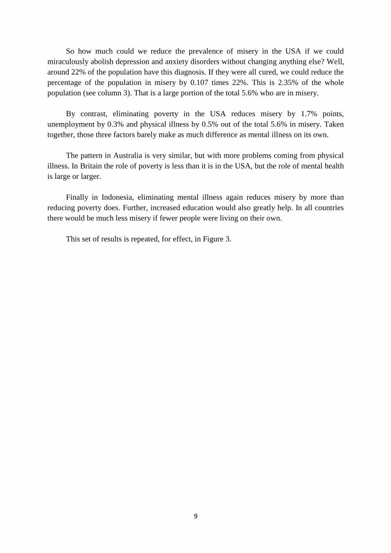
Figure 3. How would the percentage in misery fall if each problem could be eliminated on its own?

Sources: USA (BRFSS); Australia (HILDA); Britain (BHPS); Indonesia (IFLS)

From this figure we can see how much misery could be reduced if we eliminated each of

the risk factors, one at a time. But clearly none of them can be totally eliminated. Moreover the

cost of reducing them is also relevant. So a natural question to ask in each country is If we

wanted to have one less person in misery, what is the cost of achieving this by different

means? We attempt a very rough calculation of this for Britain in Table 5. As Table 5 shows,

it costs money to reduce misery, but the cheapest of the policies is treating depression and

anxiety disorders.

Table 5. Average cost of reducing the numbers in misery, by one person. Britain

£k per year

Poverty. Raising more people above the poverty line 180

Unemployment. Reducing unemployment by active labour market policy 30

Physical health. Raising more people from the worst 20% of present-day illness 100

Mental health. Treating more people for depression and anxiety 10

Sources available from authors.

11

The effects of childhood

Importantly, many of the problems of adulthood can of course be traced back to

childhood and adolescence. So which aspects of child development best predict whether an

adult is satisfied with life? Answering this question requires cohort data which are available

for many fewer countries. Since Britain is rich in such data, we shall from now on use data on

Britain only. We first use data from the British Cohort Study, which has followed children born

in 1970 right up to today.

Three key dimensions of child development are at work. One is intellectual development,

which we measure by the highest qualification that the individual achieved. This is turned into

a single variable using weights derived by regressing wages on highest qualification. A second

dimension is behavioural, measured in the Rutter behaviour questionnaire by 17 questions

answered by the mother. The third dimension is emotional health based on a malaise inventory

(22 questions answered by the child and 8 by the mother).

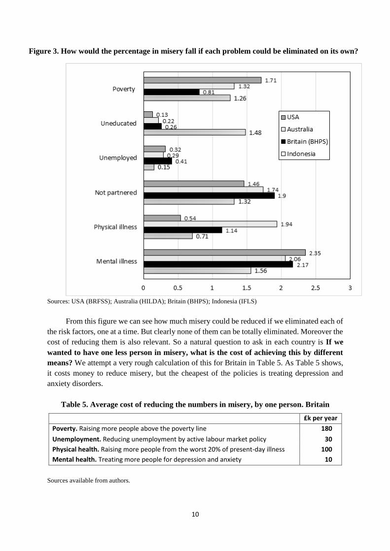
We now regress adult life satisfaction on these three variables, as well as on family

background. As Figure 4 shows, the strongest predictor of a satisfying adult life is not

qualifications but a combination of the child’s emotional health and behaviour.8 These findings

have direct relevance to policy.

Figure 4. How adults’ life satisfaction is affected by different aspects of their

development as children. Britain


Sources: Britain (BCS)

Notes: Qualifications is the highest qualification that the person achieved. Behaviour at 16 is reported by the

mother, and emotional health at 16 is reported by mother and child.

8 The coefficient for the combination of the child’s emotional health and behaviour is 0.101 (s.e. = 0.009), which

compares with 0.068 (s.e. 0.008) for qualifications – a significant difference (𝜌 = 0.010).

0 0.05 0.1 0.15

Emotional health at 16

Behaviour at 16

Qualifications

12

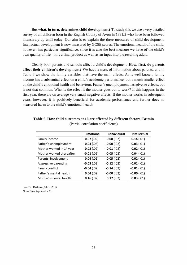
But what, in turn, determines child development? To study this we use a very detailed

survey of all children born in the English County of Avon in 1991/2 who have been followed

intensively up until today. Our aim is to explain the three measures of child development.

Intellectual development is now measured by GCSE scores. The emotional health of the child,

however, has particular significance, since it is also the best measure we have of the child’s

own quality of life – it is a final product as well as an input into the resulting adult.

Clearly both parents and schools affect a child’s development. How, first, do parents

affect their children’s development? We have a mass of information about parents, and in

Table 6 we show the family variables that have the main effects. As is well known, family

income has a substantial effect on a child’s academic performance, but a much smaller effect

on the child’s emotional health and behaviour. Father’s unemployment has adverse effects, but

is not that common. What is the effect if the mother goes out to work? If this happens in the

first year, there are on average very small negative effects. If the mother works in subsequent

years, however, it is positively beneficial for academic performance and further does no

measured harm to the child’s emotional health.

Table 6. How child outcomes at 16 are affected by different factors. Britain


Emotional Behavioural Intellectual

Family income 0.07 (.02) 0.08 (.02) 0.14 (.01)

Father’s unemployment -0.04 (.03) -0.00 (.02) -0.03 (.01)

Mother worked in 1st year -0.02 (.02) -0.01 (.02) -0.02 (.01)

Mother worked thereafter -0.01 (.02) -0.05 (.02) 0.04 (.01)

Parents’ involvement 0.04 (.02) 0.05 (.02) 0.02 (.01)

Aggressive parenting -0.03 (.02) -0.12 (.02) -0.01 (.01)

Family conflict -0.04 (.02) -0.14 (.02) -0.01 (.01)

Father’s mental health 0.04 (.02) -0.00 (.02) -0.00 (.01)

Mother’s mental health 0.16 (.02) 0.17 (.02) 0.03 (.01)

Source: Britain (ALSPAC)

Note: See Appendix C.

13

As regards “parenting style,” parental engagement and involvement with their children

(e.g. in reading and play) is immensely valuable, while aggressive parenting (hitting or

shouting) only exacerbates bad behaviour. Conflict between parents is especially

disadvantageous for the behaviour of the children. The worst thing of all for children’s

emotional health and behaviour is a mother who is mentally ill. Indeed, the survey suggests

strongly that the mother’s mental health matters more than the father’s.9

Clearly, family matters. What about the effect of schools? In the 1960s, the Coleman

Report in the US told us that parents mattered more than schools.10 Since then the tide of

opinion has turned. Our data strongly confirm the importance of the individual school and the

individual teacher. This applies equally to the academic performance of the pupils and to their

happiness.

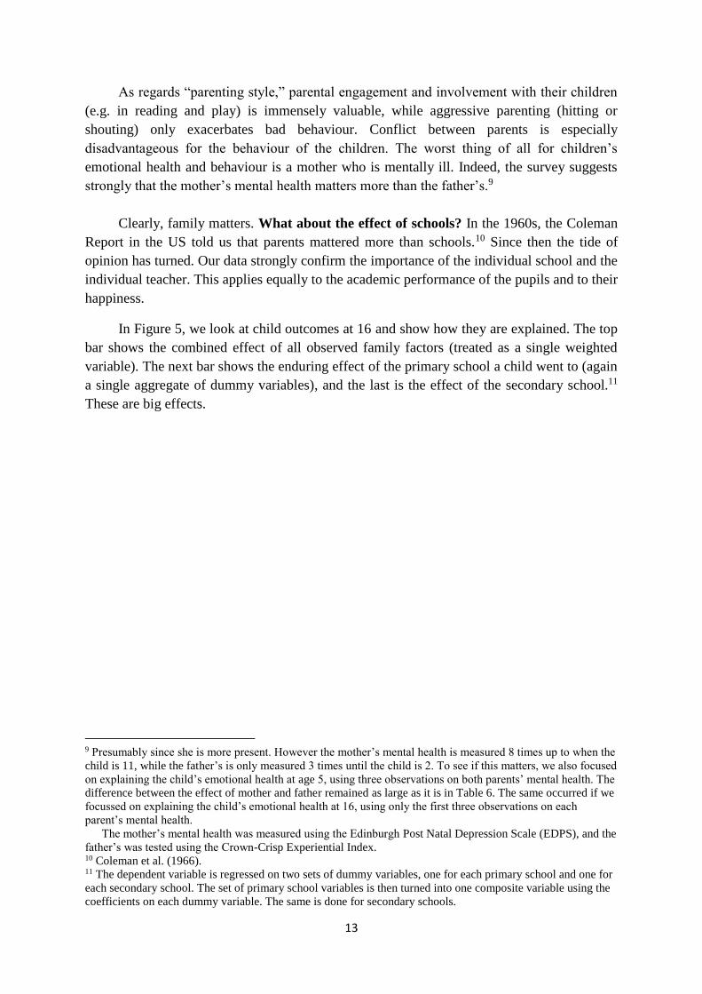
In Figure 5, we look at child outcomes at 16 and show how they are explained. The top

bar shows the combined effect of all observed family factors (treated as a single weighted

variable). The next bar shows the enduring effect of the primary school a child went to (again

a single aggregate of dummy variables), and the last is the effect of the secondary school.11

These are big effects.

9 Presumably since she is more present. However the mother’s mental health is measured 8 times up to when the

child is 11, while the father’s is only measured 3 times until the child is 2. To see if this matters, we also focused

on explaining the child’s emotional health at age 5, using three observations on both parents’ mental health. The

difference between the effect of mother and father remained as large as it is in Table 6. The same occurred if we

focussed on explaining the child’s emotional health at 16, using only the first three observations on each

parent’s mental health.

The mother’s mental health was measured using the Edinburgh Post Natal Depression Scale (EDPS), and the

father’s was tested using the Crown-Crisp Experiential Index. 10 Coleman et al. (1966). 11 The dependent variable is regressed on two sets of dummy variables, one for each primary school and one for

each secondary school. The set of primary school variables is then turned into one composite variable using the

coefficients on each dummy variable. The same is done for secondary schools.

14

Figure 5. How child outcomes at 16 are affected by family and schooling. Britain


Emotional wellbeing at 16

Behaviour at 16

Intellectual performance at 16

Source: Flèche (2017). ALSPAC data.

Notes: See Appendix C.

0 0.1 0.2 0.3 0.4

Secondary School

Primary School

Observed Family Background

0 0.1 0.2 0.3 0.4

Secondary School

Primary School


0 0.1 0.2 0.3 0.4

Secondary School

Primary School


15

Behaviour and crime

We have so far focussed exclusively on the happiness of the individual person being

studied. But each of us also has a marked impact on the happiness of other people. This social

impact has been given insufficient weight in much of the literature on happiness, although it is

well known that how others behave is a major influence on our own happiness.

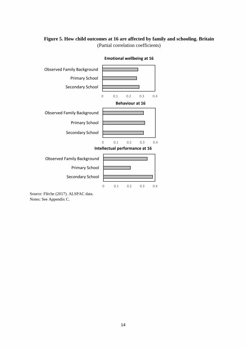
So we must modify Figure 1 to take this into account (see Figure 6). Unfortunately,

however, we have only limited ability to study this important determinant of the wellbeing of

human populations. One route is by inter-country comparisons of the type developed in Chapter

2 of the World Happiness Report 2017. The other is by studying the effects of crime on

individual happiness, and then investigating the determinants of criminality.

Figure 6. The new element: behaviour

Using data on local crime rates from police records, together with the corresponding local

happiness data from the British Household Panel Survey, we can infer that each crime on

average reduces the aggregate life satisfaction of the local population by the equivalent of 1

point-year for one person.

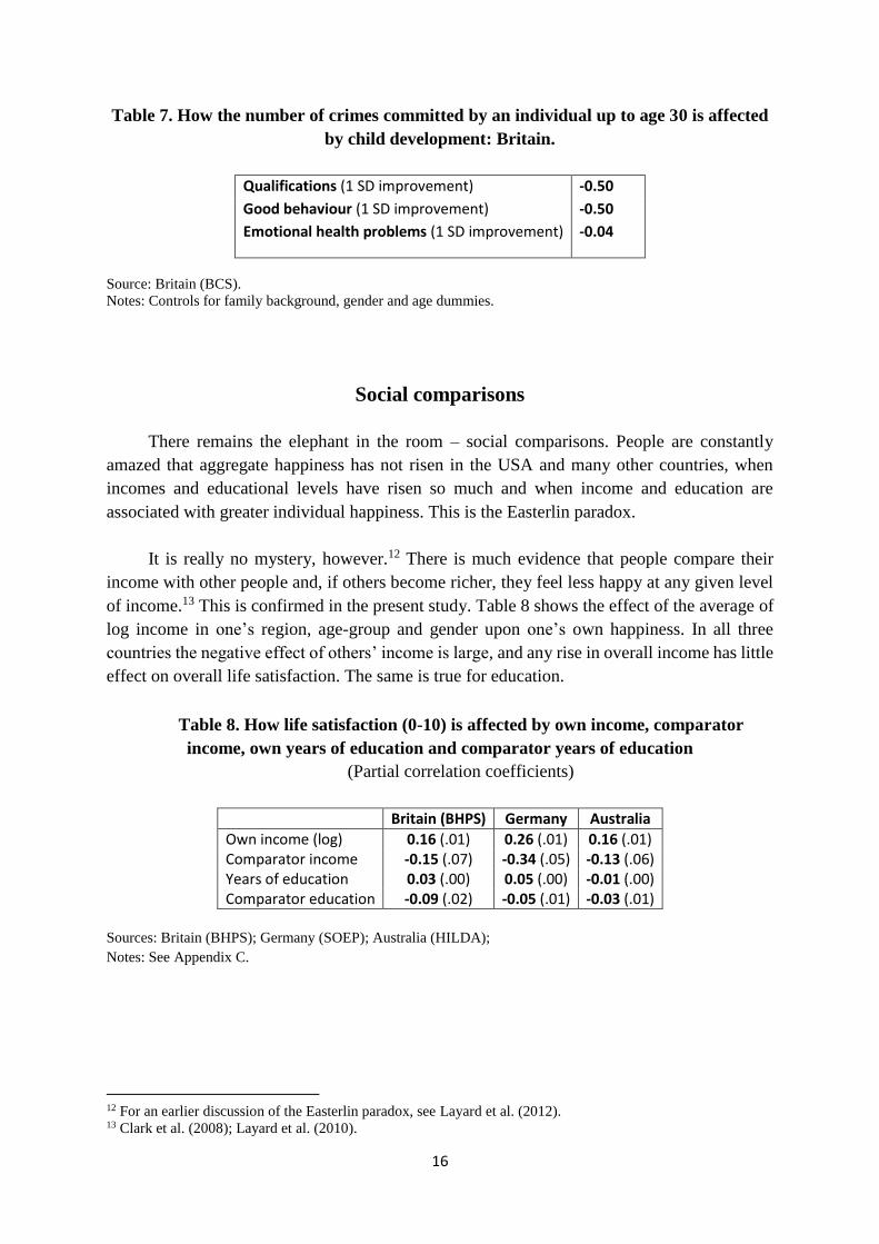
If we then look at how child development affects crime, we find that the number of crimes

a person commits is affected by child development, as shown in Table 7. Thus more education

has a major benefit through the resulting reduction of crime. From one standard deviation of

qualifications comes a one-off benefit to the rest of the population of 0.50 point-year of life

satisfaction (1 x 0.50). This can be compared to the gain to the educated individual of 0.10

point-year in every year of their life, as discussed earlier. Thus the crime-reducing effect of

education adds proportionately little to the total social returns to education.

16

Table 7. How the number of crimes committed by an individual up to age 30 is affected

by child development: Britain.

Qualifications (1 SD improvement) -0.50

Good behaviour (1 SD improvement) -0.50

Emotional health problems (1 SD improvement) -0.04

Source: Britain (BCS).

Notes: Controls for family background, gender and age dummies.

Social comparisons

There remains the elephant in the room – social comparisons. People are constantly

amazed that aggregate happiness has not risen in the USA and many other countries, when

incomes and educational levels have risen so much and when income and education are

associated with greater individual happiness. This is the Easterlin paradox.

It is really no mystery, however.12 There is much evidence that people compare their

income with other people and, if others become richer, they feel less happy at any given level

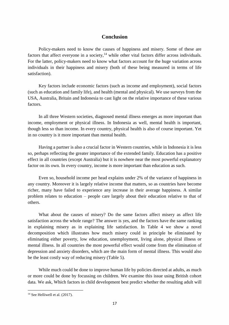
of income.13 This is confirmed in the present study. Table 8 shows the effect of the average of

log income in one’s region, age-group and gender upon one’s own happiness. In all three

countries the negative effect of others’ income is large, and any rise in overall income has little

effect on overall life satisfaction. The same is true for education.

Table 8. How life satisfaction (0-10) is affected by own income, comparator

income, own years of education and comparator years of education


Britain (BHPS) Germany Australia

Own income (log) 0.16 (.01) 0.26 (.01) 0.16 (.01) Comparator income -0.15 (.07) -0.34 (.05) -0.13 (.06) Years of education 0.03 (.00) 0.05 (.00) -0.01 (.00) Comparator education -0.09 (.02) -0.05 (.01) -0.03 (.01)

Sources: Britain (BHPS); Germany (SOEP); Australia (HILDA);

Notes: See Appendix C.

12 For an earlier discussion of the Easterlin paradox, see Layard et al. (2012). 13 Clark et al. (2008); Layard et al. (2010).

17

Conclusion

Policy-makers need to know the causes of happiness and misery. Some of these are

factors that affect everyone in a society,14 while other vital factors differ across individuals.

For the latter, policy-makers need to know what factors account for the huge variation across

individuals in their happiness and misery (both of these being measured in terms of life

satisfaction).

Key factors include economic factors (such as income and employment), social factors

(such as education and family life), and health (mental and physical). We use surveys from the

USA, Australia, Britain and Indonesia to cast light on the relative importance of these various

factors.

In all three Western societies, diagnosed mental illness emerges as more important than

income, employment or physical illness. In Indonesia as well, mental health is important,

though less so than income. In every country, physical health is also of course important. Yet

in no country is it more important than mental health.

Having a partner is also a crucial factor in Western countries, while in Indonesia it is less

so, perhaps reflecting the greater importance of the extended family. Education has a positive

effect in all countries (except Australia) but it is nowhere near the most powerful explanatory

factor on its own. In every country, income is more important than education as such.

Even so, household income per head explains under 2% of the variance of happiness in

any country. Moreover it is largely relative income that matters, so as countries have become

richer, many have failed to experience any increase in their average happiness. A similar

problem relates to education – people care largely about their education relative to that of

others.

What about the causes of misery? Do the same factors affect misery as affect life

satisfaction across the whole range? The answer is yes, and the factors have the same ranking

in explaining misery as in explaining life satisfaction. In Table 4 we show a novel

decomposition which illustrates how much misery could in principle be eliminated by

eliminating either poverty, low education, unemployment, living alone, physical illness or

mental illness. In all countries the most powerful effect would come from the elimination of

depression and anxiety disorders, which are the main form of mental illness. This would also

be the least costly way of reducing misery (Table 5).

While much could be done to improve human life by policies directed at adults, as much

or more could be done by focussing on children. We examine this issue using British cohort

data. We ask, Which factors in child development best predict whether the resulting adult will

14 See Helliwell et al. (2017).

18

have a satisfying life? We find that academic qualifications are a worse predictor than the

emotional health and behaviour of the child.

What in turn affects the emotional health and behaviour of the child? Parental income is

a good predictor of a child’s academic qualifications (as is well known), but it is a much weaker

predictor of the child’s emotional health and behaviour. The best predictor of these is the mental

health of the child’s mother.

Schools are also crucially important. Remarkably, which school a child went to (both

primary and secondary) predicts as much of how the child develops as all the characteristics

we can measure of the mother and father. This is true of what determines the child’s emotional

health, their behaviour and their academic achievement.

To conclude, within any country, mental health explains more of the variance of

happiness in Western countries than income does. In Indonesia mental illness also matters, but

less than income. Nowhere is physical illness a bigger source of misery than mental illness.

Equally, if we go back to childhood, the key factors for the future adult are the mental health

of the mother and the social ambiance of primary and secondary school. The implications for

policy are momentous.

19

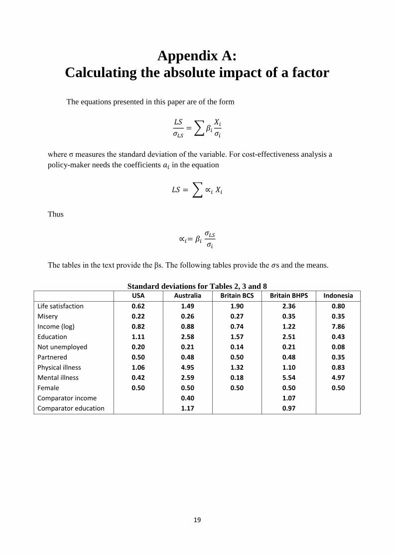
Appendix A:

Calculating the absolute impact of a factor

The equations presented in this paper are of the form

𝐿𝑆

𝜎𝐿𝑆= ∑ 𝛽𝑖

𝑋𝑖

𝜎𝑖

where σ measures the standard deviation of the variable. For cost-effectiveness analysis a

policy-maker needs the coefficients 𝑎𝑖 in the equation

𝐿𝑆 = ∑ ∝𝑖 𝑋𝑖

Thus

∝𝑖= 𝛽𝑖

𝜎𝐿𝑆

𝜎𝑖

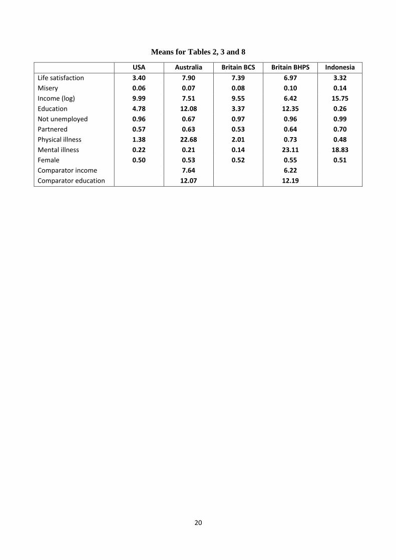
The tables in the text provide the βs. The following tables provide the 𝜎s and the means.

Standard deviations for Tables 2, 3 and 8


Life satisfaction 0.62 1.49 1.90 2.36 0.80

Misery 0.22 0.26 0.27 0.35 0.35

Income (log) 0.82 0.88 0.74 1.22 7.86

Education 1.11 2.58 1.57 2.51 0.43

Not unemployed 0.20 0.21 0.14 0.21 0.08

Partnered 0.50 0.48 0.50 0.48 0.35

Physical illness 1.06 4.95 1.32 1.10 0.83

Mental illness 0.42 2.59 0.18 5.54 4.97

Female 0.50 0.50 0.50 0.50 0.50

Comparator income 0.40 1.07

Comparator education 1.17 0.97

20

Means for Tables 2, 3 and 8


Life satisfaction 3.40 7.90 7.39 6.97 3.32

Misery 0.06 0.07 0.08 0.10 0.14

Income (log) 9.99 7.51 9.55 6.42 15.75

Education 4.78 12.08 3.37 12.35 0.26

Not unemployed 0.96 0.67 0.97 0.96 0.99

Partnered 0.57 0.63 0.53 0.64 0.70

Physical illness 1.38 22.68 2.01 0.73 0.48

Mental illness 0.22 0.21 0.14 23.11 18.83

Female 0.50 0.53 0.52 0.55 0.51

Comparator income 7.64 6.22

Comparator education 12.07 12.19

21

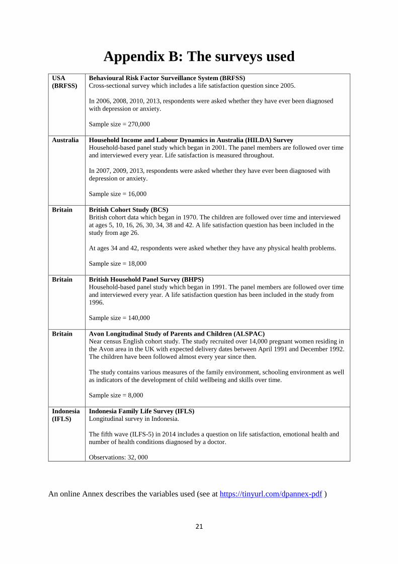
Appendix B: The surveys used

USA

(BRFSS)

Behavioural Risk Factor Surveillance System (BRFSS)

Cross-sectional survey which includes a life satisfaction question since 2005.

In 2006, 2008, 2010, 2013, respondents were asked whether they have ever been diagnosed

with depression or anxiety.

Sample size = 270,000

Australia Household Income and Labour Dynamics in Australia (HILDA) Survey

Household-based panel study which began in 2001. The panel members are followed over time

and interviewed every year. Life satisfaction is measured throughout.

In 2007, 2009, 2013, respondents were asked whether they have ever been diagnosed with

depression or anxiety.


Britain British Cohort Study (BCS)

British cohort data which began in 1970. The children are followed over time and interviewed

at ages 5, 10, 16, 26, 30, 34, 38 and 42. A life satisfaction question has been included in the

study from age 26.

At ages 34 and 42, respondents were asked whether they have any physical health problems.


Britain British Household Panel Survey (BHPS)

Household-based panel study which began in 1991. The panel members are followed over time

and interviewed every year. A life satisfaction question has been included in the study from

1996.


Britain Avon Longitudinal Study of Parents and Children (ALSPAC)

Near census English cohort study. The study recruited over 14,000 pregnant women residing in

the Avon area in the UK with expected delivery dates between April 1991 and December 1992.

The children have been followed almost every year since then.

The study contains various measures of the family environment, schooling environment as well

as indicators of the development of child wellbeing and skills over time.

Sample size = 8,000

Indonesia

(IFLS)

Indonesia Family Life Survey (IFLS)

Longitudinal survey in Indonesia.

The fifth wave (ILFS-5) in 2014 includes a question on life satisfaction, emotional health and

number of health conditions diagnosed by a doctor.

Observations: 32, 000

An online Annex describes the variables used (see at https://tinyurl.com/dpannex-pdf )

https://tinyurl.com/dpannex-pdf

22

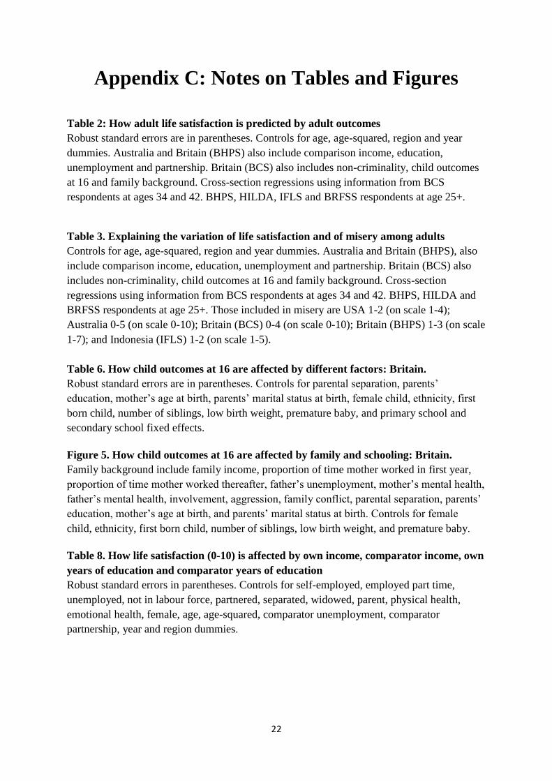
Appendix C: Notes on Tables and Figures

Table 2: How adult life satisfaction is predicted by adult outcomes

Robust standard errors are in parentheses. Controls for age, age-squared, region and year

dummies. Australia and Britain (BHPS) also include comparison income, education,

unemployment and partnership. Britain (BCS) also includes non-criminality, child outcomes

at 16 and family background. Cross-section regressions using information from BCS

respondents at ages 34 and 42. BHPS, HILDA, IFLS and BRFSS respondents at age 25+.

Table 3. Explaining the variation of life satisfaction and of misery among adults

Controls for age, age-squared, region and year dummies. Australia and Britain (BHPS), also

include comparison income, education, unemployment and partnership. Britain (BCS) also

includes non-criminality, child outcomes at 16 and family background. Cross-section

regressions using information from BCS respondents at ages 34 and 42. BHPS, HILDA and

BRFSS respondents at age 25+. Those included in misery are USA 1-2 (on scale 1-4);

Australia 0-5 (on scale 0-10); Britain (BCS) 0-4 (on scale 0-10); Britain (BHPS) 1-3 (on scale

1-7); and Indonesia (IFLS) 1-2 (on scale 1-5).

Table 6. How child outcomes at 16 are affected by different factors: Britain.

Robust standard errors are in parentheses. Controls for parental separation, parents’

education, mother’s age at birth, parents’ marital status at birth, female child, ethnicity, first

born child, number of siblings, low birth weight, premature baby, and primary school and

secondary school fixed effects.

Figure 5. How child outcomes at 16 are affected by family and schooling: Britain.

Family background include family income, proportion of time mother worked in first year,

proportion of time mother worked thereafter, father’s unemployment, mother’s mental health,

father’s mental health, involvement, aggression, family conflict, parental separation, parents’

education, mother’s age at birth, and parents’ marital status at birth. Controls for female

child, ethnicity, first born child, number of siblings, low birth weight, and premature baby.

Table 8. How life satisfaction (0-10) is affected by own income, comparator income, own

years of education and comparator years of education

Robust standard errors in parentheses. Controls for self-employed, employed part time,

unemployed, not in labour force, partnered, separated, widowed, parent, physical health,

emotional health, female, age, age-squared, comparator unemployment, comparator

partnership, year and region dummies.

23

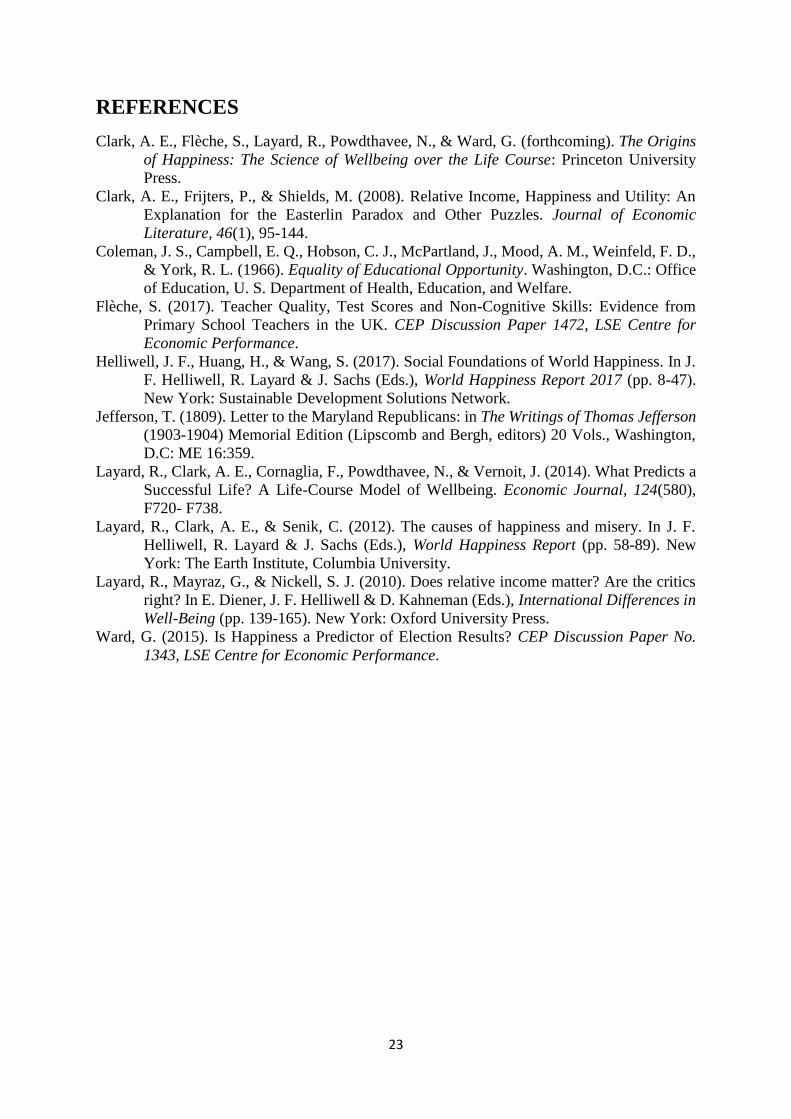
REFERENCES

Clark, A. E., Flèche, S., Layard, R., Powdthavee, N., & Ward, G. (forthcoming). The Origins

of Happiness: The Science of Wellbeing over the Life Course: Princeton University

Press.

Clark, A. E., Frijters, P., & Shields, M. (2008). Relative Income, Happiness and Utility: An

Explanation for the Easterlin Paradox and Other Puzzles. Journal of Economic

Literature, 46(1), 95-144.

Coleman, J. S., Campbell, E. Q., Hobson, C. J., McPartland, J., Mood, A. M., Weinfeld, F. D.,

& York, R. L. (1966). Equality of Educational Opportunity. Washington, D.C.: Office

of Education, U. S. Department of Health, Education, and Welfare.

Flèche, S. (2017). Teacher Quality, Test Scores and Non-Cognitive Skills: Evidence from

Primary School Teachers in the UK. CEP Discussion Paper 1472, LSE Centre for

Economic Performance.

Helliwell, J. F., Huang, H., & Wang, S. (2017). Social Foundations of World Happiness. In J.

F. Helliwell, R. Layard & J. Sachs (Eds.), World Happiness Report 2017 (pp. 8-47).

New York: Sustainable Development Solutions Network.

Jefferson, T. (1809). Letter to the Maryland Republicans: in The Writings of Thomas Jefferson

(1903-1904) Memorial Edition (Lipscomb and Bergh, editors) 20 Vols., Washington,

D.C: ME 16:359.

Layard, R., Clark, A. E., Cornaglia, F., Powdthavee, N., & Vernoit, J. (2014). What Predicts a

Successful Life? A Life-Course Model of Wellbeing. Economic Journal, 124(580),

F720- F738.

Layard, R., Clark, A. E., & Senik, C. (2012). The causes of happiness and misery. In J. F.

Helliwell, R. Layard & J. Sachs (Eds.), World Happiness Report (pp. 58-89). New

York: The Earth Institute, Columbia University.

Layard, R., Mayraz, G., & Nickell, S. J. (2010). Does relative income matter? Are the critics

right? In E. Diener, J. F. Helliwell & D. Kahneman (Eds.), International Differences in

Well-Being (pp. 139-165). New York: Oxford University Press.

Ward, G. (2015). Is Happiness a Predictor of Election Results? CEP Discussion Paper No.

1343, LSE Centre for Economic Performance.

CENTRE FOR ECONOMIC PERFORMANCE Recent Discussion Papers

1484 Matthew Skellern The Hospital as a Multi-Product Firm: The Effect of Hospital Competition on Value-Added Indicators of Clinical Quality

1483 Davide Cantoni Jeremiah Dittmar Noam Yuchtman

Reallocation and Secularization: The Economic Consequences of the Protestant Reformation

1482 David Autor David Dorn Lawrence F. Katz Christina Patterson John Van Reenen

The Fall of the Labor Share and the Rise of Superstar Firms

1481 Irene Sanchez Arjona Ester Faia Gianmarco Ottaviano

International Expansion and Riskiness of Banks

1480 Sascha O. Becker Thiemo Fetzer Dennis Novy

Who voted for Brexit? A Comprehensive District-Level Analysis

1479 Philippe Aghion Nicholas Bloom Brian Lucking Raffaella Sadun John Van Reenen

Turbulence, Firm Decentralization and Growth in Bad Times

1478 Swati Dhingra Hanwei Huang Gianmarco I. P. Ottaviano João Paulo Pessoa Thomas Sampson John Van Reenen

The Costs and Benefits of Leaving the EU: Trade Effects

1477 Marco Bertoni Stephen Gibbons Olmo Silva

What’s in a name? Expectations, heuristics and choice during a period of radical school reform

1476 David Autor David Dorn Lawrence F. Katz Christina Patterson John Van Reenen

Concentrating on the Fall of the Labor Share

1475 Ruben Durante Paolo Pinotti Andrea Tesei

The Political Legacy of Entertainment TV

1474 Jan-Emmanuel De Neve George Ward

Happiness at Work

1473 Diego Battiston Jordi Blanes i Vidal Tom Kirchmaier

Is Distance Dead? Face-to-Face Communication and Productivity in Teams

1472 Sarah Flèche Teacher Quality, Test Scores and Non-Cognitive Skills: Evidence from Primary School Teachers in the UK

1471 Ester Faia Gianmarco Ottaviano

Global Banking: Risk Taking and Competition

1470 Nicholas Bloom Erik Brynjolfsson Lucia Foster Ron Jarmin Megha Patnaik Itay Saporta-Eksten John Van Reenen

What Drives Differences in Management?

1469 Kalina Manova Zhihong Yu

Multi-Product Firms and Product Quality

1468 Jo Blanden Kirstine Hansen Sandra McNally

Quality in Early Years Settings and Children’s School Achievement

1467 Joan Costa-Font Sarah Flèche

Parental Sleep and Employment: Evidence from a British Cohort Study

1466 Jo Blanden Stephen Machin

Home Ownership and Social Mobility

The Centre for Economic Performance Publications Unit Tel: +44 (0)20 7955 7673 Email [email protected] Website: http://cep.lse.ac.uk Twitter: @CEP_LSE

mailto:[email protected]

http://cep.lse.ac.uk/

Documents

CEP Discussion Paper No 1485 June 2017 The Key