ISSN 2042-2695

CEP Discussion Paper No 1640

August 2019

Innovation Union: Costs and Benefits of

Innovation Policy Coordination

Teodora Borota

Fabrice Defever

Giammario Impullitti

Abstract In this paper, we document large heterogeneity in innovation policy and performance between old and new

EU member states, and present firm-level evidence on the close link between foreign direct investment (FDI) spillovers and eastern European _firms' innovation. Guided by these facts and motivated by the pressing debate on further EU integration, we build a two-region endogenous growth model to analyse the gains from innovation policy cooperation in an economic union. The two regions, the West (the old members) and the East (the new post-2004 members), feature firms competing in innovation for market leadership, are integrated via free trade and costly technology transfer via FDI and have different

innovation performance and policy. Calibrating the model to reproduce key features of the EU economy, we compare the outcomes of an East-West R&D subsidy war with a cooperation scenario with unified subsidy across regions, and obtain three main results. First, we find that the dynamic gains spurring from the impact of cooperation on the economy's growth rate are sizable and substantially larger than the static gains obtained internalising the strategic motive for subsidies. Second, our model suggests that the presence of FDI and multinational production alleviates the strategic motive and increases the gains from

cooperation. Third, separating FDI and innovation policy generates larger gains from cooperation, a policy complementarity driven by the knowledge spillovers carried by FDI. Key words: Optimal innovation policy, growth theory, international policy coordination, EU integration,

FDI spillovers. JEL Codes: O41, O31, O38, F12, F42 F43

This paper was produced as part of the Centre’s Trade Programme. The Centre for Economic Performance

is financed by the Economic and Social Research Council.

We want to thank Ufuk Akcigit, Omar Licandro, Kalina Manova, Andres Rodriguez-Clare and seminar

participants at Central Bank of Serbia, College de France, European Commission DG Industry, LSE,

Queen Mary, Stockholm School of Economics (SITE) and Sveriges Riskbank for comments and

suggestions. Impullitti thanks the British Academy for financial support.

Teodora Borota, Uppsala University. Fabrice Defever, City University of London and Centre for

Economic Performance, London School of Economics. Giammario Impullitti, University of Nottingham

and Centre for Economic Performance, London School of Economics.

Published by

Centre for Economic Performance

London School of Economics and Political Science

Houghton Street

London WC2A 2AE

All rights reserved. No part of this publication may be reproduced, stored in a retrieval system or

transmitted in any form or by any means without the prior permission in writing of the publisher nor be

issued to the public or circulated in any form other than that in which it is published.

Requests for permission to reproduce any article or part of the Working Paper should be sent to the editor

at the above address.

T. Borota, F. Defever and G. Impulllitti, submitted 2019.

1 Introduction

The recent financial crises have increased the demand for stronger international economic policy

coordination on the one hand, and triggered movements toward more policy independence on

the other. While some European countries are promoting an ‘ever closer union’ agenda of further

policy coordination, in a historical referendum the UK voted to terminate its EU membership.

While there is sufficient consensus that trade integration should not be reversed, less agreement

can be found on the virtues of coordination in other areas such as banking, fiscal and innovation

policies. In the aftermath of the 2008 financial crisis, the debate on the completion of Europe’s

Economic and Monetary Union (EMU) intensified around the needs and the breadth of future

fiscal and banking union (Berger et al., 2018).

In 2010, the EU launched the Innovation Union, a flagship initiative of the Europe 2020

strategy. An ambitious and wide plan spanning from the creation of a single market for inno-

vation via, for example, the introduction of the Unitary Patent, a procedure aimed at radically

cutting the bureaucratic cost of patenting in the EU, to a strong financial support of innova-

tive firms, grant/subsidies for innovative small-medium enterprises (SME instruments) and a

specific innovation procurement budget (European Commission, 2015). Moreover, the recent

Commission’s proposal of a plan for a Common, Consolidated, Corporate Tax Base, which

includes an R&D incentive, can be seen as a first step toward a unified tax treatment of R&D

(d’Andria et al., 2017). These and other Commission’s initiatives can be interpreted as an

initial plan to move toward some degree of unification of innovation policy.

Motivated by these political and institutional developments, this paper provides a macroe-

conomic framework to evaluate the effects of tax and direct government support for innovation

and assess the costs and benefits of policy coordination in an economic union. One fundamental

task in exploring these issues is to identify the key structural difference between countries and

understand their role in shaping the aggregate effects of policy coordination and their distribu-

tion across regions. Another important task for the analysis of optimal policies is to identify

the externalities that the policy tools are set forth to tackle.

We document large differences between EU members in innovation performances and in

innovation policy. These differences are especially pronounced when comparing the new member

states (NMS), the eastern European countries that entered with the enlargement started in 2004,

and the Old Members, all western European countries. In the period 2008-16, business R&D as

a share of GDP is on average 1.31% in western EU countries and 0.5% in eastern countries. The

employment share of scientists and engineers in manufacturing is 7.2% on average in the West

and 4.2% in the East. An even more striking picture can be obtained looking at innovation

output, with over 97% of the patents granted by the European Patent Office (EPO) assigned to a

western European firm. Although the differences are still large, some non-negligible innovation

dynamism can be observed in eastern Europe: the business R&D share of GDP has almost

1

doubled between 2008 and 2016 and similar patterns can be observed in the employment share

of scientists and engineers and in the EPO patent share.

Along with the recent surge in innovation in the NMS of the EU, we observe a similarly

strong increase in inward foreign direct investment. The stock of FDI was about 30% of the

total NMS GDP before their entry into the EU and it grew to 70% a decade later, most of

it coming from the old EU members. Using firm-level data from the Business Environment

and Enterprise Performance Survey (BEEPS) we provide new evidence linking the dynamic

innovation performance in NMS, and in other Central and East European Countries, with the

surge in FDI and foreign firms’ presence. Finally, we document the wide heterogeneity in both

government funding of business R&D and indirect support via tax incentives, both between old

and new members and within each group.

Guided by these facts and motivated by the recent EU plans to increase innovation policy

coordination we set up a two-region, West-East, Schumpetarian growth model of an economic

union where trade is free and firms compete in innovation for market leadership. Western firms

invest in quality-improving innovation to gain market leadership, once successful they can

decide to produce in the high-wage West or incur an adaptive R&D, or FDI, cost to transfer

the technology and produce in the low-wage East. Transferring the technology abroad generates

local knowledge spillovers which allow eastern firms to start innovating and potentially replace

western market leaders. Hence, two opposite forces drive FDI: the labor cost difference between

East and West, the wage gap, and the difference in Schumpeterian ‘creative destruction’ in the

two regions, the creative destruction gap. The higher the innovation in the West compared to

the East in a given industry, the lower is the risk for a western firm of losing market leadership

when transferring production abroad. Market leadership and production can switch back to

the West if one of its firms succeeds in innovating.1 Innovation in the West and in the East

drives the long-run growth rate of the economy which, in the absence of trade costs, is the same

for both regions. Adaptive R&D spending has only indirect effects on growth, allowing eastern

firms to innovate.

In our benchmark model, we consider one type of policy, R&D subsidies directed to both

innovation and adaptive R&D spending (FDI). The reasons for subsidising or taxing R&D in

our economy are related to the classical spillovers of Schumpeterian growth models (Aghion

and Howitt, 1992, and Grossman and Helpman, 1991b) plus some additional elements related

to the open economy and multinational production. When an innovation arrives it benefits

consumers immediately, via the higher quality of the good, we dub this the consumer surplus

effect, but also in the future as future innovations build on past innovations, the intertemporal

spillovers or growth effect. These effects are not taken into account by innovating firms, thereby

1The product cycle in each industry occurs in three stages: first through western FDI to the East, then bythe eastern innovation to win the sectoral leadership, and finally through leapfrogging of the West which returnsthe sector’s production location to the West.

2

motivating subsidies to R&D. Moreover, when a firm successfully innovates in a product line,

it drives the incumbent firm out of the market. Appropriating the incumbent firm’s monopoly

profits, the innovating firm reduces the income of the households owning those firms, thereby

reducing aggregate consumption which, in turn, lowers the profits of the other leading firms.

The innovating firm does not take this into account and is therefore bound to overinvest in

R&D. This business-stealing effect is a motive for taxing innovation.

In open economy the business stealing produced by innovation can also shift profits and

jobs/wages across borders, from foreign firms and workers to their domestic counterparts. This

international business-stealing effect (IBSE henceforth) represents a strategic motive for coun-

tries to subsidise their firms’ R&D (Spencer and Brander, 1983, Eaton and Grossman, 1986).

The possibility of offshoring production tames this motive for subsidies. Higher innovation in

the West increases the West-East creative destruction gap, thereby increasing the incentives

for FDI. More production transfer implies a shift in labor demand and, in same specifications

of the model, partially in profits to the East thereby triggering an adverse profit and wage-

shifting effect hurting the West. Higher innovation in the East instead, decreases the creative

destruction gap, thereby reducing production transfer from the West. Lower FDI implies lower

wages and profits in the East and therefore lower incentives to subsidise eastern R&D. Hence,

higher integration via production offshoring weakens the strategic motive for subsidies.

We calibrate the model to aggregate and sectorial data to reproduce key facts of the EU

economy, which we divide in two regions: the old members, the West in the model, and the

new members, the East in the model, which are the eastern European countries that entered

after 2004. We first compute the Nash equilibrium R&D subsidies, obtained assuming that the

two regions set them non-cooperatively, maximising their own welfare. Second, we calculate a

unified subsidy chosen by a EU-level policy maker to maximise the total Union welfare. We

find the Nash subsidies to be positive and substantially above those observed in the data.

This suggests that the real economy features a substantial underinvestment in innovation, and

that the market economy in the model underinvests as well. The domestic business-stealing

effect, the externality supporting R&D taxes is weaker than the consumer surplus effect, the

growth effect and the strategic motive, the external effects of innovation supporting subsidies.

In setting the unified subsidy, the EU-level policy maker internalises the strategic motive, the

international business-stealing effect, taking into account the profit and wage shifting role of

subsidies. The planner also internalises the effect of each country’s subsidy on the other country

consumer surplus and growth. We find that the optimal unified subsidy is substantially larger

than the Nash subsidy, which suggests that the internalisation of the consumer surplus and the

growth effect of innovation are the key driver of R&D policy cooperation.

The welfare gains from a unique EU R&D subsidy are quite large but not equally distributed.

Moving from the observed subsidies to the optimal unified subsidy yields a 12% increase in

long-run consumption. While the unified subsidy generates a 5.7% gains compared to the non-

3

cooperative subsidies. The dynamic gains spurring from the impact of policy cooperation on the

economy’s growth rate are substantially larger than the static gains obtainable by internalising

consumer surplus and business-stealing effects. Hence, the knowledge externality typical of

Schumpeterian models, and the driver of long-run growth in most endogenous growth models,

proves to be the key force shaping the gains from R&D policy cooperation.

The gains from cooperation are concentrated in the East while the West does not experience

any significant improvement. Since trade is free, internalising the consumer surplus and the

growth effect benefits both countries equally. Internalising the international business stealing

effect, instead, has unequal welfare implications. In the Nash scenario, the West leads in almost

all sectors of the economy, either via direct leadership or via multinationals. Hence, the incen-

tives to cooperate to contain East business stealing are quite low. In parametrisations where

the innovation asymmetries between the two regions are smaller, the incentives to cooperate

for the West are larger.

FDI alleviates the strategic motive for subsidies and increases the gains from policy coop-

eration. We show this by increasing the exogenous efficiency of the adaptive R&D technology

which leads to more production offshoring. When the regions are more integrated, the rewards

for a subsidy war are lower as business stealing is less effective and, consequently, the optimal

Nash subsidies are lower as well. The unified subsidy, on the other hand, increases when FDI

is more efficient. More FDI leads to more technology transfer and more knowledge spillovers

to the East, allowing eastern firms to innovate more efficiently and in more sectors. These

stronger external effects on eastern firms are not taken into account in the FDI decisions of

western firms, hence there is a stronger reason for the EU-level policy maker to set higher subsi-

dies to internalise them. Consequently, the larger gains from cooperation arise from a stronger

need to internalise the growth effect of subsidies in economies that are more integrated via FDI.

Finally, our benchmark economy bundles together an innovation policy, the R&D subsidy,

and an FDI subsidy, which can be seen as a more standard trade policy, as it affects the cost of

multinational activity with no direct implications for innovation. In an extension, we consider

the subsidy to FDI and the subsidy to R&D separately and quantify the specific gains produced

by optimal cooperative innovation and FDI policy. The overall gains from policy cooperation

over Nash are now higher than in the baseline scenario. The gains from innovation policy alone

are similar to the total gains obtained in the benchmark model, 5.2% of consumption equivalent,

but the optimal FDI policy generates an additional 3.2% gains. The complementarity between

FDI and R&D subsidies produces the larger gains from cooperation: more FDI leads to stronger

international knowledge spillovers which, in turn, strengthen the growth effect on innovation

subsidies.

Literature review. The paper is related to several strands of the literature. First, the

strategic motive for subsidies has been widely studied in the strategic trade and industrial

4

policy literature. Contributions focusing on R&D subsidies are the pioneering Spencer and

Brander (1983), the following work by Leahy and Neary (1997, 2009) and Haaland and Kind

(2008) among others. Papers analysing the strategic role of trade policy include Eaton and

Grossman (1986), Maggi (1996), and more recent contributions by Felbermayr et al. (2013)

and Campolmi et al. (2018). In a sequence of recent papers Ossa (2011, 2014, 2015) revisits

the key questions in the literature with a modern quantitative approach. Our contribution to

this line of work is to cast the analysis in a dynamic framework and show that the impact

of innovation policies on productivity growth are quantitatively relevant for the gains from

cooperation.2 This results echoes the recent finding in the trade and growth literature showing

that the dynamic gains from trade-induced selection magnifies the gains obtainable in static

models with firm heterogeneity (Sampson, 2016, Impullitti and Licandro, 2018, Perla et al.,

2015). We extend this result to the gains from policy cooperation and, in addition, we explore

the role of multinationals in shaping these gains.

A second related literature is the recent body of quantitative work on the effects of R&D

subsidies in closed economy models of endogenous growth, such as Acemoglu and Akcigit (2012),

Acemoglu et al. (2018), Akcigit et al. (2016) among others. Open economy applications include

Impullitti (2010) and Akcigit et al. (2018), which present quantitative evaluations of the US

R&D subsidy policy in the 1980s and 1990s. We follow a similar approach and we contribute

focusing on the analysis of the strategic policy and the gains from cooperation, and introducing

multinational corporations.

We make contact with a few recent papers analysing FDI and innovation jointly. Arkolakis

et al. (2018) build a quantitative model of trade and multinational production in which countries

may specialise in innovation and relegate production to other countries via offshoring. They

use the model to analyse the effects of changes in FDI costs. Acemoglu et al. (2015) analyse

the effects of changes in offshoring costs on technical change and wage inequality in a Ricar-

dian model with multinationals and endogenous technical change. Dinopoulos and Segerstrom

(2010) introduce offshoring in a North-South Schumpeterian growth model to study the effects

of an increase in the protection of international property rights on innovation and the wage

gap between countries. We draw on Dinopoulos and Segerstrom’s modeling strategy but al-

low the firms in the South (the East in our model) to innovate and not simply exogenously

imitate northern technology. We present a quantitative analysis, focus on R&D subsidies and

analyse the strategic policy interaction between countries and the cost and benefits from policy

cooperation.3

2Grossman and Lai (2004) and Kondo (2013) explore the gain from intellectual property rights policy coop-eration in endogenous growth models. We complement their theoretical analysis with a quantitative approach,focusing on R&D subsidies, and exploring the role of multinationals.

3Segerstrom and Jakobsson (2017) present a dynamic product-cycle model of North-South trade with multi-national production to perform a quantitative analysis of the TRIPS agreements for developing countries butabstract from strategic policy interactions.

5

Finally, our paper touches upon the empirical literature analysing the link between FDI

and innovation. This literature recognises that FDI may act as a vehicle of technology transfer.

Local firms may imitate technological innovations introduced by affiliates of multinational firms

(Blomstrom and Kokko, 1997). Another major channel of knowledge diffusion may arise when

inventors move from subsidiaries of foreign firm to newly started spin-outs. In this case, new

entrepreneurs build on knowledge learned when working for their previous employers. According

to Audretsch and Feldman (2003), spin-out is one of the most important mechanisms through

which knowledge is transmitted locally. Finally, positive productivity spillovers from FDI may

take place through backward and forward linkages between foreign affiliates and local firms

(Javorcik, 2004).

The evidence on productivity spillovers of FDI though remains mixed (e.g. Gorg and Green-

away, 2014), while recent papers have provided robust evidence of FDI spillovers on domestic

firms’ innovation. Gorodnichenko et al. (2010) and Gorodnichenko et al. (2015) document

strong positive spillover effects from FDI on innovation by domestic firms in Eastern and

Central European countries using firm-level data on innovation activity, such as the devel-

opment of new products or the adoption of new technologies. This empirical evidence is in

line with our theoretical model where the establishment of a foreign subsidiary is necessary for

the domestically-owned firms to be able to learn the western technology and start innovating

upon it. We provide additional evidence showing that the link between FDI and innovation in

Eastern European economies is robust to several model specifications.

The rest of the paper is organised as follows: sections 2 presents some stylised facts on

R&D policy and innovation in EU states and provides empirical evidence on the link between

FDI and innovation. Section 3 presents the model, while the quantitative analysis and the key

results are shown in Section 4. Section 5, analyses the robustness of the results to changes in

some key parameters and presents some extensions of the main model. Section 6 concludes.

2 Motivating Facts

We present a set of descriptive statistics providing motivation for our modelling strategy and

empirical support for the quantitative analysis. We document a large heterogeneity in inno-

vation activities and innovation policy across European countries. Moreover, we identify a

strong relationship between the presence of western multinationals and the innovation activity

performed by local firms in eastern European countries .

2.1 Innovation performance and policy support.

While innovation in Europe is still concentrated in the West, a growing and non-negligible

share is performed in the new member states (NMS). Figures 1 and 2 illustrate the differences

6

in innovation efforts for the year 2008 and 2016 between the old (West) and the new (East)

members that have joined the European-Union in May 2004 onwards.4 Business R&D as a

share of GDP is substantially higher in western compared to eastern EU countries, with an

average of 1.31% for the former and 0.5% for the latter in the period 2008-16.5 However,

several East EU countries, such as Slovenia, the Czech Republic, Hungary, Estonia and Poland

show non-negligible and increasing R&D intensity outperforming quite a few old EU members.

A similar picture can be obtained looking at the employment share of scientists and engineers

in manufacturing. In the period 2008-16, 7.2% of employment in the West was accounted for

by scientists and engineers (S&E), while in the East the share is 4.2%. Moreover, the S&E

employment share increases in this period in several eastern countries.

Figure 1: Business Enterprise R&D Expenditure (% of GDP)

0

0.5

1

1.5

2

2.5

3

OLD MEMBERS (WEST) NEW MEMBERS (EAST)

2016

2008

Source: Eurostat.

Governments can choose among various instruments to promote business R&D, either by

providing direct support, such as grants, contracts, loans and subsidies, or through indirect

support, such as tax allowances, credits, and accelerated depreciation of R&D capital expendi-

tures. The absence of a common EU innovation policy translates in a strong heterogeneity in

the public support for innovation. As an illustration, Figure 3 provides the direct and indirect

(tax credit) government R&D support in 2012 as a percentage of the countries’ GDP by the

4The old members are Germany, France, Italy, the Netherlands, Belgium, Luxembourg, Denmark, Ireland,United Kingdom, Greece, Spain, Portugal, Austria, Finland and Sweden. The new members are Czech Republic,Cyprus, Estonia, Latvia, Lithuania, Hungary, Malta, Poland, Slovenia and Slovakia that joined in 2004, Romaniaand Bulgaria, joined in 2007 and Croatia in 2013.

5The average difference between East and West is smaller if we consider total R&D, which includes publicinvestment. The West records an average of 2% while the East attains a 0.9%.

7

Figure 2: Scientists and Engineers (% of employment in manufacturing sector)

0

2

4

6

8

10

12

14

16

18

OLD MEMBERS (WEST) NEW MEMBERS (EAST)

2008

2016

Source: Eurostat.

new and old member states’ governments. France and Slovenia provide the most combined

R&D funding for business as a percentage of GDP, with more than 0.35 percent of their GDP

spent on R&D support. There are striking disparities in both direct and indirect (tax credit)

support both for the old and the new member states. Of our sample of 22 countries, all the 16

western EU countries and the 6 new EU members received “direct” government support. In

addition, 11 of the 16 old EU members and 3 of the 6 new EU members give “indirect” R&D

support, such as tax credit. On average West EU governments provide direct support to R&D

corresponding to about 0.08% of GDP and indirect support through the tax system of a similar

amount. In the East, the direct support is larger (about 0.12% of GDP on average) and the

indirect incentives amount to 0.03% of GDP.

This set of descriptive statistics deliver two clear messages. First, there is a large hetero-

geneity in innovation performances across EU countries with most of the activity concentrated

in the Northern and old member countries. The amount of innovation performed in the new

member countries is, though, substantial and growing. Second, the absence of a common EU

innovation policy produces a strong heterogeneity in the public support for innovation.

2.2 Western multinationals and innovation in the East

Along with the increase in innovation, we observe a marked increase in inward FDI in the new

member states. FDI stock as a share of total GDP of NMS doubles between 2001 and 2012. Over

this period, the share of FDI stock in the NMS accounted for by the old members remains large

8

Figure 3: Direct government funding and Indirect government support through tax incentives,2012

BERD: business enterprise expenditure on R&D. Source: OECD R&D Tax IncentivesIndicators.

and stable around 80% (Eurostat). We dig deeper into the potential relationship between FDI

and innovation analysing the empirical link between the presence of multinational affiliates and

the local innovation activity of domestic firms. To this end, we rely on the Business Environment

and Enterprise Performance Survey (BEEPS) which provides self-reported information from top

managers on various types of innovation activity. This firm-level survey based on face-to-face

interviews with managers realised during the years 2011-2014, includes 15,694 firms located in

Eastern and Central European countries, as well as Russia and Turkey. For those years, the

data provide information on the 2-digit sector classification, the exact regional location as well

as the ownership of each firm.

An additional key feature of the BEEPS survey is that it includes several questions on

product and process innovation. Firms report the introduction of the following innovation in

the last 3 years: i) New products or services ii) New production or supply methods iii) New

organisational, management practices or structures iv) New marketing methods. Based on

this information, we identify domestic firms which report at least one of these new product or

process innovations in a given year.6 This direct firm-level measure of innovation has previously

been used by Gorodnichenko et al. (2010) and Gorodnichenko et al. (2015).7

6As the BEEPS survey only reports the number of firms reporting at least one new product or innovationover a 3 year period, we use the binomial distribution formula to recover the probability for a firm to reportone additional product in a given year.

7While most studies on innovation use patent data or R&D expenditures, these authors argue that thesemeasures are potentially problematic. Patents are likely to capture inventions rather than innovations, while

9

Aggregate results. We make use of this information to aggregate the data at the region-

sector level and calculate both the share of domestic firms conducting innovation as well as the

fraction of firms with foreign capital.8 We furthermore exclude all region-sector pair with fewer

than 10 active firms.9 Using two-way clustering, we report robust standard error clustered

both at the regional and at the sector level. We regress the share of domestically-owned firms

reporting innovations on the share of firms with foreign capital in Table 1. We do that without

any additional control in column 1. We then introduce region fixed-effects in column 2 and

sector fixed-effects in column 3. In all regressions, we find a positive and significant relationship

at the 1% level between the share of domestically-owned firms reporting innovations and the

share of foreign affiliates. The positive relationship is also robust to the inclusion of both set of

fixed-effects simultaneously, as in column 4. While the size of the coefficient largely decreases,

it remains significant at the 1% level. Raising the share of foreign affiliates from the 25th to

the 75th percentile (that is from 0 to 0.083) is associated with a predicted change in the share

of domestic firms reporting innovation by 3.3 percentage points.

Table 1: Aggregate results: Share of Domestic firms reporting innovation and share of foreignfirms at the region-sector level

Dependent variable:Share of domestic firms reporting innovation at the region-sector level

(1) (2) (3) (4)Share of foreign affiliates 0.701*** 0.422*** 0.660*** 0.401***

(0.133) (0.124) (0.127) (0.120)region fixed-effects No Yes No YesSector fixed-effects No No Yes YesObservations 346 346 346 346R-squared 0.140 0.817 0.169 0.835

Robust standard error clustered both at the region and at the sectorlevel into brackets. *, **, *** significantly different from 0 at 10%, 5%and 1% level, respectively.

Firm-level results. We then turn to a firm-level linear-probability model. Focusing on

domestic firms, we construct our dependent variable as a dummy variable taking a value one

if the firm reports product or process innovations, and zero otherwise. We then construct our

main explanatory variable in two different ways: as a dummy variable indicating the presence or

not of a foreign firm within the same region and within the same 2-digit sector than the firm, or

R&D does not necessarily lead to innovation.8We consider as a foreign affiliate a firm with at least 50 percent of the capital owned by a foreign en-

trepreneur/company.9Increasing the threshold to 20 or 30 active firms would decrease the number of observations but leads to

qualitatively similar results.

10

as the count of foreign firms within the same sector-location. Table 2 reports our main results

where all estimations include region, sector and year fixed effects. Regressions (2) and (4) also

include additional firm-level controls: firms’ log of sales and a set of dummy variables for state-

owned enterprises, exporting and importing status. The coefficient associated with ‘foreign

presence’ is significant at least at the 5% level in all the estimations. Considering Column (2),

a foreign presence in a region-sector is associated with an increase by 3.5 percentage points of

the predicted probability for a domestic firm to report innovation.10 In the appendix, we also

split the sample in many different ways and, as reported in Table A.1, we find more pronounced

effects in manufacturing sectors than in services, and for private firms compared to state-owned

enterprises. Effects also appear independent of the export and import status of the firm and

persistent both for small and large firms (below or above the median size).

Table 2: Firm-level evidence: Domestic firms reporting innovation and foreign presence

Dependent variable:Firm-level dummy variable for domestic firms reporting innovationExplanatory variable: dummy dummy count count

(1) (2) (3) (4)Foreign presence 0.034** 0.035*** 0.014*** 0.012***

(0.014) (0.013) (0.003) (0.003)Control variables No Yes No YesObservations 14,877 11,466 14,877 11,466R-squared 0.167 0.209 0.168 0.209

All regressions include region, sector and year fixed effects. Regressions(2) and (4) include the following firm-level control variables: firms’ logof sales, and a set of dummy variables for state-owned enterprises, ex-porting firms, importing firms. Robust standard error clustered both atthe region and at the sector level into brackets. *, **, *** significantlydifferent from 0 at 10%, 5% and 1% level, respectively.

While the literature on technology transfer recognises that FDI may act as a vehicle of

technological transfer and may facilitate innovation in receiving countries, our suggestive ev-

idence do not imply causation. Nevertheless, our results highlight the geographic clustering

of domestic innovative firms in sectors with active foreign affiliates. Our findings complement

those obtained by Gorodnichenko et al. (2010) and Gorodnichenko et al. (2015) using similar

data for the same set of countries, but for different period of time.11 While they use firm-level

sales to multinational affiliates to identify vertical linkages between domestic firms and foreign

10Furthermore excluding all region-sector pair with fewer than 10 or 20 active firms as in the aggregateestimations would generate qualitatively similar results with similar sizable effects.

11The information on the exact region of location of firms is only available for the years 2011-2014. Unfortu-nately, the information on the firm-level sales to multinational firms used by Gorodnichenko et al. (2010) andGorodnichenko et al. (2015) is not available for those years.

11

affiliates, we use a more general definition capturing the presence of foreign affiliates within the

same region-sector.

3 The Model

We consider an economy consisting of two regions: the old members (the West) including

the developed high-wage economies, and the new members (the East) which consists of new

lower-wage EU member countries. Labor in the West is employed in two types of activities:

manufacturing of goods and innovative R&D which results in a quality upgrade of the goods.

The West can hire labor in the East to conduct adaptive R&D in order to transfer production

to the low-wage East. We call those firms western multinational enterprise subsidiaries, or the

MNEs. The adaptive R&D spending can be regarded as FDI that facilitate technology and

production transfer. Even when financed by eastern savings, as in our main specification, its

intensity is still decided by the West and a fraction of the subsidiaries’ higher global profits get

repatriated back to the consumers in the West in the form of royalties.

While the West is capable of conducting innovation in all sectors of the economy, the East

faces technological constraints and is able to innovate only in those sectors where previous

western FDI has occurred. We view this feature of the model as a way to represent the

importance of FDI knowledge spillovers which facilitate learning and the innovative activity of

the East. Once a successful quality innovation in the East has occurred, the East takes over

the global leadership in the sector until leapfrogged again by the western innovators. Trade

between the two regions is free and the product cycle within a sector occurs in three stages:

first through western FDI in the East, then by the eastern upgrade of the product quality to

obtain the sectoral leadership, and finally through leapfrogging of the West which returns the

sector’s production to the West.

3.1 Households

Consider a two-region economy, East and West, in which households have the same intertempo-

raly additively separable preferences over an infinite set of sectors indexed by ω ∈ [0, 1]. Each

household is endowed with a unit of labor time whose supply generates no disutility. Dropping

region indexes for notation simplicity, households choose their optimal consumption bundle for

each date by solving the following optimization problem:

maxU =

∫ ∞0

L0e−(ρ−n)t log u(t)dt (1)

subject to

12

u(t) ≡(∫ 1

0

jmax(ω,t)∑j=0

λj(ω,t)d(j, ω, t)

σ−1σ

dω

) σσ−1

c(t) ≡∫ 1

0

jmax(ω,t)∑j=0

p(j, ω, t)d(j, ω, t)

dωW (0) + Z(0)−

∫ ∞0

L0e−

∫ t0 (r(s)−n)dsτdt =

∫ ∞0

L0e−

∫ t0 (r(s)−n)dsc(t)dt,

where L0 is the initial population and n is its constant growth rate, ρ is the common rate of

time preference - with ρ > n - and r(t) is the market interest rate on a risk-free bond available

in both regions. d(j, ω, t) is the per-member flow of goods in sector ω, each good of quality

level j ∈ {0, 1, 2, ...}, purchased by a household at time t ≥ 0. p(j, ω, t) is the price of a good of

quality level j in sector ω at time t, c(t) is nominal expenditure, and W (0) and Z(0) are human

and non-human wealth levels. A new vintage of a good ω yields a quality equal to λ times the

quality of the previous vintage, with λ > 1. jmax(ω, t) denotes the maximum quality in which

the good in sector ω is available at time t. As is common in quality ladder models we will

assume price competition at all dates, which implies that in equilibrium only the top quality

product is produced and consumed in positive amounts. Finally, τ is a per-capita lump-sum

tax.

The instantaneous utility function is a quality-augmented CES consumption index, with

σ > 1. Households maximise static utility by spreading their expenditures c(t) across the

product linez and purchasing in each line only the product with the lowest price per unit of

quality, that is the product of quality level j = jmax(ω, t). Hence, the household’s demand of

each product is:

d(ω, t) = q(ω, t)p(ω, t)−σc(t)

P (t)1−σ , (2)

where q(ω, t) = λj(ω,t)(σ−1) is a measure of the good’s quality and P (t) =[ ∫ 1

0q(ω, t)p(ω, t)1−σdω

] 11−σ

is the quality-price index. The presence of a lump sum tax does not change the standard solu-

tion of the intertemporal maximization problem, which leads to the standard Euler equation,

·c

c= r(t)− ρ. (3)

We focus on the analysis of the steady state equilibrium where per capita expenditure c is

constant and therefore r(t) = r = ρ.

13

3.2 Product market

In each region, firms can hire workers to produce any consumption good ω ∈ [0, 1] using a linear

technology with unit labor requirement ak, where k = W,E,M is the producer indicator for

the West, the East and the western multinational subsidiary respectively. The wage rate in the

two regions is wK , K = W,E. In each industry the top quality product can be manufactured

only by the firm that has discovered it, as patent rights are protected by a perfectly enforceable

world-wide patent law. As is usual in Schumpeterian models with vertical innovation (e.g.

Grossman and Helpman, 1991b and Aghion and Howitt, 1992), firms conduct R&D activity

to improve their good’s quality and obtain market leadership. The innovation size is fixed

at λ > 1, so that when an innovation arrives λ measures the quality gap between the leader

and the follower. The patent system grants the quality leader a temporary monopoly which is

destroyed when the firm is leapfrogged by the next innovator.

Assumption 1. Trade is free in the economic union.

Since our quantitative application will be to the EU, it is natural to assume away any tariffs,

export subsidies or other political barriers to trade. Our analysis focuses on R&D subsidies

and FDI costs/barriers so we also assume away any other form of trade costs.12 We restrict our

attention to the steady state equilibria where the following conditions are satisfied: wE > aWwW

aEλ,

wE > aWwW

aMλand λ > aE

aM. These conditions guarantee the existence of a complete product cycle.

The first condition states that the innovation quality improvement is large enough for a western

quality leader producing in the West to have a lower quality-adjusted production cost than an

eastern firm producing in the east one step below on the quality ladder. If wages are lower in

the East this condition suggests the western quality leader can drive the lower cost competitor

out of the market. Similarly the second condition posits that a western quality leader can

outcompete a foreign affiliate producing a quality inferior good at a lower unit cost. The third

condition states that the quality jump is large enough to allow the eastern innovator to leapfrog

the western multinational.

We follow the common practice and assume that to participate in pricing competition, in

each product line, firms must pay a small fee (e.g. Howitt, 1999, Dinopoulos and Segerstrom,

2010). Under this assumption the profit maximising choice of the quality leader is always to

charge the monopoly price:13

pK(ω, t) =σ

σ − 1aKwK(t). (4)

12Other, non policy-related, trade costs could be easily added but are not key for the questions we focus on.13Typically in these models the quality leader can charge the monopoly price when the innovation is ’drastic’,

which implies a large λ, or ’non-drastic’, when λ is low. Under our assumption of costly participation, withnon-drastic innovation, if the followers enter the game the leader will first charge limit price, then, after thefollower has left, will revert to monopoly price. The follower has no incentives to play this game and, as aconsequence, the leader can always charge the monopoly price.

14

Substituting (4) for the price in the static consumer demand (2), and using it to express

the monopoly profits accruing to global quality leaders from region K = W,E in sector ω, we

obtain

πK(ω, t) =1

σ

(σ

σ − 1

)1−σ

(aKwK(t))1−σq(ω, t)c(t)L(t)

P (t)1−σ , (5)

where c(t) = cW (t)`W + cE(t)(1 − `W ) and `W = LW (t)/(LW (t) + LE(t)) = LW (t)/L(t) is the

share of total labor force in region W . For MNE’s subsidiary firms that produce in the East,

the profits are given by

πM(ω, t) =1

σ

(σ

σ − 1

)1−σ

(aMwE(t))1−σq(ω, t)c(t)L(t)

P (t)1−σ . (6)

We choose the western wage to be the numeraire of our economy, wW = 1.

3.3 Global R&D races

In each sector, leaders are challenged by R&D firms that employ workers and produce a prob-

ability intensity of inventing the next version of their products. Before the establishment of

subsidiary firms in the East, only western firms are capable of performing R&D and challenging

western leaders across sectors. However, once a subsidiary initiates adaptive R&D and transfers

production to the East, technology transfer makes possible for R&D activities to take place in

the East as well. This assumption is summarised below.

Assumption 2. Western firms innovate in all sectors, East innovates only in those sectors

that experienced Western FDI.

The arrival rate of innovation in sector ω at time t is I(ω, t), which is the aggregate sum-

mation of the Poisson arrival rates of innovation produced by all R&D firms targeting product

ω. Each R&D firm can produce a Poisson arrival rate of innovation according to the following

technology:

Iki (ω, t) =Ak(ω, t)lki (ω, t)

X(ω, t), (7)

where Ak(ω, t) and X(ω, t) > 0 measures the degree of complexity in the invention of the

next quality product in industry ω, Lk(ω, t) =∑

i lki (ω, t) is the total labor used for R&D and

Ik(ω, t) =∑

i Iki (ω, t) is the total investment in R&D (total arrival rate) by k-type sector firms.

Ak(ω, t) is the R&D productivity parameter which is region and sector specific. It is a function

of the exogenous R&D labor productivity parameter, γk, and the sector’s relative quality level,q(ω,t)Q(t)

, where Q(t) is the average quality in the economy defined as Q(t) =∫ 1

0q(ω, t)dω. We

assume that Ak is a decreasing function of the relative quality: the higher the complexity of

the sector’s product relative to the average quality of the economy, the harder it is to improve

15

on the product’s quality. In the East, we assume that the R&D productivity, AE(ω, t), is a

function of the ω-sector’s product quality relative to the average quality in the region, i.e.

QE+M(t) defined as QE+M(t) =∫ωE+ωM

q(ω, t)dω, where ωE and ωM are the share of sectors

where the quality leader is an eastern firm and a western multinational respectively. We also

define ωW = 1−ωE−ωM as the industry share with western firms leadership.14 We summarise

this assumption below.

Assumption 3 (Localised knowledge spillovers). The sector and type-specific R&D

productivity parameters are,

AW (ω, t) = γW(q(ω, t)

Q(t)

)−1

for ω ∈ ωW ,

AM(ω, t) = γM(q(ω, t)

Q(t)

)−1

for ω ∈ ωM ,

AE(ω, t) = γE(

q(ω, t)

QE+M(t)

)−1

for ω ∈ ωE. (8)

The technological complexity index X(ω, t) is introduced to eliminate scale effects. We use

the following specification:

X(ω, t) = 2κL(t), (9)

with a positive constant κ and N(t) as the total population size, thereby formalising the idea

that it is harder to innovate in a more crowded market (Dinopoulos and Thompson, 1998).

This specification leads to a class of models known as ‘fully-endogenous growth frameworks’ in

which policy affects the long-run growth of the economy.15

Governments subsidise R&D expenditures at the rate sK , which is region-specific but uni-

form across sectors. FDI is a particular type of R&D that is used to transfer the technology

abroad and contributes to innovation and growth only indirectly by allowing foreign firms to

innovate in a larger set of sectors. Hence, in our benchmark specification we make the sensible

assumption that FDI benefits from the same subsidy as normal R&D.16 Each firm chooses the

amount of labor devoted to R&D, lki , in order to maximise its expected discounted profits. Free

entry into R&D races drives the expected profits to zero, generating the following equilibrium

condition:

vk(ω, t)Ak(ω, t)

X(t)= (1− sK)wK , (10)

14This is consistent with the empirical evidence on the local nature of technological spillovers (Audretsch andFeldman, 2003, Gorodnichenko et al. (2015)).

15The key results of the paper hold also in a semi-endogenous version of the model, where policy has onlytransitional effects on growth (e.g. Jones, 1995, and Segerstrom, 1998), but the decomposition of the static anddynamic gains is hardly possible without solving for the transitional dynamics.

16We later remove this assumption and treat the FDI and R&D subsidies as different policy tools.

16

where vk(ω, t) is the present value of a firm that produces in sector k = W,E,M . The presence

of efficient financial markets implies that the expected rate of return of a stock issued by an

R&D firm is equal to the riskless rate of return r(t). It follows that the expected value of a

firm is:

vk(ω, t) =πk(ω, t)

r(t) + Ik(ω, t)−.v(ω,t)v(ω,t)

, (11)

where Ik(ω, t) denotes the sectoral Poisson arrival rate of innovation that will destroy the in-

cumbent monopolist’s profits in sector ω. This is Schumpeterian creative destruction: successful

innovation of some firms comes at the expense of other firms. In the absence of any cost advan-

tage in R&D for incumbent firms, the usual Arrow effect (Aghion and Howitt, 1992) implies

that they do not find it profitable to innovate, and innovation is performed only by entrants.

Substituting for the value of the firm from (11) into (10) we obtain:

πk(ω, t)

r(t) + Ik(ω, t)−.v(ω,t)v(ω,t)

=(1− sK)wKX(t)

Ak(ω, t)for κ = W,E,M. (12)

This condition, together with the Euler equation summarises the utility maximising house-

hold choice of consumption and savings, and the profit maximising choice of production and

innovation.

3.4 Balanced growth

Next, we derive the steady-state properties, where per-capita endogenous variables are station-

ary. Moreover, to complete the characterisation of the model we need the labor market clearing

conditions and the national expenditure constraints.

With constant wages, it follows from the free entry condition (10) that·vk(t)/vk(t) =

X(t)/X(t) − Ak(t)/Ak(t) = n − g, for k = W,E,M , with g as the growth rate of the av-

erage quality Q(t). We analyze a steady state with constant cK and wK , so that r(t) = ρ

follows from the Euler equation for consumption. The common quality-price index is given by

P (t) = PQ(t)1

1−σ , (13)

where P =[qWpW (1−σ) + qMpM(1−σ) + qEpE(1−σ)

] 11−σ is the contribution of western quality

leaders, western affiliates and eastern quality leaders to the price index. The relative qualities

qj = Qj(t)/Q(t) are constant in steady state as shown later, hence P is constant. Substituting

for profits into (12), we determine the equilibrium innovation condition in three different types

of sectors (firms) as

(1− sW )2κ

γW=

aW (1−σ)σ−σ

[P (σ−1)](1−σ)c

ρ+ IW − n+ gfor ω ∈ ωW , (14)

17

(1− sE)2κwE

γE=

(qE+qM)σ−σ

[P (σ−1)](1−σ)aE(1−σ)wE(1−σ)c

ρ+ IW + IE − n+ gfor ω ∈ ωE, (15)

(1− sE)2κwE

γM=

cσ−σ[P (σ − 1)

](1−σ)

(aM(1−σ)wE(1−σ)

ρ+ IW + IE − n+ g− aW (1−σ)

ρ+ IW − n+ g

)for ω ∈ ωM .

(16)

Equation (14) shows that the benefits of innovation in industries with western quality lead-

ers, ω ∈ ωW , are determined by profits and the rate of Schumpeterian ‘creative destruction’

in those industries: the higher the innovation in the sector, IW , the lower the duration of a

patent, hence the lower is the expected value of a firm. The costs are determined by the la-

bor costs and by R&D subsidies. Similarly, (15) shows the costs and benefits of innovation in

sectors with eastern leaders, ω ∈ ωE. In those sectors firms from both regions are engaged in

R&D, which also implies that by affecting national firms’ innovation, western R&D subsidies

can have a direct negative effect on eastern firms’ innovation. The equilibrium conditions for

establishing MNE’s subsidiary firms in the East are shown in (16). The adaptive R&D cost is

equal to the benefit of these establishments accruing to the western headquarter, given by the

difference between the value of a western quality leader producing in the East, vM , and its value

producing in the West, vW . The key endogenous variables affecting the benefit of the transfer

are the difference in labor cost between the two locations, the wage gap and the difference in

innovation determined by IW and IE, the creative destruction gap. Higher innovation in the

East reduces the creative destruction gap which implies an increase in the risk of being copied

and technologically leapfrogged for western firms and therefore a lower incentive to offshore

production.

In order to obtain an invariant industry composition, the growth rates of average quality

Q and its components (QW , QE and QM) must be equal and constant in steady state, which

yields the following set of equilibrium conditions as derived in Appendix B,

λσ−1IW(qW)−1

= IM(qM + qE

)−1+ (λσ−1 − 1)IE, (17)

qW

qM + qE= λσ−1 I

E

IMqM

qE, (18)

where qW+ qE +qM=1. Average quality Q(t) evolves due to innovation performed in the West

and the East,Q(t)

Q(t)= (λσ−1 − 1)

[IW +

(1− qW

)IE]

= g. (19)

Since adaptive R&D from multinational firms does not directly generate innovation, the drivers

18

of aggregate quality growth are the innovation by western leaders IW , which takes place in all

sectors of the economy, and innovation by eastern leaders IE taking place in the subset of

sectors where the leaders are multinationals or eastern firms (ωM + ωF )17. Adaptive R&D

affects growth only indirectly via the share of sectors where the East innovates, 1− qW . As we

will show later, the growth rate of the average quality pins down the growth rate of the global

economy g.

Finally, we characterise the labor market clearing conditions. Labor demand in the West

comes from production in the sectors with production in the West, ωW , and R&D activities

in all sectors. Workers in the East are employed in production activities by western MNE’s

subsidiaries in ωM sectors and by eastern firms in sectors ωE. Labor demand for eastern workers

comes also from western firms’ adaptive R&D, targeting ωW sectors for production transfer,

and from eastern firms’ innovation in sectors with production in the East, ωM and ωE. The

labor market conditions are then,

`W =

(σ

σ − 1

)−σaW (1−σ) cq

W

P 1−σ +IW2κ

γW, (20)

in the West, and in the East,

1− `W =

(σ

σ − 1

)−σaM(1−σ)wE(−σ) cq

M

P 1−σ +

(σ

σ − 1

)−σaE(1−σ)wE(−σ) cq

E

P 1−σ

+IM2κ

γMqW +

IE2κ

γE. (21)

Equations (14), (15), (16), (17)-(18), (19), (20) and (21) define a set of equilibrium conditions

for endogenous variables c, IW , IE, IM , wE, g, qW and qE.

Sectoral composition. In steady state the shares of the three types of sectors in the economy,

those with western leaders and production in the West, those with western leaders but offshored

production to the East, and those with leadership and production in the East, must be constant.

Hence, the outflows and the inflows into each type have to be equalised. Formally, in the West

ωW IM = (ωM + ωE)IW , where the right hand side is the flow out of sectors with western

leadership and the left hand side is the flow into those sectors. Rearranging we obtain the

share of western sectors as a function of the innovation and technology transfer rates

ωW =IW

IM + IW. (22)

17Notice that, by definition, relative qualities q′s follow relative shares ω′s.

19

Similarly, in the East, the condition for the sectors with eastern leadership is given by ωEIW =

ωMIE, which, using (22) and ωW + ωM + ωE = 1, gives

ωE =IM

IM + IWIE

IE + IW. (23)

Finaly, the share of sectors with production by multinationals is given by

ωM =IM

IM + IWIW

IE + IW. (24)

Consumption and welfare. Next, we derive the steady-state consumer expenditures and

welfares in the two regions. The intertemporal budget constraint of a western consumer is

represented by AW (t) = wW +ρAW (t)−cW−nAW (t)−τW , where AW (t) denotes the total asset

per capita, and τW is the lump-sum tax that is used to finance the R&D subsidies. Dividing

this expression by AW (t) and noting that AW (t)/AW (t) must be constant in a steady-state

equilibrium, it follows that AW (t) must also be constant. This gives the western per-capita

consumer expenditure as

cW = 1 + (ρ− n)AW − τW , (25)

and total stock of per capita assets is given by the total value of western firms

AW =

∫ωW+ωM

vW (ω)

LW (t)dω = (1− sW )

2κ

γW `W(qW + qM

), (26)

where we have used the free entry condition (12) to express the value of the firm in terms of the

innovation cost. Total western assets are given by the value (discounted stream of profits) of all

businesses whose creation is financed by the western consumers. In this benchmark specification

we assume that western households finance the innovative R&D in the West and thus receive,

in the form of dividends, the profits of firms operating in the West. We also assume that East

households finance adaptive R&D (FDI), but a part of the profits of multinational firms are

repatriated to the West as royalties.

Assumption 4. West households receive a share of the profits of foreign affiliates, as

royalties for their technology. East households receive the remaining profits.

In the East, the total per-capita consumer expenditure is

cE = wE + (ρ− n)AE − τE, (27)

where τE denotes the lump-sum tax used to finance the R&D subsidies of eastern firms and

20

the adaptive R&D of the multinationals, and

AE =

∫ωE

vE(ω)

LEdω +

∫ωM

vM(ω)− vW (ω)

LEdω (28)

= (1− sE)wE2κ

`E

(qE

γE (qE + qM)+qM

γM

),

is the value of firms in the East, which comes from production transfer to the East and from

eastern firms’ market leadership. Once the transfer occurs, eastern firms receive the surplus

profits, the difference between the higher profits and the royalties paid out to the West.18

Moreover, eastern consumers finance the innovative R&D of the local firms and thus receive

the profits of eastern leaders.

We complete the description of the model by showing the expressions for per-capita welfare,

the balanced growth path utility in each region which is given by

uK(t) =cK

P (t), (29)

stating that in each period welfare is pinned down by real consumption. The common quality-

price index P (t) = PQ(t)1

1−σ is defined in (13). Recall that P measures the contribution of

western quality leaders, western affiliates and eastern quality leaders to the price index. Since

prices in (4) are a function of wages, P increases with the wage in the East, and for a given

wE, since wE < 1 it increases when the share of industries with western leadership expands.

When production is more concentrated in the region with high labor cost, for a given quality,

goods are more expensive. Aggregate quality at time t is pinned down by the total number of

innovations from time zero to t, Q(t) = Q(0)egt, where by assumption the initial quality level

is 1, Q(0) = 1. Utility grows due to falling quality-price index with quality improvements. The

growth rate of utility isu(t)

u(t)=

1

σ − 1

Q(t)

Q(t)=

g

σ − 1. (30)

Households’ lifetime utility given by equation (1) represents the present value of the steady

18We have used conditions (16)-(15) to express the value of eastern firms in terms of the cost of the innovationactivity performed in the East. An alternative specification may consider a different assets allocation where theWest finances adaptive R&D and thus appropriates the total increased profits from the multinationals operationin the East. We present this specification in Appendix C.1.

21

state welfare and can be written as

UK =

∫ ∞0

N0e−(ρ−n)t(log cK(t)− logP (t))dt

=log cK

ρ− n− log P

ρ− n+

g

(σ − 1)(ρ− n)2. (31)

Policy affects welfare through a static channel, working through the per-capital nominal con-

sumption level cK and the impact of the geographical leadership distribution on the price index

P ; and a dynamic channel operating through the effect of quality growth g on the price index.

Key externalities and the motives for R&D subsidies. To understand the effects of

R&D subsidies on welfare and the determinants of the optimal level of these subsidies we need

to discuss the externalities produced by innovation. As in the standard Schumpeterian growth

model, when an innovation is first introduced it benefits consumers immediately as they can

buy goods of a higher quality at the same price, but it also benefits consumers in the future as

all later innovations build upon past innovations. This externality, combines what Grossman

and Helpman (1991b) call a consumer surplus effect, operating during the life cycle of the

new product with what Aghion and Howitt (1992) term an intertemporal spillover effect which

affects future consumers via later innovations. Since innovating firms do not take these effects

on consumers into account, they tend to underinvest in innovation. These effects constitute

motives to subsidise R&D. In our utility metric (29), they operate through the price index

P (t) and they are usually hard to separate.19 Isolating these two effects can be important.

The consumer surplus effect is not specific to endogenous growth theory, it is also present in

any static where innovation reduces the price of the good it targets with no future effects.20

The intertemporal spillover effect is the new key feature brought about by endogenous growth

theory. Heuristically, we separate the two externalities, positing that the consumer surplus

effect (CSE henceforth) operates via the non-growing component of the price index P , and

the intertemporal spillover effect, which for simplicity we call growth effect (GRE henceforth),

operates in our utility metric via the growth rate of quality.

The other classic external effect of innovation in this class of models is the business-stealing

effect(BSE henceforth) produced by the very nature of Schumpeterian competition (Aghion

and Howitt, 1992). When a quality laggard firm successfully innovates, it drives the incumbent

firm in its product line out of business. The appropriation of the incumbent firm’s monopoly

profits reduces the income of the households owning those firms, thereby reducing aggregate

19In standard versions of the closed-economy Schumpeterian model Grossman and Helpman (1991a) andSegerstrom (1998) derive analytical expressions for all the external effects of innovation, but cannot separatethe consumer surplus and the intertemporal spillover.

20For instance, this is present in static models of strategic trade and industrial policy (e.g. Eaton andGrossman, 1986, Leahy and Neary, 1997, 2009).

22

consumption. This reduction in consumption lowers the profits of the other leading firms. The

innovating firm does not take this into account and is therefore bound to overinvest in R&D.

This, therefore, is a motive for taxing innovation.

The open economy dimensions add new motives for subsidies. The asymmetric nature of

our economy demands a separate explanation for the two regions. We start with the West.

In sectors where the market leader is an eastern firm, successful western innovation drives the

incumbent firm out of business and shifts monopolistic profits and wages toward the West,

thereby increasing domestic welfare. This is the standard strategic motive for subsidies (e.g.

Spencer and Brander, 1983, Eaton and Grossman, 1986). This is another version of the business-

stealing effect, where the profits obtained by the successful western innovator have a positive

multiplier effect on the profits of the other western firms via higher consumption. The possibility

of offshoring production adds other layers to this effect. Stronger innovation in the West reduces

the incentive to innovate in the East, due to higher creative destruction, as suggested by (15).

Lower innovation in the East makes production transfer by the multinationals more profitable,

as the threat of being copied and leapfrogged by eastern firms declines.21 More FDI shifts labor

demand and partially profits to the East thereby triggering an adverse profit and wage-shifting

effect which, via a reduction of aggregate consumption, has a negative effect on all western

firms. Hence, the presence of multinational firms tames the strategic motive for subsidy. We

label these strategic effects produced by R&D subsidies international business-stealing effect

(IBSE).22

In the East, the IBSE works similarly as in the West but with an extra twist. Successful

eastern innovation in product lines with a western leader drives this incumbent firm out of

business and shifts their business toward the East. This business-shifting role constitutes a

motive for eastern governments to subsidise R&D. FDI complicates matters again. First, in

our benchmark economy the same R&D subsidy is applied to innovation and FDI (adaptive

R&D), thus East R&D subsidies reduce the cost of FDI, thereby encouraging more production

transfer. However, higher eastern innovation also implies higher threat for western firms of being

leapfrogged if they move production abroad. This stronger threat of creative destruction abroad

can offset the lower cost of moving production to the East generated by higher R&D subsidies,

thereby reducing the incentives for FDI. With less FDI, wages, profits and consumption in the

East decline and with them the strategic motive to subsidise R&D weakens. Hence, the IBSE

of eastern innovation has, in principle, an ambiguous impact on eastern welfare and therefore

on the desirability of R&D subsidies. Moreover, the possible reduction in the share of sectors

where eastern firms innovate, due to the reduction in FDI, could potentially have a negative

impact on growth, which is not considered by eastern innovators and, consequently, the growth

21These effects are shown later, in Figure 4.22Versions of this strategic role of R&D subsidies in open economies Schumpeterian growth models without

multinational corporations can be found in Impullitti (2010), and Akcigit et al. (2018).

23

motive for subsidy in the East is also ambiguous.23 Finally, the static consumer surplus effect

operates as in the West, thereby justifying positive R&D subsidies.

R&D subsidies encourage innovation and affect welfare via these channels. To sum up, we

can use our utility metric (31) and express heuristically the different marginal effects of R&D

subsidies on welfare as,

∂WW

∂sW=

∂cW

∂sW︸︷︷︸BSE

(−)

+∂cW

∂sW︸︷︷︸IBSE

(+/−)

+∂P

∂sW︸︷︷︸CSE

(+)

+∂g

∂sW︸︷︷︸GRE

(+)

, (32)

for the West and

∂WE

∂sE=

∂cE

∂sE︸︷︷︸BSE

(−)

+∂cE

∂sE︸︷︷︸IBSE

(+/−)

+∂P

∂sE︸︷︷︸CSE

(+)

+∂g

∂sE︸︷︷︸GRE

(+/−)

, (33)

for the East. Where ∂cW/∂sW indicates that the mechanism operates through expenditures

cW , from (31), cW = ln(cW )/(ρ − n)) . The consumer surplus effect operates on the static

constant component of the price index, P = ln(P )/(ρ − n)), and ∂g/∂sW is the dynamic

channel operating through the varying component of the price index, the growth rate g =

g/((σ−1)(ρ−n)2). The plus and minus signs signal that the external effect leads respectively to

underinvestment, thereby motivating the R&D subsidies, or overinvestment, thereby motivating

the R&D taxes.

Finally, it is worth noticing that the absence of any trade barriers in our economic union

implies a common growth rate so that the growth effect of national subsidies spills over to all

countries, impeding the GRE to play a strategic role.

4 Quantitative analysis

Next, we calibrate the model to the EU data and explore its key properties numerically. We first

analyse the effects of each region’s subsidies separately and then compare the welfare outcomes

of two different policy environments: non-cooperative Nash equilibrium and a cooperative,

unified, R&D subsidy.

23We expand on this later, when we explore numerically the effect of changes in eastern subsidies (see footnote29.

24

4.1 Model calibration

We calibrate the parameters of the model to match the long-run empirical regularities of the EU

economy. There are 14 parameters. Four of them, ρ, σ, n, `W , and the two R&D subsidies, sW

and sE, are assigned their values using data from Eurostat, OECD and some standard values

from the growth and business cycle literatures. The production productivity parameter of the

West, aW and the constant κ in the the R&D difficulty index are normalized to 1. The remaining

6 parameters, γW , γM , γE, aM , aE (the production and R&D productivity parameters) and

λ (the innovation step size), are calibrated internally in a way that best matches the model’s

steady state to empirical facts of the EU economy, i.e. the long-run averages for the old and

the new EU member states.

Some parameters of the model have close counterparts in real economies so that their cali-

bration is straightforward. We set ρ, which in the steady state is equal to the interest rate r, to

0.049 to match the average Maastricht Treaty EMU convergence criterion series related to the

interest rates for long-term government bonds in the 2001-2013 period in the EU. We set σ to

4.5, to match an average markup over the marginal cost of 28.6 %. This is consistent with the

range 19− 35 % in selected European countries reported in the German Central Bank Montly

Report (2017). Next, we select the value for n to match the population growth rate of 0.508%,

which is the average EU population growth rate for a longer period, 1961-2013 (Eurostat). We

use the initial values for the subsidies of the two regions of 15.6% and 14.2% for the West and

the East, respectively, which are the average values of direct and indirect government support

to R&D (through R&D tax credit) in 2011 in the two regions, obtained from the OECD, Main

Science and Technology Indicators Database. Finally, we calculate the West relative labor force

size (`W ) of 0.802 from the Eurostat 2015 population data.

We then simultaneously choose γW , γM , γE, aM , aE and λ to match the following statis-

tics. First, using data from Section 2, we target the West-East relative business sector R&D

investment, as a share of GDP, of 1.86, and the average share of scientists and engineers in the

total manufacturing employment, of 8.04% and 4.86% for the old and the new member states,

respectively (Eurostat, 2015). The latter target is used as a measure of the R&D labor share.

Such wider measure of the R&D labor as the personnel capable of performing innovation tasks

of any type may better capture the labor involved in the adaptive R&D in the East as well.

Third, we match the average multifactor productivity growth rate for the EU economy of 0.66%

in 2016 (OECD, 2005-2016 average).

Finally, we target the shares of sectors with western and eastern leadership of 88.96% and

6.63%, respectively (Eurostat, 2015). Given the lack of firm ownership information, particularly

for the countries in the East group, it is hard to find good data targets for the leadership shares.

We target two statistics broadly related to the shares of leadership in the model, using data on

25

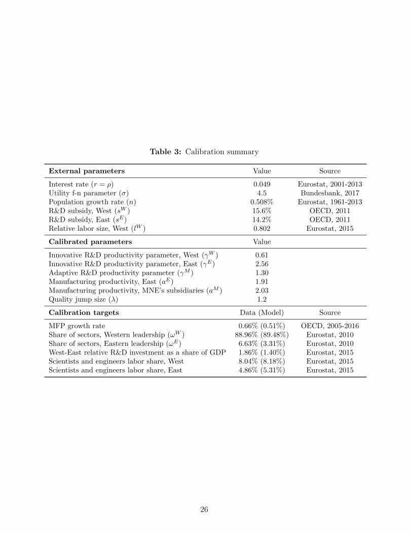
Table 3: Calibration summary

External parameters Value Source

Interest rate (r = ρ) 0.049 Eurostat, 2001-2013Utility f-n parameter (σ) 4.5 Bundesbank, 2017Population growth rate (n) 0.508% Eurostat, 1961-2013R&D subsidy, West (sW ) 15.6% OECD, 2011R&D subsidy, East (sE) 14.2% OECD, 2011Relative labor size, West (lW ) 0.802 Eurostat, 2015

Calibrated parameters Value

Innovative R&D productivity parameter, West (γW ) 0.61Innovative R&D productivity parameter, East (γE) 2.56Adaptive R&D productivity parameter (γM ) 1.30Manufacturing productivity, East (aE) 1.91Manufacturing productivity, MNE’s subsidiaries (aM ) 2.03Quality jump size (λ) 1.2

Calibration targets Data (Model) Source

MFP growth rate 0.66% (0.51%) OECD, 2005-2016Share of sectors, Western leadership (ωW ) 88.96% (89.48%) Eurostat, 2010Share of sectors, Eastern leadership (ωE) 6.63% (3.31%) Eurostat, 2010West-East relative R&D investment as a share of GDP 1.86% (1.40%) Eurostat, 2015Scientists and engineers labor share, West 8.04% (8.18%) Eurostat, 2015Scientists and engineers labor share, East 4.86% (5.31%) Eurostat, 2015

26

GDP and Foreign Direct Investment (FDI) within-EU27 and external.24 We proceed as follows:

first, we exclude the external (non-EU) FDI stock in the EU27 area from the regions’ and the

area’s total GDP. The share of EU15 GDP (excluding FDI from the EU12 to the EU15) in the

total EU27 GDP represents the target for the share of sectors with western leadership, ωW .

The share of EU12 GDP (excluding EU15 FDI in the EU12) in the total EU27 GDP is used

as a target for the share of sectors with East leadership, ωE. Finally, we use the EU15 FDI

stock in the EU12 as a share of the EU27 GDP to represent the share of sectors under the

control of Western subsidiary firms in the East, ωM . A more detailed description of this part of

the calibration strategy can be found in Appendix (B.1). The parameters’ values are obtained

by minimising the quadratic distance between the model steady state and the statistics listed

above. We summarize the calibration results in Table 3. Except for falling short of matching

the share of sectors with eastern leadership, our stylised model performs fairly well in fitting

the data targets.

4.2 Unilateral changes in R&D subsidies

We begin our analysis exploring the effects of R&D subsidies and their underlying mechanisms

in each region. More precisely, we keep the R&D subsidy of a region constant at the benchmark

value and describe the effects of changing the subsidy in the other region. The results are useful

in understanding the outcomes of the policy games that we analyse later.

Subsidising R&D in the West. In the first experiment, we keep the R&D subsidy of a

region constant at the benchmark value and describe the effects of changing the subsidy of

the other region. Figure 4 shows the effects of changing the western subsidy in an interval

of the benchmark value.25 An increase in the western subsidy stimulates the sectoral level of

innovation in the West, IW , as it reduces the cost of innovation. Higher western innovation

implies more creative destruction for eastern firms and therefore, successful innovators there

expect a lower duration of their leadership; as can be seen in the free entry condition (15). As

a consequence, the return to innovation in the East declines and with it the innovation rate

IE. Moreover, a higher western subsidy increases adaptive R&D investment and production

transfer to the East, IM . The free entry condition (16) suggests that the decision to transfer

technology and production abroad is pinned down by the difference in labor cost and in creative

destruction. For a given wage difference, a higher level of innovation in the West and a lower

24EU27 stands for the European Union of the year 2007, i.e before the latest addition of Croatia as itsmember in 2013. It consists of the two groups: EU15 (old members, the West) which includes Belgium, France,Germany, Italy, Luxembourg, the Netherlands, Denmark, Ireland, the U.K., Greece, Portugal, Spain, Austria,Finland and Sweden, and the EU12 (new members, the East) which includes Cyprus, Czech Republic, Estonia,Hungary, Latvia, Lithuania, Malta, Poland, Slovakia, Slovenia, Bulgaria and Romania.

25We choose an interval between a 5% and and 25% subsidy which roughly represent the minimum andmaximum government support due to tax incentives in Figure 3.

27

in the East implies that western firms face a lower risk of being leapfrogged by eastern firms

when moving their production abroad. Hence, a higher western subsidy increases the incentive

to transfer technology and production abroad.26

The changes in innovation described above affect the geographical distribution of market

leadership. The set of sectors with direct West leadership ωW decreases, while the set with

western multinational leadership ωM increases. Interestingly, although adaptive innovation is

performed by western firms in the East, and therefore does not benefit from western R&D

subsidies, it experiences a stronger growth following an increase in sW then western innovation:

the former rises by about 60% while the latter rises by 25% when sW rises from its benchmark of

15.6% to 25%. Thus, the general equilibrium effect of the subsidy through creative destruction is

stronger than the direct effect via the reduction of innovation costs, and higher western subsidies

lead to an expanded western leadership through multinational production. Notice also that the

increase in technology and production transfer triggers an increase in labor demand in the East

relative to the West, thereby leading to an increase in eastern relative wage.

Higher western subsidies trigger a higher global growth rate. This happens because the

subsidy increases innovation per sector in the West, IW , the region that innovates in all sectors

of the economy, and reduces innovation per sector in the East, where firms only innovate in a

subset of industries. As we can see in the growth equation (19), an increase IW raises growth,

while a reduction in IE and an increase share of production taking place in the East (ωE +ωM),

which implies an increase in 1− qW , reduces growth. Since, even at the maximum subsidy level

that we consider the West leads in more than 85% of sectors, the increase in western innovation

dominates and higher western subsidies propel higher global growth.

Welfare in the West increases with western R&D subsidies. In Figure 5, we decompose the

welfare effect into its different parts as in (31) and find a positive contribution of the growth

channel, while the expenditure channel is less straightforward. Equation (25) suggests that

besides the negative effect on consumption expenditures of the increased tax burden needed to

finance the R&D subsidy, the only other impact takes place through the value of the total assets

AW (equation 44). The value of western assets increases due to a rise in the share of sectors

with western leadership (ωW + ωM), caused by higher innovation and multinational transfer.

However, the tax burden which increases with the subsidy overturns this positive effect and

reduces the consumption component of the welfare. Next, western firms shifting production to

the East via FDI implies that the static component of aggregate prices declines, as labor cost

is lower in the East.27 Finally, the growth component is positive and strong, and along with

26Similarly to Dinopoulos and Segerstrom (2010), lower creative destruction in the less developed countryattracts more multinational production transfer. In their model though, creative destruction in the South isthe exogenous rate at which North technologies are copied there, while here it is the endogenous response ofeastern firms innovation to western subsidies. Hence, this effect of R&D on FDI cannot be obtained in modelswhere the less developed region does not innovate.

27Recall from (13) that P =[qW pW (1−σ) + qMpM(1−σ) + qEpE(1−σ)] 1

1−σ is the contribution of western quality

28

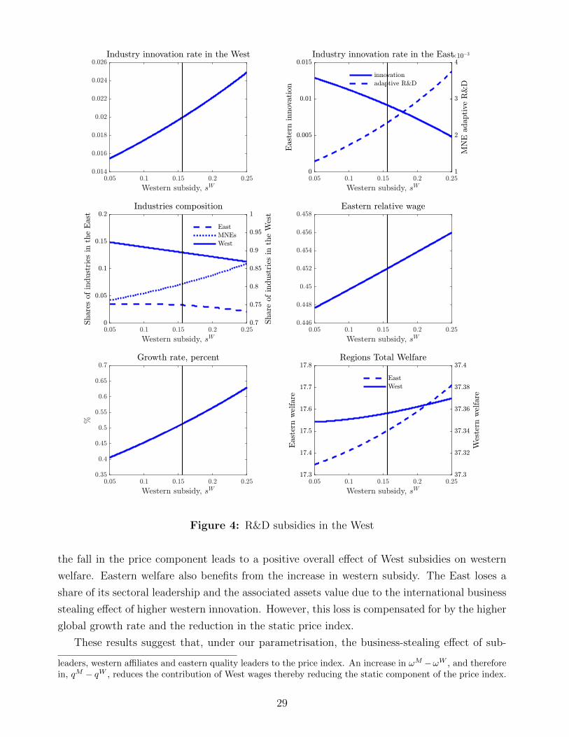
Figure 4: R&D subsidies in the West

the fall in the price component leads to a positive overall effect of West subsidies on western

welfare. Eastern welfare also benefits from the increase in western subsidy. The East loses a

share of its sectoral leadership and the associated assets value due to the international business

stealing effect of higher western innovation. However, this loss is compensated for by the higher

global growth rate and the reduction in the static price index.

These results suggest that, under our parametrisation, the business-stealing effect of sub-

leaders, western affiliates and eastern quality leaders to the price index. An increase in ωM −ωW , and thereforein, qM − qW , reduces the contribution of West wages thereby reducing the static component of the price index.

29

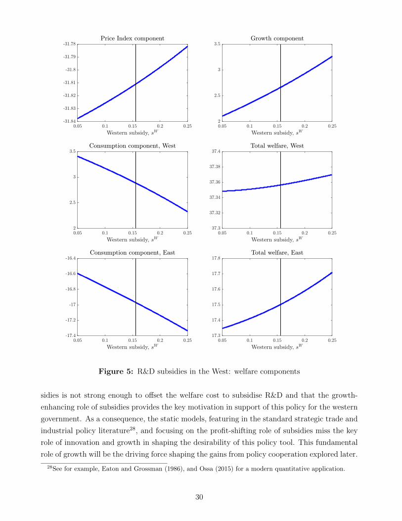
Figure 5: R&D subsidies in the West: welfare components

sidies is not strong enough to offset the welfare cost to subsidise R&D and that the growth-

enhancing role of subsidies provides the key motivation in support of this policy for the western

government. As a consequence, the static models, featuring in the standard strategic trade and

industrial policy literature28, and focusing on the profit-shifting role of subsidies miss the key

role of innovation and growth in shaping the desirability of this policy tool. This fundamental

role of growth will be the driving force shaping the gains from policy cooperation explored later.

28See for example, Eaton and Grossman (1986), and Ossa (2015) for a modern quantitative application.

30

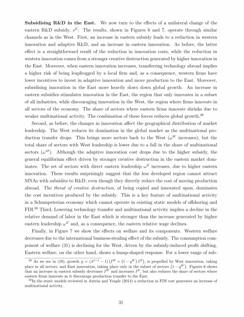
Subsidising R&D in the East. We now turn to the effects of a unilateral change of the

eastern R&D subsidy, sE. The results, shown in Figures 6 and 7, operate through similar

channels as in the West. First, an increase in eastern subsidy leads to a reduction in western

innovation and adaptive R&D, and an increase in eastern innovation. As before, the latter

effect is a straightforward result of the reduction in innovation costs, while the reduction in

western innovation comes from a stronger creative destruction generated by higher innovation in

the East. Moreover, when eastern innovation increases, transferring technology abroad implies

a higher risk of being leapfrogged by a local firm and, as a consequence, western firms have

lower incentives to invest in adaptive innovation and move production to the East. Moreover,

subsidising innovation in the East more heavily slows down global growth. An increase in

eastern subsidies stimulates innovation in the East, the region that only innovates in a subset

of all industries, while discouraging innovation in the West, the region where firms innovate in

all sectors of the economy. The share of sectors where eastern firms innovate shrinks due to

weaker multinational activity. The combination of these forces reduces global growth.29

Second, as before, the changes in innovation affect the geographical distribution of market

leadership. The West reduces its domination in the global market as the multinational pro-

duction transfer drops. This brings more sectors back to the West (ωW increases), but the

total share of sectors with West leadership is lower due to a fall in the share of multinational

sectors (ωM). Although the adaptive innovation cost drops due to the higher subsidy, the

general equilibrium effect driven by stronger creative destruction in the eastern market dom-

inates. The set of sectors with direct eastern leadership ωE increases, due to higher eastern

innovation. These results surprisingly suggest that the less developed region cannot attract

MNAs with subsidies to R&D, even though they directly reduce the cost of moving production

abroad. The threat of creative destruction, of being copied and innovated upon, dominates

the cost incentives produced by the subsidy. This is a key feature of multinational activity

in a Schumpeterian economy which cannot operate in existing static models of offshoring and

FDI.30 Third, Lowering technology transfer and multinational activity implies a decline in the

relative demand of labor in the East which is stronger than the increase generated by higher

eastern leadership ωE and, as a consequence, the eastern relative wage declines.

Finally, in Figure 7 we show the effects on welfare and its components. Western welfare

decreases due to the international business-stealing effect of the subsidy. The consumption com-

ponent of welfare (31) is declining for the West, driven by the subsidy-induced profit shifting.

Eastern welfare, on the other hand, shows a hump-shaped response. For a lower range of sub-

29 As we see in (19), growth g = (λσ−1 − 1)(IW +

(1− qW

)IE), is propelled by West innovation, taking

place in all sectors, and East innovation, taking place only in the subset of sectors(1− qW

). Figures 6 shows

that an increase in eastern subsidy decreases IW and increases IE , but also reduces the share of sectors whereeastern firms innovate as it discourage production transfer to the East.

30In the static models reviewed in Antras and Yeaple (2014) a reduction in FDI cost generates an increase ofmultinational activity.

31

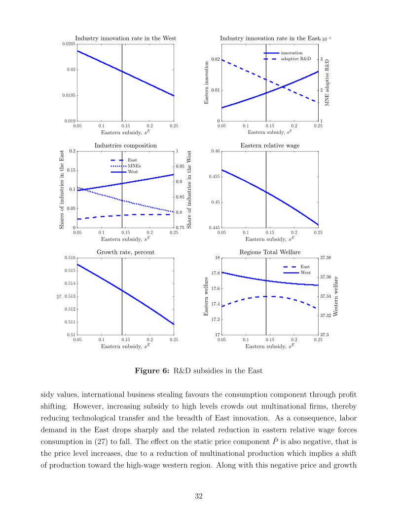
Figure 6: R&D subsidies in the East

sidy values, international business stealing favours the consumption component through profit

shifting. However, increasing subsidy to high levels crowds out multinational firms, thereby

reducing technological transfer and the breadth of East innovation. As a consequence, labor

demand in the East drops sharply and the related reduction in eastern relative wage forces

consumption in (27) to fall. The effect on the static price component P is also negative, that is

the price level increases, due to a reduction of multinational production which implies a shift

of production toward the high-wage western region. Along with this negative price and growth

32

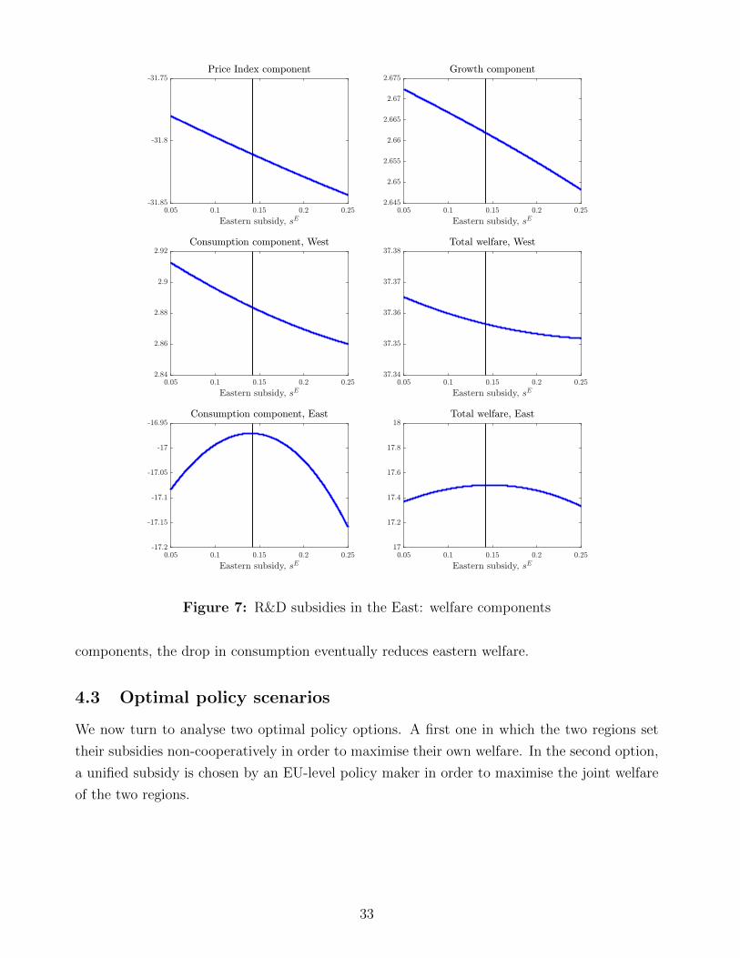
Figure 7: R&D subsidies in the East: welfare components

components, the drop in consumption eventually reduces eastern welfare.

4.3 Optimal policy scenarios

We now turn to analyse two optimal policy options. A first one in which the two regions set

their subsidies non-cooperatively in order to maximise their own welfare. In the second option,

a unified subsidy is chosen by an EU-level policy maker in order to maximise the joint welfare

of the two regions.

33

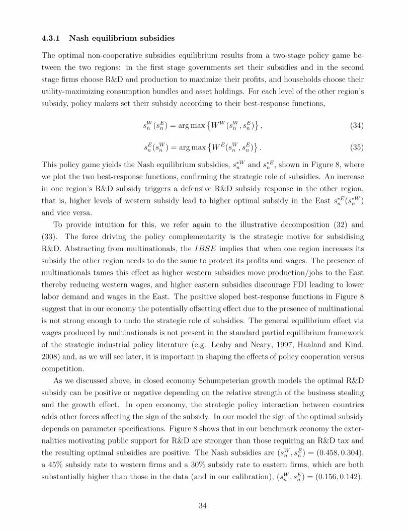
4.3.1 Nash equilibrium subsidies

The optimal non-cooperative subsidies equilibrium results from a two-stage policy game be-

tween the two regions: in the first stage governments set their subsidies and in the second

stage firms choose R&D and production to maximize their profits, and households choose their

utility-maximizing consumption bundles and asset holdings. For each level of the other region’s

subsidy, policy makers set their subsidy according to their best-response functions,

sWn (sEn ) = arg max{WW (sWn , s

En )}, (34)

sEn (sWn ) = arg max{WE(sWn , s

En )}. (35)

This policy game yields the Nash equilibrium subsidies, s∗Wn and s∗En , shown in Figure 8, where

we plot the two best-response functions, confirming the strategic role of subsidies. An increase

in one region’s R&D subsidy triggers a defensive R&D subsidy response in the other region,

that is, higher levels of western subsidy lead to higher optimal subsidy in the East s∗En (s∗Wn )

and vice versa.

To provide intuition for this, we refer again to the illustrative decomposition (32) and

(33). The force driving the policy complementarity is the strategic motive for subsidising

R&D. Abstracting from multinationals, the IBSE implies that when one region increases its

subsidy the other region needs to do the same to protect its profits and wages. The presence of

multinationals tames this effect as higher western subsidies move production/jobs to the East

thereby reducing western wages, and higher eastern subsidies discourage FDI leading to lower

labor demand and wages in the East. The positive sloped best-response functions in Figure 8

suggest that in our economy the potentially offsetting effect due to the presence of multinational

is not strong enough to undo the strategic role of subsidies. The general equilibrium effect via

wages produced by multinationals is not present in the standard partial equilibrium framework

of the strategic industrial policy literature (e.g. Leahy and Neary, 1997, Haaland and Kind,

2008) and, as we will see later, it is important in shaping the effects of policy cooperation versus

competition.

As we discussed above, in closed economy Schumpeterian growth models the optimal R&D

subsidy can be positive or negative depending on the relative strength of the business stealing

and the growth effect. In open economy, the strategic policy interaction between countries

adds other forces affecting the sign of the subsidy. In our model the sign of the optimal subsidy

depends on parameter specifications. Figure 8 shows that in our benchmark economy the exter-

nalities motivating public support for R&D are stronger than those requiring an R&D tax and

the resulting optimal subsidies are positive. The Nash subsidies are (sWn , sEn ) = (0.458, 0.304),

a 45% subsidy rate to western firms and a 30% subsidy rate to eastern firms, which are both

substantially higher than those in the data (and in our calibration), (sWn , sEn ) = (0.156, 0.142).

34

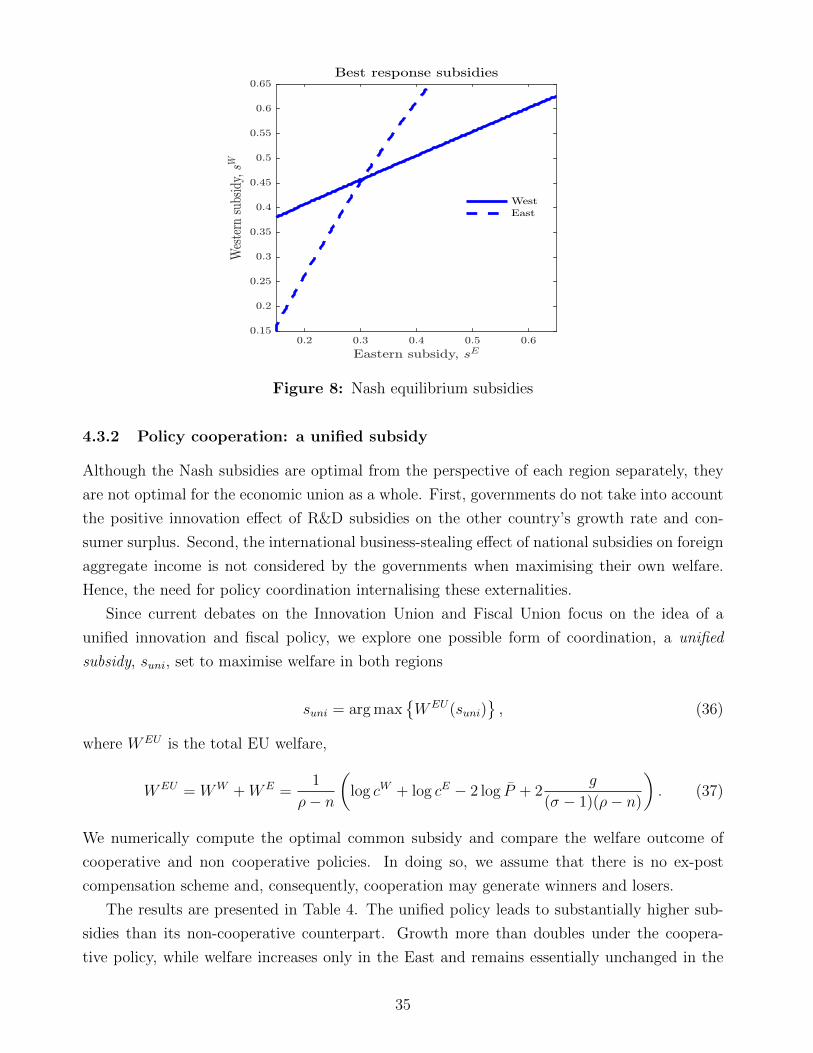
Figure 8: Nash equilibrium subsidies

4.3.2 Policy cooperation: a unified subsidy

Although the Nash subsidies are optimal from the perspective of each region separately, they

are not optimal for the economic union as a whole. First, governments do not take into account

the positive innovation effect of R&D subsidies on the other country’s growth rate and con-

sumer surplus. Second, the international business-stealing effect of national subsidies on foreign

aggregate income is not considered by the governments when maximising their own welfare.

Hence, the need for policy coordination internalising these externalities.

Since current debates on the Innovation Union and Fiscal Union focus on the idea of a

unified innovation and fiscal policy, we explore one possible form of coordination, a unified

subsidy, suni, set to maximise welfare in both regions

suni = arg max{WEU(suni)

}, (36)

where WEU is the total EU welfare,

WEU = WW +WE =1

ρ− n

(log cW + log cE − 2 log P + 2

g

(σ − 1)(ρ− n)

). (37)

We numerically compute the optimal common subsidy and compare the welfare outcome of

cooperative and non cooperative policies. In doing so, we assume that there is no ex-post

compensation scheme and, consequently, cooperation may generate winners and losers.

The results are presented in Table 4. The unified policy leads to substantially higher sub-

sidies than its non-cooperative counterpart. Growth more than doubles under the coopera-

tive policy, while welfare increases only in the East and remains essentially unchanged in the

35

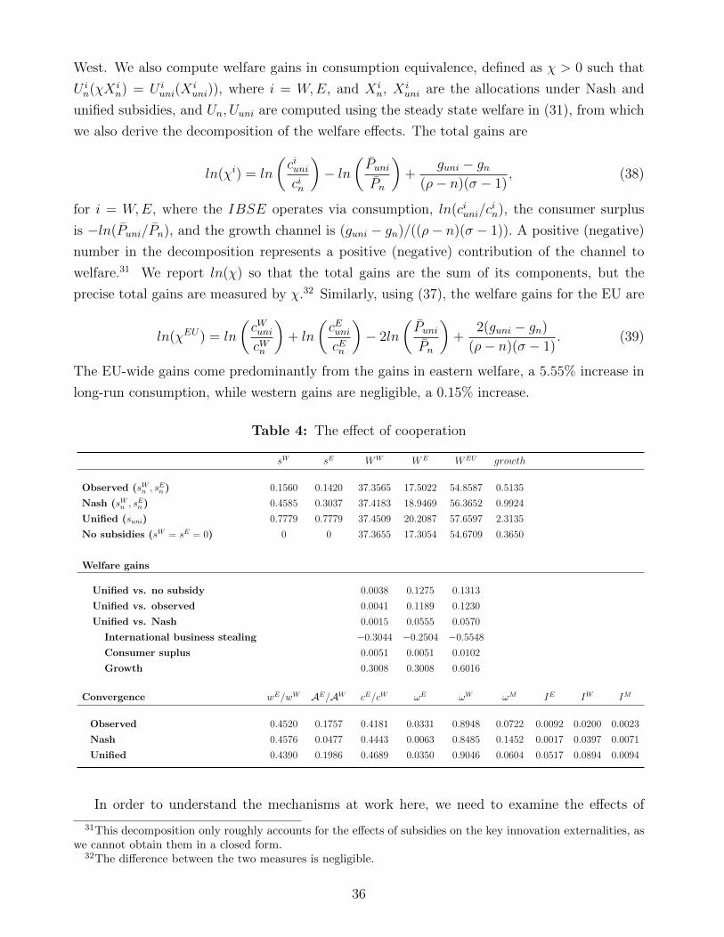
West. We also compute welfare gains in consumption equivalence, defined as χ > 0 such that

U in(χX i

n) = U iuni(X

iuni)), where i = W,E, and X i

n, X iuni are the allocations under Nash and

unified subsidies, and Un, Uuni are computed using the steady state welfare in (31), from which

we also derive the decomposition of the welfare effects. The total gains are

ln(χi) = ln

(ciunicin

)− ln

(PuniPn

)+

guni − gn(ρ− n)(σ − 1)

, (38)

for i = W,E, where the IBSE operates via consumption, ln(ciuni/cin), the consumer surplus

is −ln(Puni/Pn), and the growth channel is (guni − gn)/((ρ− n)(σ − 1)). A positive (negative)

number in the decomposition represents a positive (negative) contribution of the channel to

welfare.31 We report ln(χ) so that the total gains are the sum of its components, but the

precise total gains are measured by χ.32 Similarly, using (37), the welfare gains for the EU are

ln(χEU) = ln

(cWunicWn

)+ ln

(cEunicEn

)− 2ln

(PuniPn

)+

2(guni − gn)

(ρ− n)(σ − 1). (39)

The EU-wide gains come predominantly from the gains in eastern welfare, a 5.55% increase in

long-run consumption, while western gains are negligible, a 0.15% increase.

Table 4: The effect of cooperation

sW sE WW WE WEU growth

Observed (sWn , sEn ) 0.1560 0.1420 37.3565 17.5022 54.8587 0.5135

Nash (sWn , sEn ) 0.4585 0.3037 37.4183 18.9469 56.3652 0.9924

Unified (suni) 0.7779 0.7779 37.4509 20.2087 57.6597 2.3135

No subsidies (sW = sE = 0) 0 0 37.3655 17.3054 54.6709 0.3650

Welfare gains

Unified vs. no subsidy 0.0038 0.1275 0.1313

Unified vs. observed 0.0041 0.1189 0.1230

Unified vs. Nash 0.0015 0.0555 0.0570

International business stealing −0.3044 −0.2504 −0.5548

Consumer suplus 0.0051 0.0051 0.0102

Growth 0.3008 0.3008 0.6016

Convergence wE/wW AE/AW cE/cW ωE ωW ωM IE IW IM

Observed 0.4520 0.1757 0.4181 0.0331 0.8948 0.0722 0.0092 0.0200 0.0023

Nash 0.4576 0.0477 0.4443 0.0063 0.8485 0.1452 0.0017 0.0397 0.0071

Unified 0.4390 0.1986 0.4689 0.0350 0.9046 0.0604 0.0517 0.0894 0.0094

In order to understand the mechanisms at work here, we need to examine the effects of

31This decomposition only roughly accounts for the effects of subsidies on the key innovation externalities, aswe cannot obtain them in a closed form.

32The difference between the two measures is negligible.

36

subsidies on the objective function WEU . Below we present an illustrative decomposition based

on (39). Starting with the effects of the West subsidy we have,

∂WEU

∂sW=

∂cW

∂sW︸︷︷︸BSE

(−)

+∂cW

∂sW︸︷︷︸IBSE

(+/−)

+∂cE

∂sW︸︷︷︸IBSE

(+/−)

+ 2∂P

∂sW︸ ︷︷ ︸CSE

(+)

+ 2∂g

∂sW︸ ︷︷ ︸GRE

(+)

. (40)

Comparing (40) with (32) suggests that the unified subsidy internalises the business stealing,

the consumer surplus effect and the growth effect of western subsidies on the other region.

Internalising the strategic motive for subsidy, the IBSE externality should lead to a unified

subsidy lower than the Nash in both regions. The results in Table 4 show that the opposite

happens, the unified subsidy is substantially larger than the Nash subsidies. The driving

force of this result is that policy cooperation also internalises the consumer surplus and the

growth effect of one country’s subsidies on the other country’s welfare. Under our benchmark

parametrisation, the internalisation of the positive growth effect and of the consumer surplus

effect dominate, thereby leading to a higher unified R&D subsidy than the Nash subsidies.

Hence, the key reason for setting a common subsidy is not the correction of the strategic

motive but the strong consumer surplus and the growth effect it produces.

This result echoes those in Leahy and Neary (1997 and 2009) and Haaland and Kind (2008),

who show, in simpler frameworks, that when innovation spillovers are high, the consumer

surplus effect is strong and subsidies under cooperation are higher than under Nash. In our

dynamic setting knowledge spillovers impact welfare via an additional, intertemporal channel,

the growth effect which proves to be quantitatively powerful and the key driver of the result,

as we show below.

The illustrative decomposition of the effects of eastern subsidy based on (39) is,

∂WEU

∂sE=

∂cE

∂sE︸︷︷︸BSE

(−)

+∂cE

∂sE︸︷︷︸IBSE

(+)

+∂cW

∂sE︸︷︷︸IBSE

(−)

+ 2∂P

∂sE︸ ︷︷ ︸GRE

(+)

+ 2∂g

∂sE︸ ︷︷ ︸CSE

(+/−)

. (41)

For the East, internalising the IBES also implies a smaller unified subsidy compared to Nash,

but, differently from the West, eastern R&D subsidies can reduce global growth as they dis-

courage FDI thereby reducing the scope of eastern innovation (the share of sectors where the

eastern firms innovate). The results show that the unified subsidy is substantially higher than

the Nash subsidy in the East as well. This suggests that, similarly to what we saw for the

West, the internalisation of the consumer surplus effect and of the growth effect drive of the

gains from policy cooperation.

37

In Table 4, we present a decomposition of the welfare gains from the unified subsidy com-

pared to the Nash based on (39) which heuristically tracks the internalisation of the three

externalities shown in (40) and (41). The international business stealing component is neg-

ative. This suggests that the higher unified subsidy relative to Nash aggravates rather than

correcting the international business stealing externality. The welfare gains from cooperation

attributable to the consumer surplus effect are small, about half of a percentage point. While

the gains brought about by the internalisation of the growth effect are large. This suggests that

the internalisation of the consumer surplus effect of innovation (and production) subsidies, typ-

ical of the static strategic industrial policy models (e.g Eaton and Grossman, 1986, and Leahy

and Neary, 1997), is not sufficient to generate large welfare gains from cooperation. The key

externality driving the gains form cooperation is the growth effect, or intertemporal knowledge

spillover (Aghion and Howitt, 1992), which cannot be obtained in static models.

The results are similar when we compare the unified subsidy with a no policy intervention

scenario (zero subsidies) and with the observed subsidies. The gains from cooperation in these

scenarios for the EU as a whole are substantially larger compared to those in the Nash sce-

nario: long-run consumption is 13% higher compared to no policy intervention, and 12% higher

compared to the observed subsidies. Most of these gains are again concentrated in the East.33

Unequal gains. Why are the gains form cooperation unequally distributed? There are essen-

tially three reasons to cooperate: internalising the consumer surplus effect, the growth effect and

the IBSE. Since trade is free, internalising the first two externalities benefits both countries

equally. Internalising the business stealing effect, instead, has unequal welfare implications.

Since the unified subsidy is higher than the Nash subsidies, policy cooperation produces more

IBSE than the uncooperative scenario and the associated welfare losses are higher for the West

(−0.3)) than for the East (−0.25). This occurs because moving from the Nash to the unified

scenario produces a larger subsidy increase for the latter. This implies that the East ends

up stealing business from the West, thereby reducing its national income and consumption.

Another, perhaps more intuitive, way to understand this result is noticing that in the Nash

scenario the West leads in 99% of the sectors in the economy, either via direct leadership or

via multinationals, as can be seen in Table 4. Hence, the incentives to cooperate to reign in

East business stealing are then quite low. When the innovation asymmetries between the two

regions are smaller, as in the observed subsidies case, the incentives to cooperate for the West

are indeed larger.

Convergence. One of the key targets of the Innovation Union and of the comprehensive

Europe 2020 strategy, the EU’s agenda for growth and jobs for the current decade, is regional

33We only report the total gains, the decomposition produces the same results as in the Nash case, with thegrowth channel dominating, and are available upon request.

38

cohesion, which mandates that the EU policies should promote convergence across European

regions in innovation and growth performance (European Commission, 2015). We have then

analysed the impact of a unified innovation subsidy on convergence of income and innovation

performance. Table 4 shows relative income and innovation performance of the two regions

under the observed subsidies, the Nash and the unified subsidy.

The unified subsidy promotes income convergence across regions driven by convergence in

asset ownership, AE/AW , while it worsens the East-West gap in relative wages. Although the

relative eastern wage declines, the increase in the share of firms owned by eastern households

generates an increase in the income from assets stronger than the decline in relative wages,

thereby triggering convergence in consumption. Uniform subsidies imply an increase in subsidy

compared to Nash for both the East and the West, but more for the East. So we can understand

the convergence result simply thinking about an increase in the eastern subsidy while leaving

the western subsidy constant. A higher eastern subsidy increases the share of sectors led by

eastern firms ωE, thereby increasing the share of eastern assets. On the other hand the share

of sectors led by western multinationals shrinks, due to increasing creative destruction, and

this reduces FDI which, in turn, reduces the relative labor demand and wage in the East. The

convergence in market leadership and therefore in asset ownership is due to the convergence in

innovation, which can be observed in the last three columns of Table 4. Under Nash, innovation

by eastern firms accounts for about 3.5% of total innovation (IE/(IE + IW + IM)) and about

34% under unified subsidy. The convergence in income level and consumption are quite small

and, as we discussed above, most of the welfare gains for the East of adopting a unified subsidy

come from the growth effect and a reduction in the quality-adjusted prices, which increasing

households’ purchasing power.

5 Robustness and further analysis

Next, we first conduct robustness analysis with respect to some key parameters of our economy

and then explore the implications of unbundling the FDI and the R&D subsidy and of assuming

that FDI is financed by Western saving, a different asset ownership structure.

5.1 Robustness

Let us first consider an increase in the efficiency of MNE’s production transfer as a measure of

the regions’ integration. The efficiency of production transfer from the West to the East may

depend on many features of the real economy. It could be, for example, shaped by the level of

human capital in the East, by product standards and non-tariff barriers, such as regulations on

technology adoption. In our simple economy, it is captured in a simple way by the productivity

parameter of the adaptive R&D, γM .

39

In Table C.1 in the Appendix, we analyse how changes in the efficiency/cost of production

transfer affect the Nash and unified subsidies regimes. The Nash subsidies declines with the

efficiency of production transfer. As seen above, multinationals tame the strategic motive for

subsidy: with more FDI the regions are more integrated, the rewards for a subsidy war are

lower and, consequently, the optimal Nash subsidies are lower. The unified subsidy, instead,

increases when FDI is more efficient. On the one hand, since the strategic motive for subsidy

is weaker with more efficient FDI, the benefits from internalising the international business

stealing effect are lower and so should the unified subsidy. On the other hand, if internalising

the consumer surplus and growth effect becomes more important, the unified subsidy could

be higher. The innovation technology (8) suggests that an increase in FDI, by increasing

the breadth of innovation, raises the average quality in sectors where eastern firms innovate

(QE+M) thereby increasing the aggregate knowledge spillovers these firms are exposed to and

therefore their innovation efficiency. Stronger knowledge spillovers imply a stronger market

failure in innovation and a stronger incentive for the EU policy maker to correct it. The

larger gains from subsidy cooperation compared to competition come then from a larger role

for consumer surplus and growth while the business stealing externality plays a weaker role

compared to benchmark, as the strategic motive for subsidies is weaker with more FDI. As in

the benchmark case, the East reaps most of the gains from cooperation, while the gains for the

West are negligible.

In Table C.2, we explore robustness with respect to parameter σ, which regulates the

markup. Unfortunately, we can only check the robustness to small changes, as the equilibrium

is very sensitive around this parameter. Although changes are quite local, they do provide

some insight. A lower markup (higher σ), reduces the importance of the international business

stealing effect, as the strategic motive to shift profits across borders is driven by the size of

these rents. With smaller profits, policy cooperation does not need to make a strong effort to

internalise the IBSE which implies that the unified subsidy rises, as the growth channel be-

comes an ever stronger driver. However, in the absence of a large inefficiency operating through

the markup and IBSE cooperation generates smaller EU gains.

5.2 Extensions

Gains from cooperation: FDI vs. innovation policy. In our benchmark model, although

FDI does not directly contribute to innovation and growth, it benefits from the same subsidy

as innovative R&D. In this extension, instead, the economy features an innovation policy,

the R&D subsidy, and separate FDI subsidy, which can be seen as a more standard trade

policy, as it affect the cost of multinational activity with no direct implications for innovation.

With a few exceptions (e.g. Akcigit et al., 2018) innovation and trade policies are typically

analysed separately, in different models. Our framework allows a joint analysis and permits a

40

decomposition of the their specific contribution to the welfare gains from international policy

cooperation.

In Table C.3 we report a new Nash scenario where the West and the East maximise their

own welfare by setting the R&D subsidies (sWn , sEn ) non-cooperatively, and the East also sets

the FDI subsidy (sMn ) to maximise its own welfare. The optimal R&D subsidy for the East

is higher (0.35) than in the benchmark case (0.30). In the benchmark model a higher East

R&D subsidy, on the one hand, reduces the cost of FDI but, on the other hand, increases

innovation and creative destruction in the East thereby discouraging FDI. The former effect

strengthens the strategic motive for subsidies while the latter weakens it. In the new scenario,

instead, the former effect is zero by construction, as the R&D subsidy does not directly affect

the cost of FDI, thus we would expect a lower eastern Nash R&D subsidy. However, the

East finds it optimal to fully subsidise FDI (sM = 1). The optimal FDI subsidy reaches the

highest possible level because now it does not generate the negative effect on FDI via creative

destruction, as it is unbundled from the R&D subsidy and does not directly affect eastern firms’

innovation. As seen above, more FDI expands the set of sectors where eastern firms innovate

(QE+M) thereby increasing the aggregate knowledge spillovers in (8) for these firms. Due to

these higher spillovers the marginal effect of the East R&D subsidy on eastern welfare is larger

and thus the Nash R&D subsidy rises.

Next we compute a new cooperative policy regime characterised by the unified R&D subsidy

(suni) and the FDI subsidy (sMuni) set separately to maximise EU welfare. As we discussed above,

when RD and FDI subsidies are separated the internalisation of the IBSE is more important,

because the strategic motive for subsidy is stronger, but the growth effect is more powerful as

well, as the knowledge spillovers generated by specific subsidies to FDI are stronger. This latter

effect prevails and the optimal unified R&D subsidy is slightly higher than in the benchmark

scenario of Table 4. Both the growth and welfare gains produced by policy cooperation com-

pared to Nash are substantially larger than in the benchmark case. Now cooperation attains a

8.1% increase in long-run consumption, three percentage points larger than in the benchmark

scenario. Once again most of these gains are accounted for by internalising the growth effect.

To facilitate comparisons between these two scenarios we have summarised the welfare gains

result in column (1) and (2) of Table 5. These larger gains are obtained because now the policy

tools used can target more directly the two types of externalities: the R&D subsidy tackles

the innovation externalities and the FDI subsidy tackles the externalities related to technol-

ogy/production transfer. The complementarity between FDI and R&D subsidies produces the

larger gains from trade: more FDI leads to stronger international knowledge spillovers which,

in turn, strengthen the growth effect of innovation subsidies.

We now turn to the decomposition of the gains from cooperation in FDI and innovation

policy. In Table 5, we quantify the gains from optimal innovation and those from optimal FDI

41

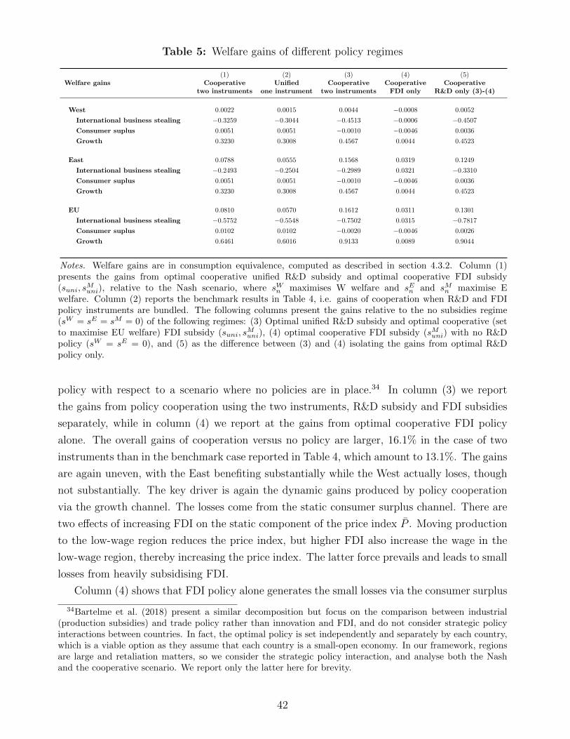
Table 5: Welfare gains of different policy regimes

(1) (2) (3) (4) (5)Welfare gains Cooperative Unified Cooperative Cooperative Cooperative

two instruments one instrument two instruments FDI only R&D only (3)-(4)

West 0.0022 0.0015 0.0044 −0.0008 0.0052

International business stealing −0.3259 −0.3044 −0.4513 −0.0006 −0.4507

Consumer suplus 0.0051 0.0051 −0.0010 −0.0046 0.0036

Growth 0.3230 0.3008 0.4567 0.0044 0.4523

East 0.0788 0.0555 0.1568 0.0319 0.1249

International business stealing −0.2493 −0.2504 −0.2989 0.0321 −0.3310

Consumer suplus 0.0051 0.0051 −0.0010 −0.0046 0.0036

Growth 0.3230 0.3008 0.4567 0.0044 0.4523

EU 0.0810 0.0570 0.1612 0.0311 0.1301

International business stealing −0.5752 −0.5548 −0.7502 0.0315 −0.7817

Consumer suplus 0.0102 0.0102 −0.0020 −0.0046 0.0026

Growth 0.6461 0.6016 0.9133 0.0089 0.9044

Notes. Welfare gains are in consumption equivalence, computed as described in section 4.3.2. Column (1)presents the gains from optimal cooperative unified R&D subsidy and optimal cooperative FDI subsidy(suni, s

Muni), relative to the Nash scenario, where sWn maximises W welfare and sEn and sMn maximise E

welfare. Column (2) reports the benchmark results in Table 4, i.e. gains of cooperation when R&D and FDIpolicy instruments are bundled. The following columns present the gains relative to the no subsidies regime(sW = sE = sM = 0) of the following regimes: (3) Optimal unified R&D subsidy and optimal cooperative (setto maximise EU welfare) FDI subsidy (suni, s

Muni), (4) optimal cooperative FDI subsidy (sMuni) with no R&D

policy (sW = sE = 0), and (5) as the difference between (3) and (4) isolating the gains from optimal R&Dpolicy only.

policy with respect to a scenario where no policies are in place.34 In column (3) we report

the gains from policy cooperation using the two instruments, R&D subsidy and FDI subsidies

separately, while in column (4) we report at the gains from optimal cooperative FDI policy

alone. The overall gains of cooperation versus no policy are larger, 16.1% in the case of two

instruments than in the benchmark case reported in Table 4, which amount to 13.1%. The gains

are again uneven, with the East benefiting substantially while the West actually loses, though

not substantially. The key driver is again the dynamic gains produced by policy cooperation

via the growth channel. The losses come from the static consumer surplus channel. There are

two effects of increasing FDI on the static component of the price index P . Moving production

to the low-wage region reduces the price index, but higher FDI also increase the wage in the

low-wage region, thereby increasing the price index. The latter force prevails and leads to small

losses from heavily subsidising FDI.

Column (4) shows that FDI policy alone generates the small losses via the consumer surplus

34Bartelme et al. (2018) present a similar decomposition but focus on the comparison between industrial(production subsidies) and trade policy rather than innovation and FDI, and do not consider strategic policyinteractions between countries. In fact, the optimal policy is set independently and separately by each country,which is a viable option as they assume that each country is a small-open economy. In our framework, regionsare large and retaliation matters, so we consider the strategic policy interaction, and analyse both the Nashand the cooperative scenario. We report only the latter here for brevity.

42

channel just discussed. Moreover, although growth still contributes positively to the gains from

setting the FDI subsidy cooperatively, it is not the main driver anymore. This is straightforward

as FDI does not contribute directly to innovation and growth. The gains now operate mostly

via increasing nominal income in the East, the IBSE. An increase in FDI increases the wage in

the East but, at the same time, reduces the value of the assets owned by eastern households,

as the difference between vM and vW in (45) goes to zero when the FDI subsidy is one, which

is the case under cooperation, as shown in Table C.3 . The wage effect dominates and eastern

income increases.

Column (5) reports the gains attributable to cooperative R&D policy only. The gains from

innovation policy alone are again concentrated in the East (12.49%) and are remarkably similar

to those obtained in the benchmark case with bundled subsidy in Table 4 (12.45%). The gains

for the EU in the two cases are identical. This suggests that tying the FDI policy to the

innovation policy does not generate any additional gains. While comparing (4) and (5) we

can see that a separate FDI subsidy produces extra gains equivalent to about 3% higher long-

run consumption. As in the benchmark case, the strong innovation policy under cooperation

is always harmful through the IBSE channel and always beneficial via the growth channel,

which is now stronger. The source of the larger gains is the complementarity between FDI

and innovation subsidies operating via the effect of the latter on the width and strength of

knowledge spillovers.

Alternative asset specification. Next, we explore an alternative assets specification where

the adaptive R&D, or FDI cost, which allows the West to transfer production to the East

is financed by western savings. In this case, western consumers appropriate the extra profit

obtained through cheaper MNE’s production. The key departure is that the asset values (44)

and (45) now become35

AW =

∫ωW

vW (ω)

LW (t)dω +

∫ωM

vM(ω)

LW (t)dω, AE =

∫ωE

vE

LE(t)(ω)dω.

The West can appropriate the full value of transferring production and this increases the strate-

gic motive to subsidise R&D in the West and move production abroad. In Table (C.4), we report

the Nash, the unified subsidy and their welfare and growth implications under this alternative

asset allocation. Higher rents from production transfer incentivise FDI and promote stronger

western innovation which in turn triggers higher business stealing effects and a stronger policy

response in the form of a significantly higher Nash subsidies. For the East, now FDI is less

effective in taming the strategic motive for subsidy, as it does not get the extra profit of western

multinationals. Hence, a higher strategic motive leads to a higher Nash subsidy for the East

35The derivation of the new asset values and the effect of unilateral subsidy change are shown in the AppendixC.1.

43

as well. In such a scenario with high Nash subsidies, cooperation is less driven by the growth

channel relative to the benchmark scenario, while the IBSE internalisation is more important

and generates larger gains (or smaller losses) compared to the benchmark. Overall, welfare

gains are still substantial but smaller than in our benchmark scenario.

In the Appendix, we also present the results of the unbundled FDI and R&D policies exercise

in Table (C.5) and (C.6) and show that the key findings are essentially confirmed under this

alternative asset allocation.

6 Conclusion

In this paper we have documented large asymmetries in innovation performance and policy

between old and new members of the European Union. We have also presented robust firm-level

evidence of western FDI spillovers on eastern firms’ innovation. Motivated by these facts and

by EU plans for further integration of innovation policy we have built a two-region endogenous

growth model to analyse the cost and benefits of innovation policy cooperation in an economic

union. The two regions feature firms competing in innovation for market leadership and are

integrated via free trade and costly technology transfer via FDI.

We have shown that cooperation in the form of a unified subsidy at the Union level gener-

ates large welfare gains compared to the non-cooperative Nash subsidy scenario. Most of these

gains come from the internalisation of the effect of subsidies on the growth rate of the econ-

omy. These dynamic gains are substantially larger than the static gains from internalising the

strategic motive for subsidies according to which countries compete to steal wages and profits

from each other. The presence of technology transfer and multinational production tames the

strategic motive for subsidies and increases the gains from cooperation. We have also shown

that unbundling the innovation policy, the RD subsidy, from the FDI subsidy, a more standard

trade policy, leads to larger gains from policy cooperation. This policy complementarity arises

from international knowledge spillovers brought about by Western FDI. By allowing eastern

firms to start innovating in a larger number of industries and by increasing their innovation

efficiency, FDI increase the marginal effect of R&D subsidies on innovation and growth.

For simplicity, we abstract from a third non-EU country (rest of the World) and focus on

two regions as a first step towards analysing the theoretical mechanisms driving the incentives

to cooperate in innovation policy within an economic union. Introducing a third country would

be an important generalisation, but its inclusion would complicate the analysis substantially

for the current purpose. We leave this challenging generalisation to future research.

44

References

Acemoglu, Daron and Ufuk Akcigit, “Intellectual Property Rights Policy, CompetitionAnd Innovation,” Journal of the European Economic Association, 2012, 10 (1), 1–42.

, Gino Gancia, and Fabrizio Zilibotti, “Offshoring and Directed Technical Change,”American Economic Journal: Macroeconomics, 2015, 7 (3), 84–122.

, Ufuk Akcigit, Harun Alp, Nicholas Bloom, and William R. Kerr, “Innovation,Reallocation and Growth,” American Economic Review, 2018, 108 (11), 3450–3491.

Aghion, Philippe and Peter Howitt, “A Model of Growth Through Creative Destruction,”Econometrica, 1992, 10 (1), 1–42.

Akcigit, Ufuk, Douglas Hanley, and Stefanie Stantcheva, “Optimal Taxation and R&DPolicies,” 2016. National Bureau of Economic Research Working Paper 22908.

, Sina T. Ates, and Giammario Impullitti, “Innovation and Trade Policy in a GlobalizedWorld,” 2018. NBER Working Papers 24543.

Antras, Pol and Stephen R. Yeaple, Multinational Firms and the Structure of InternationalTrade, Vol. 4 of Handbook of International Economics,

Arkolakis, Costas, Natalia Ramondo, Andres Rodrıguez-Clare, and StephenYeaple, “Innovation and Production in the Global Economy,” American Economic Review,2018, 108 (8), 2128–2173.

Audretsch, David B. and Maryann P. Feldman, “Knowledge Spillovers and the Geogra-phy of Innovation,” in J. Vernon Henderson and Jacque Thisse, eds., Handbook of Urban andRegional Economics: Cities and Geography, Vol. 4, Amsterdam: North Holland Publishing,2003, pp. 2713–2739.

Bartelme, Dominick, Arnaud Costinot, Dave Donaldson, and Andres Rodriguez-Clare, “Economies of Scale and Industrial Policy: A View from Trade,” 2018. mimeo.

Berger, Helge, Giovanni Dell’Ariccia, and Maurice Obstfeld, “Revisiting the EconomicCase for Fiscal Union in the Euro Area,” IMF Departmental Papers 18/03 2018.

Blomstrom, Magnus and Ari Kokko, “The Impact of Foreign Investment on Host Coun-tries: A Review of the Empirical Evidence,” World Bank Policy Research Working Paper,1997, (1745).

Campolmi, Alessia, Harald Fadinger, and Chiara Forlati, “Trade and Domestic Policiesin Models with Monopolistic Competition,” 2018. CEPR Discussion Papers 13219.

Dinopoulos, Elias and Paul Segerstrom, “Intellectual property rights, multinational firmsand economic growth,” Journal of Development Economics, 2010, 92 (1), 13–27.

and Peter Thompson, “Schumpeterian Growth without Scale Effects,” Journal of Eco-nomic Growth, 1998, 3 (4), 313–335.

45

d’Andria, Diego, Dimitris Pontikakis, and Agnieszka Skonieczna, “Towards a Euro-pean R&D Incentive? An assessment of R&D Provisions under a Common Corporate TaxBase,” 2017. Directorate General Taxation and Customs Union, European Commission.

Eaton, Jonathan and Gene M. Grossman, “Optimal Trade and Industrial Policy underOligopoly,” Quarterly Journal of Economics, 1986, 101 (2), 383–406.

European Commission, “State of the Union,” 2015. Directorate-General for Research andInnovation.

Felbermayr, Gabriel, Benjamin Jung, and Mario Larch, “Optimal tariffs, retaliation,and the welfare loss from tariff wars in the Melitz model,” Journal of International Eco-nomics, 2013, 89 (1), 13–25.

Gorg, Holger and David Greenaway, “Much Ado about Nothing? Do Domestic FirmsReally Benefit from Foreign Direct Investment?,” World Bank Research Observer, 2004, 19(2), 171–198.

Gorodnichenko, Yuriy, Jan Svejnar, and Katherine Terrell, “Globalization and Inno-vation in Emerging Markets,” American Economic Journal: Macroeconomics, 2010, 2 (2),194–226.

, , and , “Does Foreign Entry Spur Innovation?,” CEPR working paper, N10757, 2015.

Grossman, Gene M. and Edwin L.-C. Lai, “International Protection of Intellectual Prop-erty,” American Economic Review, 2004, 94 (5), 1635–1653.

and Elhanan Helpman, Innovation and Growth In the Global Economy, MIT press, 1991.

and , “Quality Ladders in the Theory of Growth,” Review of Economic Studies, 1991, 58(1), 43–61.

Haaland, Jan I. and Hans Jarle Kind, “R&D Policies, Trade and Process Innovation,”Journal of International Economics, 2008, 74 (1), 170–187.

Howitt, Peter, “Steady Endogenous Growth with Population and R & D Inputs Growing,”Journal of Political Economy, 1999, 107 (4), 715–730.

Impullitti, Giammario, “International Competition and US R&D Subsidies: A QuantitativeWelfare Analysis,” International Economic Review, 2010, 51 (4), 1127–1158.

and Omar Licandro, “Trade, Firm Selection, and Innovation: The Competition Channel,”Economic Journal, 2018, 128 (608), 189–229.

Javorcik, Beata Smarzynska, “Does Foreign Direct Investment Increase the Productivity ofDomestic Firms? In Search of Spillovers Through Backward Linkages,” American EconomicReview, june 2004, 94 (3), 605–627.

Jones, Charles, “RD-Based Models of Economic Growth,” Journal of Political Economy,1995, 103 (4), 759–784.

Kondo, Hiroki, “International R&D subsidy competition, industrial agglomeration andgrowth,” Journal of International Economics, 2013, 89 (1), 233–251.

46

Leahy, Dermot and J. Peter Neary, “Public Policy towards R&D in Oligopolistic Indus-tries,” American Economic Review, 1997, 87 (4), 642–662.

and , “Multilateral subsidy game,” Economic Theory, 2009, 41 (1), 41–66.

Maggi, Giovanni, “Strategic Trade Policies with Endogenous Mode of Competition,” Amer-ican Economic Review, 1996, 86 (1), 237–258.

Ossa, Ralph, “A ”New Trade” Theory of GATT/WTO Negotiations,” Journal of PoliticalEconomy, 2011, 119 (1), 122–152.

, “Trade Wars and Trade Talks with Data,” American Economic Review, 2014, 104 (12),4104–4146.

, “A Quantitative Analysis of Subsidy Competition in the US,” 2015. National Bureau ofEconomic Research Working Paper 20975.

Perla, Jesse, Christopher Tonetti, and Michael E. Waugh, “Equilibrium TechnologyDiffusion, Trade, and Growth,” 2015. National Bureau of Economic Research Working Paper20881.

Sampson, Thomas, “Dynamic Selection: An Idea Flows Theory of Entry, Trade, andGrowth,” Quarterly Journal of Economics, 2016, 131 (1), 315–380.

Segerstrom, Paul S., “Endogenous Growth without Scale Effects,” American Economic Re-view, 1998, 88, 1290–1310.

and Amanda Jakobsson, “In Support of the TRIPS Agreement: Patent Protection andMultinational Production,” 2017. Stockholm School of Economics, mimeo.

Spencer, Barbara J. and James A. Brander, “International R&D Rivalry and IndustrialStrategy,” Review of Economic Studies, 1983, 50 (4), 707–722.

47

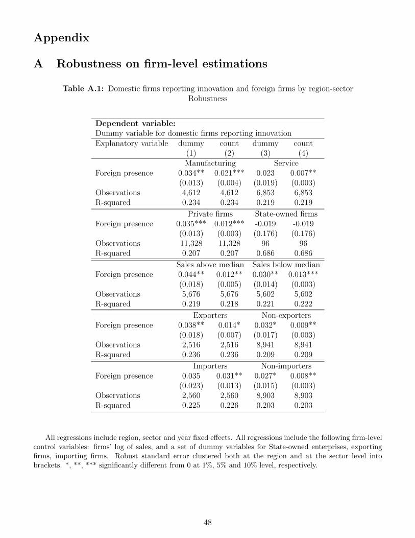
Appendix

A Robustness on firm-level estimations

Table A.1: Domestic firms reporting innovation and foreign firms by region-sectorRobustness

Dependent variable:Dummy variable for domestic firms reporting innovationExplanatory variable dummy count dummy count

(1) (2) (3) (4)Manufacturing Service

Foreign presence 0.034** 0.021*** 0.023 0.007**(0.013) (0.004) (0.019) (0.003)

Observations 4,612 4,612 6,853 6,853R-squared 0.234 0.234 0.219 0.219

Private firms State-owned firmsForeign presence 0.035*** 0.012*** -0.019 -0.019

(0.013) (0.003) (0.176) (0.176)Observations 11,328 11,328 96 96R-squared 0.207 0.207 0.686 0.686

Sales above median Sales below medianForeign presence 0.044** 0.012** 0.030** 0.013***

(0.018) (0.005) (0.014) (0.003)Observations 5,676 5,676 5,602 5,602R-squared 0.219 0.218 0.221 0.222

Exporters Non-exportersForeign presence 0.038** 0.014* 0.032* 0.009**

(0.018) (0.007) (0.017) (0.003)Observations 2,516 2,516 8,941 8,941R-squared 0.236 0.236 0.209 0.209

Importers Non-importersForeign presence 0.035 0.031** 0.027* 0.008**

(0.023) (0.013) (0.015) (0.003)Observations 2,560 2,560 8,903 8,903R-squared 0.225 0.226 0.203 0.203

All regressions include region, sector and year fixed effects. All regressions include the following firm-levelcontrol variables: firms’ log of sales, and a set of dummy variables for State-owned enterprises, exportingfirms, importing firms. Robust standard error clustered both at the region and at the sector level intobrackets. *, **, *** significantly different from 0 at 1%, 5% and 10% level, respectively.

48

B Model’s derivations

Labor market clearing. We derive the labor market clearing condition in the West as

`W =

∫ωW

aW q(ω, t)pW (−σ) c

P (t)1−σ dω +

∫ 1

0

IW

AWX(t)

L(t)dω

=( σ

σ − 1

)−σaW (1−σ) c

P (t)1−σQW (t) +

IW 2κ

γW. (42)

where Q(t) =∫ 1

0 q(ω, t)dω and QW (t) =∫ωW q(ω, t)dω. Also, QE(t) =

∫ωE q(ω, t)dω, QM (t) =

∫ωM q(ω, t)dω

and Q(t) = QW (t) +QE(t) +QM (t). In the East we obtain,

1− `W =

∫ωM

aMq(ω, t)pM(−σ) c

P (t)1−σ dω +

∫ωEaEq(ω, t)pE(−σ) c

P (t)1−σ dω

+

∫ωW

IM

AMX(t)

L(t)dω +

∫ωE+ωM

IE

AEX(t)

L(t)dω

=( σ

σ − 1

)−σaM(1−σ)wE(−σ) c

P (t)1−σQM (t) +

( σ

σ − 1

)−σaE(1−σ)wE(−σ) c

P (t)1−σQE(t)

+IM2κ

γMQW (t)

Q(t)+IE2κ

γE. (43)

Assets. Using the free entry conditions, we can derive the per capita assets of the two countries as

AW =

∫ωW+ωM

vW (ω)

LW (t)dω

=

∫ωW

(1− sW )2κ

γW `Wq(ω, t)

Q(t)dω +

∫ωM

(1− sW )2κ

γW `Wq(ω, t)

Q(t)dω

= (1− sW )2κ

γW `W(qW (t) + qM (t)), (44)

in the West, and similarly for the East

AE =

∫ωE

vE(ω)

LE(t)dω +

∫ωM

vM (ω)− vW (ω)

LE(t)dω

=

∫ωE

(1− sE)wE2κ

γE(1− `W )

q(ω, t)

QE+M (t)dω +

∫ωM

(1− sE)wE2κ

γM (1− `W )

q(ω, t)

Q(t)dω

= (1− sE)wE2κ

γE(1− `W )

qE(t)

qE(t) + qM (t)+ (1− sE)wE

2κ

γM (1− `W )qM (t). (45)

Expenditures. Substituting the two conditions above in the expressions for per-capita consumer expen-diture (25) and (27) we obtain the steady-state per capita consumption as

cW = 1 + (ρ− n)(1− sW )2κ

γW `W(qW (t) + qM (t))

−∫ω

sW IW2κ

γW `Wq(ω, t)

Q(t)dω

= 1 + (ρ− n)(1− sW )2κ

γW `W(qW (t) + qM (t))− sW IW 2κ

γW `W, (46)

49

for the West, and similarly for the East

cE = wE + (ρ− n)

((1− sE)wE

2κ

γE(1− `W )

qE(t)

qE(t) + qM (t)+ (1− sE)wE

2κ

γM (1− `W )qM (t)

)−

∫ωM+ωE

sEIEwE2κ

γE(1− `W )

q(ω, t)

QM+E(t)dω −

∫ωW

sEIMwE2κ

γM (1− `W )

q(ω, t)

Q(t)dω (47)

= wE[1 + (ρ− n)(1− sE)

2κ

1− `W

(1

γEqE(t)

qE(t) + qM (t)+qM (t)

γM

)− sE 2κ

1− `W

(IE

γE+IMqW (t)

γM

)].

Quality aggregates. The average quality index Q(t) equals the sum of the sectoral quality aggretates

Q(t) =

∫ωW

q(ω, t)dω +

∫ωEq(ω, t)dω +

∫ωM

q(ω, t)dω

= QW (t) +QE(t) +QM (t), (48)

which gives the condition1 = qW (t) + qE(t) + qM (t).

The quality aggregate in the West changes due to quality upgrades of Western products, leadership takeoverfrom the East and the multinationals and due to the transfer of production to subsidiary firms in the East.The following expression describes the evolution of QW , as a result of innovation and production transfers

QW (t) =

∫ωW

[λ(σ−1)(j(ω,t)+1) − λ(σ−1)j(ω,t)]IWdω +

∫ωEλ(σ−1)(j(ω,t)+1)IWdω

+

∫ωM

λ(σ−1)(j(ω,t)+1)IWdω −∫ωW

λ(σ−1)j(ω,t)IMdω,

which givesQW (t) = (λσ−1 − 1)IWQW (t) + λσ−1IW (QE(t) +QM (t))− IMQW (t). (49)

Similarly, for the aggregate quality in the East and multinationals’ production,

QE(t) =

∫ωE

[λ(σ−1)(j(ω,t)+1) − λ(σ−1)j(ω,t)]IEdω +

∫ωM

λ(σ−1)(j(ω,t)+1)IEdω

−∫ωEλ(σ−1)j(ω,t)IWdω

= (λσ−1 − 1)IEQE(t) + λσ−1IEQM (t)− IWQE(t), (50)

QM (t) =

∫ωW

λ(σ−1)j(ω,t)IMdω −∫ωM

λ(σ−1)j(ω,t)IWdω

−∫ωM

λ(σ−1)j(ω,t)IEdω

= IMQW (t)− (IW + IE)QM (t). (51)

Invariance of industry composition in any steady-state equilibrium requires that the growth rates of theaverage quality Q and its components (quality aggregates) must be constant and equal to each other. Theaverage product quality af all the production in the East is given by

QEM (t) = QE(t) +QM (t),

and therefore QEM evolves according to

QEM (t) = QE(t) + QM (t) = IMQW (t)− IW (QE(t) +QM (t)) + (λσ−1 − 1)IEQEM .

50

Equating the growth of quality aggregates in the West and in the East, QW (t)

QW (t)= QEM (t)

QEM (t), equation (17) is

obtainedλσ−1IW qW (t)−1 = IM

(qM (t) + qE(t)

)−1+ (λσ−1 − 1)IE .

Similarly, the growth rate of quality aggregates of the Eastern firms and the multinationals has to be the

same in a steady-state equilibrium, QE(t)QE(t)

= QM (t)QM (t)

, which yields the condition (18) as

qW (t)

qM (t) + qE(t)= λσ−1 I

E

IMqM (t)

qE(t)

Finally, adding (49), (50) and (51) and dividing by Q(t) we obtain equation (19).

Solving the model. Combining the arbitrage conditions for the West and the East (14 and 15) gives

wE(t)σ =

(aE

aW

)1−σ γE

γW1− sW

1− sEρ+ IW − n+ g

ρ+ IW + IE − n+ g(qE(t) + qM (t)) (52)

Combining the arbitrage conditions for the East and the multinationals (15 and 16) we obtain

wE(t)σ−1 =

[(aM

aE

)1−σ− γE

γM(qE(t) + qM (t))

](aE

aW

)1−σ ρ+ IW − n+ g

ρ+ IW + IE − n+ g. (53)

Note that equations 52 and 53 solve for the relative wage or for the relative quality in the West, i.e.

wE(t) =

[(aM

aE

)1−σ− γE

γM(qE(t) + qM (t))

]−1 γE

γW1− sW

1− sE(qE(t) + qM (t)), (54)

or

qW (t) = 1−[(wE)−1 +

γW

γM1− sE

1− sW

]−1(aMaE

)1−σ γW

γE1− sE

1− sW. (55)

Combining the arbitrage and the labor market clearing conditions for the West (14 and 42) equationbelow follows

`W = (σ − 1)(1− sW )2κ

γWqW (t)(ρ+ IW − n+ g) + IW

2κ

γW(56)

Combining the arbitrage and the labor market conditions for the East (15 and 43) equation below is derived

1− `W =

[(aM

aE

)1−σ qM (t)

1− qW (t)+

qE(t)

1− qW (t)

](ρ+ IW + IE − n+ g)(σ − 1)

(1− sE)2κ

γE

+ IM2κ

γMqW (t) + IE

2κ

γE. (57)

Finally, using qW+ qE +qM=1, conditions on quality aggregates evolution and the growth rate ofaverage quality Q(t) (17, 18 and 19) become

λσ−1IW qW (t)−1 = IM(1− qW (t))−1 + (λσ−1 − 1)IE, (58)

qW (t)

1− qW (t)= λσ−1 I

E

IMqM(t)

qE(t), (59)

(λσ−1 − 1)[IW + (1− qW (t))IE

]= g. (60)

Equations 52, 55, 56, 57, 58, 59 and 60 constitute a system of 7 equations endogenous in IW , IE, IM , wE

wW, g, Q

W (t)Q(t)

and QE(t)Q(t)

which solves for these variables.

51

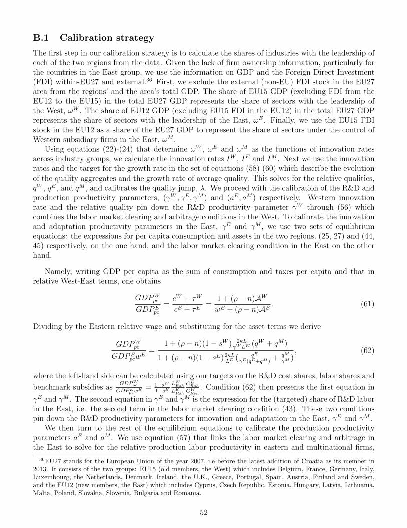
B.1 Calibration strategy

The first step in our calibration strategy is to calculate the shares of industries with the leadership ofeach of the two regions from the data. Given the lack of firm ownership information, particularly forthe countries in the East group, we use the information on GDP and the Foreign Direct Investment(FDI) within-EU27 and external.36 First, we exclude the external (non-EU) FDI stock in the EU27area from the regions’ and the area’s total GDP. The share of EU15 GDP (excluding FDI from theEU12 to the EU15) in the total EU27 GDP represents the share of sectors with the leadership ofthe West, ωW . The share of EU12 GDP (excluding EU15 FDI in the EU12) in the total EU27 GDPrepresents the share of sectors with the leadership of the East, ωE. Finally, we use the EU15 FDIstock in the EU12 as a share of the EU27 GDP to represent the share of sectors under the control ofWestern subsidiary firms in the East, ωM .

Using equations (22)-(24) that determine ωW , ωE and ωM as the functions of innovation ratesacross industry groups, we calculate the innovation rates IW , IE and IM . Next we use the innovationrates and the target for the growth rate in the set of equations (58)-(60) which describe the evolutionof the quality aggregates and the growth rate of average quality. This solves for the relative qualities,qW , qE, and qM , and calibrates the quality jump, λ. We proceed with the calibration of the R&D andproduction productivity parameters, (γW , γE, γM) and (aE, aM) respectively. Western innovationrate and the relative quality pin down the R&D productivity parameter γW through (56) whichcombines the labor market clearing and arbitrage conditions in the West. To calibrate the innovationand adaptation productivity parameters in the East, γE and γM , we use two sets of equilibriumequations: the expressions for per capita consumption and assets in the two regions, (25, 27) and (44,45) respectively, on the one hand, and the labor market clearing condition in the East on the otherhand.

Namely, writing GDP per capita as the sum of consumption and taxes per capita and that inrelative West-East terms, one obtains

GDPWpc

GDPEpc

=cW + τW

cE + τE=

1 + (ρ− n)AW

wE + (ρ− n)AE. (61)

Dividing by the Eastern relative wage and substituting for the asset terms we derive

GDPWpc

GDPEpcw

E=

1 + (ρ− n)(1− sW ) 2κLγWLW

(qW + qM)

1 + (ρ− n)(1− sE)2κLLE

( qE

γE(qE+qM )+ qM

γM), (62)

where the left-hand side can be calculated using our targets on the R&D cost shares, labor shares and

benchmark subsidies asGDPWpcGDPEpcw

E = 1−sW1−sE

LWRshLERsh

CERshCWRsh

. Condition (62) then presents the first equation in

γE and γM . The second equation in γE and γM is the expression for the (targeted) share of R&D laborin the East, i.e. the second term in the labor market clearing condition (43). These two conditionspin down the R&D productivity parameters for innovation and adaptation in the East, γE and γM .

We then turn to the rest of the equilibrium equations to calibrate the production productivityparameters aE and aM . We use equation (57) that links the labor market clearing and arbitrage inthe East to solve for the relative production labor productivity in eastern and multinational firms,

36EU27 stands for the European Union of the year 2007, i.e before the latest addition of Croatia as its member in2013. It consists of the two groups: EU15 (old members, the West) which includes Belgium, France, Germany, Italy,Luxembourg, the Netherlands, Denmark, Ireland, the U.K., Greece, Portugal, Spain, Austria, Finland and Sweden,and the EU12 (new members, the East) which includes Cyprus, Czech Republic, Estonia, Hungary, Latvia, Lithuania,Malta, Poland, Slovakia, Slovenia, Bulgaria and Romania.

52

aM

aE. This ratio is then used in (54) which combines the three arbitrage conditions to solve for the

eastern relative wage. Finally, we use the relative wage in any of the arbitrage conditions (52 or 53)to determine the production labor productivity in the eastern firms (aE), and consequently the onein the multinational firms as well (aM). Although we are not targeting the relative wage of 0.6 thatwe observe in the data, the wage resulting from our benchmark simulation is 0.45 and it satisfies the“product cycle “ conditions expressed in section 3.2.

53

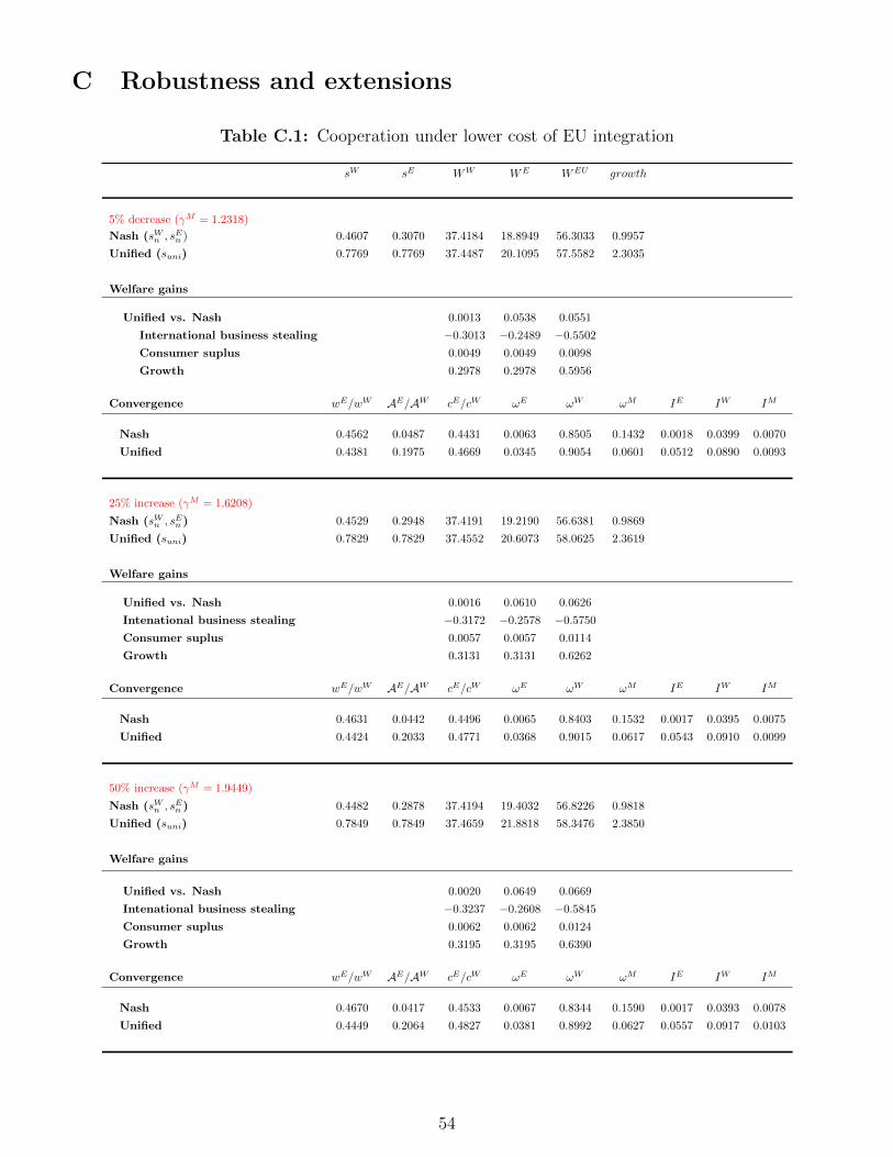
C Robustness and extensions

Table C.1: Cooperation under lower cost of EU integration

sW sE WW WE WEU growth

5% decrease (γM = 1.2318)

Nash (sWn , sEn ) 0.4607 0.3070 37.4184 18.8949 56.3033 0.9957

Unified (suni) 0.7769 0.7769 37.4487 20.1095 57.5582 2.3035

Welfare gains

Unified vs. Nash 0.0013 0.0538 0.0551

International business stealing −0.3013 −0.2489 −0.5502

Consumer suplus 0.0049 0.0049 0.0098

Growth 0.2978 0.2978 0.5956

Convergence wE/wW AE/AW cE/cW ωE ωW ωM IE IW IM

Nash 0.4562 0.0487 0.4431 0.0063 0.8505 0.1432 0.0018 0.0399 0.0070

Unified 0.4381 0.1975 0.4669 0.0345 0.9054 0.0601 0.0512 0.0890 0.0093

25% increase (γM = 1.6208)

Nash (sWn , sEn ) 0.4529 0.2948 37.4191 19.2190 56.6381 0.9869

Unified (suni) 0.7829 0.7829 37.4552 20.6073 58.0625 2.3619

Welfare gains

Unified vs. Nash 0.0016 0.0610 0.0626

Intenational business stealing −0.3172 −0.2578 −0.5750

Consumer suplus 0.0057 0.0057 0.0114

Growth 0.3131 0.3131 0.6262

Convergence wE/wW AE/AW cE/cW ωE ωW ωM IE IW IM

Nash 0.4631 0.0442 0.4496 0.0065 0.8403 0.1532 0.0017 0.0395 0.0075

Unified 0.4424 0.2033 0.4771 0.0368 0.9015 0.0617 0.0543 0.0910 0.0099

50% increase (γM = 1.9449)

Nash (sWn , sEn ) 0.4482 0.2878 37.4194 19.4032 56.8226 0.9818

Unified (suni) 0.7849 0.7849 37.4659 21.8818 58.3476 2.3850

Welfare gains

Unified vs. Nash 0.0020 0.0649 0.0669

Intenational business stealing −0.3237 −0.2608 −0.5845

Consumer suplus 0.0062 0.0062 0.0124

Growth 0.3195 0.3195 0.6390

Convergence wE/wW AE/AW cE/cW ωE ωW ωM IE IW IM

Nash 0.4670 0.0417 0.4533 0.0067 0.8344 0.1590 0.0017 0.0393 0.0078

Unified 0.4449 0.2064 0.4827 0.0381 0.8992 0.0627 0.0557 0.0917 0.0103

54

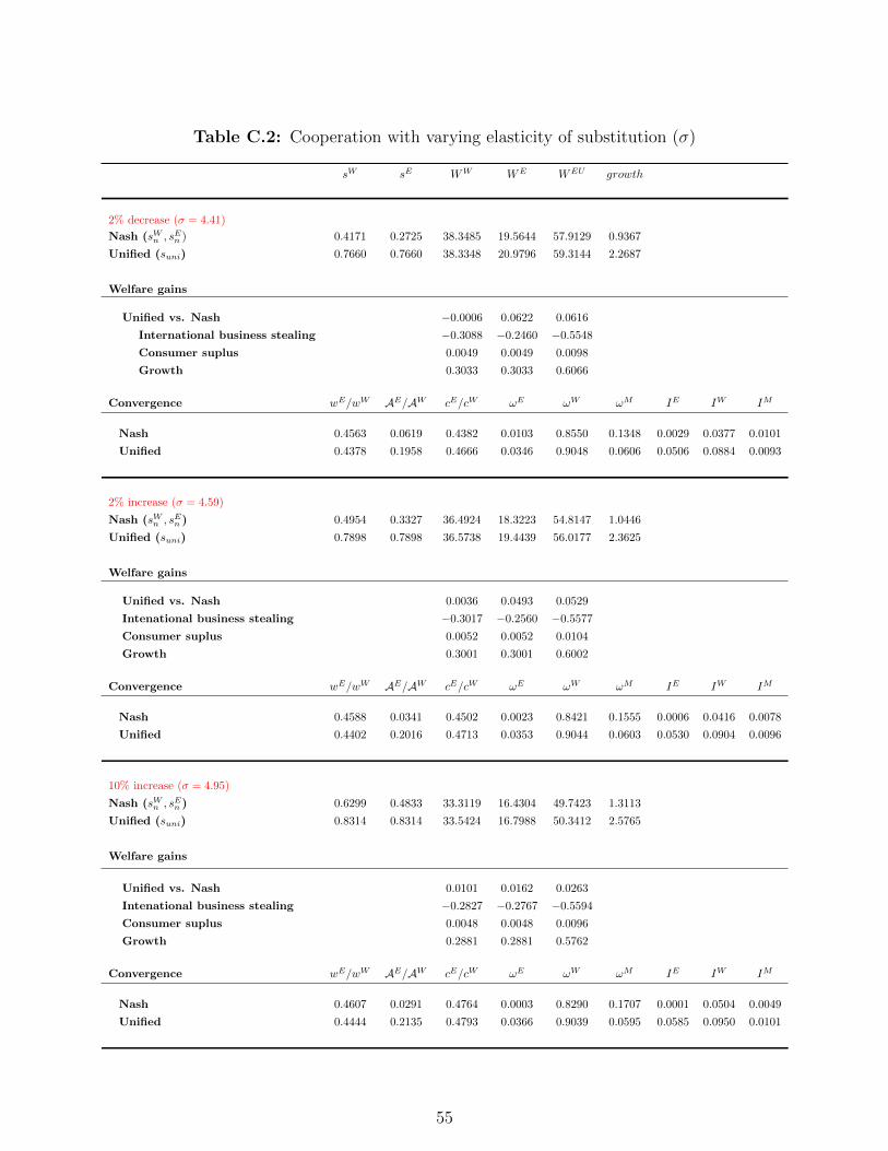
Table C.2: Cooperation with varying elasticity of substitution (σ)

sW sE WW WE WEU growth

2% decrease (σ = 4.41)

Nash (sWn , sEn ) 0.4171 0.2725 38.3485 19.5644 57.9129 0.9367

Unified (suni) 0.7660 0.7660 38.3348 20.9796 59.3144 2.2687

Welfare gains

Unified vs. Nash −0.0006 0.0622 0.0616

International business stealing −0.3088 −0.2460 −0.5548

Consumer suplus 0.0049 0.0049 0.0098

Growth 0.3033 0.3033 0.6066

Convergence wE/wW AE/AW cE/cW ωE ωW ωM IE IW IM

Nash 0.4563 0.0619 0.4382 0.0103 0.8550 0.1348 0.0029 0.0377 0.0101

Unified 0.4378 0.1958 0.4666 0.0346 0.9048 0.0606 0.0506 0.0884 0.0093

2% increase (σ = 4.59)

Nash (sWn , sEn ) 0.4954 0.3327 36.4924 18.3223 54.8147 1.0446

Unified (suni) 0.7898 0.7898 36.5738 19.4439 56.0177 2.3625

Welfare gains

Unified vs. Nash 0.0036 0.0493 0.0529

Intenational business stealing −0.3017 −0.2560 −0.5577

Consumer suplus 0.0052 0.0052 0.0104

Growth 0.3001 0.3001 0.6002

Convergence wE/wW AE/AW cE/cW ωE ωW ωM IE IW IM

Nash 0.4588 0.0341 0.4502 0.0023 0.8421 0.1555 0.0006 0.0416 0.0078

Unified 0.4402 0.2016 0.4713 0.0353 0.9044 0.0603 0.0530 0.0904 0.0096

10% increase (σ = 4.95)

Nash (sWn , sEn ) 0.6299 0.4833 33.3119 16.4304 49.7423 1.3113

Unified (suni) 0.8314 0.8314 33.5424 16.7988 50.3412 2.5765

Welfare gains

Unified vs. Nash 0.0101 0.0162 0.0263

Intenational business stealing −0.2827 −0.2767 −0.5594

Consumer suplus 0.0048 0.0048 0.0096

Growth 0.2881 0.2881 0.5762

Convergence wE/wW AE/AW cE/cW ωE ωW ωM IE IW IM

Nash 0.4607 0.0291 0.4764 0.0003 0.8290 0.1707 0.0001 0.0504 0.0049

Unified 0.4444 0.2135 0.4793 0.0366 0.9039 0.0595 0.0585 0.0950 0.0101

55

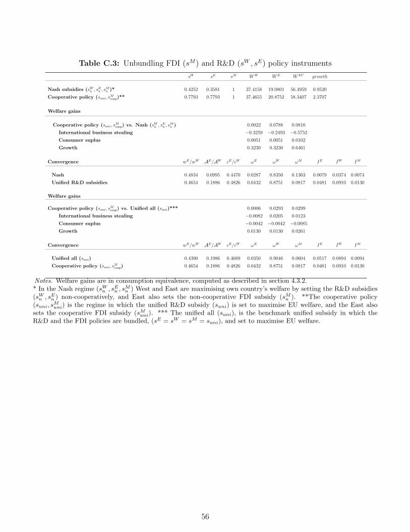
Table C.3: Unbundling FDI (sM) and R&D (sW , sE) policy instruments

sW sE sM WW WE WEU growth

Nash subsidies (sWn , sEn , s

Mn )* 0.4252 0.3581 1 37.4158 19.0801 56.4959 0.9520

Cooperative policy (suni, sMcoop)** 0.7793 0.7793 1 37.4655 20.8752 58.3407 2.3707

Welfare gains

Cooperative policy (suni, sMcoop) vs. Nash (sWn , s

En , s

Mn ) 0.0022 0.0788 0.0810

International business stealing −0.3259 −0.2493 −0.5752

Consumer suplus 0.0051 0.0051 0.0102

Growth 0.3230 0.3230 0.6461

Convergence wE/wW AE/AW cE/cW ωE ωW ωM IE IW IM

Nash 0.4834 0.0995 0.4470 0.0287 0.8350 0.1363 0.0079 0.0374 0.0074

Unified R&D subsidies 0.4654 0.1886 0.4826 0.0432 0.8751 0.0817 0.0481 0.0910 0.0130

Welfare gains

Cooperative policy (suni, sMcoop) vs. Unified all (suni)*** 0.0006 0.0293 0.0299

International business stealing −0.0082 0.0205 0.0123

Consumer suplus −0.0042 −0.0042 −0.0085

Growth 0.0130 0.0130 0.0261

Convergence wE/wW AE/AW cE/cW ωE ωW ωM IE IW IM

Unified all (suni) 0.4390 0.1986 0.4689 0.0350 0.9046 0.0604 0.0517 0.0894 0.0094

Cooperative policy (suni, sMcoop) 0.4654 0.1886 0.4826 0.0432 0.8751 0.0817 0.0481 0.0910 0.0130

Notes. Welfare gains are in consumption equivalence, computed as described in section 4.3.2.* In the Nash regime (sWn , s

En , s

Mn ) West and East are maximising own country’s welfare by setting the R&D subsidies

(sWn , sEn ) non-cooperatively, and East also sets the non-cooperative FDI subsidy (sMn ). **The cooperative policy

(suni, sMuni) is the regime in which the unified R&D subsidy (suni) is set to maximise EU welfare, and the East also

sets the cooperative FDI subsidy (sMuni). *** The unified all (suni), is the benchmark unified subsidy in which theR&D and the FDI policies are bundled, (sE = sW = sM = suni), and set to maximise EU welfare.

56

C.1 Alternative assets allocation

In the alternative specification we assume that Western consumers finance both the innovative R&Din the West and the adaptive R&D for the transfer of production to the East, and thus recieve,in the form of dividends, the profits of firms operating in the West and increased profits from themultinational operations in the East. The East, on the other hand, finances only the innovative R&Dof the local firms and thus receive the profits of the eastern leaders.

Therefore, using the free entry conditions, we can derive the total per-capita assets of the tworegions as

AW =

∫ωW

vW (ω)

LW (t)dω +

∫ωM

vM(ω)

LW (t)dω =

∫ωW+ωM

vW (ω)

LW (t)dω +

∫ωM

(vM(ω)− vW (ω))

LW (t)dω

=

∫ωW+ωM

(1− sW )2κ

γW `Wq(ω, t)

Q(t)dω +

∫ωM

(1− sE)wE2κ

γM`Wq(ω, t)

Q(t)dω

= (1− sW )2κ

γW `W(qW (t) + qM(t)) + (1− sE)wE

2κ

γM`WqM(t), (63)

in the West, and similarly for the East

AE =

∫ωE

vE

LE(t)(ω)dω

=

∫ωE

(1− sE)wE2κ

γE(1− `W )

q(ω, t)

QE+M(t)dω

= (1− sE)wE2κ

γE(1− `W )

qE(t)

qE(t) + qM(t). (64)

Substituting the two conditions above in the expressions for per-capita consumer expenditure weobtain the steady-state per-capita consumption as

cW = 1 + (ρ− n)

((1− sW )

2κ

γW `W(qW (t) + qM (t)) + (1− sE)wE

2κ

γM `WqM (t)

)−

∫ω

sW IW2κ

γW `Wq(ω, t)

Q(t)dω

= 1 + (ρ− n)(1− sW )2κ

`W

(qW (t) + qM (t)

γW+ wE

qM (t)

γM

)− sW IW 2κ

γW `W, (65)

for the West, and similarly for the East

cE = wE(

1 + (ρ− n)(1− sE)2κ

γE(1− `W )

qE(t)

qE(t) + qM (t)

−∫

ωM+ωE

sEIE2κ

γE(1− `W )

q(ω, t)

QM+E(t)dω −

∫ωW

sEIM2κ

γM (1− `W )

q(ω, t)

Q(t)dω

)

= wE(

1 + (ρ− n)(1− sE)2κ

γE(1− `W )

qE(t)

qE(t) + qM (t)− sE 2κ

1− `W

[IE

γE+IM

γMqW (t)

]). (66)

Compared to the main specification in the text, the difference in the global distribution of assets

57

comes from a different allocation of the additional assets value created in the sectors that transferproduction from the West to the East. This is represented by the last term in the expression foreastern assets in the main specification (equation 45), which now becomes a part of western assetsin the alternative specification with western financing of the transfer (last term in the expression forwestern assets, equation 63). This change has an effect on the consumption expenditure channel inour welfare analysis, but has no implications on the change in total welfare of each region with anincrease in subsidies.

For illustration, we present the numerical simulation of the Western R&D subsidy effects in FiguresC.1 and C.2. An increase in Western subsidy produces the same effects on the innovation rates andgeographical distribution of sectoral leadership as in the main specification. Due to a strong increasein innovation in all sectors in the West the growth component of welfare is higher. In the West,consumption expenditure now increases with subsidies due to additional assets value coming fromthe increased production transfer, now financed and appropriated by the West. However, the effect isnot strong enough to compensate for the higher tax burden of raised subsidies and the consumptioncomponent of the welfare falls. On the other hand, the price index falls with more production done bythe multinational firms in the East which contributes positively to both regions’ welfare. As before,the total welfare in the West rises.

In the East, the value of assets falls with Western R&D subsidy, not only due to a loss in sectoralleadership, but also due to the loss of additional sectoral profits of multinational subsidiaries which arenow appropriated by the West. The consumption expenditure channel is reduced, but this negativeeffect is compensated for by the price index channel, and the rise in the global growth rate. Therefore,the welfare in the East increases.

58

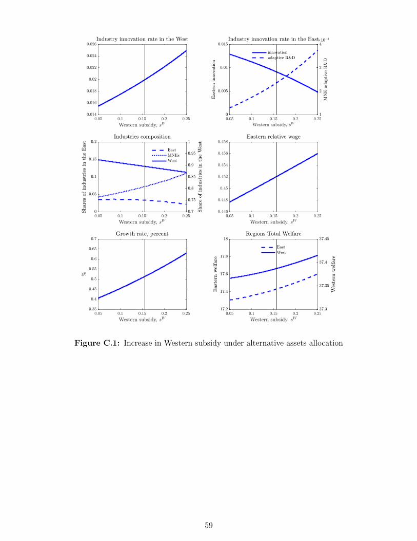
Figure C.1: Increase in Western subsidy under alternative assets allocation

59

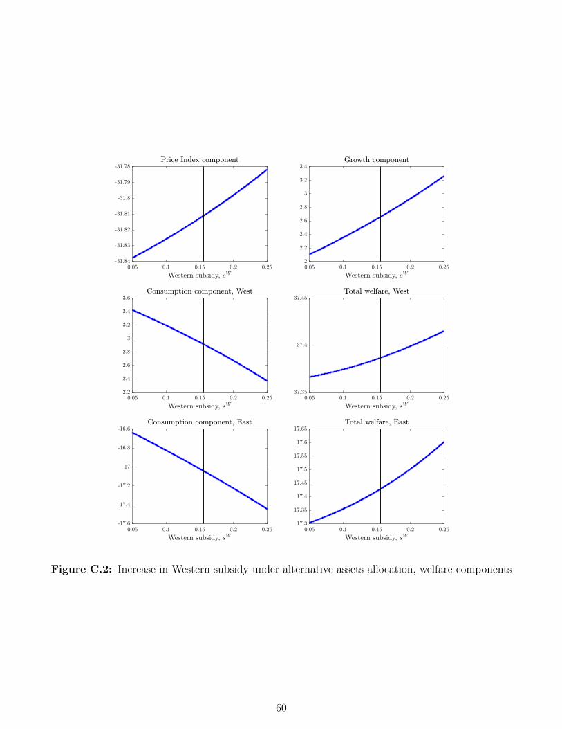
Figure C.2: Increase in Western subsidy under alternative assets allocation, welfare components

60

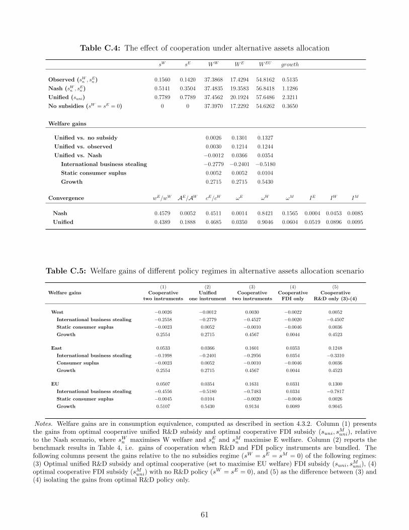
Table C.4: The effect of cooperation under alternative assets allocation

sW sE WW WE WEU growth

Observed (sWn , sEn ) 0.1560 0.1420 37.3868 17.4294 54.8162 0.5135

Nash (sWn , sEn ) 0.5141 0.3504 37.4835 19.3583 56.8418 1.1286

Unified (suni) 0.7789 0.7789 37.4562 20.1924 57.6486 2.3211

No subsidies (sW = sE = 0) 0 0 37.3970 17.2292 54.6262 0.3650

Welfare gains

Unified vs. no subsidy 0.0026 0.1301 0.1327

Unified vs. observed 0.0030 0.1214 0.1244

Unified vs. Nash −0.0012 0.0366 0.0354

International business stealing −0.2779 −0.2401 −0.5180

Static consumer suplus 0.0052 0.0052 0.0104

Growth 0.2715 0.2715 0.5430

Convergence wE/wW AE/AW cE/cW ωE ωW ωM IE IW IM

Nash 0.4579 0.0052 0.4511 0.0014 0.8421 0.1565 0.0004 0.0453 0.0085

Unified 0.4389 0.1888 0.4685 0.0350 0.9046 0.0604 0.0519 0.0896 0.0095

Table C.5: Welfare gains of different policy regimes in alternative assets allocation scenario

(1) (2) (3) (4) (5)Welfare gains Cooperative Unified Cooperative Cooperative Cooperative

two instruments one instrument two instruments FDI only R&D only (3)-(4)

West −0.0026 −0.0012 0.0030 −0.0022 0.0052

International business stealing −0.2558 −0.2779 −0.4527 −0.0020 −0.4507

Static consumer suplus −0.0023 0.0052 −0.0010 −0.0046 0.0036

Growth 0.2554 0.2715 0.4567 0.0044 0.4523

East 0.0533 0.0366 0.1601 0.0353 0.1248

International business stealing −0.1998 −0.2401 −0.2956 0.0354 −0.3310

Consumer suplus −0.0023 0.0052 −0.0010 −0.0046 0.0036

Growth 0.2554 0.2715 0.4567 0.0044 0.4523

EU 0.0507 0.0354 0.1631 0.0331 0.1300

International business stealing −0.4556 −0.5180 −0.7483 0.0334 −0.7817

Static consumer suplus −0.0045 0.0104 −0.0020 −0.0046 0.0026

Growth 0.5107 0.5430 0.9134 0.0089 0.9045

Notes. Welfare gains are in consumption equivalence, computed as described in section 4.3.2. Column (1) presentsthe gains from optimal cooperative unified R&D subsidy and optimal cooperative FDI subsidy (suni, s

Muni), relative

to the Nash scenario, where sWn maximises W welfare and sEn and sMn maximise E welfare. Column (2) reports thebenchmark results in Table 4, i.e. gains of cooperation when R&D and FDI policy instruments are bundled. Thefollowing columns present the gains relative to the no subsidies regime (sW = sE = sM = 0) of the following regimes:(3) Optimal unified R&D subsidy and optimal cooperative (set to maximise EU welfare) FDI subsidy (suni, s

Muni), (4)

optimal cooperative FDI subsidy (sMuni) with no R&D policy (sW = sE = 0), and (5) as the difference between (3) and(4) isolating the gains from optimal R&D policy only.

61

Table C.6: Unbundling FDI (sM) and R&D (sW , sE) policy instruments in the alternative assetsallocation scenario

sW sE sM WW WE WEU growth

Benchmark FDI subsidy

Observed R&D subsidies (sWn , sEn ) 0.1560 0.1420 0.1420 37.3868 17.4294 54.8162 0.5135

Nash R&D subsidies (sWn , sEn ) 0.5460 0.3748 0.1420 37.5100 19.5704 57.0804 1.2062

No R&D subsidies (sW = sE = 0) 0 0 0.1420 37.3920 17.3391 54.7311 0.3672

Optimal FDI subsidy

Observed R&D subsidies (sWn , sEn ) 0.1560 0.1420 1 37.3444 18.1926 55.5370 0.5361

Nash subsidies (sWn , sEn , s

Mn )* 0.5628 0.3916 0 37.5256 19.6618 57.1873 1.2493

Unified R&D subsidies (suni)** 0.7793 0.7793 1 37.4655 20.8752 58.3407 2.3707

No R&D subsidies (sW = sE = 0) 0 0 1 37.3477 18.0324 55.3801 0.3845

Welfare gains

Unified R&D subsidies vs. Nash −0.0026 0.0533 0.0507

International business stealing −0.2558 −0.1998 −0.4556

Consumer suplus −0.0023 −0.0023 −0.0045

Growth 0.2554 0.2554 0.5107

Convergence wE/wW AE/AW cE/cW ωE ωW ωM IE IW IM

Nash 0.4407 0.0044 0.4563 0.0011 0.8605 0.1385 0.0004 0.0502 0.0081

Unified R&D subsidies 0.4654 0.1886 0.4826 0.0432 0.8751 0.0817 0.0481 0.0910 0.0130

Welfare gains

Unified R&D subsidies vs. Unified all*** 0.0004 0.0300 0.0304

International business stealing −0.0067 0.0229 0.0161

Consumer suplus −0.0043 −0.0043 −0.0085

Growth 0.0114 0.0114 0.0228

Convergence wE/wW AE/AW cE/cW ωE ωW ωM IE IW IM

Unified all subsidies 0.4389 0.1888 0.4685 0.0350 0.9046 0.0604 0.0519 0.0896 0.0095

Unified R&D subsidies 0.4654 0.1886 0.4826 0.0432 0.8751 0.0817 0.0481 0.0910 0.0130

* (sWn , sEn , s

Mn ) regime in which West and East are maximizing own country’s welfare by setting the non-cooperative

R&D subsidies (sWn , sEn ) , while East also sets the non-cooperative FDI subsidy (sMn )

**(suni, sMuni) regime in which West and East are maximizing the total EU welfare by setting the unified cooperative

R&D subsidy (suni) , while East also sets the cooperative FDI subsidy (sMuni)***(suni) regime in which the R&D and the FDI policies are bundled, West and East are maximizing the total EUwelfare by setting the unified cooperative subsidy (suni) applying to both R&D and FDI policies.

62

CENTRE FOR ECONOMIC PERFORMANCE

Recent Discussion Papers

1639 Monica Langella

Alan Manning

Residential Mobility and Unemployment in

the UK

1638 Christos Genakos

Mario Pagliero

Competition and Pass-Through: Evidence

from Isolated Markets

1637 Holger Breinlich

Elsa Leromain

Dennis Novy

Thomas Sampson

Voting With Their Money: Brexit and

Outward Investment by UK Firms

1636 Maria Sanchez-Vidal Retail Shocks and City Structure

1635 Felipe Carozzi

Sefi Roth

Dirty Density: Air Quality and the Density of

American Cities

1634 Nicholas Bloom

John Van Reenen

Heidi Williams

A Toolkit of Policies to Promote Innovation

1633 Stephan E. Maurer

Ferdinand Rauch

Economic Geography Aspects of the Panama

Canal

1632 Nikhil Datta Willing to Pay for Security: A Discrete

Choice Experiment to Analyse Labour Supply

Preferences

1631 Gabriel M. Ahlfeldt

Volker Nitsch

Nicolai Wendland

Ease Versus Noise: Long-Run Changes in the

Value of Transport (Dis)amenities

1630 Grace Lordan

Alistair McGuire

Widening the High School Curriculum to

Include Soft Skill Training: Impacts on

Health, Behaviour, Emotional Wellbeing and

Occupational Aspirations

1629 Per-Anders Edin

Tiernan Evans

Georg Graetz

Sofia Hernnäs

Guy Michaels

Individual Consequences of Occupational

Decline

1628 Pawel Bukowski

Filip Novokmet

Between Communism and Capitalism: Long-

Term Inequality in Poland, 1892-2015

1627 Thomas Sampson Technology Gaps, Trade and Income

1626 Andrea Ichino

Martin Olsson

Barbara Petrongolo

Peter Skogman Thoursie

Economic Incentives, Home Production and

Gender Identity Norms

1625 Richard Murphy Why Unions Survive: Understanding How

Unions Overcome the Free-Rider Problem

1624 Natalie Chen

Wanyu Chung

Dennis Novy

Vehicle Currency Pricing and Exchange Rate

Pass-Through

1623 Michael Amior

Alan Manning

Commuting, Migration and Local Joblessness

1622 Rui Costa

Swati Dhingra

Stephen Machin

Trade and Worker Deskilling

1621 Jan-Emmanuel De Neve

Clement Imbert

Johannes Spinnewijn

Teodora Tsankova,

Maarten Luts

How to Improve Tax Compliance? Evidence

from Population-wide Experiments in

Belgium

The Centre for Economic Performance Publications Unit

Tel: +44 (0)20 7955 7673 Email info@cep.lse.ac.uk

Website: http://cep.lse.ac.uk Twitter: @CEP_LSE