Embed Size (px)
Citation preview
ISSN 2042-2695
CEP Discussion Paper No 1245
October 2013
What Predicts a Successful Life? A Life-Course Model of Well-Being
Richard Layard Andrew E. Clark
Francesca Cornaglia Nattavudh Powdthavee
James Vernoit
Abstract If policy-makers care about well-being, they need a recursive model of how adult life-satisfaction is predicted by childhood influences, acting both directly and (indirectly) through adult circumstances. We estimate such a model using the British Cohort Study (1970). The most powerful childhood predictor of adult life-satisfaction is the child’s emotional health. Next comes the child’s conduct. The least powerful predictor is the child’s intellectual development. This has obvious implications for educational policy. Among adult circumstances, family income accounts for only 0.5% of the variance of life-satisfaction. Mental and physical health are much more important. Keywords: Well-being, Life-satisfaction, Intervention, Model, Life-course, Emotional health, Conduct, Intellectual performance, Success JEL Classifications: A12; D60; H00; I31 This paper was produced as part of the Centre’s Well-Being Programme. The Centre for Economic Performance is financed by the Economic and Social Research Council. Acknowledgements We are extremely grateful for research assistance from Nele Warrinnier and Rachel Berner, for advice from Steve Pischke, and for comments from Michael Daly, Bruno Frey, Alissa Goodman, David Howdon, Stephen Jenkins, Kathy Kiernan, Grace Lordan, Andrew Oswald, Carol Propper and Marcus Richards. This research was supported by the UK Department for Work and Pensions, the U.S. National Institute of Aging (Grant No R01AG040640) and private donations. Richard Layard is Director of the Wellbeing Programme at the Centre for Economic Performance and Emeritus Professor of Economics, London School of Economics and Political Science. Andrew E. Clark is a Research Fellow at the Centre for Economic Performance, London School of Economics and Political Science and IZA. He is also a Research Professor at the Paris School of Economics. Francesca Cornaglia is a Research Associate at the Centre for Economic Performance, London School of Economics and Political Science and Lecturer in the School of Economics and Finance at Queen Mary University of London. Nattavudh Powdthavee is a Principal Research Fellow with the Wellbeing Programme at the Centre for Economic Performance, London School of Economics. He is also a Professorial Research Fellow at the Melbourne Institute of Applied Economics and Social Research. James Vernoit is a Research Assistant for the Well-Being Programme at the Centre for Economic Performance. Published by Centre for Economic Performance London School of Economics and Political Science Houghton Street London WC2A 2AE All rights reserved. No part of this publication may be reproduced, stored in a retrieval system or transmitted in any form or by any means without the prior permission in writing of the publisher nor be issued to the public or circulated in any form other than that in which it is published. Requests for permission to reproduce any article or part of the Working Paper should be sent to the editor at the above address. R. Layard, A.E. Clark, F. Cornaglia, N. Powdthavee and J. Vernoit, submitted 2013
“The ultimate purpose of economics, of course, is to understand and promote the
enhancement of well-being”.1 This sentiment, expressed in 2012 by the Chairman of the US
Federal Reserve, is of course directly in line with that of Adam Smith and the other founding
fathers of economics. What has been lacking is evidence of the determinants of well-being.
That situation is now changing. Cross-sectional data have been analysed for some decades,
and show the strong relation between current characteristics and well-being. But we also need
to know how those characteristics arose, if we want to decide at what point in the life-cycle
interventions would be most cost-effective.
So, if policy is to maximise well-being, the prerequisite is a model of the life-course
that captures in a quantitative way the relative impact of all the main influences upon
subsequent well-being. Separate studies of the effect of one variable at a time are of little use
in thinking about resource allocation. The effects have to be compared.
The need here is not unlike the need of macroeconomic policy for a working model of
the economy. So it is not surprising that the OECD, having developed an international
standard for the measurement of well-being,2 are calling for much more research to model
what determines it.
1. Why a Life-Course Model?
To be useful, a model must combine the two main strands in previous well-being
research. The first of these, pioneered by among others Campbell, Converse and Rodgers,
Diener, Kahneman, Oswald, Frey and Helliwell, has focussed on how well-being is affected
proximally by other adult outcomes. These include those that can be called ‘economic’
(income, employment, educational qualifications), those that are ‘social’ (family status,
criminality) and those that are ‘personal’ (physical and emotional health).3
The second strand of work so far has used cohort data to explore the distal influence of
childhood and adolescence upon adult well-being. This strand follows the earlier work of
economists such as Heckman and Smith4 on the lifetime determinants of earnings. But,
instead, it takes adult well-being as the outcome of interest. Recent leaders in this field of
work include Frijters, Johnston and Shields.5 But their work focusses exclusively on the well-
being outcome, and ignores the determination of other adult outcomes like income,
employment, family status, criminality and health, which then feed into well-being. Such an
approach could lead to an excessive focus on childhood and adolescence as determinants of
well-being, with little role left for policies relating to adult life.
1 Speech by Ben S. Bernanke to 32nd General Conference of the International Association for Research in
Income and Wealth, Cambridge, Massachusetts, 6th August 2012. 2 OECD (2013).
3 See for example, Campbell et al. (1976); Kahneman et al. (1999); Clark and Oswald (1994); Frey and Stutzer
(2002); and Helliwell (2003). Layard et al. (2012) summarise much of this research. 4 See for example Cunha and Heckman (2008); Cunha et al. (2010); Goodman et al. (2011).
5 Frijters et al. (2011), see also Richards and Huppert (2011) and Boyce et al. (2013). There is a considerable
earlier literature on the determinants of adult malaise e.g. Furstenberg and Kiernan (2001); Knapp et al. (2011a)
also examine effects on earnings and employment.
2
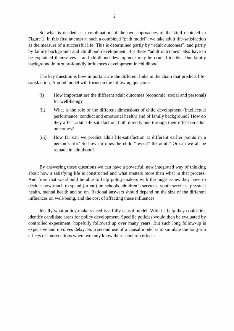
So what is needed is a combination of the two approaches of the kind depicted in
Figure 1. In this first attempt at such a combined “path model”, we take adult life-satisfaction
as the measure of a successful life. This is determined partly by “adult outcomes”, and partly
by family background and childhood development. But these “adult outcomes” also have to
be explained themselves – and childhood development may be crucial to this. Our family
background in turn profoundly influences development in childhood.
The key question is how important are the different links in the chain that predicts life-
satisfaction. A good model will focus on the following questions
(i) How important are the different adult outcomes (economic, social and personal)
for well-being?
(ii) What is the role of the different dimensions of child development (intellectual
performance, conduct and emotional health) and of family background? How do
they affect adult life-satisfaction, both directly and through their effect on adult
outcomes?
(iii) How far can we predict adult life-satisfaction at different earlier points in a
person’s life? So how far does the child “reveal” the adult? Or can we all be
remade in adulthood?
By answering these questions we can have a powerful, new integrated way of thinking
about how a satisfying life is constructed and what matters more than what in that process.
And from that we should be able to help policy-makers with the huge issues they have to
decide: how much to spend (or cut) on schools, children’s services, youth services, physical
health, mental health and so on. Rational answers should depend on the size of the different
influences on well-being, and the cost of affecting these influences.
Ideally what policy-makers need is a fully causal model. With its help they could first
identify candidate areas for policy development. Specific policies would then be evaluated by
controlled experiment, hopefully followed up over many years. But such long follow-up is
expensive and involves delay. So a second use of a causal model is to simulate the long-run
effects of interventions where we only know their short-run effects.
3
Fig. 1. A Model of Adult Life-Satisfaction
To develop a fully causal model will take years more of data-collection and research. In
particular it will be crucial to include genetic controls, since omitting variables of this kind
can exaggerate the extent to which earlier life determines later life.6 At the same time,
measurement error tends to underestimate the continuities, and better measures need to be
developed.
But in the meantime policy-making will continue. At present most of the policy debate
is conducted without reference to any quantitative evidence about what matters most for well-
being. It would be much better if it were informed by broad orders of magnitude from a
quantitative model, even if the model is more properly called predictive than causal. We have
to start somewhere and, as we shall see, even from a simple model, some striking conclusions
emerge.
6 See for example, De Neve et al. (2012).
Family
background
Child
characteristics
Adult
outcomes
‘Final outcome’
Economic
Psycho-social
Intellectual
performance
Good conduct
Emotional health
Income
Educational level
Employment
Conduct
Family status
Physical health
Emotional health
Adult
life-satisfaction
4
2. Our Model, Data and Methods
The model we develop is a recursive path model in which life-satisfaction at each age
can in principle depend on everything that happened before that.7 As shown in Figure 1,
antecedent conditions include seven adult state variables (Xi) that evolve throughout a
person’s adult life (income, educational level, employment, conduct, family status, physical
and emotional health) – or eight if we include life-satisfaction (X8). During childhood we
only have data on three of these characteristics: intellectual performance (corresponding to
‘qualifications’ in later life); conduct (continuing in later life); and emotional health
(continuing in later life).8 Thus for three of the Xi variables we have data for early life, while
for others the data start in adulthood. We also have data on the family background of the
individual, characterised by the family’s economic status (FE) and its psychosocial state (F
P).
To explain the evolution of all the Xi variables, we have a recursive or path model, in
which the value of each variable may in principle depend on everything that has gone before.
Thus
( ) (i = 1,…,8; all available t)
2.1. Variables
To estimate this model we use the British Cohort Study, which covers people born in
the second week of March, 1970. Well-being is measured by life-satisfaction at age 34. To
explain this we have adult outcome variables, three sets of childhood characteristics and the
characteristics of the family.
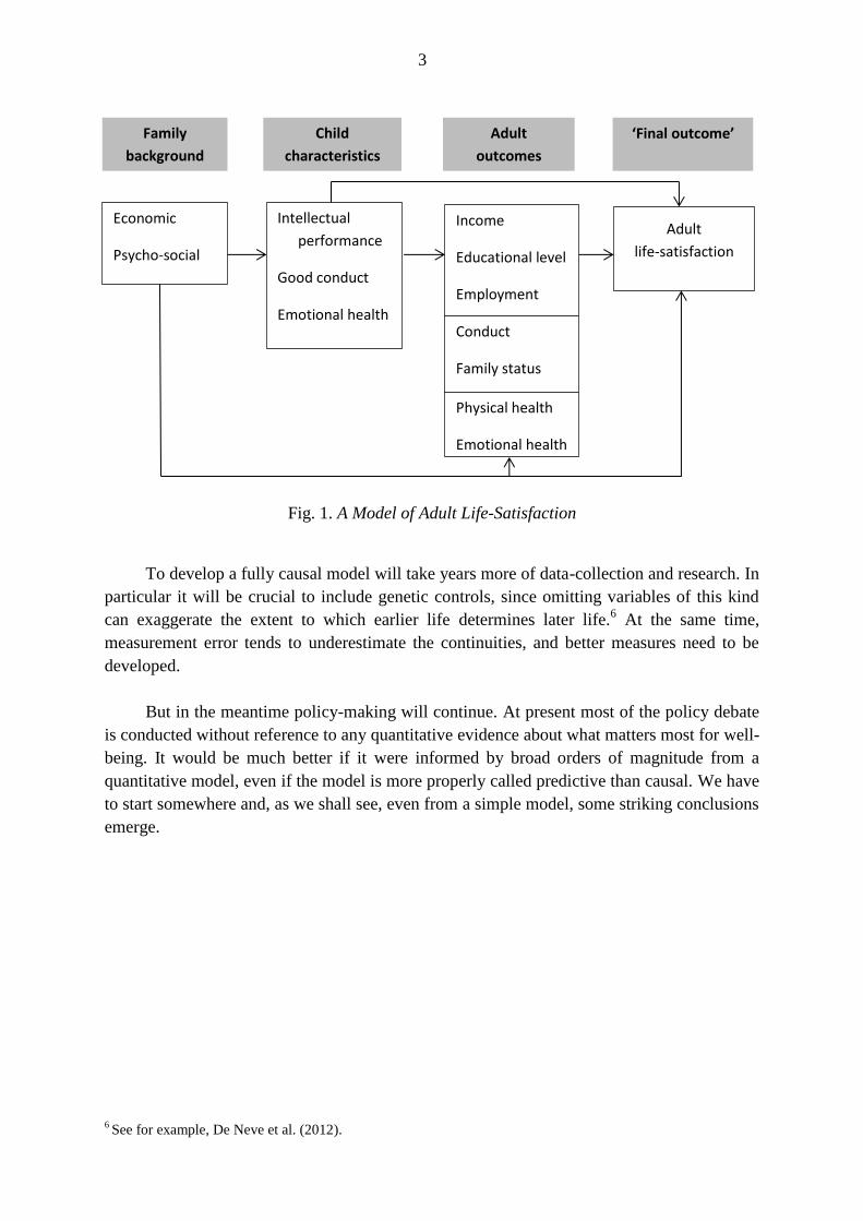
Specifically our adult outcomes are as shown in Figure 2. Note that we have measured
emotional health and self-perceived health at 26 rather than 34 so as to avoid any charge that
these are the same as life-satisfaction rather than predictors of it.
Emotional health and life-satisfaction are in fact very different, which is why life-
satisfaction is predicted by so many other influences as well. For life-satisfaction the question
is, “How dissatisfied or satisfied are you about the way your life has turned out so far?” For
adult emotional health we have 24 yes/no questions relating to tiredness, depression, worry,
irrational fear, rage, irritation, tension and psychosomatic symptoms (see Appendix B). These
are very different from the life-satisfaction question.
7 For this type of structural equation modelling, see for example Goodman et al. (2011) and Schoon et al. (2012).
8 Unfortunately the BCS includes no measure of physical health in childhood, but childhood physical health
probably accounts for a relatively small part of the variance of adult outcomes.
5
Economic Log income (equivalised) at 34
Educational achievement by 34
Employed (measured as not
employed)
at 34
Social Good conduct (= -no. of crimes) at 16-34
Has a partner at 34
Personal Self-perceived health
Emotional health
at 26
at 26
Fig. 2. Adult Outcomes
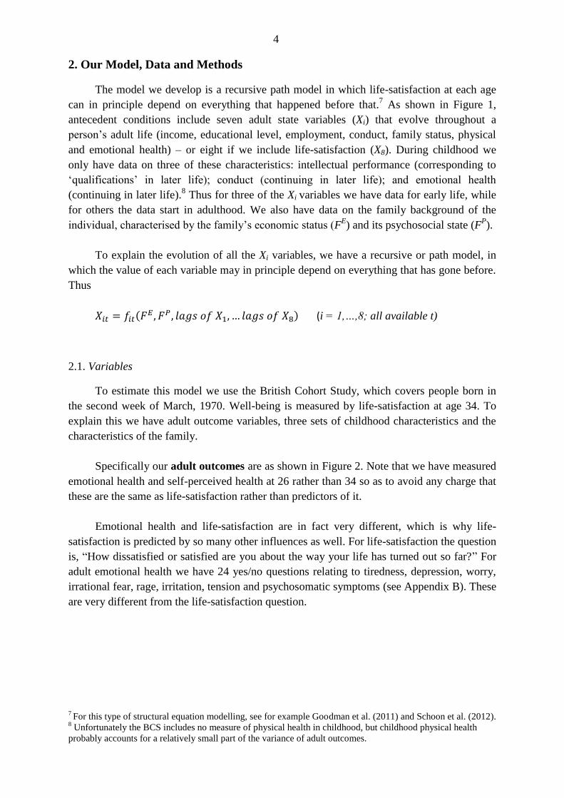
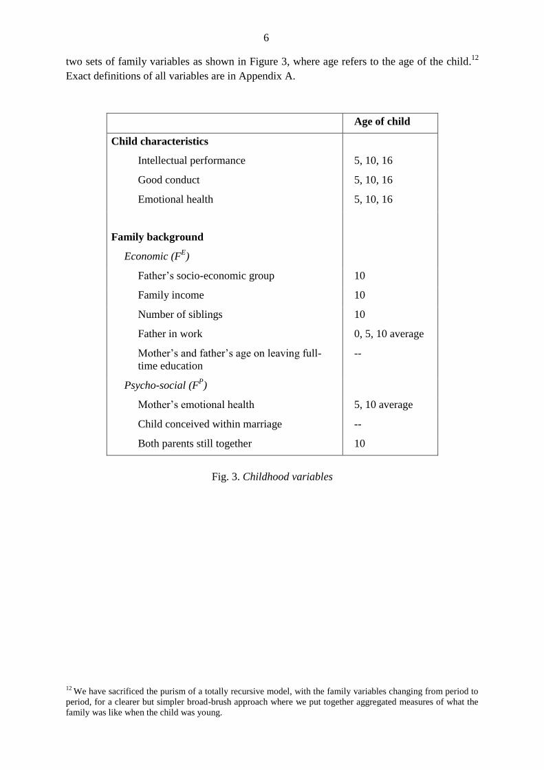
The childhood variables are shown in Figure 3. They include variables relating to the
child and to the parents (“family background”). For a child there are three main dimensions
of development – intellectual performance, social behaviour and emotional health.
Economists have traditionally focussed heavily on intellectual development, but some like
Heckman have widened the perspective to include also non-cognitive skills.9 But by this they
usually mean social behaviour or sometimes self-discipline (or grit). They do not usually
mean how the children feel – are they anxious or depressed? This is a very important
dimension of a person, and psychologists who study child development make a strong
distinction between social (externalising) development and emotional (internalising)
development. 10
This is reflected in our paper by the distinction between social and emotional
learning.
This difference between social behaviour and emotional health is conceptually
important, and the two variables are not highly correlated. Questions on social behaviour
relate to destroying things, fighting, stealing, disobedience, lying, bullying, being disliked
and unsettled and impulsive behaviour. Questions on children’s emotional health are more
internal, and relate to worry, unhappiness, sleeplessness, eating disorder, bedwetting,
fearfulness, school avoidance, tiredness, and psychosomatic pains. These are very different
dimensions of personality, with different effects.11
We have measurements on the three child variables at 5, 10 and 16. We also have
measurements on the family at different ages but for simplicity we consolidate these into the
9 See Cunha and Heckman (2008); Almlund et al. (2011) and Goodman et al. (2011). Recently Heckman has
extended his perspective to the 5 main (OCEAN) dimensions of personality. 10
On the measurement of children’s emotional health and behaviour, see Rutter et al. (2008). 11
To measure these two variables we take simple aggregates of answers to the individual questions. Clinical
psychologists usually do the same. Developmental psychologists often do also, but at other times they carry out
factor analysis to extract one or more factors from the multiple answers. The problem with factor analysis is that
it relies on the internal coherence of the answers, not on their predictive power. For prediction one could of
course enter each answer separately, but the problem then would be different relative weights in every separate
regression. For an approach using factor analysis see Richards and Hatch (2011).
6
two sets of family variables as shown in Figure 3, where age refers to the age of the child.12
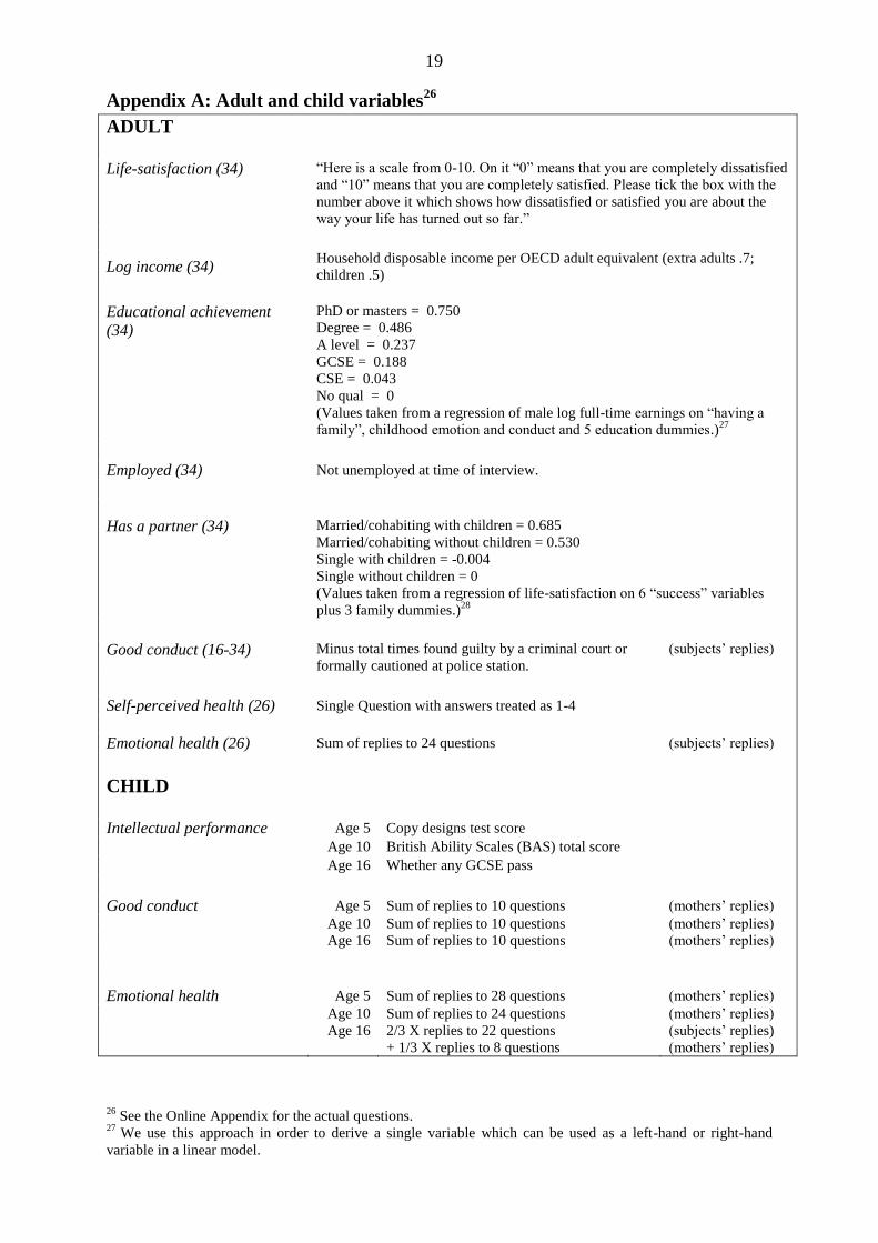
Exact definitions of all variables are in Appendix A.
Age of child
Child characteristics
Intellectual performance 5, 10, 16
Good conduct 5, 10, 16
Emotional health 5, 10, 16
Family background
Economic (FE)
Father’s socio-economic group 10
Family income 10
Number of siblings 10
Father in work 0, 5, 10 average
Mother’s and father’s age on leaving full-
time education
--
Psycho-social (FP)
Mother’s emotional health 5, 10 average
Child conceived within marriage --
Both parents still together 10
Fig. 3. Childhood variables
12
We have sacrificed the purism of a totally recursive model, with the family variables changing from period to
period, for a clearer but simpler broad-brush approach where we put together aggregated measures of what the
family was like when the child was young.
7
2.2. Method of analysis
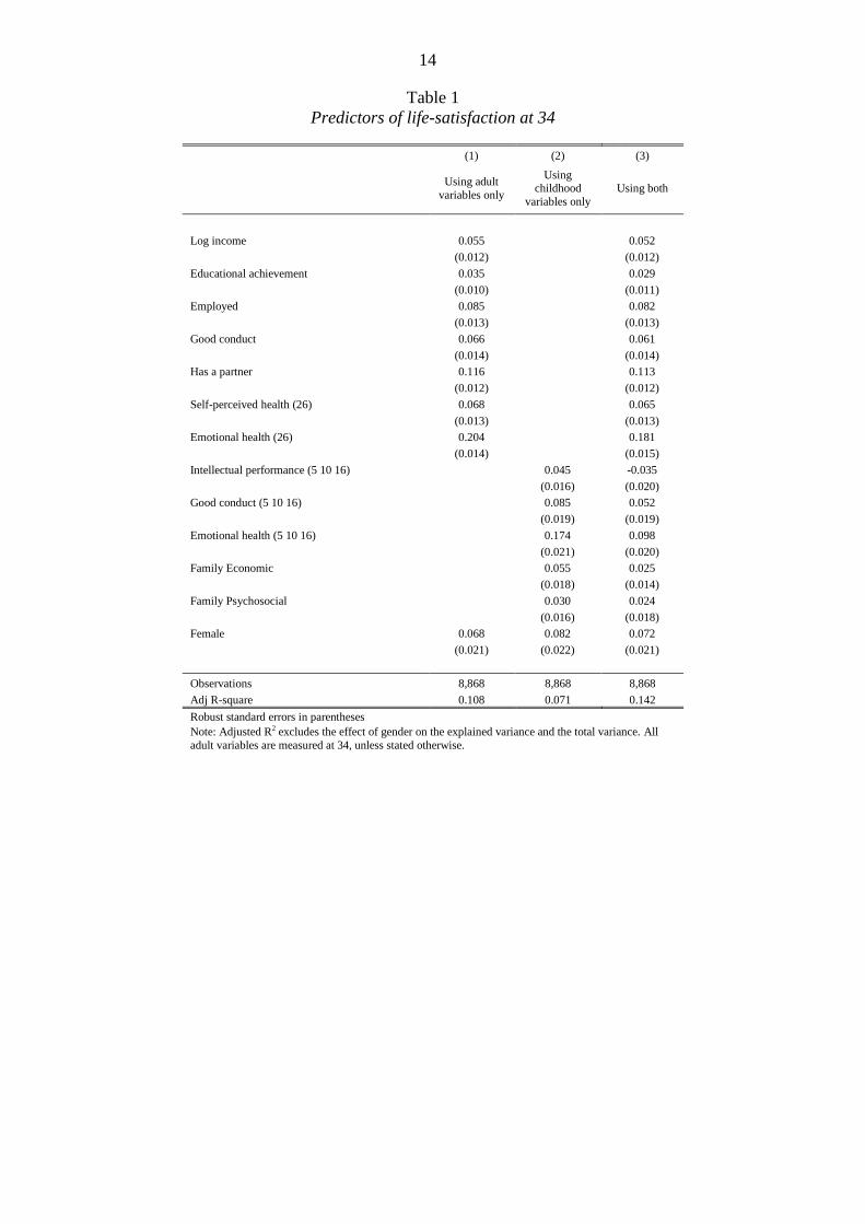
We begin in Table 1 by predicting life-satisfaction from other adult outcomes and from
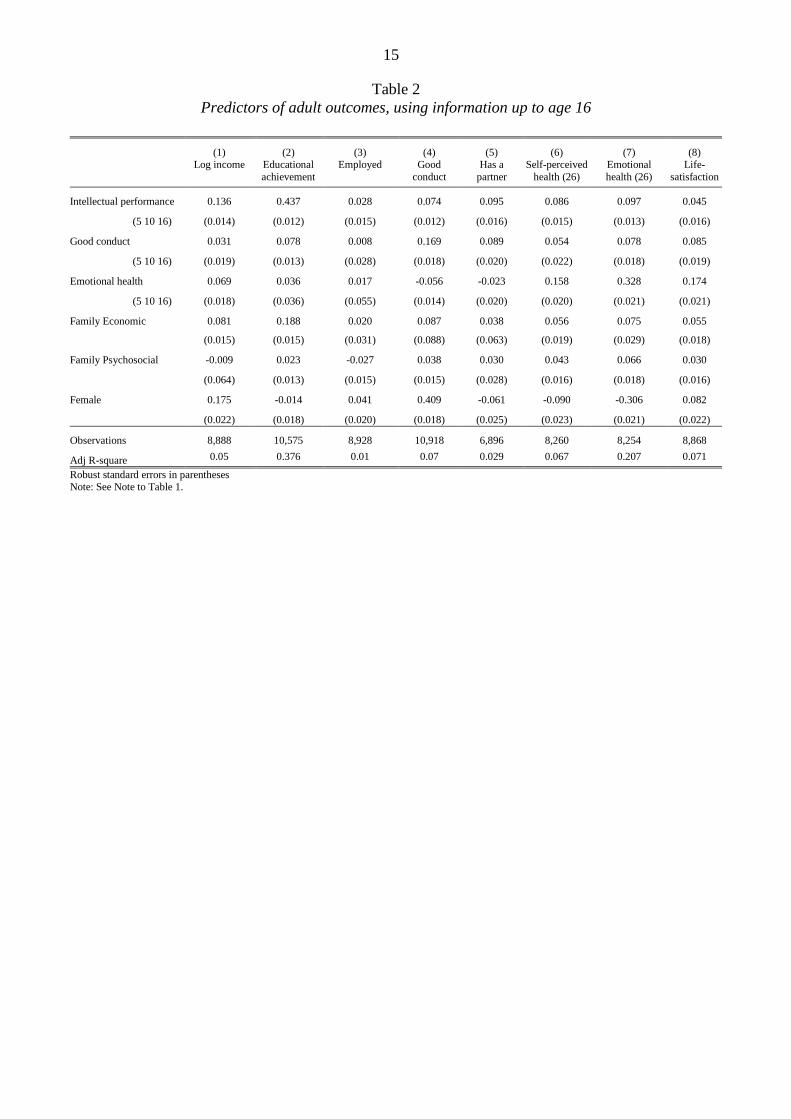
childhood variables. Then in Table 2 we examine how the other adult outcomes are
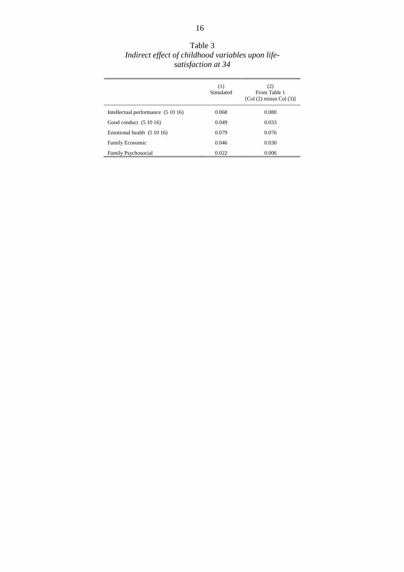
determined by childhood variables. In Table 3 we examine the issue of mediation: by what
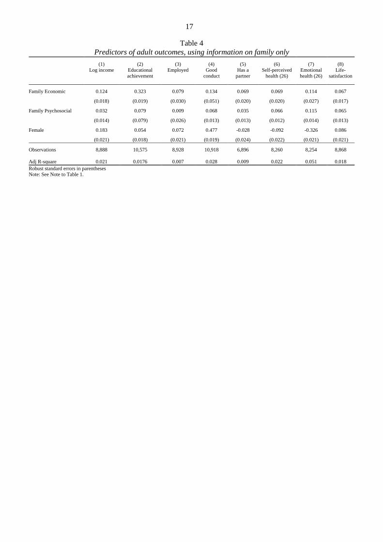
route each childhood variable affects the life-satisfaction of the adult. In Table 4 we focus on
the family as the sole predictor, and in Table 5 we examine how far adult life-satisfaction can
in fact be predicted by information available at each age. More detailed analyses are available
in an online appendix, whose contents are listed in Appendix B.
Analysis is by OLS and variables (except gender) are standardised throughout. Thus all
coefficients are standardised regression coefficients (i.e. partial correlation coefficients or β-
coefficients). The squared value of each coefficient shows how much the right-hand variable
contributes on its own to the variance of the left-hand variable (ignoring its covariance with
the other right-hand variables). It is a meaningful measure of the importance of the variable.
However, to see the wood for the trees, some simplification is helpful. Let us take an
example. Suppose we want to look at the overall effect of child conduct on adult outcomes.
We have measures of child conduct at ages 5, 10 and 16 (C5, C10, C16). In our first stage
regression for adult outcome Xi (shown in the online Appendix) we estimate the effects of
each of these conduct variables separately. This gives the following:
( ) ( )
( )
where
(
)
Thus the coefficient on the composite variable C is the sum of the separate coefficients times
the standard deviation of the composite variable, SD(C).13
This is the procedure we use
throughout to calculate the effect of composite variables.
13
(i) To compute SD(C) we use only the observations where there are no missing values on any of the variables
in the composite variable, C. For obvious reasons SD(C)<1 unless all the variables are perfectly correlated.
(ii) To obtain the standard error of the estimate of ( ) ( ) we rerun the equations replacing
C5, C10 and C16 by C. This gives an estimate of the standard error of the estimate of ( ) and we then
multiply this standard error by ( )
8
Unfortunately there are many missing values of variables. Each regression is performed
on all survey members for whom we have a non-missing value of the left-hand variable.
When there is no data on a right-hand variable, we include a variable-specific dummy to
register the fact (the so-called Missing Indicator method). We have also used as an alternative
the Multiple Imputation method and the main results are very similar – see online Appendix.
Our discussion of results is consistent with the results of both methods.
Where there are missing values, the R2 of the equation is biased downwards since all
missing values have been assigned the same (dummy) value. To simulate the true R2, we start
from the standard property of all standardised regressions. This is that if
R2
is given by
∑∑
where rij is the correlation coefficient between the two variables. So in all tables we compute
R2 using this formula, taking rij from the correlation matrix in Appendix B.
14
We can now turn to the results.
3. Results
3.1. Predictors of life-satisfaction
We begin by looking directly at the determinants of life-satisfaction. In Table 1, the
first column focuses on the proximal predictors of life-satisfaction – that is, the effect of
the individual’s other adult characteristics. Already we find a result quite different from all
previous research – the prime factor is emotional health (measured 8 years earlier). All the
other six variables also have significant effects and, as usual, education is the least important
predictor of life-satisfaction. Income explains on its own about 0.5% of the variance of life-
satisfaction – a fairly common finding.
One might of course question the validity of cross-section results like these. Clearly it
would be helpful to carry out a panel data analysis, but the BCS data do not permit this. We
adopted two strategies here, using the data for age 34 and age 26. In one analysis we
regressed the change in life-satisfaction on the change in “having a partner”, self-perceived
health and emotional health (the only 3 variables for which there are good data on changes).
The standardised coefficients for the 3 variables (comparable with those in Column 1) were
0.01, 0.09 and 0.11 – supportive of our earlier conclusions about the importance of emotional
health. In the second analysis we introduced lagged life-satisfaction on the right-hand side
and measured all 7 other variables at their age 34 level (the idea being that this would remove
14
In doing so we are attempting to use all available information to proxy the ‘true’ explanatory power of our
equations as it would be in a world without missing observations.
9
at least part of the fixed effect). The results are shown in the footnote below and are again
supportive of the conclusions from Column (1).15
What happens if, instead, we look at the distal predictors of life-satisfaction, that is
the “childhood variables” (family background and child characteristics)? The result is shown
in the second column of the table. Again emotional health emerges as the most important
variable – in childhood as in adulthood. Next comes behaviour as a child. The intellectual
development of the child is the least important of the three dimensions of child development,
when we consider life-satisfaction as the outcome of interest.
This ranking is, roughly speaking, the inverse to that of most policy-makers. In popular
discussion one encounters two main criticisms of the well-being approach (often from the
same people). One is that the concept is meaningless; the other is that, even if we accepted its
importance as a policy goal, it would make no difference to policy priorities.16
As our
evidence shows, the second point could not be more wrong.
Two other points emerge from the second column of the table. Family background
continues to matter, even after taking child characteristics into account. And women are more
satisfied with their lives, by about 8% of one standard deviation.
The next obvious question is, how does early life exert its influence on adult life-
satisfaction? If the influence were direct, one might wonder why we have so many policies
relating to adulthood – employment policy, income redistribution, health and the like. But, as
the third column shows, adult life still has an important impact on life-satisfaction even after
we have allowed for the influence of family and childhood. In Column (3), which includes
both sets of influence, the coefficients on adult characteristics are very little reduced, while
those on child characteristics are mostly reduced by about a half.
This means that roughly half the effect of childhood on adult life-satisfaction is
mediated through the effect of childhood on adult outcomes and the effect of adult outcomes
on life-satisfaction.17
The other half is a direct, unmediated effect. The exception is
intellectual performance, where the direct effect is estimated as somewhat negative but there
is a substantial mediated effect through adult outcomes.
15
Life-satisfaction at 34 = .034 log Income + .619 Educational achievement
(.010) (.009)
+ .065 Employed + .029 Good conduct + .090 Has a partner
(.011) (.012) (.011)
+ .095 Self-perceived health at 34 + .323 Emotional health at 34
(.010) (,012)
+ .258 Life-satisfaction at 26
(.013)
16
See HM Treasury (2008). 17
To think about mediation it is helpful to note the following relationships between standardised variables.
Suppose Y = aX +bZ and X = cZ. Then Y = (ac+b)Z. Since all coefficients are less than unity and (we assume)
positive, a finding that ac+b is roughly double b can only arise if a is substantially bigger than b.
10
3.2. Predictors of adult outcomes
So the next step is to examine the effect of childhood on the adult outcomes. If we look
at economic outcomes (income, unemployment and educational achievement), the most
powerful influence is the intellectual development of the child and the child’s socio-economic
background. These are of course standard findings in labour economics. However, if we turn
to the social outcomes (criminality and family formation), the pattern changes. A key thing is
how the person behaved as a child.
Finally when we come to the ‘personal’ outcomes, adult emotional health and self-
perceived health, by far the most important influence from childhood is the child’s emotional
health. This echoes our earlier finding that adult life-satisfaction depends the most heavily on
emotional health as a child.
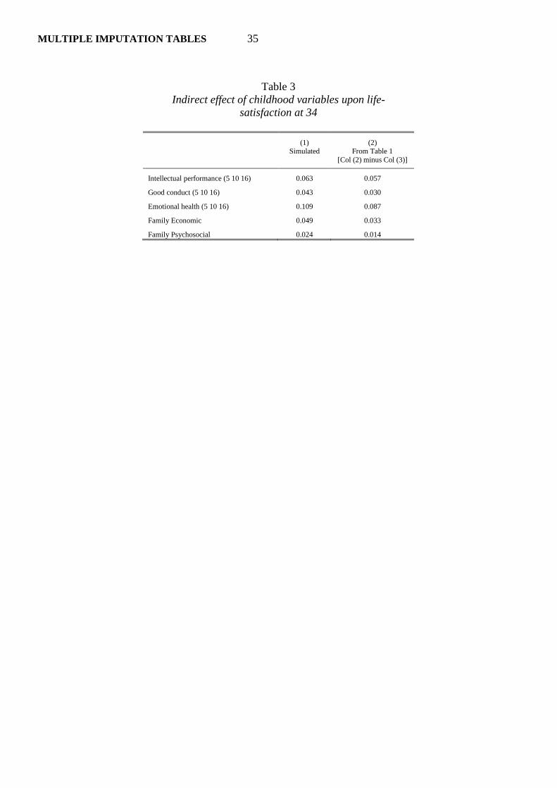
3.3. More on mediation
Now that we have charted how childhood affects adult outcomes, it is worth checking
the consistency of our earlier findings about mediation (in Table 1). In Table 3 we give the
estimated indirect effect of each childhood variable, combining the way it affects adult
outcomes (in Table 2) with the way these outcomes affect life-satisfaction (in Table 1,
Column 3). The results are given in the left hand column of Table 3. We can now compare
these ‘simulated’ indirect effects with the indirect effects implied in Table 1 (by the
difference between columns (2) and (3)). As can be seen, the estimates are close, which
confirms that we have a consistent story.
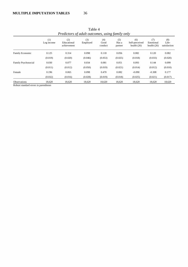
3.4. The effect of the family
As we have noted, the effect of family variables is small, once childhood variables are
taken into account. But these childhood variables are themselves affected by family
influences. So what happens if we look at the reduced form equations, where we include only
the effect (direct and indirect) of family characteristics on adult outcomes (see Table 4)?
The family of course emerges as more important, particularly as a predictor of
educational performance and income – the variables hitherto most studied by economists. But
(in so far as we can measure the family’s characteristics) family variables have a relatively
more limited impact on life-satisfaction, criminal behaviour, and family formation.
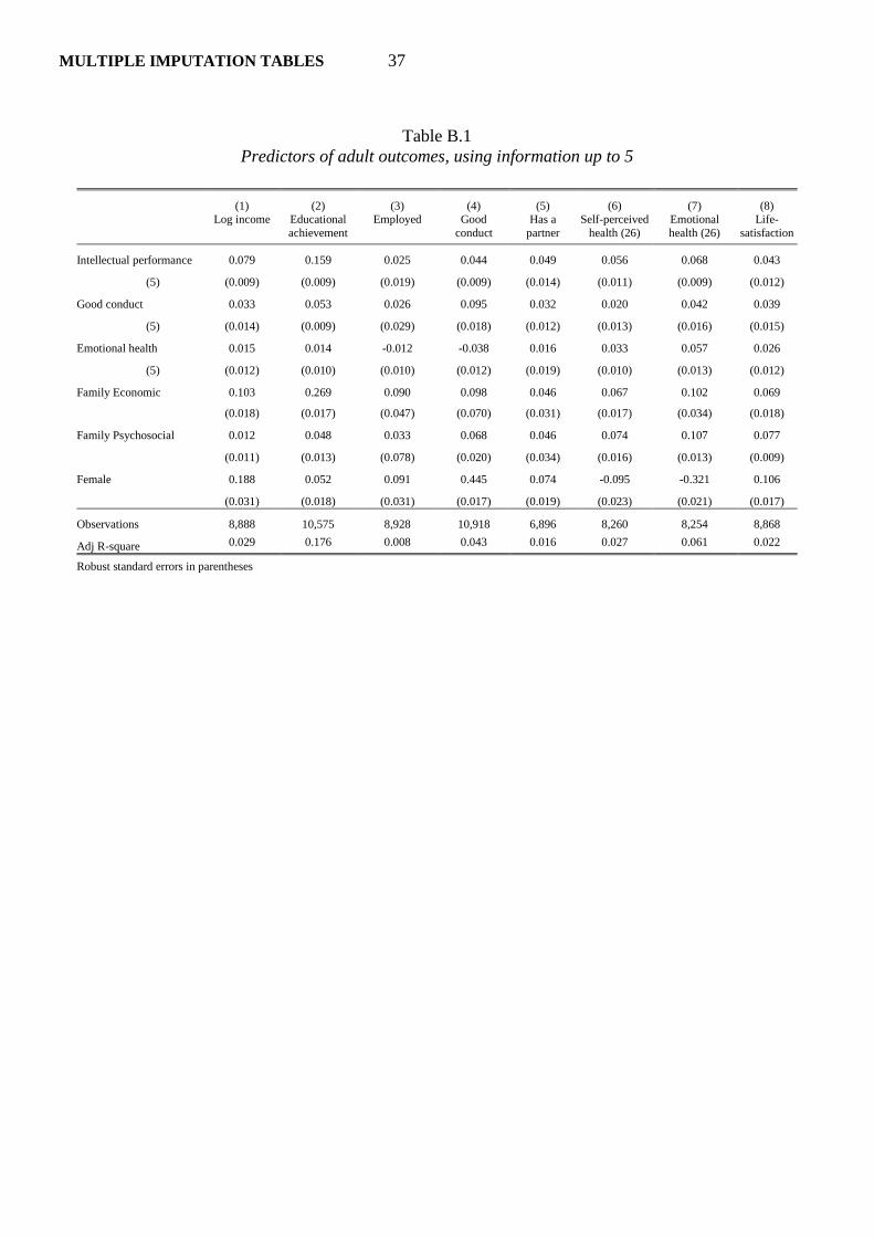
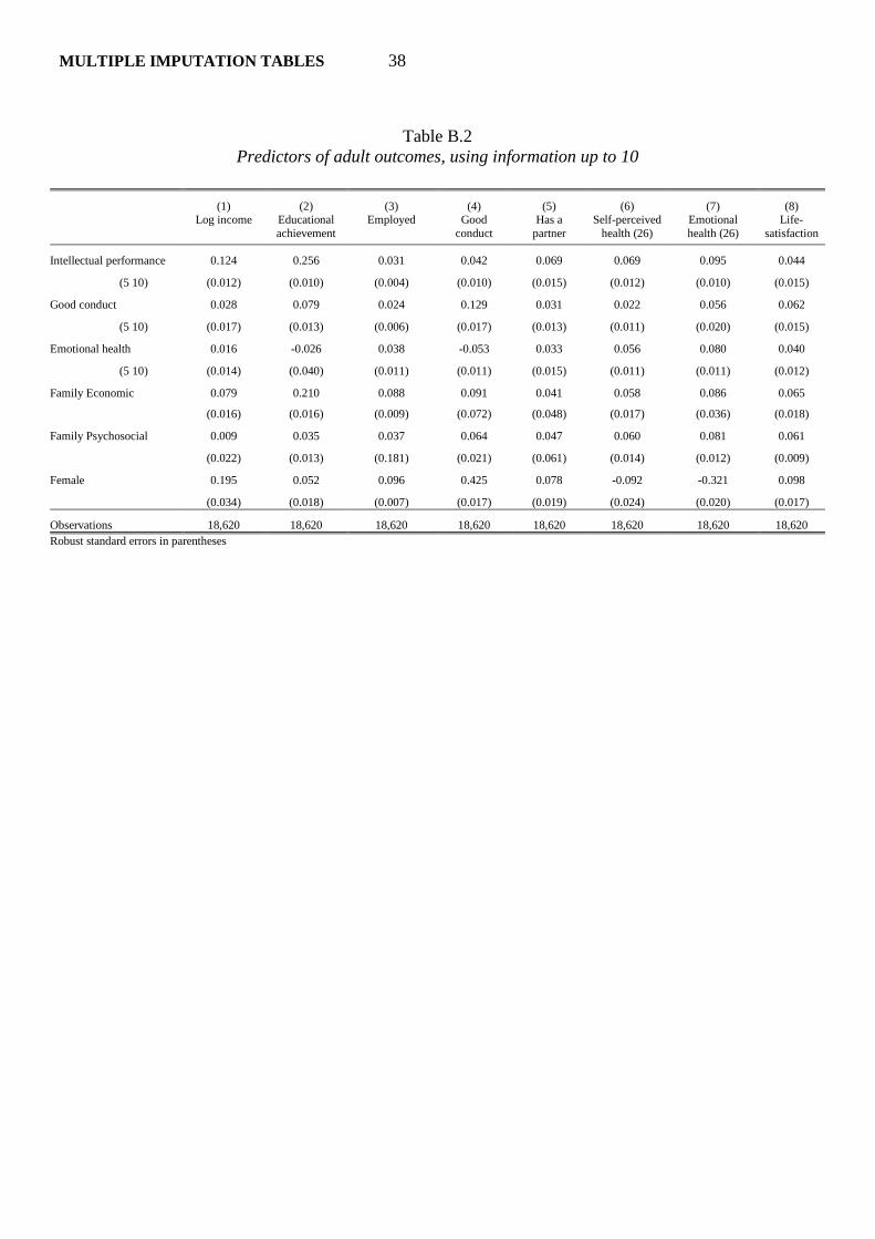
3.5. Does the child reveal the adult?
This brings us to a final question. At what stage of a person’s development does it
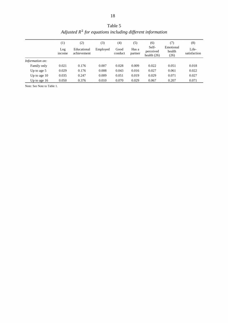
become at all possible to predict their adult outcomes? We examine this in Table 5.
It has recently become quite fashionable to argue that by age 5 key experiences (plus
genes) have largely determined a person’s outcomes as an adult. This is done by showing
large odds ratios between the adult outcomes of more and less advantaged children. But the
proper test of predictability is the R2s. These are shown in Table 5.
11
The table shows how well we can predict each adult outcome from information
available about a person at different stages of their life – birth (roughly speaking), age 5, age
10, and age 16. As Frijters, Johnston and Shields18
have pointed out, life-satisfaction is
extremely difficult to predict even at age 10 and only slightly easier at age 16. The most
predictable feature is educational achievement. But income is extremely difficult to predict,
as is life-satisfaction. Almost all outcomes are much easier to predict at age 16 than at age 5,
indicating the importance of a balance between earlier and later intervention.19
4. Use for Policy Analysis
Any future policy-maker aiming at population well-being will need to use a model of
the kind we have been discussing – including genetic controls if possible.20
A life-course
model is the product of the interaction between millions of individuals and the institutions in
which they live. It is not a law of nature. But it is the correct starting point for considering
how varying an institution or a policy would affect the citizens for better or worse. Our
existing model already suggests the need for different policy priorities. But an ideal model
would be more detailed, and refined by replication.
How would it be used? Let us assume that the policy-maker wanted to maximise the
sum of life-satisfaction of citizens of all ages.21
This would require a continuous record of
life-satisfaction at each age, plus a model of how that path was determined. And that model
would immediately suggest key areas for greater or less public policy intervention.
4.1. Effectiveness of intervention
But to know whether any particular intervention was cost-effective would ideally
require an experiment, with a long follow-up. However, such follow-ups are expensive, and
often we only know the short-run effects of an intervention. A model can therefore be
extremely useful for simulating the long-run effects of an intervention whose short-run
effects we know (but nothing more). For example, if we give parent training to a badly
behaved 5-year-old and the effect size is β. We can then go to the model and simulate all the
subsequent effects of β standard deviations change in conduct at 5.
4.2. Costs
But finding the effects is one thing; assessing the cost-effectiveness of the intervention
is another. For that we need to know not only the initial cost of the original intervention but
18
Frijters et al. (2011). 19
Clearly all findings in this paper are affected by measurement error. 20
This may become possible through greater availability of twin and adoptee studies, or better identification of
critical gene sequences in DNA (where DNA data are now routinely collected in many studies). 21
Many people believe more weight should be given to the avoidance of misery than the achievement of the
highest levels of life-satisfaction (Layard (2011), Ch.15). This would require a concave social welfare function,
based on ethical judgements. The present text ignores that complication.
12
also any impact it has on subsequent public expenditure. Some impacts will increase
subsequent public expenditure – for example, a successful education intervention may lead to
more staying on at school. Or the effects on cost may be negative – for example fewer costs
of crime and justice.
If the well-being benefits were positive and the net costs were zero or negative, that
could be decisive. And indeed much of the discussion of early intervention to date has been
of this kind.22
But public expenditure does not have to have a zero net cost to the taxpayer,
and much of it has of course a positive net cost. So many analyses of childhood interventions
will use estimates of benefits as well as net cost to get some feel for the level of cost-
effectiveness.
4.3. Cost-effectiveness
In that case how would we judge if they were cost-effective? It is best to think of the
level of public expenditure as being pre-determined, independent of the potential benefits of
current policy options. If so, the correct decision rule for evaluating an intervention is to
select a cost-effectiveness ratio (λ) such that all interventions with ratios lower than λ would
together just exhaust the available funding for public expenditure.
But all of this requires good information on cost. So future models will have to include
much more structure than the model in this paper. They will need to include all publicly-
financed activities in which the individual becomes involved (be it education, pre-school,
health-related, law and order, employment or welfare benefits). In our future work on
ALSPAC23
we plan this degree of detail.
4.4. When to intervene?
So can anything be said about where and when to intervene? These are separate issues.
The first concerns which areas of life require more intervention or less – for children is it
their emotional, behavioural or intellectual life and for adults is it income support,
employment policy, or family support?
But the second is when to intervene – earlier or later.24
If childhood well-being matters
as much as adult well-being,25
then the main issue on the benefit side is how long the effects
last. For language learning for example the answer here is clear (it lasts longer if the
intervention is earlier). But for emotional learning there is still much to be discovered. On the
cost side adult interventions generally produce immediate flow backs to public finance as
more people go out to work and earn. Child interventions can produce massive savings to
public finances but these are often quite delayed. Clearly we need interventions at all ages
and the optimum balance will remain unclear until we have better life-course models. 22
See for example, Knapp et al. (2011b). 23
Avon Longitudinal Study of Parents and Children. 24
Heckman has argued strongly in favour of early intervention. 25
As argued for example by Layard and Dunn (2009).
13
5. Conclusions
Policy-makers need models which show them the impact of all the main factors
affecting adult life-satisfaction, in a consistent framework using the same metric. We estimate
such a model using the British Cohort Study (1970).
Adult life-satisfaction is directly affected by adult circumstances and by childhood
characteristics. But, even though childhood characteristics also affect adult circumstances,
they have a limited ability to predict adult life-satisfaction.
By far the most important predictor of adult life-satisfaction is emotional health, both in
childhood and subsequently. Pro-social behaviour in childhood is the next most important
predictor. And the intellectual performance of a child is the least important predictor of life-
satisfaction as an adult. These findings have massive implications for educational policy.
Intellectual performance is of course a good predictor of the person’s educational
achievement and income. But income only explains 0.5% of the variance of adult life-
satisfaction.
Family background (economic, social and psychological) is a quite limited predictor of
most adult outcomes except educational qualifications.
14
Table 1
Predictors of life-satisfaction at 34
(1) (2) (3)
Using adult
variables only
Using childhood
variables only
Using both
Log income 0.055
0.052
(0.012)
(0.012)
Educational achievement 0.035
0.029
(0.010)
(0.011)
Employed 0.085
0.082
(0.013)
(0.013)
Good conduct 0.066
0.061
(0.014)
(0.014)
Has a partner 0.116
0.113
(0.012)
(0.012)
Self-perceived health (26) 0.068
0.065
(0.013)
(0.013)
Emotional health (26) 0.204
0.181
(0.014)
(0.015)
Intellectual performance (5 10 16)
0.045 -0.035
(0.016) (0.020)
Good conduct (5 10 16)
0.085 0.052
(0.019) (0.019)
Emotional health (5 10 16)
0.174 0.098
(0.021) (0.020)
Family Economic
0.055 0.025
(0.018) (0.014)
Family Psychosocial
0.030 0.024
(0.016) (0.018)
Female 0.068 0.082 0.072
(0.021) (0.022) (0.021)
Observations 8,868 8,868 8,868
Adj R-square 0.108 0.071 0.142
Robust standard errors in parentheses
Note: Adjusted R2 excludes the effect of gender on the explained variance and the total variance. All
adult variables are measured at 34, unless stated otherwise.
15
Table 2
Predictors of adult outcomes, using information up to age 16
(1) (2) (3) (4) (5) (6) (7) (8)
Log income Educational
achievement
Employed Good
conduct
Has a
partner
Self-perceived
health (26)
Emotional
health (26)
Life-
satisfaction
Intellectual performance 0.136 0.437 0.028 0.074 0.095 0.086 0.097 0.045
(5 10 16) (0.014) (0.012) (0.015) (0.012) (0.016) (0.015) (0.013) (0.016)
Good conduct 0.031 0.078 0.008 0.169 0.089 0.054 0.078 0.085
(5 10 16) (0.019) (0.013) (0.028) (0.018) (0.020) (0.022) (0.018) (0.019)
Emotional health 0.069 0.036 0.017 -0.056 -0.023 0.158 0.328 0.174
(5 10 16) (0.018) (0.036) (0.055) (0.014) (0.020) (0.020) (0.021) (0.021)
Family Economic 0.081 0.188 0.020 0.087 0.038 0.056 0.075 0.055
(0.015) (0.015) (0.031) (0.088) (0.063) (0.019) (0.029) (0.018)
Family Psychosocial -0.009 0.023 -0.027 0.038 0.030 0.043 0.066 0.030
(0.064) (0.013) (0.015) (0.015) (0.028) (0.016) (0.018) (0.016)
Female 0.175 -0.014 0.041 0.409 -0.061 -0.090 -0.306 0.082
(0.022) (0.018) (0.020) (0.018) (0.025) (0.023) (0.021) (0.022)
Observations 8,888 10,575 8,928 10,918 6,896 8,260 8,254 8,868
Adj R-square 0.05 0.376 0.01 0.07 0.029 0.067 0.207 0.071
Robust standard errors in parentheses Note: See Note to Table 1.
16
Table 3
Indirect effect of childhood variables upon life-
satisfaction at 34
(1) (2)
Simulated From Table 1
[Col (2) minus Col (3)]
Intellectual performance (5 10 16) 0.068 0.080
Good conduct (5 10 16) 0.049 0.033
Emotional health (5 10 16) 0.079 0.076
Family Economic 0.046 0.030
Family Psychosocial 0.022 0.006
17
Table 4
Predictors of adult outcomes, using information on family only
(1) (2) (3) (4) (5) (6) (7) (8)
Log income Educational
achievement
Employed Good
conduct
Has a
partner
Self-perceived
health (26)
Emotional
health (26)
Life-
satisfaction
Family Economic 0.124 0.323 0.079 0.134 0.069 0.069 0.114 0.067
(0.018) (0.019) (0.030) (0.051) (0.020) (0.020) (0.027) (0.017)
Family Psychosocial 0.032 0.079 0.009 0.068 0.035 0.066 0.115 0.065
(0.014) (0.079) (0.026) (0.013) (0.013) (0.012) (0.014) (0.013)
Female 0.183 0.054 0.072 0.477 -0.028 -0.092 -0.326 0.086
(0.021) (0.018) (0.021) (0.019) (0.024) (0.022) (0.021) (0.021)
Observations 8,888 10,575 8,928 10,918 6,896 8,260 8,254 8,868
Adj R-square 0.021 0.0176 0.007 0.028 0.009 0.022
0.051 0.018
Robust standard errors in parentheses Note: See Note to Table 1.
18
Table 5
Adjusted for equations including different information
(1) (2) (3) (4) (5) (6) (7) (8)
Log
income
Educational
achievement
Employed
Good
conduct
Has a
partner
Self-
perceived
health (26)
Emotional
health
(26)
Life-
satisfaction
Information on:
Family only 0.021 0.176 0.007 0.028 0.009 0.022 0.051 0.018
Up to age 5 0.029 0.176 0.008 0.043 0.016 0.027 0.061 0.022
Up to age 10 0.035 0.247 0.009 0.051 0.019 0.029 0.071 0.027
Up to age 16 0.050 0.376 0.010 0.070 0.029 0.067 0.207 0.071
Note: See Note to Table 1.
19
Appendix A: Adult and child variables26
ADULT
Life-satisfaction (34) “Here is a scale from 0-10. On it “0” means that you are completely dissatisfied
and “10” means that you are completely satisfied. Please tick the box with the
number above it which shows how dissatisfied or satisfied you are about the
way your life has turned out so far.”
Log income (34) Household disposable income per OECD adult equivalent (extra adults .7;
children .5)
Educational achievement
(34)
PhD or masters = 0.750
Degree = 0.486
A level = 0.237
GCSE = 0.188
CSE = 0.043
No qual = 0
(Values taken from a regression of male log full-time earnings on “having a
family”, childhood emotion and conduct and 5 education dummies.)27
Employed (34) Not unemployed at time of interview.
Has a partner (34) Married/cohabiting with children = 0.685
Married/cohabiting without children = 0.530
Single with children = -0.004
Single without children = 0
(Values taken from a regression of life-satisfaction on 6 “success” variables
plus 3 family dummies.)28
Good conduct (16-34) Minus total times found guilty by a criminal court or
formally cautioned at police station.
(subjects’ replies)
Self-perceived health (26) Single Question with answers treated as 1-4
Emotional health (26) Sum of replies to 24 questions (subjects’ replies)
CHILD
Intellectual performance Age 5 Copy designs test score
Age 10 British Ability Scales (BAS) total score Age 16 Whether any GCSE pass
Good conduct Age 5 Sum of replies to 10 questions (mothers’ replies)
Age 10 Sum of replies to 10 questions (mothers’ replies)
Age 16 Sum of replies to 10 questions (mothers’ replies)
Emotional health Age 5 Sum of replies to 28 questions (mothers’ replies)
Age 10 Sum of replies to 24 questions (mothers’ replies)
Age 16
2/3 X replies to 22 questions
+ 1/3 X replies to 8 questions
(subjects’ replies)
(mothers’ replies)
26
See the Online Appendix for the actual questions. 27
We use this approach in order to derive a single variable which can be used as a left-hand or right-hand
variable in a linear model.
20
References
Almlund, M., Duckworth, A.L., Heckman, J.J. and Kautz, T. (2011). 'Personality psychology
and economics', in (E.A. Hanushek, S. Machin and L. Woessmann, eds.), Handbook
of the Economics of Education, pp. 1-181, Amsterdam: Elsevier.
Boyce, C.J., Wood, A.M. and Powdthavee, N. (2013). 'Is personality fixed? Personality
changes as much as "variable" economic factors and more strongly predicts changes
to life satisfaction', Social Indicators Research, vol. 111(1), pp. 287-305.
Campbell, A., Converse, P.E. and Rodgers, W.L. (1976). The Quality of American life:
Perceptions, evaluations and satisfactions, New York: Russell Sage Foundation.
Clark, A.E. and Oswald, A.J. (1994). 'Unhappiness and unemployment', Economic Journal,
vol. 104(424), pp. 648-659.
Cunha, F. and Heckman, J.J. (2008). 'Formulating, identifying and estimating the technology
of cognitive and noncognitive skill formation', Journal of Human Resources, vol. 43,
pp. 738-782.
Cunha, F., Heckman, J.J. and Schennach, S.M. (2010). 'Estimating the Technology of
Cognitive and Noncognitive Skill Formation', Econometrica, vol. 78(3), pp. 883-931.
De Neve, J.-E., Fowler, J.H., Christakis, N.A. and Frey, B.S. (2012). 'Genes, Economics, and
Happiness', Journal of Neuroscience, Psychology, and Economics, vol. 5(4), pp. 193-
211.
Frey, B.S. and Stutzer, A. (2002). Happiness and Economics: How the economy and
institutions affect well-being, Princeton and Oxford: Princeton University Press.
Frijters, P., Johnston, D.W. and Shields, M.A. (2011) 'Destined for (Un)Happiness: Does
Childhood Predict Adult Life Satisfaction?', IZA Discussion Paper Series No 5819.
Furstenberg, F.F. and Kiernan, K.E. (2001). 'Delayed parental divorce: How much do
children benefit?', Journal of Marriage and the Family, vol. 63, pp. 446-457.
Goodman, A., Joyce, R. and Smith, J.P. (2011). 'The long shadow cast by childhood physical
and mental problems on adult life', PNAS, vol. 108(15), pp. 6032-6037.
Helliwell, J.F. (2003). 'How's life? Combining individual and national variables to explain
subjective well-being', Economic Modelling, vol. 20, pp. 331-360.
HM Treasury. (2008). Developments in the economics of well-being. Treasury Economic
Working Paper 4. (J. Lepper and S. McAndrew). London: HM Treasury.
Kahneman, D., Diener, E. and Schwarz, N., Eds. (1999). Well-Being: The Foundations of
Hedonic Psychology. New York: Russell Sage Foundation.
Knapp, M., King, D., Healey, A. and Thomas, C. (2011a). 'Economic outcomes in adulthood
and their associations with antisocial conduct, attention deficit and anxiety problems
in childhood', Journal of Mental Health Policy and Economics, vol. 14(3), pp. 137-
147.
Knapp, M., McDaid, D. and Parsonage, M., Eds. (2011b). Mental health promotion and
mental illness prevention: The economic case. London: Department of Health.
Layard, R. (2011). Happiness: Lessons from a new science (Second edition), London:
Penguin.
Layard, R., Clark, A.E. and Senik, C. (2012). 'The Causes of Happiness and Misery', in (J.
Helliwell, R. Layard and J. Sachs, eds.), World Happiness Report, pp. 58-89: The
Earth Institute, Columbia University, CIFAR, and CEP.
Layard, R. and Dunn, J. (2009). A Good Childhood - Searching for values in a competitive
age, London: Penguin.
OECD. (2013). OECD Guidelines on Measuring Subjective Well-being. Paris: OECD
Publishing.
21
Richards, M. and Hatch, S.L. (2011). 'A life course approach to the development of mental
skills', The Journals of Gerontology, Series B: Psychological Sciences and Social
Sciences, vol. 66B(S1), pp. i26-i35.
Richards, M. and Huppert, F.A. (2011). 'Do positive children become positive adults?
Evidence from a longitudinal birth cohort study', The Journal of Positive Psychology,
vol. 6(1), pp. 75-87.
Rutter, M., Bishop, D., Pine, D.S., Scott, S., Stevenson, J.S., Taylor, E.A. and Thapar, A.,
Eds. (2008). Rutter's Child and Adolescent Psychiatry (Fifth edition). Oxford: Wiley-
Blackwell.
Schoon, I., Barnes, M., Brown, V., Parsons, S., Ross, A. and Vignoles, A. (2012).
Intergenerational transmission of worklessness: Evidence from the Millennium
Cohort and the Longitudinal Study of Young People in England. Research Report
DFE-RR234. London: Department for Education.
ONLINE ANNEX
Appendix B
OLS Tables
Table B.1. Predictors of adult outcomes: using information up to age 5.
Table B.2. Predictors of adult outcomes: using information up to age 10.
Table B.3. Predictors of outcomes at age 5: using information on family only.
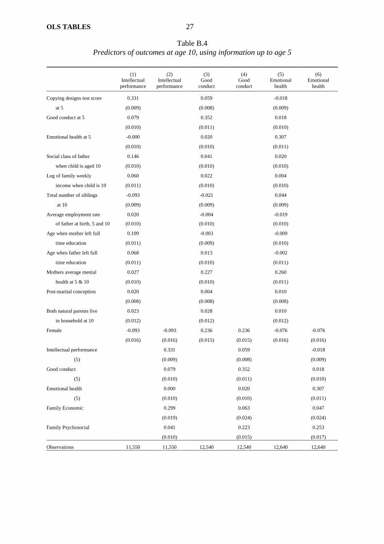
Table B.4. Predictors of outcomes at age 10: using information up to age 5.
Table B.5. Predictors of outcomes at age 16: using information up to age 10.
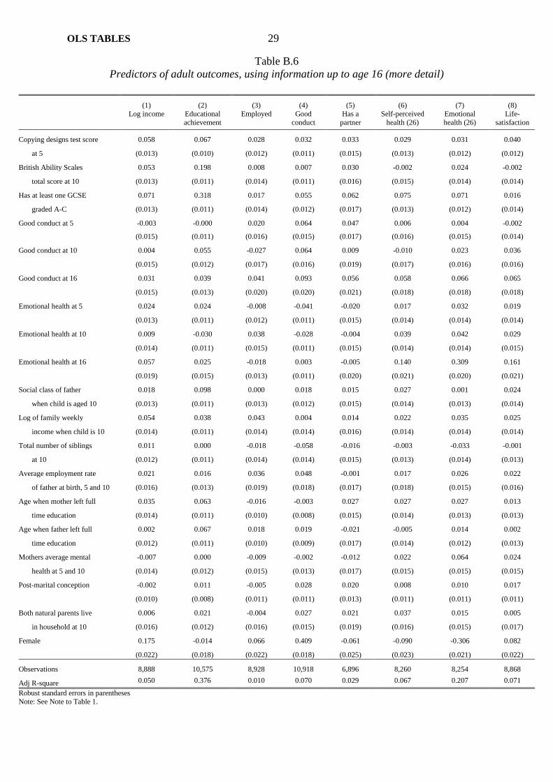
Table B.6. Predictors of adult outcomes: using information up to age 16 (more detail)
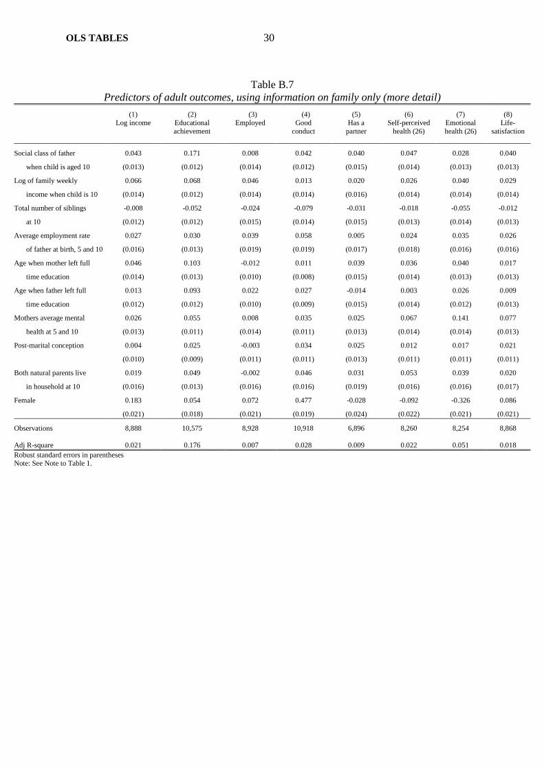
Table B.7. Predictors of adult outcomes: using information on family only (more detail)
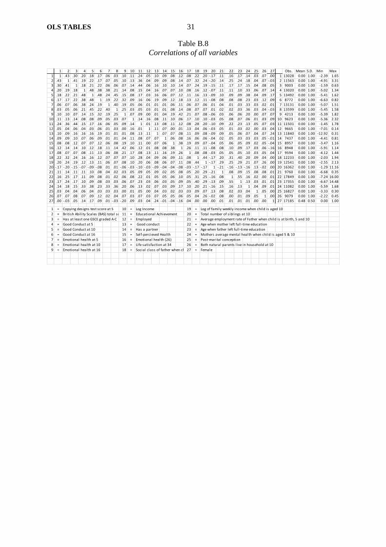
Table B.8. Correlations of all variables.
Multiple Imputation tables
Text Tables (as in text)
Appendix tables (as above)
Questionnaires

23
OLS TABLES
OLS TABLES 24
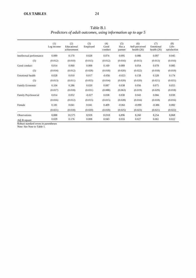
Table B.1
Predictors of adult outcomes, using information up to age 5
(1) (2) (3) (4) (5) (6) (7) (8)
Log income Educational achievement
Employed Good conduct
Has a partner
Self-perceived health (26)
Emotional health (26)
Life-satisfaction
Intellectual performance 0.089 0.170 0.028 0.074 0.095 0.086 0.097 0.045
(5) (0.012) (0.010) (0.015) (0.012) (0.016) (0.015) (0.013) (0.016)
Good conduct 0.014 0.060 0.008 0.169 0.089 0.054 0.078 0.085
(5) (0.014) (0.012) (0.028) (0.018) (0.020) (0.022) (0.018) (0.019)
Emotional health 0.028 0.010 0.017 -0.056 -0.023 0.158 0.328 0.174
(5) (0.013) (0.011) (0.055) (0.014) (0.020) (0.020) (0.021) (0.021)
Family Economic 0.104 0.286 0.020 0.087 0.038 0.056 0.075 0.055
(0.017) (0.018) (0.031) (0.088) (0.063) (0.019) (0.029) (0.018)
Family Psychosocial 0.014 0.052 -0.027 0.038 0.030 0.043 0.066 0.030
(0.016) (0.012) (0.015) (0.015) (0.028) (0.016) (0.018) (0.016)
Female 0.181 0.041 0.041 0.409 -0.061 -0.090 -0.306 0.082
(0.021) (0.018) (0.020) (0.018) (0.025) (0.023) (0.021) (0.022)
Observations 8,888 10,575 8,928 10,918 6,896 8,260 8,254 8,868
Adj R-square 0.029 0.176 0.008 0.043 0.016 0.027 0.061 0.022
Robust standard errors in parentheses Note: See Note to Table 1.
OLS TABLES 25
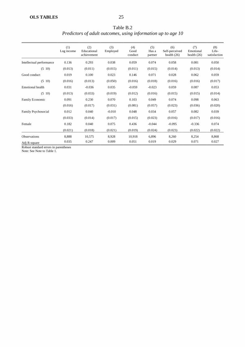
Table B.2
Predictors of adult outcomes, using information up to age 10
(1) (2) (3) (4) (5) (6) (7) (8)
Log income Educational
achievement
Employed Good
conduct
Has a
partner
Self-perceived
health (26)
Emotional
health (26)
Life-
satisfaction
Intellectual performance 0.136 0.293 0.038 0.059 0.074 0.058 0.081 0.050
(5 10) (0.013) (0.011) (0.015) (0.011) (0.015) (0.014) (0.013) (0.014)
Good conduct 0.019 0.100 0.023 0.146 0.071 0.028 0.062 0.059
(5 10) (0.016) (0.013) (0.050) (0.016) (0.018) (0.016) (0.016) (0.017)
Emotional health 0.031 -0.036 0.035 -0.059 -0.023 0.059 0.087 0.053
(5 10) (0.013) (0.033) (0.019) (0.012) (0.016) (0.015) (0.015) (0.014)
Family Economic 0.091 0.230 0.070 0.103 0.049 0.074 0.098 0.063
(0.016) (0.017) (0.031) (0.081) (0.057) (0.023) (0.036) (0.020)
Family Psychosocial 0.012 0.040 -0.010 0.048 0.034 0.057 0.082 0.039
(0.033) (0.014) (0.017) (0.015) (0.023) (0.016) (0.017) (0.016)
Female 0.182 0.040 0.075 0.436 -0.044 -0.095 -0.336 0.074
(0.021) (0.018) (0.021) (0.019) (0.024) (0.023) (0.022) (0.022)
Observations 8,888 10,575 8,928 10,918 6,896 8,260 8,254 8,868
Adj R-square 0.035 0.247 0.009 0.051 0.019 0.029 0.071 0.027
Robust standard errors in parentheses Note: See Note to Table 1.
OLS TABLES 26
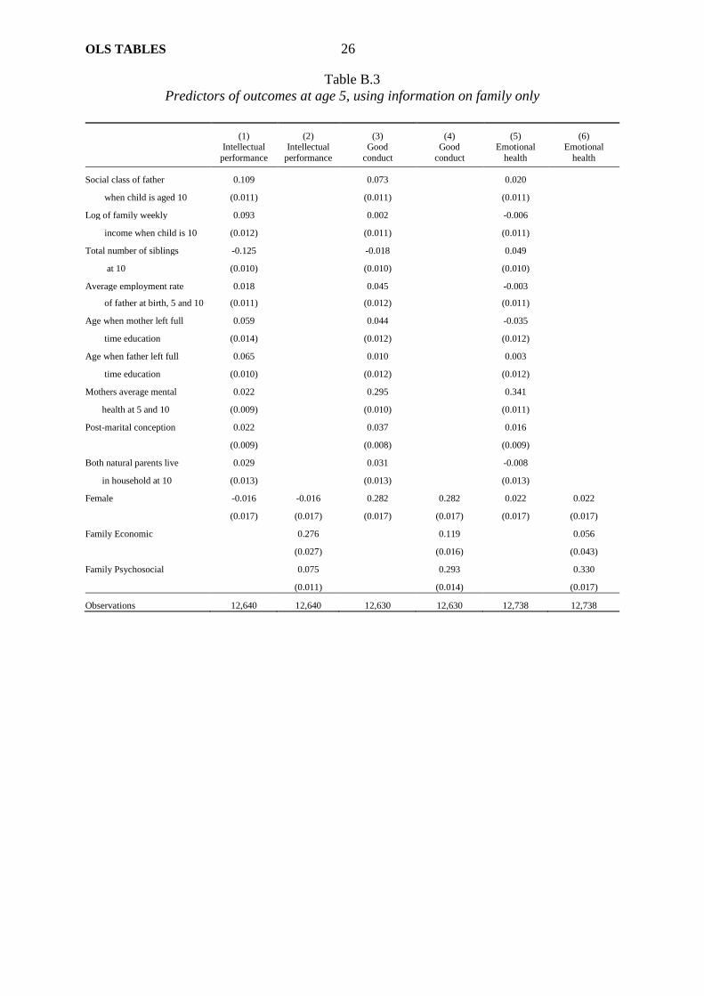
Table B.3
Predictors of outcomes at age 5, using information on family only
(1) (2) (3) (4) (5) (6)
Intellectual
performance
Intellectual
performance
Good
conduct
Good
conduct
Emotional
health
Emotional
health
Social class of father 0.109
0.073
0.020
when child is aged 10 (0.011)
(0.011)
(0.011)
Log of family weekly 0.093
0.002
-0.006
income when child is 10 (0.012)
(0.011)
(0.011)
Total number of siblings -0.125
-0.018
0.049
at 10 (0.010)
(0.010)
(0.010)
Average employment rate 0.018
0.045
-0.003
of father at birth, 5 and 10 (0.011)
(0.012)
(0.011)
Age when mother left full 0.059
0.044
-0.035
time education (0.014)
(0.012)
(0.012)
Age when father left full 0.065
0.010
0.003
time education (0.010)
(0.012)
(0.012)
Mothers average mental 0.022 0.295 0.341
health at 5 and 10 (0.009) (0.010) (0.011)
Post-marital conception 0.022 0.037 0.016
(0.009) (0.008) (0.009)
Both natural parents live 0.029 0.031 -0.008
in household at 10 (0.013) (0.013) (0.013)
Female -0.016 -0.016 0.282 0.282 0.022 0.022
(0.017) (0.017) (0.017) (0.017) (0.017) (0.017)
Family Economic 0.276 0.119 0.056
(0.027) (0.016) (0.043)
Family Psychosocial 0.075 0.293 0.330
(0.011) (0.014) (0.017)
Observations 12,640 12,640 12,630 12,630 12,738 12,738
OLS TABLES 27
Table B.4
Predictors of outcomes at age 10, using information up to age 5
(1) (2) (3) (4) (5) (6)
Intellectual
performance
Intellectual
performance
Good
conduct
Good
conduct
Emotional
health
Emotional
health
Copying designs test score 0.331 0.059 -0.018
at 5 (0.009) (0.008) (0.009)
Good conduct at 5 0.079 0.352 0.018
(0.010) (0.011) (0.010)
Emotional health at 5 -0.000 0.020 0.307
(0.010) (0.010) (0.011)
Social class of father 0.146
0.041
0.020
when child is aged 10 (0.010)
(0.010)
(0.010)
Log of family weekly 0.060
0.022
0.004
income when child is 10 (0.011)
(0.010)
(0.010)
Total number of siblings -0.093
-0.021
0.044
at 10 (0.009)
(0.009)
(0.009)
Average employment rate 0.020
-0.004
-0.019
of father at birth, 5 and 10 (0.010)
(0.010)
(0.010)
Age when mother left full 0.109
-0.003
-0.009
time education (0.011)
(0.009)
(0.010)
Age when father left full 0.068
0.013
-0.002
time education (0.011)
(0.010)
(0.011)
Mothers average mental 0.027 0.227 0.260
health at 5 & 10 (0.010) (0.010) (0.011)
Post-marital conception 0.020 0.004 0.010
(0.008) (0.008) (0.008)
Both natural parents live 0.023 0.028 0.010
in household at 10 (0.012) (0.012) (0.012)
Female -0.093 -0.093 0.236 0.236 -0.076 -0.076
(0.016) (0.016) (0.015) (0.015) (0.016) (0.016)
Intellectual performance 0.331 0.059 -0.018
(5) (0.009) (0.008) (0.009)
Good conduct 0.079 0.352 0.018
(5) (0.010) (0.011) (0.010)
Emotional health 0.000 0.020 0.307
(5) (0.010) (0.010) (0.011)
Family Economic 0.299 0.063 0.047
(0.019) (0.024) (0.024)
Family Psychosocial 0.041 0.223 0.253
(0.010) (0.015) (0.017)
Observations 11,550 11,550 12,540 12,540 12,640 12,640
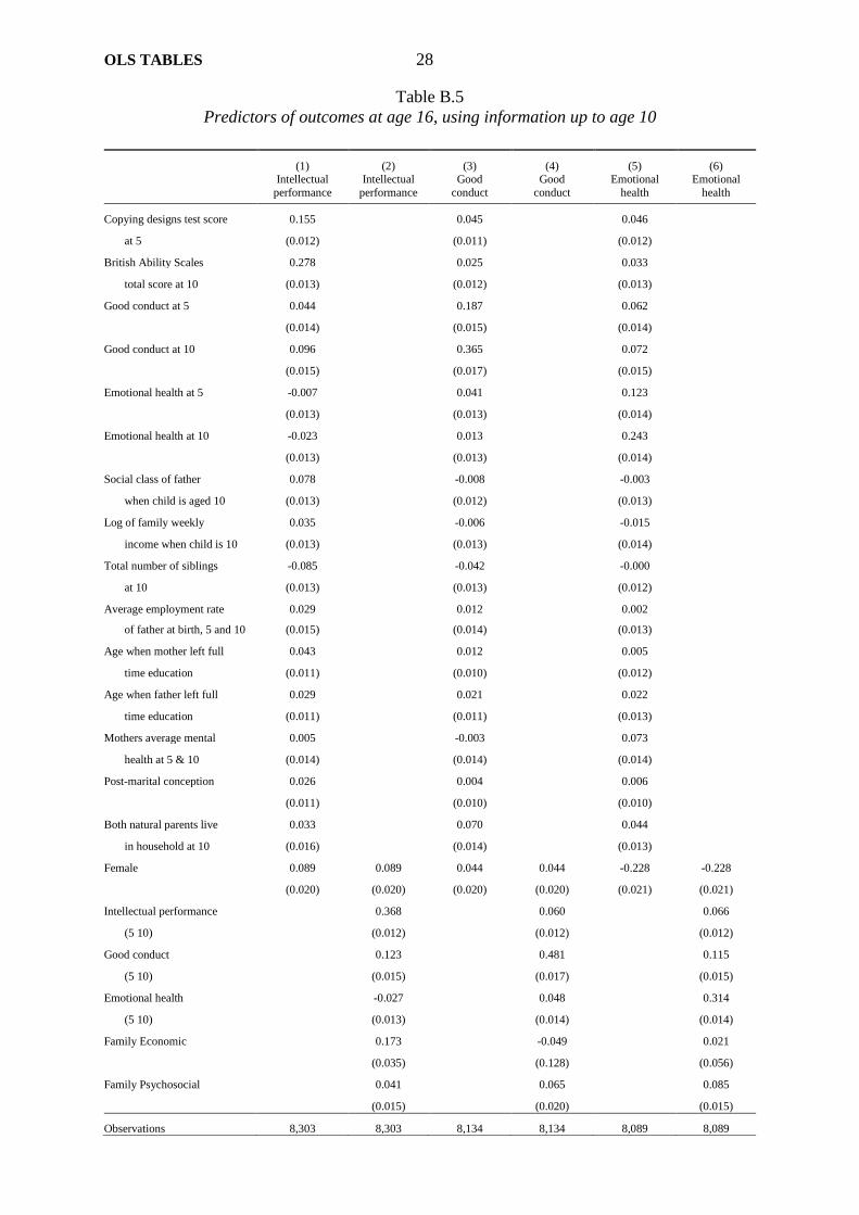
OLS TABLES 28
Table B.5
Predictors of outcomes at age 16, using information up to age 10
(1) (2) (3) (4) (5) (6)
Intellectual
performance
Intellectual
performance
Good
conduct
Good
conduct
Emotional
health
Emotional
health
Copying designs test score 0.155 0.045 0.046
at 5 (0.012) (0.011) (0.012)
British Ability Scales 0.278 0.025 0.033
total score at 10 (0.013) (0.012) (0.013)
Good conduct at 5 0.044 0.187 0.062
(0.014) (0.015) (0.014)
Good conduct at 10 0.096 0.365 0.072
(0.015) (0.017) (0.015)
Emotional health at 5 -0.007 0.041 0.123
(0.013) (0.013) (0.014)
Emotional health at 10 -0.023 0.013 0.243
(0.013) (0.013) (0.014)
Social class of father 0.078
-0.008
-0.003
when child is aged 10 (0.013)
(0.012)
(0.013)
Log of family weekly 0.035
-0.006
-0.015
income when child is 10 (0.013)
(0.013)
(0.014)
Total number of siblings -0.085
-0.042
-0.000
at 10 (0.013)
(0.013)
(0.012)
Average employment rate 0.029
0.012
0.002
of father at birth, 5 and 10 (0.015)
(0.014)
(0.013)
Age when mother left full 0.043
0.012
0.005
time education (0.011)
(0.010)
(0.012)
Age when father left full 0.029
0.021
0.022
time education (0.011)
(0.011)
(0.013)
Mothers average mental 0.005 -0.003 0.073
health at 5 & 10 (0.014) (0.014) (0.014)
Post-marital conception 0.026 0.004 0.006
(0.011) (0.010) (0.010)
Both natural parents live 0.033 0.070 0.044
in household at 10 (0.016) (0.014) (0.013)
Female 0.089 0.089 0.044 0.044 -0.228 -0.228
(0.020) (0.020) (0.020) (0.020) (0.021) (0.021)
Intellectual performance 0.368 0.060 0.066
(5 10) (0.012) (0.012) (0.012)
Good conduct 0.123 0.481 0.115
(5 10) (0.015) (0.017) (0.015)
Emotional health -0.027 0.048 0.314
(5 10) (0.013) (0.014) (0.014)
Family Economic 0.173 -0.049 0.021
(0.035) (0.128) (0.056)
Family Psychosocial 0.041 0.065 0.085
(0.015) (0.020) (0.015)
Observations 8,303 8,303 8,134 8,134 8,089 8,089
OLS TABLES 29
Table B.6
Predictors of adult outcomes, using information up to age 16 (more detail)
(1) (2) (3) (4) (5) (6) (7) (8)
Log income Educational
achievement
Employed Good
conduct
Has a
partner
Self-perceived
health (26)
Emotional
health (26)
Life-
satisfaction
Copying designs test score 0.058 0.067 0.028 0.032 0.033 0.029 0.031 0.040
at 5 (0.013) (0.010) (0.012) (0.011) (0.015) (0.013) (0.012) (0.012)
British Ability Scales 0.053 0.198 0.008 0.007 0.030 -0.002 0.024 -0.002
total score at 10 (0.013) (0.011) (0.014) (0.011) (0.016) (0.015) (0.014) (0.014)
Has at least one GCSE 0.071 0.318 0.017 0.055 0.062 0.075 0.071 0.016
graded A-C (0.013) (0.011) (0.014) (0.012) (0.017) (0.013) (0.012) (0.014)
Good conduct at 5 -0.003 -0.000 0.020 0.064 0.047 0.006 0.004 -0.002
(0.015) (0.011) (0.016) (0.015) (0.017) (0.016) (0.015) (0.014)
Good conduct at 10 0.004 0.055 -0.027 0.064 0.009 -0.010 0.023 0.036
(0.015) (0.012) (0.017) (0.016) (0.019) (0.017) (0.016) (0.016)
Good conduct at 16 0.031 0.039 0.041 0.093 0.056 0.058 0.066 0.065
(0.015) (0.013) (0.020) (0.020) (0.021) (0.018) (0.018) (0.018)
Emotional health at 5 0.024 0.024 -0.008 -0.041 -0.020 0.017 0.032 0.019
(0.013) (0.011) (0.012) (0.011) (0.015) (0.014) (0.014) (0.014)
Emotional health at 10 0.009 -0.030 0.038 -0.028 -0.004 0.039 0.042 0.029
(0.014) (0.011) (0.015) (0.011) (0.015) (0.014) (0.014) (0.015)
Emotional health at 16 0.057 0.025 -0.018 0.003 -0.005 0.140 0.309 0.161
(0.019) (0.015) (0.013) (0.011) (0.020) (0.021) (0.020) (0.021)
Social class of father 0.018 0.098 0.000 0.018 0.015 0.027 0.001 0.024
when child is aged 10 (0.013) (0.011) (0.013) (0.012) (0.015) (0.014) (0.013) (0.014)
Log of family weekly 0.054 0.038 0.043 0.004 0.014 0.022 0.035 0.025
income when child is 10 (0.014) (0.011) (0.014) (0.014) (0.016) (0.014) (0.014) (0.014)
Total number of siblings 0.011 0.000 -0.018 -0.058 -0.016 -0.003 -0.033 -0.001
at 10 (0.012) (0.011) (0.014) (0.014) (0.015) (0.013) (0.014) (0.013)
Average employment rate 0.021 0.016 0.036 0.048 -0.001 0.017 0.026 0.022
of father at birth, 5 and 10 (0.016) (0.013) (0.019) (0.018) (0.017) (0.018) (0.015) (0.016)
Age when mother left full 0.035 0.063 -0.016 -0.003 0.027 0.027 0.027 0.013
time education (0.014) (0.011) (0.010) (0.008) (0.015) (0.014) (0.013) (0.013)
Age when father left full 0.002 0.067 0.018 0.019 -0.021 -0.005 0.014 0.002
time education (0.012) (0.011) (0.010) (0.009) (0.017) (0.014) (0.012) (0.013)
Mothers average mental -0.007 0.000 -0.009 -0.002 -0.012 0.022 0.064 0.024
health at 5 and 10 (0.014) (0.012) (0.015) (0.013) (0.017) (0.015) (0.015) (0.015)
Post-marital conception -0.002 0.011 -0.005 0.028 0.020 0.008 0.010 0.017
(0.010) (0.008) (0.011) (0.011) (0.013) (0.011) (0.011) (0.011)
Both natural parents live 0.006 0.021 -0.004 0.027 0.021 0.037 0.015 0.005
in household at 10 (0.016) (0.012) (0.016) (0.015) (0.019) (0.016) (0.015) (0.017)
Female 0.175 -0.014 0.066 0.409 -0.061 -0.090 -0.306 0.082
(0.022) (0.018) (0.022) (0.018) (0.025) (0.023) (0.021) (0.022)
Observations 8,888 10,575 8,928 10,918 6,896 8,260 8,254 8,868
Adj R-square 0.050 0.376 0.010 0.070 0.029 0.067 0.207 0.071
Robust standard errors in parentheses
Note: See Note to Table 1.
OLS TABLES 30
Table B.7
Predictors of adult outcomes, using information on family only (more detail)
(1) (2) (3) (4) (5) (6) (7) (8)
Log income Educational
achievement
Employed Good
conduct
Has a
partner
Self-perceived
health (26)
Emotional
health (26)
Life-
satisfaction
Social class of father 0.043 0.171 0.008 0.042 0.040 0.047 0.028 0.040
when child is aged 10 (0.013) (0.012) (0.014) (0.012) (0.015) (0.014) (0.013) (0.013)
Log of family weekly 0.066 0.068 0.046 0.013 0.020 0.026 0.040 0.029
income when child is 10 (0.014) (0.012) (0.014) (0.014) (0.016) (0.014) (0.014) (0.014)
Total number of siblings -0.008 -0.052 -0.024 -0.079 -0.031 -0.018 -0.055 -0.012
at 10 (0.012) (0.012) (0.015) (0.014) (0.015) (0.013) (0.014) (0.013)
Average employment rate 0.027 0.030 0.039 0.058 0.005 0.024 0.035 0.026
of father at birth, 5 and 10 (0.016) (0.013) (0.019) (0.019) (0.017) (0.018) (0.016) (0.016)
Age when mother left full 0.046 0.103 -0.012 0.011 0.039 0.036 0.040 0.017
time education (0.014) (0.013) (0.010) (0.008) (0.015) (0.014) (0.013) (0.013)
Age when father left full 0.013 0.093 0.022 0.027 -0.014 0.003 0.026 0.009
time education (0.012) (0.012) (0.010) (0.009) (0.015) (0.014) (0.012) (0.013)
Mothers average mental 0.026 0.055 0.008 0.035 0.025 0.067 0.141 0.077
health at 5 and 10 (0.013) (0.011) (0.014) (0.011) (0.013) (0.014) (0.014) (0.013)
Post-marital conception 0.004 0.025 -0.003 0.034 0.025 0.012 0.017 0.021
(0.010) (0.009) (0.011) (0.011) (0.013) (0.011) (0.011) (0.011)
Both natural parents live 0.019 0.049 -0.002 0.046 0.031 0.053 0.039 0.020
in household at 10 (0.016) (0.013) (0.016) (0.016) (0.019) (0.016) (0.016) (0.017)
Female 0.183 0.054 0.072 0.477 -0.028 -0.092 -0.326 0.086
(0.021) (0.018) (0.021) (0.019) (0.024) (0.022) (0.021) (0.021)
Observations 8,888 10,575 8,928 10,918 6,896 8,260 8,254 8,868
Adj R-square 0.021 0.176 0.007 0.028 0.009 0.022
0.051 0.018
Robust standard errors in parentheses Note: See Note to Table 1.
OLS TABLES 31
Table B.8
Correlations of all variables
1 2 3 4 5 6 7 8 9 10 11 12 13 14 15 16 17 18 19 20 21 22 23 24 25 26 27 Obs. Mean S.D. Min Max1 1 .43 .30 .20 .18 .17 .06 .03 .10 .11 .24 .05 .10 .09 .08 .12 .08 .22 .20 -.17 .11 .16 .17 .14 .03 .07 .00 1 13028 0.00 1.00 -2.39 1.652 .43 1 .41 .19 .22 .17 .07 .05 .10 .13 .36 .04 .09 .09 .08 .14 .07 .32 .24 -.20 .14 .25 .24 .18 .04 .07 -.03 2 11563 0.00 1.00 -4.91 3.313 .30 .41 1 .18 .21 .22 .06 .06 .07 .14 .44 .06 .16 .10 .10 .14 .07 .24 .19 -.15 .11 .17 .17 .15 .04 .08 .05 3 9003 0.00 1.00 -1.59 0.634 .20 .19 .18 1 .48 .38 .38 .21 .14 .08 .15 .04 .16 .07 .07 .10 .08 .16 .12 -.07 .11 .11 .10 .33 .06 .07 .14 4 13020 0.00 1.00 -5.02 1.345 .18 .22 .21 .48 1 .48 .24 .45 .15 .08 .17 .03 .16 .06 .07 .12 .11 .16 .13 -.09 .10 .09 .09 .38 .04 .09 .17 5 13492 0.00 1.00 -5.41 1.626 .17 .17 .22 .38 .48 1 .19 .22 .32 .09 .16 .06 .19 .09 .12 .18 .13 .12 .11 -.08 .08 .08 .08 .23 .03 .12 .09 6 8772 0.00 1.00 -6.63 0.827 .06 .07 .06 .38 .24 .19 1 .40 .19 .05 .06 .01 .01 .01 .06 .11 .06 .07 .06 .01 .04 .01 .03 .33 .03 .02 .01 7 13131 0.00 1.00 -5.07 1.518 .03 .05 .06 .21 .45 .22 .40 1 .25 .03 .05 .03 .01 .01 .08 .14 .08 .07 .07 .01 .02 .02 .03 .36 .03 .04 -.03 8 13599 0.00 1.00 -5.45 1.589 .10 .10 .07 .14 .15 .32 .19 .25 1 .07 .09 .00 .01 .04 .19 .42 .21 .07 .08 -.06 .03 .06 .06 .20 .00 .07 .07 9 4213 0.00 1.00 -5.39 1.82
10 .11 .13 .14 .08 .08 .09 .05 .03 .07 1 .14 .16 .08 .11 .10 .06 .17 .10 .10 -.03 .05 .08 .07 .06 .01 .03 .09 10 9623 0.00 1.00 -5.36 2.3211 .24 .36 .44 .15 .17 .16 .06 .05 .09 .14 1 .01 .13 .08 .11 .12 .08 .28 .20 -.10 .09 .22 .23 .13 .05 .07 .03 11 11501 0.00 1.00 -1.45 1.7812 .05 .04 .06 .04 .03 .06 .01 .03 .00 .16 .01 1 .11 .07 .00 .01 .13 .04 .06 -.03 .05 .01 .03 .02 .00 .03 .04 12 9665 0.00 1.00 -7.01 0.1413 .10 .09 .16 .16 .16 .19 .01 .01 .01 .08 .13 .11 1 .07 .07 .08 .11 .09 .08 -.09 .09 .05 .06 .07 .04 .07 .24 13 11840 0.00 1.00 -12.92 0.3114 .09 .09 .10 .07 .06 .09 .01 .01 .04 .11 .08 .07 .07 1 .06 .08 .16 .06 .06 -.04 .02 .05 .03 .03 .03 .05 -.01 14 7437 0.00 1.00 -4.41 0.8115 .08 .08 .12 .07 .07 .12 .06 .08 .19 .10 .11 .00 .07 .06 1 .38 .19 .09 .07 -.04 .05 .06 .05 .09 .02 .05 -.04 15 8957 0.00 1.00 -3.47 1.1616 .12 .14 .14 .10 .12 .18 .11 .14 .42 .06 .12 .01 .08 .08 .38 1 .26 .11 .11 -.08 .08 .10 .09 .17 .03 .06 -.16 16 8948 0.00 1.00 -5.91 1.1417 .08 .07 .07 .08 .11 .13 .06 .08 .21 .17 .08 .13 .11 .16 .19 .26 1 .08 .08 -.03 .05 .05 .05 .10 .03 .05 .04 17 9594 0.00 1.00 -4.12 1.4418 .22 .32 .24 .16 .16 .12 .07 .07 .07 .10 .28 .04 .09 .06 .09 .11 .08 1 .44 -.17 .20 .31 .40 .20 .09 .04 .00 18 12233 0.00 1.00 -2.03 1.9419 .20 .24 .19 .12 .13 .11 .06 .07 .08 .10 .20 .06 .08 .06 .07 .11 .08 .44 1 -.17 .29 .25 .29 .21 .07 .26 .00 19 12541 0.00 1.00 -2.55 2.1320 -.17 -.20 -.15 -.07 -.09 -.08 .01 .01 -.06 -.03 -.10 -.03 -.09 -.04 -.04 -.08 -.03 -.17 -.17 1 -.21 -.16 -.13 -.16 .13 -.02 .00 20 16362 0.00 1.00 -1.29 11.1621 .11 .14 .11 .11 .10 .08 .04 .02 .03 .05 .09 .05 .09 .02 .05 .08 .05 .20 .29 -.21 1 .08 .09 .15 .08 .08 .01 21 9760 0.00 1.00 -6.68 0.3522 .16 .25 .17 .11 .09 .08 .01 .02 .06 .08 .22 .01 .05 .05 .06 .10 .05 .31 .25 -.16 .08 1 .55 .16 .02 .00 .01 22 17849 0.00 1.00 -7.24 16.0023 .17 .24 .17 .10 .09 .08 .03 .03 .06 .07 .23 .03 .06 .03 .05 .09 .05 .40 .29 -.13 .09 .55 1 .13 .03 .01 .01 23 17355 0.00 1.00 -6.67 14.4824 .14 .18 .15 .33 .38 .23 .33 .36 .20 .06 .13 .02 .07 .03 .09 .17 .10 .20 .21 -.16 .15 .16 .13 1 .04 .09 .01 24 11082 0.00 1.00 -5.59 1.6825 .03 .04 .04 .06 .04 .03 .03 .03 .00 .01 .05 .00 .04 .03 .02 .03 .03 .09 .07 .13 .08 .02 .03 .04 1 .05 .00 25 16827 0.00 1.00 -3.33 0.3026 .07 .07 .08 .07 .09 .12 .02 .04 .07 .03 .07 .03 .07 .05 .05 .06 .05 .04 .26 -.02 .08 .00 .01 .09 .05 1 .00 26 9079 0.00 1.00 -2.22 0.4527 .00 -.03 .05 .14 .17 .09 .01 -.03 -.20 .09 .03 .04 .24 -.01 -.04 -.16 .04 .00 .00 .00 .01 .01 .01 .01 .00 .00 1 27 17185 0.48 0.50 0.00 1.00
1 = Copying designs test score at 5 10 = Log Income 19 = Log of family weekly income when child is aged 10
2 = British Ability Scales (BAS) total score at 1011 = Educational Achievement 20 = Total number of siblings at 10
3 = Has at least one GSCE graded A-C 12 = Employed 21 = Average employment rate of Father when child is at birth, 5 and 10
4 = Good Conduct at 5 13 = Good conduct 22 = Age when mother left full-time education
5 = Good Conduct at 10 14 = Has a partner 23 = Age when father left full-time education
6 = Good Conduct at 16 15 = Self-percieved Health 24 = Mothers average mental health when child is aged 5 & 10
7 = Emotional health at 5 16 = Emotional health (26) 25 = Post-marital conception
8 = Emotional health at 10 17 = Life satisfaction at 34 26 = Both natural parents l ive in household at 10
9 = Emotional health at 16 18 = Social class of father when child is aged 1027 = Female
MULTIPLE IMPUTATION TABLES 32
MULTIPLE IMPUTATION TABLES
For the Multiple Imputation method we used Stata’s ICE command to
create 5 imputed data sets. We then took the average of the coefficients
from these 5 data sets, with standard errors computed by Rubin’s rule (See
Rubin, D.B (1987), Multiple Imputation for Nonresponse in Surveys. New York:
John Wiley & Sons, Inc). To create each data set we went through 10 cycles.
For a description of the method see White, I.R, Royston, P and Wood A.M
(2011), Multiple Imputation using chained equations: Issues and guidance
for practice. Statistics in Medicine, 30: 377-399.
MULTIPLE IMPUTATION TABLES 33
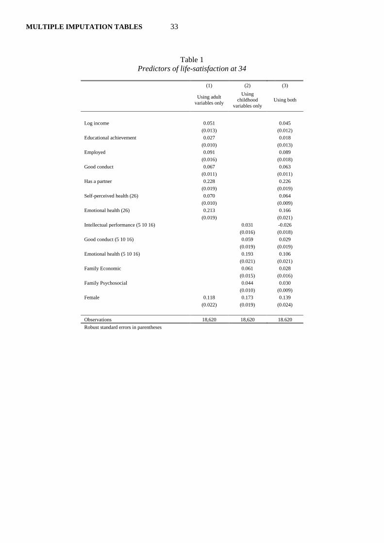
Table 1
Predictors of life-satisfaction at 34
(1) (2) (3)
Using adult
variables only
Using childhood
variables only
Using both
Log income 0.051
0.045
(0.013)
(0.012)
Educational achievement 0.027
0.018
(0.010)
(0.013)
Employed 0.091
0.089
(0.016)
(0.018)
Good conduct 0.067
0.063
(0.011)
(0.011)
Has a partner 0.228
0.226
(0.019)
(0.019)
Self-perceived health (26) 0.070
0.064
(0.010)
(0.009)
Emotional health (26) 0.213
0.166
(0.019)
(0.021)
Intellectual performance (5 10 16)
0.031 -0.026
(0.016) (0.018)
Good conduct (5 10 16)
0.059 0.029
(0.019) (0.019)
Emotional health (5 10 16)
0.193 0.106
(0.021) (0.021)
Family Economic
0.061 0.028
(0.015) (0.016)
Family Psychosocial
0.044 0.030
(0.010) (0.009)
Female 0.118 0.173 0.139
(0.022) (0.019) (0.024)
Observations 18,620 18,620 18.620
Robust standard errors in parentheses
MULTIPLE IMPUTATION TABLES 34
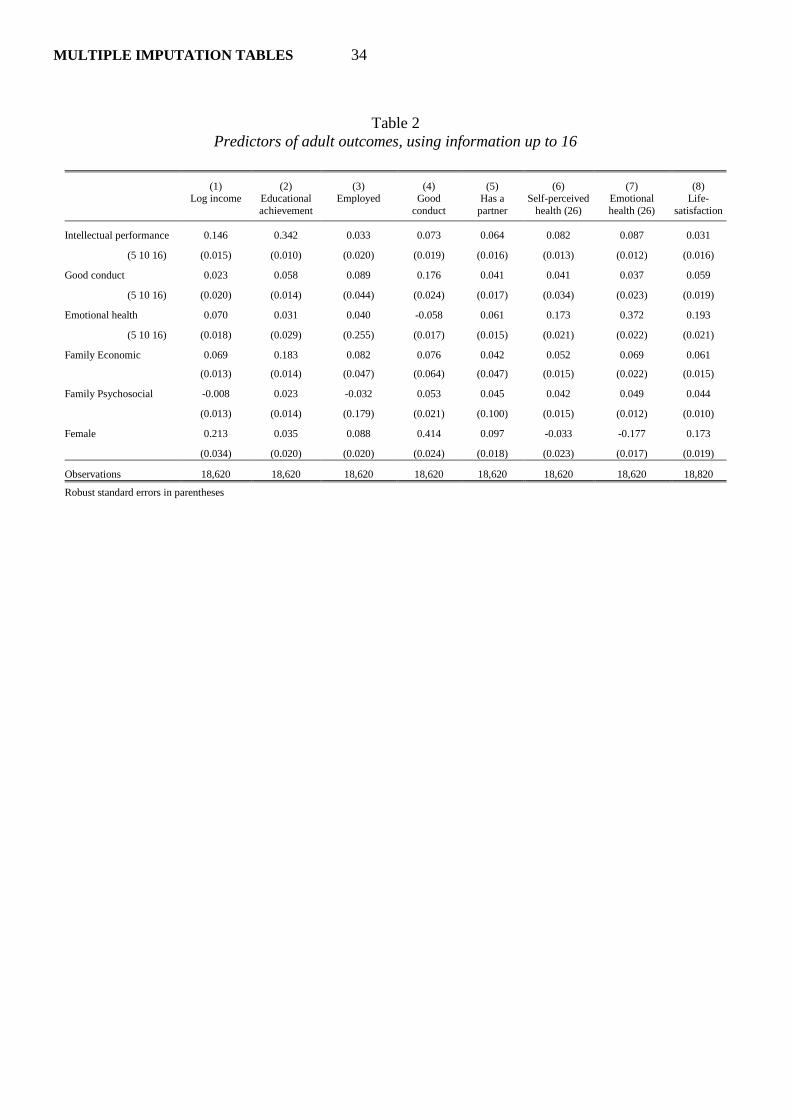
Table 2
Predictors of adult outcomes, using information up to 16
(1) (2) (3) (4) (5) (6) (7) (8)
Log income Educational
achievement
Employed Good
conduct
Has a
partner
Self-perceived
health (26)
Emotional
health (26)
Life-
satisfaction
Intellectual performance 0.146 0.342 0.033 0.073 0.064 0.082 0.087 0.031
(5 10 16) (0.015) (0.010) (0.020) (0.019) (0.016) (0.013) (0.012) (0.016)
Good conduct 0.023 0.058 0.089 0.176 0.041 0.041 0.037 0.059
(5 10 16) (0.020) (0.014) (0.044) (0.024) (0.017) (0.034) (0.023) (0.019)
Emotional health 0.070 0.031 0.040 -0.058 0.061 0.173 0.372 0.193
(5 10 16) (0.018) (0.029) (0.255) (0.017) (0.015) (0.021) (0.022) (0.021)
Family Economic 0.069 0.183 0.082 0.076 0.042 0.052 0.069 0.061
(0.013) (0.014) (0.047) (0.064) (0.047) (0.015) (0.022) (0.015)
Family Psychosocial -0.008 0.023 -0.032 0.053 0.045 0.042 0.049 0.044
(0.013) (0.014) (0.179) (0.021) (0.100) (0.015) (0.012) (0.010)
Female 0.213 0.035 0.088 0.414 0.097 -0.033 -0.177 0.173
(0.034) (0.020) (0.020) (0.024) (0.018) (0.023) (0.017) (0.019)
Observations 18,620 18,620 18,620 18,620 18,620 18,620 18,620 18,820
Robust standard errors in parentheses
MULTIPLE IMPUTATION TABLES 35
Table 3
Indirect effect of childhood variables upon life-
satisfaction at 34
(1) (2)
Simulated From Table 1
[Col (2) minus Col (3)]
Intellectual performance (5 10 16) 0.063 0.057
Good conduct (5 10 16) 0.043 0.030
Emotional health (5 10 16) 0.109 0.087
Family Economic 0.049 0.033
Family Psychosocial 0.024 0.014
MULTIPLE IMPUTATION TABLES 36
Table 4
Predictors of adult outcomes, using family only
(1) (2) (3) (4) (5) (6) (7) (8)
Log income Educational
achievement
Employed Good
conduct
Has a
partner
Self-perceived
health (26)
Emotional
health (26)
Life-
satisfaction
Family Economic 0.125 0.314 0.098 0.118 0.056 0.082 0.120 0.082
(0.019) (0.020) (0.046) (0.053) (0.025) (0.018) (0.033) (0.020)
Family Psychosocial 0.030 0.077 0.034 0.081 0.051 0.093 0.144 0.099
(0.011) (0.012) (0.050) (0.019) (0.021) (0.014) (0.012) (0.010)
Female 0.196 0.065 0.098 0.470 0.082 -0.090 -0.308 0.177
(0.032) (0.016) (0.028) (0.019) (0.018) (0.025) (0.021) (0.017)
Observations 18,620 18,620 18,620 18,620 18,620 18,620 18,620 18,620
Robust standard errors in parentheses
MULTIPLE IMPUTATION TABLES 37
Table B.1
Predictors of adult outcomes, using information up to 5
(1) (2) (3) (4) (5) (6) (7) (8)
Log income Educational
achievement
Employed Good
conduct
Has a
partner
Self-perceived
health (26)
Emotional
health (26)
Life-
satisfaction
Intellectual performance 0.079 0.159 0.025 0.044 0.049 0.056 0.068 0.043
(5) (0.009) (0.009) (0.019) (0.009) (0.014) (0.011) (0.009) (0.012)
Good conduct 0.033 0.053 0.026 0.095 0.032 0.020 0.042 0.039
(5) (0.014) (0.009) (0.029) (0.018) (0.012) (0.013) (0.016) (0.015)
Emotional health 0.015 0.014 -0.012 -0.038 0.016 0.033 0.057 0.026
(5) (0.012) (0.010) (0.010) (0.012) (0.019) (0.010) (0.013) (0.012)
Family Economic 0.103 0.269 0.090 0.098 0.046 0.067 0.102 0.069
(0.018) (0.017) (0.047) (0.070) (0.031) (0.017) (0.034) (0.018)
Family Psychosocial 0.012 0.048 0.033 0.068 0.046 0.074 0.107 0.077
(0.011) (0.013) (0.078) (0.020) (0.034) (0.016) (0.013) (0.009)
Female 0.188 0.052 0.091 0.445 0.074 -0.095 -0.321 0.106
(0.031) (0.018) (0.031) (0.017) (0.019) (0.023) (0.021) (0.017)
Observations 8,888 10,575 8,928 10,918 6,896 8,260 8,254 8,868
Adj R-square 0.029 0.176 0.008 0.043 0.016 0.027 0.061 0.022
Robust standard errors in parentheses
MULTIPLE IMPUTATION TABLES 38
Table B.2
Predictors of adult outcomes, using information up to 10
(1) (2) (3) (4) (5) (6) (7) (8)
Log income Educational
achievement
Employed Good
conduct
Has a
partner
Self-perceived
health (26)
Emotional
health (26)
Life-
satisfaction
Intellectual performance 0.124 0.256 0.031 0.042 0.069 0.069 0.095 0.044
(5 10) (0.012) (0.010) (0.004) (0.010) (0.015) (0.012) (0.010) (0.015)
Good conduct 0.028 0.079 0.024 0.129 0.031 0.022 0.056 0.062
(5 10) (0.017) (0.013) (0.006) (0.017) (0.013) (0.011) (0.020) (0.015)
Emotional health 0.016 -0.026 0.038 -0.053 0.033 0.056 0.080 0.040
(5 10) (0.014) (0.040) (0.011) (0.011) (0.015) (0.011) (0.011) (0.012)
Family Economic 0.079 0.210 0.088 0.091 0.041 0.058 0.086 0.065
(0.016) (0.016) (0.009) (0.072) (0.048) (0.017) (0.036) (0.018)
Family Psychosocial 0.009 0.035 0.037 0.064 0.047 0.060 0.081 0.061
(0.022) (0.013) (0.181) (0.021) (0.061) (0.014) (0.012) (0.009)
Female 0.195 0.052 0.096 0.425 0.078 -0.092 -0.321 0.098
(0.034) (0.018) (0.007) (0.017) (0.019) (0.024) (0.020) (0.017)
Observations 18,620 18,620 18,620 18,620 18,620 18,620 18,620 18,620
Robust standard errors in parentheses
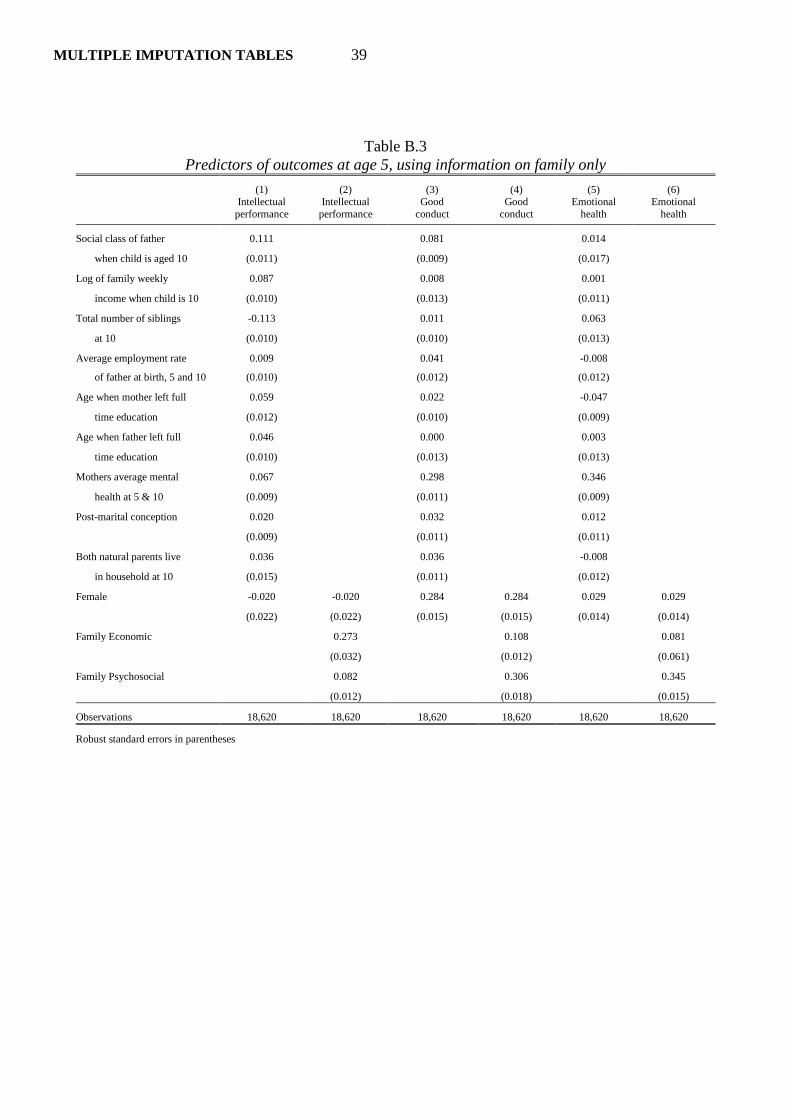
MULTIPLE IMPUTATION TABLES 39
Table B.3
Predictors of outcomes at age 5, using information on family only
(1) (2) (3) (4) (5) (6)
Intellectual
performance
Intellectual
performance
Good
conduct
Good
conduct
Emotional
health
Emotional
health
Social class of father 0.111
0.081
0.014
when child is aged 10 (0.011)
(0.009)
(0.017)
Log of family weekly 0.087
0.008
0.001
income when child is 10 (0.010)
(0.013)
(0.011)
Total number of siblings -0.113
0.011
0.063
at 10 (0.010)
(0.010)
(0.013)
Average employment rate 0.009
0.041
-0.008
of father at birth, 5 and 10 (0.010)
(0.012)
(0.012)
Age when mother left full 0.059
0.022
-0.047
time education (0.012)
(0.010)
(0.009)
Age when father left full 0.046
0.000
0.003
time education (0.010)
(0.013)
(0.013)
Mothers average mental 0.067 0.298 0.346
health at 5 & 10 (0.009) (0.011) (0.009)
Post-marital conception 0.020 0.032 0.012
(0.009) (0.011) (0.011)
Both natural parents live 0.036 0.036 -0.008
in household at 10 (0.015) (0.011) (0.012)
Female -0.020 -0.020 0.284 0.284 0.029 0.029
(0.022) (0.022) (0.015) (0.015) (0.014) (0.014)
Family Economic 0.273 0.108 0.081
(0.032) (0.012) (0.061)
Family Psychosocial 0.082 0.306 0.345
(0.012) (0.018) (0.015)
Observations 18,620 18,620 18,620 18,620 18,620 18,620
Robust standard errors in parentheses
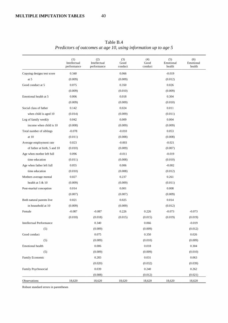
MULTIPLE IMPUTATION TABLES 40
Table B.4
Predictors of outcomes at age 10, using information up to age 5
(1) (2) (3) (4) (5) (6)
Intellectual performance
Intellectual performance
Good conduct
Good conduct
Emotional health
Emotional health
Copying designs test score 0.340 0.066 -0.019
at 5 (0.009) (0.009) (0.012)
Good conduct at 5 0.075 0.350 0.026
(0.009) (0.010) (0.009)
Emotional health at 5 0.006 0.018 0.304
(0.009) (0.009) (0.010)
Social class of father 0.142
0.024
0.011
when child is aged 10 (0.014)
(0.009)
(0.011)
Log of family weekly 0.042
0.009
0.004
income when child is 10 (0.008)
(0.009)
(0.009)
Total number of siblings -0.078
-0.010
0.053
at 10 (0.011)
(0.008)
(0.008)
Average employment rate 0.023
-0.003
-0.021
of father at birth, 5 and 10 (0.010)
(0.009)
(0.007)
Age when mother left full 0.096
-0.011
-0.019
time education (0.011)
(0.008)
(0.010)
Age when father left full 0.055
0.006
-0.002
time education (0.010)
(0.008)
(0.012)
Mothers average mental 0.027 0.237 0.261
health at 5 & 10 (0.009) (0.009) (0.011)
Post-marital conception 0.014 0.001 0.008
(0.007) (0.007) (0.009)
Both natural parents live 0.021 0.025 0.014
in household at 10 (0.009) (0.009) (0.012)
Female -0.087 -0.087 0.226 0.226 -0.073 -0.073
(0.018) (0.018) (0.015) (0.015) (0.019) (0.019)
Intellectual Performance 0.340 0.066 -0.019
(5) (0.009) (0.009) (0.012)
Good conduct 0.075 0.350 0.026
(5) (0.009) (0.010) (0.009)
Emotional health 0.006 0.018 0.304
(5) (0.009) (0.009) (0.010)
Family Economic 0.283 0.031 0.063
(0.020) (0.032) (0.039)
Family Psychosocial 0.039 0.240 0.262
(0.008) (0.012) (0.021)
Observations 18,620 18,620 18,620 18,620 18,620 18,620
Robust standard errors in parentheses
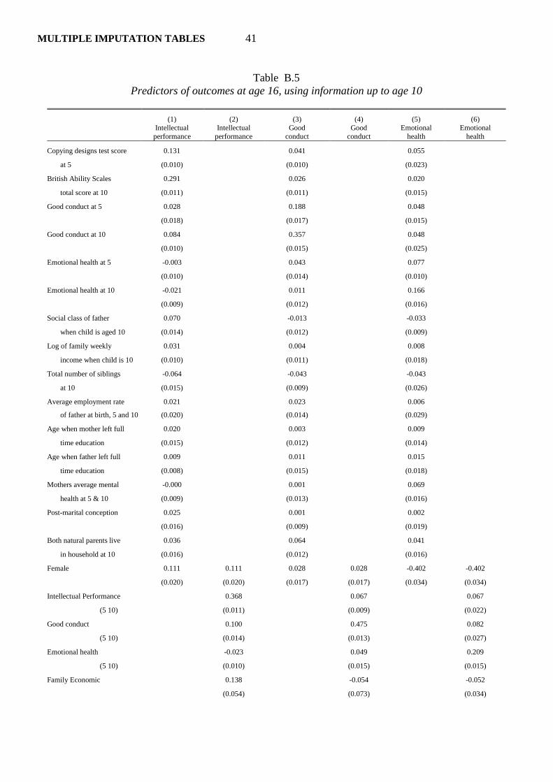
MULTIPLE IMPUTATION TABLES 41
Table B.5
Predictors of outcomes at age 16, using information up to age 10
(1) (2) (3) (4) (5) (6)
Intellectual
performance
Intellectual
performance
Good
conduct
Good
conduct
Emotional
health
Emotional
health
Copying designs test score 0.131 0.041 0.055
at 5 (0.010) (0.010) (0.023)
British Ability Scales 0.291 0.026 0.020
total score at 10 (0.011) (0.011) (0.015)
Good conduct at 5 0.028 0.188 0.048
(0.018) (0.017) (0.015)
Good conduct at 10 0.084 0.357 0.048
(0.010) (0.015) (0.025)
Emotional health at 5 -0.003 0.043 0.077
(0.010) (0.014) (0.010)
Emotional health at 10 -0.021 0.011 0.166
(0.009) (0.012) (0.016)
Social class of father 0.070
-0.013
-0.033
when child is aged 10 (0.014)
(0.012)
(0.009)
Log of family weekly 0.031
0.004
0.008
income when child is 10 (0.010)
(0.011)
(0.018)
Total number of siblings -0.064
-0.043
-0.043
at 10 (0.015)
(0.009)
(0.026)
Average employment rate 0.021
0.023
0.006
of father at birth, 5 and 10 (0.020)
(0.014)
(0.029)
Age when mother left full 0.020
0.003
0.009
time education (0.015)
(0.012)
(0.014)
Age when father left full 0.009
0.011
0.015
time education (0.008)
(0.015)
(0.018)
Mothers average mental -0.000 0.001 0.069
health at 5 & 10 (0.009) (0.013) (0.016)
Post-marital conception 0.025 0.001 0.002
(0.016) (0.009) (0.019)
Both natural parents live 0.036 0.064 0.041
in household at 10 (0.016) (0.012) (0.016)
Female 0.111 0.111 0.028 0.028 -0.402 -0.402
(0.020) (0.020) (0.017) (0.017) (0.034) (0.034)
Intellectual Performance 0.368 0.067 0.067
(5 10) (0.011) (0.009) (0.022)
Good conduct 0.100 0.475 0.082
(5 10) (0.014) (0.013) (0.027)
Emotional health -0.023 0.049 0.209
(5 10) (0.010) (0.015) (0.015)
Family Economic 0.138 -0.054 -0.052
(0.054) (0.073) (0.034)

MULTIPLE IMPUTATION TABLES 42
Family Psychosocial 0.045 0.064 0.084
(0.018) (0.023) (0.020)
Observations 18,620 18,620 18,620 18,620 8,089 8,089
Robust standard errors in parentheses
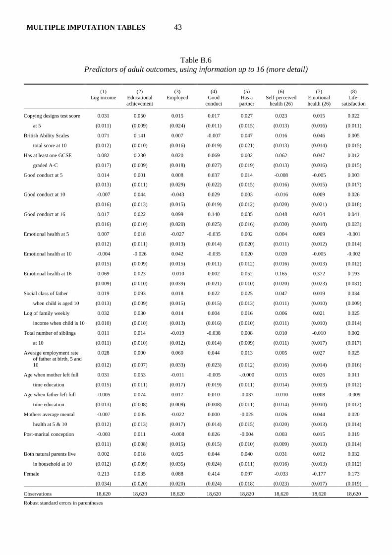
MULTIPLE IMPUTATION TABLES 43
Table B.6
Predictors of adult outcomes, using information up to 16 (more detail)
(1) (2) (3) (4) (5) (6) (7) (8)
Log income Educational
achievement
Employed Good
conduct
Has a
partner
Self-perceived
health (26)
Emotional
health (26)
Life-
satisfaction
Copying designs test score 0.031 0.050 0.015 0.017 0.027 0.023 0.015 0.022
at 5 (0.011) (0.009) (0.024) (0.011) (0.015) (0.013) (0.016) (0.011)
British Ability Scales 0.071 0.141 0.007 -0.007 0.047 0.016 0.046 0.005
total score at 10 (0.012) (0.010) (0.016) (0.019) (0.021) (0.013) (0.014) (0.015)
Has at least one GCSE 0.082 0.230 0.020 0.069 0.002 0.062 0.047 0.012
graded A-C (0.017) (0.009) (0.018) (0.027) (0.019) (0.013) (0.016) (0.015)
Good conduct at 5 0.014 0.001 0.008 0.037 0.014 -0.008 -0.005 0.003
(0.013) (0.011) (0.029) (0.022) (0.015) (0.016) (0.015) (0.017)
Good conduct at 10 -0.007 0.044 -0.043 0.029 0.003 -0.016 0.009 0.026
(0.016) (0.013) (0.015) (0.019) (0.012) (0.020) (0.021) (0.018)
Good conduct at 16 0.017 0.022 0.099 0.140 0.035 0.048 0.034 0.041
(0.016) (0.010) (0.020) (0.025) (0.016) (0.030) (0.018) (0.023)
Emotional health at 5 0.007 0.018 -0.027 -0.035 0.002 0.004 0.009 -0.001
(0.012) (0.011) (0.013) (0.014) (0.020) (0.011) (0.012) (0.014)
Emotional health at 10 -0.004 -0.026 0.042 -0.035 0.020 0.020 -0.005 -0.002
(0.015) (0.009) (0.015) (0.011) (0.012) (0.016) (0.013) (0.012)
Emotional health at 16 0.069 0.023 -0.010 0.002 0.052 0.165 0.372 0.193
(0.009) (0.010) (0.039) (0.021) (0.010) (0.020) (0.023) (0.031)
Social class of father 0.019 0.093 0.018 0.022 0.025 0.047 0.019 0.034
when child is aged 10 (0.013) (0.009) (0.015) (0.015) (0.013) (0.011) (0.010) (0.009)
Log of family weekly 0.032 0.030 0.014 0.004 0.016 0.006 0.021 0.025
income when child is 10 (0.010) (0.010) (0.013) (0.016) (0.010) (0.011) (0.010) (0.014)
Total number of siblings 0.011 0.014 -0.019 -0.038 0.008 0.010 -0.010 0.002
at 10 (0.011) (0.010) (0.012) (0.014) (0.009) (0.011) (0.017) (0.017)
Average employment rate 0.028 0.000 0.060 0.044 0.013 0.005 0.027 0.025 of father at birth, 5 and
10 (0.012) (0.007) (0.033) (0.023) (0.012) (0.016) (0.014) (0.016)
Age when mother left full 0.031 0.053 -0.011 -0.005 -.0.000 0.015 0.026 0.011
time education (0.015) (0.011) (0.017) (0.019) (0.011) (0.014) (0.013) (0.012)
Age when father left full -0.005 0.074 0.017 0.010 -0.037 -0.010 0.008 -0.009
time education (0.013) (0.008) (0.009) (0.008) (0.011) (0.014) (0.010) (0.012)
Mothers average mental -0.007 0.005 -0.022 0.000 -0.025 0.026 0.044 0.020
health at 5 & 10 (0.012) (0.013) (0.017) (0.014) (0.015) (0.020) (0.013) (0.014)
Post-marital conception -0.003 0.011 -0.008 0.026 -0.004 0.003 0.015 0.019
(0.011) (0.008) (0.015) (0.015) (0.010) (0.009) (0.013) (0.014)
Both natural parents live 0.002 0.018 0.025 0.044 0.040 0.031 0.012 0.032
in household at 10 (0.012) (0.009) (0.035) (0.024) (0.011) (0.016) (0.013) (0.012)
Female 0.213 0.035 0.088 0.414 0.097 -0.033 -0.177 0.173
(0.034) (0.020) (0.020) (0.024) (0.018) (0.023) (0.017) (0.019)
Observations 18,620 18,620 18,620 18,620 18,820 18,620 18,620 18,620
Robust standard errors in parentheses
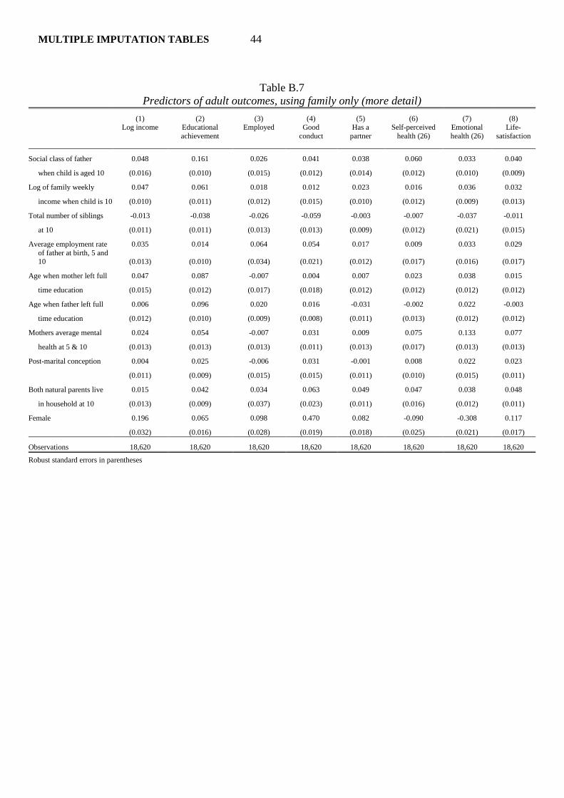
MULTIPLE IMPUTATION TABLES 44
Table B.7
Predictors of adult outcomes, using family only (more detail)
(1) (2) (3) (4) (5) (6) (7) (8)
Log income Educational
achievement
Employed Good
conduct
Has a
partner
Self-perceived
health (26)
Emotional
health (26)
Life-
satisfaction
Social class of father 0.048 0.161 0.026 0.041 0.038 0.060 0.033 0.040
when child is aged 10 (0.016) (0.010) (0.015) (0.012) (0.014) (0.012) (0.010) (0.009)
Log of family weekly 0.047 0.061 0.018 0.012 0.023 0.016 0.036 0.032
income when child is 10 (0.010) (0.011) (0.012) (0.015) (0.010) (0.012) (0.009) (0.013)
Total number of siblings -0.013 -0.038 -0.026 -0.059 -0.003 -0.007 -0.037 -0.011
at 10 (0.011) (0.011) (0.013) (0.013) (0.009) (0.012) (0.021) (0.015)
Average employment rate 0.035 0.014 0.064 0.054 0.017 0.009 0.033 0.029
of father at birth, 5 and 10 (0.013) (0.010) (0.034) (0.021) (0.012) (0.017) (0.016) (0.017)
Age when mother left full 0.047 0.087 -0.007 0.004 0.007 0.023 0.038 0.015
time education (0.015) (0.012) (0.017) (0.018) (0.012) (0.012) (0.012) (0.012)
Age when father left full 0.006 0.096 0.020 0.016 -0.031 -0.002 0.022 -0.003
time education (0.012) (0.010) (0.009) (0.008) (0.011) (0.013) (0.012) (0.012)
Mothers average mental 0.024 0.054 -0.007 0.031 0.009 0.075 0.133 0.077
health at 5 & 10 (0.013) (0.013) (0.013) (0.011) (0.013) (0.017) (0.013) (0.013)
Post-marital conception 0.004 0.025 -0.006 0.031 -0.001 0.008 0.022 0.023
(0.011) (0.009) (0.015) (0.015) (0.011) (0.010) (0.015) (0.011)
Both natural parents live 0.015 0.042 0.034 0.063 0.049 0.047 0.038 0.048
in household at 10 (0.013) (0.009) (0.037) (0.023) (0.011) (0.016) (0.012) (0.011)
Female 0.196 0.065 0.098 0.470 0.082 -0.090 -0.308 0.117
(0.032) (0.016) (0.028) (0.019) (0.018) (0.025) (0.021) (0.017)
Observations 18,620 18,620 18,620 18,620 18,620 18,620 18,620 18,620
Robust standard errors in parentheses
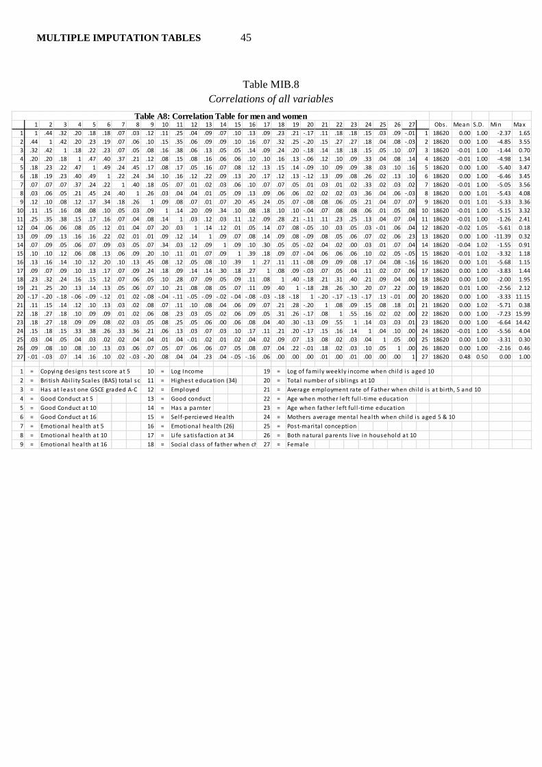
MULTIPLE IMPUTATION TABLES 45
Table MIB.8
Correlations of all variables
1 2 3 4 5 6 7 8 9 10 11 12 13 14 15 16 17 18 19 20 21 22 23 24 25 26 27 Obs. Mean S.D. Min Max
1 1 .44 .32 .20 .18 .18 .07 .03 .12 .11 .25 .04 .09 .07 .10 .13 .09 .23 .21 -.17 .11 .18 .18 .15 .03 .09 -.01 1 18620 0.00 1.00 -2.37 1.65
2 .44 1 .42 .20 .23 .19 .07 .06 .10 .15 .35 .06 .09 .09 .10 .16 .07 .32 .25 -.20 .15 .27 .27 .18 .04 .08 -.03 2 18620 0.00 1.00 -4.85 3.55
3 .32 .42 1 .18 .22 .23 .07 .05 .08 .16 .38 .06 .13 .05 .05 .14 .09 .24 .20 -.18 .14 .18 .18 .15 .05 .10 .07 3 18620 -0.01 1.00 -1.44 0.70
4 .20 .20 .18 1 .47 .40 .37 .21 .12 .08 .15 .08 .16 .06 .06 .10 .10 .16 .13 -.06 .12 .10 .09 .33 .04 .08 .14 4 18620 -0.01 1.00 -4.98 1.34
5 .18 .23 .22 .47 1 .49 .24 .45 .17 .08 .17 .05 .16 .07 .08 .12 .13 .15 .14 -.09 .10 .09 .09 .38 .03 .10 .16 5 18620 0.00 1.00 -5.40 3.47
6 .18 .19 .23 .40 .49 1 .22 .24 .34 .10 .16 .12 .22 .09 .13 .20 .17 .12 .13 -.12 .13 .09 .08 .26 .02 .13 .10 6 18620 0.00 1.00 -6.46 3.45
7 .07 .07 .07 .37 .24 .22 1 .40 .18 .05 .07 .01 .02 .03 .06 .10 .07 .07 .05 .01 .03 .01 .02 .33 .02 .03 .02 7 18620 -0.01 1.00 -5.05 3.56
8 .03 .06 .05 .21 .45 .24 .40 1 .26 .03 .04 .04 .01 .05 .09 .13 .09 .06 .06 .02 .02 .02 .03 .36 .04 .06 -.03 8 18620 0.00 1.01 -5.43 4.08
9 .12 .10 .08 .12 .17 .34 .18 .26 1 .09 .08 .07 .01 .07 .20 .45 .24 .05 .07 -.08 .08 .06 .05 .21 .04 .07 .07 9 18620 0.01 1.01 -5.33 3.36
10 .11 .15 .16 .08 .08 .10 .05 .03 .09 1 .14 .20 .09 .34 .10 .08 .18 .10 .10 -.04 .07 .08 .08 .06 .01 .05 .08 10 18620 -0.01 1.00 -5.15 3.32
11 .25 .35 .38 .15 .17 .16 .07 .04 .08 .14 1 .03 .12 .03 .11 .12 .09 .28 .21 -.11 .11 .23 .25 .13 .04 .07 .04 11 18620 -0.01 1.00 -1.26 2.41
12 .04 .06 .06 .08 .05 .12 .01 .04 .07 .20 .03 1 .14 .12 .01 .05 .14 .07 .08 -.05 .10 .03 .05 .03 -.01 .06 .04 12 18620 -0.02 1.05 -5.61 0.18
13 .09 .09 .13 .16 .16 .22 .02 .01 .01 .09 .12 .14 1 .09 .07 .08 .14 .09 .08 -.09 .08 .05 .06 .07 .02 .06 .23 13 18620 0.00 1.00 -11.39 0.32
14 .07 .09 .05 .06 .07 .09 .03 .05 .07 .34 .03 .12 .09 1 .09 .10 .30 .05 .05 -.02 .04 .02 .00 .03 .01 .07 .04 14 18620 -0.04 1.02 -1.55 0.91
15 .10 .10 .12 .06 .08 .13 .06 .09 .20 .10 .11 .01 .07 .09 1 .39 .18 .09 .07 -.04 .06 .06 .06 .10 .02 .05 -.05 15 18620 -0.01 1.02 -3.32 1.18
16 .13 .16 .14 .10 .12 .20 .10 .13 .45 .08 .12 .05 .08 .10 .39 1 .27 .11 .11 -.08 .09 .09 .08 .17 .04 .08 -.16 16 18620 0.00 1.01 -5.68 1.15
17 .09 .07 .09 .10 .13 .17 .07 .09 .24 .18 .09 .14 .14 .30 .18 .27 1 .08 .09 -.03 .07 .05 .04 .11 .02 .07 .06 17 18620 0.00 1.00 -3.83 1.44
18 .23 .32 .24 .16 .15 .12 .07 .06 .05 .10 .28 .07 .09 .05 .09 .11 .08 1 .40 -.18 .21 .31 .40 .21 .09 .04 .00 18 18620 0.00 1.00 -2.00 1.95
19 .21 .25 .20 .13 .14 .13 .05 .06 .07 .10 .21 .08 .08 .05 .07 .11 .09 .40 1 -.18 .28 .26 .30 .20 .07 .22 .00 19 18620 0.01 1.00 -2.56 2.12
20 -.17 -.20 -.18 -.06 -.09 -.12 .01 .02 -.08 -.04 -.11 -.05 -.09 -.02 -.04 -.08 -.03 -.18 -.18 1 -.20 -.17 -.13 -.17 .13 -.01 .00 20 18620 0.00 1.00 -3.33 11.15
21 .11 .15 .14 .12 .10 .13 .03 .02 .08 .07 .11 .10 .08 .04 .06 .09 .07 .21 .28 -.20 1 .08 .09 .15 .08 .18 .01 21 18620 0.00 1.02 -5.71 0.38
22 .18 .27 .18 .10 .09 .09 .01 .02 .06 .08 .23 .03 .05 .02 .06 .09 .05 .31 .26 -.17 .08 1 .55 .16 .02 .02 .00 22 18620 0.00 1.00 -7.23 15.99
23 .18 .27 .18 .09 .09 .08 .02 .03 .05 .08 .25 .05 .06 .00 .06 .08 .04 .40 .30 -.13 .09 .55 1 .14 .03 .03 .01 23 18620 0.00 1.00 -6.64 14.42
24 .15 .18 .15 .33 .38 .26 .33 .36 .21 .06 .13 .03 .07 .03 .10 .17 .11 .21 .20 -.17 .15 .16 .14 1 .04 .10 .00 24 18620 -0.01 1.00 -5.56 4.04
25 .03 .04 .05 .04 .03 .02 .02 .04 .04 .01 .04 -.01 .02 .01 .02 .04 .02 .09 .07 .13 .08 .02 .03 .04 1 .05 .00 25 18620 0.00 1.00 -3.31 0.30
26 .09 .08 .10 .08 .10 .13 .03 .06 .07 .05 .07 .06 .06 .07 .05 .08 .07 .04 .22 -.01 .18 .02 .03 .10 .05 1 .00 26 18620 0.00 1.00 -2.16 0.46
27 -.01 -.03 .07 .14 .16 .10 .02 -.03 -.20 .08 .04 .04 .23 .04 -.05 -.16 .06 .00 .00 .00 .01 .00 .01 .00 .00 .00 1 27 18620 0.48 0.50 0.00 1.00
1 = Copying des igns test score at 5 10 = Log Income 19 = Log of fami ly weekly income when chi ld i s aged 10
2 = Bri tish Abi l i ty Sca les (BAS) tota l score at 1011 = Highest education (34) 20 = Total number of s ibl ings at 10
3 = Has at least one GSCE graded A-C 12 = Employed 21 = Average employment rate of Father when chi ld i s at bi rth, 5 and 10
4 = Good Conduct at 5 13 = Good conduct 22 = Age when mother left ful l -time education
5 = Good Conduct at 10 14 = Has a parnter 23 = Age when father left ful l -time education
6 = Good Conduct at 16 15 = Sel f-percieved Health 24 = Mothers average mental health when chi ld i s aged 5 & 10
7 = Emotional health at 5 16 = Emotional health (26) 25 = Post-mari ta l conception
8 = Emotional health at 10 17 = Li fe satis faction at 34 26 = Both natura l parents l ive in household at 10
9 = Emotional health at 16 18 = Socia l class of father when chi ld i s aged 1027 = Female
Table A8: Correlation Table for men and women
46
QUESTIONNAIRES
1. Adult outcomes
2. Family variables
3. Intellectual performance
4. Good conduct
5. Emotional health
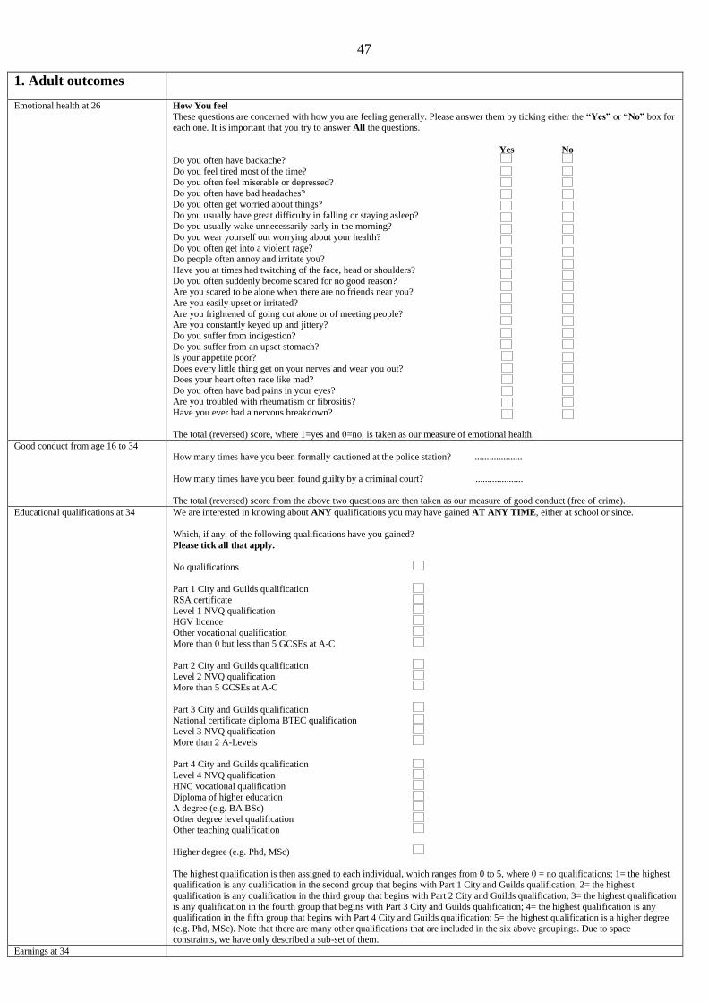
47
1. Adult outcomes
Emotional health at 26 How You feel
These questions are concerned with how you are feeling generally. Please answer them by ticking either the “Yes” or “No” box for each one. It is important that you try to answer All the questions.
Yes No
Do you often have backache?
Do you feel tired most of the time?
Do you often feel miserable or depressed? Do you often have bad headaches?
Do you often get worried about things?
Do you usually have great difficulty in falling or staying asleep? Do you usually wake unnecessarily early in the morning?
Do you wear yourself out worrying about your health?
Do you often get into a violent rage? Do people often annoy and irritate you?
Have you at times had twitching of the face, head or shoulders? Do you often suddenly become scared for no good reason? Are you scared to be alone when there are no friends near you?
Are you easily upset or irritated?
Are you frightened of going out alone or of meeting people? Are you constantly keyed up and jittery?
Do you suffer from indigestion? Do you suffer from an upset stomach?
Is your appetite poor?
Does every little thing get on your nerves and wear you out? Does your heart often race like mad?
Do you often have bad pains in your eyes?
Are you troubled with rheumatism or fibrositis? Have you ever had a nervous breakdown?
The total (reversed) score, where 1=yes and 0=no, is taken as our measure of emotional health.
Good conduct from age 16 to 34 How many times have you been formally cautioned at the police station? ....................
How many times have you been found guilty by a criminal court? ....................
The total (reversed) score from the above two questions are then taken as our measure of good conduct (free of crime).
Educational qualifications at 34 We are interested in knowing about ANY qualifications you may have gained AT ANY TIME, either at school or since.
Which, if any, of the following qualifications have you gained?
Please tick all that apply.
No qualifications
Part 1 City and Guilds qualification
RSA certificate
Level 1 NVQ qualification HGV licence
Other vocational qualification
More than 0 but less than 5 GCSEs at A-C
Part 2 City and Guilds qualification
Level 2 NVQ qualification More than 5 GCSEs at A-C
Part 3 City and Guilds qualification National certificate diploma BTEC qualification
Level 3 NVQ qualification
More than 2 A-Levels
Part 4 City and Guilds qualification
Level 4 NVQ qualification HNC vocational qualification
Diploma of higher education
A degree (e.g. BA BSc) Other degree level qualification
Other teaching qualification
Higher degree (e.g. Phd, MSc)
The highest qualification is then assigned to each individual, which ranges from 0 to 5, where 0 = no qualifications; 1= the highest qualification is any qualification in the second group that begins with Part 1 City and Guilds qualification; 2= the highest
qualification is any qualification in the third group that begins with Part 2 City and Guilds qualification; 3= the highest qualification is any qualification in the fourth group that begins with Part 3 City and Guilds qualification; 4= the highest qualification is any
qualification in the fifth group that begins with Part 4 City and Guilds qualification; 5= the highest qualification is a higher degree
(e.g. Phd, MSc). Note that there are many other qualifications that are included in the six above groupings. Due to space constraints, we have only described a sub-set of them.
Earnings at 34
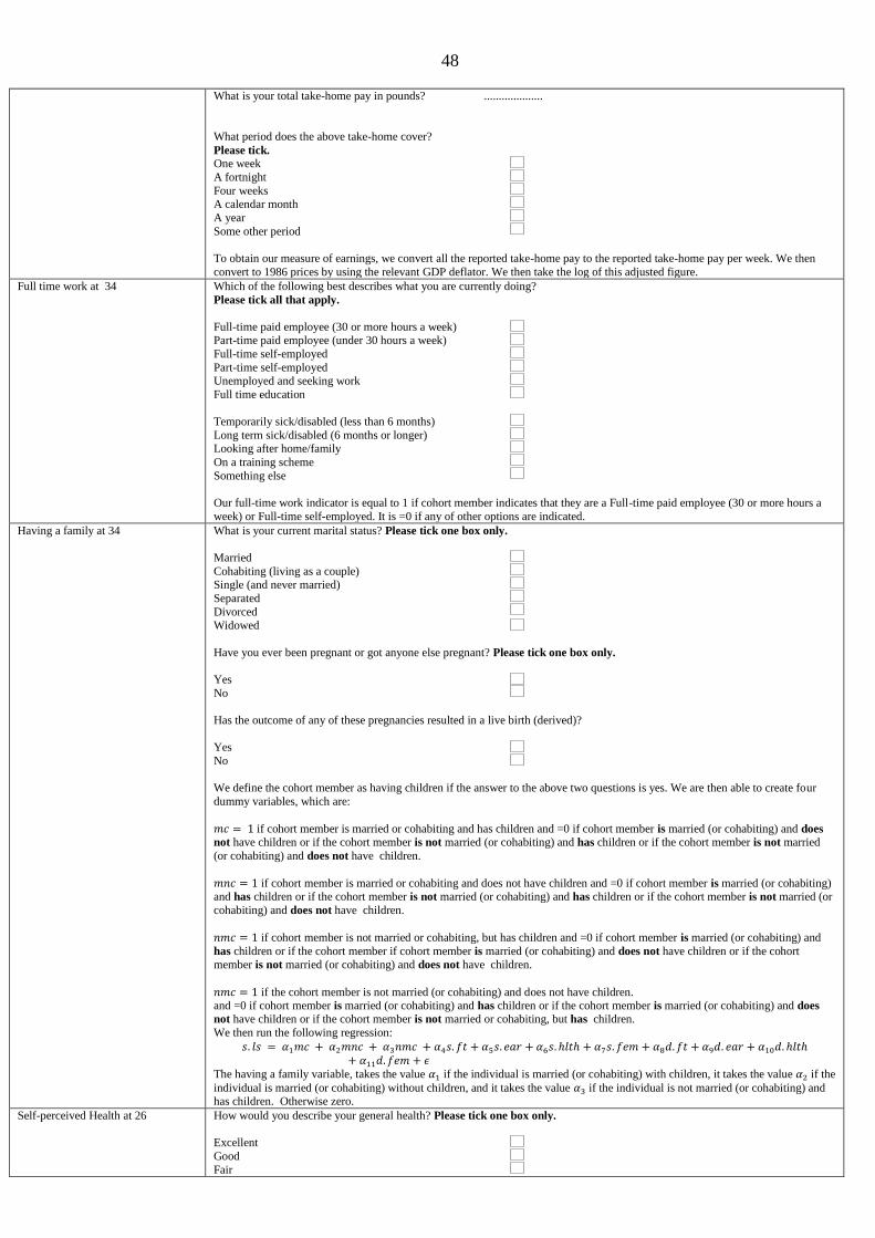
48
What is your total take-home pay in pounds? ....................
What period does the above take-home cover?
Please tick.
One week
A fortnight
Four weeks A calendar month
A year
Some other period
To obtain our measure of earnings, we convert all the reported take-home pay to the reported take-home pay per week. We then
convert to 1986 prices by using the relevant GDP deflator. We then take the log of this adjusted figure.
Full time work at 34 Which of the following best describes what you are currently doing?
Please tick all that apply.
Full-time paid employee (30 or more hours a week) Part-time paid employee (under 30 hours a week)
Full-time self-employed
Part-time self-employed Unemployed and seeking work
Full time education
Temporarily sick/disabled (less than 6 months)
Long term sick/disabled (6 months or longer) Looking after home/family
On a training scheme
Something else
Our full-time work indicator is equal to 1 if cohort member indicates that they are a Full-time paid employee (30 or more hours a
week) or Full-time self-employed. It is =0 if any of other options are indicated.
Having a family at 34 What is your current marital status? Please tick one box only.
Married
Cohabiting (living as a couple) Single (and never married)
Separated
Divorced Widowed
Have you ever been pregnant or got anyone else pregnant? Please tick one box only.
Yes
No
Has the outcome of any of these pregnancies resulted in a live birth (derived)?
Yes
No
We define the cohort member as having children if the answer to the above two questions is yes. We are then able to create four
dummy variables, which are:
if cohort member is married or cohabiting and has children and =0 if cohort member is married (or cohabiting) and does
not have children or if the cohort member is not married (or cohabiting) and has children or if the cohort member is not married
(or cohabiting) and does not have children.
if cohort member is married or cohabiting and does not have children and =0 if cohort member is married (or cohabiting) and has children or if the cohort member is not married (or cohabiting) and has children or if the cohort member is not married (or
cohabiting) and does not have children.
if cohort member is not married or cohabiting, but has children and =0 if cohort member is married (or cohabiting) and
has children or if the cohort member if cohort member is married (or cohabiting) and does not have children or if the cohort
member is not married (or cohabiting) and does not have children.
if the cohort member is not married (or cohabiting) and does not have children. and =0 if cohort member is married (or cohabiting) and has children or if the cohort member is married (or cohabiting) and does not have children or if the cohort member is not married or cohabiting, but has children.
We then run the following regression:
The having a family variable, takes the value if the individual is married (or cohabiting) with children, it takes the value if the
individual is married (or cohabiting) without children, and it takes the value if the individual is not married (or cohabiting) and has children. Otherwise zero.
Self-perceived Health at 26 How would you describe your general health? Please tick one box only.
Excellent
Good
Fair
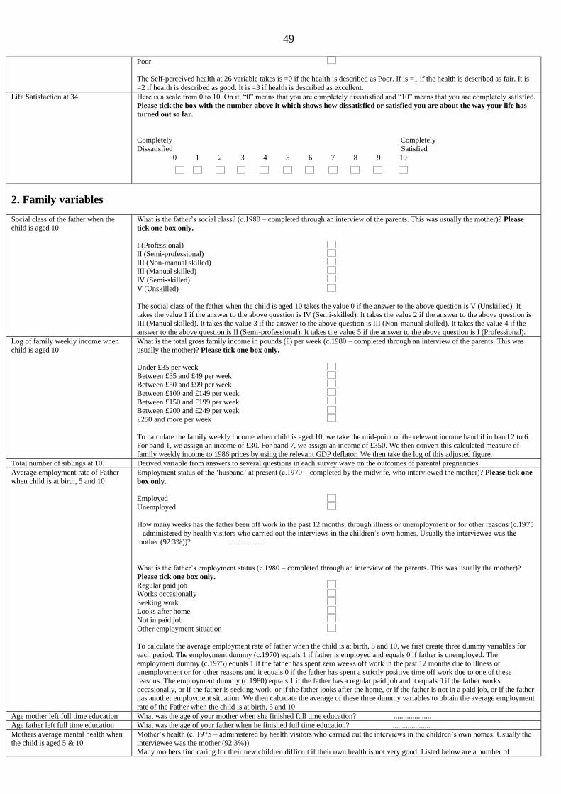
49
Poor
The Self-perceived health at 26 variable takes is =0 if the health is described as Poor. If is =1 if the health is described as fair. It is
=2 if health is described as good. It is =3 if health is described as excellent.
Life Satisfaction at 34 Here is a scale from 0 to 10. On it, “0” means that you are completely dissatisfied and “10” means that you are completely satisfied.
Please tick the box with the number above it which shows how dissatisfied or satisfied you are about the way your life has
turned out so far.
Completely Completely
Dissatisfied Satisfied
0 1 2 3 4 5 6 7 8 9 10
2. Family variables
Social class of the father when the child is aged 10
What is the father’s social class? (c.1980 – completed through an interview of the parents. This was usually the mother)? Please
tick one box only.
I (Professional) II (Semi-professional)
III (Non-manual skilled) III (Manual skilled)
IV (Semi-skilled)
V (Unskilled)
The social class of the father when the child is aged 10 takes the value 0 if the answer to the above question is V (Unskilled). It
takes the value 1 if the answer to the above question is IV (Semi-skilled). It takes the value 2 if the answer to the above question is III (Manual skilled). It takes the value 3 if the answer to the above question is III (Non-manual skilled). It takes the value 4 if the
answer to the above question is II (Semi-professional). It takes the value 5 if the answer to the above question is I (Professional).
Log of family weekly income when
child is aged 10
What is the total gross family income in pounds (£) per week (c.1980 – completed through an interview of the parents. This was
usually the mother)? Please tick one box only.
Under £35 per week
Between £35 and £49 per week Between £50 and £99 per week
Between £100 and £149 per week
Between £150 and £199 per week Between £200 and £249 per week
£250 and more per week
To calculate the family weekly income when child is aged 10, we take the mid-point of the relevant income band if in band 2 to 6.
For band 1, we assign an income of £30. For band 7, we assign an income of £350. We then convert this calculated measure of
family weekly income to 1986 prices by using the relevant GDP deflator. We then take the log of this adjusted figure.
Total number of siblings at 10. Derived variable from answers to several questions in each survey wave on the outcomes of parental pregnancies.
Average employment rate of Father
when child is at birth, 5 and 10
Employment status of the ‘husband’ at present (c.1970 – completed by the midwife, who interviewed the mother)? Please tick one
box only.
Employed
Unemployed
How many weeks has the father been off work in the past 12 months, through illness or unemployment or for other reasons (c.1975
– administered by health visitors who carried out the interviews in the children’s own homes. Usually the interviewee was the mother (92.3%))? ....................
What is the father’s employment status (c.1980 – completed through an interview of the parents. This was usually the mother)?
Please tick one box only.
Regular paid job Works occasionally
Seeking work
Looks after home
Not in paid job
Other employment situation
To calculate the average employment rate of father when the child is at birth, 5 and 10, we first create three dummy variables for
each period. The employment dummy (c.1970) equals 1 if father is employed and equals 0 if father is unemployed. The
employment dummy (c.1975) equals 1 if the father has spent zero weeks off work in the past 12 months due to illness or unemployment or for other reasons and it equals 0 if the father has spent a strictly positive time off work due to one of these
reasons. The employment dummy (c.1980) equals 1 if the father has a regular paid job and it equals 0 if the father works
occasionally, or if the father is seeking work, or if the father looks after the home, or if the father is not in a paid job, or if the father has another employment situation. We then calculate the average of these three dummy variables to obtain the average employment
rate of the Father when the child is at birth, 5 and 10.
Age mother left full time education What was the age of your mother when she finished full time education? ....................
Age father left full time education What was the age of your father when he finished full time education? ....................
Mothers average mental health when
the child is aged 5 & 10
Mother’s health (c. 1975 – administered by health visitors who carried out the interviews in the children’s own homes. Usually the
interviewee was the mother (92.3%))
Many mothers find caring for their new children difficult if their own health is not very good. Listed below are a number of
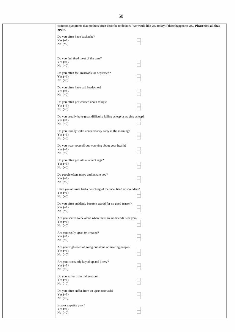
50
common symptoms that mothers often describe to doctors. We would like you to say if these happen to you. Please tick all that
apply.
Do you often have backache?
Yes (=1) No (=0)
Do you feel tired most of the time?
Yes (=1) No (=0)
Do you often feel miserable or depressed? Yes (=1)
No (=0)
Do you often have bad headaches?
Yes (=1)
No (=0)
Do you often get worried about things?
Yes (=1)
No (=0)
Do you usually have great difficulty falling asleep or staying asleep? Yes (=1)
No (=0)
Do you usually wake unnecessarily early in the morning?
Yes (=1)
No (=0)
Do you wear yourself out worrying about your health?
Yes (=1) No (=0)
Do you often get into a violent rage? Yes (=1)
No (=0)
Do people often annoy and irritate you?
Yes (=1)
No (=0)
Have you at times had a twitching of the face, head or shoulders?
Yes (=1) No (=0)
Do you often suddenly become scared for no good reason? Yes (=1)
No (=0)
Are you scared to be alone when there are no friends near you?
Yes (=1) No (=0)
Are you easily upset or irritated? Yes (=1)
No (=0)
Are you frightened of going out alone or meeting people?
Yes (=1)
No (=0)
Are you constantly keyed up and jittery?
Yes (=1) No (=0)
Do you suffer from indigestion? Yes (=1)
No (=0)
Do you often suffer from an upset stomach?
Yes (=1)
No (=0)
Is your appetite poor?
Yes (=1) No (=0)
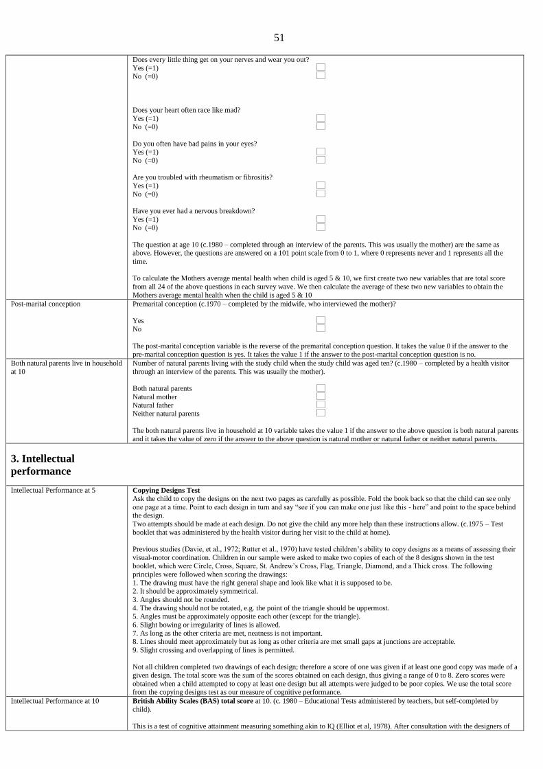
51
Does every little thing get on your nerves and wear you out?
Yes (=1) No (=0)
Does your heart often race like mad?
Yes (=1) No (=0)
Do you often have bad pains in your eyes? Yes (=1)
No (=0)
Are you troubled with rheumatism or fibrositis?
Yes (=1)
No (=0)
Have you ever had a nervous breakdown?
Yes (=1) No (=0)
The question at age 10 (c.1980 – completed through an interview of the parents. This was usually the mother) are the same as
above. However, the questions are answered on a 101 point scale from 0 to 1, where 0 represents never and 1 represents all the
time.
To calculate the Mothers average mental health when child is aged 5 & 10, we first create two new variables that are total score
from all 24 of the above questions in each survey wave. We then calculate the average of these two new variables to obtain the
Mothers average mental health when the child is aged 5 & 10
Post-marital conception Premarital conception (c.1970 – completed by the midwife, who interviewed the mother)?
Yes No
The post-marital conception variable is the reverse of the premarital conception question. It takes the value 0 if the answer to the pre-marital conception question is yes. It takes the value 1 if the answer to the post-marital conception question is no.
Both natural parents live in household
at 10
Number of natural parents living with the study child when the study child was aged ten? (c.1980 – completed by a health visitor
through an interview of the parents. This was usually the mother).
Both natural parents
Natural mother
Natural father Neither natural parents
The both natural parents live in household at 10 variable takes the value 1 if the answer to the above question is both natural parents and it takes the value of zero if the answer to the above question is natural mother or natural father or neither natural parents.
3. Intellectual
performance
Intellectual Performance at 5 Copying Designs Test
Ask the child to copy the designs on the next two pages as carefully as possible. Fold the book back so that the child can see only
one page at a time. Point to each design in turn and say “see if you can make one just like this - here” and point to the space behind the design.
Two attempts should be made at each design. Do not give the child any more help than these instructions allow. (c.1975 – Test
booklet that was administered by the health visitor during her visit to the child at home).
Previous studies (Davie, et al., 1972; Rutter et al., 1970) have tested children’s ability to copy designs as a means of assessing their
visual-motor coordination. Children in our sample were asked to make two copies of each of the 8 designs shown in the test booklet, which were Circle, Cross, Square, St. Andrew’s Cross, Flag, Triangle, Diamond, and a Thick cross. The following
principles were followed when scoring the drawings:
1. The drawing must have the right general shape and look like what it is supposed to be. 2. It should be approximately symmetrical.
3. Angles should not be rounded.
4. The drawing should not be rotated, e.g. the point of the triangle should be uppermost. 5. Angles must be approximately opposite each other (except for the triangle).
6. Slight bowing or irregularity of lines is allowed.
7. As long as the other criteria are met, neatness is not important. 8. Lines should meet approximately but as long as other criteria are met small gaps at junctions are acceptable.
9. Slight crossing and overlapping of lines is permitted.
Not all children completed two drawings of each design; therefore a score of one was given if at least one good copy was made of a
given design. The total score was the sum of the scores obtained on each design, thus giving a range of 0 to 8. Zero scores were
obtained when a child attempted to copy at least one design but all attempts were judged to be poor copies. We use the total score from the copying designs test as our measure of cognitive performance.
Intellectual Performance at 10 British Ability Scales (BAS) total score at 10. (c. 1980 – Educational Tests administered by teachers, but self-completed by
child).
This is a test of cognitive attainment measuring something akin to IQ (Elliot et al, 1978). After consultation with the designers of
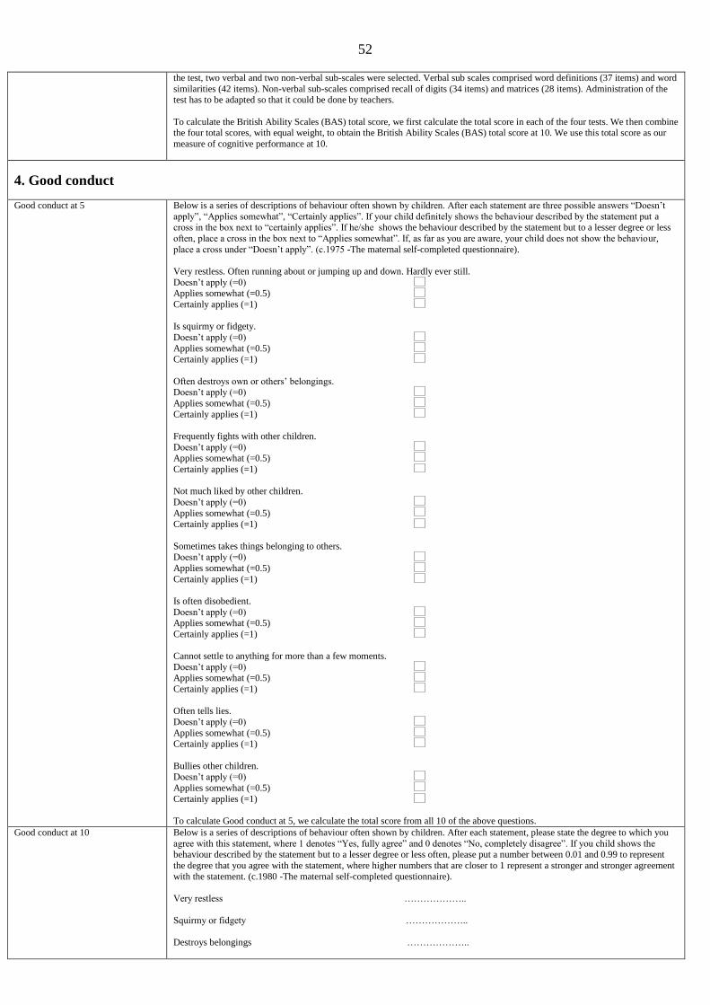
52
the test, two verbal and two non-verbal sub-scales were selected. Verbal sub scales comprised word definitions (37 items) and word
similarities (42 items). Non-verbal sub-scales comprised recall of digits (34 items) and matrices (28 items). Administration of the test has to be adapted so that it could be done by teachers.
To calculate the British Ability Scales (BAS) total score, we first calculate the total score in each of the four tests. We then combine the four total scores, with equal weight, to obtain the British Ability Scales (BAS) total score at 10. We use this total score as our
measure of cognitive performance at 10.
4. Good conduct
Good conduct at 5 Below is a series of descriptions of behaviour often shown by children. After each statement are three possible answers “Doesn’t
apply”, “Applies somewhat”, “Certainly applies”. If your child definitely shows the behaviour described by the statement put a cross in the box next to “certainly applies”. If he/she shows the behaviour described by the statement but to a lesser degree or less
often, place a cross in the box next to “Applies somewhat”. If, as far as you are aware, your child does not show the behaviour,
place a cross under “Doesn’t apply”. (c.1975 -The maternal self-completed questionnaire).
Very restless. Often running about or jumping up and down. Hardly ever still.
Doesn’t apply (=0) Applies somewhat (=0.5)
Certainly applies (=1)
Is squirmy or fidgety.
Doesn’t apply (=0)
Applies somewhat (=0.5) Certainly applies (=1)
Often destroys own or others’ belongings. Doesn’t apply (=0)
Applies somewhat (=0.5)
Certainly applies (=1)
Frequently fights with other children.
Doesn’t apply (=0) Applies somewhat (=0.5)
Certainly applies (=1)
Not much liked by other children.
Doesn’t apply (=0)
Applies somewhat (=0.5) Certainly applies (=1)
Sometimes takes things belonging to others.
Doesn’t apply (=0)
Applies somewhat (=0.5)
Certainly applies (=1)
Is often disobedient.
Doesn’t apply (=0) Applies somewhat (=0.5)
Certainly applies (=1)
Cannot settle to anything for more than a few moments.
Doesn’t apply (=0) Applies somewhat (=0.5)
Certainly applies (=1)
Often tells lies.
Doesn’t apply (=0)
Applies somewhat (=0.5) Certainly applies (=1)
Bullies other children.
Doesn’t apply (=0)
Applies somewhat (=0.5)
Certainly applies (=1)
To calculate Good conduct at 5, we calculate the total score from all 10 of the above questions.
Good conduct at 10 Below is a series of descriptions of behaviour often shown by children. After each statement, please state the degree to which you
agree with this statement, where 1 denotes “Yes, fully agree” and 0 denotes “No, completely disagree”. If you child shows the behaviour described by the statement but to a lesser degree or less often, please put a number between 0.01 and 0.99 to represent
the degree that you agree with the statement, where higher numbers that are closer to 1 represent a stronger and stronger agreement
with the statement. (c.1980 -The maternal self-completed questionnaire).
Very restless ………………..
Squirmy or fidgety ………………..
Destroys belongings ………………..
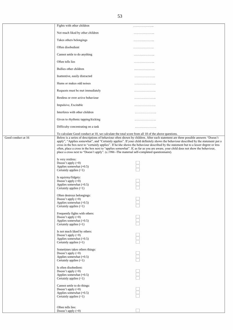
53
Fights with other children ………………..
Not much liked by other children ………………..
Takes others belongings ………………..
Often disobedient ………………..
Cannot settle to do anything ………………..
Often tells lies ………………..
Bullies other children ………………..
Inattentive, easily distracted ………………..
Hums or makes odd noises .………………..
Requests must be met immediately .………………..
Restless or over active behaviour .………………..
Impulsive, Excitable .………………..
Interferes with other children .………………..
Given to rhythmic tapping/kicking .………………..
Difficulty concentrating on a task .………………..
To calculate Good conduct at 10, we calculate the total score from all 18 of the above questions.
Good conduct at 16 Below is a series of descriptions of behaviour often shown by children. After each statement are three possible answers “Doesn’t apply”, “Applies somewhat”, and “Certainly applies”. If your child definitely shows the behaviour described by the statement put a
cross in the box next to “certainly applies”. If he/she shows the behaviour described by the statement but to a lesser degree or less
often, place a cross in the box next to “applies somewhat”. If, as far as you are aware, your child does not show the behaviour, place a cross next to “Doesn’t apply”. (c.1986 -The maternal self-completed questionnaire).
Is very restless: Doesn’t apply (=0)
Applies somewhat (=0.5)
Certainly applies (=1)
Is squirmy/fidgety:
Doesn’t apply (=0)
Applies somewhat (=0.5)
Certainly applies (=1)
Often destroys belongings:
Doesn’t apply (=0)
Applies somewhat (=0.5) Certainly applies (=1)
Frequently fights with others: Doesn’t apply (=0)
Applies somewhat (=0.5)
Certainly applies (=1)
Is not much liked by others:
Doesn’t apply (=0) Applies somewhat (=0.5)
Certainly applies (=1)
Sometimes takes others things:
Doesn’t apply (=0)
Applies somewhat (=0.5) Certainly applies (=1)
Is often disobedient: Doesn’t apply (=0)
Applies somewhat (=0.5)
Certainly applies (=1)
Cannot settle to do things:
Doesn’t apply (=0) Applies somewhat (=0.5)
Certainly applies (=1)
Often tells lies: Doesn’t apply (=0)
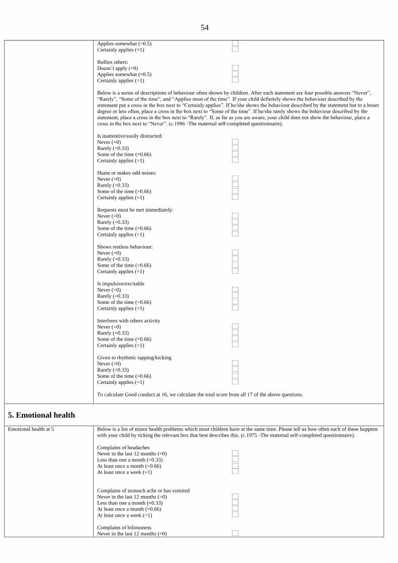
54
Applies somewhat (=0.5)
Certainly applies (=1)
Bullies others:
Doesn’t apply (=0) Applies somewhat (=0.5)
Certainly applies (=1)
Below is a series of descriptions of behaviour often shown by children. After each statement are four possible answers “Never”,
“Rarely”, “Some of the time”, and “Applies most of the time”. If your child definitely shows the behaviour described by the
statement put a cross in the box next to “Certainly applies”. If he/she shows the behaviour described by the statement but to a lesser degree or less often, place a cross in the box next to “Some of the time”. If he/she rarely shows the behaviour described by the
statement, place a cross in the box next to “Rarely”. If, as far as you are aware, your child does not show the behaviour, place a
cross in the box next to “Never”. (c.1986 -The maternal self-completed questionnaire).
Is inattentive/easily distracted:
Never (=0) Rarely (=0.33)
Some of the time (=0.66)
Certainly applies (=1)
Hums or makes odd noises:
Never (=0)
Rarely (=0.33)
Some of the time (=0.66)
Certainly applies (=1)
Requests must be met immediately:
Never (=0) Rarely (=0.33)
Some of the time (=0.66)
Certainly applies (=1)
Shows restless behaviour:
Never (=0) Rarely (=0.33)
Some of the time (=0.66)
Certainly applies (=1)
Is impulsive/excitable
Never (=0) Rarely (=0.33)
Some of the time (=0.66)
Certainly applies (=1)
Interferes with others activity
Never (=0) Rarely (=0.33)
Some of the time (=0.66)
Certainly applies (=1)
Given to rhythmic tapping/kicking Never (=0)
Rarely (=0.33)
Some of the time (=0.66) Certainly applies (=1)
To calculate Good conduct at 16, we calculate the total score from all 17 of the above questions.
5. Emotional health
Emotional health at 5 Below is a list of minor health problems which most children have at the same time. Please tell us how often each of these happens
with your child by ticking the relevant box that best describes this. (c.1975 -The maternal self-completed questionnaire).
Complains of headaches Never in the last 12 months (=0)
Less than one a month (=0.33)
At least once a month (=0.66) At least once a week (=1)
Complains of stomach ache or has vomited
Never in the last 12 months (=0)
Less than one a month (=0.33) At least once a month (=0.66)
At least once a week (=1)
Complains of biliousness
Never in the last 12 months (=0)
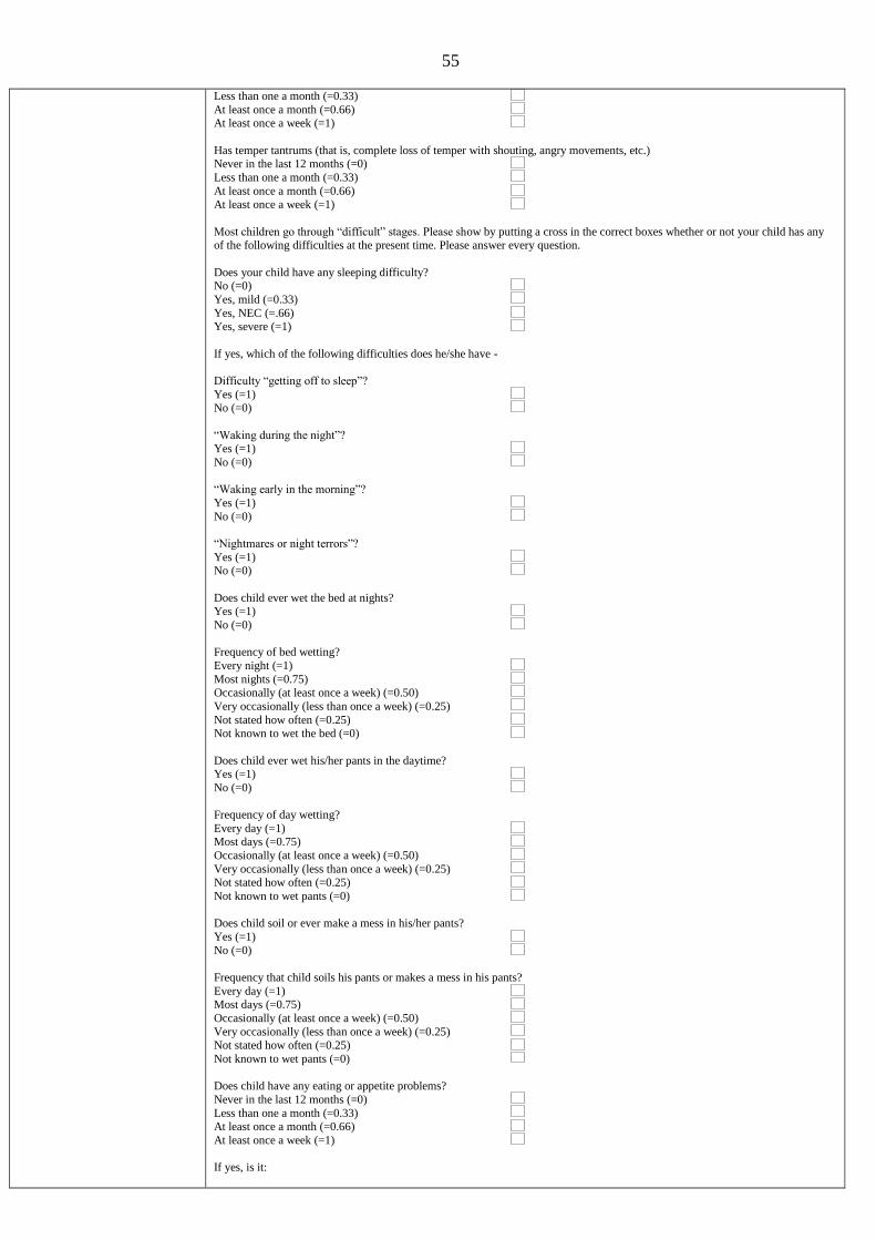
55
Less than one a month (=0.33)
At least once a month (=0.66) At least once a week (=1)
Has temper tantrums (that is, complete loss of temper with shouting, angry movements, etc.) Never in the last 12 months (=0)
Less than one a month (=0.33)
At least once a month (=0.66) At least once a week (=1)
Most children go through “difficult” stages. Please show by putting a cross in the correct boxes whether or not your child has any of the following difficulties at the present time. Please answer every question.
Does your child have any sleeping difficulty? No (=0)
Yes, mild (=0.33)
Yes, NEC (=.66) Yes, severe (=1)
If yes, which of the following difficulties does he/she have -
Difficulty “getting off to sleep”?
Yes (=1)
No (=0)
“Waking during the night”? Yes (=1)
No (=0)
“Waking early in the morning”?
Yes (=1)
No (=0)
“Nightmares or night terrors”?
Yes (=1) No (=0)
Does child ever wet the bed at nights? Yes (=1)
No (=0)
Frequency of bed wetting?
Every night (=1)
Most nights (=0.75)
Occasionally (at least once a week) (=0.50)
Very occasionally (less than once a week) (=0.25)
Not stated how often (=0.25) Not known to wet the bed (=0)
Does child ever wet his/her pants in the daytime? Yes (=1)
No (=0)
Frequency of day wetting?
Every day (=1) Most days (=0.75)
Occasionally (at least once a week) (=0.50)
Very occasionally (less than once a week) (=0.25) Not stated how often (=0.25)
Not known to wet pants (=0)
Does child soil or ever make a mess in his/her pants?
Yes (=1)
No (=0)
Frequency that child soils his pants or makes a mess in his pants?
Every day (=1) Most days (=0.75)
Occasionally (at least once a week) (=0.50)
Very occasionally (less than once a week) (=0.25) Not stated how often (=0.25)
Not known to wet pants (=0)
Does child have any eating or appetite problems?
Never in the last 12 months (=0)
Less than one a month (=0.33) At least once a month (=0.66)
At least once a week (=1)
If yes, is it:
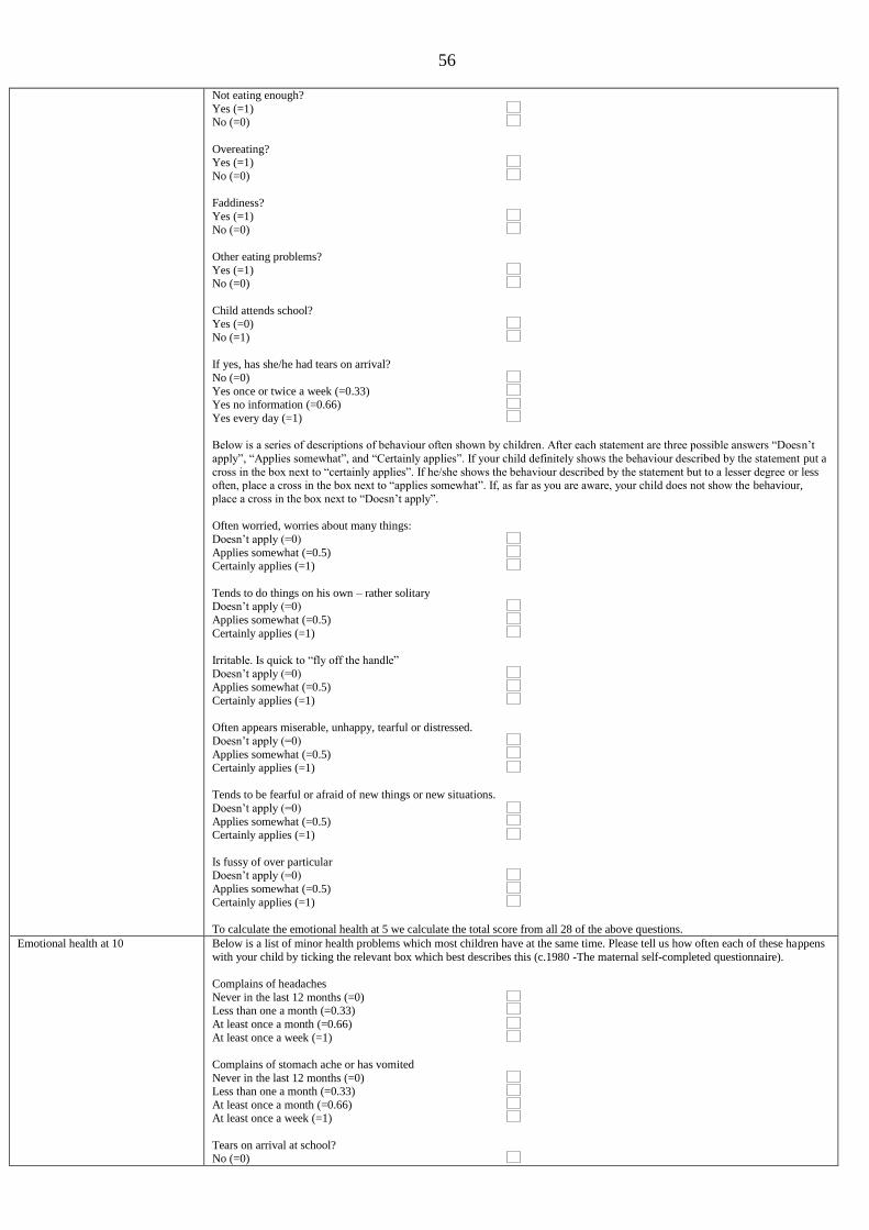
56
Not eating enough?
Yes (=1) No (=0)
Overeating? Yes (=1)
No (=0)
Faddiness?
Yes (=1)
No (=0)
Other eating problems?
Yes (=1) No (=0)
Child attends school? Yes (=0)
No (=1)
If yes, has she/he had tears on arrival?
No (=0)
Yes once or twice a week (=0.33)
Yes no information (=0.66)
Yes every day (=1)
Below is a series of descriptions of behaviour often shown by children. After each statement are three possible answers “Doesn’t
apply”, “Applies somewhat”, and “Certainly applies”. If your child definitely shows the behaviour described by the statement put a
cross in the box next to “certainly applies”. If he/she shows the behaviour described by the statement but to a lesser degree or less often, place a cross in the box next to “applies somewhat”. If, as far as you are aware, your child does not show the behaviour,
place a cross in the box next to “Doesn’t apply”.
Often worried, worries about many things:
Doesn’t apply (=0)
Applies somewhat (=0.5) Certainly applies (=1)
Tends to do things on his own – rather solitary Doesn’t apply (=0)
Applies somewhat (=0.5)
Certainly applies (=1)
Irritable. Is quick to “fly off the handle”
Doesn’t apply (=0)
Applies somewhat (=0.5)
Certainly applies (=1)
Often appears miserable, unhappy, tearful or distressed.
Doesn’t apply (=0)
Applies somewhat (=0.5) Certainly applies (=1)
Tends to be fearful or afraid of new things or new situations.
Doesn’t apply (=0)
Applies somewhat (=0.5) Certainly applies (=1)
Is fussy of over particular Doesn’t apply (=0)
Applies somewhat (=0.5)
Certainly applies (=1)
To calculate the emotional health at 5 we calculate the total score from all 28 of the above questions.
Emotional health at 10 Below is a list of minor health problems which most children have at the same time. Please tell us how often each of these happens
with your child by ticking the relevant box which best describes this (c.1980 -The maternal self-completed questionnaire).
Complains of headaches
Never in the last 12 months (=0) Less than one a month (=0.33)
At least once a month (=0.66)
At least once a week (=1)
Complains of stomach ache or has vomited
Never in the last 12 months (=0) Less than one a month (=0.33)
At least once a month (=0.66) At least once a week (=1)
Tears on arrival at school? No (=0)
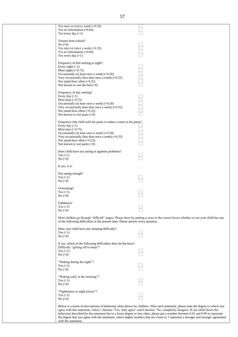
57
Yes once or twice a week (=0.33)
Yes no information (=0.66) Yes every day (=1)
Truants from school? No (=0)
Yes once or twice a week (=0.33)
Yes no information (=0.66) Yes every day (=1)
Frequency of bed wetting at night? Every night (=1)
Most nights (=0.75)
Occasionally (at least once a week) (=0.50) Very occasionally (less than once a week) (=0.25)
Not stated how often (=0.25)
Not known to wet the bed (=0)
Frequency of day wetting?
Every day (=1) Most days (=0.75)
Occasionally (at least once a week) (=0.50)
Very occasionally (less than once a week) (=0.25)
Not stated how often (=0.25)
Not known to wet pants (=0)
Frequency that child soils his pants or makes a mess in his pants?
Every day (=1)
Most days (=0.75) Occasionally (at least once a week) (=0.50)
Very occasionally (less than once a week) (=0.25)
Not stated how often (=0.25) Not known to wet pants (=0)
Does child have any eating or appetite problems? Yes (=1)
No (=0)
If yes, is it:
Not eating enough? Yes (=1)
No (=0)
Overeating?
Yes (=1)
No (=0)
Faddiness?
Yes (=1) No (=0)
Most children go through “difficult” stages. Please show by putting a cross in the correct boxes whether or not your child has any
of the following difficulties at the present time. Please answer every question.
Does your child have any sleeping difficulty?
Yes (=1)
No (=0)
If yes, which of the following difficulties does he/she have?
Difficulty “getting off to sleep”? Yes (=1)
No (=0)
“Waking during the night”?
Yes (=1)
No (=0)
“Waking early in the morning”?
Yes (=1) No (=0)
“Nightmares or night terrors”? Yes (=1)
No (=0)
Below is a series of descriptions of behaviour often shown by children. After each statement, please state the degree to which you
agree with this statement, where 1 denotes “Yes, fully agree” and 0 denotes “No, completely disagree. If you child shows the
behaviour described by the statement but to a lesser degree or less often, please put a number between 0.01 and 0.99 to represent the degree that you agree with the statement, where higher numbers that are closer to 1 represent a stronger and stronger agreement
with the statement.
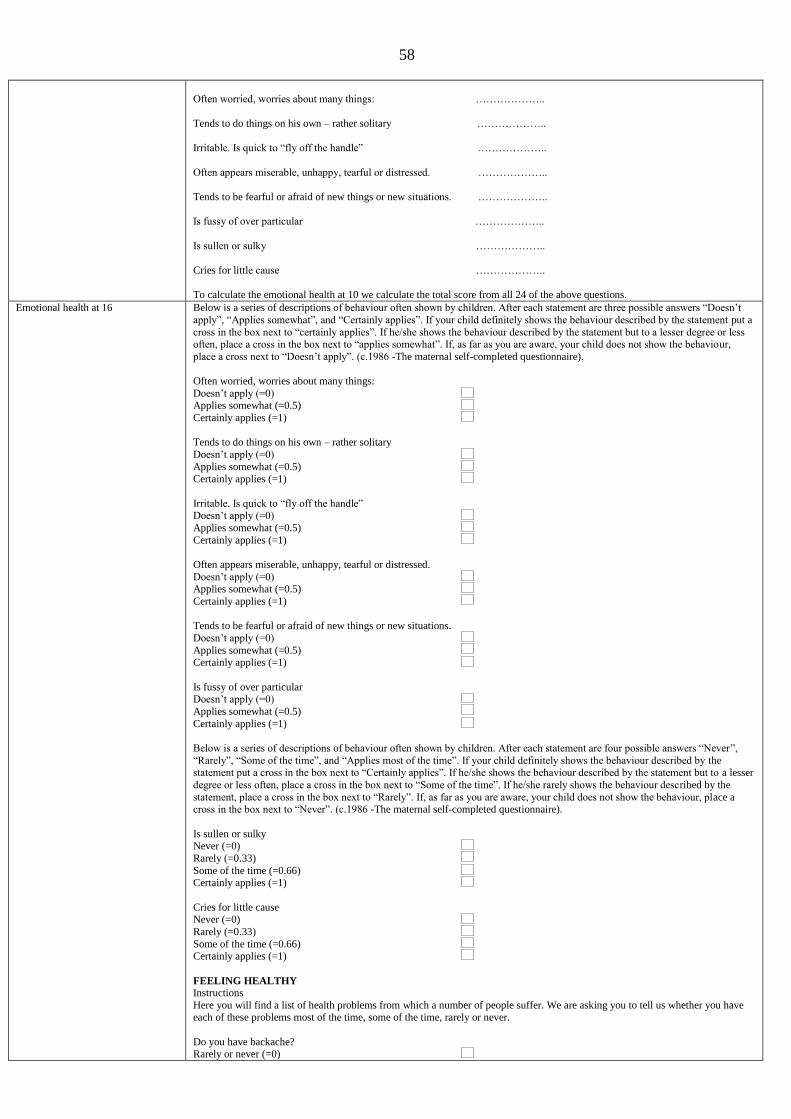
58
Often worried, worries about many things: ………………..
Tends to do things on his own – rather solitary ………………..
Irritable. Is quick to “fly off the handle” ………………..
Often appears miserable, unhappy, tearful or distressed. ………………..
Tends to be fearful or afraid of new things or new situations. ………………..
Is fussy of over particular ………………..
Is sullen or sulky ………………..
Cries for little cause ………………..
To calculate the emotional health at 10 we calculate the total score from all 24 of the above questions.
Emotional health at 16 Below is a series of descriptions of behaviour often shown by children. After each statement are three possible answers “Doesn’t
apply”, “Applies somewhat”, and “Certainly applies”. If your child definitely shows the behaviour described by the statement put a
cross in the box next to “certainly applies”. If he/she shows the behaviour described by the statement but to a lesser degree or less often, place a cross in the box next to “applies somewhat”. If, as far as you are aware, your child does not show the behaviour,
place a cross next to “Doesn’t apply”. (c.1986 -The maternal self-completed questionnaire).
Often worried, worries about many things:
Doesn’t apply (=0) Applies somewhat (=0.5)
Certainly applies (=1)
Tends to do things on his own – rather solitary
Doesn’t apply (=0)
Applies somewhat (=0.5) Certainly applies (=1)
Irritable. Is quick to “fly off the handle” Doesn’t apply (=0)
Applies somewhat (=0.5)
Certainly applies (=1)
Often appears miserable, unhappy, tearful or distressed.
Doesn’t apply (=0) Applies somewhat (=0.5)
Certainly applies (=1)
Tends to be fearful or afraid of new things or new situations.
Doesn’t apply (=0)
Applies somewhat (=0.5) Certainly applies (=1)
Is fussy of over particular Doesn’t apply (=0)
Applies somewhat (=0.5)
Certainly applies (=1)
Below is a series of descriptions of behaviour often shown by children. After each statement are four possible answers “Never”,
“Rarely”, “Some of the time”, and “Applies most of the time”. If your child definitely shows the behaviour described by the statement put a cross in the box next to “Certainly applies”. If he/she shows the behaviour described by the statement but to a lesser
degree or less often, place a cross in the box next to “Some of the time”. If he/she rarely shows the behaviour described by the
statement, place a cross in the box next to “Rarely”. If, as far as you are aware, your child does not show the behaviour, place a cross in the box next to “Never”. (c.1986 -The maternal self-completed questionnaire).
Is sullen or sulky Never (=0)
Rarely (=0.33)
Some of the time (=0.66) Certainly applies (=1)
Cries for little cause Never (=0)
Rarely (=0.33)
Some of the time (=0.66) Certainly applies (=1)
FEELING HEALTHY
Instructions
Here you will find a list of health problems from which a number of people suffer. We are asking you to tell us whether you have each of these problems most of the time, some of the time, rarely or never.
Do you have backache? Rarely or never (=0)
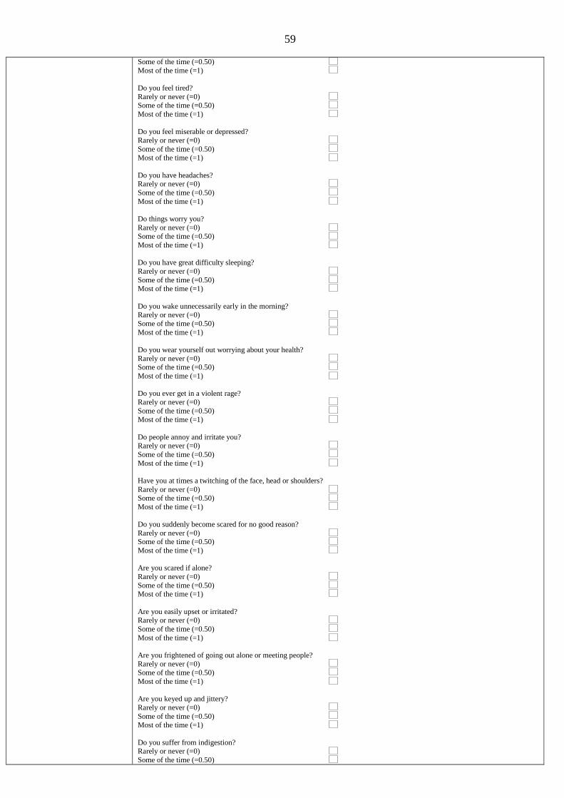
59
Some of the time (=0.50)
Most of the time (=1)
Do you feel tired?
Rarely or never (=0) Some of the time (=0.50)
Most of the time (=1)
Do you feel miserable or depressed?
Rarely or never (=0)
Some of the time (=0.50) Most of the time (=1)
Do you have headaches? Rarely or never (=0)
Some of the time (=0.50)
Most of the time (=1)
Do things worry you?
Rarely or never (=0) Some of the time (=0.50)
Most of the time (=1)
Do you have great difficulty sleeping?
Rarely or never (=0)
Some of the time (=0.50) Most of the time (=1)
Do you wake unnecessarily early in the morning? Rarely or never (=0)
Some of the time (=0.50)
Most of the time (=1)
Do you wear yourself out worrying about your health?
Rarely or never (=0) Some of the time (=0.50)
Most of the time (=1)
Do you ever get in a violent rage?
Rarely or never (=0)
Some of the time (=0.50) Most of the time (=1)
Do people annoy and irritate you?
Rarely or never (=0)
Some of the time (=0.50)
Most of the time (=1)
Have you at times a twitching of the face, head or shoulders?
Rarely or never (=0) Some of the time (=0.50)
Most of the time (=1)
Do you suddenly become scared for no good reason?
Rarely or never (=0) Some of the time (=0.50)
Most of the time (=1)
Are you scared if alone?
Rarely or never (=0)
Some of the time (=0.50) Most of the time (=1)
Are you easily upset or irritated?
Rarely or never (=0)
Some of the time (=0.50)
Most of the time (=1)
Are you frightened of going out alone or meeting people?
Rarely or never (=0) Some of the time (=0.50)
Most of the time (=1)
Are you keyed up and jittery?
Rarely or never (=0)
Some of the time (=0.50) Most of the time (=1)
Do you suffer from indigestion? Rarely or never (=0)
Some of the time (=0.50)
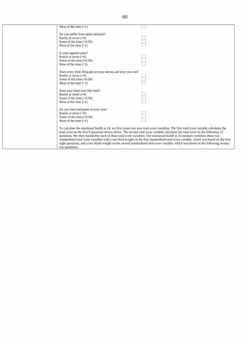
60
Most of the time (=1)
Do you suffer from upset stomach?
Rarely or never (=0)
Some of the time (=0.50) Most of the time (=1)
Is your appetite poor? Rarely or never (=0)
Some of the time (=0.50)
Most of the time (=1)
Does every little thing get on your nerves and wear you out?
Rarely or never (=0) Some of the time (=0.50)
Most of the time (=1)
Does your heart race like mad?
Rarely or never (=0)
Some of the time (=0.50) Most of the time (=1)
Do you have bad pains in your eyes?
Rarely or never (=0)
Some of the time (=0.50)
Most of the time (=1)
To calculate the emotional health at 16, we first create two new total score variables. The first total score variable calculates the
total score on the first 8 questions shown above. The second total score variable calculates the total score on the following 22 questions. We then standardise each of these total score variables. Our emotional health at 16 measure combines these two
standardised total score variables with a one third weight on the first standardised total score variable, which was based on the first
eight questions, and a two thirds weight on the second standardised total score variable, which was based on the following twenty-two questions.

61

CENTRE FOR ECONOMIC PERFORMANCE Recent Discussion Papers
1244 Benjamin Faber Trade Integration, Market Size and Industrialization: Evidence from China’s National Trunk Highway System
1243 Scott R Baker Nicholas Bloom
Does Uncertainty Reduce Growth? Using Disasters as Natural Experiments
1242 Jo Blanden Paul Gregg Lindsey Macmillan
Intergenerational Persistence in Income and Social Class: The Impact of Within-Group Inequality
1241 Richard Murphy Felix Weinhardt
The Importance of Rank Position
1240 Alex Eble Peter Boone Diana Elbourne
Risk and Evidence of Bias in Randomized Controlled Trials in Economics
1239 Richard Layard Dan Chisholm Vikram Patel Shekhar Saxena
Mental Illness and Unhappiness
1238 Laura Jaitman Stephen Machin
Crime and Immigration: New Evidence from England and Wales
1237 Ross Levine Yona Rubinstein
Smart and Illicit: Who Becomes an Entrepreneur and Does it Pay?
1236 Jan-Emmanuel De Neve Ed Diener Louis Tay Cody Xuereb
The Objective Benefits of Subjective Well-Being
1235 Pascal Michaillat Emmanuel Saez
A Model of Aggregate Demand and Unemployment
1234 Jerónimo Carballo, Gianmarco I.P. Ottaviano Christian Volpe Martincus
The Buyer Margins of Firms’ Exports
1233 Daniel Fujiwara A General Method for Valuing Non-Market Goods Using Wellbeing Data: Three-Stage Wellbeing Valuation
1232 Holger Breinlich Gianmarco I. P. Ottaviano Jonathan R. W. Temple
Regional Growth and Regional Decline
1231 Michalis Drouvelis Nattavudh Powdthavee
Are Happier People Less Judgmental of Other People's Selfish Behaviors? Laboratory Evidence from Trust and Gift Exchange Games
1230 Dan Anderberg Helmut Rainer Jonathan Wadsworth Tanya Wilson
Unemployment and Domestic Violence: Theory and Evidence
1229 Hannes Schwandt Unmet Aspirations as an Explanation for the Age U-Shape in Human Wellbeing
1228 Bénédicte Apouey Andrew E. Clark
Winning Big But Feeling No Better? The Effect of Lottery Prizes on Physical and Mental Health
1227 Alex Gyani Roz Shafran Richard Layard David M Clark
Enhancing Recovery Rates: Lessons from Year One of the English Improving Access to Psychological Therapies Programme
1226 Stephen Gibbons Sandra McNally
The Effects of Resources Across School Phases: A Summary of Recent Evidence
1225 Cornelius A. Rietveld David Cesarini Daniel J. Benjamin Philipp D. Koellinger Jan-Emmanuel De Neve Henning Tiemeier Magnus Johannesson Patrik K.E. Magnusson Nancy L. Pedersen Robert F. Krueger Meike Bartels
Molecular Genetics and Subjective Well-Being
1224 Peter Arcidiacono Esteban Aucejo Patrick Coate V. Joseph Hotz
Affirmative Action and University Fit: Evidence from Proposition 209
1223 Peter Arcidiacono Esteban Aucejo V. Joseph Hotz
University Differences in the Graduation of Minorities in STEM Fields: Evidence from California
1222 Paul Dolan Robert Metcalfe
Neighbors, Knowledge, and Nuggets: Two Natural Field Experiments on the Role of Incentives on Energy Conservation
The Centre for Economic Performance Publications Unit Tel 020 7955 7673 Fax 020 7404 0612
Email [email protected] Web site http://cep.lse.ac.uk