ISSN 2042-2695

CEP Discussion Paper No 1431

May 2016

Protectionism through Exporting: Subsidies with Export Share Requirements in China

Fabrice Defever Alejandro Riaño

Abstract We study the effect of subsidies subject to export share requirements (ESR) - that is, conditioned on a firm exporting at least a given fraction of its output - on exports, the intensity of competition and welfare, through the lens of a two-country model of trade with heterogeneous firms. Our calibrated model suggests that this type of subsidy boosts exports more and provides greater protection for domestic firms than a standard unconditional export subsidy, albeit at a substantial welfare cost. Keywords: export share requirements, export subsidies, trade policy, heterogeneous firms, China JEL Classifications: F12; F13; O47 This paper was produced as part of the Centre’s Trade Programme. The Centre for Economic Performance is financed by the Economic and Social Research Council. Acknowledgements We thank Daniel Bernhofen, Arnaud Costinot, Kerem Cosar, Ron Davies, Klaus Desmet, Jason Garred, Eugenia Gonzalez, James Harrigan, Kala Krishna, Giovanni Maggi, Petros Mavroidis, John Morrow, Doug Nelson, Emanuel Ornelas, Veronica Rappoport, Luca Rubini, Michele Ruta, Tim Schmidt-Eisenlohr, Christian Volpe-Martincus, Fabrizio Zilibotti and various seminar audiences for helpful comments and suggestions. This paper has been previously circulated with the title "China's Pure Exporter Subsidies". All remaining errors are our own. Fabrice Defever, Centre for Economic Performance, London School of Economics. Assistant Professor at University of Nottingham. Research Fellow, Leverhulme Centre for Research on Globalisation and Economic Policy. Alejandro Riaño, Assistant Professor at University of Nottingham. Research Fellow, Leverhulme Centre for Research on Globalisation and Economic Policy. Published by Centre for Economic Performance London School of Economics and Political Science Houghton Street London WC2A 2AE All rights reserved. No part of this publication may be reproduced, stored in a retrieval system or transmitted in any form or by any means without the prior permission in writing of the publisher nor be issued to the public or circulated in any form other than that in which it is published. Requests for permission to reproduce any article or part of the Working Paper should be sent to the editor at the above address. F. Defever and A. Riaño, submitted 2016.

1 Introduction

China’s ascent to become the world’s largest exporter has been nothing short of spectacular, and has

naturally attracted considerable attention among economists and policymakers alike.1 Although

China’s strong reliance on subsidies to promote exports is well established, the fact that a large

number of these incentives are subject to export share requirements (ESR) — i.e. that they are

only available to firms that export more than a certain share of their output — has so far been

overlooked.2 Thus, our objective in this paper is to shed light on the effects of using subsidies with

ESR on a country’s exports, intensity of competition and welfare from a quantitative standpoint.

Understanding the implications of using this class of subsidies is of paramount importance for

two key reasons: first, trade policy instruments featuring ESR such as export processing zones and

duty drawback schemes are widely popular not only in China, but also across a large number of

developing countries.3 Second, we show that utilizing subsidies with ESR engenders large distor-

tions. These subsidies boost a country’s exports at the expense of sizable welfare losses. However,

unlike unconditional export subsidies, they decrease the level of competition, thereby increasing

protection for domestic firms there.

Subsidies with ESR encompass a wide range of fiscal instruments, including direct monetary

transfers, tax holidays and concessions, the provision of utilities at below-market rates, among

others. For instance, the 2004 Transitional Review Mechanism conducted by the World Trade

Organization (WTO) on subsidy practices in China noted that firms operating in several special

economic zones and exporting at least 50% of their production enjoyed tax deductions, access to

soft loans and priority access to infrastructure and land. The same document also stated that

firms exporting more than 70% of their output benefitted from local income tax exemptions and a

reduction in their corporate income tax rate.4 Another example pertains to the restriction faced by

1See e.g. Naughton (2007), Branstetter and Lardy (2008), Feenstra and Wei (2010), Rodrik (2010), Song et al.(2011), Hanson (2012), World Bank (2013), among many others.

2Naughton (1996) and Feenstra (1998) are exceptions; they however, only offer anecdotal evidence documentingthe use of these subsidies in China.

3Table 2 lists twelve large countries (i.e. with population above 30 million) that offer subsidies with ESR accordingto the U.S. State Department’s Investment Climate Statements. Additionally, 19 small developing countries wererequired to eliminate incentive programmes subject to ESR by December 2015 in order to comply with disciplinesin the Agreement on Subsidies and Countervailing Measures of the WTO (Creskoff and Walkenhorst, 2009; Waters,2013; World Bank, 2014).

4Questions by the European Communities with regard to China’s Transitional Review Mechanism on Subsidiesand Countervailing Measures, September 30, 2003 (references G/SCM/Q2/CHN/5 and G/SCM/Q2/CHN/7).

1

foreign firms until 2002, which forbade them to produce a wide range of consumer goods (e.g. digital

watches, bikes, washing machines and refrigerators) unless their exports accounted for more than

70% of their production. Similar restrictions have only been lifted in 2013 for the domestic sale of

video game consoles such as Nintendo’s Wii and Sony’s Playstation, which have been manufactured

in China for more than a decade.5

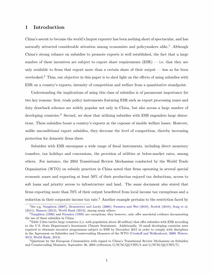
The large number of exporters in China that are eligible to benefit from subsidies with ESR

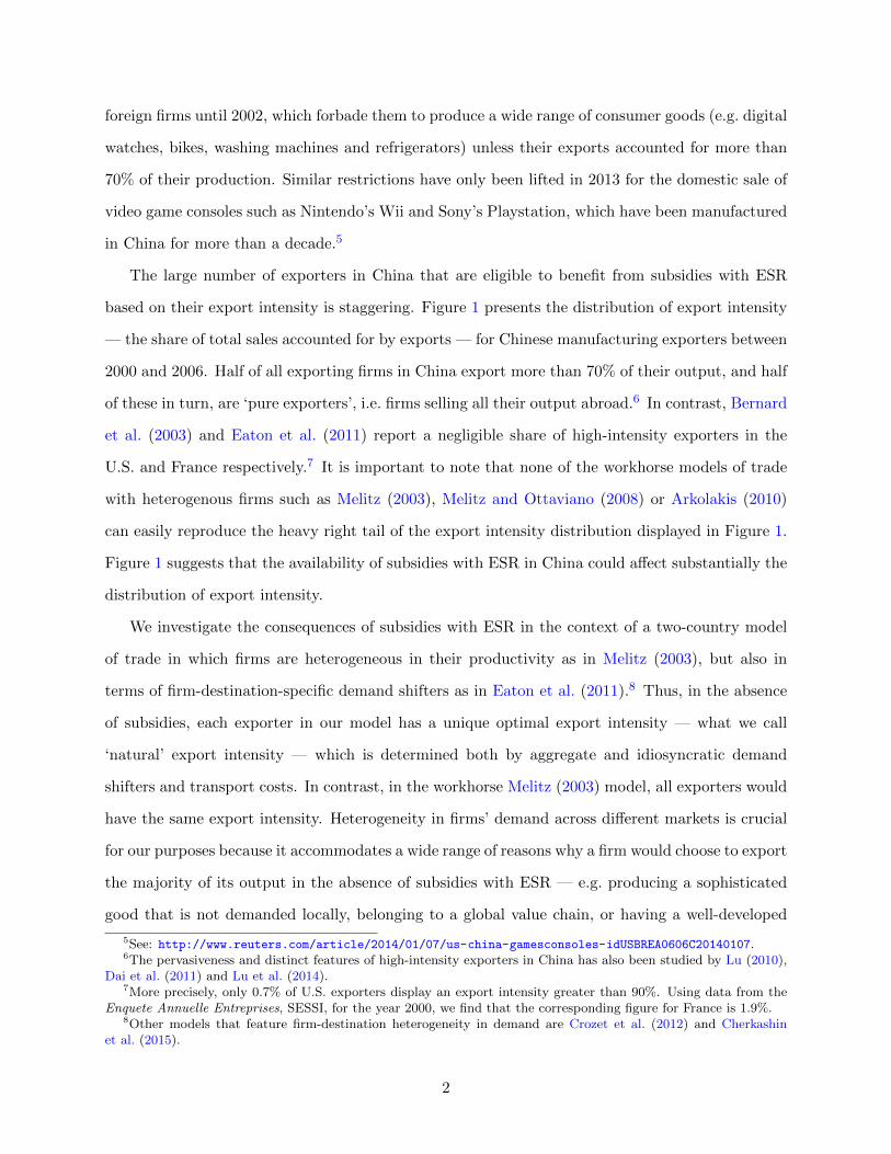
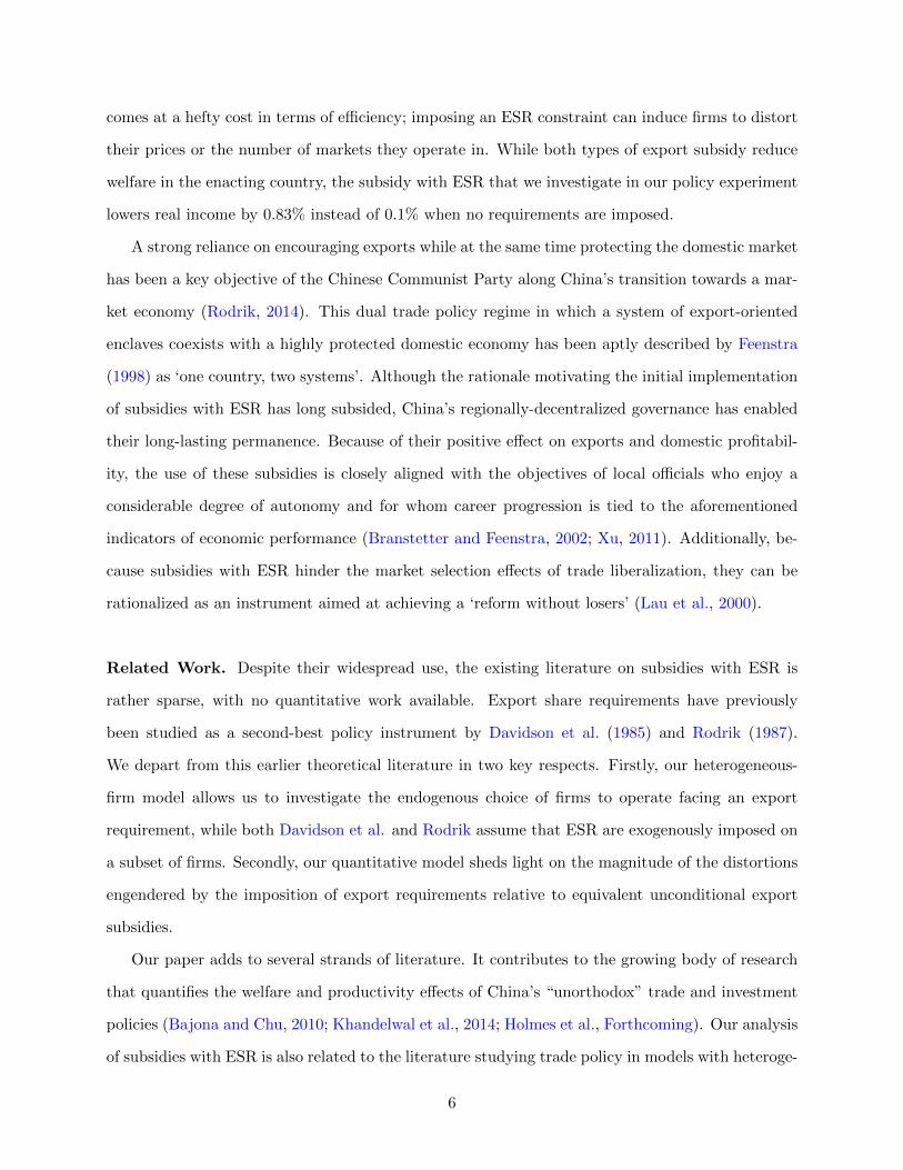
based on their export intensity is staggering. Figure 1 presents the distribution of export intensity

— the share of total sales accounted for by exports — for Chinese manufacturing exporters between

2000 and 2006. Half of all exporting firms in China export more than 70% of their output, and half

of these in turn, are ‘pure exporters’, i.e. firms selling all their output abroad.6 In contrast, Bernard

et al. (2003) and Eaton et al. (2011) report a negligible share of high-intensity exporters in the

U.S. and France respectively.7 It is important to note that none of the workhorse models of trade

with heterogenous firms such as Melitz (2003), Melitz and Ottaviano (2008) or Arkolakis (2010)

can easily reproduce the heavy right tail of the export intensity distribution displayed in Figure 1.

Figure 1 suggests that the availability of subsidies with ESR in China could affect substantially the

distribution of export intensity.

We investigate the consequences of subsidies with ESR in the context of a two-country model

of trade in which firms are heterogeneous in their productivity as in Melitz (2003), but also in

terms of firm-destination-specific demand shifters as in Eaton et al. (2011).8 Thus, in the absence

of subsidies, each exporter in our model has a unique optimal export intensity — what we call

‘natural’ export intensity — which is determined both by aggregate and idiosyncratic demand

shifters and transport costs. In contrast, in the workhorse Melitz (2003) model, all exporters would

have the same export intensity. Heterogeneity in firms’ demand across different markets is crucial

for our purposes because it accommodates a wide range of reasons why a firm would choose to export

the majority of its output in the absence of subsidies with ESR — e.g. producing a sophisticated

good that is not demanded locally, belonging to a global value chain, or having a well-developed

5See: http://www.reuters.com/article/2014/01/07/us-china-gamesconsoles-idUSBREA0606C20140107.6The pervasiveness and distinct features of high-intensity exporters in China has also been studied by Lu (2010),

Dai et al. (2011) and Lu et al. (2014).7More precisely, only 0.7% of U.S. exporters display an export intensity greater than 90%. Using data from the

Enquete Annuelle Entreprises, SESSI, for the year 2000, we find that the corresponding figure for France is 1.9%.8Other models that feature firm-destination heterogeneity in demand are Crozet et al. (2012) and Cherkashin

et al. (2015).

2

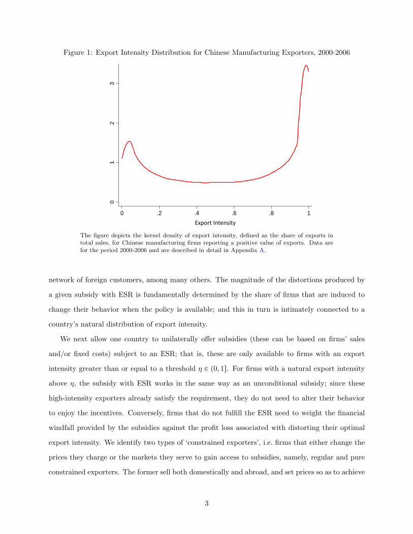
Figure 1: Export Intensity Distribution for Chinese Manufacturing Exporters, 2000-2006

01

23

De

nsity

0 .2 .4 .6 .8 1

Export-IntensityExport Intensity

The figure depicts the kernel density of export intensity, defined as the share of exports intotal sales, for Chinese manufacturing firms reporting a positive value of exports. Data arefor the period 2000-2006 and are described in detail in Appendix A.

network of foreign customers, among many others. The magnitude of the distortions produced by

a given subsidy with ESR is fundamentally determined by the share of firms that are induced to

change their behavior when the policy is available; and this in turn is intimately connected to a

country’s natural distribution of export intensity.

We next allow one country to unilaterally offer subsidies (these can be based on firms’ sales

and/or fixed costs) subject to an ESR; that is, these are only available to firms with an export

intensity greater than or equal to a threshold η P p0, 1s. For firms with a natural export intensity

above η, the subsidy with ESR works in the same way as an unconditional subsidy; since these

high-intensity exporters already satisfy the requirement, they do not need to alter their behavior

to enjoy the incentives. Conversely, firms that do not fulfill the ESR need to weight the financial

windfall provided by the subsidies against the profit loss associated with distorting their optimal

export intensity. We identify two types of ‘constrained exporters’, i.e. firms that either change the

prices they charge or the markets they serve to gain access to subsidies, namely, regular and pure

constrained exporters. The former sell both domestically and abroad, and set prices so as to achieve

3

an export intensity exactly equal to the ESR threshold, while pure constrained exporters choose

instead to only export in order to satisfy the export requirement by saving on domestic fixed costs.

Two key results emerge from our model. Firstly, the introduction of a subsidy with a single

ESR strictly below 1 generates both pure and regular constrained exporters simultaneously —

that is, the mass of firms with an export intensity equal to the ESR and 1 both rise vis-a-vis the

laissez-faire equilibrium. Given that the available incentives in China feature several different ESR

thresholds, ranging from 50 to 100%, our model is consistent with an export intensity distribution

that displays a majority of pure exporters. Secondly, we show that although regular and pure

constrained exporters follow different pricing strategies in response to subsidies, these ultimately

lower the level of competition in the country enacting the policy, increasing the protection of the

least profitable firms. More precisely, regular constrained exporters increase domestic prices and

lower export prices so that their export intensity exactly reaches the ESR threshold. Constrained

pure exporters, on the other hand, do not distort their export price (over and above the direct

reduction in the price due to the sales subsidy), but eliminate their variety altogether from the

domestic consumption basket. Under monopolistic competition both these responses increase the

domestic price index, since this variable is increasing on the average price charged by firms and

decreasing in the number of varieties available for consumption. In contrast, an unconditional

export subsidy lowers the price index in the country providing subsidies. This happens both

because average prices fall — as the least profitable domestic firms exit the market in response to

the expansion of local exporters — and because of tougher import competition, which occurs as

trade partners increase their exports to achieve balanced trade (Demidova and Rodrıguez-Clare,

2009; Felbermayr et al., 2012).

In order to assess the general equilibrium consequences of utilizing subsidies with ESR in our

model, we investigate the effect of one country offering an 8.7% ad-valorem export sales subsidy

subject to a 70% ESR. We choose this specific policy experiment because the magnitude of the

export subsidy is broadly equivalent to one of the best documented fiscal incentives subject to an

ESR in China, the corporate income tax rate discount — from 30 to 10% — offered to foreign-

invested enterprises and Chinese-owned firms located in free trade zones with an export intensity of

at least 70% in place between 1991 and 2008. Since China imposes ESR on a wide range of policy

instruments (which we describe in great detail in Section 2), and since there is extremely limited

4

systematic data on the size and scope of subsidies offered to exporters in China (Lardy, 1992;

Claro, 2006; Girma et al., 2009; Haley and Haley, 2013), carrying out a comprehensive quantitative

evaluation of all subsidies with ESR available in China is beyond the scope of our paper.9 We

instead shed light on how subsidies with ESR operate, by comparing them with the laissez-faire

equilibrium and with an equivalent unconditional subsidy on export sales in terms of the behavior

of price indices (a measure of the intensity of competition), the distribution of export intensity, the

probability of firms’ exit and welfare.

We calibrate our model’s parameters to reflect the share of exporters and the distribution of

export intensity in a hypothetical developing country that does not provide subsidies with ESR,

with the view to approximate a counterfactual scenario in which China does not offer this type of

subsidies. We construct this undistorted distribution of export intensity by combining information

on the use of subsidies with ESR gathered from the U.S. State Department’s Investment Climate

Statements and cross-country firm-level data on firms’ export intensity from the World Bank’s

Enterprise Surveys over the period 2002-2012. As a robustness check, we also use the export

intensity distribution observed in China in 2013, when the corporate income tax deduction subject

to ESR had been phased out.

Our quantitative exercise reveals that given our conjectured natural export intensity distribu-

tion, introducing a subsidy with ESR with the characteristics defined above (which amounts to a

total expenditure in subsidies of 0.19% of GDP in our model) explains 43% of the share of exporters

with an export intensity above 70% observed in China between 2000 and 2006, with approximately

two thirds of the increase in high-intensity exporters accounted for by pure exporters.

Subsidies with ESR produce a substantially greater boost to aggregate exports in the enacting

country than the equivalent unconditional export subsidy (the exports/GDP ratio increases by 6.3%

with the former compared to 2.3% with the latter). At the same time, the intensity of competition

and the probability of firms’ exiting the market are further reduced when subsidies are subject to

export requirements. The combination of these effects implies that the use of subsidies with ESR

can be characterized as ‘protectionism through exporting’. Of course, it follows that such a strategy

9For instance, China did not provide the required subsidy rates or annual amount budgeted for export-relatedsubsidies in either of their notifications to the WTO Committee on Subsidies and Countervailing Measures in 2006and 2011. The notifications were also silent about the extent of subsidies provided at the provincial and local level.See “Request from the United States to China,” October 11, 2011, reference G/SCM/Q2/CHN/42.

5

comes at a hefty cost in terms of efficiency; imposing an ESR constraint can induce firms to distort

their prices or the number of markets they operate in. While both types of export subsidy reduce

welfare in the enacting country, the subsidy with ESR that we investigate in our policy experiment

lowers real income by 0.83% instead of 0.1% when no requirements are imposed.

A strong reliance on encouraging exports while at the same time protecting the domestic market

has been a key objective of the Chinese Communist Party along China’s transition towards a mar-

ket economy (Rodrik, 2014). This dual trade policy regime in which a system of export-oriented

enclaves coexists with a highly protected domestic economy has been aptly described by Feenstra

(1998) as ‘one country, two systems’. Although the rationale motivating the initial implementation

of subsidies with ESR has long subsided, China’s regionally-decentralized governance has enabled

their long-lasting permanence. Because of their positive effect on exports and domestic profitabil-

ity, the use of these subsidies is closely aligned with the objectives of local officials who enjoy a

considerable degree of autonomy and for whom career progression is tied to the aforementioned

indicators of economic performance (Branstetter and Feenstra, 2002; Xu, 2011). Additionally, be-

cause subsidies with ESR hinder the market selection effects of trade liberalization, they can be

rationalized as an instrument aimed at achieving a ‘reform without losers’ (Lau et al., 2000).

Related Work. Despite their widespread use, the existing literature on subsidies with ESR is

rather sparse, with no quantitative work available. Export share requirements have previously

been studied as a second-best policy instrument by Davidson et al. (1985) and Rodrik (1987).

We depart from this earlier theoretical literature in two key respects. Firstly, our heterogeneous-

firm model allows us to investigate the endogenous choice of firms to operate facing an export

requirement, while both Davidson et al. and Rodrik assume that ESR are exogenously imposed on

a subset of firms. Secondly, our quantitative model sheds light on the magnitude of the distortions

engendered by the imposition of export requirements relative to equivalent unconditional export

subsidies.

Our paper adds to several strands of literature. It contributes to the growing body of research

that quantifies the welfare and productivity effects of China’s “unorthodox” trade and investment

policies (Bajona and Chu, 2010; Khandelwal et al., 2014; Holmes et al., Forthcoming). Our analysis

of subsidies with ESR is also related to the literature studying trade policy in models with heteroge-

6

neous firms (Chor, 2009; Demidova and Rodrıguez-Clare, 2009; Davies and Eckel, 2010; Felbermayr

et al., 2012; Cherkashin et al., 2015; Costinot et al., 2015), as well as to the body of work investi-

gating the welfare implications of free trade zones and trade-related investment measures (TRIMs)

(Hamada, 1974; Miyagiwa, 1986; Chao and Yu, 2014; Yucer and Siroen, forthcoming).

The rest of the paper is organized as follows. Section 2 provides an overview of fiscal incentives

featuring export share requirements in China. Section 3 presents our quantitative general equilib-

rium model, and Section 4 spells out our strategy to calibrate the model’s parameters. Section 5

presents the results of our counterfactual experiments. Section 6 concludes.

2 Subsidies with Export Share Requirements in China

In this section we provide a concise overview of policy measures available in China between 2000

and 2006 featuring incentives available to firms conditional on their export intensity exceeding a

stated threshold.

These subsidies were a key innovation introduced in the first wave of opening-up reforms

launched in 1979. Their objective was to facilitate China’s interaction with the rest of the world

without disrupting its socialist economy.10 Despite clearly outgrowing their original purpose, sub-

sidies with ESR have remained ubiquitous in China, even after it joined the WTO in 2001. They

target three types of firms primarily: Chinese-owned firms located in Free Trade Zones (FTZ),

foreign-invested enterprises (FIE) and establishments devoted to export processing activities (PTE).

The online Appendix provides a detailed description of the laws and regulations discussed below. It

is important to note that Free Trade Zones and duty drawback schemes such as China’s processing

trade regime are permitted under WTO agreements. However, if a policy measure is conditioned

on export performance (e.g. setting minimum export targets for firms) such as in the examples

provided below, it would then violate Article 3 of the Agreement on Subsidies and Countervailing

Measures (ASCM) and the Trade-Related Investment Measures (TRIMs) Agreement.11

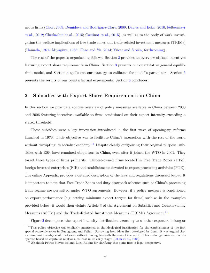
Figure 2 decomposes the export intensity distribution according to whether exporters belong or

10This policy objective was explicitly mentioned in the ideological justification for the establishment of the firstspecial economic zones in Guangdong and Fujian. Borrowing from ideas first developed by Lenin, it was argued thata communist country could not exist without having ties with the rest of the world. This exchange however, had tooperate based on capitalist relations, at least in its early stages (Chan et al., 1986).

11We thank Petros Mavroidis and Luca Rubini for clarifying this point from a legal perspective.

7

not to one of the three types of firms for which subsidies with ESR are more likely to be available.

The contrast between the two groups is again striking. The vast majority of high intensity exporters

are eligible — based on their mode of operation — to benefit from these subsidies; low-intensity

exporters, on the other hand, are more likely to be Chinese-owned firms operating outside a FTZ

and not exporting through the processing regime. See Appendix A for further details.

Figure 2: Export Intensity Distribution according to Eligibility to Receive Subsidies with ESR

01

23

4

Den

sity

0 .2 .4 .6 .8 1Export-Intensity

Firms not eligible for subsidies with Export Share Requirements

Firms eligible for subsidies with Export Share Requirements

• Foreign-Invested Enterprises • Processing Trade Enterprises • Firms located in a Free Trade Zone

• Firms located outside a Free Trade Zone

Export Intensity

The figure depicts the kernel density of export intensity, defined as the share of exports intotal sales, for Chinese manufacturing firms reporting a positive value of exports. Data arefor the period 2000-2006 and are described in detail in Appendix A.

Free Trade Zones. Free Trade Zones are export-oriented enclaves designed to attract both foreign

and domestic investors by providing tax concessions, streamlined regulations, duty-free imports of

materials and equipment used for exporting, among other allowances. For the purposes of the

paper, FTZs include Special Economic Zones, Coastal Development Zones, the Yangtze and Pearl

River Delta Economic Zones as well as smaller industrial parks such as Economic and Technolog-

ical Development Zones, High-Technology Industrial Development Zones and Export Processing

Zones. FTZs vary tremendously in terms of their size, ranging from small enclosed areas to entire

prefecture-cities. Appendix B provides the complete list of prefecture-cities considered.

8

A crucial objective ascribed to FTZs is to be ‘laboratories’ to test market-oriented policies before

their potential implementation in the rest of the economy (Wang, 2013). The Chinese government

initially designated four counties in Guangdong and Fujian provinces as Special Economic Zones in

1979 as one of the components of Deng Xiaoping’s package of economic reforms aimed at reintegrat-

ing China into the world economy. The following two decades witnessed the establishment of a large

number of FTZs in cities located primarily along the coastal regions (see Figure B.1 in Appendix

B), where a vast majority of China’s export-oriented industrial production is concentrated.

China’s corporate income tax regime provides a prime example of the type of incentives available

to firms operating in FTZs which are conditioned on ESR. The statutory corporate income tax rate

prevailing in China between 1991 and 2008 was 30%.12 Chinese-owned firms could reduce their tax

rate to 10% if they were located in an FTZ and exported more than 70% of their output. As a

result of several complaints by the European Union, U.S. and Canada at the WTO, China modified

its corporate income tax legislation substantially in January 2008. Under the new law, a corporate

tax rate of 25% applies both to domestic and foreign companies, and incentives conditioned on ESR

have been scrapped. A five-year transition period was established so that the new tax law became

fully operational in 2013.

Provincial and local managers of FTZs compete fiercely with each other, particularly in seeking

to attract FIEs, and therefore offer a wide array of additional incentives linked to export perfor-

mance such as tax deductions, access to soft loans and priority access to infrastructure and land.

For instance, Standard Chartered Bank (2007) reports that the city of Shenzhen, China’s first spe-

cial economic zone with a total area of 493 km2, offers firms that have paid all their value-added

taxes on inputs and that export the entirety of their production, a 5% sales cash subsidy. The

Shenzhen Special Economic Zone also halves the land use fee charged on certified ‘enterprises-for-

export’. Similarly, most Export Processing Zones specify strict requirements for firms’ domestic

sales allowance – usually 30% of the total volume of sales. The first 15 pilots of this new type

of zone were set up in 2000, and their number has more than tripled over the last decade. Chi-

nese provincial and local governments seem keen to continue experimenting with new strategies to

develop geographically-enclosed areas in which high export intensity firms are encouraged to locate.

12Corporate Income Tax Law of the People’s Republic of China, 16 September 1991, Article 5.

9

Foreign Invested Enterprises. The ‘Twenty-two regulations’, established in 1986 with the

objective of attracting foreign investment, defined an ‘export-oriented’ firm as a manufacturing

enterprise whose export volume accounts for 50% or above of its annual sales.13 FIEs exceeding

this threshold benefitted from preferential land-use policies, easier access to finance and exemptions

from industrial and commercial consolidated tax. Until 2001, being an export-oriented firm was

a requirement for foreign investments in China and FIEs had to specify their share of domestic

sales by contract.14 Firms that did not comply with this requirement faced steep penalties; for

instance, FIEs that did not meet the targets set for export-oriented enterprises within three years

from the day they began production, were required to repay 60% of the tax refunded.15 After

China’s accession to the WTO, the law on Foreign Capital Enterprises revised in October 2000,

lifted the requirement for FIEs to export the majority of their production. Nevertheless, financial

incentives conditional on export intensity have remained in place after 2001.

The first paragraph of the 1991 corporate income tax law stated that “The establishment of

enterprises with foreign investment which export all or the greater part of their production should

be encouraged.”16 Similarly to Chinese-owned firms, FIEs that export more than 70% of their

output lower their corporate income tax rate from 30 to 10%. However, unlike domestically-owned

firms, FIEs are not restricted to be located in FTZ to enjoy this incentive.17

The 1995 regulations entitled “Guiding the Direction of Foreign Investment” also featured

restrictions on local sales for FIEs. According to this law, all foreign investment projects were

classified in one of four categories: encouraged, permitted, restricted and prohibited. However,

restricted projects that exported at least 70% of their total sales were automatically considered

as permitted.18 This regulation is still in place today, despite China substantially revising the list

of restricted products after joining the WTO. The 2002 regulation has introduced a new project

category named “all-for export projects”, which includes any project exporting all its production.

Such projects are treated as encouraged projects automatically and therefore enjoy preferential

13Enforcement of the Provisions of the State Council on Encouraging Foreign Investment, January 1, 1987.14Circular of the Ministry of Foreign Trade and Economic Cooperation on Submission of Import and Export Plans

for Enterprises with Foreign Investment, October 25, 2000.15Corporate Income Tax Law of the People’s Republic of China, 30 June 1991, Article 8.4.4.16Corporate Income Tax Law of the People’s Republic of China’, 9 April 1991, Basic Regulations. 8.1.17‘Corporate Income Tax Law of the People’s Republic of China’, 30 June 1991, Article 8.3.5.18Regulations for Guiding the Direction of Foreign Investment, June 7, 1995, Article 11.

10

treatment,19 e.g. all-for export projects are entitled to a 20% refund of import duty and import

value-added tax.20

The generous tax concessions available to FIEs has driven local Chinese entrepreneurs to en-

gage in what is known as “round-tripping” — i.e. setting up shell companies in Hong Kong, Macau

and Taiwan (HMT), which produce and export goods from China, thereby enjoying tax breaks

— in a massive scale (Prasad and Wei, 2007). HMT-based foreign-invested firms account for ap-

proximately half of all FIEs and more than half of Processing Trade Enterprises operating in China.

Processing Trade Enterprises. China established the legal framework for processing trade in

1979, thus allowing the duty-free importation of inputs and components needed for the production

of goods for export (Naughton, 1996; Fernandes and Tang, 2012). Since the early 1990s, assembling

and processing has consistently accounted for approximately half of China’s export volume. From

a legal standpoint, Processing Trade Enterprises (PTEs) are production enterprises or factories

established by business enterprises but with independent accounting and their own business licence.

Enterprises engaged in processing are required to obtain a production capability certification

as well as a processing trade approval certificate granted by government authorities; they also face

strict controls over their domestic sales. These enterprises are allowed to import inputs duty-free as

long as they are not used for domestic consumption; if any output is sold in the domestic market,

firms must promptly pay the tariffs and VAT on the imported materials. More importantly, they

must obtain approval from both the provincial commerce authorities and customs for an import

licence; failing to do so translates into a penalty ranging from 30 to 100% of the declared value of

the imported materials and parts.21 In practice, firms engaged in export processing either become

fully export-oriented or are forced to set up segregated production facilities to sell domestically

in order to reduce the leakage of tariff-free intermediate goods (Hong Kong Trade Development

Council, 2009; Brandt and Morrow, 2013).

In order to enjoy autonomy regarding domestic sales, a processing trade enterprise has to

19Regulations for Guiding the Direction of Foreign Investment, February 11, 2002.20General Administration of Customs and State Administration of Taxation, 4 September 2002.21Hong Kong Trade Development Council (2003), Guide to Doing Business in China, Chapter on Processing-Trade.

Based on the circular concerning issuance of “Interim Measures on Administration of the Examination and Approvalof Processing Trade” and “Interim Measures on Administration of the Examination and Approval of Domestic Sale ofBonded Materials and Parts Imported for Processing Trade”, Ministry of Foreign Trade and Economic Cooperation(1999, WJMGF. No. 314 and No. 315).

11

change its registration and become a FIE, which requires it to temporarily stop its production

for a customs auditing. The consulting company Li & Fung Group (2012) estimates that this

production disruption takes approximately 9 to 12 months. Furthermore, the transformation from

PTE to FIE involves the work of more than 10 government departments and can potentially result

in a substantial tax repayment.

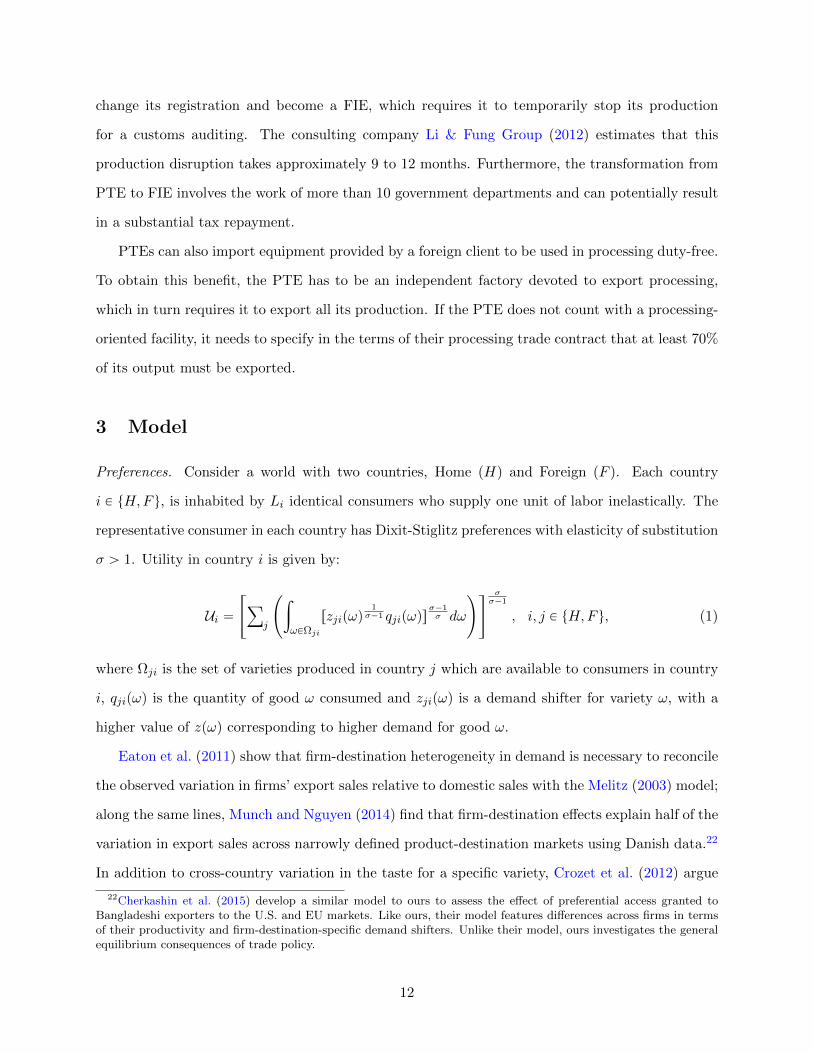
PTEs can also import equipment provided by a foreign client to be used in processing duty-free.

To obtain this benefit, the PTE has to be an independent factory devoted to export processing,

which in turn requires it to export all its production. If the PTE does not count with a processing-

oriented facility, it needs to specify in the terms of their processing trade contract that at least 70%

of its output must be exported.

3 Model

Preferences. Consider a world with two countries, Home (H) and Foreign (F ). Each country

i P tH,F u, is inhabited by Li identical consumers who supply one unit of labor inelastically. The

representative consumer in each country has Dixit-Stiglitz preferences with elasticity of substitution

σ ą 1. Utility in country i is given by:

Ui “

«

ÿ

j

˜

ż

ωPΩji

rzjipωq1

σ´1 qjipωqsσ´1σ dω

¸ffσσ´1

, i, j P tH,F u, (1)

where Ωji is the set of varieties produced in country j which are available to consumers in country

i, qjipωq is the quantity of good ω consumed and zjipωq is a demand shifter for variety ω, with a

higher value of zpωq corresponding to higher demand for good ω.

Eaton et al. (2011) show that firm-destination heterogeneity in demand is necessary to reconcile

the observed variation in firms’ export sales relative to domestic sales with the Melitz (2003) model;

along the same lines, Munch and Nguyen (2014) find that firm-destination effects explain half of the

variation in export sales across narrowly defined product-destination markets using Danish data.22

In addition to cross-country variation in the taste for a specific variety, Crozet et al. (2012) argue

22Cherkashin et al. (2015) develop a similar model to ours to assess the effect of preferential access granted toBangladeshi exporters to the U.S. and EU markets. Like ours, their model features differences across firms in termsof their productivity and firm-destination-specific demand shifters. Unlike their model, ours investigates the generalequilibrium consequences of trade policy.

12

that these demand shifters can also represent a firm’s network of connections with purchasers in

each market. This dimension is particularly important for affiliates of multinational corporations

and firms producing goods specifically customized to individual clients within a global value chain.

These preferences yield the following iso-elastic demand function in country i for variety ω

produced in j:

qjipωq “ Ajipωqpjipωq´σ, with Ajipωq ” EiP

σ´1i zjipωq, (2)

where Ei denotes aggregate expenditure in country i, and Pi, the ideal price index in country i, is

defined as:

Pi “

«

ÿ

j

˜

ż

ωPΩij

zjipωqpjipωq1´σdω

¸ff1

1´σ

, i, j P tH,F u. (3)

Production. Firms in country i incur an initial investment fei to learn their idiosyncratic produc-

tivity, ϕ, and demand shifters pzii, zijq.23 We assume that domestic and export demand shifters are

drawn from the same distribution, Fz and are independent from each other. Productivity is drawn

from a distribution Fϕ, and is also assumed to be independent of demand shifters. With a slight

abuse of notation, let ω ” pϕ, zii, zijq denote a firm’s state vector. Based on their knowledge about

ω, firms first choose whether to stay in or exit the market. If a firm decides to operate, it produces

using a linear technology with labor as the sole input, q “ ϕl; thus, the marginal cost for a firm

with productivity ϕ located in country i is wiϕ, where wi is the wage prevailing in that country.

We assume that firms face a location-specific fixed cost to sell their output in each country

(Eaton et al., 2011) — e.g. a Home-based firm pays fHH when selling domestically and fHF when

it exports to Foreign.24 Moreover, exporters from country i selling in market j incur a transport cost

τij ě 1 on their export sales, whereas there are no transport costs involved in selling domestically,

i.e. τii “ 1, i, j P tH,F u. The combination of location-specific fixed costs with firm-destination-

specific demand shifters means that in the absence of subsidies with ESR there will be three types

of firms operating in equilibrium: firms that sell only domestically (indexed by d), ‘pure’ exporters,

i.e. producers that export all their output (indexed by x), and ‘regular’ exporters, selling their

output both domestically and abroad (indexed by dx).

Heterogeneity in terms of productivity and demand shifters also implies that firms’ choice

23All fixed costs in the model are denominated in units of labor.24Notice that our assumption of location-specific fixed costs implies that these incorporate both production and

“market access” costs.

13

regarding which markets to operate in is not fully characterized by a set of productivity cutoffs

as in the standard Melitz (2003) model. For instance, highly productive firms that experience low

demand draws abroad may not find profitable to export, while the converse can also happen —

some exporters will be less productive than domestic firms. Nevertheless, since regular exporters

face the highest fixed cost (fii ` fij), they are, on average, the most productive type of firm.

As it is well known, all firms set optimal prices that feature a constant mark-up above marginal

cost, which is augmented by the transport cost when a firm exports. Letting k P td, x, dxu index

firms’ mode of operation, profits for firm ω, located in country i and using production mode k, are

given by:

πki pωq “ÿ

j

«

κτ1´σij Aijpωq

ˆ

ϕ

wi

˙σ´1

´ wifij

ff

¨ 1ijpωq, i, j P tH,F u, (4)

where κ ” pσ ´ 1qσ´1σ´σ and 1ijpωq is an indicator function taking the value 1 when firm ω in

country i sells some of its output in market j and zero otherwise.

Conditional on a firm selling a positive quantity abroad, we define an exporter’s ‘natural’ export

intensity, ηki pωq, as the share of its total sales accounted for by exports in the absence of subsidies:

ηki pωq “

$

’

’

&

’

’

%

τ1´σij Aijpωq

Aiipωq`τ1´σij Aijpωq

if k “ dx

1 if k “ x.

(5)

Notice that although a firm’s natural export intensity is independent of its productivity — since the

elasticity of demand and markups in each market are constant — it varies across regular exporters

due to firm-destination-specific demand shifters. Without the latter, not only all regular exporters

would sell the same share of their revenue abroad, but pure exporters would not be able to coexist

alongside domestic firms and regular exporters in equilibrium.

The fact that our model delivers a non-degenerate distribution of firms’ natural export intensity

is critical for our objective of assessing the consequences of subsidies with ESR. Firms choose to

export the majority of their output for a wide variety of reasons besides the availability of subsidies

conditioned on ESR. For instance, they could produce goods for which there is little domestic de-

mand (what Dıaz de Astarloa et al. (2013) call “orphan industries”, e.g. woolen sweater producers

in Bangladesh), or they might operate as links in a global value chain, assembling components into

a new product that is exported in order to continue in the following stage of production. Such

14

naturally-occurring high-intensity exporters certainly benefit from the availability of subsidies with

ESR in our model, but as will become clear below, do not need to distort their behavior to receive

these subsidies.

Subsidies with Export Share Requirements. We now introduce a set of subsidies featuring an

export share requirement (ESR) at Home. Exporters with an export intensity of at least η P p0, 1s,

receive an ad-valorem subsidy sr on their total sales and/or a subsidy sf on their total fixed cost

bill. It is important to note that several of the incentives conditioned on an ESR summarized in

Section 2 involve tax deductions rather than direct cash outlays. Following Bauer et al. (2014), it

is straightforward to show that a sales subsidy for firms operating subject to an ESR is equivalent

to a reduction in the corporate income tax rate on their gross profit (i.e. before incurring fixed

costs).25

Let us now consider the profit maximization problem of a regular exporter at Home facing a

vector of subsidies psr, sf q subject to an ESR with export intensity threshold η:

maxpηHH ,p

ηHF

#

p1`srq“

AHHpωqppηHHq

1´σ `AHF pωqppηHF q

1´σ‰

´

ˆ

wHϕ

˙

“

AHHpωqppηHHq

´σ ` τHFAHF pωqppηHF q

´σ‰

´ p1´ sf qpfHH ` fHF qwH

+

subject to:AHF pωqpp

ηHF q

1´σ

AHHpωqppηHHq

1´σ `AHF pωqppηHF q

1´σě η. (6)

Using the first-order necessary conditions to solve problem (6), we can readily establish that,

Lemma 1 If ηdxH pωq ă η, then the ESR constraint is binding.

Proof. See Appendix C.

In other words, a regular exporter with natural export intensity below the ESR threshold seeking

to receive these subsidies, would choose its domestic and export prices so that its export intensity

is exactly equal to η. We can now use Lemma 1 to solve problem (6), and characterize the optimal

prices charged by exporters benefiting from subsidies with ESR. The solution involves two cases.

First, consider a firm for which ηdxH pωq ă η — that is, a firm which finds the ESR constraint binding.

25If the corporate income tax was levied on net profits (including fixed costs), then a tax deduction subject to anexport requirement would be equivalent to a combination of a sales subsidy and a fixed cost tax for firms operatingsubject to an ESR. We discuss this in more detail in Section 5.

15

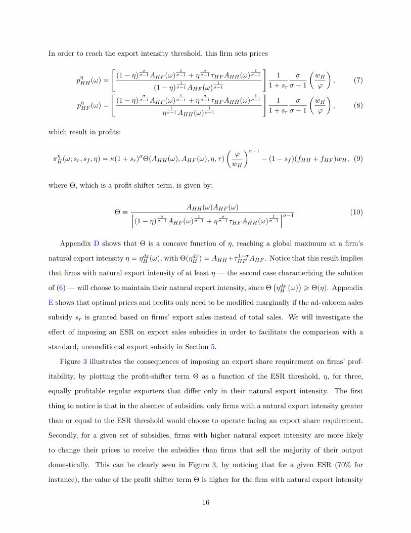
In order to reach the export intensity threshold, this firm sets prices

pηHHpωq “

«

p1´ ηqσσ´1AHF pωq

1σ´1 ` η

σσ´1 τHFAHHpωq

1σ´1

p1´ ηq1

σ´1AHF pωq1

σ´1

ff

1

1` sr

σ

σ ´ 1

ˆ

wHϕ

˙

, (7)

pηHF pωq “

«

p1´ ηqσσ´1AHF pωq

1σ´1 ` η

σσ´1 τHFAHHpωq

1σ´1

η1

σ´1AHHpωq1

σ´1

ff

1

1` sr

σ

σ ´ 1

ˆ

wHϕ

˙

, (8)

which result in profits:

πηHpω; sr, sf , ηq “ κp1` srqσΘpAHHpωq, AHF pωq, η, τq

ˆ

ϕ

wH

˙σ´1

´ p1´ sf qpfHH ` fHF qwH , (9)

where Θ, which is a profit-shifter term, is given by:

Θ ”AHHpωqAHF pωq

”

p1´ ηqσσ´1AHF pωq

1σ´1 ` η

σσ´1 τHFAHHpωq

1σ´1

ıσ´1 . (10)

Appendix D shows that Θ is a concave function of η, reaching a global maximum at a firm’s

natural export intensity η “ ηdxH pωq, with ΘpηdxH q “ AHH`τ1´σHF AHF . Notice that this result implies

that firms with natural export intensity of at least η — the second case characterizing the solution

of (6) — will choose to maintain their natural export intensity, since Θ`

ηdxH pωq˘

ě Θpηq. Appendix

E shows that optimal prices and profits only need to be modified marginally if the ad-valorem sales

subsidy sr is granted based on firms’ export sales instead of total sales. We will investigate the

effect of imposing an ESR on export sales subsidies in order to facilitate the comparison with a

standard, unconditional export subsidy in Section 5.

Figure 3 illustrates the consequences of imposing an export share requirement on firms’ prof-

itability, by plotting the profit-shifter term Θ as a function of the ESR threshold, η, for three,

equally profitable regular exporters that differ only in their natural export intensity. The first

thing to notice is that in the absence of subsidies, only firms with a natural export intensity greater

than or equal to the ESR threshold would choose to operate facing an export share requirement.

Secondly, for a given set of subsidies, firms with higher natural export intensity are more likely

to change their prices to receive the subsidies than firms that sell the majority of their output

domestically. This can be clearly seen in Figure 3, by noticing that for a given ESR (70% for

instance), the value of the profit shifter term Θ is higher for the firm with natural export intensity

16

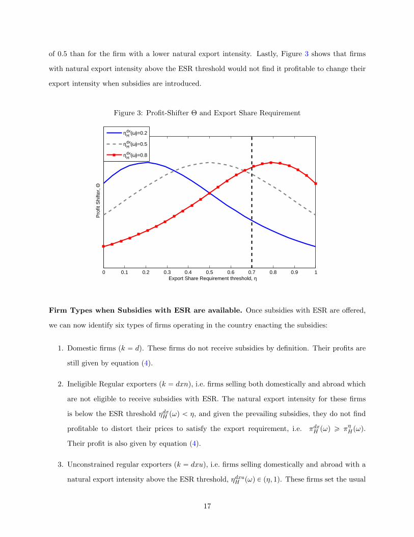
of 0.5 than for the firm with a lower natural export intensity. Lastly, Figure 3 shows that firms

with natural export intensity above the ESR threshold would not find it profitable to change their

export intensity when subsidies are introduced.

Figure 3: Profit-Shifter Θ and Export Share Requirement

0 0.1 0.2 0.3 0.4 0.5 0.6 0.7 0.8 0.9 1Export Share Requirement threshold, η

Pro

fit S

hifte

r, Θ

ηdx

H (ω)=0.2

ηdxH (ω)=0.5

ηdxH (ω)=0.8

Firm Types when Subsidies with ESR are available. Once subsidies with ESR are offered,

we can now identify six types of firms operating in the country enacting the subsidies:

1. Domestic firms (k “ d). These firms do not receive subsidies by definition. Their profits are

still given by equation p4q.

2. Ineligible Regular exporters (k “ dxn), i.e. firms selling both domestically and abroad which

are not eligible to receive subsidies with ESR. The natural export intensity for these firms

is below the ESR threshold ηdxH pωq ă η, and given the prevailing subsidies, they do not find

profitable to distort their prices to satisfy the export requirement, i.e. πdxH pωq ě πηHpωq.

Their profit is also given by equation p4q.

3. Unconstrained regular exporters (k “ dxu), i.e. firms selling domestically and abroad with a

natural export intensity above the ESR threshold, ηdxuH pωq P pη, 1q. These firms set the usual

17

constant markup above marginal cost under laissez-faire but lower their prices in proportion

to the magnitude of the subsidy on sales, sr. They set domestic and export prices pdxuHH “

11`sr

σσ´1

wHϕ and pdxuHF “ τHF p

dxuHH respectively, and realize profits:

πdxuH pω; sr, sf , ηq “ κp1` srqσrAHHpωq` τ

1´σHF AHF pωqs

ˆ

ϕ

wH

˙σ´1

´p1´ sf qpfHH ` fHF qwH .

(11)

They maintain their natural export intensity after the introduction of the subsidies.

4. Pure exporters (k “ xu) that would only serve the export market even in the absence of

subsidies. These firms export all their output and therefore meet the export share requirement

by definition. Subsidies with ESR are equivalent to unconditional subsidies for them. It is

straightforward to show that pure exporters lower their export prices, pxuHF “1

1`srσσ´1

τHFwHϕ

in response to the sales subsidy, and achieve profits

πxuH pωq “ κp1` srqστ1´σHF AHF pωq

ˆ

ϕ

wH

˙σ´1

´ p1´ sf qfHFwH , (12)

which are higher than in the absence of subsidies with ESR.

5. Constrained regular exporters (k “ dxc). These firms, which would have a natural export

intensity below the ESR under laissez-faire, choose to sell domestically and abroad and set

prices in order to achieve an export intensity exactly equal to η. For these firms, the gain due

to the subsidies exceeds the profit loss produced by the distortion of their prices.

6. Constrained pure exporters (k “ xc). These firms would not have chosen to operate as pure

exporters had the subsidies with ESR not being in place. These firms set the same export

prices and obtain the same profits as unconstrained pure exporters.

Firms choose their type in order to maximize profits with full information of both their pro-

ductivity and demand shifters. Table 1 summarizes the different firm types that can potentially

coexist in the country offering subsidies with ESR.

Differences between Pure and Regular Constrained Exporters. Firstly, we want to em-

phasize the fact that a single ESR threshold η P p0, 1q generates both pure exporters and regular

18

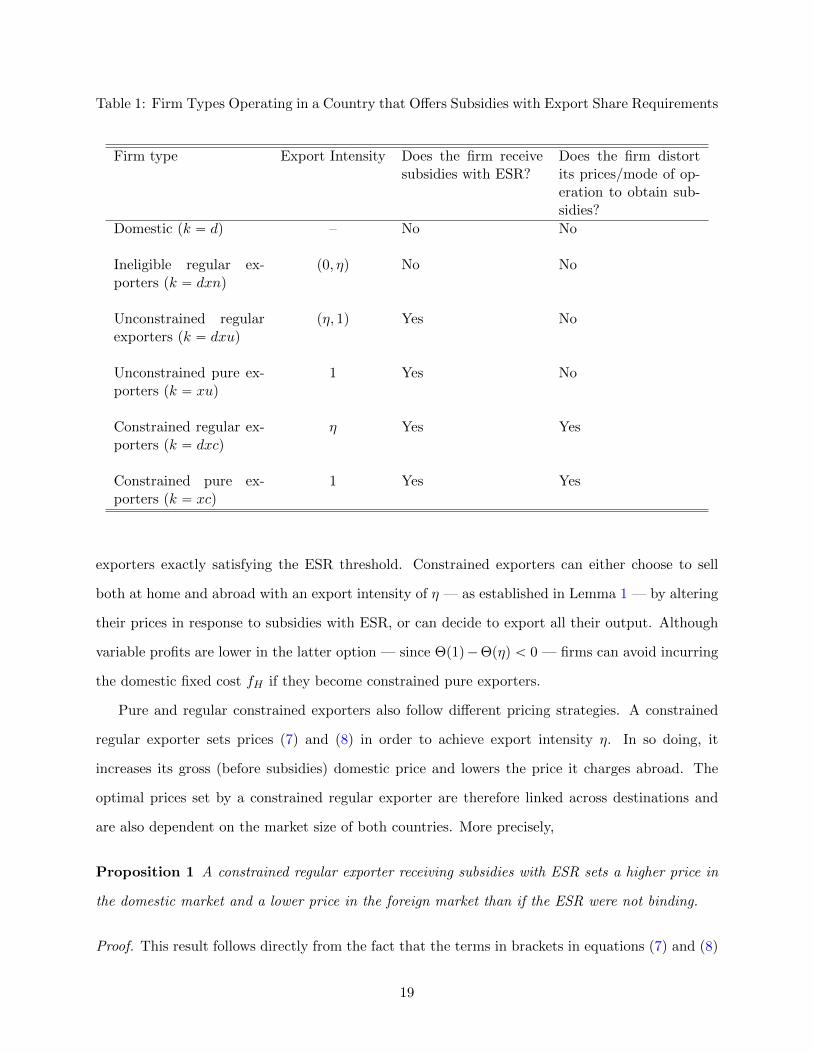
Table 1: Firm Types Operating in a Country that Offers Subsidies with Export Share Requirements

Firm type Export Intensity Does the firm receivesubsidies with ESR?

Does the firm distortits prices/mode of op-eration to obtain sub-sidies?

Domestic (k “ d) – No No

Ineligible regular ex-porters (k “ dxn)

p0, ηq No No

Unconstrained regularexporters (k “ dxu)

pη, 1q Yes No

Unconstrained pure ex-porters (k “ xu)

1 Yes No

Constrained regular ex-porters (k “ dxc)

η Yes Yes

Constrained pure ex-porters (k “ xc)

1 Yes Yes

exporters exactly satisfying the ESR threshold. Constrained exporters can either choose to sell

both at home and abroad with an export intensity of η — as established in Lemma 1 — by altering

their prices in response to subsidies with ESR, or can decide to export all their output. Although

variable profits are lower in the latter option — since Θp1q´Θpηq ă 0 — firms can avoid incurring

the domestic fixed cost fH if they become constrained pure exporters.

Pure and regular constrained exporters also follow different pricing strategies. A constrained

regular exporter sets prices (7) and (8) in order to achieve export intensity η. In so doing, it

increases its gross (before subsidies) domestic price and lowers the price it charges abroad. The

optimal prices set by a constrained regular exporter are therefore linked across destinations and

are also dependent on the market size of both countries. More precisely,

Proposition 1 A constrained regular exporter receiving subsidies with ESR sets a higher price in

the domestic market and a lower price in the foreign market than if the ESR were not binding.

Proof. This result follows directly from the fact that the terms in brackets in equations (7) and (8)

19

are respectively greater than 1 and lower than τHF when η P`

ηdxH pωq, 1˘

.

Thus, a binding ESR constraint induces exporters to reduce domestic sales and to increase the

output exported in order to achieve export intensity η. Conversely, a constrained firm that decides

to give up its domestic sales does not distort the markup it charges on export sales beyond the

direct effect of the sales subsidy. However, if the mass of constrained pure exporters increases, the

number of varieties available to home consumers falls, thereby increasing the domestic price index

and lowering the level of competition domestically. Thus, as the level of subsidies subject to an

ESR increase and the share of constrained exporters rises accordingly, the level of competition in

the country enacting the subsidies falls and protection for the least profitable firms heightens. This

result follows from the fact that the price index defined in (3) is increasing in the average price

charged by firms, but decreasing in the number of varieties available for consumption. Solving for

the general equilibrium in our model when one country makes use of subsidies with ESR allows us

to provide a magnitude of the distortions generated by this policy.

General Equilibrium. We now describe the conditions that characterize the general equilibrium

in our model. As noted above, we assume that only Home offers subsidies with ESR — this is the

only difference between the two countries in our benchmark. We assume that the Home government

runs a balanced budget and finances subsidies by imposing a lump-sum tax on households.

Choosing labor at Home as the numeraire (wH “ 1), and given a vector of subsidies psr, sf q,

equilibrium in the model is characterized by a vector of seven endogenous variables,

!

MH ,MF , PH , PF , EH , EF , wF

)

,

all of which have been defined above, with the exception of MH and MF , which denote the mass

of operating firms at Home and Foreign respectively. Equilibrium is such that in each country,

(i) the labor market clears,

(ii) expected profits of entering the market exactly cover entry costs,

(iii) Total expenditure in country i is given by: Ei “ wiLi ´ Ti, where Ti is the aggregate tax

revenue used to finance export subsidies,

20

and international trade is balanced. Appendix F describes the algorithm used to solve the model

numerically, and spells out in detail the market-clearing equations listed above.

4 Calibration

This section describes the procedure used to assign values to the endowments, preferences and

technology parameters of our model economy. We calibrate our model so as to reproduce salient

features of the distribution of export intensity of a developing country that does not provide sub-

sidies with ESR.

Natural Export Intensity Distribution. As we discussed in Section 3, the consequences of

subsidies conditioned on ESR depend crucially on the natural distribution of export intensity that

would have prevailed in a country had such subsidies not been available. For instance, relatively

few firms would choose to change their mode of operation — to become either constrained pure or

regular exporters — in response to a given subsidy and ESR threshold combination if the natural

export intensity distribution was highly skewed to the left. Conversely, in a country where high-

intensity exporters are more prevalent, fewer firms would choose to distort their prices to receive

the subsidy. However, it is possible that the aggregate expenditure in subsidies would be higher

in the latter scenario — potentially making a given subsidy more distortive — because there are

more firms eligible to receive subsidies.

We utilize cross-country firm-level data drawn from the World Bank’s Enterprise Surveys

(WBES) for the years 2002-2012 to construct a natural export intensity distribution that is not

distorted by subsidies with ESR and that will serve as the benchmark for our quantitative exer-

cise. Our sample consists of manufacturing exporters operating in the twenty largest developing

and transition countries in terms of population (i.e. those with at least 30 million inhabitants),

for which there are at least 100 exporters available in WBES. Since our objective is to infer the

counterfactual distribution that would have prevailed in China in the absence of subsidies with

ESR, we therefore choose to use relatively large countries to construct our natural export intensity

distribution; moreover, Defever and Riano (2015b) find that the share of high-intensity exporters

observed in a country is crucially influenced by its size.

21

We collect information on whether a country provides or not subsidies with ESR from the

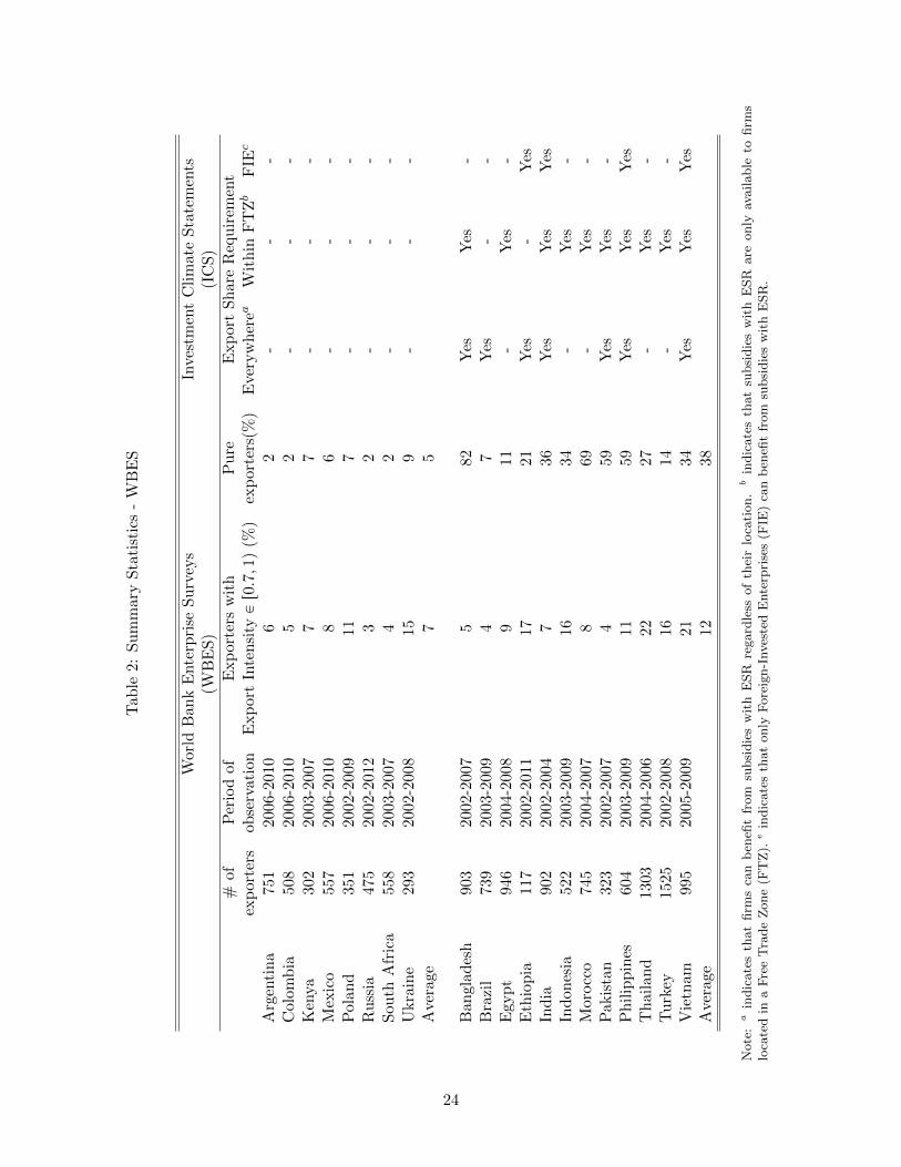
Investment Climate Statements produced by the U.S. State Department.26 Table 2 presents the

countries included in our sample, as well as the number of exporters and the share of high-intensity

(i.e. those with export intensity above 70%) exporters operating in each country. The last three

columns of the table indicate whether subsidies with ESR are also conditioned on a firm’s location

or ownership status. The column “Everywhere” indicates that any firm can benefit from subsidies

with ESR regardless of their location; “within a FTZ” indicates that the subsides are only available

to firms located in a Free Trade Zone, and the last column “FIE” indicates that only Foreign-

Invested Enterprises are eligible. Since countries often implement several policy measures subject

to ESR at the same time, these categories are not mutually exclusive.

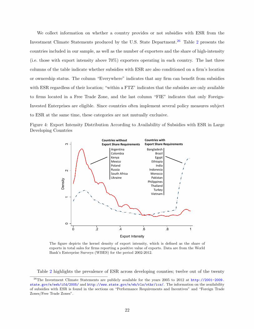
Figure 4: Export Intensity Distribution According to Availability of Subsidies with ESR in LargeDeveloping Countries

Argentina Colombia Kenya Mexico Poland Russia South Africa Ukraine

Countries without Export Share Requirements

Countries with Export Share Requirements

Bangladesh Brazil Egypt

Ethiopia India

Indonesia Morocco Pakistan

Philippines Thailand

Turkey Vietnam

The figure depicts the kernel density of export intensity, which is defined as the share ofexports in total sales for firms reporting a positive value of exports. Data are from the WorldBank’s Enterprise Surveys (WBES) for the period 2002-2012.

Table 2 highlights the prevalence of ESR across developing counties; twelve out of the twenty

26The Investment Climate Statements are publicly available for the years 2005 to 2012 at http://2001-2009.

state.gov/e/eeb/ifd/2005/ and http://www.state.gov/e/eb/rls/othr/ics/. The information on the availabilityof subsidies with ESR is found in the sections on “Performance Requirements and Incentives” and “Foreign TradeZones/Free Trade Zones”.

22

countries in our sample offer incentives to firms conditioned on fulfilling an explicit export share

requirement. Figure 4 presents the distribution of export intensity for exporters based on the

availability of subsidies with ESR. Once again, the difference between the two distributions is

remarkable — on average half of exporters in countries offering subsidies with ESR export 70%

or more of their output, while only 12% do so in countries that do not offer these subsidies (the

distribution for the latter group of firms closely resembles the one for domestically-owned Chinese

firms located outside FTZ presented in Figure 2). This marked contrast provides further suggestive

evidence regarding the role of subsidies with ESR in distorting the distribution of export intensity.

Thus, we will use the export intensity distribution for exporters located in non-ESR countries — the

solid line in Figure 4 — as the natural export intensity distribution when calibrating our model. It

is important to note that when computing both the densities in Figure 4 and the moments targeted

in the calibration, each firm-level export intensity observation is weighted so that each country

receives an equal weight. This ensures that the distributions are not driven by outliers, or sample

size and population differences across countries.

Assigned Parameters. In order to calibrate our model, we assume that both Home and Foreign

countries are identical in terms of their labour endowments and model parameters. Thus, firms in

both countries draw productivity and destination-specific demand shifters from the same distribu-

tions. This assumption also implies that the fixed costs of entry and operation in each market are

such that fei “ fej “ fe, fii “ fjj “ fd and fij “ fji “ fx for i, j P tH,F u and i ‰ j. Since scaling

up or down all fixed costs by the same amount does not affect the aggregate variables of interest

— just as in Melitz and Redding (2015) — we normalize the domestic fixed cost fd to 1.

We assume that both Home and Foreign have the same population, so that L “ 1. If one

considers Home (i.e. the country enacting subsidies with ESR) to be China, then this assumption

implies that Foreign in our model corresponds to a country with the combined population of the

U.S., Canada and the EU (Khandelwal et al., 2014).

We set the elasticity of substitution, σ, equal to 3, based on Broda and Weinstein (2006).27

27We have also experimented with an elasticity of substitution of 3.5, which is the average value of the medianimport demand elasticities at the SITC 3-digit level for Argentina, Colombia, Mexico and Poland, the four countriesbelonging to our undistorted benchmark for which Broda et al. (2006) have estimates available, and which is in turnvery close to China’s estimate of 3.42, and our results remain robust. Table H.1 presents further robustness checksin which we perturb our calibrated parameters one at a time.

23

Tab

le2:

Su

mm

ary

Sta

tist

ics

-W

BE

S

Wor

ldB

ank

Ente

rpri

seS

urv

eys

Inve

stm

ent

Cli

mat

eS

tate

men

ts(W

BE

S)

(IC

S)

#of

Per

iod

ofE

xp

orte

rsw

ith

Pu

reE

xp

ort

Sh

are

Req

uir

emen

tex

por

ters

obse

rvat

ion

Exp

ort

Inte

nsi

tyPr0.7,1q

(%)

exp

orte

rsp%q

Eve

ryw

her

eaW

ith

inF

TZb

FIE

c

Arg

enti

na

751

2006-

2010

62

--

-C

olom

bia

508

200

6-2

010

52

--

-K

enya

302

200

3-2

007

77

--

-M

exic

o55

7200

6-2

010

86

--

-P

olan

d351

2002

-2009

117

--

-R

uss

ia475

2002

-2012

32

--

-S

ou

thA

fric

a558

2003-

2007

42

--

-U

kra

ine

293

200

2-2

008

159

--

-A

vera

ge7

5

Ban

glad

esh

903

2002

-2007

582

Yes

Yes

-B

razi

l73

92003

-2009

47

Yes

--

Egyp

t94

620

04-

200

89

11-

Yes

-E

thio

pia

117

2002-

2011

1721

Yes

-Y

esIn

dia

902

2002

-2004

736

Yes

Yes

Yes

Ind

on

esia

522

200

3-2

009

1634

-Y

es-

Mor

occ

o745

2004

-2007

869

-Y

es-

Pak

ista

n323

2002-

2007

459

Yes

Yes

-P

hil

ipp

ines

604

2003

-2009

1159

Yes

Yes

Yes

Th

ail

an

d130

3200

4-2

006

2227

-Y

es-

Tu

rkey

1525

2002-2

008

1614

-Y

es-

Vie

tnam

995

2005

-2009

2134

Yes

Yes

Yes

Ave

rage

1238

Note

:a

indic

ate

sth

at

firm

sca

nb

enefi

tfr

om

subsi

die

sw

ith

ESR

regard

less

of

thei

rlo

cati

on.b

indic

ate

sth

at

subsi

die

sw

ith

ESR

are

only

available

tofirm

slo

cate

din

aF

ree

Tra

de

Zone

(FT

Z).e

indic

ate

sth

at

only

Fore

ign-I

nves

ted

Ente

rpri

ses

(FIE

)ca

nb

enefi

tfr

om

subsi

die

sw

ith

ESR

.

24

Firms in both countries draw their productivity realizations from a Pareto distribution with lower

bound 1 and shape parameter a. Following Helpman et al. (2004), we estimate a ´ pσ ´ 1q by

regressing the logarithm of a firm’s employment ranking on the logarithm of its employment level

using data from our sample of countries not offering subsidies with ESR. The estimated coefficient

of 0.713 implies a value of a “ 3.213, given our choice of σ.

Similarly to other model parameters, the iceberg transport cost incurred is assumed to be the

same for both countries, i.e. τHF “ τFH “ τ . In models that do not feature firm-destination-

specific demand shifters (e.g. Melitz and Redding, 2015), transport costs are usually calibrated to

match a country’s mean export intensity.28 In our model, however, changes in transport costs or

in the mean of demand shifters both affect the export intensity distribution. The only difference

between transport costs and the mean of export demand shifters, is that the former affects the

price of exports relative to the domestic market price while the latter does not. Since we do not

have information on prices that allows us to separately identify the two parameters, we set τ equal

to 1.7 following Anderson and van Wincoop (2004).

Calibrated Parameters. There are 5 parameters that remain to be calibrated, which we choose

so as to minimize the distance between a number of moments in the model and in the data. These

are the sunk cost of entry, fe, the fixed cost of exporting, fx, and the parameters governing

the distribution of firm-specific domestic and export demand shifters. We assume that the latter

are both drawn from lognormal distributions with parameters pµd, σ2dq and pµx, σ

2xq, which denote

the mean and variance of the underlying normal distribution for each demand shifter. We set

µd “ ´0.5σ2d so that domestic demand shifters have a mean of 1. The moments we target are the

share of exporting firms (37.42%) and the 10th, 50th, 75th and 90th percentiles of the distribution

of export intensity in countries that do not provide subsidies with ESR.

Table 3 summarizes the parameters used to solve the model. Our model fits the distribution of

export intensity quite well, as Figure 5 shows, although we overstate the share of pure exporters,

which is not a targeted moment. The model implies an employment size premium for exporters

vis-a-vis domestic firms of 1.17 log points (relative to 1.31 in our sample of non-ESR countries),

28Recall that in the Melitz (2003) model with identical countries, all exporters have the same export intensity,τ1´σ

p1` τ1´σq.

25

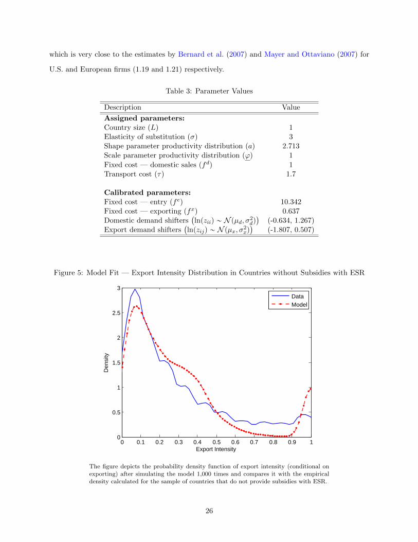
which is very close to the estimates by Bernard et al. (2007) and Mayer and Ottaviano (2007) for

U.S. and European firms (1.19 and 1.21) respectively.

Table 3: Parameter Values

Description Value

Assigned parameters:Country size (L) 1Elasticity of substitution (σ) 3Shape parameter productivity distribution (a) 2.713Scale parameter productivity distribution (ϕ) 1

Fixed cost — domestic sales (fd) 1Transport cost (τ) 1.7

Calibrated parameters:Fixed cost — entry (fe) 10.342Fixed cost — exporting (fx) 0.637Domestic demand shifters

`

lnpziiq „ N pµd, σ2dq˘

(-0.634, 1.267)Export demand shifters

`

lnpzijq „ N pµx, σ2xq˘

(-1.807, 0.507)

Figure 5: Model Fit — Export Intensity Distribution in Countries without Subsidies with ESR

0 0.1 0.2 0.3 0.4 0.5 0.6 0.7 0.8 0.9 10

0.5

1

1.5

2

2.5

3

Export Intensity

Den

sity

DataModel

The figure depicts the probability density function of export intensity (conditional onexporting) after simulating the model 1,000 times and compares it with the empiricaldensity calculated for the sample of countries that do not provide subsidies with ESR.

26

5 The Effect of Subsidies with Export Share Requirements

We now investigate the effect of introducing subsidies with export share requirements on prices,

the distribution of export intensity, the intensity of competition and welfare in our model economy.

As we have documented in Section 2, there is a large number of policy measures that provide

subsidies subject to ESR in China. Besides differences in the underlying policy (e.g. tax holidays,

access to soft loans, subsidized utilities), these incentives also differ in terms of their specific ESR

thresholds (in some cases these can even be firm-specific), additional location and/or ownership

requirements and administrative scope (i.e. the available incentives vary at the national, provincial

and prefecture-city level). Thus, carrying out a comprehensive quantitative assessment of the

consequences of subsidies with ESR in China is beyond the scope of this paper.

We instead choose to pursue a more modest objective. In order to investigate the effect of

subsidies with ESR we focus on the corporate income tax deduction available to firm with an export

intensity above 70% to anchor our quantitative exercise. To be precise, FIEs and Chinese-owned

firms located in FTZ satisfying the aforementioned ESR enjoyed a reduction of their corporate

income tax rate from 30 to 10% between 1991 and 2008. This policy is appealing because is set

at the national level and has a broad coverage (Figure B.1 in Appendix B shows that the FTZ

location requirement is not unduly restrictive).

As it is well known, the gross profit of a firm under monopolistic competition facing iso-elastic

demand is proportional to its revenue. Hence, profits after corporate income tax, t, are given by

πpωq “ p1´tq rrpωqσ ´ f s, where rpωq denotes a firm’s total sales revenue and f its total fixed cost

bill. Thus, reducing the corporate income tax rate faced by firms satisfying a 70% ESR from 30%

to 10% implies a 28.6% (=0.9/0.7) increase in both gross profits and the fixed cost bill compared

to firms that do not comply with the export requirement. Given the vector of sales and fixed

cost subsidies analyzed in the previous section, the aforementioned corporate income tax deduction

would be equivalent to an ad-valorem sales subsidy sr “ 8.7% (since this subsidy increases gross

profits by a factor p1 ` srqσ, it follows that 0.087 « 1.28613 ´ 1, given our choice of σ “ 3) and

a fixed cost tax, sf “ ´28.6% vis-a-vis firms that do not fulfill the requirement. Notice, however,

that if the corporate income tax was levied on gross profits, this would entail setting the fixed cost

subsidy equal to zero.

27

In order to elucidate how subsidies with ESR operate, we assume that the sales subsidy is

granted based on a firm’s export sales rather than on its total sales, while also abstracting from

the fixed cost subsidy.29 Doing so, allows us to compare the subsidy subject to an ESR with an

equivalent (in the sense of the total expenditure on subsidies being the same in both scenarios)

unconditional export subsidy and laissez-faire. Thus, in our benchmark experiment, we assume

that the government at Home offers an 8.7% ad-valorem subsidy to export sales for firms with an

export intensity of at least 70%.

We first investigate how the use of a subsidy with ESR affects the mode of operation choice for

firms at Home. As Figure 5 shows, 10.2% of exporters, the majority of which are pure exporters,

have a natural export intensity above 70%. Following the introduction of the export sales subsidy

with ESR, the share of exporters with an export intensity above the ESR threshold doubles. To put

this figure in context, the export sales subsidy subject to an ESR that we consider in our experiment

would account for 43% of the exporters with an export intensity of 70% or above observed in China

between 2000 and 2006. Notably, the greatest change takes place at the upper bound of the export

intensity distribution, as the share of pure exporters increases by 6.88 percentage points, while

4.3% of exporters choose to operate as constrained regular exporters, achieving exactly a 70%

export intensity. As we noted in Section 3 above, more firms choose to operate as constrained

pure exporters instead of at the ESR threshold when their domestic demand is small compared

to that faced abroad and also when the fixed cost of operating domestically is high relative to

that associated with exporting. Nevertheless, our quantitative exercise is likely to overestimate

the mass point in the distribution of export intensity at 70%, since we are not taking into account

the potential administrative burden that firms subject to ESR face when selling domestically. For

instance, firms need to demonstrate that they effectively sell less than 30% of their output on the

domestic market, for instance by using different production establishments or separated production

lines for their export and domestic sales production; pure exporters, on the other hand, are likely

to be less affected by these.

Firms that go on to operate facing an ESR while selling both at Home and Foreign have a

mean natural export intensity of 54%, which is approximately twice as large as the overall average

29Offering an 8.7% total sales subsidy in addition to a 28.6% fixed cost tax as discussed above yields similarqualitative results as those produced by our benchmark policy experiment discussed below. From a quantitativestandpoint, the effect of the policy on aggregate exports, the intensity of competition and welfare is less pronounced.

28

natural export intensity under laissez-faire. This follows because the distortion in profits caused

by the ESR is lower the closer a firm’s natural export intensity is to the ESR threshold, and is

therefore more easily compensated by a given subsidy. Maintaining the natural export intensity

constant, we find that constrained regular exporters are 35% more productive than the average

Home exporter when there are no subsidies in place, while constrained pure exporters are 25% less

productive than the same reference group. Thus, we can see that the selection pattern induced by

the ESR constraint is heterogeneous with respect to firms’ productivity. On the one hand, firms

that operate at the ESR threshold are sufficiently productive to incur the fixed costs involved in

selling at home and abroad. On the other hand, relatively less productive firms prefer instead to

become constrained pure exporters, since by doing so they gain access to the export subsidies and

economize the fixed cost required to selling domestically.

Table 4 presents the impact of export subsidies, both unconditional and with ESR, vis-a-vis

laissez faire on several equilibrium variables such as exports/GDP, price indices, the unconditional

probability of firm exit and welfare. In this exercise, we contrast the 8.7% subsidy on export sales

granted to firms with an export intensity of at least 70% with a 2.9% ad-valorem export sales

subsidy made available to all exporters regardless of their export intensity, both of which result in

Home’s aggregate expenditure on export subsidies being 0.19% of GDP.

We begin by noting that subsidies with ESR share several key features with unconditional export

subsidies. Both policy instruments increase aggregate exports in the enacting country, deteriorate

its terms-of-trade, reduce welfare and produce qualitatively similar effects on its trade partners.

More precisely, the provision of export subsidies at Home lowers the price of (at least some of)

Home’s export varieties, intensifying import competition in Foreign and lowering the price index

there. Restoring trade balance, in turn, requires Foreign’s wage to fall so that firms operating there

become more competitive, and ultimately, increase their exports to Home. The fall in the price

index in Foreign more than compensates the fall in its nominal wage, and thus welfare (i.e. real

income) in Foreign increases at the expense of Home (Felbermayr et al., 2012).30

Unlike unconditional export subsidies, however, Table 4 shows that subsidies with ESR increase

30Demidova and Rodrıguez-Clare (2009) also find that unconditional export subsidies lower Home’s terms-of-tradeand welfare. Since they model a small economy, however, Home’s export subsidies do not affect price indices orwelfare in the rest of the world.

29

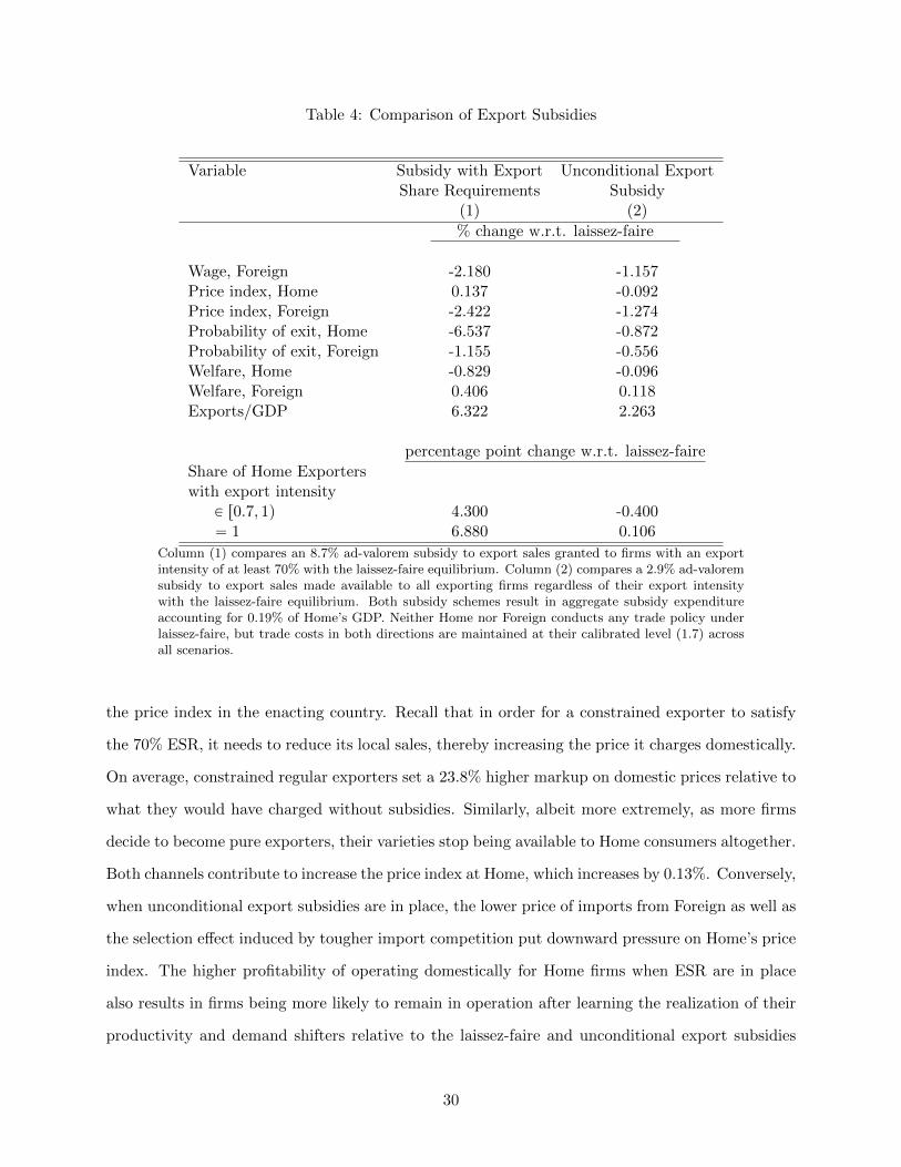
Table 4: Comparison of Export Subsidies

Variable Subsidy with Export Unconditional ExportShare Requirements Subsidy

(1) (2)

% change w.r.t. laissez-faire

Wage, Foreign -2.180 -1.157Price index, Home 0.137 -0.092Price index, Foreign -2.422 -1.274Probability of exit, Home -6.537 -0.872Probability of exit, Foreign -1.155 -0.556Welfare, Home -0.829 -0.096Welfare, Foreign 0.406 0.118Exports/GDP 6.322 2.263

percentage point change w.r.t. laissez-faire

Share of Home Exporterswith export intensity

P r0.7, 1q 4.300 -0.400“ 1 6.880 0.106

Column (1) compares an 8.7% ad-valorem subsidy to export sales granted to firms with an exportintensity of at least 70% with the laissez-faire equilibrium. Column (2) compares a 2.9% ad-valoremsubsidy to export sales made available to all exporting firms regardless of their export intensitywith the laissez-faire equilibrium. Both subsidy schemes result in aggregate subsidy expenditureaccounting for 0.19% of Home’s GDP. Neither Home nor Foreign conducts any trade policy underlaissez-faire, but trade costs in both directions are maintained at their calibrated level (1.7) acrossall scenarios.

the price index in the enacting country. Recall that in order for a constrained exporter to satisfy

the 70% ESR, it needs to reduce its local sales, thereby increasing the price it charges domestically.

On average, constrained regular exporters set a 23.8% higher markup on domestic prices relative to

what they would have charged without subsidies. Similarly, albeit more extremely, as more firms

decide to become pure exporters, their varieties stop being available to Home consumers altogether.

Both channels contribute to increase the price index at Home, which increases by 0.13%. Conversely,

when unconditional export subsidies are in place, the lower price of imports from Foreign as well as

the selection effect induced by tougher import competition put downward pressure on Home’s price

index. The higher profitability of operating domestically for Home firms when ESR are in place

also results in firms being more likely to remain in operation after learning the realization of their

productivity and demand shifters relative to the laissez-faire and unconditional export subsidies

30

scenarios.

We find that the subsidy with ESR has a quantitatively important effect on aggregate outcomes.

The subsidy with ESR boosts exports (as a share of GDP) by 6.32%, while the unconditional sub-

sidy only increases this share by 2.26%. The imposition of an export requirement also reduces

the likelihood of firm exit more than the unconditional subsidy — a 6.5% reduction relative to

laissez-faire instead of the 0.87% fall produced by the latter. Crucially, the additional distortions

introduced by the ESR result in a substantially larger welfare loss for the enacting country; real

income at Home falls by 0.83% with ESR, while the equivalent unconditional export subsidy re-

sults in a 0.096% welfare loss. Foreign, on the other hand, benefits from the availability of cheaper

imported goods from Home, but its perceived welfare gain is always lower than Home’s loss.

Using an Alternative Natural Export Intensity Benchmark. One concern regarding our

calibration strategy is that the undistorted distribution of export intensity is based on countries

that are too different from China in terms of their openness to trade and attractiveness as a location

to set up multinational affiliates.31 Since the corporate income tax deduction conditioned on a 70%

ESR in China was terminated in 2008, and fully phased out by 2013, we explore the robustness of

our results by using the export intensity distribution observed in China in 2013 as the ‘undistorted’

scenario to recalibrate our model parameters using the same target moments as in our benchmark

above.32 It is important to keep in mind, however, that other policy measures featuring export

requirements are likely to remain in place in 2013, and these can bias our estimation of China’s

natural export intensity distribution toward high export intensity levels.

Figure 6 presents the distribution of export intensity for Chinese manufacturing firms sampled

by the WBES in 2002 and 2013. Crucially, the distribution in 2002 is quite similar to the one

calculated with the more representative survey carried out by the Chinese National Bureau of

Statistics (NBS) and presented in Figure 1 — more precisely, the shares of regular exporters with

an export intensity of at least 70% and pure exporters in the 2002 wave of WBES are 23% and 17.3%

respectively; the same shares in the NBS survey are 24.9% and 24.5%. The similitude displayed

31As Antras and Yeaple (2014) note, multinational firms’ affiliates tend to be larger, more productive, and crucially,more export-oriented than non-multinational firms.

32In a Papers & Proceedings article (Defever and Riano, 2015a), we have used the distribution of export intensityobserved in China in 2013 to illustrate the effect of a subsidy with a 100% ESR in a simplified version of our modelwithout firm-destination-specific demand shifters.

31

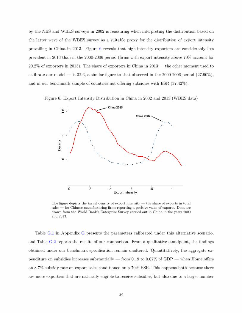
by the NBS and WBES surveys in 2002 is reassuring when interpreting the distribution based on

the latter wave of the WBES survey as a suitable proxy for the distribution of export intensity

prevailing in China in 2013. Figure 6 reveals that high-intensity exporters are considerably less

prevalent in 2013 than in the 2000-2006 period (firms with export intensity above 70% account for

20.2% of exporters in 2013). The share of exporters in China in 2013 — the other moment used to

calibrate our model — is 32.6, a similar figure to that observed in the 2000-2006 period (27.90%),

and in our benchmark sample of countries not offering subsidies with ESR (37.42%).

Figure 6: Export Intensity Distribution in China in 2002 and 2013 (WBES data)

China 2013

China 2002

The figure depicts the kernel density of export intensity — the share of exports in totalsales — for Chinese manufacturing firms reporting a positive value of exports. Data aredrawn from the World Bank’s Enterprise Survey carried out in China in the years 2000and 2013.

Table G.1 in Appendix G presents the parameters calibrated under this alternative scenario,

and Table G.2 reports the results of our comparison. From a qualitative standpoint, the findings

obtained under our benchmark specification remain unaltered. Quantitatively, the aggregate ex-

penditure on subsidies increases substantially — from 0.19 to 0.67% of GDP — when Home offers

an 8.7% subsidy rate on export sales conditioned on a 70% ESR. This happens both because there

are more exporters that are naturally eligible to receive subsidies, but also due to a larger number

32

of firms choosing to become constrained exporters. Under this parametrization the overall effect of

subsidies on the strength of domestic competition, exports and welfare is considerably larger than

in our benchmark.

Further Robustness Analysis. We investigate further the robustness of our results by perturbing

individual model parameters in our benchmark scenario to ensure that our conclusions are not

unduly driven by our chosen parametrization. Thus, we increase one parameter of interest at a

time by 10% relative to its value in the benchmark calibration and report the comparison between

equilibria with subsidies conditioned on ESR and laissez-faire. The results of this exercise are

presented in Table H.1 in Appendix H. Our quantitative results are indeed remarkably robust to

changes in the parametrization of the model.

6 Conclusions

China’s successful insertion into the global economy has spurred great interest in the economic

policies that made this feat possible. In this paper we have documented the widespread use of

subsidies subject to export share requirements in China implemented after the opening-up reforms

in the late 1970s, and yet, still in place after China joined the WTO in 2001 — a practice that

has proven to be a contentious issue with other member countries. We have studied how this

policy affects individual firms’ pricing and production decisions as well as its effects on the level

of competition and aggregate welfare through the lens of a two-country model of trade with firm

heterogeneity across productivity and demand appeal.

Our model shows that offering subsidies with ESR distorts the distribution of export intensity

(conditional on exporting) in a country, skewing it towards the right. Crucially, the imposition

of a single ESR strictly below 100% can induce firms to either increase their domestic prices and

decrease their export prices so as to satisfy the constraint threshold, or, to stop producing for the

domestic market altogether becoming pure exporters. In our quantitative exercise, we evaluate the

impact of one country offering an 8.7% ad-valorem export sales subsidy subject to a 70% ESR —

a policy of similar magnitude to a corporate income tax rate reduction available to foreign-owned

firms and domestically-owned firms located in free trade zones between 1991 and 2008. Our results

33

show that a subsidy with ESR of this magnitude can account for approximately 43% of the share

of exporters in China exhibiting an export intensity of at least 70%, with the majority of these

being pure exporters, a feature which is consistent with the data. We find that subsidies with

ESR increase aggregate exports more and provide greater protection to low-profitability firms than

an equivalent unconditional export subsidy — resulting in protectionism through exporting. The

distortions induced by the subsidy subject to ESR, however exacerbate the welfare losses produced

by the standard textbook export subsidy.

Our findings open up exciting avenues for future research. It would be interesting, for instance,

to understand the political economy objectives that have motivated China and other developing

countries to employ incentives subject to export requirements. These policies could provide a

politically-feasible alternative to full unilateral trade liberalization by eliciting the support of do-

mestic producers, which are likely to be negatively affected by greater trade openness. Another

interesting line of inquiry has to do with the dynamic consequences of subsidies subject to ESR.

Our current analysis has shown that they produce substantial static welfare losses; however it is

possible that if these subsidies help to foster rapid industrialization, their dynamic gains could more

than compensate the distortions that we have identified in this paper.

References

Anderson, J. E. and E. van Wincoop (2004): “Trade Costs,” Journal of Economic Literature,42, 691–751.

Antras, P. and S. R. Yeaple (2014): “Multinational Firms and the Structure of InternationalTrade,” in Handbook of International Economics, ed. by G. Gopinath, E. Helpman, and K. Rogoff,Elsevier, vol. 4, 55 – 130.

Arkolakis, C. (2010): “Market Penetration Costs and the New Consumers Margin in Interna-tional Trade,” Journal of Political Economy, 118, 1151 – 1199.

Bajona, C. and T. Chu (2010): “Reforming State Owned Enterprises in China: Effects of WTOAccession,” Review of Economic Dynamics, 13, 800–823.

Bauer, C., R. B. Davies, and A. Haufler (2014): “Economic Integration and the OptimalCorporate Tax Structure with Heterogeneous Firms,” Journal of Public Economics, 110, 42–56.

Bernard, A. B., J. Eaton, J. B. Jensen, and S. Kortum (2003): “Plants and Productivityin International Trade,” American Economic Review, 93, 1268–1290.

Bernard, A. B., J. B. Jensen, S. J. Redding, and P. K. Schott (2007): “Firms in Inter-national Trade,” Journal of Economic Perspectives, 21, 105–130.

34

Brandt, L. and P. M. Morrow (2013): “Tariffs and the Organization of Trade in China,”Manuscript, University of Toronto.

Brandt, L., J. van Biesebroeck, and Y. Zhang (2012): “Creative Accounting or Creative De-struction? Firm-level Productivity Growth in Chinese Manufacturing ?” Journal of DevelopmentEconomics, 97, 339–351.

——— (2014): “Challenges of Working with the Chinese NBS Firm-Level Data,” China EconomicReview, 30, 339–352.

Branstetter, L. G. and R. C. Feenstra (2002): “Trade and Foreign Direct Investment inChina: a Political Economy Approach,” Journal of International Economics, 58, 335–358.

Branstetter, L. G. and N. R. Lardy (2008): “China’s Embrace of Globalization,” in China’sGreat Economic Transformation, ed. by L. Brandt and T. G. Rawski, Cambridge: CambridgeUniversity Press.

Broda, C., J. Greenfield, and D. Weinstein (2006): “From Groundnuts to Globalization: AStructural Estimate of Trade and Growth,” NBER Working Papers 12512, National Bureau ofEconomic Research.

Broda, C. and D. E. Weinstein (2006): “Globalization and the Gains from Variety,” TheQuarterly Journal of Economics, 121, 541–585.

Chan, T., E. K. Y. Chen, and S. Chin (1986): “China’s Special Economic Zones: Ideology,Policy and Practice,” in China’s Special Economic Zones: Policies, Problems and Prospects, ed.by Y. C. Jao and C. K. Leung, Oxford: Oxford University Press.

Chao, C.-C. and E. S. H. Yu (2014): Trade-Related Investment Measures: Theory and Appli-cations, London: Imperial College Press.

Cherkashin, I., S. Demidova, H. L. Kee, and K. Krishna (2015): “Firm Heterogeneity andCostly Trade: A New Estimation Strategy and Policy Experiments,” Journal of InternationalEconomics, 96, 18–36.

Chor, D. (2009): “Subsidies for FDI: Implications From a Model with Heterogeneous Firms,”Journal of International Economics, 78, 113–125.

Claro, S. (2006): “Supporting Inefficient Firms with Capital Subsidies: China and Germany inthe 1990s,” Journal of Comparative Economics, 34, 377–401.

Costinot, A., A. Rodrıguez-Clare, and I. Werning (2015): “Micro to Macro: OptimalTrade Policy with Firm Heterogeneity,” Manuscript, MIT.

Creskoff, S. and P. Walkenhorst (2009): “Implications of WTO Disciplines for SpecialEconomic Zones in Developing Countries,” World Bank Policy Research Working Paper 4892.

Crozet, M., K. Head, and T. Mayer (2012): “Quality Sorting and Trade: Firm-level Evidencefor French Wine,” Review of Economic Studies, 79, 609–644.

Dai, M., M. Maitra, and M. Yu (2011): “Unexceptional Exporter Performance in China? TheRole of Processing Trade,” Manuscript, Columbia University.

35

Davidson, C., S. J. Matusz, and M. E. Kreinin (1985): “Analysis of Performance Standardsfor Direct Foreign Investments,” Canadian Journal of Economics, 18, 876–90.

Davies, R. B. and C. Eckel (2010): “Tax Competition for Heterogeneous Firms with Endoge-nous Entry,” American Economic Journal: Economic Policy, 2, 77–102.

Defever, F. and A. Riano (2015a): “Gone for Good? Subsidies with Export Share Requirementsin China: 2002-2013,” World Bank Economic Review Papers & Proceedings, 29, S125–S144.

——— (2015b): “Twin Peaks,” Manuscript, University of Nottingham.

Demidova, S. and A. Rodrıguez-Clare (2009): “Trade Policy Under Firm-level Heterogeneityin a Small Economy,” Journal of International Economics, 78, 100–112.

Dıaz de Astarloa, B., J. Eaton, K. Krishna, B. Y. Aw-Roberts, A. Rodrıguez-Clare,and J. Tybout (2013): “Born-to-Export Firms: Understanding Export Growth in Bangladesh,”International Growth Centre Working Paper.

Eaton, J., S. Kortum, and F. Kramarz (2011): “An Anatomy of International Trade: EvidenceFrom French Firms,” Econometrica, 79, 1453–1498.

Feenstra, R. C. (1998): “One Country, Two Systems: Implications of WTO Entry for China,”Manuscript, University of California, Davis.

Feenstra, R. C. and S.-J. Wei (2010): “Introduction to “China’s Growing Role in WorldTrade”,” in China’s Growing Role in World Trade, National Bureau of Economic Research,1–31.

Felbermayr, G., B. Jung, and M. Larch (2012): “Optimal Tariffs, Retaliation and the WelfareLoss from Tariff Wars in the Melitz Model,” Journal of International Economics, 89, 13–25.

Fernandes, A. P. and H. Tang (2012): “Determinants of Vertical Integration in Export Pro-cessing: Theory and Evidence from China,” Journal of Development Economics, 99, 396–414.

Girma, S., Y. Gong, H. Gorg, and Z. Yu (2009): “Can Production Subsidies Explain China’sExport Performance? Evidence from Firm-level Data,” Scandinavian Journal of Economics, 111,863–891.

Haley, U. C. V. and G. T. Haley (2013): Subsidies to Chinese Industry: State Capitalism,Business Strategy and Trade Policy, Oxford: Oxford University Press.

Hamada, K. (1974): “An Economic Analysis of the Duty Free Zone,” Journal of InternationalEconomics, 4, 225–241.

Hanson, G. H. (2012): “The Rise of Middle Kingdoms: Emerging Economies in Global Trade,”Journal of Economic Perspectives, 26, 41–64.

Helpman, E., M. J. Melitz, and S. R. Yeaple (2004): “Export Versus FDI with HeterogeneousFirms,” American Economic Review, 94, 300–316.

Holmes, T. J., E. R. McGrattan, and E. C. Prescott (Forthcoming): “Quid Pro Quo:Technology Capital Transfers for Market Access in China,” Review of Economic Studies.

36

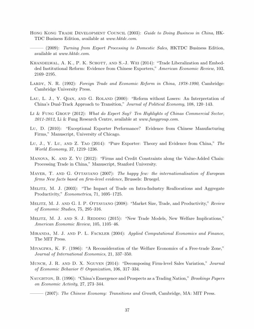
Hong Kong Trade Development Council (2003): Guide to Doing Business in China, HK-TDC Business Edition, available at www.hktdc.com.

——— (2009): Turning from Export Processing to Domestic Sales, HKTDC Business Edition,available at www.hktdc.com.

Khandelwal, A. K., P. K. Schott, and S.-J. Wei (2014): “Trade Liberalization and Embed-ded Institutional Reform: Evidence from Chinese Exporters,” American Economic Review, 103,2169–2195.

Lardy, N. R. (1992): Foreign Trade and Economic Reform in China, 1978-1990, Cambridge:Cambridge University Press.

Lau, L. J., Y. Qian, and G. Roland (2000): “Reform without Losers: An Interpretation ofChina’s Dual-Track Approach to Transition,” Journal of Political Economy, 108, 120–143.

Li & Fung Group (2012): What do Expert Say? Ten Highlights of Chinas Commercial Sector,2011-2012, Li & Fung Research Centre, available at www.funggroup.com.

Lu, D. (2010): “Exceptional Exporter Performance? Evidence from Chinese ManufacturingFirms,” Manuscript, University of Chicago.

Lu, J., Y. Lu, and Z. Tao (2014): “Pure Exporter: Theory and Evidence from China,” TheWorld Economy, 37, 1219–1236.

Manova, K. and Z. Yu (2012): “Firms and Credit Constraints along the Value-Added Chain:Processing Trade in China,” Manuscript, Stanford University.

Mayer, T. and G. Ottaviano (2007): The happy few: the internationalisation of Europeanfirms New facts based on firm-level evidence, Brussels: Bruegel.

Melitz, M. J. (2003): “The Impact of Trade on Intra-Industry Reallocations and AggregateProductivity,” Econometrica, 71, 1695–1725.

Melitz, M. J. and G. I. P. Ottaviano (2008): “Market Size, Trade, and Productivity,” Reviewof Economic Studies, 75, 295–316.

Melitz, M. J. and S. J. Redding (2015): “New Trade Models, New Welfare Implications,”American Economic Review, 105, 1105–46.

Miranda, M. J. and P. L. Fackler (2004): Applied Computational Economics and Finance,The MIT Press.

Miyagiwa, K. F. (1986): “A Reconsideration of the Welfare Economics of a Free-trade Zone,”Journal of International Economics, 21, 337–350.

Munch, J. R. and D. X. Nguyen (2014): “Decomposing Firm-level Sales Variation,” Journalof Economic Behavior & Organization, 106, 317–334.

Naughton, B. (1996): “China’s Emergence and Prospects as a Trading Nation,” Brookings Paperson Economic Activity, 27, 273–344.

——— (2007): The Chinese Economy: Transitions and Growth, Cambridge, MA: MIT Press.

37

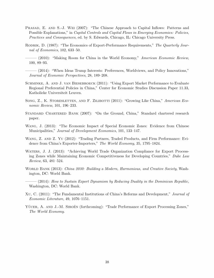
Prasad, E. and S.-J. Wei (2007): “The Chinese Approach to Capital Inflows: Patterns andPossible Explanations,” in Capital Controls and Capital Flows in Emerging Economies: Policies,Practices and Consequences, ed. by S. Edwards, Chicago, IL: Chicago University Press.

Rodrik, D. (1987): “The Economics of Export-Performance Requirements,” The Quarterly Jour-nal of Economics, 102, 633–50.

——— (2010): “Making Room for China in the World Economy,” American Economic Review,100, 89–93.

——— (2014): “When Ideas Trump Interests: Preferences, Worldviews, and Policy Innovations,”Journal of Economic Perspectives, 28, 189–208.

Schminke, A. and J. van Biesebroeck (2011): “Using Export Market Performance to EvaluateRegional Preferential Policies in China,” Center for Economic Studies Discussion Paper 11.33,Katholieke Universiteit Leuven.

Song, Z., K. Storesletten, and F. Zilibotti (2011): “Growing Like China,” American Eco-nomic Review, 101, 196–233.

Standard Chartered Bank (2007): “On the Ground, China,” Standard chartered researchpaper.

Wang, J. (2013): “The Economic Impact of Special Economic Zones: Evidence from ChineseMunicipalities,” Journal of Development Economics, 101, 133–147.

Wang, Z. and Z. Yu (2012): “Trading Partners, Traded Products, and Firm Performance: Evi-dence from China’s Exporter-Importers,” The World Economy, 35, 1795–1824.

Waters, J. J. (2013): “Achieving World Trade Organization Compliance for Export Process-ing Zones while Maintaining Economic Competitiveness for Developing Countries,” Duke LawReview, 63, 481–524.

World Bank (2013): China 2030: Building a Modern, Harmonious, and Creative Society, Wash-ington, DC: World Bank.

——— (2014): How to Sustain Export Dynamism by Reducing Duality in the Dominican Republic,Washington, DC: World Bank.

Xu, C. (2011): “The Fundamental Institutions of China’s Reforms and Development,” Journal ofEconomic Literature, 49, 1076–1151.

Yucer, A. and J.-M. Siroen (forthcoming): “Trade Performance of Export Processing Zones,”The World Economy.

38

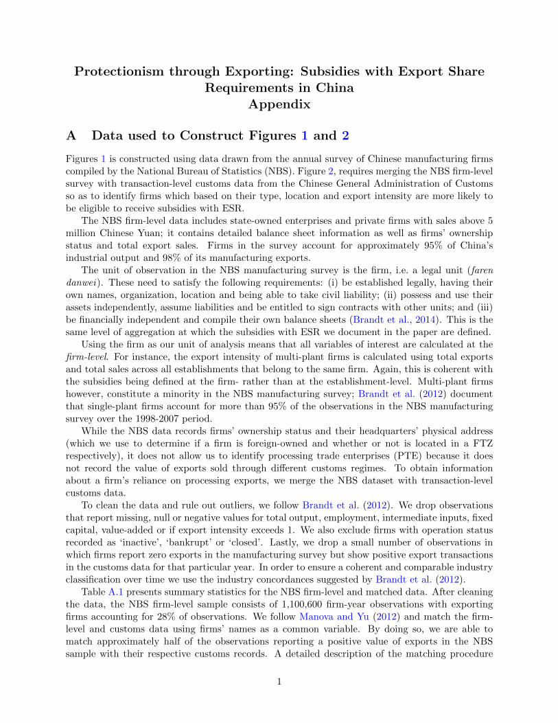
Protectionism through Exporting: Subsidies with Export ShareRequirements in China

Appendix

A Data used to Construct Figures 1 and 2

Figures 1 is constructed using data drawn from the annual survey of Chinese manufacturing firmscompiled by the National Bureau of Statistics (NBS). Figure 2, requires merging the NBS firm-levelsurvey with transaction-level customs data from the Chinese General Administration of Customsso as to identify firms which based on their type, location and export intensity are more likely tobe eligible to receive subsidies with ESR.

The NBS firm-level data includes state-owned enterprises and private firms with sales above 5million Chinese Yuan; it contains detailed balance sheet information as well as firms’ ownershipstatus and total export sales. Firms in the survey account for approximately 95% of China’sindustrial output and 98% of its manufacturing exports.

The unit of observation in the NBS manufacturing survey is the firm, i.e. a legal unit (farendanwei). These need to satisfy the following requirements: (i) be established legally, having theirown names, organization, location and being able to take civil liability; (ii) possess and use theirassets independently, assume liabilities and be entitled to sign contracts with other units; and (iii)be financially independent and compile their own balance sheets (Brandt et al., 2014). This is thesame level of aggregation at which the subsidies with ESR we document in the paper are defined.

Using the firm as our unit of analysis means that all variables of interest are calculated at thefirm-level. For instance, the export intensity of multi-plant firms is calculated using total exportsand total sales across all establishments that belong to the same firm. Again, this is coherent withthe subsidies being defined at the firm- rather than at the establishment-level. Multi-plant firmshowever, constitute a minority in the NBS manufacturing survey; Brandt et al. (2012) documentthat single-plant firms account for more than 95% of the observations in the NBS manufacturingsurvey over the 1998-2007 period.

While the NBS data records firms’ ownership status and their headquarters’ physical address(which we use to determine if a firm is foreign-owned and whether or not is located in a FTZrespectively), it does not allow us to identify processing trade enterprises (PTE) because it doesnot record the value of exports sold through different customs regimes. To obtain informationabout a firm’s reliance on processing exports, we merge the NBS dataset with transaction-levelcustoms data.

To clean the data and rule out outliers, we follow Brandt et al. (2012). We drop observationsthat report missing, null or negative values for total output, employment, intermediate inputs, fixedcapital, value-added or if export intensity exceeds 1. We also exclude firms with operation statusrecorded as ‘inactive’, ‘bankrupt’ or ‘closed’. Lastly, we drop a small number of observations inwhich firms report zero exports in the manufacturing survey but show positive export transactionsin the customs data for that particular year. In order to ensure a coherent and comparable industryclassification over time we use the industry concordances suggested by Brandt et al. (2012).

Table A.1 presents summary statistics for the NBS firm-level and matched data. After cleaningthe data, the NBS firm-level sample consists of 1,100,600 firm-year observations with exportingfirms accounting for 28% of observations. We follow Manova and Yu (2012) and match the firm-level and customs data using firms’ names as a common variable. By doing so, we are able tomatch approximately half of the observations reporting a positive value of exports in the NBSsample with their respective customs records. A detailed description of the matching procedure

1

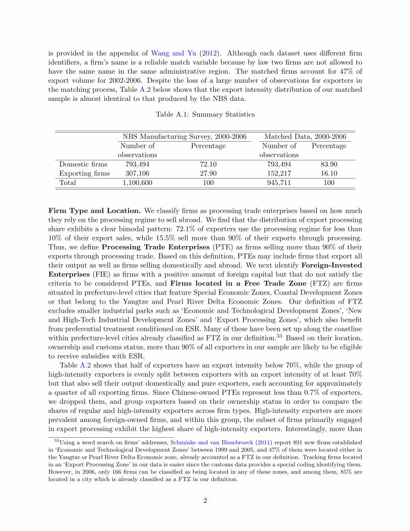
is provided in the appendix of Wang and Yu (2012). Although each dataset uses different firmidentifiers, a firm’s name is a reliable match variable because by law two firms are not allowed tohave the same name in the same administrative region. The matched firms account for 47% ofexport volume for 2002-2006. Despite the loss of a large number of observations for exporters inthe matching process, Table A.2 below shows that the export intensity distribution of our matchedsample is almost identical to that produced by the NBS data.

Table A.1: Summary Statistics

NBS Manufacturing Survey, 2000-2006 Matched Data, 2000-2006

Number of Percentage Number of Percentageobservations observations

Domestic firms 793,494 72.10 793,494 83.90Exporting firms 307,106 27.90 152,217 16.10

Total 1,100,600 100 945,711 100

Firm Type and Location. We classify firms as processing trade enterprises based on how muchthey rely on the processing regime to sell abroad. We find that the distribution of export processingshare exhibits a clear bimodal pattern: 72.1% of exporters use the processing regime for less than10% of their export sales, while 15.5% sell more than 90% of their exports through processing.Thus, we define Processing Trade Enterprises (PTE) as firms selling more than 90% of theirexports through processing trade. Based on this definition, PTEs may include firms that export alltheir output as well as firms selling domestically and abroad. We next identify Foreign-InvestedEnterprises (FIE) as firms with a positive amount of foreign capital but that do not satisfy thecriteria to be considered PTEs, and Firms located in a Free Trade Zone (FTZ) are firmssituated in prefecture-level cities that feature Special Economic Zones, Coastal Development Zonesor that belong to the Yangtze and Pearl River Delta Economic Zones. Our definition of FTZexcludes smaller industrial parks such as ‘Economic and Technological Development Zones’, ‘Newand High-Tech Industrial Development Zones’ and ‘Export Processing Zones’, which also benefitfrom preferential treatment conditioned on ESR. Many of these have been set up along the coastlinewithin prefecture-level cities already classified as FTZ in our definition.33 Based on their location,ownership and customs status, more than 90% of all exporters in our sample are likely to be eligibleto receive subsidies with ESR.

Table A.2 shows that half of exporters have an export intensity below 70%, while the group ofhigh-intensity exporters is evenly split between exporters with an export intensity of at least 70%but that also sell their output domestically and pure exporters, each accounting for approximatelya quarter of all exporting firms. Since Chinese-owned PTEs represent less than 0.7% of exporters,we dropped them, and group exporters based on their ownership status in order to compare theshares of regular and high-intensity exporters across firm types. High-intensity exporters are moreprevalent among foreign-owned firms, and within this group, the subset of firms primarily engagedin export processing exhibit the highest share of high-intensity exporters. Interestingly, more than

33Using a word search on firms’ addresses, Schminke and van Biesebroeck (2011) report 891 new firms establishedin ‘Economic and Technological Development Zones’ between 1999 and 2005, and 47% of them were located either inthe Yangtze or Pearl River Delta Economic zone, already accounted as a FTZ in our definition. Tracking firms locatedin an ‘Export Processing Zone’ in our data is easier since the customs data provides a special coding identifying them.However, in 2006, only 166 firms can be classified as being located in any of these zones, and among them, 85% arelocated in a city which is already classified as a FTZ in our definition.

2

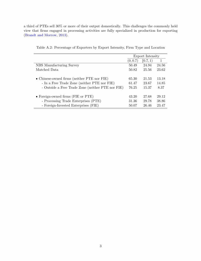
a third of PTEs sell 30% or more of their output domestically. This challenges the commonly heldview that firms engaged in processing activities are fully specialized in production for exporting(Brandt and Morrow, 2013).

Table A.2: Percentage of Exporters by Export Intensity, Firm Type and Location

Export Intensity

p0, 0.7q r0.7, 1q 1

NBS Manufacturing Survey 50.49 24.94 24.56Matched Data 50.82 25.56 23.62

‚ Chinese-owned firms (neither PTE nor FIE) 65.30 21.53 13.18- In a Free Trade Zone (neither PTE nor FIE) 61.47 23.67 14.85- Outside a Free Trade Zone (neither PTE nor FIE) 76.25 15.37 8.37

‚ Foreign-owned firms (FIE or PTE) 43.20 27.68 29.12- Processing Trade Enterprises (PTE) 31.36 29.78 38.86- Foreign-Invested Enterprises (FIE) 50.07 26.46 23.47

3

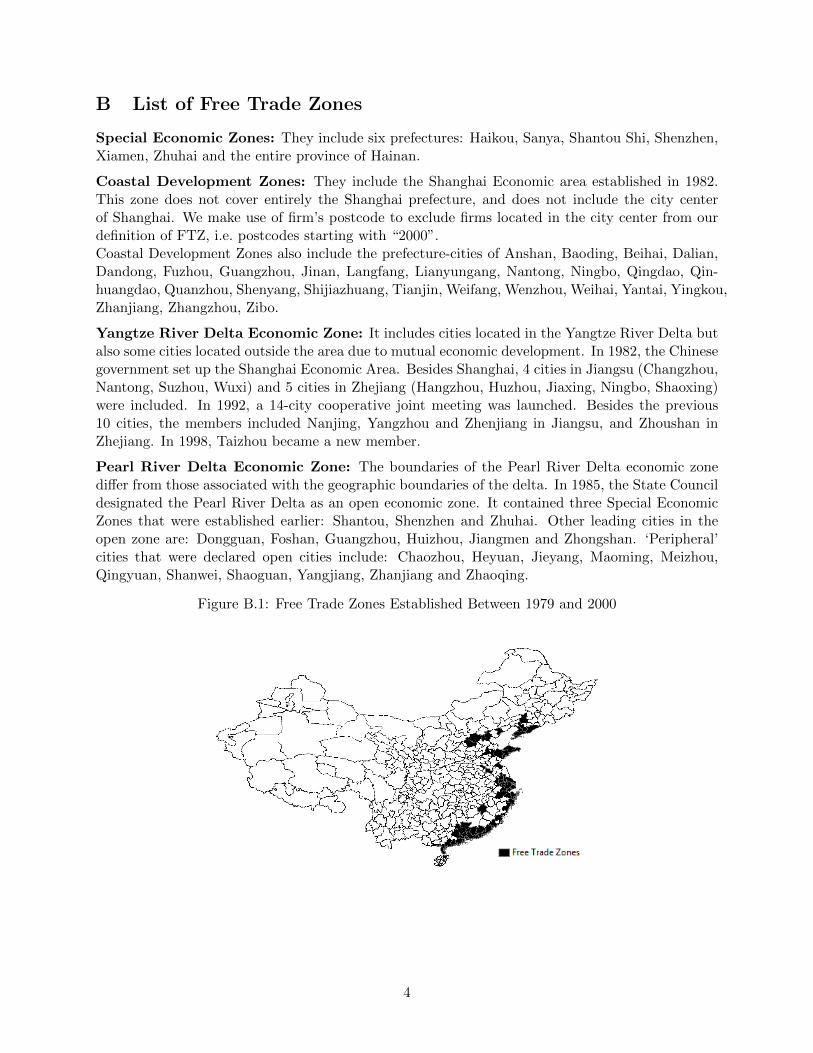
B List of Free Trade Zones

Special Economic Zones: They include six prefectures: Haikou, Sanya, Shantou Shi, Shenzhen,Xiamen, Zhuhai and the entire province of Hainan.

Coastal Development Zones: They include the Shanghai Economic area established in 1982.This zone does not cover entirely the Shanghai prefecture, and does not include the city centerof Shanghai. We make use of firm’s postcode to exclude firms located in the city center from ourdefinition of FTZ, i.e. postcodes starting with “2000”.Coastal Development Zones also include the prefecture-cities of Anshan, Baoding, Beihai, Dalian,Dandong, Fuzhou, Guangzhou, Jinan, Langfang, Lianyungang, Nantong, Ningbo, Qingdao, Qin-huangdao, Quanzhou, Shenyang, Shijiazhuang, Tianjin, Weifang, Wenzhou, Weihai, Yantai, Yingkou,Zhanjiang, Zhangzhou, Zibo.

Yangtze River Delta Economic Zone: It includes cities located in the Yangtze River Delta butalso some cities located outside the area due to mutual economic development. In 1982, the Chinesegovernment set up the Shanghai Economic Area. Besides Shanghai, 4 cities in Jiangsu (Changzhou,Nantong, Suzhou, Wuxi) and 5 cities in Zhejiang (Hangzhou, Huzhou, Jiaxing, Ningbo, Shaoxing)were included. In 1992, a 14-city cooperative joint meeting was launched. Besides the previous10 cities, the members included Nanjing, Yangzhou and Zhenjiang in Jiangsu, and Zhoushan inZhejiang. In 1998, Taizhou became a new member.

Pearl River Delta Economic Zone: The boundaries of the Pearl River Delta economic zonediffer from those associated with the geographic boundaries of the delta. In 1985, the State Councildesignated the Pearl River Delta as an open economic zone. It contained three Special EconomicZones that were established earlier: Shantou, Shenzhen and Zhuhai. Other leading cities in theopen zone are: Dongguan, Foshan, Guangzhou, Huizhou, Jiangmen and Zhongshan. ‘Peripheral’cities that were declared open cities include: Chaozhou, Heyuan, Jieyang, Maoming, Meizhou,Qingyuan, Shanwei, Shaoguan, Yangjiang, Zhanjiang and Zhaoqing.

Figure B.1: Free Trade Zones Established Between 1979 and 2000

4

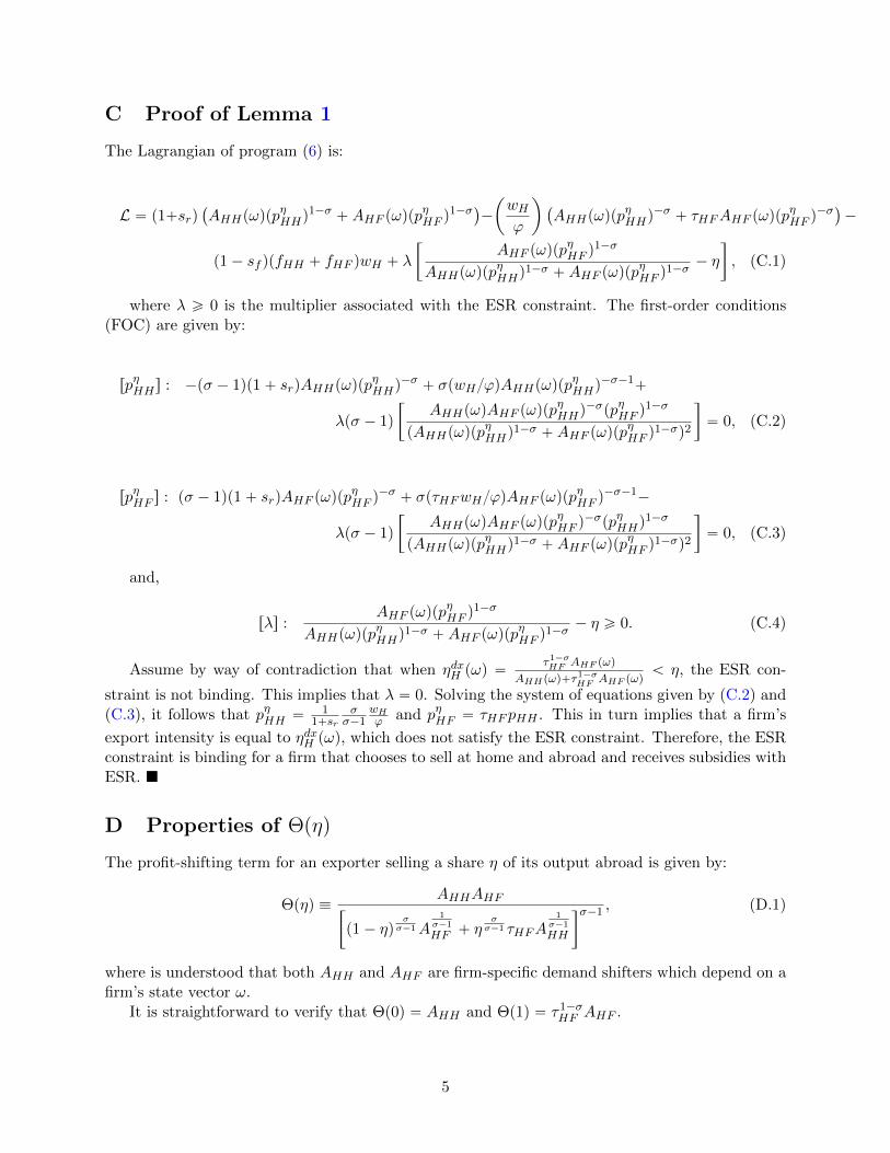
C Proof of Lemma 1

The Lagrangian of program (6) is:

L “ p1`srq`

AHHpωqppηHHq

1´σ `AHF pωqppηHF q

1´σ˘

´

ˆ

wHϕ

˙

`

AHHpωqppηHHq

´σ ` τHFAHF pωqppηHF q

´σ˘

´

p1´ sf qpfHH ` fHF qwH ` λ

„

AHF pωqppηHF q

1´σ

AHHpωqppηHHq

1´σ `AHF pωqppηHF q

1´σ´ η

, (C.1)

where λ ě 0 is the multiplier associated with the ESR constraint. The first-order conditions(FOC) are given by:

rpηHHs : ´pσ ´ 1qp1` srqAHHpωqppηHHq

´σ ` σpwHϕqAHHpωqppηHHq

´σ´1`

λpσ ´ 1q

„

AHHpωqAHF pωqppηHHq

´σppηHF q1´σ

pAHHpωqppηHHq

1´σ `AHF pωqppηHF q

1´σq2

“ 0, (C.2)

rpηHF s : pσ ´ 1qp1` srqAHF pωqppηHF q

´σ ` σpτHFwHϕqAHF pωqppηHF q

´σ´1´

λpσ ´ 1q

„

AHHpωqAHF pωqppηHF q

´σppηHHq1´σ

pAHHpωqppηHHq

1´σ `AHF pωqppηHF q

1´σq2

“ 0, (C.3)

and,

rλs :AHF pωqpp

ηHF q

1´σ

AHHpωqppηHHq

1´σ `AHF pωqppηHF q

1´σ´ η ě 0. (C.4)

Assume by way of contradiction that when ηdxH pωq “τ1´σHF AHF pωq

AHHpωq`τ1´σHF AHF pωq

ă η, the ESR con-

straint is not binding. This implies that λ “ 0. Solving the system of equations given by (C.2) and(C.3), it follows that pηHH “

11`sr

σσ´1

wHϕ and pηHF “ τHF pHH . This in turn implies that a firm’s

export intensity is equal to ηdxH pωq, which does not satisfy the ESR constraint. Therefore, the ESRconstraint is binding for a firm that chooses to sell at home and abroad and receives subsidies withESR.

D Properties of Θpηq

The profit-shifting term for an exporter selling a share η of its output abroad is given by:

Θpηq ”AHHAHF

„

p1´ ηqσσ´1A

1σ´1

HF ` ησσ´1 τHFA

1σ´1

HH

σ´1 , (D.1)

where is understood that both AHH and AHF are firm-specific demand shifters which depend on afirm’s state vector ω.

It is straightforward to verify that Θp0q “ AHH and Θp1q “ τ1´σHF AHF .

5

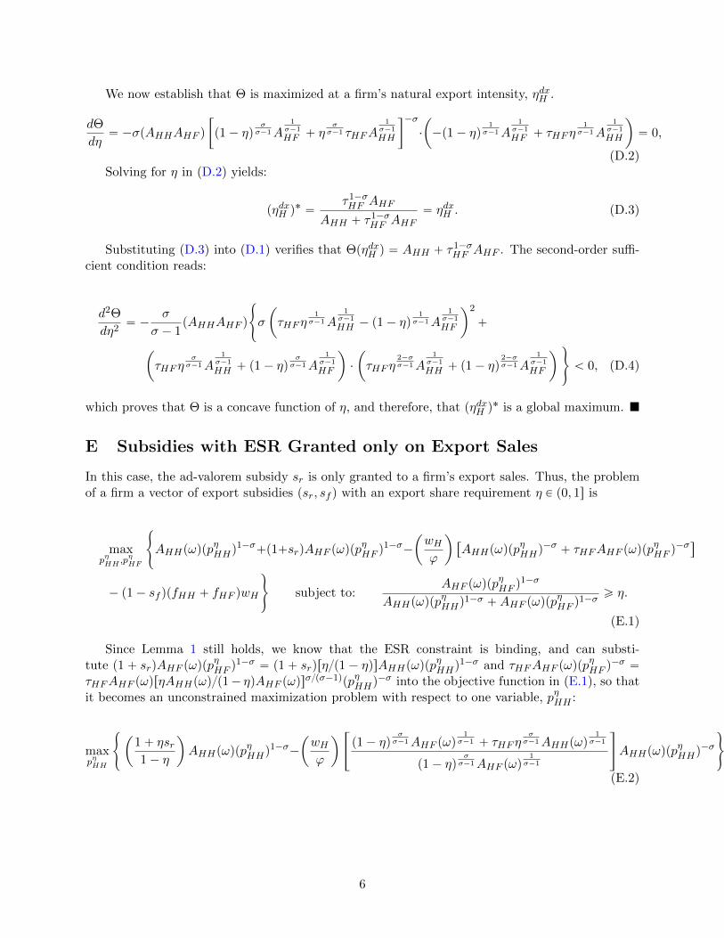
We now establish that Θ is maximized at a firm’s natural export intensity, ηdxH .

dΘ

dη“ ´σpAHHAHF q

„

p1´ ηqσσ´1A

1σ´1

HF ` ησσ´1 τHFA

1σ´1

HH

´σ

¨

ˆ

´p1´ ηq1

σ´1A1

σ´1

HF ` τHF η1

σ´1A1

σ´1

HH

˙

“ 0,

(D.2)Solving for η in (D.2) yields:

pηdxH q˚ “

τ1´σHF AHF

AHH ` τ1´σHF AHF

“ ηdxH . (D.3)

Substituting (D.3) into (D.1) verifies that ΘpηdxH q “ AHH ` τ1´σHF AHF . The second-order suffi-

cient condition reads:

d2Θ

dη2“ ´

σ

σ ´ 1pAHHAHF q

#

σ

ˆ

τHF η1

σ´1A1

σ´1

HH ´ p1´ ηq1

σ´1A1

σ´1

HF

˙2

`

ˆ

τHF ησσ´1A

1σ´1

HH ` p1´ ηqσσ´1A

1σ´1

HF

˙

¨

ˆ

τHF η2´σσ´1A

1σ´1

HH ` p1´ ηq2´σσ´1A

1σ´1

HF

˙

+

ă 0, (D.4)

which proves that Θ is a concave function of η, and therefore, that pηdxH q˚ is a global maximum.

E Subsidies with ESR Granted only on Export Sales

In this case, the ad-valorem subsidy sr is only granted to a firm’s export sales. Thus, the problemof a firm a vector of export subsidies psr, sf q with an export share requirement η P p0, 1s is

maxpηHH ,p

ηHF

#

AHHpωqppηHHq

1´σ`p1`srqAHF pωqppηHF q

1´σ´

ˆ

wHϕ

˙

“

AHHpωqppηHHq

´σ ` τHFAHF pωqppηHF q

´σ‰

´ p1´ sf qpfHH ` fHF qwH

+

subject to:AHF pωqpp

ηHF q

1´σ

AHHpωqppηHHq

1´σ `AHF pωqppηHF q

1´σě η.

(E.1)

Since Lemma 1 still holds, we know that the ESR constraint is binding, and can substi-tute p1` srqAHF pωqpp

ηHF q

1´σ “ p1` srqrηp1´ ηqsAHHpωqppηHHq

1´σ and τHFAHF pωqppηHF q

´σ “

τHFAHF pωqrηAHHpωqp1´ ηqAHF pωqsσpσ´1qppηHHq

´σ into the objective function in (E.1), so thatit becomes an unconstrained maximization problem with respect to one variable, pηHH :

maxpηHH

#

ˆ

1` ηsr1´ η

˙

AHHpωqppηHHq

1´σ´

ˆ

wHϕ

˙

«

p1´ ηqσσ´1AHF pωq

1σ´1 ` τHF η

σσ´1AHHpωq

1σ´1

p1´ ηqσσ´1AHF pωq

1σ´1

ff

AHHpωqppηHHq

´σ

+

.

(E.2)

6

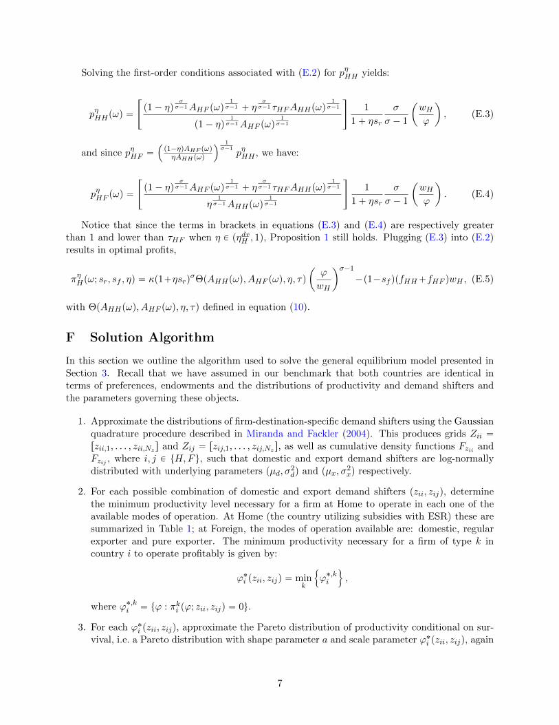
Solving the first-order conditions associated with (E.2) for pηHH yields:

pηHHpωq “

«

p1´ ηqσσ´1AHF pωq

1σ´1 ` η

σσ´1 τHFAHHpωq

1σ´1

p1´ ηq1

σ´1AHF pωq1

σ´1

ff

1

1` ηsr

σ

σ ´ 1

ˆ

wHϕ

˙

, (E.3)

and since pηHF “´

p1´ηqAHF pωqηAHHpωq

¯1

σ´1pηHH , we have:

pηHF pωq “

«

p1´ ηqσσ´1AHF pωq

1σ´1 ` η

σσ´1 τHFAHHpωq

1σ´1

η1

σ´1AHHpωq1

σ´1

ff

1

1` ηsr

σ

σ ´ 1

ˆ

wHϕ

˙

. (E.4)

Notice that since the terms in brackets in equations (E.3) and (E.4) are respectively greaterthan 1 and lower than τHF when η P pηdxH , 1q, Proposition 1 still holds. Plugging (E.3) into (E.2)results in optimal profits,

πηHpω; sr, sf , ηq “ κp1`ηsrqσΘpAHHpωq, AHF pωq, η, τq

ˆ

ϕ

wH

˙σ´1

´p1´sf qpfHH`fHF qwH , (E.5)

with ΘpAHHpωq, AHF pωq, η, τq defined in equation (10).

F Solution Algorithm

In this section we outline the algorithm used to solve the general equilibrium model presented inSection 3. Recall that we have assumed in our benchmark that both countries are identical interms of preferences, endowments and the distributions of productivity and demand shifters andthe parameters governing these objects.

1. Approximate the distributions of firm-destination-specific demand shifters using the Gaussianquadrature procedure described in Miranda and Fackler (2004). This produces grids Zii “rzii,1, . . . , zii,Nz s and Zij “ rzij,1, . . . , zij,Nz s, as well as cumulative density functions Fzii andFzij , where i, j P tH,F u, such that domestic and export demand shifters are log-normallydistributed with underlying parameters pµd, σ

2dq and pµx, σ

2xq respectively.

2. For each possible combination of domestic and export demand shifters pzii, zijq, determinethe minimum productivity level necessary for a firm at Home to operate in each one of theavailable modes of operation. At Home (the country utilizing subsidies with ESR) these aresummarized in Table 1; at Foreign, the modes of operation available are: domestic, regularexporter and pure exporter. The minimum productivity necessary for a firm of type k incountry i to operate profitably is given by:

ϕ˚i pzii, zijq “ mink

!

ϕ˚,ki

)

,

where ϕ˚,ki “ tϕ : πki pϕ; zii, zijq “ 0u.

3. For each ϕ˚i pzii, zijq, approximate the Pareto distribution of productivity conditional on sur-vival, i.e. a Pareto distribution with shape parameter a and scale parameter ϕ˚i pzii, zijq, again

7

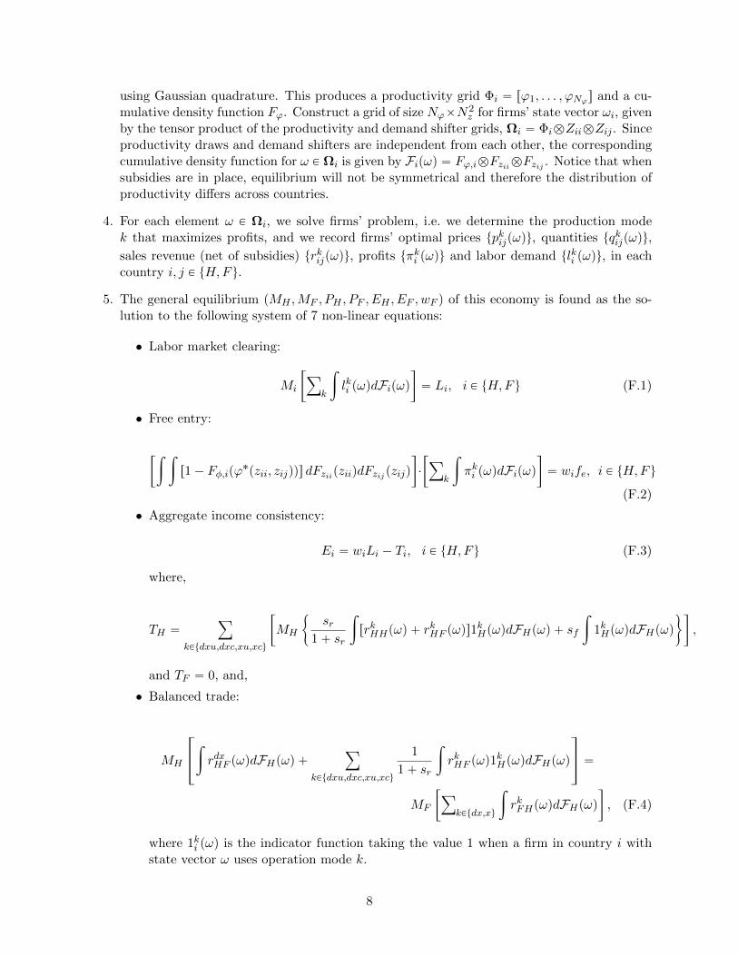
using Gaussian quadrature. This produces a productivity grid Φi “ rϕ1, . . . , ϕNϕs and a cu-mulative density function Fϕ. Construct a grid of size NϕˆN

2z for firms’ state vector ωi, given

by the tensor product of the productivity and demand shifter grids, Ωi “ ΦibZiibZij . Sinceproductivity draws and demand shifters are independent from each other, the correspondingcumulative density function for ω P Ωi is given by Fipωq “ Fϕ,ibFziibFzij . Notice that whensubsidies are in place, equilibrium will not be symmetrical and therefore the distribution ofproductivity differs across countries.

4. For each element ω P Ωi, we solve firms’ problem, i.e. we determine the production modek that maximizes profits, and we record firms’ optimal prices tpkijpωqu, quantities tqkijpωqu,

sales revenue (net of subsidies) trkijpωqu, profits tπki pωqu and labor demand tlki pωqu, in eachcountry i, j P tH,F u.

5. The general equilibrium pMH ,MF , PH , PF , EH , EF , wF q of this economy is found as the so-lution to the following system of 7 non-linear equations:

• Labor market clearing:

Mi

„

ÿ

k

ż

lki pωqdFipωq

“ Li, i P tH,F u (F.1)

• Free entry:

„ż ż

r1´ Fφ,ipϕ˚pzii, zijqqs dFziipziiqdFzij pzijq

¨

„

ÿ

k

ż

πki pωqdFipωq

“ wife, i P tH,F u

(F.2)

• Aggregate income consistency:

Ei “ wiLi ´ Ti, i P tH,F u (F.3)

where,

TH “ÿ

kPtdxu,dxc,xu,xcu

„

MH

"

sr1` sr

ż

rrkHHpωq ` rkHF pωqs1

kHpωqdFHpωq ` sf

ż

1kHpωqdFHpωq*

,

and TF “ 0, and,

• Balanced trade:

MH

»

–

ż

rdxHF pωqdFHpωq `ÿ

kPtdxu,dxc,xu,xcu

1

1` sr

ż

rkHF pωq1kHpωqdFHpωq

fi

fl “

MF

„

ÿ

kPtdx,xu

ż

rkFHpωqdFHpωq

, (F.4)

where 1ki pωq is the indicator function taking the value 1 when a firm in country i withstate vector ω uses operation mode k.

8

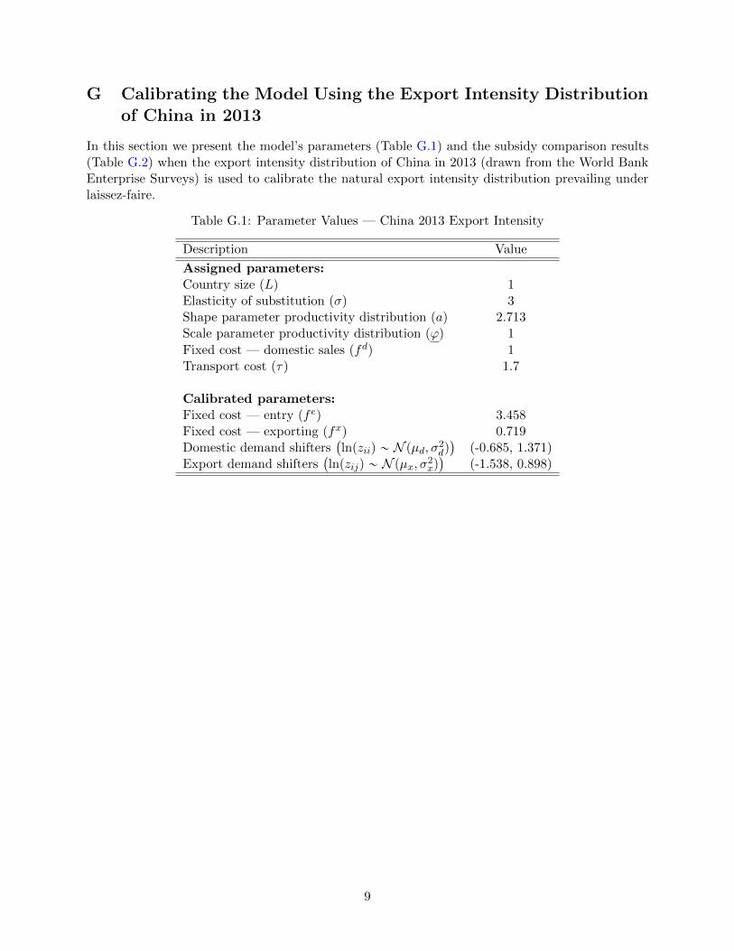
G Calibrating the Model Using the Export Intensity Distributionof China in 2013

In this section we present the model’s parameters (Table G.1) and the subsidy comparison results(Table G.2) when the export intensity distribution of China in 2013 (drawn from the World BankEnterprise Surveys) is used to calibrate the natural export intensity distribution prevailing underlaissez-faire.

Table G.1: Parameter Values — China 2013 Export Intensity

Description Value

Assigned parameters:Country size (L) 1Elasticity of substitution (σ) 3Shape parameter productivity distribution (a) 2.713Scale parameter productivity distribution (ϕ) 1

Fixed cost — domestic sales (fd) 1Transport cost (τ) 1.7

Calibrated parameters:Fixed cost — entry (fe) 3.458Fixed cost — exporting (fx) 0.719Domestic demand shifters

`

lnpziiq „ N pµd, σ2dq˘

(-0.685, 1.371)Export demand shifters

`

lnpzijq „ N pµx, σ2xq˘

(-1.538, 0.898)

9

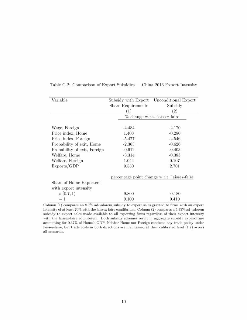
Table G.2: Comparison of Export Subsidies — China 2013 Export Intensity

Variable Subsidy with Export Unconditional ExportShare Requirements Subsidy

(1) (2)

% change w.r.t. laissez-faire

Wage, Foreign -4.484 -2.170Price index, Home 1.403 -0.280Price index, Foreign -5.477 -2.546Probability of exit, Home -2.363 -0.626Probability of exit, Foreign -0.912 -0.403Welfare, Home -3.314 -0.383Welfare, Foreign 1.044 0.107Exports/GDP 9.550 2.701

percentage point change w.r.t. laissez-faire

Share of Home Exporterswith export intensity

P r0.7, 1q 9.800 -0.180“ 1 9.100 0.410

Column (1) compares an 8.7% ad-valorem subsidy to export sales granted to firms with an exportintensity of at least 70% with the laissez-faire equilibrium. Column (2) compares a 5.35% ad-valoremsubsidy to export sales made available to all exporting firms regardless of their export intensitywith the laissez-faire equilibrium. Both subsidy schemes result in aggregate subsidy expenditureaccounting for 0.67% of Home’s GDP. Neither Home nor Foreign conducts any trade policy underlaissez-faire, but trade costs in both directions are maintained at their calibrated level (1.7) acrossall scenarios.

10

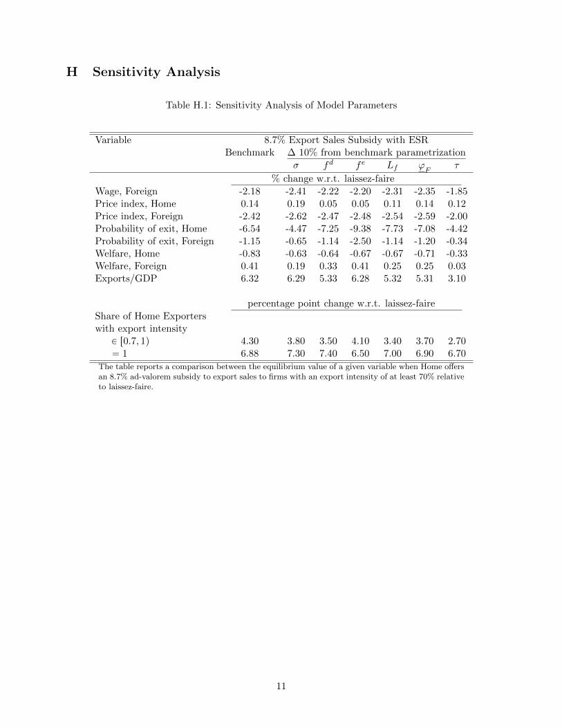
H Sensitivity Analysis

Table H.1: Sensitivity Analysis of Model Parameters

Variable 8.7% Export Sales Subsidy with ESRBenchmark ∆ 10% from benchmark parametrization

σ fd fe Lf ϕF

τ

% change w.r.t. laissez-faire

Wage, Foreign -2.18 -2.41 -2.22 -2.20 -2.31 -2.35 -1.85Price index, Home 0.14 0.19 0.05 0.05 0.11 0.14 0.12Price index, Foreign -2.42 -2.62 -2.47 -2.48 -2.54 -2.59 -2.00Probability of exit, Home -6.54 -4.47 -7.25 -9.38 -7.73 -7.08 -4.42Probability of exit, Foreign -1.15 -0.65 -1.14 -2.50 -1.14 -1.20 -0.34Welfare, Home -0.83 -0.63 -0.64 -0.67 -0.67 -0.71 -0.33Welfare, Foreign 0.41 0.19 0.33 0.41 0.25 0.25 0.03Exports/GDP 6.32 6.29 5.33 6.28 5.32 5.31 3.10

percentage point change w.r.t. laissez-faire

Share of Home Exporterswith export intensity

P r0.7, 1q 4.30 3.80 3.50 4.10 3.40 3.70 2.70“ 1 6.88 7.30 7.40 6.50 7.00 6.90 6.70

The table reports a comparison between the equilibrium value of a given variable when Home offersan 8.7% ad-valorem subsidy to export sales to firms with an export intensity of at least 70% relativeto laissez-faire.

11

CENTRE FOR ECONOMIC PERFORMANCE Recent Discussion Papers

1430 Andrew B. Bernard Renzo Massari Jose-Daniel Reyes Daria Taglioni

Exporter Dynamics and Partial-Year Effects

1429 Cletus C. Coughlin Dennis Novy

Estimating Border Effects: The Impact of Spatial Aggregation

1428 Alan Manning The Elusive Employment Effect of the Minimum Wage

1427 Decio Coviello Andrea Guglielmo Giancarlo Spagnolo

The Effect of Discretion on Procurement Performance

1426 Andrew B. Bernard Andreas Moxnes and Karen Helene Ulltveit-Moe

Two-sided Heterogeneity and Trade

1425 Stephen Machin Sandra McNally Martina Viarengo

“Teaching to Teach” Literacy

1424 Yatang Lin Where does the Wind Blow? Green Preferences and Spatial Misallocation in the Renewable Energy Sector

1423 Andrew B. Bernard Valerie Smeets Frederic Warzynski

Rethinking Deindustrialization

1422 Stefano Gagliarducci Marco Manacorda

Politics in the Family: Nepotism and the Hiring Decisions of Italian Firms

1421 Jordi Blanes i Vidal Marc Möller

Team Adaptation

1420 Andrew B. Bernard J. Bradford Jensen Stephen J. Redding Peter K. Schott

Global Firms

1419 Marco Manacorda Andrea Tesei

Liberation Technology: Mobile Phones and Political Mobilization in Africa

1418 Jeremiah Dittmar Ralf R. Meisenzahl

State Capacity and Public Goods: Institutional Change, Human Capital and Growth in Early Modern Germany

1417 Holger Breinlich Swati Dhingra Gianmarco Ottaviano

How Have EU’s Trade Agreements Impacted Consumers?

1416 Stefan Bender Nicholas Bloom David Card John Van Reenen Stefanie Wolter

Management Practices, Workforce Selection and Productivity

1415 Emanuel Ornelas Special and Differential Treatment for Developing Countries

1414 Markus K. Brunnermeier Luis Garicano Philip R. Lane Marco Pagano Ricardo Reis Tano Santos David Thesmar Stijn Van Nieuwerburgh Dimitri Vayanos

The Sovereign-Bank Diabolic Loop and ESBies

1413 Antoine Dechezleprêtre Elias Einiö Ralf Martin Kieu-Trang Nguyen John Van Reenen

Do Tax Incentives for Research Increase Firm Innovation? An RD Design for R&D

The Centre for Economic Performance Publications Unit Tel 020 7955 7673 Fax 020 7404 0612

Email info@cep.lse.ac.uk Web site http://cep.lse.ac.uk