ISSN 2042-2695

CEP Discussion Paper No 1082

September 2011

A Many-Country Model of Industrialization

Holger Breinlich and Alejandro Cuñat

Abstract We draw attention to the role of economic geography in explaining important cross-sectional

facts which are difficult to account for in existing models of industrialization. By

construction, closed-economy models that stress the role of local demand in generating

sufficient expenditure on manufacturing goods are not suited to explain the strong and

negative correlation between distance to the world’s main markets and levels of

manufacturing activity in the developing world. Secondly, open-economy models that

emphasize the importance of comparative advantage are at odds with a positive correlation

between the ratio of agricultural to manufacturing productivity and shares of manufacturing

in GDP. This paper provides a potential explanation for these puzzles by nesting the above

theories in a multi-location model with trade costs. Using a number of simple analytical

examples and a full-scale multi-country calibration, we show that the model can replicate the

above stylized facts.

Keywords: Industrialization, economic geography, international trade

JEL Classifications: F11, F12, F14, O14

This paper was produced as part of the Centre’s Globalisation Programme. The Centre for

Economic Performance is financed by the Economic and Social Research Council.

Acknowledgements This paper is partly based on the unpublished 2005 paper ‘Economic Geography and

Industrialization’ which was Chapter 2 of Breinlich’s PhD dissertation. We are grateful to

Harald Fadinger, Gabriel Felbermayr and seminar participants in Mannheim, Munich and

Vienna for helpful suggestions. Stephen Redding, Anthony Venables and Silvana Tenreyro

provided very useful comments on the earlier PhD chapter. All remaining errors are ours.

Holger Breinlich is a Research Associate of the Centre for Economic Performance,

London School of Economics and Lecturer in the Department of Economics, University of

Essex. Alejandro Cuñat is a Professor of Economics, University of Vienna.

Published by

Centre for Economic Performance

London School of Economics and Political Science

Houghton Street

London WC2A 2AE

All rights reserved. No part of this publication may be reproduced, stored in a retrieval

system or transmitted in any form or by any means without the prior permission in writing of

the publisher nor be issued to the public or circulated in any form other than that in which it

is published.

Requests for permission to reproduce any article or part of the Working Paper should be sent

to the editor at the above address.

H. Breinlich and A. Cuñat, submitted 2011

1 Introduction

One of the most striking aspects of economic development is the decline of agriculture’s share

in GDP and the corresponding rise of manufacturing and services. Economists have proposed a

number of theories to explain this transformation. Among the most influential approaches are

explanations that focus on differences in the income elasticity of demand across sectors (e.g.,

Rosenstein-Rodan (1943); Murphy et al. (1989b); Kongsamut et al. (2001)). As per-capita

income increases, non-homothetic preferences lead to a shift of demand from agriculture to man-

ufacturing goods, thus increasing manufacturing’s share in GDP. Traditionally, these approaches

have analyzed closed-economy models and stressed the role of local demand. More recently, au-

thors such as Matsuyama (1992, 2009) have provided extensions to open-economy settings and

have shown that some key results of the closed-economy literature, such as the positive impact

of increased agricultural productivity on industrialization, can be reversed in such models.

The present paper draws attention to two cross-sectional facts which, taken together, are not

easily explained by either closed-economy or open-economy models of demand-driven industrial-

ization. We argue that to understand these facts we need to move beyond the closed-versus-open-

economy dichotomy prevalent in the literature, and to consider multi-country settings in which

countries interact with each other through international trade, but in which bilateral interactions

are partly hampered (to a different extent across country pairs) by the fact that trade is not

costless.

Our first observation is that proximity to foreign sources of demand seems to matter for

industrialization. For example, it has long been noted that Hong Kong, Singapore, and Taiwan

not only benefitted from an outward-oriented trade policy but also close proximity to the large

Japanese market (e.g., Puga and Venables (1996)). A cursory look at the data suggests that

distance to foreign markets has a more general relevance: Figure 1 plots the manufacturing share

in GDP against the minimum distance to the European Union, Japan and the U.S. for a cross-

section of developing countries in 2000.1 The figure shows that developing economies close to one

of these main markets of the world show proportionally higher levels of industrialization.

Whereas this first fact suggests that interactions between economies are important, and thus

points to the relevance of open-economy models, our second fact seems to suggest the oppo-

site: Figure 2 plots manufacturing shares against a standard proxy for comparative advantage

in agriculture, labor productivity in agriculture relative to manufacturing, for a cross-section of

developing countries for the year 2000.2 The fitted line has a positive, albeit statistically insignif-

icant slope. As we show in our more detailed econometric analysis in Section 2, extending the

sample to include more countries and years leaves this positive correlation intact and actually

makes it statistically significant as well. This is of course puzzling for open-economy theories of

1We use the Netherlands as the approximate geographic centre of the European Union in Figure 1. Developingcountries are defined as countries belonging to the income categories “low”, “lower middle” and “upper middle”published by the World Bank (corresponding to less than 9,265 USD in 1999). The simple OLS regression underlyingthe fitted line in Figure 1 yields a negative slope coeffi cient which is statistically significant at the 1% level.

2Developing countries are defined as in footnote 1. Relative productivy in agriculture vs. manufacturing is theproxy of choice in many studies of Ricardian comparative advantage, e.g. Golub and Hsieh (2000).

2

industrialization such as Matsuyama (1992). If countries are indeed integrated through trade,

should we not expect them to specialize according to their comparative advantages?

We argue that both facts can be understood in a standard model of industrialization in which

there are differences in the income elasticity of demand across sectors and in which comparative

advantage forces are present and active. The key difference of our approach in comparison with

existing closed-economy approaches is that we allow for a setting with many countries which

are integrated through trade. But crucially, and in contrast to open-economy models such as

Matsuyama (1992), trade is not costless and geographic position is therefore important.

In our model, developing countries closer to foreign sources of demand will experience higher

demand for both the agricultural and manufacturing goods they produce than more distant coun-

tries, ceteris paribus. We outline conditions under which this translates into higher manufacturing

shares in GDP. Most importantly, higher overall demand will lead to higher wages which, in the

presence of non-homotheticity in demand combined with positive trade costs, will shift local

production towards the manufacturing sector. Trade costs for agricultural products also ham-

per the comparative-advantage mechanism put forward by free-trade models. High agricultural

productivity leads to higher wages which, again because of the combination of agricultural trade

costs and non-homothetic demand, leads countries to specialize in manufacturing (we call this

the “relative-demand effect”of agricultural productivity). The standard comparative-advantage

effect, which would drive specialization patterns in the opposite direction, is also present but can

be overcompensated by the relative-demand effect for intermediate levels of trade costs.

Given that our model nests free trade and autarky as special cases and that its predictions

vary depending on the level of trade costs and other parameters (such as the degree of non-

homotheticity of preferences), we complement our theoretical analysis with a full-scale multi-

country calibration. That is, we ask to what extent our model matches the above stylized facts

for empirically plausible parameter values. We choose parameters to match international trade

and expenditure data and demonstrate that this calibrated model generates the same positive

correlation observed in the data between access to markets and comparative advantage in agri-

culture, on the one hand, and manufacturing shares on the other hand. Crucially, this is not true

when we constrain our trade cost estimates to zero (free trade) or infinity (autarky). Interest-

ingly, allowing for positive but finite levels of trade costs also improves the predictive power (in

terms of matching observed and predicted shares) as opposed to autarky and free trade.

Our paper relates to at least three sets of contributions in the literature. In terms of the

questions addressed, we contribute most directly to the literature on industrialization that relies

on differences in the income elasticity of demand across sectors for explaining structural change

(“demand-driven industrialization”). We add to this literature by drawing attention to the role

of economic geography in shaping cross-sectional patterns of industrialization. Similar to papers

such as Murphy et al. (1989a, b), Matsuyama (1992) or Laitner (2000) we focus on the initial

shift from agriculture to manufacturing, which is the key transition for the group of countries we

are interested in in this paper, i.e. low- to middle-income countries. That is, for most of the paper

we do not model the services sector, which rises with income per capita at all levels of economic

3

development, and which is not subject to open-economy analytical treatments due to its non-

tradability. However, as we show in our robustness checks, explicitly modelling a non-tradable

services sector leaves our results unchanged.

Consistent with our focus on explaining cross-sectional facts, we also disregard the dynamic

aspects of the industrialization process and rely on an entirely static model. In this respect, we

are similar to the contributions by Murphy et al. (1989a, b) and Matsuyama (2009) but different

from most other papers in the industrialization literature. Our approach, however, avoids the

criticism by Ventura (1997) and Matsuyama (2009), among others, of closed-economy dynamic

approaches to issues such as industrialization; namely that explaining cross-country patterns

taking place in a globalized world on the basis of dynamic closed-economy arguments can be

quite misleading. In fact, we extend this methodological criticism to the standard two-country,

free-trade way of thinking about trade and development: once one recognizes that bilateral

distances and geographic position matter, one must extend the model to many countries and

allow for differences in bilateral trade costs.

While our criticisms apply most directly to theories that approach the phenomenon of in-

dustrialization from the demand side, the stylized facts we have presented are not easily ex-

plained by models that focus on supply-side determinants either, be it contributions from the

barriers-to-modern-growth literature (e.g., Parente and Prescott (1994) and (2000), Goodfriend

and McDermott (1995), or Galor and Weil (2000)), attempts to reconcile balanced (neoclassical)

growth or convergence with structural transformations (e.g., Caselli and Coleman (2001) or Ngai

and Pissarides (2007)) or approaches from traditional international trade theory (e.g., Leamer

(1987) and Schott (2003)). The ageographical nature of these approaches means that they are not

well suited to explain phenomena that have an inherent geographic component, such as the ones

described above. Thus, while not denying the importance of these models and theories for many

aspects of industrialization, this paper draws attention to geographical proximity as a new and

potentially important factor in explaining the dramatic differences in levels of industrialization

across the world.3

Methodologically, our paper is most closely related to work in international trade and eco-

nomic geography which is interested in the effects of comparative advantage and relative location

on trade flows, wages, and production structures (e.g., Krugman (1980), Puga and Venables

(1999), Golub and Hsieh (2000), Davis and Weinstein (2003), or Redding and Venables (2004),

to name but a few). To the best of our knowledge, however, the insights from this literature have

never been applied to the aforementioned stylized facts, nor to the modelling of cross-sectional

patterns in levels of industrialization more generally. Some of our results are also relevant for the

international trade literature beyond our immediate focus on industrialization. For example, the

role of trade costs in modifying the impact of comparative advantage on production structures

3 In a recent working paper, Yi and Zhang (2010) share our concern that many aspects of industrializationcannot be analyzed neither within a closed-economy setting nor under free trade. They analyze the effects ofchanges in productivity and declining trade barriers on production structures within a three-sector, two-countrymodel, but focus on dynamic rather than cross-sectional aspects of industrialization. Restricting their analysis toa two-country setting also prevents them from adequately modelling economic geography. (For this, at least threecountries are needed as will become clear in Section 3).

4

has been mostly ignored in the literature, although our results suggest that models based on a

free-trade assumption may have poor explanatory power.4 Theoretically, we contribute to the

home-market effect literature by outlining conditions under which more central locations special-

ize in manufacturing once we leave the standard setting of monopolistic competition and factor

price equalization.5

The remainder of this paper is organized as follows. Section 2 shows that the two correlations

displayed in Figures 1 and 2 also survive in a broader cross-section of countries, and are robust to

the inclusion of proxies for local demand and other domestic factors. Section 3 develops a multi-

country model with trade costs. This model is used in Section 4 to shed light on the puzzles

raised in the introduction. In Section 5 we show that a fully calibrated version of the model is

able to replicate our stylized facts. Finally, section 6 concludes.

2 Empirical Evidence

In this section, we examine the robustness of the correlations from the introduction through

variations in sample composition and by including a number of control variables.6 Our full

econometric specification will be

ltShareMlt = α+ dt + β1RPlt + β2CENlt + β3APlt + β4POPlt + εlt, (1)

where RPlt is relative productivity (of agriculture to manufacturing) and CENlt the ‘centrality’

of country l, i.e., its access to foreign markets (to be defined below). APlt denotes agricultural

productivity, POPlt the population size of country l, and dt is a full set of year fixed effects.

The dependent variable is the logistic transformation of a country’s share of manufacturing value

added in GDP. We use a logistic transformation to account for the fact the manufacturing share is

limited to a range between 0 and 1.7 Concerning the regressors, we discuss the choice of suitable

empirical proxies in turn. Additional details on the data and their sources, as well as a list of

countries used in the regressions below are contained in Appendix A.

Keeping in line with existing studies on Ricardian comparative advantage (e.g., Golub and

Hsieh, 2000), we use labor productivity as a proxy for productivity. In contrast to total factor

productivity, this has the advantage of considerably increasing the number of available observa-

tions.

We measure country l’s centrality (CENlt) as the sum of all other countries’GNP, weighted

4An exception is Deardorff (2004).5Also see Davis (1998) and Hanson and Xiang (2004).6These are the correlations we will aim at reproducing in our calibration exercise.7Using untransformed manufacturing shares instead does not change any of the qualitative results reported

below. We have also experimented with including the share of services in GDP as an additional control variable,again without finding any significant changes in the other coeffi cient estimates (both sets of results are availablefrom the authors upon request).

5

by the inverse of bilateral distances, which are taken to proxy for trade costs between locations:

CENl =∑j 6=l

GNPj × dist−1jl . (2)

This specification reflects the basic intuition of our discussion. What matters is centrality in an

economic geography sense, that is proximity to markets for domestic products. Of course, the

above centrality index is closely related to the concept of market potential first proposed by Harris

(1954), which has been frequently used in both geography and —more recently —in economics. A

number of studies have demonstrated that this simple proxy has strong explanatory power and

yields results very similar to more complex approaches that estimate trade costs from trade flow

gravity equations (see, for example, Head and Mayer (2006), or Breinlich (2006)).8

As additional control variables, we also include agricultural productiviy (AP ) to account for

the pro-industrializing relative-demand effect discussed above, and population size (POP ) as an

additional proxy for the extent of the domestic market. We have data for all the required variables

for 112 countries in 2000. Keeping in line with the focus of this paper on the industrialization

of developing countries, however, we exclude high-income countries from our regression sample

(although of course all available countries are used to calculate the centrality measure).9 In our

robustness checks, we will also briefly present results for the full sample.10

In Table 1, we present a number of univariate correlations between the logistic transformation

of manufacturing shares and our proxies for comparative advantage (relative productivity, RP )

and centrality. Columns 1-2 replicate the correlations from Figures 1 and 2 and show that using a

logistic transformation of manufacturing shares as the dependent variable leads to similar results.

In column 3, we use our more sophisticated measure of centrality (2). Note that we would now

expect to find a positive and significant sign, which is indeed what we do. We also note that both

measures of centrality seem to be important determinants of levels of industrialization. They

explain around 10% of the cross-sectional variation of manufacturing shares in our sample. This

is comparable in magnitude to per-capita income whose positive correlation with manufacturing

shares in the initial phase of development is a key variable in much of the existing empirical

literature on cross-country patterns of industrialization (e.g., Syrquin and Chenery (1989)).

In columns 4-8, we undertake a first series of robustness checks. Column 4 uses data on

sector-specific purchasing power parities to strip out the variation in prices from our relative

productivity measure, so that the remaining variation more closely reflects physical productivity

differences (Appendix C provides additional details). As seen, using this refined measure leaves

the correlation with manufacturing shares basically unchanged. In columns 5-6, we include a

dummy for China and the South-East Asian economies of Korea, Thailand, Malaysia, Indonesia

and the Philippines. These countries are arguably special cases because of their very successful

8Using a nonstructural measure also seems to be better in line with the more explorative character of thissection.

9We use the World Bank’s income classification and exclude all countries with gross national income per capitain excess of 9,265 USD in 1999 (“high income countries”).10See footnote 34 in Section 5 and Appendix Table A.2.

6

export-oriented industrialization strategies and are also potentially influential outliers in both

Figures 1 and 2. The corresponding dummy variable (not reported) is indeed positive and highly

significant but the coeffi cient on our centrality measure remains almost unchanged. The positive

correlation between manufacturing shares and relative productivity is increased and becomes

statistically significant. In columns 7 and 8, we present results for additional years for which

comparable cross-sectional data on relative productivities is available (1980 and 2000, yielding

a unbalanced panel of 256 observations in total). Again, using these additional data makes the

results from columns 1 and 3 stronger.

In Table 2, we gradually build up our results to the full specification (1). In column 1

we include population size, column 2 uses agricultural productivity as an additional regressor,

and column 3 includes both population and agricultural productivity. In column 4, we drop

agricultural productivity and replace it with per-capita GDP. Per-capita GDP helps controlling

for the purchasing power of the local population, skill levels, and other potentially confounding

factors. Note, however, that it is very highly correlated with agricultural productivity so that

in practice both variables are likely to pick up the influence of similar omitted variables. The

high correlation also makes the inclusion of both variables in the same regression impossible.11

In columns 5-8, we again use our larger sample for the years 1980, 1990 and 2000.

Three main insights arise from these regressions. First, proxies for the size of the domestic

market are strongly positively correlated with levels of industrialization, as was to be expected

from prior results in the literature. Second, centrality retains its positive and significant influence

throughout. Third, comparative advantage in agriculture has a positive and significant effect

on industrialization whenever we do not control for absolute agricultural productivity, and an

insignificant effect whenever we do. This suggests that relative productivity might be picking up

the influence of absolute productivity levels in agriculture.

Limited data availability for relative and absolute agricultural productivity prevents us from

estimating specification (1) for a yet larger sample. In columns 9-11, we exclude these variables

which increases the sample size more than tenfold since we can now use observations for every

year from 1980 to 2005. This allows us to provide some further results on the importance of

centrality for industrialization by running variations of the following specification:

ltShareMlt = α+ dt + dl + δ1CENlt + δ2PCGDPlt + δ3POPlt + εlt, (3)

where PCGDPlt denotes per-capita GDP and dt and dl are a full set of time and country fixed

effects. Column 9 of Table 2 reports results for an OLS regression pooled over the period 1980-2005

with year dummies only. Column 10 estimates the full specification (3) by including country fixed

effects, thus eliminating any time-invariant heterogeneity across countries from our correlations.

Column 11 uses long first differences between 1980 and 2005. All regressions give a similar

picture as the results for the smaller sample: both the size of the domestic market and access to

foreign markets are positively correlated with levels of industrialization. If anything, controlling

11The correlations of the variables in logs is 84% in our sample.

7

for country-specific effects in columns 10 and 11 implies an even stronger role for centrality.12

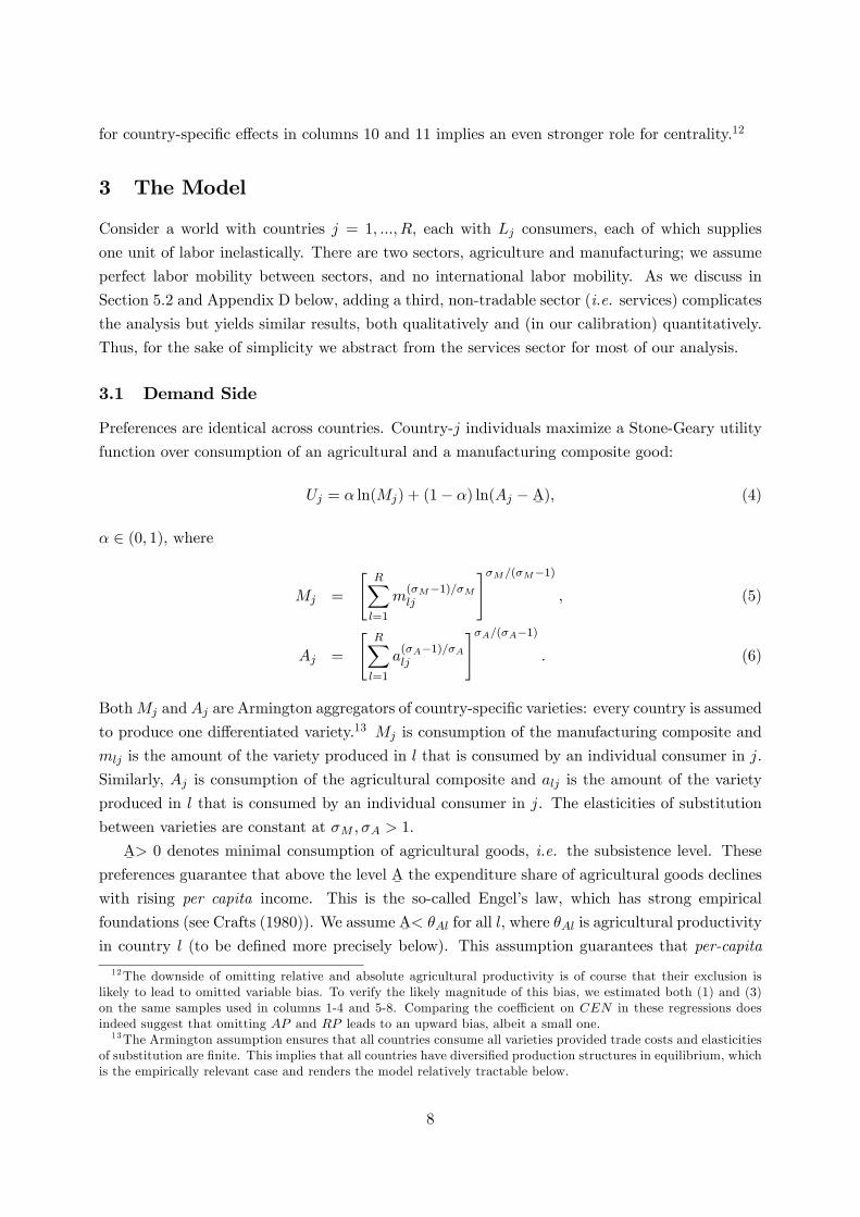
3 The Model

Consider a world with countries j = 1, ..., R, each with Lj consumers, each of which supplies

one unit of labor inelastically. There are two sectors, agriculture and manufacturing; we assume

perfect labor mobility between sectors, and no international labor mobility. As we discuss in

Section 5.2 and Appendix D below, adding a third, non-tradable sector (i.e. services) complicates

the analysis but yields similar results, both qualitatively and (in our calibration) quantitatively.

Thus, for the sake of simplicity we abstract from the services sector for most of our analysis.

3.1 Demand Side

Preferences are identical across countries. Country-j individuals maximize a Stone-Geary utility

function over consumption of an agricultural and a manufacturing composite good:

Uj = α ln(Mj) + (1− α) ln(Aj −A¯ ), (4)

α ∈ (0, 1), where

Mj =

[R∑l=1

m(σM−1)/σMlj

]σM/(σM−1), (5)

Aj =

[R∑l=1

a(σA−1)/σAlj

]σA/(σA−1). (6)

BothMj and Aj are Armington aggregators of country-specific varieties: every country is assumed

to produce one differentiated variety.13 Mj is consumption of the manufacturing composite and

mlj is the amount of the variety produced in l that is consumed by an individual consumer in j.

Similarly, Aj is consumption of the agricultural composite and alj is the amount of the variety

produced in l that is consumed by an individual consumer in j. The elasticities of substitution

between varieties are constant at σM , σA > 1.

A¯> 0 denotes minimal consumption of agricultural goods, i.e. the subsistence level. These

preferences guarantee that above the level A¯the expenditure share of agricultural goods declines

with rising per capita income. This is the so-called Engel’s law, which has strong empirical

foundations (see Crafts (1980)). We assume A¯< θAl for all l, where θAl is agricultural productivity

in country l (to be defined more precisely below). This assumption guarantees that per-capita

12The downside of omitting relative and absolute agricultural productivity is of course that their exclusion islikely to lead to omitted variable bias. To verify the likely magnitude of this bias, we estimated both (1) and (3)on the same samples used in columns 1-4 and 5-8. Comparing the coeffi cient on CEN in these regressions doesindeed suggest that omitting AP and RP leads to an upward bias, albeit a small one.13The Armington assumption ensures that all countries consume all varieties provided trade costs and elasticities

of substitution are finite. This implies that all countries have diversified production structures in equilibrium, whichis the empirically relevant case and renders the model relatively tractable below.

8

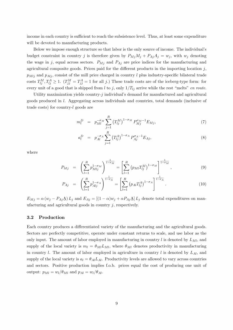
income in each country is suffi cient to reach the subsistence level. Thus, at least some expenditure

will be devoted to manufacturing products.

Below we impose enough structure so that labor is the only source of income. The individual’s

budget constraint in country j is therefore given by PMjMj + PAjAj = wj , with wj denoting

the wage in j, equal across sectors. PMj and PAj are price indices for the manufacturing and

agricultural composite goods. Prices paid for the different products in the importing location j,

pMlj and pAlj , consist of the mill price charged in country l plus industry-specific bilateral trade

costs TMlj , TAlj ≥ 1. (TMjj = TAjj = 1 for all j.) These trade costs are of the iceberg-type form: for

every unit of a good that is shipped from l to j, only 1/Tlj arrive while the rest “melts”en route.

Utility maximization yields country-j individual’s demand for manufactured and agricultural

goods produced in l. Aggregating across individuals and countries, total demands (inclusive of

trade costs) for country-l goods are

mDl = p−σMMl

R∑j=1

(TMlj

)1−σMP σM−1Mj EMj , (7)

aDl = p−σAAl

R∑j=1

(TAlj)1−σA

P σA−1Aj EAj , (8)

where

PMj =

(R∑l=1

p1−σMMlj

) 11−σM

=

[R∑l=1

(pMlT

Mlj

)1−σM] 11−σM

, (9)

PAj =

(R∑l=1

p1−σAAlj

) 11−σA

=

[R∑l=1

(pAlT

Alj

)1−σA] 11−σA

. (10)

EMj = α (wj − PAjA¯ )Lj and EAj = [(1− α)wj + αPAjA¯]Lj denote total expenditures on man-

ufacturing and agricultural goods in country j, respectively.

3.2 Production

Each country produces a differentiated variety of the manufacturing and the agricultural goods.

Sectors are perfectly competitive, operate under constant returns to scale, and use labor as the

only input. The amount of labor employed in manufacturing in country l is denoted by LMl, and

supply of the local variety is ml = θMlLMl, where θMl denotes productivity in manufacturing

in country l. The amount of labor employed in agriculture in country l is denoted by LAl, and

supply of the local variety is al = θAlLAl. Productivity levels are allowed to vary across countries

and sectors. Positive production implies f.o.b. prices equal the cost of producing one unit of

output: pMl = wl/θMl and pAl = wl/θAl.

9

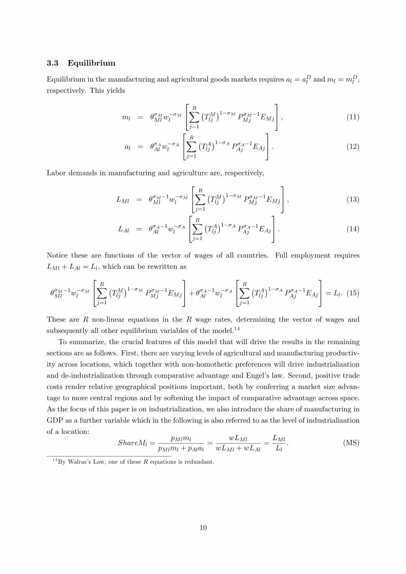
3.3 Equilibrium

Equilibrium in the manufacturing and agricultural goods markets requires al = aDl andml = mDl ,

respectively. This yields

ml = θσMMlw−σMl

R∑j=1

(TMlj

)1−σMP σM−1Mj EMj

, (11)

al = θσAAl w−σAl

R∑j=1

(TAlj)1−σA

P σA−1Aj EAj

. (12)

Labor demands in manufacturing and agriculture are, respectively,

LMl = θσM−1Ml w−σMl

R∑j=1

(TMlj

)1−σMP σM−1Mj EMj

, (13)

LAl = θσA−1Al w−σAl

R∑j=1

(TAlj)1−σA

P σA−1Aj EAj

. (14)

Notice these are functions of the vector of wages of all countries. Full employment requires

LMl + LAl = Ll, which can be rewritten as

θσM−1Ml w−σMl

R∑j=1

(TMlj

)1−σMP σM−1Mj EMj

+ θσA−1Al w−σAl

R∑j=1

(TAlj)1−σA

P σA−1Aj EAj

= Ll. (15)

These are R non-linear equations in the R wage rates, determining the vector of wages and

subsequently all other equilibrium variables of the model.14

To summarize, the crucial features of this model that will drive the results in the remaining

sections are as follows. First, there are varying levels of agricultural and manufacturing productiv-

ity across locations, which together with non-homothetic preferences will drive industrialization

and de-industrialization through comparative advantage and Engel’s law. Second, positive trade

costs render relative geographical positions important, both by conferring a market size advan-

tage to more central regions and by softening the impact of comparative advantage across space.

As the focus of this paper is on industrialization, we also introduce the share of manufacturing in

GDP as a further variable which in the following is also referred to as the level of industrialization

of a location:

ShareMl =pMlml

pMlml + pAlal=

wLMl

wLMl + wLAl=LMl

Ll. (MS)

14By Walras’s Law, one of these R equations is redundant.

10

4 Analysis

This section analyzes the properties of the model just developed and uses it to shed light on the

puzzles raised in the introduction. As will become clear, the present model nests some of the

existing approaches in the literature on demand-driven industrialization as the two special cases

of infinite and zero trade costs (“closed economy”and “free trade”). We will demonstrate that

in the case with positive trade costs new results arise that help resolve our two puzzles.

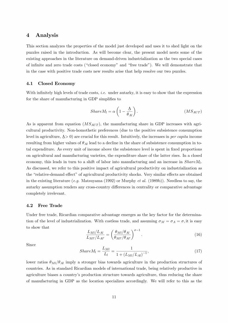
4.1 Closed Economy

With infinitely high levels of trade costs, i.e. under autarky, it is easy to show that the expression

for the share of manufacturing in GDP simplifies to

ShareMl = α

(1− A

¯θAl

). (MSAUT )

As is apparent from equation (MSAUT ), the manufacturing share in GDP increases with agri-

cultural productivity. Non-homothetic preferences (due to the positive subsistence consumption

level in agriculture, A¯> 0) are crucial for this result. Intuitively, the increases in per capita income

resulting from higher values of θAl lead to a decline in the share of subsistence consumption in to-

tal expenditure. As every unit of income above the subsistence level is spent in fixed proportions

on agricultural and manufacturing varieties, the expenditure share of the latter rises. In a closed

economy, this leads in turn to a shift of labor into manufacturing and an increase in ShareMl.

As discussed, we refer to this positive impact of agricultural productivity on industrialization as

the “relative-demand effect”of agricultural productivity shocks. Very similar effects are obtained

in the existing literature (e.g. Matsuyama (1992) or Murphy et al. (1989b)). Needless to say, the

autarky assumption renders any cross-country differences in centrality or comparative advantage

completely irrelevant.

4.2 Free Trade

Under free trade, Ricardian comparative advantage emerges as the key factor for the determina-

tion of the level of industrialization. With costless trade, and assuming σM = σA = σ, it is easy

to show thatLMl/LAlLMl′/LAl′

=

(θMl/θAlθMl′/θAl′

)σ−1. (16)

Since

ShareMl =LMl

Ll=

1

1 + (LMl/LAl)−1 , (17)

lower ratios θMl/θAl imply a stronger bias towards agriculture in the production structures of

countries. As in standard Ricardian models of international trade, being relatively productive in

agriculture biases a country’s production structure towards agriculture, thus reducing the share

of manufacturing in GDP as the location specializes accordingly. We will refer to this as the

11

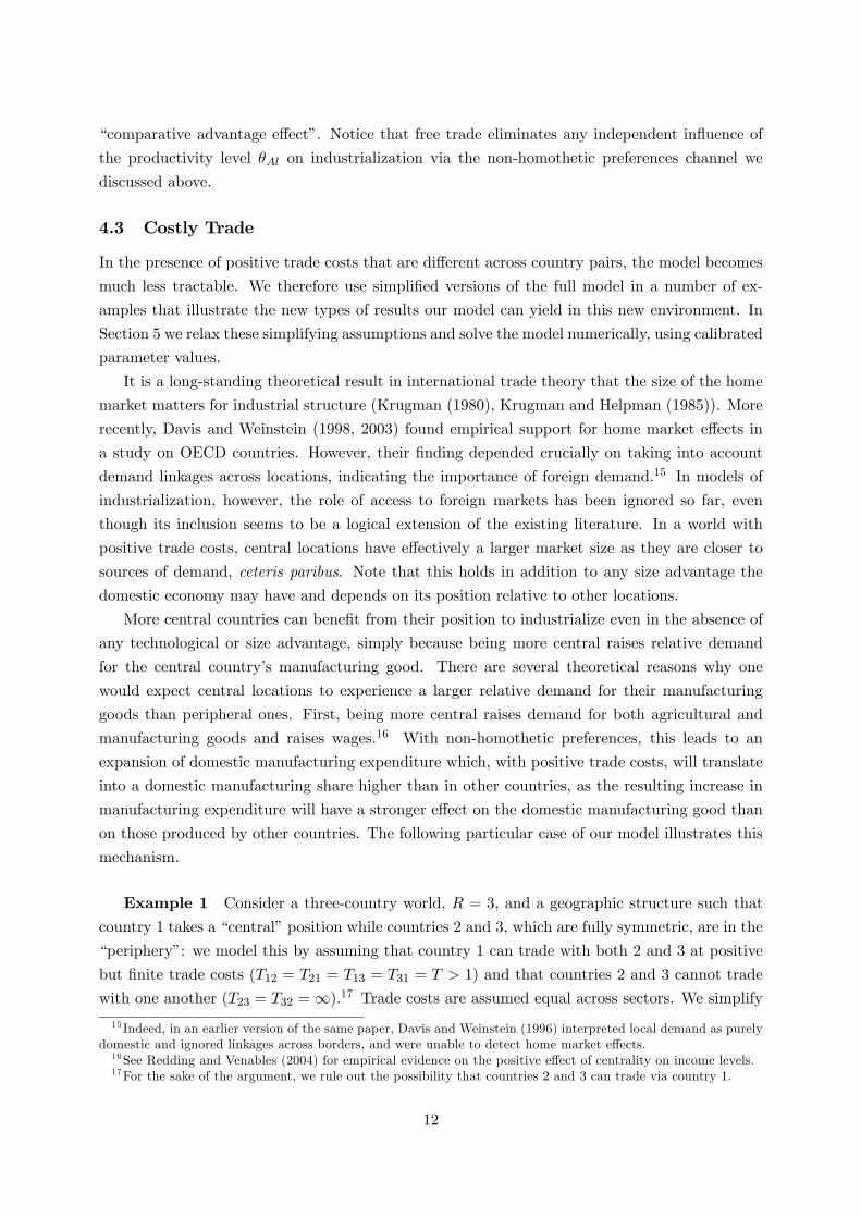
“comparative advantage effect”. Notice that free trade eliminates any independent influence of

the productivity level θAl on industrialization via the non-homothetic preferences channel we

discussed above.

4.3 Costly Trade

In the presence of positive trade costs that are different across country pairs, the model becomes

much less tractable. We therefore use simplified versions of the full model in a number of ex-

amples that illustrate the new types of results our model can yield in this new environment. In

Section 5 we relax these simplifying assumptions and solve the model numerically, using calibrated

parameter values.

It is a long-standing theoretical result in international trade theory that the size of the home

market matters for industrial structure (Krugman (1980), Krugman and Helpman (1985)). More

recently, Davis and Weinstein (1998, 2003) found empirical support for home market effects in

a study on OECD countries. However, their finding depended crucially on taking into account

demand linkages across locations, indicating the importance of foreign demand.15 In models of

industrialization, however, the role of access to foreign markets has been ignored so far, even

though its inclusion seems to be a logical extension of the existing literature. In a world with

positive trade costs, central locations have effectively a larger market size as they are closer to

sources of demand, ceteris paribus. Note that this holds in addition to any size advantage the

domestic economy may have and depends on its position relative to other locations.

More central countries can benefit from their position to industrialize even in the absence of

any technological or size advantage, simply because being more central raises relative demand

for the central country’s manufacturing good. There are several theoretical reasons why one

would expect central locations to experience a larger relative demand for their manufacturing

goods than peripheral ones. First, being more central raises demand for both agricultural and

manufacturing goods and raises wages.16 With non-homothetic preferences, this leads to an

expansion of domestic manufacturing expenditure which, with positive trade costs, will translate

into a domestic manufacturing share higher than in other countries, as the resulting increase in

manufacturing expenditure will have a stronger effect on the domestic manufacturing good than

on those produced by other countries. The following particular case of our model illustrates this

mechanism.

Example 1 Consider a three-country world, R = 3, and a geographic structure such that

country 1 takes a “central”position while countries 2 and 3, which are fully symmetric, are in the

“periphery”: we model this by assuming that country 1 can trade with both 2 and 3 at positive

but finite trade costs (T12 = T21 = T13 = T31 = T > 1) and that countries 2 and 3 cannot trade

with one another (T23 = T32 =∞).17 Trade costs are assumed equal across sectors. We simplify15 Indeed, in an earlier version of the same paper, Davis and Weinstein (1996) interpreted local demand as purely

domestic and ignored linkages across borders, and were unable to detect home market effects.16See Redding and Venables (2004) for empirical evidence on the positive effect of centrality on income levels.17For the sake of the argument, we rule out the possibility that countries 2 and 3 can trade via country 1.

12

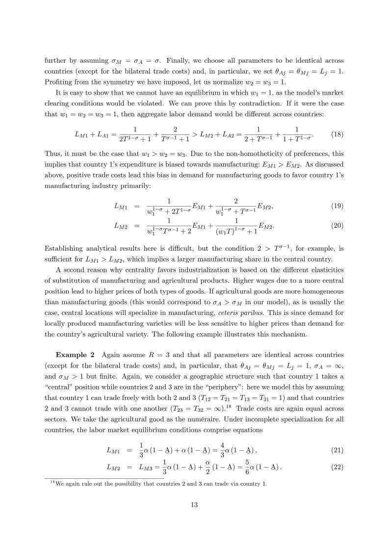
further by assuming σM = σA = σ. Finally, we choose all parameters to be identical across

countries (except for the bilateral trade costs) and, in particular, we set θAj = θMj = Lj = 1.

Profiting from the symmetry we have imposed, let us normalize w2 = w3 = 1.

It is easy to show that we cannot have an equilibrium in which w1 = 1, as the model’s market

clearing conditions would be violated. We can prove this by contradiction. If it were the case

that w1 = w2 = w3 = 1, then aggregate labor demand would be different across countries:

LM1 + LA1 =1

2T 1−σ + 1+

2

T σ−1 + 1> LM2 + LA2 =

1

2 + T σ−1+

1

1 + T 1−σ. (18)

Thus, it must be the case that w1 > w2 = w3. Due to the non-homotheticity of preferences, this

implies that country 1’s expenditure is biased towards manufacturing: EM1 > EM2. As discussed

above, positive trade costs lead this bias in demand for manufacturing goods to favor country 1’s

manufacturing industry primarily:

LM1 =1

w1−σ1 + 2T 1−σEM1 +

2

w1−σ1 + T σ−1EM2, (19)

LM2 =1

w1−σ1 T σ−1 + 2EM1 +

1

(w1T )1−σ + 1EM2. (20)

Establishing analytical results here is diffi cult, but the condition 2 > T σ−1, for example, is

suffi cient for LM1 > LM2, which implies a larger manufacturing share in the central country.

A second reason why centrality favors industrialization is based on the different elasticities

of substitution of manufacturing and agricultural products. Higher wages due to a more central

position lead to higher prices of both types of goods. If agricultural goods are more homogeneous

than manufacturing goods (this would correspond to σA > σM in our model), as is usually the

case, central locations will specialize in manufacturing, ceteris paribus. This is since demand for

locally produced manufacturing varieties will be less sensitive to higher prices than demand for

the country’s agricultural variety. The following example illustrates this mechanism.

Example 2 Again assume R = 3 and that all parameters are identical across countries

(except for the bilateral trade costs) and, in particular, that θAj = θMj = Lj = 1, σA = ∞,and σM > 1 but finite. Again, we consider a geographic structure such that country 1 takes a

“central”position while countries 2 and 3 are in the “periphery”: here we model this by assuming

that country 1 can trade freely with both 2 and 3 (T12 = T21 = T13 = T31 = 1) and that countries

2 and 3 cannot trade with one another (T23 = T32 = ∞).18 Trade costs are again equal acrosssectors. We take the agricultural good as the numéraire. Under incomplete specialization for all

countries, the labor market equilibrium conditions comprise equations

LM1 =1

3α (1−A

¯) + α (1−A

¯) =

4

3α (1−A

¯) , (21)

LM2 = LM3 =1

3α (1−A

¯) +

α

2(1−A

¯) =

5

6α (1−A

¯) . (22)

18We again rule out the possibility that countries 2 and 3 can trade via country 1.

13

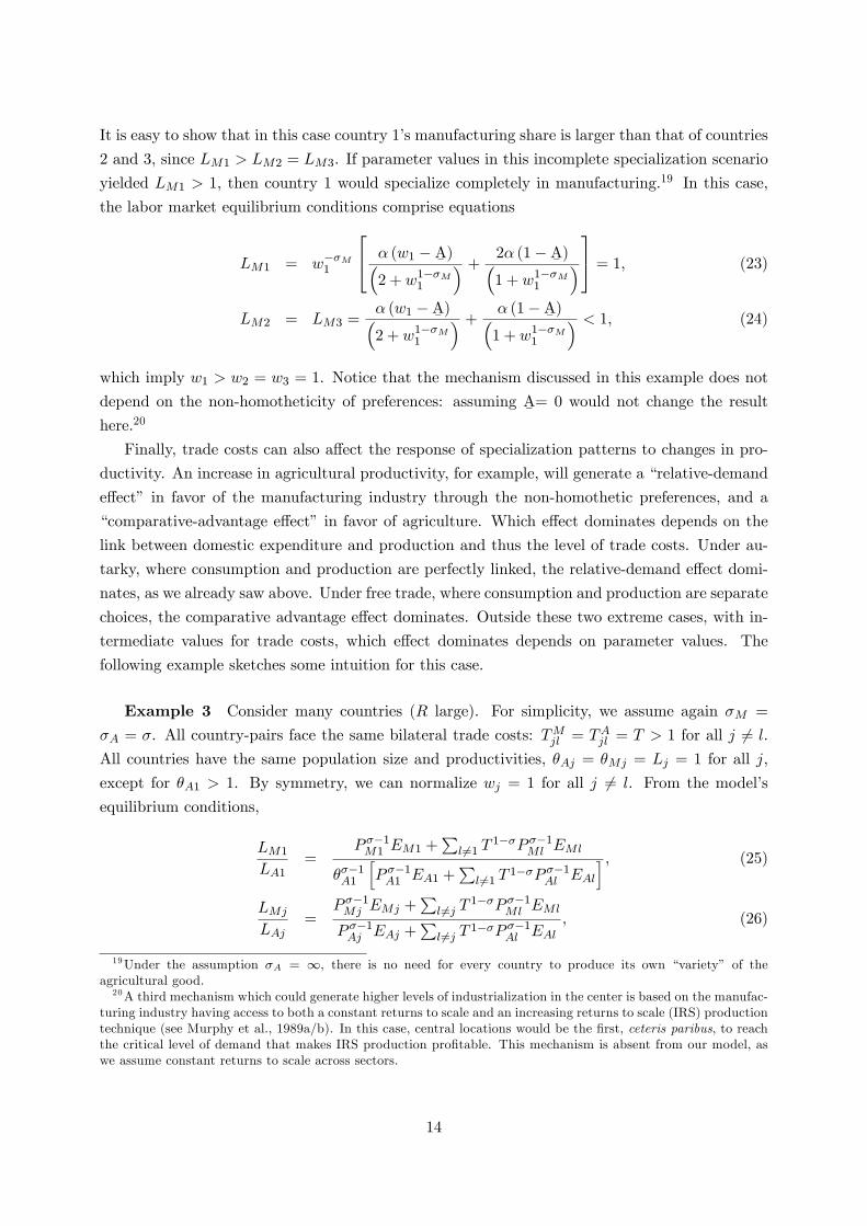
It is easy to show that in this case country 1’s manufacturing share is larger than that of countries

2 and 3, since LM1 > LM2 = LM3. If parameter values in this incomplete specialization scenario

yielded LM1 > 1, then country 1 would specialize completely in manufacturing.19 In this case,

the labor market equilibrium conditions comprise equations

LM1 = w−σM1

α (w1 −A¯ )(2 + w1−σM1

) +2α (1−A

¯)(

1 + w1−σM1

) = 1, (23)

LM2 = LM3 =α (w1 −A¯ )(2 + w1−σM1

) +α (1−A

¯)(

1 + w1−σM1

) < 1, (24)

which imply w1 > w2 = w3 = 1. Notice that the mechanism discussed in this example does not

depend on the non-homotheticity of preferences: assuming A¯

= 0 would not change the result

here.20

Finally, trade costs can also affect the response of specialization patterns to changes in pro-

ductivity. An increase in agricultural productivity, for example, will generate a “relative-demand

effect” in favor of the manufacturing industry through the non-homothetic preferences, and a

“comparative-advantage effect” in favor of agriculture. Which effect dominates depends on the

link between domestic expenditure and production and thus the level of trade costs. Under au-

tarky, where consumption and production are perfectly linked, the relative-demand effect domi-

nates, as we already saw above. Under free trade, where consumption and production are separate

choices, the comparative advantage effect dominates. Outside these two extreme cases, with in-

termediate values for trade costs, which effect dominates depends on parameter values. The

following example sketches some intuition for this case.

Example 3 Consider many countries (R large). For simplicity, we assume again σM =

σA = σ. All country-pairs face the same bilateral trade costs: TMjl = TAjl = T > 1 for all j 6= l.

All countries have the same population size and productivities, θAj = θMj = Lj = 1 for all j,

except for θA1 > 1. By symmetry, we can normalize wj = 1 for all j 6= l. From the model’s

equilibrium conditions,

LM1

LA1=

P σ−1M1 EM1 +∑

l 6=1 T1−σP σ−1Ml EMl

θσ−1A1

[P σ−1A1 EA1 +

∑l 6=1 T

1−σP σ−1Al EAl

] , (25)

LMj

LAj=

P σ−1Mj EMj +∑

l 6=j T1−σP σ−1Ml EMl

P σ−1Aj EAj +∑

l 6=j T1−σP σ−1Al EAl

, (26)

19Under the assumption σA = ∞, there is no need for every country to produce its own “variety” of theagricultural good.20A third mechanism which could generate higher levels of industrialization in the center is based on the manufac-

turing industry having access to both a constant returns to scale and an increasing returns to scale (IRS) productiontechnique (see Murphy et al., 1989a/b). In this case, central locations would be the first, ceteris paribus, to reachthe critical level of demand that makes IRS production profitable. This mechanism is absent from our model, aswe assume constant returns to scale across sectors.

14

for countries 1 and j. Assuming that trade costs are such that countries consume sizable amounts

of foreign goods, one can neglect the effect of θA1 on the price levels PMl and PAl. A high θA1therefore has a direct effect in the denominator of equation (25) and an indirect effect via a high

w1 in the terms EM1 and EA1 of both equations. Notice first that the direct effect of θA1 raises

country 1’s agricultural share in GDP (the comparative-advantage effect). Second, a higher w1(due to a higher θA1) tilts relative expenditure towards manufacturing in both country 1 and

country j because of the non-homotheticity in demand, but more so in country 1 due to the

presence of trade costs. As discussed above, this relative-demand effect operates in the direction

opposite to the comparative-advantage effect.

5 A Calibrated Multi-Country Model of Industrialization

The discussion in Section 4 has shown that our model is, in principle, able to replicate the stylized

facts from the introduction. However, our results relied on a number of simplifying assumptions

and may not generalize to the full model from Section 3 which, as discussed, does not have an

analytical solution. Also, the exact magnitude of parameter values mattered a great deal for the

direction of results, especially in example 3.

This is why we complement the analytical results with a full-scale multi-country calibration

of our model. That is, we ask to what extent the model matches our stylized facts for empirically

plausible parameter values. In the following, we choose parameters to match international trade

and expenditure data and use this calibrated model to generate data on manufacturing shares and

the independent variables used in the regressions in Tables 1 and 2 (more details on how exactly

this is done are provided below). Intuitively, if the true data generating process for our variables

of interest is similar to the one postulated by our model, we should expect to find comparable

multivariate correlations in both the real and the generated data.21

5.1 Parameter Values

For a calibrated version of our model, we need data on the size of countries’workforces (Ll) and

productivity levels (θAl, θMl), and values for the parameters governing substitution elasticities

(σA, σM ), trade costs (TAlj , TMlj ), the manufacturing expenditure share (α), and subsistence

consumption (A¯). Table 3 provides parameter estimates and a brief description of the calibration

procedure and data sources used. In the following, we describe the calibration in more detail.

Data requirements limit the sample to 107 countries for the year 2000, 79 of which are classified

21Note that we are not primarily interested in matching the cross-section of manufacturing shares and theindependent variables in Tables 1 and 2 as closely as possible, but only ask our model to reproduce (univariateand multivariate) correlations found in the real data. This is of course a strictly weaker test than trying to matchthe above variables exactly. (If we succeeded in doing so, we would naturally be able to reproduce the correlationsas well). To be sure, matching the entire distribution of the variables from Tables 1 and 2 is also interesting butwould require a yet more complicated model and is beyond the research objective of this paper (which, to reiterate,is to explain correlations in the data which are at odds with existing theories). Having said this, we provide someevidence below that the version of our model with positive but finite trade costs is actually more successful inmatching the cross-sectional variation in manufacturing shares than versions based on autarky or free trade.

15

as developing and will be used in our regression analysis of the simulated data.22

We follow Feenstra (1994) in using variation in import quantities and prices to identify elas-

ticities of substitution among manufacturing and agricultural varieties (σA, σM ). This approach,

as extended by Broda and Weinstein (2006) and Broda et al. (2006), has become the dominant

method for estimating substitution elasticities in the international trade literature in recent years.

In our setting, it has the additional advantage of building on a very similar demand structure as

our paper (CES and Armington varieties), while allowing for more general supply side features.

We adapt this approach to our setting by using data which correspond to our calibration exercise

in terms of country coverage, time period and the definition of sectors for which we estimate

elasticities. We focus on a discussion of our estimates in the following and refer the reader to

Appendix B for a more detailed description of the Feenstra-Broda-Weinstein methodology and

how we adapt it to our setting.

For our baseline elasticity estimates, we use cross-country trade data for the year 2000 but

restrict the estimation sample to the 102 countries which are in our calibration sample and for

which we have the necessary information on import prices and quantities.23 We obtain σM = 2.3

and σA = 2.3. For comparison, Broda et al. (2006) estimate elasticities of substitution between

varieties of goods produced in each of approximately 200 sectors, separately for 73 countries

(rather than imposing a common elasticity as we do in accordance with our model). The median

across these estimates for the 60 countries also present in our data is 3.4. Given the much higher

degree of aggregation in our data (two instead of 200 sectors), our lower estimates seem plausible.

This is because both economic theory and the empirical results of Broda and Weinstein (2006)

and Broda et al. (2006) suggest that estimated elasticities should fall as the level of aggregation

increases and varieties become less similar.24

As a robustness check, we also obtain estimates using data on imports by the U.S. from the

countries in our calibration sample.25 These data are likely to be of higher quality than the cross-

country data used before (see Feenstra, Romalis and Schott, 2002), although of course we only

have one importer now instead of 102. Using these data yields comparable coeffi cient magnitudes

as before although agricultural varities are now estimated to be slightly more substitutable across

countries (σM = 2.0 and σA = 2.6).

Since labor is the only factor of production in our model, we proxy θMl and θAl by labor

productivity in manufacturing and agriculture, respectively. However, as already briefly discussed

in Section 2, the cross-sectional variation in labor productivity across countries which we observe

22See Appendix A for a list of countries included in the calibration sample. All 107 countries will be used togenerate our synthetic data set as developed countries do of course play a major role in determining manufacturingshares and centrality of developing countries.23Three groups of countries only report one common set of trade data, explaining the five missing observations:

Botswana, Lesotho, Namibia and South Africa; Belgium and Luxembourg; and St. Lucia and St. Vincent and theGrenadines.24Closer to our level of aggregation but obtained via a different methodology is the estimate by Eaton et al.

(2008) who use French firm-level data to estimate an elasticity of substitution between individual manufacturingvarieties of σM = 1.7.25Again, we lose five countries due to aggregation in the trade data (see footnote 23), leaving us with 101

exporters (the U.S. is of course excluded as an exporter).

16

in the data is driven by both differences in technological effi ciency and differences in prices. That

is, lp.l = V A.l/L.l = p.lx.l/L.l in terms of our model because we abstract from intermediate

inputs. Since we are only interested in θ.l = x.l/L.l, we use data on purchasing power parities for

agriculture and manufacturing goods consumption from the International Comparison Program

(ICP) to construct proxies for p.l and strip out price variation from the data (see Appendix C for

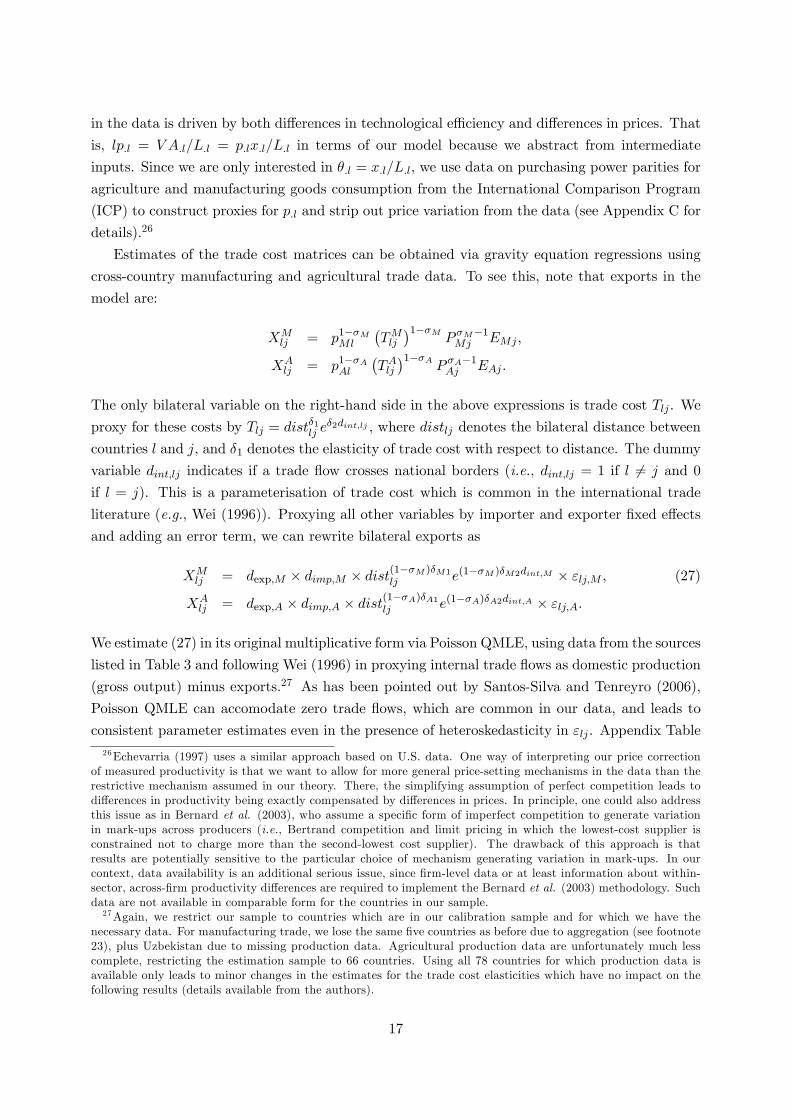
details).26

Estimates of the trade cost matrices can be obtained via gravity equation regressions using

cross-country manufacturing and agricultural trade data. To see this, note that exports in the

model are:

XMlj = p1−σMMl

(TMlj

)1−σMP σM−1Mj EMj ,

XAlj = p1−σAAl

(TAlj)1−σA

P σA−1Aj EAj .

The only bilateral variable on the right-hand side in the above expressions is trade cost Tlj . We

proxy for these costs by Tlj = distδ1lj eδ2dint,lj , where distlj denotes the bilateral distance between

countries l and j, and δ1 denotes the elasticity of trade cost with respect to distance. The dummy

variable dint,lj indicates if a trade flow crosses national borders (i.e., dint,lj = 1 if l 6= j and 0

if l = j). This is a parameterisation of trade cost which is common in the international trade

literature (e.g., Wei (1996)). Proxying all other variables by importer and exporter fixed effects

and adding an error term, we can rewrite bilateral exports as

XMlj = dexp,M × dimp,M × dist(1−σM )δM1

lj e(1−σM )δM2dint,M × εlj,M , (27)

XAlj = dexp,A × dimp,A × dist(1−σA)δA1lj e(1−σA)δA2dint,A × εlj,A.

We estimate (27) in its original multiplicative form via Poisson QMLE, using data from the sources

listed in Table 3 and following Wei (1996) in proxying internal trade flows as domestic production

(gross output) minus exports.27 As has been pointed out by Santos-Silva and Tenreyro (2006),

Poisson QMLE can accomodate zero trade flows, which are common in our data, and leads to

consistent parameter estimates even in the presence of heteroskedasticity in εlj . Appendix Table26Echevarria (1997) uses a similar approach based on U.S. data. One way of interpreting our price correction

of measured productivity is that we want to allow for more general price-setting mechanisms in the data than therestrictive mechanism assumed in our theory. There, the simplifying assumption of perfect competition leads todifferences in productivity being exactly compensated by differences in prices. In principle, one could also addressthis issue as in Bernard et al. (2003), who assume a specific form of imperfect competition to generate variationin mark-ups across producers (i.e., Bertrand competition and limit pricing in which the lowest-cost supplier isconstrained not to charge more than the second-lowest cost supplier). The drawback of this approach is thatresults are potentially sensitive to the particular choice of mechanism generating variation in mark-ups. In ourcontext, data availability is an additional serious issue, since firm-level data or at least information about within-sector, across-firm productivity differences are required to implement the Bernard et al. (2003) methodology. Suchdata are not available in comparable form for the countries in our sample.27Again, we restrict our sample to countries which are in our calibration sample and for which we have the

necessary data. For manufacturing trade, we lose the same five countries as before due to aggregation (see footnote23), plus Uzbekistan due to missing production data. Agricultural production data are unfortunately much lesscomplete, restricting the estimation sample to 66 countries. Using all 78 countries for which production data isavailable only leads to minor changes in the estimates for the trade cost elasticities which have no impact on thefollowing results (details available from the authors).

17

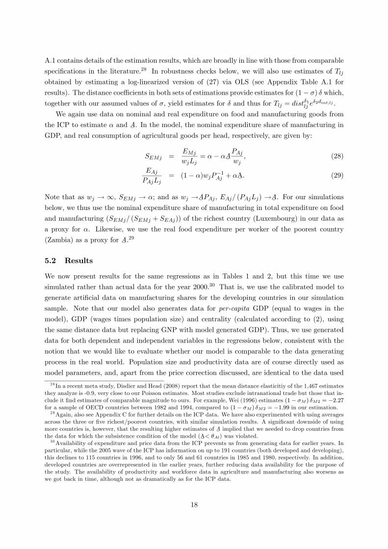
A.1 contains details of the estimation results, which are broadly in line with those from comparable

specifications in the literature.28 In robustness checks below, we will also use estimates of Tljobtained by estimating a log-linearized version of (27) via OLS (see Appendix Table A.1 for

results). The distance coeffi cients in both sets of estimations provide estimates for (1− σ) δ which,

together with our assumed values of σ, yield estimates for δ and thus for Tlj = distδ1lj eδ2dint,lj .

We again use data on nominal and real expenditure on food and manufacturing goods from

the ICP to estimate α and A¯. In the model, the nominal expenditure share of manufacturing in

GDP, and real consumption of agricultural goods per head, respectively, are given by:

SEMj =EMj

wjLj= α− αA

¯PAjwj

, (28)

EAjPAjLj

= (1− α)wjP−1Aj + αA

¯. (29)

Note that as wj → ∞, SEMj → α; and as wj →A¯ PAj , EAj/ (PAjLj) →A¯ . For our simulationsbelow, we thus use the nominal expenditure share of manufacturing in total expenditure on food

and manufacturing (SEMj/ (SEMj + SEAj)) of the richest country (Luxembourg) in our data as

a proxy for α. Likewise, we use the real food expenditure per worker of the poorest country

(Zambia) as a proxy for A¯.29

5.2 Results

We now present results for the same regressions as in Tables 1 and 2, but this time we use

simulated rather than actual data for the year 2000.30 That is, we use the calibrated model to

generate artificial data on manufacturing shares for the developing countries in our simulation

sample. Note that our model also generates data for per-capita GDP (equal to wages in the

model), GDP (wages times population size) and centrality (calculated according to (2), using

the same distance data but replacing GNP with model generated GDP). Thus, we use generated

data for both dependent and independent variables in the regressions below, consistent with the

notion that we would like to evaluate whether our model is comparable to the data generating

process in the real world. Population size and productivity data are of course directly used as

model parameters, and, apart from the price correction discussed, are identical to the data used

28 In a recent meta study, Disdier and Head (2008) report that the mean distance elasticitiy of the 1,467 estimatesthey analyze is -0.9, very close to our Poisson estimates. Most studies exclude intranational trade but those that in-clude it find estimates of comparable magnitude to ours. For example, Wei (1996) estimates (1− σM ) δM2 = −2.27for a sample of OECD countries between 1982 and 1994, compared to (1− σM ) δM2 = −1.99 in our estimation.29Again, also see Appendix C for further details on the ICP data. We have also experimented with using averages

across the three or five richest/poorest countries, with similar simulation results. A significant downside of usingmore countries is, however, that the resulting higher estimates of A

¯implied that we needed to drop countries from

the data for which the subsistence condition of the model (A¯< θAl) was violated.

30Availability of expenditure and price data from the ICP prevents us from generating data for earlier years. Inparticular, while the 2005 wave of the ICP has information on up to 191 countries (both developed and developing),this declines to 115 countries in 1996, and to only 56 and 61 countries in 1985 and 1980, respectively. In addition,developed countries are overrepresented in the earlier years, further reducing data availability for the purpose ofthe study. The availability of productivity and workforce data in agriculture and manufacturing also worsens aswe got back in time, although not as dramatically as for the ICP data.

18

in the regressions from Section 2.31

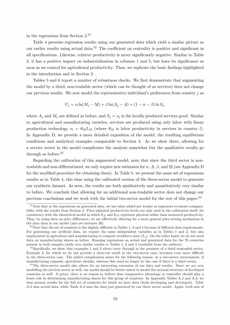
Table 4 presents regression results using our generated data which yield a similar picture as

our earlier results using actual data.32 The coeffi cient on centrality is positive and significant in

all specifications. Likewise, relative productivity is never significantly negative. Similar to Table

2, it has a positive impact on industrialization in columns 1 and 5, but loses its significance as

soon as we control for agricultural productivity. Thus, we replicate the basic findings highlighted

in the introduction and in Section 2.

Tables 5 and 6 report a number of robustness checks. We first demonstrate that augmenting

the model by a third, non-tradable sector (which can be thought of as services) does not change

our previous results. We now model the representative individual’s preferences from country j as

Uj = α ln(Mj −M¯ ) + β ln(Aj −A¯ ) + (1− α− β) lnSj ,

where Aj andMj are defined as before, and Sj = sj is the locally produced services good. Similar

to agricultural and manufacturing varieties, services are produced using only labor with linear

production technology sl = θSlLSl (where θSl is labor productivity in services in country l).

In Appendix D, we provide a more detailed exposition of the model, the resulting equilibrium

conditions and analytical examples comparable to Section 4. As we show there, allowing for

a service sector in the model complicates the analysis somewhat but the qualitative results go

through as before.33

Regarding the calibration of this augmented model, note that since the third sector is non-

tradable and non-differentiated, we only require new estimates for α, A¯, β, and M

¯(see Appendix D

for the modified procedure for obtaining them). In Table 5, we present the same set of regressions

results as in Table 4, this time using the calibrated version of the three-sector model to generate

our synthetic dataset. As seen, the results are both qualitatively and quantitatively very similar

to before. We conclude that allowing for an additional non-tradable sector does not change our

previous conclusions and we work with the initial two-sector model for the rest of this paper.34

31Note that in the regressions on generated data, we use value added per worker as regressors to ensure compara-bility with the results from Section 2. Price-adjusted productivity levels are only used in the calibration itself, forconsistency with the theoretical model in which θAl and θMl represent physical rather than measured productivity.Thus, by using data on price differences, we are effectively allowing for a more general price-setting mechanism inthe data than in our model (also see footnote 26).32Note that the set of countries is the slightly different in Tables 1, 2 and 4 because of different data requirements.

For generating our artificial data, we require the same independent variables as in Tables 1 and 2, but alsoemployment in agriculture and manufacturing to compute workforce sizes (Lj). On the other hand, we do not needdata on manufacturing shares as before. Running regressions on actual and generated data for the 76 countriespresent in both samples yields very similar results to Tables 1, 2 and 4 (available from the authors).33Specifically, we show that examples 1 and 2 above carry through in the presence of a third nontraded sector.

Example 3, for which we do not provide a clear-cut result in the two-sector case, becomes even more diffi cultin the three-sector case. The added complication arises for the following reason: in a two-sector environment, ifmanufacturing expands, agriculture shrinks, whereas this need no longer be the case if there is a third sector.34The three-sector model also allows for an interesting extension of our data and results. Since we are now

modelling the services sector as well, our model should be better suited to model the sectoral structure of developedcountries as well. A priori, there is no reason to believe that comparative advantage or centrality should play alesser role in determining manufacturing shares for this group of countries. In Appendix Tables A.2 and A.3, wethus present results for the full set of countries for which we have data (both developing and developed). TableA.2 uses actual data, while Table A.3 uses the data just generated by our three sector model. Again, both sets of

19

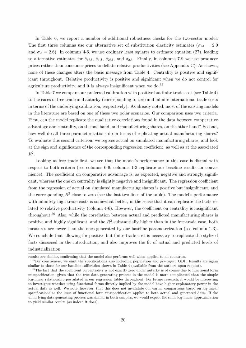
In Table 6, we report a number of additional robustness checks for the two-sector model.

The first three columns use our alternative set of substitution elasticity estimates (σM = 2.0

and σA = 2.6). In columns 4-6, we use ordinary least squares to estimate equation (27), leading

to alternative estimates for δ1M , δ1A, δ2M , and δ2A. Finally, in columns 7-9 we use producer

prices rather than consumer prices to deflate relative productivities (see Appendix C). As shown,

none of these changes alters the basic message from Table 4. Centrality is positive and signif-

icant throughout. Relative productivity is positive and significant when we do not control for

agriculture productivity, and it is always insignificant when we do.35

In Table 7 we compare our preferred calibration with positive but finite trade cost (see Table 4)

to the cases of free trade and autarky (corresponding to zero and infinite international trade costs

in terms of the underlying calibration, respectively). As already noted, most of the existing models

in the literature are based on one of these two polar scenarios. Our comparison uses two criteria.

First, can the model replicate the qualitative correlations found in the data between comparative

advantage and centrality, on the one hand, and manufacturing shares, on the other hand? Second,

how well do all three parameterizations do in terms of replicating actual manufacturing shares?

To evaluate this second criterion, we regress actual on simulated manufacturing shares, and look

at the sign and significance of the corresponding regression coeffi cient, as well as at the associated

R2.

Looking at free trade first, we see that the model’s performance in this case is dismal with

respect to both criteria (see columns 6-9; columns 1-3 replicate our baseline results for conve-

nience). The coeffi cient on comparative advantage is, as expected, negative and strongly signifi-

cant, whereas the one on centrality is slightly negative and insignificant. The regression coeffi cient

from the regression of actual on simulated manufacturing shares is positive but insignificant, and

the corresponding R2 close to zero (see the last two lines of the table). The model’s performance

with infinitely high trade costs is somewhat better, in the sense that it can replicate the facts re-

lated to relative productivity (column 4-6). However, the coeffi cient on centrality is insignificant

throughout.36 Also, while the correlation between actual and predicted manufacturing shares is

positive and highly significant, and the R2 substantially higher than in the free-trade case, both

measures are lower than the ones generated by our baseline parameterization (see column 1-3).

We conclude that allowing for positive but finite trade cost is necessary to replicate the stylized

facts discussed in the introduction, and also improves the fit of actual and predicted levels of

industrialization.

results are similar, confirming that the model also performs well when applied to all countries.35For conciseness, we omit the specifications also including population and per-capita GDP. Results are again

similar to those for our baseline calibration shown in Table 4 (available from the authors upon request).36The fact that the coeffi cient on centrality is not exactly zero under autarky is of course due to functional form

misspecification, given that the true data generating process in the model is more complicated than the simplelog-linear relationship postulated in our regression tables throughout. For future research, it would be interestingto investigate whether using functional forms directly implied by the model have higher explanatory power in theactual data as well. We note, however, that this does not invalidate our earlier comparisons based on log-linearspecifications as the issue of functional form misspecification applies to both actual and generated data. If theunderlying data generating process was similar in both samples, we would expect the same log-linear approximationto yield similar results (as indeed it does).

20

6 Conclusion

In this paper, we have drawn attention to two cross-sectional facts which, taken together, are

not easily explained by existing models of models of industrialization. First, proximity to foreign

sources of demand seems to matter for levels of industrialization. That is, there is a positive

correlation between manufacturing shares and the ‘centrality’of a country, i.e. its closeness to

foreign markets for its products. By construction, closed-economy models of industrialization

are not suited to explain this fact. We also noted that measures of centrality have substantial

explanatory power, explaining a comparable share of the cross-country variation in manufacturing

shares as one of the central explanatory variables in the literature, per-capita income.

While our first stylized fact seems to point to the importance of open-economy models, our

second fact suggests the opposite. Specifically, a standard proxy for Ricardian comparative

advantage in agriculture (labor productivity in agriculture relative to manufacturing) is not or

even positively correlated with manufacturing shares. This contradicts key predictions of open-

economy models which predict that countries integrated through trade should specialize according

to their comparative advantages.

We have argued that to understand these facts, we need to move beyond the closed-versus-

open-economy dichotomy prevalent in the literature, and to consider multi-country settings in

which countries interact with each other through international trade, but in which this interaction

is partly hampered by the fact that trade is not costless. We constructed a simple model along

these lines and used analytical examples and a full-scale multi-country calibration to show that

it can replicate our stylized facts.

References

[1] Bernard, A.B., J. Eaton, J.B. Jensen, and S. Kortum (2003): “Plants and Productivity in

International Trade,”American Economic Review, 93(4), 1268-1290.

[2] Breinlich, H. (2006): “The Spatial Income Structure in the European Union —What Role

for Economic Geography?,”Journal of Economic Geography, Nov. 2006, Vol. 6, No. 5.

[3] Broda, C., J. Greenfield, and D.E. Weinstein (2006): “From Groundnuts to Globalization:

A Structural Estimate of Trade and Growth,”NBER Working Paper 13041.

[4] Broda, C. and D.E. Weinstein (2006): “Globalization and the Gains from Variety,”Quarterly

Journal of Economics, Volume 121, Issue 2, May.

[5] Caselli, F. and Coleman, W.J. (2001): “The U.S. Structural Transformation and Regional

Convergence: A Reinterpretation,”Journal of Political Economy, 109, 584-616.

21

[6] Crafts, N. F. R. (1980): “Income Elasticities of Demand and the Release of Labor by Agri-

culture during the British Industrial Revolution: A further appraisal,”Journal of European

Economic History, 9, 153-168.

[7] Davis, Donald R. (1998): “The Home Market, Trade, and Industrial Structure,”American

Economic Review, 88(5), 1264-1276.

[8] Davis, Donald R. and David E. Weinstein (1996): “Does Economic Geography Matter for

International Specialization?,”, NBER Working Paper 5706.

[9] Davis, Donald R. and David E. Weinstein (1998): “Market Access, Economic Geography

and Comparative Advantage: An Empirical Assessment,”NBER Working Paper 6787.

[10] Davis, Donald R. and David E. Weinstein (2003): “Market Access, Economic Geography, and

Comparative Advantage: An Empirical Test,”Journal of International Economics, 59(1), pp.

1-23.

[11] Deardorff, Alan V. (2004): “Local Comparative Advantage: Trade Costs and the Pattern of

Trade”, Discussion Paper No. 500, University of Michigan.

[12] Disdier, Anne-Celia and Keith Head (2008): “The Puzzling Persistence of the Distance Effect

on Bilateral Trade,”Review of Economics and Statistics 90, 37-41.

[13] Eaton, J., S. Kortum and F. Kramarz (2008): “An Anatomy of International Trade: Evi-

dence from French Firms,”NBER Working Paper No. 14610.

[14] Echevarria, Christina (1997): “Changes in Sectoral Composition Associated with Economic

Growth,”International Economic Review, 38(2), 431-452.

[15] Feenstra, R. (1994): “New Product Varieties and the Measurement of International Prices,”

American Economic Review, 84(1), 157-177.

[16] Feenstra, R., J. Romalis, and P. Schott (2002): “U.S. Imports, Exports and Tariff Data,

1989-2001,”mimeo, University of California, Davis.

[17] Feenstra, R., R. Lipsey, H. Deng, A. Ma, and H. Mo (2005): “World Trade Flows, 1962-

2000,”NBER Working Paper 11040.

[18] Galor, O. and D. Weil (2000): “Population, Technology, and Growth: From Malthusian

Stagnation to the Demographic Transition and Beyond,”American Economic Review, 90,

806-828.

[19] Golub, Stephen S. and Hsieh, Chang-Tai (2000): “Classical Ricardian Theory of Comparative

Advantage Revisited,”Review of International Economics, 8(2), 221-234.

[20] Goodfriend, M. and J. McDermott (1995): “Early Development,”American Economic Re-

view 85, 116-133.

22

[21] Hanson, G. and C. Xiang (2004): “The Home Market Effect and Bilateral Trade Patterns,”

American Economic Review, 94 (4), pp. 1108-1129.

[22] Harris, J. (1954): “The market as a factor in the localization of industry in the United

States”Annals of the Association of American Geographers, 64, 315-348.

[23] Head, K. and T. Mayer (2006): “Regional Wage and Employment Responses to Market

Potential in the EU,”Regional Science and Urban Economics 36(5), 573-595.

[24] Kongsamut, P., S. Rebelo and D. Xie (2001): “Beyond Balanced Growth,”Review of Eco-

nomic Studies, 68, 869-882.

[25] Krugman, Paul R. (1980): “Scale Economies, Product Differentiation, and the Pattern of

Trade,”American Economic Review, 70, 950-959.

[26] Krugman, Paul R. and E. Helpman (1985): “Market Structure and Foreign Trade,”MIT

Press, Cambridge, MA.

[27] Laitner, John (2000): “Structural Change and Economic Growth,” Review of Economic

Studies, 67, 545-561.

[28] Leamer, Edward E. (1987): “Paths of Development in the Three-factor, n-good General

Equilibrium Model,”Journal of Political Economy, 95(5), 961-999.

[29] Matsuyama, K. (1992): “Agricultural Productivity, Comparative Advantage, and Economic

Growth,”Journal of Economic Theory, 58, 317-334.

[30] Matsuyama, K. (2009): “Structural Change in an Interdependent World: A Global View

of Manufacturing Decline,” Journal of the European Economic Association, Papers and

Proceedings.

[31] Murphy, Kevin M., A. Shleifer and R.V. Vishny (1989a): “Industrialization and the Big

Push,”Journal of Political Economy, 97(5), 1003-1026.

[32] Murphy, Kevin M., A. Shleifer and R.V. Vishny (1989b): “Income Distribution, Market Size,

and Industrialization,”Quarterly Journal of Economics, 104(3), 537-564.

[33] Ngai, L.R. and C.A. Pissarides (2007): “Structural Change in a Multisector Model of

Growth,”American Economic Review, 97, 429-443.

[34] Parente, Stephen L. and Edward C. Prescott (1994): “Barriers to Technology Adoption and

Development,”Journal of Political Economy, 102, 298-321.

[35] Parente, Stephen L. and Edward C. Prescott (2000): “Barriers to Riches,” MIT Press,

Cambridge, MA.

[36] Puga, D. and A.J. Venables (1996): “The spread of industry: spatial agglomeration in

economic development,”Journal of the Japanese and International Economy, 10, 440-464.

23

[37] Puga, D. and A.J. Venables (1999): “Agglomeration and Economic Development: Import

Substitution vs. Trade Liberalisation,”Economic Journal, 109, 292-311.

[38] Redding, S. and A.J. Venables (2004): “Economic Geography and International Inequality,”

Journal of International Economics, 62, 53-82.

[39] Rosenstein-Rodan, Paul N. (1943): “Problems of Industrialization of Eastern and South-

Eastern Europe,”Economic Journal, 53, 202-211.

[40] Santos-Silva, João M.C. and Silvana Tenreyro (2005): “The Log of Gravity,” Review of

Economics and Statistics, 88, 641-658.

[41] Schott, P. (2003): “One Size Fits All? Heckscher-Ohlin Specialization in Global Production,”

American Economic Review, 686-708.

[42] Syrquin, M. and H. Chenery (1989): “Patterns of Development, 1950 to 1983”, World Bank

Discussion Paper 41.

[43] Ventura, J. (1997): “Growth and interdependence,”Quarterly Journal of Economics, 112,

57-84.

[44] Wei, S.J. (1996): “Intra-National versus International Trade: How Stubborn are Nations in

Global Integration?,”NBER Working Paper 5531.

[45] Yi, K.M. and J. Zhang (2010): “Structural Change in an Open Economy,”mimeo, Federal

Reserve Bank of Philadelphia.

24

A Appendix A: Country Lists and Data used in Cross-CountryRegressions

Country List I - Cross-Country Regressions Albania (ALB); Algeria (DZA); Angola(AGO); Argentina (ARG); Armenia (ARM); Azerbaijan (AZE); Bangladesh (BGD); Barbados(BRB); Belarus (BLR); Belize (BLZ); Benin (BEN); Bhutan (BTN); Bolivia (BOL); Botswana(BWA); Brazil (BRA); Bulgaria (BGR); Burkina Faso (BFA); Burundi (BDI); Cambodia (KHM);Cameroon (CMR); Cape Verde (CPV); Central African Republic (CAF); Chad (TCD); Chile(CHL); China (CHN); Colombia (COL); Comoros (COM); Congo, Dem. Rep. (ZAR); Congo,Rep. (COG); Costa Rica (CRI); Cote d’Ivoire (CIV); Croatia (HRV); Czech Republic (CZE);Dominican Republic (DOM); Ecuador (ECU); Egypt, Arab Rep. (EGY); El Salvador (SLV);Equatorial Guinea (GNQ); Eritrea (ERI); Estonia (EST); Ethiopia (ETH); Fiji (FJI); Gabon(GAB); Gambia, The (GMB); Georgia (GEO); Ghana (GHA); Grenada (GRD); Guatemala(GTM); Guinea (GIN); Guinea-Bissau (GNB); Guyana (GUY); Honduras (HND); Hungary(HUN); India (IND); Indonesia (IDM); Iran, Islamic Rep. (IRN); Jamaica (JAM); Jordan (JOR);Kazakhstan (KAZ); Kenya (KEN); Korea, Rep. (KOR); Kyrgyz Republic (KGZ); Lao PDR(LAO); Latvia (LVA); Lesotho (LSO); Lithuania (LTU); Macedonia, FYR (MKD); Madagas-car (MDG); Malawi (MWI); Malaysia (MYS); Mali (MLI); Mauritania (MRT); Mexico (MEX);Moldova (MDA); Mongolia (MNG); Morocco (MAR); Mozambique (MOZ); Namibia (NAM);Nepal (NPL); Nicaragua (NIC); Niger (NER); Nigeria (NGA); Oman (OMN); Pakistan (PAK);Panama (PAN); Papua New Guinea (PNG); Paraguay (PRY); Peru (PER); Philippines (PHL);Poland (POL); Romania (ROM); Rwanda (RWA); Saudi Arabia (SAU); Senegal (SEN); SierraLeone (SLE); Slovak Republic (SVK); South Africa (ZAF); Sri Lanka (LKA); St. Lucia (LCA);St. Vincent and the Grenadines (VCT); Sudan (SDN); Suriname (SUR); Syrian Arab Re-public (SYR); Tanzania (TZA); Thailand (THA); Togo (TGO); Trinidad and Tobago (TTO);Tunisia (TUN); Turkey (TUR); Uganda (UGA); Ukraine (UKR); Uruguay (URY); Uzbekistan(UZB); Venezuela, RB (VEN); Vietnam (VNM); Yemen, Rep. (YEM); Zambia (ZMB); Zimbabwe(ZWE).

Country List II - Calibration Sample Developing countries: Albania (ALB); Algeria(DZA); Argentina (ARG); Armenia (ARM); Azerbaijan (AZE); Bangladesh (BGD); Barbados(BRB); Belize (BLZ); Bolivia (BOL); Botswana (BWA); Brazil (BRA); Bulgaria (BGR); Cam-bodia (KHM); Cameroon (CMR); Chile (CHL); China (CHN); Colombia (COL); Costa Rica(CRI); Croatia (HRV); Czech Republic (CZE); Dominican Republic (DOM); Ecuador (ECU);Egypt, Arab Rep. (EGY); El Salvador (SLV); Estonia (EST); Georgia (GEO); Ghana (GHA);Guatemala (GTM); Guyana (GUY); Honduras (HND); Hungary (HUN); Indonesia (IDM); Ja-maica (JAM); Jordan (JOR); Kazakhstan (KAZ); Korea, Rep. (KOR); Kyrgyz Republic (KGZ);Latvia (LVA); Lesotho (LSO); Lithuania (LTU); Macedonia, FYR (MKD); Malaysia (MYS);Mexico (MEX); Moldova (MDA); Mongolia (MNG); Morocco (MAR); Namibia (NAM); Nepal(NPL); Nicaragua (NIC); Oman (OMN); Pakistan (PAK); Panama (PAN); Papua New Guinea(PNG); Paraguay (PRY); Peru (PER); Philippines (PHL); Poland (POL); Romania (ROM);Russian Federation (RUS); Saudi Arabia (SAU); Slovak Republic (SVK); South Africa (ZAF);Sri Lanka (LKA); St. Lucia (LCA); St. Vincent and the Grenadines (VCT); Suriname (SUR);Syrian Arab Republic (SYR); Tanzania (TZA); Thailand (THA); Trinidad and Tobago (TTO);Turkey (TUR); Ukraine (UKR); Uruguay (URY); Uzbekistan (UZB); Venezuela, RB (VEN);Vietnam (VNM); Yemen, Rep. (YEM); Zambia (ZMB); Zimbabwe (ZWE).

Developed countries: Australia (AUS); Austria (AUT); Belgium (BEL); Brunei Darus-salam (BRN); Canada (CAN); Cyprus (CYP); Denmark (DKF); Finland (FIN); France (FRA);

25

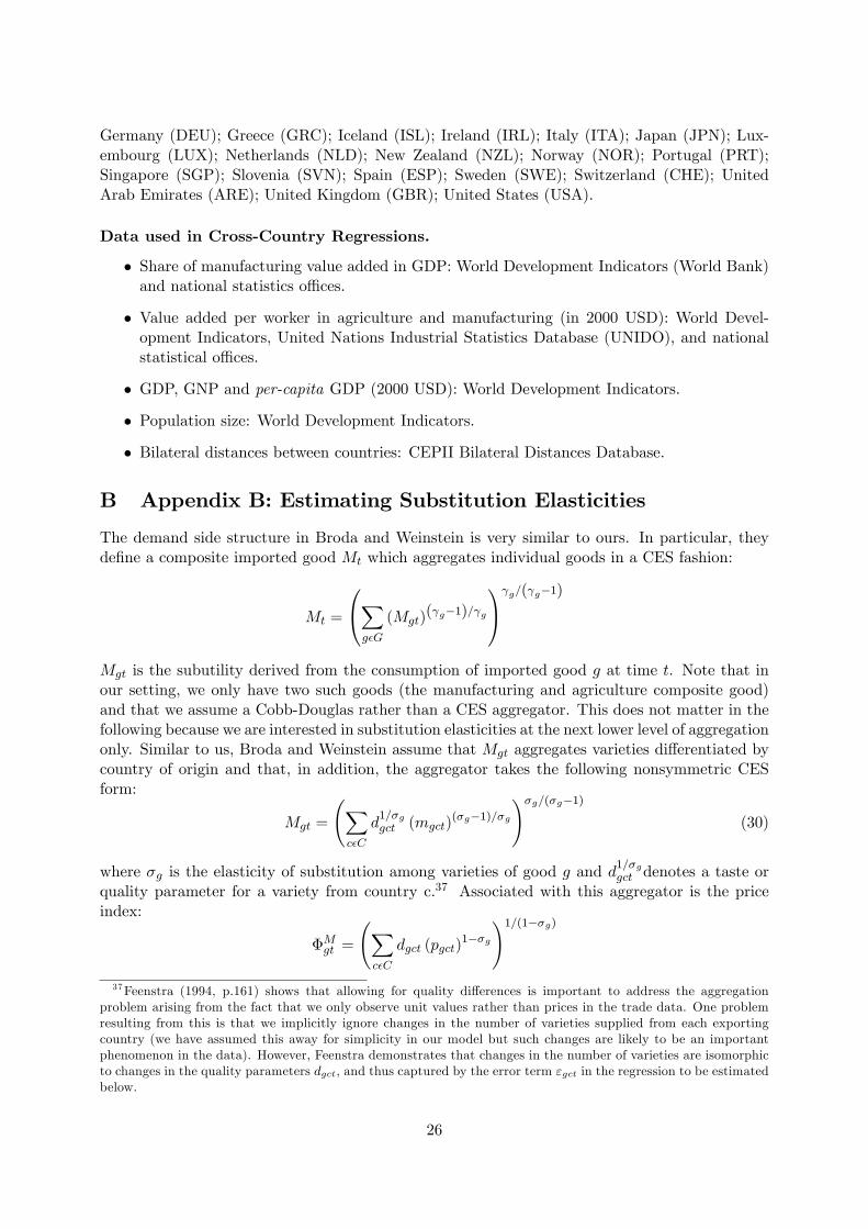
Germany (DEU); Greece (GRC); Iceland (ISL); Ireland (IRL); Italy (ITA); Japan (JPN); Lux-embourg (LUX); Netherlands (NLD); New Zealand (NZL); Norway (NOR); Portugal (PRT);Singapore (SGP); Slovenia (SVN); Spain (ESP); Sweden (SWE); Switzerland (CHE); UnitedArab Emirates (ARE); United Kingdom (GBR); United States (USA).

Data used in Cross-Country Regressions.

• Share of manufacturing value added in GDP: World Development Indicators (World Bank)and national statistics offi ces.

• Value added per worker in agriculture and manufacturing (in 2000 USD): World Devel-opment Indicators, United Nations Industrial Statistics Database (UNIDO), and nationalstatistical offi ces.

• GDP, GNP and per-capita GDP (2000 USD): World Development Indicators.

• Population size: World Development Indicators.

• Bilateral distances between countries: CEPII Bilateral Distances Database.

B Appendix B: Estimating Substitution Elasticities

The demand side structure in Broda and Weinstein is very similar to ours. In particular, theydefine a composite imported good Mt which aggregates individual goods in a CES fashion:

Mt =

∑gεG

(Mgt)(γg−1)/γg

γg/(γg−1)

Mgt is the subutility derived from the consumption of imported good g at time t. Note that inour setting, we only have two such goods (the manufacturing and agriculture composite good)and that we assume a Cobb-Douglas rather than a CES aggregator. This does not matter in thefollowing because we are interested in substitution elasticities at the next lower level of aggregationonly. Similar to us, Broda and Weinstein assume that Mgt aggregates varieties differentiated bycountry of origin and that, in addition, the aggregator takes the following nonsymmetric CESform:

Mgt =

(∑cεC

d1/σggct (mgct)

(σg−1)/σg

)σg/(σg−1)(30)

where σg is the elasticity of substitution among varieties of good g and d1/σggct denotes a taste or

quality parameter for a variety from country c.37 Associated with this aggregator is the priceindex:

ΦMgt =

(∑cεC

dgct (pgct)1−σg

)1/(1−σg)37Feenstra (1994, p.161) shows that allowing for quality differences is important to address the aggregation

problem arising from the fact that we only observe unit values rather than prices in the trade data. One problemresulting from this is that we implicitly ignore changes in the number of varieties supplied from each exportingcountry (we have assumed this away for simplicity in our model but such changes are likely to be an importantphenomenon in the data). However, Feenstra demonstrates that changes in the number of varieties are isomorphicto changes in the quality parameters dgct, and thus captured by the error term εgct in the regression to be estimatedbelow.

26

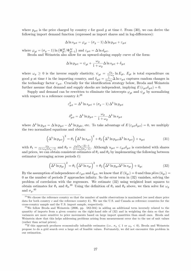
where pgct is the price charged by country c for good g at time t. From (30), we can derive thefollowing import demand function (expressed as import shares and in log-differences):

∆ ln sgct = ϕgt − (σg − 1) ∆ ln pgct + εgct

where ϕgt = (σg − 1) ln(ΦMgt /Φ

Mgt−1

)and εgct = ∆ ln dgct.

Broda and Weinstein also allow for an upward-sloping supply curve of the form:

∆ ln pgct = ψgt +ωg

1 + ωg∆ ln sgct + δgct

where ωg ≥ 0 is the inverse supply elasticity, ψgt =ωg1+ωg

lnEgt, Egt is total expenditure on

good g at time t in the importing country, and δgct = 11+ωg

∆ ln υgct captures random changes inthe technology factor υgct. Crucially for the identification strategy below, Broda and Weinsteinfurther assume that demand and supply shocks are independent, implying E (εgctδgct) = 0.

Supply and demand can be rewritten to eliminate the intercepts ϕgt and ψgt by normalizingwith respect to a reference country k:38

εkgct = ∆k ln sgct + (σg − 1) ∆k ln pgct

δkgct = ∆k ln pgct −ωg

1 + ωg∆k ln sgct

where ∆k ln pgct = ∆ ln pgct −∆k ln pgkt, etc. To take advantage of E (εgctδgct) = 0, we multiplythe two normalized equations and obtain:(

∆k ln pgct

)2= θ1

(∆k ln sgct

)2+ θ2

(∆k ln pgct∆

k ln sgct

)+ ugct (31)

with θ1 =ωg

(1+ωg)(σg−1) and θ2 =ωg(σg−2)−1(1+ωg)(σg−1) . Although ugct = εgctδgct is correlated with shares

and prices, we can obtain consistent estimates of θ1 and θ2 by implementing the following betweenestimator (averaging across periods t):(

∆k ln pgc

)2= θ1

(∆k ln sgc

)2+ θ2

(∆k ln pgc∆k ln sgc

)+ ugc (32)

By the assumption of independence of εgct and δgct, we know that E (ugc) = 0 and thus plim (ugc) =0 as the number of periods T approaches infinity. So the error term in (32) vanishes, solving theproblem of correlation with the regressors. We estimate (32) using weighted least squares toobtain estimates for θ1 and θ2.39 Using the definition of θ1 and θ2 above, we then solve for ωgand σg.40

38We choose the reference country so that the number of usable observations is maximised (we need share pricedata for both country c and the reference country k). We use the U.S. and Canada as reference countries for thecross-country sample and the U.S. import sample, respectively.39We follow Broda and Weinstein (2006, pp. 582-584) in adding an additional term inversely related to the

quantity of imports from a given country on the right-hand side of (32) and in weighting the data so that thevariances are more sensitive to price movements based on large import quantities than small ones. Broda andWeinstein show that this helps addressing problems arising from measurement error due to the use of unit values(rather than actual prices).40 If this approach produces economically infeasible estimates (i.e., σg ≤ 1 or ωg < 0), Broda and Weinstein

propose to do a grid search over a large set of feasible values. Fortunately, we did not encounter this problem inour estimation.

27

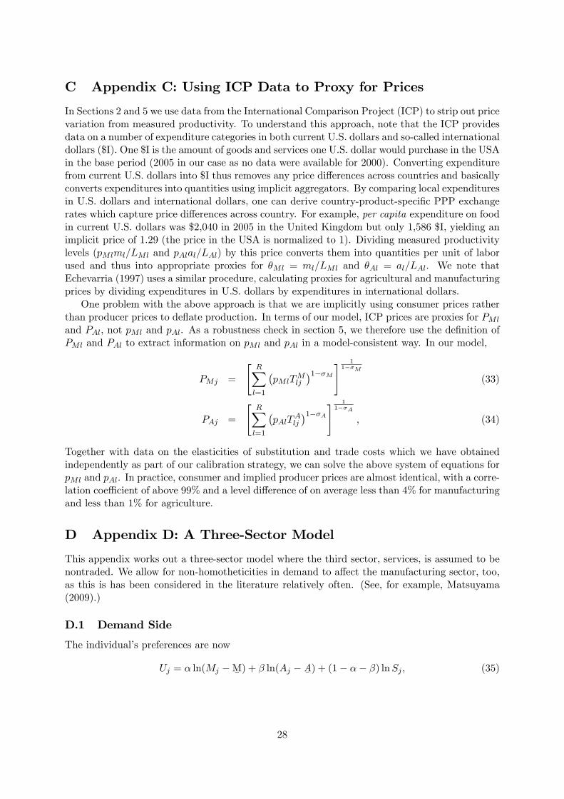
C Appendix C: Using ICP Data to Proxy for Prices

In Sections 2 and 5 we use data from the International Comparison Project (ICP) to strip out pricevariation from measured productivity. To understand this approach, note that the ICP providesdata on a number of expenditure categories in both current U.S. dollars and so-called internationaldollars ($I). One $I is the amount of goods and services one U.S. dollar would purchase in the USAin the base period (2005 in our case as no data were available for 2000). Converting expenditurefrom current U.S. dollars into $I thus removes any price differences across countries and basicallyconverts expenditures into quantities using implicit aggregators. By comparing local expendituresin U.S. dollars and international dollars, one can derive country-product-specific PPP exchangerates which capture price differences across country. For example, per capita expenditure on foodin current U.S. dollars was $2,040 in 2005 in the United Kingdom but only 1,586 $I, yielding animplicit price of 1.29 (the price in the USA is normalized to 1). Dividing measured productivitylevels (pMlml/LMl and pAlal/LAl) by this price converts them into quantities per unit of laborused and thus into appropriate proxies for θMl = ml/LMl and θAl = al/LAl. We note thatEchevarria (1997) uses a similar procedure, calculating proxies for agricultural and manufacturingprices by dividing expenditures in U.S. dollars by expenditures in international dollars.

One problem with the above approach is that we are implicitly using consumer prices ratherthan producer prices to deflate production. In terms of our model, ICP prices are proxies for PMl

and PAl, not pMl and pAl. As a robustness check in section 5, we therefore use the definition ofPMl and PAl to extract information on pMl and pAl in a model-consistent way. In our model,

PMj =

[R∑l=1

(pMlT

Mlj

)1−σM] 11−σM

(33)

PAj =

[R∑l=1

(pAlT

Alj

)1−σA] 11−σA

, (34)

Together with data on the elasticities of substitution and trade costs which we have obtainedindependently as part of our calibration strategy, we can solve the above system of equations forpMl and pAl. In practice, consumer and implied producer prices are almost identical, with a corre-lation coeffi cient of above 99% and a level difference of on average less than 4% for manufacturingand less than 1% for agriculture.

D Appendix D: A Three-Sector Model

This appendix works out a three-sector model where the third sector, services, is assumed to benontraded. We allow for non-homotheticities in demand to affect the manufacturing sector, too,as this is has been considered in the literature relatively often. (See, for example, Matsuyama(2009).)

D.1 Demand Side

The individual’s preferences are now

Uj = α ln(Mj −M¯ ) + β ln(Aj −A¯ ) + (1− α− β) lnSj , (35)

28

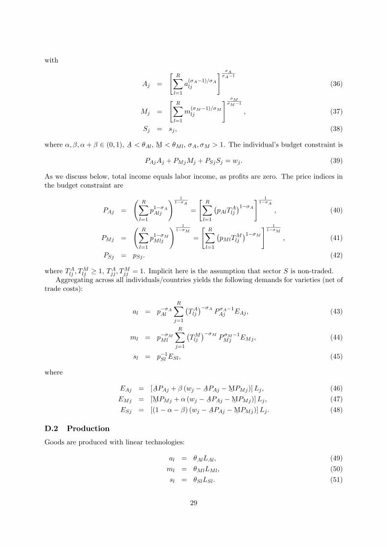
with

Aj =

[R∑l=1

a(σA−1)/σAlj

] σAσA−1

(36)

Mj =

[R∑l=1

m(σM−1)/σMlj

] σMσM−1

, (37)

Sj = sj , (38)

where α, β, α+ β ∈ (0, 1), A¯< θAl, M¯

< θMl, σA, σM > 1. The individual’s budget constraint is

PAjAj + PMjMj + PSjSj = wj . (39)

As we discuss below, total income equals labor income, as profits are zero. The price indices inthe budget constraint are

PAj =

(R∑l=1

p1−σAAlj

) 11−σA

=

[R∑l=1

(pAlT

Alj

)1−σA] 11−σA

, (40)

PMj =

(R∑l=1

p1−σMMlj

) 11−σM

=

[R∑l=1

(pMlT

Mlj

)1−σM] 11−σM

, (41)

PSj = pSj . (42)

where TAlj , TMlj ≥ 1, TAjj , T

Mjj = 1. Implicit here is the assumption that sector S is non-traded.

Aggregating across all individuals/countries yields the following demands for varieties (net oftrade costs):

al = p−σAAl

R∑j=1

(TAlj)−σA

P σA−1Aj EAj , (43)

ml = p−σMMl

R∑j=1

(TMlj

)−σMP σM−1Mj EMj , (44)

sl = p−1Sl ESl, (45)

where

EAj = [A¯PAj + β (wj −A¯ PAj −M¯ PMj)]Lj , (46)

EMj = [M¯PMj + α (wj −A¯ PAj −M¯ PMj)]Lj , (47)

ESj = [(1− α− β) (wj −A¯ PAj −M¯ PMj)]Lj . (48)

D.2 Production

Goods are produced with linear technologies:

al = θAlLAl, (49)

ml = θMlLMl, (50)

sl = θSlLSl. (51)

29

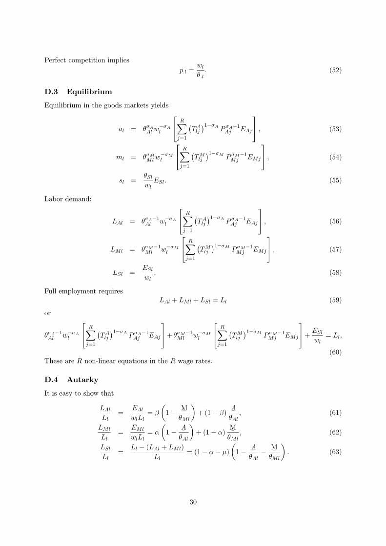
Perfect competition impliesp.l =

wlθ.l. (52)

D.3 Equilibrium

Equilibrium in the goods markets yields

al = θσAAl w−σAl

R∑j=1

(TAlj)1−σA

P σA−1Aj EAj

, (53)

ml = θσMMlw−σMl

R∑j=1

(TMlj

)1−σMP σM−1Mj EMj

, (54)

sl =θSlwlESl. (55)

Labor demand:

LAl = θσA−1Al w−σAl

R∑j=1

(TAlj)1−σA

P σA−1Aj EAj

, (56)

LMl = θσM−1Ml w−σMl

R∑j=1

(TMlj

)1−σMP σM−1Mj EMj

, (57)

LSl =ESlwl

. (58)

Full employment requiresLAl + LMl + LSl = Ll (59)

or

θσA−1Al w−σAl

R∑j=1

(TAlj)1−σA

P σA−1Aj EAj

+ θσM−1Ml w−σMl

R∑j=1

(TMlj

)1−σMP σM−1Mj EMj

+ESlwl

= Ll,

(60)These are R non-linear equations in the R wage rates.

D.4 Autarky

It is easy to show that

LAlLl

=EAlwlLl

= β

(1− M

¯θMl

)+ (1− β)

A¯θAl

, (61)

LMl

Ll=

EMl

wlLl= α

(1− A

¯θAl

)+ (1− α)

M¯θMl

, (62)

LSlLl

=Ll − (LAl + LMl)

Ll= (1− α− µ)

(1− A

¯θAl− M

¯θMl

). (63)

30

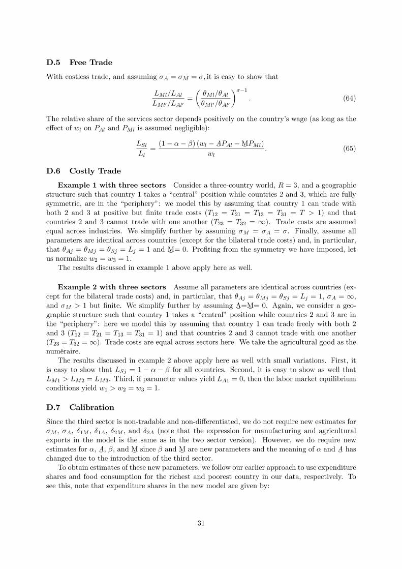
D.5 Free Trade

With costless trade, and assuming σA = σM = σ, it is easy to show that

LMl/LAlLMl′/LAl′

=

(θMl/θAlθMl′/θAl′

)σ−1. (64)

The relative share of the services sector depends positively on the country’s wage (as long as theeffect of wl on PAl and PMl is assumed negligible):

LSlLl

=(1− α− β) (wl −A¯ PAl −M¯ PMl)

wl. (65)

D.6 Costly Trade

Example 1 with three sectors Consider a three-country world, R = 3, and a geographicstructure such that country 1 takes a “central”position while countries 2 and 3, which are fullysymmetric, are in the “periphery”: we model this by assuming that country 1 can trade withboth 2 and 3 at positive but finite trade costs (T12 = T21 = T13 = T31 = T > 1) and thatcountries 2 and 3 cannot trade with one another (T23 = T32 = ∞). Trade costs are assumedequal across industries. We simplify further by assuming σM = σA = σ. Finally, assume allparameters are identical across countries (except for the bilateral trade costs) and, in particular,that θAj = θMj = θSj = Lj = 1 and M

¯= 0. Profiting from the symmetry we have imposed, let

us normalize w2 = w3 = 1.The results discussed in example 1 above apply here as well.

Example 2 with three sectors Assume all parameters are identical across countries (ex-cept for the bilateral trade costs) and, in particular, that θAj = θMj = θSj = Lj = 1, σA = ∞,and σM > 1 but finite. We simplify further by assuming A

¯=M¯

= 0. Again, we consider a geo-graphic structure such that country 1 takes a “central”position while countries 2 and 3 are inthe “periphery”: here we model this by assuming that country 1 can trade freely with both 2and 3 (T12 = T21 = T13 = T31 = 1) and that countries 2 and 3 cannot trade with one another(T23 = T32 =∞). Trade costs are equal across sectors here. We take the agricultural good as thenuméraire.

The results discussed in example 2 above apply here as well with small variations. First, itis easy to show that LSj = 1 − α − β for all countries. Second, it is easy to show as well thatLM1 > LM2 = LM3. Third, if parameter values yield LA1 = 0, then the labor market equilibriumconditions yield w1 > w2 = w3 = 1.

D.7 Calibration

Since the third sector is non-tradable and non-differentiated, we do not require new estimates forσM , σA, δ1M , δ1A, δ2M , and δ2A (note that the expression for manufacturing and agriculturalexports in the model is the same as in the two sector version). However, we do require newestimates for α, A

¯, β, and M

¯since β and M

¯are new parameters and the meaning of α and A

¯has

changed due to the introduction of the third sector.To obtain estimates of these new parameters, we follow our earlier approach to use expenditure

shares and food consumption for the richest and poorest country in our data, respectively. Tosee this, note that expenditure shares in the new model are given by:

31

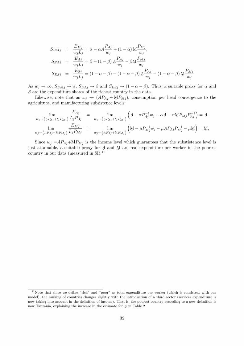
SEMj =EMj

wjLj= α− αA

¯PAjwj

+ (1− α)M¯PMj

wj,

SEAj =EAjwjLj

= β + (1− β)A¯PAjwj− βM

¯PMj

wj

SESj =ESjwjLj

= (1− α− β)− (1− α− β)A¯PAjwj− (1− α− β)M

¯PMj

wj

As wj → ∞, SEMj → α, SEAj → β and SESj → (1− α− β). Thus, a suitable proxy for α andβ are the expenditure shares of the richest country in the data.

Likewise, note that as wj → (A¯PAj +M

¯PMj), consumption per head convergence to the

agricultural and manufacturing subsistence levels:

limwj→(A

¯PAj+M¯

PMj)

EAjLjPAj

= limwj→(A

¯PAj+M¯

PMj)

(A¯

+ αP−1Aj wj − αA¯ − αM¯ PMjP−1Aj

)= A¯,

limwj→(A

¯PAj+M¯

PMj)

EMj

LjPMj= lim

wj→(A¯PAj+M¯

PMj)

(M¯

+ µP−1Mjwj − µA¯ PAjP−1Mj − µM¯

)= M¯,

Since wj =A¯PAj+M¯

PMj is the income level which guarantees that the substistence level isjust attainable, a suitable proxy for A

¯and M

¯are real expenditure per worker in the poorest

country in our data (measured in $I).41

41Note that since we define “rich” and “poor” as total expenditure per worker (which is consistent with ourmodel), the ranking of countries changes slightly with the introduction of a third sector (services expenditure isnow taking into account in the definition of income). That is, the poorest country according to a new definition isnow Tanzania, explaining the increase in the estimate for A

¯in Table 2.

32

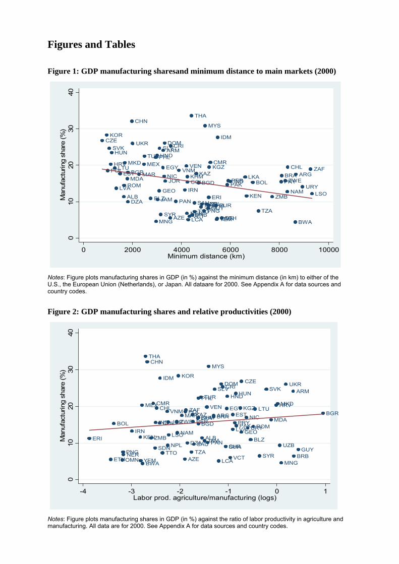
Figures and Tables

Figure 1: GDP manufacturing sharesand minimum distance to main markets (2000)

Notes: Figure plots manufacturing shares in GDP (in %) against the minimum distance (in km) to either of the U.S., the European Union (Netherlands), or Japan. All dataare for 2000. See Appendix A for data sources and country codes.

Figure 2: GDP manufacturing shares and relative productivities (2000)

Notes: Figure plots manufacturing shares in GDP (in %) against the ratio of labor productivity in agriculture and manufacturing. All data are for 2000. See Appendix A for data sources and country codes.

ALB

ARG

ARM

AZE

BGD

BGR

BLZ

BOLBRA

BRB

BWA

CHL

CHN

CMR

COL

CRICZE DOM

DZA

EGY

ERI

EST

ETH

GEO

GHAGUY

HND

HRV

HUN

IDM

IND

IRN

JAM

JOR

KAZ

KEN

KGZ

KHM

KOR

LCA

LKA

LSO

LTU

LVA

MARMDA

MEXMKD

MNG

MYS

NAM

NER

NIC

NPL

OMN

PAK

PAN

PER

PHL

PNG

POL

PRYROM

SAUSDN

SLV

SUR

SVK

SYR

THA

TTO

TUR

TZA

UKR

URY

UZB

VCT

VENVNM

YEM

ZAF

ZMB

ZWE

010

2030

40M

anuf

actu

ring

shar

e (%

)

0 2000 4000 6000 8000 10000Minimum distance (km)

ALB

ARG

ARM

AZE

BGD

BGR

BLZ

BOLBRA

BRB

BWA

CHL

CHN

CMR

COL

CRICZEDOM

DZA

EGY

ERI

EST

ETH

GEO

GHAGUY

HND

HRV

HUN

IDM

IND

IRN

JAM

JOR

KAZ

KEN

KGZ

KHM

KOR

LCA

LKA

LSO

LTU

LVA

MARMDA

MEX MKD

MNG

MYS

NAM

NER

NIC

NPL

OMN

PAK

PAN

PER

PHL

PNG

POL

PRYROM

SAUSDN

SLV

SUR

SVK

SYR

THA

TTO

TUR

TZA

UKR

URY

UZB

VCT

VENVNM

YEM

ZAF

ZMB

ZWE

010

2030

40M

anuf

actu

ring

shar

e (%

)

-4 -3 -2 -1 0 1Labor prod. agriculture/manufacturing (logs)

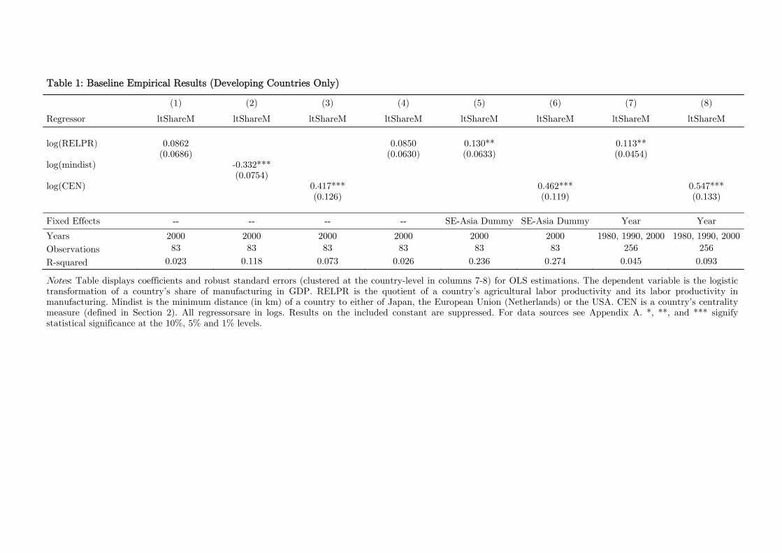
Table 1: Baseline Empirical Results (Developing Countries Only)

(1) (2) (3) (4) (5) (6) (7) (8)

Regressor ltShareM ltShareM ltShareM ltShareM ltShareM ltShareM ltShareM ltShareM

log(RELPR) 0.0862 0.0850 0.130** 0.113** (0.0686) (0.0630) (0.0633) (0.0454) log(mindist) -0.332*** (0.0754) log(CEN) 0.417*** 0.462*** 0.547*** (0.126) (0.119) (0.133)

Fixed Effects -- -- -- -- SE-Asia Dummy SE-Asia Dummy Year Year

Years 2000 2000 2000 2000 2000 2000 1980, 1990, 2000 1980, 1990, 2000 Observations 83 83 83 83 83 83 256 256

R-squared 0.023 0.118 0.073 0.026 0.236 0.274 0.045 0.093

Notes: Table displays coefficients and robust standard errors (clustered at the country-level in columns 7-8) for OLS estimations. The dependent variable is the logistic transformation of a country’s share of manufacturing in GDP. RELPR is the quotient of a country’s agricultural labor productivity and its labor productivity in manufacturing. Mindist is the minimum distance (in km) of a country to either of Japan, the European Union (Netherlands) or the USA. CEN is a country’s centrality measure (defined in Section 2). All regressorsare in logs. Results on the included constant are suppressed. For data sources see Appendix A. *, **, and *** signify statistical significance at the 10%, 5% and 1% levels.

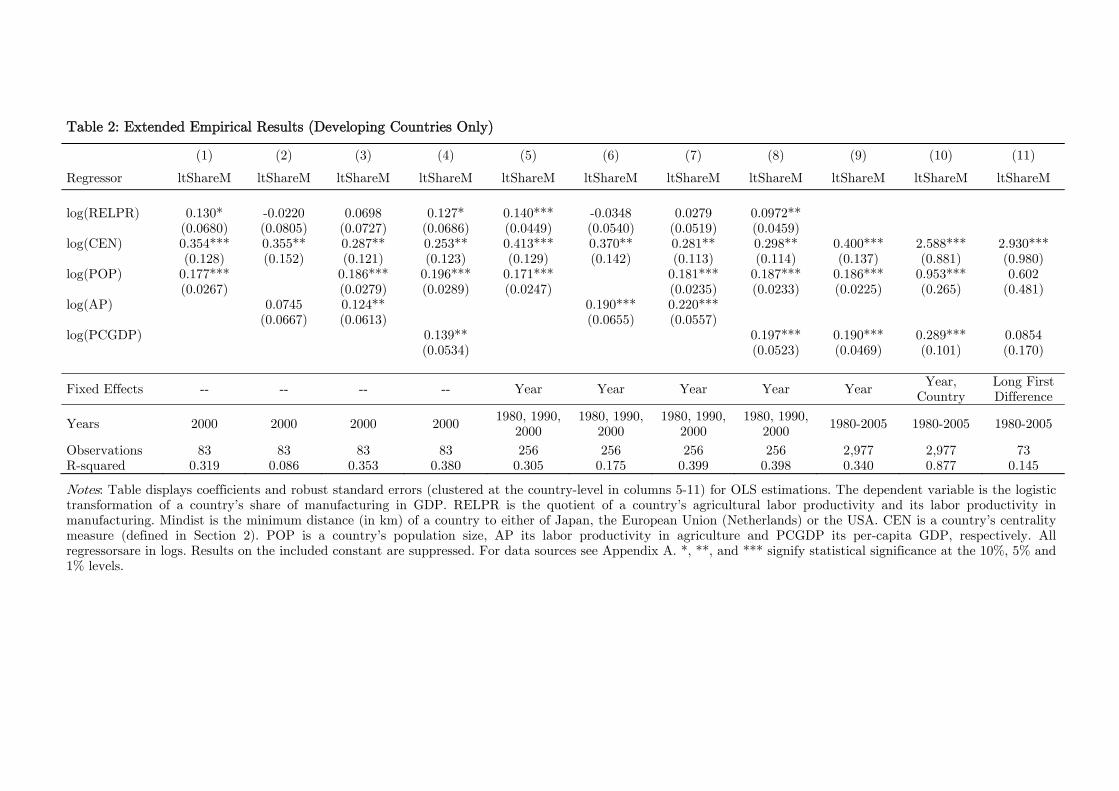
Table 2: Extended Empirical Results (Developing Countries Only)

(1) (2) (3) (4) (5) (6) (7) (8) (9) (10) (11)

Regressor ltShareM ltShareM ltShareM ltShareM ltShareM ltShareM ltShareM ltShareM ltShareM ltShareM ltShareM

log(RELPR) 0.130* -0.0220 0.0698 0.127* 0.140*** -0.0348 0.0279 0.0972** (0.0680) (0.0805) (0.0727) (0.0686) (0.0449) (0.0540) (0.0519) (0.0459) log(CEN) 0.354*** 0.355** 0.287** 0.253** 0.413*** 0.370** 0.281** 0.298** 0.400*** 2.588*** 2.930*** (0.128) (0.152) (0.121) (0.123) (0.129) (0.142) (0.113) (0.114) (0.137) (0.881) (0.980) log(POP) 0.177*** 0.186*** 0.196*** 0.171*** 0.181*** 0.187*** 0.186*** 0.953*** 0.602 (0.0267) (0.0279) (0.0289) (0.0247) (0.0235) (0.0233) (0.0225) (0.265) (0.481) log(AP) 0.0745 0.124** 0.190*** 0.220*** (0.0667) (0.0613) (0.0655) (0.0557) log(PCGDP) 0.139** 0.197*** 0.190*** 0.289*** 0.0854 (0.0534) (0.0523) (0.0469) (0.101) (0.170)

Fixed Effects -- -- -- -- Year Year Year Year Year Year, Country

Long First Difference

Years 2000 2000 2000 2000 1980, 1990,

2000 1980, 1990,

2000 1980, 1990,

2000 1980, 1990,

2000 1980-2005 1980-2005 1980-2005

Observations 83 83 83 83 256 256 256 256 2,977 2,977 73 R-squared 0.319 0.086 0.353 0.380 0.305 0.175 0.399 0.398 0.340 0.877 0.145

Notes: Table displays coefficients and robust standard errors (clustered at the country-level in columns 5-11) for OLS estimations. The dependent variable is the logistic transformation of a country’s share of manufacturing in GDP. RELPR is the quotient of a country’s agricultural labor productivity and its labor productivity in manufacturing. Mindist is the minimum distance (in km) of a country to either of Japan, the European Union (Netherlands) or the USA. CEN is a country’s centrality measure (defined in Section 2). POP is a country’s population size, AP its labor productivity in agriculture and PCGDP its per-capita GDP, respectively. All regressorsare in logs. Results on the included constant are suppressed. For data sources see Appendix A. *, **, and *** signify statistical significance at the 10%, 5% and 1% levels.

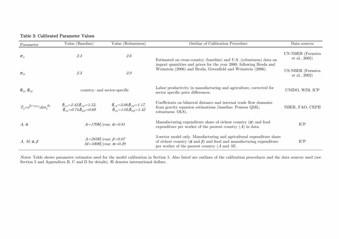
Table 3: Calibrated Parameter Values

Parameter Value (Baseline) Value (Robustness) Outline of Calibration Procedure Data sources

σA 2.3 2.6 Estimated on cross-country (baseline) and U.S. (robustness) data on import quantities and prices for the year 2000, following Broda and Weinstein (2006) and Broda, Greenfield and Weinstein (2006).

UN-NBER (Feenstra et al., 2005)

σM 2.3 2.0 US-NBER (Feenstra et al., 2002)

θAl, θMl country- and sector-specific Labor productivity in manufacturing and agriculture, corrected for sector specific price differences.

UNIDO, WDI, ICP

Tlj=eδ1*d(int)distljδ2 δ1A=2.42,δ1M=1.53,

δ2A=0.74,δ2M=0.69 δ1A=3.08,δ1M=1.17, δ2A=1.05,δ2M=1.42

Coefficients on bilateral distance and internal trade flow dummies from gravity equation estimations (baseline: Poisson QML; robustness: OLS).

NBER, FAO, CEPII

A, α A=170$I/year, α=0.81 Manufacturing expenditure share of richest country (α) and food expenditure per worker of the poorest country (A) in data.

ICP

A, M; α, β A=285$I/year, β=0.07 M=100$I/year, α=0.29

3-sector model only. Manufacturing and agricultural expenditure share of richest country (α and β) and food and manufacturing expenditure per worker of the poorest country (A and M).

ICP

Notes: Table shows parameter estimates used for the model calibration in Section 5. Also listed are outlines of the calibration procedures and the data sources used (see Section 5 and Appendices B, C and D for details). $I denotes international dollars.

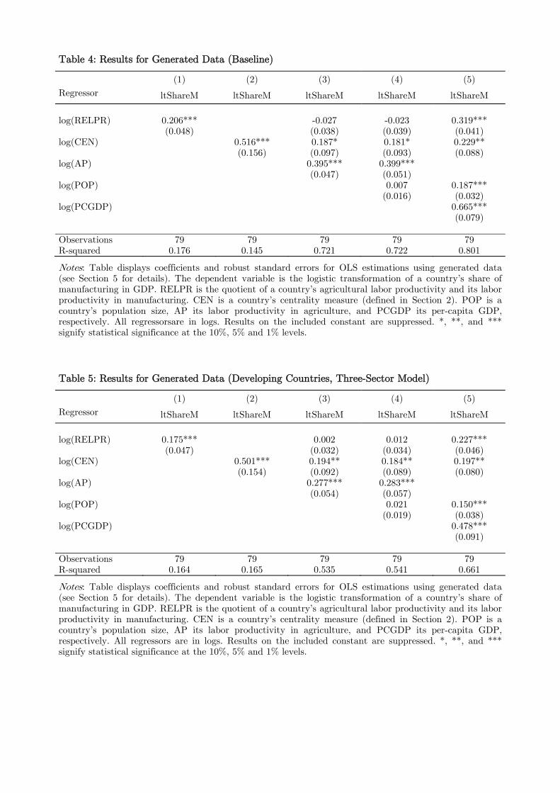
Table 4: Results for Generated Data (Baseline)

(1) (2) (3) (4) (5) Regressor ltShareM ltShareM ltShareM ltShareM ltShareM

log(RELPR) 0.206*** -0.027 -0.023 0.319*** (0.048) (0.038) (0.039) (0.041)log(CEN) 0.516*** 0.187* 0.181* 0.229** (0.156) (0.097) (0.093) (0.088)log(AP) 0.395*** 0.399*** (0.047) (0.051) log(POP) 0.007 0.187*** (0.016) (0.032)log(PCGDP) 0.665*** (0.079) Observations 79 79 79 79 79R-squared 0.176 0.145 0.721 0.722 0.801

Notes: Table displays coefficients and robust standard errors for OLS estimations using generated data (see Section 5 for details). The dependent variable is the logistic transformation of a country’s share of manufacturing in GDP. RELPR is the quotient of a country’s agricultural labor productivity and its labor productivity in manufacturing. CEN is a country’s centrality measure (defined in Section 2). POP is a country’s population size, AP its labor productivity in agriculture, and PCGDP its per-capita GDP, respectively. All regressorsare in logs. Results on the included constant are suppressed. *, **, and *** signify statistical significance at the 10%, 5% and 1% levels.

Table 5: Results for Generated Data (Developing Countries, Three-Sector Model)

(1) (2) (3) (4) (5) Regressor ltShareM ltShareM ltShareM ltShareM ltShareM

log(RELPR) 0.175*** 0.002 0.012 0.227*** (0.047) (0.032) (0.034) (0.046)log(CEN) 0.501*** 0.194** 0.184** 0.197** (0.154) (0.092) (0.089) (0.080)log(AP) 0.277*** 0.283*** (0.054) (0.057) log(POP) 0.021 0.150*** (0.019) (0.038)log(PCGDP) 0.478*** (0.091) Observations 79 79 79 79 79R-squared 0.164 0.165 0.535 0.541 0.661

Notes: Table displays coefficients and robust standard errors for OLS estimations using generated data (see Section 5 for details). The dependent variable is the logistic transformation of a country’s share of manufacturing in GDP. RELPR is the quotient of a country’s agricultural labor productivity and its labor productivity in manufacturing. CEN is a country’s centrality measure (defined in Section 2). POP is a country’s population size, AP its labor productivity in agriculture, and PCGDP its per-capita GDP, respectively. All regressors are in logs. Results on the included constant are suppressed. *, **, and *** signify statistical significance at the 10%, 5% and 1% levels.

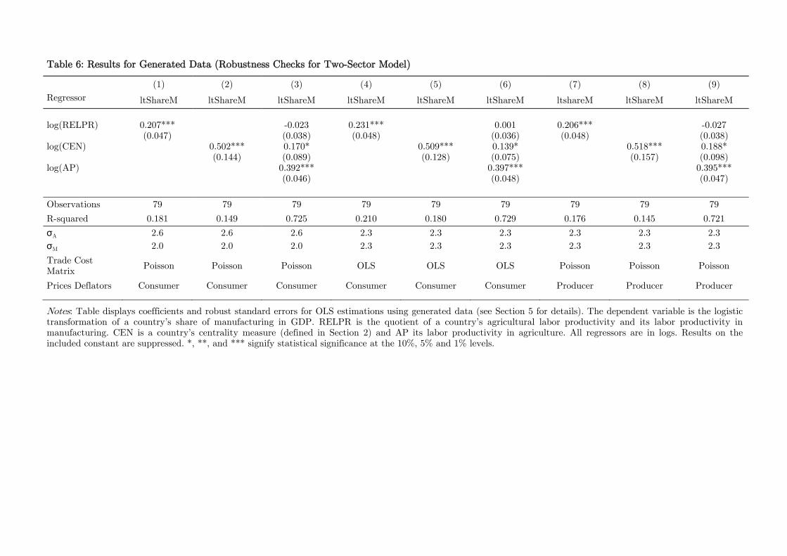
Table 6: Results for Generated Data (Robustness Checks for Two-Sector Model)

(1) (2) (3) (4) (5) (6) (7) (8) (9) Regressor ltShareM ltShareM ltShareM ltShareM ltShareM ltShareM ltshareM ltShareM ltShareM

log(RELPR) 0.207*** -0.023 0.231*** 0.001 0.206*** -0.027 (0.047) (0.038) (0.048) (0.036) (0.048) (0.038) log(CEN) 0.502*** 0.170* 0.509*** 0.139* 0.518*** 0.188* (0.144) (0.089) (0.128) (0.075) (0.157) (0.098) log(AP) 0.392*** 0.397*** 0.395*** (0.046) (0.048) (0.047)

Observations 79 79 79 79 79 79 79 79 79

R-squared 0.181 0.149 0.725 0.210 0.180 0.729 0.176 0.145 0.721

σA 2.6 2.6 2.6 2.3 2.3 2.3 2.3 2.3 2.3 σM 2.0 2.0 2.0 2.3 2.3 2.3 2.3 2.3 2.3

Trade Cost Matrix Poisson Poisson Poisson OLS OLS OLS Poisson Poisson Poisson

Prices Deflators Consumer Consumer Consumer Consumer Consumer Consumer Producer Producer Producer

Notes: Table displays coefficients and robust standard errors for OLS estimations using generated data (see Section 5 for details). The dependent variable is the logistic transformation of a country’s share of manufacturing in GDP. RELPR is the quotient of a country’s agricultural labor productivity and its labor productivity in manufacturing. CEN is a country’s centrality measure (defined in Section 2) and AP its labor productivity in agriculture. All regressors are in logs. Results on the included constant are suppressed. *, **, and *** signify statistical significance at the 10%, 5% and 1% levels.

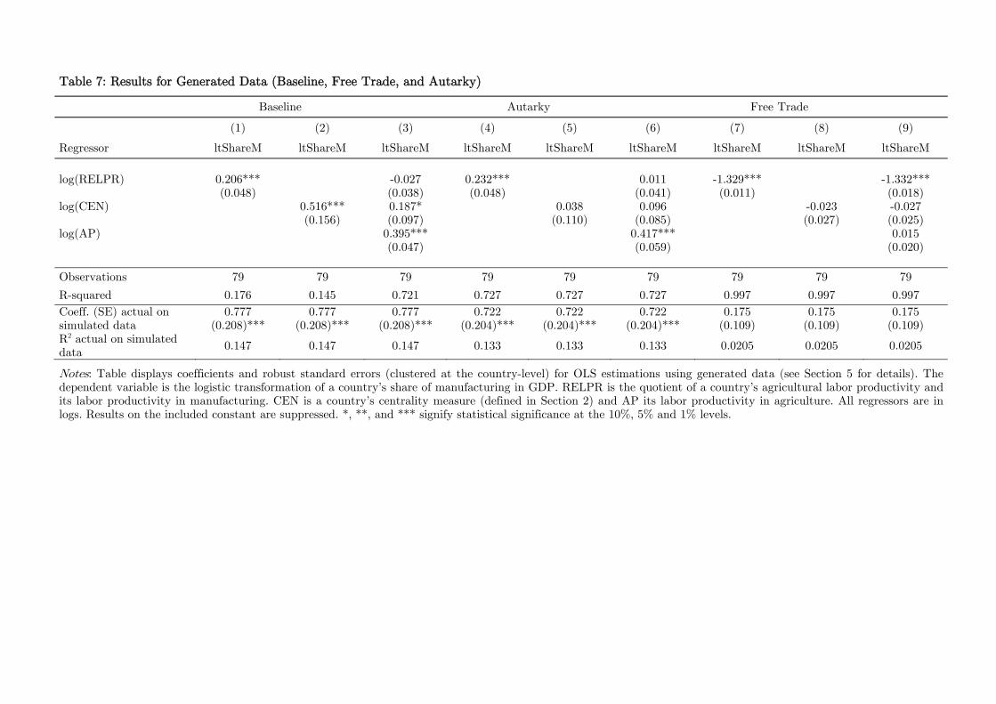
Table 7: Results for Generated Data (Baseline, Free Trade, and Autarky)

Baseline Autarky Free Trade

(1) (2) (3) (4) (5) (6) (7) (8) (9)

Regressor ltShareM ltShareM ltShareM ltShareM ltShareM ltShareM ltShareM ltShareM ltShareM

log(RELPR) 0.206*** -0.027 0.232*** 0.011 -1.329*** -1.332*** (0.048) (0.038) (0.048) (0.041) (0.011) (0.018) log(CEN) 0.516*** 0.187* 0.038 0.096 -0.023 -0.027 (0.156) (0.097) (0.110) (0.085) (0.027) (0.025) log(AP) 0.395*** 0.417*** 0.015 (0.047) (0.059) (0.020) Observations 79 79 79 79 79 79 79 79 79

R-squared 0.176 0.145 0.721 0.727 0.727 0.727 0.997 0.997 0.997 Coeff. (SE) actual on simulated data

0.777 0.777 0.777 0.722 0.722 0.722 0.175 0.175 0.175 (0.208)*** (0.208)*** (0.208)*** (0.204)*** (0.204)*** (0.204)*** (0.109) (0.109) (0.109)

R2 actual on simulated data 0.147 0.147 0.147 0.133 0.133 0.133 0.0205 0.0205 0.0205

Notes: Table displays coefficients and robust standard errors (clustered at the country-level) for OLS estimations using generated data (see Section 5 for details). The dependent variable is the logistic transformation of a country’s share of manufacturing in GDP. RELPR is the quotient of a country’s agricultural labor productivity and its labor productivity in manufacturing. CEN is a country’s centrality measure (defined in Section 2) and AP its labor productivity in agriculture. All regressors are in logs. Results on the included constant are suppressed. *, **, and *** signify statistical significance at the 10%, 5% and 1% levels.

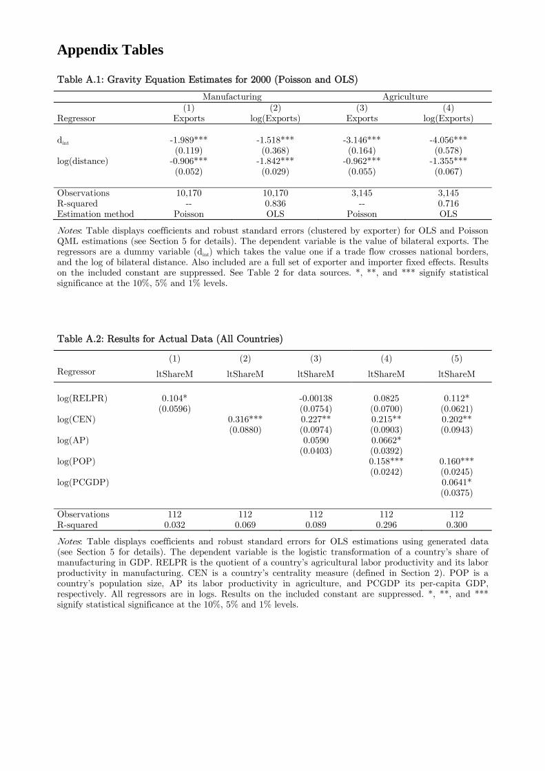
Appendix Tables

Table A.1: Gravity Equation Estimates for 2000 (Poisson and OLS)

Manufacturing Agriculture (1) (2) (3) (4)Regressor Exports log(Exports) Exports log(Exports) dint -1.989*** -1.518*** -3.146*** -4.056*** (0.119) (0.368) (0.164) (0.578)log(distance) -0.906*** -1.842*** -0.962*** -1.355*** (0.052) (0.029) (0.055) (0.067) Observations 10,170 10,170 3,145 3,145R-squared -- 0.836 -- 0.716Estimation method Poisson OLS Poisson OLS

Notes: Table displays coefficients and robust standard errors (clustered by exporter) for OLS and Poisson QML estimations (see Section 5 for details). The dependent variable is the value of bilateral exports. The regressors are a dummy variable (dint) which takes the value one if a trade flow crosses national borders, and the log of bilateral distance. Also included are a full set of exporter and importer fixed effects. Results on the included constant are suppressed. See Table 2 for data sources. *, **, and *** signify statistical significance at the 10%, 5% and 1% levels.

Table A.2: Results for Actual Data (All Countries)

(1) (2) (3) (4) (5) Regressor ltShareM ltShareM ltShareM ltShareM ltShareM

log(RELPR) 0.104* -0.00138 0.0825 0.112* (0.0596) (0.0754) (0.0700) (0.0621)log(CEN) 0.316*** 0.227** 0.215** 0.202** (0.0880) (0.0974) (0.0903) (0.0943)log(AP) 0.0590 0.0662* (0.0403) (0.0392) log(POP) 0.158*** 0.160*** (0.0242) (0.0245)log(PCGDP) 0.0641* (0.0375) Observations 112 112 112 112 112R-squared 0.032 0.069 0.089 0.296 0.300

Notes: Table displays coefficients and robust standard errors for OLS estimations using generated data (see Section 5 for details). The dependent variable is the logistic transformation of a country’s share of manufacturing in GDP. RELPR is the quotient of a country’s agricultural labor productivity and its labor productivity in manufacturing. CEN is a country’s centrality measure (defined in Section 2). POP is a country’s population size, AP its labor productivity in agriculture, and PCGDP its per-capita GDP, respectively. All regressors are in logs. Results on the included constant are suppressed. *, **, and *** signify statistical significance at the 10%, 5% and 1% levels.

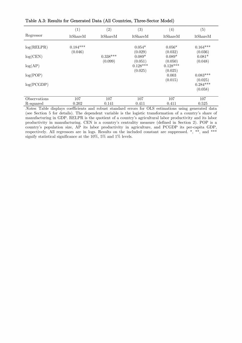
Table A.3: Results for Generated Data (All Countries, Three-Sector Model)

(1) (2) (3) (4) (5) Regressor ltShareM ltShareM ltShareM ltShareM ltShareM

log(RELPR) 0.184*** 0.054* 0.056* 0.164*** (0.046) (0.029) (0.032) (0.036)log(CEN) 0.338*** 0.089* 0.089* 0.081* (0.099) (0.051) (0.050) (0.048)log(AP) 0.128*** 0.128*** (0.025) (0.025) log(POP) 0.003 0.083*** (0.015) (0.025)log(PCGDP) 0.284*** (0.058) Observations 107 107 107 107 107R-squared 0.202 0.141 0.411 0.411 0.525Notes: Table displays coefficients and robust standard errors for OLS estimations using generated data (see Section 5 for details). The dependent variable is the logistic transformation of a country’s share of manufacturing in GDP. RELPR is the quotient of a country’s agricultural labor productivity and its labor productivity in manufacturing. CEN is a country’s centrality measure (defined in Section 2). POP is a country’s population size, AP its labor productivity in agriculture, and PCGDP its per-capita GDP, respectively. All regressors are in logs. Results on the included constant are suppressed. *, **, and *** signify statistical significance at the 10%, 5% and 1% levels.

CENTRE FOR ECONOMIC PERFORMANCE

Recent Discussion Papers

1081 Francesca Cornaglia

Naomi E. Feldman

Productivity, Wages and Marriage: The Case

of Major League Baseball

1080 Nicholas Oulton The Wealth and Poverty of Nations: True

PPPs for 141 Countries

1079 Gary S. Becker

Yona Rubinstein

Fear and the Response to Terrorism: An

Economic Analysis

1078 Camille Landais

Pascal Michaillat

Emmanuel Saez

Optimal Unemployment Insurance over the

Business Cycle

1077 Klaus Adam

Albert Marcet

Juan Pablo Nicolini

Stock Market Volatility and Learning

1076 Zsófia L. Bárány The Minimum Wage and Inequality - The

Effects of Education and Technology

1075 Joanne Lindley

Stephen Machin

Rising Wage Inequality and Postgraduate

Education

1074 Stephen Hansen

Michael McMahon

First Impressions Matter: Signalling as a

Source of Policy Dynamics

1073 Ferdinand Rauch Advertising Expenditure and Consumer

Prices

1072 Alberto Galasso

Mark Schankerman

Carlos J. Serrano

Trading and Enforcing Patent Rights

1071 Daniel Hale

John Coleman

Richard Layard

A Model for the Delivery of Evidence-Based

PSHE (Personal Wellbeing) in Secondary

Schools

1070 David Marsden Individual Voice in Employment

Relationships: A Comparison Under Different

Forms of Workplace Representation

1069 Ross Levine

Alexey Levkov

Yona Rubinstein

Racial Discrimination and Competition

1068 Klaus Adam

Albert Marcet

Internal Rationality, Imperfect Market

Knowledge and Asset Prices

1067 Yanhui Wu A Simple Theory of Managerial Talent, Pay

Contracts and Wage Distribution

1066 Yanhui Wu Managerial Incentives and Compensation in a

Global Market

1065 Nicholas Bloom

Helena Schweiger

John Van Reenen

The Land that Lean Manufacturing Forgot?

Management Practices in Transition

Countries

1064 Klaus Adam

Pei Kuang

Albert Marcet

House Price Booms and the Current Account

1063 Stephen Hansen

Michael McMahon

How Experts Decide: Identifying Preferences

versus Signals from Policy Decisions

1062 Paul Dolan

Daniel Fujiwara

Robert Metcalfe

A Step Towards Valuing Utility the Marginal

and Cardinal Way

1061 Marek Jarocinski

Albert Marcet

Autoregressions in Small Samples, Priors

about Observables and Initial Conditions

1060 Christos Genakos

Kai Uwe Kühn

John Van Reenen

Leveraging Monopoly Power by Degrading

Interoperability: Theory and Evidence from

Computer Markets

1059 Klaus Adam

Albert Marcet

Booms and Busts in Asset Prices

1058 Michael W. L. Elsby

Jennifer C. Smith

Jonathan Wadsworth

The Role of Worker Flows in the Dynamics

and Distribution of UK Unemployment

1057 Fabrice Defever Incomplete Contracts and the Impact of

Globalization on Consumer Welfare

1056 Fadi Hassan The Penn-Belassa-Samuelson Effect in

Developing Countries: Price and Income

Revisited

1055 Albert Marcet

Ramon Marimon

Recursive Contracts

1054 Olivier Cadot

Leonardo Iacovone

Denisse Pierola

Ferdinand Rauch

Success and Failure of African Exporters

1053 Björn Eriksson

Tobias Karlsson

Tim Leunig

Maria Stanfors

Gender, Productivity and the Nature of Work

and Pay: Evidence from the Late Nineteenth-

Century Tobacco Industry

The Centre for Economic Performance Publications Unit

Tel 020 7955 7673 Fax 020 7955 7595

Email info@cep.lse.ac.uk Web site http://cep.lse.ac.uk