ISSN 2042-2695

CEP Discussion Paper No 1206

April 2013

Monopolistic Competition and Optimum

Product Selection: Why and How Heterogeneity Matters

Antonella Nocco

Gianmarco I.P. Ottaviano

Matteo Salto

Abstract After some decades of relative oblivion, the interest in the optimality properties of

monopolistic competition has recently re-emerged due to the availability of an appropriate

and parsimonious framework to deal with firm heterogeneity. Within this framework we

show that non-separable utility, variable demand elasticity and endogenous firm

heterogeneity cause the market equilibrium to err in many ways, concerning the number of

products, the size and the choice of producers, the overall size of the monopolistically

competitive sector. More crucially with respect to the existing literature, we also show that

the extent of the errors depends on the degree of firm heterogeneity. In particular, the

inefficiency of the market equilibrium seems to be largest when selection among

heterogeneous firms is needed most, that is, when there are relatively many firms with low

productivity and relatively few firms with high productivity.

Keywords: monopolistic competition, product diversity, heterogeneity, selection, welfare

JEL Classifications: D4, D6, F1, L0, L1

This paper was produced as part of the Centre’s Globalisation Programme. The Centre for

Economic Performance is financed by the Economic and Social Research Council.

Acknowledgements We thank Olivier Biau, Matthieu Lequien, John Morrow, Peter Neary, Mathieu Parenti,

Jacques Thisse, Evgeny Zhelobodko as well as participants to the conference ‘Industrial

Organization and Spatial Economics’ held in Saint-Petersburg in October 2012, for useful

comments and suggestions. The views expressed here are those of the authors and do not

represent in any manner the EU Commission.

Antonella Nocco is Assistant Professor and Lecturer in Economics, Department of

Management and Economics at Università del Salento. Gianmarco Ottaviano is an Associate of

the Globalisation Programme at the Centre for Economic Performance, London School of

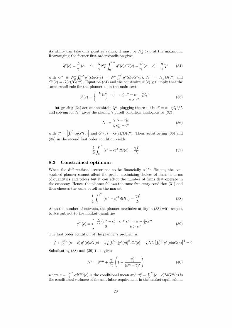
Economics and Political Science. Matteo Salto is an Administrator at the European

Commission.

Published by

Centre for Economic Performance

London School of Economics and Political Science

Houghton Street

London WC2A 2AE

All rights reserved. No part of this publication may be reproduced, stored in a retrieval

system or transmitted in any form or by any means without the prior permission in writing of

the publisher nor be issued to the public or circulated in any form other than that in which it

is published.

Requests for permission to reproduce any article or part of the Working Paper should be sent

to the editor at the above address.

A. Nocco, G. I. P. Ottaviano and M. Salto, submitted 2013

1 Introduction

Do monopolistically competitive industries yield an optimal level of productdiversity? As discussed by Neary (2004), this �classic issue� in industrial or-ganization motivated the canonical formalization of the Chamberlinian model(Chamberlin, 1933) as put forth by Spence (1976) and Dixit and Stiglitz (1977).These propose �reduced form�models that "regard aggregate demands as if theyresult from the maximisation of a utility function de�ned directly over the quan-tities of goods, and the form of the utility function is intended to capture thedesire for variety" (Dixit, 2004, p.125).1 The classic issue can be itself split intofour questions concerning the optimality of the market outcome (Stiglitz, 1975):Are there too few or too many products? Are the quantities of the productstoo small or too large? Are the products supplied by the right set of �rms, orare there �errors�in the choice of technique? Are monopolistically competitiveindustries too large or too small with respect to the rest of the economy?The Chamberlinian model makes four basic assumptions (Bishop, 1967;

Brakman and Heijdra, 2004): the number of sellers in a group of �rms is suf-�ciently large so that each �rm takes the behavior of other �rms in the groupas given; the group is well de�ned and small relative to the economy; productsare physically similar but economically di¤erentiated so that buyers have pref-erences for all types of products (�love for variety�); there is free entry. In thissetup, optimality rests on how the market mechanism deals with the crucialtradeo¤ of �e¢ ciency versus diversity�(Kaldor, 1934).As forcefully highlighted by Dixit and Stiglitz (1975), there are good reasons

to doubt that the market will generally strike the right balance due to the publicnature of diversity in the reduced form approach. As in these models the rangeof products enters utility as a direct argument in addition to the quantitiesconsumed, the range itself becomes a public good whose social bene�t is notfully re�ected in private incentives. In the words of Spence (1976, pp. 230-231):

"[T]here are con�icting forces at work with respect to the numberor variety of products. Because of setup costs, revenues may fail tocover the costs of a socially desirable product. As a result, someproducts may be produced at a loss at an optimum. This is a forcetending towards too few products. On the other hand, there areforces tending towards too many products. First, because �rms holdback output and keep price above marginal cost, they leave moreroom for entry than would marginal cost pricing. Second, whena �rms enter with a new product, it adds its own consumer andproducer surplus to the total surplus, but it also cuts into the pro�tsof the existing �rms. If the cross elasticities of demand are high, thedominant e¤ect may be the second one. In this case entry does notincrease the size of the pie much; it just divides it into more pieces.Thus, in the presence of high cross elasticities of demand, there is atendency toward too many products".

1�Structural�models, instead, "give an explicit model of a consumer�s choice where diver-sity plays a role; discrete choice from a collection of products di¤erentiated by location in acharacteristic space in the most common framework" (Dixit, 2004, p.125). See Anderson, dePalma and Thisse (1992) for microfoundations of the representative-consumer reduced formapproach based on random-utility models of discrete choice.

2

As the issue of optimal product diversity does not admit a general settlement,explicit models with a detailed formulation of demand are used to isolate andanalyze the four questions described above. The canonical choice is to model aneconomy consisting of two sectors. The �rst sector is monopolistically competi-tive and is the focus of the analysis. The second sector is perfectly competitiveand represents the rest of the economy. Its purpose is to hold factor prices incheck and to create the slack needed to answer the question whether the mo-nopolistically competitive sector is too small or too big. This way the market isallowed to eventually misallocate resources not only within the monopolisticallycompetitive sector but also between this sector and the rest of the economy.The best known insights of the canonical model concern the special case in

which the �group utility�de�ned over di¤erentiated products is separable acrossthem, the demand of each product is CES and �rms are homogeneous. In thiscase, the model shows that the �rst-best (�unconstrained�) optimum calls forlarger �rms and more product variety than the market provides. From a nor-mative perspective, however, this result is traditionally regarded of little prac-tical relevance for policy intervention because implementing the unconstrainedoptimum requires the use of lump-sum instruments that are hardly available inreality. These are needed to subsidize the entry of �rms that otherwise wouldnot cover their setup (�entry�) costs due to marginal cost pricing at the optimum.A lot of attention has, therefore, been devoted to the �constrained�optimum inwhich the monopolistically competitive sector is �nancially self-su¢ cient. Underthis constraint, the market is shown to provide the optimal number of products,the optimal size �rms and hence the optimal size of the sector.The robustness of these results has been investigated along several dimen-

sions, with particular attention devoted to the impact of variable demand elas-ticity and �rm heterogeneity. These extensions are already discussed by Stiglitz(1975), Spence (1976) and Dixit and Stiglitz (1977), who show that, when theelasticity of demand is allowed to vary, the market equilibrium ceases to beconstrained optimal. In particular, products are too many (too few) and aresupplied in too small (too large) quantities when the elasticity of �product utility�is increasing (decreasing) in the quantity consumed. As for �rm heterogeneity,Dixit and Stiglitz (1977) consider a variant of their model in which there are twogroups of di¤erentiated products that are perfect substitutes for each other witheach group having CES sub-utility. Both �xed and marginal costs are allowed todi¤er between the two groups but not within them. Dixit and Stiglitz (1977) usethis variant to show that the determination of the set of products to be supplieddepends on a richer list of factors: �xed and marginal costs, the elasticity of thedemand schedule, the level of the demand schedule and the cross-elasticities ofdemand. As a result, constrained optimality eventually applies only to a zero-measure set of parametrizations. A more exhaustive treatment of this issue canbe found in Spence (1976) while Stiglitz (1975) reaches similar conclusions ina model of the capital market in which �rms with heterogeneous costs issuesecurities whose returns are imperfectly correlated with each other.After some decades of relative oblivion, interest in the optimality properties

of monopolistic competition has recently re-emerged due to the �heterogeneous�rms revolution�in international trade theory (Melitz and Redding, 2012). Thishas been initiated by Melitz (2003), who shows that a Dixit-Stiglitz model withCES demand, endogenous �rm heterogeneity and �xed export costs (but withoutthe homogeneous good sector) predicts �new� gains from trade liberalization

3

through the selection of the most e¢ cient �rms. Subsequent papers show thata similar result holds when demand exhibits variable elasticity, though �xedexport costs are not necessarily needed for the result to materialize in this case(Melitz and Ottaviano, 2008; Behrens and Murata, 2012).2

The validity of these (among other) insights on international trade issueswhen alternative speci�cations of demands are allowed for is discussed by Zh-elobodko, Kokovin, Parenti, and Thisse (2012). Using a framework with variableelasticity of substitution (VES), they show that CES is just a knife-edge case.While this �nding is reminiscent of the conclusions by Stiglitz (1975), Spence(1976) and Dixit and Stiglitz (1977), Zhelobodko, Kokovin, Parenti, and Thisse(2012) do not discuss its implications for optimum product variety as those earlycontributors do. This is done, instead, by Dhingra and Morrow (2012) who fullycharacterize the optimality properties of a general demand system derived fromseparable �group utility�. Their normative analysis thus complements the posi-tive analysis of Zhelobodko, Kokovin, Parenti, and Thisse (2012), showing that,in the absence of the homogeneous sector, the market outcome achieves the (un-constrained) optimum under CES but not under VES. When a homogeneoussector is instead introduced, Melitz and Redding (2012) show that CES leadsto constrained rather than unconstrained optimality due to the misallocation ofresources between sectors. In other words, with CES �rm heterogeneity doesnot change the welfare insights of the original Dixit-Stiglitz framework whilethings change in the case of VES.The present paper goes back to the full set of classic questions laid down

at the beginning of this introduction, with renewed emphasis on the questionwhether in the market equilibrium the products are supplied by the right setof �rms. It does so in a Melitzian framework of endogenous �rm heterogeneitywith variable demand elasticity. Its aim is twofold. It shows that, with variabledemand elasticity and endogenous �rm heterogeneity, the market outcome errswith respect to the number of products, the size and the choice of producers,and the overall size of the monopolistically competitive sector. More cruciallywith respect to the existing literature, it also shows that the extent of the errorsdepends on the degree of �rm heterogeneity.None of the papers previously cited simultaneously addresses the four classic

questions on the optimality of monopolistic competition in a framework withvariable demand elasticity and endogenous �rm heterogeneity. Moreover, noneof them provides a systematic quantitative analysis of the impact of di¤erentdegrees of �rm heterogeneity on the extent of market ine¢ ciencies. The dis-cussion in Spence (1976) is systematic but qualitative, while Dixit and Stiglitz(1977) con�ne themselves to the special scenario discussed above. Dhingra andMorrow (2012) are closer to what the present paper tries to achieve but thefocus of their comparative statics is on the parametrization of demand ratherthan on the parametrization of �rm heterogeneity. In addition, not having thehomogeneous good sector prevents them from discussing between-sector mis-allocation. Di¤erently, Stiglitz (1975) presents comparative statics results onthe heterogeneity parameters but his heterogeneity is not endogenous and hisapproach, based on a utility de�ned over alternative portfolios of assets, is quitedistinct from the canonical model of monopolistic competition.

2See Arkolakis, Costinot and Rodriguez-Clare (2010) as well as Melitz and Redding (2013)for a discussion of the actual novelty of these �ndings.

4

Clearly, as pointed out by Stiglitz (1975) and others, without some appropri-ate parametrization of the problem, it would be hard to cut any new ground onthe issues of interest. We rely on the speci�c parametrization of linear demandintroduced by Ottaviano, Tabuchi and Thisse (2002) as applied to endogenous�rm heterogeneity by Melitz and Ottaviano (2008). This parametrization is lessgeneral than the VES systems studied by Dhingra and Morrow (2012) and Zh-elobodko, Kokovin, Parenti, and J. F. Thisse (2012) in terms of product utilitybut allows for cross-product e¤ects that are absent in the former paper andonly touched upon in the latter. For ease of exposition, in the main text we alsofocus on a speci�c but commonly used Pareto parametrization of �rm hetero-geneity, relegating the discussion of the validity of some key results in the caseof a generic continuous parametrization to the appendix. There we also presentthe welfare analysis of the degenerate case in which �rms are homogeneous asdiscussed by Ottaviano and Thisse (1999) for the same demand system.The rest of the paper is organized in six sections. Section 2 brie�y presents

the model by Melitz and Ottaviano (2008). Sections 3 and 4 respectively deriveand compare the market equilibrium and the (unconstrained) optimum. Section5 investigates the impact of �rm heterogeneity on the gap between the equilib-rium and optimum outcomes. Section 6 discusses the constrained optimum.Section 7 concludes.

2 The model

Following Melitz and Ottaviano (2008), consider an economy populated by Lconsumers, each endowed with one unit of labor. Preferences are de�ned overa continuum of di¤erentiated varieties indexed i 2 , and a homogeneous goodindexed 0. All consumers own the same initial endowment q0 of this good andshare the same utility function given by

U = qc0 + �

Zi2

qci di�1

2

Zi2

(qci )2di� 1

2�

�Zi2

qci di

�2(1)

with positive demand parameters �, � and , the latter measuring the �love forvariety�and the others measuring the preference for the di¤erentiated varietieswith respect to the homogeneous good. The initial endowment q0 of the homo-geneous good is assumed to be large enough for its consumption to be strictlypositive at the market equilibrium and optimal solutions.Labor is the only factor of production. It can be employed for the production

of the homogeneous good under perfect competition and constant returns toscale with unit labor requirement equal to one. It can also be employed for theproduction of the di¤erentiated varieties under monopolistic competition. Thetechnology requires a preliminary R&D e¤ort of f > 0 units of labor to design anew variety and its production process, which is also characterized by constantreturns to scale. The R&D e¤ort leads to the design of a new variety withcertainty whereas the unit labor requirement c of the corresponding productionprocess is uncertain, being randomly drawn from a continuous distribution withcumulative density

G(c) =

�c

cM

�k, c 2 [0; cM ] (2)

5

This corresponds to the empirically relevant case in which marginal produc-tivity 1=c is Pareto distributed with shape parameter k � 1 over the support[1=cM ;1). Hence, as k rises, density is skewed towards the upper bound of thesupport of G(c).3 The R&D e¤ort cannot be recovered and this gives rise to asunk setup (�entry�) cost.

3 Equilibrium and optimum

3.1 The market outcome

In the decentralized equilibrium consumers maximize utility under their budgetconstraints, �rms maximize pro�ts given their technological constraints, andmarkets clear. It is assumed that the labor market as well as the market of thehomogeneous good are perfectly competitive. This good is chosen as numeraire,which then implies that the wage equals one. The market of di¤erentiatedvarieties is, instead, monopolistically competitive with a one-to-one relationbetween �rms and varieties.The �rst order conditions for utility maximization give individual inverse

demand for variety i aspi = �� qci � �Qc (3)

whenever qci > 0, with Qc =

Ri2 q

ci di. Demand for consumed varieties can be

derived from (3) as

qi � Lqci =�L

�N + � L pi +

�N

�N +

L

�p; 8i 2 � (4)

where the set � is the largest subset of such that demand is positive, Nis the measure (�number�) of varieties in � and �p = (1=N)

Ri2� pidi is their

average price. Variety i belongs to this set when

pi �1

�N + ( �+ �N �p) � pmax (5)

where pmax � � represents the price at which demand for a variety is driven tozero.4

When a variety is produced by a �rm with unit labor requirement c, thecorresponding �rst order conditions for pro�t maximization are satis�ed by anoutput level equal to

qm(c) =

�L2 (c

m � c) if c � cm = pmax = �� �LQ

m

0 if c > cm(6)

where �m�labels equilibrium variables and Qm =R cm0qm(c)dG(c) is the total

supply of di¤erentiated varieties. Expression (6) de�nes a cuto¤rule for survival:3While the analysis in the main text rests on the Pareto distribution, several results have

more general validity as discussed in Appendix A.4Melitz and Ottaviano (2008) show that rewriting the indirect utility function in terms of

average price and price variance reveals that it decreases with average prices �p, but rises withthe variance of prices �2p (holding �p constant), as consumers then re-optimize their purchasesby shifting expenditures towards lower priced varieties as well as the numeraire good. Notealso that the demand system exhibits �love of variety�: holding the distribution of pricesconstant (namely holding the mean �p and variance �2p of prices constant), utility rises withproduct variety N .

6

only entrants that are productive enough (c � cm) eventually produce. For themthe price that corresponds to the pro�t-maximizing output qm(c) is pm(c) =(cm + c) =2, implying markup �m(c) = pm(c)� c = (cm � c) =2 and maximizedpro�t

�(c) =L

4 (cm � c)2 (7)

Due to free entry and exit, in equilibrium expected pro�t is exactly o¤set bythe sunk entry cost Z cm

0

�(c)dG(c) = f

Given (2) and (7), this �free entry condition�can be rewritten as�cm

cM

�kL (cm)

2

2 (k + 1)(k + 2)= f (8)

where, due to the law of large numbers, G(cm) = (cm=cM )k is the ex ante

probability that an entrant will produce as well as the ex post share of entrantsthat eventually produce while L (cm)2 =[2 (k+1)(k+2)] is the ex ante expectedpro�t conditional on producing as well as the ex post average pro�t of producers.Condition (8) can be solved for the unique equilibrium cuto¤ marginal cost

cm =

"2 (k + 1)(k + 2) (cM )

kf

L

# 1k+2

(9)

Finally, the number of producers can be determined as a function of cm byobserving that marginal �rms with unit labor requirement c = cm make zeropro�t, i.e. p(cm) = cm = pmax. Recalling (5), that implies the following �zerocuto¤ pro�t condition�

cm =1

�Nm + ( �+ �Nm�pm) (10)

where, again due to the law of large numbers, �pm is the ex ante expected priceconditional on producing as well as the ex post average price of producers: �pm =R cm0p(c)dGm(c) with Gm(c) = G(c)=G(cm) = (c=cm)k. The �zero cuto¤ pro�t

condition�can then be solved to obtain the equilibrium number of producers(and varieties) as a function of the equilibrium cuto¤ as

Nm =2 (k + 1)

�

�� cmcm

(11)

with the corresponding equilibrium number of entrants given byNmE = Nm=G(cm) =

Nm (cM=cm)

k.

3.2 The optimal outcome

As the quasi-linearity of (1) implies transferable utility, social welfare may beexpressed as the sum of all consumers�utilities. This implies that the �rst best(�unconstrained�) planner chooses the number of varieties and their output lev-els so as to maximize the social welfare function given by individual utility (1)

7

times the number of consumers L, subject to the resource constraint, the vari-eties�production functions and the stochastic �innovation production function�(i.e. the mechanism that determines each variety�s unit labor requirement as arandom draw from G(c) after f units of labor have been allocated to R&D).Speci�cally, given (1), the planner chooses the number NE of R&D projects

and the output levels of associated varieties so as to maximize social welfare

W = qc0L+ �NER cM0

[qc(c)L] dG(c)� 12 LNE

R cM0

[qc(c)L]2dG(c)

� 12�L

�NE

R cM0

[qc(c)L] dG(c)�2 (12)

with respect to qc0, qc(c) and NE subject to the aggregate resource constraint

qc0L+ fNE +NE

Z cM

0

cqc(c)LdG(c) = L+ q0L (13)

stating that the supply of the homogeneous good (qc0L), the supply of di¤er-entiated varieties (NE

R cM0

cqc(c)LdG(c)) and the R&D investment (fNE) arecostrained by the amount of available resources (L+ q0L).After substituting (13) into (12), the planner�s problem can be rewritten as

the maximization of

W = L+ q0L� fNE +NER cM0

(�� c) q(c)dG(c)� 12 LNE

R cM0

[q(c)]2dG(c)� 1

2�L

�NE

R cM0

q(c)dG(c)�2 (14)

with respect to q(c) and NE . The corresponding �rst order conditions are then:

@W@q(c) =

hNE (�� c)�

LNEq(c)��L (NE)

2 R cM0

q(c)dG(c)idG(c) = 0 8c

(15)@W@NE

= �f +R cM0

(�� c) q(c)dG(c)� 12 L

R cM0

[q(c)]2dG(c)

� �LNE

�R cM0

q(c)dG(c)�2= 0

(16)

Rearranging (15) shows that optimal output qo(c) has to satisfy

q(c) =L

(�� c)� �

NE

Z cM

0

q(c)dG(c) =L

(�� c)� �

Q

with Q � LRi2 q

ci di = NE

R cM0

q(c)dG(c), i.e.

qo(c) =

�L (c

o � c) if c � co = �� �LQ

o

0 if c > co(17)

where �o� labels �rst best optimum variables and Qo = NoE

R cM0

qo(c)dG(c) isthe optimum total supply of di¤erentiated varieties. Result (17) reveals that,just like the market, also the planner follows a cuto¤ rule allowing only for theproduction of varieties whose unit labor requirements are low enough: qo(c) �0 only for c � co. We can thus de�ne the conditional distribution of unitinput requirements for varieties that the planner actually produces as Go(c) =G(c)=G(co). The number No of those varieties thus satis�es No = G(co)No

E .Expressions (17) and (3) can be used to show that the �rst best output

levels would clear the market in the decentralized scenario only if each producerpriced at its own marginal cost. To see this, note that (3) implies q(c) =

8

[� � p(c)]L= � �Q= . Then, imposing q(c) = qo(c) = (co � c)L= and Q =Qo = (�� co)L=� from (17) respectively on the left and on the right hand sidesof q(c) = [�� p(c)]L= � �Q= gives p(c) = c.Integrating (15) gives

Qo = No

+ �No

L

(�� �co)

where �co =R co0cdGo(c). Substituting this result in co = � � �Qo=L from (17)

and solving for No gives a planner�s cuto¤ condition analogous to the market�zero cuto¤ pro�t condition�(10)

No = NoEG(c

o) = (k + 1)

�

�� coco

(18)

In order to �nd a second condition analogous to the market �free entry con-dition� (8), we can substitute the optimal quantities from (17) as well as theoptimal number of varieties (18) in the second condition in (16) to obtain�

co

cM

�kL (co)

2

(k + 1)(k + 2)= f (19)

so that the �rst best cuto¤ marginal cost evaluates to

co =

" (k + 1)(k + 2) (cM )

kf

L

# 1k+2

(20)

This then determines the �rst best number of varieties through (18). To sumup, (20) and (18) are the �rst best planner�s analogues of expressions (9) and(11) derived for the market equilibrium.

4 Equilibrium vs. optimum

There are two dimensions along which the e¢ ciency of the market outcome canbe evaluated: the number of varieties actually produced Nm and the (condi-tional) cost distribution of the �rms producing them as dictated by the cuto¤cm. In turn, the cost distribution determines the e¢ ciency of the correspondingdistributions of �rm sizes and prices.5

The tradeo¤s the �rst best planner faces when �rms are heterogeneous canbe highlighted by rewriting the �rst best objective (12) in terms of means andvariances of the distribution G(c) as follows

W =�L+ q0L+NE

��bq � 1

2 Lbq2 � 1

2�LNEbq2 � bcbq � f��� hNE � 12 Lb�2q + b�cq�i

(21)where bc = R cM

0cdG(c) is the unconditional mean unit labor requirement, bq =R cM

0q(c)dG(c) and b�2q = nR cM0 [q(c)]

2dG(c)� bq2o are the unconditional mean

5Dhingra and Morrow (2012) provide a detailed discussion of these issues that emphasizesthe role of alternative parametrizations of demand when utility is separable. The bias inmarket allocations by demand characteristics is summarized in their Table 2. If we alsoassumed separability (by imposing � = 0), our demand system would be compatible with theparametrizations classi�ed in the upper right hand corner of that table.

9

and variance of quantities, and b�cq = �R cM0 cq(c)dG(c)� bcbq is the convariancebetween quantities and unit input requirements.6 The �rst bracketed term onthe right hand side of (21) corresponds to the planner�s objective when marginalcosts are homogeneous. Here the tradeo¤s are in terms of: (a) average quantityvs. average marginal cost; (b) number of varieties vs. �xed costs. The secondbracketed term has to be considered when unit labor requirements are hetero-geneous. It shows that, due to love of variety, consumers dislike a consumptionbundle in which the quantity consumed varies across varieties. Formally, theydislike a consumption bundle with large deviations from the average (large b�q),the more so the stronger the love of variety (larger ). On the other hand, thereis a penalty in o¤ering a basket of varieties with small deviations around theaverage as higher productivity could be achieved by assigning little productionto varieties with high marginal costs (b�cq < 0).4.1 Selection

Comparing the equilibrium cuto¤with the optimal one is straightforward. Specif-ically, comparing expressions (9) with (20) reveals that cm = 21=(k+2)co, whichimplies co < cm. Accordingly, varieties with c 2 [co; cm] should not be supplied.We thus have:

Proposition 1 (Selection) Firm selection in the market equilibrium is weakerthan optimal.

The intuition behind this proposition can be gauged by recalling that, asdiscussed in Section 3.1, in the market equilibrium the markup of a �rm withmarginal cost c equals �m(c) = pm(c)� c = (cm � c) =2. Accordingly, consump-tion is ine¢ ciently biased against the di¤erentiated varieties and in favor of thenumeraire good as the prices of the former are ine¢ ciently high.Di¤erences in the strength of selection map into aggregate performance.

In particular, de�ning aggregate productivity �� as average output per workerweighted by �rm size, expressions (2), (6) and (17) imply

��j �R cj0q(c)dG(c)R cj

0cq(c)dG(c)

=k + 2

k

1

cj

with j 2 fm; og Hence, the cuto¤ ranking co < cm maps into the productivityranking ��o > ��m, with ��o = 21=(k+2) ��m, giving rise to the following result:

Corollary 2 (Average productivity) Aggregate productivity in the marketequilibrium is lower than optimal.

4.2 Firm size

Proposition 1 has also implications in terms of optimality of the �rm size dis-tribution. To see this, one can use (6) and (17) to rewrite output levels as

qm(c) =L

2 (cm � c) and qo(c) =

L

(co � c)

6With homogeneous unit labor requirements we would have b�q = b�cq = 0 and the planner�sobjective boils down to the one in Ottaviano and Thisse (1999). See Appendix B for furtherdetails.

10

Since cm = 21=(k+2)co implies co < cm, it is readily seen that qm(c) > qo(c)if and only if c >

�2� 21=(k+2)

�co, which falls in the relevant interval [0; co]

given that 0 <�2� 3

p2�<�2� 21=(k+2)

�< 1. Hence, with respect to the

optimum, the market equilibrium undersupplies varieties with marginal costc 2 [0;

�2� 21=(k+2)

�co) and oversupplies varieties with marginal cost c 2

(�2� 21=(k+2)

�co; cm]. Hence, we have:

Corollary 3 (Within-sector misallocation) The market equilibrium over-supplies high cost varieties and undersupplies low cost ones with respect to theoptimum.

In other words, misallocation materializes as a lack of market concentration:in the market equilibrium there are relatively too many small �rms and relativelytoo few large �rms with respect to the optimum. The intuition behind thiscorollary can be explained as follows. The markup �m(c) = (cm � c) =2 is adecreasing function of c. This implies that more productive �rms do not passon their entire cost advantage to consumers as they absorb part of it in themarkup. As a result, the price ratio of less to more productive �rms is smallerthan their cost ratio and thus the quantities sold by less productive �rms are toolarge from an e¢ ciency point of view relative to those sold by more productive�rms.Turning to average �rm size q, given (2), expressions (6) and (17) together

with expressions (9) and (20) imply

qm =

Z cm

0

qm(c)dGm(c) =L

2

1

k + 1cm (22)

qo =

Z co

0

qo(c)dGo(c) =L

1

k + 1co = 2

k+1k+2 qm

so that the cuto¤ ranking co < cm dictates the average output ranking qm < qo.Accordingly, we can write:

Corollary 4 (Average �rm size) In the market equilibrium �rms are onaverage smaller than optimal.

The intuition behind this corollary follows from the discussion of the previousone: a lower cuto¤ with markup pricing makes �rms on average larger in theoptimum than in the market equilibrium.Finally, given (11), (18) and (22), the total output of the di¤erentiated

varieties evaluates to Nmqm = (L=�) (�� cm) and Noqo = (L=�) (�� co) atthe market equilibrium and at the optimum respectively. Hence, co < cm impliesNoqo > Nmqm and we have:

Corollary 5 (Between-sector misallocation) In the market equilibrium thetotal supply of di¤erentiated varieties is smaller than optimal.

4.3 Product variety and entry

The equilibrium is suboptimal also when it comes to the number of varietiessupplied. However, given (11) and (18), the ranking of cuto¤s co < cm does not

11

allow to rank Nm and No unambiguously. In particular, since cm = 21=(k+2)co,we have Nm > No as long as

� > �1 �co

2k+1k+2 � 1

=1

2k+1k+2 � 1

" (k + 1)(k + 2) (cM )

kf

L

# 1k+2

(23)

which is the case when � as well as L are large and when , f as well as cM aresmall. Hence, we can state the following result:

Corollary 6 (Product variety) Product variety is richer (poorer) in the mar-ket equilibrium than in the optimum when varieties are close (far) substitutes,the sunk entry cost is small (large), market size is large (small) and the di¤er-ence between the highest and the lowest possible cost draws is small (large).

This corollary has an interesting implication for the impact of larger mar-ket size, driven for example by the integration of previously autarkic nationalmarkets. In this scenario, it could well be that each national market on its ownis small enough to entail � < �1 whereas the internationally integrated marketis large enough to entail � > �1. Then, according to the corollary, market in-tegration would cause the transition from a situation in which product varietyis ine¢ ciently poor (Nm < No) to a situation in which it becomes ine¢ cientlyrich (Nm > No).Turning to entry, the equilibrium number of entrants is given by

N jE =

N j

G(cj)= N j

�cMcj

�k(24)

with j 2 fm; og. Then, together with (11) and (18) as well as (9) and (20),expression (24) can be used to show that cm = 21=(k+2)co imply Nm

E > NoE as

long as

� > �2 �22=(k+2) � 121=(k+2) � 1c

o =22=(k+2) � 121=(k+2) � 1

" (k + 1)(k + 2) (cM )

kf

L

# 1k+2

(25)

which is the case when � as well as L are large and , f as well as cM are small.This leads to:

Corollary 7 (Entry) More (fewer) �rms enter in the market equilibrium thanin the optimum if varieties are close (far) substitutes, the sunk entry cost issmall (large), market size is large (small) and the di¤erence between the highestand the lowest possible cost draws is small (large).

As larger market size reduces �2, it causes the transition from a situationin which the resources devoted to develop new varieties are ine¢ ciently small(Nm

E < NoE) to a situation in which they are ine¢ ciently large (N

mE > No

E).Given that (23) and (25) imply �1 < �2, corollaries 6 and 7 together imply

that the market provides too little entry with too little variety for � < �1 andtoo much entry with too much variety for � > �2. For �1 < � < �2 it provides,instead, too much variety and too little entry.

12

5 The impact of �rm heterogeneity

We now turn to the relation between the degree of heterogeneity and the ex-tent of the market ine¢ ciency. The key question here is whether or not theine¢ ciency of the market equilibrium is largest when selection is needed most,that is, when there are a lot of low productivity �rms and few high productivityones.As discussed by Ottaviano (2012), the scale and shape parameters of the

Pareto distribution (2) regulate the �heterogeneity�of cost draws along two di-mensions: �richness�and �evenness�(Maignan, Ottaviano, Pinelli and Rullani,2003). First, the scale parameter cM quanti�es �richness�, de�ned as the mea-sure (�number�) of di¤erent unit labor requirements that can be drawn. LargercM leads to a rise in heterogeneity along the richness dimension, and this isachieved by making it possible to draw also larger unit labor requirements thanthe original ones. Second, the shape parameter k is an inverse measure of �even-ness�, de�ned as the similarity between the probabilities of those di¤erent drawsto happen. When k = 1, the unit labor requirement distribution is uniformon [0; cM ] with maximum evenness. As k increases, the unit labor requirementdistribution becomes more concentrated at higher unit labor requirements closeto cM : evenness falls. As k goes to in�nity, the distribution becomes degener-ate at cM : all draws deliver a unit labor requirement cM with probability one.Hence, smaller k leads to a rise in heterogeneity along the evenness dimension,and this is achieved by making low unit labor requirements more likely with-out changing the unit labor requirements that are possible. Accordingly, morerichness (larger cM ) comes with higher average unit labor requirement (�cost-increasing richness�), more evenness (smaller k) comes with lower average unitlabor requirement (�cost-decreasing evenness�).Given the cuto¤ expressions (9) and (20), more heterogeneity has di¤erent

impacts on selection depending on whether it comes through more richness orevenness. To see this, rewrite (9) and (20) as:�

cm

cM

�k "L

4

2 (cm)2

(k + 2) (k + 1)

#= f

�co

cM

�k "L

2

2 (cm)2

(k + 2) (k + 1)

#= f

where (cm=cM )k and (co=cM )

k are the shares of viable varieties and the brack-eted terms are average �rm pro�t for the market equilibrium and average sur-plus per variety for the optimum respectively. For any given cuto¤s, morecost-increasing richness (larger cM ) decreases the left hand sides of both expres-sions through its depressing e¤ect on the share of viable varieties. As the righthand sides are constant, (9) and (20) can keep on holding only if the cuto¤srise. Di¤erently, for any given cuto¤s (smaller than cM ), more cost-decreasingevenness (smaller k) increases the left hand sides of both expressions throughits enhancing e¤ect on both the share of viable varieties and average pro�t orsurplus. Again, as the right hand sides are constant, (9) and (20) can keep onholding only if the cuto¤s fall. Hence, while more cost-increasing richness makesselection softer, more cost-decreasing evenness makes it tougher.When we focus on the percentage deviation of the market equilibrium from

13

the optimum, only the change in evenness matters for several outcomes. Specif-ically, given cm = 21=(k+2)co, more eveness (smaller k) leads to a larger per-centage gap in the cuto¤s between the market equilibrium and the optimum((cm � co) =co rises) whereas more richness is immaterial. Hence, we have:

Proposition 8 (Heterogeneity and selection) More cost-decreasing even-ness increases the percentage gap in the cuto¤s between the market equilibriumand the optimum. Cost-increasing richness has no impact on this gap.

As in the case of Proposition 1, Proposition 8 gives rise to a series of parallelcorollaries. First, given ��o = 21=(k+2) ��m, smaller k increases the percentageaggregate productivity gap between the market equilibrium and the optimum(���o � ��m

�=��o rises). We can therefore state:

Corollary 9 (Heterogeneity and productivity) More cost-decreasing even-ness increases the percentage gap in the aggregate productivity between the mar-ket equilibrium and the optimum. Cost-increasing richness has no impact onthis gap.

Second, recall that, with respect to the optimum, the market equilibriumundersupplies varieties with marginal cost c 2 [0;

�2� 21=(k+2)

�co) and over-

supplies varieties with marginal cost c 2 (�2� 21=(k+2)

�co; cm]. When k falls�

2� 21=(k+2)�co=cm also falls whereas it does not change when cM changes.

This leads to:

Corollary 10 (Heterogeneity and within-sector misallocation) More cost-decreasing evenness makes the overprovision of varieties relatively more likelythan its underprovision in the market equilibrium. Cost-increasing richness hasno impact on this.

Third, given that by (22) qo = 2k+1k+2 qm, smaller k decreases the percentage

average size gap between the optimum and the market equilibrium ((qo � qm) =qofalls). Hence, we have:

Corollary 11 (Heterogeneity and average �rm size) More cost-decreasingevenness decreases the percentage gap in average �rm size between the marketequilibrium and the optimum. Cost-increasing richness has no impact on thisgap.

Fourth, expressions Nmqm = (L=�) (�� cm) and Noqo = (L=�) (�� co)allow us to write

Noqo �Nmqm

Noqo=cm � coco

co

�� co

By Proposition 8 changes in cM have no impact on (cm � co) =co whereas, by(20), larger cM leads to larger co and therefore larger co= (�� co). Accordingly,larger cM implies larger (Noqo �Nmqm) =Noqo. Proposition 8 also states thatsmaller k leads to larger (cm � co) =co whereas, by (20), smaller k leads to smallerco and therefore smaller co= (�� co). As the latter e¤ect is strong when co is farfrom � and this is the case for small k, falling k decreases (Noqo �Nmqm) =Noqo

when k is initially small and increases it when k is initially large. We can thenwrite:

14

Corollary 12 (Heterogeneity and between-sector misallocation) Morecost-increasing richness increases the percentage gap in the total output of thedi¤erentiated varieties between the market equilibrium and the optimum. Morecost-decreasing evenness increases the percentage gap if evenness is initially lowand decreases it if evenness is initially high.

Fifth, given again Proposition 8, expressions (11) and (18) with the associ-ated condition (23) lead to:

Corollary 13 (Heterogeneity and product variety) Less cost-decreasingevenness and more cost-increasing richness makes the underprovision of varietyrelatively more likely than its overprovision in the market equilibrium.

Analogously, given (24) and the associated condition (25), we can write:

Corollary 14 (Heterogeneity and entry) Less cost-decreasing evenness andmore cost-increasing richness makes the lack of entry relatively more likely thanexcess entry in the market equilibrium.

In the limit, when k goes to in�nity, the Pareto distribution convergences toa Dirac distribution with all density concentrated at cM . In this case withoutheterogeneity, in which the number of entrants and the number of producerscoincide, the market always yields too much entry and too much variety withrespect to the optimum (Ottaviano and Thisse, 1999).7

Finally, we can look at the relation between heterogeneity and welfare. Thewelfare level attained in the market equilibrium can be expressed as a functionof a corresponding cuto¤ through the following substitutions in the planner�sobjective (14):expression (11) can be used together with NE = N (cM=cm)

k tosubstitute for NE ; expression (8) can be used to substitute for f ; expression (6)can be used to substitute for q(c). The result is:

Wm = L+ q0L+L

2�(�� cm)

��� k + 1

k + 2cm�

(26)

Analogously, the welfare level attained in the optimum can be expressed as afunction of a corresponding cuto¤ through the following substitutions in theplanner�s objective (14): expression (18) can be used together with NE =

N (cM=cm)

k to substitute for NE ; expression (19) can be used to substitutefor f ; expression (17) can be used to substitute for q(c). This gives:

W o = L+ q0L+L

2�(�� co)2 (27)

Given cm = 21=(k+2)co, it is readily veri�ed that we have Wm < W o, as to beexpected. Comparing (26) and (27) also reveals:8

Corollary 15 (Heterogeneity and welfare) More cost-decreasing evennessand less cost-increasing richness reduce the percentage gap in welfare betweenthe market equilibrium and the optimum.

In other words, from a welfare point of view, the ine¢ ciency of the marketequilibrium is largest when selection is needed most: a lot of low productivity�rms and few high productivity ones.

7See Appendix B.8See Appendix C for a proof.

15

6 Constrained optimum

The unconstrained optimum discussed so far has been traditionally regarded oflittle practical relevance from a normative point of view. Its implementationrequires the use of lump-sum instruments to subsidize the entry of �rms thatotherwise would not cover their entry costs due to marginal cost pricing at theunconstrained optimum. As these instruments are considered hardly availablein reality, it is interesting to look at the �constrained�optimum, in which thedi¤erentiated sector has to be �nancially self-su¢ cient.The constrained planner maximizes (14) with respect to NE subject to two

constraints: pro�t maximizing output (6) and the �free entry condition� (8).These impose the planner the market cuto¤ (9). Substituting (6) and (8) in(14) allows us to rewrite the constrained problem as the maximization of

W = L+ q0L+2� (k + 2)� (2k + 3) cm

2cmfNE �

� (k + 2) (cm)k

4 (k + 1) (cM )kf (NE)

2 (28)

with respect to NE . Then, using NE = N (cM=cm)k to substitute for NE in the

�rst order condition of the planner�s problem yields

Ns =2 (k + 1)

�

�� 2k+32(k+2)c

m

cm(29)

Comparing this expression with (11) reveals that product variety is richer in theconstrained optimum than in the market equilibrium.Expression (11) can be used together with NE = N (cM=cm)

k to substitutefor NE while (8) can be used to substitute for f in the planner�s objective. Theresult expresses welfare in the constrained optimum as a function of the marketcuto¤

W s = L+ q0L+L

2�

��� 2k + 3

2(k + 2)cm�2

This is smaller than W o but larger than Wm. In particular, we have

W s �Wm =L

8�

�cm

k + 2

�2Given (9), less cost-increasing richness (smaller cM ) reduces the percentage gapbetween the market outcome and the constrained optimum. The same happensin the case of more cost-decreasing evenness (smaller k) when initial evennessis high. Di¤erently, when initial evenness is low, more cost-decreasing evennessraises the gap.9 As in the case of the unconstrained optimum, the ine¢ ciencyof the market equilibrium is largest when selection is needed most.

7 Conclusion

After some decades of relative oblivion, the interest in the optimality propertiesof monopolistic competition has recently re-emerged due to the �heterogeneous�rms revolution�in international trade theory initiated by Melitz (2003). The

9See Appendix C for a proof.

16

availability of an appropriate and parsimonious framework to deal with �rmheterogeneity allows to bring back into the normative debate the full set ofquestions the canonical formalization of the Chamberlinian model by Spence(1976) and Dixit and Stiglitz (1977) was designed to answer. In particular, itprovides a useful analytical tool to address the question whether in the marketequilibrium the products are supplied by the right set of �rms, or there arerather �errors�in the choice of technique.We have contributed to this debate by showing that in a model with non-

separable utility, variable demand elasticity and endogenous �rm heterogeneity,the market outcome errs in many ways: with respect to the number of products,the size and the choice of producers, the overall size of the monopolisticallycompetitive sector. More crucially with respect to the existing literature, wehave also shown that the extent of the errors depends on the degree of �rmheterogeneity. In particular, we have found that the ine¢ ciency of the marketequilibrium seems to be largest when selection is needed most, that is, whenthere are relatively many �rms with low productivity and relatively few �rmswith high productivity. This holds from the viewpoints of both unconstrainedand constrained e¢ ciency.These insights have been obtained for a parametrization of demand that

is admittedly speci�c but still non-separable and more �exible than the CES.It would be important to understand how general they are by checking theirvalidity under alternative non-separable parametrizations with variable demandelasticity, such as the one proposed by Behrens and Murata (2007). This is leftto future research.

References

[1] Anderson S., A. de Palma and J.-F. Thisse (1992) Discrete Choice Theoryand Product Di¤erentiation (Cambride MA: MIT Press).

[2] Arkolakis, C., A. Costinot, and A. Rodriguez-Clare (2012) New trade mod-els, same old gains?, American Economic Review 102, 94-130.

[3] Bagnoli, M. and T. Bergstrom, (2005) Log-concave probability and its ap-plications, Economic Theory 26, 445-469.

[4] Behrens K. and Y. Murata (2007) General equilibrium models of monop-olistic competition: A new approach, Journal of Economic Theory 136,776-787.

[5] Behrens K. and Y. Murata (2012) Trade, competition, and e¢ ciency, Jour-nal of International Economics 87, 1-17.

[6] Bishop R. (1967) Monopolistic competition and welfare economics, inKuenne R. (ed.), Monopolistic Competition Theory: Studies in Impact:Essays in Honor of Edward H. Chamberlin (New York: John Wiley).

[7] Brakman and Heijdra (2004) Introduction, in Brakman R. and B. Heijdra(eds.), The Monopolistic Competition Revolution in Retrospect (Cambridge:Cambridge University Press).

17

[8] Chamberlin E. (1933) The Theory of Monopolistic Competition (CambrideMA: Harvard University Press).

[9] Dhingra S. and J. Morrow (2012) Monopolistic competition and optimumproduct diversity under �rm heterogeneity, LSE Department of Economics,mimeo: http://www.sdhingra.com/selection3rdGain.pdf

[10] Dixit A. (2004) Some re�ections on theories and applications of monopo-listic competition, in Brakman R. and B. Heijdra (eds.), The MonopolisticCompetition Revolution in Retrospect (Cambridge: Cambridge UniversityPress).

[11] Dixit A. and J. Stiglitz (1975) Monopolistic competition and optimumproduct diversity, The Warwick Economics Research Series 64, Universityof Warwick, Department of Economics.

[12] Dixit A. and J. Stiglitz (1977) Monopolistic competition and optimumproduct diversity, American Economic Review 67, 297-308.

[13] Kaldor N. (1935).Market imperfection and excess capacity, Economica 2,33-50.

[14] Maignan C., G. Ottaviano, D. Pinelli and F. Rullani (2003) Bio-ecologicaldiversity vs. socio-economic diversity: A comparison of existing measures,FEEM Working Paper 58.2003.

[15] Melitz M. (2003) The impact of trade on intra-industry reallocations andaggregate industry productivity, Econometrica 71, 1695-1725.

[16] Melitz M. and G. Ottaviano (2008) Market size, trade, and productivity,Review of Economic Studies 75, 295-316.

[17] Melitz M. and S. Redding (2012) Heterogeneous �rms and trade, NBERWorking Paper 18652, forthcoming in Gopinath G., G. Grossman and K.Rogo¤ (eds.) Handbook of International Economics (Amsterdam: NorthHolland).

[18] Melitz M. and S. Redding (2013) Firm Heterogeneity and Aggregate Wel-fare, NBER Working Paper 18919.

[19] Neary P. (2004) Monopolistic competition and international trade theory,in Brakman R. and B. Heijdra (eds.), The Monopolistic Competition Rev-olution in Retrospect (Cambridge: Cambridge University Press).

[20] Ottaviano G. (2012) Agglomeration, trade and selection, CEPR DiscussionPaper 9046, Regional Science and Urban Economics, forthcoming.

[21] Ottaviano G. and J.-F. Thisse (1999) Monopolistic competition, multiprod-uct �rms and optimum product diversity, CEPR Discussion Paper 2151.

[22] Ottaviano G., T. Tabuchi and J.-F. Thisse (2002) Agglomeration and traderevisited, International Economic Review 43, 409-436.

[23] Spence M. (1976) Product selection, �xed costs and monopolistic competi-tion, Review of Economic Studies 43, 217-235.

18

[24] Stiglitz (1975) Monopolistic competition and the capital market, in Brak-man R. and B. Heijdra (eds.), The Monopolistic Competition Revolution inRetrospect (Cambridge: Cambridge University Press).

[25] Zhelobodko E., S. Kokovin, M. Parenti and J.-F. Thisse (2010) Monopolis-tic competition: Beyond the CES, CEPR Discussion Paper 7947, Econo-metrica, forthcoming.

8 Appendix A - General distribution

The analysis in the main text is based on the assumption that the distributionG(c) from which entrants draw their unit labor requirements is a Pareto distri-bution. In this appendix we show that some key results do not depend on suchassumption.

8.1 Market outcome

Instead of the Pareto distribution, consider a generic G(c) such that dG ispositive in [0; cM ]. The cuto¤ rule is

qm(c) =

�L2 (c

m � c) c � cm = �� �LQ

m

0 c > cm(30)

with Qm � NmE

R cM0

qm(c)dG(c) = NmR cm0qm(c)dGm(c), Nm = Nm

E G(cm) and

Gm(c) = G(c)=G(cm). The �free entry condition�becomes

1

4

Z cm

0

(cm � c)2 dG(c) = f

L(31)

In turn, the �zero cuto¤ pro�t condition�becomes

Nm =2

�

�� cmcm � �cm (32)

with �cm =hR cm0cdGm(c)

i. The number of entrants is then given by Nm

E =

Nm=G(cm).

8.2 Unconstrained optimum

The planner maximizes

W = L+ q0L� fNE +NER cM0

(�� c) q(c)dG(c)� 12 LNE

R cM0

[q(c)]2dG(c)� 1

2�L

�NE

R cM0

q(c)dG(c)�2 (33)

The two �rst order conditions are

@U@q(c) =

hNE (�� c)�

LNEq(c)��L (NE)

2 R cM0

q(c)dG(c)idG(c) = 0 rc

@U@NE

= �f +R cM0

(�� c) q(c)dG(c)� 12 L

R cM0

[q(c)]2dG(c)

� �LNE

�R cM0

q(c)dG(c)�2= 0

19

As utility can take only positive values, it must be NoE > 0 at the maximum.

Rearranging the former �rst order condition gives

qo(c) =L

(�� c)� �

NoE

Z cM

0

qo(c)dG(c) =L

(�� c)� �

Qo (34)

with Qo � NoE

R cM0

qo(c)dG(c) = NoR co0qo(c)dGo(c), No = No

EG(co) and

Go(c) = G(c)=G(co). Equation (34) and the constraint qo(c) � 0 imply that thesame cuto¤ rule for the planner as in the main text:

qo(c) =

�L (c

o � c) c � co = �� �LQ

o

0 c > co(35)

Integrating (34) across c to obtain Qo, plugging the result in co = ���Qo=Land solving for No gives the planner�s cuto¤ condition analogous to (32)

No =

�

�� coDcoD � �co

(36)

with �co =hR co0cdGo(c)

iand Go(c) = G(c)=G(co). Then, substituting (36) and

(35) in the second �rst order condition yields

1

2

Z co

0

(co � c)2 dG(c) = f

L(37)

8.3 Constrained optimum

When the di¤erentiated sector has to be �nancially self-su¢ cient, the con-strained planner cannot a¤ect the pro�t maximizing choices of �rms in termsof quantities and prices but it can a¤ect the number of �rms that operate inthe economy. Hence, the planner follows the same free entry condition (31) andthus chooses the same cuto¤ as the market

1

4

Z cm

0

(cm � c)2 dG(c) = f

L(38)

As to the number of entrants, the planner maximize utility in (33) with respectto NE subject to the market quantities

qm(c) =

�L2 (c

m � c) c � cm = �� �LQ

m

0 c > cm(39)

The �rst order condition of the planner�s problem is

�f +R cM0

(�� c) qs(c)dG(c)� 12 L

R cM0

[qs(c)]2dG(c)� �

LNsE

�R cM0

qs(c)dG(c)�2= 0

Substituting (38) and (39) then gives

Ns = Nm +

2�

1 +

�2c

(cm � c)2

!(40)

where c =R cm0cdGm(c) is the conditional mean and �2c =

R cm0(c� c)2dGm(c) is

the conditional variance of the unit labor requirement in the market equilibrium.

20

8.4 Firm selection and product variety

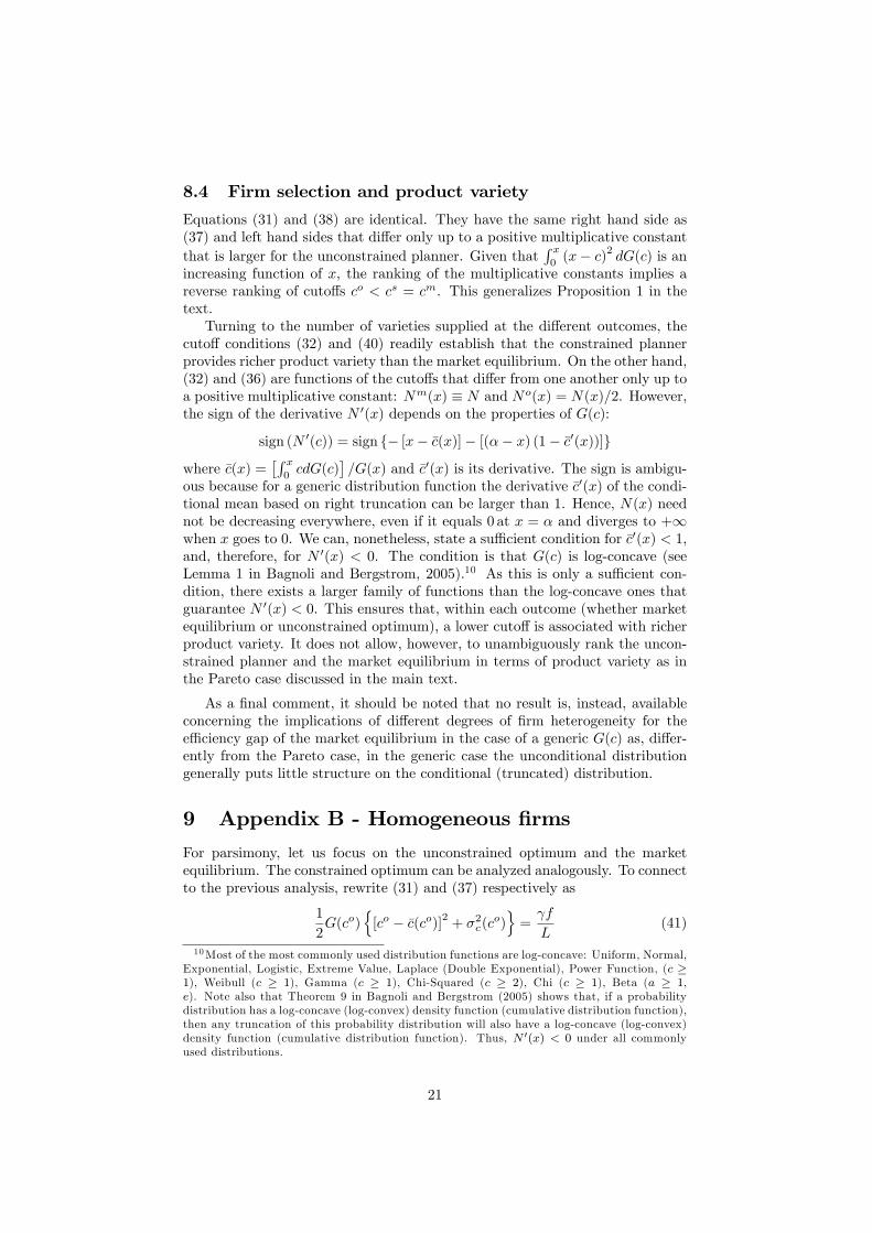
Equations (31) and (38) are identical. They have the same right hand side as(37) and left hand sides that di¤er only up to a positive multiplicative constantthat is larger for the unconstrained planner. Given that

R x0(x� c)2 dG(c) is an

increasing function of x, the ranking of the multiplicative constants implies areverse ranking of cuto¤s co < cs = cm. This generalizes Proposition 1 in thetext.Turning to the number of varieties supplied at the di¤erent outcomes, the

cuto¤ conditions (32) and (40) readily establish that the constrained plannerprovides richer product variety than the market equilibrium. On the other hand,(32) and (36) are functions of the cuto¤s that di¤er from one another only up toa positive multiplicative constant: Nm(x) � N and No(x) = N(x)=2. However,the sign of the derivative N 0(x) depends on the properties of G(c):

sign (N 0(c)) = sign f� [x� �c(x)]� [(�� x) (1� �c0(x))]g

where �c(x) =�R x0cdG(c)

�=G(x) and �c0(x) is its derivative. The sign is ambigu-

ous because for a generic distribution function the derivative �c0(x) of the condi-tional mean based on right truncation can be larger than 1. Hence, N(x) neednot be decreasing everywhere, even if it equals 0 at x = � and diverges to +1when x goes to 0. We can, nonetheless, state a su¢ cient condition for �c0(x) < 1,and, therefore, for N 0(x) < 0. The condition is that G(c) is log-concave (seeLemma 1 in Bagnoli and Bergstrom, 2005).10 As this is only a su¢ cient con-dition, there exists a larger family of functions than the log-concave ones thatguarantee N 0(x) < 0. This ensures that, within each outcome (whether marketequilibrium or unconstrained optimum), a lower cuto¤ is associated with richerproduct variety. It does not allow, however, to unambiguously rank the uncon-strained planner and the market equilibrium in terms of product variety as inthe Pareto case discussed in the main text.

As a �nal comment, it should be noted that no result is, instead, availableconcerning the implications of di¤erent degrees of �rm heterogeneity for thee¢ ciency gap of the market equilibrium in the case of a generic G(c) as, di¤er-ently from the Pareto case, in the generic case the unconditional distributiongenerally puts little structure on the conditional (truncated) distribution.

9 Appendix B - Homogeneous �rms

For parsimony, let us focus on the unconstrained optimum and the marketequilibrium. The constrained optimum can be analyzed analogously. To connectto the previous analysis, rewrite (31) and (37) respectively as

1

2G(co)

n[co � �c(co)]2 + �2c(co)

o= f

L(41)

10Most of the most commonly used distribution functions are log-concave: Uniform, Normal,Exponential, Logistic, Extreme Value, Laplace (Double Exponential), Power Function, (c �1), Weibull (c � 1), Gamma (c � 1), Chi-Squared (c � 2), Chi (c � 1), Beta (a � 1,e). Note also that Theorem 9 in Bagnoli and Bergstrom (2005) shows that, if a probabilitydistribution has a log-concave (log-convex) density function (cumulative distribution function),then any truncation of this probability distribution will also have a log-concave (log-convex)density function (cumulative distribution function). Thus, N 0(x) < 0 under all commonlyused distributions.

21

and1

4G(cm)

n[cm � �c(cm)]2 + �2c(cm)

o= f

L(42)

where we have used the following expression for the conditional variance of themarginal cost distribution �2c(x) =

�R x0c2dG(c)

�=G(x)��c(x)2. Without hetero-

geneity, there is no variance in costs (�2c = 0), all entrants produce (G(cm) = 1),

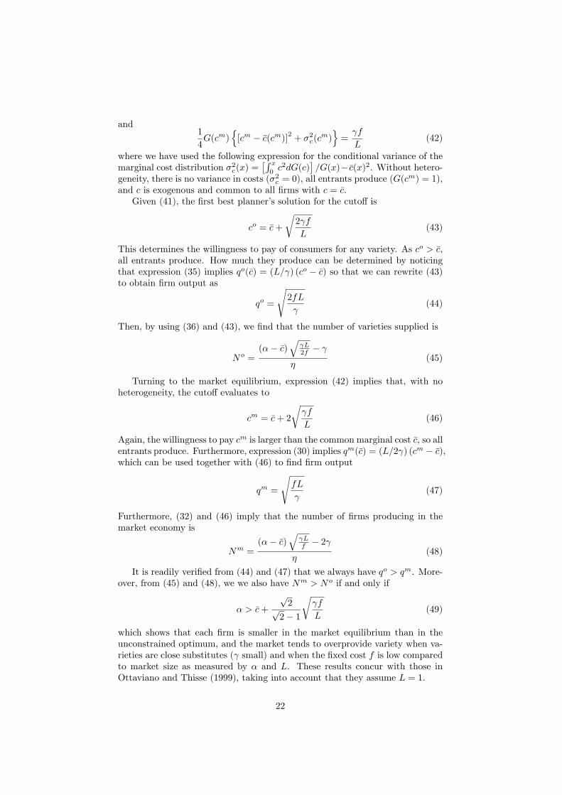
and c is exogenous and common to all �rms with c = �c.Given (41), the �rst best planner�s solution for the cuto¤ is

co = �c+

r2 f

L(43)

This determines the willingness to pay of consumers for any variety. As co > �c,all entrants produce. How much they produce can be determined by noticingthat expression (35) implies qo(�c) = (L= ) (co � �c) so that we can rewrite (43)to obtain �rm output as

qo =

s2fL

(44)

Then, by using (36) and (43), we �nd that the number of varieties supplied is

No =(�� �c)

q L2f �

�(45)

Turning to the market equilibrium, expression (42) implies that, with noheterogeneity, the cuto¤ evaluates to

cm = �c+ 2

r f

L(46)

Again, the willingness to pay cm is larger than the common marginal cost �c, so allentrants produce. Furthermore, expression (30) implies qm(�c) = (L=2 ) (cm � �c),which can be used together with (46) to �nd �rm output

qm =

sfL

(47)

Furthermore, (32) and (46) imply that the number of �rms producing in themarket economy is

Nm =(�� �c)

q Lf � 2

�(48)

It is readily veri�ed from (44) and (47) that we always have qo > qm. More-over, from (45) and (48), we we also have Nm > No if and only if

� > �c+

p2p

2� 1

r f

L(49)

which shows that each �rm is smaller in the market equilibrium than in theunconstrained optimum, and the market tends to overprovide variety when va-rieties are close substitutes ( small) and when the �xed cost f is low comparedto market size as measured by � and L. These results concur with those inOttaviano and Thisse (1999), taking into account that they assume L = 1.

22

10 Appendix C - Heterogeneity and ine¢ ciency

10.1 Equilibrium vs. optimum

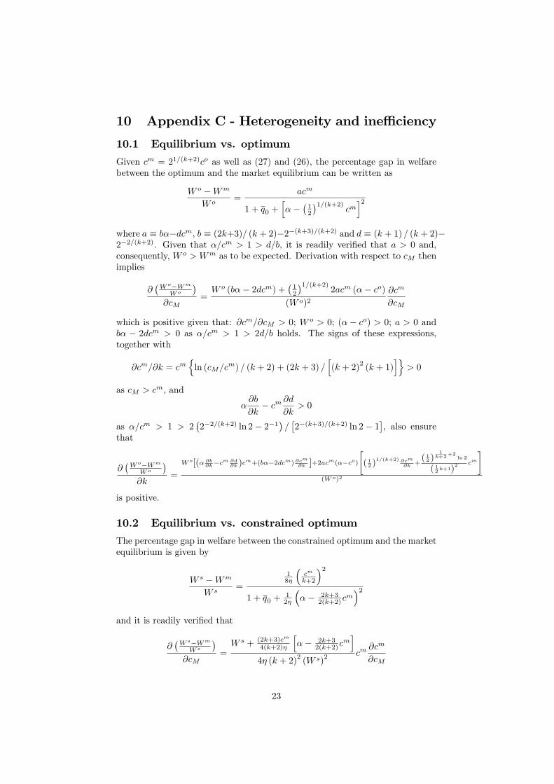
Given cm = 21=(k+2)co as well as (27) and (26), the percentage gap in welfarebetween the optimum and the market equilibrium can be written as

W o �Wm

W o=

acm

1 + q0 +h��

�12

�1=(k+2)cmi2

where a � b��dcm, b � (2k+3)= (k + 2)�2�(k+3)=(k+2) and d � (k + 1) = (k + 2)�2�2=(k+2). Given that �=cm > 1 > d=b, it is readily veri�ed that a > 0 and,consequently, W o > Wm as to be expected. Derivation with respect to cM thenimplies

@�W o�Wm

W o

�@cM

=W o (b�� 2dcm) +

�12

�1=(k+2)2acm (�� co)

(W o)2@cm

@cM

which is positive given that: @cm=@cM > 0; W o > 0; (�� co) > 0; a > 0 andb� � 2dcm > 0 as �=cm > 1 > 2d=b holds. The signs of these expressions,together with

@cm=@k = cmnln (cM=c

m) = (k + 2) + (2k + 3) =h(k + 2)

2(k + 1)

io> 0

as cM > cm, and

�@b

@k� cm @d

@k> 0

as �=cm > 1 > 2�2�2=(k+2) ln 2� 2�1

�=�2�(k+3)=(k+2) ln 2� 1

�, also ensure

that

@�W o�Wm

W o

�@k

=

W o[(� @b@k�c

m @d@k )c

m+(b��2dcm) @cm@k ]+2acm(��co)

24( 12 )1=(k+2) @cm@k +( 12 )

1k+2

+2ln 2

( 12 k+1)2 cm

35(W o)2

is positive.

10.2 Equilibrium vs. constrained optimum

The percentage gap in welfare between the constrained optimum and the marketequilibrium is given by

W s �Wm

W s=

18�

�cm

k+2

�21 + q0 +

12�

��� 2k+3

2(k+2)cm�2

and it is readily veri�ed that

@�W s�Wm

W s

�@cM

=W s + (2k+3)cm

4(k+2)�

h�� 2k+3

2(k+2)cmi

4� (k + 2)2(W s)

2 cm@cm

@cM

23

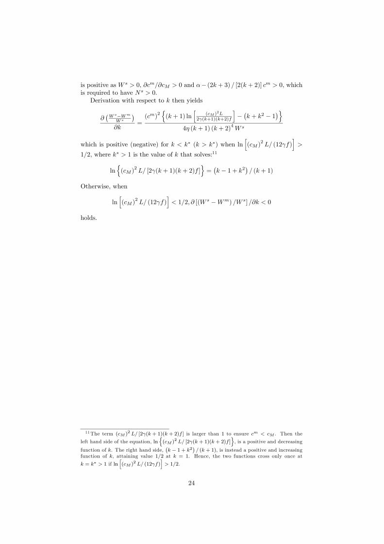
is positive as W s > 0, @cm=@cM > 0 and �� (2k + 3) = [2(k + 2)] cm > 0, whichis required to have Ns > 0.Derivation with respect to k then yields

@�W s�Wm

W s

�@k

=(cm)

2n(k + 1) ln

h(cM )

2L2 (k+1)(k+2)f

i��k + k2 � 1

�o4� (k + 1) (k + 2)

4W s

which is positive (negative) for k < k� (k > k�) when lnh(cM )

2L= (12 f)

i>

1=2, where k� > 1 is the value of k that solves:11

lnn(cM )

2L= [2 (k + 1)(k + 2)f ]

o=�k � 1 + k2

�= (k + 1)

Otherwise, when

lnh(cM )

2L= (12 f)

i< 1=2; @ [(W s �Wm) =W s] =@k < 0

holds.

11The term (cM )2 L= [2 (k + 1)(k + 2)f ] is larger than 1 to ensure cm < cM . Then the

left hand side of the equation, lnn(cM )

2 L= [2 (k + 1)(k + 2)f ]o, is a positive and decreasing

function of k. The right hand side,�k � 1 + k2

�= (k + 1), is instead a positive and increasing

function of k, attaining value 1=2 at k = 1. Hence, the two functions cross only once at

k = k� > 1 if lnh(cM )

2 L= (12 f)i> 1=2.

24

CENTRE FOR ECONOMIC PERFORMANCE

Recent Discussion Papers

1205 Alberto Galasso

Mark Schankerman

Patents and Cumulative Innovation: Causal

Evidence from the Courts

1204 L Rachel Ngai

Barbara Petrongolo

Gender Gaps and the Rise of the Service

Economy

1203 Luis Garicano

Luis Rayo

Relational Knowledge Transfers

1202 Abel Brodeur Smoking, Income and Subjective Well-Being:

Evidence from Smoking Bans

1201 Peter Boone

Ila Fazzio

Kameshwari Jandhyala

Chitra Jayanty

Gangadhar Jayanty

Simon Johnson

Vimala Ramachandrin

Filipa Silva

Zhaoguo Zhan

The Surprisingly Dire Situation of Children’s

Education in Rural West Africa : Results

fromt he CREO Study in Guinea-Bissau

1200 Marc J. Melitz

Stephen J. Redding

Firm Heterogeneity and Aggregate Welfare

1199 Giuseppe Berlingieri Outsourcing and the Rise in Services

1198 Sushil Wadhwani The Great Stagnation: What Can

Policymakers Do?

1197 Antoine Dechezleprêtre Fast-Tracking 'Green' Patent Applications:

An Empirical Analysis

1196 Abel Brodeur

Sarah Flèche

Where the Streets Have a Name: Income

Comparisons in the US

1195 Nicholas Bloom

Max Floetotto

Nir Jaimovich

Itay Saporta-Eksten

Stephen Terry

Really Uncertain Business Cycles

1194 Nicholas Bloom

James Liang

John Roberts

Zhichun Jenny Ying

Does Working from Home Work? Evidence

from a Chinese Experiment

1193 Dietmar Harhoff

Elisabeth Mueller

John Van Reenen

What are the Channels for Technology

Sourcing? Panel Data Evidence from German

Companies

1192 Alex Bryson

John Forth

Minghai Zhou

CEO Incentive Contracts in China: Why Does

City Location Matter?

1191 Marco Bertoni

Giorgio Brunello

Lorenzo Rocco

When the Cat is Near, the Mice Won't Play:

The Effect of External Examiners in Italian

Schools

1190 Paul Dolan

Grace Lordan

Moving Up and Sliding Down: An Empirical

Assessment of the Effect of Social Mobility

on Subjective Wellbeing

1189 Nicholas Bloom

Paul Romer

Stephen Terry

John Van Reenen

A Trapped Factors Model of Innovation

1188 Luis Garicano

Claudia Steinwender

Survive Another Day: Does Uncertain

Financing Affect the Composition of

Investment?

1187 Alex Bryson

George MacKerron

Are You Happy While You Work?

1186 Guy Michaels

Ferdinand Rauch

Stephen J. Redding

Task Specialization in U.S. Cities from 1880-

2000

1185 Nicholas Oulton

María Sebastiá-Barriel

Long and Short-Term Effects of the Financial

Crisis on Labour Productivity, Capital and

Output

1184 Xuepeng Liu

Emanuel Ornelas

Free Trade Aggreements and the

Consolidation of Democracy

1183 Marc J. Melitz

Stephen J. Redding

Heterogeneous Firms and Trade

1182 Fabrice Defever

Alejandro Riaño

China’s Pure Exporter Subsidies

1181 Wenya Cheng

John Morrow

Kitjawat Tacharoen

Productivity As If Space Mattered: An

Application to Factor Markets Across China

1180 Yona Rubinstein

Dror Brenner

Pride and Prejudice: Using Ethnic-Sounding

Names and Inter-Ethnic Marriages to Identify

Labor Market Discrimination

The Centre for Economic Performance Publications Unit

Tel 020 7955 7673 Fax 020 7404 0612

Email info@cep.lse.ac.uk Web site http://cep.lse.ac.uk