Catastrophic Risk and Credit Markets

Mark J. Garmaise

and Tobias J. Moskowitz∗

ABSTRACT

We provide a model of the effects of catastrophic risk on real estate financing and prices and

demonstrate that insurance market imperfections can restrict the supply of credit for catastrophe-susceptible properties. Using unique micro-level data, we find that earthquake risk decreased

commercial real estate bank loan provision by 22 percent in California properties in the 1990’s.The effects are more severe in African-American neighborhoods. We show that the 1994 Northridgeearthquake had only a short-term disruptive effect. Our basic findings are confirmed for hurricane

risk, and our model and empirical work have implications for terrorism and political perils.

∗UCLA Anderson School and Graduate School of Business, University of Chicago and NBER, respectively. We thank

Bing Han, Robert Novy-Marx and participants at the Vail Real Estate Research Conference for helpful comments.

We thank AIR Worldwide Corporation, Guy Carpenter and COMPS.com for providing data. Moskowitz thanks the

Center for Research in Security Prices and the Neubauer Family Faculty Fellowship for financial support.

Correspondence to: Mark Garmaise, UCLA Anderson School, 110 Westwood Plaza, Los Angeles, CA 90095-1484.

E-mail: mark.garmaise@anderson.ucla.edu.

Catastrophic events can dramatically affect the well-being of people throughout entire regions.

Episodes such as September 11, 2001, the December 26, 2004 tsunami in Asia, and Hurricane

Katrina in August 2005 highlight the risks borne by individuals, particularly those with limited

financial resources. Financial markets can help to manage these risks by playing two crucial roles.

First, markets provide a mechanism through which risk is allocated efficiently. Second, financial

markets can serve as a stable source of funding during post-catastrophe periods. Little is known,

however, about how well financial markets perform these functions. In this paper, we provide

a model of the effects of catastrophe risk on the financing and pricing of properties and find

corroborating evidence for the model using unique micro-level data on earthquake risk (the average

annual loss due to earthquake damage) and credit.

We show that apparent inefficiencies in the supply of catastrophe insurance have a substan-

tial ongoing distortionary effect on bank credit markets. In particular, our results indicate that

earthquake risk reduced the provision of bank financing by approximately 12 percentage points (22

percent) in California commercial real estate loan markets in the 1990’s. We also find, however, that

the large 1994 Northridge earthquake affected the market for only about three months following the

event. These results suggest that while catastrophic risk may not be generally allocated efficiently,

the additional distortions caused by even significant catastrophic events are quite short-lived. Our

work highlights general features of catastrophic risk markets that are shared by a variety of perils

including hurricane, terrorism, and political risks. We extend our basic findings to hurricane risk

and argue that our results imply that, in the absence of well-functioning insurance markets, terror-

ism risk is likely to discourage bank financing of properties in high profile U.S. cities and political

risk may impede the development of corporate debt markets in emerging economies.

Our model examines the potential distortionary effect of catastrophe risk on credit markets.1

We emphasize that bank financing of catastrophe-susceptible properties is likely to be inefficient.

Banks do not specialize in monitoring whether property owners are implementing all positive NPV

safety-enhancing investments. In the presence of a bank loan, due to a risk-shifting motive, owners

may prefer not to make these investments. Insurers, by contrast, are expert in monitoring the

execution of safety-increasing improvements, so the presence of a well-functioning insurance market

can ameliorate the problems in bank financing of properties at risk of a catastrophe. Insurance

1The management of catastrophic risk has been the theme of a recent stream of research analyzing insurance(Jaffee and Russell, 1997, Niehaus, 2002, Zanjani, 2002), reinsurance (Froot and O’Connell, 1997, Froot, 2001) andcatastrophic-loss derivatives (Cummins, Lalonde and Phillips, 2004).

1

markets, however, may be imperfectly competitive due to capital constraints (Winter, 1994 and

Gron, 1994) or information asymmetries (Cummins and Danzon, 1997). Froot (2001) contends that

catastrophe insurance, in particular, is over-priced and in relatively short supply due to capital

market imperfections and market power enjoyed by the relatively small number of catastrophe

reinsurers. We show that a poorly functioning catastrophe insurance market will lead to less

bank financing of catastrophe-susceptible properties, reduced market participation by less-wealthy

investors and incomplete insurance coverage. Inefficiencies in the catastrophe insurance market will

also derail positive NPV investments by investors who require loans.

To test the theory, we perform an empirical analysis using unique data on catastrophic earth-

quake risk and commercial property loan contracts and prices in the U.S. in the 1990s. Using data

from Standard and Poor’s (S&P) ratings of commercial mortgage-backed securities (CMBS), we

first show that only 35% of properties in earthquake zones carry earthquake insurance and the prob-

ability that insurance is purchased is increasing in earthquake risk. These findings are consistent

with our model and suggest that earthquake insurance is inefficiently supplied.

To analyze the impact of earthquake risk on the provision of finance, we match property-level

financing and price information on commercial property transactions from COMPS.com with a

unique data set of micro-level earthquake risks, provided by AIR Worldwide Corporation (AIR).

We find that increased earthquake risk dramatically reduces the likelihood that a property will be

financed with bank debt, controlling for census tract fixed effects. Within-neighborhood identifi-

cation is empirically feasible because differences in soil conditions create highly localized variation

in the effects of earthquakes; the AIR earthquake risks reflect both fault location and detailed soil

condition data. Our results suggest that in Los Angeles county, for example, the median quake

risk reduces the probability of bank financing by over 20 percent, indicating that imperfections in

the allocation of catastrophe risk can disrupt bank credit markets in a manner consistent with the

theory.

We then examine the cross-section of properties to determine if these effects are stronger for

different groups of buyers or properties in ways predicted by the theory. We show that when insur-

ance firms (insurers or insurance brokers) purchase properties, earthquake risk has a significantly

smaller affect on the probability that a bank loan is used to finance the property than it does for

other buyers. Since insurance firms have better access to earthquake insurance, they are not as

severely affected by the general lack of supply. As predicted by the model, the use of bank credit

2

by insurance firms is thus less distorted by the presence of earthquake risk. We also find that

properties in areas with large African-American populations are especially unlikely to be financed

with bank debt in the presence of quake risk, controlling for the overall provision of bank loans.

Earthquake insurance may be particularly hard to obtain in African-American neighborhoods for

a variety of reasons, which would create more serious credit distortions linked to earthquake risk

in these areas.

If there is a limited supply of earthquake insurance, intermediaries such as property brokers

who repeatedly participate in the market may be able to cultivate cooperative relationships with

insurance firms and facilitate their clients’ access to insurance and hence bank loans. Consistent

with this idea, we show that deals involving property brokers are especially more likely to receive

bank financing in high-quake-risk areas. This result continues to hold when we instrument for

property broker presence using the local thickness of the market for a particular property (brokers

are used less often for properties that are traded in thick markets). Our final cross-sectional

result is that quake risk reduces the probability of bank financing particularly for older buildings.

Earthquakes are likely to cause greater damage to older properties, so quake risk is probably most

important for these buildings.

While we find strong evidence linking quake risk to bank loan provision, we show that the

probability of seller financing is not strongly tied to quake risk. Although sellers face the same risk-

shifting incentive as banks, sellers, unlike banks, have excellent information about the property

as previous owners of the property and are thus capable of ensuring that the safety-improving

investments are undertaken. To further corroborate this story we show that when the seller’s

information is less relevant (e.g., for properties slated for development where the property is going

to change dramatically) or less extensive (e.g., seller’s with very short tenure in the property), the

risk-shifting motive dominates and we get the same results linking quake risk to loan provision for

these sellers as we do for banks.

Earthquake risk also influences the characteristics of buyers and financing banks. We find that

in the pool of non-corporate buyers, the purchasers of high quake risk properties come from zip

codes with higher median home values. This evidence supports the implication of the model that

properties with higher catastrophic risks will be purchased by buyers who are wealthier on average.

We also show that local banks are relatively more likely to finance high quake risk properties,

which is consistent with the underlying premise of the theory that monitoring (better performed

3

by nearby banks) is more important for properties with greater catastrophe risk.

In addition to its disruptive influence on real estate financing, our model shows that catastrophic

risk has a direct effect on asset pricing: properties at risk for earthquake damage should have lower

prices, reflecting their increased potential for physical destruction. We find, however, that it is only

in larger deals that buyers consistently apply greater discounts to properties with higher quake risk

than others in the same census tract. It may be that the indirect financing effects we model are

most important for larger transactions.

We also examine the aftermath of one of the largest earthquakes in recent history, the January,

1994, Northridge earthquake, which caused an estimated $42 billion in damages ($14 billion of

which was insured). The Northridge quake caused a negative shock to the supply of earthquake

insurance, and we study the impact and longevity of this shock. Our analysis shows that, consistent

with the theory, properties with high quake risk were especially unlikely to be financed with bank

loans in the period directly following the Northridge quake. The insurance supply shock generated

by the quake further exacerbated the reduced provision of bank loans to high catastrophe risk

properties. The duration of this effect was approximately 3 months. We demonstrate that local

banks were less likely to make loans to high-quake-risk properties in the period after the event. We

also find that, as the model predicts, bank-financed transactions were concentrated in lower-risk

properties following the Northridge quake, while cash-financed transaction displayed no such shift.

The effects from the earthquake were short-term and had no significant long-term impact on the

pricing or financing of catastrophe risk.

Our model emphasizes general features of catastrophic risk markets: lack of bank specializa-

tion in monitoring safety-improving investments and restricted supply of catastrophe insurance.

These features are shared by an assortment of catastrophic perils including earthquake, hurricane,

terrorism and political risks. Earthquake data is particularly suitable for testing the theory for

two reasons. First, risk assessors can generate objective quantitative measures of earthquake risk.

Second, earthquake risk varies at the highly local level, which enables the use of census tract fixed

effects to control for unobservables.

To explore the broader implications of our findings, we extend the empirical work to an analysis

of hurricane risk, which shares many of the features of earthquake peril. While the properties in

our sample have relatively low exposure to hurricanes, we do find evidence that properties with

higher hurricane risk than others in the same zip code tend to receive less bank financing. This

4

effect is magnified when the price of catastrophe insurance is high. These results provide further

evidence for the theory using a second catastrophic risk setting.

We argue that the supply of terrorism risk insurance, which has recently become a subject of

intense interest, is likely to be even more restricted than that of natural disaster insurance for three

reasons. First, terrorism risk is particularly difficult to evaluate and this ambiguity can hamper the

supply of insurance (Hogarth and Kunreuther, 1985). Second, terrorism is endogenous, so markets

set up to allocate terrorism risk may be manipulated (Poteshman, 2006). Third, the damages

from a catastrophic act of terrorism may be may greater than those caused by natural phenomena.

Consequently, the effects we document for earthquake risk may be even more severe for terrorism

risk. A decision by the government to decline to support the terrorism insurance market (for

example, by refusing to renew the Terrorism Risk Insurance Act) may have important consequences.

Our work suggests that in the absence of government-subsidized terrorism insurance, high profile

and high density areas such as the downtowns of large U.S. cities would likely experience both a

significant shift away from bank financing of properties and market exit by less well-capitalized

investors. Also, reconstruction after a terrorism incident would likely be hampered by limited

supply of bank credit in the immediate period following an event.

Political risk such as nationalization or currency controls, which are typically of greatest concern

in emerging economies, also exhibit properties similar to those of other catastrophic perils: huge

potential losses and lack of bank skill in monitoring and liquidating affected investments. Political

risk, like terrorism, also faces the problem of uncertain hazard assessment, and the supply of

political risk insurance is quite limited (Hamdani et al., 2005). Our findings indicate that less

well-capitalized firms that require financing will be significantly more likely to invest in emerging

markets if there is a sufficient supply of fairly priced political risk insurance, and by extension will

encourage the issuance of emerging market corporate bonds.

The remainder of the paper is organized as follows. Section I describes our theoretical model

of the pricing and financing of catastrophe risk. Section II details the commercial real estate and

earthquake data. Section III investigates the effects of earthquake risk on real estate financing and

prices. Section IV analyzes the impact of the Northridge quake. In Section V we consider the

implications of our findings for hurricane, terrorism, and political risks. Section VI concludes.

5

I. Model

We develop a theory of the pricing and financing of properties in the presence of catastrophic risk.

We begin with a simple model of identical investors all of whom are financially unconstrained.

We then consider the presence of an investor with a higher valuation (or private benefits), who is

potentially financially constrained. We will argue that banks are inefficient at financing catastrophe-

susceptible properties, but that this inefficiency can be ameliorated by insurers. We conclude the

model by examining the implications of imperfections in the supply of catastrophic risk insurance

for the financing of properties.

A. Unconstrained investors

For simplicity, consider a property generating cash flow Ct each period t with an associated dis-

count rate r for these cash flows. We assume that Ct+1 = αt+1Ct, where the {αs} are mutually

independent and E[αs] = 1 for all s. This implies that E[Ct+1|Ct] = Ct. Properties differ in

their susceptibility to catastrophic (e.g., earthquake or hurricane) damage.2 For each property, a

parameter p describes both the probability that the property will be affected by a catastrophe and

the severity of any such catastrophe. Each period t with probability p there is no catastrophe.

With probability 1− p a catastrophe occurs and leaves the property with a salvage value that is a

fraction Rt of the undamaged property value Vt, where Rt ∈ [0, 1] is a random variable.3 We also

assume for simplicity that the current cash flows are lost, though the results hold for fractional

cash flow losses as well. We presume that the {Rt} are identically and independently distributed,

with common mean E[R] ∈ [0, 1). We refer to (1− p) as the catastrophic risk of the property.

In the event of a catastrophe, we assume that instantaneous repairs costing (1 − Rt)Vt must

be undertaken before the property will generate future cash flows.4 The net present value of these

repairs when there is a catastrophe is N (Vt, Rt) = VtRt ≥ 0. We assume that catastrophe risk

(both frequency and severity) is uncorrelated with economy-wide financial wealth (as argued by

2The model applies to all cases of damage risk (e.g., fire), but, as we will discuss, the insurance supply distortionsthat play a role in the theory are most plausible for catastrophe risk.

3The scientific literature on earthquakes has established the Gutenberg-Richter frequency magnitude law, whichstates that magnitudes are governed by an exponential distribution, with relatively little variation across locations inthe exponential parameter (Kagan, 1997). While the frequency of earthquakes can vary substantially across regions,the distribution of earthquake severities, given an event, is actually quite stable across areas. This result suggeststhat modelling the severity of the damage as independent of its frequency is reasonable. Hurricanes, cyclones andfloods also exhibit similar frequency-magnitude patterns (MacDonald, 2000).

4Assuming that a catastrophe also changes the future cash flows generated by a property has no effect on theresults.

6

Froot, 2001) and that investors are well diversified and financially unconstrained. Investors will

always undertake the repairs, since N ≥ 0.

The average annual loss q is defined as q = (1 − p)(1 − E[R]), which is the expected fraction

of property value that is destroyed by the catastrophe in each period. The average annual loss

is sometimes described as the catastrophe premium (Ruttener, Liechti and Eugster, 1999). Using

standard arguments, we show in the Appendix that Vt = pCt

r+q . The cap rate (ratio of earnings to

price) is thus given by r+qp

.

The above straightforward discrete time model yields the basic intuitions necessary for our tests.

Duffie and Singleton (1999) provide a general theoretical treatment of the pricing of assets in the

presence of exogenous value-destruction risk.

Our first result describes the pricing effects of catastrophe risk: properties subject to catastrophe

risk sell for lower multiples of their current cash flows.

Result 1. The derivative of the cap rate with respect to the average annual loss is at least one.

The proofs of all Results are given in the Appendix.

B. Constrained Investors and Differential Valuations

We now introduce two modifications to the base model. First, for a given property with current

value Vs in period s, with probability ζ there is an investor who can generate an additional value

b ≥ 0 from purchasing the property and managing it for the next period. This additional valuation

might arise from a positive net present value investment known only to the investor or from a

private benefit. For simplicity we will assume that b is a private benefit, though our results are not

sensitive to that assumption. The realization of b is known to the investor.

Second, we assume that this investor has wealth wL < Vs with probability l ∈ (0, 1). With

probability (1− l), the investor has wealth wH > Vs. That is, we introduce financially constrained

investors who do not have enough cash to purchase the property. The investor with a private

benefit pays only the market value Vs if he purchases the property, just as he would if the property

were sold in a public auction.

B.1. Inefficiency of Bank Financing in the Absence of Insurance

We begin by assuming that no catastrophic insurance is available. Constrained investors will require

a bank loan. Banks have unlimited capital, and we assume that the banking sector is competitive;

our focus is on credit market distortions that are related to catastrophic risk, rather than general

7

credit market distortions. We presume that the bank financing of catastrophe-susceptible properties

is inefficient.

We model this inefficiency as arising from the fact that banks do not specialize in monitoring

whether a property owner is implementing all positive net present value (NPV) damage-reducing

safety investments. In the presence of bank debt, an owner may prefer to forgo these investments,

since they reduce the risk of the property, thereby increasing the value of the bank loan and

potentially decreasing the value of the owner’s equity (Smith and Warner, 1979). The bank financing

of catastrophe-susceptible properties will thus lead to inefficient underinvestment in positive NPV

safety enhancement projects.

Consider a property with value Vs that may experience a catastrophe with probability (1− p).

The argument just given suggests that if an investor purchases the property with w in equity and

a bank loan of Vs − w ≥ 0, then the inefficiency associated with bank financing will result in value

destruction, which we denote by loss(w, Vs, p). We will assume that the value destruction satisfies

two properties:

Property 1: loss(w, Vs, p) is decreasing in p and w

Property 2: loss(w, Vs, p) > 0 if Vs > w and p < 1, but loss(w, Vs, p) = 0 if Vs = w or if p = 1.

The first property captures the idea that the expected efficiency losses generated by the bank’s

lack of information and inability to monitor damage prevention projects are more severe both when

the catastrophe risk is high and when the equity provided by the investor is low. The second

property specifies that if there is no catastrophe risk, or if the project is wholly equity financed,

then there is no value destruction. The presence of some catastrophe risk combined with bank

financing always leads to a measure of inefficiency, however small.

In the appendix we provide a formal model of imperfect bank information about safety invest-

ments and the resultant risk-shifting by property owners. We show that this model yields the two

properties detailed above. What is central to our paper, however, is simply the idea that bank

financing of catastrophe-prone properties is inefficient. This inefficiency might also be generated by

a different model in which banks do not specialize in the evaluation or remediation of catastrophic

damage, which may lead to inefficient foreclosure and liquidation by banks of properties damaged

in catastrophes.5

5We presented a formal model of this idea in a previous draft.

8

We define ΠB(w, Vs, p) to be the net present value received by this investor if he invests w ≤ Vs

in cash and borrows Vs − w in order to purchase a property with catastrophe frequency (1 − p).

The value of the investor’s equity claim is equal to the value Vs of the property minus the value

of the bank’s debt claim minus any value destroyed in inefficient liquidation. Credit markets are

competitive, so the net present value of the investor’s investment is therefore equal to his private

benefit minus the value destroyed in inefficient liquidation. Since not investing is always an option,

we have

ΠB(w, Vs, p) = max{b − loss(w, Vs, p), 0}.

B.2. Insurance Market

We now introduce the possibility of catastrophe insurance. We assume there are two potential

insurers who offer full insurance contracts (covering all cash flow and property value losses), though

our results are not sensitive to either of these assumptions. Insurers differ from banks in that

they know which safety-enhancing investments are positive NPV, and insurers can therefore offer

contracts that are contingent on the owner undertaking these investments. Since these investments

are positive NPV, optimal insurance agreements will incentivize owners to make them, in exchange

for lower premia. The provision of insurance thus removes the source of inefficiency associated with

the bank financing of properties subject to catastrophe risk.6

We presume, however, that the catastrophe insurance market is potentially imperfectly com-

petitive. Imperfections may arise from a number of sources. Winter (1994) and Gron (1994) show

that a combination of correlated insured losses, restrictions on the default probabilities permitted

for insurers, and costly external financing leads to a capacity-constrained and imperfectly com-

petitive insurance industry. Cummins and Danzon (1997) argue that policyholder switching costs,

generated by learning over time both by policyholders about insurers and vice versa, can deter

entry by new insurers. Froot (2001) describes the role of market power and capital constraints

in the reinsurance industry. The infrequency of catastrophic events may exacerbate information

6Shown formally in the Appendix. One might ask why banks do not acquire the information expertise of insurers.It may be the case that acquiring such expertise involves large fixed costs that can only be justified by engagingin a full business of underwriting policies. That is, a bank would have to use this expertise as widely as insurancecompanies do, not just for properties secured by the bank’s loans. Why, then, do banks not simply merge withinsurers? Until the passage of the Gramm-Leach-Bliley Act of 1999, just shortly after the close of our sample period,this was legally difficult. Even after the passage of this act, however, such mergers carry with them the usual costs(e.g., loss of focus, agency problems) associated with universal banking in general. DeLong (2001) provides someevidence that diversifying mergers by U.S. banks do not create value, but Cybo-Ottone and Murgia (2000) show thatEuropean bank-insurance mergers do generate positive announcement effects.

9

asymmetries between potential investors and insurers, because it is difficult for outsiders to assess,

in the absence of a catastrophe, how careful an insurer is offering coverage. This difficulty may

serve to particularly constrict the flow of capital to potential entrants in the catastrophic insurance

market.

We assume that each insurer is able to make a bid on any given catastrophe insurance contract

with probability n ∈ [0, 1]. Whether an insurer can bid is independent of what happens to his

competitor. Each insurer who can bid proposes a price for full insurance, and the property owner

may select the lower bid or choose not to purchase insurance. We describe the insurance market as

perfectly competitive if n = 1 and imperfectly competitive otherwise. The fair value of insurance

is the market value of the insurance payout.7

We describe the bid of an insurer by viewing it as a mark-up, mar, over the fair value of the

insurance. If both insurers bid for the contract, the unique equilibrium is for each to set mar = 0.

If only one insurer bids, he will choose mar to maximize his expected profits. Financially uncon-

strained investors will never pay a positive premium for insurance, since they need not finance with

a loan and will therefore never suffer the inefficiencies of bank financing, so the insurer maximizes

the profits he realizes from selling to constrained investors. Any bid mar > wL will be rejected,

since the investor has insufficient resources to pay this amount. The bid is also rejected if it is

less expensive for the investor to purchase the property without insurance: mar > loss(wL, Vs, p).

Lastly, if mar > b, the investor will prefer to forego the property purchase rather than buying

insurance.

Insurers do not know the realization of the private benefit b, but they know its associated cdf

Fb and pdf fb. We assume that Fb satisfies the MHR property. We denote by b∗ the solution to the

following maximization problem:

maxy≥0

[y (1 − Fb(y))] . (1)

The MHR property guarantees that b∗ is unique. An insurer bidding alone will set mar =

min{b∗, wL, loss(wL, Vs, p)}. As a property’s catastrophic risk increases, Property 1 indicates that

the option of financing with a bank loan becomes increasingly unattractive. As catastrophe risk

increases, two things occur in an imperfectly competitive insurance market: A single insurer bidding

will charge a higher mark-up and, if no insurer bids, the investor is less likely to proceed with the

7For simplicity, we ignore the costs associated with damage assessment and monitoring. Including these costs doesnot affect the results.

10

purchase. Both of these effects reduce the frequency of bank-financed transactions. If the insurance

market is perfectly competitive, insurance is always supplied at zero mark-up.

Result 2. If the insurance market is imperfectly (perfectly) competitive, the probability that

a transaction is financed with bank debt is decreasing (independent) in the property’s catastrophic

risk.

In an imperfectly competitive insurance market, expensive insurance premiums combined with

the inefficiency of bank financing in the absence of insurance together discourage less wealthy

investors from purchasing properties with high catastrophic risk. Even though the credit mar-

ket itself is competitive, the insufficient supply of insurance leads to distortions in the financing

of catastrophe-susceptible properties. Investors with substantial wealth purchase the properties

without insurance or a loan.

Result 3. If the insurance market is imperfectly (perfectly) competitive, the average wealth of

the purchasing investor is increasing (independent) in the property’s catastrophic risk.

As catastrophic risk increases, Property 1 implies that fewer financially constrained investors

will buy the property without insurance. In an imperfect insurance market, if insurance is offered,

the mark-up demanded will increase with catastrophic risk, but in such a way that the investor

will still prefer to buy insurance rather than purchasing the property without it. The net effect is

that as catastrophic risk increases, more of the bank-financed transactions will carry insurance. In

a perfect insurance market, insurance will always be purchased because it avoids the inefficiencies

of bank financing.

Result 4. If the insurance market is imperfectly competitive, the probability that a bank-financed

transaction is accompanied with insurance is increasing in the property’s catastrophic risk. If the

insurance market is perfectly competitive, all bank-financed purchases of properties with positive

catastrophic risk will be accompanied with insurance.

As catastrophic risk increases, in an imperfect insurance market, two classes of investors elect

not to purchase the property. First, constrained investors who receive no insurance bid and find the

cost of financing the property without insurance too high. Second, constrained investors who receive

one bid and find both the insurance bid and the cost of financing the property without insurance

too high. Since it is economically efficient for the investor to always purchase the property, this

suggests that there are social welfare costs arising from imperfections in the insurance market:

Positive net present value projects will be abandoned.

11

Result 5. If the insurance market is imperfectly (perfectly) competitive, the probability of a

transaction is decreasing (independent) in the property’s catastrophic risk.

We also consider the effects of a change in the competitiveness of the insurance market, such

as might arise following a large catastrophic event. As competitiveness decreases, financially con-

strained investors will be unable to purchase affordable insurance and will not be able to make

bank-financed purchases.

Result 6. The probability that a transaction is financed with bank debt is increasing in insurance

market competitiveness n.

An increase in competitiveness will particularly benefit constrained investors considering pur-

chasing high-catastrophe-risk properties. Thus, as competitiveness increases, there should be an

especially large increase in bank-financed purchases of high-risk properties. Unconstrained in-

vestors using cash to make their property purchases will be unaffected by the competitiveness of

the insurance market.

Result 7. The average catastrophic risk of bank-financed transactions is increasing in insurance

market competitiveness n. The average catastrophic risk of all-cash transactions is independent of

insurance market competitiveness n.

In Section III we will test these predictions using empirical data on earthquakes. Clearly, in

practice, the insurance market will not be perfectly competitive. Our empirical results, however,

will examine the importance of this imperfection and quantify its spillover effects on credit markets.

B.3. Seller Financing

After bank loans, the second most common form of debt in commercial real estate markets is seller

financing. Our model does not make unambiguous predictions about the relationship between

seller financing and catastrophe risk. On the one hand, sellers have excellent information about the

properties they are financing, since they previously owned them. Just as we assume that the new

owner is aware of which safety-enhancing investments are positive NPV, it is reasonable to presume

that the previous owner also knows which investments will create value. If that is the case, the sellers

can condition their mortgage terms on these investments being made, precisely as we described for

the insurers. Banks, on the other hand, lack this information, and cannot enforce contract terms of

this kind. Seller financing would therefore not lead to inefficient underinvestment in the presence of

catastrophe risk, since the terms of the seller financing would condition on appropriate maintenance

and investment to protect the property. Hence, the property-specific knowledge of the seller can be

12

used to avoid underinvestment in a manner analogous to the general safety investment knowledge

of the insurer. Seller financing would not be affected by the presence of catastrophe risk (or it

might increase, as it substitutes for bank debt).

The counter argument is that sellers may not be as expert as insurers at monitoring the im-

plementation of safety investments, and hence the frequency of seller financing will be reduced by

catastrophe risk, just as it would be for bank financing. Given the theoretical indeterminacy of this

question, we leave the relationship between seller financing and catastrophe risk to be considered

as an empirical issue.

II. Data and Summary Statistics

We briefly describe the variety of data sources used in the paper.

A. Transaction-level data from the U.S. commercial real estate market

Our transaction-level commercial real estate sample consists of 32,618 transactions drawn from

across the U.S. over the period January 1, 1992 to March 30, 1999 compiled by COMPS.com, a

leading provider of commercial real estate sales data. Garmaise and Moskowitz (2003, 2004) provide

an extensive description of the COMPS database and detailed summary statistics. The data span

11 states: California, Nevada, Oregon, Massachusetts, Maryland, Virginia, Texas, Georgia, New

York, Illinois, and Colorado, plus the District of Columbia.

Commercial properties are grouped into ten mutually exclusive types: retail, industrial, apart-

ment, office, hotel, commercial land, residential land, industrial land, mobile home park and special.

Panel A of Table I reports summary statistics on the properties in our sample. The average (me-

dian) sale price is $2.2 million ($590,000), and there are only 42 transactions involving REITS (less

than 0.2% of the sample). Capitalization rates, defined as current net income on the property

divided by sale price, and property age are also reported.

The COMPS database provides detailed information about specific property transactions, in-

cluding property location, identity and location of market participants, and financial structure.

In particular, COMPS provides eight digit latitude and longitude coordinates of the property’s

location (accurate to within 10 meters).

The COMPS data contain financing information for each property transaction. We focus on the

terms of the loan contract, including interest rates, and the size and presence of loans. As Panel A

13

of Table I indicates, the average loan size (from bank and non-bank institutions) as a fraction of

sale price is over 75%. Bank loans are used in 53% of transactions, vendor-to-buyer (VTB) loans

(i.e., seller financing) are used in 19% of deals and less than 5% of deals involve assumed debt. The

data also contain rich detail on loan terms including the annual interest rate, the maturity of the

loan, whether the loan rate is floating or fixed, whether amortized and the length of amortization,

and whether the loan is subsidized by the Small Business Administration (only 1.3% of loans). The

COMPS data do not, however, include insurance information on properties.

B. Commercial Mortgage-Backed Securities Data

We make use of data on CMBS transactions provided by the S&P RatingsDirect database. This

data provides descriptive details on fifty CMBS transactions over the period 1996 to 1999. Each

CMBS issuance covers multiple properties, as described in Panel B of Table I, and in many cases

information on earthquake risk and insurance is given.

C. Earthquake risk

AIR Worldwide Corporation (AIR) provides detailed data on the earthquake risks associated with

our COMPS properties’ locations (accurate to within 10 meters). AIR is a highly regarded vendor of

estimates for various types of catastrophe risks. Using its proprietary CATStation Hazard Module,

AIR generates location-specific assessments of the expected average annual loss due to earthquake

risk. (Cummins, Lalonde and Phillips, 2004 describe the AIR catastrophe models.) The average

annual loss denotes the fraction of property value that is expected to be destroyed by an earthquake

in any given year. It is expressed as a percentage, and it reflects both the likelihood of an earthquake

and the distribution over potential severities. Property characteristics will also have an effect on

the impact of an earthquake, but the AIR estimates incorporate only location, not structure or

characteristics.8 We use AIR’s estimate of average annual loss as our measure of quake risk.

The AIR earthquake model uses both fault location and detailed soil condition data. Soil

characteristics have a large impact on the way seismic waves are transmitted. Using this data,

the AIR model makes highly localized predictions of average annual loss. For example, the AIR

soil database for the area around the San Francisco Bay has a horizontal resolution of 24 square

meters.9

8AIR does generate structure-specific estimates, but these were not provided to us.9This description of the AIR model is drawn from http://www.air-worldwide.com. The January 1994 Northridge

earthquake caused some revisions to earthquake risk assessments. All the results in the paper are robust to using

14

Panel B of Table I presents summary statistics for AIR earthquake risks. For most properties

in our sample, the average annual loss is described as less than 0.1%, which we code as 0. There

are 9,785 properties with positive quake risks, all located in California, Oregon and a handful of

sites in Massachusetts. Our data include 12,288 properties in California and 9,386 properties in

Los Angeles county.

In many cases the S&P data supplies earthquake risk and insurance data on the properties

securing the CMBS issuance. For properties in earthquake zones (primarily California, but also

including parts of Nevada, Washington, Oregon, Utah and Missouri) the probable maximum loss

(PML) is often specified, along with information about whether the property has earthquake in-

surance. S&P defines the PML to be the expected earthquake damage (expressed as a fraction of

property replacement cost) that has a ten percent chance of being exceeded during a fifty year pe-

riod (Standard and Poor’s, 2003). This measure of earthquake risk is closely related to the average

annual loss. In most cases, the S&P data will specify only whether the PML exceeds a threshold,

typically 20%.

D. The Northridge Earthquake

Our data and sample period also allow us to consider the impact of an actual sizable earthquake,

the Northridge earthquake of January 17, 1994. The Northridge earthquake measured 6.7 on the

Richter scale, caused 57 deaths and was responsible for direct economic damages of approximately

$42 billion (of which $14 billion was insured), according to reliable estimates (Petak and Elahi,

2000). The U.S. Geological Survey (USGS) provides data on the severity of ground motion during

the Northridge quake.10 Specifically, we consider the peak ground acceleration (PGA), which is the

maximum acceleration experienced at a specified location on the earth’s surface during the course

of an earthquake. The PGA is a commonly used metric for earthquake severity, and building codes

often describe requirements for withstanding shaking in terms of horizontal force, which is related

to PGA. Data is provided for points on a grid system, with a distance between grid points of

approximately 1.15 miles on the north-south axis and 0.94 miles on the east-west axis. We match

our property locations to the nearest grid point in order to infer the extent of local PGA. This

process generates PGA estimates for every COMPS property in Los Angeles county. Summary

statistics are given in Panel B of Table I.

only post-January 1994 data.10The data may be found at http://earthquake.usgs.gov/shakemap.

15

E. Crime and Census Data

We also make use of local crime and census data. The crime risk data is provided by CAP Index,

Inc., and vary within census tracts (see Garmaise and Moskowitz (2005) for further details). The

census data come from the 1990 and 2000 U.S. censuses.

III. The Effects of Earthquake Risk on Financing and Prices

Using the earthquake risk and commercial property loan data, we test the hypotheses outlined in

Section I by examining the impact of earthquake risk on financing and prices. We also provide some

general descriptive statistics on the effects of earthquake risk on commercial real estate markets.

The commercial real estate market is a useful laboratory to investigate the role of catastrophe

risks because the loans are typically secured and non-recourse, providing a set of project-specific

financings for which the collateral value is of central importance.

A. Quake risk and insurance

The theory in Section I advanced the argument that an imperfectly competitive catastrophe in-

surance market can impede the supply of credit in the real estate market. Catastrophe insurance

reduces the costs of securing a loan because it encourages owners to make all safety-enhancing

positive NPV investments. If catastrophe insurance is priced at a premium, as suggested by Froot

(2001), then buyers who require a loan will only purchase insurance when the costs of inefficient

bank financing are very high, i.e. for high-quake-risk properties. This idea is captured in Result

4, which states that in imperfectly competitive insurance markets the probability that a bank-

financed transaction is accompanied with insurance is increasing in the property’s catastrophe risk.

In perfectly competitive insurance markets, all bank-financed properties should carry insurance.

Insurance data on individual properties is quite difficult to secure (Squires, O’Connor and Silver,

2001), but the S&P CMBS database provides this information on properties in quake-susceptible

areas as part of its ratings process. The properties in this database have securitized loans, which

make up a significant (and growing) fraction of total commercial mortgage lending during our

sample period.11 Hence, these properties are representative of our larger database on commercial

real estate from COMPS, which does not contain information on quake insurance. Panel C of Table

I shows that for the 482 properties in the S&P CMBS transactions that reside in quake-prone areas,

11Vandell (1998) shows that by the end of 1997, 15.1 percent of general commercial real estate mortgage credit wassecuritized, while 25.5 percent of apartment debt was securitized.

16

only 169 or 35% purchased earthquake insurance. Among properties facing the highest quake risk

(those with probable maximum loss, PML, > 20%), the fraction obtaining earthquake insurance is

54%. These results are consistent with Result 4 from the model of Section I.

As a more formal test, Table II presents results from regressions relating quake risk to the

purchase of quake insurance in the S&P CMBS database. We regress a binary variable for whether

quake insurance was purchased on an indicator variable for High quake risk (PML above 20%).

Unfortunately, the S&P CMBS database does not provide information on quake risk other than

identifying properties as high or low quake risk based on having a PML greater than 20%. All

regressions include year dummies and transaction attributes and robust standard errors are reported

throughout. In the first column of Table II, we display results from a logit regression. The coefficient

on High quake risk is highly statistically significant (t-statistic of 7.41). In the second column of

Table II, we describe the results of a fixed effects (conditional) logit regression that includes CMBS

issuer fixed effects. The coefficient on High quake risk remains statistically significant and its point

estimate is largely unchanged. The economic magnitude of this effect is quite large. The point

estimate on High quake risk in the conditional logit specification implies a 33.80 percentage point

increase from 35.06% to 68.86% in the probability of earthquake insurance being provided.12 For

this sample of debt-financed earthquake-zone properties, those with a PML of at least 20% (e.g.,

high quake risk) have a dramatically higher probability of carrying earthquake insurance than other

properties. The third column of Table II uses transaction-level rather than issuer-level fixed effects.

The magnitude of the coefficient on high quake risk diminishes somewhat, but remains significant

in both statistical (t-statistic = 3.04) and economic terms (24.4 percentage point increase).

The findings in Table II are consistent with other work showing that lenders require earthquake

insurance for high risk properties (Glickman and Stein, 2005) and that commercial real estate

investors purchase earthquake insurance primarily at the request of lenders (Porter et al., 2004).

Overall, the results are consistent with the imperfect-insurance equilibrium of Result 4. Result 4

indicates that in an imperfectly competitive insurance market not all loan-financed properties will

carry insurance, and the fraction with insurance will rise with quake risk. The evidence in Table II

and the fact that only 35% of the properties in quake zones carry insurance strongly supports the

12The economic magnitude of a fixed effects logit is best considered in terms of its impact on the odds ratio.Earthquake insurance is provided for 35.06% of the CMBS earthquake-zone properties, which gives an odds ratio of

0.3506

1−0.3506= 0.5399. Since the estimated coefficient on High quake risk is 1.41, moving from low to high quake risk

multiplies the odds ratio by exp(1.41) = 4.10, which yields an odds ratio of 2.21, which is equivalent to an earthquakeinsurance probability of 68.86%.

17

model. The fact that these loans are securitized in public markets makes clear that diversification

of catastrophe risk is not the primary role played by insurance in the financing of properties. The

purchasers of public CMBS are very well diversified and cannot credibly be argued to be over-

exposed to earthquake risk. The model presented in Section I, however, shows that even properties

financed by well-diversified lenders will carry earthquake insurance, so that lenders (and, indirectly,

borrowers) can avoid inefficient liquidation.

B. Quake risk and commercial financing terms

Table II provides evidence of an imperfectly competitive catastrophe insurance market. According

to Result 2, in an imperfectly competitive insurance market the probability of bank financing will

decline with catastrophic risk, while in a perfect insurance market bank financing and catastrophic

risk will be unrelated. As an additional test of the competitiveness of earthquake insurance markets,

we examine the relation between bank financing and earthquake risk. Table III considers the effect

of quake risk on the commercial real estate financing terms offered by banks. To isolate the impact

of quake risk, it is important to control for neighborhood features, since the lending environment

can vary across different districts of a city (Ross and Tootell (2004), Garmaise and Moskowitz

(2005)). We conduct our tests using census tract fixed effects to difference out unobservables

at the census tract level. A census tract typically covers between 2,500 and 8,000 persons or

about a 4-8 square block area in most cities, and is designed to be homogeneous with respect to

population characteristics, economic status, and living conditions (source: United States Census

Bureau). Quake risk, however, is not uniform within a census tract due to highly localized variation

in soil conditions. There are 1,210 tracts in our data set that contain properties with positive

quake risks, and 202 tracts (with 2,235 properties) that have within-tract variation in quake risk.

While earthquake risk is clearly highly variable across different regions of California and the U.S.,

we emphasize that we are only comparing properties within the same tract and our econometric

identification arises solely from within-tract variation.

More formally, our econometric model considers the effect of earthquake risk on the provision

of loans by banks, a binary variable indicating whether a bank loan was obtained. The equation

estimated is,

Prob(bank financing)i = F (quake riski, pricei, controlsi, property type, year, tract) + εi, (2)

where controlsi is a vector of controls containing a set of property and neighborhood attributes for

18

asset i, property type, year, and tract represent property type, year, and census tract fixed effects,

and εi is an error term. The sale price is included as a regressor to control for value in current use,

thereby isolating the component of quake risk related to secondary or collateral value, since the

theory we aim to test is about liquidation value in the event of a catastrophic risk. We estimate a

logistic functional form for the binary dependent variable.

In advance of our discussion of the empirical results, it is worthwhile to consider the econometric

issues raised by our specification in equation (2). The first point is that the sale price itself may

be a function of quake risk; we might expect high quake risk properties to realize lower prices

according to Result 1. We examine the evidence testing this result in the next section. This issue

presents no special econometric problem because the logistic model can be estimated consistently

in the presence of correlations between independent variables.

The second, and more serious, issue is that some unobservable variable, such as local financial

and economic conditions or quality of borrower or property, may have a simultaneous effect on

loan provision, sale prices, and quake risk, rendering all of our variables endogenous and difficult to

interpret. We address this issue by using census tract fixed effects to difference out unobservable

at a level much finer than local financial markets operate and by controlling for the current sale

price of the property, which should capture unobservables affecting market value and quake risk

simultaneously. In addition, because the commercial real estate loans we study are non-recourse,

only variables affecting collateral value should matter, and hence quality of borrower or other

attributes are less relevant. We provide a more detailed discussion of the omitted variables problem

and how we deal with it in the Appendix.

We are essentially estimating reduced form equations for the probability, price, quantity, and

terms of the debt supplied. Consistent with the model in Section I and as Benmelech, Garmaise,

and Moskowitz (2005) argue and show, because of their non-recourse feature, commercial real estate

loans are much more likely to reflect the borrower’s debt capacity, and hence the effects we are

measuring are closer to supply-side constraints.

B.1. Bank loan provision

In column 1 of Table III, we report results from regressing a binary variable indicating whether

or not the property purchase is financed with a bank loan on quake risk – the average annual loss

from the AIR data – and a set of control variables. The control variables include a set of property,

borrower, and local market characteristics which include the log of the sale price, an indicator for

19

whether the transaction is brokered,13 an indicator for whether the buyer is a broker himself, an

indicator for corporate buyers, the 1990 property and personal crime risks, the age of the property,

the distances of the buyer and seller from the property, an indicator for development projects,

and fixed effects for property type, year, and census tract. The estimation method is via fixed

effects (conditional) logit. The regression shows that properties subject to greater quake risk are

significantly less likely to be financed with a bank loan. The coefficient on quake risk is −2.63

with a t-statistic of −2.83. To evaluate the economic magnitude of this effect, consider the Los

Angeles county observed frequency of financing of 58.5% and median quake risk of 0.2%. The point

estimate on quake risk in the regression implies a 13.1 percentage point reduction in the probability

of bank loan provision from 58.5 to 45.4%.14 This reduction is 22.3% of the mean bank financing

frequency. (The mean quake risk in Los Angeles county is 0.25%, which generates an even larger

effect.) Examining all the California properties in our data set, for which the mean quake risk is

0.19%, the conditional logit estimate implies a 12.4 percentage point reduction in the probability

of bank financing, which is 22.2% of the mean. The size of these effects suggests that quake risk

dramatically reduces the provision of bank finance to properties at higher risk within the same

census tract (and controlling for price and all the other attributes).

The substantial reduction in loan provision for high quake risk properties lends support to Result

2 from our model: in a well-functioning insurance market there should be no relation between

earthquake risk and loan provision. If catastrophe risk is not efficiently supplied, then credit

markets may be distorted. This evidence corroborates Froot’s (2001) contention that catastrophe,

in particular earthquake, risk is not optimally allocated across market participants and may not be

correctly priced. Moreover, the magnitude of the effect we document suggests insurance markets

can have substantial distortionary effects on credit markets. A 22% reduction in the frequency

of bank financing can have significant effects on the real economy, as the finance and growth

literature emphasizes ((Peek and Rosengren (2000), Cetorelli and Gambera (2001), Klein, Peek, and

Rosengren (2002), Burgess and Pande (2003) and Garmaise and Moskowitz (2005)). As emphasized

in the model in Section I (Result 5), financially constrained investors are forced to forego positive

NPV projects when they cannot purchase fairly priced insurance.

13Garmaise and Moskowitz (2003) show that brokers have a significant effect on the financing of commercialproperties through their relationships with banks. We therefore add broker presence as an additional control.

14The economic magnitude is calculated using the odds ratio, as described earlier. If, instead of a conditional logitmodel, we run a fixed effect linear probability model (OLS), the estimated effect of a 0.2% increase in quake risk is−9.2 percentage points, with a t-statistic of −2.51 (not reported in the tables).

20

B.2. Bank loan terms

In columns 2 and 3 of Table III we analyze the effect of quake risk on the terms of the bank loan

contract. Our theory does not provide clear predictions about these terms but we provide some

empirical evidence to offer additional descriptive information. We first consider interest rates. In

our theory, some constrained investors purchasing quake-susceptible properties obtain a mortgage

and acquire quake insurance. For these loans, there is no quake risk faced by the borrower and

the loans are secured by both the property and the quake insurance. For a given ratio of loan

amount to property value, these loans are actually safer than loans to properties with no quake

risk (because of the value of the insurance) and may therefore carry lower interest rates. Other

constrained buyers purchasing properties subject to quake risk obtain a mortgage without quake

insurance. These loans will be riskier than loans secured by properties without quake risk and will

therefore carry higher rates. The overall effect is ambiguous.

Column 2 reports regression results of the interest rate of the loan on quake risk. In addition

to the previous controls, the ratio of loan size to property price (loan-to-value), the debt maturity,

an indicator for floating rate loans, an indicator for Small Business Administration-backed (SBA)

loans, and the log of bank assets are included as regressors. We find that quake risk has no

statistically or economically significant effect on the interest rate. A 0.2% increase in quake risk is

associated with a 17 basis point increase in the annualized interest rate, but the 95% confidence

interval extends from −35 basis points to +69 basis points.

We next consider leverage ratios. The relationship between leverage ratios and quake risk is also

ambiguous in the model because any feasible loan amount is optimal when insurance is acquired.

Nonetheless, to fully describe the effect of catastrophe risk on financing terms, we regress bank loan

size on quake risk. As is shown in column 3 of Table III, conditional on a loan being extended,

the size of the loan does not depend on quake risk. In unreported results, we also find that other

attributes of the loan, such as maturity, floating/fixed rate status and the presence of multiple

lenders are also not affected by quake risk. The central feature of the relationship between quake

risk and financing is the one highlighted in column 1: high quake risk properties are significantly

less likely to be financed with bank debt, consistent with Result 2 when insurance markets are not

fully competitive. Moreover, the lack of a relationship between quake risk and loan terms suggests

omitted variable bias is not likely an issue since borrower selection or matching to properties should

affect loan terms as well as loan provision. We elaborate on this point in the appendix.

21

B.3. Seller Financing

In Section I B.3. we argued that the model does not make unambiguous predictions about the effects

of catastrophe risk on the provision of seller financing. Sellers are very knowledgeable about their

properties, so they can condition their financing on the implementation of specific damage-reducing

investments, in a manner that banks cannot. Just as for insurers, these contractual provisions will

appropriately incentivize the owner to make positive NPV investments. Sellers, however, may not

be as skilled as insurers at monitoring owners. We left the relationship between catastrophe risk

and seller financing as an empirical question, which we take up in this subsection.

In column 4 of Table III we report results from regressing a binary variable for the presence

of seller financing on quake risk, the usual controls and four additional seller controls: the log

of the median home value in the seller’s zip code (a proxy for seller wealth) and indicators for

sellers that are located out of town, sellers that are corporations and sellers that are banks. We

only include data for which these variables are available. In this regression, we find an insignificant

effect of quake risk on the provision of seller financing. This result is consistent with sellers knowing

which damage-reducing investments should be made and insisting upon them as part of the loan

agreement.

To further investigate this point, we repeat the regression described in column 4, adding as an

additional regressor the interaction between quake risk and an indicator for whether the property

is slated for development. Presumably, the seller’s knowledge of the property and the necessary

safety investments is less relevant when the property will be substantially changed in the course

of development. In untabulated results, we find that the coefficient on quake risk is 0.57 (t-

statistic=0.50), the coefficient on the quake risk-development interaction term is −3.44 (t-statistic=

−3.97) and the coefficient on development is 0.002 (t-statistic = 2.68). The negative and significant

coefficient on the interaction is evidence that for development projects, quake risk does lead to less

provision of seller financing, consistent with the seller’s information being less material for these

properties.

We undertake an additional analysis of seller financing for the 865 transactions that are sales

of properties that have earlier recorded sales in the data. For this sub-sample, we can construct

a measure of seller tenure in the property. Presumably, sellers learn about their properties over

time, so seller information should be correlated with seller tenure. For this sub-sample, we repeat

the regression described in column 4, including as additional regressors the log of seller tenure and

22

the interaction between the log of seller tenure and quake risk. Due to the small sub-sample size,

this model is not identified with census tract fixed effects, so we estimate it with zip code fixed

effects. In untabulated results, we find that the coefficient on quake risk is -49.44 (t-statistic=-

2.64), the coefficient on the quake risk-log(seller tenure) interaction is 2.49 (t-statistic = 1.76) and

the coefficient on log(seller tenure) is −0.29 (t-statistic = −1.40). The negative and significant

coefficient on quake risk suggests that for sellers with very short tenures, quake risk reduces the

provision of seller financing, as it does for bank debt. The positive and significant coefficient on the

interaction indicates that the impact of quake risk on the provision of seller financing decreases with

seller tenure. Taken together, these findings support the argument that it is the seller’s information

about the property that mitigates the impact of quake risk on seller financing. Seller financing is

thus different from bank financing, because banks lack the seller’s specialized knowledge of the

property. In light of these results, the remainder of the paper focuses on bank debt; bank loans

are a central source of financing and it is the interaction between the bank’s lack of knowledge and

inability to monitor the property and potential imperfections in the supply of catastrophe insurance

that is at the heart of the model.15

C. Cross-sectional Effects of Quake Risk on Bank Financing Terms

We further examine the role of quake risk on bank financing across various property attributes as

a further test of our model and to help rule out alternative explanations. We first consider the

purchase of properties by insurance firms (either insurers or insurance brokers). There are 102

insurance firms in our full sample. These insurance firms are likely to have strong relationships

with catastrophe insurance providers (perhaps within their own company) that should facilitate

their access to insurance. In essence, more catastrophe insurers are likely to bid on a property

purchased by an insurance firm, so the insurance market faced by insurance firms will be more

competitive. Result 2 indicates that catastrophe risk will have a smaller effect on the likelihood

that an insurance firm purchases a property with a bank loan, relative to other buyers.

C.1. Insurance Firms

In the first column of Table IV, we describe the results from regressing an indicator for the provision

of a bank loan on quake risk, quake risk interacted with an indicator for an insurance firm buyer,

15Aggregating bank and seller financing yields results that are broadly consistent with those for bank financingalone, though somewhat weaker.

23

an indicator for an insurance firm buyer and the usual controls. (The coefficients on the controls

are not reported for brevity.) The coefficient on the interaction between quake risk and insurance

firm buyer is positive and significant, highlighting that quake risk has a smaller effect on the bank

financing of properties by insurers. Considering both the coefficient on quake risk and its interaction

with the insurance firm buyer indicator, we find that quake risk has an insignificant effect on the

probability that an insurance firm will finance a property with a bank loan, in contrast to its strong

negative effect for other buyers. This evidence further supports Result 2.

C.2. African-American Neighborhoods

In the second column of Table IV, we examine the interaction of quake risk with the percentage

of African-Americans in the property’s census tract on bank loan provision. We find a negative

and significant coefficient on the interaction term: quake risk reduces the provision of bank loans

especially in neighborhoods with more African-Americans. The regression includes the interaction

between quake risk and the following tract-level variables as controls: the log of median home value,

the log of median income, the unemployment rate, and the fraction of the local populace with a

high school diploma. This finding is consistent with the idea that property insurance is particularly

difficult to acquire in African-American neighborhoods, even controlling for local home values

(Squires, 2003). The census tract fixed effects control for any reduction in the general availability

of bank credit in African-American neighborhoods, so this result suggests that distortions in the

insurance market affect the supply of bank loans in these areas. An imperfect supply of catastrophe

insurance thus serves to especially harm areas with greater minority populations. It may be that

these neighborhoods have a higher concentration of properties that are priced below replacement

costs (Glaeser and Gyourko, 2005). Such properties would likely not be suitable for insurance.16

C.3. Brokered Deals

The model suggests that a shortage of insurance may restrict bank financing of transactions. Prop-

erty brokers, who participate repeatedly in this market, may be able to cultivate cooperative re-

lationships with insurance suppliers that enable their clients to obtain insurance more easily. The

results described in the first two columns of Table IV suggest that brokers facilitate their clients’

access to bank financing in general, and brokers may be particularly effective in obtaining bank

16Although the west coast cities in our data with significant quake risk have only a small fraction of propertieswith values below replacement cost, such properties are likely to be concentrated in disadvantaged areas. We thankan anonymous referee for this point.

24

debt for difficult-to-finance high quake risk properties. To test this hypothesis, we regress bank

loan provision on quake risk, an indicator for a brokered transaction, an interaction between quake

risk and an indicator for a brokered transaction (plus the usual controls). As displayed in the third

column of Table IV, the interaction term is positive and highly significant, suggesting that broker

intermediation leads to more bank financing particularly for high quake risk properties.

To investigate the concern that participants in brokered transactions may have unobserved

qualities that drive their access to finance, but that are not related to the actual function of the

property broker, we consider an instrumental variable approach. For each property we define the

thickness of its market to be the fraction of the properties sold in its census tract that are of the

same type (e.g., apartment, retail, commercial, etc.) minus the fraction of all properties sold in the

full data set that are of its type. That is, the market thickness measures the relative frequency of

sales of properties of the same type within the local area. Brokers are presumably needed more for

facilitating the sale of properties that are relatively unusual in their neighborhoods. We first regress

the indicator for brokered transactions on market thickness and the usual controls, and we denote

the estimated probabilities from this regression by brokered. In this regression, market thickness

enters with a negative and significant coefficient (t-statistic = −4.60), as expected. We then

estimate the broker-quake risk interaction effect using 2SLS,17 using brokered and (Quake Risk) ∗

brokered to instrument for the brokered indicator and its interaction with quake risk. As shown in

the fourth column of Table IV, the interaction term is positive and highly significant, providing clear

evidence that broker intermediation promotes bank loan provision for high quake risk properties.

Our use of an instrumented strategy suggests that this finding is not likely due to unobserved

characteristics of brokered transactions.

C.4. Older Properties

The effect of the reduction in bank loan provision induced by earthquake risk is not uniform across

properties. Due to innovations in technology, improved building codes and structural deteriora-

tion, older properties are likely more susceptible to earthquake damage than younger, seismically-

modernized properties (Schulze et al., 1987 and Otani, 2000). Conversely, it may be argued that for

older properties, the land is a larger proportion of total property value and land is presumably less

subject to earthquake risk. Moreover, older buildings that have survived earlier earthquakes may

17We estimate a linear probability model due to the instrumenting strategy and the presence of census tract fixedeffects.

25

be more robust. While our theory does not provide clear guidance on this question, we nonetheless

explore the connections between building age, quake risk and bank loan provision. In the fifth

column of Table IV, we report results from regressing an indicator for the provision of a bank loan

on quake risk, quake risk interacted with property age, property age and the usual controls. The

coefficient on the interaction between quake risk and age is highly significant and negative, showing

that quake risk has a stronger effect on the bank financing of older properties.

D. Earthquake risk and Selection of Buyers and Banks

Result 3 states that in an imperfectly competitive catastrophe insurance market, the average wealth

of the purchasing investor is increasing in the catastrophe risk of the property.18 The COMPS data

do not provide the wealth of property buyers, but they do list the zip code of the purchaser. (The

census tract of the buyer is not given.) For non-corporate (i.e., individual) buyers, the median home

value in the buyer’s zip code (from the 2000 census zip code tabulation area data) is a reasonable

proxy for the buyer’s wealth. In column 1 of Table V, we display the results from regressing the

median home value in the buyer’s zip code on quake risk and the usual controls, in the subsample

for which the buyers are non-corporate. We find a positive and significant coefficient on quake risk:

within a given census tract, the buyers of higher quake risk properties tend to come from wealthier

zip codes, consistent with Result 3.

In column 2 of Table V we regress the fraction of the issuing bank’s deposits that are held within

the same county as the property on quake risk. We only include observations that include a loan

and for which we can identify the lending bank in this regression. We find a marginally significant

positive coefficient on quake risk; local banks are more likely to make loans in high quake risk areas.

It is reasonable to suggest that monitoring the implementation of safety-enhancing investments may

more feasibly be done by a local bank. This finding supports the assumption of the model that

monitoring (better performed by closer banks) is important in the financing of properties subject

to catastrophic risk.

The finding in column 2 also suggests that the need for diversification is unlikely to serve as an

18In the model, catastrophe risk determines the distribution of both the capital structure and buyer wealth fora given property. Capital structure and buyer wealth are thus jointly determined endogenous variables: propertieswith greater catastrophe risk are bought by wealthier buyers who can purchase them with less bank debt. In analternative theory, one might argue that bank debt financing of catastrophe-susceptible properties is inefficient, butperhaps less wealthy buyers simply substitute equity for bank debt and purchase these properties. This test relatingquake risk to buyer wealth provides evidence against the alternative theory and supports the model in the paper.Given that loan size is jointly endogenous with buyer wealth, we exclude it from the regression.

26

explanation for the importance of quake risk to financing. In this case, the risk would best be borne

by distant banks. As further evidence against this alternative, in column 3 of Table V we display

results from regressing the log of bank assets on quake risk, the size of the loan, and the previous set

of controls. As the table indicates, banks making loans in high quake risk areas are not significantly

larger in terms of asset size. Larger banks could presumably more easily diversify their exposure

to catastrophe risk. These results therefore do not provide support to a risk diversification motive.

E. Quake risk and commercial real estate pricing

Result 1 states that property cap rates should increase with quake risk, on at least a one-to-one

basis. We test this hypothesis by regressing cap rates on quake risk and the full set of controls

from Table III. We report the results from this regression in column 1 of Table VI. The results are

inconclusive: the estimated coefficient of 1.26 is consistent with Result 1, but the t-statistic of 0.85

indicates that the null hypothesis of a coefficient of zero cannot be rejected. This test appears to

have too little power to provide evidence either in favor of or against Result 1. Evidence in other

studies supports Result 1: Nakagawa, Saito and Yamaga (2004, 2005) find that earthquake risk

reduces rents and land prices in Tokyo.

In a complementary test, we regress the log of sale price on quake risk, the log of earnings and

the controls. As reported in column 2 of Table VI, the coefficient on quake risk is insignificant in

this specification as well. In column 3 of Table VI, we display results from regressing the log of sale

price on quake risk, the log of earnings, age, the interaction between quake risk and both the log of

earnings and age and the usual controls. We find that the interactions between quake risk and the

log of earnings and property age are both negative and significant, suggesting that quake risk has

an impact on property prices primarily for larger and older properties. It may be that price effects

of quake risk (which should be present for all properties) are more pronounced in more expensive

transactions in part due to the difficulties we model in financing catastrophe-susceptible properties;

the inability to find bank financing may have an especially strong impact in restricting the set of

buyers for more valuable properties.

27

IV. The Impact of the Northridge Earthquake

We now turn to the impact of a specific event, the Northridge, California earthquake of January 17,

1994, on local markets.19 In addition to the direct effects of the quake, earthquake insurance rates

across California rose dramatically in the aftermath of the Northridge earthquake. In California,

insurers must submit rate change requests to the state insurance commissioner for approval. The

median requested (approved) change in commercial earthquake insurance rates in the year after

the Northridge quake was 116% (96%).20 Froot (2001) also documents an increase in the ratio

of premium to expected loss for catastrophe reinsurance in the wake of the Northridge quake.

These indirect effects of the earthquake suggest that quake risk may have distorted both prices and

financing even in areas that experienced little physical damage. In particular, the earthquake may

have reduced the competitiveness of the catastrophe insurance market. This shock to the supply

of commercial earthquake insurance was, however, relatively short-lived.21

We first consider the direct and indirect effects of the earthquake on local cap rates. Earnings

are reported for the previous year, so the effect of the Northridge quake on cap rates largely reflects

its effect on prices. We regress cap rates on the peak ground acceleration (PGA), a measure of

quake intensity during the Northridge quake to measure the direct shaking effect of the Northridge

earthquake. To capture the indirect effects of the Northridge quake, we examine the interactions

of quake risk with the log of one plus the number of days following the Northridge quake on which

the transaction took place (for transactions within one year of the quake) and an indicator for the

year following the quake, and include the quake risk variable itself, which measures a property’s

susceptibility to future earthquake damage, irrespective of whether it was affected by the January,

1994 quake. The Northridge earthquake served as a significant shock to the supply of catastrophe

insurance, and our interaction variables measure the extent to which this shock had a diminishing

effect over time. We also include the log of the number of days following the quake (for transactions

19Comerio et al. (1996), Ong et al. (2003), Loukaitou-Sideris and Kamel (2004) discuss the effects of the Northridgeearthquake.

20The source for the rate change information is www.insurance.ca.gov. Press reports also describe large insuranceprice increases. See, for example, Business Insurance, July 4, 1994 and Journal of Commerce, April 19, 1994. Inthe capacity-constraints framework of Winter (1994) and Gron (1994), a capital loss by catastrophe insurers canlead directly to a shortage of insurance. In the Cummins and Danzon (1997) model, however, the price impact ofa loss shock is theoretically ambiguous. The evidence described above suggests that in the case of the Northridgeearthquake, the event led to a significant insurance market shock.

21For example, the median requested (and approved) rate change in 1996 was −5.7%. Froot (2001) shows thatthe premium to expected loss ratio declined to its pre-Northridge level by 1995. Further descriptions of moderationin insurance prices can be found in the accounts in Business Insurance, August 29, 1994 and Journal of Commerce,October 25, 1996.

28

within one year of the quake) as an additional control.22 The standard controls from the previous

regressions, including census tract fixed effects, are included in the regression.

The first column of Table VII reports the results. Neither the PGA nor the interactions are

significant. The indirect effect of the earthquake seems to have been small, as quake risk did not

have a larger effect on property prices in the year after the Northridge quake.23

Result 6 states that the probability of bank financing increases with insurance market compet-

itiveness. If the Northridge quake decreased the supply of catastrophe insurance, we should see

relatively less bank financing for high catastrophe risk properties in its aftermath. We test this

prediction by regressing the probability of bank financing on the previous set of variables for the

direct and indirect impact of the quake. We find, as detailed in column two of Table VII, that the

interaction of quake risk with the log of one plus the number of days after the quake (for properties

sold within a year of the quake) is positive and significant (t-statistic = 2.57). The interaction of

quake risk with an indicator for the year following the quake is negative and significant (t-statistic

= −2.31). The second interaction term indicates that shortly after the Northridge earthquake

properties with high earthquake risk were particularly unlikely to be financed with bank loans.

The first interaction term indicates that this effect moderated with time; as time passed the sup-

plementary post-Northridge negative effect of quake risk on bank financing subsided. Considering

the two interactions together, we find that the impact of the Northridge quake had essentially

dissipated 3 months after the event. These results are consistent with Result 6: the catastrophic

insurance supply shock generated by the Northridge quake reduced the provision of bank finance

for high quake risk properties for approximately 3 months. The Northridge quake, however, had

no significant long-term effect on the pricing or financing of quake risk. Consistent with this result,

Froot (2001) finds no long-term effect of the Northridge earthquake on catastrophe premiums.

Column 3 of Table VII shows no significant increase in the size of banks making loans to high-

quake-risk properties in Los Angeles county after January 1994. However, in column 4 we do find

that local banks in Los Angeles county increased their lending to high-risk properties only gradually

in the first two months following the Northridge earthquake.

Result 7 states that the average quake risk of bank-financed transactions is increasing in insur-

ance market competitiveness, while the average quake risk of all-cash transactions is independent

22An indicator for the year following the quake is almost identical to the year indicator for 1994. Including it hasno effect on the regression results.

23Bleich (2003) finds a 1-2 year effect of the Northridge quake on prices, but he considers the impact of the quakeitself (i.e. PGA, which we control for), not the general quake risk that is our object of study.

29

of insurance market conditions. To test these predictions, we regress the quake risk of all properties

on the log of one plus the number of days following the Northridge quake on which the transaction

took place (for transactions within one year of the quake), the PGA, and the standard controls.

The results are displayed in the first column of Table VIII.24 We find a positive and significant

(t-statistic = 1.93) coefficient on the log of one plus the number of days following the quake, indi-

cating that as the catastrophe insurance supply shock diminished, more high quake risk properties

were purchased. This result is consistent with the theory, but Result 7 makes an even more precise

prediction. Specifically, the quake risk of bank financed properties should increase as a supply shock

recedes, while the quake risk of all-cash transactions will be unaffected. In the second column of

Table VIII, we repeat the previous regression for the subsample of bank financed properties. We

find that the average quake risk of bank-financed transactions increased significantly (t-statistic

= 2.61) in the days following the quake. As shown in the third column of Table VIII, however,

there is no effect on the average quake risk of all-cash transactions. These results are consistent

with the predictions of Result 7.

A. Commercial Earthquake Insurance Market after the Northridge Earthquake

We find little additional effect of the Northridge earthquake on credit markets after a period of three

months following the event. This finding is consistent with the rebound in the commercial earth-

quake insurance market after the Northridge quake. The Northridge earthquake had dramatically

different impacts on the residential and commercial earthquake insurance markets in California. In

1994 and 1995 insurers, who faced a state law requiring them to offer earthquake insurance along

with any homeowner’s policy, in many cases elected to stop offering any new homeowner’s cover-

age rather than being forced to offer earthquake insurance on terms they deemed unfavorable.25

In response, the state government established the California Earthquake Authority as a publicly

managed, largely privately funded organization that provides catastrophic residential earthquake

insurance. No comparable state-managed organization was founded in the commercial earthquake

insurance market.

In the aftermath of the Northridge earthquake, commercial earthquake insurers have increased

24Most properties have zero quake risk, which suggests that Tobit may be an appropriate estimation technique.Our regressions, however, include a very large number of census tract fixed effects, which leads to biased inference inthe Tobit model (Greene, 2004). We elect instead to use OLS. Results in the subsample of California properties (fewof which have zero quake risk) are very similar to those reported here.

25In a behavioral analysis, Jaffee and Russell (2000) argue that consumers and firms updated their risk assessmentsdifferently post-Northridge, and that consumers were unwilling to purchase insurance at the prices firms offered.

30

their sophistication and made greater use of global reinsurance markets (Risk Management Solu-

tions, 2004). The California Department of Insurance (2003) reports that in the period 1994-1999,

commercial earthquake insurance coverage in the state increased, while residential coverage sharply

decreased. In Los Angeles and Orange counties, for example, commercial coverage grew from a

PML of $11.1 billion in 1994 to $13.6 billion in 1999. Residential coverage fell from $2.8 billion to

$1.1 billion during the same time period. The reasonably quick return to health for the commer-

cial earthquake market is confirmed by the press accounts cited above and is consistent with the

short-term effects of the Northridge earthquake that we find in the data.

V. Catastrophic Risk and Finance: Broader Implications

The model in Section I highlights two aspects of the interaction between bank credit and catas-

trophic risk insurance markets. First, banks are inefficient financiers of catastrophe-susceptible

properties because they do not specialize in monitoring the implementation of safety-increasing

investments (and they are poor at liquidating devastatingly-damaged collateral). Second, due to

insufficient capital and market power by a small number of reinsurers, the catastrophe insurance

market is inefficient. These two features, as we discuss below, are shared by a variety of catastrophic

perils including hurricane, terrorism, and political risks. The theory implies that, as a consequence,

in markets affected by any of these hazards increased catastrophic risk will be associated with re-

duced bank credit provision, decreased market participation by less wealthy investors and missed

investment and development opportunities.

Our empirical work on earthquake risks broadly supports the predictions of the theory. Earth-

quake data offer two advantages for testing the theory. First, earthquake risks have been quantified

clearly, which facilitates suitable tests. Second, earthquake risk exhibits significant highly localized

variability, which enables the inclusion of census tract fixed effects in the tests, thereby minimiz-

ing the impact of unobservables. Our findings from the earthquake tests show the relevance of the

theory and therefore support the application of the general theoretical predictions to other settings.

A. Hurricane Risk

Hurricane risk closely resembles that of earthquakes. Hurricanes, like earthquakes, cause terrible

damage to properties that can be mitigated by appropriate preventative investments. The supply of

hurricane insurance also exhibits inefficiencies similar to that of earthquake insurance (Froot, 2001).

31

We should therefore expect hurricane risk to have similar effects to those we find for earthquakes.

To expand the scope of our empirical tests, in this section we examine the impact of hurricane

risk on commercial property financing. The properties in our sample all face relatively low hurricane

risk (all properties save one are described by AIR as having the same average annual loss from

hurricanes: less than 0.1%).26 AIR, however, also provided us with each property’s percentile

hurricane risk within its county and properties within Massachusetts, Maryland, Virginia, Texas,

Georgia, New York and the District of Columbia exhibit variation in this relative hurricane risk.

The hurricane risk assessment makes use of differential rates of wind speed dissipation over varying

types of surface terrain and land cover (Source: www.air-worldwide.com). As an additional test

of Result 2 relating catastrophe risk to the provision of bank financing, we regress an indicator

for whether a property was financed with a bank loan on the property’s percentile hurricane risk

within its county and the previous controls, including census tract fixed effects. In untabulated

results (available from the authors upon request), we find that the coefficient on hurricane risk is

insignificant (t-statistic = −1.09). Given the generally low level of hurricane peril in our properties,

this may reflect a lack of localized variation in hurricane risk within our sample. We thus repeat

the previous regression, replacing the census tract fixed effects with zip code fixed effects. In this

specification the coefficient on hurricane risk is negative and significant (t-statistic = −2.26), as

predicted by Result 2. A one-standard deviation increase in relative hurricane risk reduces the

probability of bank financing by 2.3 percentage points.

Results 2 and 6 also link the effects of catastrophe risk on financing to the competitiveness of

the insurance market. Hurricane Andrew in 1992 had a dramatic effect on the supply of hurricane

insurance (Froot, 2001), but only two properties in our sample with hurricane risk were sold in

1992. As an alternative measure of supply shocks to the hurricane insurance market, we consider

the Guy Carpenter Catastrophe Insurance Price Index. This variable is limited in two respects.

First, variations in a price index may reflect changes in demand rather than supply. Second, the

index is national and conflates the prices of multiple types of catastrophe insurance. Nonetheless,

the national price of catastrophe insurance is probably a reasonable proxy for the cost of all types

of catastrophe insurance outside of markets such as the hurricane insurance market in Florida and

the earthquake insurance market in California.27 Those two markets are excluded from this test,

26The Texas properties in the sample are largely located in Dallas and Austin, away from the coasts.27The main driver for this index appears to have been Hurricane Andrew, which suggests that the index may place

a higher weight on hurricane, rather than earthquake, insurance prices.

32

so we proceed with the analysis despite the limitations of the variable. We regress an indicator for

whether a property was purchased with a bank loan on hurricane risk, hurricane risk interacted

with the Guy Carpenter Catastrophe Insurance Price Index, the previous controls and zip code

fixed effects. (The Guy Carpenter Catastrophe Insurance Price Index is an annual index, so, given

the use of year fixed effects, we do not include it in the regression.) The interaction between

hurricane risk and the catastrophe insurance price index is negative and significant (t-statistic

= −2.73): hurricane risk reduces the probability of bank finance particularly in the years during

which catastrophe insurance is especially expensive, consistent with Results 2 and 6, and provides

another test of our theory for a different catastrophic risk setting.

B. Terrorism Risk

Terrorism risk shares the central characteristics of other catastrophic risks: enormous potential

damages, specialized safety investments, difficulties in liquidating affected properties and inefficient

supply of insurance. After the Sept. 11, 2001 terrorist attacks on the U.S., insurers and reinsurers

quickly began to exclude terrorism risk from their policies (Hubbard, Deal and Hess, 2005). Con-

sistent with the predictions of our theoretical model, commercial lending and development in major

cities were significantly reduced (Serio, 2004). Terrorism risk is more difficult to optimally allocate

than natural disaster risk for three reasons. First, terrorism risk is much harder to quantify. This

ambiguity may lead to reduced provision of insurance (Hogarth and Kunreuther, 1985). Second,

terrorism is endogenously determined by the actions of human agents. The optimal allocation of

risk usually involves redistribution and trading, but in the case of terrorism risks this may lead

to market manipulation (Poteshman, 2006). Third, the scale of damages from an act of terror is

potentially greater than from a natural disaster.

The U.S. government passed the Terrorism Risk Insurance Act (TRIA) in 2002 to address the

dislocations in the terrorism insurance market. TRIA requires insurers to offer terrorism coverage

and institutes federal cost-sharing for terrorism damages. TRIA’s proponents argue that it has

created price stability in the terrorism risk insurance market and led to increased use of the insur-

ance (as documented, for example, by the U.S. Department of the Treasury, 2005). There is also

evidence that lenders require terrorism insurance for the great majority of commercial real estate

loans (Cummins, 2006), consistent with our theoretical model and empirical findings for earthquake

risk.28 TRIA was renewed in 2005 and is up for renewal in 2007. The long-term inefficiencies in the

28We thank an anonymous referee for this point.

33

supply of natural disaster catastrophic insurance and the arguments given above for why terrorism

is even more difficult to insure than earthquakes or hurricanes indicate that the private market is

unlikely to successfully supply sufficient terrorism insurance on its own. The findings in this paper

therefore suggest two implications of a failure to renew TRIA. First, high profile properties and

those located in high density areas (possible terrorism targets) are likely to suffer from reduced

bank credit provision and market exit by less wealthy investors. Downtown areas in large U.S.

cities would be predicted to exhibit a substantial shift away from bank debt financing of properties

and prices for larger properties may significantly decline. Second, redevelopment after an act of

terrorism will be hampered by a particularly restricted supply of bank credit in the immediate

post-event period. These effects may be especially severe in minority neighborhoods.

C. Political Risk

The political risk associated with an investment describes the probability of nationalization, cur-

rency controls or other government action that reduces the project value. This risk, which is

typically most salient in emerging markets, has the potential to generate huge losses and the risk

assessment is uncertain, so the supply of political risk insurance, like that of other catastrophic

risks, is quite restricted (Hamdani et al., 2005). The providers of political risk insurance (par-

ticularly the public agencies such as the Multilateral Investment Guarantee Agency of the World

Bank and the Overseas Private Development Corporation of the U.S. government) are typically

very knowledgeable about foreign countries and skilled at negotiating with the local authorities. In

the terms of our model, these insurers are better at ensuring that all necessary political precautions

are undertaken and they also specialize in liquidating investments adversely affected by political

risk.

Our model and empirical work indicate that political risk insurance can serve two important

functions. First, our results tying investment and market participation to the efficiency of insurance

markets imply that more financially constrained and smaller firms will be significantly more likely

to invest in developing foreign countries if fairly priced political risk insurance is available. Second,

there is growing interest in emerging market debt (Erb, Harvey, Viskanta, 2000) and our findings

linking bank loan provision to the availability of catastrophic insurance suggest that investors will

be more willing to provide debt financing to at-risk firms when it is accompanied by political

insurance.29 Hence, a well-functioning political risk insurance market may be especially important

29As our model makes clear, the monitoring problem faced by lenders may make them unwilling to supply debt in

34

in promoting the issuance of emerging market corporate bonds.

VI. Conclusion

We present a model in which banks are inefficient in financing properties facing catastrophic risk

because they do not specialize in monitoring the implementation of safety-improving investments.

This function is best performed by insurers, but imperfections in the supply of catastrophe insurance

can distort real estate markets by limiting the provision of bank credit and preventing positive NPV

projects from being undertaken.

An empirical analysis of the effects of earthquake risk provides evidence in support of the theory,

suggesting that inefficiencies in the catastrophe insurance market are reducing the provision of bank

credit, limiting the market participation of less wealthy investors, and hampering neighborhood

revitalization in disadvantaged areas. We also analyze the 1994 Northridge earthquake, which led

to a reduction in bank lending to high-risk properties, but only for about three months. We find no

significant longer-term financing or pricing effects arising from the Northridge earthquake. Thus,

the large shock to the supply of earthquake insurance arising from the earthquake exacerbated the

general degree of inefficiency in the bank financing of earthquake risk, but for only a short period

of time.

Our model presents a framework for analyzing broad classes of catastrophic risks including

hurricane, terrorism and political perils, and our empirical work suggests implications for these

markets. We show that hurricane risk, like that of earthquakes, reduces bank financing. We argue

that terrorism and political risk share the central features of natural disaster risk and may be even

more subject to an insufficient supply of insurance. Our findings suggest that a lack of terrorism

insurance is likely to cause a shift away from bank debt financing in downtown U.S. cities and to

lead to the exit from these areas of less wealthy investors. A restricted supply of political risk

insurance will discourage foreign investments by financially-constrained firms and depress emerging

market corporate bond issuance.

Exposure to catastrophic risks, both natural and unnatural, continues to grow due to population

shifts to at-risk areas, global warming, and changing political dynamics. Continued inefficiencies in

the sharing of catastrophic risks and their effects on broader capital markets may have implications

for long-term growth in a wide variety of countries.

the absence of insurance, irrespective of the promised interest rate. Alternatively, the lack of insurance may increasethe necessary promised rate to a level that borrowers regard as unacceptable.

35

REFERENCES

1. Anderson, Dan R., and Maurice Weinrobe, 1986, Mortgage Default Risks and the 1971 San

Fernando Earthquake, AREUA Journal, 14, 110-135.

2. Benmelech, Efraim, Mark Garmaise, and Tobias Moskowitz, 2005, Do liquidation values

affect financial contracts? Evidence from commercial loan contracts and zoning regulation,

Quarterly Journal of Economics, August, 2005, 1121-1153.

3. Bleich, Donald, 2003, The reaction of multifamily capitalization rates to natural disasters,

The Journal of Real Estate Research 25, 133-144.

4. Bolton, Patrick, and David Scharfstein, 1996, Optimal Debt Structure and the Number of

Creditors, Journal of Political Economy 104, 1-26.

5. Burgess, Robin, and Rohini Pande, 2003, Do Rural Banks Matter? Evidence from the Indian

Social Banking Experiment, Working paper, London School of Economics.

6. California Department of Insurance, 2003, California Earthquake Zoning and Probable Max-

imum Loss Evaluation Program.

7. Cetorelli, Nicola, and Michele Gambera, 2001, Banking Market Structure, Financial De-

pendence and Growth: International Evidence from Industry Data, Journal of Finance 56,

617-648.

8. Chen, Jun, and Yongheng Deng, 2003, Commercial Mortgage Workout Strategy and Con-

ditional Default Probability: Evidence from Special Serviced CMBS Loans, Working Paper,

University of Southern California.

9. Ciochetti, Brian A., 1997, Loss Characteristics of Commercial Mortgage Foreclosures, Real

Estate Finance 97, 53-69.

10. Comerio Mary C., John D. Landis, Catherine J. Firpo and Juan Pablo Monzon, 1996, Res-

idential Earthquake Recovery: Improving Californias Post-Disaster Rebuilding Policies and

Programs, Working Paper, California Policy Seminar Brief Series.

11. Cotterman, Robert F., and James E. Pearce, 1996, The Effects of the Federal National

Mortgage Association and the Federal Home Loan Mortgage Corporation on Conventional

36

Fixed-Rate Mortgage Yields, in: U.S. Department of Housing and Urban Development, ed.,

Studies on Privatizing Fannie Mae and Freddie Mac, U.S. Department of Housing and Urban

Development. Washington, D.C.: U.S. Department of Housing and Urban Development.

12. Cummins, J. David, 2006, Should the Government Provide Insurance for Catastrophes?,

Federal Reserve Bank of St. Louis Review 88, 337-379.

13. Cummins, J. David, and Patricia M. Danzon, 1997, Price, Financial Quality, and Capital

Flows in Insurance Markets, Journal of Financial Intermediation 6, 3-38.

14. Cummins, J. David, David Lalonde and Richard D. Phillips, 2004, The basis risk of catastrophic-

loss index securities, Journal of Financial Economics 71, 77-111.

15. Cybo-Ottone, Alberto, and Maurizio Murgia, 2000, Mergers and shareholder wealth in Euro-

pean banking, Journal of Banking and Finance 24, 831-859.

16. DeLong, Gayle L., 2001, Stockholder gains from focusing versus diversifying bank mergers,

Journal of Financial Economics 59, 221-252.

17. DiPasquale, D., and E. L. Glaeser, 1999, Incentives and Social Capital: Are Homeowners

Better Citizens?, Journal of Urban Economics 45, 35484.

18. Diamond, Douglas, 2004, Presidential Address, Committing to Commit: Short-term Debt

When Enforcement is Costly, Journal of Finance 59, 1447-1479.

19. Duffie, Darrell, and Kenneth J. Singleton, 1999, Modeling Term Structures of Defaultable

Bonds, Review of Financial Studies, 687-720.

20. Erb, Claude B., Campbell R. Harvey and Tadas E. Viskanta, 2000, Understanding Emerging

Market Bonds, Emerging Markets Quarterly 4, 1, 7-23.

21. Froot, Kenneth A., 2001, The market for catastrophe risk: a clinical examination, Journal of

Financial Economics, 60, 529-571.

22. Froot, Kenneth A., and Paul G.J. O’Connell, 1997. On the pricing of intermediated risks:

theory, and application to catastrophe reinsurance. NBER Working paper no. 6011.

23. Fudenberg, Drew, and Jean Tirole, 1993, Game Theory, MIT Press, Cambridge.

37

24. Garmaise, Mark J., and Tobias J. Moskowitz, 2003, “Informal Financial Networks: Theory

and Evidence,” Review of Financial Studies, 16, 1007-1040.

25. Garmaise, Mark J., and Tobias J. Moskowitz, 2004, “Confronting Information Asymmetries:

Evidence from Real Estate Markets,” Review of Financial Studies, 17, 405-437.

26. Garmaise, Mark J., and Tobias J. Moskowitz, 2006, Bank Mergers and Crime: The Real and

Social Effects of Credit Market Competition, Journal of Finance, Vol. 61, No. 2.

27. Glaeser, Edward L., and Joseph Gyourko, 2005, Urban Decline and Durable Housing, Journal

of Political Economy 113, 345-375.

28. Glaeser, Edward L., and Hedi D. Kallal, 1997, Thin Markets, Asymmetric Information, and

Mortgage-Backed Securities, Journal of Financial Intermediation 6, 64-86.

29. Glickman, Andrea, and Joshua Stein, 2005, Best practices in commercial real estate financing:

Insurance and commercial mortgages in the new world of risk, Briefings in Real Estate Finance

4, 309-317.

30. Greene, William, 2004, The Behaviour of the Maximum Likelihood Estimator of Limited

Dependent Variable Models in the Presence of Fixed Effects, Econometrics Journal 7, 98-

119.

31. Gron, Anne, 1994, Capacity Constraints and Cycles in Property-Casualty Insurance Markets,

The Rand Journal of Economics 25, 110-127.

32. Hall, Brian J., and Kevin J. Murphy, 2000, Stock Options for Undiversified Executives, NBER

Working paper.

33. Hamdani, Kausar, 2005, Elise Liebers and George Zanjani, An Overview of Political Risk

Insurance, Federal Reserve Bank of New York Working Paper.

34. Hogath, Robin, and Howard Kunreuther, 1985, Ambiguity and Insurance Decisions, American

Economic Review 75, 386-390.

35. Hubbard, Glenn, Bruce Deal and Peter Hess, 2005, The Economic Effects of Federal Partici-

pation in Terrorism Risk, Risk Management and Insurance Review 8, 177-209.

38

36. Jaffee, Dwight M., and Thomas Russell, 1997, Catastrophe insurance, capital markets, and

uninsurable risks, Journal of Risk and Insurance 64, 205-230.

37. Jaffee, Dwight M., and Thomas Russell, 2000, Behavioral Models of Insurance: The Case of

the California Earthquake Authority, Univerisity of California-Berkeley Working Paper.

38. Loukaitou-Sideris, Anastasia, and Nabil M. Kamel, 2004, Residential Recovery from the

Northridge Earthquake: An Evaluation of Federal Assistance Programs, University of Cali-

fornia Working paper.

39. Kagan, Y. Y., 1997, Seismic moment-frequency relation for shallow earthquakes: Regional

comparison, Journal of Geophysical Research 102, 28352852.

40. Kane, Edward J., 1999, Housing Finance GSEs: Who Gets the Subsidy?, Journal of Financial

Services Research, 15, 197-209.

41. Klein, Michael, Joe Peek and Eric Rosengren, 2002, Troubled Banks, Impaired Foreign In-

vestment: The Role of Relative Access to Credit, American Economic Review 92, 664-682.

42. Kwast, Myron L., Martha Starr-McCluer, and John D. Wolken, 1997, Market Definition and

the Analysis of Antitrust in Banking, Antitrust Bulletin 42, 973-95.

43. MacDonald, Gordon J., 2000, A Note on Order Statistics and Property Losses from Catas-

trophic Hurricanes and Floods in the USA, Interim Report 00-047, International Institute for

Applied Systems Analysis.

44. Munnell, Alicia H., Geoffrey M. B. Tootell, Lynn E. Browne and James McEneaney, 1996,

Mortgage Lending in Boston: Interpreting HMDA Data, American Economic Review, 86,

25-53.

45. Nakagawa, Masayuki, Makoto Saito and Hisaki Yamaga, 2004, Earthquake Risks and Land

Prices: Evidence from the Tokyo Metropolitan Area, Nihon University Working paper.

46. Nakagawa, Masayuki, Makoto Saito and Hisaki Yamaga, 2005, Earthquake Risk and Housing

Rents: Evidence from the Tokyo Metropolitan Area, Univesity of Tsukuba Working paper.

47. Niehaus, Greg, 2002, The allocation of catastrophe risk, Journal of Banking and Finance, 26,

585-596.

39

48. Ong, Paul, James Spencer, Michela Zonta, Todd Nelson, Douglas Miller and Julia Heintz-

Mackoff, 2003, The Economic Cycle and Los Angeles Neighborhoods; 1987-2001, University

of California Working paper.

49. Otani, Shunsuke, 2000, Seismic Vulnerability Assessment of Reinforced Concrete Buildings,

The Journal of the Faculty of Engineering, University of Tokyo, Series B 47, 5 - 28.

50. Peek, Joe, and Eric Rosengren, 2000, Collateral Damage: Effects of the Japanese Bank Crisis

on Real Activity in the United States, American Economic Review 90, 30-45.

51. Petak, William J., and Shirin Elahi, 2000, The Northridge Earthquake, USA and Its Economic

and Social Impacts, Euroconference on Global Change and Catastrophe Risk Management:

Earthquake Risks in Europe, International Institute for Applied Systems Analysis (IIASA),

128.

52. Porter, Keith A., James L. Beck, Rustem V. Shaikhutdinov, Siu Kui Au, Kaoru Mizukoshi,

Masamitsu Miyamura, Hiroshi Ishida, Takafumi Moroi, Yasu Tsukada and Manabu Masudai,

2004, Earthquake Spectra 20, 12111237.

53. Poteshman, Allen M., 2006, Unusual Option Market Activity and the Terrorist Attacks of

September 11, 2001, Journal of Business 79, 1703-1726.

54. Risk Management Solutions, 2004, The Northridge, California Earthquake: RMS 10-Year

Retrospective.

55. Rohe, William M., Shannon Van Zandt and George McCarthy, 2000, The Social Benefits and

Costs of Homeownership: a Critical Assessment of the Research, Working paper, Research

Institute for Housing America.

56. Roll, Richard, 2003, Benefits to Homeowners from Mortgage Portfolios Retained by Fannie

Mae and Freddie Mac, Journal of Financial Services Research, 23, 29-42.

57. Ross, Stephen L., and Geoffrey M.B. Tootell, 2004, Redlining, the Community Reinvestment

Act, and Private Mortgage Insurance, Journal of Urban Economics, 55, 278-297.

58. Roth, Richard J., 1998, Earthquake insurance in California, in: Howard Kunreuther and

Richard J. Roth, eds., Paying the Price: The Status and Role of Insurance Against Natural

Disasters in the United States. Washington, D.C.: Joseph Henry Press.

40

59. Ruttener, Erik, Dany Liechti and Stephan Eugster, 1999, The Risk Premium Distribution

(Average Annual Loss) with Respect to Earthquake Magnitude, XXIV European Geophysical

Society General Assembly.

60. Schulze, William D., David S. Brookshire, Ronda K. Hageman and John Tschirhart, 1987,

Benefits and Costs of Earthquake Resistant Buildings, Southern Economic Journal, 53, 934-

951.

61. Serio, Gregory, 2004, Statement of New York State Insurance Department before U.S. House

of Representatives Subcommittee on Capital Markets, Insurnace, and Government Sponsored

Enterprises and the Subcommittee on Oversight and Investigations.

62. Shah, Haresh, and Daniel Rosenbaum, 1996, Earthquake Risk Shakes Mortgage Industry,

Secondary Mortgage Markets 13, 12-19.

63. Smith, Clifford, and Jerold Warner, 1979, On Financial Contracting - An Analysis of Bond

Covenants, Journal of Financial Economics 7, 117-161.

64. Squires, Gregory D., Sally O’Connor and Josh Silver, 2001, The Unavailability of Information

on Insurance Unavailability: Insurance Redlining and the Absence of Geocoded Disclosure

Data, Housing Policy Debate, 12, 347-372.

65. Squires, Gregory D., 2003, Racial Profiling, Insurance Style: Insurance Redlining and the

Uneven Development of Metropolitan Areas, Journal of Urban Affairs, 25, 391-410.

66. Standand and Poor’s, 2003, U.S. CMBS Legal and Structured Finance Criteria.

67. Thomas, Jerry L., 1997, Testimony before the Subcommiteee on Housing and Community

Oppurtunity, Committee on Banking and Financial Services, U.S. House of Representatives.

68. Trenberth, K.E., P.D. Jones, P. Ambenje, R. Bojariu, D. Easterling, A. Klein Tank, D.

Parker, F. Rahimzadeh, J.A. Renwick, M. Rusticucci, B. Soden and P. Zhai, 2007, Observa-

tions: Surface and Atmospheric Climate Change. In: Climate Change 2007: The Physical

Science Basis. Contribution of Working Group I to the Fourth Assessment Report of the

Intergovernmental Panel on Climate Change [Solomon, S., D. Qin, M. Manning, Z. Chen,

M. Marquis, K.B. Averyt, M. Tignor and H.L. Miller (eds.)]. Cambridge University Press,

Cambridge, United Kingdom and New York, NY, USA.

41

69. U.S. Department of the Treasury, Office of Economic Policy, 2005, Assessment: The Terrorism

Risk Insurance Act of 2002.

70. Vandell, Kerry D., 1998, Strategic Management of the Apartment Business in a “Big REIT”

World, National Multi Housing Council Working paper.

71. Winter, Ralph A., 1994, The Dynamics of Competitive Insurance Markets, Journal of Finan-

cial Intermediation 3, 379-415.

72. Zanjani, George, 2002, Pricing and capital allocation in catastrophe insurance, Journal of

Financial Economics, 65, 283-305.

Appendix

We propose (and later confirm) that Vt = kCt for some constant k. Under this assumption Vt has

the same risk as Ct and may also be discounted at the rate r. The value of the property at any

given time s must satisfy:

Vs = pE[Cs+1 + Vs+1|Cs]

1 + r+ (1− p)

E [Rs+1Vs+1|Cs]

1 + r. (3)

The equations Vx = kCx and E[Cx+1|Cx] = Cx for all x then imply that

kCs = p(1 + k)Cs

1 + r+ (1 − p)

E[R]kCs

1 + r,

which simplifies to

k(1 + r − p − (1− p)E[R]) = p. (4)

This equation shows that k is a constant, so the valuation equation (3) is indeed satisfied by our

proposed solution Vt = kCt.

Proof of Result 1:

The cap rate is 1k

= r+qp

. We calculate

d(

1k

)

dq=

1

p−

(r + q)

p2

dp

dq≥ 1.

Model of Imperfect Bank Information, Safety Investments and Borrower Risk-

Shifting

We present a model in which property owners have the ability each period to make a positive

NPV safety-improving investment. Banks know little about properties and are not experts in

42

these investments, so banks cannot monitor the property owners. The safety-improving investment

reduces risk, so owners who have borrowed from a bank may choose to forego the investment.

We assume that each period s, the property owner observes Cs and then decides whether or

not to make a safety-enhancing investment. If the owner declines to make the investment, then the

property value and cash flow are as described earlier: with probability p, the property value is Vs

and the cash flow is Cs, and with probability (1−p), there is no cash flow and the property value is

RsVs. For simplicity we assume that Rs = 0 and that the {αt} have full support on a range (0, k1)

for k1 > 0.

If the owner makes the investment, the catastrophe risk is mitigated. The property now yields

a total cash flow and value of p(Cs + Vs) + (1− p)γVs with probability one, where γ ∈ (0, 1). This

payoff is lower than the payoff without the investment in the event of no catastrophe, due to the

cost of the repairs (this follows from γ < 1). The assumption that γ > 0 ensures that making the

investment is positive NPV.

It is clear that unconstrained owners who do not borrow will make the repair, and the property

valuation will reflect this fact. In analogy to our earlier argument:

Vs =

[p

1 + r − p − γ(1− p)

]Cs.

We now consider the case in which a property with value Vs and catastrophe risk p is financed

with bank debt with face value m and market value L(m, Vs, p). For a given current property

market value Vs, we denote by ε the risk-neutral probability associated with next period’s market

value Vs+1, and we define rf to be the risk-free rate. If the investment is not undertaken, the value

of the debt is

p∫

min{Vs+1(1+r−γ(1−p))

p , m}ε(Vs+1)dVs+1

1 + rf. (5)

If the investment is undertaken, the value of the debt is

∫min{Vs+1(1 + r), m}ε(Vs+1)dVs+1

1 + rf. (6)

In considering whether or not to make the investment, the owner evaluates the increased equity

value that he would enjoy. We assume that the owner only makes the investment when it yields

him a positive benefit. This is equal to the increase in property payoff minus the increase in debt

value. If m ≥ p(Cs+1 + Vs+1) + Vs+1γ(1 − p) = Vs+1(1 + r), the owner will have a zero equity

43

value under the safety investment, so he will not make the investment. For m ≤ Vs+1(1 + r), the

equity gain from making the investment is Vs+1γ(1− p)−m(1− p). The owner will thus make the

investment if and only if m < Vs+1γ.

We define V ∗(m) = mγ . The market value of the debt will reflect the fact that the owner will

only invest if Vs+1 > V ∗(m). The continuous distribution of Vs+1 and the continuity of (5) and (6)

in m, guarantee that L(m, Vs, p) is continuous in m. We define D(Vs, L1, p) to be the lowest value

of m ≥ 0 such that L(m, Vs, p) = L1. (If no such value exists, the property cannot be financed

with a bank loan of value L1. If Vs − w = L1 for such an L1, we set the resultant loss of value

loss(w, Vs, p) = ∞.)

We now show that for p2 > p1, if D(Vs, L1, p1) exists, then D(Vs, L1, p2) ≤ D(Vs, L1, p1). We

note L(D(Vs, L1, p1), Vs, p2) ≥ L(D(Vs, L1, p1), Vs, p1), because the investment threshold is inde-

pendent of p, (6) is independent of p and (5) is increasing in p. The result then follows from the

continuity of L(m, Vs, p2) in m. We conclude that D(Vs, L1, p) is decreasing in p. It also follows

from the continuity of L(m, Vs, p) in m that D(Vs, L1, p) is increasing in L1.

A value loss is incurred if the investment is not undertaken (Vs+1 ≤ V ∗(m)). The amount of

the loss is γ(1− p)Vs+1. We thus have

loss(w, Vs, p) =

∫ V ∗(D(Vs,Vs−w,p))

0γ(1− p)Vs+1ε(Vs+1)dVs+1. (7)

We showed that D(Vs, L1, p) is decreasing in p and increasing in L1, so it is clear from (7)

that loss(w, Vs, p) is decreasing in p and w. This is Property 1. If Vs > w and p < 1 then

D(Vs, Vs − w, p) > 0 and hence loss(w, Vs, p) > 0, because the {αt} have full support on a range

(0, k1) (so with positive probability, Vs+1 < D(Vs, Vs−w, p)). It is clear that loss(w, Vs, 1) = 0 and

D(Vs, 0, p) = 0, so loss(Vs, Vs, p) = 0. This is Property 2.

Role of Insurance

We assume that the insurer can observe whether or not the safety-enhancing investment have

been implemented and may condition the insurance premium on the presence or absence of the

investment. If the investment has been made, the insurance will pay off Cs+1 + (1 − γ)Vs+1 in the

event of a catastrophe. The market value of this insurance is E[Cs+1+(1−γ)Vs+1|Vs]1+r

. If the investment

has not been made, the insurance will pay off Cs+1+Vs+1 in the event of a catastrophe and will have

a market value of E[Cs+1+Vs+1|Vs]1+r

. In both cases, the final payoff of the property is Cs+1 + Vs+1, so

in the presence of insurance, the investment decision by the owner has no risk-shifting implications.

44

We assume that the insurer makes a bid with two specified premia for the two cases of investment

and no investment. We will show that, in equilibrium, the owner will choose to make the investment.

We assume that the premium for the no investment case is given by E[Cs+1+Vs+1|Vs]1+r

+ mar1, where

mar1 is a mark-up charged by the insurer. Suppose for a contradiction that the owner elects not

to make the investment and to pay this no-investment premium.

If the insurer were to offer a premium in the investment case of 12

[E[Cs+1+Vs+1|Vs]

1+r + E[Cs+1+(1−γ)Vs+1|Vs]1+r

]+

mar1, the owner would prefer to make the investment, since this premium is lower than the no-

investment premium. This investment premium, however, yields the insurer a net mark-up of

mar1 + 12

[E[Cs+1+Vs+1|Vs]

1+r− E[Cs+1+(1−γ)Vs+1|Vs]

1+r

]> mar1. That is, this investment case premium

benefits both the insurer and the property owner. It therefore cannot be that the insurer will offer a

set of premia that induce the owner not to make the investment. We conclude that in the presence

of insurance, the owner will always prefer to make the investment and, as a result, there will be no

efficiency loss.

Proof of Result 2. If the investor is unconstrained, the transaction is consummated in all

cases in an all-cash deal. If the investor is constrained, he will only purchase the property with a

bank loan. There are three possibilities. With probability (1−n)2, no insurers bid and the investor

purchases the property only if b ≥ loss(w, Vs, p). In this case the property is purchased without in-

surance. With probability 2n(1−n) one insurer bids, the bid is mar = min{b∗, wL, loss(wL, Vs, p)},

and the investor purchases the property only if b ≥ min{b∗, wL, loss(wL, Vs, p)}. In this case the

property is purchased with insurance. With probability n2, two insurers bid, mar = 0 and the

investor always purchases the property with insurance. Thus probability that a transaction is

financed with bank debt is given by

(1 − l)((1− n)2(1 − Fb(loss(w, Vs, p))) + 2n(1− n)(1− Fb(min{b∗, wL, loss(wL, Vs, p)})) + n2

)

(1 − l) ((1− n)2(1 − Fb(loss(w, Vs, p))) + 2n(1− n)(1− Fb(min{b∗, wL, loss(wL, Vs, p)})) + n2) + l.

(8)

The result follows from Property 1 that loss(wL, Vs, p) is decreasing in p.

Proof of Result 3.

The average wealth of the purchasing investor is given by

wL(1 − l)((1− n)2(1 − Fb(loss(w, Vs, p))) + 2n(1− n)(1− Fb(min{b∗, wL, loss(wL, Vs, p)})) + n2

)+ wHl

(1 − l) ((1− n)2(1 − Fb(loss(w, Vs, p))) + 2n(1− n)(1− Fb(min{b∗, wL, loss(wL, Vs, p)})) + n2) + l.

(9)

45

The result follows Property 1.

Proof of Result 4. If the insurance market is perfectly competitive, insurance is provided at

fair value, and purchasing insurance allows the constrained investor to avoid all liquidation costs.

For debt with any face value m > 0, if (1 − p) > 0, Property 2 shows that these liquidation costs

are strictly positive, so all constrained investors will purchase insurance. If the insurance market

is imperfectly competitive, the proof of Result 2 showed that the probability that a bank-financed

purchase carries insurance is given by

(2n(1 − n)(1 − Fb(min{b∗, wL, loss(wL, Vs, p)})) + n2

)

((1 − n)2(1 − Fb(loss(w, Vs, p))) + 2n(1 − n)(1 − Fb(min{b∗, wL, loss(wL, Vs, p)})) + n2). (10)

The result follows from the fact that loss(wL, Vs, p) is decreasing in p.

Proof of Result 5. The probability of a transaction is given by

(1−l)((1− n)2(1 − Fb(loss(w, Vs, p))) + 2n(1− n)(1− Fb(min{b∗, wL, loss(wL, Vs, p)})) + n2

)+l.

The result follows from the fact that loss(wL, Vs, p) is decreasing in p.

We now assess the impact on a change in the competitiveness of the insurance market in the

composition of properties sold in the market. We suppose that p is a random variable with cdf FP

and pdf fP .

Proof of Result 6. The result follows from (8) and from the fact that for 1 ≥ b ≥ a,

d

dn(a(1− n)2 + 2bn(1− n) + n2) = 2(n − nb + b(1− n) − a(1 − n)) ≥ 0.

Proof of Result 7. Unconstrained investors pay all cash and do not suffer liquidation costs,

so the average catastrophic risk of all-cash transactions is E[1− p]. Constrained investors require

bank financing. The pdf h1(p, n) of bank-financed sales for a given n is

h1(p, n)

=fP (p)

((1 − n)2(1− Fb(loss(wL, Vs, p))) + 2n(1 − n)(1 − Fb(min{b∗, wL, loss(wL, Vs, p)})) + n2

)∫

fP (x) ((1− n)2(1− Fb(loss(wL, Vs, p))) + 2n(1− n)(1− Fb(min{b∗, wL, loss(wL, Vs, p)})) + n2) dx

We will show that for n1 ≥ n2, h1(p, n2) dominates h1(p, n1) in the sense of the monotone like-

lihood ratio property (MLRP). That is sufficient to show∫(1−p)h1(p, n1)dp ≥

∫(1−p)h1(p, n2)dp.

We require that

46

r(p) =(1 − n1)

2(1− Fb(loss(wL, Vs, p))) + 2n1(1− n1)(1− Fb(min{b∗, wL, loss(wL, Vs, p)})) + n21

(1 − n2)2(1− Fb(loss(wL, Vs, p))) + 2n2(1− n2)(1− Fb(min{b∗, wL, loss(wL, Vs, p)})) + n22

be decreasing in p. We first note that

r1(p) =Aj1(p) + B

Cj1(p) + D(11)

is decreasing in p if j1(p) is increasing in p and BD

≥ AC

. For p such that loss(wL, Vs, p) ≤

min{b∗, wL}, r(p) =Aj1(p)+B

Cj1(p)+D, where j1(p) = 1−Fb(loss(wL, Vs, p)) is increasing in p and B

D =n2

1

n22

≥

1 ≥1−n2

1

1−n22

= AC

. For p such that loss(wL, Vs, p) ≥ min{b∗, wL} but such that loss(wL, Vs, p) < ∞

(i.e. such that loss(wL, Vs, p) ≤ wL), r(p) =Aj1(p)+B

Cj1(p)+D, where j1(p) = 1 − Fb(loss(wL, Vs, p)) and

BD

=n2

1+2n1(1−n1)(1−Fb(min{b∗,wL}))

n22+2n2(1−n2)(1−Fb(min{b∗,wL}))

≥ 1 ≥ (1−n1)2

(1−n2)2= A

C. The function r is discontinuous at p∗ such

that loss(wL, Vs, p∗) = wL. We note, however, that for p < p∗,

r(p) =2n1(1 − n1)(1− Fb(min{b∗, wL})) + n2

1

2n2(1 − n2)(1− Fb(min{b∗, wL})) + n22

≥(1 − n1)

2(1 − Fb(wL)) + 2n1(1− n1)(1− Fb(min{b∗, wL})) + n21

(1 − n2)2(1 − Fb(wL)) + 2n2(1− n2)(1− Fb(min{b∗, wL})) + n22

= r(p∗)

sincen2

1+2n1(1−n1)(1−Fb(min{b∗,wL}))

n22+2n2(1−n2)(1−Fb(min{b∗,wL}))

≥ 1 ≥ (1−n1)2

(1−n2)2.

Discussion of Omitted Variables

We now turn to the hypothesis that some unobserved variable is jointly determining quake risk

and bank loan provision. Earthquake risk itself is based on soil conditions and relative proximity

to fault lines (which are arguably exogenous), so the endogeneity concern here is one of matching

of types of properties to types of buyers or markets. Are local markets where quake risk is high

more financially constrained? Are the types of owners of high quake risk properties different

along other unobservable dimensions that might also affect the probability of bank financing?

Such unobservable effects may create an omitted variable bias that could erroneously highlight a

significant role for quake risk in predicting bank loan provision when no such role exists, or could

generate what appears to be no role for quake risk when in fact such risks are taken into account

by lenders. The sign of the potential bias is ambiguous.

To address the issue of omitted variable bias, we consider the following. First, we employ census

tract fixed effects to difference out unobservables at a level much finer than the level at which local

47

financial markets operate. In addition, since a census tract is designed to be homogeneous with

respect to population characteristics, economic status, and living conditions (source: United States

Census Bureau), the use of tract fixed effects helps to difference out other unobservables about the

local population. Local debt market conditions are clearly highly uniform within a census tract

(Kwast, Starr-McCluer, and Wolken, 1997), so the financing environment is unlikely to be driving

the micro-level variation we study.30

Second, the loans we consider are non-recourse, meaning that the lender may only seek the

collateral value and not any other assets of the borrower in the event of default. The non-recourse

feature of this market implies that borrower quality should be of far less importance than collateral

value.

Third, the bank loan term results also help address omitted variable concerns. For example, if

different types of borrowers select properties (within a given census tract) with different risk char-

acteristics (e.g., higher quality borrowers may avoid high quake risk properties), then we should

expect quake risk to not only affect bank loan provision, but bank loan terms as well. Any un-

observable quality differences of borrowers or properties that might be related to quake risk and

loan provision, would almost certainly also be related to the financing terms the bank is willing

to supply. Omitted variable problems of this type would predict greater bank loan provision and

better loan terms. We find, however, that quake risk is only related to the probability of obtaining

a bank loan, and is unrelated to any loan term, so unobservable quality differences are unlikely to

explain our findings.

Fourth, the lack of a significant relation between quake risk and seller financing also weighs

against an omitted variable explanation relating to unobserved borrower or property quality, which

would presumably be relevant to any lender (bank or seller). A direct role for quake risk is the only

plausible explanation for these differential effects across lender types.

Last, we also control for the current sale price of the property in an attempt to isolate the

component of quake risk related to liquidation value. Variables related to market value and quake

risk simultaneously should be captured by the sale price and, in fact, may understate the effect of

quake risk on loan provision. Potential omitted variables affecting quake risk and financing on a

specific property within a census tract, property type, and year and controlling for sale price and

other attributes, are difficult to envision.

30The standard definition of the local banking market in the literature (e.g., Berger, Demsetz, and Strahan, 1999)is the local Metropolitan Statistical Area (MSA) or non-MSA county.

48

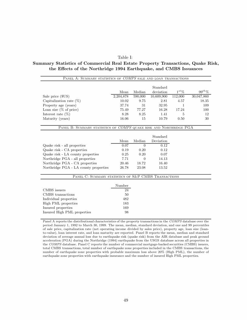
Table I:

Summary Statistics of Commercial Real Estate Property Transactions, Quake Risk,

the Effects of the Northridge 1994 Earthquake, and CMBS Issuances

Panel A: Summary statistics of COMPS sale and loan transactions

Standard

Mean Median deviation 1st% 99th%Sale price ($US) 2,204,878 590,000 10,609,900 112,000 30,047,860Capitalization rate (%) 10.02 9.75 2.81 4.57 18.35Property age (years) 37.74 31 32.95 1 109Loan size (% of price) 75.49 77.27 16.28 17.24 100Interest rate (%) 8.28 8.25 1.41 5 12Maturity (years) 16.06 15 10.79 0.50 30

Panel B: Summary statistics of COMPS quake risk and Northridge PGA

StandardMean Median Deviation

Quake risk - all properties 0.07 0 0.12Quake risk - CA properties 0.19 0.20 0.12Quake risk - LA county properties 0.25 0.20 0.07Northridge PGA - all properties 7.71 0 14.13Northridge PGA - CA properties 20.46 18.72 16.40Northridge PGA - LA county properties 26.78 23.08 13.52

Panel C: Summary statistics of S&P CMBS Transactions

NumberCMBS issuers 24CMBS transactions 50Individual properties 482High PML properties 183Insured properties 169Insured High PML properties 98

Panel A reports the distributional characteristics of the property transactions in the COMPS database over theperiod January 1, 1992 to March 30, 1999. The mean, median, standard deviation, and one and 99 percentilesof sale price, capitalization rate (net operating income divided by sales price), property age, loan size (loan-to-value), loan interest rate, and loan maturity are reported. Panel B reports the mean, median and standarddeviation of average annual loss due to earthquake risk (quake risk) from the AIR database and peak groundacceleration (PGA) during the Northridge (1994) earthquake from the USGS database across all properties inthe COMPS database. Panel C reports the number of commercial mortgage-backed securities (CMBS) issuers,total CMBS transactions, total number of earthquake zone properties included in the CMBS transactions, thenumber of earthquake zone properties with probable maximum loss above 20% (High PML), the number ofearthquake zone properties with earthquake insurance and the number of insured High PML properties.

49

Table II:

Earthquake Risk and Insurance for Securitized Loans

Dependent variable Quake insurance Quake insurance Quake insuranceprovided? provided? provided?

N 482 482 482

High quake risk 1.51 1.41 1.00(7.41) (2.55) (3.04)[35.9%] [33.8%] [24.4%]

Fixed effects?Year Yes Yes YesCMBS issuer No Yes NoCMBS transaction No No Yes

Estimation method Logit Logit Logit

Pseudo R2 0.09 0.09 0.02

Results from the regressions of an indicator for whether earthquake insurance was pro-vided for the property securing the loan on an indicator for properties with probablemaximum loss above 20% (High PML), year dummies and transaction attributes. Thedata is drawn from the S&P CMBS transactions database. The regressions are estimatedvia binary fixed effects (conditional) logistic regression (Logit), as described, with robustt-statistics reported in parentheses. The increase in probability of earthquake insurancebeing provided for High quake risk properties (relative to the mean probability) in givenin square brackets. The reported R2 is McFadden’s pseudo R2.

50

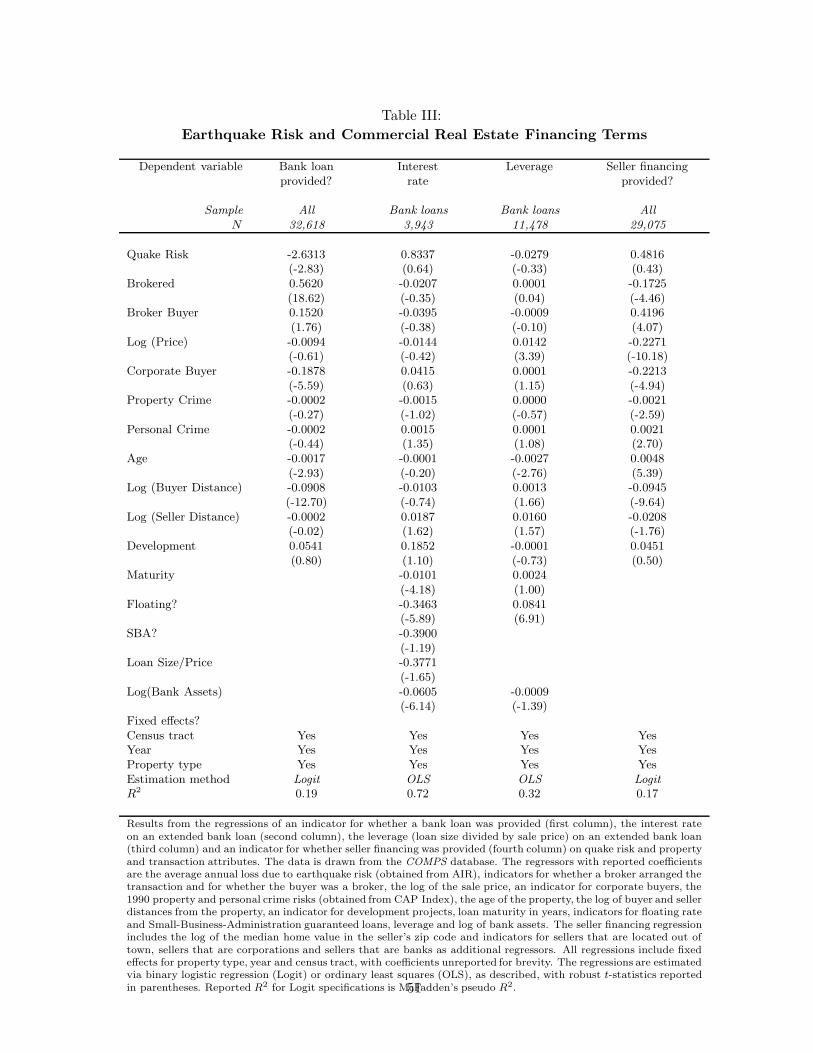
Table III:

Earthquake Risk and Commercial Real Estate Financing Terms

Dependent variable Bank loan Interest Leverage Seller financingprovided? rate provided?

Sample All Bank loans Bank loans All

N 32,618 3,943 11,478 29,075

Quake Risk -2.6313 0.8337 -0.0279 0.4816(-2.83) (0.64) (-0.33) (0.43)

Brokered 0.5620 -0.0207 0.0001 -0.1725(18.62) (-0.35) (0.04) (-4.46)

Broker Buyer 0.1520 -0.0395 -0.0009 0.4196(1.76) (-0.38) (-0.10) (4.07)

Log (Price) -0.0094 -0.0144 0.0142 -0.2271(-0.61) (-0.42) (3.39) (-10.18)

Corporate Buyer -0.1878 0.0415 0.0001 -0.2213(-5.59) (0.63) (1.15) (-4.94)

Property Crime -0.0002 -0.0015 0.0000 -0.0021(-0.27) (-1.02) (-0.57) (-2.59)

Personal Crime -0.0002 0.0015 0.0001 0.0021(-0.44) (1.35) (1.08) (2.70)

Age -0.0017 -0.0001 -0.0027 0.0048(-2.93) (-0.20) (-2.76) (5.39)

Log (Buyer Distance) -0.0908 -0.0103 0.0013 -0.0945(-12.70) (-0.74) (1.66) (-9.64)

Log (Seller Distance) -0.0002 0.0187 0.0160 -0.0208(-0.02) (1.62) (1.57) (-1.76)

Development 0.0541 0.1852 -0.0001 0.0451(0.80) (1.10) (-0.73) (0.50)

Maturity -0.0101 0.0024(-4.18) (1.00)

Floating? -0.3463 0.0841(-5.89) (6.91)

SBA? -0.3900(-1.19)

Loan Size/Price -0.3771(-1.65)

Log(Bank Assets) -0.0605 -0.0009(-6.14) (-1.39)

Fixed effects?Census tract Yes Yes Yes YesYear Yes Yes Yes YesProperty type Yes Yes Yes YesEstimation method Logit OLS OLS Logit

R2 0.19 0.72 0.32 0.17

Results from the regressions of an indicator for whether a bank loan was provided (first column), the interest rateon an extended bank loan (second column), the leverage (loan size divided by sale price) on an extended bank loan(third column) and an indicator for whether seller financing was provided (fourth column) on quake risk and propertyand transaction attributes. The data is drawn from the COMPS database. The regressors with reported coefficientsare the average annual loss due to earthquake risk (obtained from AIR), indicators for whether a broker arranged thetransaction and for whether the buyer was a broker, the log of the sale price, an indicator for corporate buyers, the1990 property and personal crime risks (obtained from CAP Index), the age of the property, the log of buyer and sellerdistances from the property, an indicator for development projects, loan maturity in years, indicators for floating rateand Small-Business-Administration guaranteed loans, leverage and log of bank assets. The seller financing regressionincludes the log of the median home value in the seller’s zip code and indicators for sellers that are located out oftown, sellers that are corporations and sellers that are banks as additional regressors. All regressions include fixedeffects for property type, year and census tract, with coefficients unreported for brevity. The regressions are estimatedvia binary logistic regression (Logit) or ordinary least squares (OLS), as described, with robust t-statistics reportedin parentheses. Reported R2 for Logit specifications is McFadden’s pseudo R2.51

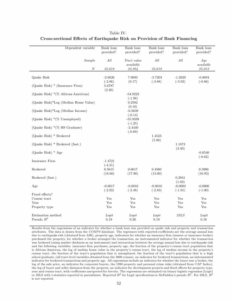
Table IV:

Cross-sectional Effects of Earthquake Risk on Provision of Bank Financing

Dependent variable Bank loan Bank loan Bank loan Bank loan Bank loanprovided? provided? provided? provided? provided?

Sample All Tract value All All Age

available available

N 32,618 22,924 32,618 25,012

Quake Risk -2.6626 7.9693 -3.7203 -1.2629 -0.8694(-2.86) (0.17) (-3.88) (-3.92) (-0.86)

(Quake Risk) * (Insurance Firm) 5.6787(2.20)

(Quake Risk) *(% African-American) -54.8223(-1.98)

(Quake Risk)*Log (Median Home Value) 0.2582(0.10)

(Quake Risk)*Log (Median Income) -0.5638(-0.14)

(Quake Risk) *(% Unemployed) -55.9338(-1.25)

(Quake Risk) *(% HS Graduate) -2.4440(-0.69)

(Quake Risk) * Brokered 1.4523(5.86)

(Quake Risk) * Brokered (Inst.) 1.1873(3.40)

(Quake Risk) * Age -0.0540(-8.62)

Insurance Firm -1.4721(-4.21)

Brokered 0.5615 0.6617 0.4560 0.5900(18.60) (17.90) (13.00) (16.92)

Brokered (Inst.) 0.2941(1.03)

Age -0.0017 -0.0016 -0.0016 -0.0003 -0.0006(-2.92) (-2.48) (-2.83) (-1.91) (-1.00)

Fixed effects?Census tract Yes Yes Yes Yes YesYear Yes Yes Yes Yes YesProperty type Yes Yes Yes Yes Yes

Estimation method Logit Logit Logit 2SLS Logit

Pseudo R2 0.19 0.20 0.19 0.16

Results from the regressions of an indicator for whether a bank loan was provided on quake risk and property and transactionattributes. The data is drawn from the COMPS database. The regressors with reported coefficients are the average annual lossdue to earthquake risk (obtained from AIR), property age, indicators for whether an insurance firm (insurer or insurance broker)purchased the property, for whether a broker arranged the transaction, an instrumented indicator for whether the transactionwas brokered (using market thickness as an instrument) and interactions between the average annual loss due to earthquake riskand the following variables: insurance firm purchaser, property age, the fraction of the property’s census tract population thatis African-American, the log of median home value in the property’s census tract, the log of median income in the property’scensus tract, the fraction of the tract’s population that is unemployed, the fraction of the tract’s population that is a highschool graduate, (all tract-level variables obtained from the 2000 census), an indicator for brokered transactions, an instrumentedindicator for brokered transactions and property age. All regressions include an indicator for whether the buyer was a broker, thelog of the sale price, an indicator for corporate buyers, the 1990 property and personal crime risks (obtained from CAP Index),the log of buyer and seller distances from the property, an indicator for development projects and fixed effects for property type,year and census tract, with coefficients unreported for brevity. The regressions are estimated via binary logistic regression (Logit)or 2SLS with t-statistics reported in parentheses. Reported R2 for Logit specifications is McFadden’s pseudo R2. For 2SLS, R2

is not reported.

52

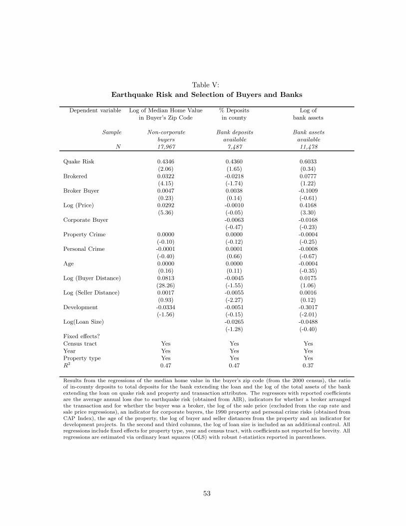
Table V:

Earthquake Risk and Selection of Buyers and Banks

Dependent variable Log of Median Home Value % Deposits Log ofin Buyer’s Zip Code in county bank assets

Sample Non-corporate Bank deposits Bank assets

buyers available available

N 17,967 7,487 11,478

Quake Risk 0.4346 0.4360 0.6033(2.06) (1.65) (0.34)

Brokered 0.0322 -0.0218 0.0777(4.15) (-1.74) (1.22)

Broker Buyer 0.0047 0.0038 -0.1009(0.23) (0.14) (-0.61)

Log (Price) 0.0292 -0.0010 0.4168(5.36) (-0.05) (3.30)

Corporate Buyer -0.0063 -0.0168(-0.47) (-0.23)

Property Crime 0.0000 0.0000 -0.0004(-0.10) (-0.12) (-0.25)

Personal Crime -0.0001 0.0001 -0.0008(-0.40) (0.66) (-0.67)

Age 0.0000 0.0000 -0.0004(0.16) (0.11) (-0.35)

Log (Buyer Distance) 0.0813 -0.0045 0.0175(28.26) (-1.55) (1.06)

Log (Seller Distance) 0.0017 -0.0055 0.0016(0.93) (-2.27) (0.12)

Development -0.0334 -0.0051 -0.3017(-1.56) (-0.15) (-2.01)

Log(Loan Size) -0.0265 -0.0488(-1.28) (-0.40)

Fixed effects?Census tract Yes Yes YesYear Yes Yes YesProperty type Yes Yes YesR2 0.47 0.47 0.37

Results from the regressions of the median home value in the buyer’s zip code (from the 2000 census), the ratioof in-county deposits to total deposits for the bank extending the loan and the log of the total assets of the bankextending the loan on quake risk and property and transaction attributes. The regressors with reported coefficientsare the average annual loss due to earthquake risk (obtained from AIR), indicators for whether a broker arrangedthe transaction and for whether the buyer was a broker, the log of the sale price (excluded from the cap rate andsale price regressions), an indicator for corporate buyers, the 1990 property and personal crime risks (obtained fromCAP Index), the age of the property, the log of buyer and seller distances from the property and an indicator fordevelopment projects. In the second and third columns, the log of loan size is included as an additional control. Allregressions include fixed effects for property type, year and census tract, with coefficients not reported for brevity. Allregressions are estimated via ordinary least squares (OLS) with robust t-statistics reported in parentheses.

53

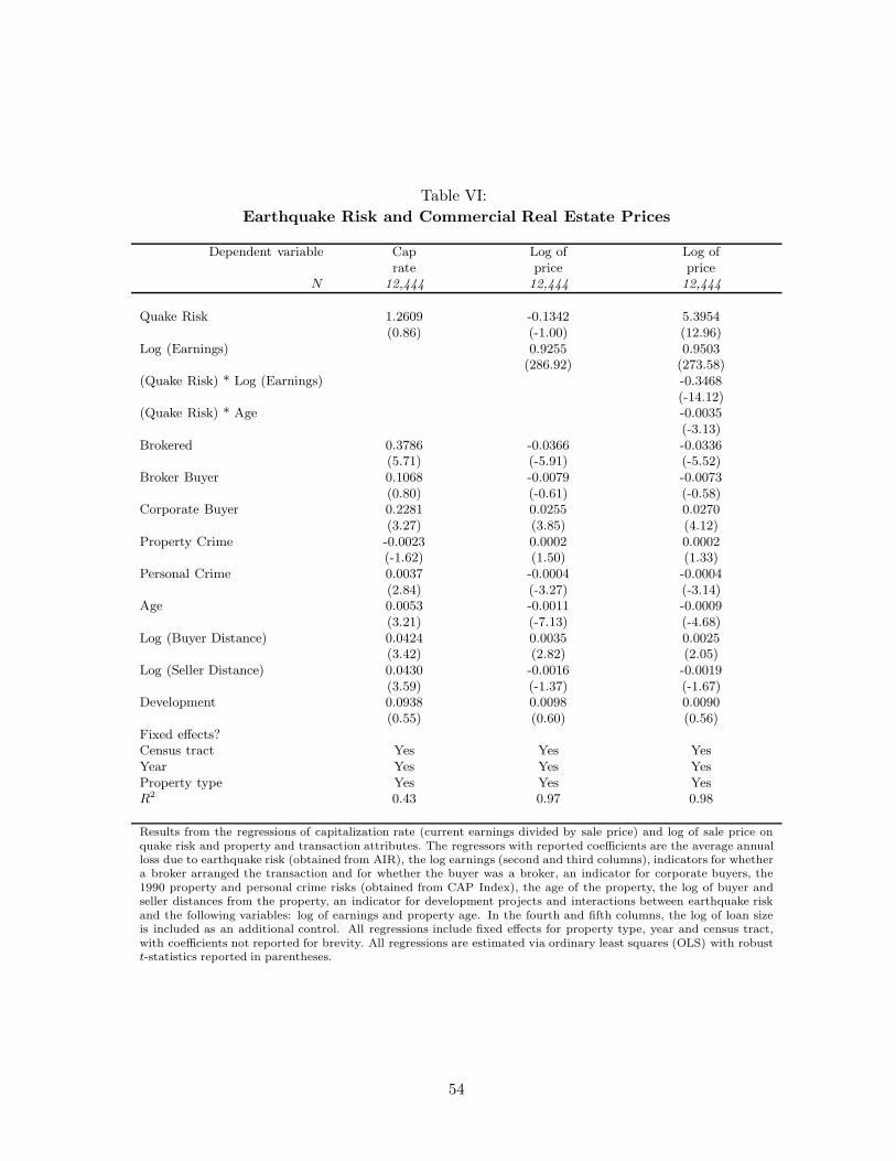
Table VI:

Earthquake Risk and Commercial Real Estate Prices

Dependent variable Cap Log of Log ofrate price price

N 12,444 12,444 12,444

Quake Risk 1.2609 -0.1342 5.3954(0.86) (-1.00) (12.96)

Log (Earnings) 0.9255 0.9503(286.92) (273.58)

(Quake Risk) * Log (Earnings) -0.3468(-14.12)

(Quake Risk) * Age -0.0035(-3.13)

Brokered 0.3786 -0.0366 -0.0336(5.71) (-5.91) (-5.52)

Broker Buyer 0.1068 -0.0079 -0.0073(0.80) (-0.61) (-0.58)

Corporate Buyer 0.2281 0.0255 0.0270(3.27) (3.85) (4.12)

Property Crime -0.0023 0.0002 0.0002(-1.62) (1.50) (1.33)

Personal Crime 0.0037 -0.0004 -0.0004(2.84) (-3.27) (-3.14)

Age 0.0053 -0.0011 -0.0009(3.21) (-7.13) (-4.68)

Log (Buyer Distance) 0.0424 0.0035 0.0025(3.42) (2.82) (2.05)

Log (Seller Distance) 0.0430 -0.0016 -0.0019(3.59) (-1.37) (-1.67)

Development 0.0938 0.0098 0.0090(0.55) (0.60) (0.56)

Fixed effects?Census tract Yes Yes YesYear Yes Yes YesProperty type Yes Yes YesR2 0.43 0.97 0.98

Results from the regressions of capitalization rate (current earnings divided by sale price) and log of sale price onquake risk and property and transaction attributes. The regressors with reported coefficients are the average annualloss due to earthquake risk (obtained from AIR), the log earnings (second and third columns), indicators for whethera broker arranged the transaction and for whether the buyer was a broker, an indicator for corporate buyers, the1990 property and personal crime risks (obtained from CAP Index), the age of the property, the log of buyer andseller distances from the property, an indicator for development projects and interactions between earthquake riskand the following variables: log of earnings and property age. In the fourth and fifth columns, the log of loan sizeis included as an additional control. All regressions include fixed effects for property type, year and census tract,with coefficients not reported for brevity. All regressions are estimated via ordinary least squares (OLS) with robustt-statistics reported in parentheses.

54

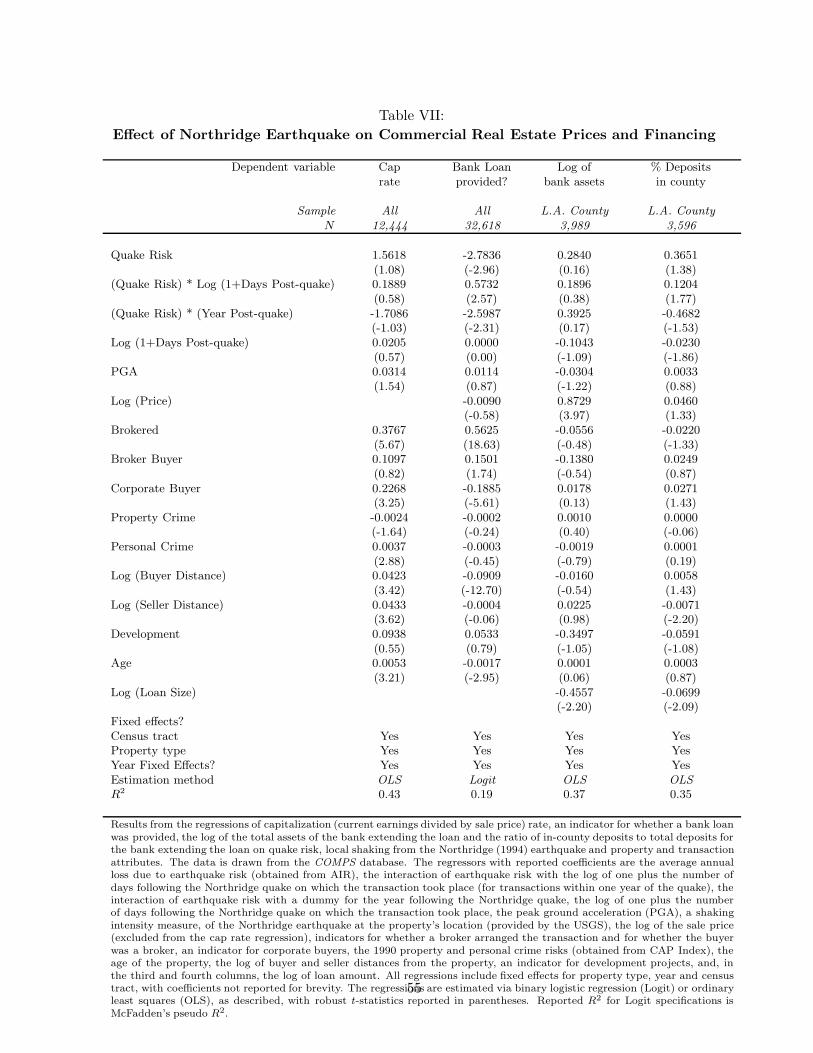
Table VII:

Effect of Northridge Earthquake on Commercial Real Estate Prices and Financing

Dependent variable Cap Bank Loan Log of % Depositsrate provided? bank assets in county

Sample All All L.A. County L.A. County

N 12,444 32,618 3,989 3,596

Quake Risk 1.5618 -2.7836 0.2840 0.3651(1.08) (-2.96) (0.16) (1.38)

(Quake Risk) * Log (1+Days Post-quake) 0.1889 0.5732 0.1896 0.1204(0.58) (2.57) (0.38) (1.77)

(Quake Risk) * (Year Post-quake) -1.7086 -2.5987 0.3925 -0.4682(-1.03) (-2.31) (0.17) (-1.53)

Log (1+Days Post-quake) 0.0205 0.0000 -0.1043 -0.0230(0.57) (0.00) (-1.09) (-1.86)

PGA 0.0314 0.0114 -0.0304 0.0033(1.54) (0.87) (-1.22) (0.88)

Log (Price) -0.0090 0.8729 0.0460(-0.58) (3.97) (1.33)

Brokered 0.3767 0.5625 -0.0556 -0.0220(5.67) (18.63) (-0.48) (-1.33)

Broker Buyer 0.1097 0.1501 -0.1380 0.0249(0.82) (1.74) (-0.54) (0.87)

Corporate Buyer 0.2268 -0.1885 0.0178 0.0271(3.25) (-5.61) (0.13) (1.43)

Property Crime -0.0024 -0.0002 0.0010 0.0000(-1.64) (-0.24) (0.40) (-0.06)

Personal Crime 0.0037 -0.0003 -0.0019 0.0001(2.88) (-0.45) (-0.79) (0.19)

Log (Buyer Distance) 0.0423 -0.0909 -0.0160 0.0058(3.42) (-12.70) (-0.54) (1.43)

Log (Seller Distance) 0.0433 -0.0004 0.0225 -0.0071(3.62) (-0.06) (0.98) (-2.20)

Development 0.0938 0.0533 -0.3497 -0.0591(0.55) (0.79) (-1.05) (-1.08)

Age 0.0053 -0.0017 0.0001 0.0003(3.21) (-2.95) (0.06) (0.87)

Log (Loan Size) -0.4557 -0.0699(-2.20) (-2.09)

Fixed effects?Census tract Yes Yes Yes YesProperty type Yes Yes Yes YesYear Fixed Effects? Yes Yes Yes YesEstimation method OLS Logit OLS OLS

R2 0.43 0.19 0.37 0.35

Results from the regressions of capitalization (current earnings divided by sale price) rate, an indicator for whether a bank loanwas provided, the log of the total assets of the bank extending the loan and the ratio of in-county deposits to total deposits forthe bank extending the loan on quake risk, local shaking from the Northridge (1994) earthquake and property and transactionattributes. The data is drawn from the COMPS database. The regressors with reported coefficients are the average annualloss due to earthquake risk (obtained from AIR), the interaction of earthquake risk with the log of one plus the number ofdays following the Northridge quake on which the transaction took place (for transactions within one year of the quake), theinteraction of earthquake risk with a dummy for the year following the Northridge quake, the log of one plus the numberof days following the Northridge quake on which the transaction took place, the peak ground acceleration (PGA), a shakingintensity measure, of the Northridge earthquake at the property’s location (provided by the USGS), the log of the sale price(excluded from the cap rate regression), indicators for whether a broker arranged the transaction and for whether the buyerwas a broker, an indicator for corporate buyers, the 1990 property and personal crime risks (obtained from CAP Index), theage of the property, the log of buyer and seller distances from the property, an indicator for development projects, and, inthe third and fourth columns, the log of loan amount. All regressions include fixed effects for property type, year and censustract, with coefficients not reported for brevity. The regressions are estimated via binary logistic regression (Logit) or ordinaryleast squares (OLS), as described, with robust t-statistics reported in parentheses. Reported R2 for Logit specifications isMcFadden’s pseudo R2.

55

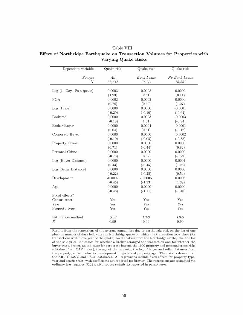
Table VIII:

Effect of Northridge Earthquake on Transaction Volumes for Properties with

Varying Quake Risks

Dependent variable Quake risk Quake risk Quake risk

Sample All Bank Loans No Bank Loans

N 32,618 17,141 15,451

Log (1+Days Post-quake) 0.0003 0.0008 0.0000(1.93) (2.61) (0.11)

PGA 0.0002 0.0002 0.0006(0.78) (0.60) (1.07)

Log (Price) 0.0000 0.0000 -0.0001(-0.20) (-0.10) (-0.64)

Brokered 0.0000 0.0003 -0.0003(-0.13) (1.01) (-0.94)

Broker Buyer 0.0000 0.0004 -0.0001(0.04) (0.51) (-0.12)

Corporate Buyer 0.0000 0.0000 -0.0002(-0.10) (-0.05) (-0.88)

Property Crime 0.0000 0.0000 0.0000(0.71) (-0.44) (0.82)

Personal Crime 0.0000 0.0000 0.0000(-0.73) (0.32) (-0.79)

Log (Buyer Distance) 0.0000 0.0000 0.0001(0.43) (-0.45) (1.26)

Log (Seller Distance) 0.0000 0.0000 0.0000(-0.22) (-0.25) (0.54)

Development -0.0002 -0.0006 0.0006(-0.45) (-1.33) (1.38)

Age 0.0000 0.0000 0.0000(-0.48) (-1.11) (-0.40)

Fixed effects?Census tract Yes Yes YesYear Yes Yes YesProperty type Yes Yes Yes

Estimation method OLS OLS OLS

R2 0.99 0.99 0.99

Results from the regressions of the average annual loss due to earthquake risk on the log of oneplus the number of days following the Northridge quake on which the transaction took place (fortransactions within one year of the quake), local shaking from the Northridge earthquake, the logof the sale price, indicators for whether a broker arranged the transaction and for whether thebuyer was a broker, an indicator for corporate buyers, the 1990 property and personal crime risks(obtained from CAP Index), the age of the property, the log of buyer and seller distances fromthe property, an indicator for development projects and property age. The data is drawn fromthe AIR, COMPS and USGS databases. All regressions include fixed effects for property type,year and census tract, with coefficients not reported for brevity. The regressions are estimated viaordinary least squares (OLS), with robust t-statistics reported in parentheses.

56